Sonderforschungsbereich/Transregio 15 · www.gesy.uni-mannheim.de Universität Mannheim · Freie Universität Berlin · Humboldt-Universität zu Berlin · Ludwig-Maximilians-Universität München Rheinische Friedrich-Wilhelms-Universität Bonn · Zentrum für Europäische Wirtschaftsforschung Mannheim Speaker: Prof. Konrad Stahl, Ph.D. · Department of Economics · University of Mannheim · D-68131 Mannheim, Phone: +49(0621)1812786 · Fax: +49(0621)1812785 July 2003 *Christian Groh, Department of Economics, University of Bonn, Lennestr.37, 53113 Bonn, Germany [email protected]**Benny Moldovanu, Department of Economics, University of Bonn, Lennestr. 37, 53113 Bonn, Germany [email protected]***Aner Sela, Department of Economics, Ben Gurion University, Beer Sheva, Israel, [email protected]****Uwe Sunde, IZA, P.O Box 7240, 53072 Bonn, Germany. [email protected]Financial support from the Deutsche Forschungsgemeinschaft through SFB/TR 15 is gratefully acknowledged. Discussion Paper No. 140 Optimal Seedings in Elimination Tournaments Christian Groh* Benny Moldovanu** Aner Sela*** Uwe Sunde****
Transcript
Sonderforschungsbereich/Transregio 15 · www.gesy.uni-mannheim.de Universität Mannheim · Freie Universität Berlin · Humboldt-Universität zu Berlin · Ludwig-Maximilians-Universität München
Rheinische Friedrich-Wilhelms-Universität Bonn · Zentrum für Europäische Wirtschaftsforschung Mannheim
Speaker: Prof. Konrad Stahl, Ph.D. · Department of Economics · University of Mannheim · D-68131 Mannheim, Phone: +49(0621)1812786 · Fax: +49(0621)1812785
July 2003
*Christian Groh, Department of Economics, University of Bonn, Lennestr.37, 53113 Bonn, Germany [email protected]
**Benny Moldovanu, Department of Economics, University of Bonn, Lennestr. 37, 53113 Bonn, Germany [email protected]
***Aner Sela, Department of Economics, Ben Gurion University, Beer Sheva, Israel, [email protected] ****Uwe Sunde, IZA, P.O Box 7240, 53072 Bonn, Germany. [email protected]
Financial support from the Deutsche Forschungsgemeinschaft through SFB/TR 15 is gratefully acknowledged.
Discussion Paper No. 140
Optimal Seedings in Elimination Tournaments
Christian Groh* Benny Moldovanu**
Aner Sela*** Uwe Sunde****
Optimal Seedings in Elimination Tournaments:
Christian Groh, Benny Moldovanu, Aner Sela and Uwe Sunde∗
31.7.2003
Abstract
We study an elimination tournament with heterogenous contestants whose
ability is common-knowledge. Each pair-wise match is modeled as an all-pay
auction where the winner gets the right to compete at the next round. Equi-
librium efforts are in mixed strategies, yielding rather complex play dynamics:
the endogenous win probabilities in each match depend on the outcome of other
matches through the identity of the expected opponent in the next round. The
designer can seed the competitors according to their ranks. For tournaments
with four players we find optimal seedings with respect to three different crite-
ria: 1) maximization of total effort in the tournament; 2) maximization of the
probability of a final among the two top ranked teams; 3) maximization of the
win probability for the top player. In addition, we find the seedings ensuring
that higher ranked players have a higher probability to win the tournament. Fi-
nally, we compare the theoretical predictions with data from NCAA basketball
Kentucky and Arizona, the highest-ranked teams to reach the Final Four during the
2003 National Collegiate Athletic Association (NCAA) Basketball March Madness,
were on the same bracket and therefore could meet only in the semifinal. Not for the
first time, an emotional debate began: should the Final Four teams be reseeded after
the regional finals, placing the two top teams in separate national semifinals with the
highest ranked team facing the lowest ranked?1
This paper offers a simple game-theoretic model of an elimination tournament
which allows to study the effect of seedings on several performance criteria related to a
tournament’s outcome. For example, our model predicts that the probability of a final
among the two top-ranked teams without reseeding (i.e., as occurring under random
seeding) is in fact equal to the probability of such a final if reseeding is done according
to the method described above2. But, we also predict that such a reseeding will increase
the probability that the top-ranked team actually wins the tournament and show that
there exists a reseeding - different to the one described above - which implies a final
among the two top-ranked teams with probability one. We present these and other
theoretical results and compare some of the obtained predictions with historical data
from the NCAA basketball tournament.
In single elimination (or knockout) tournaments teams or individual players play
pair-wise matches. The winner advances to the next round while the loser is elimi-
nated from the competition. Many sportive events (or their respective final stages,
sometimes called playoffs) are organized in such a way. Examples are the ATP tennis
tournaments, professional playoffs in US-basketball, -football, -baseball and -hockey,
NCAA college basketball, the FIFA (soccer) world-championship playoffs, the UEFA
champions’ league, Olympic disciplines such as fencing, boxing and wrestling, and top-
1For example, a similar event occured in 1996 where the top ranked Kentucky and Massachusetts
also met in a semifinal that was thought to be the ”real” final. For the full story see USA To-
day, March 25, 2003. We assume that all US readers are experts in the mechanics of this tourna-
ment. Ignorants (this group previously included the present authors) can find useful information at
http://www.sportsline.com/collegebasketball/.2That means, the top team meets the lowest ranked team in one semifinal, while the second and
third ranked teams meet in the other.
2
level bridge and chess tournaments. There also numerous elimination tournaments
among students that solve scientific problems, and even tournaments among robots or
algorithms that perform certain tasks. Less rigidly structured variants of elimination
tournaments are also used within firms, for promotions or budgeting decisions, and by
committees who need to choose among several alternatives.
A widely observed procedure in elimination tournaments is to rank competitors
based on some historically observed performance, and then to match them according
to their ranks: the team or player that is historically considered to be best (or ranks
first after some previous stage of the tournament) meets the lowest ranked player, the
second best team meets the second lowest team and so on. In the second round, the
winner of the highest ranked vs. lowest ranked match meets the (expected) lowest
ranked winner from the first round, and so on3. The above design logic is deeply
ingrained in our mind. For example, Webster’s College Dictionary defines the relevant
meaning of the verb ”to seed” as:
”a. to rank (players or teams) by past performance in arranging tour-
nament pairings, so that the most highly ranked competitors will not play
each other until later rounds. b. to arrange (pairings or a tournament) by
means of such a ranking.”
As the above quotation makes clear, the raison d’etre of seeding is to protect top
teams from early elimination: two teams ranked among the top 2N should not meet
until the field has been reduced to 2N or fewer teams. In particular, the two best teams
can meet only in the final, and, with the above seeding method, indeed meet there if
there are no surprises along the way. Presumably, this delivers the most thrilling match
in the final. An outcome where these teams meet in an earlier round greatly reduces
further interest in the tournament and probably does not make financial sense.
From the large literature on contests, however, we know that expected effort and
win probabilities in any two-player contest does not only solely depend on the absolute
strength (or ability) of the respective players, but also on their relative strength (see
3This design is used, for example, in the professional basketball (NBA)- and ice hockey (NHL)-
playoffs.
3
for example Baye et al. (1993)). For example, if the difference in ability between the
best and second-best team is larger than the difference between the second and the
third, a final between the second and third best teams may induce both more effort and
”thrill” (in the sense of more symmetric expected probabilities of winning) than a final
between the two strongest teams. Consequently, there might be (at least theoretically)
rationales for various seedings.
There are many possible seedings in an elimination tournament. The reader may
amuse herself/himself by calculating that, with 2N players, there are (2N )!
2(2N−1)different
seedings. This yields 3 seedings for 4 players, 315 seedings for 8 players, 638.510.000
seedings for 16 players and 6. 126 5×1025 seedings for 32 players.
There is a significant statistical literature on the design of various forms of elim-
ination tournaments (the pioneering paper4 is David (1959) who considered the win
probability of the top player in a four player tournament with a random seeding). This
literature assumes that, for each encounter among players i and j, there is a fixed,
exogenously given probability that i beats j. In particular, this probability does not
depend on the stage of the tournament where the particular match takes place, and
does not depend on the identity of the expected opponent at the next stage5. Most
results in that literature offer formulas for computing overall probabilities with which
various players may win the tournament. For specific numerical examples it has been
noted that the seeding where best meets worst, etc...yields for the top ranked player
a higher probability of winning than a random seeding. Several papers (see for exam-
ple, Hwang (1982), Horen and Reizman (1985) and Schwenk (2000)) consider various
optimality criteria for choosing seedings. Given the sheer number of possible seedings
and match outcomes, there are no general results for tournaments with more than four
players. In particular, the optimal seeding for a given criterion may depends on the
particular matrix of win probabilities (see Horen and Reizman (1985) who consider
general (fixed) win probabilities and analyze tournaments with four and eight players).
In contrast to the above mentioned literature, we consider here a tournament model
4See also Glenn (1960) and Searles (1963) for early contributions.5Additional assumptions are that i′s probability to win against j is larger than vice-versa if i
is higher ranked than j (and thus it is at least 50%), and that the win probability decreases if
the opponent’s rank is increased. Probability matrices satisfying these conditions are called doubly-
monotone.
4
where forward looking agents exert effort in order to win a match and advance to the
next stage. We assume that players have different, common knowledge abilities and
we model each match among two players as an all-pay auction: the prize for the
winner of a particular match is either the tournament’s prize if that match was the
final, or else the right to compete at the next round. As a result, win probabilities
in each match become endogenous - they result from mixed equilibrium strategies,
and are positively correlated to ability. Moreover, the win probabilities depend on the
stage of tournament where the match takes place and on the identity of the future
expected opponents (which are determined in other parallel matches). Thus, in order
to determine the tournament’s outcome, we need to compute an intertwined set of
pair-wise equilibria for each seeding6. In this paper we provide full analytic solutions
for the case of four players (or three different seedings in the semifinals).
Since the players’ ranking is assumed to be common-knowledge, it can be used by
the designer in order to determine the tournament’s seeding structure, and we look
for the optimal seeding from the designer’s point of view. In reality there are many
possible designer’s goals, tailored to the role and importance of the competition, to local
idiosyncracies (such as fan support for a home team), and depending on commercial
contracts with large sponsors (that may be also related to prominent competitors),
or with media companies. We consider here three separate optimality criteria, and,
additionally, a ”fairness” criterion:
1. Find the seeding(s) that maximizes total expected effort in the tournament.
2. Find the seeding(s) that maximizes the probability of a final among the two
highest ranked players.
3. Find the seeding(s) that maximizes the win probability of the highest ranked
player.
4. Find the seeding(s) with the property that higher ranked players have a higher
probability of winning the tournament.
Note that deterministic seedings are inherently ”unfair” since they favor certain
players, while handicapping others. Our first optimality criterion is ”conservative”
6This requires solving for fixed points.
5
in the sense that it treats all matches in the tournament symmetrically, and it does
not a-priori bias the decision in favor of top players. The statistical literature did
not analyze this criterion since there are no strategic decisions (e.g., about effort) in
their models. In contrast, the other two optimality criteria have been discussed in
the statistical literature, and seem to be prevalent in practice. The last criterion (also
discussed in the past) poses a constraint on the unfairness of a seeding by requiring that
the overall win probabilities are naturally ordered according to the players’ ranking.
If this property does not hold for a given seeding, anticipating players have a perverse
incentive to manipulate their ranking (e.g., by exerting less effort in a qualifying stage).
Our main findings are as follows: Let the four players be ranked in decreasing order
of strength: 1,2,3,4. Seedings specify who meets whom in the semifinals. It turns out
that the seeding most observed in practice7, A:1-4,2-3, maximizes the win probability
of the strongest player, and is the unique one with the property that strictly stronger
players have a strictly higher probability of winning (criteria 3 and 4). On the other
hand, seeding B:1-3,2-4 maximizes both total effort across the tournament and the
probability of a final among the two top players (criteria 1 and 2). Seeding C:1-2,3-4,
under which the two top players meet already in the semifinal, does not satisfy any of
the optimality or fairness criteria, and the same holds for a random seeding8.
An important feature of our findings is that the above results do not depend on
cardinal differences between players’ strength (which are hard to measure), but only on
the ordinal ranking specifying who is stronger than whom. This allows us to compare
the theoretical predictions to real-life tournaments where, in most cases, the remaining
players in the semifinals need not be the a-priori highest ranked four players. To un-
derstand the nature of such an exercise, consider the four regional conferences of the
NCAA basketball tournament. In each conference 16 ranked teams play in an elimina-
tion tournament whose winner goes on to play in the national semifinals. Needless to
say, the conference semifinals are not necessarily played by the four originally highest
ranked teams. For example, the 2002 Midwest semifinals where Kansas (1)-Illinois (4)
7This is also the seeding method proposed for the Final Four.8In a recent paper Schwenk (2000) argues for cohort randomized seeding based on three fairness
criteria. In cohort randomized seeding players are first divided in several cohorts according to strength
(say top, middle, bottom) and players in the same cohort are treated symmetrically in the random-
ization.
6
and Oregon (2)-Texas (6). Since the top ranked team (Kansas) played against the third
highest ranked team among the remaining ones (Illinois), this semifinal corresponds to
our seeding B:1-3,2-4. The West semifinals were Oklahoma (2)-Arizona (3) and UCLA
(8)-Missouri (12). Since the two top remaining teams (Oklahoma and Arizona) meet
already in the semifinal, this corresponds to our seeding C:1-2,3-4 . The 2001 South
semifinals were Tennessee (4)-N.Carolina (8) and Miami (6)-Tulsa (7). Since the high-
est ranked remaining team (Tennessee) plays against the lowest ranked remaining one
(N.Carolina), this corresponds to seeding A. In this way, available data can generate
observations for all three possible seedings, even if the initial method of seeding at the
beginning of the tournament is fixed. We find that the data from college basketball
tournaments are broadly in line with our predictions from the game theoretic model
about optimal seeding.
We conclude our Introduction by mentioning several related papers from the eco-
nomics literature. In a classical piece, Rosen (1986) looks for the optimal prize struc-
ture in an elimination tournament with homogeneous players where the probability of
winning a match is a stochastic function of players’ efforts. In the symmetric equilib-
rium, the winner of every match is completely determined by the exogenous stochastic
terms9. In Section IV he also considers an example with four players that can be either
”strong” or ”weak”. Rosen finds (numerically) that a random seeding yields higher
total effort than the seeding where strong players meet weak players in the semifinals.
He did not consider the seeding strong/strong and weak/weak in the semifinals, but, in
his numerical example, it turns out, for example, that this seeding (which corresponds
then to our seeding C:1-2,3-4) yields the highest total effort.
As a by-product of our analysis, we show that total expected effort in the elimi-
nation tournament where the two strongest players meet in the final with probability
one (seeding B:1-3,2-4) equals total effort in the all-pay auction where all players com-
pete simultaneously. This should be contrasted with the main finding of Gradstein
and Konrad (1999) who study a rent-seeking setting a la Tullock with homogenous
players. They found that simultaneous contests are strictly superior if the contest’s
rules are discriminatory enough (as in an all-pay auction). In a setting with heteroge-
9His main result is that rewards in later stages must be higher than reward in earlier stages in
order to sustain a non-decreasing effort along the tournament.
7
nous valuations, our analysis indicates that, for the Gradstein-Konrad result to hold,
it is necessary that the multistage contest induces a positive probability that the two
strongest players do not reach the final (e.g., our seedings A:1-4,2-3 and C:1-2,3-4)
with probability one.
Baye et al. (1993) look for the optimal set of contestants in an all-pay auction,
and they find that it is sometimes advantageous to exclude the strongest player. These
authors do not consider explicit mechanisms by which finalists are selected. Our anal-
ysis suggests that, given the constraints imposed by the structure of an elimination
tournament, it never pays off to exclude the strongest player from the final10.
While we ask which types of players should be in the final, Amegashie (1999)
determines the optimal number of finalists in a two-stage contest a la Tullock with
homogenous players11.
The paper is organized as follows. We present the tournament model in section
2. In section 3 we present the optimality results, and briefly illustrate the employed
techniques. In section 4 we compare the theoretical results with historical data from
the NCAA tournament. In section 5 we gather several concluding remarks. All proofs
and additional remarks concerning the empirical part are in an Appendix.
2 The Model
There are four players (or teams) i = 1, ..., 4 competing for a prize. The prize is
allocated to the winner of a contest which is organized as an elimination tournament.
First, two pairs of players simultaneously compete in two semifinals. The two winners
(one in each semifinal) compete in the final, and the winner in the final obtains the
prize. The losers of the semifinals do not compete further. We model each match among
two players as an all-pay auction: both players exert effort, and the one exerting the
higher effort wins.
10Clark and Riis (1998) show that it does not pay off to exclude the strongest player from a
simultaneous moves contest if there are several prizes.11Increasing the number of finalists has several effects: efforts in the final and also efforts at the
previous stage are lower since the probability of winning the final decreases. But, there is also a
positive effect on effort since the probability of getting to the final increases.
8
Player i values the prize at vi, where v1 ≥ v2 ≥ v3 ≥ v4 > 0. Valuations are
common-knowledge. The heterogeneity in valuations should be interpreted as arising
from heterogeneity in abilities: if effort is less costly for more able contestants, the
players with higher valuations can be thought of as being more able.
We assume that each finalist obtains a payment k > 0, independent from his per-
formance in the final12, and we consider the limit behavior as k → 0. This technicality
is required in order to ensure that all players have positive present values when com-
peting in the semifinals - this is a necessary condition for the existence of equilibria in
the semifinals.
In a final between players i and j, the exerted efforts are ei , ej. Net of k, the
payoff for player i is given by
uFi (ei, ej) =
−ei if ei < ej
vi2 − ei if ei = ej
vi − ei if ei > ej
(1)
and analogously for player j. Player i′s payoff in a semifinal between players i and j is
given by
ui(eSi , eS
j ) =
−eS
i if eSi < eS
j
EuFi + k2 − eS
i if eSi = eS
j
EuFi + k − eS
i if eSi > eS
j .
(2)
and analogously for player j. Note that each player’s payoff in a semifinal depends on
the expected utility associated with a participation in the final. In turn, this expected
utility depends on the expected opponent in the final. It is precisely this feature that
can be ”manipulated” by designing the seeding of the semifinals. The contest designer
chooses the structure s of the semifinals out of the set of feasible seedings {A, B, C} ,
where:
• A:1-4,2-3
• B:1-3,2-4
12There are many examples where such a feature is indeed present.
9
• C:1-2,3-4.
The following well-known Lemma characterizes behavior in an all-pay auction
among two heterogenous players.
Lemma 1. Consider two players i and j with 0 < vj ≤ vi that compete in an all-pay
auction for a unique prize. In the unique Nash equilibrium both players randomize on
the interval [0, vj]. Player i’s effort is uniformly distributed, while player j ’s effort is
distributed according to the cumulative distribution function13 Gj(e) = (vi− vj + e)/vi.
Given these mixed strategies, player i′s winning probability against j is given by qij =
1 − vj
2vi. Player i’s expected effort is
vj
2, and player j’s expected effort is
v2j
2vi. Total
expected effort is therefore
vj
2(1 +
vj
vi
). (3)
The respective expected payoffs are
ui = vi − vj (4)
and
uj = 0. (5)
Proof. See Hillman and Riley (1989) and Baye et al. (1993).
13Note that this distribution has an atom of size (vi − vj)/vi at e = 0.
10
3 Semifinals Design
We provide here optimal seedings for the last crucial stage requiring design - the semi-
finals. Recall that the proponents of a change in the March Madness rules suggest to
design the national semifinals after the results of the previous stages become known-
thus our model precisely provides tools for assessing a change in the rules.
We first verbally sketch the main intuition behind the results. We next offer an
illustration for the simple special case where there are two equally strong and two
equally weak players (this can be compared to Rosen’s example mentioned in the
Introduction). Finally, we present the general optimality results for the various criteria.
3.1 Intuition
Let us first look at design A:1-4,2-3. As k goes to zero, player 1 reaches the final
with almost certainty. This happens because player 4 expects a limit payoff of zero
no matter which player (either 2 or 3) she meets in a final. A-priori, players 2 and 3
are not in a symmetric position: while both would obtain a limit payoff of zero in a
final against player 1, their expected payoffs are positive but different in a final against
player 4 (with 2 having the higher valuation). But, since the event of meeting 4 in
a final has a zero limit probability, the position of 2 and 3 becomes symmetric: since
both know that they are going to meet the stronger player 1 in the final, their limit
expected valuation for the final is zero. Hence, both reach the final with probability
one-half and meet there player 1.
In design B:1-3,2-4, player 4 has a limit expected utility of zero in any final (where
he meets either 1 or 3 - both stronger players), whereas player 2 has a positive expected
value stemming from the event where he might meet player 3 in the final. In the limit,
player 2 reaches the final with probability one. But then, player 3 does not expect a
positive payoff in the final. Hence, player 1 reaches the final with probability one, and
meets there player 2.14
14Of course, as k gets small, neither 2 nor 4 have a positive valuation for the final where they meet
player 1 for sure; but player 2’s valuation converges to zero at a slower rate, confirming the above
logic.
11
Since the expected final in design B:1-3,2-4 (among players 1 and 2 ) is tighter
than the expected final in design A:1-4,2-3 (where 1 meets either 2 or 3 , each with
probability one-half), design B:1-3,2-4 dominates design A:1-4,2-3 with respect to total
effort. However, the comparison between seedings B:1-3,2-4 and C:1-2,3-4 with respect
to total effort is more subtle.
In design C:1-2,3-4 all four possible finals have a positive probability since both
stronger players expect a positive payoff in a final , and both weak players expect a
zero payoff. An important observation is that a semifinal among players 1 and 2 yields
less total effort than a final among these players because both players anticipate that,
in order to ultimately win the tournament, they need to exert an additional effort in
the final. The decrease in effort caused by the fact that 1 and 2 meet already in the
semifinal cannot be compensated by the additional effort in a final among one of the
stronger players and one of the weaker players, and seeding B:1-3,2-4 also dominates
seeding C:1-2,3-4 with respect to total effort.
Recall that in seeding B:1-3,2-4 there is a final among players 1 and 2 with limit
probability one. Hence, player 1’s overall win probability equals the probability with
which he wins a final against player 2. In seeding A:1-4,2-3 player 1 also reaches the
final with limit probability one, but meets there either player 2 or player 3 (with equal
limit probabilities). Since player 1 is more likely to win a final against player 3 than a
final against player 2, we easily obtain that seeding A:1-4,2-3 clearly dominates seeding
B:1-3,2-4 with respect to the top player’s win probability.
The comparison between seedings C:1-2,3-4 and A:1-4,2-3 with respect to the top
player’s win probability is more subtle: player 1 is more likely to win the final in seeding
C:1-2,3-4 (where he meets either player 3 or player 4) than in seeding A:1-4,2-3 (where
he meets either 2 or 3) . But, in seeding A:1-4,2-3 player 1 makes it to the final for
sure, while in seeding C :1-2,3-4 only with some probability less than one (since he
first has to win the semifinal against player 2). It turns out that this last handicap is
significant, and it is always the case that seeding A:1-4,2-3 yields a higher overall win
probability for player 1.
12
3.1.1 The Two-Type Case
We briefly consider here the case where v1 = v2 = vH > vL = v3 = v4. Obviously,
seedings A:1-4,2-3 and B:1-3,2-4 are here equivalent.
Seedings A:1-4,2-3 and B:1-3,2-4. Let qSij(k) denote the probability that i beats
j in a semifinal among i and j. Based on these probabilities we can compute expected
values for the final, conditional on winning a semifinal. By Lemma 1, the winning
probabilities qSij are themselves determined by these conditional expected values. Thus,
the equilibrium is found by solving for a fixed-point.
Conditional on winning the semifinal, player 1 faces player 2 in the final with
probability qS23(k). This results in a payoff of zero for both finalists since they are of
equal strength. Player 1 meets player 3 in the final with probability 1− qS23(k). Since
3 has valuation vL < vH , player 1 expects a payoff of vH − vL in that case. In any case,
there is the additional payoff k for making it to the final. Thus, player 1’s expected
value from winning the semifinal is given by
qS23(k) · 0 + (1− qS
23(k))(vH − vL) + k = (1− qS23(k))(vH − vL) + k. (6)
Analogously, the expected value for player 2 is given by
(1− qS14(k))(vH − vL) + k, (7)
In the final Player 4 faces player 2 with probability qS23(k) and player 3 with probability
1− qS23(k). Player 4’s expected payoff is k in both cases, and analogously for player 3.
Given the above computed values, Lemma 1 tells us that the winning probabilities
qS14(k) and qS
23(k) are determined by the following equations:
qS14(k) = 1− k
2[(1− qS23(k))(vH − vL) + k]
(8)
and
qS23(k) = 1− k
2[(1− qS14(k))(vH − vL) + k]
. (9)
Solving the above system (under the restriction q ∈ [0, 1]) yields the symmetric solution
qS14(k) = qS
23(k) = 1 +k
2(vH − vL)− 1
2(vH − vL)
√(2(vH − vL) + k)k (10)
13
By Lemma 1, in each of the two semifinals the expected effort is given by
1
2k +
1
2
k2
(1− qS(k))(vH − vL) + k(11)
where q(k) ∈ {qS14(k), qS
23(k)}. Note that
limk→0
qS14(k) = lim
k→0qS23(k) = 1 (12)
Intuitively, the weak players have only a small chance to win the final, and hence exert
almost no effort. This implies that the strong players do not have to exert a lot of
effort in the semifinals either. Moreover, each of the strong players knows that he is
going to meet the other strong player in the final (and thus that the payoff from the
final will be low). This reduces the strong players’ valuation for winning the semifinals.
Players 1 and 2 meet in the final with probability 1 (as k tends to zero). Since
both 1 and 2 have the same valuation vH , total expected effort in the final is vH .
Seeding C:1-2,3-4. The final will be between a player with valuation vH and a
player with valuation vL. Hence, by Lemma 1, expected effort in the final is vL
2
(1 + vL
vH
).
Consider first the semifinal between the strong players 1 and 2. Since the winner of
this semifinal will meet a weak player in the final, both 1 and 2 expect a payoff vH−vL+k
in the final. By Lemma 1 , total expected effort in this semifinal is vH − vL + k (note
that, for small k, this is less than total effort in a final among two strong players, which
yields a total effort of vH).
Consider now the semifinal between the weak players. Both have an expected
payoff of k in the final since this is the payoff in a final against a strong competitor
with valuation vH . Hence, total expected effort in this semifinal is also k.
Total limit effort in seeding C:1-2,3-4 is thus given by:
TEC = limk→0
[1
2vL
(1 +
vL
vH
)+ vH − vL + 2k] = vH − 1
2vL
(1− vL
vH
)(13)
We can conclude that
TEA = TEB = vH > vH − 1
2vL
(1− vL
vH
)= TEC . (14)
14
3.2 Total Effort
We now return to the general four-player case, and we assume first that the designer
chooses the seeding s in order to maximize total expected tournament effort TEs . Let
R be the set of all players, and let F (s) be the set of players reaching the final for a
given seeding s. The designer solves
maxs∈{A,B,C}
{∑i∈R
eSi +
∑i∈F (s)
eFi } (15)
Proposition 1. For any valuations, the limit total tournament effort (as k goes to
zero) is maximized in seeding B:1-3,2-4, where it equals 12(v2 +
v22
v1) . This also equals
the total effort in a one-shot simultaneous contest among all players15.
Proof: See Appendix.
3.3 Probability of a Final among the Two Top Players
We now assume that the designer chooses the seeding s in order to maximize the
probability of a final among the two top players. As already indicated in the previous
section, seeding B:1-3,2-4 is again optimal.
Proposition 2. For any valuations, a final among players 1 and 2 occurs with limit
probability one in seeding B:1-3,2-4, and with limit probability of one-half in seeding
A :1-4, 2-3.16
Proof: See Lemmas 2, 3, 4 in the Appendix.
Interestingly, our model predicts that the probability of a final among the two top
players under random seeding (which roughly corresponds to the method now employed
by the NCAA for the Final Four) is 13(1 + 1
2+ 0) = 1
2, which equals the probability of
such a final under seeding A:1-4,2-3. Thus, reseeding according to A:1-4,2-3 is not likely
15This ”revenue-equivalence” result is interesting from a theoretical point of view; at least in sports
it is not feasible to organize a simultaneous contest among all participants.16The probability for seeding C :1-2,3-4 is obviously zero.
15
to increase the probability of a final among the two top players, but, as we show in the
next section, it will increase the probability that the top team wins the tournament.
Let us briefly discuss the relevance of the above finding for elimination tournaments
among 2N players where N > 2 is the number of rounds needed to produce a winner.
Order the agents by their valuations v1 ≥ v2... ≥ v2N Let Mij denote a match
among players i and j, and let Mw(ij)(hl) denote a match among the winners in the
matches Mij and Mhl.
Definition 1. We say that seeding s eliminates player i in round l < N if, as k tends
to zero, the probability that i reaches stages l + 1 (given that she reached stage l) tends
to zero. Obviously, at most 2N−l players can be eliminated at stage l.
For example, recall our results for round l = 1 of a tournament with 4 players (see
Lemmas 2, 3 and 4 in the Appendix): Seeding C:1-2,3-4 does not eliminate any player,
and all four possible finals have positive probability. Seeding A :1-4,2-3 eliminates only
player 4 and the finals 1-2 and 1-3 have both positive probability. Finally, the optimal
seeding B :1-3,2-4 eliminates both players 3 and 4, and only the final 1-2 has positive
probability (one).
It turns out that it is always possible to seed the players such that the two strongest
players participate in the final with probability one (as k tends to zero). Consider for
example a tournament among 8 players with the following structure of matches: Round
1: M18, M27, M36, M45;Round 2: Mw(18)(36), M
w(27)(45); Round 3: final among winners in
semifinals. It is easy to see that players 6, 7 and 8 are eliminated at stage 1. This
seeding does not eliminate players 4 and 5 at stage 1 since they are in symmetric
positions given their possible future opponents. Thus we obtain either the semifinals
1-3,2-4 or 1-3,2-5. By the logic of seeding B:1-3,2-4, the two respective weaker players
get eliminated in stage 2, and we again obtain the desired final among the two best
players.
It is important to note that, whereas in the four-player case seeding B:1-3,2-4 was
the unique one with the property that it ensures a final among the two best players,
there is more design freedom if there 2N > 4 players.
Finally, we conjecture that any seeding where the two top players meet in the final
16
for sure is also maximizing total expected effort.
3.4 The Top Player’s Win Probability
Seeding B:1-3,2-4 was found to be optimal for the previous two criteria. But recall that
seeding A:1-4,2-3 is the one most often observed in real tournaments. It is reassuring
to find that seeding A:1-4,2-3 is optimal with respect to the important criterion of
maximizing the top player’s win probability.
Proposition 3. For any valuations, player 1’s limit win probability (as k goes to zero)
is maximized in seeding A:1-4,2-3.
Proof: See Appendix.
3.5 Fairness
We now study the win probabilities of all players, and check which seedings have the
property that the probabilities to win the tournament are naturally ordered according
to the players’ ranking.
Proposition 4. Let pi(s) denote the probability that player i wins the tournament for
a given seeding s ∈ {A, B, C}. We have:
1. p1(A) > p2(A) > p3(A) > p4(A);
2. p1(B) > p2(B) > p3(B) = p4(B) = 0.
3. In seeding C :1-2,3-4 it may happen that vi > vj but pi(s) < pj(s).
Proof: See Appendix.
4 Some Empirical Observations
Do these theoretical results bear any empirical relevance? To investigate the empirical
content of the theory presented above, we confront the theoretical propositions with
17
the data from 100 regional NCAA college basketball tournament already mentioned
in the introduction. The data contain results for semi-finals and finals of the four
regional tournaments (East, West, Midwest, South) over the period 1979 to 2003. All
16 participating teams in the respective regional elimination tournaments are initially
ranked according to their previous performance during the selection process. This
allows to identify seedings A:1-4, 2-3, B:1-3,2-4 or C:1-2,3-4 at the stage of semifinals
using the rankings as proxy for the teams’ valuations.17 The availability of a ranking
of the teams in each region at the beginning of the respective tournament allows to
construct a relative ordering of the four teams left in the semi-finals, and to reveal
the seeding of the tournament at the level of semi-finals. Because already two rounds
have been played prior to the semi-final, and only those teams who won elimination
tournaments on the previous levels are left, the seedings are presumably random and
unaffected by the initial seeding of the tournament.18 As shown in Table 1, we observe
all seedings, although A:1-4,2-3 (41 observations) and B:1-3,2-4 (44 observations) are
almost three times more common than C:1-2,3-4 (15 observations).
17Data and relevant links can be found on the internet under
http://old.sportsline.com/u/madness/2002/history/index.html. During the selection process, the
basketball selection committee elects the 64 “best” college teams of the respective season and
allocates them to the regional conferences. This selection is based on several measures reflecting the
teams’ recent performance, including a “rating percentage index”. In principle, the teams are then
split into groups of four according to their ranking. The four highest ranked teams are allocated to the
four regions, always only one team to one region, followed by the split of the next group of four teams,
etc., until all teams are allocated to regions. The aim of this procedure is to balance the brackets in all
regions. The regional brackets are initially seedings of type A of the respective 16 teams. Teams’ re-
gional allocation may change from one year to another. Details about rules and working of the college
basketball championship are contained in the respective Division I Men’s Basketball Championship
Handbook, available on the internet under http://www.ncaa.org/library/handbooks/basketball/2003.18This is only true if ordinal seedings are concerned, as is the case here. Particular combinations
regarding the cardinal ranking of teams, e.g. semifinals among the two strongest regional teams, are
not possible as consequence of the seeding A of regional brackets. We make the identifying assumption
that during the first two rounds of the tournament there is sufficient noise in the match outcomes
to generate a random selection of teams, and thus (ordinal) seedings. We also analyzed a modified
sample to test the robustness of the results and to rule out any potential biases due to selection effects
stemming from initial seedings. In particular, we excluded teams that could only achieve a certain
relative rank in the semi-final in a particular seeding as consequence of the initial seeding, see the
appendix 6.4 for details. The results are qualitatively identical to those obtained from the full sample.
18
The first testable implication of the theory is a consequence of Lemma 1 and states
that, everything else equal, the weaker the underdog compared to the favorite, the
higher the lower the total effort they exert in an all-pay auction, i.e. during a match
(regardless whether semi-final or final). The main problem with testing theoretical
predictions about effort exertion, however, is to find a good and observable proxy for
effort. This is particularly difficult for such a complex team sport as basketball.19
Taking the number of scored points as indicator for effort, one implicitly assumes that
effort mostly reflects offensive effort, but neglects that higher effort might mean better
defense, that is fewer points scored by the rival team. Comparing the number of scored
points across matches teams with different relative rankings, displayed in Table 2, effort
is indeed higher if more equal teams play against each other, or, respectively, better
ranked underdogs play against a particular favorite, as predicted by theory. While the
differences in means are not significant at conventional levels, the null that the number
of points scored is the same regardless of the pairing is rejected in favor of the order
suggested by the theory at the 1 percent level using a Jonckheere-Terpstra-test.20
Testing the result of Proposition 1 that seeding B:1-3,2-4 maximizes total tourna-
ment effort causes similar problems regarding the measuring of effort. Again, when
looking at the total sum of points as proxy of effort as depicted in Table 1, the data
support the theory, but the differences are not significant.21
Proposition 2 before claimed that the probability of a final between the two rela-
tively strongest teams of the semi-finalists is higher in seeding B:1-3,2-4 than in A:1-4,
2-3 (while it is zero by definition in C:1-2,3-4 ). A look at the data provides little sup-
port for this claim: Under seeding B:1-3,2-4, 22 out of 44 observed finals are between
the two highest ranked teams, while under seeding A:1-4,2-3 23 out of 41 finals involve
the two strongest teams. However, closer inspections suggest that this difference is not
significant: A dummy for seed A:1-4,2-3 turns out to be positive but insignificant in
logit estimates of the event of a final between teams 1 and 2, and remains so when a
19In a well known study about the incentive effects of prizes in tournaments, Ehrenberg and Bog-
nanno (1990) looked at golf tournaments. Their proxy for effort was the number of hits required for a
round. In contrast to their application, basketball is more complex, since offensive and defensive are
important, tactics plays a role, partly influenced by the composition of a team and its rival team, etc.20The null of irrelevance of the pairings is also rejected when different groups of pairings are com-
pared to each other.21Experiments with alternative proxies for effort yield similar results.
19
full set of year or regional dummies are included as explanatory variables.22
A further testable result of the theory is that the probability of the strongest team
winning the tournament is maximized by seeding A:1-4,2-3, see Proposition 3. Raw
data mildly support this hypothesis: Under seeding A:1-4,2-3, the best team wins the
tournament in 22 out of 41 cases, under seeding B:1-3,2-4 only in 18 out of 44 cases.
However, in 9 out of 15 cases, the strongest team wins the tournament under seeding
C:1-2,3-4 . To investigate this result in more depth, we adopt a modified version of
the framework suggested by Klaassen and Magnus (2003) to forecast the winner of a
tennis match. To test the influence of seedings on the winning probability of the best
team in the tournament, we estimate a logit model of this event on a modified measure
of ranks based on the expected round of elimination of a team as well as the respective
seed.23 Compared to seeding A:1-4, 2-3, both seeding B:1-3,2-4 and C:1-2,3-4 entail a
significantly smaller probability of the strongest team winning the tournament. While
the respective coefficient for seeding B:1-3,2-4 is significant only on the 10 percent
level, the coefficient for seeding C:1-4,2-3 is significant at the 5 percent level. This
result corroborates the theoretical claim.
As final result, Proposition 4 implies that the probability of winning the tournament
is positively correlated with the ranking of the teams. The raw frequencies of winner
types by seeding displayed in Table 1 illustrate that this prediction is approximately
corroborated by the data. Higher ranked teams are more likely to win a tournament.
The only seeding for which this relationship is not strictly monotonous, is seeding
C:1-2,3-4 , which is in line with the theoretical prediction.
To sum up, data from college basketball tournaments are broadly in line with the
predictions from the game theoretic model about optimal seeding presented above.
22The control group is seed B, the number of observations is 85.23The modified measure of ranks is based on the round in which a team is expected to lose and drop
out of the tournament. The rank of a team i, ri, is given by ri = 2 − log2(ranki). The probability
of winning the final is a function of the own rank of a finalist team as well as of the rank of the
competing finalist team, rj . The estimated specification is a logit model of the probability that the
team ranked 1 prior to the tournament wins the final. The number of observations is 100. In addition
to the difference in modified ranks, d = ri− rj used by Klaassen and Magnus (2003), we use dummies
for seedings B and C as explanatory variables. As in the Klaassen and Magnus paper, the effect of
the rank difference d is positive and significant.
20
However, not all implications are reflected in the data. This has to do with practical
difficulties to come up with a satisfactory empirical proxy for effort. Moreover, other
factors than the respective seeding shape the tournament outcomes, so that it is difficult
to identify any direct causal effects of seedings on teams’ performance or the observed
tournament results. Finally, due to data limitations, it is difficult to perform more
detailed tests, leading to statistically more significant results. Therefore, the empirical
observations reported here are to be taken as corroborating evidence for the relevance
of the problem and the applicability of the theoretical results, rather than a concise
test of the theory.
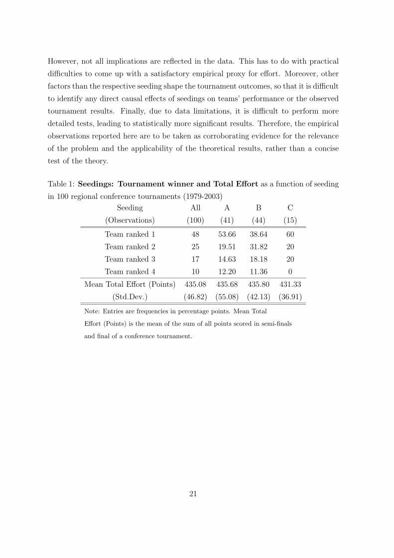
Table 1: Seedings: Tournament winner and Total Effort as a function of seeding
in 100 regional conference tournaments (1979-2003)
Seeding All A B C
(Observations) (100) (41) (44) (15)
Team ranked 1 48 53.66 38.64 60
Team ranked 2 25 19.51 31.82 20
Team ranked 3 17 14.63 18.18 20
Team ranked 4 10 12.20 11.36 0
Mean Total Effort (Points) 435.08 435.68 435.80 431.33
(Std.Dev.) (46.82) (55.08) (42.13) (36.91)
Note: Entries are frequencies in percentage points. Mean Total
Effort (Points) is the mean of the sum of all points scored in semi-finals
and final of a conference tournament.
21
Table 2: Relative Strength of Teams: Composition of Finals and Total Effort
in 100 regional conference tournaments (1979-2003)
Composition of Finals Total Points per Match
Match All Seeding A Seeding B Seeding C Mean Std.Dev.
1 vs 2 45 56.10 50.00 0 149.06 24.23
1 vs 3 15 24.39 0 33.33 148.54 22.81
1 vs 4 15 0 20.45 40.00 144.30 20.63
2 vs 3 10 0 15.91 20.00 142.16 22.39
2 vs 4 3 4.88 0 6.67 141.74 21.95
3 vs 4 12 14.63 13.64 0 141 21.11
Note: Entries for composition of finals are in percentage points.
5 Concluding Remarks
We have analyzed optimal seedings in an elimination tournament where players have to
exert effort in order to advance to the next stage. We established that seedings involving
a delayed encounter among the top players are optimal for a variety of criteria. We
have also exhibited the effects of switching the ranks of the opponents that play against
the top players in the semifinals. In principle, it is possible to generalize the analysis
conducted here to tournaments with more players (and possibly more prizes). But,
the exponentially growing number of seedings, and the complexity of the fixed-point
arguments suggest that analytic solutions are difficult to come by.
Our model and results offer a wealth of testable hypothesis. We have compared its
predictions to the results of the NCAA basketball tournaments. In a companion paper
we look at a data set containing 150 ATP tennis tournaments
6 Appendix
All results are based on the three basic lemmas that determine equilibrium behavior
for each seeding. Let qSij(k) denote the limit probability that i beats j if they meet in
a semifinal, and let qSij = limk→0 qS
ij(k). TESij(k) denotes total equilibrium effort in a
22
semifinal among i and j; TEFs (k) denotes total equilibrium effort in a final resulting
from seeding s; TEs(k) denotes total equilibrium effort in all three matches of seeding
s, and define TEs = limk→0 TEs(k);
Lemma 2. Consider seeding A :1-4,2-3 . In the limit, as k → 0, player 1 reaches the
final with probability one, while players 2 and 3 reach the final with probability one-half
each. In addition the following hold:
limk→0
(TES14(k) + TES
23(k)) = 0 (16)
and
TEA = limk→0
TEA(k) = limk→0
TEFA (k) =
1
4
(v2 +
v22
v1
+ v3 +v2
3
v1
)(17)
Proof: By equations (4) and (5), player 1’s valuation for the semifinal is (1 −qS32(k))(v1− v2 + k) + qS
32(k)(v1− v3 + k) and player 4’s valuation is k. By equation (3),
we know that the total expected effort in this semifinal is given by
TES14(k) =
1
2k +
1
2
k2
(1− qS32(k))(v1 − v2 + k) + qS
32(k)(v1 − v3 + k) + k. (18)
Player’s 4 probability of winning is given by
qS41(k) =
1
2
k
(1− qS32(k))(v1 − v2 + k) + qS
32(k)(v1 − v3 + k) + k(19)
Players 2 and 3 play in the other semifinal. Their valuations for the semifinal are
qS41(k)(vj − v4 +k)+ (1− qS
41(k))k, j = 2, 3 , and expected total efforts in this semifinal
is given by
TES23(k) =
1
2[qS
41(k)(v3 − v4 + k) + (1− qS41(k))k] +
1
2
(qS41(k)(v3 − v4 + k) + (1− qS
41(k))k)2
qS41(k)(v2 − v4 + k) + (1− qS
41(k))k(20)
Player’s 3 probability of winning is given by
qS32(k) =
1
2
qS41(k)(v3 − v4 + k) + (1− qS
41(k))k
qS41(k)(v2 − v4 + k) + (1− qS
41(k))k. (21)
23
In the limit, as k → 0, the unique fixed point is qS41 = 0 and qS
32 = 1/2. We have then
TEFA =
1
4
(v2 +
v22
v1
+ v3 +v2
3
v1
)
Q.E.D.
Lemma 3. Consider seeding B:1-3,2-4. In the limit, as k → 0, the final takes place
among players 1 and 2 with probability one. In addition, the following hold:
limk→0
(TES13(k) + TES
24(k)) = 0 (22)
and
TEB = limk→0
TEB(k) = limk→0
TEFB(k) =
1
2(v2 +
v22
v1
) (23)
Proof: Player 1’s valuation for the semifinal is (1−qS42(k))(v1−v2+k)+qS
42(k)(v1−v4 + k) and player 3’s valuation is (1− qS
42(k))k + qS42(k)(v3 − v4 + k). Total expected
effort in this semifinal is given by
TES13(k) =
1
2((1− qS
42(k))k + qS42(k)(v3 − v4 + k)) +
1
2
((1− qS42(k))k + qS
42(k)(v3 − v4 + k))2
(1− qS42(k))(v1 − v2 + k) + qS
42(k)(v1 − v4 + k)(24)
Player’s 3 probability of winning is given by
qS31(k) =
1
2
(1− qS42(k))k + qS
42(k)(v3 − v4 + k)
(1− qS42(k))(v1 − v2 + k) + qS
42(k)(v1 − v4 + k)(25)
Players 2 and 4 play in the other semifinal. Their valuations for the semifinal are
qS31(k)(v2− v3 + k) + (1− qS
31(k))k for player 2 and k for player 4. Expected total effort
in this semifinal is given by
TES24(k) =
1
2k +
1
2
k2
qS31(k)(v2 − v3 + k) + (1− qS
31(k))k. (26)
Player’s 4 probability of winning the semifinal is given by
q42(k) =1
2
k
q31(k)(v2 − v3 + k) + (1− q31(k))k. (27)
24
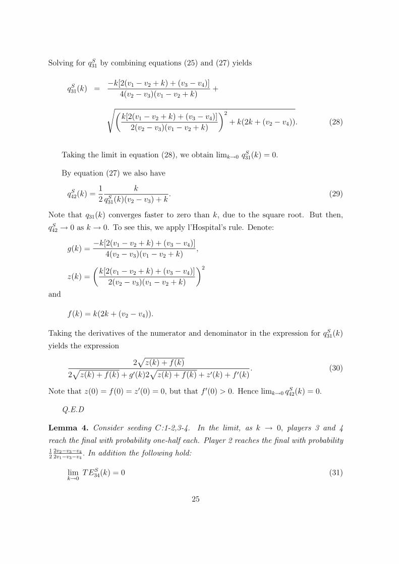
Solving for qS31 by combining equations (25) and (27) yields
qS31(k) =
−k[2(v1 − v2 + k) + (v3 − v4)]
4(v2 − v3)(v1 − v2 + k)+
√(k[2(v1 − v2 + k) + (v3 − v4)]
2(v2 − v3)(v1 − v2 + k)
)2
+ k(2k + (v2 − v4)). (28)
Taking the limit in equation (28), we obtain limk→0 qS31(k) = 0.
By equation (27) we also have
qS42(k) =
1
2
k
qS31(k)(v2 − v3) + k
. (29)
Note that q31(k) converges faster to zero than k, due to the square root. But then,
qS42 → 0 as k → 0. To see this, we apply l’Hospital’s rule. Denote:
g(k) =−k[2(v1 − v2 + k) + (v3 − v4)]
4(v2 − v3)(v1 − v2 + k),
z(k) =
(k[2(v1 − v2 + k) + (v3 − v4)]
2(v2 − v3)(v1 − v2 + k)
)2
and
f(k) = k(2k + (v2 − v4)).
Taking the derivatives of the numerator and denominator in the expression for qS31(k)
yields the expression
2√
z(k) + f(k)
2√
z(k) + f(k) + g′(k)2√
z(k) + f(k) + z′(k) + f ′(k). (30)
Note that z(0) = f(0) = z′(0) = 0, but that f ′(0) > 0. Hence limk→0 qS42(k) = 0.
Q.E.D
Lemma 4. Consider seeding C:1-2,3-4. In the limit, as k → 0, players 3 and 4
reach the final with probability one-half each. Player 2 reaches the final with probability12
2v2−v3−v4
2v1−v3−v4. In addition the following hold:
limk→0
TES34(k) = 0 (31)
25
limk→0
TES12(k) =
1
4[(2v2 − v3 − v4) +
(2v2 − v3 − v4)2
2v1 − v3 − v4
] (32)
TEC = limk→0
TEC(k) =1
2v2 +
1
4
(v2
4 + v23
v1
)+
1
4
(2v2 − v3 − v4)
(2v1 − v3 − v4)
(2v2 − v3 − v4 +
v24 + v2
3
v2
− v24 + v2
3
v1
)(33)
Proof: Player 1’s valuation for the semifinal is qS43(k)(v1−v4+k)+(1−qS
As mentioned in the text, the empirical results rest on the assumption that all seedings
can be identified by ordinal rankings of teams reaching the semi-finals, and that the
occurrence of a particular seeding is random. In particular, the (ability) distribution
of teams should be the same regardless of the seeding to identify the effects of seedings
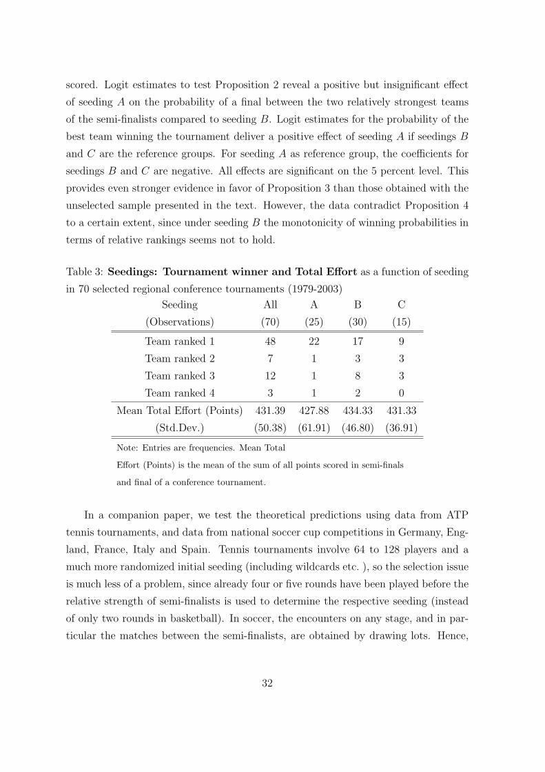
30
on outcomes. If the teams competing in particular seedings are in some way predeter-
mined by the way the 16 teams were seeded initially, the results might be biased: the
teams meeting in semi-finals are selected in a particular way, and hence might differ
systematically with respect to their ability, effort exertion and winning probabilities.
The initial seeding of teams in NCAA basketball tournaments is of type A, i.e. the team
ranked 1 plays team 16 in the first round, and the winner meets the winner of a match
of teams 8 and 9, while in the second bracket the winner of the match between team 2
and team 15 encounters the winner of the match 7-10 etc. This particular seeding has
potential consequences on the possible pairings in semi-finals, since, for example, teams
ranked 1 and 2 can only meet in a regional final, not before. In order to rule out any
potential selection effects resulting from this, we exclude semi-finals between particular
teams that could only happen under certain seedings since teams initially were seeded
according to A. Thus, for example, we exclude any tournament with semi-finals, in
which a team that was absolutely ranked 2 prior to the tournament is the second best
remaining team. Given the initial seeding, this can only happen in semi-final seedings
A and B, but is impossible in seeding C, which requires the highest ranked two teams
meeting in a semi-final. This is impossible due to the initial seeding, so we drop such
a tournament from the sample. On the other hand, a semi-final with team 3 as second
best remaining team is possible under all three seedings given the initial brackets, so
we keep it in the sample.24 This sample selection leads us to drop 30 observations and
leaves us with 70 tournaments with teams in semifinals that have absolute and relative
ranks, which are compatible with any of the three possible seedings, given that the
initial seeding was A. The statistics corresponding to Tables 1 and 2 are depicted in
Tables 3 and 4. Tests of the theoretical predictions using the selected sample deliver
virtually identical, if not somewhat stronger, results than those in the main text ob-
tained from the unselected sample. In particular, the differences in effort as measured
by all points scored are more pronounced and as expected, with seeding B eliciting
the highest effort. However, as with the full sample, the differences are not significant.
The same holds for coefficient estimates of seeding dummies in regressions of all points
24One can easily verify using this argument that the set of teams that have the relatively highest
ability or valuation in the semi-final, which can be obtained under all three seedings is {1, 2, ..., 10},where the numbers are the absolute ranks of teams prior to the tournament; likewise, the set of second-
best teams is {3, ..., 13}, the set of teams relatively ranked 3 is {4, ..., 14}, and the set of weakest teams
is {7, ..., 16}.
31
scored. Logit estimates to test Proposition 2 reveal a positive but insignificant effect
of seeding A on the probability of a final between the two relatively strongest teams
of the semi-finalists compared to seeding B. Logit estimates for the probability of the
best team winning the tournament deliver a positive effect of seeding A if seedings B
and C are the reference groups. For seeding A as reference group, the coefficients for
seedings B and C are negative. All effects are significant on the 5 percent level. This
provides even stronger evidence in favor of Proposition 3 than those obtained with the
unselected sample presented in the text. However, the data contradict Proposition 4
to a certain extent, since under seeding B the monotonicity of winning probabilities in
terms of relative rankings seems not to hold.
Table 3: Seedings: Tournament winner and Total Effort as a function of seeding
in 70 selected regional conference tournaments (1979-2003)
Seeding All A B C
(Observations) (70) (25) (30) (15)
Team ranked 1 48 22 17 9
Team ranked 2 7 1 3 3
Team ranked 3 12 1 8 3
Team ranked 4 3 1 2 0
Mean Total Effort (Points) 431.39 427.88 434.33 431.33
(Std.Dev.) (50.38) (61.91) (46.80) (36.91)
Note: Entries are frequencies. Mean Total
Effort (Points) is the mean of the sum of all points scored in semi-finals
and final of a conference tournament.
In a companion paper, we test the theoretical predictions using data from ATP
tennis tournaments, and data from national soccer cup competitions in Germany, Eng-
land, France, Italy and Spain. Tennis tournaments involve 64 to 128 players and a
much more randomized initial seeding (including wildcards etc. ), so the selection issue
is much less of a problem, since already four or five rounds have been played before the
relative strength of semi-finalists is used to determine the respective seeding (instead
of only two rounds in basketball). In soccer, the encounters on any stage, and in par-
ticular the matches between the semi-finalists, are obtained by drawing lots. Hence,
32
Table 4: Relative Strength of Teams: Composition of Finals and Total Effort
in 70 selected regional conference tournaments (1979-2003)
Composition of Finals Total Points per Match
Match All Seeding A Seeding B Seeding C Mean Std.Dev.
1 vs 2 30 16 14 0 437.63 54.01
1 vs 3 13 8 0 5 427.23 43.14
1 vs 4 13 0 7 6 424.46 59.31
2 vs 3 7 0 4 3 424 38.88
2 vs 4 1 0 0 1 414 .
3 vs 4 6 1 5 0 435.67 53.15
Note: Entries for composition of finals are frequencies.
seedings are completely random, allowing to identify the causal effect of seedings on
effort or winning probabilities without potential selection problems.
33
References
Amegashie, J. (1999): ”The Design of Rent-Seeking Competitions: Committees, pre-
liminary and final Contests”, Public Choice 99, 63-76.
Baye, M. and Kovenock, D. and C. de Vries (1996): ”The All-Pay Auction with
Complete Information”, Economic Theory 8, 291-305.
Baye, M. and Kovenock, D. and C. de Vries (1993): ”Rigging the Lobbying Pro-
cess”, American Economic Review 83, 289-294.
Clark, D. and C. Riis (1998): ”Competition over more than one Prize”, American
Economic Review 88(1), 276-288.
David, H. (1959): ”Tournaments and Paired Comparisons”, Biometrika 46, 139-
149.
Ehrenberg, R. and Bognanno, M. (1990): ”Do Tournaments Have Incentive Ef-
fects?”, Journal of Labor Economics 98, 1307-1324
Glenn, W. (1960): ”A Comparison of the Effectiveness of Tournaments”, Biometrika
47, 253-262.
Gradstein, M. and K.Konrad (1999): ”Orchestrating Rent Seeking Contests”, The
Economic Journal 109, 536-545.
Hillman, A. and J.Riley (1989): ”Politically Contestable Rents and Transfers”,
Economics and Politics 1, 17-40.
Horen, J. and Riezman, R. (1985): ”Comparing Draws for Single Elimination Tour-
naments”, Operations Research 3(2), 249-262.
Hwang, F. (1982): ”New Concepts in Seeding Knockout Tournaments”, American
Mathematical Monthly 89, 235-239
Klaassen, F. and Magnus, J. (2003): ”Forecasting the Winner of a Tennis Match”,
European Journal of Operational Research 148, 257-267.
Rosen, S. (1986): ”Prizes and Incentives in Elimination Tournaments”, American
Economic Review 74, 701-715.
34
Searles, D. (1963): ”On the Probability of Winning with Different Tournament
Procedures”, Journal of the American Statistical Association 58, 1064-1081.
Schwenk, A. (2000): ”What is the Correct Way to Seed a Knockout Tournament”,
American Mathematical Monthly 107, 140-150
USA Today (2003): ”Weighted Brackets in NCAA draw fire”, March 26.


![VE1-3.PPT [Schreibgeschützt] [Kompatibilitätsmodus] · Toxikokinetik • Resorption (Aufnahme) • Verteilung • Metabolismus (Biotransformation) • Elimination (Ausscheidung)](https://static.unterlagen.site/doc/80x56/5d4f197688c9932e758b9f6e/ve1-3ppt-schreibgeschuetzt-kompatibilitaetsmodus-toxikokinetik-resorption.jpg)
