177
Dominik Joho Learning and Utilizing Spatial Object Relations for Service Robots

Dominik Joho
Learning and UtilizingSpatial Object Relations
for Service Robots

Learning and UtilizingSpatial Object Relationsfor Service Robots
Dominik Joho
Dissertation zur Erlangung des akademischen Grades Doktor der NaturwissenschaftenTechnische Fakultät, Albert-Ludwigs-Universität Freiburg
Dekan Prof. Dr. Yiannos ManoliErstgutachter Prof. Dr. Wolfram Burgard
Albert-Ludwigs-Universität FreiburgZweitgutachter Prof. Dr. Bernhard Nebel
Albert-Ludwigs-Universität FreiburgTag der Disputation 10. Dezember 2013

Abstract
Service robots that operate in domestic environments and assist in the daily housework arestill beyond reach when considering the current state of the art. Hence, they pose many inte-resting technical challenges that currently motivate a considerable amount of basic researchin mobile robotics. One of these challenges is the question how service robots could attainthe required level of autonomy and reliability to be truly useful. Ideally, if a service robotis deployed in a domestic environment it should require only a short setup time and as fewuser interactions as possible. When tidying up, it should know where the objects usuallybelong to. If the robot should set the table, it needs to know which objects are required,where to find them, and how they should be arranged on the table. It is apparent that mostof these tasks involve knowledge about the spatial context of objects and how objects areusually arranged in such environments. It would be desirable to have a flexible approach inwhich the robot adapts to the specifics of its environment by observing it. It thereby couldlearn the usual object arrangements. Hence, as a basic requirement for achieving a highlevel of autonomy, service robots need to represent, learn, and utilize knowledge about therelevant spatial relations between objects in man-made environments. If robots are able toutilize representations that take into account the interdependencies between objects in suchenvironments then this would enable them to more efficiently carry out their tasks or to ad-dress completely new tasks. For example, robots could more efficiently search for objects,or a robot could reason about missing or misplaced objects in a room or on a table.
In this thesis, we propose several techniques for learning and utilizing spatial object rela-tions. First, we consider the problem of localizing objects. As future household objects andretail products might be equipped with an RFID tag, we first present a technique to localizeRFID tags. Further, we show that same technique can also be applied to the complementarysituation in which we want to localize a mobile robot based on a known map of RFID taglocations. Given that we can localize objects, we move on to address the question of howa robot can efficiently search for objects in an unknown environment. For this, we presenttwo techniques that both aim at speeding up the search process by taking advantage of back-ground knowledge about usual object arrangements acquired in previously seen, similarlystructured environments. Specifically, we are interested in efficiently finding a product in anunknown supermarket. The main idea is to exploit knowledge about the co-occurrence of
vi
objects to focus on searching the promising regions first and to postpone the non-promisingregions. While both approaches utilize learning techniques to leverage the information ofpreviously seen environments, they both rely on predefined spatial relations, like an objectbeing “in the same aisle” as another object. This motivates the final part of this thesis, inwhich we aim at learning stable spatial relations between objects. More specifically, wewish to learn spatially coherent object constellations in an unsupervised manner from com-plex multi-object scenes. As an application scenario, we consider tabletop scenes in whichthe object constellations correspond to place covers. For this, we propose a novel hierarchi-cal nonparametric Bayesian model that represents a prior distribution over scene structuresin terms of object constellations. For posterior inference in this model, we present an effi-cient Markov chain Monte Carlo (MCMC) sampler. By basing our model on the Dirichletprocess and the beta-Bernoulli process, the number of object constellations in our modelis not fixed. This has practical benefits in the context of lifelong learning, as the robot isable to recognize and integrate previously unseen object constellations into its model in anopen-ended fashion and within a single coherent probabilistic framework.
Zusammenfassung
Serviceroboter, die bei der täglichen Hausarbeit helfen, die das Geschirr abwaschen, ein-kaufen, aufräumen und den Tisch decken, sind noch weit jenseits der heutigen technischenMöglichkeiten. Sie stellen damit aber auch eine interessante technische Herausforderungdar und motivieren derzeit einen guten Anteil der Grundlagenforschung in der mobilen Ro-botik. Eine jener Herausforderungen ist die Frage, wie Serviceroboter das notwendige Maßan Autonomie und Verlässlichkeit erreichen können, um wirklich nützlich zu sein. Idealer-weise sollte ein Roboter, sobald er in einer neuen Umgebung eingesetzt wird, eine mög-lichst geringe Einrichtezeit benötigen und dabei auf so wenig Benutzerinteraktionen wiemöglich angewiesen sein. Das heißt, um das Geschirr zu waschen, sollte er das Geschirrund die Küche selbständig finden. Um aufzuräumen, muss er wissen, wohin die Gegen-stände gehören. Um den Tisch zu decken, muss er wissen, welche Gegenstände benötigtwerden, wo sie zu finden sind, und wie sie auf dem Tisch zu arrangieren sind.
Es ist offensichtlich, dass die meisten dieser Aufgaben Vorwissen über den räumlichenKontext von Objekten erfordert. Zum Beispiel muss klar sein, wie Objekte in solchen Um-gebungen normalerweise arrangiert sind. Der Benutzer könnte dem Roboter in einer Ein-arbeitungsphase dieses Wissen vermitteln, oder der Roboter wird mit einprogrammiertenVorwissen ausgeliefert, das es ihm z. B. ermöglicht, einen Tisch zu decken. Beide Mög-lichkeiten erscheinen jedoch unbefriedigend. Während eine Einarbeitungsphase zeitinten-siv sein kann, ist einprogrammiertes Vorwissen unflexibel, wenn es sich nicht an die Wün-sche des Nutzers anpassen lässt. Es wäre daher erstrebenswert, einen flexibleren Ansatz zuverfolgen, bei dem der Roboter sich an die Spezifika seiner Umgebung selbst anpasst. Da-durch wäre es ihm möglich, die Objektarrangements und relevanten Objektrelationen selbstdurch Beobachtung seiner Umgebung zu lernen.
Als Grundvoraussetzung um wirklich nützlich zu sein und einen hohen Grad an Autono-mie zu erreichen, sollte ein Serviceroboter daher Vorwissen über die relevanten räumlichenObjektrelationen repräsentieren, erlernen und einsetzen können. Wenn Roboter in der Lagewären, auf Repräsentationen zurückzugreifen, welche die wechselseitigen Abhängigkeitenzwischen Objekten berücksichtigen, würde sie dies dazu befähigen, ihre Aufgaben effizien-ter auszuführen, oder komplett neuartige Aufgaben zu erledigen. Beispielsweise könnte einRoboter effizienter nach Objekten suchen, indem er sich zunächst auf die vielversprechen-
viii
den Regionen konzentriert. Ob eine Region dabei als vielversprechend angesehen wird,sollte hauptsächlich davon abhängen, welche anderen Gegenstände dort bereits erkanntwurden, sowie der Wahrscheinlichkeit, dass der gesuchte Gegenstand zusammen mit diesenGegenständen auftritt. Zudem könnte ein Roboter mittels solcher Repräsentationen fehlen-de oder deplatzierte Objekte in einem Raum oder auf einem Tisch erkennen. So könnte derRoboter über die Zeit eine Repräsentation der Gedecke auf einem Frühstückstisch gelernthaben. Dies würde es ihm ermöglichen, die Struktur eines teilweise gedeckten Tisches zuanalysieren, die fehlenden Objekte zu identifizieren und dem Menschen beim Decken desTisches zu assistieren.
In der vorliegenden Dissertation präsentieren wir verschiedene Techniken als erste Schrit-te in Richtung des langfristigen Ziels der Realisierung eines autonomen Serviceroboters.Zunächst sollte der Roboter in der Lage sein, Objekte zu erkennen. Da zukünftige Haus-haltsgegenstände und Produkte bereits mit einem RFID-Etikett versehen sein könnten,schlagen wir eine Methode zur Lokalisierung dieser Objekte auf Basis der RFID-Technikvor. Um die Position der RFID-Etiketten zu bestimmen, verwenden wir eine RFID-Antenne,die auf einer mobilen Sensorplattform oder einem mobilen Roboter montiert ist. Mittels die-ser Antenne kann die eindeutige ID der RFID-Etiketten ausgelesen werden. Zudem wirddabei jeweils die Signalstärke gemessen, mit der diese Information empfangen wurde. Dervon uns vorgeschlagene Ansatz ist in der Lage, diese Messungen zu einer Wahrschein-lichkeitsverteilung über die Position eines Etiketts zu integrieren. Zudem ist unser An-satz für die komplementäre Situation einsetzbar, in der die Positionen der RFID-Etikettenbekannt sind und auf Basis der Messungen die Trajektorie des Roboters geschätzt wer-den soll. In beiden Situationen ist unser Ansatz jedoch auf ein probabilistisches Sensor-modell angewiesen, das einen Bezug zwischen der Roboter- und Etikettposition und dererhaltenen Messung herstellt. Ein Hauptbeitrag unseres Ansatzes ist daher ein neuartigesprobabilistisches Sensormodell für die RFID-basierte Lokalisierung, das im Gegensatz zufrüheren Ansätzen sowohl die empfangene Signalstärke berücksichtigt, als auch die De-tektionswahrscheinlichkeit modelliert. In unseren Experimenten zeigen wir, dass dies einegenauere Positionsschätzung erlaubt, als dies durch ein Sensormodell möglich wäre, dasnur die Signalstärke oder nur Detektionsereignisse berücksichtigt. Der zusätzlich zu veran-schlagende Berechnungsaufwand, der benötigt wird, um beide Modalitäten zu berücksich-tigen, ist vernachlässigbar. Das von uns vorgeschlagene Sensormodell fällt in die Kategorieder antennenzentrischen Sensormodelle, welche die erwarteten Messungen in einem Be-zugssystem relativ zur Antenne modellieren. Die Kalibrierung solcher Modelle kann rechtaufwendig sein. Es müssen Referenzmessungen an verschiedenen antennenrelativen Posi-
ix
tionen vorgenommen werden. Dazu kann einerseits die Antenne fix gehalten werden undvon einem RFID-Etikett an verschiedenen relativen Positionen Messungen vorgenommenwerden. Andererseits könnte man verschiedene Etiketten in der Umgebung verteilen undeine lokalisierte Antenne durch diese Umgebung bewegen. Da sowohl Antennenpositionals auch Etikettpositionen bekannt sind, können die Messungen in ein antennenzentrischesBezugssystem zurückgerechnet werden. Ein großer Nachteil beider Methoden ist jedoch,dass die Positionen der RFID-Etiketten bekannt sein müssen. Wir stellen deshalb ein Ver-fahren vor, das diese Kalibrierungsphase dahingehend vereinfacht, dass im Vorfeld keineEtikettpositionen ermittelt werden müssen. Dies wird durch ein iteratives Verfahren er-reicht, das sowohl das Sensormodell als auch die Etikettpositionen schätzt. In Experimentenzeigen wir, dass das so gelernte Sensormodell gegen ein nicht-iterativ gelerntes Sensormo-dell konvergiert (bis auf einen gewissen empirischen Fehler). Dabei ist das nicht-iterativeVerfahren weiterhin auf bekannte Etikettpositionen angewiesen. Zudem zeigen unsere Er-gebnisse, dass die im iterativen Verfahren simultan geschätzten Etikettpositionen gegendie tatsächlichen Positionen konvergieren (bis auf einen gewissen empirischen Fehler). Wirmöchten betonen, dass das iterative Verfahren nur notwendig ist, sofern die Annahme fallengelassen werden soll, dass die Etikettpositionen bekannt seien. Wir werden unser Verfah-ren und Varianten davon quantitativ in einem Büro und einem Supermarkt evaluieren. Diesschließt einen Vergleich mit aus der Literatur bekannten Methoden ein. Dazu implementie-ren wir eine WiFi-basierte Lokalisierungsmethode, die eine 2D-Signalstärkekarte mittelsGauß-Prozess-Regression schätzt. Zudem adaptieren wir das Modell, sodass die Signal-stärke auch im Posenraum kartiert werden kann. Dies ist besonders für die RFID-basierteLokalisierung relevant, da die empfangene Signalstärke in erheblichen Maß von der Orien-tierung der Antenne abhängt.
Im Folgenden wollen wir nun annehmen, dass der Roboter in der Lage ist, Objekte zulokalisieren. Wir wenden uns dann der Frage zu, wie er Hintergrundwissen über gebräuch-liche Objektarrangements ausnutzen kann, um seine Aufgaben effizienter auszuführen, ins-besondere, wenn er Objekte in einer unbekannten Umgebung sucht. Zur Motivation ver-anschaulichen wir uns die Situation, dass wir ein bestimmtes Produkt in einem unbekann-ten Supermarkt suchen. Sicher würden wir nicht einfach zufällig durch den Markt gehen,aber genauso wenig würden wir systematisch jeden einzelnen Gang ablaufen bis wir dasProdukt finden. Vielmehr würden wir unser Suchverhalten von unseren aktuellen Beobach-tungen abhängig machen, sowie von unserem Vorwissen darüber, wie Objekte in solchenUmgebungen üblicherweise angeordnet sind. Dieses Vorwissen basiert auf unseren Erfah-rungen in anderen Supermärkten, in denen uns gewisse stabile räumliche Abhängigkeiten
x
zwischen Produktgruppen aufgefallen sind. Die Aufgabe ist nun, dieses Wissen zunächstin einer geeigneten Weise zu formalisieren, sodass ein Roboter dies ebenfalls auf Basis vonDaten echter Supermärkte erlernen kann. Zudem müssen wir eine Suchstrategie entwerfen,die dieses Wissen für eine effiziente Suche ausnutzen kann.
Wir stellen dafür zwei alternative Ansätze vor. Unser erster Ansatz ist eine reaktive Such-strategie, welche die Entscheidung, wo als nächstes gesucht werden soll, von den aktuelldirekt sichtbaren Objekten der näheren Umgebung abhängig macht. Als Suchheuristik ver-wendet der Roboter dabei Entscheidungsbäume, welche die Alternativen an einer Wegga-belung in einem Supermarkt in vielversprechende und weniger aussichtsreiche Richtun-gen klassifiziert. Die Entscheidungsbäume werden auf Daten von optimalen Suchpfaden inTrainingsmärkten gelernt. Im Gegensatz dazu verfolgt unsere zweite Suchstrategie einenglobaleren, inferenzbasierten Ansatz, der alle bisher gesehenen Objekte und Strukturen imSupermarkt berücksichtigt. Auf Basis dieser Beobachtungen wird eine Verteilung über diemögliche Position des Produkts berechnet. Der Roboter wählt dann einen Zielpunkt aus,indem er die Distanz zu diesem Zielpunkt mit der Wahrscheinlichkeit abwägt, das Produktan diesem Ort zu finden. Er führt dann seine Suche fort, indem er sich auf dem kürzestenWeg zu diesem Zielpunkt begibt. Sobald neue Informationen zur Verfügung stehen, d.h.neue Produkte oder Strukturen gesehen werden, wird die Verteilung neu berechnet und einneuer Zielpunkt ausgewählt. Die Verteilung basiert auf einem Modell, das im Grunde dieWahrscheinlichkeit berücksichtigt, dass zwei Objekte in bestimmten räumlichen Kontextengemeinsam auftreten. Die Parameter dieses Modells können auf Basis von Karten von Su-permärkten gelernt werden. Zwar unterscheiden sich beide Suchstrategien in ihren techni-schen Details, sie werden jedoch beide auf einer Trainingsmenge von drei Märkten trainiertund in einem vierten Supermarkt evaluiert. Die benötigten Daten wurden in vier echten Su-permärkten erhoben und modellieren im Detail die Regalaufstellungen und die Platzierungder Produkte. Die Effizienz beider Suchstrategien vergleichen wir quantitativ mit einer Ba-sisstrategie, die den Markt erkundet bis das Produkt gefunden wird. Zudem präsentieren wireinen Vergleich zum Abschneiden von Versuchspersonen die in einer Feldstudie in einemechten Supermarkt nach den gleichen Produkten suchen mussten.
Die inferenzbasierte Suchstrategie nutzt Kookkurrenz-Statistiken über Objekte in ver-schiedenen räumlichen Kontexten. Z. B. wird die Wahrscheinlichkeit betrachtet, dass dasgesuchte Produkt sich “im gleichen Regal” oder “in einem benachbarten Regal” befindenkönnte, wie ein anderes, während der Suche bereits gesehenes Produkt. Zwar können dieParameter des Modells auf Basis von Karten von Supermärkten gelernt werden, die da-bei betrachteten räumlichen Relationen sind jedoch vordefiniert und werden nicht gelernt.
xi
Deshalb wenden wir uns in unserem letzten Beitrag dieser Arbeit einem allgemeinerenLernszenario zu, in dem wir den räumlichen Kontext von Objekten lernen wollen. Konkretwollen wir unüberwacht räumlich stabile Objektkonstellationen in komplexen Alltagssze-nen lernen. Als Anwendungsszenario betrachten wir Tischszenen in denen die relevantenObjektkonstellationen den Gedecken entsprechen, die, z. B., aus den Objekten Teller, Mes-ser und Kaffeetasse bestehen. Die Identifikation von relevanten Objektkonstellationen kannals Parsen der Szene oder als Inferenz der unbekannten Szenenstruktur angesehen werden.Für eine gegebene Szene existieren jedoch im Allgemeinen verschiedene mögliche Inter-pretationen ihrer Struktur. Eine Szene kann als Ansammlung zufällig verteilter Objekteangesehen werden, oder sie kann als ganzes als eine einzige, große Objektkonstellation in-terpretiert werden. Für die Szene eines Frühstückstisches, der für drei Personen gedecktist, würden wir es jedoch als viel wahrscheinlicher ansehen, dass drei sich wiederholendeObjektkonstellationen zu finden sind – eben die Gedecke. Wir werden den Begriff einer“wahrscheinlicheren Szenenstruktur” präzisieren, indem wir eine a-priori-Verteilung überSzenenstrukturen definieren. Diese Verteilung könnte dann zur Evaluation der Wahrschein-lichkeiten der oben genannten alternativen Szenenbeschreibungen herangezogen werden.Zudem kann diese Verteilung aktualisiert werden und somit eine a-posteriori-Verteilungüber Szenenstrukturen modellieren, die Informationen über bereits analysierte Szenen mit-einbezieht. Wenn ein Roboter noch nie eine Frühstücksszene gesehen hat, könnte er die dreigenannten alternativen Szenenstrukturen als mehr oder weniger gleich wahrscheinlich an-sehen. Hätte er jedoch bereits mehrere Szenen analysiert, in denen ähnliche Objektkonstel-lationen auftreten, würde er eher mit unserer Intuition übereinstimmen, dass ein Frühstück-stisch für drei Personen drei relevante Konstellationen enthält die gerade den Gedeckenentsprechen.
Konkret besteht unser Beitrag in der Definition eines neuen, hierarchischen, nicht-pa-rametrischen Bayes’schen Modells für komplexe Szenen die aus mehreren Objekten auf-gebaut sind. Ein grundlegender Baustein unseres Modells sind sogenannte Meta-Objekte,die eine Verteilung über Objektkonstellationen definieren. Wir nehmen an, dass die Ob-jektkonstellationen auf einem Tisch aus diesen Meta-Objekten gesampelt wurden. Meta-Objekte sind als probabilistische, teilbasierte Modelle definiert und besitzen damit eineinterne Struktur. Ein “Teil” eines solchen Modells, beinhaltet (a) eine räumliche Vertei-lung, welche die relative Position des Objekts festlegt, (b) eine kategoriale Verteilung,welche den Typ des Objekts festlegt, das auf diese relative Position gestellt werden soll(Teller, Tasse, etc.) und (c) eine Aktivierungswahrscheinlichkeit, welche festlegt, ob über-haupt ein Objekt auf diese Position zu stellen ist. Ein Meta-Objekt in einer Frühstücksszene
xii
könnte z. B. aus vier Teilen bestehen: einem “zentralen Teil”, mit einer hohen Wahrschein-lichkeit für Teller, einem “linken Teil”, mit einer hohen Wahrscheinlichkeit für Gabeln,etc. Um eine Objektkonstellation aus diesem Modell zu sampeln, wird zunächst die Ak-tivierung der Teile gesampelt. Für jeden aktivierten Teil sampeln wir die relative Positionund den Objekttyp. Dadurch generiert jeder Teil eines solchen Modells höchstens ein Ob-jekt. Die Objektkonstellation wird dann in die Szene transformiert, indem wir aus einera-priori-Verteilung über Transformationen sampeln. Wir nehmen an, dass eine Szene ausmehreren Objektkonstellationen bestehen kann. Zudem nehmen wir an, dass verschiedeneKategorien von Konstellationen existieren, mit jeweils unterschiedlichen Parametrisierun-gen für die Wahrscheinlichkeitsverteilungen ihrer Teile. So könnte eine bestimmte Meta-Objektkategorie mit hoher Wahrscheinlichkeit eine Müslischale und einen Löffel sampeln,während eine andere Kategorie eher Konstellationen mit Teller und Messer sampelt. EineSzene zu analysieren, heißt, diesen generativen Prozess umzukehren, indem die Anzahl derObjektkonstellationen, deren jeweilige Kategorie und ihre zugehörige Transformation oderReferenzrahmen inferiert werden. Zudem muss jedes Objekt zu einer bestimmten Meta-Objektinstanz assoziiert werden, sowie zu einem bestimmten Teil dieser Instanz. So sollteetwa ein Teller mit dem zentralen Teil eines Meta-Objekts assoziiert werden.
Bisher haben wir noch nicht die Anzahl an Kategorien von Meta-Objekten oder die An-zahl der Teile pro Meta-Objekt-Kategorie in unserem Modell festgelegt. Es wäre wün-schenswert, eine genaue Spezifikation dieser Zahlen zu vermeiden, und sie stattdessenaus den Daten zu schätzen. Dies erreichen wir dadurch, dass unser Modell als nicht-para-metrisches Bayes’sches Modell auf Basis des Dirichlet-Prozesses und des Beta-Bernoulli-Prozesses definiert wird. Hiermit vermeiden wir sogar, eine Obergrenze für diese Zahlenangeben zu müssen. Stattdessen entspricht dies der Annahme, dass es unendlich viele Ka-tegorien von Meta-Objekten gibt, die jeweils unendlich viele Teile besitzen. Dies bedeutet,dass nun die effektive Anzahl der Meta-Objekt-Kategorien und -Teile ebenfalls aus denDaten inferiert wird. In unserem Modell können wir nun gewisse Hyperparameter setzen,die unsere a-priori Vorstellungen über diese Zahlen widerspiegeln. Dies eröffnet die Mög-lichkeit, aus den Daten die effektive Modellkomplexität zu inferieren, die sich somit derDatenkomplexität anpassen kann. Dies hat für den Roboter auch praktische Konsequen-zen für Szenarien des lebenslangen Lernens. Da die Anzahl der Objektkonstellationen inunserem Modell variabel gehalten ist, kann der Roboter neue, bisher noch nie gesehene Ob-jektkonstellationen als solche erkennen und in sein Modell integrieren – und dies innerhalbeines einzigen, kohärenten probabilistischen Rahmens.

Acknowledgements
A doctoral thesis is the work of a single one, but it is well understood that such a project isimpossible without the guidance and support of colleagues and friends. I am indebted to afew people and I want to take the opportunity to thank them here.
First of all, I want to thank Prof. Dr. Wolfram Burgard for giving me the opportunity towork in his group. He gave me considerable freedom to pursue my own interests and I amgrateful for this and the trust that this implies. The mindset to approach technical problemsfrom a probabilistic point of view is considered by me to be the most important lesson thatI have learned in these years and I attribute this mainly to his influence.
I also want to thank Prof. Dr. Bernhard Nebel for acting as a second referee.
The stimulating and motivating atmosphere at the AIS lab certainly had a great influenceon this thesis. There are now so many people working in the lab that I refrain from namingeveryone individually. Each one contributed his or her share in creating this atmosphereand every one deserves my gratitude for that. And at times, the AIS lab was more thanjust a workplace. I especially remember our stay in Kobe and Osaka during ICRA’09 as anoutstanding experience.
I really enjoyed the inspiring discussions with Dr. Gian Diego Tipaldi during our workon the scene analysis paper. He supported me in trying out my own ideas, but he also tookcare to point out to me the things that might not work – and this is perhaps one of the bestways of supervising someone. Especially, he convinced me that my favorite toy from thelast paper would likely be of no use for the current problem. So I started looking for a newtoy. And I think this was a crucial step.
Further, I want to thank Dr. Christian Plagemann for the collaboration during our workon the RFID paper. He helped me to understand the idea of Gaussian process regression andhe also kindly gave me access to his own implementation for Gaussian process regression.
I want to thank Dagmar Sonntag and Susanne Bourjaillat for administrative support, andMichael Keser for technical support. I also thank Martin Senk for the collaboration duringhis Bachelor’s thesis, especially, for the additional work he has done for the conference andjournal paper. Further, I thank Nikolas Engelhard for implementing the segmentation andclassification of the point clouds for the scene analysis paper.
I also collaborated with Christopher Kalff when we used the RFID localization technique

xiv
to track the participants in a field study that he conducted in a supermarket. In turn, he pro-vided me with an evaluation of the resulting trajectories, which enabled me to comparethe performance of my search technique to the performance of the human subjects (unfor-tunately, the humans won). I think, this was an interesting addition to one of my papers.Sadly, it is too late now to thank him for this collaboration at this point.
I thank Dr. Barbara Frank, Dr. Zeno Gantner, Markus Kuderer, PD Dr. Cyrill Stachniss,Dr. Gian Diego Tipaldi, and Dr. Thorsten Zitterell for reading parts of an earlier version ofthis thesis.
Finally and most importantly, I want to thank my wife Karla Alcázar for the support andlove throughout these years. She always believed in me and this thesis would not have beenpossible without her. And hats off to our son Julian, for his proficiency in destroying anymeaningful object arrangement in our very own domestic environment on a daily basis.
This work has been supported by the Deutsche Forschungsgemeinschaft (DFG) under contract number SFB/TR 8
Spatial Cognition (R6-[SpaceGuide]).

Para Karla y Julian.

Contents
1 Introduction 11.1 Contributions . . . . . . . . . . . . . . . . . . . . . . . . . . . . . . . . . 8
1.1.1 RFID-based Localization and Mapping . . . . . . . . . . . . . . . 81.1.2 Object Search in Unknown Environments . . . . . . . . . . . . . . 91.1.3 Scene Analysis . . . . . . . . . . . . . . . . . . . . . . . . . . . . 9
1.2 Publications . . . . . . . . . . . . . . . . . . . . . . . . . . . . . . . . . . 101.3 Collaborations . . . . . . . . . . . . . . . . . . . . . . . . . . . . . . . . . 111.4 Notation . . . . . . . . . . . . . . . . . . . . . . . . . . . . . . . . . . . . 12
2 Basics 132.1 Basics of Probability Theory . . . . . . . . . . . . . . . . . . . . . . . . . 142.2 Monte Carlo Methods . . . . . . . . . . . . . . . . . . . . . . . . . . . . . 18
2.2.1 Importance Sampling . . . . . . . . . . . . . . . . . . . . . . . . . 182.2.2 Markov Chain Monte Carlo . . . . . . . . . . . . . . . . . . . . . 202.2.3 Monte Carlo Localization for Mobile Robots . . . . . . . . . . . . 22
2.3 Decision Tree Learning . . . . . . . . . . . . . . . . . . . . . . . . . . . . 252.4 Maximum Entropy Models . . . . . . . . . . . . . . . . . . . . . . . . . . 262.5 Bayesian Nonparametrics . . . . . . . . . . . . . . . . . . . . . . . . . . . 30
2.5.1 Dirichlet Process and Chinese Restaurant Process . . . . . . . . . . 302.5.1.1 Finite Gaussian Mixture Models . . . . . . . . . . . . . 312.5.1.2 Dirichlet Process Gaussian Mixture Models . . . . . . . 352.5.1.3 Definition of the Dirichlet Process . . . . . . . . . . . . 382.5.1.4 Stick-breaking Construction . . . . . . . . . . . . . . . . 382.5.1.5 Chinese Restaurant Process . . . . . . . . . . . . . . . . 402.5.1.6 Dirichlet Process Gaussian Mixture Models Revisited . . 41
2.5.2 Beta-Bernoulli Process and Indian Buffet Process . . . . . . . . . . 422.5.3 Hierarchical Processes . . . . . . . . . . . . . . . . . . . . . . . . 462.5.4 Nested Processes . . . . . . . . . . . . . . . . . . . . . . . . . . . 482.5.5 Gaussian Process Regression . . . . . . . . . . . . . . . . . . . . . 50
xviii Contents
3 RFID-based Object Localization and Self-Localization 533.1 The Sensor Model . . . . . . . . . . . . . . . . . . . . . . . . . . . . . . . 54
3.2 Learning the Model from Data . . . . . . . . . . . . . . . . . . . . . . . . 57
3.2.1 Semi-Autonomous Learning . . . . . . . . . . . . . . . . . . . . . 57
3.2.2 Bootstrapping the Sensor Model . . . . . . . . . . . . . . . . . . . 57
3.3 Mapping Tags from Known Sensor Poses . . . . . . . . . . . . . . . . . . 58
3.4 Localizing a Mobile Agent . . . . . . . . . . . . . . . . . . . . . . . . . . 60
3.5 Experimental Evaluation . . . . . . . . . . . . . . . . . . . . . . . . . . . 63
3.5.1 Localizing the RFID Tags . . . . . . . . . . . . . . . . . . . . . . 64
3.5.2 Localizing a Mobile Agent . . . . . . . . . . . . . . . . . . . . . . 64
3.6 Future Work . . . . . . . . . . . . . . . . . . . . . . . . . . . . . . . . . . 68
3.7 Related Work . . . . . . . . . . . . . . . . . . . . . . . . . . . . . . . . . 68
3.8 Conclusions . . . . . . . . . . . . . . . . . . . . . . . . . . . . . . . . . . 69
4 Searching for Objects 714.1 Reactive Search Strategy . . . . . . . . . . . . . . . . . . . . . . . . . . . 74
4.1.1 Modeling the Environment . . . . . . . . . . . . . . . . . . . . . . 74
4.1.2 Learning Search Heuristics . . . . . . . . . . . . . . . . . . . . . . 76
4.1.2.1 Defining Edge Attributes . . . . . . . . . . . . . . . . . 76
4.1.2.2 Generating Training Data . . . . . . . . . . . . . . . . . 78
4.1.2.3 Decision Tree Learning and Pruning . . . . . . . . . . . 80
4.1.3 Variants of the Decision Tree Strategy . . . . . . . . . . . . . . . . 80
4.2 Inference-based Search Strategy . . . . . . . . . . . . . . . . . . . . . . . 81
4.2.1 Modeling the Evironment . . . . . . . . . . . . . . . . . . . . . . 81
4.2.2 A Model for Inferring Object Locations . . . . . . . . . . . . . . . 83
4.2.2.1 Application to the Supermarket Scenario . . . . . . . . . 88
4.2.3 Selecting a Target Location . . . . . . . . . . . . . . . . . . . . . . 90
4.3 Experimental Evaluation . . . . . . . . . . . . . . . . . . . . . . . . . . . 91
4.3.1 Evaluation in Comparison to Humans . . . . . . . . . . . . . . . . 92
4.3.2 Evaluation with Varying Starting Locations . . . . . . . . . . . . . 95
4.3.3 Reactive Search Strategy – Searching with a Real Robot . . . . . . 97
4.3.4 Inference-based Search Strategy – Further Evaluations . . . . . . . 101
4.4 Related Work . . . . . . . . . . . . . . . . . . . . . . . . . . . . . . . . . 103
4.5 Conclusions . . . . . . . . . . . . . . . . . . . . . . . . . . . . . . . . . . 105

Contents xix
5 Unsupervised Learning of Object Constellations 1075.1 Generative Scene Model . . . . . . . . . . . . . . . . . . . . . . . . . . . 110
5.1.1 Description of the Generative Process . . . . . . . . . . . . . . . . 1105.1.2 Posterior Inference in the Model . . . . . . . . . . . . . . . . . . . 114
5.1.2.1 Joint Distribution . . . . . . . . . . . . . . . . . . . . . 1155.1.2.2 Death (Birth) Move . . . . . . . . . . . . . . . . . . . . 1175.1.2.3 Switch Move . . . . . . . . . . . . . . . . . . . . . . . . 1185.1.2.4 Shift Move . . . . . . . . . . . . . . . . . . . . . . . . . 1195.1.2.5 Association Move (Existing Part) . . . . . . . . . . . . . 1195.1.2.6 Association Move (New Parts) . . . . . . . . . . . . . . 1195.1.2.7 Birth Proposal . . . . . . . . . . . . . . . . . . . . . . . 120
5.2 Experiments . . . . . . . . . . . . . . . . . . . . . . . . . . . . . . . . . . 1215.2.1 Synthetic Data . . . . . . . . . . . . . . . . . . . . . . . . . . . . 1215.2.2 Real-world Data . . . . . . . . . . . . . . . . . . . . . . . . . . . 122
5.3 Related Work . . . . . . . . . . . . . . . . . . . . . . . . . . . . . . . . . 1245.4 Conclusion . . . . . . . . . . . . . . . . . . . . . . . . . . . . . . . . . . 127
6 Discussion 1296.1 Outlook . . . . . . . . . . . . . . . . . . . . . . . . . . . . . . . . . . . . 132
6.1.1 RFID-based Object Localization and Self-Localization . . . . . . . 1326.1.2 Searching for Objects . . . . . . . . . . . . . . . . . . . . . . . . . 1336.1.3 Learning Object Constellations . . . . . . . . . . . . . . . . . . . . 134
6.2 Concluding Remarks . . . . . . . . . . . . . . . . . . . . . . . . . . . . . 136
A Appendix 139A.1 Posterior Predictive Distribtion w.r.t. a Normal-Wishart Prior . . . . . . . . 139A.2 Derivations for the MaxEnt Model (Part 1) . . . . . . . . . . . . . . . . . . 140A.3 Derivations for the MaxEnt Model (Part 2) . . . . . . . . . . . . . . . . . . 142


CHAPTER 1
Introduction
Service robots that operate in domestic environments and assist in the daily housework,that wash the dishes, go shopping, tidy up, and set the table, are still beyond reach whenconsidering the current state of the art. Hence, they pose many interesting technical chal-lenges that currently motivate a considerable amount of basic research in mobile robotics.One of these challenges is the question how service robots could attain the required levelof autonomy and reliability to be truly useful. Ideally, if a service robot is deployed in adomestic environment it should require only a short setup time and as few user interactionsas possible. That is, for washing the dishes it should find and recognize the plates andthe kitchen sink by itself instead of being manually instructed. When tidying up, it shouldknow where the objects usually belong to. If the robot should set the table, it needs to knowwhich objects are required, where to find them, and how they should be arranged on thetable.
It is apparent that most of these tasks involve knowledge about the spatial context ofobjects and how objects are usually arranged in such environments. Hence, the user couldeither go through a lengthy instruction phase in which he or she directly demonstrates thesetasks to the robot, or the robot could have pre-programmed knowledge about how to, for ex-ample, set a table. Both options seem unsatisfactory as the first approach is time-consumingand the latter ignores the preferences of the user. Therefore, it would be desirable to havea more flexible approach in which the robot adapts to the specifics of its environment byobserving it. Thereby, it could learn the usual object arrangements and relevant spatialrelations between objects.
Thus, as a basic requirement for being truly useful and for achieving a high level of au-tonomy, service robots need to represent, learn, and utilize knowledge about the relevant
2 Chapter 1 Introduction
spatial relations between objects in man-made environments. If robots are able to utilizerepresentations that take into account the interdependencies between objects in man-madeenvironments then this would enable them to more efficiently carry out their tasks or toaddress completely new tasks that would have been impossible without such representa-tions. For example, robots could more efficiently search for objects by first searching thepromising regions and postponing the non-promising regions. If a regions looks promisingor not will mainly depend on the objects the robots sees there as well as its prior knowledgeabout how likely the sought object co-occurs with these objects. Further, a robot couldreason about missing or misplaced objects in a room or on a table. For example, over timethe robot might have learned a representation of the layout of covers on a breakfast table.Based on this, it could parse a partially laid table, identify the missing objects, and aid thehuman with setting the table.
In this thesis, we present several techniques as preliminary steps towards the long-termgoal of building autonomous service robots. First, a robot obviously must be able to detectand localize the objects in the first place. As future household objects and retail productsmight already be equipped with RFID tags, we therefore present a novel approach to RFID-based localization and mapping. The location of RFID tags can be estimated by means ofan RFID antenna attached to a localized sensor platform or robot. While moving throughthe environment, the robot collects measurements of the RFID tags that include the sig-nal strength as well as the unique ID of a tag. The measurements are then integrated tocompute a distribution over the location of each RFID tag. Further, the approach can alsobe used for the complementary situation in which we are given a map of RFID tag loca-tions and the task is to estimate the trajectory of a robot moving through this environment.Both of these tasks rely on a sensor model that relates the robot and tag locations to themeasurements. Hence, we propose a novel probabilistic sensor model that, in contrast topreviously published approaches, explicitly considers both tag detection events as well asthe received signal strength in a combined model. Our experiments show that this leads toan improved localization accuracy when compared to sensor models that utilize either onlythe signal strength or only tag detection events. The additional computational overhead forconsidering both is negligible. Our proposed sensor model belongs to the class of antenna-centric sensor models, which represent the expected measurements in an antenna-relativeframe of reference. The calibration phase for such models can be quite tedious. One needsto obtain reference measurements at several antenna-relative positions. This can be doneby either keeping the antenna fixed and placing an RFID tag at different relative locationswhile recording the sensor measurements. Another option is to attach several tags in the
3
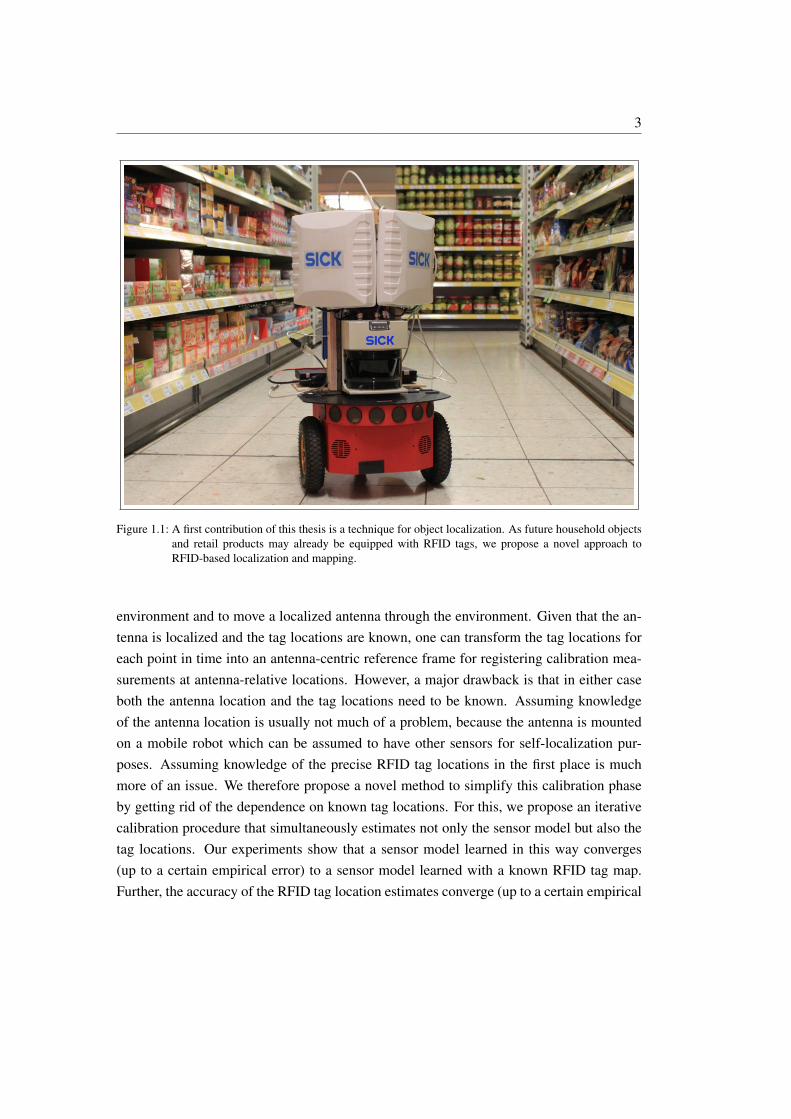
Figure 1.1: A first contribution of this thesis is a technique for object localization. As future household objectsand retail products may already be equipped with RFID tags, we propose a novel approach toRFID-based localization and mapping.
environment and to move a localized antenna through the environment. Given that the an-tenna is localized and the tag locations are known, one can transform the tag locations foreach point in time into an antenna-centric reference frame for registering calibration mea-surements at antenna-relative locations. However, a major drawback is that in either caseboth the antenna location and the tag locations need to be known. Assuming knowledgeof the antenna location is usually not much of a problem, because the antenna is mountedon a mobile robot which can be assumed to have other sensors for self-localization pur-poses. Assuming knowledge of the precise RFID tag locations in the first place is muchmore of an issue. We therefore propose a novel method to simplify this calibration phaseby getting rid of the dependence on known tag locations. For this, we propose an iterativecalibration procedure that simultaneously estimates not only the sensor model but also thetag locations. Our experiments show that a sensor model learned in this way converges(up to a certain empirical error) to a sensor model learned with a known RFID tag map.Further, the accuracy of the RFID tag location estimates converge (up to a certain empirical

4 Chapter 1 Introduction
error) to the true tag locations. We like to point out that this iterative procedure is onlynecessary if the sensor model should be learned without the reliance on a known RFIDtag map. We quantitatively evaluate our approach and variants thereof in an office and asupermarket environment, also by comparing it to previously published sensor models. Forthis, we implemented and adapted a WiFi-based localization method, which constructs a2D signal strength map by using Gaussian process regression. We additionally extend thisapproach by mapping the signal strength in pose space rather than in 2D. This is particularrelevant for RFID-based localization, as the received signal strength can be quite sensitiveto rotational changes of the antenna pose.
Given that the robot can localize objects, we move on to the question of how prior knowl-edge about usual object arrangements can be utilized by the robot to more efficiently carryout its tasks, particularly, when searching for objects in an unknown environment. As a mo-tivation, consider the situation where you want to find a product in a supermarket where youhave never been to before. Certainly, you will not just wander around randomly throughthe market nor will you systematically visit each so far unvisited aisle in the market untilyou find the product. Your search will rather be guided by the current observations andthe expectations you have about how objects in supermarkets are usually arranged. Youwill have gained this knowledge by having seen quite a few markets throughout your lifeand noting certain strong spatial dependencies between certain groups of products. Thus,the main challenge that we need to address here is to, first, formalize this knowledge ina way such that it can be learned based on data of real supermarkets and, second, to de-vise a search strategy that leverages this knowledge in an appropriate way to speed up thesearch process. For this, we present two alternative search techniques. Our first approachis a reactive search technique that decides where to search next based on the objects in therobot’s direct vicinity. The robot utilizes search heuristics in form of decision trees whichclassify the aisles at junctions into promising and non-promising directions and then con-tinues to search in one of the promising directions. The decision trees are learned fromdata generated from optimal search paths in a training set of supermarkets. In contrast tothe first approach, our second search technique is a more global, inference-based approachthat takes into account all objects seen so far as well as the thus far discovered structureof the environment. Based on this, it first computes a distribution over the possible loca-tions of the sought product. Then it selects a goal location by trading off the probabilityof finding the product at a certain location against the required distance to reach this loca-tion. It then continues its search by following the shortest path towards the selected goallocation. Whenever new information becomes available, i.e., newly observed objects or
5
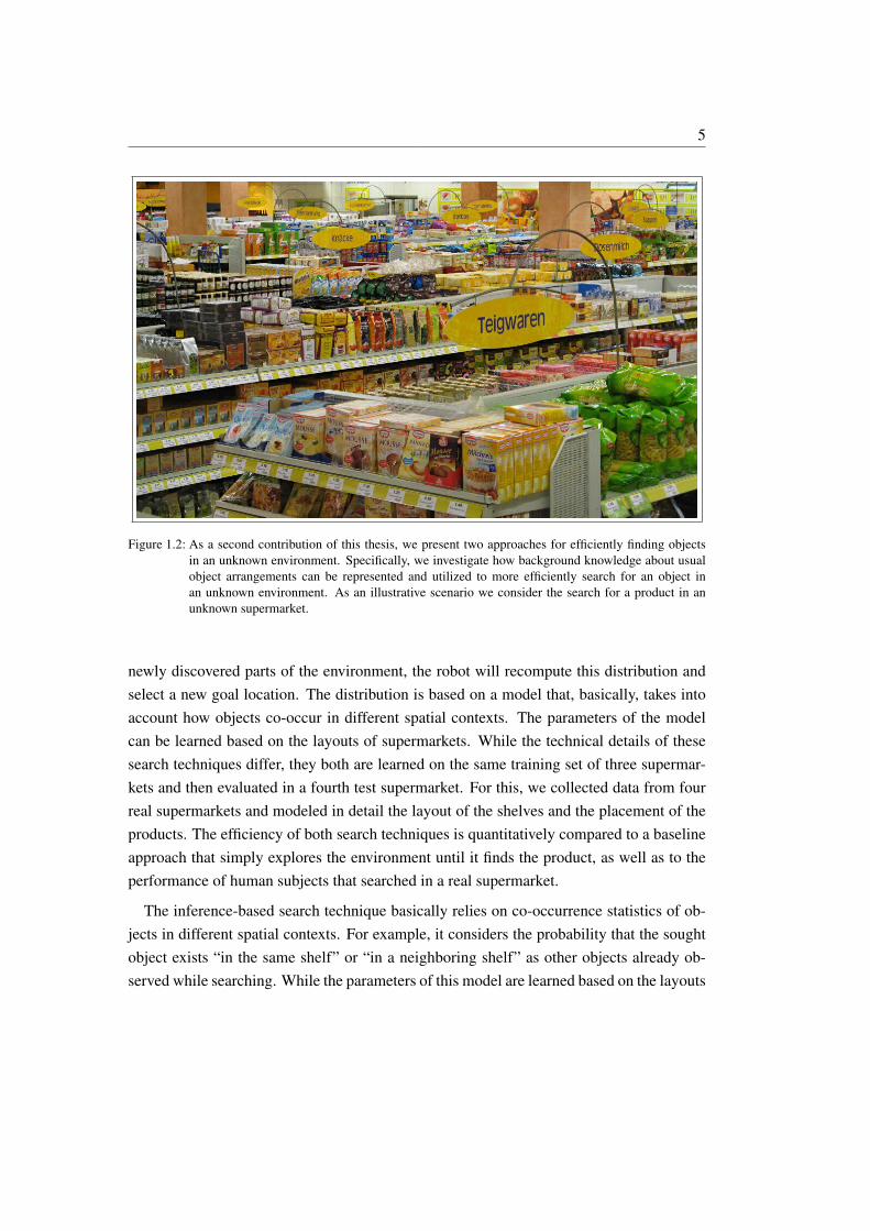
Figure 1.2: As a second contribution of this thesis, we present two approaches for efficiently finding objectsin an unknown environment. Specifically, we investigate how background knowledge about usualobject arrangements can be represented and utilized to more efficiently search for an object inan unknown environment. As an illustrative scenario we consider the search for a product in anunknown supermarket.
newly discovered parts of the environment, the robot will recompute this distribution andselect a new goal location. The distribution is based on a model that, basically, takes intoaccount how objects co-occur in different spatial contexts. The parameters of the modelcan be learned based on the layouts of supermarkets. While the technical details of thesesearch techniques differ, they both are learned on the same training set of three supermar-kets and then evaluated in a fourth test supermarket. For this, we collected data from fourreal supermarkets and modeled in detail the layout of the shelves and the placement of theproducts. The efficiency of both search techniques is quantitatively compared to a baselineapproach that simply explores the environment until it finds the product, as well as to theperformance of human subjects that searched in a real supermarket.
The inference-based search technique basically relies on co-occurrence statistics of ob-jects in different spatial contexts. For example, it considers the probability that the soughtobject exists “in the same shelf” or “in a neighboring shelf” as other objects already ob-served while searching. While the parameters of this model are learned based on the layouts
6 Chapter 1 Introduction
of supermarkets in a training set, the spatial relations utilized by this model are fixed andmanually defined. Thus, in our final contribution of this thesis, we move on to a moreambitious learning scenario in which we wish to simultaneously learn both the spatial con-text and the co-occurrence of objects within the learned spatial contexts. That is, we wishto learn spatially coherent object constellations in complex multi-object scenes in an un-supervised way. As an application scenario we considered tabletop scenes and the objectconstellations are the covers consisting of, for example, a plate, a knife, and a mug. Theidentification of the relevant object constellations can be seen as parsing a scene or inferringthe latent structure of a scene. However, for any given scene there exist multiple possiblescene structures. For example, in the scene depicted in Fig. 1.3 we could argue that itsimply contains twelve randomly placed objects. Alternatively, one might say that it con-tains just a single object constellation consisting of twelve objects. However, based on ourprior knowledge of tabletop scenes, we would be tempted to say that it is much more likelythat this scene contains three recurrent object constellations each consisting of four objects,namely a plate, a fork, a knife, and a mug. We will make this notion of “a more likely scenestructure” precise, by defining a prior distribution over scene structures. This prior can thenbe used to evaluate the probability of each of the three above-mentioned alternative scenestructures. Further, this prior can be updated by conditioning it on previously parsed sceneswhich results in a posterior predictive distribution over scenes. Thus, if the robot has neverobserved any such scene, it may consider the three alternative scene interpretations as moreor less equally likely. However, if the robot has already parsed several scenes in whichsimilar object constellations with four objects appear, then it might agree with our intuitionthat the scene most likely contains three object constellations with four objects each.
To be more specific, we define a novel hierarchical nonparametric Bayesian model formulti-object scenes. A basic building block of our model are so-called meta-objects whichrepresent a distribution over object constellations. The actual object constellations on thetable are assumed to have been sampled from such meta-objects. More specifically, meta-objects can be seen as probabilistic part-based models and they thus have an internal struc-ture. Each part of a meta-object consists of (a) a spatial distribution that constrains therelative location of an object with respect to a meta-object reference frame, (b) a type dis-tribution that constrains which objects should be placed there (e.g., a mug or plate), and(c) an activation probability that specifies the probability if an object should be placed atthis location at all. A meta-object for the constellations shown in Fig. 1.3 would consistof four parts, e.g., a central part with a high probability for plates, a left part with a highprobability for forks, etc. For sampling a constellation from this model, we first sample the

7
Figure 1.3: As a third contribution of this thesis, we investigate how a robot can learn spatially coherent objectconstellations in an unsupervised way by inferring the latent structure of everyday scenes. Weconsider tabletop scenes, in which the relevant object constellations correspond to the individualcovers consisting of, for example, a plate, a knife, a fork, and a mug.
activation for each part. For each activated part, we then sample the relative location andthe object type to be placed at this relative location, e.g., a mug or a plate. Hence, each partgenerates at most one object of a sampled object constellation. This object constellationis then transformed into the scene by sampling from a prior over transformations. We as-sume that a scene can contain multiple object constellations, such as the scene in the pictureshown above, which contains three object constellations that have been transformed to threedifferent places on the table. Further, we assume that there exist different types of objectconstellations, which might have different parametrizations of their part distributions. Forexample, one specific meta-object type might likely generate a constellation with a cerealbowl and a spoon, while another type would more likely generate object constellations likethe ones mentioned above. Thus, parsing a scene corresponds to inverting this generativeprocess by inferring the number of object constellations in a scene, their types, and theirtransformations or reference frames. Further, the objects on a table need to be associated toa certain meta-object instance as well as to a certain part of this meta-object instance. For
8 Chapter 1 Introduction
example, the plate should be associated to the central part of its meta-object.Please note, that we did not yet specify the number of meta-object types, the number of
parts per meta-object, or the number of object constellations on the table. Actually, it wouldbe desirable to avoid having to specify these numbers in advance and we would rather like toplace a prior over these numbers and infer them from data. This is achieved by formulatingour model as a nonparametric Bayesian model based on the Dirichlet process and the beta-Bernoulli process. By doing so, we do not even have to specify an upper bound for thesenumbers. Rather, we thereby assume that there exist infinitely many different meta-objecttypes, each having infinitely many parts. In effect, the number of meta-object types andthe number of meta-object parts are now subject to inference as well and we can set certainhyper-parameters which express our prior belief with respect to these numbers. This allowsfor a probabilistic treatment of the effective model complexity which thereby can adapt tothe data complexity. This also has practical benefits in the context of lifelong learning forservice robots. As the number of object constellations is not fixed in our model, the robotis able to recognize and integrate previously unseen object constellations into its model inan open-ended fashion and within a single coherent probabilistic framework.
1.1 Contributions
The work presented in this thesis contributes to mainly three areas in the context of mobilerobotics: (a) RFID-based localization and mapping, (b) object search in unknown environ-ments, and (c) scene analysis. In particular, we like to highlight the following contributions.
1.1.1 RFID-based Localization and Mapping
• A novel probabilistic sensor model for RFID-based localization and mapping. Incontrast to previously published models, our model considers both signal strengthand tag detection events.
• A novel unsupervised procedure for simultaneously learning both the sensor modeland the tag locations in an iterative manner. This generalizes a supervised non-iterative method for learning the sensor model which is only applicable when thetag locations are known beforehand.
• For evaluation purposes, an adaption of a previously published sensor-centric RFIDsensor model.
1.1 Contributions 9
• For evaluation purposes, an adaption of a previously published WiFi-based sensormodel based on Gaussian process regression. The model is further extended to mapthe signal strength in pose space rather than in 2D.
• An extensive evaluation of our method in an office and a supermarket environment.
1.1.2 Object Search in Unknown Environments
• A novel reactive search technique that utilizes search heuristics in form of decisiontrees which classify the aisles at junctions into promising and non-promising direc-tions. The robot then continues to search in one of the promising directions.
• A technique to learn these decision trees based on data generated from optimal searchpaths in training environments.
• An inference-based search technique that maintains a distribution over the possiblelocation of the object. This distribution takes into account all objects seen so far andthe thus far discovered structure of the environment.
• A technique to learn the parameters of this model based on the layout of trainingenvironments.
• An extensive evaluation of both techniques, including a comparison to a baselinetechnique, that explores the supermarket until it finds the product, and to the perfor-mance of human subjects that participated in a field study conducted in a real market.
1.1.3 Scene Analysis
• A novel probabilistic approach to reason about the latent structure of multi-objectscenes in terms of object constellations. For this, we propose a novel hierarchi-cal nonparametric Bayesian model based on nested and hierarchical variants of theDirichlet process (or Chinese restaurant process) and the beta-Bernoulli process (orIndian buffet process).
• A Markov chain Monte Carlo procedure to sample from the posterior distributionover the latent scene structures when conditioned on the observed objects of thescenes. This includes efficient MCMC moves that propose to change the correspon-dence variables of several observed objects at a time. Further, we introduce a novel

10 Chapter 1 Introduction
top-down bottom-up proposal for the MCMC sampler that takes advantage of boththe observed data and the currently instantiated representations in the model.
• An evaluation of the proposed MCMC technique for obtaining samples from theposterior distribution of our model when conditioned on tabletop scenes from bothsynthetic and real-world data sets.
1.2 Publications
Parts of the work presented in this thesis have been previously published in the followingjournal and conference publications. All publications were peer-reviewed except wherenoted. For each publication, we point out the related chapter in this thesis.
Journal
• Dominik Joho, Martin Senk, and Wolfram Burgard. Learning search heuristicsfor finding objects in structured environments. Robotics and Autonomous Systems(RAS), 59(5):319–328, May 2011.Related: Chap. 4
Conference
• Dominik Joho, Gian Diego Tipaldi, Nikolas Engelhard, Cyrill Stachniss, and Wol-fram Burgard. Nonparametric Bayesian models for unsupervised scene analysis andreconstruction. In Proc. of Robotics: Science and Systems (RSS), Sydney, Australia,2012.Related: Chap. 5
• Dominik Joho and Wolfram Burgard. Searching for objects: Combining multiplecues to object locations using a maximum entropy model. In Proc. of the IEEE Int.Conf. on Robotics and Automation (ICRA), pages 723–728, Anchorage, AK, USA,May 2010.Related: Chap. 4
• Dominik Joho, Christian Plagemann, and Wolfram Burgard. Modeling RFID signalstrength and tag detection for localization and mapping. In Proc. of the IEEE Int.Conf. on Robotics and Automation (ICRA), pages 3160–3165, Kobe, Japan, May
1.3 Collaborations 11
2009.Related: Chap. 3
• Dominik Joho, Martin Senk, and Wolfram Burgard. Learning wayfinding heuristicsbased on local information of object maps. In Proc. of the Europ. Conf. on MobileRobots (ECMR), pages 117–122, Mlini/Dubrovnik, Croatia, September 2009.Related: Chap. 4
Workshop
• Dominik Joho, Gian Diego Tipaldi, Nikolas Engelhard, Cyrill Stachniss, and Wol-fram Burgard. Unsupervised scene analysis and reconstruction using nonparametricBayesian models. In Proc. of the Workshop on Robots in Clutter at Robotics: Sci-ence and Systems (RSS), Sydney, Australia, 2012.Related: Chap. 5
Extended Abstract (not peer-reviewed)
• Dominik Joho, Gian Diego Tipaldi, Nikolas Engelhard, Cyrill Stachniss, and Wol-fram Burgard. Unsupervised scene analysis using semiparametric Bayesian models.In Extended Abstracts of Spatial Cognition (SC), Kloster Seeon, Germany, 2012.Related: Chap. 5
1.3 Collaborations
The search strategy based on decision trees is one of two search strategies presented inChap. 4 and was originally addressed in the co-supervised Bachelor’s thesis of Martin Senk[63]. The same chapter presents results of a field study conducted with human participantsin a real supermarket. This field study was carried out by Christopher Kalff and colleaguesof the Center for Cognitive Science at the University of Freiburg. To track the participantsin the supermarket, Christopher Kalff and colleagues used our proposed RFID-based local-ization system. The resulting trajectories and performance metrics were then used by usfor a comparison with our proposed search technique. In Chap. 5, the segmentation andclassification of the pointclouds of the tabletop scenes has been implemented by NikolasEngelhard.

12 Chapter 1 Introduction
1.4 Notation
In Tab. 1.1 we illustrate notational conventions used throughout this thesis. Please note thatthere is an ambiguity whether a boldface x denotes (a) a vector, (b) the outcome x1, . . . , xn
of a collection of scalar random variables, or (c) the outcome x1, . . . ,xn of a collection ofvector-valued random variables. It should be clear from the context which case applies andwe will therefore not further resolve this issue.
Table 1.1: Some notational conventions used in this thesis.
Symbol Meaning
Algebra and Geometry
x scalarx vectorxT transposed vectorX matrixa ∝ b a is proportional to b
Probability Theory and Monte Carlo Methods
X random variableX multiple random variablesx possible outcome of a random variable, e.g. X = xx multiple outcomes of the corresponding random variables, e.g. X = xx1:t sequence of outcomes, x1:t = x1, . . . , xtp(x) probability mass function or probability density functionp(z | x) conditional probability of z given xx ∼ Dist x is distributed according to Distδx(·) Dirac delta function centered at xEp(X) expectation (expected value) of random variable X wrt. the distribution pH(p) entropy of the distribution p
Probability Distributions and Stochastic Processes
BP beta processBern Bernoulli distributionBeP Bernoulli processCRP Chinese restaurant processDir Dirichlet distributionDP Dirichlet processGP Gaussian processIBP Indian buffet processMult multinomial distributionN normal distribution (Gaussian distribution)NW normal-Wishart distributionPois Poisson distribution

CHAPTER 2
Basics
We review some of the theoretical foundations underlying the techniquespresented in later chapters. We aim at giving a concise yet readable in-troduction to the various topics and we provide pointers to the literaturefor the interested reader who desires a more in-depth treatment of thesetopics.
We start by reviewing the basics of probability theory, which is the foundation for manyof the topics to follow. We then proceed with an introduction to Monte Carlo methods,including particle filtering and Markov chain Monte Carlo (MCMC) methods. Particlefiltering is a frequently used technique for mobile robot localization. It will be utilized inChap. 3 for estimating the trajectory of a sensor platform moving through an RFID-enabledenvironment. MCMC techniques will be of importance in Chap. 5 for performing posteriorinference in a generative probabilistic model of tabletop scenes. We then describe decisiontrees, that will be used as a way to learn and represent search heuristics in Chap. 4. Next,we discuss maximum entropy models, which will be used in the same chapter for modelinga distribution over the possible locations of an object the robot is searching for. Finally, wehave a section on Bayesian nonparametrics, which covers three commonly used stochasticprocesses. The first two processes, the Dirichlet process and the beta-Bernoulli process,are the corner stones for our proposed hierarchical model of tabletop scenes that we willdescribe in Chap. 5. The third stochastic process, the Gaussian process, is used in Chap. 3 torepresent signal strength maps as an alternative RFID localization method that we evaluatealongside our proposed antenna-centric approach.
14 Chapter 2 Basics
2.1 Basics of Probability Theory
Mobile robots are autonomous systems that act in a flexible and adaptive way by observingthe world and by making their actions dependent on the current state of the world. For this,the robot needs to acquire information about the current state of the world, including itsown state, and it needs to reason about how the state might evolve over time as well as howits own actions might influence this state. Obviously, all three stages – sensing, planning,acting – involve substantial uncertainties. A robot never directly observes the true state ofthe world. Rather, it has to infer this state from sensor data, which might be inherentlyambiguous with regard to this state and, additionally, it might be subject to measurementnoise. Planning needs to deal with uncertainties, as the robot can never actually predict thefuture states of the world with absolute certainty. Likewise, the outcome of its own actionsare uncertain, too, be it because a wheel slips on the ground or its gripper misses the bottleon the table. A formal system to deal with uncertainty in a consistent way is probabilitytheory. Not surprisingly, there exists a wide range of techniques in mobile robotics thathave their theoretical foundation in probability theory [74] and many of the techniquesbeing used in this thesis are also based on probability theory. In the following, we willtherefore shortly review the basics of probability theory [59, 74].
Like propositional logic, probability theory deals with statements. However, in contrastto propositional logic, these statements are not considered to be either true or false but tobe more or less likely. Hence, a statement is assigned a continuous value, a probability, inthe interval [0, 1]. Further, probability theory formalizes a consistent way for calculating,or inferring, probabilities for statements based on the probabilities of other statements.Equivalently, one might say probability theory deals with random events and the statementsare about the possible outcome of events. For example, consider the cast of a die. Then Xcould be the random event that denotes the number of dots the die will show after it hasbeen cast. Then X = 2 is a statement about the outcome of this event, namely that the diewill show 2 dots. If we think it is a fair die, we might assign the probability p(X = x) = 1
6
for all possible outcomes x ∈ 1, . . . , 6. In this example, X is a discrete random variablewith sample space X = 1, . . . , 6 and with a uniform discrete distribution p.
More formally, a random variable X is defined over a sample space X that defines allpossible outcomes and p is a probability distribution over the sample space X . For discreterandom variables, p is a probability mass function (PMF) and we denote by p(X = x) theprobability that the random variable will assume the value x. Often, we will simply writep(x) for p(X = x). For continuous variables, p is a probability density function (PDF) and

2.1 Basics of Probability Theory 15
we denote by p(y) the value of the density function at y and by p(Y ∈ A) we denote theprobability of the event that the random variable Y assumes a value in the subset A ⊆ Ywith Y being the corresponding sample space. Probability distributions need to satisfycertain consistency properties. First, a probability is a real in the interval [0, 1], hence
p(X = x) ∈ [0, 1] for all x ∈ X and p is a PMF (2.1)
p(Y ∈ A) ∈ [0, 1] for all A ⊆ Y and p is a PDF (2.2)
Next, the probabilities for discrete random variables sum to one and the density functionfor continuous variables integrates to one.∑
x∈Xp(X = x) = 1 p is a PMF (2.3)∫
y∈Yp(y) dy = 1 p is a PDF (2.4)
Further, probabilities are additive in the sense that for mutually exclusive events A =
a1, . . . , an with ai ⊆ X and ai ∩ aj = ∅ for i 6= j we have for a PMF p
p(X = A) = p(X = a1 or . . . or X = an) (2.5)
= p(X = a1) + · · ·+ p(X = an) (2.6)
and likewise for a PDF p with the corresponding adjustments in notation, e.g. p(Y ∈ A)
instead of p(X = A) and the a1, . . . , an then form a partition of the subset A ⊆ Y .For ease of exposition, we assume for the rest of this section that all variables are discrete.Some further properties that follow from the above-said are the certain event
p(X ) = 1 (2.7)
the impossible event
p(∅) = 0 (2.8)
and the complementary event
p(A) = 1− p(X\A). (2.9)
16 Chapter 2 Basics
In any practical setting, we will have to deal with multiple random variables, e.g. X andY , and their joint distribution p(x, y) which corresponds to the event that X = x holdsand that Y = y holds. A joint distribution can be factorized into conditional distributionsaccording to the chain rule
p(x, y) = p(x | y)p(y) = p(y | x)p(x). (2.10)
Here, the conditional distribution p(x | y) is the distribution for the random variable Xgiven that we know (with certainty) that Y = y is the case. If the knowledge of the valueof Y tells us nothing about the possible values of X , then this would keep the distributionfor X unchanged such that p(x | y) = p(x) and we say these variables are independent.Hence in this case we would have
p(x, y) = p(x)p(y) X and Y are independent. (2.11)
An important variant thereof is conditional independence, in which two variables X andY are dependent, but become independent when given knowledge of the value of a thirdrandom variable Z. In this case, we say X and Y are conditionally independent given Zand we have
p(x, y, z) = p(x, y | z)p(z) (2.12)
= p(x | z)p(y | z)p(z) X and Y are cond. indep. given Z. (2.13)
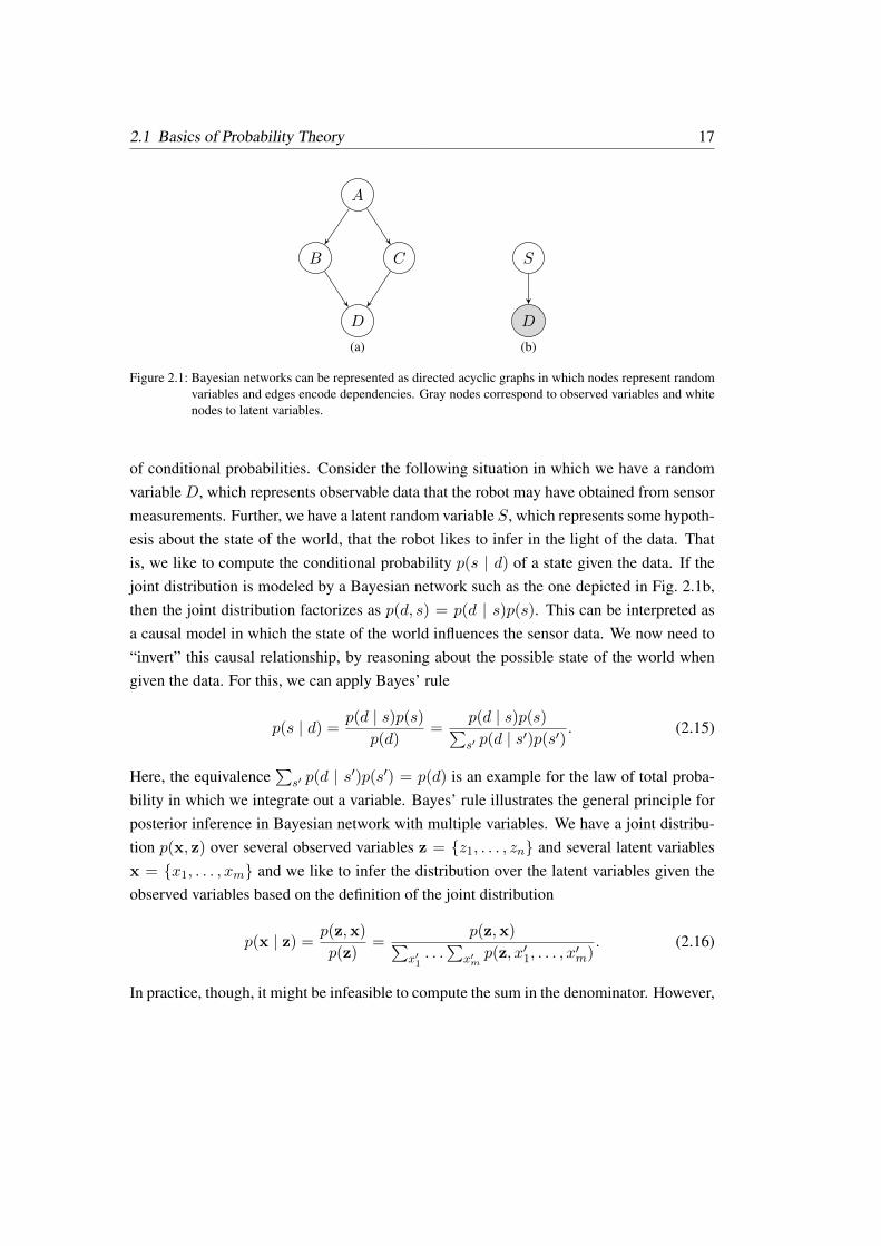
In practice, we will often deal with distributions with more than two variables. One wayof modeling complex joint distributions over multiple variables are Bayesian networks inwhich we assume certain conditional independencies between these variables and factor-ize the joint distribution into conditional distributions. These conditional distributions canthen be modeled by standard distributions such as the Gaussian distribution or the Poissondistribution. The joint distribution can be represented as a directed acyclic graph like theone depicted in Fig. 2.1a. The joint factorizes into conditional distributions for each of thenodes, where the random variable of a node is conditioned on the random variables of itspredecessor nodes or parent nodes. Hence, for the example in Fig. 2.1a we have
p(a, b, c, d) = p(d | b, c)p(b | a)p(c | a)p(a). (2.14)
A further important concept is Bayes’ rule, which directly follows from the definition
2.1 Basics of Probability Theory 17
A
B C
D
(a)
S
D
(b)
Figure 2.1: Bayesian networks can be represented as directed acyclic graphs in which nodes represent randomvariables and edges encode dependencies. Gray nodes correspond to observed variables and whitenodes to latent variables.
of conditional probabilities. Consider the following situation in which we have a randomvariable D, which represents observable data that the robot may have obtained from sensormeasurements. Further, we have a latent random variable S, which represents some hypoth-esis about the state of the world, that the robot likes to infer in the light of the data. Thatis, we like to compute the conditional probability p(s | d) of a state given the data. If thejoint distribution is modeled by a Bayesian network such as the one depicted in Fig. 2.1b,then the joint distribution factorizes as p(d, s) = p(d | s)p(s). This can be interpreted asa causal model in which the state of the world influences the sensor data. We now need to“invert” this causal relationship, by reasoning about the possible state of the world whengiven the data. For this, we can apply Bayes’ rule
p(s | d) =p(d | s)p(s)
p(d)=
p(d | s)p(s)∑s′ p(d | s′)p(s′)
. (2.15)
Here, the equivalence∑
s′ p(d | s′)p(s′) = p(d) is an example for the law of total proba-bility in which we integrate out a variable. Bayes’ rule illustrates the general principle forposterior inference in Bayesian network with multiple variables. We have a joint distribu-tion p(x, z) over several observed variables z = z1, . . . , zn and several latent variablesx = x1, . . . , xm and we like to infer the distribution over the latent variables given theobserved variables based on the definition of the joint distribution
p(x | z) =p(z,x)
p(z)=
p(z,x)∑x′1. . .∑
x′mp(z, x′1, . . . , x
′m). (2.16)
In practice, though, it might be infeasible to compute the sum in the denominator. However,
18 Chapter 2 Basics
any quantity that depends on the distribution p(x | z) can be approximated by drawingsamples from this distribution and basing the calculations on the obtained samples. This isthe basic idea of Monte Carlo methods, which we will describe in the following.
2.2 Monte Carlo Methods
Monte Carlo methods [2, 46, 74] can be used to approximate intractable integrals or sums,such as expectations with respect to a probability distribution p(x). In this case, the mainidea is to obtain a set of samples x(1), . . . , x(N) from a distribution p(x) over the samplespace X and then to approximate the expectation
Ep(f(x)) =
∫x∈X
f(x)p(x) dx (2.17)
by the Monte Carlo approximation based on the samples
EN (f(x)) =1
N
N∑i=1
f(x(i)). (2.18)
The main problem here is to obtain samples from the distribution p(x). If the distributionp(x) is of some standard form, such as a Gaussian, then there might exist dedicated algo-rithms for directly drawing samples. However, for the general case of arbitrarily shapeddistributions or density functions, we need more generally applicable methods for drawingsamples. In the following, we will describe two widely used techniques for this: importancesampling and Markov chain Monte Carlo. Further, we describe a sequential Monte Carlomethod for sampling from a dynamic Bayesian network that forms the basis for mobilerobot localization.
2.2.1 Importance Sampling
In importance sampling [14, 74], we side-step the impracticality of directly sampling fromp(x) by introducing an auxiliary proposal distribution q(x) from which we can easily sam-ple. The samples from the proposal q(x) are then carefully adjusted such that they appearto be sampled from the target distribution p(x) that we are actually interested in. For this,the proposal distribution q(x) must have the same support X as the target distribution. Thefollowing derivation is based on [14]. Remember that our initial attempt was to computethe integral of Eq. (2.17), which we could rewrite by introducing the proposal distribution
2.2 Monte Carlo Methods 19
q(x) as follows
Ep(f(x)) =
∫f(x)p(x) dx (2.19)
=
∫f(x)
p(x)
q(x)q(x) dx. (2.20)
Let us define the so-called importance weight as w(x) ≡ p(x)q(x) and remember that
∫w(x)q(x) dx =
∫p(x)
q(x)q(x) dx = 1. (2.21)
Then we have
Ep(f(x)) =
∫f(x)
p(x)
q(x)q(x) dx (2.22)
=
∫f(x)w(x)q(x) dx (2.23)
=
∫f(x)w(x)q(x) dx∫w(x)q(x) dx
(2.24)
Both integrals appearing in Eq. (2.24) can be approximated by a Monte Carlo estimate withrespect to N samples x(1), . . . , x(N) drawn from q(x), which leads to
EN (f(x)) =1N
∑i f(x(i))w(x(i))
1N
∑iw(x(i))
(2.25)
=∑i
f(x(i))w(x(i))∑i′ w(x(i′))
(2.26)
=∑i
f(x(i))w(x(i)), (2.27)
where
w(x(i)) ≡ w(x(i))∑i′ w(x(i′))
(2.28)
is the normalized importance weight of sample x(i). Please note, that this method is also
20 Chapter 2 Basics
applicable if the target distribution p(x) is known only up to a normalizing constant, be-cause this constant would cancel in Eq. (2.24) where it appears in each occurrence of theimportance weight w(x).
To summarize, we draw samples from q(x) and compute the normalized weights for eachsample based on the proposal density and the target density. Intuitively, we may say thatthe target distribution is now (approximately) represented by the set of weighted samples.Especially, the samples can be used to compute Monte Carlo estimates of expectations withrespect to the original target distribution.
However, there is the drawback that importance sampling depends on a well-designedproposal distribution that should closely match the target distribution over the whole samplespace. Otherwise, we would “loose” many samples in low-probability regions of the targetdistributions. For arbitrarily shaped target distributions it may become difficult to findappropriate proposal distributions from which we can easily sample. Further, this willbecome even more problematic for high-dimensional target distributions. In such situations,we can apply Markov chain Monte Carlo methods, that we describe in the next section.
2.2.2 Markov Chain Monte Carlo
The main difficulty of importance sampling was to find a proposal distributions that globallymatches the target distribution as close as possible. Further, the samples have been drawnindependently of each other. If one sample happens to be in a high-probability region ofthe target distribution, then this will have no influence on subsequent samples. Roughlyspeaking, we would like to utilize this information and try to “explore” or search the spacein this region. This idea is taken up by Markov chain Monte Carlo (MCMC) methods,in which we can utilize proposal distributions q(x | x(i)) that may depend on the latestsample x(i). For example, we could sample from a proposal distribution that puts most ofits probability mass around a local neighborhood of x(i). We thereby get a sequence ofsamples that move through the state space in small steps. However, if these samples shouldrepresent draws from the target distribution, we must take care to also make this sequencedependent on the target distribution in an appropriate way.
One commonly used MCMC method is the Metropolis-Hastings algorithm [2]. We aregiven a target distribution p(x) known up to a normalization constant, a proposal distribu-tion q(x′ | x), and an arbitrary initial sample x(0). We then iterate the following. Based onthe current sample x(i), we propose a new sample x? drawn from the proposal q(x? | x(i)).
2.2 Monte Carlo Methods 21
We then compute the acceptance ratio
R =p(x?)q(x(i) | x?)p(x(i))q(x? | x(i))
, (2.29)
and set the new sample x(i+1) to
x(i+1) =
x? with probability min(1, R)
x(i) with probability 1−min(1, R). (2.30)
Thus, the proposed sample x? is either accepted or rejected with a probability dependingon the acceptance ratio R. If the sample is accepted, the Markov chain “moves” to thisproposed location, otherwise, it “stays” at the current location. The obtained sample is thenadded to the set of samples that represent draws from the target distribution. Thus, if thechain stays at the current location, the obtained sample is once again added to the set ofsamples.
Another MCMC method is Gibbs sampling, which can be derived as a special case ofthe Metropolis-Hastings algorithm. The following derivation is based on [2]. In Gibbssampling, we have a multidimensional state space x = (x1, . . . , xn) and we propose anew sample by changing only a single variable xj while the other variables, denoted asx[−j], remain unchanged. Thus, based on the i-th sample x(i) we would propose a sample
x? = (x(i)1 , . . . , x
(i)j−1, x
?j , x
(i)j+1, . . . , x
(i)n ). The proposal distribution draws x?j from the full
conditional distribution p(x?j | x(i)[−j]) of the target distribution, and hence
qj(x? | x(i)) =
p(x?j | x(i)[−j]) if x?[−j] = x
(i)[−j]
0 otherwise. (2.31)
The acceptance ratio for a sample proposed in this way is
R =p(x?)
p(x(i))
qj(x(i) | x?)
qj(x? | x(i))(2.32)
=p(x?)
p(x(i))
p(x(i)j | x?[−j])
p(x?j | x(i)[−j])
(2.33)
=p(x?j | x
(i)[−j])p(x
(i)[−j])
p(x(i)j | x?[−j])p(x
?[−j])
p(x(i)j | x?[−j])
p(x?j | x(i)[−j])
(2.34)

22 Chapter 2 Basics
=p(x
(i)[−j])
p(x?[−j])(2.35)
= 1. because x(i)[−j] = x?[−j] (2.36)
Thus, the proposed sample is always accepted. During Gibbs sampling we would apply thisstep for each dimension or variable of the state space, either in a fixed or random order. Themain drawbacks of a Gibbs sampler are twofold. First, we must be able to draw samplesfrom the full conditional distribution of the target distribution. If it is impossible to directlysample from this conditional, then this could be side-stepped by using Metropolis-Hastingssteps to sample from the conditional. This is known as “Metropolis within Gibbs”. Second,because we are only changing a single variable at a time the sampler might easily getstuck in local minima if there exist strong dependencies between several variables. In thiscase, it is beneficial to extend the principle of Gibbs sampling to the case where we jointlypropose new values for these strongly correlated variables. This is known as blocked Gibbssampling. However, as more variables are clumped together in one block, it might becomeincreasingly difficult to devise a sampling strategy to jointly draw new values for thesevariables from the implied conditional distribution of the target distribution.
In practical applications of MCMC methods, one usually ignores the first couple of sam-ples during a “burn-in” period. This is, because the initial sample x(0) usually lies in aregion of low probability and the Markov chain first has to reach regions of high probabil-ity and, therefore, the first samples are not representative for the target distribution. Further,one could take into account only every n-th sample of the chain to minimize the correlationbetween the samples. In contrast to importance sampling, MCMC methods can take ad-vantage of having found regions of high probability by exploring these regions with localmoves from the proposal. However, if the target distribution is multimodal and the modesare far apart, it may easily happen that the chain only explores a single mode. One could tryto avoid this by starting several independent chains from different initial locations. Further,one could propose more global moves from time to time in the hope of reaching an areaclose to another mode. Hence, it is apparent that also for MCMC methods it can be difficultto come up with well-designed proposal distributions.
2.2.3 Monte Carlo Localization for Mobile Robots
Monte Carlo localization [21, 74] is an approach for tracking the pose of a robot by formal-izing the tracking problem as in inference problem in a dynamic Bayesian network such as

2.2 Monte Carlo Methods 23
x0
u1
x1
u2
x2
u3
x3 . . .
z1 z2 z3
m
Figure 2.2: The Bayesian network used for mobile robot localization. Gray nodes denote observed variables.
the one depicted in Fig. 2.2. The robot’s pose is modeled as a latent variable xt that evolvesover time in discrete steps. The motion model p(xt | xt−1, ut) describes how the pose at acertain time t depends on the previous pose xt−1 and the latest motion command or controlut of the robot. Further, this distribution could depend on the map m to model impossibletransitions through walls, though for simplicity we omit this here. At each time step, therobot takes a sensor measurement zt and the senor model p(zt | xt,m) describes how ameasurement depends on the current pose of the robot and a given map m of the environ-ment. For localization purposes, we are interested in the belief bel(xt) as a distributionover the current location of the robot. This corresponds to the posterior distribution
bel(xt) = p(xt | z1:t, u1:t,m) (2.37)
over the current pose of the robot conditioned on the map and all past measurements andcontrols. Further, all past states have been integrated out. To compute the belief for the nexttime step, we first compute the predictive distribution bel(xt+1) which is the distributionthat takes into account the next control ut+1 but does not yet include the information aboutthe next measurement
bel(xt+1) = p(xt+1 | z1:t, u1:t+1,m) (2.38)
=
∫xt
p(xt+1 | xt, ut+1) bel(xt) dxt. (2.39)
Finally, the predicted belief is adjusted by incorporating the information about the new
24 Chapter 2 Basics
measurement zt and hence
bel(xt+1) ∝ p(zt+1 | xt+1)bel(xt+1). (2.40)
In Monte Carlo localization the state distribution is represented nonparametrically by aset of weighted samples called particles and the resulting method is also called a particle fil-ter. As argued in [74], the particle filter can actually be thought of estimating a distributionbel(x1:t) over the full trajectory x1:t = x1, . . . , xt instead of just the filtering distributionbel(xt) over the last pose xt. Thus, the set of weighted particles x(i)
1:t, w(i)t Ni=1 represents
an estimate of bel(x1:t). However, if we simply ignore the past states x(i)1:t−1 of each parti-
cle, then x(i)t , w
(i)t Ni=1 also defines an estimate of the desired filtering distribution bel(xt)
over the current state.
The particle filter then starts with an initial distribution over the first time step and thenadjusts the particle set to represent a distribution over successively longer histories. Indetail, this works as follows:
• Initialization: Initialize the particle set once by drawing each particle from the priorx
(i)0 ∼ p(x0) and set the weights uniformly to w(i)
0 = 1N .
• Prediction: For each particle x(i)1:t, sample a new state for the next time step by sam-
pling from the motion model x(i)t+1 ∼ p(xt+1 | x(i)
t , ut) and append this state to thehistory of the particle.
• Update: Compute the new importance weight of each particle w(i)t+1 = p(zt+1 |
x(i)t+1,m) and then normalize the weights.
• Resampling: Resample N particles from the particle set according to their currentweights. Then set w(i)
t+1 = 1N for each particle.
The weighing of the particles in the update step accounts for the fact that the particleshave been sampled from the predictive distribution
bel(x1:t+1) = p(xt+1 | xt, ut+1) bel(x1:t) (2.41)
but we are actually interested in obtaining samples from the updated belief
bel(x1:t+1) = η p(zt+1 | xt+1)bel(x1:t+1), (2.42)
2.3 Decision Tree Learning 25
that also takes into account the latest sensor measurement. We can use the principle ofimportance sampling to correct for this mismatch by computing an importance weight forthe particles by dividing the target distribution by the proposal distribution
w(i)t+1 =
bel(x(i)1:t+1)
bel(x(i)1:t+1)
(2.43)
=η p(zt+1 | x(i)
t+1,m)bel(x(i)1:t+1)
bel(x(i)1:t+1)
(2.44)
= η p(zt+1 | x(i)t+1,m). (2.45)
Please note, that the normalizer η is of no importance, as it cancels during the normalizationof the weights.
The resampling step transforms the non-uniformly weighted particles into a set of uni-formly weighted particles. The set may now contain duplicates of previously highly weightedparticles and particles with a low importance weight may get lost. This is a crucial step,because we only have a finite set of particles and, therefore, it is necessary to concentratethe particles in regions of high probability.
In an important variant of the particle filter the resampling step is delayed. In this case,the importance weight is adjusted to take into account the previous weight such thatw(i)
t+1 =
p(zt+1 | x(i)t+1,m)w
(i)t . The weights can still be normalized in each iteration. A common
criterion to decide when to perform a resampling step is the number of effective particlesdefined as
Neff =1∑
i
(w
(i)t
)2 . (2.46)
If this number falls below a certain threshold, typically N2 , a resampling step is performed
and the weights are again initialized uniformly as 1N .
2.3 Decision Tree Learning
Decision trees [52, 8, 59] can be used for supervised classification, in which we are given aset of labeled training examples (c(i), a
(i)1 , . . . , a
(i)n )mi=1. Here, we assume that the labels
c(i) ∈ 0, 1 are binary and their values denote if the corresponding example is a positive ornegative one. Further, we have a set of attributes A = A1, . . . , An, where each attribute
26 Chapter 2 Basics
defines a finite set of possible values Ai = vi,1, . . . , vi,k. Besides the label, each trainingexample is additionally described by a set of attribute values ai ∈ Ai.
A decision tree can be used to classify a new example or observation based on its attributevalues. For this, the observation is propagated top-down through the tree. Each node of thetree corresponds to a test for a certain attribute Ai of the observation. Depending on theattribute value ai of the observation it is propagated to one of the child nodes. The leafnodes are associated with a class label that defines the classifier output.
To learn the decision tree, it is constructed top-down and each node is associated with aset of positive Ep and negative En examples of the training set and a setAu of yet untestedattributes. At each node, an attribute A ∈ Au is chosen that maximizes the informationgain
G(A) = I (|Ep| , |En|)−∑v∈A
∣∣Ep(v)
∣∣+∣∣En(v)
∣∣|Ep|+ |En|
I(∣∣Ep(v)
∣∣ , ∣∣En(v)
∣∣) (2.47)
where
I(p, n) = − p
p+ nlog2
(p
p+ n
)− n
p+ nlog2
(n
p+ n
)(2.48)
denotes the information entropy and Ep(v) ⊂ Ep and En(v) ⊂ En are the subset of positiveand negative examples, respectively, at this node for which attribute A assumes the valuev. If the examples of a node belong to one class only, the node becomes a leaf node withthe respective class. If no other attributes are left, the class of a leaf node is defined by themajority vote of the associated examples.
2.4 Maximum Entropy Models
The maximum entropy principle [31, 6] basically states that from a family of distributionswhich are consistent with our prior knowledge we should choose the one with the highestinformation entropy. The maximum entropy principle is quite general and we will restrictourselves in this section to the case of estimating a finite, discrete distribution where theprior knowledge is given as a set of expectations.
Suppose we have a random variableX defined over the sample spaceX = x1, . . . , xn.Then the corresponding discrete distribution is parametrized by a n-dimensional probabilityvector q = (q1, . . . , qn), which means qi ∈ [0, 1], and
∑i qi = 1, and p(X = xi) = qi.
Among all possible distributions we seek the one with the highest entropy. If we have no

2.4 Maximum Entropy Models 27
further constraints, except for the normalization constraint, then we maximize
q = arg maxq
H(q) such thatn∑i=1
qi = 1 (2.49)
= arg maxq
n∑i=1
−qi log qi (2.50)
where H(q) denotes the information entropy. We find that the uniform distribution withqi = 1
n for all i is the distribution with the highest entropy. Suppose, we are additionallygiven m arbitrary “feature” functions indexed by j
fj : X → R for each j = 1, . . . ,m. (2.51)
For each of these functions we are given a value Ej that must be matched by the expectedvalue of the function with respect to the discrete distribution, that is, it should hold that
Ej =∑i
qifj(xi) for each j = 1, . . . ,m. (2.52)
This way, each feature function along with its corresponding value Ej poses an additionalconstraint on the admissible values for the vector q, because the functions fj and the valuesEj are fixed and our only hope to fulfill Eq. (2.52) is by finding the right values for theqi. We thus have a constrained optimization problem: we seek to maximize the entropyH(q) subject to the m constraints of Eq. (2.52) plus one additional constraint which is thenormalization constraint that ensures that the qi sum to one. For each of these constraint weintroduce a Lagrange multiplier λ ∈ R and transform the constrained optimization probleminto an unconstrained optimization problem of an extended function h(q,λ) which nowincludes λ as a parameter and which has the following form
h(q,λ) = h(q1, . . . , qn, λ0, λ1, . . . , λm) (2.53)
= −∑i
qi log qi︸ ︷︷ ︸entropy
− λ0
(∑i
qi − 1
)︸ ︷︷ ︸normalization constraint
−∑j
λj
(Ej −
∑i
qifj(xi)
)︸ ︷︷ ︸
expectation constraints
. (2.54)
We will sometimes refer to the Lagrange multipliers λ1, . . . , λm for the expectation con-straints as “feature weights”, the reason for this will soon become more apparent.
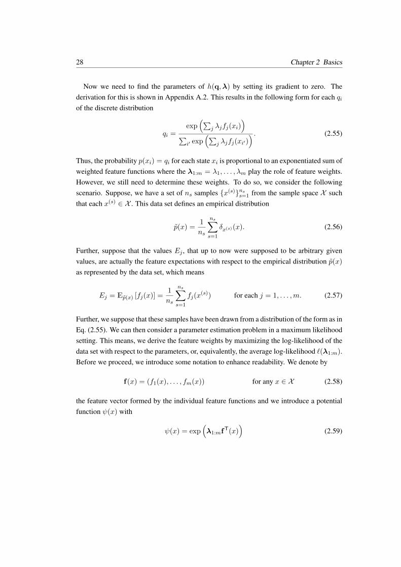
28 Chapter 2 Basics
Now we need to find the parameters of h(q,λ) by setting its gradient to zero. Thederivation for this is shown in Appendix A.2. This results in the following form for each qiof the discrete distribution
qi =exp
(∑j λjfj(xi)
)∑
i′ exp(∑
j λjfj(xi′)) . (2.55)
Thus, the probability p(xi) = qi for each state xi is proportional to an exponentiated sum ofweighted feature functions where the λ1:m = λ1, . . . , λm play the role of feature weights.However, we still need to determine these weights. To do so, we consider the followingscenario. Suppose, we have a set of ns samples x(s)nss=1 from the sample space X suchthat each x(s) ∈ X . This data set defines an empirical distribution
p(x) =1
ns
ns∑s=1
δx(s)(x). (2.56)
Further, suppose that the values Ej , that up to now were supposed to be arbitrary givenvalues, are actually the feature expectations with respect to the empirical distribution p(x)
as represented by the data set, which means
Ej = Ep(x) [fj(x)] =1
ns
ns∑s=1
fj(x(s)) for each j = 1, . . . ,m. (2.57)
Further, we suppose that these samples have been drawn from a distribution of the form as inEq. (2.55). We can then consider a parameter estimation problem in a maximum likelihoodsetting. This means, we derive the feature weights by maximizing the log-likelihood of thedata set with respect to the parameters, or, equivalently, the average log-likelihood `(λ1:m).Before we proceed, we introduce some notation to enhance readability. We denote by
f(x) = (f1(x), . . . , fm(x)) for any x ∈ X (2.58)
the feature vector formed by the individual feature functions and we introduce a potentialfunction ψ(x) with
ψ(x) = exp(λ1:mfT(x)
)(2.59)
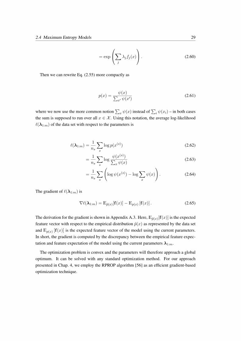
2.4 Maximum Entropy Models 29
= exp
∑j
λjfj(x)
. (2.60)
Then we can rewrite Eq. (2.55) more compactly as
p(x) =ψ(x)∑x′ ψ(x′)
(2.61)
where we now use the more common notion∑
x ψ(x) instead of∑
i ψ(xi) – in both casesthe sum is supposed to run over all x ∈ X . Using this notation, the average log-likelihood`(λ1:m) of the data set with respect to the parameters is
`(λ1:m) =1
ns
∑s
log p(x(s)) (2.62)
=1
ns
∑s
logψ(x(s))∑x ψ(x)
(2.63)
=1
ns
∑s
(logψ(x(s))− log
∑x
ψ(x)
). (2.64)
The gradient of `(λ1:m) is
∇`(λ1:m) = Ep(x)[f(x)]− Ep(x) [f(x)] . (2.65)
The derivation for the gradient is shown in Appendix A.3. Here,Ep(x)[f(x)] is the expectedfeature vector with respect to the empirical distribution p(x) as represented by the data setand Ep(x) [f(x)] is the expected feature vector of the model using the current parameters.In short, the gradient is computed by the discrepancy between the empirical feature expec-tation and feature expectation of the model using the current parameters λ1:m.
The optimization problem is convex and the parameters will therefore approach a globaloptimum. It can be solved with any standard optimization method. For our approachpresented in Chap. 4, we employ the RPROP algorithm [56] as an efficient gradient-basedoptimization technique.

30 Chapter 2 Basics
2.5 Bayesian Nonparametrics
As noted in [34], the “basic idea of Bayesian nonparametrics is to replace classical finite-dimensional prior distributions with general stochastic processes”. In this section, we givea brief introduction to three stochastic processes that are commonly used in Bayesian non-parametrics. The first two are the Dirichlet process and the beta-Bernoulli process. In thiscontext, we will also discuss hierarchical and nested extensions. The third and last processthat we discuss is the Gaussian process as used in Gaussian process regression. For a morein-depth introduction to the first two processes, we also like to refer the interested readerto the tutorials of Teh and Jordan [70] and Gershman and Blei [23]. Gaussian processregression is presented in all detail in [54].
2.5.1 Dirichlet Process and Chinese Restaurant Process
The Dirichlet process can be considered as an infinite dimensional variant of the Dirichletdistribution and a draw from it can be considered as an infinite multinomial distribution.The Dirichlet process is frequently used as a prior in mixture models in which it replacesa finite dimensional Dirichlet distribution. To help grounding the theory, and for present-ing a motivating example application, we will therefore first start with a discussion a finiteGaussian mixture models and the corresponding extension to a Dirichlet process Gaussianmixture model (DPGMM). We then give a formal definition of the Dirichlet process and,next, we illustrate an explicit representation of draws from this process by means of thestick-breaking construction. In contrast to parametric models, which have a finite numberof parameters, the Dirichlet process is a nonparametric model with infinitely many param-eters. This is problematic when we want to implement inference algorithms for modelsbased on the Dirichlet process, as we obviously cannot explicitly represent infinitely manyparameters. However, we will see that the posterior predictive distribution of the DP hasa finite dimensional representation which permits feasible algorithms for posterior infer-ence, for example in infinite mixture models. This posterior predictive distribution of aDP is closely related to the Chinese restaurant process (CRP). The connection to the DPis, that the sequential sampling of observations from the CRP can be described in terms ofsampling from a sequence of posterior predictive distributions of a DP.
The description of the Dirichlet process and related concepts in this section is mainlybased on [18, 47, 70, 71, 78] and we would like to redirect the interested reader to thesearticles for a more thorough description.

2.5 Bayesian Nonparametrics 31
2.5.1.1 Finite Gaussian Mixture Models
The Dirichlet process is often used as a prior in mixture models and it will prove usefulto keep this application in mind when we later discuss the Dirichlet process itself. In thissection, we will therefore first start with a discussion of finite Gaussian mixture models(GMM) that make use of a Dirichlet distribution as a prior over the mixture weights andwe will see that the use of a Dirichlet process prior will cause only a slight modification inthe inference procedure. This change, however, will result in a more flexible model, whichis able to adjust the number of mixture components during inference.
As a motivation, consider a scenario in which we are given a set of N points x1:N withxi ∈ Rd for some d ≥ 1 and we are interested in the predictive distribution p(x∗ | x1:N )
that models the likelihood of observing a point at a certain location x∗ given that we alreadyhave seen the points x1:N . We assume that these points have been drawn from a Gaussianmixture density p(x | β) parametrized by some β. The parameters β include the mixtureweights and the parameters of the Gaussians, but we will postpone these details for themoment. The actual form of the mixture density is unknown to us but we have a priordistribution p(β) over possible mixture densities. By observing the data points our priorover mixture densities is updated and we have a more informed posterior distribution overmixture densities
p(β | x1:N ) ∝ p(β)N∏i=1
p(xi | β). (2.66)
By marginalizing the mixture density we arrive at the posterior predictive distribution
p(x∗ | x1:N ) =
∫βp(x∗ | β)p(β | x1:N ) dβ (2.67)
which models the likelihood of a new point at location x∗ given the previously seen points.The trouble is, we might not be able solve the integral analytically. However, we can useMarkov chain Monte Carlo techniques to obtain samples β(j)Mj=1 from the posterior dis-tribution p(β | x1:N ) and compute a Monte Carlo approximation of the posterior predictivedistribution as
p(x∗ | x1:N ) ≈ 1
M
M∑j=1
p(x∗ | β(j)). (2.68)
In the following, we describe the details of how to utilize Gibbs sampling to draw sam-

32 Chapter 2 Basics
ples from the posterior distribution. We are given N data points x1:N with xi ∈ Rd thathave been sampled from a mixture density consisting of K Gaussians
xi ∼ p(· | w,µ1,Σ1, . . . ,µK ,ΣK) =K∑k=1
wkN (· | µk,Σk). (2.69)
This mixture density is parametrized by the mixture weights w = (w1, . . . , wK), whichsum to one, and the parameters of the Gaussians, i.e., their respective mean µk and co-variance matrix Σk. We will sometimes refer to the Gaussians as mixture components orclusters and refer to their parameters as cluster parameters θk = (µk,Σk). We are free tochoose any suitable prior for the latent parameters of the mixture density. In our example,we will use their respective conjugate priors and thus place a Dirichlet prior p(w) on theweights and a normal-Wishart prior p(µk,Σk) on each of the cluster parameters.
Sampling data points from the implied generative process works as follows. First, wedraw a mixture density by sampling K Gaussians from the normal-Wishart distributionand the mixture weights from a Dirichlet distribution. Given the resulting mixture density,we draw each data point xi independently by first sampling a cluster component ci ∼p(ci | w) according to the weights. Then, we sample the actual observable data pointxi ∼ N (xi | µci ,Σci) from the corresponding Gaussian ci. Please note, that we therebyintroduced correspondence variables ci ∈ 1, . . . ,K that denote the cluster from which apoint has been sampled from. For example, if c4 = 3 then point x4 has been sampled fromcluster 3. The correspondence variables are also treated as latent variables. In accordancewith the introductory remarks, we denote the latent variables by β but we now include thecorrespondence variables, so we have β = (w,θ1:K , c1:N ).
To wrap up, the generative process can be described more concisely as
w = (w1, . . . , wK) ∼ Dir(· | α) once (2.70)
θk = (µk,Σk) ∼ NW(· | ν0, κ0,µ0,T0) for k = 1, . . . ,K (2.71)
ci ∼ Mult(· | w) for i = 1, . . . , N (2.72)
xi ∼ N (· | µci ,Σci) for i = 1, . . . , N (2.73)
and the corresponding Bayesian network is depicted in Fig. 2.3.
A complete Gibbs sweep samples new values for each of the latent variables from theirrespective conditional distributions. We start with an arbitrary initial state β(0). It willprove useful to have an intuitive visualization of this state. If, as a toy example, we would

2.5 Bayesian Nonparametrics 33
α
w ν0 κ0 µ0 T0
θkci
xi
i = 1, . . . , N
k = 1, . . . ,K
Figure 2.3: Bayesian network representing a finite Gaussian mixture model.
w1 w2 w3 w4
θ1 θ2 θ3 θ4
x1
x2
x3
x4
x5
x6
Figure 2.4: A visual representation of a sample β(i).
have four Gaussians and six data points then a state β(i) of the Markov chain could bevisualized by the matrix depicted in Fig. 2.4. Here, each row corresponds to a data pointand each column corresponds to a cluster. The binary matrix visualizes the correspondencevariables, e.g. here the data point x4 is currently associated to the third Gaussian whichmeans we have c4 = 3. Further, each column is associated with the cluster variables: theparameters θk of a Gaussian and its weight wk. We now need to resample the entries of thebinary matrix, i.e., the correspondence variables, as well as the cluster parameters. For the
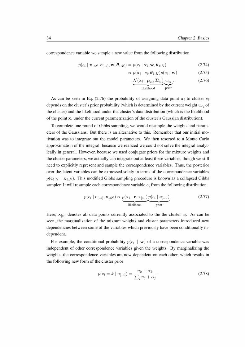
34 Chapter 2 Basics
correspondence variable we sample a new value from the following distribution
p(ci | x1:N , c[−i],w,θ1:K) = p(ci | xi,w,θ1:K) (2.74)
∝ p(xi | ci,θ1:K)p(ci | w) (2.75)
= N (xi | µci ,Σci)︸ ︷︷ ︸likelihood
wci︸︷︷︸prior
. (2.76)
As can be seen in Eq. (2.76) the probability of assigning data point xi to cluster cidepends on the cluster’s prior probability (which is determined by the current weight wci ofthe cluster) and the likelihood under the cluster’s data distribution (which is the likelihoodof the point xi under the current parametrization of the cluster’s Gaussian distribution).
To complete one round of Gibbs sampling, we would resample the weights and param-eters of the Gaussians. But there is an alternative to this. Remember that our initial mo-tivation was to integrate out the model parameters. We then resorted to a Monte Carloapproximation of the integral, because we realized we could not solve the integral analyt-ically in general. However, because we used conjugate priors for the mixture weights andthe cluster parameters, we actually can integrate out at least these variables, though we stillneed to explicitly represent and sample the correspondence variables. Thus, the posteriorover the latent variables can be expressed solely in terms of the correspondence variablesp(c1:N | x1:N ). This modified Gibbs sampling procedure is known as a collapsed Gibbssampler. It will resample each correspondence variable ci from the following distribution
p(ci | c[−i],x1:N ) ∝ p(xi | c,x[ci])︸ ︷︷ ︸likelihood
p(ci | c[−i])︸ ︷︷ ︸prior
. (2.77)
Here, x[ci] denotes all data points currently associated to the the cluster ci. As can beseen, the marginalization of the mixture weights and cluster parameters introduced newdependencies between some of the variables which previously have been conditionally in-dependent.
For example, the conditional probability p(ci | w) of a correspondence variable wasindependent of other correspondence variables given the weights. By marginalizing theweights, the correspondence variables are now dependent on each other, which results inthe following new form of the cluster prior
p(ci = k | c[−i]) =nk + αk∑j nj + αj
. (2.78)
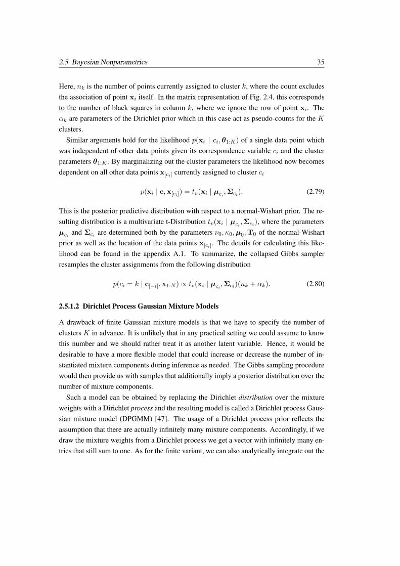
2.5 Bayesian Nonparametrics 35
Here, nk is the number of points currently assigned to cluster k, where the count excludesthe association of point xi itself. In the matrix representation of Fig. 2.4, this correspondsto the number of black squares in column k, where we ignore the row of point xi. Theαk are parameters of the Dirichlet prior which in this case act as pseudo-counts for the Kclusters.
Similar arguments hold for the likelihood p(xi | ci,θ1:K) of a single data point whichwas independent of other data points given its correspondence variable ci and the clusterparameters θ1:K . By marginalizing out the cluster parameters the likelihood now becomesdependent on all other data points x[ci] currently assigned to cluster ci
p(xi | c,x[ci]) = tv(xi | µci ,Σci). (2.79)
This is the posterior predictive distribution with respect to a normal-Wishart prior. The re-sulting distribution is a multivariate t-Distribution tv(xi | µci ,Σci), where the parametersµci and Σci are determined both by the parameters ν0, κ0,µ0,T0 of the normal-Wishartprior as well as the location of the data points x[ci]. The details for calculating this like-lihood can be found in the appendix A.1. To summarize, the collapsed Gibbs samplerresamples the cluster assignments from the following distribution
p(ci = k | c[−i],x1:N ) ∝ tv(xi | µci ,Σci)(nk + αk). (2.80)
2.5.1.2 Dirichlet Process Gaussian Mixture Models
A drawback of finite Gaussian mixture models is that we have to specify the number ofclusters K in advance. It is unlikely that in any practical setting we could assume to knowthis number and we should rather treat it as another latent variable. Hence, it would bedesirable to have a more flexible model that could increase or decrease the number of in-stantiated mixture components during inference as needed. The Gibbs sampling procedurewould then provide us with samples that additionally imply a posterior distribution over thenumber of mixture components.
Such a model can be obtained by replacing the Dirichlet distribution over the mixtureweights with a Dirichlet process and the resulting model is called a Dirichlet process Gaus-sian mixture model (DPGMM) [47]. The usage of a Dirichlet process prior reflects theassumption that there are actually infinitely many mixture components. Accordingly, if wedraw the mixture weights from a Dirichlet process we get a vector with infinitely many en-tries that still sum to one. As for the finite variant, we can also analytically integrate out the
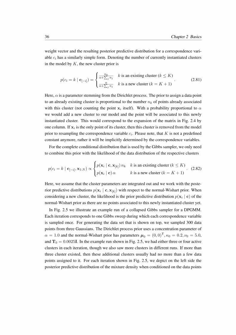
36 Chapter 2 Basics
weight vector and the resulting posterior predictive distribution for a correspondence vari-able ci has a similarly simple form. Denoting the number of currently instantiated clustersin the model by K, the new cluster prior is
p(ci = k | c[−i]) =
nk
α+∑j nj
k is an existing cluster (k ≤ K)
αα+
∑j nj
k is a new cluster (k = K + 1). (2.81)
Here, α is a parameter stemming from the Dirichlet process. The prior to assign a data pointto an already existing cluster is proportional to the number nk of points already associatedwith this cluster (not counting the point xi itself). With a probability proportional to αwe would add a new cluster to our model and the point will be associated to this newlyinstantiated cluster. This would correspond to the expansion of the matrix in Fig. 2.4 byone column. If xi is the only point of its cluster, then this cluster is removed from the modelprior to resampling the correspondence variable ci. Please note, that K is not a predefinedconstant anymore, rather it will be implicitly determined by the correspondence variables.
For the complete conditional distribution that is used by the Gibbs sampler, we only needto combine this prior with the likelihood of the data distribution of the respective clusters
p(ci = k | c[−i],x1:N ) ∝
p(xi | c,x[k])nk k is an existing cluster (k ≤ K)
p(xi | c)α k is a new cluster (k = K + 1). (2.82)
Here, we assume that the cluster parameters are integrated out and we work with the poste-rior predictive distributions p(xi | c,x[k]) with respect to the normal-Wishart prior. Whenconsidering a new cluster, the likelihood is the prior predictive distribution p(xi | c) of thenormal-Wishart prior as there are no points associated to this newly instantiated cluster yet.
In Fig. 2.5 we illustrate an example run of a collapsed Gibbs sampler for a DPGMM.Each iteration corresponds to one Gibbs sweep during which each correspondence variableis sampled once. For generating the data set that is shown on top, we sampled 300 datapoints from three Gaussians. The Dirichlet process prior uses a concentration parameter ofα = 1.0 and the normal-Wishart prior has parameters µ0 = (0, 0)T, κ0 = 0.2, ν0 = 5.0,and T0 = 0.0025I. In the example run shown in Fig. 2.5, we had either three or four activeclusters in each iteration, though we also saw more clusters in different runs. If more thanthree cluster existed, then these additional clusters usually had no more than a few datapoints assigned to it. For each iteration shown in Fig. 2.5, we depict on the left side theposterior predictive distribution of the mixture density when conditioned on the data points
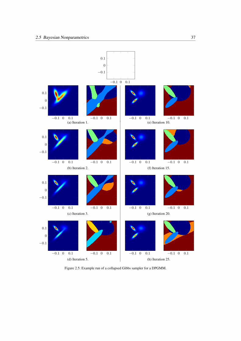
2.5 Bayesian Nonparametrics 37
−0.1 0 0.1
−0.1
0
0.1
−0.1 0 0.1
−0.1
0
0.1
−0.1 0 0.1 −0.1 0 0.1 −0.1 0 0.1(a) Iteration 1. (e) Iteration 10.
−0.1 0 0.1
−0.1
0
0.1
−0.1 0 0.1 −0.1 0 0.1 −0.1 0 0.1
(b) Iteration 2. (f) Iteration 15.
−0.1 0 0.1
−0.1
0
0.1
−0.1 0 0.1 −0.1 0 0.1 −0.1 0 0.1
(c) Iteration 3. (g) Iteration 20.
−0.1 0 0.1
−0.1
0
0.1
−0.1 0 0.1 −0.1 0 0.1 −0.1 0 0.1
(d) Iteration 5. (h) Iteration 25.
Figure 2.5: Example run of a collapsed Gibbs sampler for a DPGMM.
38 Chapter 2 Basics
with their current cluster assignments. On the right side, we depict the most likely clusterassignment for a new point. Any new point that falls into the red area would most likely beassigned to a newly instantiated cluster.
We have seen, that this sampling technique can increase or decrease the number of com-ponents in the mixture model, which allows the effective model complexity to adapt to thedata complexity as needed. Hence, this gives us the desired flexibility of not having tospecify the number of components in advance. We now rather have a prior over the numberof components which is influenced by the parameter α. The higher α the more componentswe expect a priori. Posterior inference in this model remains tractable, even though weassume that there exist infinitely many mixture components, because we only have to con-sider the currently instantiated clusters plus the possibility of expanding the model with oneadditional cluster. This makes the model also appealing from a computational perspective.In the following, we will discuss the Dirichlet process in more detail.
2.5.1.3 Definition of the Dirichlet Process
The Dirichlet process was introduced by Ferguson [18]. It can be defined as follows.1 LetG0 be a distribution over the sample space Ω, and let α > 0 be a positive real number. Thena random distribution G over the sample space Ω is distributed according to a Dirichletprocess with concentration parameter α and base distribution G0
G ∼ DP(α,G0), (2.83)
if for all k ≥ 1 and all partitions (A1, . . . , Ak) of Ω the vector (G(A1), . . . , G(Ak)) isDirichlet distributed according to
(G(A1), . . . , G(Ak)) ∼ Dir(αG0(A1), . . . , αG0(Ak)). (2.84)
The intuition behind Eq. (2.84) will become more apparent in the next section when welook at an explicit representation for a draw G.
2.5.1.4 Stick-breaking Construction
The definition of the Dirichlet process as given above was not a constructive one. It didnot provide us with any means to actually draw a distribution G that satisfies these require-
1This is a slightly simplified definition that avoids measure theoretic jargon.
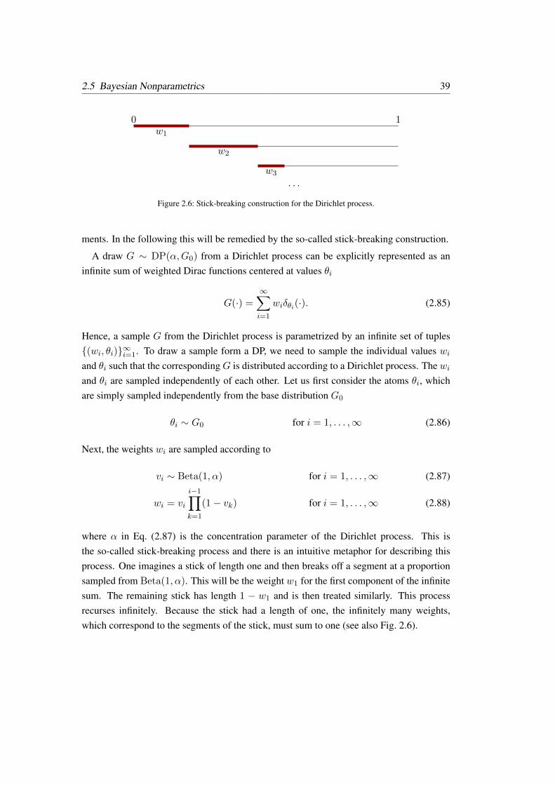
2.5 Bayesian Nonparametrics 39
0 1w1
w2
w3
. . .
Figure 2.6: Stick-breaking construction for the Dirichlet process.
ments. In the following this will be remedied by the so-called stick-breaking construction.
A draw G ∼ DP(α,G0) from a Dirichlet process can be explicitly represented as aninfinite sum of weighted Dirac functions centered at values θi
G(·) =∞∑i=1
wiδθi(·). (2.85)
Hence, a sample G from the Dirichlet process is parametrized by an infinite set of tuples(wi, θi)∞i=1. To draw a sample form a DP, we need to sample the individual values wiand θi such that the correspondingG is distributed according to a Dirichlet process. The wiand θi are sampled independently of each other. Let us first consider the atoms θi, whichare simply sampled independently from the base distribution G0
θi ∼ G0 for i = 1, . . . ,∞ (2.86)
Next, the weights wi are sampled according to
vi ∼ Beta(1, α) for i = 1, . . . ,∞ (2.87)
wi = vi
i−1∏k=1
(1− vk) for i = 1, . . . ,∞ (2.88)
where α in Eq. (2.87) is the concentration parameter of the Dirichlet process. This isthe so-called stick-breaking process and there is an intuitive metaphor for describing thisprocess. One imagines a stick of length one and then breaks off a segment at a proportionsampled from Beta(1, α). This will be the weight w1 for the first component of the infinitesum. The remaining stick has length 1 − w1 and is then treated similarly. This processrecurses infinitely. Because the stick had a length of one, the infinitely many weights,which correspond to the segments of the stick, must sum to one (see also Fig. 2.6).
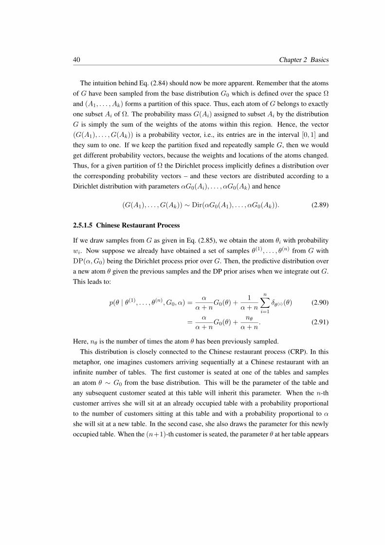
40 Chapter 2 Basics
The intuition behind Eq. (2.84) should now be more apparent. Remember that the atomsof G have been sampled from the base distribution G0 which is defined over the space Ω
and (A1, . . . , Ak) forms a partition of this space. Thus, each atom of G belongs to exactlyone subset Ai of Ω. The probability mass G(Ai) assigned to subset Ai by the distributionG is simply the sum of the weights of the atoms within this region. Hence, the vector(G(A1), . . . , G(Ak)) is a probability vector, i.e., its entries are in the interval [0, 1] andthey sum to one. If we keep the partition fixed and repeatedly sample G, then we wouldget different probability vectors, because the weights and locations of the atoms changed.Thus, for a given partition of Ω the Dirichlet process implicitly defines a distribution overthe corresponding probability vectors – and these vectors are distributed according to aDirichlet distribution with parameters αG0(Ai), . . . , αG0(Ak) and hence
(G(A1), . . . , G(Ak)) ∼ Dir(αG0(A1), . . . , αG0(Ak)). (2.89)
2.5.1.5 Chinese Restaurant Process
If we draw samples from G as given in Eq. (2.85), we obtain the atom θi with probabilitywi. Now suppose we already have obtained a set of samples θ(1), . . . , θ(n) from G withDP(α,G0) being the Dirichlet process prior over G. Then, the predictive distribution overa new atom θ given the previous samples and the DP prior arises when we integrate out G.This leads to:
p(θ | θ(1), . . . , θ(n), G0, α) =α
α+ nG0(θ) +
1
α+ n
n∑i=1
δθ(i)(θ) (2.90)
=α
α+ nG0(θ) +
nθα+ n
. (2.91)
Here, nθ is the number of times the atom θ has been previously sampled.This distribution is closely connected to the Chinese restaurant process (CRP). In this
metaphor, one imagines customers arriving sequentially at a Chinese restaurant with aninfinite number of tables. The first customer is seated at one of the tables and samplesan atom θ ∼ G0 from the base distribution. This will be the parameter of the table andany subsequent customer seated at this table will inherit this parameter. When the n-thcustomer arrives she will sit at an already occupied table with a probability proportionalto the number of customers sitting at this table and with a probability proportional to αshe will sit at a new table. In the second case, she also draws the parameter for this newlyoccupied table. When the (n+1)-th customer is seated, the parameter θ at her table appears
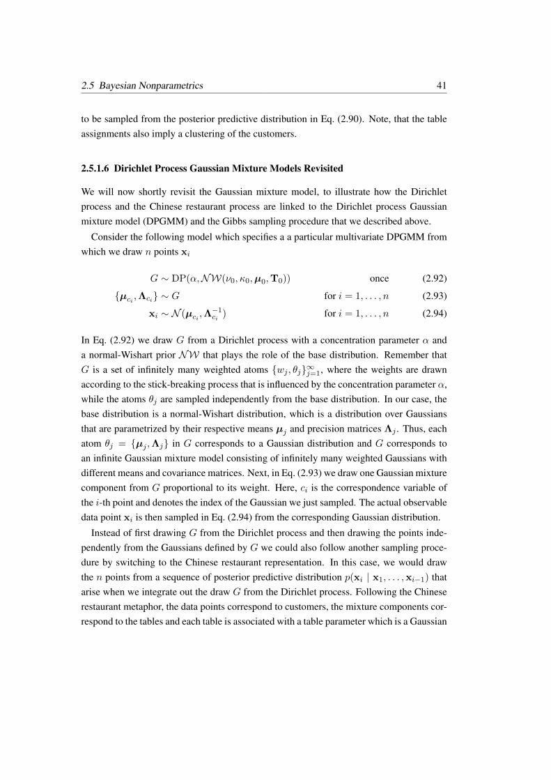
2.5 Bayesian Nonparametrics 41
to be sampled from the posterior predictive distribution in Eq. (2.90). Note, that the tableassignments also imply a clustering of the customers.
2.5.1.6 Dirichlet Process Gaussian Mixture Models Revisited
We will now shortly revisit the Gaussian mixture model, to illustrate how the Dirichletprocess and the Chinese restaurant process are linked to the Dirichlet process Gaussianmixture model (DPGMM) and the Gibbs sampling procedure that we described above.
Consider the following model which specifies a a particular multivariate DPGMM fromwhich we draw n points xi
G ∼ DP(α,NW(ν0, κ0,µ0,T0)) once (2.92)
µci ,Λci ∼ G for i = 1, . . . , n (2.93)
xi ∼ N (µci ,Λ−1ci ) for i = 1, . . . , n (2.94)
In Eq. (2.92) we draw G from a Dirichlet process with a concentration parameter α anda normal-Wishart prior NW that plays the role of the base distribution. Remember thatG is a set of infinitely many weighted atoms wj , θj∞j=1, where the weights are drawnaccording to the stick-breaking process that is influenced by the concentration parameter α,while the atoms θj are sampled independently from the base distribution. In our case, thebase distribution is a normal-Wishart distribution, which is a distribution over Gaussiansthat are parametrized by their respective means µj and precision matrices Λj . Thus, eachatom θj = µj ,Λj in G corresponds to a Gaussian distribution and G corresponds toan infinite Gaussian mixture model consisting of infinitely many weighted Gaussians withdifferent means and covariance matrices. Next, in Eq. (2.93) we draw one Gaussian mixturecomponent from G proportional to its weight. Here, ci is the correspondence variable ofthe i-th point and denotes the index of the Gaussian we just sampled. The actual observabledata point xi is then sampled in Eq. (2.94) from the corresponding Gaussian distribution.
Instead of first drawing G from the Dirichlet process and then drawing the points inde-pendently from the Gaussians defined by G we could also follow another sampling proce-dure by switching to the Chinese restaurant representation. In this case, we would drawthe n points from a sequence of posterior predictive distribution p(xi | x1, . . . ,xi−1) thatarise when we integrate out the draw G from the Dirichlet process. Following the Chineserestaurant metaphor, the data points correspond to customers, the mixture components cor-respond to the tables and each table is associated with a table parameter which is a Gaussian
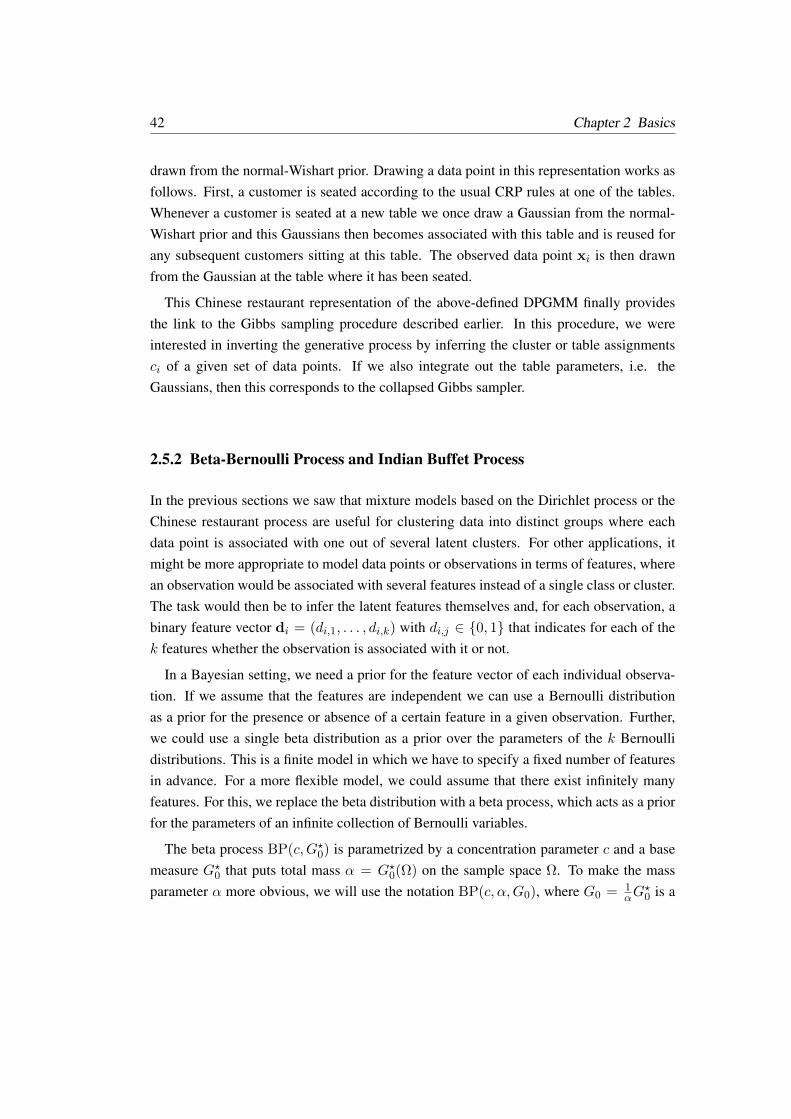
42 Chapter 2 Basics
drawn from the normal-Wishart prior. Drawing a data point in this representation works asfollows. First, a customer is seated according to the usual CRP rules at one of the tables.Whenever a customer is seated at a new table we once draw a Gaussian from the normal-Wishart prior and this Gaussians then becomes associated with this table and is reused forany subsequent customers sitting at this table. The observed data point xi is then drawnfrom the Gaussian at the table where it has been seated.
This Chinese restaurant representation of the above-defined DPGMM finally providesthe link to the Gibbs sampling procedure described earlier. In this procedure, we wereinterested in inverting the generative process by inferring the cluster or table assignmentsci of a given set of data points. If we also integrate out the table parameters, i.e. theGaussians, then this corresponds to the collapsed Gibbs sampler.
2.5.2 Beta-Bernoulli Process and Indian Buffet Process
In the previous sections we saw that mixture models based on the Dirichlet process or theChinese restaurant process are useful for clustering data into distinct groups where eachdata point is associated with one out of several latent clusters. For other applications, itmight be more appropriate to model data points or observations in terms of features, wherean observation would be associated with several features instead of a single class or cluster.The task would then be to infer the latent features themselves and, for each observation, abinary feature vector di = (di,1, . . . , di,k) with di,j ∈ 0, 1 that indicates for each of thek features whether the observation is associated with it or not.
In a Bayesian setting, we need a prior for the feature vector of each individual observa-tion. If we assume that the features are independent we can use a Bernoulli distributionas a prior for the presence or absence of a certain feature in a given observation. Further,we could use a single beta distribution as a prior over the parameters of the k Bernoullidistributions. This is a finite model in which we have to specify a fixed number of featuresin advance. For a more flexible model, we could assume that there exist infinitely manyfeatures. For this, we replace the beta distribution with a beta process, which acts as a priorfor the parameters of an infinite collection of Bernoulli variables.
The beta process BP(c,G?0) is parametrized by a concentration parameter c and a basemeasure G?0 that puts total mass α = G?0(Ω) on the sample space Ω. To make the massparameter α more obvious, we will use the notation BP(c, α,G0), where G0 = 1
αG?0 is a
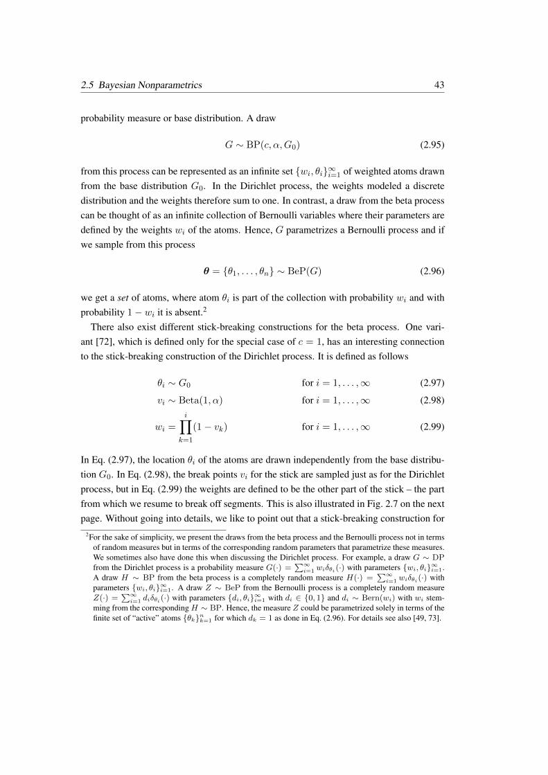
2.5 Bayesian Nonparametrics 43
probability measure or base distribution. A draw
G ∼ BP(c, α,G0) (2.95)
from this process can be represented as an infinite set wi, θi∞i=1 of weighted atoms drawnfrom the base distribution G0. In the Dirichlet process, the weights modeled a discretedistribution and the weights therefore sum to one. In contrast, a draw from the beta processcan be thought of as an infinite collection of Bernoulli variables where their parameters aredefined by the weights wi of the atoms. Hence, G parametrizes a Bernoulli process and ifwe sample from this process
θ = θ1, . . . , θn ∼ BeP(G) (2.96)
we get a set of atoms, where atom θi is part of the collection with probability wi and withprobability 1− wi it is absent.2
There also exist different stick-breaking constructions for the beta process. One vari-ant [72], which is defined only for the special case of c = 1, has an interesting connectionto the stick-breaking construction of the Dirichlet process. It is defined as follows
θi ∼ G0 for i = 1, . . . ,∞ (2.97)
vi ∼ Beta(1, α) for i = 1, . . . ,∞ (2.98)
wi =i∏
k=1
(1− vk) for i = 1, . . . ,∞ (2.99)
In Eq. (2.97), the location θi of the atoms are drawn independently from the base distribu-tion G0. In Eq. (2.98), the break points vi for the stick are sampled just as for the Dirichletprocess, but in Eq. (2.99) the weights are defined to be the other part of the stick – the partfrom which we resume to break off segments. This is also illustrated in Fig. 2.7 on the nextpage. Without going into details, we like to point out that a stick-breaking construction for
2For the sake of simplicity, we present the draws from the beta process and the Bernoulli process not in termsof random measures but in terms of the corresponding random parameters that parametrize these measures.We sometimes also have done this when discussing the Dirichlet process. For example, a draw G ∼ DPfrom the Dirichlet process is a probability measure G(·) =
∑∞i=1 wiδθi(·) with parameters wi, θi∞i=1.
A draw H ∼ BP from the beta process is a completely random measure H(·) =∑∞i=1 wiδθi(·) with
parameters wi, θi∞i=1. A draw Z ∼ BeP from the Bernoulli process is a completely random measureZ(·) =
∑∞i=1 diδθi(·) with parameters di, θi∞i=1 with di ∈ 0, 1 and di ∼ Bern(wi) with wi stem-
ming from the correspondingH ∼ BP. Hence, the measure Z could be parametrized solely in terms of thefinite set of “active” atoms θknk=1 for which dk = 1 as done in Eq. (2.96). For details see also [49, 73].
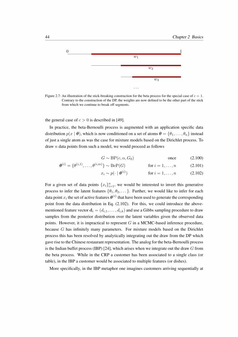
44 Chapter 2 Basics
0 1w1
w2
w3
. . .
Figure 2.7: An illustration of the stick-breaking construction for the beta process for the special case of c = 1.Contrary to the construction of the DP, the weights are now defined to be the other part of the stickfrom which we continue to break off segments.
the general case of c > 0 is described in [49].
In practice, the beta-Bernoulli process is augmented with an application specific datadistribution p(x | θ), which is now conditioned on a set of atoms θ = θ1, . . . , θn insteadof just a single atom as was the case for mixture models based on the Dirichlet process. Todraw n data points from such a model, we would proceed as follows
G ∼ BP(c, α,G0) once (2.100)
θ(i) = θ(i,1), . . . , θ(i,m) ∼ BeP(G) for i = 1, . . . , n (2.101)
xi ∼ p(· | θ(i)) for i = 1, . . . , n (2.102)
For a given set of data points xini=1, we would be interested to invert this generativeprocess to infer the latent features θ1, θ2, . . . . Further, we would like to infer for eachdata point xi the set of active features θ(i) that have been used to generate the correspondingpoint from the data distribution in Eq. (2.102). For this, we could introduce the above-mentioned feature vector di = (di,1, . . . , di,k) and use a Gibbs sampling procedure to drawsamples from the posterior distribution over the latent variables given the observed datapoints. However, it is impractical to represent G in a MCMC-based inference procedure,because G has infinitely many parameters. For mixture models based on the Dirichletprocess this has been resolved by analytically integrating out the draw from the DP whichgave rise to the Chinese restaurant representation. The analog for the beta-Bernoulli processis the Indian buffet process (IBP) [24], which arises when we integrate out the drawG fromthe beta process. While in the CRP a customer has been associated to a single class (ortable), in the IBP a customer would be associated to multiple features (or dishes).
More specifically, in the IBP metaphor one imagines customers arriving sequentially at

2.5 Bayesian Nonparametrics 45
an Indian buffet with an infinite number of dishes where each dish is associated with a dishparameter θ sampled from the base distribution G0. The first customer at the buffet tastesa certain number of dishes and this number n1,+ is drawn from a Poisson distribution withmean α
n1,+ ∼ Pois (α) , (2.103)
where α is the mass parameter of the beta process. The i-th customer arriving at the buffettastes some of the dishes that previous customers have tasted already, as well as a certainnumber of new dishes. The previously chosen dishes are selected based on their popularity,that is, with a probability of
nki− 1 + c
(2.104)
the i-th customer also tastes dish k, where nk ≥ 1 is the number of customers that pre-viously selected dish k. Here, c is the concentration parameter of the beta process. Thisdecision is made independently for each of the previously tasted dishes, which reflects thefact that the atoms of G model independent Bernoulli variables. The i-th customer thenadditionally tastes a Poisson distributed number ni,+ of new dishes not chosen by any cus-tomer before her
ni,+ ∼ Pois
(cα
i− 1 + c
). (2.105)
This also includes the possibility of not choosing any new dishes at all. Whenever a dish hasbeen tasted for the first time, we once sample its associated dish parameter θ from the basedistribution G0. This is the two-parameter IBP introduced in [73]. The original IBP [24] isrecovered with c = 1. Further, we like to point out that a three parameter generalization ofthe IBP has been proposed in [69].
We could then use the IBP representation for a Gibbs sampler that resamples the dishassignments for each customer. As with the CRP, during Gibbs sampling one can assumethat any customer is the last one to arrive at the buffet and resample the dish assignmentsaccordingly. The data likelihood of a customer (data point) then depends on the associateddish parameters of all dishes she has tasted. Similar as for the CRP, a state of the Gibbssampler can be visualized by the corresponding association matrix shown in Fig. 2.8 on thenext page. The rows correspond to the dishes of the buffet and the rows to the customers.Please note, that in contrast to the CRP, a row may now contain multiple black squares (as-sociations). If the data distribution is conjugate to the base distribution of the beta process,then the dish parameters can be integrated out analytically and do not have to be explicitlyrepresented during Gibbs sampling. However, depending on the application, for the IBP
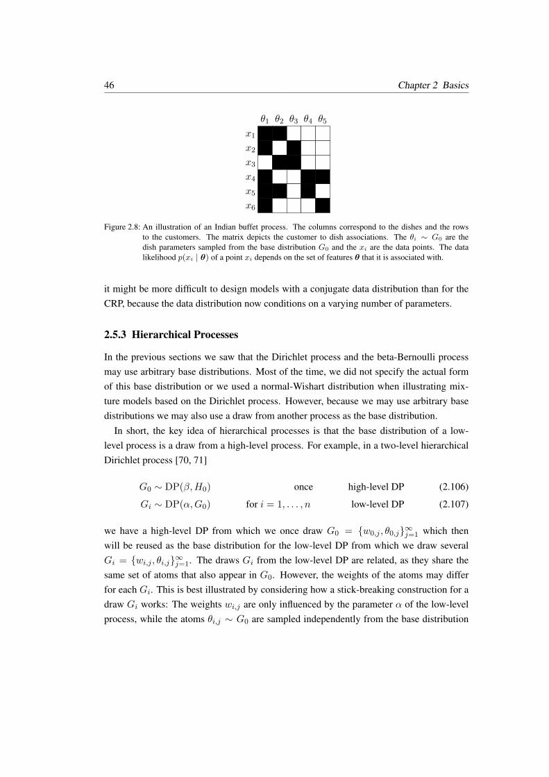
46 Chapter 2 Basics
θ1 θ2 θ3 θ4 θ5
x1
x2
x3
x4
x5
x6
Figure 2.8: An illustration of an Indian buffet process. The columns correspond to the dishes and the rowsto the customers. The matrix depicts the customer to dish associations. The θi ∼ G0 are thedish parameters sampled from the base distribution G0 and the xi are the data points. The datalikelihood p(xi | θ) of a point xi depends on the set of features θ that it is associated with.
it might be more difficult to design models with a conjugate data distribution than for theCRP, because the data distribution now conditions on a varying number of parameters.
2.5.3 Hierarchical Processes
In the previous sections we saw that the Dirichlet process and the beta-Bernoulli processmay use arbitrary base distributions. Most of the time, we did not specify the actual formof this base distribution or we used a normal-Wishart distribution when illustrating mix-ture models based on the Dirichlet process. However, because we may use arbitrary basedistributions we may also use a draw from another process as the base distribution.
In short, the key idea of hierarchical processes is that the base distribution of a low-level process is a draw from a high-level process. For example, in a two-level hierarchicalDirichlet process [70, 71]
G0 ∼ DP(β,H0) once high-level DP (2.106)
Gi ∼ DP(α,G0) for i = 1, . . . , n low-level DP (2.107)
we have a high-level DP from which we once draw G0 = w0,j , θ0,j∞j=1 which thenwill be reused as the base distribution for the low-level DP from which we draw severalGi = wi,j , θi,j∞j=1. The draws Gi from the low-level DP are related, as they share thesame set of atoms that also appear in G0. However, the weights of the atoms may differfor each Gi. This is best illustrated by considering how a stick-breaking construction for adraw Gi works: The weights wi,j are only influenced by the parameter α of the low-levelprocess, while the atoms θi,j ∼ G0 are sampled independently from the base distribution
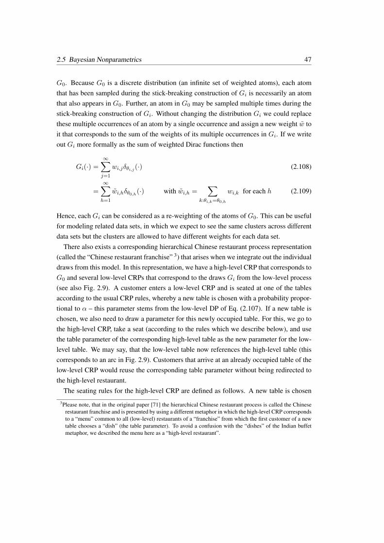
2.5 Bayesian Nonparametrics 47
G0. Because G0 is a discrete distribution (an infinite set of weighted atoms), each atomthat has been sampled during the stick-breaking construction of Gi is necessarily an atomthat also appears in G0. Further, an atom in G0 may be sampled multiple times during thestick-breaking construction of Gi. Without changing the distribution Gi we could replacethese multiple occurrences of an atom by a single occurrence and assign a new weight w toit that corresponds to the sum of the weights of its multiple occurrences in Gi. If we writeout Gi more formally as the sum of weighted Dirac functions then
Gi(·) =∞∑j=1
wi,jδθi,j (·) (2.108)
=
∞∑h=1
wi,hδθ0,h(·) with wi,h =∑
k:θi,k=θ0,h
wi,k for each h (2.109)
Hence, each Gi can be considered as a re-weighting of the atoms of G0. This can be usefulfor modeling related data sets, in which we expect to see the same clusters across differentdata sets but the clusters are allowed to have different weights for each data set.
There also exists a corresponding hierarchical Chinese restaurant process representation(called the “Chinese restaurant franchise” 3) that arises when we integrate out the individualdraws from this model. In this representation, we have a high-level CRP that corresponds toG0 and several low-level CRPs that correspond to the draws Gi from the low-level process(see also Fig. 2.9). A customer enters a low-level CRP and is seated at one of the tablesaccording to the usual CRP rules, whereby a new table is chosen with a probability propor-tional to α – this parameter stems from the low-level DP of Eq. (2.107). If a new table ischosen, we also need to draw a parameter for this newly occupied table. For this, we go tothe high-level CRP, take a seat (according to the rules which we describe below), and usethe table parameter of the corresponding high-level table as the new parameter for the low-level table. We may say, that the low-level table now references the high-level table (thiscorresponds to an arc in Fig. 2.9). Customers that arrive at an already occupied table of thelow-level CRP would reuse the corresponding table parameter without being redirected tothe high-level restaurant.
The seating rules for the high-level CRP are defined as follows. A new table is chosen
3Please note, that in the original paper [71] the hierarchical Chinese restaurant process is called the Chineserestaurant franchise and is presented by using a different metaphor in which the high-level CRP correspondsto a “menu” common to all (low-level) restaurants of a “franchise” from which the first customer of a newtable chooses a “dish” (the table parameter). To avoid a confusion with the “dishes” of the Indian buffetmetaphor, we described the menu here as a “high-level restaurant”.
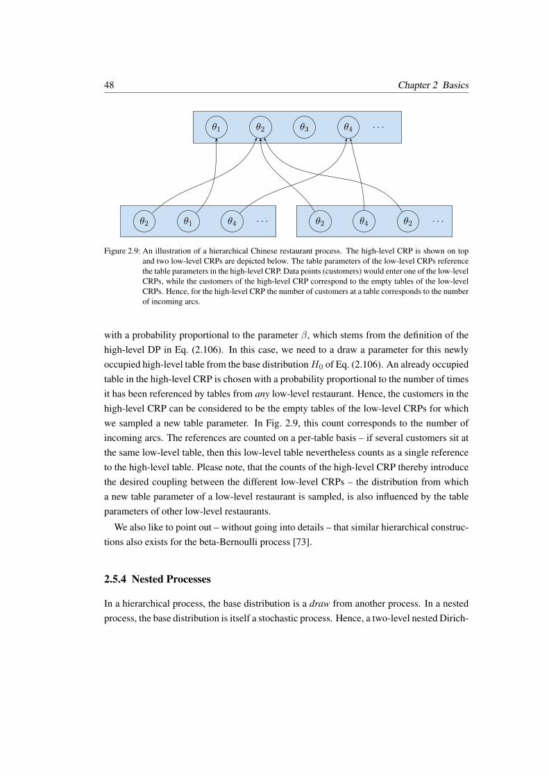
48 Chapter 2 Basics
θ1 θ2 θ3 θ4. . .
θ2 θ1 θ4. . . θ2 θ4 θ2
. . .
Figure 2.9: An illustration of a hierarchical Chinese restaurant process. The high-level CRP is shown on topand two low-level CRPs are depicted below. The table parameters of the low-level CRPs referencethe table parameters in the high-level CRP. Data points (customers) would enter one of the low-levelCRPs, while the customers of the high-level CRP correspond to the empty tables of the low-levelCRPs. Hence, for the high-level CRP the number of customers at a table corresponds to the numberof incoming arcs.
with a probability proportional to the parameter β, which stems from the definition of thehigh-level DP in Eq. (2.106). In this case, we need to a draw a parameter for this newlyoccupied high-level table from the base distributionH0 of Eq. (2.106). An already occupiedtable in the high-level CRP is chosen with a probability proportional to the number of timesit has been referenced by tables from any low-level restaurant. Hence, the customers in thehigh-level CRP can be considered to be the empty tables of the low-level CRPs for whichwe sampled a new table parameter. In Fig. 2.9, this count corresponds to the number ofincoming arcs. The references are counted on a per-table basis – if several customers sit atthe same low-level table, then this low-level table nevertheless counts as a single referenceto the high-level table. Please note, that the counts of the high-level CRP thereby introducethe desired coupling between the different low-level CRPs – the distribution from whicha new table parameter of a low-level restaurant is sampled, is also influenced by the tableparameters of other low-level restaurants.
We also like to point out – without going into details – that similar hierarchical construc-tions also exists for the beta-Bernoulli process [73].
2.5.4 Nested Processes
In a hierarchical process, the base distribution is a draw from another process. In a nestedprocess, the base distribution is itself a stochastic process. Hence, a two-level nested Dirich-
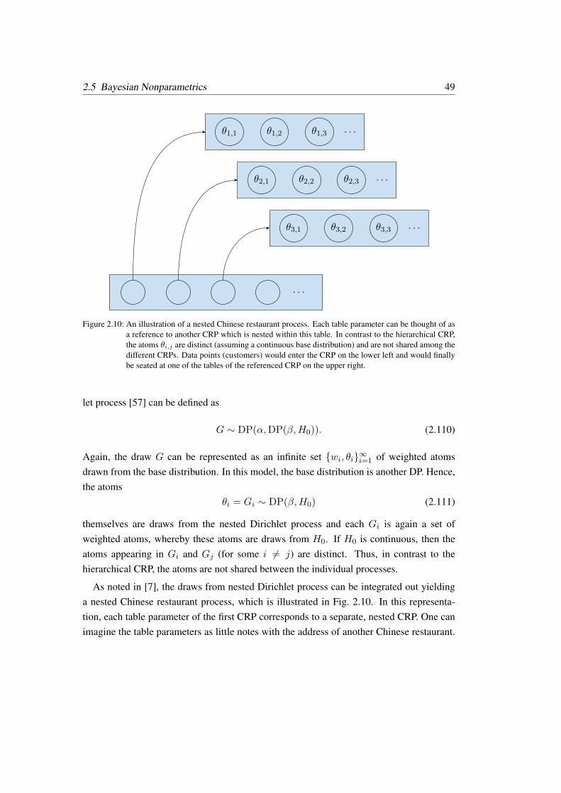
2.5 Bayesian Nonparametrics 49
. . .
θ1,1 θ1,2 θ1,3 . . .
θ2,1 θ2,2 θ2,3 . . .
θ3,1 θ3,2 θ3,3 . . .
Figure 2.10: An illustration of a nested Chinese restaurant process. Each table parameter can be thought of asa reference to another CRP which is nested within this table. In contrast to the hierarchical CRP,the atoms θi,j are distinct (assuming a continuous base distribution) and are not shared among thedifferent CRPs. Data points (customers) would enter the CRP on the lower left and would finallybe seated at one of the tables of the referenced CRP on the upper right.
let process [57] can be defined as
G ∼ DP(α,DP(β,H0)). (2.110)
Again, the draw G can be represented as an infinite set wi, θi∞i=1 of weighted atomsdrawn from the base distribution. In this model, the base distribution is another DP. Hence,the atoms
θi = Gi ∼ DP(β,H0) (2.111)
themselves are draws from the nested Dirichlet process and each Gi is again a set ofweighted atoms, whereby these atoms are draws from H0. If H0 is continuous, then theatoms appearing in Gi and Gj (for some i 6= j) are distinct. Thus, in contrast to thehierarchical CRP, the atoms are not shared between the individual processes.
As noted in [7], the draws from nested Dirichlet process can be integrated out yieldinga nested Chinese restaurant process, which is illustrated in Fig. 2.10. In this representa-tion, each table parameter of the first CRP corresponds to a separate, nested CRP. One canimagine the table parameters as little notes with the address of another Chinese restaurant.
50 Chapter 2 Basics
A customer arriving at a table of the first restaurant is transferred to the referenced secondrestaurant and is finally seated there. A Gibbs sampler for such a model needs to maintainand resample two association variables for each data point (or customer): one index for thetable in the first restaurant and a second index for the table in the referenced restaurant.This model can also be extended to multiple levels in the obvious way.
Nested models therefore separate data points into distinct non-interacting groups andeach group maintains its own set of atoms. In contrast, hierarchical models promote thesharing of information among low-level processes by maintaining a globally available setof atoms that can be referenced from the various low-level processes.
The Dirichlet process and the beta process can also be mixed in such models. For exam-ple, a beta process can be the base distribution in a Dirichlet process. In the usual metaphor,a customer arriving at a table in the Chinese restaurant would be transferred to an Indianrestaurant with a large buffet, where she tastes different dishes. A draw from such a modelwould result in a set of atoms:
G ∼ DP(α,BP(c, β,H0)) (2.112)
G(i) ∼ G (2.113)
θ(i,1), . . . , θ(i,k) ∼ BeP(G(i)) (2.114)
2.5.5 Gaussian Process Regression
The Dirichlet process and the beta process place a prior on discrete structures representedby an infinite set of weighted atoms. In Gaussian process regression, we place a prior oncontinuous functions. This is useful for regression, in which we are given a set of pointsand are interested in the posterior distribution over functions that are consistent with ourobservations. Based on this posterior distribution we can evaluate the predictive likelihoodfor observing a point at a new location given the previously seen data points.
More formally, in Gaussian process regression [54], we are given a set (xi, yi)ni=1 ofnoisy observations yi = f(xi) + ε of an unknown function f : Rn → R evaluated atinput locations xi. The additive noise ε is assumed to be Gaussian ε ∼ N (0, σ2
n) with zeromean and variance σ2
n. The objective is to estimate the function value f(x∗) at an arbitrarylocation x∗ given the data D = (xi, yi)ni=1.
Gaussian processes (GPs) are a nonparametric approach to the regression problem, thatis, we do not have to specify a parametric form of the unknown function f and fit thefunction parameters to the data. Instead, a GP can be considered as a distribution over
2.5 Bayesian Nonparametrics 51
functions. A GP is specified by a mean function m(·) and covariance function k(·, ·)
m(x) = E[f(x)] (2.115)
k(x,x′) = E[f(x)−m(x)]E[f(x′)−m(x′)] (2.116)
that imply a prior distribution over functions before seeing any data and, informally speak-ing, capture our prior knowledge about the nature of the unknown function f . For the sakeof simplicity, we will assume a zero mean function for the remainder of this section. Acommon choice for the covariance function is the squared exponential
k(x,x′) = σf exp
(‖x− x′‖2
2l2
). (2.117)
If we sample m function values y = (y1, . . . , ym)T at locations X = ximi=1 fromthis prior over functions, then they will be distributed according to a multivariate Gaussiandistribution
y ∼ N (0,K(X,X) + σ2nI) (2.118)
where K(X,X) is a covariance matrix with entries kij = k(xi,xj). Accordingly, thenoisy observations y = (y1, . . . , yn)T and the function value y∗ at a query point x∗ will bejointly Gaussian distributed according to[
y
y∗
]∼ N
(0,
[K(X,X) + Iσ2
n K(X,x∗)
K(x∗, X) k(x∗,x∗)
])(2.119)
We can now condition this distribution on the dataD = (xi, yi)ni=1 and obtain the predic-tive distribution for the query point x∗ as a GaussianN (µx∗ , σ
2x∗) with mean and covariance
µx∗ = K(X,x∗)T(K + σ2
nI)−1
y (2.120)
σ2x∗ = k(x∗,x∗)−K(X,x∗)T
(K + σ2
nI)−1
K(X,x∗). (2.121)
If we are interested in predicting several query points, then the predictive distribution willbe a multivariate Gaussian distribution which thereby also models to covariance betweenthe query points.

CHAPTER 3
RFID-based Object Localization andSelf-Localization
In recent years, there has been an increasing interest within the roboticscommunity in investigating whether Radio Frequency Identification(RFID) technology can be utilized to solve localization and mappingproblems in the context of mobile robots. We present a novel sensormodel which can be utilized for localizing RFID tags and for trackinga mobile robot moving through an RFID-equipped environment. Theproposed probabilistic sensor model characterizes the received signalstrength indication (RSSI) information as well as the tag detection eventsto achieve a higher modeling accuracy compared to state-of-the-artmodels which deal with one of these aspects only. We furthermorepropose a method that is able to bootstrap such a sensor model in afully unsupervised fashion. Real-world experiments demonstrate theeffectiveness of our approach also in comparison to existing techniques.
Radio Frequency Identification (RFID) technology has become popular in areas suchas supply chain management and inventory control, primarily because information can beattached to real-world products cheaply and can be retrieved without requiring physicalcontact. Recently, also robotics researchers have started to explore potential applications ofthe technology, focusing on the tasks of localization, mapping, and activity recognition. AnRFID system consists of one or several RFID antennas and tags distributed in the environ-ment. The antenna sends out electromagnetic waves and the passive RFID tags, consisting
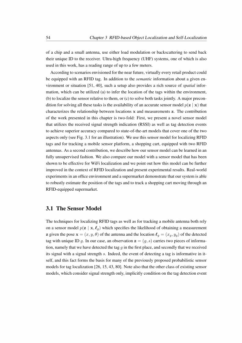
54 Chapter 3 RFID-based Object Localization and Self-Localization
of a chip and a small antenna, use either load modulation or backscattering to send backtheir unique ID to the receiver. Ultra-high frequency (UHF) systems, one of which is alsoused in this work, has a reading range of up to a few meters.
According to scenarios envisioned for the near future, virtually every retail product couldbe equipped with an RFID tag. In addition to the semantic information about a given en-vironment or situation [51, 40], such a setup also provides a rich source of spatial infor-mation, which can be utilized (a) to infer the location of the tags within the environment,(b) to localize the sensor relative to them, or (c) to solve both tasks jointly. A major precon-dition for solving all these tasks is the availability of an accurate sensor model p(z | x) thatcharacterizes the relationship between locations x and measurements z. The contributionof the work presented in this chapter is two-fold: First, we present a novel sensor modelthat utilizes the received signal strength indication (RSSI) as well as tag detection eventsto achieve superior accuracy compared to state-of-the-art models that cover one of the twoaspects only (see Fig. 3.1 for an illustration). We use this sensor model for localizing RFIDtags and for tracking a mobile sensor platform, a shopping cart, equipped with two RFIDantennas. As a second contribution, we describe how our sensor model can be learned in anfully unsupervised fashion. We also compare our model with a sensor model that has beenshown to be effective for WiFi localization and we point out how this model can be furtherimproved in the context of RFID localization and present experimental results. Real-worldexperiments in an office environment and a supermarket demonstrate that our system is ableto robustly estimate the position of the tags and to track a shopping cart moving through anRFID-equipped supermarket.
3.1 The Sensor Model
The techniques for localizing RFID tags as well as for tracking a mobile antenna both relyon a sensor model p(z | x, `g) which specifies the likelihood of obtaining a measurementz given the pose x = (x, y, θ) of the antenna and the location `g = (xg, yg) of the detectedtag with unique ID g. In our case, an observation z = (g, s) carries two pieces of informa-tion, namely that we have detected the tag g in the first place, and secondly that we receivedits signal with a signal strength s. Indeed, the event of detecting a tag is informative in it-self, and this fact forms the basis for many of the previously proposed probabilistic sensormodels for tag localization [26, 15, 43, 80]. Note also that the other class of existing sensormodels, which consider signal strength only, implicitly condition on the tag detection event

3.1 The Sensor Model 55
−2 −1 0 1 2 3 4
−1
0
1
[m]
[m]
5
6
7
8
(a) Mean of the logarithmic signal strength.
−2 −1 0 1 2 3 4
−1
0
1
[m]
[m]
0
0.5
1
1.5
2
(b) Standard deviation of the logarithmic signal strength.
−2 −1 0 1 2 3 4
−1
0
1
[m]
[m]
0
0.1
0.2
0.3
(c) Tag detection probability.
Figure 3.1: The proposed sensor model combines information about the expected received signal strength, (a)and (b), and about the probability of detecting a tag (c).
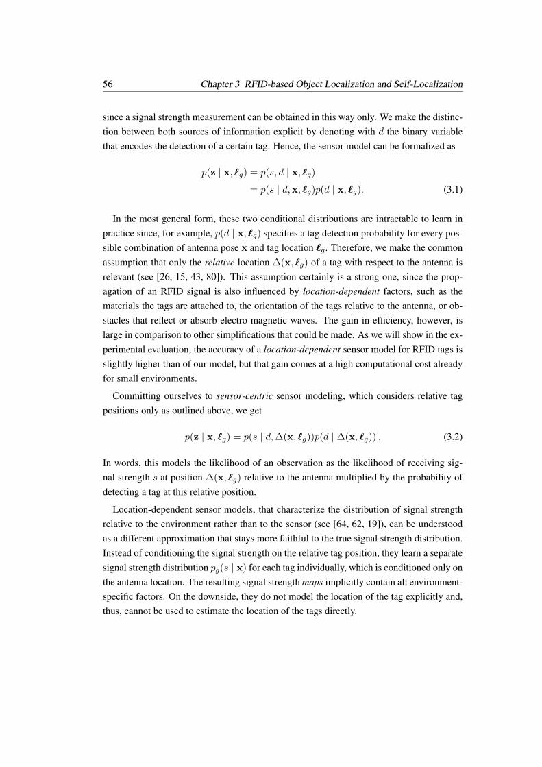
56 Chapter 3 RFID-based Object Localization and Self-Localization
since a signal strength measurement can be obtained in this way only. We make the distinc-tion between both sources of information explicit by denoting with d the binary variablethat encodes the detection of a certain tag. Hence, the sensor model can be formalized as
p(z | x, `g) = p(s, d | x, `g)
= p(s | d,x, `g)p(d | x, `g). (3.1)
In the most general form, these two conditional distributions are intractable to learn inpractice since, for example, p(d | x, `g) specifies a tag detection probability for every pos-sible combination of antenna pose x and tag location `g. Therefore, we make the commonassumption that only the relative location ∆(x, `g) of a tag with respect to the antenna isrelevant (see [26, 15, 43, 80]). This assumption certainly is a strong one, since the prop-agation of an RFID signal is also influenced by location-dependent factors, such as thematerials the tags are attached to, the orientation of the tags relative to the antenna, or ob-stacles that reflect or absorb electro magnetic waves. The gain in efficiency, however, islarge in comparison to other simplifications that could be made. As we will show in the ex-perimental evaluation, the accuracy of a location-dependent sensor model for RFID tags isslightly higher than of our model, but that gain comes at a high computational cost alreadyfor small environments.
Committing ourselves to sensor-centric sensor modeling, which considers relative tagpositions only as outlined above, we get
p(z | x, `g) = p(s | d,∆(x, `g))p(d | ∆(x, `g)) . (3.2)
In words, this models the likelihood of an observation as the likelihood of receiving sig-nal strength s at position ∆(x, `g) relative to the antenna multiplied by the probability ofdetecting a tag at this relative position.
Location-dependent sensor models, that characterize the distribution of signal strengthrelative to the environment rather than to the sensor (see [64, 62, 19]), can be understoodas a different approximation that stays more faithful to the true signal strength distribution.Instead of conditioning the signal strength on the relative tag position, they learn a separatesignal strength distribution pg(s | x) for each tag individually, which is conditioned only onthe antenna location. The resulting signal strength maps implicitly contain all environment-specific factors. On the downside, they do not model the location of the tag explicitly and,thus, cannot be used to estimate the location of the tags directly.
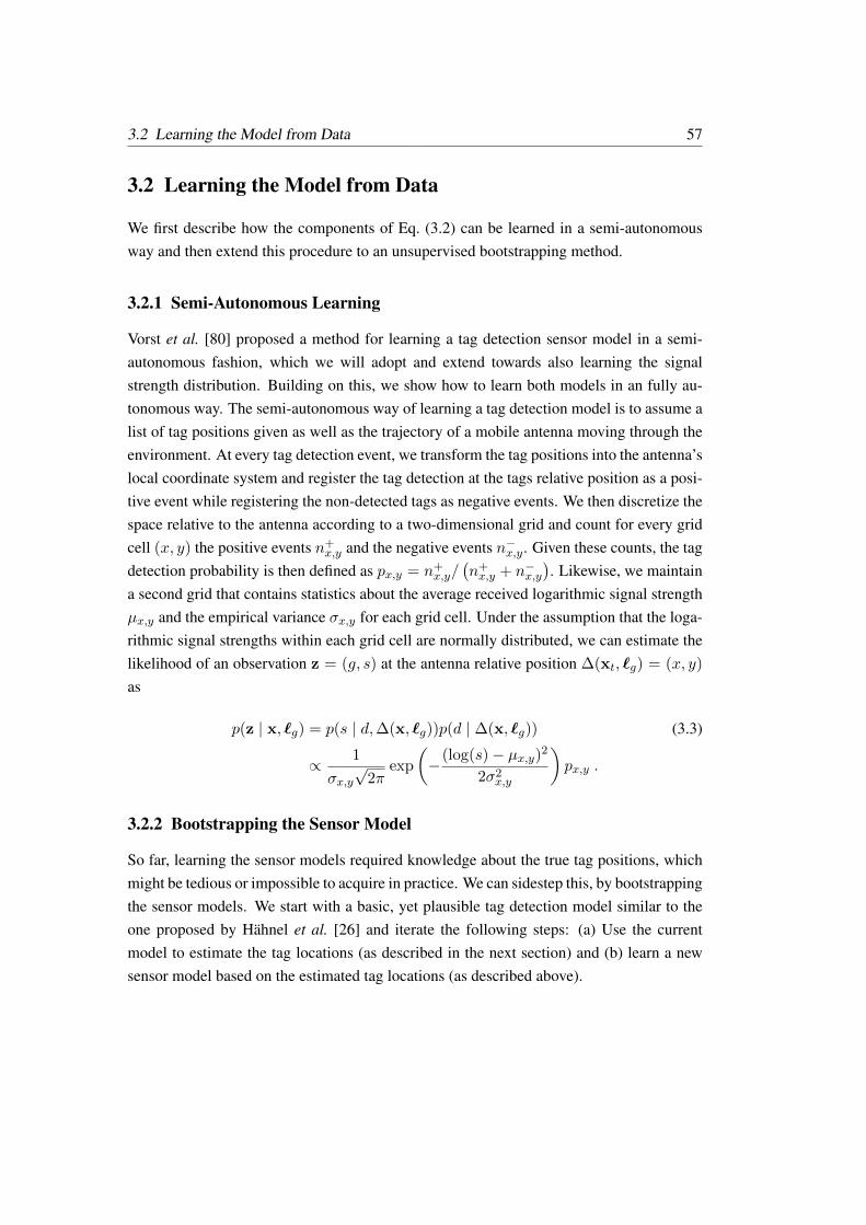
3.2 Learning the Model from Data 57
3.2 Learning the Model from Data
We first describe how the components of Eq. (3.2) can be learned in a semi-autonomousway and then extend this procedure to an unsupervised bootstrapping method.
3.2.1 Semi-Autonomous Learning
Vorst et al. [80] proposed a method for learning a tag detection sensor model in a semi-autonomous fashion, which we will adopt and extend towards also learning the signalstrength distribution. Building on this, we show how to learn both models in an fully au-tonomous way. The semi-autonomous way of learning a tag detection model is to assume alist of tag positions given as well as the trajectory of a mobile antenna moving through theenvironment. At every tag detection event, we transform the tag positions into the antenna’slocal coordinate system and register the tag detection at the tags relative position as a posi-tive event while registering the non-detected tags as negative events. We then discretize thespace relative to the antenna according to a two-dimensional grid and count for every gridcell (x, y) the positive events n+
x,y and the negative events n−x,y. Given these counts, the tagdetection probability is then defined as px,y = n+
x,y/(n+x,y + n−x,y
). Likewise, we maintain
a second grid that contains statistics about the average received logarithmic signal strengthµx,y and the empirical variance σx,y for each grid cell. Under the assumption that the loga-rithmic signal strengths within each grid cell are normally distributed, we can estimate thelikelihood of an observation z = (g, s) at the antenna relative position ∆(xt, `g) = (x, y)
as
p(z | x, `g) = p(s | d,∆(x, `g))p(d | ∆(x, `g)) (3.3)
∝ 1
σx,y√
2πexp
(−(log(s)− µx,y)2
2σ2x,y
)px,y .
3.2.2 Bootstrapping the Sensor Model
So far, learning the sensor models required knowledge about the true tag positions, whichmight be tedious or impossible to acquire in practice. We can sidestep this, by bootstrappingthe sensor models. We start with a basic, yet plausible tag detection model similar to theone proposed by Hähnel et al. [26] and iterate the following steps: (a) Use the currentmodel to estimate the tag locations (as described in the next section) and (b) learn a newsensor model based on the estimated tag locations (as described above).
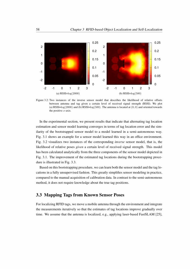
58 Chapter 3 RFID-based Object Localization and Self-Localization
0
0.05
0.1
0.15
0.2
0.25
-2 -1 0 1 2 3
-2
-1
0
1
2
(a) RSSI=log(2000)
0
0.05
0.1
0.15
0.2
0.25
-2 -1 0 1 2 3
-2
-1
0
1
2
(b) RSSI=log(500)
Figure 3.2: Two instances of the inverse sensor model that describes the likelihood of relative offsetsbetween antenna and tag given a certain level of received signal strength (RSSI). We plot(a) RSSI=log(2000) and (b) RSSI=log(500). The antenna is located at (0, 0) and oriented towardsthe positive x-axis.
In the experimental section, we present results that indicate that alternating tag locationestimation and sensor model learning converges in terms of tag location error and the sim-ilarity of the bootstrapped sensor model to a model learned in a semi-autonomous way.Fig. 3.1 shows an example for a sensor model learned this way in an office environment.Fig. 3.2 visualizes two instances of the corresponding inverse sensor model, that is, thelikelihood of relative poses given a certain level of received signal strength. This modelhas been calculated analytically from the three components of the sensor model depicted inFig. 3.1. The improvement of the estimated tag locations during the bootstrapping proce-dure is illustrated in Fig. 3.3.
Based on this bootstrapping procedure, we can learn both the sensor model and the tag lo-cations in a fully unsupervised fashion. This greatly simplifies sensor modeling in practice,compared to the manual acquisition of calibration data. In contrast to the semi-autonomousmethod, it does not require knowledge about the true tag positions.
3.3 Mapping Tags from Known Sensor Poses
For localizing RFID tags, we move a mobile antenna through the environment and integratethe measurements iteratively so that the estimates of tag locations improve gradually overtime. We assume that the antenna is localized, e.g., applying laser-based FastSLAM [25],
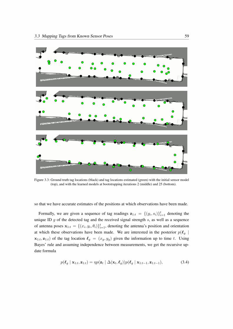
3.3 Mapping Tags from Known Sensor Poses 59
Figure 3.3: Ground truth tag locations (black) and tag locations estimated (green) with the initial sensor model(top), and with the learned models at bootstrapping iterations 2 (middle) and 25 (bottom).
so that we have accurate estimates of the positions at which observations have been made.
Formally, we are given a sequence of tag readings z1:t = (gi, si)ti=1 denoting theunique ID g of the detected tag and the received signal strength s, as well as a sequenceof antenna poses x1:t = (xi, yi, θi)ti=1, denoting the antenna’s position and orientationat which these observations have been made. We are interested in the posterior p(`g |x1:t, z1:t) of the tag location `g = (xg, yg) given the information up to time t. UsingBayes’ rule and assuming independence between measurements, we get the recursive up-date formula
p(`g | x1:t, z1:t) = ηp(zt | ∆(xt, `g))p(`g | x1:t−1, z1:t−1), (3.4)
60 Chapter 3 RFID-based Object Localization and Self-Localization
where p(zt | ∆(xt, `g)) is the sensor model described in the previous section and η is anormalization factor (see also [26]).
To estimate this posterior sequentially as new data arrives, we apply a particle filter foreach tag and use its unique ID g for data association. Each filter is initialized with a uniformparticle distribution (w(i)
g , `(i)g )i, where w(i)
g denotes the weight of a particle and `(i)g its
location. The initial particle distribution is bounded by the maximum reading range ofthe antenna and centered around the antenna’s position during the first encounter of thetag [visualized in Fig. 3.4 (a)]. We resample whenever the so-called number of effectiveparticles
neff =1∑
i(w(i))2
(3.5)
falls below a threshold κ, which we set to half the number of particles of the filter. In theresampling step, we follow Liu and West [42], and disturb the individual particle locationsby resampling them from a normal distribution with the following parametrization
`(i)g ∼ N (µLW,ΣLW) (3.6)
µLW = a`(i)g + (1− a)µg (3.7)
ΣLW = h2Σg (3.8)
Here, µg and Σg are the mean and covariance matrix of the particle set of tag g and the twoparameters a and h2 are defined as
a =3γ − 1
2γ(3.9)
h2 = 1− a2 (3.10)
and only depend on a discount factor γ, which we set to 0.95. This procedure causesthe particle-based estimates of the tag locations to converge to the true locations even forcrudely initialized estimates within a few filter iterations, as can be seen in Fig. 3.4.
3.4 Localizing a Mobile Agent
Given that we know the locations of the RFID tags, we can use the very same sensormodel to track a mobile agent equipped with an RFID antenna. We apply Monte CarloLocalization (MCL) [11], which utilizes a particle filter to maintain the posterior over the

3.4 Localizing a Mobile Agent 61
(a)I
nitia
lfilte
rsta
te.
(b)A
fter
seco
ndfil
teru
pdat
e.
(c)A
fter
5th
filte
rupd
ate.
(d)A
fter
30th
filte
rupd
ate.
Figu
re3.
4:L
ocal
izin
gR
FID
tags
inan
offic
eco
rrid
or:
The
gree
nci
rcle
indi
cate
sth
ees
timat
edta
glo
catio
nan
dth
ebl
ack
circ
leth
epo
seof
the
shop
ping
cart
.
62 Chapter 3 RFID-based Object Localization and Self-Localization
agent’s location
bel(xt+1) ∝ p(zt+1 | ∆(xt+1, `g))
∫xt
p(xt+1 | xt) bel(xt) dxt . (3.11)
While the sensor model p(z | ∆(x, `g)) remains the same, the crucial part here is themotion model p(xt+1 | xt), from which we sample the next particle distribution. As we aretracking a shopping cart, which does not provide odometry information, we used a velocitybased motion model that tries to capture the typical motion patterns of people pushing thecart. For this, each particle s(i) is constrained in a seven-dimensional space
s(i) = (x,v,m) = (x, y, θ, vx, vy, vθ,m) , (3.12)
that consists of the current pose x = (x, y, θ) of the cart, its velocity v = (vx, vy, vθ), anda motion statem. The velocity is parameterized by the translational velocity vx in directionof the cart, a lateral drift velocity vy, and a rotational velocity vθ. The discrete motion statem can assume one of the following seven values: standing, moving forwards (backwards),turning left forwards (backwards), or turning right forwards (backwards).
The transition from one particle state s(i)t to the state s
(i)t+1 at the next point in time is
modeled as follows: first, we sample a new motion statemt+1 according to a state transitionprobability p(mt+1 | mt). If the motion state changed, we sample new velocities vt+1 fromthree motion state-specific normal distributions
vx ∼ N (µm,x, σ2m,x) (3.13)
vy ∼ N (µm,y, σ2m,y) (3.14)
vθ ∼ N (µm,θ, σ2m,θ) (3.15)
that capture the velocity distributions of the particular motion state. If the sampled motionstate is the same as in the time step before, we do not sample new velocities, but ratherkeep the velocities of the previous point in time. Once the new velocities are determined,we deterministically compute the new pose of a particle based on the velocities and the timepassed during one filter update step. As during tag localization, we resample whenever thenumber of effective particles is less than half of the particle set size. To account for physicalconstraints imposed by walls and other obstacles, we set the weight of a particle close tozero, whenever it enters an occupancy grid cell that is likely to be occupied. The transitionprobabilities p(mt+1 | mt) and the parameters of the velocity distributions (µm,x, σ2
m,x,
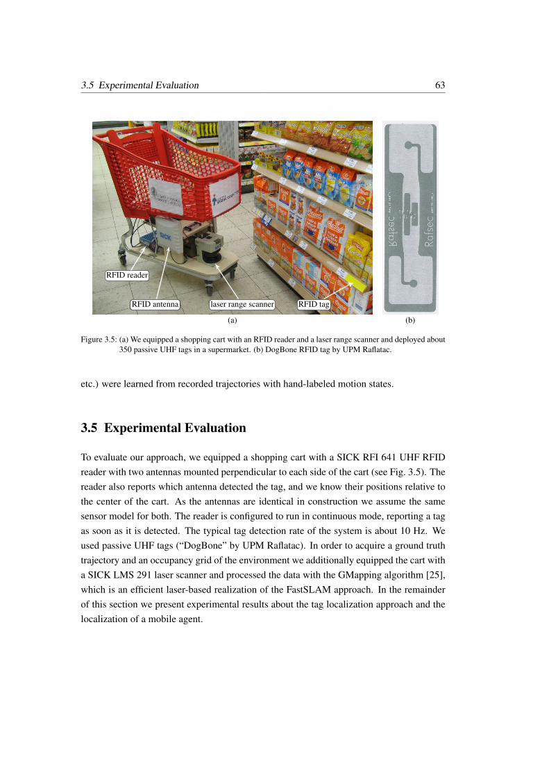
3.5 Experimental Evaluation 63
RFID tag
RFID reader
RFID antenna laser range scanner
(a) (b)
Figure 3.5: (a) We equipped a shopping cart with an RFID reader and a laser range scanner and deployed about350 passive UHF tags in a supermarket. (b) DogBone RFID tag by UPM Raflatac.
etc.) were learned from recorded trajectories with hand-labeled motion states.
3.5 Experimental Evaluation
To evaluate our approach, we equipped a shopping cart with a SICK RFI 641 UHF RFIDreader with two antennas mounted perpendicular to each side of the cart (see Fig. 3.5). Thereader also reports which antenna detected the tag, and we know their positions relative tothe center of the cart. As the antennas are identical in construction we assume the samesensor model for both. The reader is configured to run in continuous mode, reporting a tagas soon as it is detected. The typical tag detection rate of the system is about 10 Hz. Weused passive UHF tags (“DogBone” by UPM Raflatac). In order to acquire a ground truthtrajectory and an occupancy grid of the environment we additionally equipped the cart witha SICK LMS 291 laser scanner and processed the data with the GMapping algorithm [25],which is an efficient laser-based realization of the FastSLAM approach. In the remainderof this section we present experimental results about the tag localization approach and thelocalization of a mobile agent.

64 Chapter 3 RFID-based Object Localization and Self-Localization
3.5.1 Localizing the RFID Tags
We distributed 28 RFID tags in an office corridor as depicted by the black circles in Fig. 3.3on page 59. Neighboring tags had an average distance of about two meters. We knewthe true locations of the tags and therefore could evaluate the accuracy of tag localizationquantitatively. We bootstrapped the sensor model by moving the shopping cart up and downthe corridor several times – performing 360 turns at several locations. This took about 4minutes and resulted in roughly 4 100 tag detections. Fig. 3.6 (a) shows the evolution ofthe average error of the estimated tag locations after each iteration of the bootstrappingprocess. As can be seen, the error converges to a final value of about 29 cm. We alsogive the estimation results for the signal strength-based model alone (red line) and the tagdetection-based model alone (blue line) evaluated on the same trajectory. Our proposedcombined sensor model (black line) is significantly better than either the signal strength-based model or the tag detection-based one alone.
If we learn the sensor model semi-autonomously based on the true tag locations, weachieve a localization accuracy of about 27 cm instead of 29 cm. This indicates, that thebootstrapping process yields a sensor model that is comparable to a semi-autonomouslylearned sensor model. This was also confirmed by visually comparing the individual com-ponents of the two models. To confirm this finding quantitatively, we calculated the aver-age symmetric Kullback-Leibler divergence between all grid cells of the two models aftereach bootstrapping iteration. The results illustrated in Figs. 3.6 (b) and (c) show that thebootstrapping process also converges in terms of model similarity to a semi-autonomouslylearned model.
3.5.2 Localizing a Mobile Agent
We distributed about 350 tags along the shelves in a supermarket at an average distance ofapproximately one meter. Then we bootstrapped the sensor models and the tag positionsby using data from six log files, which we collected by moving the shopping cart throughthe environment. The log files contained 34 200 tag detections and lasted about 74 minutesin total. We used the localization technique described above and defined as the localizationresult the trajectory of the most likely particle. An example of an estimated trajectory andits corresponding ground truth trajectory is depicted in Fig. 3.7.
To evaluate the accuracy of the localization technique quantitatively, we localized theagent on seven different log files which lasted 24 minutes in total and contained 13 400 tagdetections. We repeatedly localized the cart for each log file ten times and averaged the

3.5 Experimental Evaluation 65
2 4 6 8 10 12 14 16 18 20 22 240.2
0.4
0.6
0.8
bootstrapping iteration
tag
loca
tion
erro
r[m
]signal strength modeltag detection model
combined model
(a) Average tag localization error.
2 4 6 8 10 12 14 16 18 20 22 24
0.2
0.4
0.6
0.8
bootstrapping iteration
Kul
lbac
k-L
eibl
erdi
verg
ence KLD signal strength models
(b) Divergence of the signal strength models.
2 4 6 8 10 12 14 16 18 20 22 24
2
4
6
8
·10−2
bootstrapping iteration
Kul
lbac
k-L
eibl
erdi
verg
ence KLD tag detection models
(c) Divergence of the tag detection models.
Figure 3.6: The bootstrapping process: (a) The process converges in terms of the average tag location error.The error bars depict the 2σ confidence interval. (b) and (c) show that the bootstrapping procedurealso converges in terms of sensor model similarity to a semi-autonomously learned model.
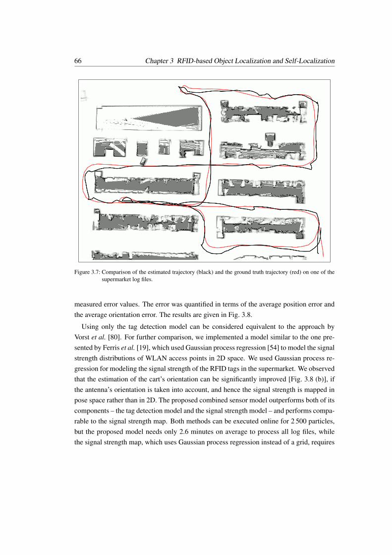
66 Chapter 3 RFID-based Object Localization and Self-Localization
Figure 3.7: Comparison of the estimated trajectory (black) and the ground truth trajectory (red) on one of thesupermarket log files.
measured error values. The error was quantified in terms of the average position error andthe average orientation error. The results are given in Fig. 3.8.
Using only the tag detection model can be considered equivalent to the approach byVorst et al. [80]. For further comparison, we implemented a model similar to the one pre-sented by Ferris et al. [19], which used Gaussian process regression [54] to model the signalstrength distributions of WLAN access points in 2D space. We used Gaussian process re-gression for modeling the signal strength of the RFID tags in the supermarket. We observedthat the estimation of the cart’s orientation can be significantly improved [Fig. 3.8 (b)], ifthe antenna’s orientation is taken into account, and hence the signal strength is mapped inpose space rather than in 2D. The proposed combined sensor model outperforms both of itscomponents – the tag detection model and the signal strength model – and performs compa-rable to the signal strength map. Both methods can be executed online for 2 500 particles,but the proposed model needs only 2.6 minutes on average to process all log files, whilethe signal strength map, which uses Gaussian process regression instead of a grid, requires

3.5 Experimental Evaluation 67
250 500 1,000 2,5000.2
0.4
0.6
0.8
1
1.2
1.4
1.6
1.8
2
number of particles
aver
age
posi
tion
erro
r[m
] signal strength map (pose)signal strength map (point)
signal strength modeltag detection model
proposed combined model
2,5000.3
0.35
0.4
0.45
0.5
0.55
0.6
0.65
(a) Average position error.
250 500 1,000 2,5000.2
0.25
0.3
0.35
0.4
0.45
0.5
0.55
0.6
0.65
number of particles
aver
age
orie
ntat
ion
erro
r[ra
d]
2,5000.15
0.2
0.25
0.3
0.35
0.4
0.45
(b) Average orientation error.
250 500 1,000 2,5000
2.5
5
7.5
10
12.5
number of particles
runt
ime
[min
]
(c) Runtime.
Figure 3.8: Evaluation of several sensor models for RFID-based localization: the proposed combined model,and its two components alone. For comparison, we show the results of a signal strength map,similar to the model by Ferris et al. [19], mapping the signal strength either in pose space (“pose”)or in 2D (“point”).
68 Chapter 3 RFID-based Object Localization and Self-Localization
13.4 minutes, as can be seen in Fig. 3.8 (c).
In both tasks – localization and mapping – the signal strength model alone was con-sistently less accurate than the tag detection model. This is an unexpected finding, sincethe received signal strength should intuitively be more informative than a simple detec-tion event. Close inspection of the recorded data reveals, however, that the relationshipbetween signal-strength and sensor location is more noisy than it is the case for tag detec-tions. Thus, the particle filter as a sophisticated way of integrating information over time,is able to recover the (real-valued) pose information accurately from the stream of (binary)tag detection events.
3.6 Future Work
There are several directions for future work. Our results showed that considering signalstrength information along with tag detection events lead to an improved sensor centricmodel. Therefore, it would be interesting to see if the accuracy of signal strength mapscould be improved in just the same way by combining them with “tag detection maps”.Another direction would be to extend the model to a 3D sensor model. Moreover, theassumption made that the tag map remains static could be alleviated – a technique for map-ping “nomadic” tags (static tags which change locations from time to time) was presentedin [43].
3.7 Related Work
There is a variety of approaches to RFID-based localization, which can be characterizedby the type of sensor information used as well as by the general approach to modelingthis information. Some of the earlier systems only provided information about the ID ofthe detected tag while later systems also provide information about the received signalstrength. Hence, some localization techniques utilize sensor models that are based onlyon tag detection events [26, 37, 60, 15, 43]. For some RFID readers that do not provideRSSI (signal strength) directly, this information can be emulated by means of differentattenuation levels or power levels of the antenna [48, 1, 36]. Sensor models for localizingtags are usually designed to be sensor centric [26, 15, 43, 1, 12]. A different design, thatcan be used for localizing a mobile robot, is to lay out the sensor model relative to theenvironment [60, 64, 62, 19].

3.8 Conclusions 69
Hähnel et al. [26] utilized a piecewise constant tag detection sensor model to first localizethe tags and then use the tag map to localize a mobile antenna. Schneegans et al. [60]compared histograms of tag detections with previously recorded histograms at differentlocations. Kleiner et al. [37] used a combination of pedestrian odometry and tag detectionsto perform graph-based RFID SLAM in a large outdoor environment. Kanda et al. [36]deployed RFID readers in a science museum and tracked people with attached RFID tags.Vorst et al. [80] showed how to learn a tag detection sensor model in a semi-autonomousfashion. Some approaches in the context of WiFi localization model the expected signalstrength at different locations by using a discrete grid [64], or Gaussian process regression[62, 19].
Several approaches have addressed exclusively the tag localization problem. Ni et al. [48]compared the (emulated) signal strengths of tags at unknown locations with signal strengthsreceived from reference tags at known locations. Alippi et al. [1] used several rotating an-tennas. Ehrenberg et al. [15] used an HF RFID system to localize books on a shelf. Liu etal. [43] used a tag detection model that is able to estimate the 3D position of the tag.Deyle et al. [13] introduced the concept of RSSI images, which are acquired by panningand tilting an RFID antenna attached to a robot while recording the RSSI measurements.
In contrast to the above-mentioned approaches, we model both phenomena – tag detec-tion events as well as signal strength. The increased accuracy of the model allows us toaddress (a) localization of a mobile sensor relative to given tag locations and (b) mappingof tag locations when these are unknown. Furthermore, we showed how to simultane-ously learn the sensor model and estimate the position of the RFID tags in an unsupervisedfashion. We presented real-world experiments in an office environment as well as in asupermarket environment and compared our approach with state-of-the-art methods.
3.8 Conclusions
In this chapter, we presented a novel combined sensor model that utilizes both (a) the re-ceived signal strength and (b) tag detections of RFID systems for robot localization andmapping of tags. We also presented a technique to learn such a model in an unsupervisedway. This greatly simplifies the task of sensor modeling in practice compared to the man-ual acquisition of calibration data. For comparison, we implemented a sensor model thathas been shown to be effective for WiFi localization. We furthermore described how thismodel can be improved in the context of RFID localization. As our experiments in several

70 Chapter 3 RFID-based Object Localization and Self-Localization
real-world settings showed, our approach achieves the computational efficiency of existingsensor-centric models and an accuracy of a state-of-the-art approach that learns a location-dependent model for each tag.
Our proposed technique enables a mobile robot to localize and identify objects. Theresulting object map consists of a list of object locations and object IDs. We now moveon to the question how robots can take advantage of such object maps and how to leverageknowledge about usual object arrangements to more efficiently carry out their tasks. Inparticular, we are interested in finding an object in an unknown environment that has to beexplored while searching for the object. As a motivating application scenario, we considerthe search for a product in unknown supermarket. This will be the topic of the next chapter.
CHAPTER 4
Searching for Objects
We consider the problem of efficiently finding an object with a mobilerobot in an initially unknown, structured environment. The overallgoal is to allow the robot to improve upon a standard explorationtechnique by utilizing background knowledge from previously seen,similarly structured environments. We present two conceptually differentapproaches. Whereas the first method is a reactive search techniquethat decides where to search next only based on local informationabout the objects in the robot’s vicinity, the second algorithm is a moreglobal and inference-based approach that explicitly reasons about thelocation of the target object given all observations made so far. Whilethe model underlying the first approach can be learned from data ofoptimal search paths, we learn the model of the second method fromobject arrangements of example environments. Our application scenariois the search for a product in a supermarket. We present simulationand real-world experiments in which we compare our strategies toalternative methods and also to the performance of humans.
Consider the situation where you want to find a product in a supermarket where youhave never been to before. Certainly, you will not just wander around randomly throughthe market nor will you systematically visit each so far unvisited aisle in the market untilyou find the product. Your search will rather be guided by the current observations andthe expectations you have about how objects in supermarkets are usually arranged. Overtime, you might even have developed some heuristics that proved to be useful for quickly
72 Chapter 4 Searching for Objects
finding a certain product, like “if you want to find yogurt, follow the aisle with the coolingshelves.”
The search for a product in an unknown supermarket is a problem that everyone is famil-iar with and it therefore is an illustrative instance of the kind of search problems we want totackle with the techniques presented in this chapter. Even for humans [75] this task is notan easy one and we will also compare our search techniques to the performance of humanparticipants that took part in a field study conducted in a real supermarket [35]. However,the supermarket is just an example scenario. Searching for objects or places in offices ordomestic environments is conceptually similar. All we assume is that the environment isstructured and the object arrangements exhibit some spatial dependencies such that a gen-eralization to an unknown yet similarly structured environment is possible. We regard thisas a rather weak assumption that holds for a huge variety of man-made environments. Wethus strive for a general way to model, learn, and utilize background knowledge such thata mobile robot is able to find an object more efficiently than it would have been possiblewithout such domain-specific knowledge. For this, we present and evaluate two approachesand provide alternative views on the search problem.
The first approach is a reactive search technique that only depends on local informationabout the objects in the robot’s vicinity when deciding where to search next. This approachemphasizes the sequential nature of the search process, which is a sequential decision mak-ing process. Being in a certain state we must choose among a set of available actions. Inthis setting, background knowledge can be encoded as a state-to-action mapping, a policy,that tells us what to do in a certain situation. In the supermarket scenario, a state includesthe currently observed objects in direction of the different aisles and the available actionscorrespond to the aisle we may choose to visit next. To learn this state-to-action mapping,we draw on ideas from imitation learning [3]. In particular, we want to imitate a simu-lated robot that exhibits an optimal search behavior by approaching the target object on theshortest path. In each visited state of a demonstrated example path, the robot takes a certainaction and discards the other available actions in this state. Thereby, it provides positiveand negative examples of state-action pairs to be taken or not, respectively. These examplescan be used to learn a classifier for state-action pairs, which yields a classifier-based policyrepresentation [55]. This might either be a multi-class classifier that directly outputs the ac-tion to be taken in a given state, or it might be a binary classifier that labels each availableaction in a state as promising or non-promising (if there is a tie, we may choose randomlyamong the promising actions). The latter has been empirically shown [55] to yield poli-cies that perform better than the ones that are represented by multi-class classifiers. We
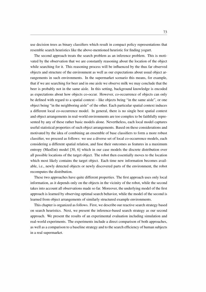
73
use decision trees as binary classifiers which result in compact policy representations thatresemble search heuristics like the above-mentioned heuristic for finding yogurt.
The second approach treats the search problem as an inference problem. This is moti-vated by the observation that we are constantly reasoning about the location of the objectwhile searching for it. This reasoning process will be influenced by the thus far observedobjects and structure of the environment as well as our expectations about usual object ar-rangements in such environments. In the supermarket scenario this means, for example,that if we are searching for beer and in one aisle we observe milk we may conclude that thebeer is probably not in the same aisle. In this setting, background knowledge is encodedas expectations about how objects co-occur. However, co-occurrence of objects can onlybe defined with regard to a spatial context – like objects being “in the same aisle”, or oneobject being “in the neighboring aisle” of the other. Each particular spatial context inducesa different local co-occurrence model. In general, there is no single best spatial contextand object arrangements in real-world environments are too complex to be faithfully repre-sented by any of these rather basic models alone. Nevertheless, each local model capturesuseful statistical properties of such object arrangements. Based on these considerations andmotivated by the idea of combining an ensemble of base classifiers to form a more robustclassifier, we proceed as follows: we use a diverse set of local co-occurrence models, eachconsidering a different spatial relation, and fuse their outcomes as features in a maximumentropy (MaxEnt) model [30, 6] which in our case models the discrete distribution overall possible locations of the target object. The robot then essentially moves to the locationwhich most likely contains the target object. Each time new information becomes avail-able, i.e., newly detected objects or newly discovered parts of the environment, the robotrecomputes the distribution.
These two approaches have quite different properties. The first approach uses only localinformation, as it depends only on the objects in the vicinity of the robot, while the secondtakes into account all observations made so far. Moreover, the underlying model of the firstapproach is learned by observing optimal search behavior, while the model of the second islearned from object arrangements of similarly structured example environments.
This chapter is organized as follows. First, we describe our reactive search strategy basedon search heuristics. Next, we present the inference-based search strategy as our secondapproach. We present the results of an experimental evaluation including simulation andreal-world experiments. The experiments include a direct comparison of both approaches,as well as a comparison to a baseline strategy and to the search efficiency of human subjectsin a real supermarket.
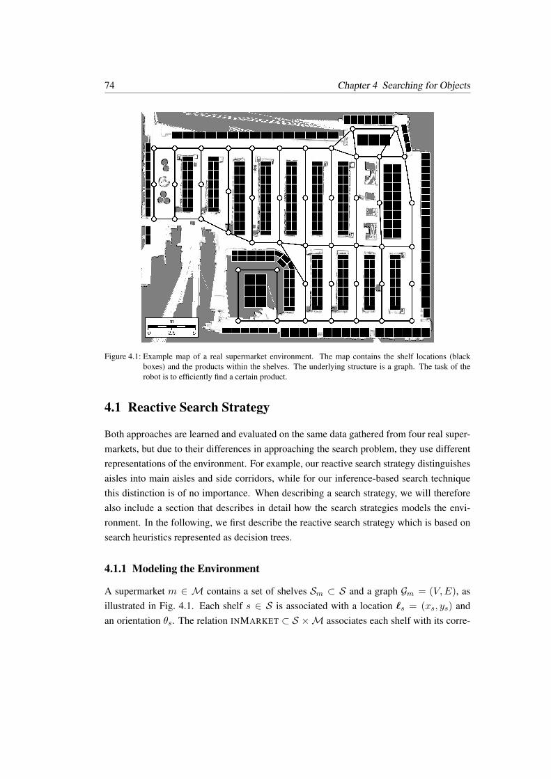
74 Chapter 4 Searching for Objects
Figure 4.1: Example map of a real supermarket environment. The map contains the shelf locations (blackboxes) and the products within the shelves. The underlying structure is a graph. The task of therobot is to efficiently find a certain product.
4.1 Reactive Search Strategy
Both approaches are learned and evaluated on the same data gathered from four real super-markets, but due to their differences in approaching the search problem, they use differentrepresentations of the environment. For example, our reactive search strategy distinguishesaisles into main aisles and side corridors, while for our inference-based search techniquethis distinction is of no importance. When describing a search strategy, we will thereforealso include a section that describes in detail how the search strategies models the envi-ronment. In the following, we first describe the reactive search strategy which is based onsearch heuristics represented as decision trees.
4.1.1 Modeling the Environment
A supermarket m ∈ M contains a set of shelves Sm ⊂ S and a graph Gm = (V,E), asillustrated in Fig. 4.1. Each shelf s ∈ S is associated with a location `s = (xs, ys) andan orientation θs. The relation INMARKET ⊂ S ×M associates each shelf with its corre-
4.1 Reactive Search Strategy 75
Figure 4.2: Three example situations for illustrating the short range visibility. Whereas gray shelves are visible,white shelves are not visible. The location of the robot is indicated by the black node and itsorientation is indicated by the arrow.
sponding market. Furthermore, we define a set of shelf types T = NORMAL, COOLING,FREEZER, COUNTER, GROCERY and each shelf is associated with exactly one type asdefined by the relation TYPE ⊂ S × T . Each shelf contains at least one product and thesame product might be placed in several shelves, as defined by the relation INSHELF ⊂P × S. The relation CATEGOF ⊂ P × C, associates each product with a product category.
For the experiments, we used a set of 196 products at the granularity of small categorieslike “sugar”, “pizza”, “apples”, “tea”, etc. We furthermore used 20 product categories witha coarser granularity like “breakfast”, “dairy products”, “vegetables & fruits”, etc.
The nodes V of a graph Gm = (V,E) model the decision points in the supermarket andthe directed edges define the reachability between decision points. While the reachabilitycould have been modeled with undirected edges, the visibility of the shelves also dependson the current node (the robot’s current location) and therefore is defined over directededges. We use two variants of a visibility relation that defines the shelves that are visiblewhen looking into the direction of a certain edge. The first one is a long range variantSHELFVISL ⊂ E × S and the second is a short range variant SHELFVISS ⊆ SHELFVISL.This is motivated by the fact that, although certain information, like the type of a shelf, canbe determined reliably over long distances, some information can only be determined whenone is in close vicinity to a shelf, like for example the products contained within a shelf.Three example situations illustrating the short range visibility are depicted in Fig. 4.2. On
76 Chapter 4 Searching for Objects
the basis of the two visibility relations we define several other visibility relations, like thevisible products
PRODVIS = (e, p) | SHELFVISS(e, s), INSHELF(p, s), (4.1)
and the visible product categories
CATEGVIS = (e, c) | PRODVIS(e, p), CATEGOF(p, c). (4.2)
The visibility of shelf types is modeled in such a way that we can distinguish whether theshelf type is seen in the direct vicinity, or being observed at a further distance:
TYPEVISS = (e, t) | SHELFVISS(e, s), TYPE(s, t) (4.3)
TYPEVISL = (e, t) | SHELFVISL(e, s), TYPE(s, t). (4.4)
The reactive search strategy utilizes the information associated with each edge to decidewhich edge to follow. In the next section we describe how we learn such a strategy fromdata by observing optimal search paths.
4.1.2 Learning Search Heuristics
We are interested in learning a reactive search strategy that depends only on local informa-tion in order to find a certain target product. We therefore classify the outgoing edges ofthe current node by a decision tree into promising and non-promising directions based onthe information associated with each edge. For learning such a decision tree, we first needto define appropriate edge attributes and then gather training data by generating optimalsearch paths in a training set of supermarkets. To evaluate the strategy, we apply it to apreviously unseen market.
4.1.2.1 Defining Edge Attributes
One obvious piece of information, by which the search should be guided, is which productsand product categories are visible at a certain edge. If we are searching for coffee and anaisle contains tea, or in general breakfast products, then this edge is certainly a promisingcandidate. But the decision should also be influenced by additional factors. If we knowthat an edge has been visited already, we can reject it in order to avoid loops. Also the typeof an edge might be of interest, such as if an edge belongs to an aisle that follows a wall
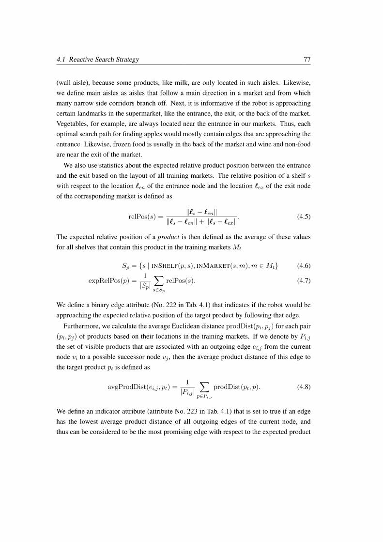
4.1 Reactive Search Strategy 77
(wall aisle), because some products, like milk, are only located in such aisles. Likewise,we define main aisles as aisles that follow a main direction in a market and from whichmany narrow side corridors branch off. Next, it is informative if the robot is approachingcertain landmarks in the supermarket, like the entrance, the exit, or the back of the market.Vegetables, for example, are always located near the entrance in our markets. Thus, eachoptimal search path for finding apples would mostly contain edges that are approaching theentrance. Likewise, frozen food is usually in the back of the market and wine and non-foodare near the exit of the market.
We also use statistics about the expected relative product position between the entranceand the exit based on the layout of all training markets. The relative position of a shelf swith respect to the location `en of the entrance node and the location `ex of the exit nodeof the corresponding market is defined as
relPos(s) =‖`s − `en‖
‖`s − `en‖+ ‖`s − `ex‖. (4.5)
The expected relative position of a product is then defined as the average of these valuesfor all shelves that contain this product in the training markets Mt
Sp = s | INSHELF(p, s), INMARKET(s,m),m ∈Mt (4.6)
expRelPos(p) =1
|Sp|∑s∈Sp
relPos(s). (4.7)
We define a binary edge attribute (No. 222 in Tab. 4.1) that indicates if the robot would beapproaching the expected relative position of the target product by following that edge.
Furthermore, we calculate the average Euclidean distance prodDist(pi, pj) for each pair(pi, pj) of products based on their locations in the training markets. If we denote by Pi,jthe set of visible products that are associated with an outgoing edge ei,j from the currentnode vi to a possible successor node vj , then the average product distance of this edge tothe target product pt is defined as
avgProdDist(ei,j , pt) =1
|Pi,j |∑p∈Pi,j
prodDist(pt, p). (4.8)
We define an indicator attribute (attribute No. 223 in Tab. 4.1) that is set to true if an edgehas the lowest average product distance of all outgoing edges of the current node, andthus can be considered to be the most promising edge with respect to the expected product

78 Chapter 4 Searching for Objects
Table 4.1: The attributes that are used to characterize an edge. All attributes are binary. In the experimentalevaluation we test different combinations of subsets (a–d) of these attributes.
Subset Att. No. Description
a 1 Edge already visiteda 2–197 Product pi ∈ P visiblea 198–217 Product of category ci ∈ C visiblea 218 Shelf of type NORMAL visible (short range)a 219 Shelf of type COOLING visible (short range)a 220 Shelf of type FREEZER visible (short range)a 221 Shelf of type COUNTER visible (short range)b 222 Leads to expected relative positionb 223 Has smallest avg. Euclidean distance to productb 224 Has smallest avg. path distance to productc 225 Current node belongs to a main aislec 226 Next node belongs to a main aislec 227 Next node belongs to a wall aislec 228–230 Leads to the entrance, exit, or back of the marketd 231 Shelf of type COOLING visible (long range)d 232 Shelf of type FREEZER visible (long range)d 233 Shelf of type GROCERY visible (long range)
distances. Likewise, we define an attribute that uses the path distance on the graph betweenproducts instead of the Euclidean distance (attribute No. 224). As it is not easy to decidebeforehand whether the path distance or the Euclidean distance is a more reliable indicatorfor product distances we use both attributes and let the learning algorithm decide whichone to use during the induction of the tree. A complete list of all attributes can be seen inTab. 4.1.
4.1.2.2 Generating Training Data
We use a fixed set of 15 target products. These are the same products that human partici-pants had to find in a field study conducted in the very same supermarket in which we willevaluate our strategy. We learn a separate decision tree for each of these 15 target products.
We determine for each node in a training supermarket the shortest path to a given targetproduct. Each node of an optimal path corresponds to a local decision for taking a certainoutgoing edge (the one that leads to the next node of the optimal path) and for rejecting allother outgoing edges of that node. In this way, each optimal search path contributes a set ofpositive and negative examples of edges to be taken or not, respectively. Fig. 4.3 illustratesthe basic idea. The positive and negative examples of all paths for all starting positions in

4.1 Reactive Search Strategy 79
Start
Goal
(a) Shortest path between starting location and goal location.
(b) Local decision at one of the nodes along the path.
Figure 4.3: (a) For generating training data, we compute the shortest path from every possible starting locationin the market for a given goal location of a target product. One such path is depicted above. (b) Eachnode of an optimal path corresponds to a local decision for taking a certain outgoing edge (blacksolid arrow) and for rejecting all other outgoing edges of that node (gray dashed arrows). In thisway, each optimal search path contributes a set of positive and negative examples of edges to betaken or not, respectively.
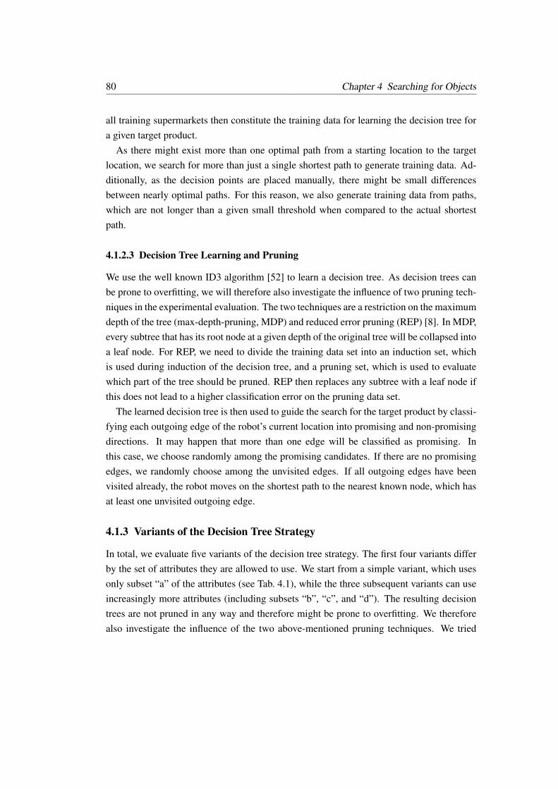
80 Chapter 4 Searching for Objects
all training supermarkets then constitute the training data for learning the decision tree fora given target product.
As there might exist more than one optimal path from a starting location to the targetlocation, we search for more than just a single shortest path to generate training data. Ad-ditionally, as the decision points are placed manually, there might be small differencesbetween nearly optimal paths. For this reason, we also generate training data from paths,which are not longer than a given small threshold when compared to the actual shortestpath.
4.1.2.3 Decision Tree Learning and Pruning
We use the well known ID3 algorithm [52] to learn a decision tree. As decision trees canbe prone to overfitting, we will therefore also investigate the influence of two pruning tech-niques in the experimental evaluation. The two techniques are a restriction on the maximumdepth of the tree (max-depth-pruning, MDP) and reduced error pruning (REP) [8]. In MDP,every subtree that has its root node at a given depth of the original tree will be collapsed intoa leaf node. For REP, we need to divide the training data set into an induction set, whichis used during induction of the decision tree, and a pruning set, which is used to evaluatewhich part of the tree should be pruned. REP then replaces any subtree with a leaf node ifthis does not lead to a higher classification error on the pruning data set.
The learned decision tree is then used to guide the search for the target product by classi-fying each outgoing edge of the robot’s current location into promising and non-promisingdirections. It may happen that more than one edge will be classified as promising. Inthis case, we choose randomly among the promising candidates. If there are no promisingedges, we randomly choose among the unvisited edges. If all outgoing edges have beenvisited already, the robot moves on the shortest path to the nearest known node, which hasat least one unvisited outgoing edge.
4.1.3 Variants of the Decision Tree Strategy
In total, we evaluate five variants of the decision tree strategy. The first four variants differby the set of attributes they are allowed to use. We start from a simple variant, which usesonly subset “a” of the attributes (see Tab. 4.1), while the three subsequent variants can useincreasingly more attributes (including subsets “b”, “c”, and “d”). The resulting decisiontrees are not pruned in any way and therefore might be prone to overfitting. We thereforealso investigate the influence of the two above-mentioned pruning techniques. We tried

4.2 Inference-based Search Strategy 81
several alternatives by restricting the maximum depth of the trees to different levels (MDP)or by applying reduced error pruning (REP), or a combination of both to any of the fourattribute subset variants. We found the best variant to be a combination of both pruningtechniques applied to a tree that uses the full set of attributes. We first applied MDP usinga maximum depth of four and then additionally applied REP. To do so, the training data setwas split into an induction set (75% of the data) and a pruning set (25% of the data). Twoexamples of learned and pruned decision trees can be seen in Fig. 4.4 on the next page.
4.2 Inference-based Search Strategy
In this section, we describe our second approach, the inference-based search strategy. Wefocus on the problem of how background knowledge about usual arrangements of objectscan be utilized to more efficiently find an object. The basic idea of this approach is to splitthe action selection problem during the search process into two parts. First, we compute abelief over possible locations of the target object based on the information about the objectsseen so far and the structure of the environment. Second, we utilize the belief to select thenext action, e.g., the next position the robot moves to.
The representation for encoding the background knowledge about object arrangementsis motivated by the fact that structured indoor environments exhibit meaningful spatial re-lations between locations that influence the distribution of the objects. For example, onemight link two locations by relations like “the same room”, or “the same floor”. Further-more, we think that in order to be able to generalize from previously seen environments tonew environments it is advantageous to represent objects by a list of attributes, instead ofthinking of them as atomic entities. For example, even if you have never seen an avocado ina supermarket, it will be useful to know that it is a fruit and it is therefore probably locatedsomewhere where you will see other objects of the category “fruit”.
The definition of the object attributes and the types of spatial relations are the onlydomain-specific parts of this second approach. It is therefore also applicable to other appli-cation scenarios, like finding an object in an office environment or a domestic environmentas long as it is provided with the corresponding relevant attributes and spatial relations.
4.2.1 Modeling the Evironment
We collected real-world data from four supermarkets, including the market layout and theproducts in each shelf. We defined a set of 181 products at the granularity of small cate-
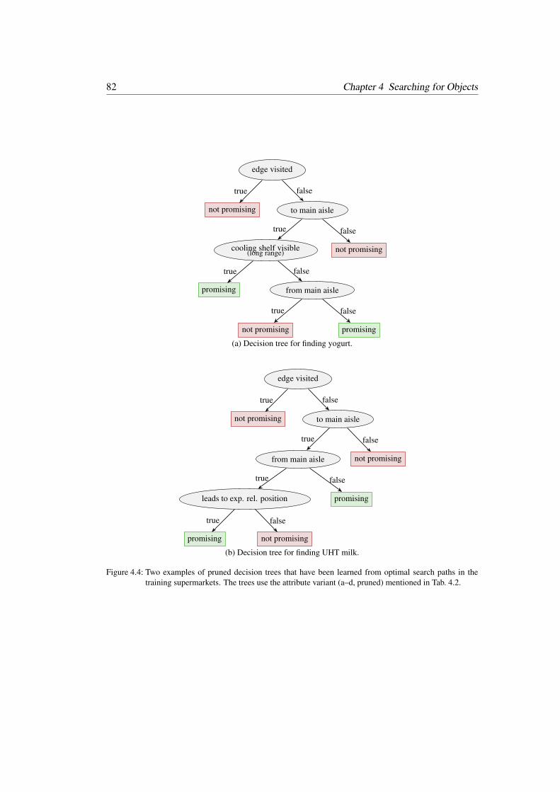
82 Chapter 4 Searching for Objects
edge visited
not promising
true
to main aisle
cooling shelf visible(long range)
promising
true
from main aisle
not promising
true
promising
false
false
true
not promising
false
false
(a) Decision tree for finding yogurt.
edge visited
not promising
true
to main aisle
from main aisle
leads to exp. rel. position
promising
true
not promising
false
true
promising
false
true
not promising
false
false
(b) Decision tree for finding UHT milk.
Figure 4.4: Two examples of pruned decision trees that have been learned from optimal search paths in thetraining supermarkets. The trees use the attribute variant (a–d, pruned) mentioned in Tab. 4.2.

4.2 Inference-based Search Strategy 83
gories like pizza, apple, shampoo, etc. Additionally, each product is associated with one of20 product categories with a coarser granularity like breakfast, dairy products, vegetables& fruits, etc. Further attributes of products are the binary “edible” attribute, as well as theattribute “shelf type”, that denotes in which shelf type the product is usually found in. Thiscan be normal, cooling, freezer, or counter. We consider the basic structural elements ofa supermarket to be approximately one meter wide shelves, which are depicted as boxesin Fig. 4.5 and Fig. 4.6 on the next pages. Moreover, we will define a “shelf wall unit”to be made up of adjacent shelves standing side by side, such as the red region marked inFig. 4.8 on page 89. Each shelf contains at least one product and a product might be placedin several shelves.
Additionally, the representation of a market contains a graph that constrains the motionof the robot. Each shelf is associated with an access node which is defined to be its nearestgraph node. The search process ends, if the robot is located at the access node of a shelfthat contains the target product. The robot does not know the environment beforehand butrather has to explore it during the search. The structure of the environment – shelves andgraph nodes – can be observed from any distance within the market, as long as they are inthe line of sight. In contrast, the products of a shelf can only be detected within a distanceof two meters. These visibility constraints are motivated by taking into account the sensorlimitations of a real robot. The graph could be extracted from a grid map by constructinga Voronoi graph and the shelf locations could be identified by assuming that each wall orobstacle in the map is a shelf. For the actual detection of the objects, we assume that therobot is equipped with an RFID sensor and the products are equipped with RFID tags. Ina supermarket environment the robot would then be able to reliably locate a product whenit is about two or three meters away. However, the model described here is not restrictedto these sensor modalities, we only require the robot to be able to sense the structure of theenvironment and to detect and localize objects. The next section will introduce our modelfor inferring the location of the target object that the robot is searching for.
4.2.2 A Model for Inferring Object Locations
We have a set O = onNon=1 of detectable objects and each object is described by a setA = AiNii=1 of attributes, each with a finite domainD(Ai) of possible values ai ∈ D(Ai).We wish to infer the location of a query object oq ∈ O, which we assume to be at one ofseveral possible locations X = xlNll=1. We furthermore have a set of spatial relationsR = rjNrr=1, that relate locations of detected objects to locations x ∈ X , like “same
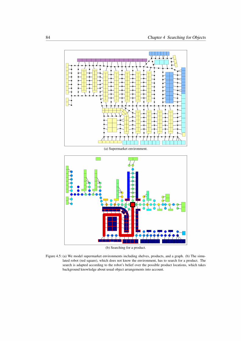
84 Chapter 4 Searching for Objects
(a) Supermarket environment.
(b) Searching for a product.
Figure 4.5: (a) We model supermarket environments including shelves, products, and a graph. (b) The simu-lated robot (red square), which does not know the environment, has to search for a product. Thesearch is adapted according to the robot’s belief over the possible product locations, which takesbackground knowledge about usual object arrangements into account.
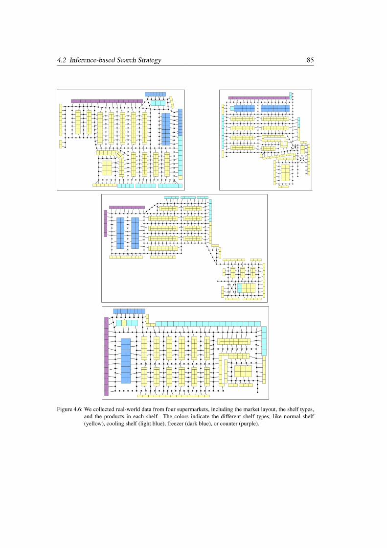
4.2 Inference-based Search Strategy 85
Figure 4.6: We collected real-world data from four supermarkets, including the market layout, the shelf types,and the products in each shelf. The colors indicate the different shelf types, like normal shelf(yellow), cooling shelf (light blue), freezer (dark blue), or counter (purple).
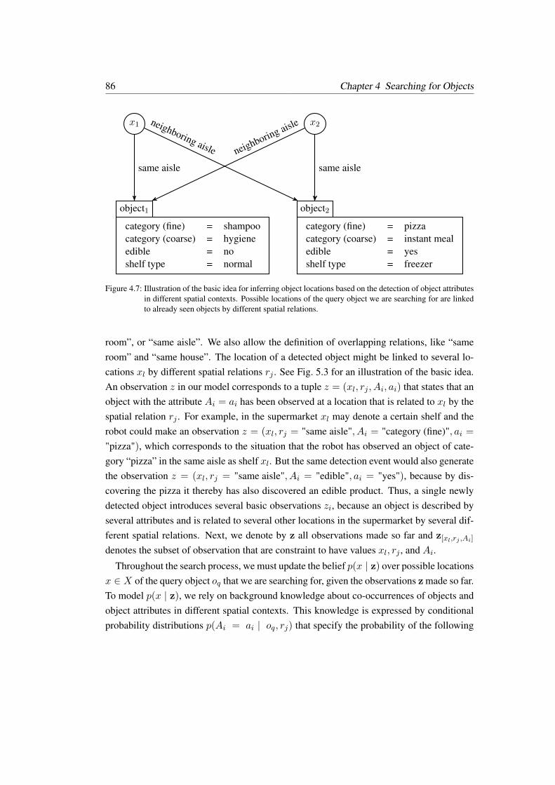
86 Chapter 4 Searching for Objects
x1 x2
object1 object2
category (fine) = shampoocategory (coarse) = hygieneedible = noshelf type = normal
category (fine) = pizzacategory (coarse) = instant mealedible = yesshelf type = freezer
same aisle
neighboring aisle neighboring aisle
same aisle
Figure 4.7: Illustration of the basic idea for inferring object locations based on the detection of object attributesin different spatial contexts. Possible locations of the query object we are searching for are linkedto already seen objects by different spatial relations.
room”, or “same aisle”. We also allow the definition of overlapping relations, like “sameroom” and “same house”. The location of a detected object might be linked to several lo-cations xl by different spatial relations rj . See Fig. 5.3 for an illustration of the basic idea.An observation z in our model corresponds to a tuple z = (xl, rj , Ai, ai) that states that anobject with the attribute Ai = ai has been observed at a location that is related to xl by thespatial relation rj . For example, in the supermarket xl may denote a certain shelf and therobot could make an observation z = (xl, rj = "same aisle", Ai = "category (fine)", ai =
"pizza"), which corresponds to the situation that the robot has observed an object of cate-gory “pizza” in the same aisle as shelf xl. But the same detection event would also generatethe observation z = (xl, rj = "same aisle", Ai = "edible", ai = "yes"), because by dis-covering the pizza it thereby has also discovered an edible product. Thus, a single newlydetected object introduces several basic observations zi, because an object is described byseveral attributes and is related to several other locations in the supermarket by several dif-ferent spatial relations. Next, we denote by z all observations made so far and z[xl,rj ,Ai]
denotes the subset of observation that are constraint to have values xl, rj , and Ai.
Throughout the search process, we must update the belief p(x | z) over possible locationsx ∈ X of the query object oq that we are searching for, given the observations z made so far.To model p(x | z), we rely on background knowledge about co-occurrences of objects andobject attributes in different spatial contexts. This knowledge is expressed by conditionalprobability distributions p(Ai = ai | oq, rj) that specify the probability of the following
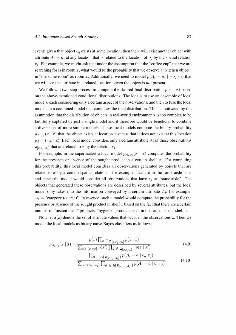
4.2 Inference-based Search Strategy 87
event: given that object oq exists at some location, then there will exist another object withattribute Ai = ai at any location that is related to the location of oq by the spatial relationrj . For example, we might ask that under the assumption that the “coffee cup” that we aresearching for is in room x, what would be the probability that we observe a “kitchen object”in “the same room” as room x. Additionally, we need to model p(Ai = ai | ¬oq, rj) thatwe will see the attribute in a related location, given the object is not present.
We follow a two step process to compute the desired final distribution p(x | z) basedon the above-mentioned conditional distributions. The idea is to use an ensemble of localmodels, each considering only a certain aspect of the observations, and then to fuse the localmodels in a combined model that computes the final distribution. This is motivated by theassumption that the distribution of objects in real-world environments is too complex to befaithfully captured by just a single model and it therefore would be beneficial to combinea diverse set of more simple models. These local models compute the binary probabilitypAi,rj (x | z) that the object exists at location x versus that it does not exist at this locationpAi,rj (¬x | z). Each local model considers only a certain attributeAi of those observationsz[x,rj ,Ai] that are related to x by the relation rj .
For example, in the supermarket a local model pAi,rj (x | z) computes the probabilityfor the presence or absence of the sought product in a certain shelf x. For computingthis probability, this local model considers all observations generated by objects that arerelated to x by a certain spatial relation – for example, that are in the same aisle as xand hence the model would consider all observations that have rj = "same aisle". Theobjects that generated these observations are described by several attributes, but the localmodel only takes into the information conveyed by a certain attribute Ai, for example,Ai = "category (coarse)". In essence, such a model would compute the probability for thepresence or absence of the sought product in shelf x based on the fact that there are a certainnumber of “instant meal” products, “hygiene” products, etc., in the same aisle as shelf x.
Now let a(z) denote the set of attribute values that occur in the observations z. Then wemodel the local models as binary naive Bayes classifiers as follows:
pAi,rj (x | z) =p(x)
∏z ∈ z[x,rj ,Ai]
p(z | x)∑x′∈x,¬x p(x
′)∏z ∈ z[x,rj ,Ai]
p(z | x′)(4.9)
=
∏a ∈ a(z[x,rj ,Ai])
p(Ai = a | oq, rj)∑o′∈oq ,¬oq
∏a ∈ a(z[x,rj ,Ai])
p(Ai = a | o′, rj). (4.10)
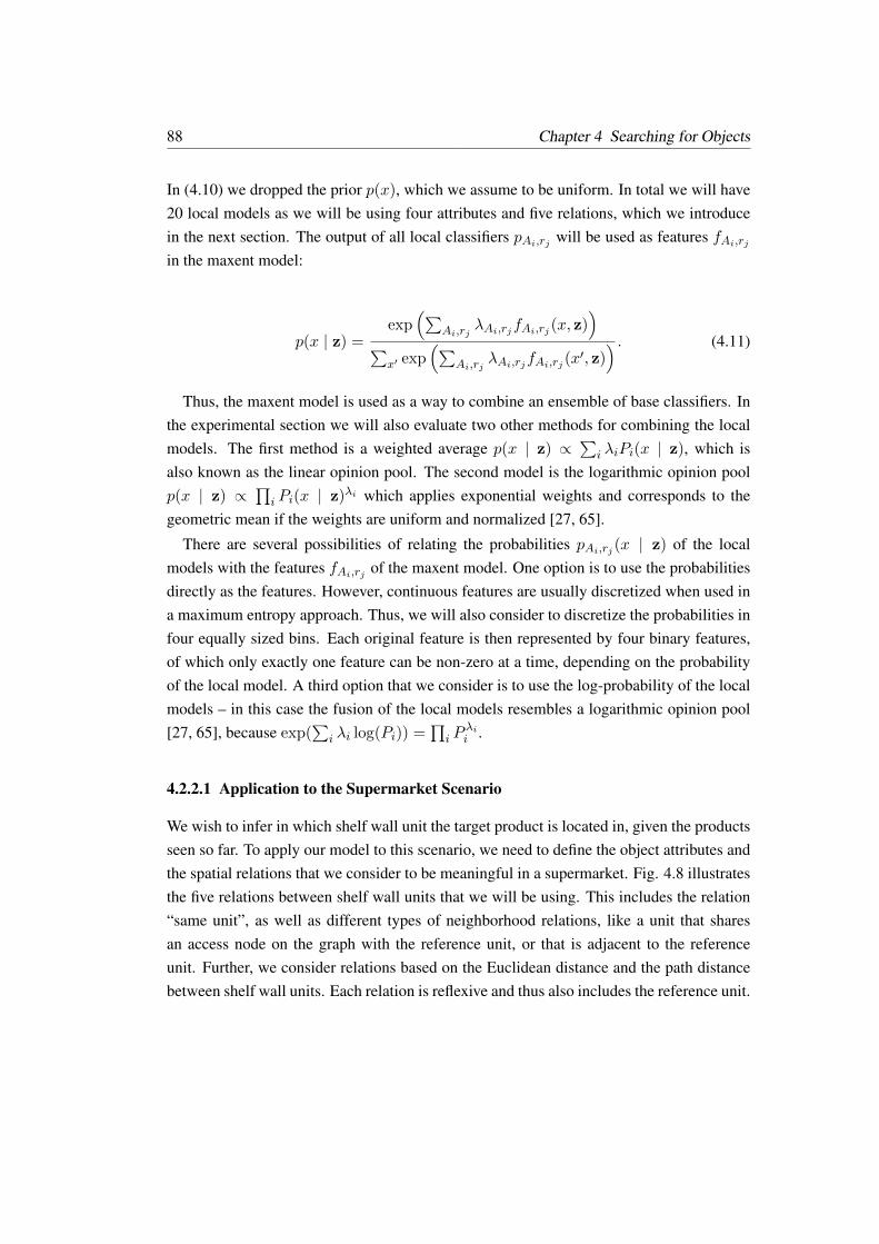
88 Chapter 4 Searching for Objects
In (4.10) we dropped the prior p(x), which we assume to be uniform. In total we will have20 local models as we will be using four attributes and five relations, which we introducein the next section. The output of all local classifiers pAi,rj will be used as features fAi,rjin the maxent model:
p(x | z) =exp
(∑Ai,rj
λAi,rjfAi,rj (x, z))
∑x′ exp
(∑Ai,rj
λAi,rjfAi,rj (x′, z)
) . (4.11)
Thus, the maxent model is used as a way to combine an ensemble of base classifiers. Inthe experimental section we will also evaluate two other methods for combining the localmodels. The first method is a weighted average p(x | z) ∝
∑i λiPi(x | z), which is
also known as the linear opinion pool. The second model is the logarithmic opinion poolp(x | z) ∝
∏i Pi(x | z)λi which applies exponential weights and corresponds to the
geometric mean if the weights are uniform and normalized [27, 65].
There are several possibilities of relating the probabilities pAi,rj (x | z) of the localmodels with the features fAi,rj of the maxent model. One option is to use the probabilitiesdirectly as the features. However, continuous features are usually discretized when used ina maximum entropy approach. Thus, we will also consider to discretize the probabilities infour equally sized bins. Each original feature is then represented by four binary features,of which only exactly one feature can be non-zero at a time, depending on the probabilityof the local model. A third option that we consider is to use the log-probability of the localmodels – in this case the fusion of the local models resembles a logarithmic opinion pool[27, 65], because exp(
∑i λi log(Pi)) =
∏i P
λii .
4.2.2.1 Application to the Supermarket Scenario
We wish to infer in which shelf wall unit the target product is located in, given the productsseen so far. To apply our model to this scenario, we need to define the object attributes andthe spatial relations that we consider to be meaningful in a supermarket. Fig. 4.8 illustratesthe five relations between shelf wall units that we will be using. This includes the relation“same unit”, as well as different types of neighborhood relations, like a unit that sharesan access node on the graph with the reference unit, or that is adjacent to the referenceunit. Further, we consider relations based on the Euclidean distance and the path distancebetween shelf wall units. Each relation is reflexive and thus also includes the reference unit.

4.2 Inference-based Search Strategy 89
(a) Same unit. (b) Adjacent unit.
(c) Shared access node unit. (d) Short Euclidean distance unit.
(e) Short path distance unit.
Figure 4.8: We use five relations between shelf wall units. The reference unit is marked in red (dark gray) andthe related units in blue (light gray). The relations are: (a) The same shelf wall unit. (b) Unitsadjacent to the reference unit. (c) Units sharing an access node with the reference unit. (d) Unitswithin an Euclidean distance of four meters, or (e) within a path distance of four meters. Allrelations are reflexive and thus also include the reference unit.

90 Chapter 4 Searching for Objects
The attributes we are using are the ones that already have been depicted in Fig. 5.3 on page112. These are: fine category, coarse category, shelf type, and edible. Some examples ofthe fine categories (pizza, shampoo, etc.) and coarse categories (instant meal, hygiene, etc.)that we are using were given in Section 4.2.1 on page 81.
To learn the feature weights we set up the training data in the following way: first weestimate the conditional probabilities p(Ai = ai | oq, rj) based on the data of three su-permarkets by simply counting the basic events. The local models are then used in themaximum entropy model as features to predict the locations of objects in the remainingfourth supermarket. This is done for all four supermarket combinations and for all 141products, that are available in all markets. Thus, in total we have 4 × 141 training exam-ples. We train a single set of parameters. The learned weights therefore reflect the generalimportance of each local model when being used to predict a new situation – independentof a specific product or market. During the search process, we will only observe a smallfraction of all products in the market. The model is therefore trained on markets in whichonly some of the shelves contain products. It takes less than two minutes to train the modelon a standard PC and each inference during the search takes less than 10 ms.
4.2.3 Selecting a Target Location
Once a belief over the possible location of the target object is computed, the robot needs todecide which action to take next. However, we are facing two problems, when planning apath based on the current belief. First, ideally we should take future observations into ac-count, which will change the belief and the subsequent steps. Second, even if we ignore fornow that new evidence will change this belief, the problem of planning an optimal searchpath that minimizes the expected search path length with respect to a given distribution isstill NP-hard [77, 5]. We will thus settle for a heuristic approach.
If the robot greedily plans the shortest path to the node with the highest detection prob-ability, it will exhibit undesirable oscillating behavior when there is more than one modein the belief. We therefore use a strategy that computes a utility U(v) for each node vthat trades off the (relative) detection probability p(v) at this node with the (relative) pathdistance d(v) needed to reach it:
U(v) = αp(v)
maxv′ p(v′)− (1− α)
d(v)
maxv′ d(v′). (4.12)
Selecting a target location by trading off the benefits and costs in a weighted sum has been

4.3 Experimental Evaluation 91
m
0 5 10
detection probability
0 > 0.1
node utility
-0.6 > 0.6
simulated robot
shampoo
Figure 4.9: Example run using the maxent search technique with log-probability features. The position of therobot is marked by the big red square and the path taken is marked by the red line.
previously used in autonomous exploration [44, 67]. By adjusting the parameter α ∈ [0, 1]
we can alter the search behavior. We tried several parameters in 0.1 increments and foundα = 0.4 to result in the shortest paths. The robot moves on the shortest path to the unvisitednode with the highest utility until new observations are made and the belief and the nodeutilities have to be re-evaluated. In Fig. 4.9 we illustrate several stages of an example runin one of the supermarkets. This concludes the description of our second search strategyproposed in this chapter. The next section presents the results of several experiments toquantitatively evaluate both strategies.
4.3 Experimental Evaluation
The first experiment is aimed at comparing the performance of the different search strate-gies in comparison to the performance of humans searching in a real supermarket envi-
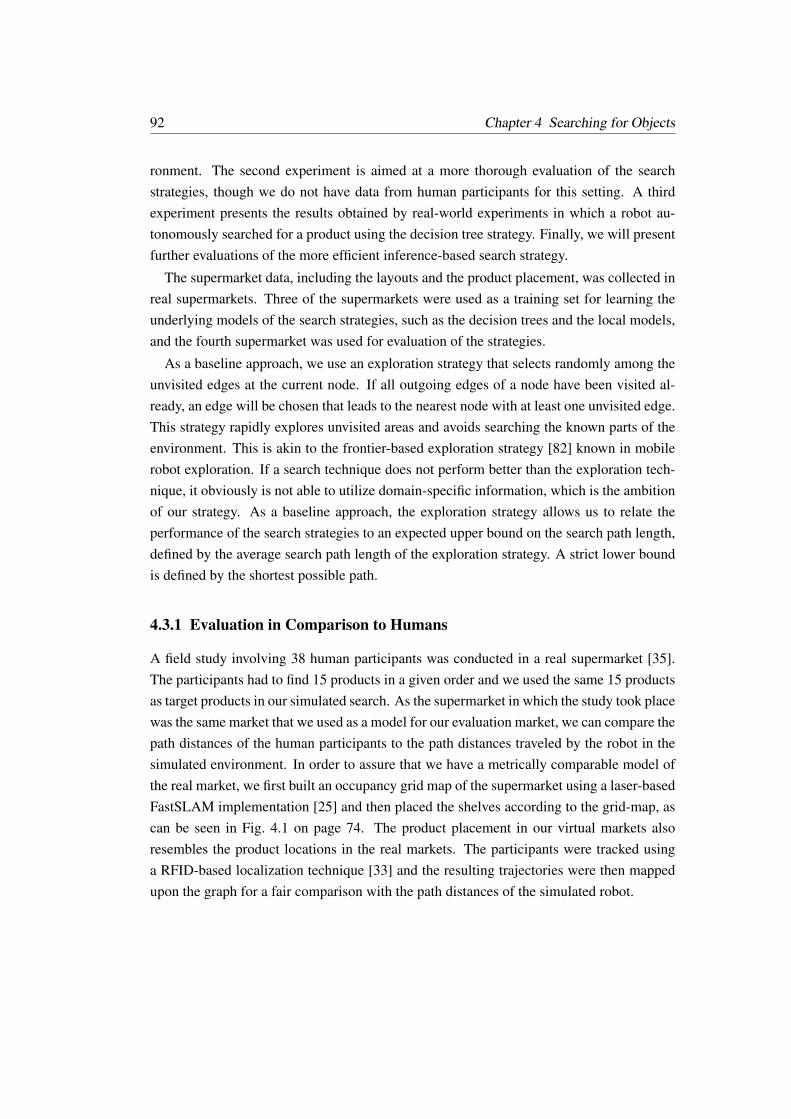
92 Chapter 4 Searching for Objects
ronment. The second experiment is aimed at a more thorough evaluation of the searchstrategies, though we do not have data from human participants for this setting. A thirdexperiment presents the results obtained by real-world experiments in which a robot au-tonomously searched for a product using the decision tree strategy. Finally, we will presentfurther evaluations of the more efficient inference-based search strategy.
The supermarket data, including the layouts and the product placement, was collected inreal supermarkets. Three of the supermarkets were used as a training set for learning theunderlying models of the search strategies, such as the decision trees and the local models,and the fourth supermarket was used for evaluation of the strategies.
As a baseline approach, we use an exploration strategy that selects randomly among theunvisited edges at the current node. If all outgoing edges of a node have been visited al-ready, an edge will be chosen that leads to the nearest node with at least one unvisited edge.This strategy rapidly explores unvisited areas and avoids searching the known parts of theenvironment. This is akin to the frontier-based exploration strategy [82] known in mobilerobot exploration. If a search technique does not perform better than the exploration tech-nique, it obviously is not able to utilize domain-specific information, which is the ambitionof our strategy. As a baseline approach, the exploration strategy allows us to relate theperformance of the search strategies to an expected upper bound on the search path length,defined by the average search path length of the exploration strategy. A strict lower boundis defined by the shortest possible path.
4.3.1 Evaluation in Comparison to Humans
A field study involving 38 human participants was conducted in a real supermarket [35].The participants had to find 15 products in a given order and we used the same 15 productsas target products in our simulated search. As the supermarket in which the study took placewas the same market that we used as a model for our evaluation market, we can compare thepath distances of the human participants to the path distances traveled by the robot in thesimulated environment. In order to assure that we have a metrically comparable model ofthe real market, we first built an occupancy grid map of the supermarket using a laser-basedFastSLAM implementation [25] and then placed the shelves according to the grid-map, ascan be seen in Fig. 4.1 on page 74. The product placement in our virtual markets alsoresembles the product locations in the real markets. The participants were tracked usinga RFID-based localization technique [33] and the resulting trajectories were then mappedupon the graph for a fair comparison with the path distances of the simulated robot.
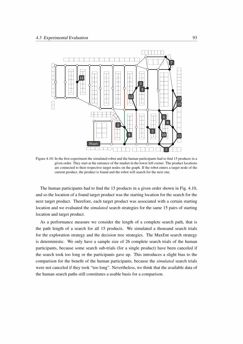
4.3 Experimental Evaluation 93
13
1
2
3
4
5
6
7
8
9 10 11
14
15
12
Start
Figure 4.10: In the first experiment the simulated robot and the human participants had to find 15 products in agiven order. They start at the entrance of the market in the lower left corner. The product locationsare connected to their respective target nodes on the graph. If the robot enters a target node of thecurrent product, the product is found and the robot will search for the next one.
The human participants had to find the 15 products in a given order shown in Fig. 4.10,and so the location of a found target product was the starting location for the search for thenext target product. Therefore, each target product was associated with a certain startinglocation and we evaluated the simulated search strategies for the same 15 pairs of startinglocation and target product.
As a performance measure we consider the length of a complete search path, that isthe path length of a search for all 15 products. We simulated a thousand search trialsfor the exploration strategy and the decision tree strategies. The MaxEnt search strategyis deterministic. We only have a sample size of 26 complete search trials of the humanparticipants, because some search sub-trials (for a single product) have been canceled ifthe search took too long or the participants gave up. This introduces a slight bias to thecomparison for the benefit of the human participants, because the simulated search trialswere not canceled if they took “too long”. Nevertheless, we think that the available data ofthe human search paths still constitutes a usable basis for a comparison.

94 Chapter 4 Searching for Objects
Table 4.2: Mean and standard deviation (SD) of the overall search path lengths for different search strategies.For further comparison we list the length of the optimal path and the path length ratio defined as theaverage path length of a strategy divided by the length of the optimal path.
StrategySearch Path Length
Ratio SamplesMean (km) SD (km)
Exploration 1.959 0.297 7.9 1000
Dec. Tree (a–d, pruned) 1.176 0.211 4.8 1000Dec. Tree (a) 1.609 0.263 6.5 1000Dec. Tree (a–b) 1.425 0.193 5.8 1000Dec. Tree (a–c) 1.620 0.257 6.6 1000Dec. Tree (a–d) 1.717 0.238 7.0 1000
MaxEnt (single run) 0.342 – 1.4 –MaxEnt (restarts) 0.911 – 3.7 –
Human Participants 0.565 0.110 2.3 26
Optimal Path 0.247 – 1.0 –
In Tab. 4.2 we present the mean and standard deviation of the search path lengths. Weperformed a one-tailed paired t-test1 for the sampled strategies and found all improvementsindicated by the means to be significant at the 0.01 level, except for the difference betweenthe decision trees with attribute combinations (a) and (a–c).
The exploration strategy yielded search paths that are on average 7.9 times longer thanthe optimal path. This can be improved to a ratio of 4.8 when the search was guided byour proposed strategy based on the pruned decision trees. If we used unpruned decisiontrees then the best ratio we achieved was 5.8. This seems to suggest that the unpruneddecision trees overfit the data of the three training supermarkets. The MaxEnt strategyachieved the best result with a ratio of 1.4. However, by using the MaxEnt strategy therobot built up a global map during the search that also included the locations of all productsseen so far. Thus, if a target product has been seen previously while searching for anotherproduct, the product could later be approached directly on the shortest path. As the otherstrategies lack the ability to memorize the global locations of previously seen products, wealso considered a modified version of the MaxEnt strategy (the “restart” version in Tab. 4.2)in which the map was cleared when a product has been found. Thus, when searching for thenext product on the list, the robot could not utilize information about the market stemming
1If the sample sizes differed, we used the sample size of the smaller sample. We also applied Welch’s t-test,which is applicable for unequal sample sizes and unequal variances, and got the same results regarding thestatistical significance at the 0.01 level.

4.3 Experimental Evaluation 95
from the search sub-trial for the previous product. This resulted in a ratio of 3.7, which isstill better than the decision tree strategy, though it now performs worse than the humanparticipants who achieved a ratio of 2.3. However, one might argue that humans certainlydo build up some kind of global map of the market during the search and thus are ableto utilize information from previous search sub-trials when searching for the next product.Clearly, this information is less accurate and more sketchy than the map utilized in the“single run” version of the MaxEnt strategy that memorizes the exact location of all seenproducts.
Though the proposed strategies did not achieve the same performance as humans, the re-sults clearly indicate that the utilization of background knowledge by our proposed strate-gies leads to significantly shorter search paths when compared to an uninformed searchstrategy. The exploration strategy performed significantly worse than our approaches, be-cause it is not able to take domain-specific background knowledge into account, which isthe advantage of our proposed techniques.
4.3.2 Evaluation with Varying Starting Locations
The setting presented in the previous section was restricted to a single starting location foreach target product. This was motivated by the desired comparison to the performance ofthe human participants, for which we had to replicate the conditions of the field study.
For a more thorough evaluation of the search strategies, we started the search for thetarget products from several different locations. We randomly chose 20 starting locationsin the market. These are depicted in Fig. 4.11 on the next page. Each of the 15 productsfrom the previous experiment had to be searched for from each starting location, yielding300 independent search trials per strategy. For the MaxEnt strategy, the map was clearedbetween the individual search trials. As in the previous experiment, we considered the totalsearch path length of all individual search trials as a performance measure for the searchstrategies. We repeated each experiment a thousand times and list the average total searchpath length and its standard deviation in Tab. 4.3 on the next page.
Beside the exploration strategy we evaluated the variant of our decision tree strategythat performed the best in the previous experiment. Though the improvement over theexploration strategy was now less pronounced than in the previous setting, it still yieldssignificantly2 shorter search paths, as can be seen in Tab. 4.3. The MaxEnt strategy yields
2We performed one-tailed paired t-tests with p < 0.01 for the sampled strategies. The result of the MaxEntstrategy also differs significantly (p < 0.01) from the results of the sampled strategies.

96 Chapter 4 Searching for Objects
Figure 4.11: For the second experiment we randomly chose 20 starting locations (filled nodes) for the searchtrials. The target locations of the products remain the same as in the previous experiment (seeFig. 4.10).
Table 4.3: Mean and standard deviation (SD) of the overall search path lengths for different search strategies.For further comparison we list the length of the optimal path and the path length ratio defined as theaverage path length of a strategy divided by the length of the optimal path.
StrategySearch Path Length
Ratio SamplesMean (km) SD (km)
Exploration 32.2 1.30 6.2 1000Dec. Tree (a–d, pruned) 27.0 0.96 5.2 1000MaxEnt 17.4 – 3.3 –
Optimal Path 5.2 – 1.0 –
4.3 Experimental Evaluation 97
Figure 4.12: We equipped a Pioneer 3DX with a SICK laser range scanner and a SICK RFID reader with twoantennas. The robot autonomously searched for a product in a supermarket using our proposedsearch strategy.
a significant improvement over the decision tree strategy, which is now more pronouncedthan in the previous experiment. To summarize, this second experiment confirms our find-ing of the first experiment, that it is beneficial to integrate domain-specific backgroundknowledge when searching for an object.
4.3.3 Reactive Search Strategy – Searching with a Real Robot
As a proof of concept for the reactive search strategy, we let a mobile robot autonomouslysearch for a product in a real supermarket. We used a Pioneer 3DX equipped with a SICKLMS 291 laser range scanner and a SICK RFI 641 RFID reader (Fig. 4.12). The targetproduct was marked with a passive UHF RFID tag and the robot stopped searching as soonas it had detected the corresponding RFID tag of the product. For navigation purposesthe robot mapped its environment in a local occupancy grid-map with a side length of16 meters. The local map was successively re-centered at the robots location if the robotmoved more than one meter. We used a virtual sensor for detecting the relevant edgeattributes and the location of the decision points in the reference frame of the local map.Extracting this information directly from sensor data is a problem in its own right that we
98 Chapter 4 Searching for Objects
consider to be beyond the scope of this work which focuses on high-level decision making.
In the first experiment the robot started at the entrance of the market and had to findyogurt by utilizing the decision tree depicted in Fig. 4.4 (a) on page 82. In Fig. 4.13 wedepict a sequence of snapshots3 of this search run. The small image in the upper rightcorner shows the path taken by the robot as well as the current location of the robot andthe local map with respect to a map of the whole market. The rest of the image shows adetail of the map with the current decision point and the possible successor nodes with theirrespective edges. The successor nodes of which the robot may choose randomly are markedby a black dot. These nodes either belong to edges that were classified as promising or tounvisited edges if no edge was classified as promising. As can be seen in Fig. 4.13 (firstand second picture) the robot first proceeded straight down the main aisle, because at eachdecision point there was only one promising edge in front of the robot: an unvisited edgein a main aisle with a cooling shelf visible in its direction. At the end of the main aisle therobot then selected the only unvisited edge, which led to the node to the robot’s left side.After a few more meters it finally detected the product’s RFID tag and successfully endedthe search (Fig. 4.13, third picture).
In the second experiment the robot started in a side aisle located nearly in the center ofthe market. At the beginning, it had two promising choices for leaving the side aisle andentering a main aisle and randomly chose to enter the lower main aisle. Arriving there(Fig. 4.14, first picture) it encountered only one promising direction: a node to its left side,which lies in a main aisle with a cooling shelf visible at its end. It then proceeded downthe main aisle – encountering two similar situations – until it was left with a choice of twonon-promising but unvisited edges at the end of the main aisle (Fig. 4.14, second picture).It randomly chose to turn right and successfully ended the search after detecting the RFIDtag of the product after a few meters (Fig. 4.14, third picture).
As in the previous experiment, the robot made an optimal decision at each decisionpoint. Of course, this will not always be the case. For example, in a replication of thesecond experiment the robot chose to proceed to the upper node when it once again wasconfronted with the situation depicted in the second picture of Fig. 4.14 in which it hadto choose randomly among two nodes. This resulted in the longer search path shown inFig. 4.15. In general, it is inevitable that the robot makes a suboptimal decision at somepoint during the search. The purpose of our proposed technique is to learn heuristics that
3Note that some parts of the real market have been rearranged while we have been working on this technique.This accounts for the differences in the market layout of Figs. 4.13–4.15 when compared to the previouslyshown figures in this chapter.
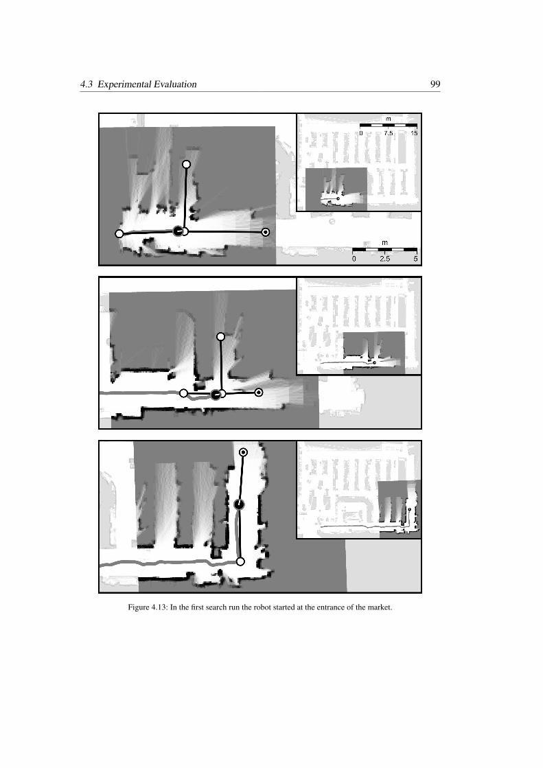
4.3 Experimental Evaluation 99
Figure 4.13: In the first search run the robot started at the entrance of the market.
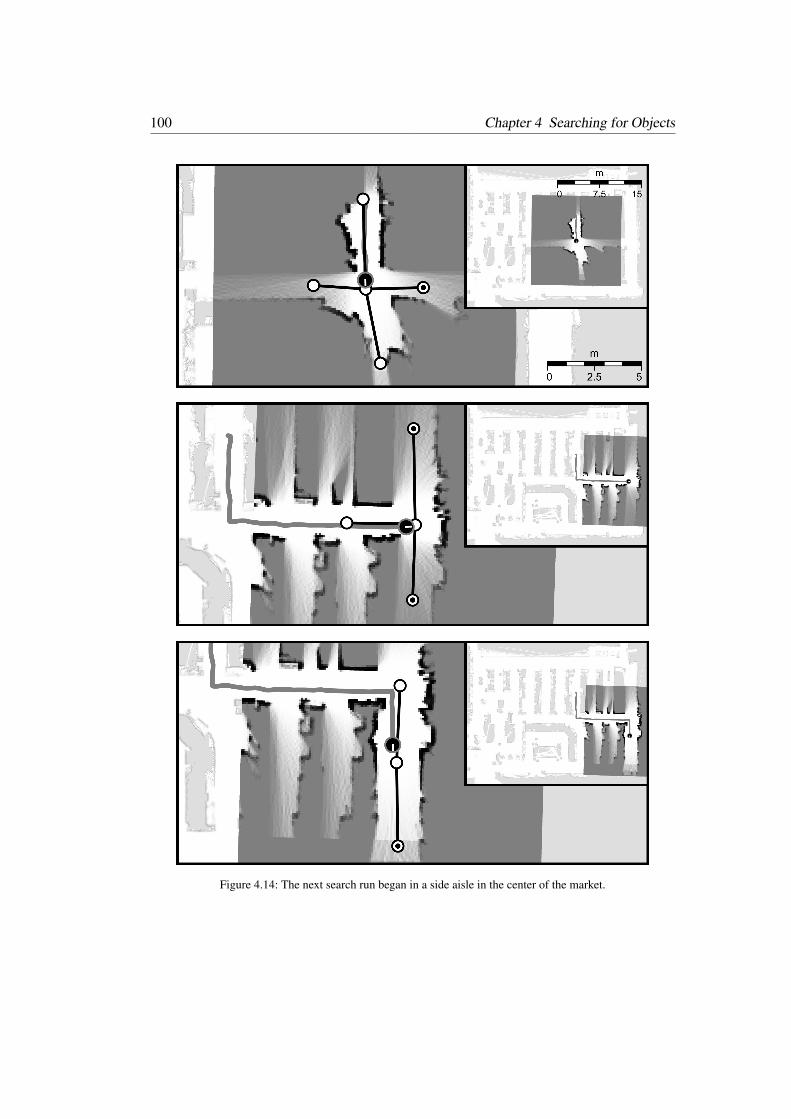
100 Chapter 4 Searching for Objects
Figure 4.14: The next search run began in a side aisle in the center of the market.
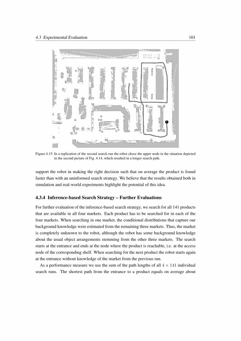
4.3 Experimental Evaluation 101
Figure 4.15: In a replication of the second search run the robot chose the upper node in the situation depictedin the second picture of Fig. 4.14, which resulted in a longer search path.
support the robot in making the right decision such that on average the product is foundfaster than with an uninformed search strategy. We believe that the results obtained both insimulation and real-world experiments highlight the potential of this idea.
4.3.4 Inference-based Search Strategy – Further Evaluations
For further evaluation of the inference-based search strategy, we search for all 141 productsthat are available in all four markets. Each product has to be searched for in each of thefour markets. When searching in one market, the conditional distributions that capture ourbackground knowledge were estimated from the remaining three markets. Thus, the marketis completely unknown to the robot, although the robot has some background knowledgeabout the usual object arrangements stemming from the other three markets. The searchstarts at the entrance and ends at the node where the product is reachable, i.e. at the accessnode of the corresponding shelf. When searching for the next product the robot starts againat the entrance without knowledge of the market from the previous run.
As a performance measure we use the sum of the path lengths of all 4 × 141 individualsearch runs. The shortest path from the entrance to a product equals on average about
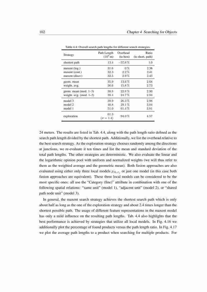
102 Chapter 4 Searching for Objects
Table 4.4: Overall search path lengths for different search strategies.
StrategyPath Length Overhead Ratio
(103 m) (to best) (to short. path)
shortest path 13.4 −57.6% 1.0
maxent (log.) 31.6 0% 2.36maxent (cont.) 32.3 2.2% 2.41maxent (discr.) 32.5 2.9% 2.43
geom. mean 35.9 13.6% 2.68weight. avg. 36.6 15.8% 2.73
geom. mean (mod. 1–3) 38.8 22.8% 2.90weight. avg. (mod. 1–3) 39.4 24.7% 2.94
model 3 39.9 26.3% 2.98model 2 40.8 29.1% 3.04model 1 51.0 61.4% 3.81
exploration61.3
94.0% 4.57(σ = 1.4)
24 meters. The results are listed in Tab. 4.4, along with the path length ratio defined as thesearch path length divided by the shortest path. Additionally, we list the overhead relative tothe best search strategy. As the exploration strategy chooses randomly among the directionsat junctions, we re-evaluate it ten times and list the mean and standard deviation of thetotal path lengths. The other strategies are deterministic. We also evaluate the linear andthe logarithmic opinion pool with uniform and normalized weights (we will thus refer tothem as the weighted average and the geometric mean). Both fusion approaches are alsoevaluated using either only three local models pAi,rj or just one model (in this case bothfusion approaches are equivalent). These three local models can be considered to be themost specific ones: all use the “Category (fine)” attribute in combination with one of thefollowing spatial relations: “same unit” (model 1), “adjacent unit” (model 2), or “sharedpath node unit” (model 3).
In general, the maxent search strategy achieves the shortest search path which is onlyabout half as long as the one of the exploration strategy and about 2.4 times longer than theshortest possible path. The usage of different feature representations in the maxent modelhas only a mild influence on the resulting path lengths. Tab. 4.4 also highlights that thebest performance is achieved by strategies that utilize all local models. In Fig. 4.16 weadditionally plot the percentage of found products versus the path length ratio. In Fig. 4.17we plot the average path lengths to a product when searching for multiple products. For
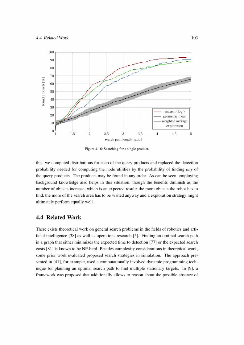
4.4 Related Work 103
1 1.5 2 2.5 3 3.5 4 4.5 50
10
20
30
40
50
60
70
80
90
100
search path length [ratio]
foun
dpr
oduc
ts[%
]
maxent (log.)geometric mean
weighted averageexploration
Figure 4.16: Searching for a single product.
this, we computed distributions for each of the query products and replaced the detectionprobability needed for computing the node utilities by the probability of finding any ofthe query products. The products may be found in any order. As can be seen, employingbackground knowledge also helps in this situation, though the benefits diminish as thenumber of objects increase, which is an expected result: the more objects the robot has tofind, the more of the search area has to be visited anyway and a exploration strategy mightultimately perform equally well.
4.4 Related Work
There exists theoretical work on general search problems in the fields of robotics and arti-ficial intelligence [38] as well as operations research [5]. Finding an optimal search pathin a graph that either minimizes the expected time to detection [77] or the expected searchcosts [81] is known to be NP-hard. Besides complexity considerations in theoretical work,some prior work evaluated proposed search strategies in simulation. The approach pre-sented in [41], for example, used a computationally involved dynamic programming tech-nique for planning an optimal search path to find multiple stationary targets. In [9], aframework was proposed that additionally allows to reason about the possible absence of
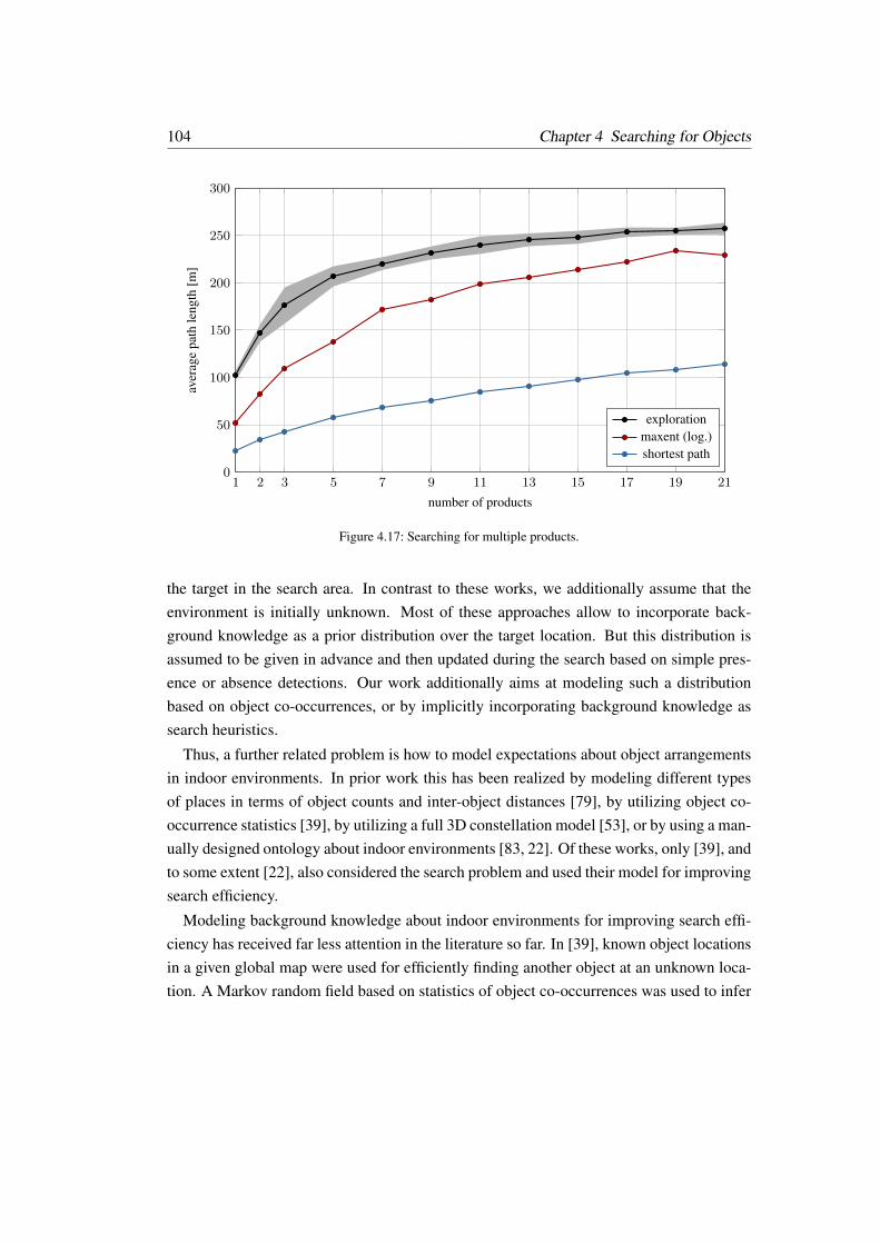
104 Chapter 4 Searching for Objects
1 2 3 5 7 9 11 13 15 17 19 210
50
100
150
200
250
300
number of products
aver
age
path
leng
th[m
]
explorationmaxent (log.)shortest path
Figure 4.17: Searching for multiple products.
the target in the search area. In contrast to these works, we additionally assume that theenvironment is initially unknown. Most of these approaches allow to incorporate back-ground knowledge as a prior distribution over the target location. But this distribution isassumed to be given in advance and then updated during the search based on simple pres-ence or absence detections. Our work additionally aims at modeling such a distributionbased on object co-occurrences, or by implicitly incorporating background knowledge assearch heuristics.
Thus, a further related problem is how to model expectations about object arrangementsin indoor environments. In prior work this has been realized by modeling different typesof places in terms of object counts and inter-object distances [79], by utilizing object co-occurrence statistics [39], by utilizing a full 3D constellation model [53], or by using a man-ually designed ontology about indoor environments [83, 22]. Of these works, only [39], andto some extent [22], also considered the search problem and used their model for improvingsearch efficiency.
Modeling background knowledge about indoor environments for improving search effi-ciency has received far less attention in the literature so far. In [39], known object locationsin a given global map were used for efficiently finding another object at an unknown loca-tion. A Markov random field based on statistics of object co-occurrences was used to infer
4.5 Conclusions 105
a likelihood map and to plan a search path that minimizes the expected search path length.Again, this is a work that assumed that the structure of the environment, and some of theobjects therein, are known. In [10], the application scenario was to efficiently find the en-trance hall in a hotel. A relational navigation policy was learned which utilized informationabout the type of rooms and corridors that are directly connected to the robot’s current loca-tion. The work presented in [22] aimed at improving the task planning of a mobile robot byrelying on semantic information about its domain. In particular, they defined an ontologyabout typical home-like environments and generated plans to find unseen objects or type ofrooms, e.g. a bedroom.
4.5 Conclusions
We presented two approaches for efficiently finding an object in an unknown environment.The first approach is a reactive search technique that only depends on local informationabout the objects in the robot’s vicinity when deciding where to search next. This strategyis based on search heuristics that can be learned from data of optimal search paths. As aproof of concept, we presented real-world experiments in which a mobile robot searchedautonomously for a product using the proposed decision tree strategy. We furthermore pre-sented a second, inference-based search strategy, that explicitly reasons about the locationof the target object given all observations made so far. It thereby takes more global infor-mation into account. The underlying model of this MaxEnt search strategy can be learnedfrom object arrangements of similarly structured example environments.
The MaxEnt strategy achieved shorter search paths than the decision tree strategy. Butthis advantage comes at additional cost as it needs to maintain and update a global map andperform inference by taking into account all previously seen products. This has importantpractical ramifications. The decision tree strategy can be implemented by using a localgrid-map as we have demonstrated in the real-world experiments. Thus, the mapping over-head is constant in the size of the search area – the only exception being the decision pointgraph, which is needed for backtracking to a node with an unvisited edge if all outgoingedges of the current node have been visited already. However, this graph only needs to betopologically correct and the computational overhead during the search can be considerednegligible compared to the maintenance of the local grid-map. The MaxEnt strategy, on theother hand, needs to resort to a computationally much more demanding online SLAM ap-proach for maintaining a consistent global map that preserves the spatial relations between
106 Chapter 4 Searching for Objects
all detected objects. On the downside the mapping overhead now grows linearly with thesize of the search area (or linearly with the length of the path the robot has taken). The up-side is that more informed decisions can be made which eventually leads to shorter searchpaths.
To summarize, in this chapter we presented two general approaches for modeling, learn-ing, and utilizing background knowledge about indoor environments such that a mobilerobot is able to find an object in an initially unknown environment more efficiently thanwould have been possible without such domain-specific knowledge. The choice betweenthese two approaches constitutes a trade-off between the complexity of the underlyingmodel and the resulting search efficiency. Extensive experiments showed that both strate-gies significantly outperform an exploration strategy. This demonstrates the benefits ofutilizing background knowledge when searching for objects in unknown environments.
The inference-based search technique relied on object co-occurrence statistics. The pa-rameters of the model can be learned based on the layout of supermarkets by generatingstatistics about how often certain objects co-occur within a given spatial context. However,these spatial contexts are induced by the local models which use manually defined spatialrelations – like objects being “in the same aisle” or “in the same shelf”. This motivates ourwork in the next chapter, in which we wish to learn the relevant spatial relations betweenobjects in an unsupervised way. Thereby, we hope to increase the autonomy and adaptivityof service robots by side-stepping the reliance on predefined spatial relations derived fromdomain-specific expert knowledge.
CHAPTER 5
Unsupervised Learning of ObjectConstellations
Robots operating in domestic environments need to deal with a variety ofdifferent objects. Often, these objects are neither placed randomly, norindependently of each other. For example, objects on a breakfast tablesuch as plates, knives, or bowls typically occur in recurrent configura-tions. In this chapter, we propose a novel hierarchical generative modelto reason about latent object constellations in a scene. The proposedmodel is a combination of a Dirichlet process and beta processes, whichallows for a probabilistic treatment of the unknown dimensionality of theparameter space. We show how the model can be employed to addressa set of different tasks in scene understanding including unsupervisedscene segmentation and completion of partially specified scenes. Wedescribe how to sample from the posterior distribution of the modelusing Markov chain Monte Carlo (MCMC) techniques and presentan experimental evaluation with simulated as well as real-world dataobtained with a Kinect camera.
Imagine a person laying a breakfast table and the person gets interrupted so that shecannot continue with the breakfast preparation. A service robot, such as the one depictedin Fig. 5.1 on the next page, should be able to proceed laying the table without receivingspecific instructions. It faces a series of questions: how to infer the total number of covers,how to infer which objects are missing on the table, and how should the missing parts be
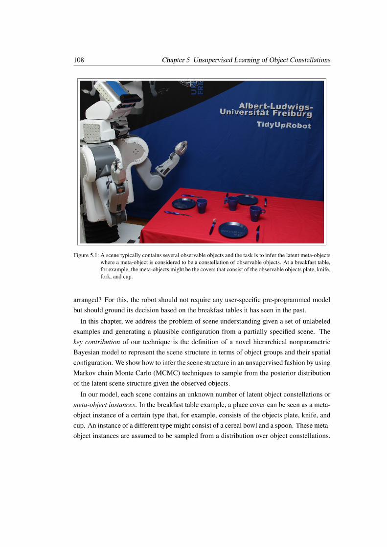
108 Chapter 5 Unsupervised Learning of Object Constellations
Figure 5.1: A scene typically contains several observable objects and the task is to infer the latent meta-objectswhere a meta-object is considered to be a constellation of observable objects. At a breakfast table,for example, the meta-objects might be the covers that consist of the observable objects plate, knife,fork, and cup.
arranged? For this, the robot should not require any user-specific pre-programmed modelbut should ground its decision based on the breakfast tables it has seen in the past.
In this chapter, we address the problem of scene understanding given a set of unlabeledexamples and generating a plausible configuration from a partially specified scene. Thekey contribution of our technique is the definition of a novel hierarchical nonparametricBayesian model to represent the scene structure in terms of object groups and their spatialconfiguration. We show how to infer the scene structure in an unsupervised fashion by usingMarkov chain Monte Carlo (MCMC) techniques to sample from the posterior distributionof the latent scene structure given the observed objects.
In our model, each scene contains an unknown number of latent object constellations ormeta-object instances. In the breakfast table example, a place cover can be seen as a meta-object instance of a certain type that, for example, consists of the objects plate, knife, andcup. An instance of a different type might consist of a cereal bowl and a spoon. These meta-object instances are assumed to be sampled from a distribution over object constellations.

109
(a) Meta-object type. (b) Meta-object instance.
Figure 5.2: A meta-object type is modeled as a collection of parts, each having a Gaussian distribution, amultinomial distribution over object types, and a binary activation probability. A meta-object typeis a distribution over object constellations, which we will call meta-object instances.
We will refer to these distributions as meta-object types (see Fig. 5.2) as we assume thatthere are different types of constellations. Thus, not all meta-object instances of a giventype are the same, they differ in the sense that some objects may be missing and that theobjects may not be arranged in the exact same way.
When specifying a generative model for our problem, we have the difficulty that thedimensionality of the model is part of the learning problem. This means, that besideslearning the parameters of the model, like the pose of a meta-object, we additionally needto infer the number of involved meta-objects, meta-object parts, etc. The standard solutionwould be to follow the model selection approaches, for example, learning several modelsand then choosing the best one. Such a comparison is typically done by trading off the datalikelihood with the model complexity as, for example, done for the Bayesian informationcriterion (BIC). The problem with this approach is the huge number of possible models,which renders this approach intractable in our case.
To avoid this complexity, we follow another approach, motivated by recent developmentsin the field of hierarchical nonparametric Bayesian models based on the Dirichlet processand the beta process. These models are able to adjust their complexity according to thegiven data, thereby sidestepping the need to select among several finite-dimensional modelalternatives. Based on a prior over scenes, which is updated by observed training scenes,the model can be used for parsing new scenes or completing partially specified scenes bysampling the missing objects.
Whereas in this chapter, we consider the problem of learning the object constellationson a breakfast table as depicted in Fig. 5.1, our model is general and not restricted to thisscenario.
110 Chapter 5 Unsupervised Learning of Object Constellations
5.1 Generative Scene Model
In this section, we describe the proposed generative scene model. We assume that the readeris familiar with the basics of nonparametric Bayesian models [23], especially with the Chi-nese restaurant process (CRP) and the Dirichlet process (DP) [70], the (two-parameter)Indian buffet process (IBP) and the beta process (BP) [24, 73], and the concepts of hierar-chical [71] and nested [57] processes in this context.
In the following, we consider a scene as a collection of observable objects representedas labeled points in the 2D plane. The 2D assumption is due to our motivation to modeltable scenes. However, the model is not specifically geared towards 2D data and could inprinciple also be applied to 3D data. Basically, we assume that each scene contains anunknown number of latent object constellations (place covers). An object constellation iscalled a meta-object instance (or simply meta-object) and corresponds to a sample froma meta-object type, which is a distribution over object constellations and is represented asa part-based model with infinitely many parts. As illustrated in Fig. 5.2, each part has abinary activation probability, a Gaussian distribution over the relative object position, anda multinomial distribution over the object type (knife, fork, etc.). To sample from a meta-object type, one first samples the activation of each part. For each activated part, one thensamples the relative position and the object type to be generated at this location. Eachactivated part generates exactly one object per meta-object instance. Thus, the objects of ascene can be grouped into clusters. Each cluster corresponds to a meta-object instance andthe objects of a cluster can be associated to the parts of the corresponding meta-object type.Please note, that we will use the terms “meta-object” and “cover” interchangeably.
5.1.1 Description of the Generative Process
Following the example given in the introduction, imagine that our robot’s goal is to set a ta-ble for a typical family breakfast. At the beginning, it enters a room with an empty breakfasttable and an infinite number of side tables, each holding a prototypical cover. It estimatesthe area A of the breakfast table surface and boldly decides that n ∼ Pois(Aλ) covers arejust right. The robot chooses one of the side tables and finds a note with the address of aChinese restaurant where it can get the cover. Arriving there, it sees again infinitely manytables each corresponding to a particular cover type and each displaying a count of howoften someone took a cover from this table. It is fine with just about any cover type anddecides randomly based on the counts displayed at the tables, even considering a previously
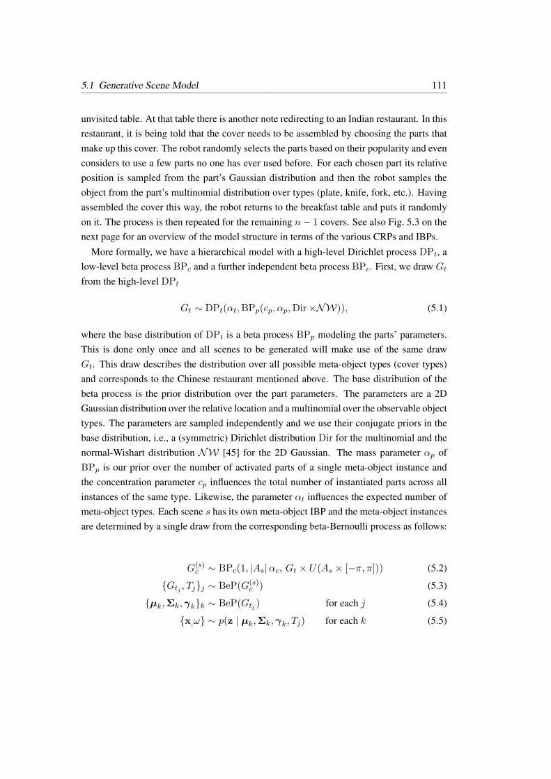
5.1 Generative Scene Model 111
unvisited table. At that table there is another note redirecting to an Indian restaurant. In thisrestaurant, it is being told that the cover needs to be assembled by choosing the parts thatmake up this cover. The robot randomly selects the parts based on their popularity and evenconsiders to use a few parts no one has ever used before. For each chosen part its relativeposition is sampled from the part’s Gaussian distribution and then the robot samples theobject from the part’s multinomial distribution over types (plate, knife, fork, etc.). Havingassembled the cover this way, the robot returns to the breakfast table and puts it randomlyon it. The process is then repeated for the remaining n− 1 covers. See also Fig. 5.3 on thenext page for an overview of the model structure in terms of the various CRPs and IBPs.
More formally, we have a hierarchical model with a high-level Dirichlet process DPt, alow-level beta process BPc and a further independent beta process BPε. First, we draw Gt
from the high-level DPt
Gt ∼ DPt(αt,BPp(cp, αp,Dir×NW)), (5.1)
where the base distribution of DPt is a beta process BPp modeling the parts’ parameters.This is done only once and all scenes to be generated will make use of the same drawGt. This draw describes the distribution over all possible meta-object types (cover types)and corresponds to the Chinese restaurant mentioned above. The base distribution of thebeta process is the prior distribution over the part parameters. The parameters are a 2DGaussian distribution over the relative location and a multinomial over the observable objecttypes. The parameters are sampled independently and we use their conjugate priors in thebase distribution, i.e., a (symmetric) Dirichlet distribution Dir for the multinomial and thenormal-Wishart distribution NW [45] for the 2D Gaussian. The mass parameter αp ofBPp is our prior over the number of activated parts of a single meta-object instance andthe concentration parameter cp influences the total number of instantiated parts across allinstances of the same type. Likewise, the parameter αt influences the expected number ofmeta-object types. Each scene s has its own meta-object IBP and the meta-object instancesare determined by a single draw from the corresponding beta-Bernoulli process as follows:
G(s)c ∼ BPc(1, |As|αc, Gt × U(As × [−π, π])) (5.2)
Gtj , Tjj ∼ BeP(G(s)c ) (5.3)
µk,Σk,γkk ∼ BeP(Gtj ) for each j (5.4)
x,ω ∼ p(z | µk,Σk,γk, Tj) for each k (5.5)
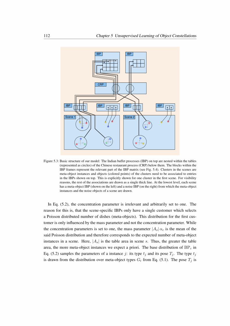
112 Chapter 5 Unsupervised Learning of Object Constellations
Scene 1
IBP
CRP
IBP
IBP
Scene 2
IBP IBP
IBP
Figure 5.3: Basic structure of our model: The Indian buffet processes (IBP) on top are nested within the tables(represented as circles) of the Chinese restaurant process (CRP) below them. The blocks within theIBP frames represent the relevant part of the IBP matrix (see Fig. 5.4). Clusters in the scenes aremeta-object instances and objects (colored points) of the clusters need to be associated to entriesin the IBPs shown on top. This is explicitly shown for one cluster in the first scene. For visibilityreasons, the rest of the associations are drawn as a single thick line. At the lowest level, each scenehas a meta-object IBP (shown on the left) and a noise IBP (on the right) from which the meta-objectinstances and the noise objects of a scene are drawn.
In Eq. (5.2), the concentration parameter is irrelevant and arbitrarily set to one. Thereason for this is, that the scene-specific IBPs only have a single customer which selectsa Poisson distributed number of dishes (meta-objects). This distribution for the first cus-tomer is only influenced by the mass parameter and not the concentration parameter. Whilethe concentration parameters is set to one, the mass parameter |As|αc is the mean of thesaid Poisson distribution and therefore corresponds to the expected number of meta-objectinstances in a scene. Here, |As| is the table area in scene s. Thus, the greater the tablearea, the more meta-object instances we expect a priori. The base distribution of BPc inEq. (5.2) samples the parameters of a instance j: its type tj and its pose Tj . The type tjis drawn from the distribution over meta-object types Gt from Eq. (5.1). The pose Tj is
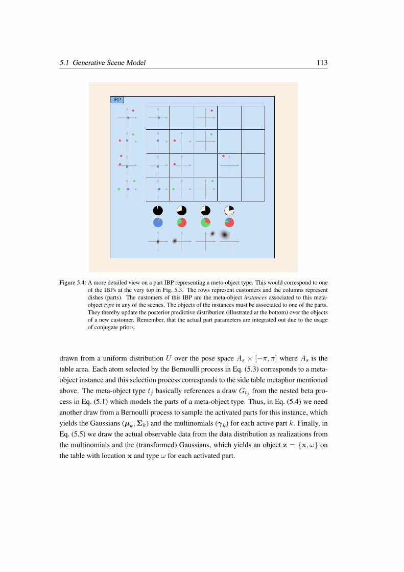
5.1 Generative Scene Model 113
Figure 5.4: A more detailed view on a part IBP representing a meta-object type. This would correspond to oneof the IBPs at the very top in Fig. 5.3. The rows represent customers and the columns representdishes (parts). The customers of this IBP are the meta-object instances associated to this meta-object type in any of the scenes. The objects of the instances must be associated to one of the parts.They thereby update the posterior predictive distribution (illustrated at the bottom) over the objectsof a new customer. Remember, that the actual part parameters are integrated out due to the usageof conjugate priors.
drawn from a uniform distribution U over the pose space As × [−π, π] where As is thetable area. Each atom selected by the Bernoulli process in Eq. (5.3) corresponds to a meta-object instance and this selection process corresponds to the side table metaphor mentionedabove. The meta-object type tj basically references a draw Gtj from the nested beta pro-cess in Eq. (5.1) which models the parts of a meta-object type. Thus, in Eq. (5.4) we needanother draw from a Bernoulli process to sample the activated parts for this instance, whichyields the Gaussians (µk,Σk) and the multinomials (γk) for each active part k. Finally, inEq. (5.5) we draw the actual observable data from the data distribution as realizations fromthe multinomials and the (transformed) Gaussians, which yields an object z = x, ω onthe table with location x and type ω for each activated part.
114 Chapter 5 Unsupervised Learning of Object Constellations
Each scene has an additional independent beta process BPε
G(s)ε ∼ BPε(1, αε,M × U(As)) (5.6)
xi, ωii ∼ BeP(G(s)ε ) (5.7)
that directly samples objects (instead of meta-objects) at random locations in the scene.Here, M is a multinomial over the observable object types and U(As) is the uniform dis-tribution over the table area As. This beta-Bernoulli process will mainly serve as a “noisemodel” during MCMC inference to account for yet unexplained objects in the scene. Ac-cordingly, we set the parameter αε to a rather low value to penalize scenes with manyunexplained objects. Figs. 5.3 and 5.4 illustrate the overall structure of the model.
5.1.2 Posterior Inference in the Model
Some model parameters are integrated out analytically. This holds true for the draws fromthe various processes, which means that we are only working in terms of posterior predic-tive distributions as modeled by the Chinese restaurant and Indian buffet representations.Further, some of the atoms (table and dish parameters) are also integrated out. For example,the dish parameters of the part IBPs consist of Gaussians and multinomials, which can beintegrated out analytically due to the usage of conjugate prior. What remains to be explic-itly represented are the poses and types of the meta-object instances and the associations ofthe observable objects to either the noise process or to a part of a meta-object instance.
We now describe how to sample from the posterior distribution over the latent variablesC,a given the observations z. We use the following notation: The observations are theobjects of all scenes and a single object zi = xi, ωi has a 2D location xi on the tableand a discrete object type ωi. A meta-object instance j has parameters Cj = Tj , tj ,dj,where Tj denotes the pose and tj denotes the meta-object type, which is an index to a tablein the type CRP, and dj denotes part activations and associations to the observable objects.If dj,k = 0 then part k of meta-object instance j is inactive, where k is an index to a dishin the corresponding part IBP (which is nested in the CRP table tj). Otherwise, the partis active and dj,k 6= 0 is a reference to the associated observable object, i.e., dj,k = i if itgenerated the object zi. Next, for each scene we have the associations a to the noise IBP,i.e., the list of objects currently not associated to any meta-object instance. For ease ofnotation, we will use index functions [·] in an intuitive way, for example, t[−j] denotes alltype assignments except the type assignment tj of meta-object j, and T[tj ] denotes all poses
5.1 Generative Scene Model 115
of meta-objects that have the same type tj as meta-object j, and z[d] are all observationsreferenced by the associations d, etc.
We employ Metropolis-Hastings (MH) moves to sample from the posterior [2], whichallows for big steps in the state space by updating several strongly correlated variables at atime. In the starting state of the Markov chain, all objects are assigned to the noise IBP oftheir respective scene and thus are interpreted as yet unexplained objects. We sample for afixed yet sufficiently high number of iterations to be sure that the Markov chain converged.We use several types of MH moves, which we will explain in detail after describing thejoint distribution.
5.1.2.1 Joint Distribution
The joint distribution p(C,a, z) = p(T, t,d,a, z) is defined in terms of the CRP and IBPrepresentation where the draws from the processes have been integrated out. It includesthe poses T of all meta-object instances, their types t (table indices of the type CRP), theiractive parts d (dish indices of the corresponding part IBP), the associations a of objects tothe noise process, and the observed data z.
p(C,a, z) = p(T, t,d,a, z) (5.8)
=
(S∏s=1
p(ns,ε)p(ns,m)
)p(t)
(nt∏t=1
p(d[t] | t)
)
p(T)
(nt∏t=1
Kt∏k=1
p(z[d[t,k]] | T[t],d[t,k], t)
)(5.9)
Here, ns,m is the number of meta-object instances and ns,ε is the number of noise objectsin scene s. Each dish parameter of the noise IBP directly corresponds to the parameterszi = xi, ωi of the associated noise object, as we assumed that there is no data distributionassociated with these dishes. The base distribution for the dish parameters consists ofindependent and uniform priors over the table area and the object types, and so each dishparameter has the likelihood (nω |As|)−1, where nω is the number of observable objecttypes and |As| is the area of the table in scene s. Thus, the probability of the objects z[a[s]]
associated to a scene’s noise IBP only depends on the number of noise objects and noton the particular type or position of these objects. However, it would be straightforwardto use a non-uniform base distribution. Denoting the Poisson distribution with mean λ as

116 Chapter 5 Unsupervised Learning of Object Constellations
Pois(· | λ) we thus have
p(ns,ε) = p(z[a[s]],a[s]) = ns,ε! Pois(ns,ε | αε)(nω |As|)−ns,ε . (5.10)
Next, p(ns,m) = ns,m! Pois(ns,m | αm |As|) is the prior probability for having ns,m meta-objects in scene s. The dish parameters of a meta-object IBP are the meta-object parametersCj , consisting of the pose, type, and part activations. The likelihood for sampling a posep(Tj) = (|As| 2π)−1 is uniform over the table surface and uniform in orientation, hencep(T) =
∏Ss=1(|As| 2π)−ns,m . Next, p(t) is the CRP prior for the meta-object types of all
meta-object instances. The factors p(d[t] | t) are the IBP priors for the part activations forall meta-object instances of type t and there are nt different types currently instantiated.During MCMC sampling, we will only need the conditional for a single meta-object j
p(tj ,dj | t[−j],d[−j]) = p(dj | d[−j,tj ], t)p(tj | t[−j]). (5.11)
Here, p(tj | t[−j]) is the CRP predictive distribution
p(tj = i | t[−j]) =
ni
αc +∑
i′ ni′i is an existing type
αcαc +
∑i′ ni′
i is a new type, (5.12)
and ni is the number of meta-object instances of type i (not counting instance j) and αcis the concentration parameter of the CRP. Further, p(dj | d[−j,tj ], t) is the predictivedistribution of the two-parameter IBP, which factors into activation probabilities for eachof the existing parts and an additional factor for the number of new parts, denoted as n+.An existing part is a part that has been activated by at least one other meta-object instanceof this type in any of the scenes. The activation probability for an existing part k is
p(dj,k 6= 0 | d[−j,tj ], t) =nk
ntj + cp, (5.13)
where cp is the concentration parameter of the part IBP, nk is the number of meta-objectinstances that have part k activated in any of the scenes, and ntj is the total number ofmeta-object instances of type tj in all scenes (the counts exclude the meta-object j itself).The probability for having n+ associations to new parts is
p(d[j,+] | d[−j,tj ], t) = n+! Pois
(n+
∣∣∣∣ cpαpntj + cp
), (5.14)
5.1 Generative Scene Model 117
where αp is the mass parameter of the part IBP, and d[j,+] denotes the associations to newparts.
As stated in Eq. (5.8), the data likelihood p(z[d] | T,d, t) for the objects associatedto meta-objects factors into likelihoods for each individual part k. Further, it factors intoa spatial component and a component for the observable object type. As the meta-objectposes T are given, we can transform the absolute positions x[d[t,k]] of the objects associ-ated to a certain part k of meta-object type t into relative positions x[d[t,k]] with respect toa common meta-object reference frame. The relative positions are assumed to be sampledfrom the part’s Gaussian distribution which in turn is sampled from a normal-Wishart dis-tribution. As the Gaussian and the normal-Wishart distribution form a conjugate pair, wecan analytically integrate out the part’s Gaussian distribution which therefore does not haveto be explicitly represented. Hence, the joint likelihood for x[d[t,k]] of part k is computed asthe marginal likelihood under a normal-Wishart prior. During MCMC inference, we onlyneed to work with the posterior predictive distribution
p(x[dj,k] | x[d[−j,tj ,k]]) = tν(x[dj,k] | µ,Σ) (5.15)
for a single relative position given the rest. This is a multivariate t-distribution tν with pa-rameters µ,Σ depending both on x[d[−j,tj ,k]]
and the parameters of the normal-Wishart prior– for details see [45] and Section A.1 in the appendix. Similarly, the part’s multinomial dis-tribution over the observable object types can be integrated out as it forms a conjugate pairwith the Dirichlet distribution. The posterior predictive distribution for a single object typeis
p(ω[dj,k] | ω[d[−j,tj ,k]]) =
nω + αω∑ω′(nω′ + αω′)
, (5.16)
where nω is the number of times an object of type ω has been associated to part k of thismeta-object type tj , and αω is the pseudo-count of the Dirichlet prior. When describingthe MCMC moves, we will sometimes make use of the predictive likelihood for all objectsz[dj ] associated to a single meta-object instance j. This likelihood factors into the posteriorpredictive distributions of the individual parts and their spatial and object type components,as described above. In the following, we will describe the various MCMC moves in detail.
5.1.2.2 Death (Birth) Move (Tj , tj ,dj ,a)→ (a?)
A death move selects a meta-object j uniformly at random, adds all of its currently asso-ciated objects to the noise process and removes the meta-object j from the model. The
118 Chapter 5 Unsupervised Learning of Object Constellations
proposal probability for this move is qd(C−j ,a? | Cj ,C−j ,a) = (nm)−1 where nm de-notes the number of instantiated meta-objects in this scene before the death move. Tosimplify notation, we will just write qd(Cj) for the probability of deleting meta-object j.The reverse proposal is the birth proposal qb(C?j ,C−j ,a
? | C−j ,a, z) that proposes newparameters C?j = T ?j , t?j ,d
?j for an additional meta-object: the pose T ?j , the type t?j ,
and the associations d?j . The new meta-object may reference any of the objects previouslyassociated to the noise process and any non-referenced noise objects remain associated tothe noise process. We will describe the details of the birth proposal in detail later on. Tosimplify notation, we will just write qb(Cj) for the birth proposal. Plugging in the modeland proposal distributions in the MH ratio and simplifying we arrive at the acceptance ratioof the death move
Rd =1
p(z[dj ] | z[d[−j,tj ]],T[tj ],d[tj ], t)p(tj ,dj | t[−j],d[−j])
1
p(Tj)
p(nm − 1)
p(nm)
p(nε + nj)
p(nε)
qb(Cj)
qd(Cj). (5.17)
The counts nj , nm, and nε refer to the state before the death move, and nm denotes thenumber of meta-objects in this scene, nj are the number of objects currently associated tometa-object j, and nε is the number of noise objects. The ratio of a birth move is derivedsimilarly.
5.1.2.3 Switch Move (Tj , tj ,dj ,a)→ (T ?j , t?j ,d
?j ,a
?)
This move is a combined death and birth move. It removes a meta-object and then proposesa new meta-object using the birth proposal. Thus, the number of meta-objects remains thesame but one meta-object simultaneously changes its type tj , pose Tj , and part associationsdj . The death proposals cancel out and the acceptance ratio of this move is
Rs =p(z[d?j ] | z[d[−j,t?
j]], T ?j ,T[−j,t?j ],d
?j ,d[−j,t?j ], t
?j , t[−j])
p(z[dj ] | z[d[−j,tj ]], Tj ,T[−j,tj ],dj ,d[−j,tj ], tj , t[−j])
p(t?j ,d?j | t[−j],d[−j])p(T
?j )p(n?ε )qb(Cj)
p(tj ,dj | t[−j],d[−j])p(Tj)p(nε)qb(C?j ). (5.18)
5.1 Generative Scene Model 119
5.1.2.4 Shift Move (Tj)→ (T ?j )
This move disturbs the pose Tj of a meta-object by adding Gaussian noise to it while thetype and part associations remain unchanged. The acceptance ratio depends only on thespatial posterior predictive distributions of the objects associated to this meta-object. Theproposal likelihoods cancel due to symmetry and the final ratio is
RT =p(x[dj ] | x[d[−j,tj ]]
, T ?j ,T[−j,tj ],d[tj ], t)p(T ?j )
p(x[dj ] | x[d[−j,tj ]], Tj ,T[−j,tj ],d[tj ], t)p(Tj)
. (5.19)
5.1.2.5 Association Move (Existing Part) (dj ,a)→ (d?j ,a?)
This move samples the part activation and object association of an existing part k of asingle meta-object j. In the IBP metaphor, this corresponds to sampling the selection of asingle existing dish (part) for a single customer (meta-object instance). If the existing partis already associated with an object, we consider this object to be temporarily re-associatedto the noise process (such that there are now nε noise objects). We then use Gibbs samplingto obtain one of nε + 1 possible associations: either the part k is inactive (dj,k = 0) andnot associated with any object on the table, or it is active (dj,k 6= 0) and associated withone out of nε currently available noise objects of this scene (e.g. zi when dj,k = i). Theprobabilities for these cases are proportional to
p(dj,k = i) ∝p(dj,k = 0 | d[−j,tj ,k], t)p(nε) i = 0
p(zi | z[d[−j,tj ,k]],T[tj ], dj,k,d[−j,tj ,k], t)
p(dj,k 6= 0 | d[−j,tj ,k], t)p(nε − 1)i 6= 0
(5.20)
5.1.2.6 Association Move (New Parts) (dj ,a)→ (d?j ,a?)
This move samples the associations of objects to new parts. For this, we use two comple-mentary Metropolis-Hastings moves: one move increases the number of new parts by oneby assigning a noise object to a new part, while the other move decreases the number ofnew parts by one by assigning an associated object (of a new part) to the noise process. Theacceptance ratio for removing object zi from a new part k of meta-object j that currently

120 Chapter 5 Unsupervised Learning of Object Constellations
has n+ new parts is
R− =1
p(zi | Tj , dj,k)p(d?[j,+] | d[−j,tj ], t)
p(d[j,+] | d[−j,tj ], t)
p(nε + 1)
p(nε)
q+
q−(5.21)
The proposal q− = (n+)−1 chooses one of the new parts to be removed uniformly atrandom, while the reverse proposal q+ = (nε + 1)−1 chooses uniformly at random one ofthen nε + 1 noise objects to be associated to a new part. The MH move that increases thenumber new parts is derived similarly.
5.1.2.7 Birth Proposal qb(Tj , tj ,dj)
The birth, death, and switch moves rely on a birth proposal that samples new meta-objectparameters Cj = Tj , tj ,dj. The general idea is to sample the pose Tj and type tj in afirst step. We then proceed to sample the associations dj given Tj and tj , i.e., the potentialassignment of noise objects to the parts of this meta-object.
Sampling Tj and tj is done in either of two modes: the object mode or the matchingmode. In object mode, we choose an object uniformly at random and center the meta-objectpose Tj at the object’s location (with random orientation) and add Gaussian noise to it. Thetype tj is sampled from the current predictive distribution of the type CRP. In contrast, thematching mode was inspired by bottom-up top-down approaches and aims to propose Tjand tj in a more efficient way by considering the currently instantiated meta-object typesin the model. However, in contrast to the object mode, it cannot propose new meta-objecttypes (new tables in the type CRP). It selects two objects and associates them to a suitablepart pair. This suffices to define the pose Tj as the corresponding transformation of theseparts into the scene. In detail, we first sample one of the objects zi at random and chooseits nearest neighbor zj . We match this ordered pair 〈zi, zj〉 against all ordered part pairs〈ki′ , kj′〉 of the meta-object types to obtain their matching probabilities pm with respectto the parts’ posterior predictive means, µi′ and µj′ , of the spatial distribution, and theirposterior predictive distributions, Mi′ and Mj′ , over the observable object types ωi and ωj
pm(〈ki′ , kj′〉 | 〈zi, zj〉) ∝ N (d∆ | 0, σ2m)Mi′(ωi)Mj′(ωj). (5.22)
Here, d∆ = ‖xi − xj‖ − ‖µi′ − µj′‖ is the residual of the objects’ relative distance w.r.t.the distance of the posterior means and σ2
m is a fixed constant. We then sample a part pair〈ki′ , kj′〉 according to its matching probability to define, together with the objects zi and

5.2 Experiments 121
zj , the pose Tj . Finally, we add Gaussian noise to Tj . The sampled part pair implicitlydefines the meta-object type tj .
After having sampled Tj and tj using either of these two modes, the next step is to samplethe associations dj . For this, we randomly choose, without repetition, a noise object anduse Gibbs sampling to obtain its association to either: (a) a yet unassociated part of themeta-object instance; (b) a new part of the meta-object instance; or (c) be considered anoise object. The probabilities for (a) and (b) are proportional to the spatial and objecttype posterior predictive distributions of the respective parts, while (c) is based on the noiseIBP’s base distribution.
Besides sampling from the proposal distribution we also need to be able to evaluate thelikelihood qb(Cj) for sampling a given parameter set Cj . For this, we need to marginalizeover the latent variables of the proposal, e.g. the binary mode variable (object mode ormatching mode), the chosen object zi, and the chosen part pair of the matching mode.
5.2 Experiments
We tested our model on both synthetic data and on real-world data acquired with a Kinectcamera.
5.2.1 Synthetic Data
In the synthetic data experiment, table scenes were generated automatically using a differ-ent, hand-crafted generative model. We generated 25 training scenes ranging from two tosix covers. The cover types represent two different breakfast types. The first type consistsof a cereal bowl and a spoon, while the second type consists of a plate with a glass, a forkand a knife. A fork can be randomly placed at the right or the left of a plate or being absent.
The latent parameters are inferred using all the generated training scenes and setting thehyperparameters to αε = 0.5, cp = 0.25, αp = 2.5, αt = 5, and αc = 1. As a first test, wewanted to show that the model is able to segment the scenes in a consistent and meaningfulway. The results of this test are shown in Fig. 5.5a. A set of different scenes are segmentedby using the learned model. We see that each scene has been segmented with the samecover types and objects are correctly clustered. Note that the color of the meta-objects andof the parts can change in every run, since the ordering of types and meta-objects is notrelevant in our model. What is important is that the topological and metrical configurationare respected.

122 Chapter 5 Unsupervised Learning of Object Constellations
(a) Examples of parsed scenes of the synthetic data set.
(b) Examples of parsed scenes of the real-world data set.
Figure 5.5: The picture shows the inferred meta-objects with their part relationships. Each picture shows adifferent scene from a different MCMC run. The color of the spheres correspond to the meta-objecttype. The color of the vertical lines indicates the part of the corresponding meta-object type thatthe object on the table is currently associated with.
A second test is to see if the model can infer the meta-objects in incomplete scenes andif it is able to complete them. To this end, we artificially eliminated objects from alreadygenerated scenes and segmented the altered scene again using the learned model. We dis-covered that the approach was able to infer the correct cover type even in the absence ofthe missing object. As can be seen in Fig. 5.6a, the approach correctly segmented and rec-ognized the meta-objects and is aware of the missing plate (the red branch of the hierarchythat is not grounded on an existing object). The missing object can then be inferred bysampling from the part’s posterior predictive distribution over the location and type of themissing object, as the one shown in Fig. 5.7 (left) on page 124.
5.2.2 Real-world Data
We used a Microsoft Kinect depth camera to identify the objects on the table by, first,segmenting the objects by subtracting the table plane in combination with a color-based
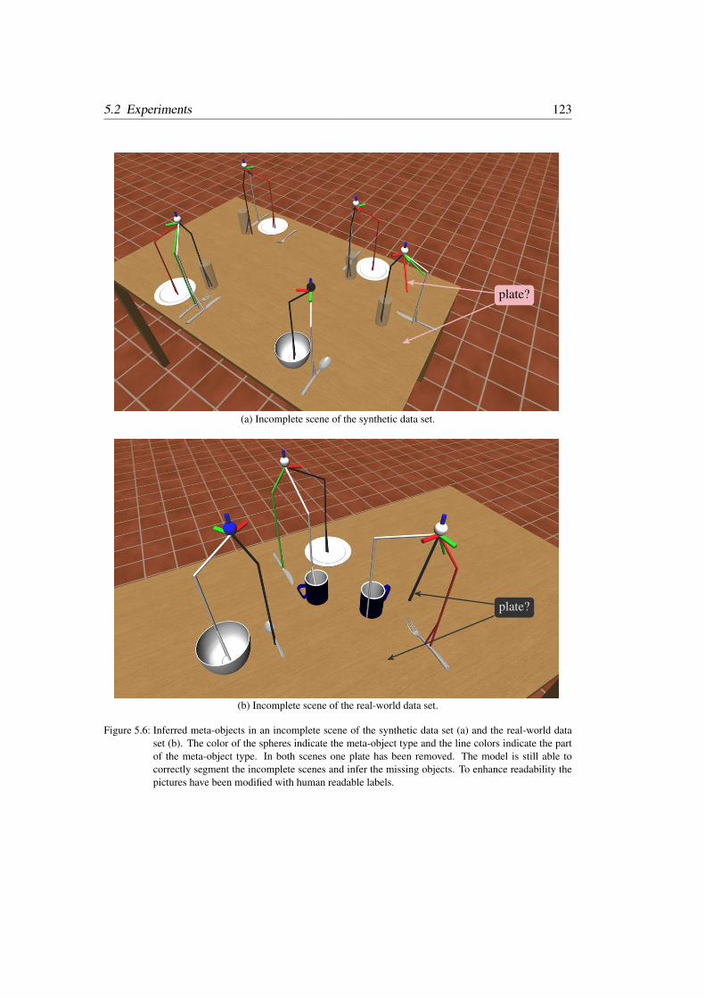
5.2 Experiments 123
plate?
(a) Incomplete scene of the synthetic data set.
plate?
(b) Incomplete scene of the real-world data set.
Figure 5.6: Inferred meta-objects in an incomplete scene of the synthetic data set (a) and the real-world dataset (b). The color of the spheres indicate the meta-object type and the line colors indicate the partof the meta-object type. In both scenes one plate has been removed. The model is still able tocorrectly segment the incomplete scenes and infer the missing objects. To enhance readability thepictures have been modified with human readable labels.

124 Chapter 5 Unsupervised Learning of Object Constellations
−0.2 −0.1 0 0.1 0.2
−0.2
−0.1
0
0.1
0.2
[m]
[m]
part 10.99 activation prob.0.99 glass
part 20.99 activation prob.0.99 knife
part 30.99 activation prob.0.99 plate
part 40.62 activation prob.0.99 fork
−0.2 −0.1 0 0.1 0.2
[m]
part 20.97 activation prob.0.99 cup
part 10.97 activation prob.0.99 knife
part 30.86 activation prob.0.99 plate
Figure 5.7: Examples of spatial posterior predictive distributions of several parts of a cover type and theiractivation probabilities and most likely observable object types. The cover type on the left waslearned on synthetic data, while the one on the right was learned on the real-world data set.
segmentation. Second, we detect the objects based on the segmented pointclouds using astraight forward feature-based object detection system with a cascade of one-vs-all classi-fiers. An example for the segmentation and object identification is shown in Fig. 5.8. Notethat there are likely to be better detection systems, however, the task of detecting the objectson the table is orthogonal to the scientific contribution of our proposed technique.
The same tests performed on the synthetic data have been performed also in this case,showing basically the same results. In particular, Fig. 5.5b shows the segmentation results,Fig. 5.6b shows a modified scene where a plate has been removed and Fig. 5.7 (right) showsthe posterior predictive distribution for location and type, as for the synthetic case, that canbe used to complete an incomplete scene.
To better illustrate the inference process, we plot the log-likelihood, the total number ofparts, and the total number of meta-object types in Fig. 5.9 on page 126 as they evolveduring MCMC sampling.
5.3 Related Work
In this section we describe the relevant works on unsupervised scene analysis. A first familyof approaches, and the most related to our model, employs nonparametric Bayesian models
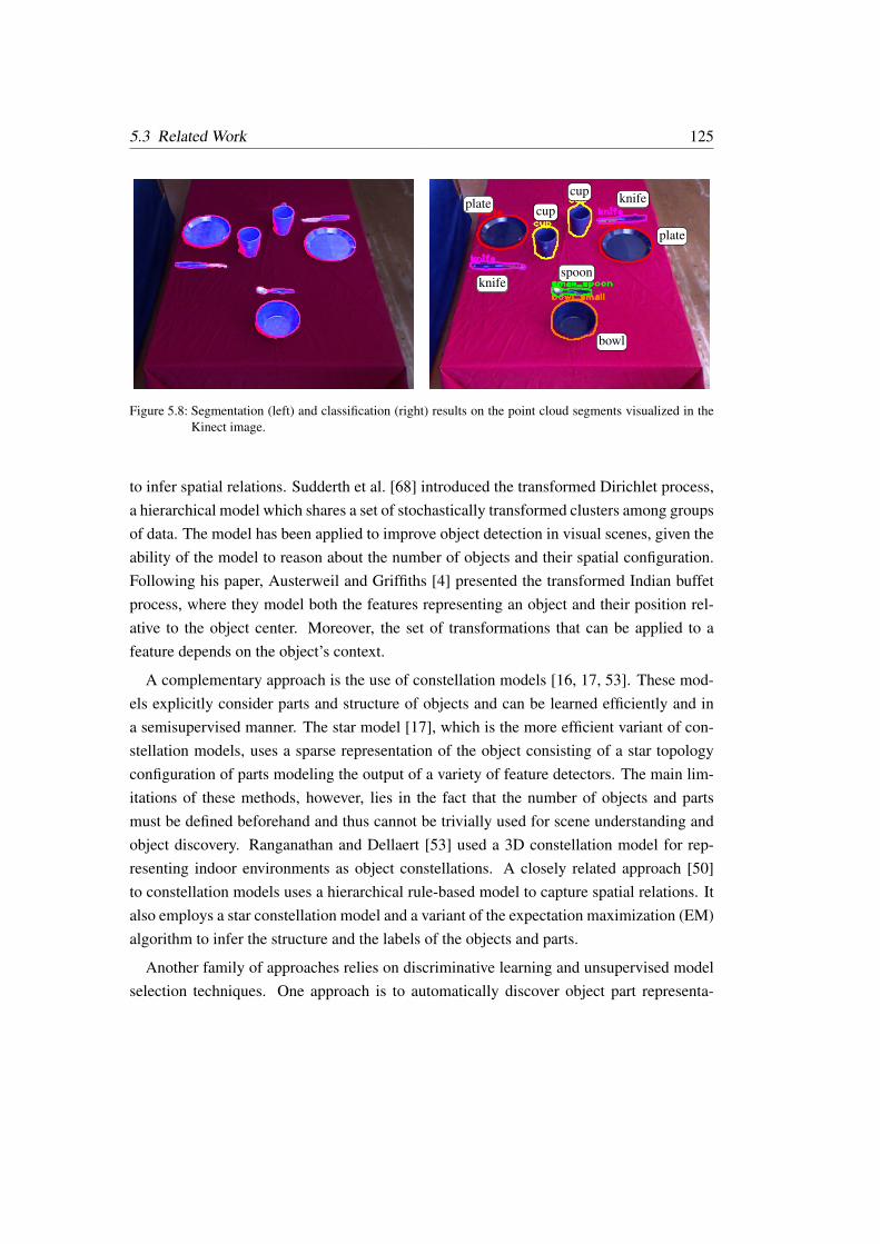
5.3 Related Work 125
knife
plate cup
cup knife
plate
spoon
bowl
Figure 5.8: Segmentation (left) and classification (right) results on the point cloud segments visualized in theKinect image.
to infer spatial relations. Sudderth et al. [68] introduced the transformed Dirichlet process,a hierarchical model which shares a set of stochastically transformed clusters among groupsof data. The model has been applied to improve object detection in visual scenes, given theability of the model to reason about the number of objects and their spatial configuration.Following his paper, Austerweil and Griffiths [4] presented the transformed Indian buffetprocess, where they model both the features representing an object and their position rel-ative to the object center. Moreover, the set of transformations that can be applied to afeature depends on the object’s context.
A complementary approach is the use of constellation models [16, 17, 53]. These mod-els explicitly consider parts and structure of objects and can be learned efficiently and ina semisupervised manner. The star model [17], which is the more efficient variant of con-stellation models, uses a sparse representation of the object consisting of a star topologyconfiguration of parts modeling the output of a variety of feature detectors. The main lim-itations of these methods, however, lies in the fact that the number of objects and partsmust be defined beforehand and thus cannot be trivially used for scene understanding andobject discovery. Ranganathan and Dellaert [53] used a 3D constellation model for rep-resenting indoor environments as object constellations. A closely related approach [50]to constellation models uses a hierarchical rule-based model to capture spatial relations. Italso employs a star constellation model and a variant of the expectation maximization (EM)algorithm to infer the structure and the labels of the objects and parts.
Another family of approaches relies on discriminative learning and unsupervised modelselection techniques. One approach is to automatically discover object part representa-

126 Chapter 5 Unsupervised Learning of Object Constellations
−1,000
0
1,000
log-
likel
ihoo
d
0
10
20
met
a-ob
ject
part
s
0 500 1,000 1,500 2,000 2,500 3,000 3,500 4,000 4,500 5,000 5,500 6,000 6,500
0
2
4
6
MCMC sampling iteration
met
a-ob
ject
type
s
Figure 5.9: The plots depict the log-likelihood, the total number of meta-object parts (summed over all meta-object types), and the number of meta-object types as they evolve during MCMC sampling. Thered lines corresponds to the synthetic data set and the blue lines to the real-world data set.
5.4 Conclusion 127
tions [61]. In this work, the authors introduced a latent conditional random field (CRF)based on a flexible assembly of parts. Individual part labels are modeled as hidden nodesand a modified version of the EM algorithm has been developed for learning the pairwisestructure of the underlying graphical model. Triebel et al. [76] presented an unsupervisedapproach to segment 3D range scan data and to discover objects by the frequency of theappearance of their parts. The data is first segmented using graph-based clustering, theneach segment is treated as a potential object part. The authors used CRFs to representboth the part graph to model the interdependence of parts with object labels, and a scenegraph to smooth the object labels. Spinello et al. [66] proposed an unsupervised detectiontechnique based on a voting scheme of image descriptors. They introduced the concept oflatticelets: a minimal set of pairwise relations that can generalize the patterns connectiv-ity. Conditional random fields are then used to couple low level detections with high levelscene description. Jiang et al. [32] used an undirected graphical model to infer the bestplacement for multiple objects in a scene. Their model considers several features of objectconfigurations, such as stability, stacking, and semantic preferences.
A different approach is the one of Fidler and Leonardis [20]. They construct a hierar-chical representation of visual input using a bottom-up strategy. They learn the statisticallymost significant compositions of simple features with respect to more complex higher levelones. Parts are learned sequentially, layer after layer. Separate classification and groupingtechnique are used for the bottom and top layers to account for the numerical difference(sensor data) and semantical ones (object category).
The novelty of the approach presented in this chapter lies in the combination of a Dirich-let process and beta-Bernoulli processes which provides us with a prior for sampling orcompleting entire scenes.
5.4 Conclusion
In this chapter, we presented a novel and fully probabilistic generative model for unsuper-vised scene analysis. Our approach is able to model the spatial arrangement of objects. Itmaintains a nonparametric prior over scenes, which is updated by observing scenes and candirectly be applied for parsing new scenes and for model completion by inferring missingobjects in an incomplete scene. Our model applies a combination of a Dirichlet process andbeta processes, allowing for a probabilistic treatment of the model complexity. In this way,we avoid a model selection step, which is typically intractable for the models considered

128 Chapter 5 Unsupervised Learning of Object Constellations
here. To evaluate our approach, we successfully used our approach to infer missing objectsin complex scenes.
This chapter concludes the technical description of the main contributions of this thesis.In the next chapter, we will shortly recapitulate the achieved results and discuss directionsfor future research.

CHAPTER 6
Discussion
We recapitulate the main contributions of this thesis: (a) RFID-basedobject localization, (b) searching for objects in unknown environments,and (c) learning spatial relations between objects. Further, we describeseveral open research questions that we have identified during our workon the techniques presented in this thesis and discuss directions forfuture research.
In this thesis, we presented several novel techniques for (a) localizing objects, (b) search-ing for objects in unknown environments, and (c) learning spatial relations between objectsin an unsupervised way. Our initial motivation for addressing these topics was the assump-tion that if robots should be able to perform useful tasks in domestic environments in anadaptive and efficient manner, then they need to be aware of the object-related concepts thatinfluence the structural organization of these environments. That is, robots should be ableto acquire and utilize a representation of their environment that takes into account the spa-tial context and interdependencies between objects. We showed that such representationsenable a robot to perform tasks more efficiently or to address completely new tasks. Forexample, a robot might reason about missing or misplaced objects or it can search moreefficiently for an object if it has some prior knowledge about usual object arrangements.Further, we argued that it would be desirable that a robot is able to acquire this knowledgein an unsupervised way.
However, as a precondition for the ability to search for objects or to learn relevant objectrelations, a robot needs to localize the objects in the first place. As future retail productsmay already be equipped with RFID tags, we considered the problem of RFID-based object
130 Chapter 6 Discussion
localization. For this, we presented a novel combined sensor model that utilizes both thereceived signal strength and tag detections of RFID systems for localizing the RFID tags.Further, we showed that this sensor model can also be employed in a particle filter forself-localization of the robot when given a map of tag locations. The manual acquisitionof calibration data for setting up the sensor model can be a tedious and time-consumingtask in practice. We therefore proposed a technique to learn such a model in an iterativeand unsupervised way, which greatly simplifies this calibration phase. The learning phaseiterates between two steps: (a) localizing the RFID tags with a given sensor model and(b) learning a sensor model with a given list of tag locations. As a side effect, this iterativeprocedure thereby not only learns a sensor model in an unsupervised way, but also estimatesthe tag locations. Once we have learned a sensor model we can localize RFID tags in anon-iterative way. For further evaluation of our technique, we implemented a sensor modelthat has been shown to be effective for WiFi localization and we compared the accuracyof both techniques. Further, we described how the WiFi model can be improved in thecontext of RFID localization by mapping the signal strength in pose space rather than in2D. We performed experiments in several real-world settings and compared our approachto other state-of-the-art techniques. The results showed that our approach achieves thecomputational efficiency of existing sensor-centric models and an accuracy of a state-of-the-art approach that learns a location-dependent model for each tag.
Given that we can localize objects, we moved on to address the question how knowledgeabout usual object arrangements can be learned and represented in such a way that a robotis able to more efficiently find an object in an unknown but similarly structured environ-ment. For this, we proposed and evaluated two novel techniques and considered the searchfor a product in a supermarket as an illustrative example. The first approach is a reactivesearch technique and emphasizes the sequential nature of the search process, which is asequential decision making process. Being in a certain state the robot must choose among aset of available actions, i.e., at junctions in the supermarket the robot has to decide where tosearch next. For this, we learned a state-to-action mapping, a policy, where a state includesthe currently observed objects in direction of the different aisles and the available actionscorrespond to the aisle the robot may choose to visit next. To learn this state-to-action map-ping, we draw on ideas from imitation learning. We generated examples of optimal searchbehavior by computing the shortest path from a starting location to the product. In eachvisited state of a demonstrated example path, the robot takes a certain action and discardsthe other available actions in this state. Thereby, it provides positive and negative examplesof state-action pairs to be taken or not, respectively. We used this data to learn a decision

131
tree for state-action pairs, which yields a classifier-based policy representation. This re-sulted in compact policy representations that resemble search heuristics. These heuristicswere learned on a training set of three supermarkets and were then evaluated in a fourthsupermarket.
Our second approach treats the search problem as an inference problem. Thus, insteadof reactively mapping observations to actions as in our first approach, we first computea distribution over the possible locations of the target object given the thus far observedobjects and the partially known structure of the environment. The robot then chooses thenext goal location by trading off the probability of finding the object there with the costs ofmoving to this location. Each time new information becomes available, i.e., newly detectedobjects or newly discovered parts of the environment, the robot recomputes the distribution.Basically, this approach encodes the relevant background knowledge as expectations abouthow objects co-occur. However, co-occurrence of objects can only be defined with regardto a spatial context – like objects being “in the same aisle”, or one object being “in theneighboring aisle” of the other. Each particular spatial context induces a different localco-occurrence model. Motivated by the idea of combining an ensemble of base classifiersto form a more robust classifier, we used a diverse set of local co-occurrence models, eachconsidering a different spatial relation, and fused their outcomes as features in a maximumentropy model, which in our case models the discrete distribution over all possible locationsof the target object.
We performed extensive experiments and compared both of our search techniques to abaseline approach and to the performance of humans. Our evaluation showed, that theinference-based search technique yielded shorter search paths than the approach based onsearch heuristics. Both search techniques significantly outperform a baseline strategy thatexplores the environment until it finds the product but does not consider any other infor-mation except the distinction between visited and non-visited areas. This demonstrates thebenefits of utilizing background knowledge when searching for objects in unknown envi-ronments. We additionally compared our approaches to the search efficiency of humansubjects in a real supermarket. Roughly speaking, our inference-based search techniquewas able to halve the average search path length when compared to the exploration strat-egy, while the humans were able to top our approaches by again halving the average searchpath length when compared to our inference-based search technique.
Our inference-based search technique basically relied on object co-occurrence statistics.However, the spatial context within which objects could co-occur was manually given bythe predefined spatial relations – like objects being “in the same aisle” or “in the same
132 Chapter 6 Discussion
shelf”. In our last contribution of this thesis, we took the learning scenario one step furtherby simultaneously learning both the spatial context and the co-occurrence of objects withina spatial context. That is, we learned spatially coherent object constellations in multi-objectscenes in an unsupervised way. As an application scenario we considered tabletop scenesand our goal was to learn the different object constellations that correspond to the place cov-ers consisting of, e.g., a plate, a knife, and a mug. For this, we presented a novel and fullyprobabilistic generative model for unsupervised scene analysis. Our approach maintains anonparametric prior over scenes, which is updated by observing scenes and can directly beapplied for parsing new scenes and for model completion by inferring missing objects inan incomplete scene. Our model is based on nonparametric Bayesian models in form of theDirichlet process and the beta-Bernoulli process. This allows for a probabilistic treatmentof the model complexity and we thereby avoided a model selection step, which is typicallyintractable for the models considered here. Further, this also has practical benefits in thecontext of lifelong learning for service robots. As the number of constellation types is notfixed in our model, the robot is able to recognize and integrate previously unseen constel-lations into its model in an open-ended fashion and within a single coherent probabilisticframework. Finally, we evaluated our approach and successfully used our approach to infermissing objects in complex scenes.
6.1 Outlook
During our work on the techniques presented in this thesis, we identified several openresearch question and directions for future work that we did not address within the scopeof this thesis and that we would like to discuss in the following.
6.1.1 RFID-based Object Localization and Self-Localization
The results of our RFID-based localization technique showed that the combined consider-ation of signal strength information along with tag detection events lead to an improvedsensor-centric model. On the other hand, signal strength maps based on Gaussian pro-cess regression resulted in a comparable accuracy as our combined sensor-centric model.Therefore, it would be interesting to see if the accuracy of signal strength maps could alsobe improved in just the same way by combining them with tag detection maps that wouldmodel the probability of detecting a tag at a specific location.
We only considered 2D localization of the RFID tags and we placed the RFID tags at the
6.1 Outlook 133
same height above the ground. It is straightforward to extend our technique to the case of3D localization by learning a 3D sensor model and estimating the position of the tags in3D. It would be interesting to see if this leads to new challenges and how this would affectthe accuracy.
Moreover, the assumption that the tags remain static could be alleviated. For example,we could also assume that some tags are semi-static and change their location every nowan then, such as a coffee cup in an office building. This would pose new challenges to ourestimation technique and, on a technical level, resembles the kidnapped robot problem inwhich a robot is suddenly relocated and has to adapt its belief over its position accordingly.
Further, it would be interesting to incorporate priors derived from other sensor modalitieswhen localizing RFID tags. For example, we could use a grid map estimated from laserrange data to incorporate a prior that models the assumption that tags are attached to walls,similar as done in [58]. Or we could use visual information if we have prior informationabout how the tags look like. However, the reliance on visual information would impairone of the benefits of using RFID tags, namely the fact that they can be detected withoutbeing in the line-of-sight.
6.1.2 Searching for Objects
The reactive search strategy learned the decision trees based on isolated examples of aislesthat have been taken or not at junctions during demonstrated optimal search paths. Con-sidering isolated examples of positive and negative edges facilitated data generation andlearning the decision trees was straightforward. The learned search heuristics achieved sig-nificantly shorter search paths. However, our actual goal is not to minimize the error rate ofa classifier that classifies aisles into promising or non-promising directions, but to minimizethe overall search path length. Hence, during the learning phase, it would be interesting todirectly search in the space of heuristics, i.e., the space of decision trees. A given searchheuristic could be evaluated by simulating several search runs in the training markets. Thiscould lead to improved search heuristics as they are directly optimized in terms of the re-sulting path lengths rather than the error rate of a classifier. Further, the application of alearned search heuristic during the actual search would remain unchanged and thus wouldbe equally efficient.
For the inference-based strategy, we fused the outcomes of several basic models in amaximum entropy model. It would be interesting to evaluate another approach that directlyuses the features of the base models in the maxent model. Further, we currently select
134 Chapter 6 Discussion
a target location and then plan the shortest path to this location. While we argued thatplanning optimal search paths is in general computationally infeasible, we might at leastconsider to sample a few paths to a target location and trade-off the distance and occurrenceprobabilities along the sampled paths, instead of just considering the occurrence probabilityat the final location.
6.1.3 Learning Object Constellations
There are also several ways to extend our work on learning object constellations. First ofall, we only modeled 2D constellations due to our motivation to learn objects arrangementson a table which inherently is a 2D problem. However, our model is quite general and is notspecifically geared towards 2D data. In our current implementation, the spatial constraintsare modeled as 2D Gaussian distributions. The inclusion of an additional third dimensionwould therefore pose no relevant computational overhead. However, it would be necessaryto adapt the birth proposal, which indeed would affect the computational efficiency. Thebirth proposal proposed a transformation of the meta-object’s reference frame into the sceneby randomly selecting two objects on the table and associating them to two parts of a meta-object. For the 3D case, we would need to select three reference objects to efficientlypropose a transformation into the scene. This impacts the computational efficiency, becausethe birth proposal relies on computing a matching probability between the selected objectsand the parts of meta-objects. By increasing the number of the to-be-matched objects byone we thereby increase the complexity for computing the matching probabilities fromquadratic to cubic with respect to the number of parts of a meta-object. However, thecomplexity will stay linear with respect to the number of meta-object types, as we requirethat the matched parts all stem from the same meta-object type and we therefore only haveto evaluate all part-triplets “within” each meta-object type.
Next, we could extend the learning scenario to multiple levels and learn one layer at atime. That is, the learned constellations could be the input for the next level which thenlearns meta-meta-objects as constellations of constellations. However, this again wouldrequire a slight change in the model, because we assumed that the objects are labeled 2Dpoints, but the learned meta-objects are labeled 2D poses. If we aim at extending thework towards a hierarchical layer-wise learning framework, we therefore are in need of aspatial distribution defined over the pose space. A simple approach would be to assumeindependence between the location and orientation of an object, and to place a von Misesprior on the orientation.
6.1 Outlook 135
Further, instead of extending the model to a higher level that learns constellations ofobjects constellations, we could also try the opposite direction and try to detect objectsas constellations of object parts. It particular, it would be interesting to start from basicsensory information such as pixels or point clouds. In this case, we would have to reworkour prior over the input vocabulary. In our case, this was a Dirichlet distribution over theobservable object types, such as plates and knifes. For dealing with basic sensory input,we would have to replace this prior with an appropriate distribution over pixel patches orsmall subsets of colored point clouds. Another idea would be to extend our approach toa spatio-temporal model for unsupervised activity recognition, such as waving one’s hand,walking, jumping, etc.
Next, we could add more global moves to our sampler to avoid that the Markov chaingets stuck in local modes of the posterior distribution. In our current implementation, theMCMC moves operate on the level of individual meta-object instances by adding, chang-ing, or removing instances. While this means that we are already changing the associationsof several objects at once, one could image even more global moves that operate at thelevel of meta-object types. We could thereby influence all of the corresponding meta-objectinstances across all scenes. One idea would be to simultaneously change the pose of allmeta-object instances of the same type. In effect, this would correspond to translating androtating the reference frame of a meta-object type with respect to its parts. Roughly speak-ing, if the reference frames of meta-object type is shifted towards the center of mass ofits parts, then this would increase the data likelihood. That is because the normal-Wishartprior gives higher likelihood to parts close to the origin of the reference frame and a lowerlikelihood to the ones further away. If the reference frame is closer to the center of massof its parts then this would also decrease the likelihood of wrongly associating objects ofother nearby object constellations during subsequent MCMC moves. Another idea for in-troducing more global moves would be to add split-and-merge moves that either mergeall instances of two types into one type, or, for the reverse case, split the instances of acertain type into two types. In the CRP metaphor this would correspond to redistributingthe customers (meta-object instances) of one table of the type CRP on two tables (splitmove), or to joining the customers of two tables at one table (merge move). Methods forgeneral conjugate [28] and nonconjugate [29] DP mixture models have already been pub-lished. However, without going into details, we like to stress that it is quite likely thatsplit-and-merge moves entail a high computational burden for our model, because each af-fected meta-object instance during such a move requires a re-assignment of its objects tothe parts of its newly assigned meta-object type.
136 Chapter 6 Discussion
Next, our current model does not consider dependencies between the poses of meta-object instances across scenes. However, if a robot would see two scenes of the very sameplace, say from two different days, then it certainly makes sense to assume a dependencybetween these related scenes. For example, if at day one a cover is placed at a certainlocation on the breakfast table, e.g., in front of a chair, then it is quite likely that at day twothe robot will again observe a cover at roughly the same place and with probably the sametype. Hence, the model of a scene should include “places” at which meta-object instancesmight occur. Formally, a place should be modeled as a distribution over the poses and typesof the meta-object instances that we expect to see there and, further, it should include abinary probability for the existence or non-existence of an instance at this place in a givenscene. Luckily, this can easily be incorporated into our model. Remember, that in ourcurrent model the type and pose of the meta-objects for a scene are sampled from a scene-specific Indian buffet process and there is just a single customer in this IBP: the scene itself.This basically means that we are drawing the number of meta-objects of this scene from aPoisson distribution, the individual types from the global type CRP, and the poses from auniform distribution that depends on the table area. To introduce the desired dependencies,scenes would become customers in a IBP that is shared among related scenes. The dishparameters of this IBP would need to be defined differently and would then correspond tothe parameters of a place instead of the parameters of a meta-object instance. That is, a dishparameter would no longer directly correspond to the type and pose of a single meta-objectinstance in one scene but rather to a distribution over the poses and types of meta-objectinstances at this place in any of the related scenes. Further, we need a prior from whichthese distributions are sampled. The prior for a pose distribution should again depend on thetable surface, but we will not go into details here. The prior for a type distributions couldbe a Dirichlet process where the base distribution is the global distribution over types. Asusual, the draws from this process can be integrated out which results in each place havingits own type CRP. This corresponds to a hierarchical CRP in which a table of a type CRPof a place references a table in the global type CRP.
6.2 Concluding Remarks
In this thesis, we presented several techniques that enable service robots to represent, learn,and utilize the immanent object-related concepts of domestic environments. We mainlyfocused on three topics: (a) RFID-based object localization and self-localization, (b) mod-

6.2 Concluding Remarks 137
eling and utilizing background knowledge about usual object arrangements to more ef-ficiently find objects in unknown environments, and (c) unsupervised learning of objectarrangements from everyday scenes.
These techniques are preliminary steps towards the long-term goal of building autonomousservice robots. We believe, that especially nonparametric Bayesian models can be a use-ful tool towards this long-term goal. The rationale for this is, that these models enable anautonomous service robot to deal with lifelong learning scenarios in which a robot has toclassify each new observation as being an instance of either a known concept or of a com-pletely new concept, which in the latter case could then be integrated into the model. Inprinciple, this enables a robot to learn new concepts in an open-ended fashion and within asingle coherent probabilistic framework.

APPENDIX A
Appendix
A.1 Posterior Predictive Distribtion w.r.t. a Normal-WishartPrior
The following description is based on the formulas given in [45]. We have a data setx1:n of n points with xi ∈ Rd. We assume that these points have been sampled from aGaussian distribution which in turn has been sampled from a normal-Wishart distribution.The Gaussian is parametrized by an unknown mean and an unknown precision matrix.We analytically integrate out the parameters of the Gaussian to yield a posterior predictivedistribution p(x∗ | x1:n) over a new data point x∗ given the previously seen points andthe parameters of the normal-Wishart prior, which are µ0 ∈ Rd, ν0 ∈ R, κ0 ∈ R, andT0 ∈ Rd×d, where the latter is a prior covariance matrix. We denote the mean of the datapoints by
x =1
n
n∑i=1
xi (A.1)
and the scatter matrix of the data points by
S =n∑i=1
(xi − x)(xi − x)T. (A.2)

140 Appendix A Appendix
Then the updated parameters of the normal-Wishart prior based on the data set are
µn =κ0µ0 + nx
κ0 + n(A.3)
Tn = T0 + S +κ0n
κ0 + n(µ0 − x)(µ0 − x)T (A.4)
κn = κ0 + n (A.5)
νn = ν0 + n. (A.6)
Then the posterior predictive distribution, that we are interested in, is
p(x∗ | x1:n) = tνn−d+1
(µn,
Tn(κn + 1)
κn(νn − d+ 1)
). (A.7)
Here, tm(µ,Σ) denotes a d-dimensional multivariate t-distribution withm degrees of free-dom, location parameter µ ∈ Rd, and scale matrix Σ ∈ Rd×d. This distribution has thefollowing analytical form
tm(x | µ,Σ) =Γ(m2 + d
2)
Γ(m2 )
|Σ|−12
(mπ)d2
(1 +
1
m(x− µ)TΣ−1(x− µ)
)−m+d2
, (A.8)
where Γ(·) is the gamma function.
A.2 Derivations for the MaxEnt Model (Part 1)
We need to find the parameters of h(q,λ) by setting its gradient to zero. Setting the partialderivation for the Lagrange multiplier λ0 of the normalization constraint to zero recoversthe original constraint
∂
∂λ0h(q,λ) = 0 (A.9)
⇔ −
(∑i
qi − 1
)= 0 (A.10)
⇔∑i
qi = 1. (A.11)
A.2 Derivations for the MaxEnt Model (Part 1) 141
Likewise, setting the partial derivation for a feature weight λj to zero recovers the constraintthat the expected value of this feature function should match the value Ej
∂
∂λjh(q,λ) = 0 for each j = 1, . . . ,m (A.12)
⇔ −
(Ej −
∑i
qifj(xi)
)= 0 (A.13)
⇔∑i
qifj(xi) = Ej . (A.14)
The partial derivation for each probability parameter qi is
∂
∂qih(q,λ) = −
(∂
∂qi(qi log qi)
)−(∂
∂qi(λ0qi)
)+
∂
∂qi
∑j
∑i′
λjqi′fj(xi′)
(A.15)
= − log qi − qi1
qi− λ0 +
∑j
λjfj(xi) (A.16)
= − log qi − 1− λ0 +∑j
λjfj(xi). (A.17)
Setting this to zero leads to
− log qi − 1− λ0 +∑j
λjfj(xi) = 0 (A.18)
⇔ log qi = −1− λ0 +∑j
λjfj(xi) (A.19)
⇔ qi = exp
−1− λ0 +∑j
λjfj(xi)
. (A.20)
We can use the result of Eq. (A.20) to expand the normalization constraint of Eq. (A.11)which leads to ∑
i
qi = 1 (A.21)
142 Appendix A Appendix
⇔∑i
exp
−1− λ0 +∑j
λjfj(xi)
= 1 (A.22)
⇔ exp(−1− λ0)∑i
exp
∑j
λjfj(xi)
= 1 (A.23)
⇔ exp(−1− λ0) =1∑
i exp(∑
j λjfj(xi)) (A.24)
Now we can use the result of Eq. (A.24) to expand Eq. (A.20) which leads to
qi = exp
−1− λ0 +∑j
λjfj(xi)
(A.25)
= exp (−1− λ0)︸ ︷︷ ︸see Eq. (A.24)
exp
∑j
λjfj(xi)
(A.26)
=exp
(∑j λjfj(xi)
)∑
i′ exp(∑
j λjfj(xi′)) . (A.27)
With Eq. (A.27) we now have the final analytic form for the discrete probability distribution.
A.3 Derivations for the MaxEnt Model (Part 2)
The gradient of `(λ1:m) is
∇`(λ1:m) = ∇ 1
ns
∑s
(logψ(x(s))− log
∑x
ψ(x)
)(A.28)
=1
ns
∑s
(∇ logψ(x(s))−
∇∑
x ψ(x)∑x′ ψ(x′)
)(A.29)
=1
ns
∑s
(f(x(s))−
∑x ψ(x)f(x)∑x′ ψ(x′)
)(A.30)
=1
ns
∑s
f(x(s))−∑x
ψ(x)∑x′ ψ(x′)︸ ︷︷ ︸p(x)
f(x)
(A.31)

A.3 Derivations for the MaxEnt Model (Part 2) 143
=1
ns
∑s
(f(x(s))−
∑x
p(x)f(x)
)(A.32)
=1
ns
∑s
(f(x(s))− Ep(x) [f(x)]
)(A.33)
=1
ns
((∑s
f(x(s))
)− nsEp(x) [f(x)]
)(A.34)
= Ep(x)[f(x)]− Ep(x) [f(x)] . (A.35)

List of Figures
1.1 A Pioneer 3DX equipped with a laser range scanner and an RFID reader. . . 31.2 Supermarket overview. . . . . . . . . . . . . . . . . . . . . . . . . . . . . 51.3 The PR2 observing a typical breakfast table scene. . . . . . . . . . . . . . 7
2.1 Examples of Bayesian networks. . . . . . . . . . . . . . . . . . . . . . . . 172.2 Bayesian network for mobile robot localization. . . . . . . . . . . . . . . . 232.3 Bayesian network representing a finite Gaussian mixture model. . . . . . . 332.4 A visual representation of a sample β(i). . . . . . . . . . . . . . . . . . . . 332.5 Example run of a collapsed Gibbs sampler for a DPGMM. . . . . . . . . . 372.6 Stick-breaking construction for the Dirichlet process. . . . . . . . . . . . . 392.7 Stick-breaking construction for the beta process (with c = 1) . . . . . . . . 442.8 An illustration of an Indian buffet process. . . . . . . . . . . . . . . . . . . 462.9 Hierarchical Chinese restaurant process . . . . . . . . . . . . . . . . . . . 482.10 Nested Chinese restaurant process . . . . . . . . . . . . . . . . . . . . . . 49
3.1 The proposed RFID sensor model. . . . . . . . . . . . . . . . . . . . . . . 553.2 Instances of the inverse sensor model. . . . . . . . . . . . . . . . . . . . . 583.3 Tag locations during different bootstrapping iterations. . . . . . . . . . . . 593.4 Localizing RFID tags in an office corridor. . . . . . . . . . . . . . . . . . . 613.5 The shopping cart with an RFID reader and a laser range scanner. . . . . . 633.6 Convergence of the bootstrapping process. . . . . . . . . . . . . . . . . . . 653.7 Estimated and ground truth trajectories. . . . . . . . . . . . . . . . . . . . 663.8 Evaluation of several sensor models for RFID-based localization. . . . . . . 67
4.1 Example map of a real supermarket environment. . . . . . . . . . . . . . . 744.2 Example situations illustrating the short range visibility. . . . . . . . . . . . 754.3 Shortest paths and local decisions at nodes of the graph. . . . . . . . . . . . 794.4 Examples of learned and pruned decision trees. . . . . . . . . . . . . . . . 824.5 The supermarket layout and its partial view during the search run. . . . . . 844.6 Four layouts of real supermarkets. . . . . . . . . . . . . . . . . . . . . . . 854.7 Illustration of the basic idea for inferring object locations. . . . . . . . . . . 86
146 List of Figures
4.8 The five relations between shelf wall units. . . . . . . . . . . . . . . . . . . 894.9 Example search run using the maxent technique. . . . . . . . . . . . . . . . 914.10 The 15 product locations and their target nodes. . . . . . . . . . . . . . . . 934.11 The 20 starting locations for the second experiment. . . . . . . . . . . . . . 964.12 A Pioneer 3DX equipped with a laser range scanner and an RFID reader. . . 974.13 First search run with the real robot. . . . . . . . . . . . . . . . . . . . . . . 994.14 Second search run with the real robot. . . . . . . . . . . . . . . . . . . . . 1004.15 Replication of the second search resulting in a longer search path. . . . . . 1014.16 Searching for a single product. . . . . . . . . . . . . . . . . . . . . . . . . 1034.17 Searching for multiple products. . . . . . . . . . . . . . . . . . . . . . . . 104
5.1 The PR2 observing a typical breakfast table scene. . . . . . . . . . . . . . 1085.2 Meta-object type and meta-object instance. . . . . . . . . . . . . . . . . . 1095.3 Basic structure of the generative scene model. . . . . . . . . . . . . . . . . 1125.4 A more detailed view on a part IBP. . . . . . . . . . . . . . . . . . . . . . 1135.5 Examples of table scenes with inferred meta-objects. . . . . . . . . . . . . 1225.6 Inferred meta-objects in an incomplete scene. . . . . . . . . . . . . . . . . 1235.7 Spatial posterior predictive distributions of a cover type. . . . . . . . . . . 1245.8 Segmentation and classification results. . . . . . . . . . . . . . . . . . . . 1255.9 The log-likelihood and the number of meta-object parts and types. . . . . . 126
List of Tables
1.1 Some notational conventions used in this thesis. . . . . . . . . . . . . . . . 12
4.1 The attributes that are used to characterize an edge. . . . . . . . . . . . . . 784.2 Search path lengths for different search strategies (first experiment). . . . . 944.3 Search path lengths for different search strategies (second experiment). . . . 964.4 Overall search path lengths for different search strategies. . . . . . . . . . . 102

Bibliography
[1] Cesare Alippi, Dario Cogliati, and Giovanni Vanini. A statistical approach to lo-calize passive RFIDs. In Proc. of the IEEE Int. Symp. on Circuits and Systems(ISCAS), pages 843–846, Island of Kos, Greece, 2006. ISBN 0-7803-9389-9.doi:10.1109/ISCAS.2006.1692717.
[2] Christophe Andrieu, Nando de Freitas, Arnaud Doucet, and Michael I. Jordan. Anintroduction to MCMC for machine learning. Machine Learning, 50(1–2):5–43, 2003.doi:10.1023/A:1020281327116.
[3] Brenna D. Argall, Sonia Chernova, Manuela Veloso, and Brett Browning. A surveyof robot learning from demonstration. Robotics and Autonomous Systems, 57(5):469–483, 2009. doi:10.1016/j.robot.2008.10.024.
[4] Joseph L. Austerweil and Thomas L. Griffiths. Learning invariant features using thetransformed Indian buffet process. In Advances in Neural Information ProcessingSystems (NIPS), pages 82–90, 2010. URL http://books.nips.cc/papers/files/nips23/NIPS2010_0437.pdf.
[5] Stanley J. Benkoski, Michael G. Monticino, and James R. Weisinger. A survey ofthe search theory literature. Naval Research Logistics (NRL), 38(4):469–494, 1991.doi:10.1002/1520-6750(199108)38:4<469::AID-NAV3220380404>3.0.CO;2-E.
[6] Adam L. Berger, Vincent J. Della Pietra, and Stephen A. Della Pietra. A maximumentropy approach to natural language processing. Computational Linguistics, 22(1):39–71, 1996.
[7] David M. Blei, Thomas L. Griffiths, and Michael I. Jordan. The nested Chineserestaurant process and Bayesian nonparametric inference of topic hierarchies. Journalof the ACM, 57(2), 2010. doi:10.1145/1667053.1667056.
[8] Leonard A. Breslow and David W. Aha. Simplifying decision trees: A survey. TheKnowledge Engineering Review, 12(1):1–40, 1997.

150 Bibliography
[9] Thimothy H. Chung and Joel W. Burdick. A decision-making framework forcontrol strategies in probabilistic search. In Proc. of the IEEE Int. Conf.on Robotics and Automation (ICRA), pages 4386–4393, Roma, Italy, 2007.doi:10.1109/ROBOT.2007.364155.
[10] Alexandru Cocora, Kristian Kersting, Christian Plagemann, Wolfram Burgard, andLuc De Raedt. Learning relational navigation policies. In Proc. of the IEEE/RSJ Int.Conf. on Intelligent Robots and Systems (IROS), pages 2792–2797, Beijing, China,2006. doi:10.1109/IROS.2006.282061.
[11] Frank Dellaert, Dieter Fox, Wolfram Burgard, and Sebastian Thrun. Monte Carlolocalization for mobile robots. In Proc. of the IEEE Int. Conf. on Robotics andAutomation (ICRA), volume 2, pages 1322–1328, 1999. ISBN 0-7803-5180-0.doi:10.1109/ROBOT.1999.772544.
[12] Travis Deyle, Charles C. Kemp, and Matthew S. Reynolds. Probabilistic UHF RFIDtag pose estimation with multiple antennas and a multipath RF propagation model.In Proc. of the IEEE/RSJ Int. Conf. on Intelligent Robots and Systems (IROS), pages1379–1384, Nice, France, 2008. doi:10.1109/IROS.2008.4651170.
[13] Travis Deyle, Hai Nguyen, Matt Reynolds, and Charles C. Kemp. RF vision: RFIDreceive signal strength indicator (RSSI) images for sensor fusion and mobile manipu-lation. In Proc. of the IEEE/RSJ Int. Conf. on Intelligent Robots and Systems (IROS),pages 5553–5560, St. Louis, MO, USA, 2009. doi:10.1109/IROS.2009.5354047.
[14] Arnaud Doucet, Nando de Freitas, and Neil Gordon, editors. Sequential Monte CarloMethods in Practice. Springer, 2001.
[15] Isaac Ehrenberg, Christian Floerkemeier, and Sanjay Sarma. Inventory managementwith an RFID-equipped mobile robot. In Proc. of the IEEE Int. Conf. on AutomationScience and Engineering (CASE), pages 1020–1026, 2007. ISBN 978-1-4244-1154-2. doi:10.1109/COASE.2007.4341838.
[16] R. Fergus, P. Perona, and A. Zisserman. Object class recognition by unsupervisedscale-invariant learning. In Proc. of the IEEE Conf. on Computer Vision and PatternRecognition (CVPR), pages II–264–II–271, 2003. doi:10.1109/CVPR.2003.1211479.
Bibliography 151
[17] R. Fergus, P. Perona, and A. Zisserman. A sparse object category model for efficientlearning and exhaustive recognition. In Proc. of the IEEE Conf. on Computer Visionand Pattern Recognition (CVPR), pages 380–387, 2005. doi:10.1109/CVPR.2005.47.
[18] Thomas S. Ferguson. A Bayesian analysis of some nonparametric problems. TheAnnals of Statistics, 1(2):209–230, 1973. doi:10.1214/aos/1176342360.
[19] Brian Ferris, Dirk Hähnel, and Dieter Fox. Gaussian processes for signal strength-based location estimation. In Proc. of Robotics: Science and Systems (RSS), Philadel-phia, PA, USA, 2006.
[20] Sanja Fidler and Aleš Leonardis. Towards scalable representations of object cate-gories: Learning a hierarchy of parts. In Proc. of the IEEE Conf. on Computer Visionand Pattern Recognition (CVPR), pages 1–8, 2007. doi:10.1109/CVPR.2007.383269.
[21] Dieter Fox, Sebastian Thrun, Wolfram Burgard, and Frank Dellaert. Particle filtersfor mobile robot localization. In Arnaud Doucet, Nando de Freitas, and Neil Gordon,editors, Sequential Monte Carlo Methods in Practice, chapter 19. Springer, 2001.
[22] Cipriano Galindo, Juan-Antonio Fernández-Madrigal, Javier González, and Alessan-dro Saffiotti. Robot task planning using semantic maps. Robotics and AutonomousSystems, 56(11):955–966, 2008. doi:10.1016/j.robot.2008.08.007.
[23] Samuel J. Gershman and David M. Blei. A tutorial on Bayesian non-parametric models. Journal of Mathematical Psychology, 56(1):1–12, 2012.doi:10.1016/j.jmp.2011.08.004.
[24] Thomas L. Griffiths and Zoubin Ghahramani. Infinite latent feature models and theIndian buffet process. In Advances in Neural Information Processing Systems (NIPS),pages 475–482. 2006. URL http://books.nips.cc/papers/files/nips18/NIPS2005_0130.pdf.
[25] Giorgio Grisetti, Cyrill Stachniss, and Wolfram Burgard. Improved techniques forgrid mapping with Rao-Blackwellized particle filters. IEEE Trans. on Robotics, 23(1):34–46, 2007. doi:10.1109/TRO.2006.889486.
[26] Dirk Hähnel, Wolfram Burgard, Dieter Fox, Ken Fishkin, and Matthai Philipose.Mapping and localization with RFID technology. In Proc. of the IEEE Int. Conf.

152 Bibliography
on Robotics and Automation (ICRA), volume 1, pages 1015–1020, New Orleans, LA,USA, 2004. doi:10.1109/ROBOT.2004.1307283.
[27] Tom Heskes. Selecting weighting factors in logarithmic opinion pools. In Advancesin Neural Information Processing Systems (NIPS), pages 266–272, 1998.
[28] Sonia Jain and Radford M. Neal. A split-merge Markov chain Monte Carlo procedurefor the Dirichlet process mixture model. Journal of Computational and GraphicalStatistics, 13(1):158–182, 2004. doi:10.1198/1061860043001.
[29] Sonia Jain and Radford M. Neal. Splitting and merging components of a noncon-jugate Dirichlet process mixture model. Bayesian Analysis, 2(3):445–472, 2007.doi:10.1214/07-BA219.
[30] Edwin T. Jaynes. Information theory and statistical mechanics. The Physical Review,106(4):620–630, 1957.
[31] Edwin T. Jaynes. Probability Theory: The Logic of Science. Cambridge UniversityPress, 2003.
[32] Yun Jiang, Marcus Lim, Changxi Zheng, and Ashutosh Saxena. Learning to placenew objects in a scene. Int. Journal of Robotics Research (IJRR), 31(9):1021–1043,2012. doi:10.1177/0278364912438781.
[33] Dominik Joho, Christian Plagemann, and Wolfram Burgard. Modeling RFID sig-nal strength and tag detection for localization and mapping. In Proc. of the IEEEInt. Conf. on Robotics and Automation (ICRA), pages 3160–3165, Kobe, Japan, May2009. ISBN 978-1-4244-2788-8. doi:10.1109/ROBOT.2009.5152372.
[34] Michael I. Jordan. Hierarchical models, nested models and completely random mea-sures. In Ming-Hui Chen, Dipak K. Dey, Peter Müller, Dongchu Sun, and Keying Ye,editors, Frontiers of Statistical Decision Making and Bayesian Analysis: In Honor ofJames O. Berger, chapter 6.3, pages 207–218. Springer, 2010.
[35] Christopher Kalff and Gerhard Strube. Where is the fresh yeast? The use of back-ground knowledge in human navigation. In Spatial Cognition 2008: Poster Presenta-tions, pages 17–20, Freiburg, Germany, 2008.
Bibliography 153
[36] Takayuki Kanda, Masahiro Shiomi, Laurent Perrin, Tatsuya Nomura, Hiroshi Ishig-uro, and Norihiro Hagita. Analysis of people trajectories with ubiquitous sen-sors in a science museum. In Proc. of the IEEE Int. Conf. on Robotics and Au-tomation (ICRA), pages 4846–4853, Roma, Italy, 2007. ISBN 1-4244-0601-3.doi:10.1109/ROBOT.2007.364226.
[37] Alexander Kleiner, Christian Dornhege, and Sun Dali. Mapping disaster areas jointly:RFID-coordinated SLAM by humans and robots. In Proc. of the IEEE Int. Workshopon Safety, Security and Rescue Robotics (SSRR), Roma, Italy, 2007.
[38] Sven Koenig. Agent-centered search. AI Magazine, 22(4):109–131, 2001. ISSN0738-4602.
[39] Thomas Kollar and Nicholas Roy. Utilizing object-object and object-scenecontext when planning to find things. In Proc. of the IEEE Int. Conf.on Robotics and Automation (ICRA), pages 2168–2173, Kobe, Japan, 2009.doi:10.1109/ROBOT.2009.5152831.
[40] Niels Landwehr, Bernd Gutmann, Ingo Thon, Matthai Philipose, and Luc De Raedt.Relational transformation-based tagging for human activity recognition. FundamentaInformaticae, 89(1):111–129, 2008. ISSN 0169-2968.
[41] Haye Lau, Shoudong Huang, and Gamini Dissanayake. Optimal search for multi-ple targets in a built environment. In Proc. of the IEEE/RSJ Int. Conf. on Intelli-gent Robots and Systems (IROS), pages 3740–3745, Edmonton, AB, Canada, 2005.doi:10.1109/IROS.2005.1544986.
[42] Jane Liu and Mike West. Combined parameter and state estimation in simulation-based filtering. In Arnaud Doucet, Nando de Freitas, and Neil Gordon, editors, Se-quential Monte Carlo Methods in Practice, chapter 10. Springer, 2001.
[43] Xiaotao Liu, Mark Corner, and Prashant Shenoy. Ferret: RFID localization for per-vasive multimedia. In Proc. of the Int. Conf. on Ubiquitous Computing (UbiComp),2006.
[44] Alexei A. Makarenko, Stefan B. Williams, Frederic Bourgault, and Hugh F. Durrant-Whyte. An experiment in integrated exploration. In Proc. of the IEEE/RSJ Int. Conf.on Intelligent Robots and Systems (IROS), pages 534–539, Lausanne, Switzerland,2002. doi:10.1109/IRDS.2002.1041445.
154 Bibliography
[45] Kevin P. Murphy. Conjugate Bayesian analysis of the Gaussian distribution. Self-published notes, 2007. URL http://www.cs.ubc.ca/~murphyk/Papers/bayesGauss.pdf.
[46] Radford M. Neal. Probabilistic inference using Markov chain Monte Carlo meth-ods. Technical Report CRG-TR-93-1, Department of Computer Science, Universityof Toronto, 1993.
[47] Radford M. Neal. Markov chain sampling methods for Dirichlet process mixturemodels. Journal of Computational and Graphical Statistics, 9(2):249–265, 2000.doi:10.1080/10618600.2000.10474879.
[48] Lionel M. Ni, Yunhao Liu, Yiu Cho Lau, and Abhishek P. Patil. LANDMARC:Indoor location sensing using active RFID. In Proc. of the IEEE Int. Conf.on Pervasive Computing and Communications (PerCom), pages 407–415, 2003.doi:10.1109/PERCOM.2003.1192765.
[49] John Paisley, David M. Blei, and Michael I. Jordan. Stick-breaking beta processes andthe Poisson process. In Proc. of the Int. Conf. on Artificial Intelligence and Statistics(AISTATS), 2012. URL http://jmlr.org/proceedings/papers/v22/paisley12/paisley12.pdf.
[50] Devi Parikh, C. Lawrence Zitnick, and Tsuhan Chen. Unsupervised learn-ing of hierarchical spatial structures in images. In Proc. of the IEEE Conf.on Computer Vision and Pattern Recognition (CVPR), pages 2743–2750, 2009.doi:10.1109/CVPR.2009.5206549.
[51] M. Philipose, K.P. Fishkin, M. Perkowitz, D.J. Patterson, D. Fox, H. Kautz, andD. Hähnel. Inferring activities from interactions with objects. IEEE Pervasive Com-puting, 3(4):50–57, October 2004. doi:10.1109/MPRV.2004.7.
[52] J. R. Quinlan. Induction of decision trees. Machine Learning, 1(1):81–106, 1986.doi:10.1007/BF00116251.
[53] Ananth Ranganathan and Frank Dellaert. Semantic modeling of places using objects.In Proc. of Robotics: Science and Systems (RSS), Atlanta, GA, USA, 2007. URLhttp://www.roboticsproceedings.org/rss03/p01.pdf.
[54] Carl Edward Rasmussen and Christopher K. I. Williams. Gaussian Processes forMachine Learning. MIT Press, 2006. ISBN 0-262-18253-X.
Bibliography 155
[55] Ioannis Rexakis and Michail G. Lagoudakis. Classifier-based policy representation.In Proc. of the Int. Conf. on Machine Learning and Applications (ICMLA), pages91–98, San Diego, CA, USA, 2008. doi:10.1109/ICMLA.2008.31.
[56] Martin Riedmiller and Heinrich Braun. A direct adaptive method for faster back-propagation learning: The RPROP algorithm. In Proc. of the IEEE Int. Conf.on Neural Networks (ICNN), pages 586–591, San Francisco, CA, USA, 1993.doi:10.1109/ICNN.1993.298623.
[57] Abel Rodríguez, David B. Dunson, and Alan E. Gelfand. The nested Dirichlet pro-cess. Journal of the American Statistical Association, 103(483):1131–1154, 2008.doi:10.1198/016214508000000553.
[58] Karsten Rohweder, Philipp Vorst, and Andreas Zell. Improved mapping of RFID tagsby fusion with spatial structure. In Proc. of the European Conf. on Mobile Robots(ECMR), 2009.
[59] Stuart Russell and Peter Norvig. Artificial Intelligence – A Modern Approach. Pren-tice Hall, 2nd edition, 2003. ISBN 978-0-13-790395-5.
[60] Sebastian Schneegans, Philipp Vorst, and Andreas Zell. Using RFID snapshots formobile robot self-localization. In Proc. of the European Conf. on Mobile Robots(ECMR), Freiburg, Germany, 2007.
[61] Paul Schnitzspan, Stefan Roth, and Bernt Schiele. Automatic discovery of meaningfulobject parts with latent CRFs. In Proc. of the IEEE Conf. on Computer Vision and Pat-tern Recognition (CVPR), pages 121–128, 2010. doi:10.1109/CVPR.2010.5540220.
[62] Anton Schwaighofer, Marian Grigoras, Volker Tresp, and Clemens Hoffmann. GPPS:a Gaussian process positioning system for cellular networks. In Advances in NeuralInformation Processing Systems (NIPS), 2003.
[63] Martin Senk. Vergleich von Suchstrategien für die Navigation in annotierten Karten.Bachelor’s thesis, University of Freiburg, Germany, 2009.
[64] Vinay Seshadri, Gergely V. Záruba, and Manfred Huber. A Bayesian sampling ap-proach to in-door localization of wireless devices using received signal strength indi-cation. In Proc. of the IEEE Int. Conf. on Pervasive Computing and Communications(PerCom), pages 75–84, 2005. ISBN 0-7695-2299-8. doi:10.1109/PERCOM.2005.1.
156 Bibliography
[65] Andrew Smith, Trevor Cohn, and Miles Osborne. Logarithmic opinion pools forconditional random fields. In Proc. of the 43rd Annual Meeting of the Assoc. forComputational Linguistics (ACL), pages 18–25, 2005.
[66] Luciano Spinello, Rudolph Triebel, Dizan Vasquez, Kai O. Arras, and Roland Sieg-wart. Exploiting repetitive object patterns for model compression and completion. InProc. of the European Conf. on Computer Vision (ECCV), 2010. doi:10.1007/978-3-642-15555-0_22.
[67] Cyrill Stachniss, Giorgio Grisetti, and Wolfram Burgard. Information gain-based ex-ploration using Rao-Blackwellized particle filters. In Proc. of Robotics: Science andSystems (RSS), pages 65–72, Cambridge, MA, USA, 2005.
[68] Erik B. Sudderth, Antonio Torralba, William T. Freeman, and Alan S. Willsky. De-scribing visual scenes using transformed objects and parts. Int. Journal of ComputerVision, 77(1–3):291–330, 2008. doi:10.1007/s11263-007-0069-5.
[69] Yee Whye Teh and Dilan Görür. Indian buffet processes with power-law behavior. InAdvances in Neural Information Processing Systems (NIPS), 2009.
[70] Yee Whye Teh and Michael I. Jordan. Hierarchical Bayesian nonparametric modelswith applications. In Nils Lid Hjort, Chris Holmes, Peter Müller, and Stephen G.Walker, editors, Bayesian Nonparametrics: Principles and Practice. Cambridge Uni-versity Press, 2010. ISBN 9780521513463. doi:10.1017/CBO9780511802478.006.
[71] Yee Whye Teh, Michael I. Jordan, Matthew J. Beal, and David M. Blei. HierarchicalDirichlet processes. Journal of the American Statistical Association, 101(476):1566–1581, 2006. doi:10.1198/016214506000000302.
[72] Yee Whye Teh, Dilan Görür, and Zoubin Ghahramani. Stick-breaking construction forthe Indian buffet process. In Proc. of the Int. Conf. on Artificial Intelligence and Statis-tics (AISTATS), pages 556–563, 2007. URL http://jmlr.csail.mit.edu/proceedings/papers/v2/teh07a/teh07a.pdf.
[73] Romain Thibaux and Michael I. Jordan. Hierarchical beta processes and the Indianbuffet process. In Proc. of the Int. Conf. on Artificial Intelligence and Statistics (AIS-TATS), pages 564–571, 2007. URL http://jmlr.csail.mit.edu/proceedings/papers/v2/thibaux07a/thibaux07a.pdf.
Bibliography 157
[74] Sebastian Thrun, Wolfram Burgard, and Dieter Fox. Probabilistic Robotics. MITPress, 2005.
[75] Philip A. Titus and Peter B. Everett. Consumer wayfinding tasks, strategies, anderrors: An exploratory field study. Psychology and Marketing, 13(3):265–290, 1996.doi:10.1002/(SICI)1520-6793(199605)13:3<265::AID-MAR2>3.0.CO;2-A.
[76] Rudolph Triebel, Jiwon Shin, and Roland Siegwart. Segmentation and unsupervisedpart-based discovery of repetitive objects. In Proc. of Robotics: Science and Systems(RSS), Zaragoza, Spain, 2010. URL http://roboticsproceedings.org/rss06/p09.pdf.
[77] K. E. Trummel and J. R. Weisinger. The complexity of the optimal searcher pathproblem. Operations Research, 34(2):324–327, 1986. doi:10.1287/opre.34.2.324.
[78] Peter Orbanz und Yee Whye Teh. Bayesian nonparametric models. In Claude Sam-mut and Geoffrey I. Webb, editors, Encyclopedia of Machine Learning, pages 81–89.Springer, 2010. doi:10.1007/978-0-387-30164-8_66.
[79] Shrihari Vasudevan and Roland Siegwart. Bayesian space conceptualization and placeclassification for semantic maps in mobile robotics. Robotics and Autonomous Sys-tems, 56(6):522–537, 2008. doi:10.1016/j.robot.2008.03.005.
[80] Philipp Vorst and Andreas Zell. European Robotics Symposium 2008, volume44/2008 of Springer Tracts in Advanced Robotics, chapter Semi-Autonomous Learn-ing of an RFID Sensor Model for Mobile Robot Self-localization, pages 273–282.Springer, 2008. ISBN 978-3-540-78315-2. doi:10.1007/978-3-540-78317-6.
[81] Ingo Wegener. Optimal search with positive switch cost is NP-hard. InformationProcessing Letters, 21(1):49–52, 1985. doi:10.1016/0020-0190(85)90108-5.
[82] Brian Yamauchi. A frontier-based approach for autonomous exploration. In Proc.of the IEEE Int. Symp. on Computational Intelligence in Robotics and Automation(CIRA), pages 146–151, 1997. doi:10.1109/CIRA.1997.613851.
[83] Hendrik Zender, Oscar Martínez Mozos, Patric Jensfelt, Geert-Jan M. Krui-jff, and Wolfram Burgard. Conceptual spatial representations for indoormobile robots. Robotics and Autonomous Systems, 56(6):493–502, 2008.doi:10.1016/j.robot.2008.03.007.


