Investigation of the Isolator Flow of Scramjet Engines Von der Fakultät für Maschinenwesen der Rheinisch-Westfälischen Technischen Hochschule Aachen zur Erlangung des akademischen Grades eines Doktors der Ingenieurwissenschaften genehmigte Dissertation vorgelegt von Christian Max Fischer Berichter: Universitätsprofessor Dr.-Ing. H. Olivier Universitätsprofessor Dr.-Ing. W. Schröder Tag der mündlichen Prüfung: 10.06.2014 Diese Dissertation ist auf den Internetseiten der Hochschulbibliothek online verfügbar.
zur Erlangung des akademischen Grades eines Doktors der
Ingenieurwissenschaften genehmigte Dissertation
vorgelegt von
Christian Max Fischer
Berichter: Universitätsprofessor Dr.-Ing. H. Olivier
Universitätsprofessor Dr.-Ing. W. Schröder
Tag der mündlichen Prüfung: 10.06.2014
Diese Dissertation ist auf den Internetseiten der Hochschulbibliothek online verfügbar.
Bibliografische Information der Deutschen NationalbibliothekDie Deutsche Nationalbibliothek verzeichnet diese Publikation in der Deutschen Nationalbibliografie; detaillierte bibliografische Daten sind im Internet überhttp://dnb.d-nb.de abrufbar.
Die Informationen in diesem Buch wurden mit großer Sorgfalt erarbeitet. Dennoch können Fehler nicht vollständig ausgeschlossen werden. Verlag, Autoren und ggf. Übersetzer übernehmen keine juristische Verantwortung oder irgendeine Haftung für eventuell verbliebene fehlerhafte Angaben und deren Folgen.
Alle Rechte, auch die des auszugsweisen Nachdrucks, der Vervielfältigung und Verbreitung in besonderen Verfahren wie fotomechanischer Nachdruck, Fotokopie, Mikrokopie, elektronische Datenaufzeichnung einschließlich Speicherung und Übertragung auf weitere Datenträger sowie Übersetzung in andere Sprachen, behält sich der Autor vor.
1. Auflage 2014
Danksagung
Diese Arbeit entstand während meiner Zeit als wissenschaftlicher Mitarbeiter und Stipen-
diat am Stosswellenlabor der RWTH Aachen. Sie wurde hauptsächlich finanziert durch die
Deutsche Forschungsgemeinschaft (DFG) im Rahmen des Graduiertenkolleg "Aero-thermo-
dynamische Auslegung eines Scramjet Antriebssystems für zukünftige Raumtransportsys-
teme".
Mein herzlicher Dank gilt Herrn Prof. Dr.-Ing. Herbert Olivier, dem Leiter des
Stosswellenlabors für die Möglichkeit zu dieser interessanten Forschungstätigkeit und die Be-
treuung der Arbeit. Herrn Prof. Dr.-Ing. Wolfgang Schröder danke ich für das gezeigte Inte-
resse an der Arbeit und die Übernahme des Korreferates.
Danken möchte ich weiterhin allen Kollegen und Mitstreitern am Stosswellenlabor für
eine ganz besondere Arbeitsatmosphäre. Dabei ging es nicht nur um fachlichen Rat und Mit-
hilfe oder die konstruktive Mithilfe bei unzähligen Probevorträgen. Auch die sportliche Aus-
gestaltung sommerlicher Mittagspausen oder Mithilfe bei einem legendären Grillabend im
Rahmen einer Summerschool dürfen nicht vergessen werden.
Zusätzlicher Dank gilt auch der Institutswerkstatt unter der Leitung von Herrn Markus
Eichler. Egal ob es darum ging Teile präzise zu fertigen, einen abgerissenen Stecker neu zu
verdrahten oder auch über Nacht neues Öl für eine heiß gelaufene Pumpe zu beschaffen. Die
unzähligen Versuche mit verschiedenen Modellen im Rahmen dieser Arbeit wären ohne ihre
Unterstützung nicht möglich gewesen.
Ein ganz besonderer Dank gilt meiner Freundin und zukünftigen Frau Nadine, die die
Entstehung dieser Arbeit mit all ihren Höhen und Tiefen mit durchlebt hat.
Christian Fischer Juli 2014
Kurzfassung
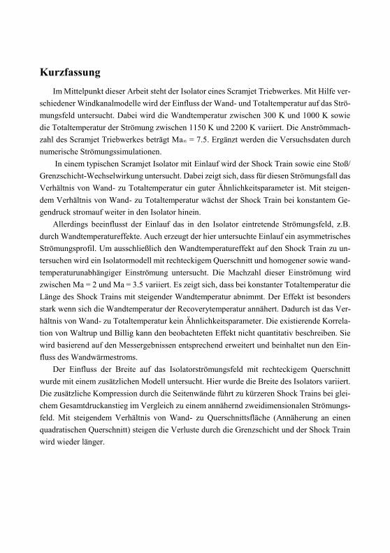
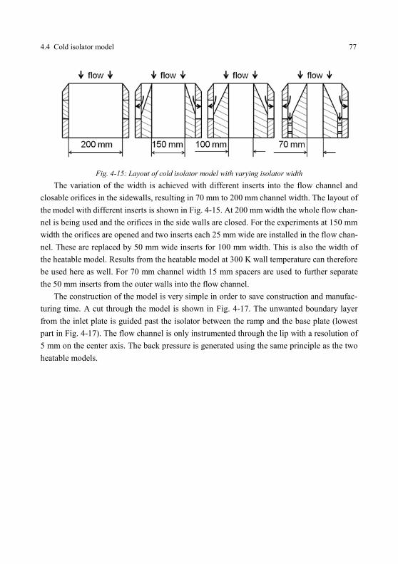
Im Mittelpunkt dieser Arbeit steht der Isolator eines Scramjet Triebwerkes. Mit Hilfe ver-
schiedener Windkanalmodelle wird der Einfluss der Wand- und Totaltemperatur auf das Strö-
mungsfeld untersucht. Dabei wird die Wandtemperatur zwischen 300 K und 1000 K sowie
die Totaltemperatur der Strömung zwischen 1150 K und 2200 K variiert. Die Anströmmach-
zahl des Scramjet Triebwerkes beträgt Ma∞ = 7.5. Ergänzt werden die Versuchsdaten durch
numerische Strömungssimulationen.
In einem typischen Scramjet Isolator mit Einlauf wird der Shock Train sowie eine Stoß/
Grenzschicht-Wechselwirkung untersucht. Dabei zeigt sich, dass für diesen Strömungsfall das
Verhältnis von Wand- zu Totaltemperatur ein guter Ähnlichkeitsparameter ist. Mit steigen-
dem Verhältnis von Wand- zu Totaltemperatur wächst der Shock Train bei konstantem Ge-
gendruck stromauf weiter in den Isolator hinein.
Allerdings beeinflusst der Einlauf das in den Isolator eintretende Strömungsfeld, z.B.
durch Wandtemperatureffekte. Auch erzeugt der hier untersuchte Einlauf ein asymmetrisches
Strömungsprofil. Um ausschließlich den Wandtemperatureffekt auf den Shock Train zu un-
tersuchen wird ein Isolatormodell mit rechteckigem Querschnitt und homogener sowie wand-
temperaturunabhängiger Einströmung untersucht. Die Machzahl dieser Einströmung wird
zwischen Ma = 2 und Ma = 3.5 variiert. Es zeigt sich, dass bei konstanter Totaltemperatur die
Länge des Shock Trains mit steigender Wandtemperatur abnimmt. Der Effekt ist besonders
stark wenn sich die Wandtemperatur der Recoverytemperatur annähert. Dadurch ist das Ver-
hältnis von Wand- zu Totaltemperatur kein Ähnlichkeitsparameter. Die existierende Korrela-
tion von Waltrup und Billig kann den beobachteten Effekt nicht quantitativ beschreiben. Sie
wird basierend auf den Messergebnissen entsprechend erweitert und beinhaltet nun den Ein-
fluss des Wandwärmestroms.
Der Einfluss der Breite auf das Isolatorströmungsfeld mit rechteckigem Querschnitt
wurde mit einem zusätzlichen Modell untersucht. Hier wurde die Breite des Isolators variiert.
Die zusätzliche Kompression durch die Seitenwände führt zu kürzeren Shock Trains bei glei-
chem Gesamtdruckanstieg im Vergleich zu einem annähernd zweidimensionalen Strömungs-
feld. Mit steigendem Verhältnis von Wand- zu Querschnittsfläche (Annäherung an einen
quadratischen Querschnitt) steigen die Verluste durch die Grenzschicht und der Shock Train
wird wieder länger.
I
Contents
Contents ............................................................................................................................ I List of Figures ................................................................................................................ III Tables .............................................................................................................................IX Nomenclature .................................................................................................................XI 1 Introduction............................................................................................................. 1
1.1 Motivation .................................................................................................... 1 1.2 Research training group 1095 ....................................................................... 3
1.2.1 Overview ................................................................................................. 3 1.2.2 Context for presented research ................................................................ 3
2.4.1 Scramjet development in Australia ....................................................... 29 2.4.2 Scramjet development in the USA ........................................................ 30
Fig. 1-1: Specific impulse of air breathing propulsion systems compared to rocket
engines [18] ........................................................................................................... 1 Fig. 1-2: Basic setup of a Scramjet engine ........................................................................... 2 Fig. 2-1: Boundary layer profiles (velocity left and temperature right) calculated with
the Van Driest Technique with varying edge Mach number;
TW = Te = 300 K [35] .......................................................................................... 12 Fig. 2-2: Skin friction coefficient for a laminar and a turbulent boundary layer
obtained with different methods ........................................................................... 18 Fig. 2-3: Stanton number for a laminar and a turbulent boundary layer obtained
with different methods .......................................................................................... 18 Fig. 2-4: Displacement thickness for a laminar and a turbulent boundary layer
obtained with different methods ........................................................................... 19 Fig. 2-5: Momentum thickness for a laminar and a turbulent boundary layer obtained
with different methods .......................................................................................... 19 Fig. 2-6: Sketch of shock wave boundary layer interaction at a compression ramp (left)
and caused by an impinging shock (right) ........................................................... 20 Fig. 2-7: Pressure distribution at a shock boundary layer interaction [66] (left) and
sketch of the complete SWBL (right) .................................................................... 21 Fig. 2-8: Incipient separation pressure as a function of wall temperature ......................... 22 Fig. 2-9: Wall temperature effect on the separation length for three different
correlations .......................................................................................................... 24 Fig. 2-10: Cycle of thermal engines [34] ............................................................................. 25 Fig. 2-11: Wall pressure distributions in combustion chamber without fuel
injection [97] ....................................................................................................... 27 Fig. 2-12: Wall pressure distributions in combustor with fuel injection
(experimental data) [97] ...................................................................................... 27 Fig. 2-13: Combustion pressure rise as a function of total temperature ratio for different
combustor area ratios at Ma3 = 2.5 [5] ............................................................... 28 Fig. 2-14: Plane definition for hypersonic engines ............................................................... 29 Fig. 2-15: Pressure distribution in the HyShort II combustor with and without fuel
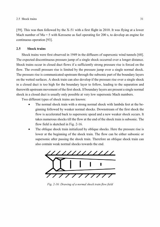
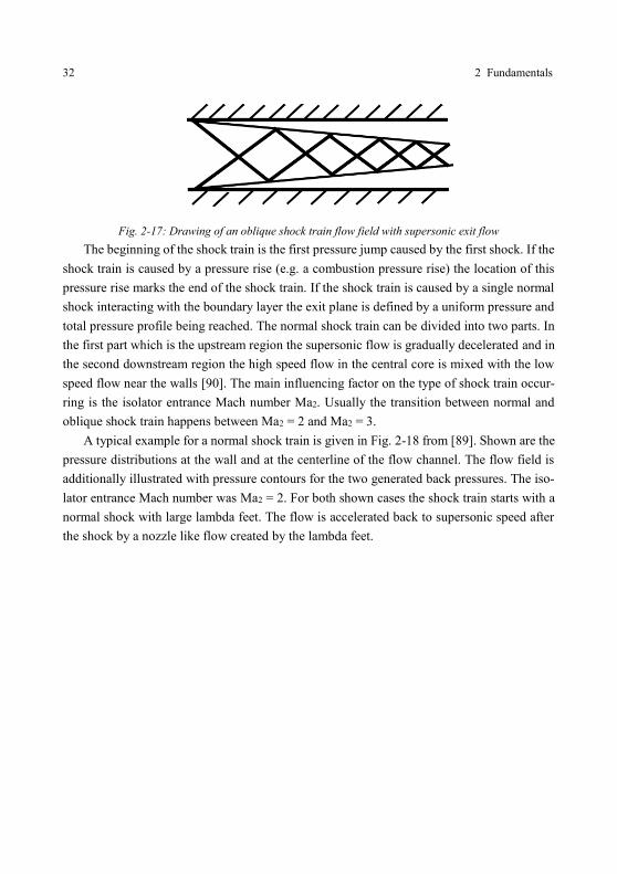
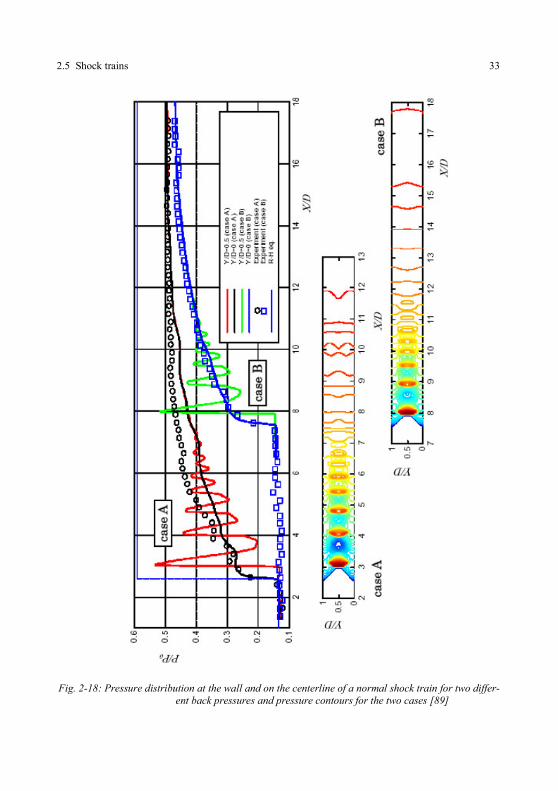
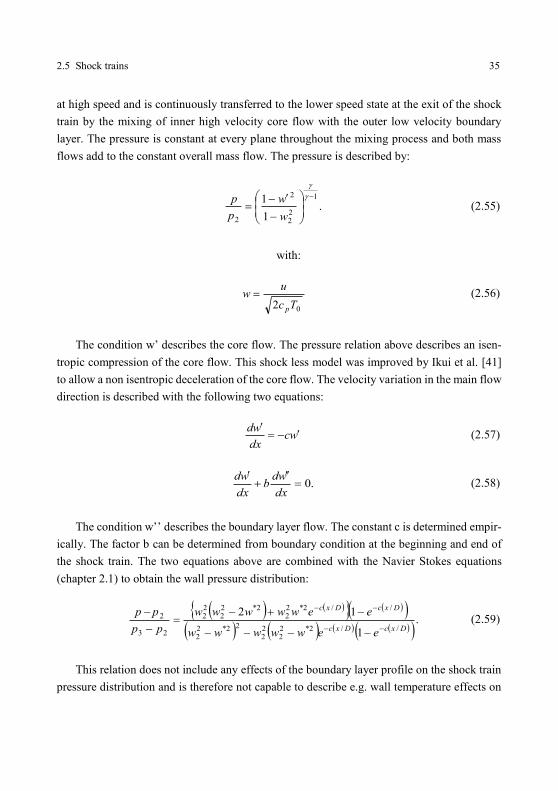
injection[84] ........................................................................................................ 30 Fig. 2-16: Drawing of a normal shock train flow field ......................................................... 31 Fig. 2-17: Drawing of an oblique shock train flow field with supersonic exit flow .............. 32 Fig. 2-18: Pressure distribution at the wall and on the centerline of a normal shock train
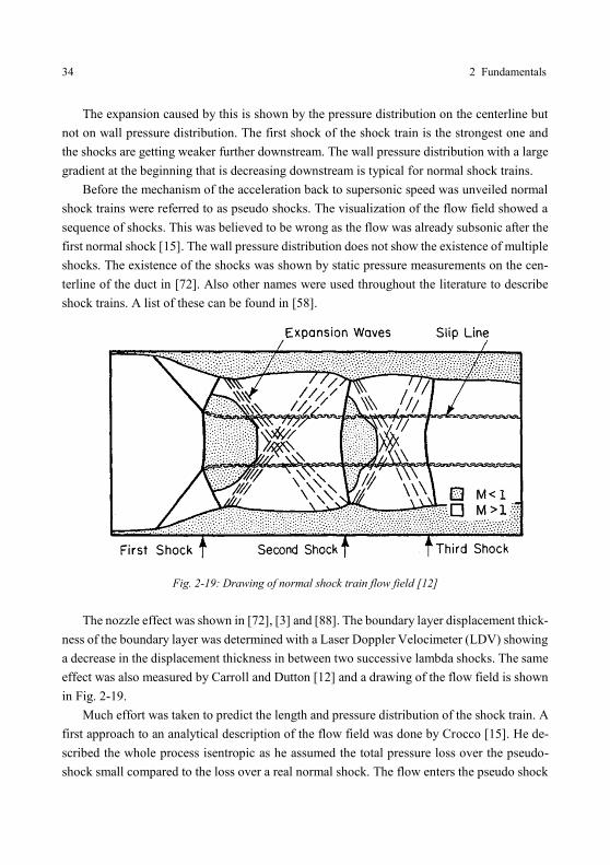
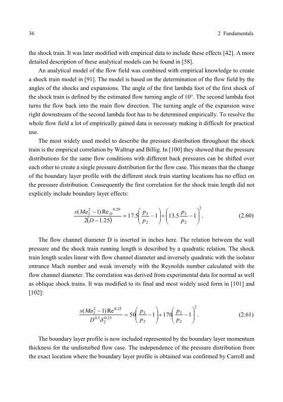
for two different back pressures and pressure contours for the two cases [88] ... 33 Fig. 2-19: Drawing of normal shock train flow field [12] .................................................... 34
IV List of Figures
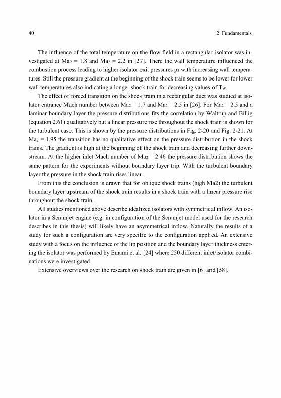
Fig. 2-20: Shock Trains at Ma2 = 1.95 with (bottom) and without forced transition of the
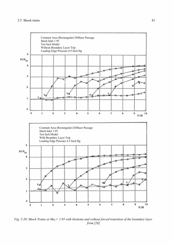
boundary layer from [26] .................................................................................... 41 Fig. 2-21: Shock Trains at Ma2 = 2.46 with (top) and without forced transition of the
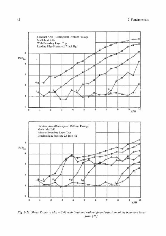
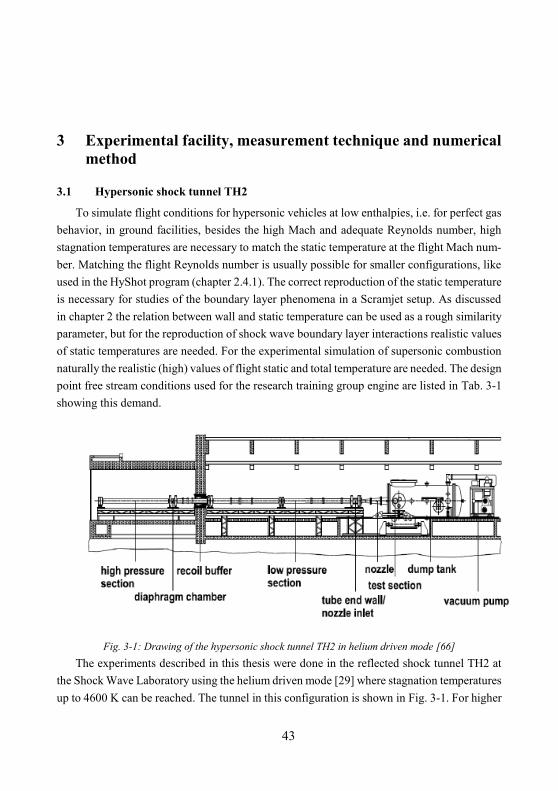
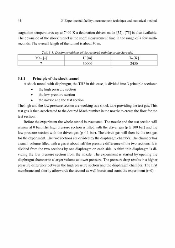
boundary layer from [26] .................................................................................... 42 Fig. 3-1: Drawing of the hypersonic shock tunnel TH2 in helium driven mode [66] .......... 43 Fig. 3-2: Drawing of the shock tube section after bursting of the diaphragms
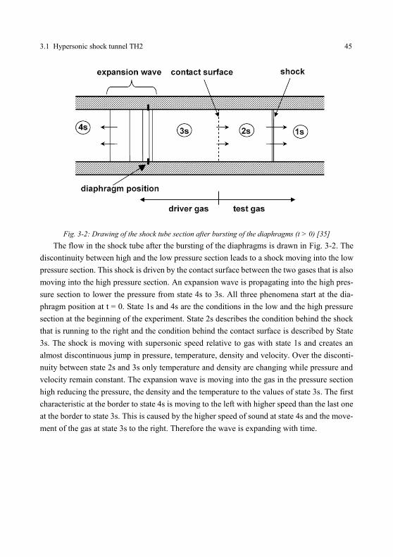
(t > 0) [35] ........................................................................................................... 45 Fig. 3-3: x-t diagram of the shock tube process in the TH2 facility in helium driven
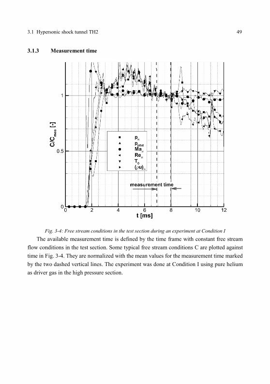
mode [35] ............................................................................................................ 46 Fig. 3-4: Free stream conditions in the test section during an experiment at Condition I .. 49 Fig. 3-5: Free stream conditions in the test section during an experiment at Condition I
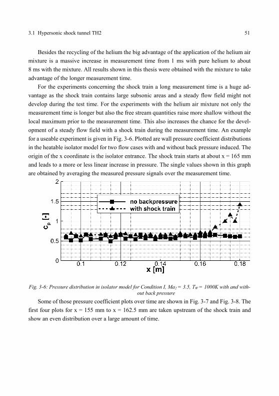
with a helium air mixture ..................................................................................... 50 Fig. 3-6: Pressure distribution in isolator model for Condition I, Ma2 = 3.5,
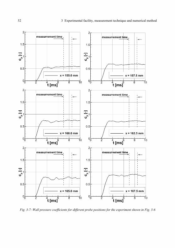
TW = 1000K with and without back pressure ....................................................... 51 Fig. 3-7: Wall pressure coefficients for different probe positions for the experiment
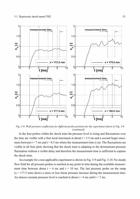
shown in Fig. 3-6 ................................................................................................. 52 Fig. 3-8: Wall pressure coefficients for different probe positions for the experiment
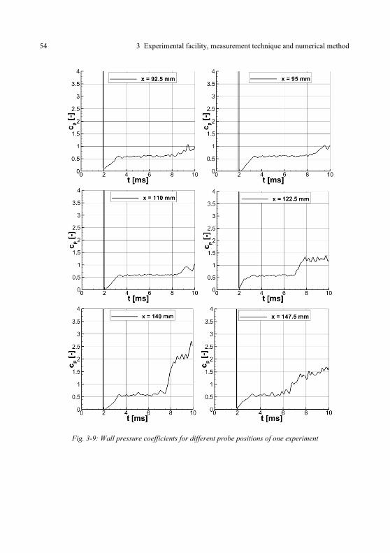
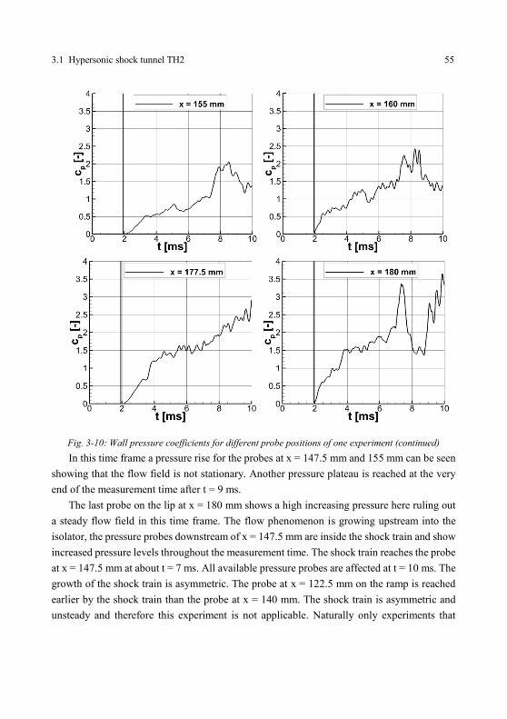
shown in Fig. 3-6 (continued) .............................................................................. 53 Fig. 3-9: Wall pressure coefficients for different probe positions of one experiment ......... 54 Fig. 3-10: Wall pressure coefficients for different probe positions of one experiment
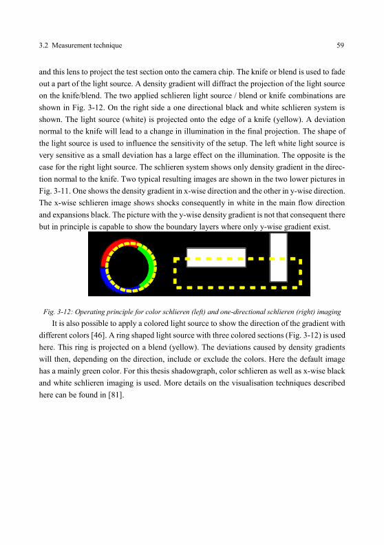
image for the same flow field. .............................................................................. 58 Fig. 3-12: Operating principle for color schlieren (left) and one-directional schlieren
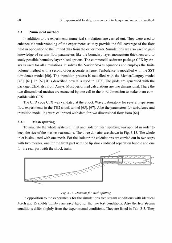
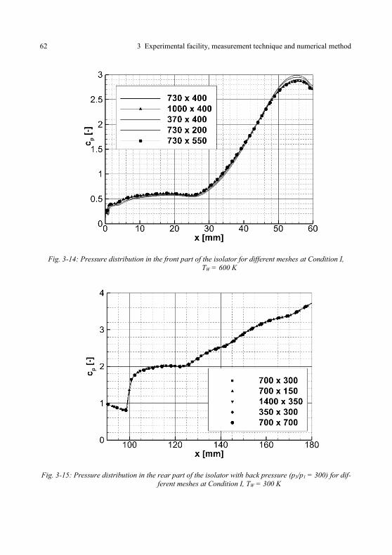
(right) imaging ..................................................................................................... 59 Fig. 3-13: Domains for mesh splitting .................................................................................. 60 Fig. 3-14: Pressure distribution in the front part of the isolator for different meshes .......... 62 Fig. 3-15: Pressure distribution in the rear part of the isolator with back pressure for
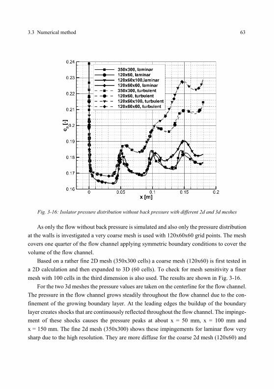
different meshes ................................................................................................... 62 Fig. 3-16: Isolator pressure distribution without back pressure with different 2d and 3d
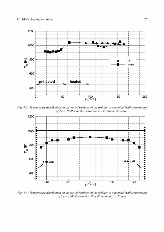
meshes .................................................................................................................. 63 Fig. 4-1: Cut through the cooling section [66] ................................................................... 65 Fig. 4-2: Temperature distribution on the wetted surfaces of the isolator at a nominal
wall temperature of TW = 1000 K on the centerline in streamwise direction ....... 67 Fig. 4-3: Temperature distribution on the wetted surfaces of the isolator at a nominal
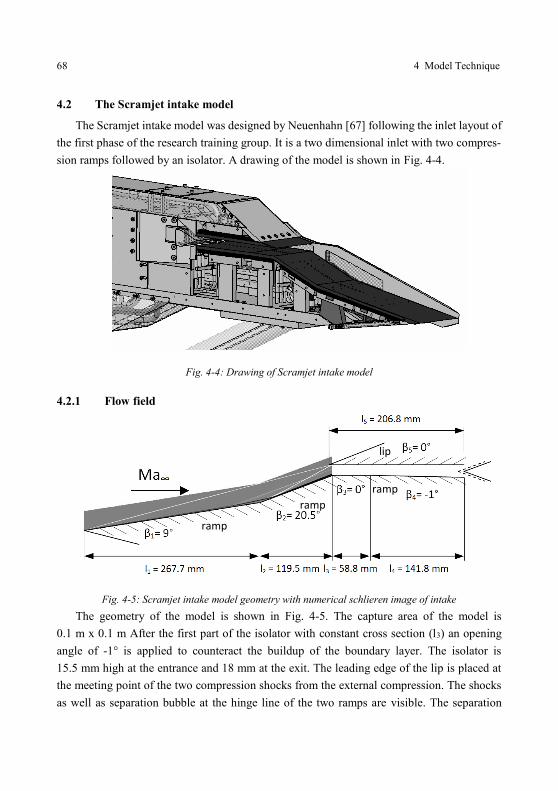
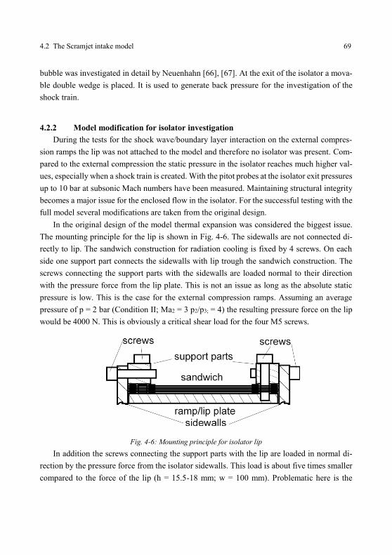
wall temperature of TW = 1000 K normal to flow direction at x = 25 mm ........... 67 Fig. 4-4: Drawing of Scramjet intake model ....................................................................... 68 Fig. 4-5: Scramjet intake model geometry with numerical schlieren image of intake......... 68
List of Figures V
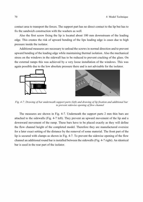
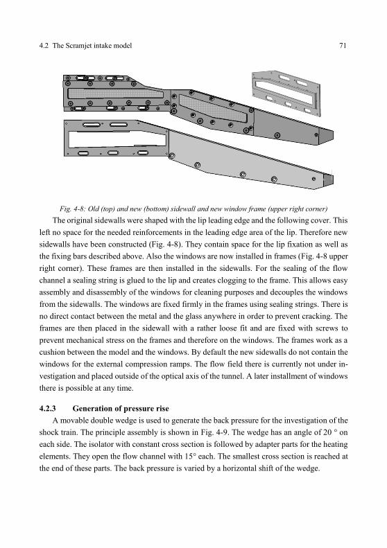
Fig. 4-6: Mounting principle for isolator lip ...................................................................... 69 Fig. 4-7: Drawing of bar underneath support parts (left) and drawing of lip fixation
and additional bar to prevent sidewise opening of flow channel ......................... 70 Fig. 4-8: Old (top) and new (bottom) sidewall and new window frame
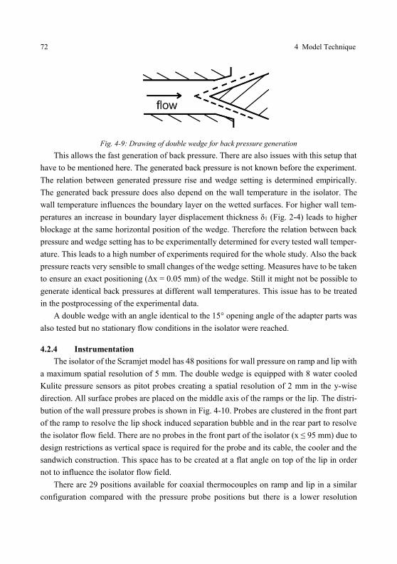
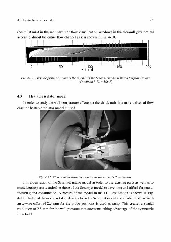
(upper right corner) ............................................................................................. 71 Fig. 4-9: Drawing of double wedge for back pressure generation ..................................... 72 Fig. 4-10: Pressure probe positions in the isolator of the Scramjet model with
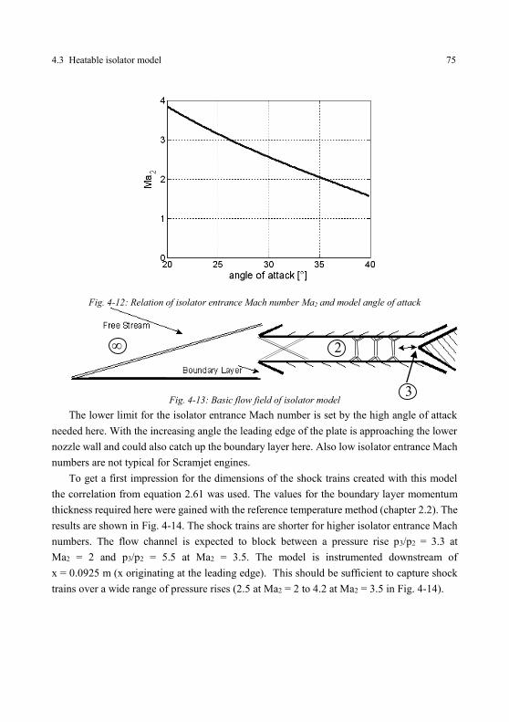
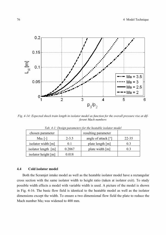
shadowgraph image (Cond. I, TW = 300 K) ......................................................... 73 Fig. 4-11: Picture of the heatable isolator model in the TH2 test section ............................ 73 Fig. 4-12: Relation of isolator entrance Mach number Ma2 and model angle of attack ....... 75 Fig. 4-13: Basic flow field of isolator model ........................................................................ 75 Fig. 4-14: Expected shock train length in isolator model as function for the overall
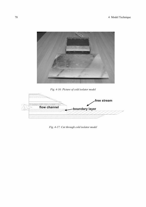
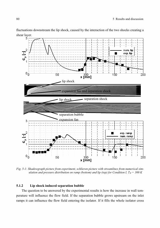
pressure rise at different Mach numbers .............................................................. 76 Fig. 4-15: Layout of cold isolator model with varying isolator width .................................. 77 Fig. 4-16: Picture of cold isolator model ............................................................................. 78 Fig. 4-17: Cut through cold isolator model .......................................................................... 78 Fig. 5-1: Shadowgraph picture from experiment, schlieren picture with streamlines
from numerical simulation and pressure distribution on ramp (bottom) and
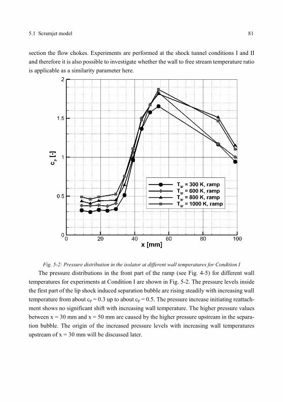
lip (top) for Condition I, TW = 300 K .................................................................. 80 Fig. 5-2: Pressure distribution in the isolator at different wall temperatures for
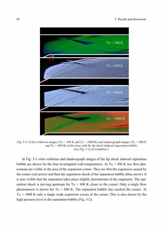
Condition I ........................................................................................................... 81 Fig. 5-3: Color schlieren images (TW = 300 K and TW = 1000 K) and shadowgraph
images (TW = 600 K and TW = 800 K) of lip shock induced separation bubble
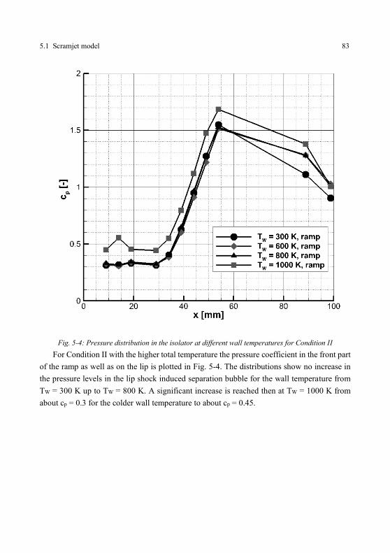
at Condition I ....................................................................................................... 82 Fig. 5-4: Pressure distribution in the isolator at different wall temperatures for
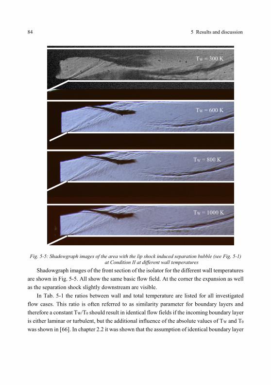
Condition II .......................................................................................................... 83 Fig. 5-5: Shadowgraph images of lip shock induced separation bubble at Condition II
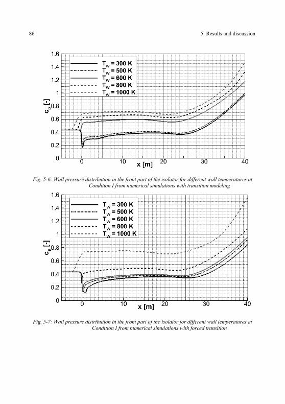
at different wall temperatures .............................................................................. 84 Fig. 5-6: Wall pressure distribution in the front part of the isolator for different wall
temperatures at Condition I from numerical simulations with transition
modeling .............................................................................................................. 86 Fig. 5-7: Wall pressure distribution in the front part of the isolator for different wall
temperatures at Condition I from numerical simulations with forced
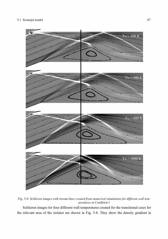
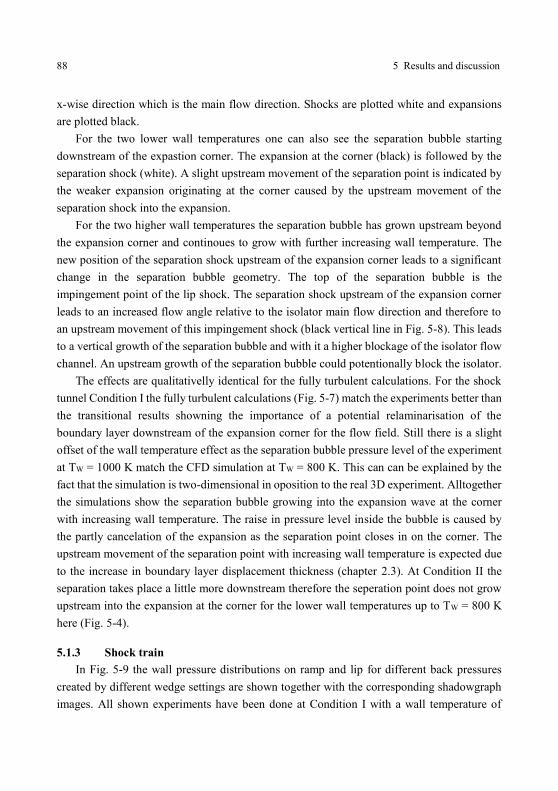
transition .............................................................................................................. 86 Fig. 5-8: Schlieren images with stream lines created from numerical simulations for
different wall temperatures at Condition I ........................................................... 87
VI List of Figures
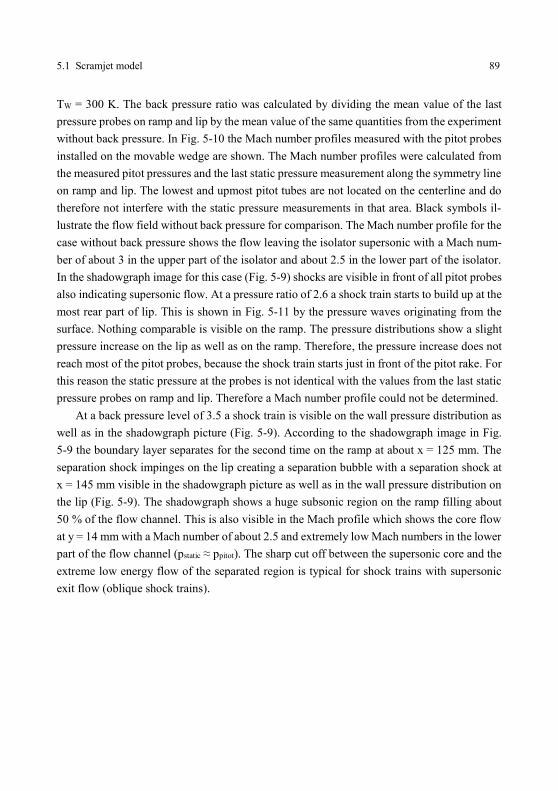
Fig. 5-9: Pressure distributions on ramp (bottom) and lip (top) for different pressure
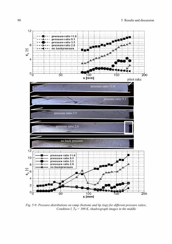
ratios, Condition I, TW = 300 K, shadowgraph images in the middle .................. 90 Fig. 5-10: Mach number profiles at isolator exit (pitot rake position) for different back
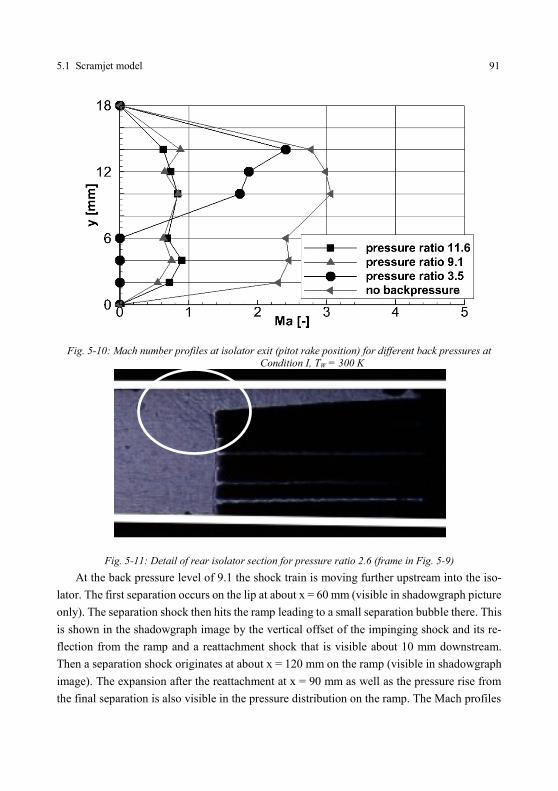
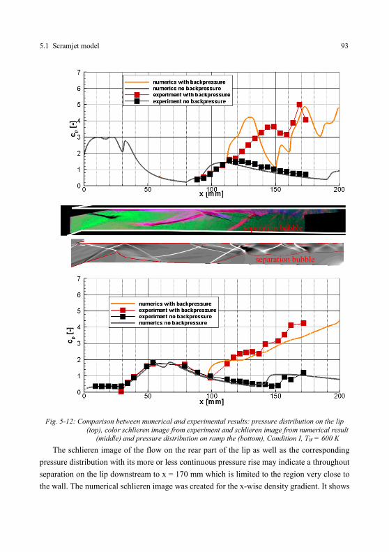
pressures at Condition I, TW = 300 K .................................................................. 91 Fig. 5-11: Detail of rear isolator section for pressure ratio 2.6 (frame in Fig. 5-9) ............ 91 Fig. 5-12: Comparison between numerical and experimental results: pressure
distribution on the lip (top), color schlieren image from experiment and
schlieren image from numerical result (middle) and pressure distribution on
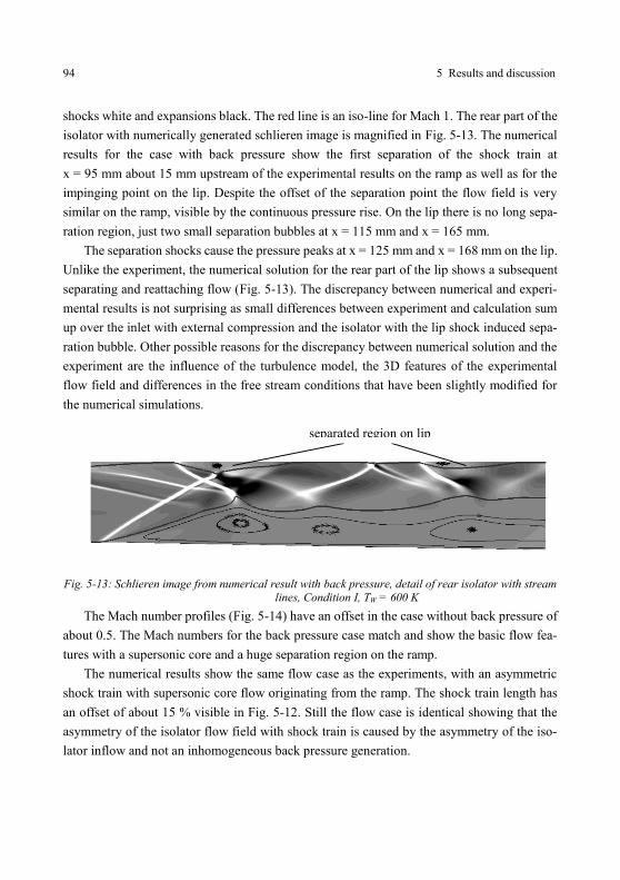
ramp the (bottom), Condition I, TW = 600 K ........................................................ 93 Fig. 5-13: Schlieren image from numerical result with back pressure, detail of rear
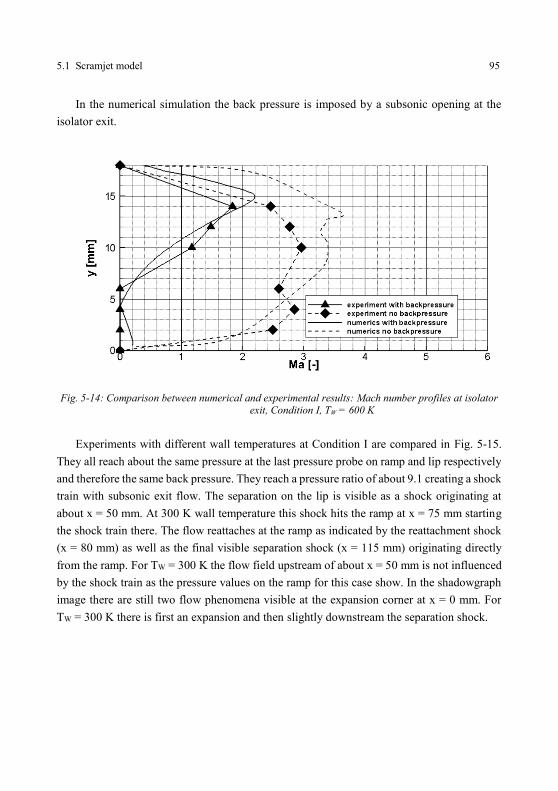
isolator with stream lines, Condition I, TW = 600 K ............................................ 94 Fig. 5-14: Comparison between numerical and experimental results: Mach number
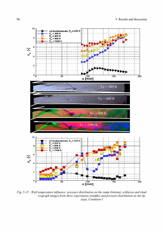
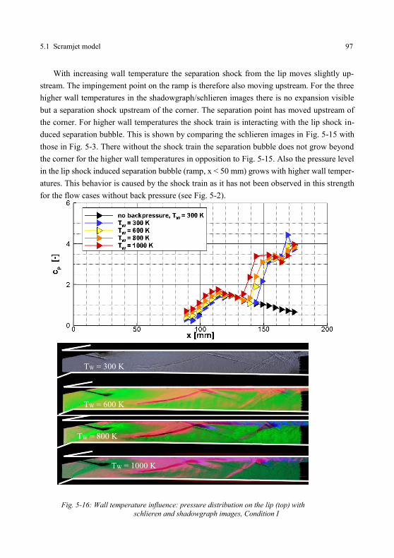
profiles at isolator exit, Condition I, TW = 600 K ................................................ 95 Fig. 5-15 : Wall temperature influence: pressure distribution on the ramp (bottom),
schlieren and shadowgraph images from these experiments (middle) and
pressure distribution on the lip (top), Condition I ............................................... 96 Fig. 5-16: Wall temperature influence: pressure distribution on the lip (top) with
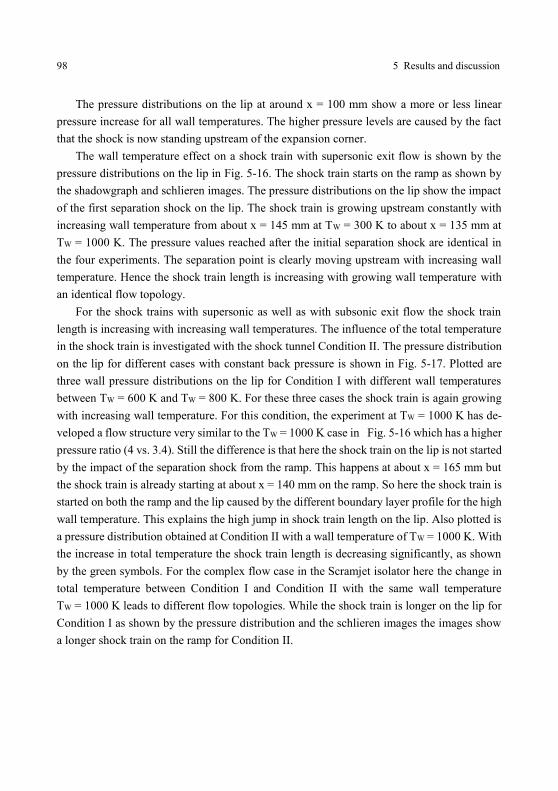
schlieren and shadowgraph images, Condition I ................................................. 97 Fig. 5-17: Wall and total temperature influence: pressure distribution on the lip (top)
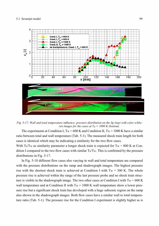
with color schlieren images for the cases at TW = 1000 K (bottom) .................... 99 Fig. 5-18: Wall and total temperature influence: pressure distribution on the ramp (top)
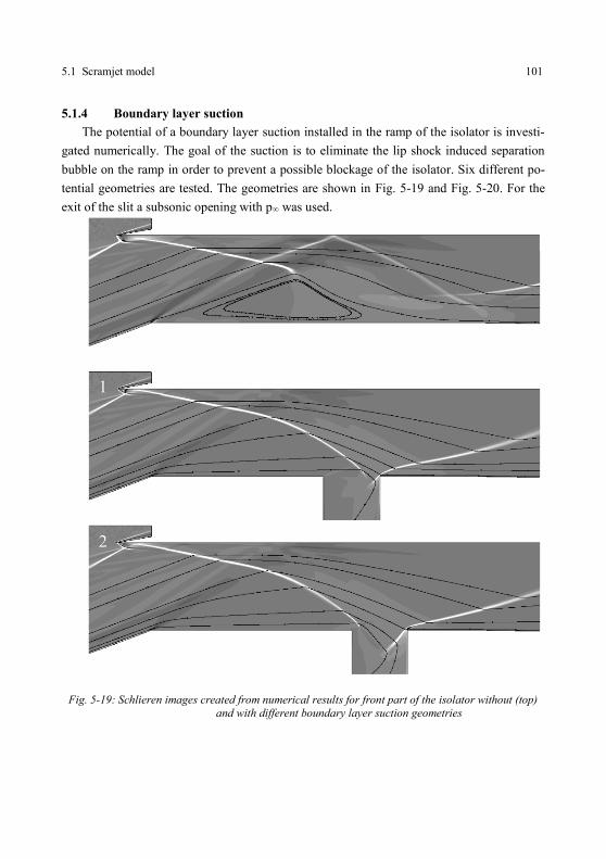
with shadowgraph images (bottom) ................................................................... 100 Fig. 5-19: Schlieren images created from numerical results for front part of the isolator
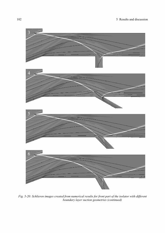
without (top) and with different boundary layer suction geometries .................. 101 Fig. 5-20: Schlieren images created from numerical results for front part of the isolator
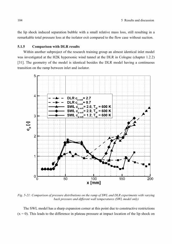
with different boundary layer suction geometries (continued) ........................... 102 Fig. 5-21: Comparison of pressure distributions on the ramp of SWL and DLR
experiments with varying back pressure and different wall temperatures
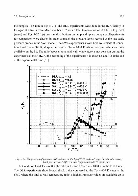
(SWL model only)............................................................................................... 104 Fig. 5-22: Comparison of pressure distributions on the lip of SWL and DLR
experiments with varying back pressure and different wall temperatures
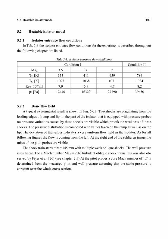
(SWL model only)............................................................................................... 105 Fig. 5-23: Schlieren image (bottom) and wall pressure distribution (top) at Condition I,
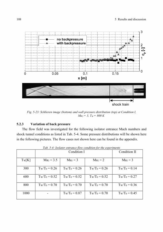
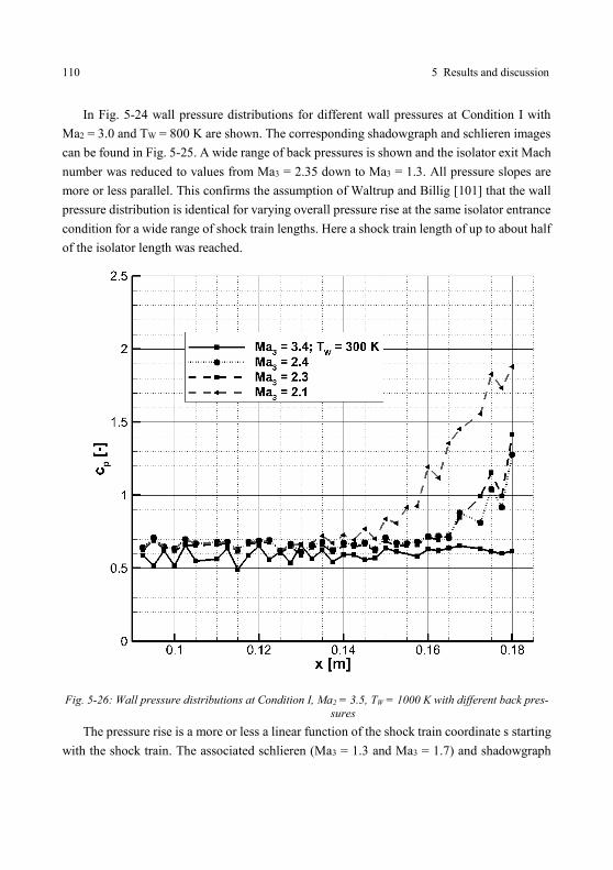
Ma2 = 3, TW = 800 K ......................................................................................... 108 Fig. 5-24: Wall pressure distributions at Condition I, Ma2 = 3.0, TW = 800 K with
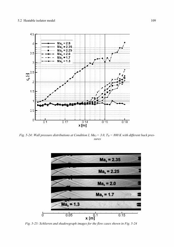
different back pressures ..................................................................................... 109 Fig. 5-25: Schlieren and shadowgraph images for the flow cases shown in Fig. 5-24 ....... 109
List of Figures VII
Fig. 5-26: Wall pressure distributions at Condition I, Ma2 = 3.5, TW = 1000 K with
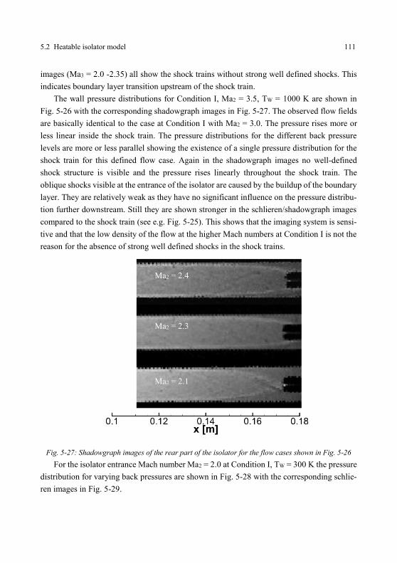
different back pressures ..................................................................................... 110 Fig. 5-27: Shadowgraph images of the rear part of the isolator for the flow cases shown
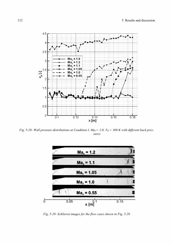
in Fig. 5-26 ........................................................................................................ 111 Fig. 5-28: Wall pressure distributions at Condition I, Ma2 = 2.0, TW = 300 K with
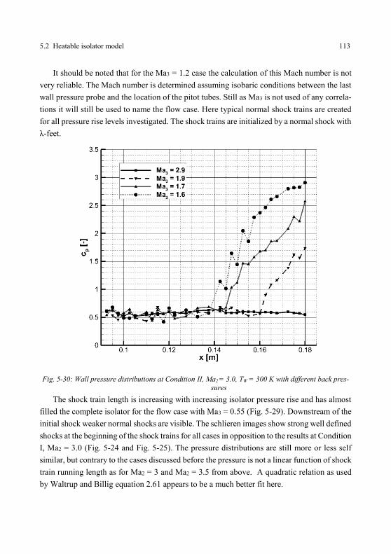
different back pressures ..................................................................................... 112 Fig. 5-29: Schlieren images for the flow cases shown in Fig. 5-28 .................................... 112 Fig. 5-30: Wall pressure distributions at Condition II, Ma2 = 3.0, TW = 300 K with
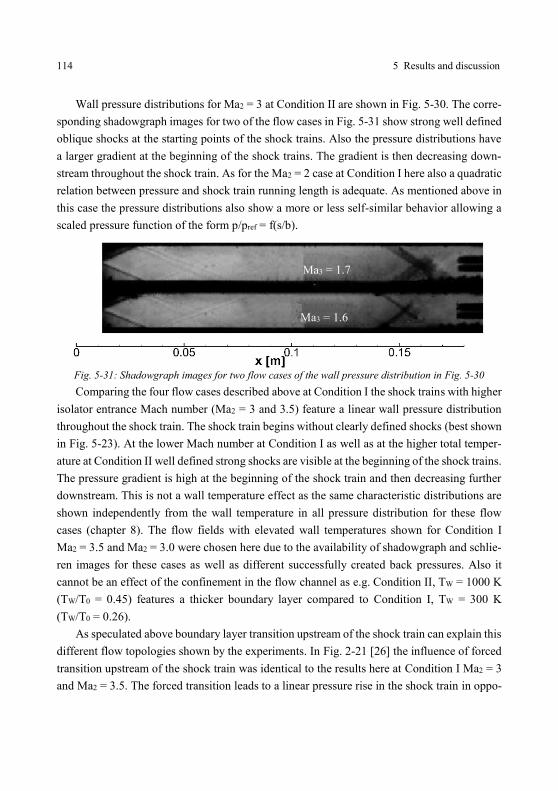
different back pressures ..................................................................................... 113 Fig. 5-31: Shadowgraph images for two flow cases of the wall pressure distribution in
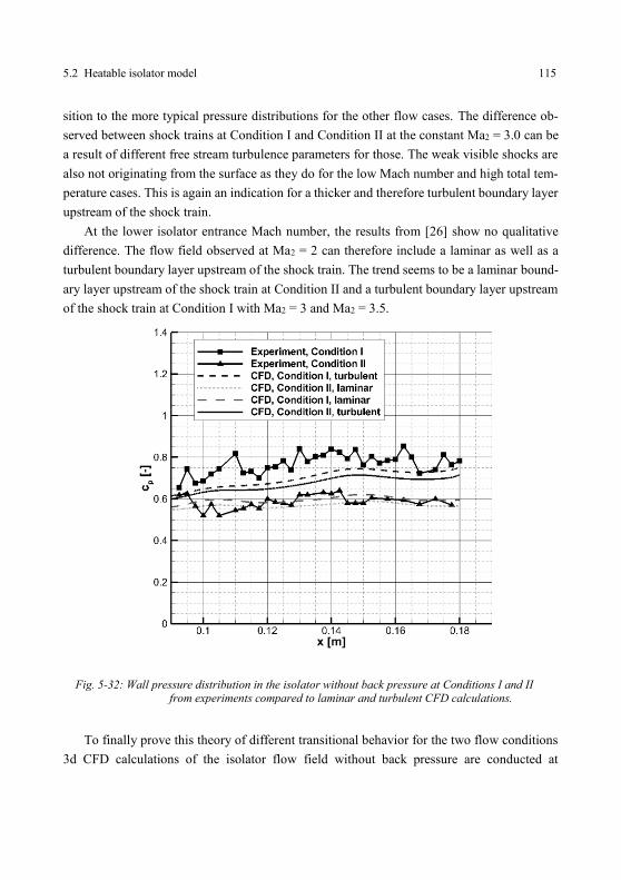
Fig. 5-30 ............................................................................................................ 114 Fig. 5-32: Wall pressure distribution in the isolator without back pressure at
Conditions I and II from experiments compared to laminar and turbulent
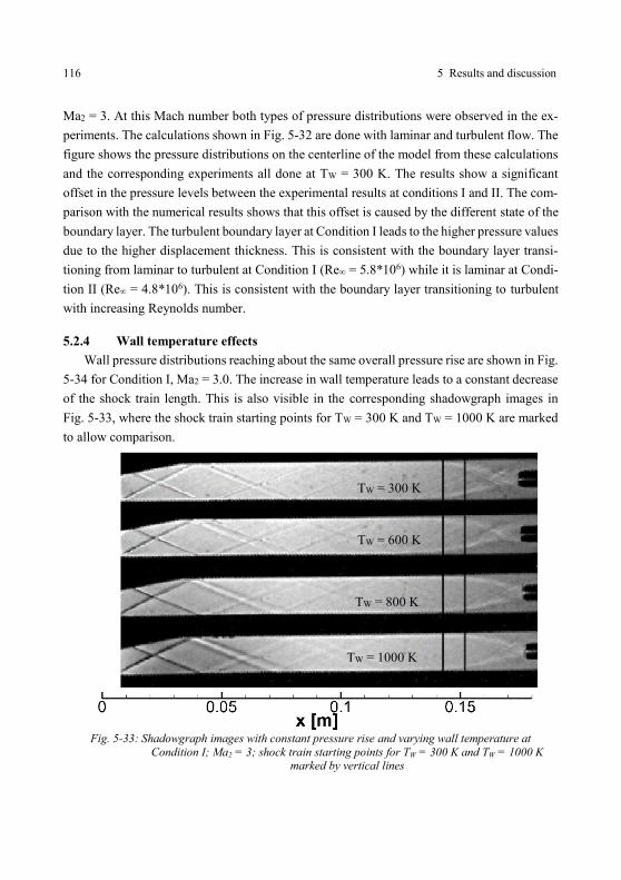
CFD calculations. .............................................................................................. 115 Fig. 5-33: Shadowgraph images with constant pressure rise and varying wall
temperature at Condition I; Ma2 = 3; shock train starting points for
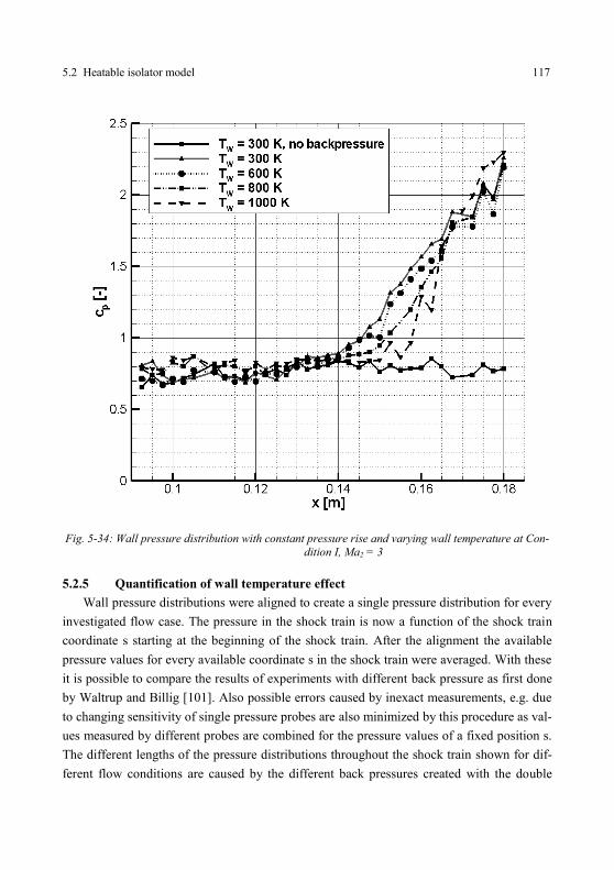
TW = 300 K and TW = 1000 K marked by vertical lines ..................................... 116 Fig. 5-34: Wall pressure distribution with constant pressure rise and varying wall
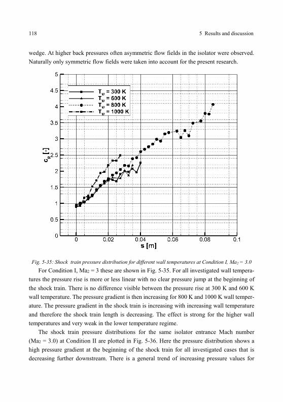
temperature at Condition I, Ma2 = 3 ................................................................. 117 Fig. 5-35: Shock train pressure distribution for different wall temperatures at
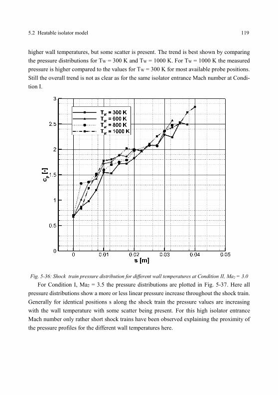
Condition I, Ma2 = 3.0 ....................................................................................... 118 Fig. 5-36: Shock train pressure distribution for different wall temperatures at
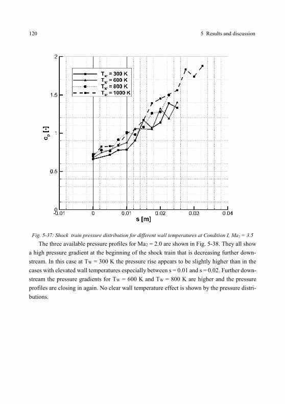
Condition II, Ma2 = 3.0...................................................................................... 119 Fig. 5-37: Shock train pressure distribution for different wall temperatures at
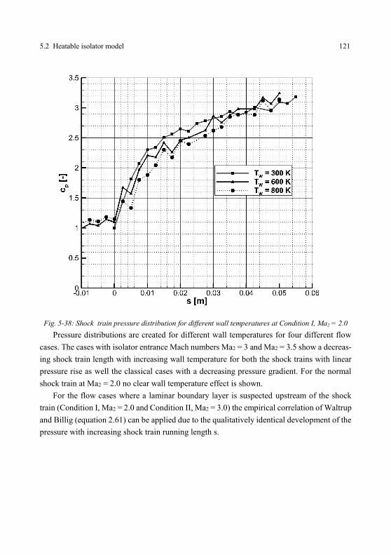
Condition I, Ma2 = 3.5 ....................................................................................... 120 Fig. 5-38: Shock train pressure distribution for different wall temperatures at
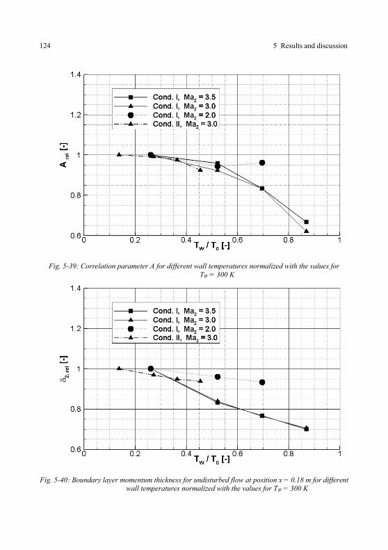
Condition I, Ma2 = 2.0 ....................................................................................... 121 Fig. 5-39: Correlation parameter A for different wall temperatures normalized with the
values for TW = 300 K ........................................................................................ 124 Fig. 5-40: Boundary layer momentum thickness at position x = 0.18 m for different wall
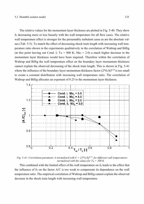
temperatures normalized with the values for TW = 300 K .................................. 124 Fig. 5-41: Correlation parameter A normalized with C = [2*δ2/h]0.25 for different wall
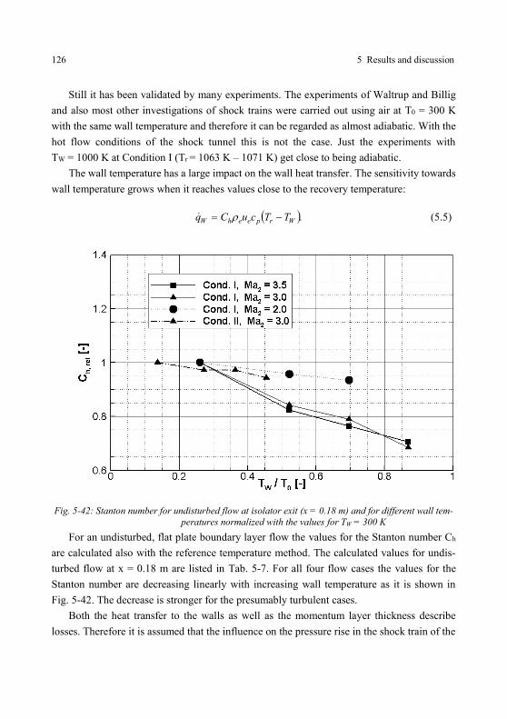
temperatures normalized with the values for TW = 300 K .................................. 125 Fig. 5-42: Stanton number for undisturbed flow at isolator exit (x = 0.18 m) and for
different wall temperatures normalized with the values for TW = 300 K............ 126
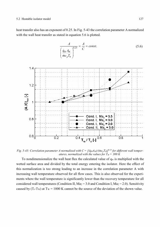
Fig. 5-43: Correlation parameter A normalized with C = [(q.
WAW)/(m.cpT0)]0.25 for
different wall temperatures, normalized with the values for TW = 300 K........... 127
VIII List of Figures
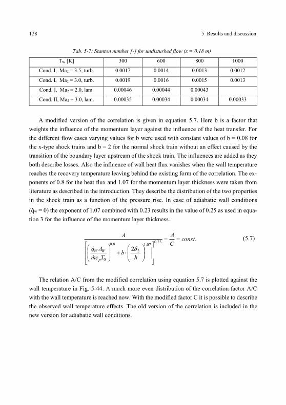
Fig. 5-44: Correlation parameter A normalized with C from equation 5.7 for different
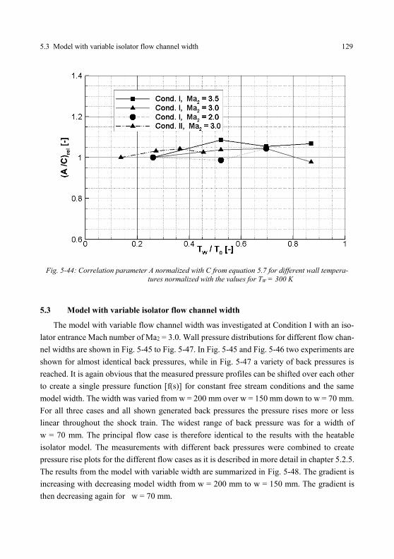
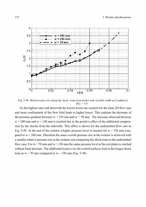
wall temperatures normalized with the values for TW = 300 K .......................... 129 Fig. 5-45: Pressure distributions for 200 mm flow channel width ...................................... 130 Fig. 5-46: Pressure distributions for 150 mm flow channel width ...................................... 130 Fig. 5-47: Pressure distributions for 70 mm flow channel width ........................................ 131 Fig. 5-48: Wall pressure rise along the shock train from model with variable width at
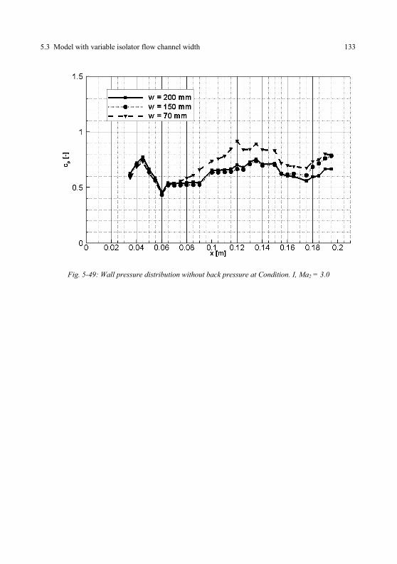
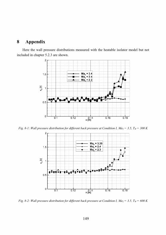
Condition I, Ma2 = 3.0 ....................................................................................... 132 Fig. 5-49: Wall pressure distribution without back pressure at Condition. I, Ma2 = 3.0 ... 133 Fig. 8-1: Wall pressure distribution for different back pressure at Condition I,
Ma2 = 3.5, TW = 300 K ...................................................................................... 149 Fig. 8-2: Wall pressure distribution for different back pressure at Condition I,
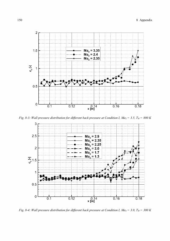
Ma2 = 3.5, TW = 600 K ...................................................................................... 149 Fig. 8-3: Wall pressure distribution for different back pressure at Condition I,
Ma2 = 3.5, TW = 800 K ...................................................................................... 150 Fig. 8-4: Wall pressure distribution for different back pressure at Condition I,
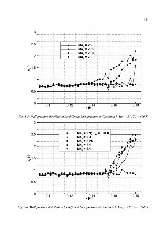
Ma2 = 3.0, TW = 300 K ...................................................................................... 150 Fig. 8-5: Wall pressure distribution for different back pressure at Condition I,
Ma2 = 3.0, TW = 600 K ...................................................................................... 151 Fig. 8-6: Wall pressure distribution for different back pressure at Condition I,
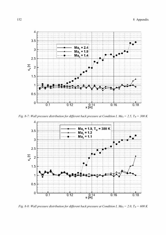
Ma2 = 3.0, TW = 1000 K .................................................................................... 151 Fig. 8-7: Wall pressure distribution for different back pressure at Condition I,
Ma2 = 2.5, TW = 300 K ...................................................................................... 152 Fig. 8-8: Wall pressure distribution for different back pressure at Condition I,
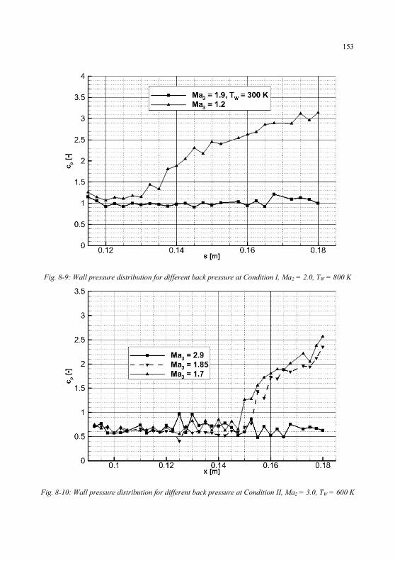
Ma2 = 2.0, TW = 600 K ...................................................................................... 152 Fig. 8-9: Wall pressure distribution for different back pressure at Condition I,
Ma2 = 2.0, TW = 800 K ...................................................................................... 153 Fig. 8-10: Wall pressure distribution for different back pressure at Condition II,
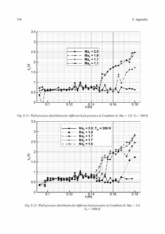
Ma2 = 3.0, TW = 600 K ...................................................................................... 153 Fig. 8-11: Wall pressure distribution for different back pressure at Condition II,
Ma2 = 3.0, TW = 800 K ...................................................................................... 154 Fig. 8-12: Wall pressure distribution for different back pressure at Condition II,
Ma2 = 3.0, TW = 1000 K .................................................................................... 154
IX
Tables
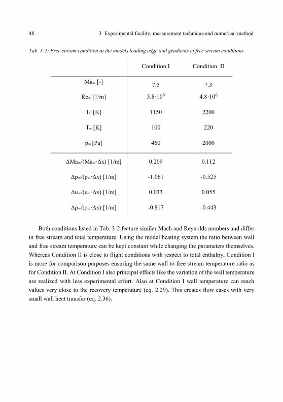
Tab. 2-1: Flow condition for boundary layer calculation ..................................................... 17 Tab. 3-1: Design conditions of the research training group Scramjet .................................. 44 Tab. 3-2: Free stream condition at the models leading edge and gradients of free stream
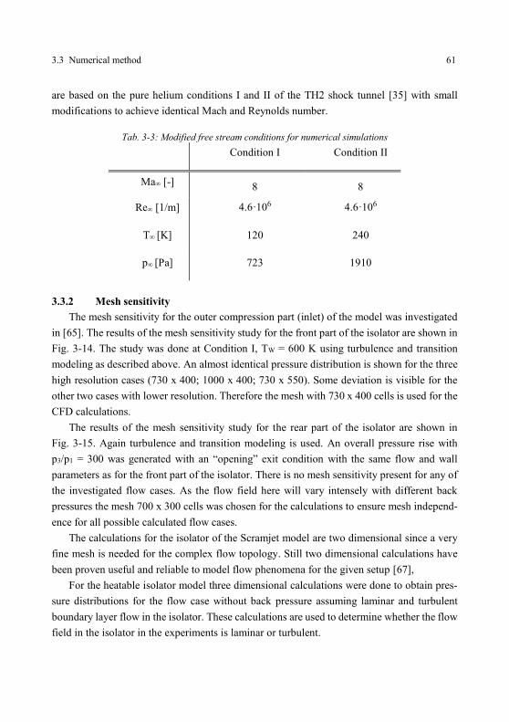
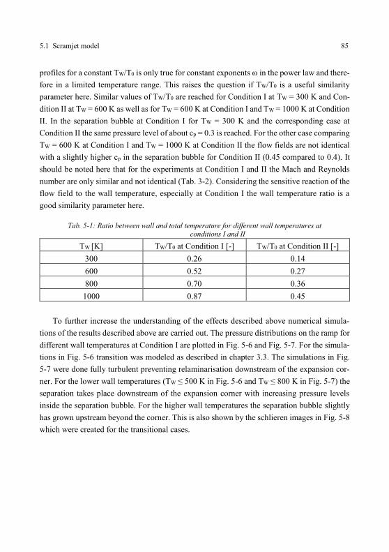
conditions .............................................................................................................. 48 Tab. 3-3: Modified free stream conditions for numerical simulations .................................. 61 Tab. 4-1: Design parameters for the heatable isolator model .............................................. 76 Tab. 5-1: Ratio between wall and total temperature for different wall temperatures at
conditions I and II ................................................................................................. 85 Tab. 5-2: Relative bleed mass flow and relative total pressure level at exit for the
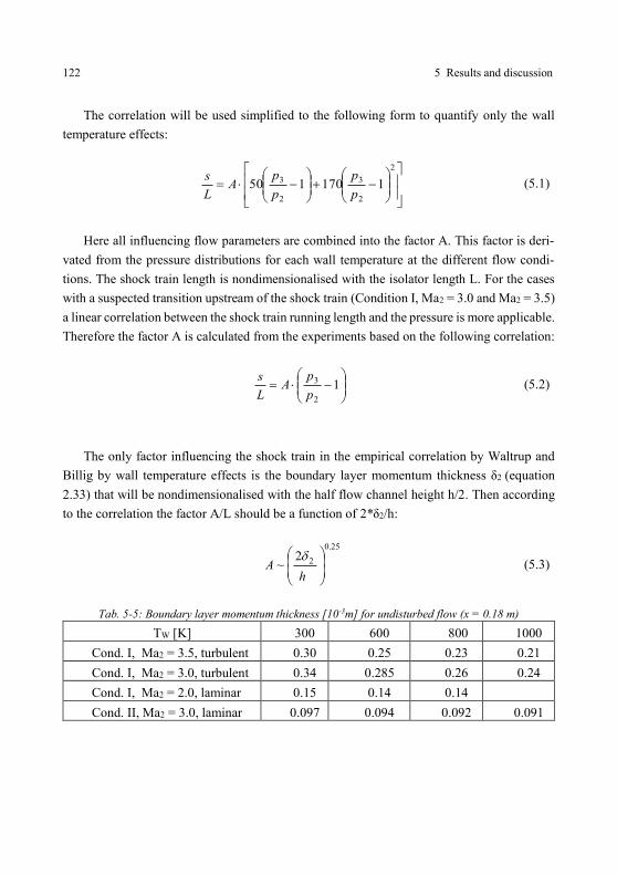
different bleed configurations ............................................................................. 103 Tab. 5-3: Isolator entrance flow conditions ........................................................................ 107 Tab. 5-4: Isolator entrance flow condition for the experiments .......................................... 108 Tab. 5-5: Boundary layer momentum thickness [10-3m] for undisturbed flow
(x = 0.18 m)......................................................................................................... 122 Tab. 5-6: Parameter A for the investigated flow cases calculated from the pressure
distributions ........................................................................................................ 123 Tab. 5-7: Stanton number [-] for undisturbed flow (x = 0.18 m) ........................................ 128
XI
Nomenclature
A amplification factor [-], correlation parameter [-]
A* critical area [m2]
C Sutherland factor [kg/(m s K0.5)], measured free stream quantity,
wall temperature influence factor [-]
CH Stanton number [-]
D flow channel diameter [m]
H altitude [m], flow channel height [m]
L characteristic length [m]
LMess pressure pipe length [m]
M molecular weight [g/Mol]
Ma Mach number [-]
Pr Prandl number [-]
R specific gas constant [J/(kg K)]
Re unit Reynolds number [1/m]
Re,x Reynolds number [-]
S Sutherland temperature [K]
T temperature [K]
TR recovery temperature [K]
T0 total temperature [K]
V volume [m3]
X probe signal [V]
a1-4 thermocouple calibration factors [K/V]
b weighting factor [-]
c specific thermal capacity [J/(kg*K)]
cf skin friction coefficient [-]
cp pressure coefficient [-]
cµ power law factor [kg/(m s K(1-ω))]
di pressure pipe inner diameter [m]
e internal energy [J/kg]
fe eigenfrequency [Hz]
h flow channel height [m]
k thermal conductivity [W/m*K]
XII Nomenclature
l length [m]
p pressure [Pa]
p0 total pressure [Pa]
pp pitot pressure [Pa]
q dynamic pressure [Pa], q = 0.5ρu2
q. heat transfer [W/m2]
r recovery factor [-]
s coordinate in x-wise direction starting at the shock train [m]
t time [s]
t95 time for throttle device to achieve 95% of the mass flow [s]
tr response time [s]
u velocity [m/s], x-wise velocity [m/s]
v y-wise velocity[m/s]
w flow channel width [m], z-wise velocity [m/s]
x coordinate in main flow direction starting at isolator entrance [m]
y coordinate normal to ramp plane starting at ramp [m]
β ramp angle [°]
γ ratio of the specific heats
δ boundary layer thickness [m]
δ1 boundary layer displacement thickness [m]
δ2 boundary layer momentum thickness [m]
ρ density [kg/m3]
τ shear stress [N/m2]
τs time constant for t95 [s]
µ dynamic viscosity [kg/(m s)]
ω power law exponent [-]
Suffix
∞ free stream condition
0 stagnation condition
2 isolator entrance condition
3 isolator exit condition
1s low pressure section of shock tube before experiment
2s downstream of shock in low pressure section of shock tube
Nomenclature XIII
3s downstream of contact surface in low pressure section of shock tube
4s high pressure section of shock tube before experiment
e edge condition
C cavity in front of pressure probe
L shock impingement location for inviscid flow
Mea during measurement time
p plenum
ref reference condition
td throttle device
W wall condition
x in x-wise direction
y in y-wise direction
Superfix
* critical condition (Ma = 1)
1
1 Introduction
1.1 Motivation
Today rocket propulsion systems such as the Ariane V and the Sojus rocket are used as
space transportation systems. A rocket engine carries its own fuel and oxidizer and works
independent from the flight Mach number and atmospheric pressure (except the supersonic
nozzle) but the maximum specific impulse is very limited. The payload ratio of these systems
is in the range of low single digit percentage numbers. None of the in use systems is reusable
and all require staging. For a drastic reduction of the costs of transport to space reusable sys-
tems ideally without staging are needed. To compensate for the higher structural weight of
these propulsion systems caused by the structural mass of the reentry system and the addi-
tional mass due to the lack of staging systems with a higher specific impulse are needed. This
can be achieved by using air breathing propulsion systems.
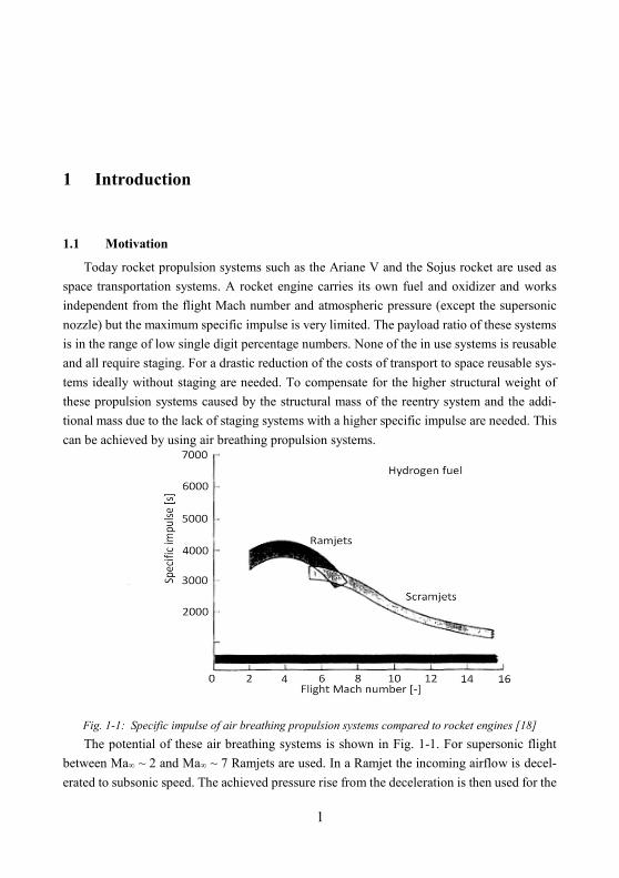
Fig. 1-1: Specific impulse of air breathing propulsion systems compared to rocket engines [18]
The potential of these air breathing systems is shown in Fig. 1-1. For supersonic flight
between Ma∞ ~ 2 and Ma∞ ~ 7 Ramjets are used. In a Ramjet the incoming airflow is decel-
erated to subsonic speed. The achieved pressure rise from the deceleration is then used for the
2 1 Introduction
combustion cycle. With increasing Mach number the total pressure loss created by the shocks
in the compression process is increasing. From about Ma∞ = 6 Scramjets offer a higher possi-
ble specific impulse. In a Scramjet (Supersonic combustion Ramjet) the air is only decelerated
to lower supersonic velocities (about 1/3 of Ma∞ [33]). This creates lower total pressure losses
but higher drag on the wetted walls due to the higher Mach number in the combustion chamber
as well as the longer flow path needed to achieve mixing and combustion.
Also both Ramjet and Scramjet are not operational below a certain Mach number as they
require the flight velocity to create compression. In an operational system they are also very
likely to be combined (dual-mode operation) in a single flow path to enable operation over a
wide Mach number range. The overall thrust created by Scramjet systems is the difference
between thrust created by the system and the drag, which are both large numbers. Small
changes in one of the two have a large impact on the overall system performance. Therefore
a good understanding of the exact performance of every component in the system is needed.
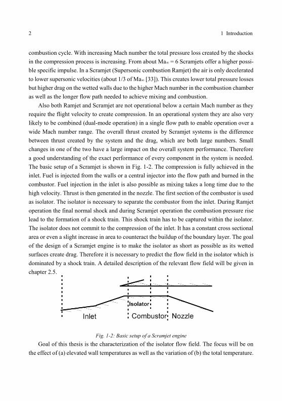
The basic setup of a Scramjet is shown in Fig. 1-2. The compression is fully achieved in the
inlet. Fuel is injected from the walls or a central injector into the flow path and burned in the
combustor. Fuel injection in the inlet is also possible as mixing takes a long time due to the
high velocity. Thrust is then generated in the nozzle. The first section of the combustor is used
as isolator. The isolator is necessary to separate the combustor from the inlet. During Ramjet
operation the final normal shock and during Scramjet operation the combustion pressure rise
lead to the formation of a shock train. This shock train has to be captured within the isolator.
The isolator does not commit to the compression of the inlet. It has a constant cross sectional
area or even a slight increase in area to counteract the buildup of the boundary layer. The goal
of the design of a Scramjet engine is to make the isolator as short as possible as its wetted
surfaces create drag. Therefore it is necessary to predict the flow field in the isolator which is
dominated by a shock train. A detailed description of the relevant flow field will be given in
chapter 2.5.
Fig. 1-2: Basic setup of a Scramjet engine
Goal of this thesis is the characterization of the isolator flow field. The focus will be on
the effect of (a) elevated wall temperatures as well as the variation of (b) the total temperature.
1.2 Research training group 1095 3
Experiments and numerical simulations are carried out using an isolator in a typical Scramjet
configuration. For a better understanding of underlying mechanisms of the shock train flow a
simplified configuration with symmetric inflow will also be investigated. As both configura-
tions feature a rectangular cross section a third model with variable width will also be inves-
tigated to study 3D effects. The results will be compared to existing correlations for shock
train flows and these correlations will be expanded to cover the effects investigated.
For the Scramjet configuration the flow entering the isolator is not uniform. The final
compression shock that originates from the leading edge of the lip induces a separation bubble
on the ramp. The wall and total temperature effect on this separation bubble will also be in-
vestigated. It will also be discussed whether a boundary bleed is feasible here in order to
reduce losses.
1.2 Research training group 1095
1.2.1 Overview
The presented research is part of Germany’s research training group (GRK) 1095 “Aero-
Thermodynamic Design of a Scramjet Propulsion System for Future Space Transportation
Systems” which studies a Scramjet propulsion system with experimental, numerical and ana-
lytical means as well as from the conceptional point of view. It is a collaborative project of
institutes at the University of Stuttgart, the Technical University of Munich, RWTH Aachen
University and the DLR in Cologne. In an additional subproject combustion tests with a
scramjet model are conducted at ITAM, Novosibirsk in Russia. The Research Training Group
started in 2005 and is divided into 3 periods. The presented research was done in the second
phase. The goal of the research training group is the design of a scramjet engine on paper. An
optimized Scramjet configuration for flight tests is developed as a goal of the research training
group but a flight test is not part of the project.
1.2.2 Context for presented research
The model and therewith the inlet and isolator flow path that is the core of the investiga-
tions of this thesis was designed during the first phase [31], [67]. Two almost identical inlet
models were built to be tested at the DLR in Cologne as well as at the Shock Wave Laboratory
(SWL) in Aachen. The tests at the DLR focused on the operational behavior of the inlet at
different yaw angles [38] and additional sidewall compression [37]. A shock train was also
generated with varying back pressure [29].
In the second phase of the research training group an additional three dimensional inlet
was designed for a potential flight test configuration [28]. The research presented here uses
4 1 Introduction
the model design from the first phase to investigate more fundamental flow phenomena in the
isolator. Results from the experiments are also used as validation data for numerical subpro-
jects [69]. An overview of the structure as well as the full research profile of the research
training group can be found in [28] and [103].
5
f
S
2 Fundamentals
2.1 Navier Stokes equations
To reach an analytical description for any kind of flow the three basic conservation laws
for mass, momentum and energy are used. The mass of a defined number of material elements
is constant (eq. 2.1) while the volume can be a function of time.
)()(
0.
tVtV
dVdt
d
dt
dmconstdVm (2.1)
This leads to the mass conservation equation:
.0
z
w
y
v
x
u
t
(2.2)
For the momentum conservation the product of mass and acceleration is the sum for all
forces per volume element. They consist of mass forces per volume element (e.g. force of
gravity on the material elements; often neglected) and the surface forces per volume element
(stresses and pressure) (eq. 2.3).
SfDt
uD
(2.3)
The complete derivation of the surface forces can be found in [80]. This leads to the mo-
mentum conservation of the Navier Stokes equations in x (eq. 2.4), y (eq. 2.5), and z (eq. 2.6)
direction. It is assumed that the volume viscosity is of smaller magnitude than the dynamic
viscosity (Stokes Hypothesis) and can therefore be neglected.
6 2 Fundamentals
z
u
x
w
zx
v
y
u
y
z
w
y
v
x
u
x
u
xx
pf
dt
dux
3
22
(2.4)
x
v
y
u
xy
w
z
v
z
z
w
y
v
x
u
y
v
yy
pf
dt
dvy
3
22
(2.5)
y
w
z
v
yz
u
x
w
x
z
w
y
v
x
u
z
w
zz
pf
dt
dwz
3
22
(2.6)
For the conservation of energy the change of internal energy of a material element is given
by the heat transfer and the work performed on the element (eq. 2.7).
WQdt
de (2.7)
The derivation of the complete energy conservation (eq. 2.8) of the Navier Stokes equa-
tions can again be found in [80].
2.1 Navier Stokes equations 7
222
2222
3
22
x
w
z
u
z
v
y
w
x
u
x
v
z
w
y
v
x
u
z
w
y
v
x
u
z
Tk
zy
Tk
yx
Tk
xz
w
y
v
x
up
dt
de
(2.8)
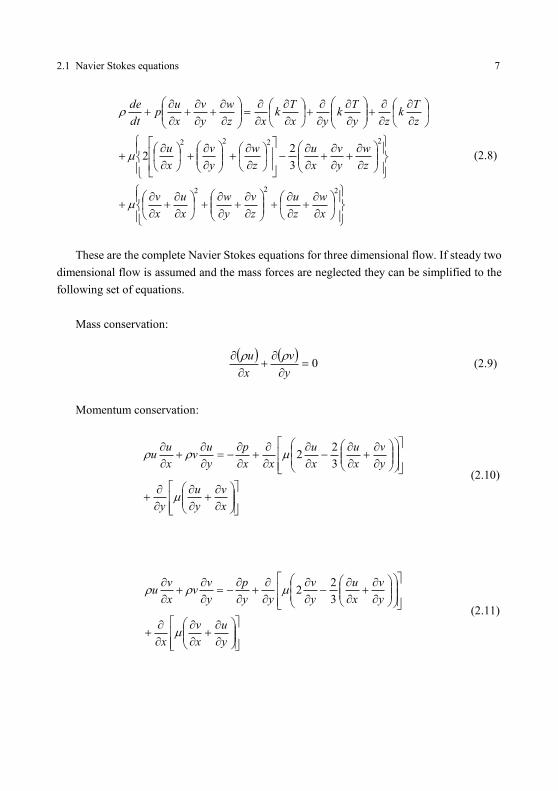
These are the complete Navier Stokes equations for three dimensional flow. If steady two
dimensional flow is assumed and the mass forces are neglected they can be simplified to the
following set of equations.
Mass conservation:
0
y
v
x
u (2.9)
Momentum conservation:
x
v
y
u
y
y
v
x
u
x
u
xx
p
y
uv
x
uu
3
22
(2.10)
y
u
x
v
x
y
v
x
u
y
v
yy
p
y
vv
x
vu
3
22
(2.11)
8 2 Fundamentals
Energy conservation:
2222
3
22
x
u
x
v
y
v
x
u
y
v
x
u
y
Tk
yx
Tk
xy
v
x
up
dt
de
(2.12)
2.2 Boundary layer flow
2.2.1 Laminar boundary layers
The Navier Stokes equations for steady flow can be further simplified for flow fields over
wetted surfaces to obtain the laminar boundary layer equations by the estimation of the mag-
nitude of the single terms. Therefore the flow field is divided into two parts. In the outer,
inviscid part heat conduction and friction can be neglected. For the flow over a flat plate the
conditions are constant (e) along the boundary layer edge. In a thin layer close to the wall the
flow is dominated by heat conduction and friction. This is the boundary layer [77] and here
flow properties are changing from wall to edge conditions. The following assumptions are
taken.
The boundary layer is thin compared to the characteristic length (L) of the flow
case (δ/L<<1). On the flat plate this is the running length of the boundary layer
on the plate.
The Reynolds number is large.
The boundary layer thickness and the velocity in y-direction are inversely pro-
portional to the square root of the Reynolds number.
The Reynolds number is defined in equation 2.13.
uLx Re (2.13)
The first assumption leads to the boundary layer theory being not valid close to leading
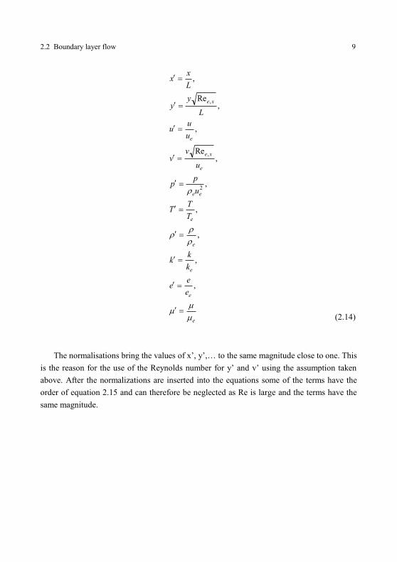
edges. Then all quantities in the Navier Stokes equations are normalized as stated in (eq. 2.14).
This leads to the boundary layer equations. The detailed derivation can be found in [80].
2.2 Boundary layer flow 9
e
e
e
e
e
ee
e
xe
e
xe
e
ee
k
kk
T
TT
u
pp
u
vv
u
uu
L
yy
L
xx
,
,
,
,
,
,Re
,
,Re
,
2
,
,
(2.14)
The normalisations bring the values of x’, y’,… to the same magnitude close to one. This
is the reason for the use of the Reynolds number for y’ and v’ using the assumption taken
above. After the normalizations are inserted into the equations some of the terms have the
order of equation 2.15 and can therefore be neglected as Re is large and the terms have the
same magnitude.
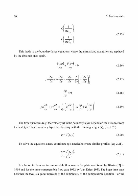
10 2 Fundamentals
2,
,
Re
1
,Re
1
xe
xe
O
O
(2.15)
This leads to the boundary layer equations where the normalized quantities are replaced
by the absolute ones again.
0
y
v
x
u (2.16)
y
u
yx
p
y
vv
x
uu (2.17)
0
y
p (2.18)
2
y
u
dx
dpu
y
Tk
yy
hv
x
hu (2.19)
The flow quantities (e.g. the velocity u) in the boundary layer depend on the distance from
the wall (y). These boundary layer profiles vary with the running length (x), (eq. 2.20).
yxfu , (2.20)
To solve the equations a new coordinate η is needed to create similar profiles (eq. 2.21).
fu
yxf
,, (2.21)
A solution for laminar incompressible flow over a flat plate was found by Blasius [7] in
1908 and for the same compressible flow case 1952 by Van Driest [95]. The huge time span
between the two is a good indicator of the complexity of the compressible solution. For the
2.2 Boundary layer flow 11
Van Driest solution the fluid has to be ideal and calorically perfect (eq. 2.22 and eq. 2.23).
Also the Prandl number Pr is assumed to be constant (eq. 2.24).
Tch p (2.22)
RTp (2.23)
.Pr constk
c
(2.24)
Also the viscosity relation µ/µ∞ needs to be described as a function of temperature. The
viscosity can be modeled either with a simple power law (eq. 2.25) or with the Sutherland law
(eq. 2.26). The appropriate exponent ω changes with temperature and the factor cµ with ω. For
low temperatures (T ≤ 200 K) ω = 1 is adequate. For higher temperatures (T ≥ 400 K)
ω = 0.65 is used [36]. With the power law the viscosity relation can be obtained as function
of T/T∞ only, if ω is identical for both temperatures (eq. 2.27). This is not possible with the
Sutherland law (eq. 2.28). Still Van Driest used the Sutherland law to obtain the viscosity
relation µ/µ∞ as a function of T/T∞ and T∞ as he found the power law with a constant exponent
ω to be less accurate for the viscosity than the Sutherland law. Therefore the boundary profiles
calculated by him are all set to a specific free stream temperature.
With the application of the power law the calculation procedure is possible without using
a specific temperature T∞ but will create less accurate data. Significantly different wall or free
stream temperatures at a constant relation will result in identical profiles. This is not correct,
as the exponent ω is a function of temperature.
12 2 Fundamentals
Tc (2.25)
ST
TC
5.1
(2.26)
ee T
T (2.27)
ST
ST
T
Te
ee
5.1
(2.28)
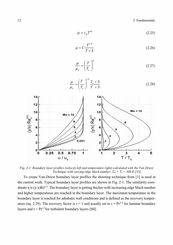
Fig. 2-1: Boundary layer profiles (velocity left and temperature right) calculated with the Van Driest
Technique with varying edge Mach number; TW = Te = 300 K [35]
To create Van-Driest boundary layer profiles the shooting technique from [1] is used in
the current work. Typical boundary layer profiles are shown in Fig. 2-1. The similarity coor-
dinate η is (y/x)Re0.5. The boundary layer is getting thicker with increasing edge Mach number
and higher temperatures are reached in the boundary layer. The maximum temperature in the
boundary layer is reached for adiabatic wall conditions and is defined as the recovery temper-
ature (eq. 2.29). The recovery factor is r < 1 and usually set to r = Pr1/2 for laminar boundary
layers and r = Pr1/3for turbulent boundary layers [80].
2.2 Boundary layer flow 13
2
2
11 eer rMaTT
(2.29)
In Fig. 2-1 it is shown that it is not possible to separate the boundary layer sharply from
the outer flow field. Therefore no natural definition of the boundary layer thickness is availa-
ble. Usually the definition in equation 2.30 is used with ε = 0.01 [80].
ee uyuu )( (2.30)
For the incompressible boundary layer this results in [7]:
.
Re9.4
,xe
x (2.31)
For correlations often two other definitions of the boundary layer thickness are used. The
boundary layer displacement thickness δ1 (eq. 2.32) describes the offset of the outer flow field
away from the wetted wall caused by the boundary layer in case of an equivalent inviscid
flow. The boundary layer momentum thickness δ2 (eq. 2.33) describes the momentum loss
caused by the boundary layer in the term of the thickness of flow at edge conditions repre-
senting this loss.
y
y ee
dyu
u
0
1 1 (2.32)
y
y eee
dyu
u
u
u
0
2 1 (2.33)
14 2 Fundamentals
The wall shear stress (eq. 2.34) and the skin-friction coefficient (eq. 2.35) can also be
calculated from the boundary layer profile.
W
WWy
u
(2.34)
e
Wf
qc
(2.35)
The wall heat transfer can be deduced for flat plate flow at constant wall temperature from
the skin friction with the Reynolds analogy [80] using the recovery temperature defined in
equation 2.29:
).(Pr2
3/2wrpee
ee
WW TTcu
uq
(2.36)
Then the Stanton number CH can be calculated. For practical reasons here the Stanton
number is calculated with the total temperature instead of the reference temperature (eq. 2.29)
as the reference temperature depends on local edge conditions and therewith on the local
model geometry and the state of the boundary layer.
Wpee
WH
TTcu
qC
0
(2.37)
As an alternative to the elaborate calculation of the boundary layer in the Van Driest
method the reference temperature method [23] can be used. For incompressible flow the tem-
perature in the boundary layer is identical to the edge temperature. The quantities ρ and µ
which depend on the temperature are identical to the edge conditions. Based on empirical
observations the wall shear stress and wall heat transfer can be obtained for compressible flow
based on the calculations for incompressible flow. Therefore the density ρ and the viscosity µ
are calculated at a reference temperature (eq. 2.38). It combines the values of the fluid at the
wall (W), at the boundary layer edge (e) and the recovery values (r, eq. 2.29).
2.2 Boundary layer flow 15
rWe TTTT 22.05.028.0* (2.38)
If the pressure is constant through the boundary layer normal to the wetted surface equa-
tion 2.23 can be simplified to:
..**eeTconstT (2.39)
This is used to calculate density as a function of temperature. The viscosity relation µ/µe
is calculated as a function of temperature relation T/Te with equation 2.27 using the power
law with a constant exponent ω. The Sutherland law is not used here due to its more complex
structure. As an example the Reynolds number is transformed to reference conditions:
.ReRe
1
*,*
*
*
**
T
Txuxu exe
e
ee
eeex (2.40)
The same principle is used to obtain the skin friction (eq. 2.41) and wall heat transfer
(eq. 2.42) for compressible flow [36].
)1(5.0*
,
2
Re332.0
exe
eeW
T
Tu (2.41)
xT
TTTkq
e
wreW
Re)(Pr332.0
)1(5.0*
3/1
(2.42)
Here k is the thermal conductivity. It can also be calculated with a power law [36]:
75.0510957.34 Tk (2.43)
16 2 Fundamentals
According to Simeonides [84], Hirschel [36] and others based on the reference tempera-
ture the boundary layer displacement and momentum thickness can be expressed as follows:
15.0
*2
,
12
1333.0122.1122.0
Re72.1
e
e
e
W
xeT
TMa
T
Tx (2.44)
15.0*
,
2Re
66.0
exe
T
Tx (2.45)
2.2.2 Turbulent boundary layers
In chapter 2.2.1 the boundary layer equations were derived assuming steady flow. From a
certain Reynolds number upward (and therewith a certain boundary layer running length) the
boundary layer flow can become instable resulting in a turbulent boundary layer [78]. For
defined flow conditions the boundary layer transitions to turbulent after a certain running
length. Still the Reynolds number is not the only influencing parameter. In [1] 19 influencing
parameters are listed including the surface structure.
Based on empirical observation a power formula can be used to describe the mean flow
field of an incompressible turbulent boundary layer (eq. 2.46) [80].
7
1
y
u
u
e
(2.46)
Then the reference temperature can be used to obtain the skin friction (eq. 2.47), the wall
heat transfer (eq. 2.48), the boundary layer displacement thickness (eq. 2.49) and the momen-
tum thickness (eq. 2.50) [36].
)4(2.0*
2.0,Re
0592.0
exe
e
fT
Tuc (2.47)
2.2 Boundary layer flow 17
8.02.0)4(2.0
*3/1 Re
1)(Pr0296.0
xT
TTTkq
e
wreW
(2.48)
42.0*
2
2.0,
12
1648.0871.0129.0
Re0504.0
e
e
e
W
xeT
TMa
T
Tx (2.49)
42.0*
2.0,
2Re
036.0
exe
T
Tx (2.50)
Using the reference temperature the boundary layer quantities, except the wall heat trans-
fer, become a function of the relation between wall and edge temperature only if the power
law exponent ω is constant and therefore identical for edge, wall and reference conditions.
The data becomes less accurate with increasing differences for these values. Still it is the only
way to quickly obtain all the desired boundary layer parameters for turbulent flow. The wall
heat transfer and the wall skin friction but not the boundary layer displacement and momen-
tum thickness can be calculated from the boundary layer equations as shown in [94].
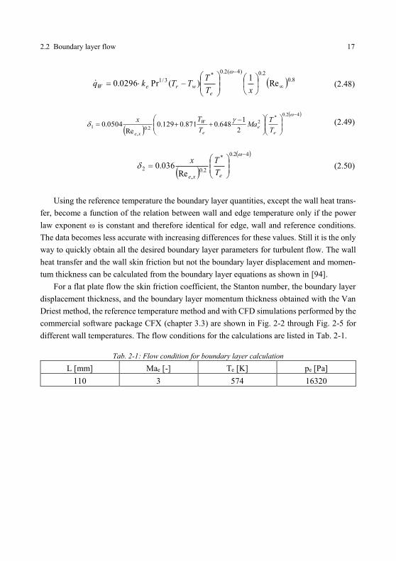
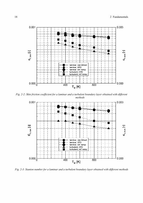
For a flat plate flow the skin friction coefficient, the Stanton number, the boundary layer
displacement thickness, and the boundary layer momentum thickness obtained with the Van
Driest method, the reference temperature method and with CFD simulations performed by the
commercial software package CFX (chapter 3.3) are shown in Fig. 2-2 through Fig. 2-5 for
different wall temperatures. The flow conditions for the calculations are listed in Tab. 2-1.
Tab. 2-1: Flow condition for boundary layer calculation
L [mm] Mae [-] Te [K] pe [Pa]
110 3 574 16320
18 2 Fundamentals
Fig. 2-2: Skin friction coefficient for a laminar and a turbulent boundary layer obtained with different methods
Fig. 2-3: Stanton number for a laminar and a turbulent boundary layer obtained with different methods
2.2 Boundary layer flow 19
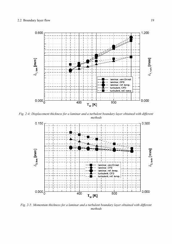
Fig. 2-4: Displacement thickness for a laminar and a turbulent boundary layer obtained with different methods
Fig. 2-5: Momentum thickness for a laminar and a turbulent boundary layer obtained with different methods
20 2 Fundamentals
For the laminar boundary layer all three calculation methods result in almost identical
values for the boundary layer parameters. For the turbulent boundary layer the results are of
the same magnitude and the wall temperature effect is captured qualitatively identical with
the two methods available here. Still an offset of up to about 10 % exists between results of
the CFD simulations and the reference temperature method. Later to predict the pressure dis-
tribution inside a shock train the Stanton number and the boundary layer momentum thickness
will be used with an exponent of 0.25. The offset of 10 % between the values is not problem-
atic here and the easily available values from the reference temperature method will be used
for correlation purposes.
2.3 Shock boundary layer interaction
If a supersonic boundary layer is hit by a compression shock this can result in local flow
separation. The dynamic pressure in the boundary layer is reduced by friction. When the
boundary layer is subject to the pressure rise by a compression shock it might not be able
follow this pressure rise. This results in the separation of the boundary layer. Two typical
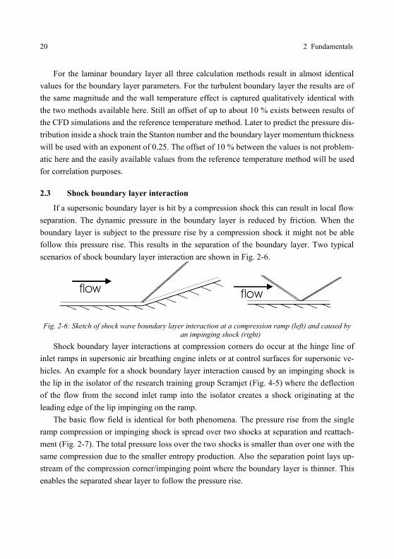
scenarios of shock boundary layer interaction are shown in Fig. 2-6.
Fig. 2-6: Sketch of shock wave boundary layer interaction at a compression ramp (left) and caused by an impinging shock (right)
Shock boundary layer interactions at compression corners do occur at the hinge line of
inlet ramps in supersonic air breathing engine inlets or at control surfaces for supersonic ve-
hicles. An example for a shock boundary layer interaction caused by an impinging shock is
the lip in the isolator of the research training group Scramjet (Fig. 4-5) where the deflection
of the flow from the second inlet ramp into the isolator creates a shock originating at the
leading edge of the lip impinging on the ramp.
The basic flow field is identical for both phenomena. The pressure rise from the single
ramp compression or impinging shock is spread over two shocks at separation and reattach-
ment (Fig. 2-7). The total pressure loss over the two shocks is smaller than over one with the
same compression due to the smaller entropy production. Also the separation point lays up-
stream of the compression corner/impinging point where the boundary layer is thinner. This
enables the separated shear layer to follow the pressure rise.
2.3 Shock boundary layer interaction 21
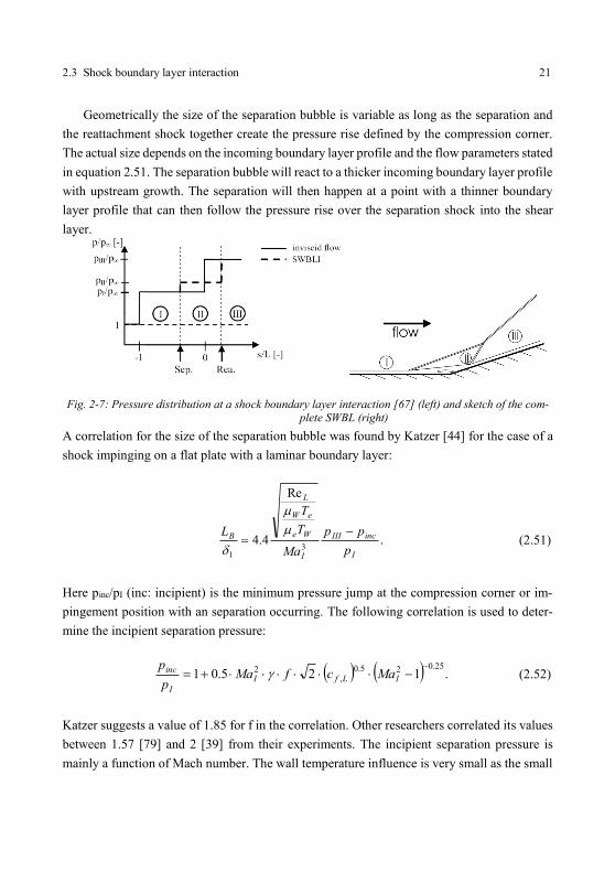
Geometrically the size of the separation bubble is variable as long as the separation and
the reattachment shock together create the pressure rise defined by the compression corner.
The actual size depends on the incoming boundary layer profile and the flow parameters stated
in equation 2.51. The separation bubble will react to a thicker incoming boundary layer profile
with upstream growth. The separation will then happen at a point with a thinner boundary
layer profile that can then follow the pressure rise over the separation shock into the shear
layer.
Fig. 2-7: Pressure distribution at a shock boundary layer interaction [67] (left) and sketch of the com-plete SWBL (right)
A correlation for the size of the separation bubble was found by Katzer [44] for the case of a
shock impinging on a flat plate with a laminar boundary layer:
.
Re
4.43
1 I
incIII
I
We
eW
L
B
p
pp
Ma
T
T
L
(2.51)
Here pinc/pI (inc: incipient) is the minimum pressure jump at the compression corner or im-
pingement position with an separation occurring. The following correlation is used to deter-
mine the incipient separation pressure:
.125.0125.025.0
,2
ILfI
I
inc MacfMap
p (2.52)
Katzer suggests a value of 1.85 for f in the correlation. Other researchers correlated its values
between 1.57 [79] and 2 [39] from their experiments. The incipient separation pressure is
mainly a function of Mach number. The wall temperature influence is very small as the small
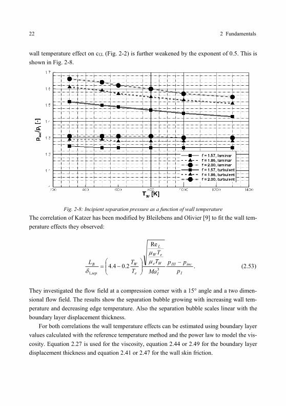
22 2 Fundamentals
wall temperature effect on cf,L (Fig. 2-2) is further weakened by the exponent of 0.5. This is
shown in Fig. 2-8.
Fig. 2-8: Incipient separation pressure as a function of wall temperature
The correlation of Katzer has been modified by Bleilebens and Olivier [9] to fit the wall tem-
perature effects they observed:
.
Re
2.04.43
,1 I
incIII
I
We
eW
L
e
W
sep
B
p
pp
Ma
T
T
T
TL
(2.53)
They investigated the flow field at a compression corner with a 15° angle and a two dimen-
sional flow field. The results show the separation bubble growing with increasing wall tem-
perature and decreasing edge temperature. Also the separation bubble scales linear with the
boundary layer displacement thickness.
For both correlations the wall temperature effects can be estimated using boundary layer
values calculated with the reference temperature method and the power law to model the vis-
cosity. Equation 2.27 is used for the viscosity, equation 2.44 or 2.49 for the boundary layer
displacement thickness and equation 2.41 or 2.47 for the wall skin friction.
2.3 Shock boundary layer interaction 23
The shock wave boundary layer interaction at the hinge line of the two compression ramps
of the inlet model used in this thesis was investigated prior to this work by Neuenhahn and
Olivier [66]. They also showed a growing separation bubble with increasing wall and decreas-
ing edge temperature. In addition they showed that the separation length is not only a factor
of the relation between wall and edge temperature (TW/Te) but also the edge (or wall) temper-
ature itself. The separation bubble reacts extremely sensitive to the incoming boundary layer
profile therefore the use of the power law with a constant exponent ω to calculate the viscosity
µ is not applicable here. Neuenhahn [67] also developed a correlation for the separation bub-
ble length based on the momentum equation for the free shear layer over the separation bub-
ble. In that correlation (eq. 2.54) also the empirically correlated incipient separation pressure
is used and the difference of the shear stress on the upper and lower boundary of the free shear
layer is estimated with the half value of the wall skin friction at the separation point for the
undisturbed boundary layer based on empirical observation. The values for the skin friction
coefficient cf and the sonic height factor Ch can be obtained from boundary layer calculation
e.g. using the Van Driest method described above. For the incipient separation pressure pinc
data has to be gained from empirical correlations or be predicted otherwise (e.g. by numerical
simulations).
I
incIII
If
hB
p
pp
Ma
x
c
CL
2Re
4
(2.54)
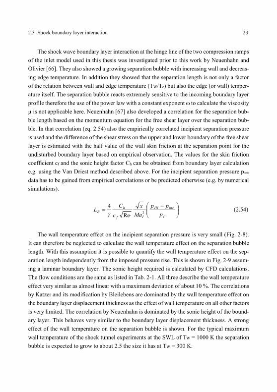
The wall temperature effect on the incipient separation pressure is very small (Fig. 2-8).
It can therefore be neglected to calculate the wall temperature effect on the separation bubble
length. With this assumption it is possible to quantify the wall temperature effect on the sep-
aration length independently from the imposed pressure rise. This is shown in Fig. 2-9 assum-
ing a laminar boundary layer. The sonic height required is calculated by CFD calculations.
The flow conditions are the same as listed in Tab. 2-1. All three describe the wall temperature
effect very similar as almost linear with a maximum deviation of about 10 %. The correlations
by Katzer and its modification by Bleilebens are dominated by the wall temperature effect on
the boundary layer displacement thickness as the effect of wall temperature on all other factors
is very limited. The correlation by Neuenhahn is dominated by the sonic height of the bound-
ary layer. This behaves very similar to the boundary layer displacement thickness. A strong
effect of the wall temperature on the separation bubble is shown. For the typical maximum
wall temperature of the shock tunnel experiments at the SWL of TW = 1000 K the separation
bubble is expected to grow to about 2.5 the size it has at TW = 300 K.
24 2 Fundamentals
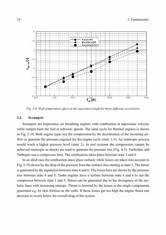
Fig. 2-9: Wall temperature effect on the separation length for three different correlations
2.4 Scramjets
Scramjets are hypersonic air breathing engines with combustion at supersonic velocity
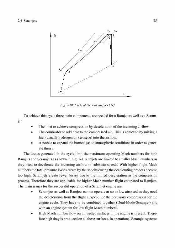
while ramjets burn the fuel at subsonic speeds. The ideal cycle for thermal engines is shown
in Fig. 2-10. Both engine types use the compression by the deceleration of the incoming air-
flow to generate the pressure required for the engine cycle (state 1-3). An isentropic process
would reach a higher pressure level (state 2). In real systems the compression cannot be
achieved isentropic as shocks are used to generate the pressure rise (Fig. 4-5). Turbofans and
Turbojets use a compressor here. The combustion takes place between state 3 and 4.
In an ideal case the combustion takes place isobaric while losses are taken into account in
Fig. 2-10 shown by the drop of the pressure from the isobaric line starting at state 3. The thrust
is generated by the expansion between state 4 and 6. The losses here are shown by the pressure
loss between state 4 and 5. Turbo engines have a turbine between state 4 and 6 to run the
compressor between state 1 and 3. Thrust can be generated due to the divergence of the iso-
baric lines with increasing entropy. Thrust is lowered by the losses in the single components
generated e.g. by skin friction on the walls. If these losses get too high the engine thrust can
decrease to levels below the overall drag of the system.
2.4 Scramjets 25
Fig. 2-10: Cycle of thermal engines [34]
To achieve this cycle three main components are needed for a Ramjet as well as a Scram-
jet.
The inlet to achieve compression by deceleration of the incoming airflow
The combustor to add heat to the compressed air. This is achieved by mixing a
fuel (usually hydrogen or kerosene) into the airflow.
A nozzle to expand the burned gas to atmospheric conditions in order to gener-
ate thrust.
The losses generated in the cycle limit the maximum operating Mach numbers for both
Ramjets and Scramjets as shown in Fig. 1-1. Ramjets are limited to smaller Mach numbers as
they need to decelerate the incoming airflow to subsonic speeds. With higher flight Mach
numbers the total pressure losses create by the shocks during the decelerating process become
too high. Scramjets create fewer losses due to the limited deceleration in the compression
process. Therefore they are applicable for higher Mach number flight compared to Ramjets.
The main issues for the successful operation of a Scramjet engine are:
Scramjets as well as Ramjets cannot operate at no or low airspeed as they need
the deceleration from the flight airspeed for the necessary compression for the
engine cycle. They have to be combined together (Dual-Mode-Scramjet) and
with an engine system for low flight Mach numbers
High Mach number flow on all wetted surfaces in the engine is present. There-
fore high drag is produced on all these surfaces. In operational Scramjet systems
26 2 Fundamentals
overall drag and net thrust are close values of the same magnitude. The overall
system performance reacts sensitive to small changes in the single system com-
ponents.
For an effective Scramjet engine the area of the wetted surfaces and therewith the length
of the engine flow path should be as short as possible. To achieve an effective compression in
the inlet low compression angles and multiple shocks are desirable. An efficient compression
in the inlet also has the advantage that the air is reaching lower temperatures at the end of the
process. This leaves more margins for the addition of heat in the combustion process. Still
both measures create larger areas of wetted surfaces. For the combustion process a rather long
internal flow path is needed to mix the injected fuel before it can be burned. Here again this
results in more drag due to skin friction. The simple basic design of a Scramjet has to be
optimized to build a working engine.
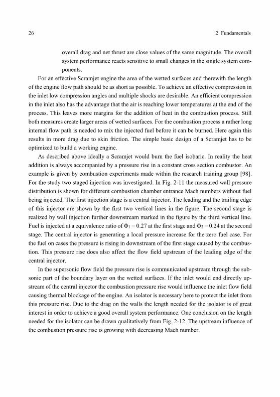
As described above ideally a Scramjet would burn the fuel isobaric. In reality the heat
addition is always accompanied by a pressure rise in a constant cross section combustor. An
example is given by combustion experiments made within the research training group [98].
For the study two staged injection was investigated. In Fig. 2-11 the measured wall pressure
distribution is shown for different combustion chamber entrance Mach numbers without fuel
being injected. The first injection stage is a central injector. The leading and the trailing edge
of this injector are shown by the first two vertical lines in the figure. The second stage is
realized by wall injection further downstream marked in the figure by the third vertical line.
Fuel is injected at a equivalence ratio of Φ1 = 0.27 at the first stage and Φ2 = 0.24 at the second
stage. The central injector is generating a local pressure increase for the zero fuel case. For
the fuel on cases the pressure is rising in downstream of the first stage caused by the combus-
tion. This pressure rise does also affect the flow field upstream of the leading edge of the
central injector.
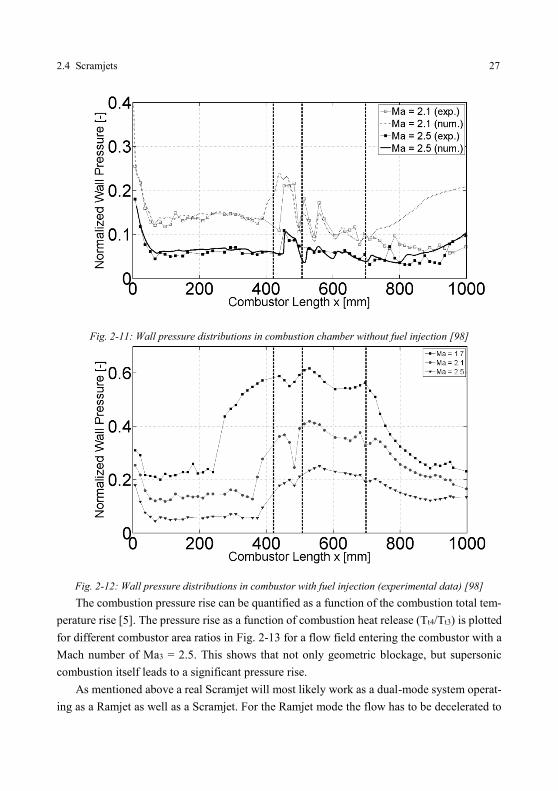
In the supersonic flow field the pressure rise is communicated upstream through the sub-
sonic part of the boundary layer on the wetted surfaces. If the inlet would end directly up-
stream of the central injector the combustion pressure rise would influence the inlet flow field
causing thermal blockage of the engine. An isolator is necessary here to protect the inlet from
this pressure rise. Due to the drag on the walls the length needed for the isolator is of great
interest in order to achieve a good overall system performance. One conclusion on the length
needed for the isolator can be drawn qualitatively from Fig. 2-12. The upstream influence of
the combustion pressure rise is growing with decreasing Mach number.
2.4 Scramjets 27
Fig. 2-11: Wall pressure distributions in combustion chamber without fuel injection [98]
Fig. 2-12: Wall pressure distributions in combustor with fuel injection (experimental data) [98]
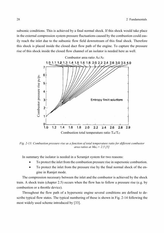
The combustion pressure rise can be quantified as a function of the combustion total tem-
perature rise [5]. The pressure rise as a function of combustion heat release (Tt4/Tt3) is plotted
for different combustor area ratios in Fig. 2-13 for a flow field entering the combustor with a
Mach number of Ma3 = 2.5. This shows that not only geometric blockage, but supersonic
combustion itself leads to a significant pressure rise.
As mentioned above a real Scramjet will most likely work as a dual-mode system operat-
ing as a Ramjet as well as a Scramjet. For the Ramjet mode the flow has to be decelerated to
28 2 Fundamentals
subsonic conditions. This is achieved by a final normal shock. If this shock would take place
in the external compression system pressure fluctuations caused by the combustion could eas-
ily reach the inlet due to the subsonic flow field downstream of this final shock. Therefore
this shock is placed inside the closed duct flow path of the engine. To capture the pressure
rise of this shock inside the closed flow channel of an isolator is needed here as well.
Fig. 2-13: Combustion pressure rise as a function of total temperature ratio for different combustor area ratios at Ma3 = 2.5 [5]
In summary the isolator is needed in a Scramjet system for two reasons:
To protect the inlet from the combustion pressure rise in supersonic combustion.
To protect the inlet from the pressure rise by the final normal shock of the en-
gine in Ramjet mode.
The compression necessary between the inlet and the combustor is achieved by the shock
train. A shock train (chapter 2.5) occurs when the flow has to follow a pressure rise (e.g. by
combustion or a throttle device).
Throughout the flow path of a hypersonic engine several conditions are defined to de-
scribe typical flow states. The typical numbering of these is shown in Fig. 2-14 following the
most widely used scheme introduced by [33].
Combustor area ratio A4/A3
Combustion total temperature ratio Tt4/Tt3
Co
mb
ust
or
pre
ssu
re r
ise
p4/p
3
2.4 Scramjets 29
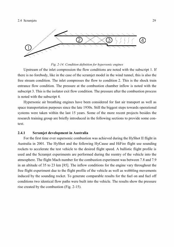
Fig. 2-14: Condition definition for hypersonic engines
Upstream of the inlet compression the flow conditions are noted with the subscript 1. If
there is no forebody, like in the case of the scramjet model in the wind tunnel, this is also the
free stream condition. The inlet compresses the flow to condition 2. This is the shock train
entrance flow condition. The pressure at the combustion chamber inflow is noted with the
subscript 3. This is the isolator exit flow condition. The pressure after the combustion process
is noted with the subscript 4.
Hypersonic air breathing engines have been considered for fast air transport as well as
space transportation purposes since the late 1930s. Still the biggest steps towards operational
systems were taken within the last 15 years. Some of the more recent projects besides the
research training group are briefly introduced in the following sections to provide some con-
text.
2.4.1 Scramjet development in Australia
For the first time ever supersonic combustion was achieved during the HyShot II flight in
Australia in 2001. The HyShot and the following HyCause and HiFire flight use sounding
rockets to accelerate the test vehicle to the desired flight speed. A ballistic flight profile is
used and the Scramjet experiments are performed during the reentry of the vehicle into the
atmosphere. The flight Mach number for the combustion experiment was between 7.8 and 7.9
in an altitude of 35 to 23 km [85]. The inflow conditions for the engine vary throughout the
free flight experiment due to the flight profile of the vehicle as well as wobbling movements
induced by the sounding rocket. To generate comparable results for the fuel on and fuel off
conditions two identical flow paths were built into the vehicle. The results show the pressure
rise created by the combustion (Fig. 2-15).
30 2 Fundamentals
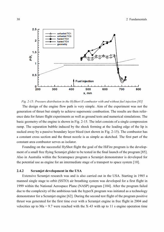
Fig. 2-15: Pressure distribution in the HyShort II combustor with and without fuel injection [85]
The design of the engine flow path is very simple. Aim of the experiment was not the
generation of thrust but simply to achieve supersonic combustion. The results are then refer-
ence data for future flight experiments as well as ground tests and numerical simulations. The
basic geometry of the engine is shown in Fig. 2-15. The inlet consists of a single compression
ramp. The separation bubble induced by the shock forming at the leading edge of the lip is
sucked away by a passive boundary layer bleed (not shown in Fig. 2-15). The combustor has
a constant cross section and the thrust nozzle is as simple as sketched. The first part of the
constant area combustor serves as isolator.
Founding on the successful HyShot flight the goal of the HiFire program is the develop-
ment of a small free flying Scramjet glider to be tested in the final launch of the program [85].
Also in Australia within the Scramspace program a Scramjet demonstrator is developed for
the potential use as engine for an intermediate stage of a transport to space system [10].
2.4.2 Scramjet development in the USA
Extensive Scramjet research was and is also carried out in the USA. Starting in 1985 a
manned single stage to orbit (SSTO) air breathing system was developed for a first flight in
1999 within the National Aerospace Plane (NASP) program [104]. After the program failed
due to the complexity of the ambitious task the hyperX program was initiated as a technology
demonstrator for a Scramjet engine [62]. During the second test flight of the program positive
thrust was generated for the first time ever with a Scramjet engine in free flight in 2004 and
velocities up to Ma = 9.7 were reached with the X-43 with up to 11 s engine operation time
2.5 Shock trains 31
[59]. This was then followed by the X-51 with a first flight in 2010. It was flying at a lower
Mach number of Ma = 5 with Kerosene as fuel operating for 200 s, to develop an engine for
continuous operation [93].
2.5 Shock trains
Shock trains were first observed in 1949 in the diffusers of supersonic wind tunnels [68].
The expected discontinuous pressure jump of a single shock occurred over a longer distance.
Shock trains occur in closed duct flows if a sufficiently strong pressure rise is forced on the
flow. The overall pressure rise is limited by the pressure jump over a single normal shock.
The pressure rise is communicated upstream through the subsonic part of the boundary layers
on the wetted surfaces. A shock train can also develop if the pressure rise over a single shock
in a closed duct is too high for the boundary layer to follow, leading to the separation and
therewith upstream movement of the first shock. If boundary layers are present a single normal
shock in a closed duct is usually only possible at very low supersonic Mach numbers.
Two different types of shock trains are known:
The normal shock train with a strong normal shock with lambda feet at the be-
ginning followed by weaker normal shocks. Downstream of the first shock the
flow is accelerated back to supersonic speed and a new weaker shock occurs. It
takes numerous shocks till the flow at the end of the shock train is subsonic. The
flow field is sketched in Fig. 2-16.
The oblique shock train initialized by oblique shocks. Here the pressure rise is
lower at the beginning of the shock train. The flow can be either subsonic or
supersonic after passing the shock train. Therefore an oblique shock train can
also contain weak normal shocks towards the end.
Fig. 2-16: Drawing of a normal shock train flow field
32 2 Fundamentals
Fig. 2-17: Drawing of an oblique shock train flow field with supersonic exit flow
The beginning of the shock train is the first pressure jump caused by the first shock. If the
shock train is caused by a pressure rise (e.g. a combustion pressure rise) the location of this
pressure rise marks the end of the shock train. If the shock train is caused by a single normal
shock interacting with the boundary layer the exit plane is defined by a uniform pressure and
total pressure profile being reached. The normal shock train can be divided into two parts. In
the first part which is the upstream region the supersonic flow is gradually decelerated and in
the second downstream region the high speed flow in the central core is mixed with the low
speed flow near the walls [90]. The main influencing factor on the type of shock train occur-
ring is the isolator entrance Mach number Ma2. Usually the transition between normal and
oblique shock train happens between Ma2 = 2 and Ma2 = 3.
A typical example for a normal shock train is given in Fig. 2-18 from [89]. Shown are the
pressure distributions at the wall and at the centerline of the flow channel. The flow field is
additionally illustrated with pressure contours for the two generated back pressures. The iso-
lator entrance Mach number was Ma2 = 2. For both shown cases the shock train starts with a
normal shock with large lambda feet. The flow is accelerated back to supersonic speed after
the shock by a nozzle like flow created by the lambda feet.
2.5 Shock trains 33
Fig. 2-18: Pressure distribution at the wall and on the centerline of a normal shock train for two differ-
ent back pressures and pressure contours for the two cases [89]
34 2 Fundamentals
The expansion caused by this is shown by the pressure distribution on the centerline but
not on wall pressure distribution. The first shock of the shock train is the strongest one and
the shocks are getting weaker further downstream. The wall pressure distribution with a large
gradient at the beginning that is decreasing downstream is typical for normal shock trains.
Before the mechanism of the acceleration back to supersonic speed was unveiled normal
shock trains were referred to as pseudo shocks. The visualization of the flow field showed a
sequence of shocks. This was believed to be wrong as the flow was already subsonic after the
first normal shock [15]. The wall pressure distribution does not show the existence of multiple
shocks. The existence of the shocks was shown by static pressure measurements on the cen-
terline of the duct in [72]. Also other names were used throughout the literature to describe
shock trains. A list of these can be found in [58].
Fig. 2-19: Drawing of normal shock train flow field [12]
The nozzle effect was shown in [72], [3] and [88]. The boundary layer displacement thick-
ness of the boundary layer was determined with a Laser Doppler Velocimeter (LDV) showing
a decrease in the displacement thickness in between two successive lambda shocks. The same
effect was also measured by Carroll and Dutton [12] and a drawing of the flow field is shown
in Fig. 2-19.
Much effort was taken to predict the length and pressure distribution of the shock train. A
first approach to an analytical description of the flow field was done by Crocco [15]. He de-
scribed the whole process isentropic as he assumed the total pressure loss over the pseudo-
shock small compared to the loss over a real normal shock. The flow enters the pseudo shock
2.5 Shock trains 35
at high speed and is continuously transferred to the lower speed state at the exit of the shock
train by the mixing of inner high velocity core flow with the outer low velocity boundary
layer. The pressure is constant at every plane throughout the mixing process and both mass
flows add to the constant overall mass flow. The pressure is described by:
.1
1 1
22
2
2
w
w
p
p (2.55)
with:
02 Tc
uw
p
(2.56)
The condition w’ describes the core flow. The pressure relation above describes an isen-
tropic compression of the core flow. This shock less model was improved by Ikui et al. [41]
to allow a non isentropic deceleration of the core flow. The velocity variation in the main flow
direction is described with the following two equations:
wcdx
wd
(2.57)
.0
dx
wdb
dx
wd (2.58)
The condition w’’ describes the boundary layer flow. The constant c is determined empir-
ically. The factor b can be determined from boundary condition at the beginning and end of
the shock train. The two equations above are combined with the Navier Stokes equations
(chapter 2.1) to obtain the wall pressure distribution:
.
1
12
//2*22
22
22*22
//2*22
2*22
22
23
2
DxcDxc
DxcDxc
eewwwww
eewwwww
pp
pp
(2.59)
This relation does not include any effects of the boundary layer profile on the shock train
pressure distribution and is therefore not capable to describe e.g. wall temperature effects on
36 2 Fundamentals
the shock train. It was later modified with empirical data to include these effects [42]. A more
detailed description of these analytical models can be found in [58].
An analytical model of the flow field was combined with empirical knowledge to create
a shock train model in [91]. The model is based on the determination of the flow field by the
angles of the shocks and expansions. The angle of the first lambda foot of the first shock of
the shock train is defined by the estimated flow turning angle of 10°. The second lambda foot
turns the flow back into the main flow direction. The turning angle of the expansion wave
right downstream of the second lambda foot has to be determined empirically. To resolve the
whole flow field a lot of empirically gained data is necessary making it difficult for practical
use.
The most widely used model to describe the pressure distribution throughout the shock
train is the empirical correlation by Waltrup and Billig. In [100] they showed that the pressure
distributions for the same flow conditions with different back pressures can be shifted over
each other to create a single pressure distribution for the flow case. This means that the change
of the boundary layer profile with the different stock train starting locations has no effect on
the pressure distribution. Consequently the first correlation for the shock train length did not
explicitly include boundary layer effects:
.15.1315.1725.12
Re)1(2
2
3
2
320.02
2
p
p
p
p
D
Mas D (2.60)
The flow channel diameter D is inserted in inches here. The relation between the wall
pressure and the shock train running length is described by a quadratic relation. The shock
train length scales linear with flow channel diameter and inversely quadratic with the isolator
entrance Mach number and weak inversely with the Reynolds number calculated with the
flow channel diameter. The correlation was derived from experimental data for normal as well
as oblique shock trains. It was modified to its final and most widely used form in [101] and
[102]:
.1170150Re)1(
2
2
3
2
3
25.02
5.0
25.022
p
p
p
p
D
Mas
(2.61)
The boundary layer profile is now included represented by the boundary layer momentum
thickness for the undisturbed flow case. The independence of the pressure distribution from
the exact location where the boundary layer profile is obtained was confirmed by Carroll and
2.5 Shock trains 37
Dutton in [11]. They investigated normal (Ma2 = 1.6) as well as oblique shock trains (Ma2 =
2.45) in a rectangular duct. They also found for both flow cases that the shock trains with
different back pressure have an identical wall pressure distribution if they are shifted over
each other. Different back pressures create different shock train lengths with different bound-
ary layer profiles entering the shock train. For each defined flow case there is a certain pres-
sure distribution for the shock train. For the considered variations of flow conditions the in-
fluence of the boundary layer profile entering the shock train that varies with the shock train
length and therefore the back pressure can be neglected. They also observed that the oblique
shock train has a tendency to become asymmetric and unsteady compared to the normal shock
train.
Mateer et al [56] experimentally investigated shock train at a low supersonic isolator en-
trance Mach number of Ma2 = 1.4. A variation of the Reynolds number calculated with the
boundary layer just upstream of the first separation between values of 1.9*105 and 1*106 had
no visible effect in opposition to the large influence of a small Mach number variation
(Ma2min = 1.32; Ma2max = 1.48) on the same setup shown in [57].
For low supersonic Mach number (Ma2 = 1.3) the stabilization of a single normal shock
has been observed for relatively thin boundary layers in [71]. Naturally no single pressure
distribution for the flow case can be obtained here. A single normal shock instead of a shock
train for a thin boundary layer in front of a shock train was also observed at Ma2 = 2.4 in [70].
It should be noted that the pressure profile for the shock train here was not measured at dif-
ferent locations throughout the rectangular duct but with a single probe and a constant back
pressure variation. This unsteady flow field might have influenced the shock train as it easily
becomes instationary for high isolator entrance Mach numbers as shown in [11].
By Lin et al. [53] an oblique shock train with an isolator entrance Mach number of Ma2
= 3 was investigated numerically. A wide range of back pressures was investigated with the
flow supersonic as well as subsonic at the isolator exit. For the cases with a supersonic flow
at the exit clearly no complete mixture of the outer separated boundary layer flow with the
inner high velocity flow was achieved. Still the flow field is identical compared to the cases
with a subsonic exit flow. They compared their results to the correlation by Waltrup and Billig
obtained from experiments in a cylindrical duct using the flow channel height instead of the
flow channel diameter. The same trends were also found by the same authors for the lower
isolator entrance Mach number of Ma2 = 1.8 in [54]. They found a tendency to longer shock
train for the rectangular case with a qualitatively identical wall pressure distribution. Corner
vortices causing additional losses were found in [19]. Also a rectangular flow channel has a
larger wetted surface compared to circular duct with the same cross section. Losses on the
38 2 Fundamentals
surfaces e.g. by the boundary layer momentum thickness have a higher impact here. A good
agreement between experimental results obtained in a rectangular duct and the correlation was
found in [4] also with a slight increase in shock train length compared to the correlation. The
same trend was observed for shock trains in annular ducts by [86].
One author of [100] stated the need for an additional scaling especially for rectangular
isolators as they are often found in scramjet isolators [6]. Still this is difficult to realize as a
rectangular duct can have a quadratic cross section as well as an almost two-dimensional one
with a large impact on the ratio between wetted surface and cross section. A modified version
of equation 2.61 was suggested by Sullins et al. in [87]:
.1170150Re)1(
2
2
3
2
3
3.02
5.0
2.022
p
p
p
p
D
Mas
(2.62)
Here the exponent of the boundary layer momentum thickness is slightly increased. This
gives the boundary layer losses a higher influence on the shock train length. This is logical
considering the higher ratio of wetted surface to cross section but cannot quantify the geom-
etry of cross section as it would be elementary here. Also the exponent of the unit Reynolds
number is decreased to keep the dimensions in balance. There is no physical effect explaining
this change. An additional scaling factor with the exponent 0.25 varying with the cross section
geometry would be a more logical choice here. Most validation experiments for the correlation
applied back pressure generated by a throttling device. Experiments by Le et al. [49] showed
that it also works well when the back pressure is generated by supersonic combustion. Differ-
ent back pressure levels were generated with different combustion equivalence ratios here.
Isolators with the same cross section area with rectangular and round cross section were
compared experimentally in [51] for isolator entrance Mach numbers of Ma2 = 1.8 and
Ma2 = 2.2. As expected the cylindrical isolator showed shorter shock trains with the same
back pressure compared to the rectangular one. The same trend was found in the numerical
simulations by Lin [55] for an isolator entrance Mach number of Ma2 = 2.6.
All studies described above were done with cold air as flow gas (T0 ~ 300 K). The influ-
ence of heat transfer on a shock train at Ma2 = 2.9 was investigated by Cuffel and Back in
[17]. They used precombustion to achieve a total temperature of the gas of T0 = 835 K and
applied a cooling system to the walls to vary the wall temperature. Two cases were compared,
one with wall cooling at a wall temperature of TW = 384 K and one where heat was added to
the flow (Tr = 782 K) with a wall temperature of TW = 885 K. The shock train showed an
increasing length for the case with the hot wall where heat was added to the flow field. Also
2.5 Shock trains 39
they found a correlation to describe the wall heat flux in the shock train as a function of the
pressure relative to the values upstream of the first separation:
.
8.0
22
p
p
c
c
h
h (2.63)
This means the heat flux in the shock train scales very similar to the heat flux in a shock
wave boundary layer interaction without the confinement of a duct where the relation is iden-
tical with an exponent of 0.85 [16].
The boundary layer momentum thickness in the shock train was measured in [12] and
[72]. In both investigations the momentum thickness scales well with the pressure distribution
very similar to the heat flux relation described above. An exponent of 1.07 was found for the
correlation of pressure and momentum layer thickness with experimental data inside the shock
train with data from [72]:
.
07.1
22,2
2
p
p
(2.64)
In [51] two isolators with rectangular cross section were compared. One was made of a
heat sink material and the other one had the same geometry but was coated with an isolating
ceramic material resulting in lower heat transfer from the hot flow (T0 = 805 K). Shorter shock
trains were observed for the isolator with the ceramic coating. The authors speculated on a
possible influence of the surface roughness here. The ceramic coating provides a smoother
surface which is not quantified further. Still an influence of the smaller heat transfer due to
the coating should be considered here as well. This would lead to the conclusion that the shock
train length is decreasing with increasing wall temperature. This is in opposition to the results
from [17]. Still here the effect of different wall temperatures which were all cooling the flow
field was investigated in opposition to [17] where the effect of heat addition was shown.
The influence of the total temperature on the flow field in a rectangular isolator was in-
vestigated at Ma2 = 1.8 and Ma2 = 2.2 in [52]. The total temperature was varied by precom-
bustion of the test gas then flowing through an isolator with heat sink walls. The heat addition
was shown to potentially cause choking of the flow channel. For the unchoked flow cases the
increase in total temperature led to an increase in shock train length. A colder wall in relation
to the flow temperature leaded to an increase in shock train length.
40 2 Fundamentals
The influence of the total temperature on the flow field in a rectangular isolator was in-
vestigated at Ma2 = 1.8 and Ma2 = 2.2 in [27]. There the wall temperature influenced the
combustion process leading to higher isolator exit pressures p3 with increasing wall tempera-
tures. Still the pressure gradient at the beginning of the shock train seems to be lower for lower
wall temperatures also indicating a longer shock train for decreasing values of TW.
The effect of forced transition on the shock train in a rectangular duct was studied at iso-
lator entrance Mach number between Ma2 = 1.7 and Ma2 = 2.5 in [26]. For Ma2 = 2.5 and a
laminar boundary layer the pressure distributions fits the correlation by Waltrup and Billig
(equation 2.61) qualitatively but a linear pressure rise throughout the shock train is shown for
the turbulent case. This is shown by the pressure distributions in Fig. 2-20 and Fig. 2-21. At
Ma2 = 1.95 the transition has no qualitative effect on the pressure distribution in the shock
trains. The gradient is high at the beginning of the shock train and decreasing further down-
stream. At the higher inlet Mach number of Ma2 = 2.46 the pressure distribution shows the
same pattern for the experiments without boundary layer trip. With the turbulent boundary
layer the pressure in the shock train rises linear.
From this the conclusion is drawn that for oblique shock trains (high Ma2) the turbulent
boundary layer upstream of the shock train results in a shock train with a linear pressure rise
throughout the shock train.
All studies mentioned above describe idealized isolators with symmetrical inflow. An iso-
lator in a Scramjet engine (e.g. in configuration of the Scramjet model used for the research
describes in this thesis) will likely have an asymmetrical inflow. Naturally the results of a
study for such a configuration are very specific to the configuration applied. An extensive
study with a focus on the influence of the lip position and the boundary layer thickness enter-
ing the isolator was performed by Emami et al. [24] where 250 different inlet/isolator combi-
nations were investigated.
Extensive overviews over the research on shock train are given in [6] and [58].
2.5 Shock trains 41
train had no qualitative influence on the pressure distribution on the shock train.
Fig. 2-20: Shock Trains at Ma2 = 1.95 with (bottom) and without forced transition of the boundary layer
from [26]
Constant Area (Rectangular) Diffuser Passage
Mach Inlet 1.95
Ten Inch Model
Without Boundary Layer Trip
Leading Edge Pressure 4.9 Inch Hg
Constant Area (Rectangular) Diffuser Passage
Mach Inlet 1.95
Ten Inch Model
With Boundary Layer Trip
Leading Edge Pressure 4.5 Inch Hg
Constant Area (Rectangular) Diffuser Passage
Mach Inlet 1.95
Ten Inch Model
Without Boundary Layer Trip
Leading Edge Pressure 4.9 Inch Hg
Constant Area (Rectangular) Diffuser Passage
Mach Inlet 1.95
Ten Inch Model
With Boundary Layer Trip
Leading Edge Pressure 4.5 Inch Hg
42 2 Fundamentals
Fig. 2-21: Shock Trains at Ma2 = 2.46 with (top) and without forced transition of the boundary layer
from [26]
Constant Area (Rectangular) Diffuser Passage
Mach Inlet 2.46
With Boundary Layer Trip
Leading Edge Pressure 2.7 Inch Hg
Constant Area (Rectangular) Diffuser Passage
Mach Inlet 2.46
Without Boundary Layer Trip
Leading Edge Pressure 2.5 Inch Hg
Constant Area (Rectangular) Diffuser Passage
Mach Inlet 2.46
With Boundary Layer Trip
Leading Edge Pressure 2.7 Inch Hg
Constant Area (Rectangular) Diffuser Passage
Mach Inlet 2.46
Without Boundary Layer Trip
Leading Edge Pressure 2.5 Inch Hg
43
3 Experimental facility, measurement technique and numerical
method
3.1 Hypersonic shock tunnel TH2
To simulate flight conditions for hypersonic vehicles at low enthalpies, i.e. for perfect gas
behavior, in ground facilities, besides the high Mach and adequate Reynolds number, high
stagnation temperatures are necessary to match the static temperature at the flight Mach num-
ber. Matching the flight Reynolds number is usually possible for smaller configurations, like
used in the HyShot program (chapter 2.4.1). The correct reproduction of the static temperature
is necessary for studies of the boundary layer phenomena in a Scramjet setup. As discussed
in chapter 2 the relation between wall and static temperature can be used as a rough similarity
parameter, but for the reproduction of shock wave boundary layer interactions realistic values
of static temperatures are needed. For the experimental simulation of supersonic combustion
naturally the realistic (high) values of flight static and total temperature are needed. The design
point free stream conditions used for the research training group engine are listed in Tab. 3-1
showing this demand.
Fig. 3-1: Drawing of the hypersonic shock tunnel TH2 in helium driven mode [66]
The experiments described in this thesis were done in the reflected shock tunnel TH2 at
the Shock Wave Laboratory using the helium driven mode [29] where stagnation temperatures
up to 4600 K can be reached. The tunnel in this configuration is shown in Fig. 3-1. For higher
44 3 Experimental facility, measurement technique and numerical method
stagnation temperatures up to 7400 K a detonation driven mode [32], [75] is also available.
The downside of the shock tunnel is the short measurement time in the range of a few milli-
seconds. The overall length of the tunnel is about 30 m.
Tab. 3-1: Design conditions of the research training group Scramjet
Ma∞ [-] H [m] T0 [K]
7 30000 2450
3.1.1 Principle of the shock tunnel
A shock tunnel with diaphragm, the TH2 in this case, is divided into 3 principle sections:
the high pressure section
the low pressure section
the nozzle and the test section
The high and the low pressure section are working as a shock tube providing the test gas. This
test gas is then accelerated to the desired Mach number in the nozzle to create the flow for the
test section.
Before the experiment the whole tunnel is evacuated. The nozzle and the test section will
remain at 0 bar. The high pressure section is filled with the driver gas (p ≥ 100 bar) and the
low pressure section with the driven gas (p ≤ 1 bar). The driven gas will then be the test gas
for the experiment. The two sections are divided by the diaphragm chamber. The chamber has
a small volume filled with a gas at about half the pressure difference of the two sections. It is
divided from the two sections by one diaphragm on each side. A third thin diaphragm is di-
viding the low pressure section from the nozzle. The experiment is started by opening the
diaphragm chamber to a larger volume at lower pressure. The pressure drop results in a higher
pressure difference between the high pressure section and the diaphragm chamber. The first
membrane and shortly afterwards the second as well bursts and starts the experiment (t=0).
3.1 Hypersonic shock tunnel TH2 45
Fig. 3-2: Drawing of the shock tube section after bursting of the diaphragms (t > 0) [35]
The flow in the shock tube after the bursting of the diaphragms is drawn in Fig. 3-2. The
discontinuity between high and the low pressure section leads to a shock moving into the low
pressure section. This shock is driven by the contact surface between the two gases that is also
moving into the high pressure section. An expansion wave is propagating into the high pres-
sure section to lower the pressure from state 4s to 3s. All three phenomena start at the dia-
phragm position at t = 0. State 1s and 4s are the conditions in the low and the high pressure
section at the beginning of the experiment. State 2s describes the condition behind the shock
that is running to the right and the condition behind the contact surface is described by State
3s. The shock is moving with supersonic speed relative to gas with state 1s and creates an
almost discontinuous jump in pressure, temperature, density and velocity. Over the disconti-
nuity between state 2s and 3s only temperature and density are changing while pressure and
velocity remain constant. The expansion wave is moving into the gas in the pressure section
high reducing the pressure, the density and the temperature to the values of state 3s. The first
characteristic at the border to state 4s is moving to the left with higher speed than the last one
at the border to state 3s. This is caused by the higher speed of sound at state 4s and the move-
ment of the gas at state 3s to the right. Therefore the wave is expanding with time.
46 3 Experimental facility, measurement technique and numerical method
Fig. 3-3: x-t diagram of the shock tube process in the TH2 facility in helium driven mode [35]
The rightward moving shock is reflected at the right endwall of the shock tube. This cre-
ates a gas with high pressure and temperature. If the shock tube is closed at this end the ve-
locity of the gas is zero. The conditions after the reflection at the endwall are the stagnation
conditions for the free stream in the nozzle and the test section (0). The suddenly increased
pressure at the endwall bursts the membrane between the low pressure section and the nozzle
and the nozzle flow starts to build up. The whole process is shown in the x-t diagram in Fig.
3-3.
The theoretical limit for the measurement time is given by the time with constant nozzle
reservoir conditions. For tailored interface conditions the interaction of the contact surface
does not create a compression or expansion. Then the measurement time is the time between
the impingement of the shock at the right endwall and the arrival of the first characteristic of
the expansion wave at the right endwall. The reached nozzle stagnation condition (0) depends
on the pressure relation p4s/p1s, the temperature relation T4s/T1s, the molecular weight relation
M4s/M1s and the initial pressure p1s and temperature T1s. To reach high stagnation temperatures
a relative hot and light driver gas in relation to the test gas is needed. This explains the use of
helium in the conventional mode. In the conventional mode the high pressure section can be
heated up electrically in order to achieve higher stagnation temperatures T0. A more detailed
description of the shock tube process including the calculation of all the conditions can be
found in [2].
3.1 Hypersonic shock tunnel TH2 47
3.1.2 Free stream conditions
The test gas at stagnation conditions is accelerated through the nozzle to reach the desired
test free stream conditions. In an idealized case the free stream conditions could be calculated
directly from the initial shock tube conditions (1s and 4s) assuming adiabatic nozzle flow.
Deviation from these idealized conditions is created by viscous effects in the shock tube and
nozzle and application effects like the opening of the membranes. Therefore the real free
stream conditions are determined by the measurement of the pitot pressure and the heat flux
in the stagnation point of a sphere in the test section [73], [99]. The static pressure in the test
section is also required for the procedure. It can be either measured directly [45] or calculated
from the stagnation pressure p0 and the measured pitot pressure. Assuming a normal shock in
front of the pitot probe the free stream Mach number is determined and from this the static
pressure.
The free stream conditions for the experiments with the Scramjet and the isolator model
are listed in Tab. 3-1. They are averaged over the test time which is in the range of about
2-5 ms. The nozzle of the tunnel is a slender conical nozzle with a half apex angle of 5.8°.
This creates small axis gradients in the test section. They have been calibrated [74] and are
listed in Tab. 3-2 for conditions I and II. For Condition I it has to be noted that that the cali-
bration was done with a slightly different driver gas mixture (see chapter 3.1.3). Still no sig-
nificant offset for the gradients is expected and they have been proven in use for the flow
parameters listed in Tab. 3-2 [35], [67].They are also taken into account for the determination
of the pressure coefficient (eq. (3.1)) and the Stanton numbers (eq. (3.2)) at the pressure probe
and thermocouple positions by the evaluation of the local reference parameters [8]. To place
the isolator parts of the model in the axis of the tunnels optical access the model is placed in
a position with the leading edge about 265 mm upstream of the nozzle exit plane. The free
stream conditions in Tab. 3-2 are listed for this position.
2
,,
,
,5.0 xx
x
xppu
ppcc
(3.1)
Wpxx
xHHTTcu
qCC
0,,
,
(3.2)
48 3 Experimental facility, measurement technique and numerical method
Tab. 3-2: Free stream condition at the models leading edge and gradients of free stream conditions
Condition I Condition II
Ma∞ [-] 7.5 7.3
Re∞ [1/m] 5.8·106 4.8·106
T0 [K] 1150 2200
T∞ [K] 100 220
p∞ [Pa] 460 2000
ΔMa∞/(Ma∞·Δx) [1/m] 0.209 0.112
Δp∞/(p∞·Δx) [1/m] -1.061 -0.525
Δu∞/(u∞·Δx) [1/m] 0.033 0.055
Δρ∞/(ρ∞·Δx) [1/m] -0.817 -0.443
Both conditions listed in Tab. 3-2 feature similar Mach and Reynolds numbers and differ
in free stream and total temperature. Using the model heating system the ratio between wall
and free stream temperature can be kept constant while changing the parameters themselves.
Whereas Condition II is close to flight conditions with respect to total enthalpy, Condition I
is more for comparison purposes ensuring the same wall to free stream temperature ratio as
for Condition II. At Condition I also principal effects like the variation of the wall temperature
are realized with less experimental effort. Also at Condition I wall temperature can reach
values very close to the recovery temperature (eq. 2.29). This creates flow cases with very
small wall heat transfer (eq. 2.36).
3.1 Hypersonic shock tunnel TH2 49
3.1.3 Measurement time
Fig. 3-4: Free stream conditions in the test section during an experiment at Condition I
The available measurement time is defined by the time frame with constant free stream
flow conditions in the test section. Some typical free stream conditions C are plotted against
time in Fig. 3-4. They are normalized with the mean values for the measurement time marked
by the two dashed vertical lines. The experiment was done at Condition I using pure helium
as driver gas in the high pressure section.
50 3 Experimental facility, measurement technique and numerical method
Fig. 3-5: Free stream conditions in the test section during an experiment at Condition I with a helium air mixture
Constant conditions are reached between about t = 7 ms and t = 8 ms leading to a meas-
urement time of about 1 ms. The same quantities for an experiment also at Condition I just
with a small amount of air added to the high pressure section are shown in Fig. 3-5. The air is
added to the helium during the recycling of the gas. After the experiment the test section
contains a mixture of helium from the high pressure section and air from the low pressure
section. This mixture is combined with new clean helium to provide a gas with a constant
composition. It has a composition of 97.5% helium and 2.5% air (amount of substance). This
is the composition after a shot with pure helium in the high pressure section. The addition of
air leads to a driver gas with a higher molar mass and therefore a reduction in total temperature
in the free stream of the test section from about 1400 K to 1150 K at Condition I and from
2500 K to 2200 K at Condition II.
3.1 Hypersonic shock tunnel TH2 51
Besides the recycling of the helium the big advantage of the application of the helium air
mixture is a massive increase in measurement time from 1 ms with pure helium to about
8 ms with the mixture. All results shown in this thesis were obtained with the mixture to take
advantage of the longer measurement time.
For the experiments concerning the shock train a long measurement time is a huge ad-
vantage as the shock train contains large subsonic areas and a steady flow field might not
develop during the test time. For the experiments with the helium air mixture not only the
measurement time is longer but also the free stream quantities raise more shallow without the
local maximum prior to the measurement time. This also increases the chance for the devel-
opment of a steady flow field with a shock train during the measurement time. An example
for a useable experiment is given in Fig. 3-6. Plotted are wall pressure coefficient distributions
in the heatable isolator model for two flow cases with and without back pressure induced. The
origin of the x coordinate is the isolator entrance. The shock train starts at about x = 165 mm
and leads to a more or less linear increase in pressure. The single values shown in this graph
are obtained by averaging the measured pressure signals over the measurement time.
Fig. 3-6: Pressure distribution in isolator model for Condition I, Ma2 = 3.5, TW = 1000K with and with-
out back pressure
Some of those pressure coefficient plots over time are shown in Fig. 3-7 and Fig. 3-8. The
first four plots for x = 155 mm to x = 162.5 mm are taken upstream of the shock train and
show an even distribution over a large amount of time.
52 3 Experimental facility, measurement technique and numerical method
Fig. 3-7: Wall pressure coefficients for different probe positions for the experiment shown in Fig. 3-6
3.1 Hypersonic shock tunnel TH2 53
Fig. 3-8: Wall pressure coefficients for different probe positions for the experiment shown in Fig. 3-6
(continued)
In the four probes within the shock train the pressure level is rising and fluctuations over
the time are visible with a first local maximum at about t = 5.5 ms and a second larger maxi-
mum between t = 7 ms and t = 8.5 ms where the measurement time is set. The fluctuations are
visible in all four plots showing that the shock train is adapting to the downstream pressure
fluctuation without a visible delay and therefore the measurement time is sufficient to capture
the shock train.
An example for a non applicable experiment is shown in Fig. 3-9 and Fig. 3-10. No steady
flow field for all pressure probes is reached at any point in time during the available measure-
ment time between about t = 6 ms and t = 10 ms. The last pressure probe on the ramp
(x = 177.5 mm) shows a more or less linear pressure increase during the measurement time.
An almost constant pressure level is reached at about t = 6 ms until t = 7 ms.
54 3 Experimental facility, measurement technique and numerical method
Fig. 3-9: Wall pressure coefficients for different probe positions of one experiment
3.1 Hypersonic shock tunnel TH2 55
Fig. 3-10: Wall pressure coefficients for different probe positions of one experiment (continued)
In this time frame a pressure rise for the probes at x = 147.5 mm and 155 mm can be seen
showing that the flow field is not stationary. Another pressure plateau is reached at the very
end of the measurement time after t = 9 ms.
The last probe on the lip at x = 180 mm shows a high increasing pressure here ruling out
a steady flow field in this time frame. The flow phenomenon is growing upstream into the
isolator, the pressure probes downstream of x = 147.5 mm are inside the shock train and show
increased pressure levels throughout the measurement time. The shock train reaches the probe
at x = 147.5 mm at about t = 7 ms. All available pressure probes are affected at t = 10 ms. The
growth of the shock train is asymmetric. The probe at x = 122.5 mm on the ramp is reached
earlier by the shock train than the probe at x = 140 mm. The shock train is asymmetric and
unsteady and therefore this experiment is not applicable. Naturally only experiments that
56 3 Experimental facility, measurement technique and numerical method
reached a steady symmetric flow field during the measurement time have been used for the
results later presented in this thesis.
3.2 Measurement technique
Wall and pitot pressure measurements as well as schlieren and shadowgraph visualisation
are used for the characterisation of the flow field. In the first measurement campaign with the
Scramjet model the wall heat flux is also measured with type K thermoelements [82]. The
more robust signals of the pressure probes proved to be much more applicable for the deter-
mination of the flow structure in the isolator. The heat flux measurements are used as valida-
tion data for numerical simulations [69]. As this thesis itself does not contain heat flux meas-
urements they are not described in detail here.
The campaign showed the need for a higher resolution of wall pressure measurements to
resolve the flow field fine enough to quantify the wall temperature effects. Due to the limited
number of measurement channels of the tunnel the heat flux measurements were dropped for
following measurement campaigns and more pressure probes were installed to achieve a
higher spatial resolution.
3.2.1 Pressure measurements
For the wall and the pitot pressure measurements Kulite XCQ-080 pressure transducers
are used. Due to their small membrane diameter of 0.7 mm their natural frequency is very
high (300-500 kHz). This makes them applicable in short duration facilities. They have a cy-
lindrical shape with an outer diameter of 2 mm enabling a high spatial resolution. Their max-
imum operation temperature is 390 K while the maximum surface temperature of the model
is 1000 K. Therefore cooling is required as they are placed just 8 mm away from the hot
wetted surfaces.
The geometry of the whole system pressure probe, cooler and connection pipe to the sur-
face has a huge impact on the ability of the pressure probe to record the high temporal pressure
gradients in the shock tunnel. The dynamic response of the system is limited by the lowest
eigenfrequency of the system. In [8] the lowest value for this frequency was calculated using
an approach from [21]. Applying the formula (eq. 3.3) to the current geometry of the system
leads to an upper boundary of the dynamic response of f = 3.0 kHz. The static pressure probe
reacts fastest to the pressure rise in the test section [45]. It needs 1.5 ms to reach the stationary
static free stream pressure. This is slower than the limit set by the eigenfrequency of
tr = 0.17 ms (eq. 3.4). Therefore pressure probes in the coolers are fast enough for the use in
the shock tunnel.
3.2 Measurement technique 57
CMess
i
eVL
dRTf
23
8
(3.3)
e
rf
t2
1 (3.4)
Probes with different operating ranges are applied throughout the models. Probes with
operating ranges of 1.7, 7 and 17 bar are available at the Shock Wave Lab. They survive 2
times their operating pressure without a change in their calibration value and 3 times without
bursting. For models only tested at Condition I (cold isolator model and mass flow measure-
ment test model) probes with all operating ranges are applicable. Pressures get higher for tests
with Condition II. Probes with a measuring range of 17 bar are used in the pitot rake as pitot
pressures over 7 bar are possible due to the effective pressure recovery of the many shocks
the flow passes throughout the inlet compression and the shock train. Seven bar probes are
used for the wall pressure measurements in the shock train area and 1.7 bar probes for up-
stream area of the isolator.
3.2.2 Uncertainty of measured values
A detailed analysis of the measurement uncertainties for heat flux and pressure determi-
nation is found in [8]. They are estimated with +/- 7.1 % maximum for the pressure coefficient
cp. This value represents a worst case scenario based on worst case manufacturer data. For
practical applications it can be assumed that the uncertainty is lower [76]. The calculation of
the uncertainties does not take into account the effect of background noise. The background
is an absolute fluctuation of the signal not a relative one. This applies for the static pressure
measurement at Condition I. Here a very low static pressure p∞ = 460 Pa is measured with a
probe that has an operating range of 170000 Pa in order to survive the higher pressures in the
test section after higher stagnation pressure experiments. The static pressure is needed to de-
termine the pressure coefficients for the measured wall pressure. Due to the compression of
the flow due to the ramps the wall pressure is considerably higher than the free stream pressure
(e.g. ~9500 Pa in the isolator model for Ma2 = 3) leading to an extremely small influence of
this increased uncertainty on the values for the pressure coefficients.
3.2.3 Schlieren and shadowgraph visualisation
To determine the flow topology in the isolator schlieren and shadowgraph visualisation is
applied. An optical system in Z-configuration is used. With shadowgraph imaging the second
58 3 Experimental facility, measurement technique and numerical method
derivative of the density is visualized. Parallel light is send through the test section. A change
in density within the test section diffracts the light due to the change in light speed. The test
section is imaged through an optical system and density changes are visualized as shown in
Fig. 3-11 (top).
Fig. 3-11: Shadowgraph (top,) x-wise schlieren (middle) and y-wise schlieren (bottom) image for the
same flow field.
The illumination intensity of the picture is proportional to the second derivative of the
density. Therefore shocks are marked by the typical white and black stripe shown in the pic-
ture. Shadowgraph images are quite robust in case the optical path of the overall system passes
through components (e.g. model windows) of poor optical quality.
Schlieren images show more details of the flow field (e.g. the y-wise schlieren image in
Fig. 3-11 shows the boundary layers on ramp and lip). A small light source with a defined
shape (e.g. a rectangle or a ring) is used here. Parallel light for the illumination of the test
section is created by a parabolic mirror or a lens. The light source is projected onto a knife or
a blend by a second lens or mirror. An additional lens is used to combine the second mirror
3.2 Measurement technique 59
and this lens to project the test section onto the camera chip. The knife or blend is used to fade
out a part of the light source. A density gradient will diffract the projection of the light source
on the knife/blend. The two applied schlieren light source / blend or knife combinations are
shown in Fig. 3-12. On the right side a one directional black and white schlieren system is
shown. The light source (white) is projected onto the edge of a knife (yellow). A deviation
normal to the knife will lead to a change in illumination in the final projection. The shape of
the light source is used to influence the sensitivity of the setup. The left white light source is
very sensitive as a small deviation has a large effect on the illumination. The opposite is the
case for the right light source. The schlieren system shows only density gradient in the direc-
tion normal to the knife. Two typical resulting images are shown in the two lower pictures in
Fig. 3-11. One shows the density gradient in x-wise direction and the other in y-wise direction.
The x-wise schlieren image shows shocks consequently in white in the main flow direction
and expansions black. The picture with the y-wise density gradient is not that consequent there
but in principle is capable to show the boundary layers where only y-wise gradient exist.
Fig. 3-12: Operating principle for color schlieren (left) and one-directional schlieren (right) imaging
It is also possible to apply a colored light source to show the direction of the gradient with
different colors [46]. A ring shaped light source with three colored sections (Fig. 3-12) is used
here. This ring is projected on a blend (yellow). The deviations caused by density gradients
will then, depending on the direction, include or exclude the colors. Here the default image
has a mainly green color. For this thesis shadowgraph, color schlieren as well as x-wise black
and white schlieren imaging is used. More details on the visualisation techniques described
here can be found in [81].
60 3 Experimental facility, measurement technique and numerical method
3.3 Numerical method
In addition to the experiments numerical simulations are carried out. They were used to
enhance the understanding of the experiments as they provide the full coverage of the flow
field in opposition to the limited data from the experiments. Simulations are also used to gain
knowledge of certain flow parameters like the boundary layer momentum thickness and to
study possible boundary layer bleed options. The commercial software package CFX by An-
sys is used for all simulations. It solves the Navier Stokes equations and employs the finite
volume method with a second order accurate scheme. Turbulence is modelled with the SST
turbulence model [60]. The transition process is modelled with the Menter/Langtry model
[48], [61]. In [67] it is described how it is used in CFX. The grids are generated with the
package ICEM also from Ansys. Most performed calculations are two dimensional. There the
two dimensional meshes are extracted by one cell to the third dimension to make them com-
patible with CFX.
The CFD code CFX was validated at the Shock Wave Laboratory for several hypersonic
flow experiments in the TH2 shock tunnel [65], [67]. Also the parameters for turbulence and
transition modelling were calibrated with data for two dimensional flow from [64].
3.3.1 Mesh splitting
To simulate the whole system of inlet and isolator mesh splitting was applied in order to
keep the size of the meshes reasonable. The three domains are shown in Fig. 3-13. The whole
inlet is simulated with one mesh. For the isolator the calculations are carried out in two steps
with two meshes, one for the front part with the lip shock induced separation bubble and one
for the rear part with the shock train.
Fig. 3-13: Domains for mesh splitting
In opposition to the experiments for the simulations free stream conditions with identical
Mach and Reynolds number are used here for the two test conditions. Also the free stream
conditions differ slightly from the experimental conditions. They are listed in Tab. 3-3. They
3.3 Numerical method 61
are based on the pure helium conditions I and II of the TH2 shock tunnel [35] with small
modifications to achieve identical Mach and Reynolds number.
Tab. 3-3: Modified free stream conditions for numerical simulations
Condition I Condition II
Ma∞ [-] 8 8
Re∞ [1/m] 4.6·106 4.6·106
T∞ [K] 120 240
p∞ [Pa] 723 1910
3.3.2 Mesh sensitivity
The mesh sensitivity for the outer compression part (inlet) of the model was investigated
in [65]. The results of the mesh sensitivity study for the front part of the isolator are shown in
Fig. 3-14. The study was done at Condition I, TW = 600 K using turbulence and transition
modeling as described above. An almost identical pressure distribution is shown for the three
high resolution cases (730 x 400; 1000 x 400; 730 x 550). Some deviation is visible for the
other two cases with lower resolution. Therefore the mesh with 730 x 400 cells is used for the
CFD calculations.
The results of the mesh sensitivity study for the rear part of the isolator are shown in
Fig. 3-15. Again turbulence and transition modeling is used. An overall pressure rise with
p3/p1 = 300 was generated with an “opening” exit condition with the same flow and wall
parameters as for the front part of the isolator. There is no mesh sensitivity present for any of
the investigated flow cases. As the flow field here will vary intensely with different back
pressures the mesh 700 x 300 cells was chosen for the calculations to ensure mesh independ-
ence for all possible calculated flow cases.
The calculations for the isolator of the Scramjet model are two dimensional since a very
fine mesh is needed for the complex flow topology. Still two dimensional calculations have
been proven useful and reliable to model flow phenomena for the given setup [67],
For the heatable isolator model three dimensional calculations were done to obtain pres-
sure distributions for the flow case without back pressure assuming laminar and turbulent
boundary layer flow in the isolator. These calculations are used to determine whether the flow
field in the isolator in the experiments is laminar or turbulent.
62 3 Experimental facility, measurement technique and numerical method
Fig. 3-14: Pressure distribution in the front part of the isolator for different meshes at Condition I,
TW = 600 K
Fig. 3-15: Pressure distribution in the rear part of the isolator with back pressure (p3/p1 = 300) for dif-
ferent meshes at Condition I, TW = 300 K
3.3 Numerical method 63
Fig. 3-16: Isolator pressure distribution without back pressure with different 2d and 3d meshes
As only the flow without back pressure is simulated and also only the pressure distribution
at the walls is investigated a very coarse mesh is used with 120x60x60 grid points. The mesh
covers one quarter of the flow channel applying symmetric boundary conditions to cover the
volume of the flow channel.
Based on a rather fine 2D mesh (350x300 cells) a coarse mesh (120x60) is first tested in
a 2D calculation and then expanded to 3D (60 cells). To check for mesh sensitivity a finer
mesh with 100 cells in the third dimension is also used. The results are shown in Fig. 3-16.
For the two 3d meshes the pressure values are taken on the centerline for the flow channel.
The pressure in the flow channel grows steadily throughout the flow channel due to the con-
finement of the growing boundary layer. At the leading edges the buildup of the boundary
layer creates shocks that are continuously reflected throughout the flow channel. The impinge-
ment of these shocks causes the pressure peaks at about x = 50 mm, x = 100 mm and
x = 150 mm. The fine 2d mesh (350x300) shows these impingements for laminar flow very
sharp due to the high resolution. They are more diffuse for the coarse 2d mesh (120x60) and
64 3 Experimental facility, measurement technique and numerical method
the 3d meshes. Still the overall development of the pressure level is still captured by the coarse
2d mesh for both laminar and turbulent flow.
The 3d calculations show increased pressure levels downstream of x = 100 mm, when the
leading edge shocks from the sidewall reach the centerline of the model. The increased num-
ber of cells in the third direction does not influence the pressure distribution. Therefore the 3d
meshes are considered fine enough to determine the pressure distribution in the isolator with-
out back pressure.
65
4 Model Technique
Three models have been used for the research presented in this thesis:
the Scramjet intake model,
the heatable isolator model,
the cold isolator model.
4.1 Model heating technique
The first two models have heatable wetted surfaces. The surfaces are heated electrically
with heating elements. The heating technique was first developed for the application in the
TH2 shock tunnel by Bleilebens [8], [9]. Surface temperatures of up to 800 K were reached.
For the Scramjet model wall temperatures up to 1000 K as well a more even temperature
distribution are reached due to a denser layout of the heating elements in the plates [67]. The
elements are placed inside grooves in the plates and the grooves are filled with a ceramic
compound. Thermocouples are also glued into the plates close to the elements to monitor and
control the heating process. The heating elements are controlled analogue with transformers
and a control system developed for this thesis. An automatic mode for this system is available
but manual control is advised due to possible fluctuations in the temperature signals.
The pressure probes work linear up to 80°C and survive temperatures up to 120°C. Due
to the use of a short duration facility a short distance from the probe to the surface is required.
Active and passive cooling is used to protect them from the hot wetted surfaces.
Fig. 4-1: Cut through the cooling section [67]
66 4 Model Technique
The cooling system for the pressure probes is shown in Fig. 4-1. The pressure probes are
mounted into a cooler made out of brass. It is cooled by cold water (about 4-7 K below room
temperature) flowing through. The coolers for the different areas of the models (ramp, lip,
pitot rake) are connected parallel to the water supply in order to ensure the water entering all
coolers at the same low temperature. The probes are connected to the wetted surfaces by stain-
less steel pipes with 0.8 mm outer and 0.68 mm inner diameter. The distance between the
probes and the wetted surface is about 15 mm.
Between the cooler and the heated plate there is an assembly of five polished stainless
steel plates for radiation isolation. The polished plates are divided by 0.5 mm washers. Orig-
inally these washers were made out of ceramics to ensure high thermal insulation. They are
replaced with stainless steel ones as the ceramics washers broke due to the fitful forces in the
shock tunnel. The stainless steel washers create higher heat conduction but the overall isola-
tion performance was better as they fixed the sandwich plates and therefore circumvented
contact between them. The overall assembly now also holds the coolers in the fixed position
(Fig. 4-6).
The reached temperature distribution on the isolator centerline is shown in Fig. 4-2. The
thermocouples for heat flux measurement on the centerline on the ramp and the lip of the
isolator were used here. The test section was evacuated during the heating experiment to create
a realistic environment for shock tunnel experiments. There is the option of a passive bound-
ary layer bleed in the front part of the isolator. Therefore the front part of the ramp
(0 ≤ x ≤ 58.8 mm; l3 in Fig. 4-5) is not heated. This explains the low temperature in that area,
also making it the coldest part of the intake and isolator ramps. The front part of the lip is also
expected to be cold as there are no heating elements in that area due to design restrictions.
The temperature distribution on the inlet ramps can be found in [66]. On the isolator ramp and
lip as well as on the inlet ramps spatial temperature deviations were less than 10% of the
nominal value of wall temperature in the heated area.
To determine the temperature distribution normal to the flow direction in the unheated
area of the isolator ramp the windows in the side walls of the isolator model were removed.
Through these openings thermocouples were put on the surface of the ramp at x ≈ 25 mm.
This is expected to be the coldest area of the model. The measured distribution is shown in
Fig. 4-3. From the centerline outward until about 15 mm from the side wall the temperature
stays within 5% of the center value then dropping rapidly. This is caused by the radiation of
the red-orange glowing ramp plate side that was not covered by the window frame during the
test.
4.1 Model heating technique 67
Fig. 4-2: Temperature distribution on the wetted surfaces of the isolator at a nominal wall temperature
of TW = 1000 K on the centerline in streamwise direction
Fig. 4-3: Temperature distribution on the wetted surfaces of the isolator at a nominal wall temperature
of TW = 1000 K normal to flow direction at x = 25 mm
68 4 Model Technique
4.2 The Scramjet intake model
The Scramjet intake model was designed by Neuenhahn [67] following the inlet layout of
the first phase of the research training group. It is a two dimensional inlet with two compres-
sion ramps followed by an isolator. A drawing of the model is shown in Fig. 4-4.
Fig. 4-4: Drawing of Scramjet intake model
4.2.1 Flow field
Fig. 4-5: Scramjet intake model geometry with numerical schlieren image of intake
The geometry of the model is shown in Fig. 4-5. The capture area of the model is
0.1 m x 0.1 m After the first part of the isolator with constant cross section (l3) an opening
angle of -1° is applied to counteract the buildup of the boundary layer. The isolator is
15.5 mm high at the entrance and 18 mm at the exit. The leading edge of the lip is placed at
the meeting point of the two compression shocks from the external compression. The shocks
as well as separation bubble at the hinge line of the two ramps are visible. The separation
ramp
ramp
ramp
lip
4.2 The Scramjet intake model 69
bubble was investigated in detail by Neuenhahn [66], [67]. At the exit of the isolator a mova-
ble double wedge is placed. It is used to generate back pressure for the investigation of the
shock train.
4.2.2 Model modification for isolator investigation
During the tests for the shock wave/boundary layer interaction on the external compres-
sion ramps the lip was not attached to the model and therefore no isolator was present. Com-
pared to the external compression the static pressure in the isolator reaches much higher val-
ues, especially when a shock train is created. With the pitot probes at the isolator exit pressures
up to 10 bar at subsonic Mach numbers have been measured. Maintaining structural integrity
becomes a major issue for the enclosed flow in the isolator. For the successful testing with the
full model several modifications are taken from the original design.
In the original design of the model thermal expansion was considered the biggest issue.
The mounting principle for the lip is shown in Fig. 4-6. The sidewalls are not connected di-
rectly to lip. The sandwich construction for radiation cooling is fixed by 4 screws. On each
side one support part connects the sidewalls with lip trough the sandwich construction. The
screws connecting the support parts with the sidewalls are loaded normal to their direction
with the pressure force from the lip plate. This is not an issue as long as the absolute static
pressure is low. This is the case for the external compression ramps. Assuming an average
pressure of p = 2 bar (Condition II; Ma2 = 3 p2/p3; = 4) the resulting pressure force on the lip
would be 4000 N. This is obviously a critical shear load for the four M5 screws.
Fig. 4-6: Mounting principle for isolator lip
In addition the screws connecting the support parts with the lip are loaded in normal di-
rection by the pressure force from the isolator sidewalls. This load is about five times smaller
compared to the force of the lip (h = 15.5-18 mm; w = 100 mm). Problematic here is the
70 4 Model Technique
contact area to transport the forces. The support part has no direct contact to the lip but has to
fix the sandwich construction with the washers as well.
Also the first screw fixing the lip is located about 100 mm downstream of the leading
edge. This creates the risk of upward bending of the lips leading edge is cases due to high
pressure inside the isolator.
Additional measures are necessary to unload the screws in normal direction and to prevent
upward bending of the leading edge while maintaining thermal isolation. Also the mechanical
stress on the windows in the sidewall has to be reduced to prevent cracking of the glass. On
the external ramps this was achieved by a very loose installation of the windows. This was
again possible due to the low absolute pressure there and is not advisable for the isolator.
Fig. 4-7: Drawing of bar underneath support parts (left) and drawing of lip fixation and additional bar
to prevent sidewise opening of flow channel
The measures are shown in Fig. 4-7. Underneath the support parts 2 mm thin bars are
attached to the sidewalls (Fig. 4-7 left). They prevent an upward movement of the lip and a
downward movement of the ramp. These bars have to be placed exactly as they will define
the flow channel height of the completed model. Therefore they are manufactured oversize
for a later exact setting of the distance by the removal of some material. The front part of the
lip is secured with clamps as shown in Fig. 4-7. To prevent the sidewise opening of the flow
channel an additional round bar is installed between the sidewalls (Fig. 4-7 right). An identical
bar is used in the rear part of the isolator.
4.2 The Scramjet intake model 71
Fig. 4-8: Old (top) and new (bottom) sidewall and new window frame (upper right corner)
The original sidewalls were shaped with the lip leading edge and the following cover. This
left no space for the needed reinforcements in the leading edge area of the lip. Therefore new
sidewalls have been constructed (Fig. 4-8). They contain space for the lip fixation as well as
the fixing bars described above. Also the windows are now installed in frames (Fig. 4-8 upper
right corner). These frames are then installed in the sidewalls. For the sealing of the flow
channel a sealing string is glued to the lip and creates clogging to the frame. This allows easy
assembly and disassembly of the windows for cleaning purposes and decouples the windows
from the sidewalls. The windows are fixed firmly in the frames using sealing strings. There is
no direct contact between the metal and the glass anywhere in order to prevent cracking. The
frames are then placed in the sidewall with a rather loose fit and are fixed with screws to
prevent mechanical stress on the frames and therefore on the windows. The frames work as a
cushion between the model and the windows. By default the new sidewalls do not contain the
windows for the external compression ramps. The flow field there is currently not under in-
vestigation and placed outside of the optical axis of the tunnel. A later installment of windows
there is possible at any time.
4.2.3 Generation of pressure rise
A movable double wedge is used to generate the back pressure for the investigation of the
shock train. The principle assembly is shown in Fig. 4-9. The wedge has an angle of 20 ° on
each side. The isolator with constant cross section is followed by adapter parts for the heating
elements. They open the flow channel with 15° each. The smallest cross section is reached at
the end of these parts. The back pressure is varied by a horizontal shift of the wedge.
72 4 Model Technique
Fig. 4-9: Drawing of double wedge for back pressure generation
This allows the fast generation of back pressure. There are also issues with this setup that
have to be mentioned here. The generated back pressure is not known before the experiment.
The relation between generated pressure rise and wedge setting is determined empirically.
The generated back pressure does also depend on the wall temperature in the isolator. The
wall temperature influences the boundary layer on the wetted surfaces. For higher wall tem-
peratures an increase in boundary layer displacement thickness δ1 (Fig. 2-4) leads to higher
blockage at the same horizontal position of the wedge. Therefore the relation between back
pressure and wedge setting has to be experimentally determined for every tested wall temper-
ature. This leads to a high number of experiments required for the whole study. Also the back
pressure reacts very sensible to small changes of the wedge setting. Measures have to be taken
to ensure an exact positioning (Δx = 0.05 mm) of the wedge. Still it might not be possible to
generate identical back pressures at different wall temperatures. This issue has to be treated
in the postprocessing of the experimental data.
A double wedge with an angle identical to the 15° opening angle of the adapter parts was
also tested but no stationary flow conditions in the isolator were reached.
4.2.4 Instrumentation
The isolator of the Scramjet model has 48 positions for wall pressure on ramp and lip with
a maximum spatial resolution of 5 mm. The double wedge is equipped with 8 water cooled
Kulite pressure sensors as pitot probes creating a spatial resolution of 2 mm in the y-wise
direction. All surface probes are placed on the middle axis of the ramps or the lip. The distri-
bution of the wall pressure probes is shown in Fig. 4-10. Probes are clustered in the front part
of the ramp to resolve the lip shock induced separation bubble and in the rear part to resolve
the isolator flow field. There are no probes in the front part of the isolator (x ≤ 95 mm) due to
design restrictions as vertical space is required for the probe and its cable, the cooler and the
sandwich construction. This space has to be created at a flat angle on top of the lip in order
not to influence the isolator flow field.
There are 29 positions available for coaxial thermocouples on ramp and lip in a similar
configuration compared with the pressure probe positions but there is a lower resolution
4.3 Heatable isolator model 73
(Δx = 10 mm) in the rear part. For flow visualization windows in the sidewall give optical
access to almost the entire flow channel as it is shown in Fig. 4-10.
Fig. 4-10: Pressure probe positions in the isolator of the Scramjet model with shadowgraph image
(Condition I, TW = 300 K)
4.3 Heatable isolator model
In order to study the wall temperature effects on the shock train in a more universal flow
case the heatable isolator model is used.
Fig. 4-11: Picture of the heatable isolator model in the TH2 test section
It is a derivation of the Scramjet intake model in order to use existing parts as well as to
manufacture parts identical to those of the Scramjet model to save time and afford for manu-
facturing and construction. A picture of the model in the TH2 test section is shown in Fig.
4-11. The lip of the model is taken directly from the Scramjet model and an identical part with
an x-wise offset of 2.5 mm for the probe positions is used as ramp. This creates a spatial
resolution of 2.5 mm for the wall pressure measurements taking advantage of the symmetric
flow field.
74 4 Model Technique
The back pressure is generated using the double wedge from the Scramjet model. It is
equipped with 4 pitot probes in the center with a resolution of 2 mm to determine the isolator
core exit Mach number Ma3. The cooler of the lip is reused and an identical one is used for
the ramp. The pitot rake cooler is also recycled as well as the model windows.
4.3.1 Flow field
The basic flow field is drawn in Fig. 4-13. The incoming flow is decelerated with a single
shock on a plate. The angle of attack of this plate and with it the parallel isolator is varied to
create the desired isolator entrance Mach number Ma2. The relation between the angle of at-
tack of the model and the isolator entrance Mach number is shown in Fig. 1-1. The boundary
layer from the plate is disposed through a gap between the plate and the ramp of the isolator.
The length of the plate is chosen to ensure the shock from the lip passing over the leading
edge of the lip of the isolator. The ratio between length and width of the plate is set to 1 to
fulfill the criteria by Lewis and Kubota for a two dimensional flow field on the plate [50]. The
design parameters are shown in Tab. 4-1. Isolator length and width are identical to the Scram-
jet intake model. The height was set to 18 mm, the exit height of the Scramjet model. The
isolator inlet Mach number reaches from 2 to 3.5.
The length of the plate is determined for the maximum isolator entrance Mach number
flow case. This case has the lowest angle of attack and the lowest shock angle on the plate. A
higher Mach number here would have resulted in a longer and therefore also wider plate. This
would create higher mechanical loads on the plate. In addition the larger plate would catch up
the boundary layer of the conical wind tunnel nozzle (chapter 3.1) as the leading edge would
be placed further upstream (Fig. 4-11). It is not possible to move the whole model downstream
as the isolator has to be placed within the optical axis of the tunnel to enable schlieren or
shadowgraph visualization of the flow field. Also Ma2 = 3.5 is a reasonable upper limit for
the observation of shock trains as the shock train length is expected to decrease with
(Ma22 -1) (equation 2.61).
4.3 Heatable isolator model 75
Fig. 4-12: Relation of isolator entrance Mach number Ma2 and model angle of attack
Fig. 4-13: Basic flow field of isolator model
The lower limit for the isolator entrance Mach number is set by the high angle of attack
needed here. With the increasing angle the leading edge of the plate is approaching the lower
nozzle wall and could also catch up the boundary layer here. Also low isolator entrance Mach
numbers are not typical for Scramjet engines.
To get a first impression for the dimensions of the shock trains created with this model
the correlation from equation 2.61 was used. The values for the boundary layer momentum
thickness required here were gained with the reference temperature method (chapter 2.2). The
results are shown in Fig. 4-14. The shock trains are shorter for higher isolator entrance Mach
numbers. The flow channel is expected to block between a pressure rise p3/p2 = 3.3 at
Ma2 = 2 and p3/p2 = 5.5 at Ma2 = 3.5. The model is instrumented downstream of
x = 0.0925 m (x originating at the leading edge). This should be sufficient to capture shock
trains over a wide range of pressure rises (2.5 at Ma2 = 2 to 4.2 at Ma2 = 3.5 in Fig. 4-14).
∞ 2
3
76 4 Model Technique
Fig. 4-14: Expected shock train length in isolator model as function for the overall pressure rise at dif-ferent Mach numbers
Tab. 4-1: Design parameters for the heatable isolator model
chosen parameter resulting parameter
Ma2 [-] 2-3.5 angle of attack [°] 22-35
isolator width [m] 0.1 plate length [m] 0.3
isolator length [m] 0.2067 plate width [m] 0.3
isolator height [m] 0.018
4.4 Cold isolator model
Both the Scramjet intake model as well as the heatable isolator model have a rectangular
cross section with the same isolator width to height ratio (taken at isolator exit). To study
possible width effects a model with variable width is used. A picture of the model is shown
in Fig. 4-16. The basic flow field is identical to the heatable model as well as the isolator
dimensions except the width. To ensure a two dimensional flow field the plate to reduce the
Mach number Ma2 was widened to 400 mm.
4.4 Cold isolator model 77
Fig. 4-15: Layout of cold isolator model with varying isolator width
The variation of the width is achieved with different inserts into the flow channel and
closable orifices in the sidewalls, resulting in 70 mm to 200 mm channel width. The layout of
the model with different inserts is shown in Fig. 4-15. At 200 mm width the whole flow chan-
nel is being used and the orifices in the side walls are closed. For the experiments at 150 mm
width the orifices are opened and two inserts each 25 mm wide are installed in the flow chan-
nel. These are replaced by 50 mm wide inserts for 100 mm width. This is also the width of
the heatable model. Results from the heatable model at 300 K wall temperature can therefore
be used here as well. For 70 mm channel width 15 mm spacers are used to further separate
the 50 mm inserts from the outer walls into the flow channel.
The construction of the model is very simple in order to save construction and manufac-
turing time. A cut through the model is shown in Fig. 4-17. The unwanted boundary layer
from the inlet plate is guided past the isolator between the ramp and the base plate (lowest
part in Fig. 4-17). The flow channel is only instrumented through the lip with a resolution of
5 mm on the center axis. The back pressure is generated using the same principle as the two
heatable models.
78 4 Model Technique
Fig. 4-16: Picture of cold isolator model
Fig. 4-17: Cut through cold isolator model
79
5 Results and discussion
5.1 Scramjet model
With this model the isolator flow field in a typical Scramjet engine is investigated. The
flow passes the inlet with two compression ramps before entering the isolator with an asym-
metric flow field. The flow field on the external compression ramps is shown by the numerical
schlieren image in Fig. 4-5. An asymmetric flow field is entering the isolator.
5.1.1 Basic flow field
A shadowgraph picture, a numerically created schlieren picture as well as the pressure
distribution on the isolator ramp and on the lip are shown in Fig. 5-1.
The expansion corner on the ramp is located at x = 0 mm. The numerical results are in-
cluded for better interpretation of the flow field. The impact of the lip shock on the isolator
ramp induces a separation bubble that fills about 50% of the flow channel. It is shown by the
streamlines in the numerically created schlieren image. This phenomenon was also observed
in [30]. The separation bubble fills the space upstream to the expansion corner. Both the ex-
perimental as well as the numerical picture show an expansion at the corner. At x = 25 mm,
the lip shock hits the separation bubble. Directly downstream the wall pressure on the ramp
starts to grow. This is not caused by the lip shock but by the beginning curvature of the shear
layer upstream of the reattachment of the shear layer [20]. Reattachment takes place at
x = 55 mm again inducing a small pressure jump. No back pressure was induced in this ex-
periment. The numerical calculation (for details on the technique see chapter 3.3) fits the ex-
perimental results for the separation region, but gets less accurate for the reflection region of
the shock on the ramp at x ≈ 140 mm. The experimental shadowgraph image shows compres-
sion waves originating from the reattachment area which are also reflected at the lip. The
pressure jump at x = 140 mm in the numerical solution on the ramp indicates this reflection
to be a single shock, while the shadowgraph image as well as the pressure measurements show
the reflection of the compression waves that are distributed over a larger area (x = 150 mm
to x = 170 mm).
In the numerical schlieren image the x-wise density gradient is plotted with compression
being white and expansion being black. It shows a shock (white) passing through the lip shock
at x = 20 mm. This is the separation shock induced by the separation bubble downstream of
the expansion corner. The influence of this shock on the flow field is minimal as the deflection
of the stream lines caused by it is also minimal. In the shadowgraph picture from the experi-
ments, the shock (black/white) also passes through the lip shock. Also visible are turbulent
80 5 Results and discussion
fluctuations downstream the lip shock, caused by the interaction of the two shocks creating a
shear layer.
Fig. 5-1: Shadowgraph picture from experiment, schlieren picture with streamlines from numerical sim-
ulation and pressure distribution on ramp (bottom) and lip (top) for Condition I, TW = 300 K
5.1.2 Lip shock induced separation bubble
The question to be answered by the experimental results is how the increase in wall tem-
perature will influence the flow field. If the separation bubble grows upstream on the inlet
ramps it can influence the flow field entering the isolator. If it fills the whole isolator cross
lip shock
expansion fan and separation shock
lip shock
separation bubble
expansion fan
separation shock
5.1 Scramjet model 81
section the flow chokes. Experiments are performed at the shock tunnel conditions I and II
and therefore it is also possible to investigate whether the wall to free stream temperature ratio
is applicable as a similarity parameter here.
Fig. 5-2: Pressure distribution in the isolator at different wall temperatures for Condition I
The pressure distributions in the front part of the ramp (see Fig. 4-5) for different wall
temperatures for experiments at Condition I are shown in Fig. 5-2. The pressure levels inside
the first part of the lip shock induced separation bubble are rising steadily with increasing wall
temperature from about cp = 0.3 up to about cp = 0.5. The pressure increase initiating reattach-
ment shows no significant shift with increasing wall temperature. The higher pressure values
between x = 30 mm and x = 50 mm are caused by the higher pressure upstream in the separa-
tion bubble. The origin of the increased pressure levels with increasing wall temperatures
upstream of x = 30 mm will be discussed later.
82 5 Results and discussion
Fig. 5-3: Color schlieren images (TW = 300 K and TW = 1000 K) and shadowgraph images (TW = 600 K and TW = 800 K) of the area with the lip shock induced separation bubble
(see Fig. 5-1) at Condition I
In Fig. 5-3 color schlieren and shadowgraph images of the lip shock induced separation
bubble are shown for the four investigated wall temperatures. At TW = 300 K two flow phe-
nomena are visible in the area of the expansion corner. They are first the expansion caused by
the corner (red arrow) and then the separation shock of the separation bubble (blue arrow). It
is also visible that the separation takes place slightly downstream of the expansion. The sep-
aration shock is moving upstream for TW = 600 K closer to the corner. Only a single flow
phenomenon is shown for TW = 800 K. The separation bubble has reached the corner. At
TW = 1000 K only a single weak expansion occurs at the corner. This is also shown by the
high pressure level in the separation bubble (Fig. 5-2).
TW = 300 K
TW = 600 K
TW = 800 K
TW = 1000 K
5.1 Scramjet model 83
Fig. 5-4: Pressure distribution in the isolator at different wall temperatures for Condition II
For Condition II with the higher total temperature the pressure coefficient in the front part
of the ramp as well as on the lip is plotted in Fig. 5-4. The distributions show no increase in
the pressure levels in the lip shock induced separation bubble for the wall temperature from
TW = 300 K up to TW = 800 K. A significant increase is reached then at TW = 1000 K from
about cp = 0.3 for the colder wall temperature to about cp = 0.45.
84 5 Results and discussion
Fig. 5-5: Shadowgraph images of the area with the lip shock induced separation bubble (see Fig. 5-1)
at Condition II at different wall temperatures
Shadowgraph images of the front section of the isolator for the different wall temperatures
are shown in Fig. 5-5. All show the same basic flow field. At the corner the expansion as well
as the separation shock slightly downstream are visible.
In Tab. 5-1 the ratios between wall and total temperature are listed for all investigated
flow cases. This ratio is often referred to as similarity parameter for boundary layers and
therefore a constant TW/T0 should result in identical flow fields if the incoming boundary layer
is either laminar or turbulent, but the additional influence of the absolute values of TW and T0
was shown in [66]. In chapter 2.2 it was shown that the assumption of identical boundary layer
TW = 1000 K
TW = 800 K
TW = 600 K
TW = 300 K
5.1 Scramjet model 85
profiles for a constant TW/T0 is only true for constant exponents ω in the power law and there-
fore in a limited temperature range. This raises the question if TW/T0 is a useful similarity
parameter here. Similar values of TW/T0 are reached for Condition I at TW = 300 K and Con-
dition II at TW = 600 K as well as for TW = 600 K at Condition I and TW = 1000 K at Condition
II. In the separation bubble at Condition I for TW = 300 K and the corresponding case at
Condition II the same pressure level of about cp = 0.3 is reached. For the other case comparing
TW = 600 K at Condition I and TW = 1000 K at Condition II the flow fields are not identical
with a slightly higher cp in the separation bubble for Condition II (0.45 compared to 0.4). It
should be noted here that for the experiments at Condition I and II the Mach and Reynolds
number are only similar and not identical (Tab. 3-2). Considering the sensitive reaction of the
flow field to the wall temperature, especially at Condition I the wall temperature ratio is a
good similarity parameter here.
Tab. 5-1: Ratio between wall and total temperature for different wall temperatures at conditions I and II
TW [K] TW/T0 at Condition I [-] TW/T0 at Condition II [-]
300 0.26 0.14
600 0.52 0.27
800 0.70 0.36
1000 0.87 0.45
To further increase the understanding of the effects described above numerical simula-
tions of the results described above are carried out. The pressure distributions on the ramp for
different wall temperatures at Condition I are plotted in Fig. 5-6 and Fig. 5-7. For the simula-
tions in Fig. 5-6 transition was modeled as described in chapter 3.3. The simulations in Fig.
5-7 were done fully turbulent preventing relaminarisation downstream of the expansion cor-
ner. For the lower wall temperatures (TW ≤ 500 K in Fig. 5-6 and TW ≤ 800 K in Fig. 5-7) the
separation takes place downstream of the expansion corner with increasing pressure levels
inside the separation bubble. For the higher wall temperatures the separation bubble slightly
has grown upstream beyond the corner. This is also shown by the schlieren images in Fig. 5-8
which were created for the transitional cases.
86 5 Results and discussion
Fig. 5-6: Wall pressure distribution in the front part of the isolator for different wall temperatures at Condition I from numerical simulations with transition modeling
Fig. 5-7: Wall pressure distribution in the front part of the isolator for different wall temperatures at
Condition I from numerical simulations with forced transition
5.1 Scramjet model 87
Fig. 5-8: Schlieren images with stream lines created from numerical simulations for different wall tem-
peratures at Condition I
Schlieren images for four different wall temperatures created for the transitional cases for
the relevant area of the isolator are shown in Fig. 5-8. They show the density gradient in
TW = 300 K
TW = 500 K
TW = 600 K
TW = 1000 K
88 5 Results and discussion
x-wise direction which is the main flow direction. Shocks are plotted white and expansions
are plotted black.
For the two lower wall temperatures one can also see the separation bubble starting
downstream of the expastion corner. The expansion at the corner (black) is followed by the
separation shock (white). A slight upstream movement of the separation point is indicated by
the weaker expansion originating at the corner caused by the upstream movement of the
separation shock into the expansion.
For the two higher wall temperatures the separation bubble has grown upstream beyond
the expansion corner and continoues to grow with further increasing wall temperature. The
new position of the separation shock upstream of the expansion corner leads to a significant
change in the separation bubble geometry. The top of the separation bubble is the
impingement point of the lip shock. The separation shock upstream of the expansion corner
leads to an increased flow angle relative to the isolator main flow direction and therefore to
an upstream movement of this impingement shock (black vertical line in Fig. 5-8). This leads
to a vertical growth of the separation bubble and with it a higher blockage of the isolator flow
channel. An upstream growth of the separation bubble could potentionally block the isolator.
The effects are qualitativelly identical for the fully turbulent calculations. For the shock
tunnel Condition I the fully turbulent calculations (Fig. 5-7) match the experiments better than
the transitional results showning the importance of a potential relaminarisation of the
boundary layer downstream of the expansion corner for the flow field. Still there is a slight
offset of the wall temperature effect as the separation bubble pressure level of the experiment
at TW = 1000 K match the CFD simulation at TW = 800 K. This can can be explained by the
fact that the simulation is two-dimensional in oposition to the real 3D experiment. Alltogether
the simulations show the separation bubble growing into the expansion wave at the corner
with increasing wall temperature. The raise in pressure level inside the bubble is caused by
the partly cancelation of the expansion as the separation point closes in on the corner. The
upstream movement of the separation point with increasing wall temperature is expected due
to the increase in boundary layer displacement thickness (chapter 2.3). At Condition II the
separation takes place a little more downstream therefore the seperation point does not grow
upstream into the expansion at the corner for the lower wall temperatures up to TW = 800 K
here (Fig. 5-4).
5.1.3 Shock train
In Fig. 5-9 the wall pressure distributions on ramp and lip for different back pressures
created by different wedge settings are shown together with the corresponding shadowgraph
images. All shown experiments have been done at Condition I with a wall temperature of
5.1 Scramjet model 89
TW = 300 K. The back pressure ratio was calculated by dividing the mean value of the last
pressure probes on ramp and lip by the mean value of the same quantities from the experiment
without back pressure. In Fig. 5-10 the Mach number profiles measured with the pitot probes
installed on the movable wedge are shown. The Mach number profiles were calculated from
the measured pitot pressures and the last static pressure measurement along the symmetry line
on ramp and lip. The lowest and upmost pitot tubes are not located on the centerline and do
therefore not interfere with the static pressure measurements in that area. Black symbols il-
lustrate the flow field without back pressure for comparison. The Mach number profile for the
case without back pressure shows the flow leaving the isolator supersonic with a Mach num-
ber of about 3 in the upper part of the isolator and about 2.5 in the lower part of the isolator.
In the shadowgraph image for this case (Fig. 5-9) shocks are visible in front of all pitot probes
also indicating supersonic flow. At a pressure ratio of 2.6 a shock train starts to build up at the
most rear part of lip. This is shown in Fig. 5-11 by the pressure waves originating from the
surface. Nothing comparable is visible on the ramp. The pressure distributions show a slight
pressure increase on the lip as well as on the ramp. Therefore, the pressure increase does not
reach most of the pitot probes, because the shock train starts just in front of the pitot rake. For
this reason the static pressure at the probes is not identical with the values from the last static
pressure probes on ramp and lip. Therefore a Mach number profile could not be determined.
At a back pressure level of 3.5 a shock train is visible on the wall pressure distribution as
well as in the shadowgraph picture (Fig. 5-9). According to the shadowgraph image in Fig.
5-9 the boundary layer separates for the second time on the ramp at about x = 125 mm. The
separation shock impinges on the lip creating a separation bubble with a separation shock at
x = 145 mm visible in the shadowgraph picture as well as in the wall pressure distribution on
the lip (Fig. 5-9). The shadowgraph shows a huge subsonic region on the ramp filling about
50 % of the flow channel. This is also visible in the Mach profile which shows the core flow
at y = 14 mm with a Mach number of about 2.5 and extremely low Mach numbers in the lower
part of the flow channel (pstatic ≈ ppitot). The sharp cut off between the supersonic core and the
extreme low energy flow of the separated region is typical for shock trains with supersonic
exit flow (oblique shock trains).
90 5 Results and discussion
Fig. 5-9: Pressure distributions on ramp (bottom) and lip (top) for different pressure ratios,
Condition I, TW = 300 K, shadowgraph images in the middle
pitot rake
pressure ratio 11.6
pressure ratio 9.1
pressure ratio 3.5
pressure ratio 2.6
no back pressure
5.1 Scramjet model 91
Fig. 5-10: Mach number profiles at isolator exit (pitot rake position) for different back pressures at
Condition I, TW = 300 K
Fig. 5-11: Detail of rear isolator section for pressure ratio 2.6 (frame in Fig. 5-9)
At the back pressure level of 9.1 the shock train is moving further upstream into the iso-
lator. The first separation occurs on the lip at about x = 60 mm (visible in shadowgraph picture
only). The separation shock then hits the ramp leading to a small separation bubble there. This
is shown in the shadowgraph image by the vertical offset of the impinging shock and its re-
flection from the ramp and a reattachment shock that is visible about 10 mm downstream.
Then a separation shock originates at about x = 120 mm on the ramp (visible in shadowgraph
image). The expansion after the reattachment at x = 90 mm as well as the pressure rise from
the final separation is also visible in the pressure distribution on the ramp. The Mach profiles
92 5 Results and discussion
show subsonic flow with uniform Mach number of about 0.7 at the exit plane. The even dis-
tribution is typical for shock trains with subsonic exit flow (normal shock trains). There are
also no shocks visible in front of the pitot probes. This indicates subsonic flow as well. The
asymmetric core flow is supersonic in the upstream part and subsonic in the downstream part
of the isolator.
At a pressure ratio of 11.6 the flow structure breaks down completely in the isolator. There
are some shocks visible in the shadowgraph image in the front part of the lip indicating su-
personic flow there. The lip shock is pushed out of the isolator. Pressure levels are rising also
in the very front part of the ramp. The isolator is blocked. The Mach numbers at the exit plane
are subsonic. Over the shown range of back pressures the shock train grows from supersonic
to subsonic exit flow before it blocks the inlet. For the considered cases, the shock train with
supersonic exit flow (typical for scramjet operation) is caught easily within the 200 mm long
isolator. For the flow case with partially supersonic isolator exit flow (pressure ratio = 3.5)
the flow field is very asymmetric. This is most likely caused by the asymmetry of the isolator
flow field.
To rule out an asymmetric back pressure generation a numerical simulation of the setup
is conducted. In Fig. 5-12 a comparison between experimental and numerical results is shown.
The results are for Condition I and a wall temperature of TW = 600 K. In the numerical simu-
lations a constant back pressure across the whole exit plane is used yielding to an overall
pressure rise of p3/p1 = 200 for the whole inlet. The experimental results were chosen to fit
the numerical results at the last pressure probes in the isolator. Numerical and experimental
pressure distributions without any pressure rise are also plotted for comparison.
The experiment with back pressure shows a shock train with supersonic exit flow
(Fig. 5-14). The shock train induced separation originates on the ramp at x = 110 mm shown
by the pressure deviating from the flow case without backpressure (Fig. 5-12) and the separa-
tion shock in the schlieren image (Fig. 5-12). The separation shock impacts on the lip at
x = 130 mm. It induces a separation there reaching upstream to about x ~ 125 mm. The lower
rear half of the isolator is filled by a huge throughout separation bubble (Fig. 5-13). A super-
sonic core flow with a Mach number of about 1.8 is shown by the Mach profiles in Fig. 5-14.
The continuously growing pressure in the experimental data on the ramp also indicates a
throughout separation region on the rear part of the ramp.
5.1 Scramjet model 93
Fig. 5-12: Comparison between numerical and experimental results: pressure distribution on the lip
(top), color schlieren image from experiment and schlieren image from numerical result (middle) and pressure distribution on ramp the (bottom), Condition I, TW = 600 K
The schlieren image of the flow on the rear part of the lip as well as the corresponding
pressure distribution with its more or less continuous pressure rise may indicate a throughout
separation on the lip downstream to x = 170 mm which is limited to the region very close to
the wall. The numerical schlieren image was created for the x-wise density gradient. It shows
separation bubble
separation bubble
94 5 Results and discussion
shocks white and expansions black. The red line is an iso-line for Mach 1. The rear part of the
isolator with numerically generated schlieren image is magnified in Fig. 5-13. The numerical
results for the case with back pressure show the first separation of the shock train at
x = 95 mm about 15 mm upstream of the experimental results on the ramp as well as for the
impinging point on the lip. Despite the offset of the separation point the flow field is very
similar on the ramp, visible by the continuous pressure rise. On the lip there is no long sepa-
ration region, just two small separation bubbles at x = 115 mm and x = 165 mm.
The separation shocks cause the pressure peaks at x = 125 mm and x = 168 mm on the lip.
Unlike the experiment, the numerical solution for the rear part of the lip shows a subsequent
separating and reattaching flow (Fig. 5-13). The discrepancy between numerical and experi-
mental results is not surprising as small differences between experiment and calculation sum
up over the inlet with external compression and the isolator with the lip shock induced sepa-
ration bubble. Other possible reasons for the discrepancy between numerical solution and the
experiment are the influence of the turbulence model, the 3D features of the experimental
flow field and differences in the free stream conditions that have been slightly modified for
the numerical simulations.
Fig. 5-13: Schlieren image from numerical result with back pressure, detail of rear isolator with stream lines, Condition I, TW = 600 K
The Mach number profiles (Fig. 5-14) have an offset in the case without back pressure of
about 0.5. The Mach numbers for the back pressure case match and show the basic flow fea-
tures with a supersonic core and a huge separation region on the ramp.
The numerical results show the same flow case as the experiments, with an asymmetric
shock train with supersonic core flow originating from the ramp. The shock train length has
an offset of about 15 % visible in Fig. 5-12. Still the flow case is identical showing that the
asymmetry of the isolator flow field with shock train is caused by the asymmetry of the iso-
lator inflow and not an inhomogeneous back pressure generation.
separated region on lip
5.1 Scramjet model 95
In the numerical simulation the back pressure is imposed by a subsonic opening at the
isolator exit.
Fig. 5-14: Comparison between numerical and experimental results: Mach number profiles at isolator exit, Condition I, TW = 600 K
Experiments with different wall temperatures at Condition I are compared in Fig. 5-15.
They all reach about the same pressure at the last pressure probe on ramp and lip respectively
and therefore the same back pressure. They reach a pressure ratio of about 9.1 creating a shock
train with subsonic exit flow. The separation on the lip is visible as a shock originating at
about x = 50 mm. At 300 K wall temperature this shock hits the ramp at x = 75 mm starting
the shock train there. The flow reattaches at the ramp as indicated by the reattachment shock
(x = 80 mm) as well as the final visible separation shock (x = 115 mm) originating directly
from the ramp. For TW = 300 K the flow field upstream of about x = 50 mm is not influenced
by the shock train as the pressure values on the ramp for this case show. In the shadowgraph
image there are still two flow phenomena visible at the expansion corner at x = 0 mm. For
TW = 300 K there is first an expansion and then slightly downstream the separation shock.
96 5 Results and discussion
Fig. 5-15 : Wall temperature influence: pressure distribution on the ramp (bottom), schlieren and shad-
owgraph images from these experiments (middle) and pressure distribution on the lip (top), Condition I
TW = 300 K
TW = 600 K
TW = 800 K
TW = 1000 K
5.1 Scramjet model 97
With increasing wall temperature the separation shock from the lip moves slightly up-
stream. The impingement point on the ramp is therefore also moving upstream. For the three
higher wall temperatures in the shadowgraph/schlieren images there is no expansion visible
but a separation shock upstream of the corner. The separation point has moved upstream of
the corner. For higher wall temperatures the shock train is interacting with the lip shock in-
duced separation bubble. This is shown by comparing the schlieren images in Fig. 5-15 with
those in Fig. 5-3. There without the shock train the separation bubble does not grow beyond
the corner for the higher wall temperatures in opposition to Fig. 5-15. Also the pressure level
in the lip shock induced separation bubble (ramp, x < 50 mm) grows with higher wall temper-
atures. This behavior is caused by the shock train as it has not been observed in this strength
for the flow cases without back pressure (see Fig. 5-2).
Fig. 5-16: Wall temperature influence: pressure distribution on the lip (top) with
schlieren and shadowgraph images, Condition I
TW = 1000 K
TW = 800 K
TW = 600 K
TW = 300 K
98 5 Results and discussion
The pressure distributions on the lip at around x = 100 mm show a more or less linear
pressure increase for all wall temperatures. The higher pressure levels are caused by the fact
that the shock is now standing upstream of the expansion corner.
The wall temperature effect on a shock train with supersonic exit flow is shown by the
pressure distributions on the lip in Fig. 5-16. The shock train starts on the ramp as shown by
the shadowgraph and schlieren images. The pressure distributions on the lip show the impact
of the first separation shock on the lip. The shock train is growing upstream constantly with
increasing wall temperature from about x = 145 mm at TW = 300 K to about x = 135 mm at
TW = 1000 K. The pressure values reached after the initial separation shock are identical in
the four experiments. The separation point is clearly moving upstream with increasing wall
temperature. Hence the shock train length is increasing with growing wall temperature with
an identical flow topology.
For the shock trains with supersonic as well as with subsonic exit flow the shock train
length is increasing with increasing wall temperatures. The influence of the total temperature
in the shock train is investigated with the shock tunnel Condition II. The pressure distribution
on the lip for different cases with constant back pressure is shown in Fig. 5-17. Plotted are
three wall pressure distributions on the lip for Condition I with different wall temperatures
between TW = 600 K and TW = 800 K. For these three cases the shock train is again growing
with increasing wall temperature. For this condition, the experiment at TW = 1000 K has de-
veloped a flow structure very similar to the TW = 1000 K case in Fig. 5-16 which has a higher
pressure ratio (4 vs. 3.4). Still the difference is that here the shock train on the lip is not started
by the impact of the separation shock from the ramp. This happens at about x = 165 mm but
the shock train is already starting at about x = 140 mm on the ramp. So here the shock train is
started on both the ramp and the lip caused by the different boundary layer profile for the high
wall temperature. This explains the high jump in shock train length on the lip. Also plotted is
a pressure distribution obtained at Condition II with a wall temperature of TW = 1000 K. With
the increase in total temperature the shock train length is decreasing significantly, as shown
by the green symbols. For the complex flow case in the Scramjet isolator here the change in
total temperature between Condition I and Condition II with the same wall temperature
TW = 1000 K leads to different flow topologies. While the shock train is longer on the lip for
Condition I as shown by the pressure distribution and the schlieren images the images show
a longer shock train on the ramp for Condition II.
5.1 Scramjet model 99
Fig. 5-17: Wall and total temperature influence: pressure distribution on the lip (top) with color schlie-ren images for the cases at TW = 1000 K (bottom)
The experiments at Condition I, TW = 600 K and Condition II, TW = 1000 K have a similar
ratio between total and wall temperature (Tab. 5-1). The measured shock train length for both
cases is identical which may be indicating a similarity for the two flow cases.
With T0/TW as similarity parameter a longer shock train is expected for TW = 800 K at Con-
dition I compared to the two flow cases with similar T0/TW. This is confirmed by the pressure
distributions in Fig. 5-17.
In Fig. 5-18 different flow cases also varying in wall and total temperature are compared
with the pressure distributions on the ramp and shadowgraph images. The highest pressure
rise with the shortest shock train is achieved at Condition I with TW = 300 K. The whole
pressure rise is achieved within the range of the last pressure probe and no shock train struc-
ture is visible in the shadowgraph image. The two other cases at Condition I with TW = 600 K
wall temperature and at Condition II with TW = 1000 K wall temperature show a lower pres-
sure rise but a significant shock train has developed with a huge subsonic region on the ramp
also shown in the shadowgraph images. Both flow cases have a similar wall to total tempera-
ture ratio (Tab. 5-1). The pressure rise for the Condition I experiment is slightly higher as is
Condition II
Condition I
100 5 Results and discussion
the shock train length. Still the pressure distribution for the two cases seems more or less
identical and one can be shifted over the other. This also indicates that (TW/T0) is a good
similarity parameter here.
At all investigated back pressure levels there is a clear trend of increasing shock train
length with increasing wall temperature. The flow topology of the shock train is complex due
to the asymmetric inflow into the isolator. Therefore for a clear quantification of the wall
temperature effect on the shock train is not possible here. To achieve this, a model with a
symmetrical inflow is investigated in chapter 5.2.
Fig. 5-18: Wall and total temperature influence: pressure distribution on the ramp
(top) with shadowgraph images (bottom)
Condition II, TW = 1000 K
Condition I, TW = 600 K
Condition I, TW = 300 K
5.1 Scramjet model 101
5.1.4 Boundary layer suction
The potential of a boundary layer suction installed in the ramp of the isolator is investi-
gated numerically. The goal of the suction is to eliminate the lip shock induced separation
bubble on the ramp in order to prevent a possible blockage of the isolator. Six different po-
tential geometries are tested. The geometries are shown in Fig. 5-19 and Fig. 5-20. For the
exit of the slit a subsonic opening with p∞ was used.
Fig. 5-19: Schlieren images created from numerical results for front part of the isolator without (top)
and with different boundary layer suction geometries
1
2
102 5 Results and discussion
Fig. 5-20: Schlieren images created from numerical results for front part of the isolator with different boundary layer suction geometries (continued)
5
4
3
6
5.1 Scramjet model 103
Shown are six different geometries together with the flow field without suction for com-
parison. Between the different geometries the location, the width and the angle of the slot was
varied. The flow fields are illustrated by schlieren images showing the x-wise density gradient
with compression being white and expansion black. Also shown are stream lines. All calcula-
tions are done at Condition I with a wall temperature of TW = 300 K. The effect of the suction
on the flow field is shown by comparing the slit geometry 1 with the flow field without suc-
tion. The elimination of the separation bubble is shown by the lip shock now reaching down
to the slot as well as the stream lines passing through the area occupied by the separation
bubble for the case without the slot. The shock originating at the end of the slot is caused by
the alignment of the flow directly after the lip shock to the main flow direction. The separation
bubble is eliminated also for all other geometries expect geometry 4. Still the size of the sep-
aration bubble is reduced drastically. The flow field shown is identical for the cases that elim-
inate the separation bubble. All investigated variations are capable to reduce or even eliminate
the size of the separation bubble and therefore reduce the risk of a blockage of the isolator
caused by the separation bubble.
The relative mass loss caused by the suction and the total pressure level at the isolator exit
relative to the case without suction are listed in Tab. 5-2. The relative total pressure level is
calculated by integrating the total pressure over the coordinate y.
Tab. 5-2: Relative suction mass flow and relative total pressure level at exit for the different suction configurations
Suction configuration Relative suction mass flow
[-]
Relative total pressure level
at exit [-]
without 0 % 100 %
1 1.5 % 53 %
2 6.2 % 59 %
3 1.8 % 64 %
4 1.6 % 91 %
5 2 % 60 %
6 2 % 60 %
The mass loss trough the suction slot is more or less constant for all configurations expect
configuration 2 with values between 1.5 % and 2 %. Considering the total pressure levels at
the exit plane, the loss compared to the flow field without suction configuration 4 has losses
significantly lower compared to the other cases. This is the case where the separation bubble
is not completely eliminated. The boundary layer suction is capable of eliminating or reducing
104 5 Results and discussion
the lip shock induced separation bubble with a small relative mass loss, still resulting in a
remarkable total pressure loss at the isolator exit compared to the flow case without suction.
5.1.5 Comparison with DLR results
Within another subproject of the research training group an almost identical inlet model
was investigated at the H2K hypersonic wind tunnel at the DLR in Cologne (chapter 1.2.2)
[31]. The geometry of the model is identical besides the DLR model having a continuous
transition on the ramp between inlet and isolator.
Fig. 5-21: Comparison of pressure distributions on the ramp of SWL and DLR experiments with varying
back pressure and different wall temperatures (SWL model only)
The SWL model has a sharp expansion corner at this point due to constructive restrictions
(x = 0). This leads to the difference in plateau pressure at impact location of the lip shock on
5.1 Scramjet model 105
the ramp (x ~ 55 mm in Fig. 5-21). The DLR experiments were done in the H2K facility in
Cologne at a free stream Mach number of 7 with a total temperature of 500 K. In Fig. 5-21
(ramp) and Fig. 5-22 (lip) pressure distributions on ramp and lip are compared. Experiments
for comparison were chosen in order to match the pressure levels reached at the last static
pressure probes in the SWL model. The SWL experiments shown here were made at Condi-
tion I and TW = 600 K, despite one case at TW = 1000 K where pressure values are only
available on the lip. The ratio between total and wall temperature is not constant during the
experiments at the H2K. At the beginning of the experiments it is about 1.5 and 1.2 at the end
of the experimental time [31].
Fig. 5-22: Comparison of pressure distributions on the lip of SWL and DLR experiments with varying back pressure and different wall temperatures (SWL model only)
At Condition I and TW = 600 K the ratio is 1.9 and 1.2 at TW = 1000 K in the TH2 tunnel.
The DLR experiments show longer shock trains compared to the TW = 600 K cases at the
SWL where the total to wall temperature ratio is higher. Pressure values are available up to
106 5 Results and discussion
x = 180 mm at the SWL model due to constructive restrictions and up to x = 200 mm in the
DLR model. For the comparison the exit plane is defined at the location of the last pressure
probe in the SWL model. This approach is feasible assuming that the shock train is described
by a single pressure function for constant flow conditions. This assumption is underlined by
comparing the two SWL plots at TW = 600 K that show a more or less constant offset. The
SWL experiment with cp exit = 3.2 has pressure values that are identical at the exit plane on the
lip compared to the DLR results with slightly higher pressure on the ramp.
For the other SWL experiment at TW = 600 K the pressure is higher on the ramp as well
as on the lip. For both cases the shock train is significantly shorter in the SWL model. This is
coherent to the trends shown for the shock train length with the wall temperature. The shock
train is longer for smaller values of total to wall temperature.
The results are closer together for the TW = 1000 K case where the values for the ratio are
closer together still with longer shock train for the DLR model. Here the total to wall temper-
ature ratio is either identical or higher at the DLR. Therefore an identical or shorter shock
train would be expected here in the DLR model.
It should be noted here that both models are not identical with a contoured transition be-
tween the last inlet ramp and the isolator ramp at the DLR model. Also the free stream Mach
number is slightly lower in the DLR facility with Ma∞ = 7. Later (chapter 5.2) it will be shown
that the shock train length is also increasing with an increasing difference between the recov-
ery temperature Tr and the wall temperature. This difference is very small for the flow cases
at TW = 1000 K at the SWL and results in smaller heat losses, which gives a possible expla-
nation for the shorter shock train observed in the experiments at the SWL.
5.2 Heatable isolator model 107
5.2 Heatable isolator model
5.2.1 Isolator entrance flow conditions
In Tab. 5-3 the isolator entrance flow conditions for the experiments described throughout
the following chapter are listed.
Tab. 5-3: Isolator entrance flow conditions
Condition I Condition II
Ma2 3.5 3 2 3
T2 [K] 333 411 639 786
Tr2 [K] 1025 1038 1071 1984
Re2 [106/m] 7.9 6.9 4.7 8.2
p2 [Pa] 12440 16320 27790 39650
5.2.2 Basic flow field
A typical experimental result is shown in Fig. 5-23. Two shocks are originating from the
leading edges of ramp and lip. In the part of the isolator that is equipped with pressure probes
no pressure variations caused by these shocks are visible which proofs the weakness of these
shocks. The pressure distribution is composed with values taken on the ramp as well as on the
lip. The deviation of the values indicates a very uniform flow field in the isolator. As for all
following figures the flow is coming from the left. At the right end of the schlieren image the
tubes of the pitot probes are visible.
The shock train starts at x = 145 mm with multiple weak oblique shocks. The wall pressure
rises linear. For a Mach number Ma2 = 2.46 turbulent oblique shock trains this was also ob-
served by Fejer et al. [26] (see chapter 2.5) At the pitot probes a core Mach number of 1.7 is
determined from the measured pitot and wall pressure assuming that the static pressure is
constant over the whole cross section.
108 5 Results and discussion
Fig. 5-23: Schlieren image (bottom) and wall pressure distribution (top) at Condition I,
Ma2 = 3, TW = 800 K
5.2.3 Variation of back pressure
The flow field was investigated for the following isolator entrance Mach numbers and
shock tunnel conditions as listed in Tab. 5-4. Some pressure distributions will be shown here
in the following pictures. The flow cases not shown here can be found in the appendix.
Tab. 5-4: Isolator entrance flow condition for the experiments
Fig. 5-24: Wall pressure distributions at Condition I, Ma2 = 3.0, TW = 800 K with different back pres-sures
Fig. 5-25: Schlieren and shadowgraph images for the flow cases shown in Fig. 5-24
110 5 Results and discussion
In Fig. 5-24 wall pressure distributions for different wall pressures at Condition I with
Ma2 = 3.0 and TW = 800 K are shown. The corresponding shadowgraph and schlieren images
can be found in Fig. 5-25. A wide range of back pressures is shown and the isolator exit Mach
number was reduced to values from Ma3 = 2.35 down to Ma3 = 1.3. All pressure slopes are
more or less parallel. This confirms the assumption of Waltrup and Billig [101] that the wall
pressure distribution is identical for varying overall pressure rise at the same isolator entrance
condition for a wide range of shock train lengths. Here a shock train length of up to about half
of the isolator length was reached.
Fig. 5-26: Wall pressure distributions at Condition I, Ma2 = 3.5, TW = 1000 K with different back pres-
sures
The pressure rise is a more or less a linear function of the shock train coordinate s starting
with the shock train. The associated schlieren (Ma3 = 1.3 and Ma3 = 1.7) and shadowgraph
5.2 Heatable isolator model 111
images (Ma3 = 2.0 -2.35) all show the shock trains without strong well defined shocks. This
indicates boundary layer transition upstream of the shock train.
The wall pressure distributions for Condition I, Ma2 = 3.5, TW = 1000 K are shown in
Fig. 5-26 with the corresponding shadowgraph images in Fig. 5-27. The observed flow fields
are basically identical to the case at Condition I with Ma2 = 3.0. The pressure rises more or
less linear inside the shock train. The pressure distributions for the different back pressure
levels are more or less parallel showing the existence of a single pressure distribution for the
shock train for this defined flow case. Again in the shadowgraph images no well-defined
shock structure is visible and the pressure rises linearly throughout the shock train. The
oblique shocks visible at the entrance of the isolator are caused by the buildup of the boundary
layer. They are relatively weak as they have no significant influence on the pressure distribu-
tion further downstream. Still they are shown stronger in the schlieren/shadowgraph images
compared to the shock train (see e.g. Fig. 5-25). This shows that the imaging system is sensi-
tive and that the low density of the flow at the higher Mach numbers at Condition I is not the
reason for the absence of strong well defined shocks in the shock trains.
Fig. 5-27: Shadowgraph images of the rear part of the isolator for the flow cases shown in Fig. 5-26
For the isolator entrance Mach number Ma2 = 2.0 at Condition I, TW = 300 K the pressure
distribution for varying back pressures are shown in Fig. 5-28 with the corresponding schlie-
ren images in Fig. 5-29.
Ma2 = 2.4
Ma2 = 2.3
Ma2 = 2.1
112 5 Results and discussion
Fig. 5-28: Wall pressure distributions at Condition I, Ma2 = 2.0, TW = 300 K with different back pres-
sures
Fig. 5-29: Schlieren images for the flow cases shown in Fig. 5-28
5.2 Heatable isolator model 113
It should be noted that for the Ma3 = 1.2 case the calculation of this Mach number is not
very reliable. The Mach number is determined assuming isobaric conditions between the last
wall pressure probe and the location of the pitot tubes. Still as Ma3 is not used of any correla-
tions it will still be used to name the flow case. Here typical normal shock trains are created
for all pressure rise levels investigated. The shock trains are initialized by a normal shock with
λ-feet.
Fig. 5-30: Wall pressure distributions at Condition II, Ma2 = 3.0, TW = 300 K with different back pres-
sures
The shock train length is increasing with increasing isolator pressure rise and has almost
filled the complete isolator for the flow case with Ma3 = 0.55 (Fig. 5-29). Downstream of the
initial shock weaker normal shocks are visible. The schlieren images show strong well defined
shocks at the beginning of the shock trains for all cases in opposition to the results at Condition
I, Ma2 = 3.0 (Fig. 5-24 and Fig. 5-25). The pressure distributions are still more or less self
similar, but contrary to the cases discussed before the pressure is not a linear function of shock
train running length as for Ma2 = 3 and Ma2 = 3.5 from above. A quadratic relation as used
by Waltrup and Billig equation 2.61 appears to be a much better fit here.
114 5 Results and discussion
Wall pressure distributions for Ma2 = 3 at Condition II are shown in Fig. 5-30. The corre-
sponding shadowgraph images for two of the flow cases in Fig. 5-31 show strong well defined
oblique shocks at the starting points of the shock trains. Also the pressure distributions have
a larger gradient at the beginning of the shock trains. The gradient is then decreasing down-
stream throughout the shock train. As for the Ma2 = 2 case at Condition I here also a quadratic
relation between pressure and shock train running length is adequate. As mentioned above in
this case the pressure distributions also show a more or less self-similar behavior allowing a
scaled pressure function of the form p/pref = f(s/b).
Fig. 5-31: Shadowgraph images for two flow cases of the wall pressure distribution in Fig. 5-30
Comparing the four flow cases described above at Condition I the shock trains with higher
isolator entrance Mach number (Ma2 = 3 and 3.5) feature a linear wall pressure distribution
throughout the shock train. The shock train begins without clearly defined shocks (best shown
in Fig. 5-23). At the lower Mach number at Condition I as well as at the higher total temper-
ature at Condition II well defined strong shocks are visible at the beginning of the shock trains.
The pressure gradient is high at the beginning of the shock train and then decreasing further
downstream. This is not a wall temperature effect as the same characteristic distributions are
shown independently from the wall temperature in all pressure distribution for these flow
cases (chapter 8). The flow fields with elevated wall temperatures shown for Condition I
Ma2 = 3.5 and Ma2 = 3.0 were chosen here due to the availability of shadowgraph and schlie-
ren images for these cases as well as different successfully created back pressures. Also it
cannot be an effect of the confinement in the flow channel as e.g. Condition II, TW = 1000 K
(TW/T0 = 0.45) features a thicker boundary layer compared to Condition I, TW = 300 K
(TW/T0 = 0.26).
As speculated above boundary layer transition upstream of the shock train can explain this
different flow topologies shown by the experiments. In Fig. 2-21 [26] the influence of forced
transition upstream of the shock train was identical to the results here at Condition I Ma2 = 3
and Ma2 = 3.5. The forced transition leads to a linear pressure rise in the shock train in oppo-
Ma3 = 1.7
Ma3 = 1.6
5.2 Heatable isolator model 115
sition to the more typical pressure distributions for the other flow cases. The difference ob-
served between shock trains at Condition I and Condition II at the constant Ma2 = 3.0 can be
a result of different free stream turbulence parameters for those. The weak visible shocks are
also not originating from the surface as they do for the low Mach number and high total tem-
perature cases. This is again an indication for a thicker and therefore turbulent boundary layer
upstream of the shock train.
At the lower isolator entrance Mach number, the results from [26] show no qualitative
difference. The flow field observed at Ma2 = 2 can therefore include a laminar as well as a
turbulent boundary layer upstream of the shock train. The trend seems to be a laminar bound-
ary layer upstream of the shock train at Condition II and a turbulent boundary layer upstream
of the shock train at Condition I with Ma2 = 3 and Ma2 = 3.5.
To finally prove this theory of different transitional behavior for the two flow conditions
3d CFD calculations of the isolator flow field without back pressure are conducted at
Fig. 5-32: Wall pressure distribution in the isolator without back pressure at Conditions I and II from experiments compared to laminar and turbulent CFD calculations.
116 5 Results and discussion
Ma2 = 3. At this Mach number both types of pressure distributions were observed in the ex-
periments. The calculations shown in Fig. 5-32 are done with laminar and turbulent flow. The
figure shows the pressure distributions on the centerline of the model from these calculations
and the corresponding experiments all done at TW = 300 K. The results show a significant
offset in the pressure levels between the experimental results at conditions I and II. The com-
parison with the numerical results shows that this offset is caused by the different state of the
boundary layer. The turbulent boundary layer at Condition I leads to the higher pressure values
due to the higher displacement thickness. This is consistent with the boundary layer transi-
tioning from laminar to turbulent at Condition I (Re∞ = 5.8*106) while it is laminar at Condi-
tion II (Re∞ = 4.8*106). This is consistent with the boundary layer transitioning to turbulent
with increasing Reynolds number.
5.2.4 Wall temperature effects
Wall pressure distributions reaching about the same overall pressure rise are shown in Fig.
5-34 for Condition I, Ma2 = 3.0. The increase in wall temperature leads to a constant decrease
of the shock train length. This is also visible in the corresponding shadowgraph images in
Fig. 5-33, where the shock train starting points for TW = 300 K and TW = 1000 K are marked
to allow comparison.
Fig. 5-33: Shadowgraph images with constant pressure rise and varying wall temperature at
Condition I; Ma2 = 3; shock train starting points for TW = 300 K and TW = 1000 K marked by vertical lines
TW = 300 K
TW = 600 K
TW = 800 K
TW = 1000 K
5.2 Heatable isolator model 117
Fig. 5-34: Wall pressure distribution with constant pressure rise and varying wall temperature at Con-
dition I, Ma2 = 3
5.2.5 Quantification of wall temperature effect
Wall pressure distributions were aligned to create a single pressure distribution for every
investigated flow case. The pressure in the shock train is now a function of the shock train
coordinate s starting at the beginning of the shock train. After the alignment the available
pressure values for every available coordinate s in the shock train were averaged. With these
it is possible to compare the results of experiments with different back pressure as first done
by Waltrup and Billig [101]. Also possible errors caused by inexact measurements, e.g. due
to changing sensitivity of single pressure probes are also minimized by this procedure as val-
ues measured by different probes are combined for the pressure values of a fixed position s.
The different lengths of the pressure distributions throughout the shock train shown for dif-
ferent flow conditions are caused by the different back pressures created with the double
118 5 Results and discussion
wedge. At higher back pressures often asymmetric flow fields in the isolator were observed.
Naturally only symmetric flow fields were taken into account for the present research.
Fig. 5-35: Shock train pressure distribution for different wall temperatures at Condition I, Ma2 = 3.0
For Condition I, Ma2 = 3 these are shown in Fig. 5-35. For all investigated wall tempera-
tures the pressure rise is more or less linear with no clear pressure jump at the beginning of
the shock train. There is no difference visible between the pressure rise at 300 K and 600 K
wall temperature. The pressure gradient is then increasing for 800 K and 1000 K wall temper-
ature. The pressure gradient in the shock train is increasing with increasing wall temperature
and therefore the shock train length is decreasing. The effect is strong for the higher wall
temperatures and very weak in the lower temperature regime.
The shock train pressure distributions for the same isolator entrance Mach number
(Ma2 = 3.0) at Condition II are plotted in Fig. 5-36. Here the pressure distribution shows a
high pressure gradient at the beginning of the shock train for all investigated cases that is
decreasing further downstream. There is a general trend of increasing pressure values for
5.2 Heatable isolator model 119
higher wall temperatures, but some scatter is present. The trend is best shown by comparing
the pressure distributions for TW = 300 K and TW = 1000 K. For TW = 1000 K the measured
pressure is higher compared to the values for TW = 300 K for most available probe positions.
Still the overall trend is not as clear as for the same isolator entrance Mach number at Condi-
tion I.
Fig. 5-36: Shock train pressure distribution for different wall temperatures at Condition II, Ma2 = 3.0
For Condition I, Ma2 = 3.5 the pressure distributions are plotted in Fig. 5-37. Here all
pressure distributions show a more or less linear pressure increase throughout the shock train.
Generally for identical positions s along the shock train the pressure values are increasing
with the wall temperature with some scatter being present. For this high isolator entrance
Mach number only rather short shock trains have been observed explaining the proximity of
the pressure profiles for the different wall temperatures here.
120 5 Results and discussion
Fig. 5-37: Shock train pressure distribution for different wall temperatures at Condition I, Ma2 = 3.5
The three available pressure profiles for Ma2 = 2.0 are shown in Fig. 5-38. They all show
a high pressure gradient at the beginning of the shock train that is decreasing further down-
stream. In this case at TW = 300 K the pressure rise appears to be slightly higher than in the
cases with elevated wall temperatures especially between s = 0.01 and s = 0.02. Further down-
stream the pressure gradients for TW = 600 K and TW = 800 K are higher and the pressure
profiles are closing in again. No clear wall temperature effect is shown by the pressure distri-
butions.
5.2 Heatable isolator model 121
Fig. 5-38: Shock train pressure distribution for different wall temperatures at Condition I, Ma2 = 2.0
Pressure distributions are created for different wall temperatures for four different flow
cases. The cases with isolator entrance Mach numbers Ma2 = 3 and Ma2 = 3.5 show a decreas-
ing shock train length with increasing wall temperature for both the shock trains with linear
pressure rise as well the classical cases with a decreasing pressure gradient. For the normal
shock train at Ma2 = 2.0 no clear wall temperature effect is shown.
For the flow cases where a laminar boundary layer is suspected upstream of the shock
train (Condition I, Ma2 = 2.0 and Condition II, Ma2 = 3.0) the empirical correlation of Waltrup
and Billig (equation 2.61) can be applied due to the qualitatively identical development of the
pressure with increasing shock train running length s.
122 5 Results and discussion
The correlation will be used simplified to the following form to quantify only the wall
temperature effects:
2
2
3
2
3 1170150p
p
p
pA
L
s (5.1)
Here all influencing flow parameters are combined into the factor A. This factor is deri-
vated from the pressure distributions for each wall temperature at the different flow condi-
tions. The shock train length is nondimensionalised with the isolator length L. For the cases
with a suspected transition upstream of the shock train (Condition I, Ma2 = 3.0 and Ma2 = 3.5)
a linear correlation between the shock train running length and the pressure is more applicable.
Therefore the factor A is calculated from the experiments based on the following correlation:
1
2
3
p
pA
L
s (5.2)
The only factor influencing the shock train in the empirical correlation by Waltrup and
Billig by wall temperature effects is the boundary layer momentum thickness δ2 (equation
2.33) that will be nondimensionalised with the half flow channel height h/2. Then according
to the correlation the factor A/L should be a function of 2*δ2/h:
25.0
22~
hA
(5.3)
Tab. 5-5: Boundary layer momentum thickness [10-3m] for undisturbed flow (x = 0.18 m)
TW [K] 300 600 800 1000
Cond. I, Ma2 = 3.5, turbulent 0.30 0.25 0.23 0.21
Cond. I, Ma2 = 3.0, turbulent 0.34 0.285 0.26 0.24
Cond. I, Ma2 = 2.0, laminar 0.15 0.14 0.14
Cond. II, Ma2 = 3.0, laminar 0.097 0.094 0.092 0.091
5.2 Heatable isolator model 123
For a fixed flow channel geometry, Mach and Reynolds number the variation of the wall
temperature leads to the following criteria:
.
2
25.0
2
constC
A
h
A
(5.4)
Values of δ2 for the undisturbed flow field can be calculated with the reference tempera-
ture method as described in chapter 2.2. For the investigated flow cases they are listed in Tab.
5-5.
Values for the factor A were obtained from the measured pressure distributions with the
curve fitting tool of Matlab using the custom function mode with equations 5.1 and 5.2.
Tab. 5-6: Parameter A for the investigated flow cases calculated from the pressure distributions
TW [K] 300 600 800 1000
Cond. I, Ma2 = 3.5 0.133 0.127 0.111 0.0889
Cond. I, Ma2 = 3.0 0.157 0.146 0.131 0.0972
Cond. I, Ma2 = 2.0 2.94*10-4 2.77*10-4 2.83*10-4
Cond. II, Ma2 = 3.0 1.31*10-4 1.29*10-4 1.27*10-4 1.21*10-4
Results for the factor A are plotted in Fig. 5-39. The parameter A is nonlinearly decreasing
for the presumably turbulent cases (Condition I, Ma2 = 3 and Ma2 = 3.5) and the case at Con-
dition II. At Condition I, Ma2 = 2.0 the factor A is slightly decreasing for less than
TW = 600 K and then increasing. This little variation of the factor A for this case might indicate
a small or even no wall temperature effect here.
124 5 Results and discussion
Fig. 5-39: Correlation parameter A for different wall temperatures normalized with the values for
TW = 300 K
Fig. 5-40: Boundary layer momentum thickness for undisturbed flow at position x = 0.18 m for different wall temperatures normalized with the values for TW = 300 K
5.2 Heatable isolator model 125
The relative values for the momentum layer thickness are plotted in Fig. 5-40. They show
δ2 decreasing more or less linearly with the wall temperature for all flow cases. The relative
wall temperature effect is stronger for the presumably turbulent cases as are the absolute val-
ues (Tab. 5-5). To match the effect of decreasing shock train length with increasing wall tem-
perature ratio shown in the experiments qualitatively in the correlation of Waltrup and Billig
(at this point leaving out Cond. I; TW = 800 K; Ma2 = 2.0) a much higher decrease in the
momentum layer thickness would have been required. Therefore within the correlation of
Waltrup and Billig the wall temperature effect on the boundary layer momentum thickness
cannot explain the observed decreasing of the shock train length. This is shown in Fig. 5-41
where the influence of the boundary layer momentum thickness factor (2*δ2/h)0.25 is too small
to create a constant distribution with increasing wall temperature ratio. The correlation of
Waltrup and Billig allocates an exponent of 0.25 to the momentum layer thickness.
Fig. 5-41: Correlation parameter A normalized with C = [2*δ2/h]0.25 for different wall temperatures normalized with the values for TW = 300 K
This combined with the limited effect of the wall temperature on δ2 leads to the effect that
the influence of δ2 on the factor A/C is too weak to compensate its dependence on the wall
temperature ratio. The empirical correlation of Waltrup and Billig cannot explain the observed
decrease in the shock train length with increasing wall temperature.
126 5 Results and discussion
Still it has been validated by many experiments. The experiments of Waltrup and Billig
and also most other investigations of shock trains were carried out using air at T0 = 300 K
with the same wall temperature and therefore it can be regarded as almost adiabatic. With the
hot flow conditions of the shock tunnel this is not the case. Just the experiments with
TW = 1000 K at Condition I (Tr = 1063 K – 1071 K) get close to being adiabatic.
The wall temperature has a large impact on the wall heat transfer. The sensitivity towards
wall temperature grows when it reaches values close to the recovery temperature:
.WrpeehW TTcuCq (5.5)
Fig. 5-42: Stanton number for undisturbed flow at isolator exit (x = 0.18 m) and for different wall tem-
peratures normalized with the values for TW = 300 K
For an undisturbed, flat plate boundary layer flow the values for the Stanton number Ch
are calculated also with the reference temperature method. The calculated values for undis-
turbed flow at x = 0.18 m are listed in Tab. 5-7. For all four flow cases the values for the
Stanton number are decreasing linearly with increasing wall temperature as it is shown in
Fig. 5-42. The decrease is stronger for the presumably turbulent cases.
Both the heat transfer to the walls as well as the momentum layer thickness describe
losses. Therefore it is assumed that the influence on the pressure rise in the shock train of the
5.2 Heatable isolator model 127
heat transfer also has an exponent of 0.25. In Fig. 5-43 the correlation parameter A normalized
with the wall heat transfer as stated in equation 5.6 is plotted.
.25.0
0
constC
A
Tcm
Aq
A
p
WW
(5.6)
Fig. 5-43: Correlation parameter A normalized with C = [(q.
WAW)/(m.cpT0)]
0.25 for different wall temper-atures, normalized with the values for TW = 300 K
To nondimensionalize the wall heat flux the calculated value of qw is multiplied with the
wetted surface area and divided by the total energy entering the isolator. Here the effect of
this normalization is too strong leading to an increase in the correlation parameter A with
increasing wall temperature observed for all flow cases. This is also observed for the experi-
ments where the wall temperature is significantly lower than the recovery temperature for all
considered wall temperatures (Condition II, Ma2 = 3.0 and Condition I, Ma2 = 2.0). Sensitivity
caused by (Tr-TW) at TW = 1000 K cannot be the source of the deviation of the shown value.
128 5 Results and discussion
Tab. 5-7: Stanton number [-] for undisturbed flow (x = 0.18 m)
TW [K] 300 600 800 1000
Cond. I, Ma2 = 3.5, turb. 0.0017 0.0014 0.0013 0.0012
Cond. I, Ma2 = 3.0, turb. 0.0019 0.0016 0.0015 0.0013
Cond. I, Ma2 = 2.0, lam. 0.00046 0.00044 0.00043
Cond. II, Ma2 = 3.0, lam. 0.00035 0.00034 0.00034 0.00033
A modified version of the correlation is given in equation 5.7. Here b is a factor that
weights the influence of the momentum layer against the influence of the heat transfer. For
the different flow cases varying values for b were used with constant values of b = 0.08 for
the x-type shock trains and b = 2 for the normal shock train without an effect caused by the
transition of the boundary layer upstream of the shock train. The influences are added as they
both describe losses. Also the influence of wall heat flux vanishes when the wall temperature
reaches the recovery temperature leaving behind the existing form of the correlation. The ex-
ponents of 0.8 for the heat flux and 1.07 for the momentum layer thickness were taken from
literature as described in the introduction. They describe the distribution of the two properties
in the shock train as a function of the pressure rise. In case of adiabatic wall conditions
(q.
w = 0) the exponent of 1.07 combined with 0.23 results in the value of 0.25 as used in equa-
tion 3 for the influence of the momentum layer thickness.
.
2
23.007.1
2
8.0
0
constC
A
hb
Tcm
Aq
A
p
WW
(5.7)
The relation A/C from the modified correlation using equation 5.7 is plotted against the
wall temperature in Fig. 5-44. A much more even distribution of the correlation factor A/C
with the wall temperature is reached now. With the modified factor C it is possible to describe
the observed wall temperature effects. The old version of the correlation is included in the
new version for adiabatic wall conditions.
5.3 Model with variable isolator flow channel width 129
Fig. 5-44: Correlation parameter A normalized with C from equation 5.7 for different wall tempera-
tures normalized with the values for TW = 300 K
5.3 Model with variable isolator flow channel width
The model with variable flow channel width was investigated at Condition I with an iso-
lator entrance Mach number of Ma2 = 3.0. Wall pressure distributions for different flow chan-
nel widths are shown in Fig. 5-45 to Fig. 5-47. In Fig. 5-45 and Fig. 5-46 two experiments are
shown for almost identical back pressures, while in Fig. 5-47 a variety of back pressures is
reached. It is again obvious that the measured pressure profiles can be shifted over each other
to create a single pressure function [f(s)] for constant free stream conditions and the same
model width. The width was varied from w = 200 mm over w = 150 mm down to w = 70 mm.
For all three cases and all shown generated back pressures the pressure rises more or less
linear throughout the shock train. The widest range of back pressure was for a width of
w = 70 mm. The principal flow case is therefore identical to the results with the heatable
isolator model. The measurements with different back pressures were combined to create
pressure rise plots for the different flow cases as it is described in more detail in chapter 5.2.5.
The results from the model with variable width are summarized in Fig. 5-48. The gradient is
increasing with decreasing model width from w = 200 mm to w = 150 mm. The gradient is
then decreasing again for w = 70 mm.
130 5 Results and discussion
Fig. 5-45: Pressure distributions for 200 mm flow channel width
Fig. 5-46: Pressure distributions for 150 mm flow channel width
5.3 Model with variable isolator flow channel width 131
Fig. 5-47: Pressure distributions for 70 mm flow channel width
As described above the gradient of the pressure does scale with the energy losses of the
flow which for the here considered constant flow condition can be estimated by equation 5.7.
Both losses do occur on wetted surfaces and therefore scale with the wetted area. For a fixed
flow condition the ratio between the incoming enthalpy and these losses therefore scales with:
)(2 hwx
wh
A
A
W
E
(5.8)
with:
x
h
A
Ahw
W
E
4 (5.9)
x
h
A
Aw
W
E
2 (5.10)
132 5 Results and discussion
Fig. 5-48: Wall pressure rise along the shock train from model with variable width at Condition I,
Ma2 = 3.0
So the highest ratio and therewith the lowest losses are reached for the ideal 2D flow case
and more confinement of the flow field leads to higher losses. This explains the decrease of
the pressure gradient between w = 150 mm and w = 70 mm. The increase observed between
w = 200 mm and w = 150 mm is reached due to the positive effect of the additional compres-
sion by the shocks from the sidewalls. This effect is shown for the undisturbed flow case in
Fig. 5-49. At the end of the isolator a higher pressure level is reached for w = 150 mm com-
pared to w = 200 mm. Therefore the same overall pressure rise in the isolator is achieved with
a smaller relative pressure rise at the isolator exit comparing the shock train to the undisturbed
flow case. For w = 70 mm and w = 150 mm the same pressure level at the exit plane is reached
without back pressure. The additional losses over the wetted surfaces lead to the longer shock
train at w = 70 mm compared to w = 150 mm (Fig. 5-48).
5.3 Model with variable isolator flow channel width 133
Fig. 5-49: Wall pressure distribution without back pressure at Condition. I, Ma2 = 3.0
135
6 Conclusion
The aim of this thesis is to investigate wall and total temperature effects on the isolator
flow field of a Scramjet engine, specifically the isolator of the research training group (chapter
1.2) engine. Two additional models are also investigated to gain principal knowledge about
shock trains.
The isolator flow field of the Scramjet model features two main flow phenomena, the lip
shock induced separation bubble in the front part of the isolator and the shock train in the rear
part caused by the combustion pressure rise.
The model is investigated at wall temperatures between TW = 300 K and TW = 1000 K
and at the total temperatures of T0 = 1150 K and T0 = 2200 K. In compliance with the previous
investigations of wall and total temperature effects on separation bubbles [8], [67] the sepa-
ration point moved upstream with growing wall and decreasing total temperature. The engine
does not block due to the separation bubble at any of the investigated flow conditions. The
comparison of the results with numerical simulations showed the importance of a possible
relaminarisation downstream of the expansion corner. The data from the experiments is con-
sistent with the numerical simulations with no relaminarisation taking place at the expansion
corner. The separation bubble is located further downstream compared to simulations that
allowed relaminarisation. The possibility of relaminarisation has to be considered for the
transformation of the gained data set to another flight environment. Still if the separation bub-
ble grows upstream beyond the expansion corner the isolator does not choke. The whole setup
proved to be very sensitive to wall and free stream temperature. Still the ratio between wall
and free stream temperature is a useful similarity parameter to quantify the temperature effects
for this setup.
A boundary layer suction is investigated numerically to remove the separation bubble.
Numerous configurations were investigated. In addition to the reduced mass flow all config-
urations lead to an additional loss of total pressure compared to the isolator without suction.
As the isolator did not block at any investigated condition due to the separation bubble and
additionally losses are found for such a system it is not considered further for the design of
the Scramjet engine.
To investigate the shock train in the Scramjet isolator back pressure is generated. An
asymmetric shock train with a huge separation on the ramp and only small separation bubbles
on the lip is shown by numerical simulation. This is caused by the asymmetry of the flow field
in the isolator and not by an asymmetric back pressure generation. The shock train is main-
tained well within the isolator for all flow cases with supersonic exit flow. In agreement with
136 6 Conclusion
the results in [31] a shorter isolator is suggested for a possible future isolator design. The
shock train is growing further upstream into the isolator with increasing wall and decreasing
total temperature. The ratio between wall and free stream temperature is a good similarity
parameter here as well. Due to the asymmetric and design specific topology of the flow field
no comparison with existing correlations is conducted.
Principal knowledge about the wall and total temperature effects on shock trains is gained
by the investigation of two additional models, a heatable isolator model and a cold isolator
model. Both have a uniform inflow. With these models also the isolator entrance Mach num-
ber is varied. For the different flow cases normal as well as oblique shock trains were created.
In some cases the pressure function within the shock train shows a quadratic behavior as ex-
pected by the existing correlation by Waltrup and Billig. The shocks of the shock train are
shown well defined in the schlieren and shadowgraph pictures. At higher Mach numbers at
Condition I also shock trains with a linear pressure distribution were observed. The schlieren
and shadowgraph pictures of those cases show numerous weak shocks throughout the shock
train indicating turbulent flow probably caused by transition upstream of the shock train. For
all investigated flow cases the pressure distribution could be described by a single pressure
function. A turbulent boundary layer shows a higher compression in the duct without gener-
ated back pressure due to the higher displacement thickness. Numerical simulations show that
the pressure distribution without generated back pressure is consistent with turbulent flow for
the shock trains with linear pressure rise. For Condition II Ma2 = 3 where a typical nonlinear
pressure distribution is shown in the shock train it is consistent with a laminar boundary layer.
In all investigated flow cases the shock train length is decreasing with increasing wall
temperature. This is consistent with the existing results of isolator flow with varying wall
temperature below the recovery temperature ([51] and [52]). It is also qualitatively consistent
with the existing correlation by Waltrup and Billig but the effect is largely underpredicted by
the correlation. In opposition to most existing investigations of shock trains (including the
results of [101]) the results presented in this thesis contain experiments with wall temperatures
far below adiabatic conditions. Therefore it is proposed to include the losses produced by the
heat transfer from the flow into the walls into the correlation. A modified version of the cor-
relation is given in equations 5.7. In the given forms the heat transfer can be neglected for
wall temperatures close to the recovery temperature due to the factor (TR-TW). Naturally a
much larger amount of data from many different wind tunnels will be needed to verify and
finalize the modification.
The results for the symmetric shock train contradict the results for the shock train in the
Scramjet model. The flow path upstream of the shock train in the Scramjet is subject to a wall
137
temperature influence. The displacement thickness is increasing with increasing wall temper-
ature. This causes larger separation bubbles. The separation bubbles have a significant influ-
ence on the flow field (mass flux, total pressure profile) entering the isolator. In the Scramjet
model the wall temperature does not only influence the shock train itself but also the isolator
entrance flow field. This can explain the observed increase in shock train length with increas-
ing wall temperature in the shock train model.
It has to be mentioned that validity of the given correlation is at the moment only demon-
strated for the considered range of flow conditions and geometry. The modified correlation
describes the wall and total temperature effects within the investigated variation of the Mach
number (2 - 3.5) and the Reynolds number (4.7*106 – 8.2*106). The physical phenomena that
lead to the observed wall temperature effect are also present at other flow conditions and
geometries, so similar behavior of the flow field is expected there as well.
The width effect on the shock train was investigated with an additional model. Two influ-
ences on the shock train pressure distribution were identified. The additional compression by
the sidewalls leads to shorter shock trains. This effect is dominant in the range between an
ideal two dimensional case and the width where the weak shocks from the sidewalls reach the
centerline of the isolator at the isolator exit plane. The ratio between incoming enthalpy and
energy losses is decreasing with decreasing isolator width. This effect is dominant for smaller
width to height ratios leading to longer shock trains.
139
7 References
[1] Anderson, J., Hypersonic and High Temperature Gas Dynamics, 2nd edition, AIAA
ISBN-1-56347-459-X, 2006
[2] Anderson, J., Modern Compressible Flow – With historical perspective, 3rd edition,