Design and Simulation of an Intelligent Controller for a Missile Avoiding Airplane

JEAN J. SAADE, KHALIL ABBAS , ZAKARIA CHEHAB, MOHAMAD MORTADA

ECE Department

American University of Beirut Faculty of Engineering and Architecture

P.O.Box: 11-0236, Riad El-Solh 1107 2020, Beirut Lebanon

Abstract:- This paper presents the design and simulation of an intelligent fuzzy controller to control the flight movement of an airplane being present in the midst of targeted missiles. The objective is to have the in-flight airplane, when an imminent collision danger occurs, move in a direction so as to avoid being hit by any of the targeted missiles. The airplane senses the environment around it, acquiring the coordinates of the missiles, and determines the nearest missile forward. The airplane, then, alters its movement direction in order to escape that missile within a specified time step. The fuzzy controller is designed off-line and it can then be used on-line. This design is a data-driven one and it is accomplished using a previously developed learning algorithm for the modeling of Mamdani-type fuzzy controllers. This is done, however, after addressing and tackling some challenging issues related to the 3-D to 2-D conversion, data derivation method and time step determination. The obtained FLC is then simulated and tested in a complex scenario and its reliability is emphasized. Key-Words:- Intelligent fuzzy controller; Collision avoidance, Fuzzy inference system, banking angle 1 Introduction The problem of robot navigation among existing static or dynamic obstacles, where the robot is supposed to move from a start point to a target point while avoiding collision with the obstacles encountered along its travel path, has been addressed in various research studies [1-6]. Some of these studies have used classical approaches; such as path velocity decomposition [1,2], relative velocity paradigm [3] and potential field [4]. In order to improve the performance of the robot controllers obtained by the noted conventional methods, soft computing techniques have been used [5,6]. Yet, each of the above noted methods has suffered drawbacks mainly represented by the fact that it is either computationally extensive or limited to a particular type of problem or both. In order to reduce the computational burden and provide more natural solutions for the robot navigation problem, fuzzy inference based approaches have been suggested [7-10]. The study in [10], which is actually a combined fuzzy-genetic one, has dealt with the off-line derivation of the fuzzy controller that can then be

used on-line. Although it provided good testing results, this approach, however, required the determination of a different fuzzy controller for every specific number of moving obstacles and based on user-defined scenarios. These limitations have been dealt with in [11] by providing a data-driven fuzzy approach to the problem of robot navigation among moving obstacles. While the robot controller design is still done off-line, this design is not performed based on user-defined scenarios but on numerical input-output data and an algorithm for the design of Mamdani-type fuzzy controllers introduced in [12]. In this manner, the designed controller turned out to be independent of the number of moving obstacles and, therefore, more general than the one obtained by the fuzzy-genetic approach [10]. It also provided collision-free paths, as in the indicated fuzzy-genetic study.

Due to the efficiency and generality of the provided robot navigation approach in [11], this study presents a data-driven fuzzy controller design approach for solving the motion planning problem of a flying airplane in the presence of targeted missiles. This approach consists of providing a method for the derivation of input-output data that is then used to

Proceedings of the 6th WSEAS Int. Conf. on Systems Theory & Scientific Computation, Elounda, Greece, August 21-23, 2006 (pp39-47)

construct a fuzzy logic controller (FLC). The FLC is designed off-line using the advanced data-driven controller-modeling algorithm [12], and it can then be used on-line by the airplane to navigate among moving missiles. The role of the FLC is to enable the airplane to decide, at every specific time step, the movement direction so as to avoid being hit by any of the targeted missiles. Hence, the FLC uses data collected by sensory devices about the location of the targeted missiles as they map into the plane of flight. In fact, the collected data along with the estimated missile speeds are used to transform the problem from a 3-dimensional into a 2-dimensional one. In this manner, the 2-dimensional problem as formulated and solved in [11] regarding the robot navigation among moving obstacles becomes applicable to the airplane missile avoidance problem. But, this cannot be done without addressing and tackling first serious challenges as emphasized in the remainder of this section and done throughout the paper. Knowing the location of each missile at some time instant, then the sphere within which the missile remains after an incremental time step can also be determined. Each of the missiles corresponding spheres is then to be used to determine the corresponding circle resulting from the cut between the sphere and plane of flight. It is then on the basis of the obtained circles and the line segment that is traveled by the airplane in the considered time step that the nearest missile forward (NMF) needs to be determined. Actually, it is the data pertaining to this NMF that needs to be used by the FLC to determine the new direction of flight movement. Furthermore, the numerical input-output data needed to construct the FLC can also be determined based on the noted 3D to 2D transformation. In addition to the needed 3D to 2D resolution, it is also required to determine the time step during which the airplane is able to collect and process the data and also implement the necessary deviation for collision avoidance. It is to be noted here that the airplane can neither stop to do the sensing nor deviate while in place like the robot. Of course, the time step needs to be the smallest possible under the given situation. After resolving the above-noted challenges related to the 3D-2D conversion, data derivation and the time step issues, the FLC will be designed. The obtained FLC will then be tested in a specific complex scenario to show the success of the methodology in the sense of accomplishing collision-free airplane flight. It is worth being finally noted in this section that no solution of this or similar problems has been found in the published literature.

2 Background Information and Analysis Since the problem we are addressing is basically a 3-D problem, then instead of using the polar coordinate system, we must now use the spherical one represented by (r, θ,φ ) coordinates. Also, the missiles and airplane speeds, the airplane banking turn, deviation time and other factors need to be considered. Based on research done on the aviation and missiles industry, the following has been obtained: - Airplanes travel, in cruising mode, at a constant speed and altitude. If no deviation is necessary, the airplane movement is confined along a straight trajectory in its horizontal plane of flight. - Modern day rocket propelled missiles vary in size, speed, and range. Two categories of missiles should be considered: surface-to-air and air-to-air missiles. The latter class has superior supersonic speed capability. - Present day commercial airplanes lack the agility and maneuverability to escape targeting missiles. A typical commercial airliner has a top speed of about 300m/s; about one third the speed of a modern day missile. Military aircrafts, though, possess a speed comparable to that of air missiles, reaching a velocity of around 1100m/s. The massive amount of different airplane and missile types poses the problem of the compatibility of the controller we are designing with the variety of airplane-missile combinations that might be encountered. For that purpose, we have chosen the following values as the basis to start the resolution of our mentioned problems and the design of our controller knowing that these values can be changed and the analysis can be modified accordingly but its basis will remain unchanged: - Airplane speed = 850m/s - Maximum Missile Speed = 1000 m/s [13]. The sensory data related to the position of each flying missile is obtained by a radar that is placed on the airplane. This radar has a range of 18.5 Km [14]. Once this data is obtained, the missile that forms the most possible collision danger is identified and labeled as the NMF (see Sections 1 and 5). The controller then decides on the appropriate deviation of the plane from its initial trajectory in order to escape the missile. Data acquisition time, processing time, and airplane deviation time constitute the time step that recurs continuously. By adopting this incremental approach, the airplane can avoid the obstacles that target it one missile per time step. Therefore, the time step is calculated by adding the following factors:

Proceedings of the 6th WSEAS Int. Conf. on Systems Theory & Scientific Computation, Elounda, Greece, August 21-23, 2006 (pp39-47)

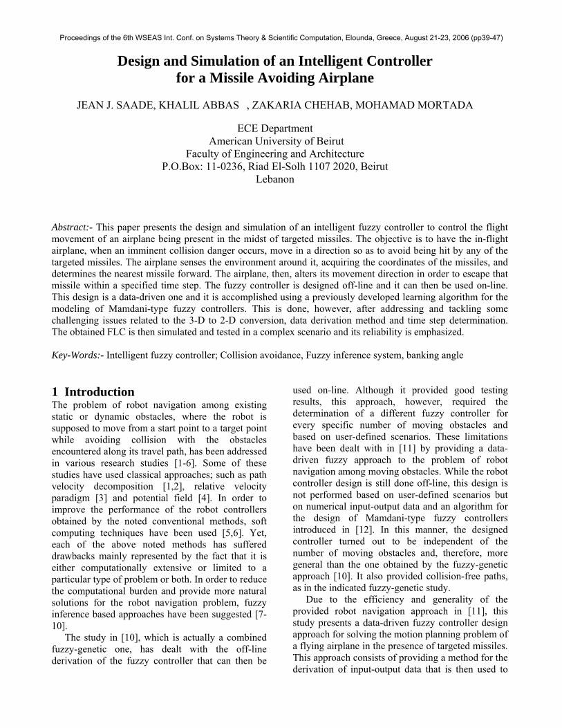
Data Acquisition Time: The round trip time that a signal takes to reach the targeting missile and bounce back to the radar present on the airplane in order to acquire the coordinates of the nearby missile. This value is obtained by dividing the double of the maximum distance between an airplane and a surrounding missile by the speed of light. The resulting time was found to be equal to 123µs. Processing Time: The time for the processor present on board the airplane to identify the (NMF) and calculate the necessary deviation it must apply in order to escape that missile. This value was estimated by comparing the time to process files of different sizes on different processors. The resulting time was taken to be: 3ms Deviation Time: The time needed for the airplane to implement the required deviation and avoid the NMF. This will be assessed based on the analysis given in Sections 3 and 4. It will be shown that the first two factors require relatively little time. The deviation time computation requires knowledge of the manner by which an airplane deviates. 3 Airplane Banking Turn Contrary to how the robot maneuvers in a 2-Dimensional plane, the airplane does not turn left and right instantaneously. Instead, it moves continuously while still in motion, which requires the airplane to turn by tilting to the side to which the deviation is intended. The angle it makes by tilting is called the banking angle. The airplane makes the necessary turn while still moving at a constant speed. Figures 1 and 2 illustrate the way an airplane turns by tilting to its side.

Figure 1. The airplane turns by tilting to its side. The airplane therefore deviates by moving on a circular trajectory that is tangential to the straight line direction on which it was initially moving. The banking angle that the airplane makes with the normal has a direct relation with the radius of the circular trajectory it follows when it deviates. In

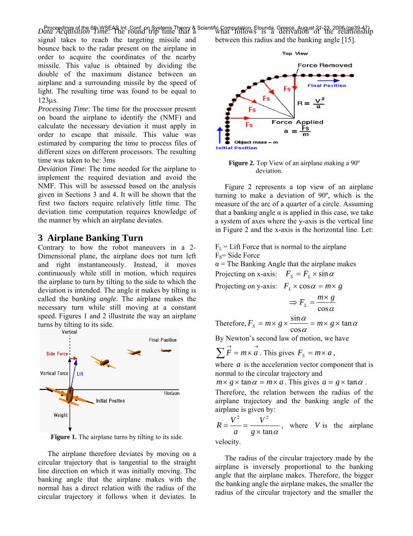
what follows is a derivation of the relationship between this radius and the banking angle [15].

Figure 2. Top View of an airplane making a 90º deviation. Figure 2 represents a top view of an airplane turning to make a deviation of 90º, which is the measure of the arc of a quarter of a circle. Assuming that a banking angle α is applied in this case, we take a system of axes where the y-axis is the vertical line in Figure 2 and the x-axis is the horizontal line. Let: FL = Lift Force that is normal to the airplane FS= Side Force α = The Banking Angle that the airplane makes Projecting on x-axis: αsin×= LS FF Projecting on y-axis: gmFL ×=× αcos

αcosgmFL

×=⇒

Therefore, ααα tan

cossin

××=××= gmgmFS

By Newton’s second law of motion, we have →→

×=∑ amF . This gives , amFS ×=where is the acceleration vector component that is normal to the circular trajectory and

a

amgm ×=×× αtan . This gives αtan×= ga . Therefore, the relation between the radius of the airplane trajectory and the banking angle of the airplane is given by:

αtan

22

×==

gV

aVR , where V is the airplane

velocity. The radius of the circular trajectory made by the airplane is inversely proportional to the banking angle that the airplane makes. Therefore, the bigger the banking angle the airplane makes, the smaller the radius of the circular trajectory and the smaller the

Proceedings of the 6th WSEAS Int. Conf. on Systems Theory & Scientific Computation, Elounda, Greece, August 21-23, 2006 (pp39-47)

distance that the airplane has to make in order to reach a certain angle. Different airplane types have different capabilities. For example, the Airbus A320 makes a maximum banking angle of 67 degrees. Similar commercial airliners have comparable banking capacities. It is for this purpose that we opted for a more agile airplane for our design; with maximum banking angle capability of 89º, which allows the airplane to move at a circular trajectory of minimum radius 1.28686 Km. A military airplane has the ability to make a banking angle of 90º. This angle though, does not result in any deviation since a zero radius would be obtained. The conclusion to draw from the relation obtained above is that with a larger radius (i.e. smaller banking angle), an airplane can achieve the same deviation angle as with a small radius. The difference though lies in the fact that a greater distance, and consequently greater time, must be covered with the large radius in order to achieve that same deviation. This fact plays a decisive role in the calculation of the time step of the controller and an equally important role in the algorithm or decision process as will be shown in the following sections. 4 Deviation Time From the material presented in Section 3, we are now able to deduce the value of the deviation time, which is the amount of time required by the plane to make the deviation dictated by the controller in order to avoid collision with the NMF. The deviation of an airplane as previously illustrated occurs by moving on a circular trajectory of radius related to the airplane banking angle. An airplane can therefore embark on a circular trajectory of whichever allowable radius in order to deviate by a certain arc measure.

The calculation of the deviation time, and consequently the time step, T, is subject to opposing limits. The lower limit states that any chosen deviation time must be enough for the airplane to make the maximum possible deviation required from it. The allotted deviation time must therefore be sufficient for the airplane to be able to make this kind of deviation.

The upper limit on the time step states that this recurring time interval must be minimal in order for the controller to be able to handle the maximum possible number of missiles in the least time possible. Having the Time Step very large would result in undesired consequences as it would take a long time for the airplane to escape a single missile leaving ample time for other surrounding missiles,

other than the (NMF), to approach the airplane or even possibly colliding with it. As in the case of a robot in a 2-dimensional environment, the airplane maximum deviation is 90°, occurring almost exclusively when the approaching missile circular cut with the flight plane is extremely close or is engulfing the position of the airplane. This implies that a deviation of 90° is required only when the airplane is moving on its minimal radius. The time needed for this 90° deviation to take place at the minimum radius (i.e. maximum banking angle) is equal to 2.378 seconds.

The cumulative time interval that constitutes the time step T is therefore estimated to be 3 seconds. We note here that some large angles to be made on circular trajectories with larger radii than the minimum radius may need more time than the allocated 3 seconds. This will be taken care of in the safety margin analysis given in Section 6. 5 Three Dimensional/Two Dimensional Mapping Taking into account the values adopted at the start of this analysis, an airplane traveling at constant speed moves a distance of 850T meters in one time step, T. During this time interval, the targeting missile would have traveled 1000T meters. The direction in which the missile moves in its 3-dimensional space is unknown. The possible positions that a missile occupies in one time step could, therefore, be represented by a sphere of radius 1000T. The decision as to whether the missile surrounding an airplane poses an eminent threat on which the airplane must deviate depends first of all on whether the sphere of the missile intersects with the plane on which the targeted airplane is traveling.

The intersection, whenever it occurs, between the flight plane and the sphere whose radius is equal to the distance traveled by the missile in time T results in a circle. In our analysis we assume that the radar located at the plane is the center of the coordinate system. This installed radar gives us the spherical coordinates of the missile (r,θ ,φ ).

Now, in order to facilitate our analysis we transform the spherical coordinates obtained by the radar to Cartesian coordinates:

θφ sincos ××= ra , θφ sinsin ××= rb ,

θcos×= rc . The equation of the sphere of the missile in one time step is: ( ) ( ) ( ) 2222

SRczbyax =−+−+− where the radius of the sphere, RS, is equal to 1000T.

Proceedings of the 6th WSEAS Int. Conf. on Systems Theory & Scientific Computation, Elounda, Greece, August 21-23, 2006 (pp39-47)

The plane of flight is the x-y plane has the equation . The intersection between the sphere and the plane equations yields:

0=z

( ) ( ) 2222 )0( SRcbyax =−+−+− . This gives

( ) ( ) )( 22S

22 cRbyax −=−+− . Hence, the intersection is a circle with center (a,b) and radius:

)( 22 cRr Sc −= . The radius of the circle rc depends on the altitude

c. At c=0 we have rc=Rs and the circle will have a maximum value i.e. the intersection will occur at the center of the sphere. As c increases, the intersection would move further from the center of the sphere towards the extremity and hence rc decreases accordingly.

The outcome of this analysis is the mapping of the 3-dimensional problem into a manageable 2-dimensional one that can be handled in the following manner. A missile is judged eminently dangerous if its representing sphere first intersects with the flight plane and second intersects with the line segment that the airplane would travel in that plane of flight in T seconds. If more than one missile fulfills this condition, then the one considered closer to the current position of the airplane is regarded as the NMF. Upon locating the circle representing the NMF, the airplane controller will then decide on the appropriate deviation and execute it. Next we consider a case study to better explain the noted ideas and how the necessary deviation is determined.

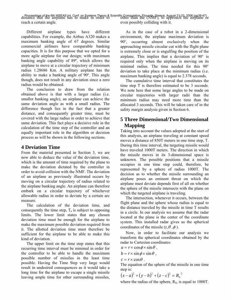
6 Safety Margin analysis We consider the case of an approaching missile of Cartesian coordinates (0,4.5,2) in Km. The missile is represented be a sphere of radius 1000T= 3km. The intersection of this sphere with the flight plane is represented by a circle of coordinates (0,4.5) and radius 2.236 Km. The missile is clearly intersecting with the trajectory of the airplane that is represented by the traveled line segment on the y-axis of length 2.55Km (Figure 3). Therefore a deviation from the initial trajectory of the airplane is in order.

As Figure 3 shows, the deviation occurs by creating the banking angle corresponding to the circle tangential to the one representing the missile. The figure also reveals that the distance that the airplane needs to cover in order to reach the point tangential to the missile circle is 3.1542 Km, which can not be covered in one time step since the airplane can only travel a distance of 2.55 Km in 3 seconds. This leaves the airplane 0.6042 Km short from the safety point since it reaches a position where it would be in danger of collision with the missile in the next 3-second time step.

Figure 3. AutoCAD plot representing the deviation

trajectory of an airplane.

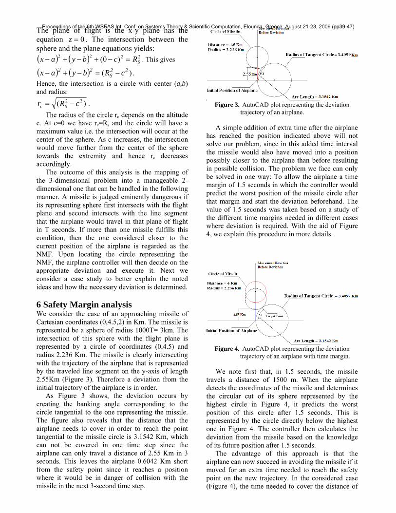
A simple addition of extra time after the airplane has reached the position indicated above will not solve our problem, since in this added time interval the missile would also have moved into a position possibly closer to the airplane than before resulting in possible collision. The problem we face can only be solved in one way: To allow the airplane a time margin of 1.5 seconds in which the controller would predict the worst position of the missile circle after that margin and start the deviation beforehand. The value of 1.5 seconds was taken based on a study of the different time margins needed in different cases where deviation is required. With the aid of Figure 4, we explain this procedure in more details.

Figure 4. AutoCAD plot representing the deviation trajectory of an airplane with time margin.

We note first that, in 1.5 seconds, the missile

travels a distance of 1500 m. When the airplane detects the coordinates of the missile and determines the circular cut of its sphere represented by the highest circle in Figure 4, it predicts the worst position of this circle after 1.5 seconds. This is represented by the circle directly below the highest one in Figure 4. The controller then calculates the deviation from the missile based on the knowledge of its future position after 1.5 seconds.

The advantage of this approach is that the airplane can now succeed in avoiding the missile if it moved for an extra time needed to reach the safety point on the new trajectory. In the considered case (Figure 4), the time needed to cover the distance of

Proceedings of the 6th WSEAS Int. Conf. on Systems Theory & Scientific Computation, Elounda, Greece, August 21-23, 2006 (pp39-47)

3.1542 Km between the position of the airplane and the safety point is in fact less than the allocated 4.5 seconds. The 4.5 seconds is the maximum time within which all cases can be accommodated.

We note here that the circular cut radius, rc, and the length of the line segment traveled by the airplane in a time step are still to be calculated based on 3 seconds. The extra 1.5 seconds are only used to determine the predicted worst position of the circular cut and on the basis of which we obtain the necessary deviation. 7 FLC Design After addressing and resolving the challenges of the problem, numerical input-output data representing a good number of missiles positions and their required deviation angles are obtained. These data can then be used to construct a fuzzy logic controller whose role is to provide the airplane with the required banking angle to avoid being hit by a missile.

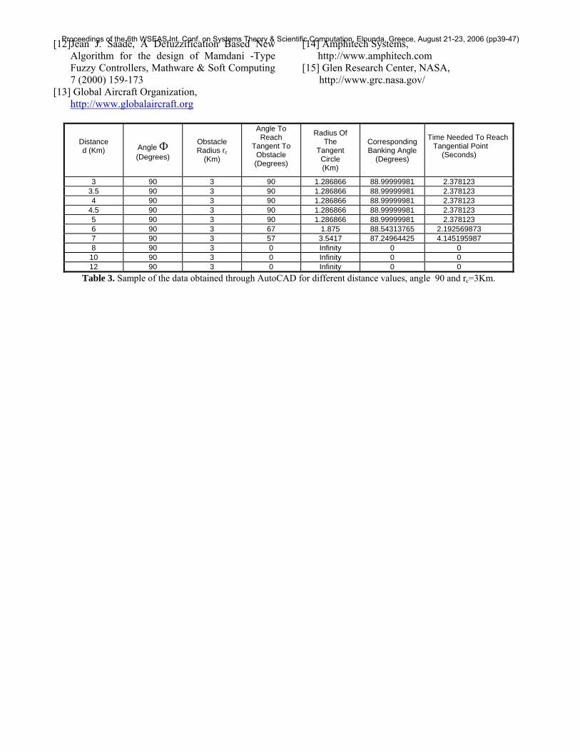
With the aid of AutoCAD, we have collected the data necessary in order to construct the FLC by computing the different banking angles required for many missile positions. The data acquired was distributed in a grid-like fashion so as to have as many as possible cases of missile positions covered. Also, more values have been collected at positions where the missiles were extremely close to the airplane as these cases are more critical than others and therefore require more accuracy. The table at the end of this paper shows a sample of the obtained data.

The data points collected have been used to construct a Mamdani’s type fuzzy logic controller with the help of [2]. This controller design methodology has the ability to learn the rules of the fuzzy system form the provided data. The 3 inputs of the FLC are the distance, the angle and the radius in the 2D plane. The distance input is denoted by d and it is the length measure from the airplane sensor to the center of the circular cut of the sphere surrounding the missile position with the plane of

flight. d is therefore given by ( ) θsin22 rba =+ . The angle Ф is taken as the angle between the

direction perpendicular to the airplane flight (y-direction) and straight line joining the sensor position (airplane) and the center of the circular cut of the missile sphere with the plane of flight. Hence, Ф = φ . As for the radius, it is symbolized by rc (refer to Section 3) and it varies according to the altitude component c. It is to be noted here that the formulas for d, Ф, and rc are only applicable when the sphere surrounding the missile position and of radius Rs has a circular cut with the plane of flight. That is, when Rsrc <= θcos . If this condition is

not satisfied for any of sensor detected missiles, then the system will consider this case as if there are no missiles and therefore no alternation of the flight direction will be necessary.

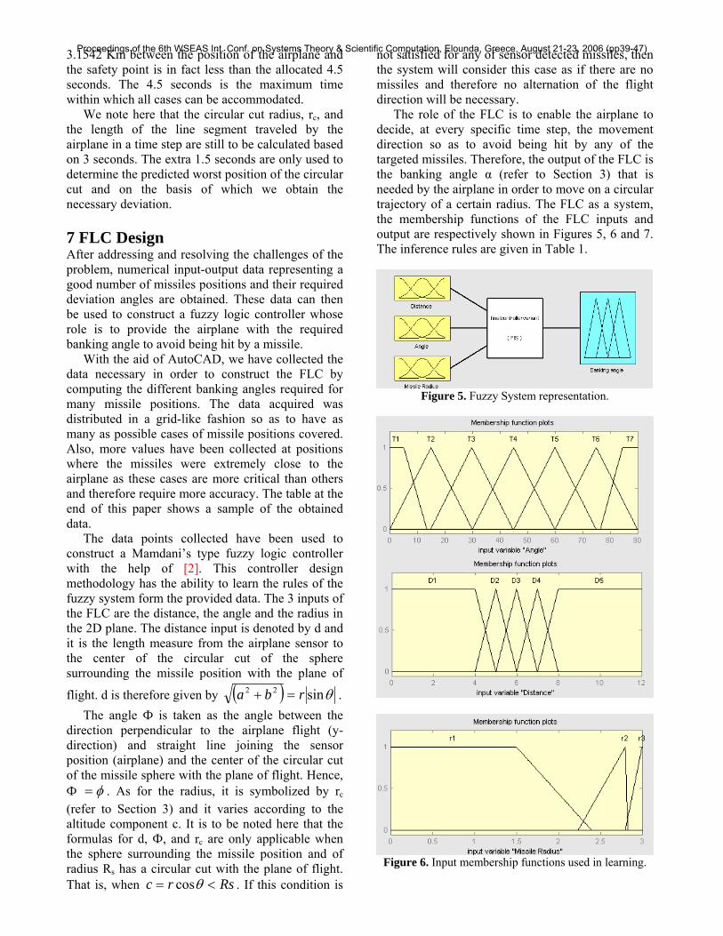
The role of the FLC is to enable the airplane to decide, at every specific time step, the movement direction so as to avoid being hit by any of the targeted missiles. Therefore, the output of the FLC is the banking angle α (refer to Section 3) that is needed by the airplane in order to move on a circular trajectory of a certain radius. The FLC as a system, the membership functions of the FLC inputs and output are respectively shown in Figures 5, 6 and 7. The inference rules are given in Table 1.

Figure 5. Fuzzy System representation.

Figure 6. Input membership functions used in learning.

Proceedings of the 6th WSEAS Int. Conf. on Systems Theory & Scientific Computation, Elounda, Greece, August 21-23, 2006 (pp39-47)

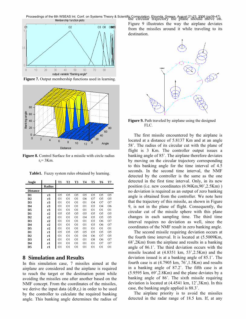
Figure 7. Output membership functions used in learning.

Figure 8. Control Surface for a missile with circle radius rc= 3Km.

Table1. Fuzzy system rules obtained by learning.

Angle T1 T2 T3 T4 T5 T6 T7 Radius Distance D1 r3 O5 O5 O5 O5 O5 O5 O5 D2 r3 O1 O1 O1 O6 O7 O5 O5 D3 r3 O1 O1 O1 O1 O4 O7 O7 D4 r3 O1 O1 O1 O1 O3 O4 O6 D5 r3 O1 O1 O1 O1 O1 O1 O1 D1 r2 O5 O5 O5 O5 O5 O5 O5 D2 r2 O1 O1 O1 O4 O5 O5 O5 D3 r2 O1 O1 O1 O1 O3 O6 O7 D4 r2 O1 O1 O1 O1 O3 O6 O7 D5 r2 O1 O1 O1 O1 O1 O1 O1 D1 r1 O5 O5 O5 O5 O5 O5 O5 D2 r1 O1 O1 O1 O4 O6 O7 O5 D3 r1 O1 O1 O1 O1 O8 O6 O7 D4 r1 O1 O1 O1 O1 O1 O7 O7 D5 r1 O1 O1 O1 O1 O1 O1 O1

8 Simulation and Results In this simulation case, 7 missiles aimed at the airplane are considered and the airplane is required to reach the target or the destination point while avoiding the missiles one after another based on the NMF concept. From the coordinates of the missiles, we derive the input data (d,Ф,rc) in order to be used by the controller to calculate the required banking angle. This banking angle determines the radius of

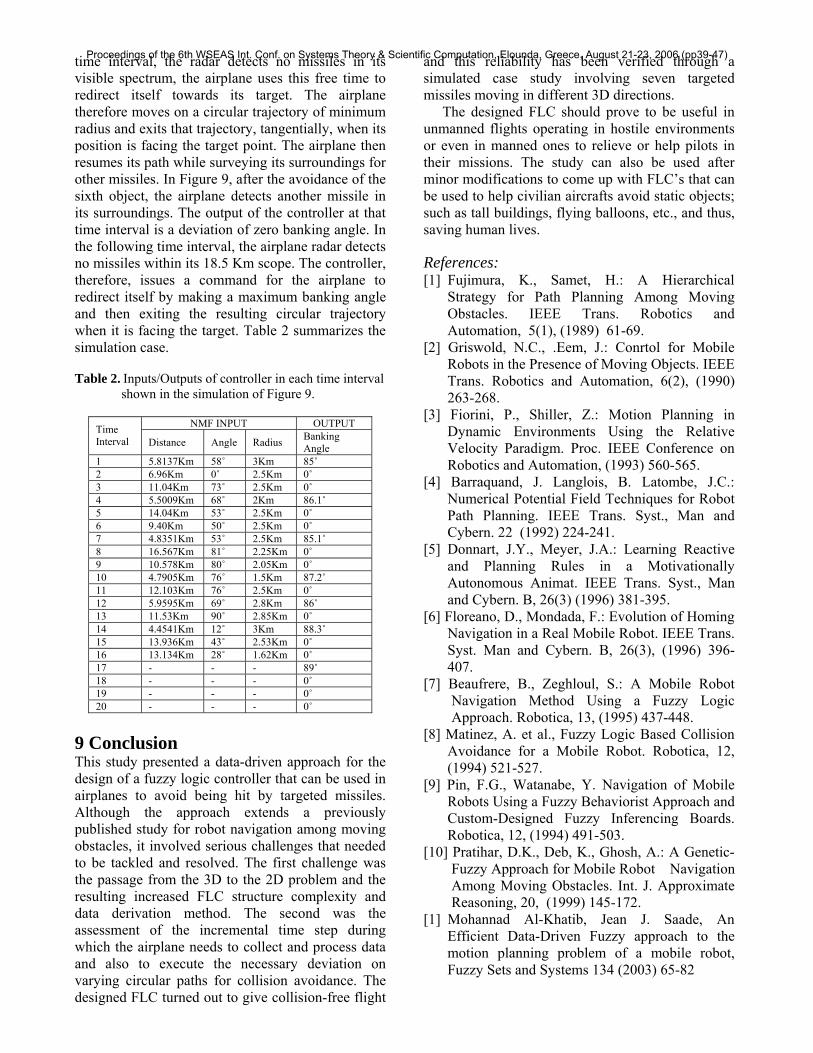
the circular trajectory the plane should move on. Figure 9 illustrates the way the airplane deviates from the missiles around it while traveling to its destination.

Figure 9. Path traveled by airplane using the designed FLC.

The first missile encountered by the airplane is located at a distance of 5.8137 Km and at an angle 58˚. The radius of its circular cut with the plane of flight is 3 Km. The controller output issues a banking angle of 85˚. The airplane therefore deviates by moving on the circular trajectory corresponding to this banking angle for the time interval of 4.5 seconds. In the second time interval, the NMF detected by the controller is the same as the one detected in the first time interval. Only, in its new position (i.e. new coordinates (6.96Km,90˚,2.5Km) ) no deviation is required as an output of zero banking angle is obtained from the controller. We note here that the trajectory of this missile, as shown in Figure 9, is not in the plane of flight. Consequently, the circular cut of the missile sphere with this plane changes in each sampling time. The third time interval requires no deviation as well, since the coordinates of the NMF result in zero banking angle.

The second missile requiring deviation occurs at the fourth time interval. It is located at (5.5009Km, 68˚,2Km) from the airplane and results in a banking angle of 86.1˚. The third deviation occurs with the missile located at (4.8351 km, 53˚,2.5Km) and the deviation issued is at a banking angle of 85.1˚. The fourth case is at (4.7905 km, 76˚,1.5Km) and results in a banking angle of 87.2˚. The fifth case is at (5.9595 km, 69˚,2.8Km) and the plane deviates by a banking angle of 86˚. The sixth missile requiring deviation is located at (4.4541 km, 12˚,3Km). In this case, the banking angle applied is 88.3˚.

The airplane priority is to avoid the missiles detected in the radar range of 18.5 km. If, at any

Proceedings of the 6th WSEAS Int. Conf. on Systems Theory & Scientific Computation, Elounda, Greece, August 21-23, 2006 (pp39-47)

time interval, the radar detects no missiles in its visible spectrum, the airplane uses this free time to redirect itself towards its target. The airplane therefore moves on a circular trajectory of minimum radius and exits that trajectory, tangentially, when its position is facing the target point. The airplane then resumes its path while surveying its surroundings for other missiles. In Figure 9, after the avoidance of the sixth object, the airplane detects another missile in its surroundings. The output of the controller at that time interval is a deviation of zero banking angle. In the following time interval, the airplane radar detects no missiles within its 18.5 Km scope. The controller, therefore, issues a command for the airplane to redirect itself by making a maximum banking angle and then exiting the resulting circular trajectory when it is facing the target. Table 2 summarizes the simulation case. Table 2. Inputs/Outputs of controller in each time interval shown in the simulation of Figure 9.

NMF INPUT OUTPUT Time Interval Distance Angle Radius Banking

Angle 1 5.8137Km 58˚ 3Km 85˚ 2 6.96Km 0˚ 2.5Km 0˚ 3 11.04Km 73˚ 2.5Km 0˚ 4 5.5009Km 68˚ 2Km 86.1˚ 5 14.04Km 53˚ 2.5Km 0˚ 6 9.40Km 50˚ 2.5Km 0˚ 7 4.8351Km 53˚ 2.5Km 85.1˚ 8 16.567Km 81˚ 2.25Km 0˚ 9 10.578Km 80˚ 2.05Km 0˚ 10 4.7905Km 76˚ 1.5Km 87.2˚ 11 12.103Km 76˚ 2.5Km 0˚ 12 5.9595Km 69˚ 2.8Km 86˚ 13 11.53Km 90˚ 2.85Km 0˚ 14 4.4541Km 12˚ 3Km 88.3˚ 15 13.936Km 43˚ 2.53Km 0˚ 16 13.134Km 28˚ 1.62Km 0˚ 17 - - - 89˚ 18 - - - 0˚ 19 - - - 0˚ 20 - - - 0˚

9 Conclusion This study presented a data-driven approach for the design of a fuzzy logic controller that can be used in airplanes to avoid being hit by targeted missiles. Although the approach extends a previously published study for robot navigation among moving obstacles, it involved serious challenges that needed to be tackled and resolved. The first challenge was the passage from the 3D to the 2D problem and the resulting increased FLC structure complexity and data derivation method. The second was the assessment of the incremental time step during which the airplane needs to collect and process data and also to execute the necessary deviation on varying circular paths for collision avoidance. The designed FLC turned out to give collision-free flight

and this reliability has been verified through a simulated case study involving seven targeted missiles moving in different 3D directions.

The designed FLC should prove to be useful in unmanned flights operating in hostile environments or even in manned ones to relieve or help pilots in their missions. The study can also be used after minor modifications to come up with FLC’s that can be used to help civilian aircrafts avoid static objects; such as tall buildings, flying balloons, etc., and thus, saving human lives. References: [1] Fujimura, K., Samet, H.: A Hierarchical

Strategy for Path Planning Among Moving Obstacles. IEEE Trans. Robotics and Automation, 5(1), (1989) 61-69.

[2] Griswold, N.C., .Eem, J.: Conrtol for Mobile Robots in the Presence of Moving Objects. IEEE Trans. Robotics and Automation, 6(2), (1990) 263-268.

[3] Fiorini, P., Shiller, Z.: Motion Planning in Dynamic Environments Using the Relative Velocity Paradigm. Proc. IEEE Conference on Robotics and Automation, (1993) 560-565.

[4] Barraquand, J. Langlois, B. Latombe, J.C.: Numerical Potential Field Techniques for Robot Path Planning. IEEE Trans. Syst., Man and Cybern. 22 (1992) 224-241.

[5] Donnart, J.Y., Meyer, J.A.: Learning Reactive and Planning Rules in a Motivationally Autonomous Animat. IEEE Trans. Syst., Man and Cybern. B, 26(3) (1996) 381-395.

[6] Floreano, D., Mondada, F.: Evolution of Homing Navigation in a Real Mobile Robot. IEEE Trans. Syst. Man and Cybern. B, 26(3), (1996) 396-407.

[7] Beaufrere, B., Zeghloul, S.: A Mobile Robot Navigation Method Using a Fuzzy Logic Approach. Robotica, 13, (1995) 437-448.

[8] Matinez, A. et al., Fuzzy Logic Based Collision Avoidance for a Mobile Robot. Robotica, 12, (1994) 521-527.

[9] Pin, F.G., Watanabe, Y. Navigation of Mobile Robots Using a Fuzzy Behaviorist Approach and Custom-Designed Fuzzy Inferencing Boards. Robotica, 12, (1994) 491-503.

[10] Pratihar, D.K., Deb, K., Ghosh, A.: A Genetic-Fuzzy Approach for Mobile Robot Navigation Among Moving Obstacles. Int. J. Approximate Reasoning, 20, (1999) 145-172.

[1] Mohannad Al-Khatib, Jean J. Saade, An Efficient Data-Driven Fuzzy approach to the motion planning problem of a mobile robot, Fuzzy Sets and Systems 134 (2003) 65-82

Proceedings of the 6th WSEAS Int. Conf. on Systems Theory & Scientific Computation, Elounda, Greece, August 21-23, 2006 (pp39-47)

[12]Jean J. Saade, A Defuzzification Based New Algorithm for the design of Mamdani -Type Fuzzy Controllers, Mathware & Soft Computing 7 (2000) 159-173

[13] Global Aircraft Organization, http://www.globalaircraft.org

[14] Amphitech Systems, http://www.amphitech.com [15] Glen Research Center, NASA,

http://www.grc.nasa.gov/

Distance d (Km)

Angle Ф (Degrees)

Obstacle Radius rc

(Km)

Angle To Reach

Tangent To Obstacle (Degrees)

Radius Of The

Tangent Circle (Km)

Corresponding Banking Angle

(Degrees)

Time Needed To Reach Tangential Point

(Seconds)

3 90 3 90 1.286866 88.99999981 2.378123 3.5 90 3 90 1.286866 88.99999981 2.378123 4 90 3 90 1.286866 88.99999981 2.378123

4.5 90 3 90 1.286866 88.99999981 2.378123 5 90 3 90 1.286866 88.99999981 2.378123 6 90 3 67 1.875 88.54313765 2.192569873 7 90 3 57 3.5417 87.24964425 4.145195987 8 90 3 0 Infinity 0 0

10 90 3 0 Infinity 0 0 12 90 3 0 Infinity 0 0

Table 3. Sample of the data obtained through AutoCAD for different distance values, angle 90 and rc=3Km.

Proceedings of the 6th WSEAS Int. Conf. on Systems Theory & Scientific Computation, Elounda, Greece, August 21-23, 2006 (pp39-47)