
16 — Parallel Performance Analysis and Profiling — 1616-1
Performance Analysis[16] Slide 1 Höchstleistungsrechenzentrum Stuttgart
Parallel Performance Analysisand
Profiling
Rolf Rabenseifner
University of StuttgartHigh-Performance Computing-Center Stuttgart (HLRS)
www.hlrs.de
Parallel P
erformance A
nalysis and Profiling [16]
Rolf RabenseifnerPerformance Analysis[16] Slide 2 / 42 Höchstleistungsrechenzentrum Stuttgart
Goals of Parallel Performance Analysis
• Find performance bottlenecks• Measure parallelization overhead• Try to understand speedup value• Verification of parallel execution
Goals of this lecture
• To give an impression of the tools
– Helpful features
– Ease of use
16 — Parallel Performance Analysis and Profiling — 1616-2
Rolf RabenseifnerPerformance Analysis[16] Slide 3 / 42 Höchstleistungsrechenzentrum Stuttgart
Outline
slide no.
• Principles of performance analysis 4
• Visualization examples with Vampir NG 13
• Paraver 22
• KOJAK / Expert 23
• Most simple counter profiling 36
• Summary 41
• Technical appendix 38
Acknowledgments
• Andreas Knüpfer, ZIH – insight to Vampir NG• Claudia Schmidt, ZIH – first slides on Vampir• Rainer Keller, HLRS – background information on Paraver• Bernd Mohr, Felix Wolf – access to KOJAK/Expert
Parallel P
erformance A
nalysis and Profiling [16]
Rolf RabenseifnerPerformance Analysis[16] Slide 4 / 42 Höchstleistungsrechenzentrum Stuttgart
Analysis Scheme
• Instrumentation of – Source code– Libraries– Executable
with probes
• Parallel execution of the in instrumented executable
• Probes write on a file:– Trace recordsand/or– Profiling information (i.e., statistical summaries)
• Analysis-tools – to read the (binary) trace/profiling information
call __trace_function_enter("sub_x");call sub_x(arg1, arg2, ...);call __trace_function_leave("sub_x");
Prin
cipl
es
16 — Parallel Performance Analysis and Profiling — 1616-3
Rolf RabenseifnerPerformance Analysis[16] Slide 5 / 42 Höchstleistungsrechenzentrum Stuttgart
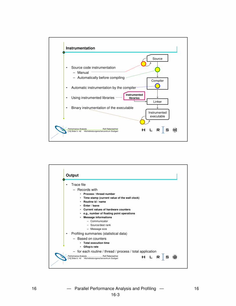
Instrumentation
• Source code instrumentation– Manual– Automatically before compiling
• Automatic instrumentation by the compiler
• Using instrumented libraries
• Binary instrumentation of the executable
Source
Compiler
Linker
instrumentedlibraries
Instrumentedexecutable
Rolf RabenseifnerPerformance Analysis[16] Slide 6 / 42 Höchstleistungsrechenzentrum Stuttgart
Output
• Trace file– Records with
• Process / thread number• Time stamp (current value of the wall clock)• Routine id / name• Enter / leave• Current values of hardware counters • e.g., number of floating point operations• Message informations
– Communicator– Source/dest rank– Message size
• Profiling summaries (statistical data)– Based on counters
• Total execution time • Gflop/s rate
– for each routine / thread / process / total application
16 — Parallel Performance Analysis and Profiling — 1616-4
Rolf RabenseifnerPerformance Analysis[16] Slide 7 / 42 Höchstleistungsrechenzentrum Stuttgart
Trace generation & Trace analysis
• E.g., with VAMPIRtraceand VAMPIR
• VAMPIRtrace must be linked with the user’sMPI application
• VAMPIRtrace writes atrace file
• VAMPIR is the graphicaltool to analyze the trace file
• VAMPIR may run – locally, or– via X window
parallel platform
user’s workstation
instrumentedapplication
VAMPIRtrace
PMPI library
Trace file
X11
user’s workstation
vampir
vampir
Server, e.g., front-end of
parallel platform
Rolf RabenseifnerPerformance Analysis[16] Slide 8 / 42 Höchstleistungsrechenzentrum Stuttgart
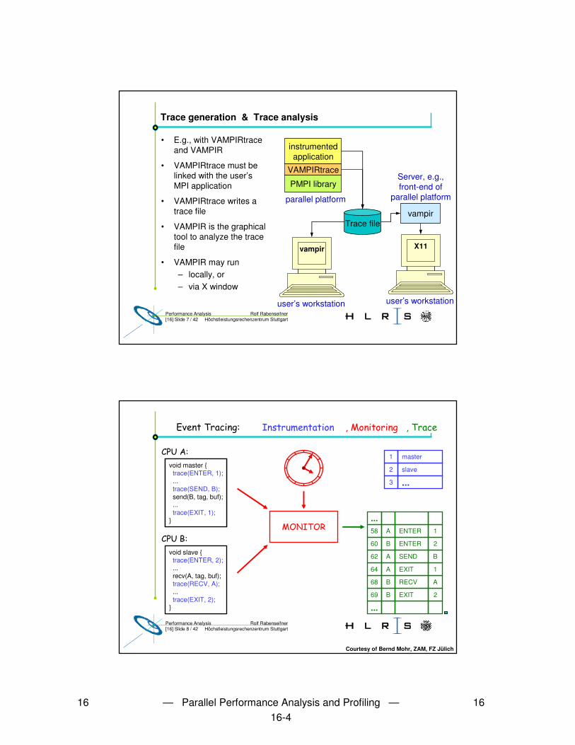
Event Tracing: Instrumentation, Monitoring, Trace
void master {
...
send(B, tag, buf);...
}
������
void slave {
...recv(A, tag, buf);
...
}
������
1 master
2 slave
3 ...
void slave {trace(ENTER, 2);...recv(A, tag, buf);trace(RECV, A);...trace(EXIT, 2);
}
void master {trace(ENTER, 1);...trace(SEND, B);send(B, tag, buf);...trace(EXIT, 1);
}
��� � ������������ ������
� � � �� � �
��� �������
58 A ENTER 1
60 B ENTER 2
62 A SEND B
64 A EXIT 1
68 B RECV A
...
69 B EXIT 2
...
��� ����
Courtesy of Bernd Mohr, ZAM, FZ Jülich
16 — Parallel Performance Analysis and Profiling — 1616-5
Rolf RabenseifnerPerformance Analysis[16] Slide 9 / 42 Höchstleistungsrechenzentrum Stuttgart
Analysis of the trace files
• Visualization of the data• Human readable• Statistics• Automated analysis of bottlenecks
– Idling processes/threads– Late receive (i.e., blocking a message sender)– Late send (i.e., blocking a receiver)
• Tools, e.g.,– Vampir (trace file visualization and statisics)– Paraver (trace file visualization and statisics)– KOJAK (automated bottleneck analysis)– Intel® Trace Analyzer– OPT from Allinea Software– TAU
Rolf RabenseifnerPerformance Analysis[16] Slide 10 / 42 Höchstleistungsrechenzentrum Stuttgart
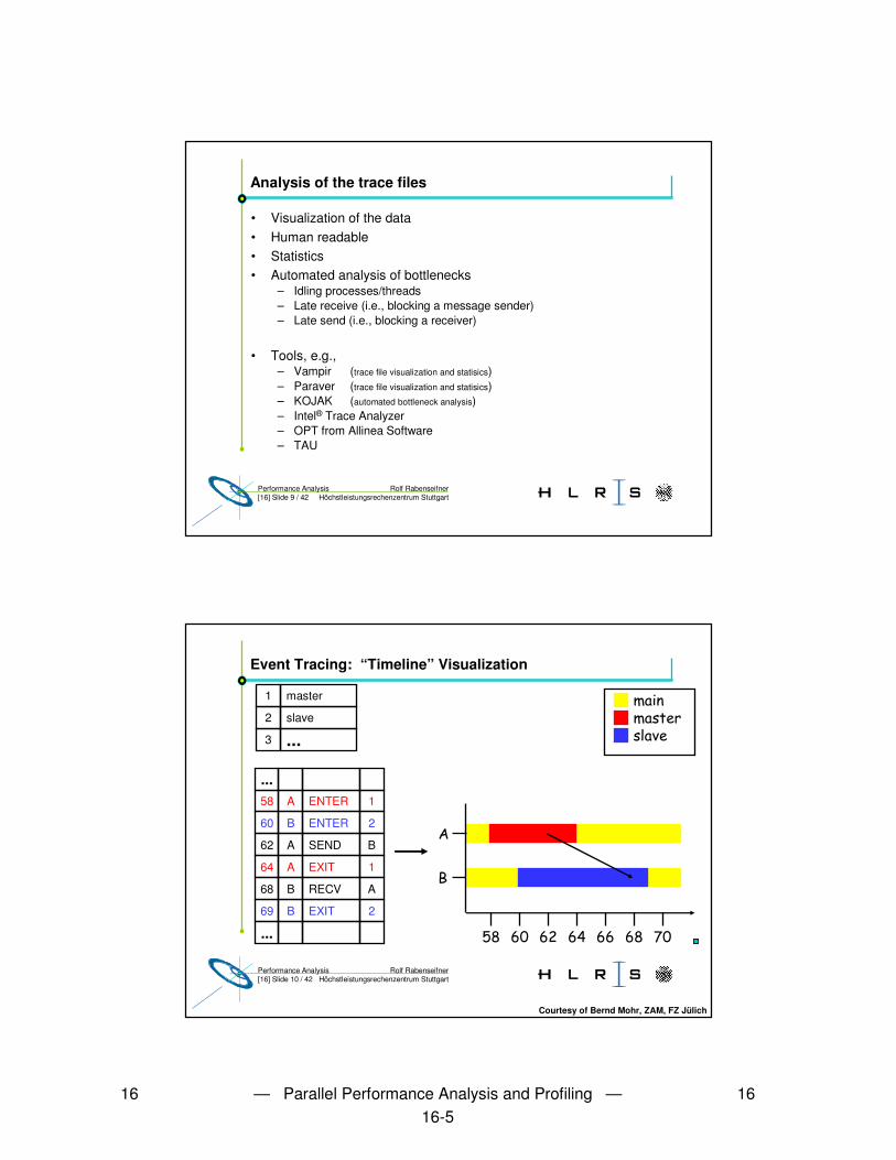
Event Tracing: “Timeline” Visualization
Courtesy of Bernd Mohr, ZAM, FZ Jülich
1 master
2 slave
3 ...
58 A ENTER 1
60 B ENTER 2
62 A SEND B
64 A EXIT 1
68 B RECV A
...
69 B EXIT 2
...
� ��� ��������
�� ! " # � $!
�
�
16 — Parallel Performance Analysis and Profiling — 1616-6
Rolf RabenseifnerPerformance Analysis[16] Slide 11 / 42 Höchstleistungsrechenzentrum Stuttgart
Rolf RabenseifnerPerformance Analysis
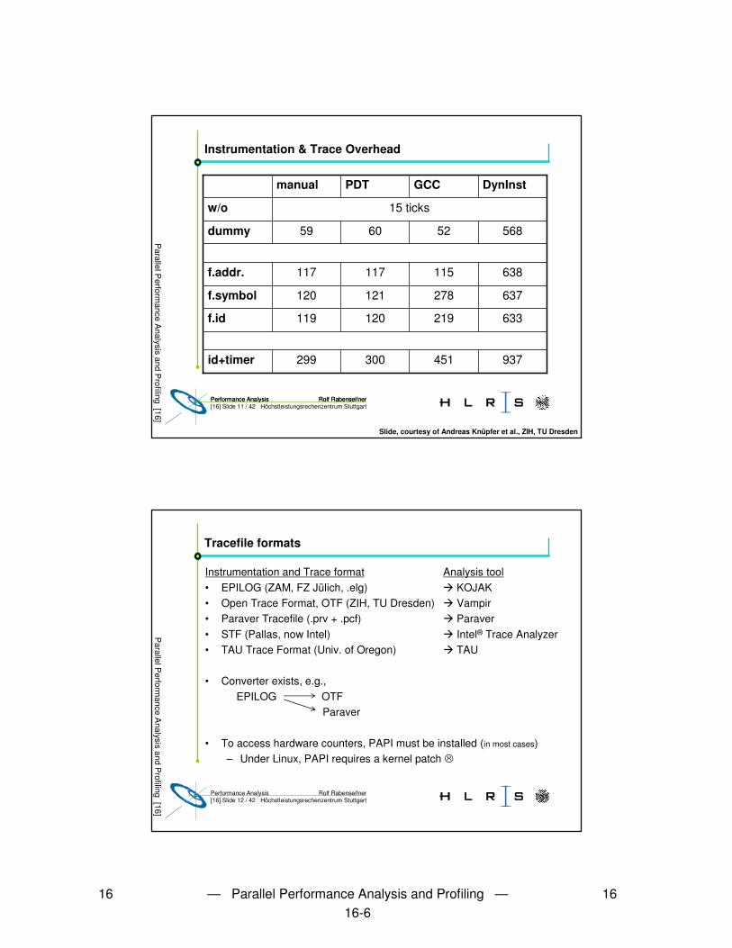
Instrumentation & Trace Overhead
Parallel P
erformance A
nalysis and Profiling [16] Slide, courtesy of Andreas Knüpfer et al., ZIH, TU Dresden
15 ticksw/o
568526059dummy
937451300299id+timer
633219120119f.id
637278121120f.symbol
638115117117f.addr.
DynInstGCCPDTmanual
Rolf RabenseifnerPerformance Analysis[16] Slide 12 / 42 Höchstleistungsrechenzentrum Stuttgart
Tracefile formats
Instrumentation and Trace format Analysis tool• EPILOG (ZAM, FZ Jülich, .elg) � KOJAK• Open Trace Format, OTF (ZIH, TU Dresden) � Vampir• Paraver Tracefile (.prv + .pcf) � Paraver• STF (Pallas, now Intel) � Intel® Trace Analyzer• TAU Trace Format (Univ. of Oregon) � TAU
• Converter exists, e.g., EPILOG OTF
Paraver
• To access hardware counters, PAPI must be installed (in most cases)– Under Linux, PAPI requires a kernel patch �
Parallel P
erformance A
nalysis and Profiling [16]
16 — Parallel Performance Analysis and Profiling — 1616-7
Rolf RabenseifnerPerformance Analysis[16] Slide 13 / 42 Höchstleistungsrechenzentrum Stuttgart
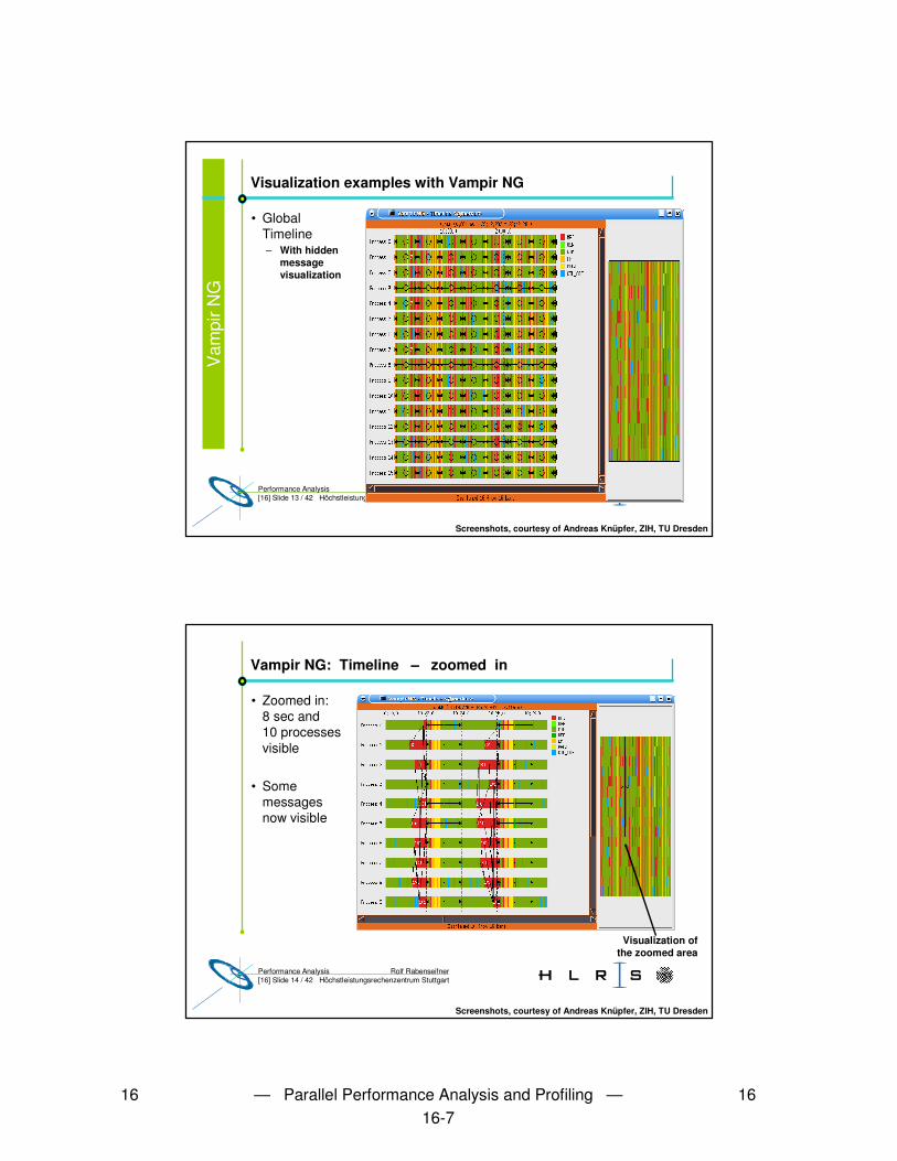
Visualization examples with Vampir NG
• GlobalTimeline– With hidden
message visualization
Screenshots, courtesy of Andreas Knüpfer, ZIH, TU Dresden
Vam
pirN
G
Rolf RabenseifnerPerformance Analysis[16] Slide 14 / 42 Höchstleistungsrechenzentrum Stuttgart
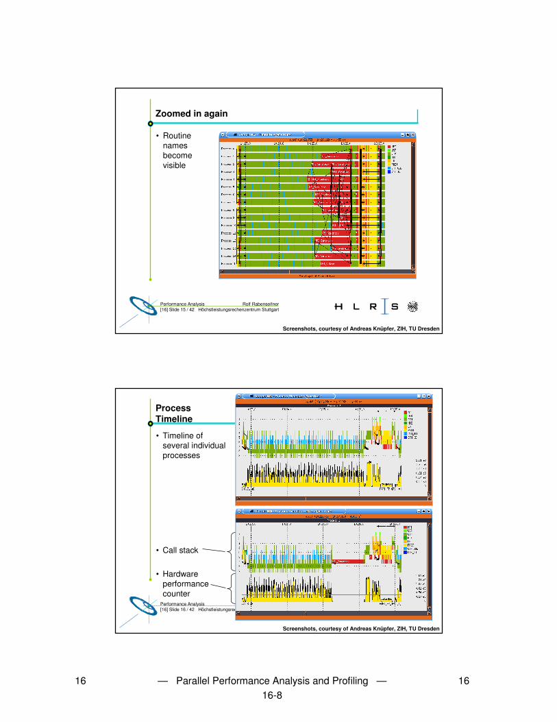
Vampir NG: Timeline – zoomed in
• Zoomed in:8 sec and 10 processes visible
• Some messages now visible
Visualization of the zoomed area
Screenshots, courtesy of Andreas Knüpfer, ZIH, TU Dresden
16 — Parallel Performance Analysis and Profiling — 1616-8
Rolf RabenseifnerPerformance Analysis[16] Slide 15 / 42 Höchstleistungsrechenzentrum Stuttgart
Zoomed in again
• Routine names become visible
Screenshots, courtesy of Andreas Knüpfer, ZIH, TU Dresden
Rolf RabenseifnerPerformance Analysis[16] Slide 16 / 42 Höchstleistungsrechenzentrum Stuttgart
ProcessTimeline
• Timeline of several individual processes
• Call stack
• Hardware performance counter
Screenshots, courtesy of Andreas Knüpfer, ZIH, TU Dresden
16 — Parallel Performance Analysis and Profiling — 1616-9
Rolf RabenseifnerPerformance Analysis[16] Slide 17 / 42 Höchstleistungsrechenzentrum Stuttgart
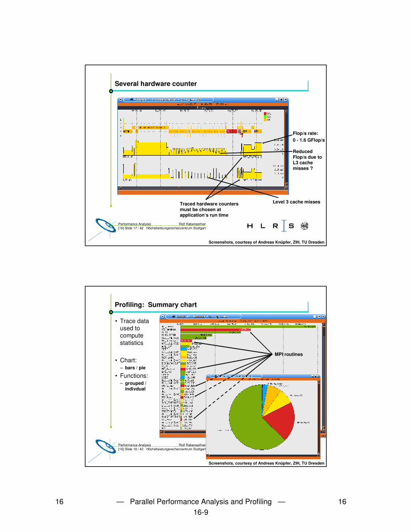
Several hardware counter
Level 3 cache misses
Flop/s rate:0 - 1.6 GFlop/s
Reduced Flop/s due to L3 cache misses ?
Traced hardware counters must be chosen at application‘s run time
Screenshots, courtesy of Andreas Knüpfer, ZIH, TU Dresden
Rolf RabenseifnerPerformance Analysis[16] Slide 18 / 42 Höchstleistungsrechenzentrum Stuttgart
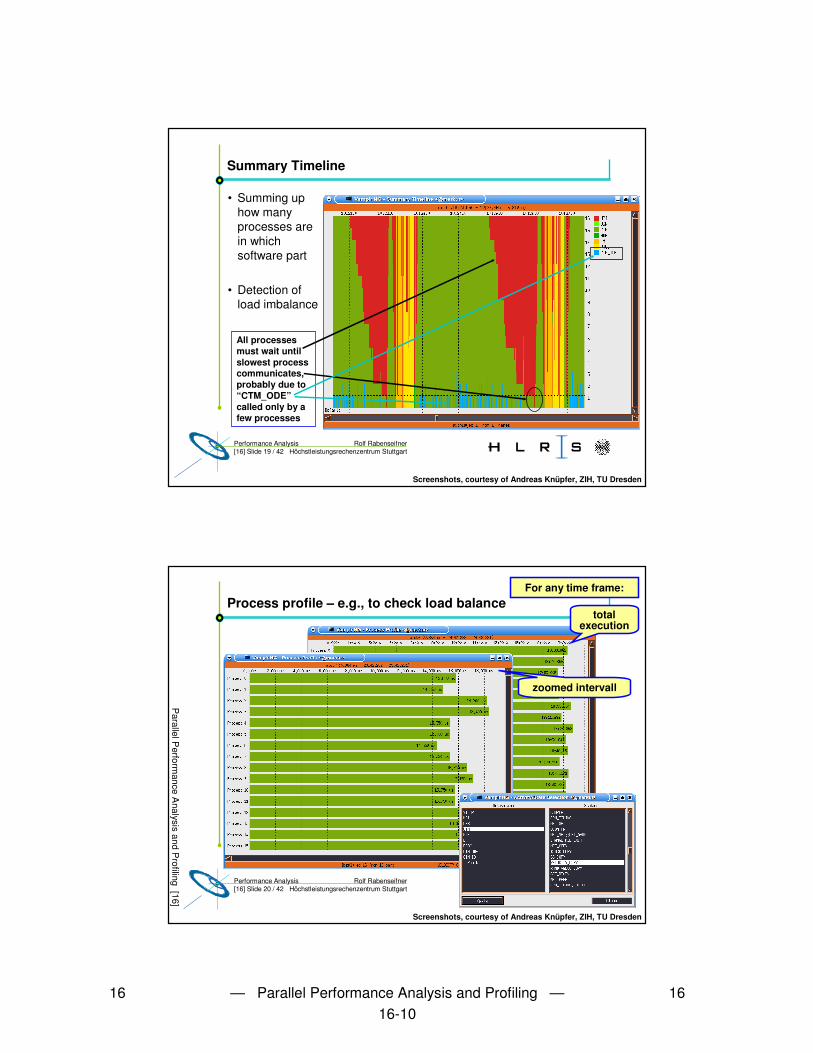
Profiling: Summary chart
• Trace data used to compute statistics
• Chart:– bars / pie
• Functions: – grouped /
indivdual
MPI routines
MPI
Screenshots, courtesy of Andreas Knüpfer, ZIH, TU Dresden
16 — Parallel Performance Analysis and Profiling — 1616-10
Rolf RabenseifnerPerformance Analysis[16] Slide 19 / 42 Höchstleistungsrechenzentrum Stuttgart
Summary Timeline
• Summing up how many processes are in which software part
• Detection of load imbalance
All processes must wait until slowest process communicates,probably due to“CTM_ODE”called only by a few processes
Screenshots, courtesy of Andreas Knüpfer, ZIH, TU Dresden
Rolf RabenseifnerPerformance Analysis[16] Slide 20 / 42 Höchstleistungsrechenzentrum Stuttgart
Process profile – e.g., to check load balance For any time frame:
total execution
zoomed intervall
Screenshots, courtesy of Andreas Knüpfer, ZIH, TU Dresden
Parallel P
erformance A
nalysis and Profiling [16]
16 — Parallel Performance Analysis and Profiling — 1616-11
Rolf RabenseifnerPerformance Analysis[16] Slide 21 / 42 Höchstleistungsrechenzentrum Stuttgart
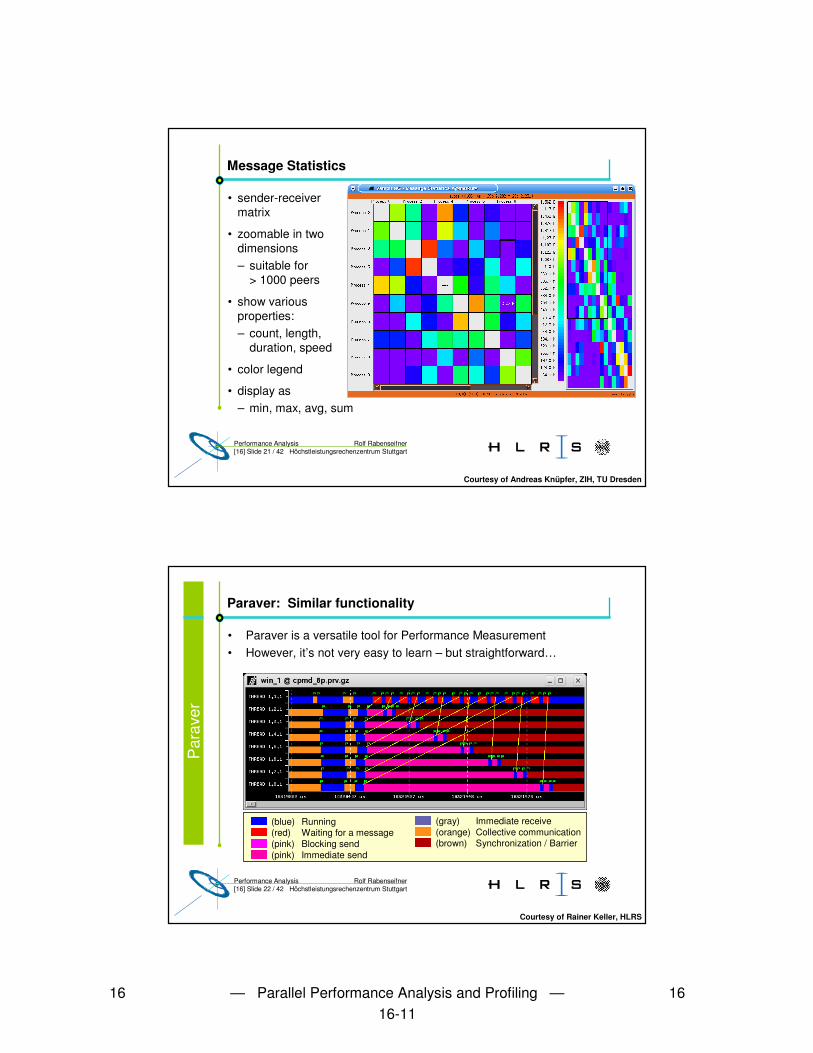
Message Statistics
• sender-receiver matrix
• zoomable in two dimensions– suitable for
> 1000 peers
• show various properties:– count, length,
duration, speed
• color legend
• display as– min, max, avg, sum
Courtesy of Andreas Knüpfer, ZIH, TU Dresden
Rolf RabenseifnerPerformance Analysis[16] Slide 22 / 42 Höchstleistungsrechenzentrum Stuttgart
Paraver: Similar functionality
• Paraver is a versatile tool for Performance Measurement• However, it’s not very easy to learn – but straightforward…
(blue) Running(red) Waiting for a message(pink) Blocking send(pink) Immediate send
(gray) Immediate receive(orange) Collective communication(brown) Synchronization / Barrier
Courtesy of Rainer Keller, HLRS
Par
aver
16 — Parallel Performance Analysis and Profiling — 1616-12
Rolf RabenseifnerPerformance Analysis[16] Slide 23 / 42 Höchstleistungsrechenzentrum Stuttgart
KOJAK / Expert
Kit for Objective Judgement and Knowledge-based Detection of Performance Bottlenecks
Joint project of• Central Institute for Applied Mathematics @ Forschungszentrum Jülich• Innovative Computing Laboratory @ the University of Tennessee
Supported programming models:• MPI, OpenMP, SHMEM, and combinations thereof.
Task:• Automated search in event traces of parallel applications
for execution patterns that indicate inefficient behavior
URL: http://www.fz-juelich.de/zam/kojak/http://www.fz-juelich.de/zam/kojak/examples/
KO
JAK
/ E
xper
t
Rolf RabenseifnerPerformance Analysis[16] Slide 24 / 42 Höchstleistungsrechenzentrum Stuttgart
KOJAK / Expert: Automated detection of performance problems
Most important patterns:• MPI:
– Point-to-point message passing:• Late receiver• Late sender• Messages in wrong order
– Collective communication• Early reduce• Late broadcast• Wait at NxN• Wait at barrier
– MPI I/O• OpenMP
• Fork overhead• Wait at explicit barrier• Wait at implicit barrier• Wait for critical section• Wait for lock
16 — Parallel Performance Analysis and Profiling — 1616-13
Rolf RabenseifnerPerformance Analysis[16] Slide 25 / 42 Höchstleistungsrechenzentrum Stuttgart
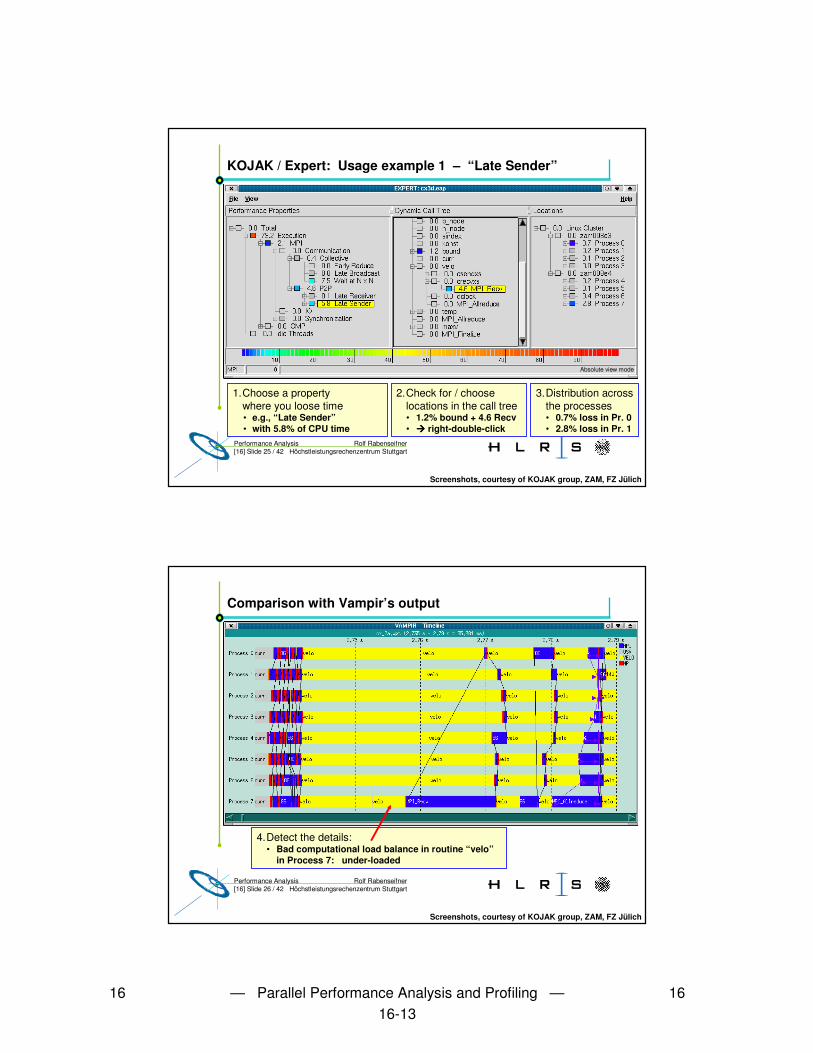
KOJAK / Expert: Usage example 1 – “Late Sender”
1.Choose a propertywhere you loose time• e.g., “Late Sender”• with 5.8% of CPU time
2.Check for / choose locations in the call tree• 1.2% bound + 4.6 Recv• ���� right-double-click
3.Distribution across the processes• 0.7% loss in Pr. 0• 2.8% loss in Pr. 1
Screenshots, courtesy of KOJAK group, ZAM, FZ Jülich
Absolute view mode
Rolf RabenseifnerPerformance Analysis[16] Slide 26 / 42 Höchstleistungsrechenzentrum Stuttgart
Comparison with Vampir’s output
4.Detect the details:• Bad computational load balance in routine “velo”
in Process 7: under-loaded
Screenshots, courtesy of KOJAK group, ZAM, FZ Jülich
16 — Parallel Performance Analysis and Profiling — 1616-14
Rolf RabenseifnerPerformance Analysis[16] Slide 27 / 42 Höchstleistungsrechenzentrum Stuttgart
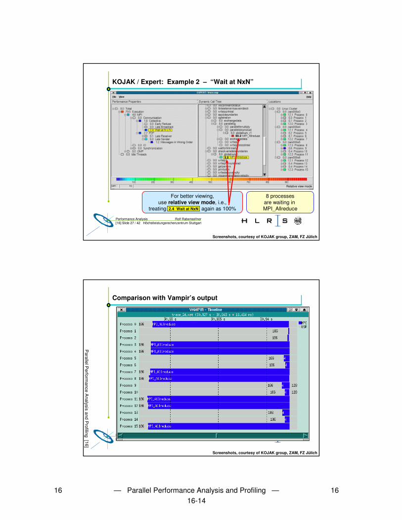
KOJAK / Expert: Example 2 – “Wait at NxN”
Screenshots, courtesy of KOJAK group, ZAM, FZ Jülich
90.2
9.8
For better viewing,use relative view mode, i.e.,
treating ___________ again as 100%2.4 Wait at NxN
8 processesare waiting in MPI_Allreduce
Relative view mode
Rolf RabenseifnerPerformance Analysis[16] Slide 28 / 42 Höchstleistungsrechenzentrum Stuttgart
Comparison with Vampir’s output
Screenshots, courtesy of KOJAK group, ZAM, FZ Jülich
Parallel P
erformance A
nalysis and Profiling [16]
16 — Parallel Performance Analysis and Profiling — 1616-15
Rolf RabenseifnerPerformance Analysis[16] Slide 29 / 42 Höchstleistungsrechenzentrum Stuttgart
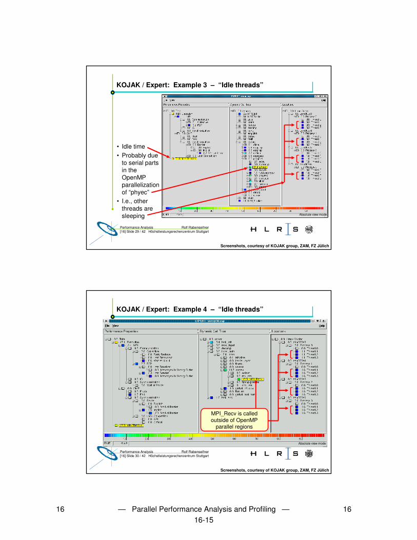
KOJAK / Expert: Example 3 – “Idle threads”
• Idle time• Probably due
to serial parts in the OpenMP parallelization of “phyec”
• I.e., other threads are sleeping
Screenshots, courtesy of KOJAK group, ZAM, FZ Jülich
Absolute view mode
Rolf RabenseifnerPerformance Analysis[16] Slide 30 / 42 Höchstleistungsrechenzentrum Stuttgart
KOJAK / Expert: Example 4 – “Idle threads”
Screenshots, courtesy of KOJAK group, ZAM, FZ Jülich
MPI_Recv is called outside of OpenMP
parallel regions
Absolute view mode
16 — Parallel Performance Analysis and Profiling — 1616-16
Rolf RabenseifnerPerformance Analysis[16] Slide 31 / 42 Höchstleistungsrechenzentrum Stuttgart
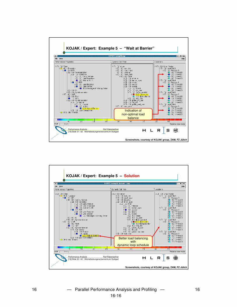
KOJAK / Expert: Example 5 – “Wait at Barrier”
Screenshots, courtesy of KOJAK group, ZAM, FZ Jülich
Relative view mode
Indication of non-optimal load
balance
Rolf RabenseifnerPerformance Analysis[16] Slide 32 / 42 Höchstleistungsrechenzentrum Stuttgart
KOJAK / Expert: Example 5 – Solution
Screenshots, courtesy of KOJAK group, ZAM, FZ Jülich
Relative view mode
Better load balancing with
dynamic loop schedule
16 — Parallel Performance Analysis and Profiling — 1616-17
Rolf RabenseifnerPerformance Analysis[16] Slide 33 / 42 Höchstleistungsrechenzentrum Stuttgart
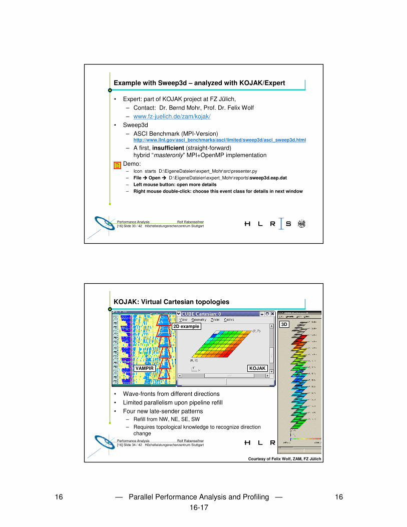
Example with Sweep3d – analyzed with KOJAK/Expert
• Expert: part of KOJAK project at FZ Jülich, – Contact: Dr. Bernd Mohr, Prof. Dr. Felix Wolf– www.fz-juelich.de/zam/kojak/
• Sweep3d– ASCI Benchmark (MPI-Version)
http://www.llnl.gov/asci_benchmarks/asci/limited/sweep3d/asci_sweep3d.html
– A first, insufficient (straight-forward) hybrid “masteronly” MPI+OpenMP implementation
• Demo:– Icon starts D:\EigeneDateien\expert_Mohr\src\presenter.py– File ���� Open ���� D:\EigeneDateien\expert_Mohr\reports\sweep3d.eap.dat– Left mouse button: open more details– Right mouse double-click: choose this event class for details in next window
Rolf RabenseifnerPerformance Analysis[16] Slide 34 / 42 Höchstleistungsrechenzentrum Stuttgart
KOJAK: Virtual Cartesian topologies
• Wave-fronts from different directions• Limited parallelism upon pipeline refill • Four new late-sender patterns
– Refill from NW, NE, SE, SW– Requires topological knowledge to recognize direction
change
VAMPIR
Courtesy of Felix Wolf, ZAM, FZ Jülich
KOJAK
2D example 3D
16 — Parallel Performance Analysis and Profiling — 1616-18
Rolf RabenseifnerPerformance Analysis[16] Slide 35 / 42 Höchstleistungsrechenzentrum Stuttgart
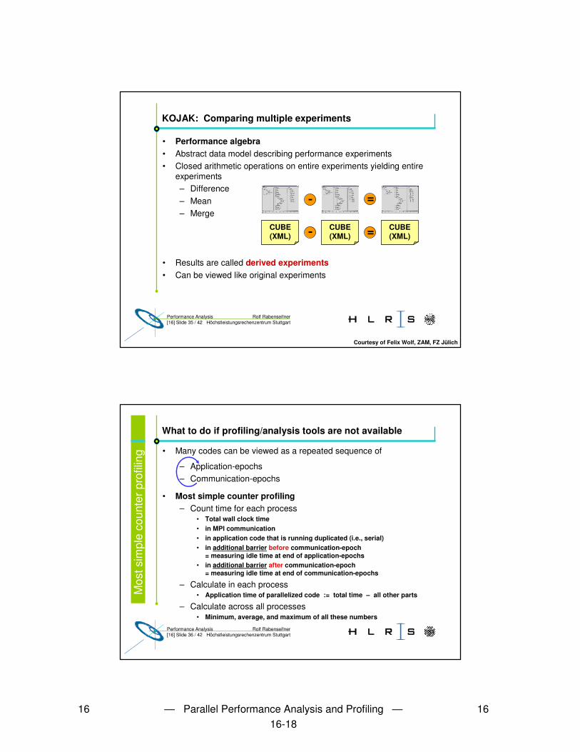
KOJAK: Comparing multiple experiments
• Performance algebra• Abstract data model describing performance experiments• Closed arithmetic operations on entire experiments yielding entire
experiments – Difference– Mean – Merge
• Results are called derived experiments• Can be viewed like original experiments
�
CUBE(XML)
CUBE(XML)
CUBE(XML)�
�
�
Courtesy of Felix Wolf, ZAM, FZ Jülich
Rolf RabenseifnerPerformance Analysis[16] Slide 36 / 42 Höchstleistungsrechenzentrum Stuttgart
What to do if profiling/analysis tools are not available
• Many codes can be viewed as a repeated sequence of
– Application-epochs– Communication-epochs
• Most simple counter profiling– Count time for each process
• Total wall clock time• in MPI communication• in application code that is running duplicated (i.e., serial)• in additional barrier before communication-epoch
= measuring idle time at end of application-epochs• in additional barrier after communication-epoch
= measuring idle time at end of communication-epochs
– Calculate in each process• Application time of parallelized code := total time – all other parts
– Calculate across all processes• Minimum, average, and maximum of all these numbers
Mos
t sim
ple
coun
ter p
rofil
ing
16 — Parallel Performance Analysis and Profiling — 1616-19
Rolf RabenseifnerPerformance Analysis[16] Slide 37 / 42 Höchstleistungsrechenzentrum Stuttgart
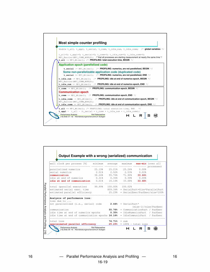
Most simple counter profiling
double t_all, t_appl, t_serial, t_comm, t_idle_num, t_idle_comm; /* global variables */
t_all=0; t_appl=0; t_serial=0; t_comm=0; t_idle_num=0; t_idle_comm=0;
MPI_Barrier(MPI_COMM_WORLD); /* that all processes are starting measurement at nearly the same time */t_all -= MPI_Wtime(); /* PROFILING: total execution time, BEGIN */
Application epoch (parellelized code)t_serial -= MPI_Wtime(); /* PROFILING: numerics, are not parallelized, BEGIN */
Some non-parallelizable application code (duplicated code)t_serial += MPI_Wtime(); /* PROFILING: numerics, are not parallelized, END */
t_idle_num -= MPI_Wtime(); /* PROFILING: idle at end of numerics epoch, BEGIN */MPI_Barrier(MPI_COMM_WORLD);
t_idle_num += MPI_Wtime(); /* PROFILING: idle at end of numerics epoch, END */
t_comm -= MPI_Wtime(); /* PROFILING: communication epoch, BEGIN */
Communication epocht_comm += MPI_Wtime(); /* PROFILING: communication epoch, END */
t_idle_comm -= MPI_Wtime(); /* PROFILING: idle at end of communication epoch, BEGIN */MPI_Barrier(MPI_COMM_WORLD);
t_idle_comm += MPI_Wtime(); /* PROFILING: idle at end of communication epoch, END */
t_all += MPI_Wtime(); /* PROFILING: total execution time, END */
t_appl = t_all - (t_serial + t_comm + t_idle_num + t_idle_comm);
Rolf RabenseifnerPerformance Analysis[16] Slide 38 / 42 Höchstleistungsrechenzentrum Stuttgart
Output Example with a wrong (serialized) communication
wall clock per process [%] minimum average maximum max-min (over all---------------------------- -------- --------- --------- --------- processes)parallelized numerics 25.19% 25.21% 25.26% 0.08%serial numerics 2.51% 2.52% 2.53% 0.02%communication 38.24% 55.76% 71.90% 33.66%idle at end of numerics 0.31% 0.35% 0.39% 0.08%idle at end of communication 0.01% 16.16% 33.68% 33.68%---------------------------- -------- --------- --------- --------- ----------total (parallel execution) 99.99% 100.00% 100.02%estimated serial exec. time 809.34% = SerialPart+Size*ParallelPartestimated parallel efficiency 25.29% = SerialExec/ParExec/size*100%--------------------------------------------------------------------------------Analysis of performance loss:loss due to ...not parallelized (i.e., serial) code 2.44% = SerialPart*
(size-1)/size/ParExeccommunication 55.76% = CommunicationPart / ParExecidle time at end of numerics epochs 0.35% = IdleNumericsPart / ParExecidle time at end of communication epochs 16.16% = IdleCommunicPart / ParExec--------------------------------------------------------------------------------total loss 74.71% = sumapproximated parallel efficiency 25.29% = 100% - total loss
Parallel P
erformance A
nalysis and Profiling [16]
16 — Parallel Performance Analysis and Profiling — 1616-20
Rolf RabenseifnerPerformance Analysis[16] Slide 39 / 42 Höchstleistungsrechenzentrum Stuttgart
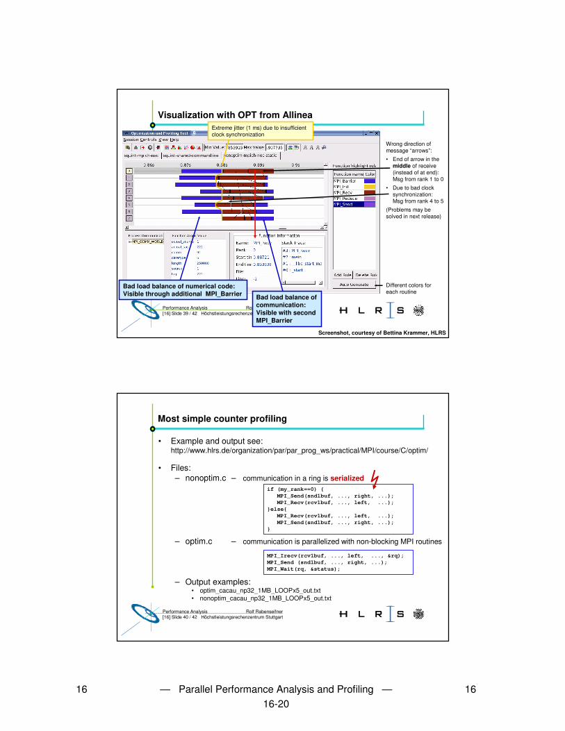
Visualization with OPT from Allinea
Different colors for each routine
Extreme jitter (1 ms) due to insufficient clock synchronization
Bad load balance of numerical code:Visible through additional MPI_Barrier Bad load balance of
communication:Visible with second MPI_Barrier
Screenshot, courtesy of Bettina Krammer, HLRS
Wrong direction ofmessage “arrows”:
• End of arrow in the middle of receive (instead of at end):Msg from rank 1 to 0
• Due to bad clock synchronization:Msg from rank 4 to 5
(Problems may besolved in next release)
Rolf RabenseifnerPerformance Analysis[16] Slide 40 / 42 Höchstleistungsrechenzentrum Stuttgart
Most simple counter profiling
• Example and output see:http://www.hlrs.de/organization/par/par_prog_ws/practical/MPI/course/C/optim/
• Files:– nonoptim.c – communication in a ring is serialized
– optim.c – communication is parallelized with non-blocking MPI routines
– Output examples:• optim_cacau_np32_1MB_LOOPx5_out.txt• nonoptim_cacau_np32_1MB_LOOPx5_out.txt
if (my_rank==0) {MPI_Send(snd1buf, ..., right, ...);MPI_Recv(rcv1buf, ..., left, ...);
}else{ MPI_Recv(rcv1buf, ..., left, ...);MPI_Send(snd1buf, ..., right, ...);
}
MPI_Irecv(rcv1buf, ..., left, ..., &rq);MPI_Send (snd1buf, ..., right, ...);MPI_Wait(rq, &status);
16 — Parallel Performance Analysis and Profiling — 1616-21
Rolf RabenseifnerPerformance Analysis[16] Slide 41 / 42 Höchstleistungsrechenzentrum Stuttgart
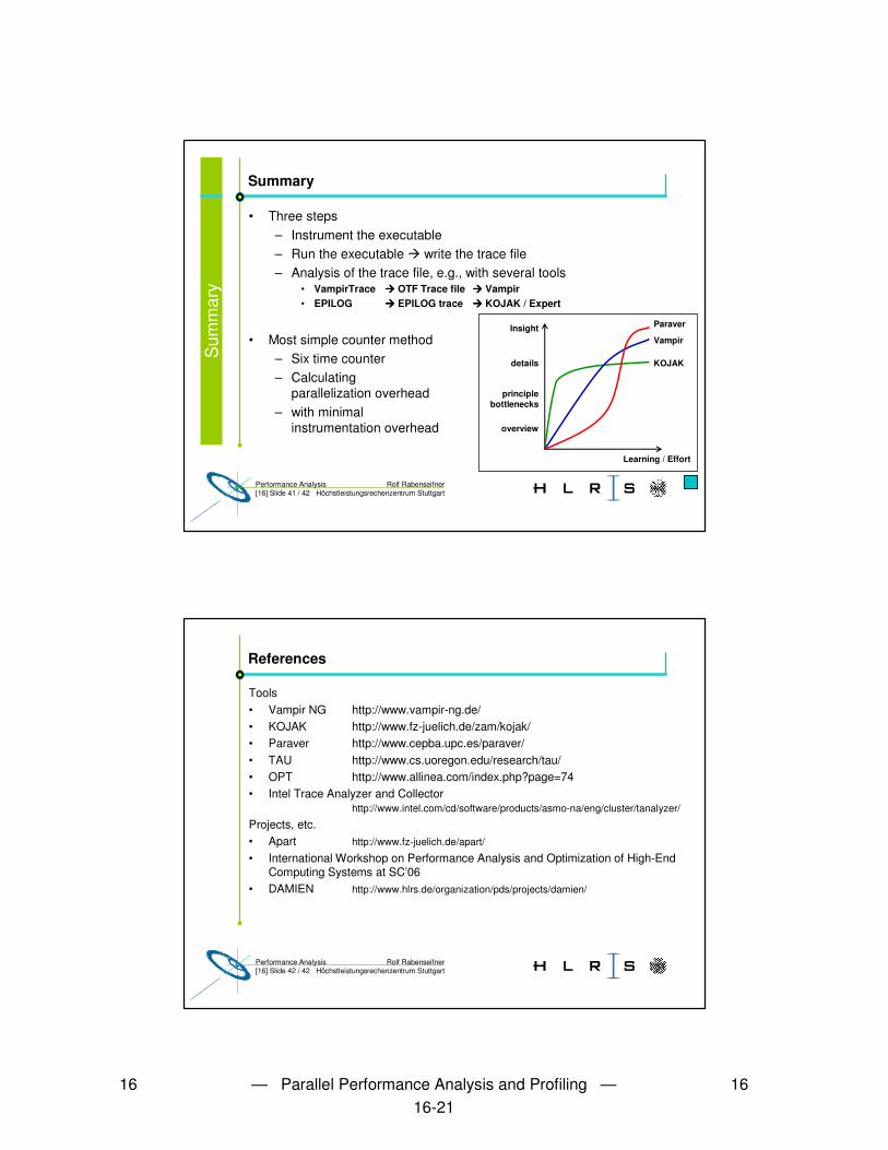
Summary
• Three steps– Instrument the executable– Run the executable � write the trace file– Analysis of the trace file, e.g., with several tools
• VampirTrace ���� OTF Trace file ���� Vampir• EPILOG ���� EPILOG trace ���� KOJAK / Expert
• Most simple counter method– Six time counter– Calculating
parallelization overhead – with minimal
instrumentation overhead
Learning / Effort
Insight
details
principlebottlenecks
overview
KOJAK
Vampir
Paraver
Sum
mar
y
Rolf RabenseifnerPerformance Analysis[16] Slide 42 / 42 Höchstleistungsrechenzentrum Stuttgart
References
Tools• Vampir NG http://www.vampir-ng.de/• KOJAK http://www.fz-juelich.de/zam/kojak/• Paraver http://www.cepba.upc.es/paraver/ • TAU http://www.cs.uoregon.edu/research/tau/• OPT http://www.allinea.com/index.php?page=74• Intel Trace Analyzer and Collector
http://www.intel.com/cd/software/products/asmo-na/eng/cluster/tanalyzer/
Projects, etc.• Apart http://www.fz-juelich.de/apart/
• International Workshop on Performance Analysis and Optimization of High-End Computing Systems at SC’06
• DAMIEN http://www.hlrs.de/organization/pds/projects/damien/


