
Karteikarten, Lineare Algebra 2,Satze und Definitionen nach der Vorlesung von
Prof. Cieliebak
Felix Muller, [email protected]
Diese Karteikartchen sollten alle Definitionen und Satze der Vorlesung ”Lineare Algebra 2” bei Herrn Cieliebak
enthalten.
Falls ihr Fehler finden solltet, dann ware es nett, wenn ihr mit ein kurzes Mail mit dem Fehler schickt.
Viel Spaß beim Lernen!
1
NICHT VERGESSEN: DUPLEX-DRUCKMODUS
+
SEITEANPASSUNG UNTER
”DATEI - DRUCKEN” -”KEINE” WAHLEN!!
Definition
Skalarprodukt
Lineare Algebra 2
Corollar 1.1
Eigenschaften des Skalarprodukts
Lineare Algebra 2
Definition
Orthogonalsystem
Lineare Algebra 2
Satz 1.1
Gram-Schmidt-Orthogonalisierung
Lineare Algebra 2
Definition
orthogonale Abbildung
Lineare Algebra 2
Corollar 1.3
U⊥ =
Lineare Algebra 2
Definition
Projektor Pu(v)
Lineare Algebra 2
Corollar 1.4
Bessel’sche Ungleichung
Lineare Algebra 2
Definition
Hermitesches Produkt
Lineare Algebra 2
Lemma 1.5
Die Abbildung V → V ∗ ist ein . . .
Lineare Algebra 2
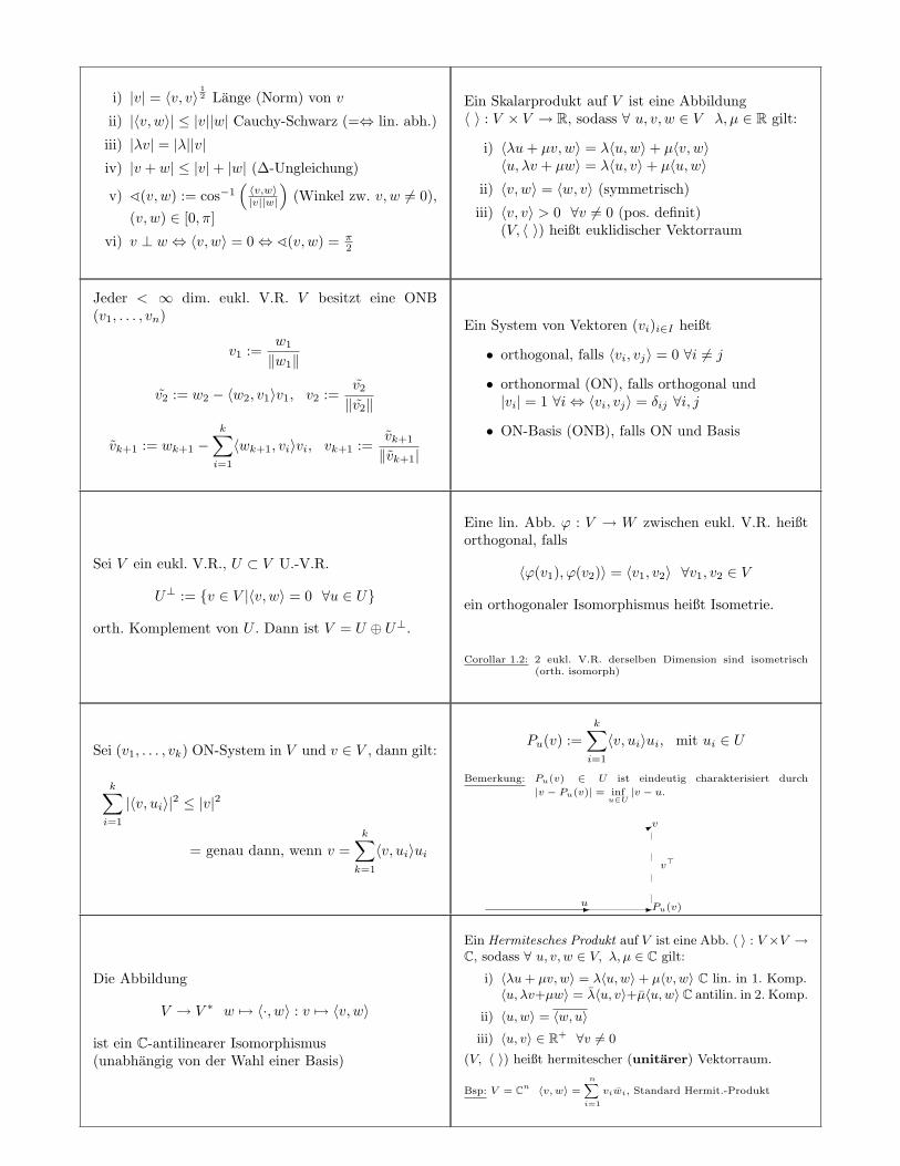
i) |v| = 〈v, v〉12 Lange (Norm) von v
ii) |〈v, w〉| ≤ |v||w| Cauchy-Schwarz (=⇔ lin. abh.)
iii) |λv| = |λ||v|iv) |v + w| ≤ |v|+ |w| (∆-Ungleichung)
v) ^(v, w) := cos−1(〈v,w〉|v||w|
)(Winkel zw. v, w 6= 0),
(v, w) ∈ [0, π]
vi) v ⊥ w ⇔ 〈v, w〉 = 0⇔ ^(v, w) = π2
Ein Skalarprodukt auf V ist eine Abbildung〈 〉 : V × V → R, sodass ∀ u, v, w ∈ V λ, µ ∈ R gilt:
i) 〈λu+ µv,w〉 = λ〈u,w〉+ µ〈v, w〉〈u, λv + µw〉 = λ〈u, v〉+ µ〈u,w〉
ii) 〈v, w〉 = 〈w, v〉 (symmetrisch)
iii) 〈v, v〉 > 0 ∀v 6= 0 (pos. definit)(V, 〈 〉) heißt euklidischer Vektorraum
Jeder < ∞ dim. eukl. V.R. V besitzt eine ONB(v1, . . . , vn)
v1 :=w1
‖w1‖
v2 := w2 − 〈w2, v1〉v1, v2 :=v2
‖v2‖
vk+1 := wk+1 −k∑i=1
〈wk+1, vi〉vi, vk+1 :=vk+1
‖vk+1|
Ein System von Vektoren (vi)i∈I heißt
• orthogonal, falls 〈vi, vj〉 = 0 ∀i 6= j
• orthonormal (ON), falls orthogonal und|vi| = 1 ∀i⇔ 〈vi, vj〉 = δij ∀i, j
• ON-Basis (ONB), falls ON und Basis
Sei V ein eukl. V.R., U ⊂ V U.-V.R.
U⊥ := {v ∈ V |〈v, w〉 = 0 ∀u ∈ U}
orth. Komplement von U . Dann ist V = U ⊕ U⊥.
Eine lin. Abb. ϕ : V → W zwischen eukl. V.R. heißtorthogonal, falls
〈ϕ(v1), ϕ(v2)〉 = 〈v1, v2〉 ∀v1, v2 ∈ V
ein orthogonaler Isomorphismus heißt Isometrie.
Corollar 1.2: 2 eukl. V.R. derselben Dimension sind isometrisch(orth. isomorph)
Sei (v1, . . . , vk) ON-System in V und v ∈ V , dann gilt:
k∑i=1
|〈v, ui〉|2 ≤ |v|2
= genau dann, wenn v =k∑k=1
〈v, ui〉ui
Pu(v) :=k∑i=1
〈v, ui〉ui, mit ui ∈ U
Bemerkung: Pu(v) ∈ U ist eindeutig charakterisiert durch
|v − Pu(v)| = infu∈U|v − u.
-u -Pu(v)
*v
v>
Die Abbildung
V → V ∗ w 7→ 〈·, w〉 : v 7→ 〈v, w〉
ist ein C-antilinearer Isomorphismus(unabhangig von der Wahl einer Basis)
Ein Hermitesches Produkt auf V ist eine Abb. 〈 〉 : V ×V →C, sodass ∀ u, v, w ∈ V, λ, µ ∈ C gilt:
i) 〈λu+ µv,w〉 = λ〈u,w〉+ µ〈v, w〉 C lin. in 1. Komp.〈u, λv+µw〉 = λ〈u, v〉+µ〈u,w〉 C antilin. in 2. Komp.
ii) 〈u,w〉 = 〈w, u〉iii) 〈u, v〉 ∈ R+ ∀v 6= 0
(V, 〈 〉) heißt hermitescher (unitarer) Vektorraum.
Bsp: V = Cn 〈v, w〉 =n∑i=1
viwi, Standard Hermit.-Produkt
Definition
Symbole Zeichen
Lineare Algebra 2
Definition
adjungierte Abbildung
Lineare Algebra 2
Definition
Eigenschaften der adjungierten Abbildung
Lineare Algebra 2
Definition
unitar,orthogonal,
unitare Gruppe,orthogonale Gruppe
Lineare Algebra 2
Satz 1.6
Spektralsatz fur selbstadjungierteEndomorphismen (C)
Lineare Algebra 2
Definition
ϕ ∈ End(V ) heißt normal ⇔
Lineare Algebra 2
Satz 1.7
Spektralsatz fur normale Endomorphismenuber C
Lineare Algebra 2
Satz 1.8
simultane Diagonalisierung furEndomorphismen
(nicht in Matrixdarstellung)
Lineare Algebra 2
Satz 1.9
Spektralsatz fur normale Endomorphismenuber R
Lineare Algebra 2
Definition
normale Matrix uber Chermitesch Matrix
Lineare Algebra 2
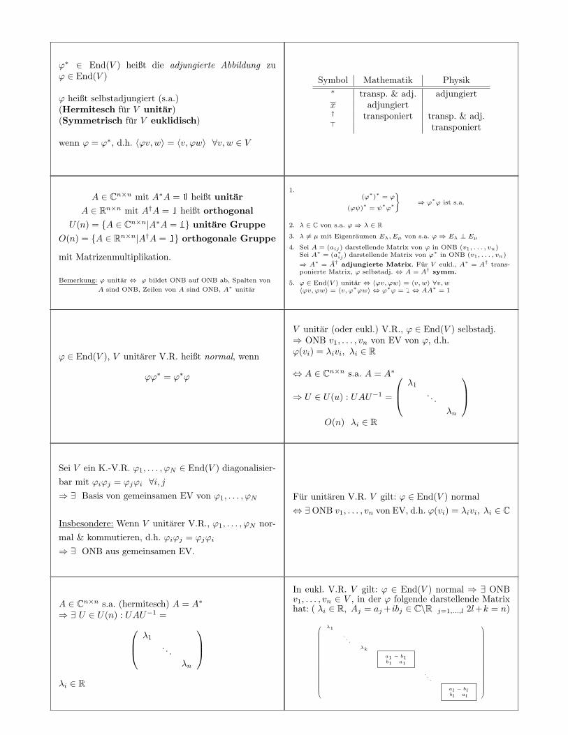
ϕ∗ ∈ End(V ) heißt die adjungierte Abbildung zuϕ ∈ End(V )
ϕ heißt selbstadjungiert (s.a.)(Hermitesch fur V unitar)(Symmetrisch fur V euklidisch)
wenn ϕ = ϕ∗, d.h. 〈ϕv,w〉 = 〈v, ϕw〉 ∀v, w ∈ V
Symbol Mathematik Physik∗ transp. & adj. adjungiertx adjungiert† transponiert transp. & adj.> transponiert
A ∈ Cn×n mit A∗A = 1 heißt unitar
A ∈ Rn×n mit A†A = 1 heißt orthogonal
U(n) = {A ∈ Cn×n|A∗A = 1} unitare Gruppe
O(n) = {A ∈ Rn×n|A†A = 1} orthogonale Gruppe
mit Matrizenmultiplikation.
Bemerkung: ϕ unitar ⇔ ϕ bildet ONB auf ONB ab, Spalten von
A sind ONB, Zeilen von A sind ONB, A∗ unitar
1.(ϕ∗)∗
= ϕ
(ϕψ)∗
= ψ∗ϕ∗
}⇒ ϕ
∗ϕ ist s.a.
2. λ ∈ C von s.a. ϕ⇒ λ ∈ R3. λ 6= µ mit Eigenraumen Eλ, Eµ von s.a. ϕ⇒ Eλ ⊥ Eµ4. Sei A = (aij) darstellende Matrix von ϕ in ONB (v1, . . . , vn)
Sei A∗ = (a∗ij) darstellende Matrix von ϕ∗ in ONB (v1, . . . , vn)
⇒ A∗ = A† adjungierte Matrix. Fur V eukl., A∗ = A† trans-ponierte Matrix, ϕ selbstadj. ⇔ A = A† symm.
5. ϕ ∈ End(V ) unitar ⇔ 〈ϕv, ϕw〉 = 〈v, w〉 ∀v, w〈ϕv, ϕw〉 = 〈v, ϕ∗ϕw〉 ⇔ ϕ∗ϕ = 1⇔ AA∗ = 1
ϕ ∈ End(V ), V unitarer V.R. heißt normal, wenn
ϕϕ∗ = ϕ∗ϕ
V unitar (oder eukl.) V.R., ϕ ∈ End(V ) selbstadj.⇒ ONB v1, . . . , vn von EV von ϕ, d.h.ϕ(vi) = λivi, λi ∈ R
⇔ A ∈ Cn×n s.a. A = A∗
⇒ U ∈ U(u) : UAU−1 =
λ1
. . .λn
O(n) λi ∈ R
Sei V ein K.-V.R. ϕ1, . . . , ϕN ∈ End(V ) diagonalisier-bar mit ϕiϕj = ϕjϕi ∀i, j⇒ ∃ Basis von gemeinsamen EV von ϕ1, . . . , ϕN
Insbesondere: Wenn V unitarer V.R., ϕ1, . . . , ϕN nor-mal & kommutieren, d.h. ϕiϕj = ϕjϕi
⇒ ∃ ONB aus gemeinsamen EV.
Fur unitaren V.R. V gilt: ϕ ∈ End(V ) normal⇔ ∃ ONB v1, . . . , vn von EV, d.h. ϕ(vi) = λivi, λi ∈ C
A ∈ Cn×n s.a. (hermitesch) A = A∗
⇒ ∃ U ∈ U(n) : UAU−1 = λ1
. . .λn
λi ∈ R
In eukl. V.R. V gilt: ϕ ∈ End(V ) normal ⇒ ∃ ONBv1, . . . , vn ∈ V , in der ϕ folgende darstellende Matrixhat: ( λi ∈ R, Aj = aj+ ibj ∈ C\R j=1,...,l 2l+k = n)
λ1
. . .λk
a1 − b1b1 a1
. . .
al − blbl al
Definition
normale Matrix uber Cschief-hermitesch Matrix
Lineare Algebra 2
Definition
normale Matrix uber Cunitar Matrix
Lineare Algebra 2
Satz 1.8.2
simultane Diagonalisierung fur Matrizen
Lineare Algebra 2
Definition
normale Matrix uber Rsymmetrische Matrix
Lineare Algebra 2
Definition
normale Matrix uber Rschief-symmetrische Matrix
Lineare Algebra 2
Definition
normale Matrix uber Rorthogonale Matrix
Lineare Algebra 2
Definition
Spezielle unitare Gruppespezielle orthogonale Gruppe
Lineare Algebra 2
Definition
Bilinearform
Lineare Algebra 2
Definition
Eigenschaften von Bilinearformen
Lineare Algebra 2
Definition
Nullraum von γ
Lineare Algebra 2
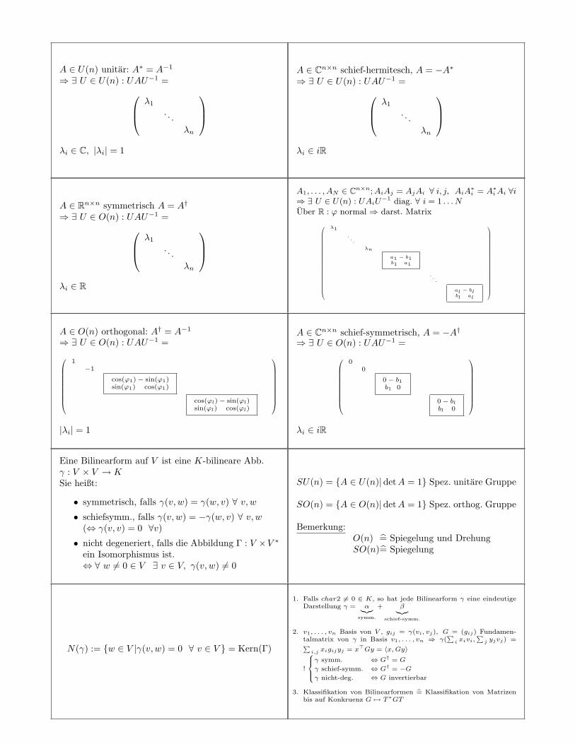
A ∈ U(n) unitar: A∗ = A−1
⇒ ∃ U ∈ U(n) : UAU−1 = λ1
. . .λn
λi ∈ C, |λi| = 1
A ∈ Cn×n schief-hermitesch, A = −A∗⇒ ∃ U ∈ U(n) : UAU−1 = λ1
. . .λn
λi ∈ iR
A ∈ Rn×n symmetrisch A = A†
⇒ ∃ U ∈ O(n) : UAU−1 = λ1
. . .λn
λi ∈ R
A1, . . . , AN ∈ Cn×n;AiAj = AjAi ∀ i, j, AiA∗i = A∗iAi ∀i
⇒ ∃ U ∈ U(n) : UAiU−1 diag. ∀ i = 1 . . . N
Uber R : ϕ normal ⇒ darst. Matrix
λ1
. . .λn
a1 − b1b1 a1
. . .
al − blbl al
A ∈ O(n) orthogonal: A† = A−1
⇒ ∃ U ∈ O(n) : UAU−1 =
1−1
cos(ϕ1)− sin(ϕ1)sin(ϕ1) cos(ϕ1)
cos(ϕl)− sin(ϕl)sin(ϕl) cos(ϕl)
|λi| = 1
A ∈ Cn×n schief-symmetrisch, A = −A†⇒ ∃ U ∈ O(n) : UAU−1 =
00
0− b1b1 0
0− blbl 0
λi ∈ iR
Eine Bilinearform auf V ist eine K-bilineare Abb.γ : V × V → KSie heißt:
• symmetrisch, falls γ(v, w) = γ(w, v) ∀ v, w• schiefsymm., falls γ(v, w) = −γ(w, v) ∀ v, w
(⇔ γ(v, v) = 0 ∀v)
• nicht degeneriert, falls die Abbildung Γ : V ×V ∗ein Isomorphismus ist.⇔ ∀ w 6= 0 ∈ V ∃ v ∈ V, γ(v, w) 6= 0
SU(n) = {A ∈ U(n)|detA = 1} Spez. unitare Gruppe
SO(n) = {A ∈ O(n)|detA = 1} Spez. orthog. Gruppe
Bemerkung:O(n) = Spiegelung und DrehungSO(n)= Spiegelung
N(γ) := {w ∈ V |γ(v, w) = 0 ∀ v ∈ V } = Kern(Γ)
1. Falls char2 6= 0 ∈ K, so hat jede Bilinearform γ eine eindeutigeDarstellung γ = α︸︷︷︸
symm.
+ β︸︷︷︸schief-symm.
2. v1, . . . , vn Basis von V , gij = γ(vi, vj), G = (gij) Fundamen-talmatrix von γ in Basis v1, . . . , vn ⇒ γ(
∑i xivi,
∑j yjvj) =∑
i,j xigijyj = x>Gy = 〈x,Gy〉
!
γ symm. ⇔ G† = G
γ schief-symm. ⇔ G† = −Gγ nicht-deg. ⇔ G invertierbar
3. Klassifikation von Bilinearformen = Klassifikation von Matrizenbis auf Konkruenz G 7→ T∗GT
Definition
isotrop, koisotrop
Lineare Algebra 2
Satz 1.10
Hauptachsentransformation(Diagonalisierung symm. Bilinearformen)
Lineare Algebra 2
Corollar 1.11
Sei G symm. in K. Falls ∀ λ ∈ K einQuadrat ist ⇒ ∃ T ∈ GL(n,K)
Lineare Algebra 2
Definition
Rang & Index einer Matrix
Lineare Algebra 2
Satz 1.12
Tragheitssatz von Sylvester
Lineare Algebra 2
Definition
Quadratische Form
Lineare Algebra 2
Corollar 1.13
Corollar aus simultaner Diagonalisierung
Lineare Algebra 2
Satz 1.14
schiefsymm. Bilinearformen, Darstellung derFundamentalmatrix
Lineare Algebra 2
Definition
Zerlegungen von Matrizen
Lineare Algebra 2
Lemma 2.1
B = D ·N - Zerlegung
Lineare Algebra 2
Sei γ symm. Bilinearf. auf K.-V.R. V char2 6= 0 in K.⇒ ∃ ONB v1, . . . , vn fur γ, d.h.
γ(vi, vj) = λiδij , λi ∈ K
In Fundamentalmatrix G ausgedruckt.∀ G ∈ Kn×n symm. ∃ T ∈ GL(n,K) sodass T †GT = λ1
. . .λn
U> := {v ∈ V |γ(u, v) = 0 ∀u ∈ U}
U heißt:
• isotrop, falls U ⊂ U>
• koisotrop, falls U> ⊂ U
Fur eine symm. Bilinearform γ mit Fund.-Matrix G:
Rang(γ) := dimV − dimN(γ) = Rang(G)
K = R : Index(γ) := max{dimU |U ⊂ V U.-V.R. mitγ|U neg. definit, d.h. γ(u, u) < 0 ∀ 0 6= u ∈ U}
Bemerkung:Rang(G) = Anzahl der ±1 in Corollar 1.11Index(G) = Anzahl der −1 in Corollar 1.11
Sei G inKn×n symm. char2 6= 0 in K.
a) Falls jedes λ ∈ K ein Quadrat ist (z.B. K = C),so ∃ T ∈ GL(n,C)
T†GT =
0
. . .1
. . .
b) Fur K = R ∃ T ∈ GL(n,R)
T†GT =
0
. . .1
. . .−1
. . .
γ : V × V → K symm. Bilinearform, dann heißt dieAbb. γ : V → K, v 7→ γ(v, v) die quadratische Formvon γ.
Zwei symm. Matrizen in Kn×n sind genau dann kon-kruent, wenn sie{
denselben Rang (K = C) habendenselben Rang und Index (K = R) haben
Sei ω eine nicht-deg. schief-symm. Bilinearform auf V .⇒ ∃ Basis e1, f1, e2, f2, . . . von V mit{
ω(ei, ej) = ω(fi, fj) = 0 ∀ i, jω(ei, fj) = δij
d.h. die Fundamentalmatrix von ω in Basise1, f1, . . . , em, fm ist:
e1f1...
.
.
.emfm
0 1−1 0
0 1−1 0
. . .
0 1−1 0
Bemerkung: Insbesondere ist dimV = 2m gerade.
Seien G1, G2 ∈ Rn×n symmetrisch, G1 pos. definit⇒ ∃ T ∈ GL(n,R) mit
T †G1T = 1
T †G2T =
(λ1
. . .λn
), λi ∈ R
Jedes B ∈ B±(n,K) hat eine eindeutige ZerlegungB = D ·N mit D ∈ D(n,K), N ∈ N±(n,K).
Beweis:
Existenz: D := Diagonale von B.
N := D−1 · B ∈ N±(n,K)
Eindeutigkeit: B = D1N1 = D2N2
⇒ D−11 D2 = N1N
−12 ∈ D(n,K) ∩N±(n,K) = {1}
⇒ D1 = D2, N1 = N2
D(n,K) := {A ∈ GL(n,K)|aij = 0 ∀ i, j}(Diagonalmatrixen)
∩GL(n,K) ⊃ B±(n,K) := {A ∈ GL|aij = 0 ∀ i ≷ j}
(obere, untere ∆-Matrizen)
∪N±(n,K) := {A ∈ B±(n,K)|aii = 1 ∀ i}( 1 ∗ ∗
0 · ∗0 0 1
)
Satz 2.2
PLR-Zerlegung
Lineare Algebra 2
Definition
LR-Zerlegung
Lineare Algebra 2
Definition
QR-Zerlegung
Lineare Algebra 2
Corollar 2.4
Iwasawa-Zerlegung
Lineare Algebra 2
Definition
Hermitesche Matrix H
Lineare Algebra 2
Corollar 2.5
Jede hermitesche Matrix hat eine eindeutigeZerlegung
Lineare Algebra 2
Satz 2.6
Quadratwurzel
Lineare Algebra 2
Corollar 2.7
Polarzerlegung
Lineare Algebra 2
Satz 2.8
multiplikative Jordan-Chevalley-Zerlegung
Lineare Algebra 2
Definition
Frobenius Norm
Lineare Algebra 2

A = (. . .) Gauß−−−−−−→
Schreibw.
(A∣∣∣ 1
11
)Gauß−−−→
( ∗ ∗ ∗∗ ∗∗︸ ︷︷ ︸
=R
∣∣∣ · · 0· · ·· · ·︸︷︷︸
=L−1
)
Bsp:A = ( 3 2
6 6 ) ⇒ ( 3 26 6 | 1 0
0 1 ) ⇔(
3 20 2
∣∣ 1 0−2 1
)⇔(
1 0−2 1 | 1 0
0 1
)⇔ ( 1 0
0 1 | 1 02 1 )
⇒ Ax = b⇔ LRx = b⇔ Rx = L−1b
Jede invertierbare Matrix hat eine (i.A. nicht eindeu-tige) Zerlegung:
A = PLR , mit
P ∈ P (n) Permutations-MatrixL ∈ N−(n,K) linke, untere ∆-Matrix mit aii = 1R ∈ B+(n,K) rechte, obere ∆-Matrix
Jedes A ∈ GL(n,C) hat eine eindeutige ZerlegungA = QDN
Q ∈ U(n) unitare MatrixD ∈ D(n) aii 6= 0, sonst 0N ∈ N+(n,C) rechte, obere ∆-Matrix mit aii = 1
Jedes A ∈ GL(n,C/R) hat eine eindeutige Zerlegung
A = QR , Q ∈ U(n)/O(n), R ∈ ∆+(n,C/R)
A = (. . .)
Gram-Schmidt−−−−−−−−−→auf Spalten
u1 =
(...
), . . . , un =
(...
)(u1 . . . un) = Q⇒ Q−1 = Q† ⇒ A = QR⇒ Q†A = R
Bsp: A =( 2 3
1 0
)→ u1 = 1√
5
( 21
)u2 = v2 − 〈v2, u1〉u1 ⇒ u2 =
u2‖u2‖
=(
0,61,2
)⇒ Q =
(2√5
0,6
1√5
1,2
)⇒ Q−1 =
(2√
53 −
√5
3− 5
9109
)⇒ Q−1A = R
⇒ Q−1A =
(√5 2√
50 − 5
3
)= R
Jedes H ∈ H+(n,C) hat eine eindeutige ZerlegungH = N∗DN
D ∈ D(n) aii 6= 0, sonst 0N ∈ N+(n,C) rechte, obere ∆-Matrix mit aii = 1
(spezielle Hauptachsentransformation)
H+(n,C) := {H ∈ Cn×n|H = H∗, H > 0}
H > 0 : H pos. definit, d.h. x>Hx > 0 ∀ x 6= 0 ∈ C
Jedes A ∈ GL(n,R/C) hat eine eindeutige ZerlegungA = HQ, H ∈ H+(n,R/C), Q ∈ U(n)/O(n)
A = Q√A∗A =
√A∗AQ⇒ Q = A(
√A∗A︸ ︷︷ ︸
zu diag.
)−1 = (√A∗A)−1A
1. Berechne A∗A
2. Berechne EW und U bzw. U−1 ⇒(EW1
·EWn
)3. H = U−1√DU mit U−1 = (EV1 . . . EVn)
4. Q = H−1A
Zu jedem H ∈ H+(n,C) ∃√H ∈ H+(n,C) mit√
H2
= H.
Fur A,B ∈ Cn×n sei 〈A,B〉 = tr(AB†) =∑ni,j=1 aijbij ∈ C
Standard Hermitesches Produkt auf Cn×n ∼= C(K2)
‖A‖ := 〈A,A〉12 =
∑ni,j=1 |aij |2 Norm auf A.
es gilt:
i) ‖A‖ ≥ 0, = 0⇔ A = 0
ii) ‖λA‖ = |λ|‖A‖, λ ∈ Ciii) ‖A+ B‖ ≤ ‖A‖+ ‖B‖
iv) ‖A · B‖ ≤ ‖A‖ · ‖B‖
v) ‖TAT−1‖ = ‖A‖ · ‖T‖ · ‖T−1‖
Jedes A ∈ GL(n,C) hat eine eindeutige Zerlegung.A = Γ(1+N) ΓN = NΓ, Γ halbeinfach, N nilpotent.
1. Bestimme EW λ1, . . . , λn paarweise verschieden (A ∈ Cn×n)
χA(x) = (x− λ1)m1 . . . (x− λk)mk
2. Bestimme Basen (vim1. . . vimi
) von
Hau(Aiλi) = Kern(A− λi1)mi → wahle Basis beliebig
T := (v11 . . . v
1m1
. . . vk1 . . . vkmk
) Basis von Cn
3. Γ :=
(λ1
λ1·λk
)⇒ T−1AT − Γ =: N ist nilpotent
[Γ, N ] = 0, Γ := T ΓT−1, N = TNT−1 = A− Γ, A = Γ +N
[Γ, N ] = 0, Γ diag., N nilpotent.
Lemma 2.9
Konvergenz einer Potenzreihe
Lineare Algebra 2
Definition
Exponential- & Logarithmusreihe
Lineare Algebra 2
Definition
Spec(Γ) := . . .
Lineare Algebra 2
Definition
Eigenschaften der Exp-Funktion
Lineare Algebra 2
Satz 2.10
exp : Φn×n → GL(n,C) ist surjektiv.
Lineare Algebra 2
Lemma 2.11
Sei f(z) =∑fkz
k Konv.-Radius Rf , f(0) = 0g(z) =
∑gkz
k Konv.-Radius Rg, g(0) = 0
Sei R := sup{r < Rf |∑|fk|rk < Rg} > 0 und
g(f(z)) = z ∀ z ∈ Φ mit |z| < R
dann gilt: . . .
Lineare Algebra 2
Anwendung
Anwendung auf exp / log
Lineare Algebra 2
Satz 2.12
W&V offene Umgebungen, sodass W,Vzueinander inverse Homoomorphismen
(Diffeomorphismen) sind. W kann so gewahltwerden, dass gilt . . .
Lineare Algebra 2
Definition
Liealgebra LG von G
Lineare Algebra 2
Definition
wichtige Liegruppenu(n), o(n), su(n), so(n)
Lineare Algebra 2
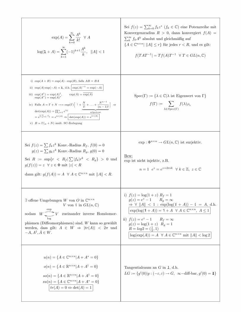
exp(A) =∞∑k=0
Ak
k!∀ A
log(1 +A) =∞∑k=1
(−1)k+1Ak
k, ‖A‖ < 1
Sei f(z) =∑∞k=0 fkz
∗ (fk ∈ C) eine Potenzreihe mitKonvergenzradius R > 0, dann konvergiert f(A) =∑∞k fkA
k absolut und gleichmaßig auf{A ∈ Cn×n| ‖A‖ ≤ r} fur jedes r < R, und es gilt:
f(TAT−1| = Tf(A)T−1 ∀ T ∈ GL(n,C)
i) exp(A+ B) = exp(A) · exp(B), falls AB = BA
ii) exp(A) exp(−A) = 1, d.h. exp(A)−1
= exp(−A)
iii) exp(A†) = exp(A)†, exp(A) = exp(A)exp(A∗) = exp(A)∗
iv) Falls A = Γ +N →= exp(Γ)[1 +
N
1!+ . . .+
Nn−1
(n− 1)!︸ ︷︷ ︸nilpotent
]⇒
det(exp(A)) =∏nj=1 e
λj
= e∑nj=1 λj = etr(A) ⇒ det(exp(A)) = e
tr(A)
v) B = Γ(1 +N) mult. SC-Zerlegung
Spec(Γ) := {λ ∈ C|λ ist Eigenwert von Γ}
f(Γ) :=∑
λ∈Spec(Γ)
f(λ)Pλ
Sei f(z) =∑fkz
k Konv.-Radius Rf , f(0) = 0g(z) =
∑gkz
k Konv.-Radius Rg, g(0) = 0
Sei R := sup{r < Rf |∑|fk|rk < Rg} > 0 und
g(f(z)) = z ∀ z ∈ Φ mit |z| < R
dann gilt: g(f(A)) = A ∀ A ∈ Cn×n mit ‖A‖ < R.
exp : Φn×n → GL(n,C) ist surjektiv.
Bew:exp ist nicht injektiv, z.B.
n = 1 ez = ez+2πik ∀ k ∈ Z, z ∈ C
∃ offene Umgebungen W von O in Cn×nV von 1 in GL(n,C)
sodass W
exp))V
log
jj zueinander inverse Homoomor-
phismen (Diffeomorphismen) sind. W kann so gewahltwerden, dass gilt: A ∈ W ⇒ |tr(A)| < 2π und−A,A†, A ∈W .
i) f(z) = log(1 + z) Rf = 1g(z) = ez − 1 Rg =∞⇒ ∀ ‖A‖ < 1 : exp(log(1 + A)) − 1 = A, d.h.
exp(log(1 +A)) = 1 +A ∀ A ∈ Cn×n, A ≤ 1
ii) f(z) = ez − 1 Rf =∞g(z) = log(1 + z) Rg = 1R = log2 = (1
2 , 1)
log(exp(A)) = A ∀ A ∈ Cn×n mit ‖A‖ < log 2
u(n) = {A ∈ Cn×n|A+A∗ = 0}
o(n) = {A ∈ Rn×n|A+A† = 0}
so(n) = {A ∈ Rn×n|A+A† = 0}su(n) = {A ∈ Cn×n|A+A∗ = 0}
tr(A) = 0⇔ det(A) = 1
Tangentialraum an G in 1, d.h.LG := {g′(0)|g : (−ε, ε)→ G, ∞−diff-bar, g′(0) = 1}
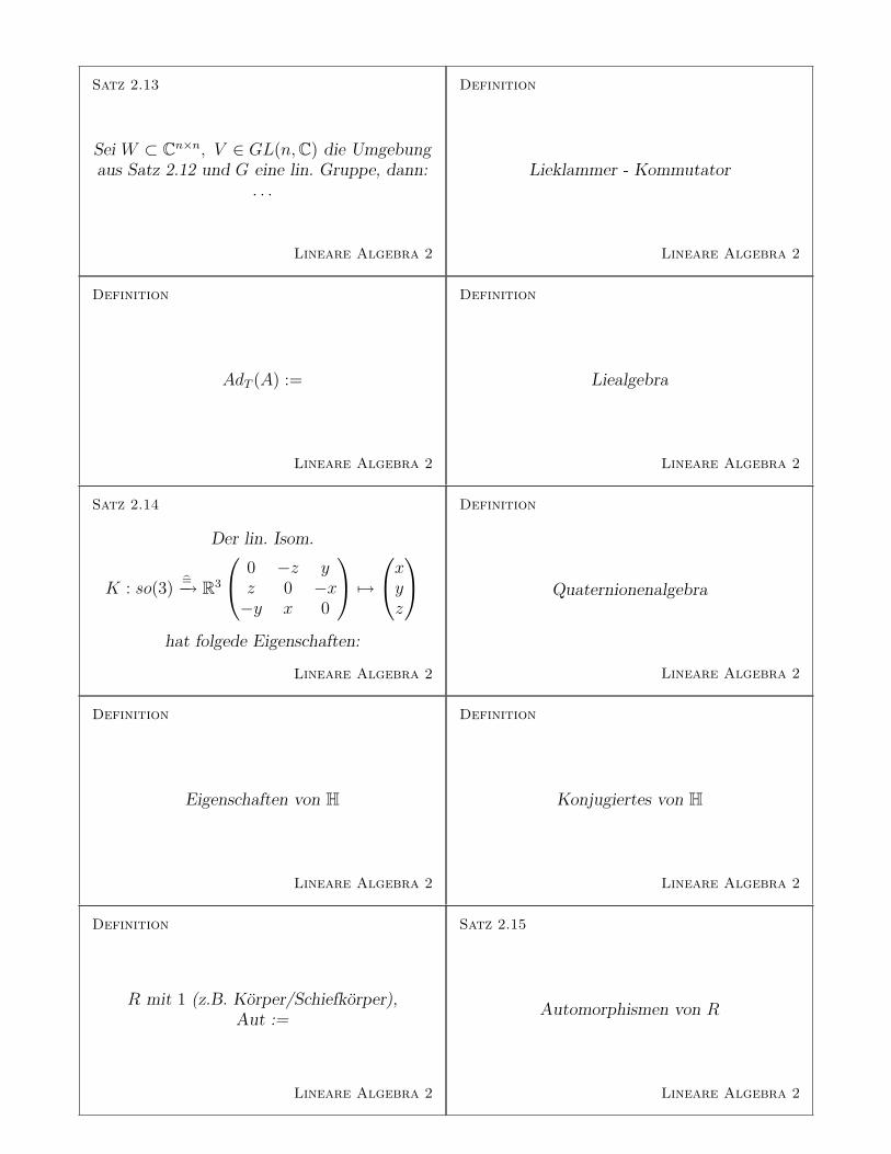
Satz 2.13
Sei W ⊂ Cn×n, V ∈ GL(n,C) die Umgebungaus Satz 2.12 und G eine lin. Gruppe, dann:
. . .
Lineare Algebra 2
Definition
Lieklammer - Kommutator
Lineare Algebra 2
Definition
AdT (A) :=
Lineare Algebra 2
Definition
Liealgebra
Lineare Algebra 2
Satz 2.14
Der lin. Isom.
K : so(3)=−→ R3
0 −z yz 0 −x−y x 0
7→xyz
hat folgede Eigenschaften:
Lineare Algebra 2
Definition
Quaternionenalgebra
Lineare Algebra 2
Definition
Eigenschaften von H
Lineare Algebra 2
Definition
Konjugiertes von H
Lineare Algebra 2
Definition
R mit 1 (z.B. Korper/Schiefkorper),Aut :=
Lineare Algebra 2
Satz 2.15
Automorphismen von R
Lineare Algebra 2

Kommutator (Lieklammer) von A,B,∈ LG :
[A,B] = AB −BA
Bemerkung: wichtige Beobachtung:
A,B ∈ LG⇒ [A,B] ∈ LG
Sei W ⊂ Cn×n, V ∈ GL(n,C) die Umgebung aus Satz2.12 und G eine lin. Gruppe, dann:
exp(W ∩ LG) = V ∩GFolgerungen:
• W ∩ LG
exp))V
log
jj ∩G sind zueinander inverse Homoom.
• A ∈ GL, ε > 0 : tA ∈ W ∀ |t| < ε mit t ∈ R⇒ g(t) := exp(tA) g : (−ε, ε)→ G ist ∞-oft diff-bar
g(0) = 1, g′(0) = A
Eine Liealgebra uber dem Korper K ist ein K-V.R. Lmit einer bilinearen Abbildung [, ] : L× L→ L
1. [X,X] = 0 ∀ x (schiefsymm.)(⇒ [X,Y ] = −[Y,X] ∀ X,Y )
2. [[X,Y ], Z]+[[Y,Z], X]+[[Z,X], Y ] = 0 ∀X,Y, Z(Jacobi-Identitat)
Eine lin. Abb. ϕ : (L, [ ]) → (L′, [ ]′) heißt Hom. vonLiealgebren, wenn [ϕ(X), ϕ(Y )]′ = ϕ([X,Y ]) ∀X,Y
d
dt
∣∣∣∣t=0
T exp(tA)T−1 = TAT−1 =: AdT (A)
d
dt
∣∣∣∣t=0
Adexp(tA)B = [A,B]
Die QuaternionenAlgebra H ist der 4− dim R-V.R. H mitBasis 1, i, j, k und der R-bilinearen Multiplikation1 · x = x · 1 = x ∀ x ∈ H,i2 = j2 = k2 = ijk = −1,ij = −ji = k, jk = −kj = i, ki = −ik = jes gilt:
• R bilinear ⇒ distributiv
• assoziativ (z.B. (ij)i = ki = j, i(ji) = i(−k) = j . . .
• ∀ x 6= 0 ∃ x−1 : xx−1 = x−1x = 1
• nicht kommutativ ij 6= ji
i) K([X,Y ]) = K(X)×K(Y ), d.h. K : (so(3), [ , ])=−→
(R3, x) ist Isomorphismus von Liealgebren
ii) K−1(v) : R3 → R3, v ∈ R3, w 7→ v × wiii) K(T × T−1) = T ·K(x) ∀ T ∈ so(3), x ∈ so(3)
iv) |K(x)|2 = 12tr(XX†), d.h. K : (so(3), 1
2tr(xy†)) →
(R3, <>) ist orthogonal
v) exp(x), 0 6= x ∈ so(3) ist eine Drehung um AchseK(x)|K(x)| mit Geschw. |K(x)|
Bemerkung: Jede Drehung im SO(3) ist Produkt von 3 Drehungenum x, y, z-Achse
x = x0 − x1i− x2j − x3k = Re(x)− Im(x)
es gilt: xy = yx, also x ⊥ y ⇔ xy = −yx
i) x = x0︸︷︷︸Re(x)
+ x1i+ x2j + x3k︸ ︷︷ ︸Im(x)
ii) R = ReH = Z(H) = {x ∈ H | xy = yx ∀ y ∈ H}
iii) |x| = 〈x, x〉12 xx = |x|2 = xx⇒ x−1 = x
|x|2
|xy|2 = xy(xy) = xyyx = |x|2|y|2 ⇒ |xy| = |x||y|
iv) x, y ∈ Im(H)→ Im(xy) = (x2y3−x3y2)i+(x3y1−x1y3)j+(x1y2 − x2y1)k ⇒ Im(xy) = x · y ∀ x, y ∈ Im(H) ∼= R3
v) (xy)2 = xyxy = −x2y2 ∈ R≤0
2〈x, y〉 = xy + yx weil: 〈X,Y 〉 = 12 (XY ∗ + Y X∗) ⇒
2〈x, y〉y = xyy + yxy⇒ yxy = α〈x, y〉y − 〈y, y〉x ∀ x, y ∈ H
Aut(H)︸ ︷︷ ︸Ringstruktur
= {ϕ ∈ SO(H)|ϕ(1) = 1} ∼= SO(Im(H))︸ ︷︷ ︸metr.Struktur,‖ ‖
R mit 1 (z.B. Korper/Schiefkorper)
Aut(R) = {ϕ : Rbij−−→ R | ϕ(1) = 1,
ϕ(x+ y) = ϕ(x) + ϕ(y), ϕ(xy) = ϕ(x) · ϕ(y)}
Definition
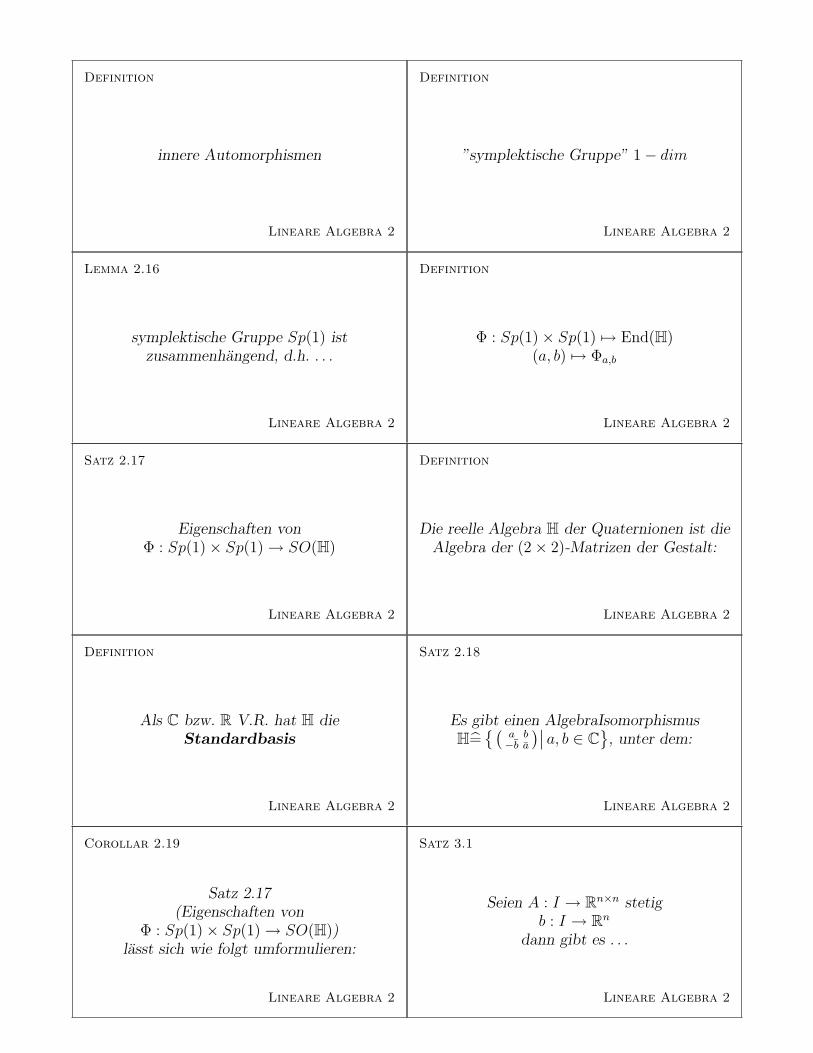
innere Automorphismen
Lineare Algebra 2
Definition
”symplektische Gruppe” 1− dim
Lineare Algebra 2
Lemma 2.16
symplektische Gruppe Sp(1) istzusammenhangend, d.h. . . .
Lineare Algebra 2
Definition
Φ : Sp(1)× Sp(1) 7→ End(H)(a, b) 7→ Φa,b
Lineare Algebra 2
Satz 2.17
Eigenschaften vonΦ : Sp(1)× Sp(1)→ SO(H)
Lineare Algebra 2
Definition
Die reelle Algebra H der Quaternionen ist dieAlgebra der (2× 2)-Matrizen der Gestalt:
Lineare Algebra 2
Definition
Als C bzw. R V.R. hat H dieStandardbasis
Lineare Algebra 2
Satz 2.18
Es gibt einen AlgebraIsomorphismusH=
{(a b−b a
)∣∣ a, b ∈ C}
, unter dem:
Lineare Algebra 2
Corollar 2.19
Satz 2.17(Eigenschaften von
Φ : Sp(1)× Sp(1)→ SO(H))lasst sich wie folgt umformulieren:
Lineare Algebra 2
Satz 3.1
Seien A : I → Rn×n stetigb : I → Rn
dann gibt es . . .
Lineare Algebra 2

Sp(1) := {a ∈ H| |a| = 1} ∼= S3 ⊂ R4 ∼= H
ist Gruppe Mult. in H ”symplektische Gruppe” 1−dim
0 6= a ∈ H→ Ada : H→ H, Ada(x) := axa−1
es gilt:
• Ada(xy) = Ada(x) ·Ada(y), d.h. Ada ∈ Aut(H)
• Adab = Ada ◦ Adb, d.h. Ad : (H\{0}, ·) →(Aut(H), ◦) ist Gruppenhom.
Inn(H) := {Ada|0 6= a ∈ H} ⊂ Aut(H) heißt Gruppeder inneren Automorphismen.
Φ : Sp(1)× Sp(1) 7→ End(H)
(a, b) 7→ Φa,b
Φa,b(x) := a× b = a× b−1
|Φa,b(x)| = |a| × |b|(= 1× 1) = |x|
symplektische Gruppe Sp(1) ist zusammenhangend,d.h. ∀ a ∈ Sp(1) ∃ stetiger Weg γ : [0, 1] → Sp(1)mit j(0) = 1 j(1) = a
Die reelle Algebra H der Quaternionen ist die Algebrader (2× 2)-Matrizen der Gestalt:
H={(
a b−b a
)∣∣∣∣ a, b ∈ C}
=
{(x0 + ix1 x2 + ix3
−x2 + ix3 x0 − ix1
)∣∣∣∣xi ∈ R, i=0,1,2,3
}a) Φ : Sp(1) × Sp(1) → SO(H) ist surjektiv mit
Kern Φ = {(1, 1), (−1,−1)}b) Ad : Sp(1) → Aut(H) ∼= SO(ImH) ist surjektiv
mit KernAd = {1,−1}
• 1 = ( 1 00 1 ) & i =
(i 00 −i
)& j =
(0 1−1 0
)&
k = ( 0 ii 0 )
• Sp(1) ∼= SU(2)
• Im(H) ∼= su(2)
• Konjugation in H = X 7→ X∗
C : 1 =(
1 00 1
)& j =
(0 1−1 0
)
R : 1 =(
1 00 1
)& i =
(i 00 −i
)&
j =(
0 1−1 0
)& k =
(0 ii 0
)
Seien A : I → Rn×n stetigb : I → Rn
dann gibt es zu t0 ∈ I und x0 ∈ Rn genau eine Losungx : I → Rn von (2) mit Anfangsbedingung x(t0) = x0
(1) heißt lineare Differentialgleichung
x′ = A(t)x (1)
x′ = A(t)x+ b(t) (2)
a) Φ, SU(2)× SU(2)→ SO(H) ∼= SO(4)(A,B) 7→ [X 7→ A×B∗] ist surjektiv mitKern Φ = {(1,1), (−1,−1)}
b) Ad : SU(2)→ SO(ImH) ∼= SO(3) ∼= SO(su(2))A 7→ [X 7→ A × A−1] ist surjektiv mitKernAd{1,−1}

Lemma 3.2
Was sind die Losungen von
x′ = A(t)x (1)
und die Anfangswertabb.(t0 ∈ I)
Lineare Algebra 2
Lemma 3.3
Was sind die Losungen von
x′ = A(t)x+ b(t) (2)
Lineare Algebra 2
Definition
Fundamentalmatrix
Lineare Algebra 2
Satz 3.4
Variation der Konstanten
Lineare Algebra 2
Lemma 3.5
Die normalisierteLosungs-Fundamental-Matrix von x′ = Ax
ist:
Lineare Algebra 2
wichtiger Spezialfall (DGL)
x′ = Ax→ ψ(t) = exp(tA)A diag-bar mit EV Avi = λivi, i=1...n
Lineare Algebra 2
Corollar 3.6.1
Zu b0 ∈ I und x0, . . . , xn−1 ∈ C ∃ ! Lsgx : I → C von
x(n)+an−1(t)x(n−1)+. . .+a1(t)x′+a0(t)x = b(t)
mit Anfangsbed:
Lineare Algebra 2
Corollar 3.6.2
Lhom = {Lsg x : I → C von
x(n)+an−1(t)x(n−1)+. . .+a1(t)x′+a0(t)x = 0}
ist U-V.R. von Cn(I,Cn) und dieAnfangswertabb. (fur T0 ∈ I)
Lineare Algebra 2
Corollar 3.6.3
Wronskideterminante
Lineare Algebra 2
Corollar 3.6.4
Losung von inhom. DGL
Lineare Algebra 2
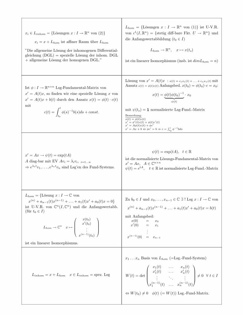
xi ∈ Linhom = {Losungen x : I → Rn von (2)}
xi = x+ Lhom ist affiner Raum uber Lhom
”Die allgemeine Losung der inhomogenen Differential-gleichung (DGL) = spezielle Losung der inhom. DGL+ allgemeine Losung der homogenen DGL.”
Lhom = {Losungen x : I → Rn von (1)} ist U-V.R.von c1(I,Rn) = {stetig diff-bare Fkt. U → Rn} unddie Anfangswertabbildung (t0 ∈ I)
Lhom → Rn, x 7→ x(to)
ist ein linearer Isomorphismus (insb. ist dimLhom = n)
Ist φ : I → Rn×n Lsg-Fundamental-Matrix vonx′ = A(t)x, so finden wir eine spezielle Losung x vonx′ = A(t)x + b(t) durch den Ansatz x(t) = φ(t) · c(t)mit
c(t) =∫ t
t0
φ(s)−1b(s)ds+ const.
Losung von x′ = A(t)x : x(t) = c1x1(t) + . . .+ cnxn(t) mitAnsatz x(t) = φ(t)c(t) Anfangsbed. x(t0) = φ(t0)·c = x0:
x(t) = φ(t)φ(t0)−1︸ ︷︷ ︸ψ(t)
· x0
mit ψ(to) = 1 normalisierte Lsg-Fund.-MatrixBemerkung:
x(t) = φ(t)c(t)x′ = φ′(t)c(t) + φ(t)c′(t)x′ = Aφ(t)c(t) + φc′
x′ = Ax+ b⇔ φc′ = b⇒ c =∫ tt0φ−1bds
x′ = Ax→ ψ(t) = exp(tA)A diag-bar mit EV Avi = λivi, i=1...n
⇒ eλ1tv1, . . . , eλntvn sind Lsg’en des Fund-Systems.
ψ(t) = exp(tA), t ∈ R
ist die normalisierte Losungs-Fundamental-Matrix vonx′ = Ax, A ∈ Cn×nψ(t) = etA, t ∈ R ist normalisierte Lsg-Fund.-Matrix
Lhom = {Losung x : I → C vonx(n) + an−1(t)x(n−1) + . . .+ a1(t)x′ + a0(t)x = 0}
ist U-V.R. von Cn(I,Cn) und die Anfangswertabb.(fur t0 ∈ I)
Lhom → Cn x 7→
x(t0)x′(t0)
...
x(n−1)(t0)
ist ein linearer Isomorphismus.
Zu b0 ∈ I und x0, . . . , xn−1 ∈ C ∃ ! Lsg x : I → C von
x(n) + an−1(t)x(n−1) + . . .+ a1(t)x′ + a0(t)x = b(t)
mit Anfangsbed:x(0) = x0
x′(0) = x1
...
x(n−1)(0) = xn−1
Linhom = x+ Lhom x ∈ Linhom = spez. Lsg
x1 . . . xn Basis von Lhom (=Lsg.-Fund-System)
W (t) = det
x1(t) . . . xn(t)x′1(t) . . . x′n(t)
.... . .
...x
(n−1)1 (t) . . . x
(n−1)n (t)
6= 0 ∀ t ∈ I
⇔W (t0) 6= 0 φ(t) (= W (t)) Lsg.-Fund-Matrix.
Berechnung (DGL)
Wie berechnet man etA ?
Lineare Algebra 2
Corollar 3.7
Ist x1 . . . xn ein Lsg-Fund.-System von
x(n) +an−1(t)x(n−1) + . . .+a1(t)x′+a0(t)x = 0,
so finden wir eine spezielle Losung x von
x(n)+an−1(t)x(n−1)+. . .+a1(t)x′+a0(t)x = b(t)
durch den Ansatz . . .
Lineare Algebra 2Bemerkung (DGL)
direkte Losung durch Ansatzx(t) = eλt λ ∈ C
Lineare Algebra 2
Lemma 3.8
Sind die NST λ1 . . . λn um P (λ) paarweiseverschieden, so bilden die Funktionen
. . .
ein Lsg-Fund.-System.
Lineare Algebra 2
Satz 3.9
Sind die NST λ1 . . . λn um P (λ) mitVielfachheiten m1 . . .mk, so bilden die Fkt.
. . .
ein Lsg-Fund.-System vonx(n) +an−1(t)x(n−1) + . . .+a1(t)x′+a0(t)x = 0.
Lineare Algebra 2
Satz 3.10
Ist µ eine m-fache NST (m ≥ 0) von P (λ)⇒
. . .
eine spezielle Losung der inhom. DGLP (D)x = eµt, wobei P (λ) = (t− µ)mQ(λ)
Lineare Algebra 2
Definition
affine Quadrik
Lineare Algebra 2
Definition
Zwei affine Quadriken Q1, Q2 heißenaffin aquivalent, . . .
Lineare Algebra 2
Satz 4.1
Jede affine Quadrik im Kn ist affin aquivalentzu einer der Gleichungen vom folgenden Typ:
Lineare Algebra 2
Corollar 4.2
Es gibt nur endlich viele Quadriken
Lineare Algebra 2
Ist x1 . . . xn ein Lsg-Fund.-System von
x(n) + an−1(t)x(n−1) + . . .+ a1(t)x′ + a0(t)x = 0,
so finden wir eine spezielle Losung x von
x(n) + an−1(t)x(n−1) + . . .+ a1(t)x′ + a0(t)x = b(t)
durch den Ansatz x(t) = x1(t)c1(t) + . . .+ xn(t)cn(t),wobei die c′i(t) das lin. Gleichungssystem (∗) losen.
etA = et(Γ+N) = etΓetN
= etTT−1(Γ+N)TT−1
= TetT−1(Γ+N)TT−1
= TetT−1ΓTT−1 TetT
−1NTT−1mit eT
−1ΓT = eD
⇒ etTAT−1
= TetΓetNT−1
A = Γ +N
Bemerkung: Hau(Aiλi) = Kern(A−λi1)mi → wahle Basis beliebig
T := (v11 . . . v
1m1
. . . vk1 . . . vkmk
) Basis von Cn
Sind die NST λ1 . . . λn um P (λ) paarweise verschie-den, so bilden die Funktionen
x1(t) = eλ1t, . . . , x(t) = eλnt
ein Lsg-Fund.-System.
direkte Losung durch Ansatz x(t) = eλt λ ∈ Cx(n) + an−1x
(n−1) + . . .+ a0x
(λn + an−1λn−1 + . . .+ a1x+ a0︸ ︷︷ ︸
P (λ)=char. Polynom
)eλt = 0⇔ P (λ) = 0
Ist µ eine m-fache NST (m ≥ 0) von P (λ)⇒
1m!Q(µ)
tmeµt
eine spezielle Losung der inhom. DGL P (D)x = eµt,wobei P (λ) = (λ− µ)mQ(λ) µ ∈ Cmit D = d
dt
Sind die NST λ1 . . . λn um P (λ) mit Vielfachheitenm1 . . .mk, so bilden die Fkt.
eλ1t, teλ1t, . . . , tm1−1eλ1t
......
...eλkt, teλkt, . . . , tm1−1eλkt
ein Lsg-Fund.-System vonx(n) + an−1(t)x(n−1) + . . .+ a1(t)x′ + a0(t)x = 0.
Zwei affine Quadriken Q1, Q2 heißen affin aquiva-lent, Q1 ∼ Q2, falls Q2 = ϕ(Q1) fur eine affine Trans-formation.
ϕ : Kn → Kn
ϕ(x) = Tx+ d, T ∈ GL(n,K), d ∈ Kn
Bsp: alle Ellipsen sind affin aquivalent
Eine affine Quadrik im Kn ist die NST-MengeQ = {x ∈ Kn|f(x) = 0} eines quadratischen Poly-noms
f(x) =n∑
i,j=1
gijxixj +n∑i=1
gixi + b (gij = gji)
= 〈x,Gx〉+ 2〈a, x〉+ b
mit G = (gij) ∈ Kn×n, G = G†; a = (ai) ∈ Kn; b ∈ K
a) Fur K = C erreichen wir durch xi 7→ xi√λi
: λi = 1∀ i = 1 . . . r
b) Fur K = R erreichen wir durch xi 7→ xi√λi
: λi = ±1∀ i = 1 . . . r
Also gibt es fur K = C,R bis auf affine Aquivalenzennur endlich viele Typen von Quadriken.
Jede affine Quadrik im Kn ist affin aquivalent zu einerder Gleichungen vom folgenden Typ:
i)∑ri=1 λix
2i = 0
ii)∑ri=1 λix
2i = 1
iii)∑ri=1 λix
2i = 2xi+1
mit 0 ≤ r ≤ n, 0 6= λi ∈ K
Bemerkung (Quadriken)
Standard Kegel
Lineare Algebra 2
Verfahren (Quadriken)
Homogenisierung
Lineare Algebra 2
Definition
affine Quadrikhomogene affine Quadrik
Lineare Algebra 2
Beispiel (Quadrik)
einfaches Bsp:Kegelschnitt
Lineare Algebra 2
Definition
Eine Quadrik Q heißt nicht degeneriert ⇔
Lineare Algebra 2
Satz 4.3
Jede nicht degenerierte Quadrik ist ein . . .
Lineare Algebra 2
Rechnung (Quadriken)
Die Quadrik
Q(x) = 5x21−4x1x2+8x2
2+20√
5x1−
80√5x2+4 = 0
soll auf Normalform gebracht werden
Lineare Algebra 2
Rechnung (Quadriken)
Betrachte das homogene Polynomf(x0, x1, x2) = x2
0 − x21 − x2
2
mit zugehoriger QuadrikQ = {[x0, x1, x2] ∈ RP 2 | f(x0, x1, x2) = 0}
Bestimme die affinen Anteile von Q, d.h. den Schnittmit der Hyperebenen
H := {[x0, x1, x2] ∈ RP 2 | x1 = 1}
Lineare Algebra 2
Definition
Der n− dim projektive Raum uber K
Lineare Algebra 2
Definition
Eigenschaften von projektiven Raumen 1
Lineare Algebra 2

f(x) =n∑
i,j=1
gijxixj + 2n∑i=1
aixi + b gij = gji
salopp formuliert versteht man unter Homogenisierung das Hin-
zufugen von x0, sodass jeder Summand vom Grad 2 ist.
f(x) =n∑
i,j=1
gijxixj + 2n∑i=1
aixix0 + bx20 = 〈x|G|x〉
x = ( x0x ) ∈ Kn+1, G =
(b a†
a G
)∈ K(n+1)×(n+1)
Ellipse, Hyperbel und Parabel sind KegelschnitteDer Standardkegel ist:
K ={(
xy
)∣∣∣∣x2 + y2 = z2
}∈ R3
Q = Q︸︷︷︸”Kegel”
∩ x0 = 1︸ ︷︷ ︸aff. Hypereb.
affine Quadrik: Q = {f = 0} ⊂ Kn}
→ hom. aff. Quadrik Q = (f = 0) ⊂ Kn+1
Jede nicht-deg. affine Quadrik im Cn bzw. R2 istein Kegelschnitt, d.h. affin aquivalent des Standard-Kegels im Cn+1 bzw. R3 mit einer affinen Hyperebene.
Bemerkung:
Im Satz geht die Hyperebene tatsachlich nicht durch 0. Hyperebenen
durch 0 geben gewisse (aber nicht alle) deg. Quadriken als Kegel-
schnitte, z.B. zwei sich schneidene Geraden.
Q (bzw. f) heißt nicht degeneriert : ⇔ f nicht deg.quadr. Form, d.h.
G =(b a>
a G
)ist inv.-bar
Q ∩H = {[x0, x1, x2] ∈ RP 2|x20 − x2
1 − x22 = 0}
∩ {[x0, x1, x2] ∈ RP 2|x1 = 1} =
{[x0, 1, x2] ( = [λx0, λ1, λx2]) ∈ RP 2|x20−1−x2
2 = 0}
(λ ∈ R)
∼={
( x0x2 ) ∈ R2
∣∣x20 − 1− x2
2 = 0}
={( x0x2 ) ∈ R2
∣∣x20 − x2
2 = 1}⇒ Hyperebene
Es gilt: Q(x) = x>Ax+ b> + c = 0 mit
A =(
5 −2−2 8
), b = 1√
5
( 20−80
), c = 4
1) Hauptachsentrafo von A
⇒ λ1 = 9, λ2 = 4 mit Q = (EV 1, EV 2) = 1√5
(−1 −22 −1
)Λ = Q†AQ =
( 9 00 4
), b = Q†b =
(−368
)⇒ y = Q†x = 9y2
1 + 4y2236y1 + 8y2 + 4 = 0
2) Elimination der linearen Terme9(y2
1 − 4y1 + 4) + 4(y22 + 2y2 + 1) = −4 + 36 + 4
also mit z1 := y1 − 2, z2 := y2 + 1
9z21 + 4z2
2 = 36⇒ z214 +
z229 = 1
Diese Gleichung beschreibt eine Ellipse mit den Halbachsen 2 & 3
a) Gerade durch 0 ist von der Form Kx, 0 6= x ∈ Kn+1
x eindeutig bis auf x 7→ λx, λ ∈ K\{0} =: K∗
⇒ KPn = Kn+1\{0}/ ∼ x ∼ y :⇔ y = λx, λ ∈ K∗ =:
Kn+1\0 /K∗
Wir schreiben Aquivalenzklassen von 0 6= x = (x0, . . . , xn) als[x0 : . . . : xn] ∈ KPn = [λx0 : . . . : λxn], λ ∈ K∗ (hom.Koordinate in KPn)
b) KPn = {Gerade nicht in {x0 = 0} ∪ {Geraden in x0 = 0}}= {[x0 : . . . : xn]|x0 6= 0} ∪ {[0 : . . . : xn]|(x1 . . . xn) 6= 0 ∈ Kn}= {[1 : x1 : . . . : xn]|(x1 . . . xn) ∈ Kn} ∪ . . .
= Kn 3 (x1 . . . xn) ∪ KPn−1 3 [x1 : . . . : xn] ⇒ KPn =
Kn ∪ KPn−1 (∞-ferne Pkte = Richtung im Kn)
∪= disjunkte Vereinigung
Der n− dim projektive Raum uber K ist
KPn := {Geraden durch 0 im Kn+1}
Defnition
Eigenschaften von projektiven Raumen 2
Lineare Algebra 2
Definition
Intrinische Sichtprojektiver Raum von V
Lineare Algebra 2
Definition
Eigenschaften von projektiven Raumen 3
Lineare Algebra 2
Lemma 4.4
P (ϕ) = P (ψ)⇔ λψ, λ ∈ K∗
Lineare Algebra 2
Definition (projektive Raume)
PGL(v) = . . .
Lineare Algebra 2
Satz 4.5
Sei dimV = n+ 1 p0 . . . pn+1 ∈ P (V ), je n+ 1davon lin. unabhangig q0 . . . qn+1 ∈ P (V ), lin.
unabh. ⇒
Lineare Algebra 2
Corollar 4.6
Alle nicht-deg. Quadriken Q 6= 0 in CP n oderRP 2 sind projektiv aquivalent, d.h. . . .
Lineare Algebra 2
Satz 4.7
Es gibt eine Bijektion (Homoo fur R,C)
KP 1∼=−→ eine nicht-deg. Quadrik KP 2.
Insbesondere . . .
Lineare Algebra 2
Definition
Tangential-Hyperebene
Lineare Algebra 2
Bemerkung (Quadrik)
Menge aller Tangential-Hyperebenen
Lineare Algebra 2

Intrinische Sicht (Koordinatenfrei) V <∞−dim K−V.R.P (V ) := {Geraden durch 0 in V } = (V \0)|K∗ , (V \0) 3[v], 0 6= v ∈ V projektiver Raum von V .
dimP (V ) := dimV − 1
= 1 : proj. Gerade
= 2 : proj. Ebene
also: KPn = P (Kn+1)
a) Fur K = R, C tragt KPn eine naturliche Topologie:
U ⊂ KPn offen :⇔ π−1(U) ⊂ Kn+1\0 offen, wobei π : Kn+1\0 → KPn
Proj. x 7→ [x]. π stetigalso: kleine Umgebung einer Geraden G ⊂ Kn+1: alle Geraden in kleineKegel zum G.
b) Fur K = R konnen 0 6= x ∈ Rn+1 auf |x| = 1 normieren (durch x ↔
dx) [x] = [y]|x|=|y|⇐======⇒
=1x = ±y ⇒ RPn = Sn/x ∼ −x wobei Sn =
{x ∈ Rn+1 | |x| = 1} z.B. Mobius-Band: RP2 = S2/x ∼ −x ist eine
nichtorientierte Flache (6= S2) Snπ−→ RPn stetig, x 7→ [x] kompakt ⇒
RPn kompakt
Fur K = C konnen 0 = x ∈ Cn+1 auf |x| = 1 normieren, [x] = [y]|x|=|y|⇐======⇒
=1y = λx, λ ∈ {λ ∈ C | |λ| = 1} ⇒ CPn = S2n+1/x ∼ λx, λ ∈ S1 z.B.
CP1 = S3/x ∼ λx, λ ∈ S1homoo∼
S2 = C ∪ {∞} S2\Nbij−−−→ C
P (ϕ) = P (ψ)⇔ λψ, λ ∈ K∗
a) U ⊂ V U-V.R. → P (U) ⊂ P (V ) wobei P (U)= Ge-rade in U : proj. Unterraum
b) ψ,ϕ ∈ Hom(V,W ) injektiv (d.h. ∃ injektive Abb.zwischen 3− dim & 2− dim V.R.) P (ϕ) : P (V )→ P (W )
[v] 7→ [ϕ(v)] proj. Abb.
Sei dimV = n + 1 p0 . . . pn+1 ∈ P (V ), je n + 1 davonlin. unabhangig q0 . . . qn+1 ∈ P (V ), lin. unabh. ⇒
∃ = P (ϕ) ∈ PGL(V ) mit P (ϕ)pi = qi∀ i = 0, . . . ,m+ 1
PGL(v) = {proj. AbbV → V }
Lemma 4.4GL(V )/{λ·id|λ ∈ K∗} (=Zentrum von GL)
Es gibt eine Bijektion (Homoo fur R,C) KP 1∼=−→ eine
nicht-deg. Quadrik KP 2. Insbesondere:
Jede nicht-deg. Quadrik 6= ∅ ist inRP 2 ist homoo zu RP 1 ∼= S1
CP 2 ist homoo zu CP 1 ∼= S2
Alle nicht-deg. Quadriken Q 6= 0 in CPn oder RP 2
sind projektiv aquivalent, d.h. Qα = P (ϕ)(Q1) fureine proj. Abb. P (ϕ)also:
-6
-6
-
6
proj. aquivalent im RP 2.
Menge aller Tangential-Hyperebenen{[ Γx ] ∈ KPn | 〈x,Γx〉 = 0} ⊂ KPn= {[ y ] ∈ KPn | 〈y,Γ−1y〉 = 0} ist wieder Quadrik!=: Q> duale Quadrik zu Q
I �
R
Die Tangential-Hyperebene an Q ⊂ KPn in [x] ∈ Qist die proj. Hyperebene
P ((Γx)t) ⊂ KPn = P (V )q
[Γx] ∈ P (V ∗) ∼= KPn
Bemerkung: U = Kn+1 ∼= V ∗
Satz 4.8
Sei Q 6= ∅ eine nicht-deg. Quadrik in KP 2.Dann gibt es eine Bijektion . . .
Lineare Algebra 2
Lemma 4.9
(degenerierte Quadriken)Jede deg. Quadrik ∅+Q ⊂ KP 2 ist . . .
Lineare Algebra 2
Satz 4.10
(Schnitte von Quadriken)Zwei Quadriken Q 6= ∅, Q 6= Q′ 6= ∅ in KP 2,die keinen gemeinsamen Schnittpunkt haben,
schneiden sich in . . .
Lineare Algebra 2
Jede deg. Quadrik ∅ + Q ⊂ KP 2 ist ein Punkt oderVereinigung zweier (eventuell gleicher) Geraden.
Sei Q 6= ∅ eine nicht-deg. Quadrik in KP 2. Dann gibtes eine Bijektion(Homo fur K = R,C)
F : KP 1 ∼=−→ Q
(fur K = R,C, Satz 4.7)
Zwei Quadriken Q 6= ∅, Q 6= Q′ 6= ∅ in KP 2, die kei-nen gemeinsamen Schnittpunkt haben, schneiden sich{·in hochstens 4 Punkten·in genau 4 Punkten, falls K algebraisch
abgeschlossen und Schnittpkt. mit Vielfachheit gezahlt


