Page 1
Munich Personal RePEc Archive
What causes economic growth in
Malaysia: exports or imports ?
Hashim, Khairul and Masih, Mansur
INCEIF, Malaysia, INCEIF, Malaysia
14 August 2014
Online at https://mpra.ub.uni-muenchen.de/62366/
MPRA Paper No. 62366, posted 24 Feb 2015 15:33 UTC
Page 2
What causes economic growth in Malaysia: exports or imports ?
Khairul Khairiyah Binti Hashim 1 and Mansur Masih2
Abstract
Most of previous researches have only focused on the effect of export expansion on economic
growth while ignoring the potential of import in developing economic growth. This study
makes an attempt to examine the relationship between trade and economic growth in
Malaysia with emphasis on both the role of exports and imports. This study treats exports
and imports separately to allow for the possibility that their influence toward economic
growth is asymmetric and adopts recent advances in time series modeling. This study used
Granger causality test and impulse response functions to examine whether growth in trade
stimulates economic growth. It is important to examine the linkage between trade and
economic growth for Malaysia in order to provide evidence whether rapid economic growth
in the region is driven by trade or whether there is reciprocal impact between growth and
trade. The results tend to suggest that the singular focus of past studies on exports as engine
of growth may be misleading. The results confirm the bidirectional long run relationships
between the economic growth and exports, economic growth and imports and exports and
imports. From a policy point of view, investigating the causal links between trade and
economic growth generates important implications for the development strategies of
developing countries. If exports drive economic growth, policy should promote exports, and
likewise for imports.
1 Khairul Khairiyah Binti Hashim, Graduate student at INCEIF, Lorong Universiti A, 59100 Kuala Lumpur, Malaysia. 2 Corresponding author, Professor of Finance and Econometrics, INCEIF, Lorong Universiti A, 59100 Kuala Lumpur, Malaysia. Phone: +60173841464 Email: [email protected]
Page 3
What causes economic growth in Malaysia: exports or imports ?
I. Introduction
The relationship between trade and economic growth has received increasing attention
from academics and policymakers. Although several studies have demonstrated the
theoretical economic relationships between trade and economic growth, disagreements still
persists regarding the causal direction and magnitude of effects. Most studies on the effect of
trade openness on economic growth have primarily focused on the role of exports and mostly
ignored the contribution of imports. However, some recent studies have shown that the causal
link between exports and economic growth may be spurious and misleading without
controlling for imports. Imports can be very important factor to economic growth since
significant export growth is usually associated with rapid import growth.
This study makes an attempt to investigate the causal relationship between trade and
economic growth in Malaysia. Many empirical studies have sought to test the validity of the
export-led growth (ELG) hypothesis, growth-led export (GLE) hypothesis, import-led growth
(ILG) hypothesis and growth-led import (GLI) hypothesis. However, the empirical evidence
based on those studies is mixed and often contradictory. The differences in the measures of
exports, imports and economic growth used, the sampling period and methodologies adopted
explain the mixed results.
This study makes contributions to the literature in several ways. First, this study
extends the traditional neoclassical growth model by estimating for both exports and imports
on economic growth. Real exports and imports are included as two of the endogenous
variables. Second, this study adopts recent advances in time series modeling by specifying
causal models based on vector error correction models. The result suggests that the singular
focus of past studies on exports as engine of growth may be misleading. The results confirm
the bidirectional long run relationships between the economic growth and exports, economic
growth and imports and exports and imports.
Page 4
This study is organized as follows. Section II and Section III provides a brief
theoretical and empirical overview of the trade and economic growth relationship. Section IV
discusses the data and methodology used in the study. Section V presents the empirical
results and Section VI contains the conclusions with policy implications.
II. Theoretical Framework
The relationship between exports and economic growth has been attributed to the
potential positive externalities derived from exposure to foreign market. Exports can be
viewed as an engine of growth in three ways. First, export expansion can be a catalyst for
output growth directly as a component of aggregate output where an increase in foreign
demand for domestic exportable products can cause an overall growth in output via an
increase in employment and income in the exportable sector. Second, growth in exports can
affect economic growth indirectly through various routes such as efficient resource
allocation, greater capacity utilization, exploitation of economies of scale and stimulation of
technological improvement due to foreign market competition. Export growth allows firms to
take advantage of economies of scale that are external to firms in the non export sector but
internal to the overall economy. Third, expanded exports can provide foreign exchange that
allows for increasing levels of imports of intermediate goods that in turn raises capital
formation thus stimulate output growth.
Besides that, expanded imports have the potential to play a complementary role in
stimulating overall economic performance. It is plausible to assume that the effect of imports
on economic growth may be different from exports. This study supports the assumption by
treat exports and imports separately for the possibility that their influence toward economic
growth is asymmetric. The transfer of technology from developed to developing countries
through imports may serve as an important source of economic growth. Imports can be a
channel for long run economic growth because it provides domestic firms access to foreign
technology and knowledge. According to Mazumdar (2001), imports drive economic growth
(import-led-growth (ILG)), consistent with the endogenous-growth literature. Foreign R&D
knowledge could be an important source of productivity growth as cutting-edge technologies
Page 5
are usually bundled with imported intermediate goods such as computers, precision machines
and equipments. Thus, foreign imports are sources of technology-intensive intermediate
factors of production. Therefore, imports can be treats as a medium of technology transfer
which play more significant role on economic growth than exports.
In addition, imports can affect the productivity growth through its effect on domestic
innovation through import competition. An increase in import penetration will exposes the
domestic firms to foreign competition. Although the impact of import penetration may differ
across domestic industries, imports are important to productivity growth because the
domestic producers will respond to the technological competitive pressure from foreign
competition.
III. Empirical Framework
Since trade theory does not provide a definitive guidance on the causal relationship
between trade and economic growth, the debate is usually informed by inferences based on
empirical analyses. The empirical literature on export, import and economic growth nexus are
distinguished between two stands in the methodological point of view. The first stand uses
the cross-country approach in order to test the economic theory about export and economic
growth nexus by using rank correlation approach and OLS method. However, results from
ordinary least squares regression and simple correlation approach have limitation as the
correlations may be spurious because they failed to account for the data’s dynamic time series
properties such as unit root and cointegration testing. These studies support for a positive
relationship between export and economic growth (McNab and Moore, 1998). Most of these
cross-sectional studies found a significant and positive relationship between export
performance and national output growth. The results can only shows the correlation between
export growth and GDP growth but could not provide information on the direction of
causality. The issue of causality is dynamic in nature and is best examined using a dynamic
times series modeling framework.
The second stand uses the times series technique. In the beginning of the time series
literature on export, import and growth nexus, the researchers have widely used Granger
Page 6
(1969) causality method. According to Awokuse (2006), there has been an increase in
country specific studies focusing on the relationship between export performance and
economic growth which used time series modeling technique. Bahmani and Alse (1993)
found bidirectional relationship between export and real GDP in the case of nine developing
countries. Ahmad and Harnhirun (1995) employed cointegration and error correction
modeling approach in case of five Asean. They found bidirectional causal relationship
between export and economic growth. The empirical evidence from these studies of the ELG
hypothesis has been mixed. While several studies have supported the existence of a long run
relationship between exports and economic growth, some studies have rejected the ELG
hypothesis. For example, Xu (1996) used bivariate Granger causality tests and error
correction models to examine relationship between export and economic growth. As a result,
his finding supports the ELG hypothesis in Columbia but not in Argentina.
In the recent time, many researchers have used the cointegration methods like vector-
error correction method, modified granger causality test and ARDL approach to investigate
the relationship between export, import and economic growth. Ramos (2001) analyzes the
relationship between export, import and GDP growth for Portugal by using multivariate
Johansen’s procedure and found bidirectional relationship between GDP and export, GDP
and import and no link between import and export. The volumes of empirical evidence on the
export-led growth (ELG) hypothesis have shown that there is a notable link between growth
in export and gross domestic product (GDP). However, the direction of causality is still in
controversies. While some researchers found the evidence to support ELG hypothesis, others
researcher found evidence in support of the alternative growth-led exports (GLE) hypothesis
or in several cases the empirical evidence indicated a bidirectional causal relationships (Giles
and Williams, 2000).
According to Riezman et al. (1996), the standard methods of detecting ELG using
Granger causality tests may give misleading results if imports are not included in the system
being analyzed. Tangavelu and Rajaguru (2004) found that imports are more relevant
compared to exports for Asian economies. Mahadevan and Suardi (2008) found no relation
between economic growth and trade for Korea but found support for ILG hypothesis for
Japan. Awokuse (2007) test the link between export, import and GDP by using granger
causality approach. His findings provide support for import-led growth (ILG) in case of
Page 7
Poland. These findings are supported by using variance decomposition and and impulse
response functions. Zambe (2010) examines the relationship between export, import,
exchange rate and GDP growth for the Cote d’Ivoire. By utilizing the bound testing ARDL
approach for cointegration, the findings are bidirectional link between export and GDP
growth, there by the ELG is confirmed. Hye and Boubaker (2011) had tested the ELG and
ILG hypothesis in case of Tunisia and they suggest that ELG and ILG are valid.
IV. Data and Methodology
The study uses quarterly time series data from 2005 to 2014 (2005 Q1:2014 Q3)
covering in Malaysia and the data have taken from the database of Datastream. The data of
gross domestic product (GDP), export of goods and services, import of goods and services
and exchange rate are measured in Malaysian Ringgit. The GDP measures the economic
growth in Malaysia while trade is measured by the export and import of goods and services in
Malaysia. The exchange rate is measured in Malaysian Ringgits to 1 US $. For econometric
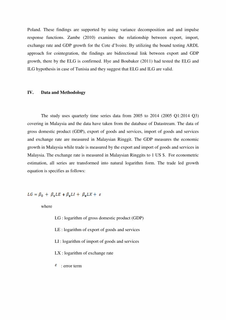
estimation, all series are transformed into natural logarithm form. The trade led growth
equation is specifies as follows:
where
LG : logarithm of gross domestic product (GDP)
LE : logarithm of export of goods and services
LI : logarithm of import of goods and services
LX : logarithm of exchange rate
: error term
Page 8
This study employs a time series technique, in particular, cointegration, error
correction modelling and variance decomposition in order to find empirical evidence of the
nature of relations between trade and economic growth. This method is favoured over the
traditional regression method for the following reasons. Firstly, regression techniques make
assumption about long run theoretical relationship among the variables and assume which
variables are leader and follower. However, the time series techniques test the long run
theoretical relationship among the variables and test the Granger-causality between variables.
Secondly, most finance variables are non-stationary. This means that performing
ordinary regression on the variables will render the results misleading, as statistical tests like
t-ratios and F statistics are not statistically valid when applied to non-stationary variables.
Performing regressions on the differenced form of these variables will solve one problem but
when variables are regressed in their differenced form, the long term trend is effectively
removed. Thus, the differenced regression variables only capture short term, cyclical or
seasonal effects. In other words, the regression in differenced forms is not really testing the
long term or theoretical relationships.
Thirdly, in traditional regression, the endogeneity and exogeneity of variables is pre-
determined by the researcher, usually on the basis of prevailing or a priori theories. However,
in cointegration techniques, the data will determine which variables are in fact endogenous
and exogenous. In other words, with regression, causality is presumed, whereas in
cointegration, it is empirically proven with the data.
V. Empirical Results
Table 1 shows the list of variables used in identifying the relationship between trade
and economic growth in Malaysia. The variables consist of GDP, export, import and
exchange rate. The variables are converted into natural logarithm to turn the series stationary
in variance and first difference of logarithm series to turn the series stationary in mean.
Page 9
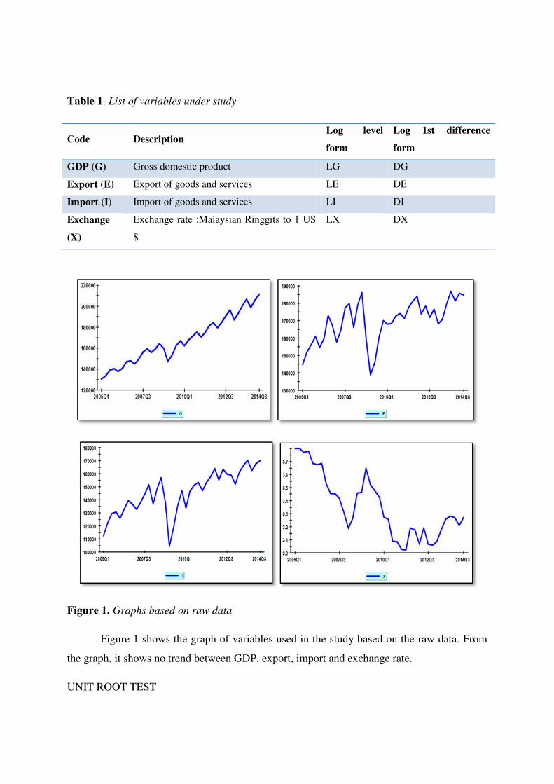
Table 1. List of variables under study
Code Description Log level
form
Log 1st difference
form
GDP (G) Gross domestic product LG DG
Export (E) Export of goods and services LE DE
Import (I) Import of goods and services LI DI
Exchange
(X)
Exchange rate :Malaysian Ringgits to 1 US
$
LX DX
Figure 1. Graphs based on raw data
Figure 1 shows the graph of variables used in the study based on the raw data. From
the graph, it shows no trend between GDP, export, import and exchange rate.
UNIT ROOT TEST
Page 10
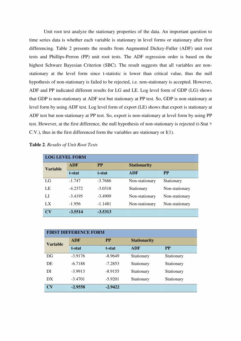
Unit root test analyze the stationary properties of the data. An important question to
time series data is whether each variable is stationary in level forms or stationary after first
differencing. Table 2 presents the results from Augmented Dickey-Fuller (ADF) unit root
tests and Phillips-Perron (PP) unit root tests. The ADF regression order is based on the
highest Schwarz Bayesian Criterion (SBC). The result suggests that all variables are non-
stationary at the level form since t-statistic is lower than critical value, thus the null
hypothesis of non-stationary is failed to be rejected, i.e. non-stationary is accepted. However,
ADF and PP indicated different results for LG and LE. Log level form of GDP (LG) shows
that GDP is non-stationary at ADF test but stationary at PP test. So, GDP is non-stationary at
level form by using ADF test. Log level form of export (LE) shows that export is stationary at
ADF test but non-stationary at PP test. So, export is non-stationary at level form by using PP
test. However, at the first difference, the null hypothesis of non-stationary is rejected (t-Stat >
C.V.), thus in the first differenced form the variables are stationary or I(1).
Table 2. Results of Unit Root Tests
LOG LEVEL FORM
Variable ADF PP Stationarity
t-stat t-stat ADF PP
LG -1.747 -3.7686 Non-stationary Stationary
LE -4.2372 -3.0318 Stationary Non-stationary
LI -3.4195 -3.4909 Non-stationary Non-stationary
LX -1.956 -1.1481 Non-stationary Non-stationary
CV -3.5514 -3.5313
FIRST DIFFERENCE FORM
Variable ADF PP Stationarity
t-stat t-stat ADF PP
DG -3.9176 -8.9649 Stationary Stationary
DE -6.7188 -7.2853 Stationary Stationary
DI -3.9913 -8.9155 Stationary Stationary
DX -3.4701 -5.9201 Stationary Stationary
CV -2.9558 -2.9422
Page 11
VAR ORDER
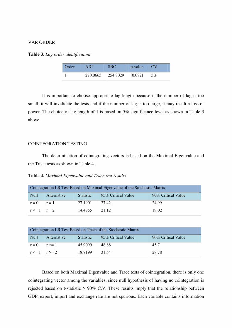
Table 3. Lag order identification
Order AIC SBC p-value CV
1 270.0665 254.8029 [0.082] 5%
It is important to choose appropriate lag length because if the number of lag is too
small, it will invalidate the tests and if the number of lag is too large, it may result a loss of
power. The choice of lag length of 1 is based on 5% significance level as shown in Table 3
above.
COINTEGRATION TESTING
The determination of cointegrating vectors is based on the Maximal Eigenvalue and
the Trace tests as shown in Table 4.
Table 4. Maximal Eigenvalue and Trace test results
Cointegration LR Test Based on Maximal Eigenvalue of the Stochastic Matrix
Null Alternative Statistic 95% Critical Value 90% Critical Value
r = 0 r = 1 27.1901 27.42 24.99
r <= 1 r = 2 14.4855 21.12 19.02
Cointegration LR Test Based on Trace of the Stochastic Matrix
Null Alternative Statistic 95% Critical Value 90% Critical Value
r = 0 r >= 1 45.9099 48.88 45.7
r <= 1 r >= 2 18.7199 31.54 28.78
Based on both Maximal Eigenvalue and Trace tests of cointegration, there is only one
cointegrating vector among the variables, since null hypothesis of having no cointegration is
rejected based on t-statistic > 90% C.V. These results imply that the relationship between
GDP, export, import and exchange rate are not spurious. Each variable contains information
Page 12
for the prediction of other variable. However, cointegration cannot tell the direction of
Granger-causality as to which variable is exogenous and which variable is endogenous, for
which the Vector Error Correction Modeling technique (VECM ) will be applied.
LONG-RUN STRUCTURAL MODELLING (LRSM)
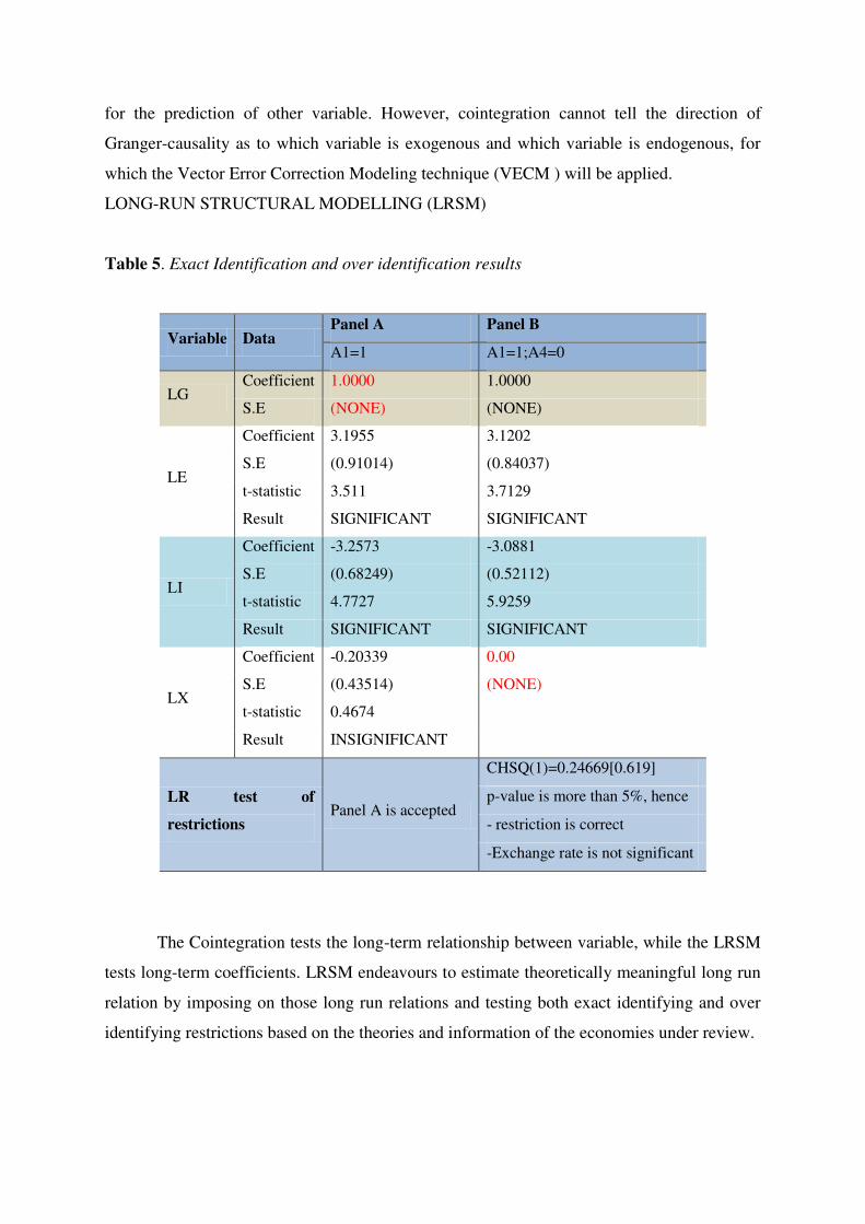
Table 5. Exact Identification and over identification results
Variable Data Panel A Panel B
A1=1 A1=1;A4=0
LG Coefficient 1.0000 1.0000
S.E (NONE) (NONE)
LE
Coefficient 3.1955 3.1202
S.E (0.91014) (0.84037)
t-statistic 3.511 3.7129
Result SIGNIFICANT SIGNIFICANT
LI
Coefficient -3.2573 -3.0881
S.E (0.68249) (0.52112)
t-statistic 4.7727 5.9259
Result SIGNIFICANT SIGNIFICANT
LX
Coefficient -0.20339 0.00
S.E (0.43514) (NONE)
t-statistic 0.4674
Result INSIGNIFICANT
LR test of
restrictions Panel A is accepted
CHSQ(1)=0.24669[0.619]
p-value is more than 5%, hence
- restriction is correct
-Exchange rate is not significant
The Cointegration tests the long-term relationship between variable, while the LRSM
tests long-term coefficients. LRSM endeavours to estimate theoretically meaningful long run
relation by imposing on those long run relations and testing both exact identifying and over
identifying restrictions based on the theories and information of the economies under review.
Page 13
Export and import of goods and services have significant impact on GDP since the t-
statistic is more than 2 but exchange rate is not significant in determining GDP. Testing over
identification for exchange rate shows that the restriction is correct since the CHSQ(1) is
more than 5% significance level.
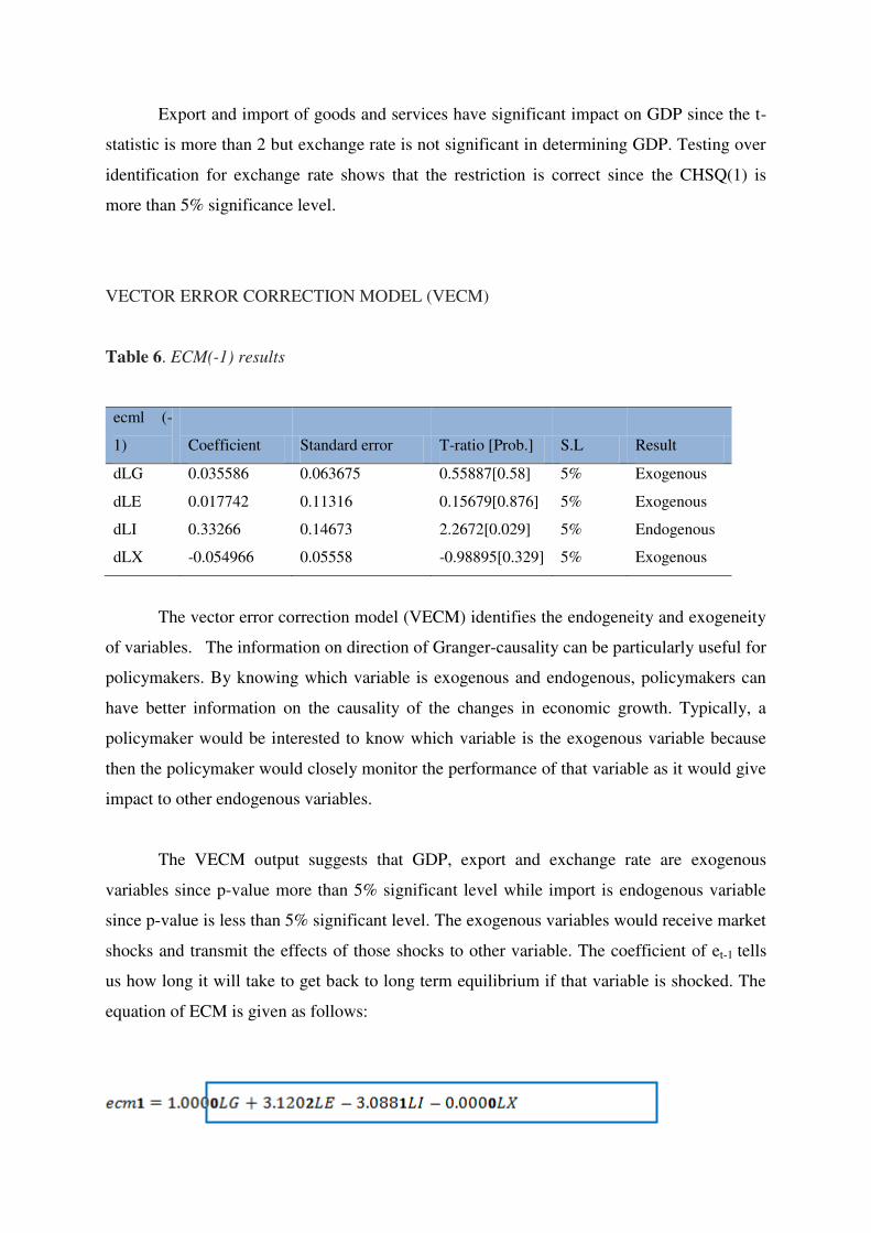
VECTOR ERROR CORRECTION MODEL (VECM)
Table 6. ECM(-1) results
ecml (-
1) Coefficient Standard error T-ratio [Prob.] S.L Result
dLG 0.035586 0.063675 0.55887[0.58] 5% Exogenous
dLE 0.017742 0.11316 0.15679[0.876] 5% Exogenous
dLI 0.33266 0.14673 2.2672[0.029] 5% Endogenous
dLX -0.054966 0.05558 -0.98895[0.329] 5% Exogenous
The vector error correction model (VECM) identifies the endogeneity and exogeneity
of variables. The information on direction of Granger-causality can be particularly useful for
policymakers. By knowing which variable is exogenous and endogenous, policymakers can
have better information on the causality of the changes in economic growth. Typically, a
policymaker would be interested to know which variable is the exogenous variable because
then the policymaker would closely monitor the performance of that variable as it would give
impact to other endogenous variables.
The VECM output suggests that GDP, export and exchange rate are exogenous
variables since p-value more than 5% significant level while import is endogenous variable
since p-value is less than 5% significant level. The exogenous variables would receive market
shocks and transmit the effects of those shocks to other variable. The coefficient of et-1 tells
us how long it will take to get back to long term equilibrium if that variable is shocked. The
equation of ECM is given as follows:
Page 14
VARIANCE DECOMPOSITIONS (VDCs)
Variance decompositions (VDCs) decompose the variance of forecast error of a
particular variable into proportions attributable to shocks in each variable in the system
including its own. The variable that is explained mostly by its own shocks is deemed to be
the most exogenous. Although the error-correction model has identified the endogeneity or
exogeneity of a variable, the generalized variance decomposition technique will assist in
determining the relative degree of endogeneity or exogeneity of the variables.
The VDCs and IRF serve as tools for evaluating the dynamic interactions and
strength of causal relations among variables in the system. There are two ways to identify the
relative exogeneity of variables. There are generalized approach and orthogonalized
approach. The generalized approach is preferred compared to the orthogonalized approach
because the orthogonalized approach is sensitive to the order of the variables in a VAR
system which determines the outcome of the results, whereas the generalized approach is
invariant to the ordering of variables in the VAR and produce one unique result.
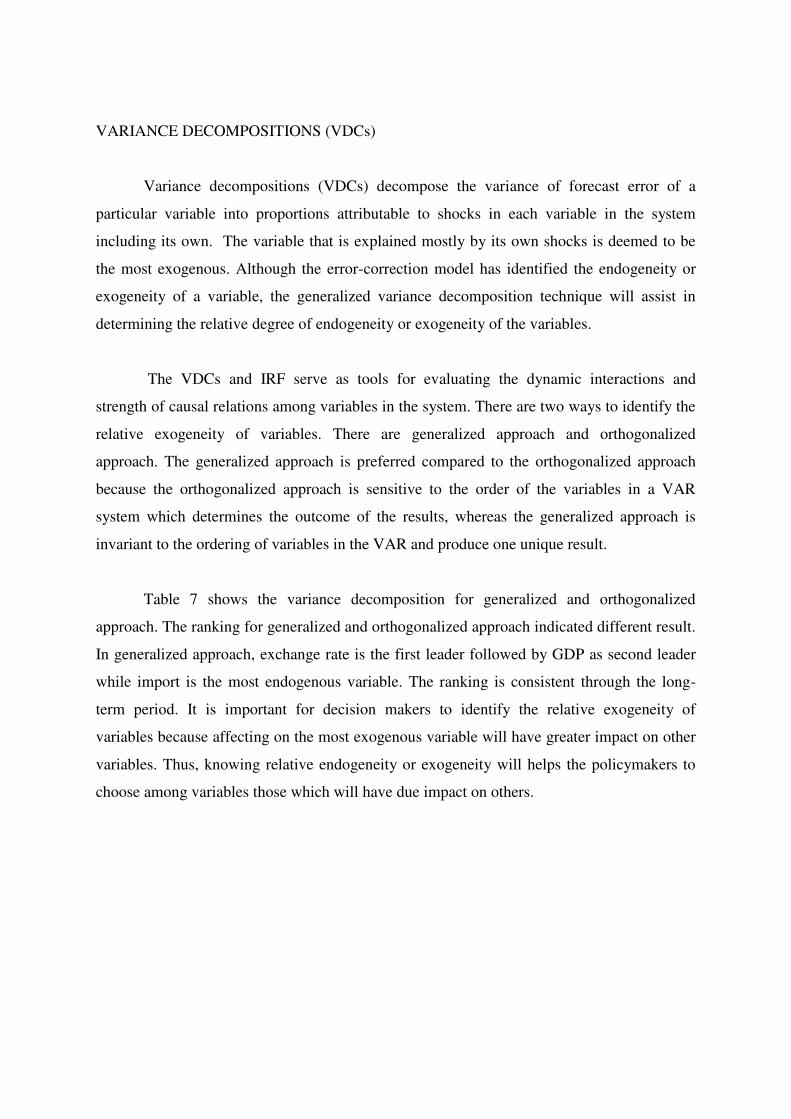
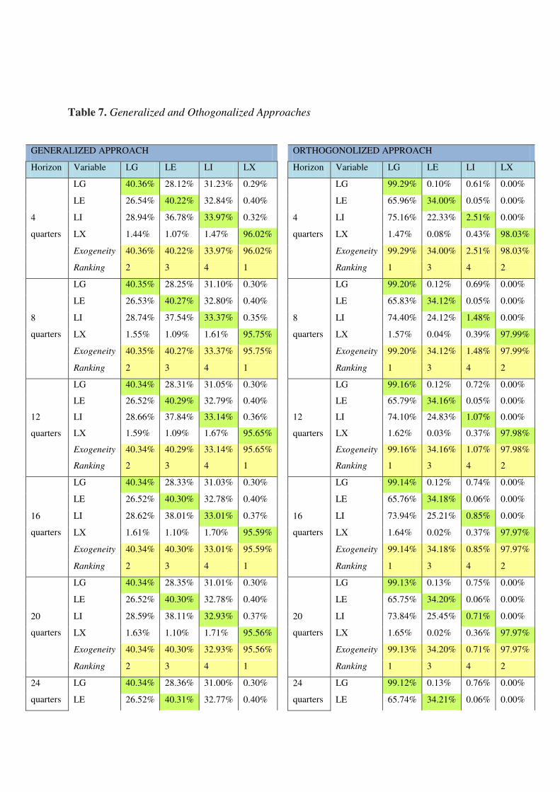
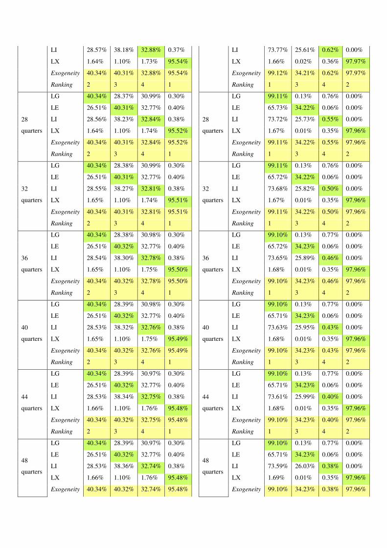
Table 7 shows the variance decomposition for generalized and orthogonalized
approach. The ranking for generalized and orthogonalized approach indicated different result.
In generalized approach, exchange rate is the first leader followed by GDP as second leader
while import is the most endogenous variable. The ranking is consistent through the long-
term period. It is important for decision makers to identify the relative exogeneity of
variables because affecting on the most exogenous variable will have greater impact on other
variables. Thus, knowing relative endogeneity or exogeneity will helps the policymakers to
choose among variables those which will have due impact on others.
Page 15
Table 7. Generalized and Othogonalized Approaches
GENERALIZED APPROACH
ORTHOGONOLIZED APPROACH
Horizon Variable LG LE LI LX
Horizon Variable LG LE LI LX
4
quarters
LG 40.36% 28.12% 31.23% 0.29%
4
quarters
LG 99.29% 0.10% 0.61% 0.00%
LE 26.54% 40.22% 32.84% 0.40%
LE 65.96% 34.00% 0.05% 0.00%
LI 28.94% 36.78% 33.97% 0.32%
LI 75.16% 22.33% 2.51% 0.00%
LX 1.44% 1.07% 1.47% 96.02%
LX 1.47% 0.08% 0.43% 98.03%
Exogeneity 40.36% 40.22% 33.97% 96.02%
Exogeneity 99.29% 34.00% 2.51% 98.03%
Ranking 2 3 4 1
Ranking 1 3 4 2
8
quarters
LG 40.35% 28.25% 31.10% 0.30%
8
quarters
LG 99.20% 0.12% 0.69% 0.00%
LE 26.53% 40.27% 32.80% 0.40%
LE 65.83% 34.12% 0.05% 0.00%
LI 28.74% 37.54% 33.37% 0.35%
LI 74.40% 24.12% 1.48% 0.00%
LX 1.55% 1.09% 1.61% 95.75%
LX 1.57% 0.04% 0.39% 97.99%
Exogeneity 40.35% 40.27% 33.37% 95.75%
Exogeneity 99.20% 34.12% 1.48% 97.99%
Ranking 2 3 4 1
Ranking 1 3 4 2
12
quarters
LG 40.34% 28.31% 31.05% 0.30%
12
quarters
LG 99.16% 0.12% 0.72% 0.00%
LE 26.52% 40.29% 32.79% 0.40%
LE 65.79% 34.16% 0.05% 0.00%
LI 28.66% 37.84% 33.14% 0.36%
LI 74.10% 24.83% 1.07% 0.00%
LX 1.59% 1.09% 1.67% 95.65%
LX 1.62% 0.03% 0.37% 97.98%
Exogeneity 40.34% 40.29% 33.14% 95.65%
Exogeneity 99.16% 34.16% 1.07% 97.98%
Ranking 2 3 4 1
Ranking 1 3 4 2
16
quarters
LG 40.34% 28.33% 31.03% 0.30%
16
quarters
LG 99.14% 0.12% 0.74% 0.00%
LE 26.52% 40.30% 32.78% 0.40%
LE 65.76% 34.18% 0.06% 0.00%
LI 28.62% 38.01% 33.01% 0.37%
LI 73.94% 25.21% 0.85% 0.00%
LX 1.61% 1.10% 1.70% 95.59%
LX 1.64% 0.02% 0.37% 97.97%
Exogeneity 40.34% 40.30% 33.01% 95.59%
Exogeneity 99.14% 34.18% 0.85% 97.97%
Ranking 2 3 4 1
Ranking 1 3 4 2
20
quarters
LG 40.34% 28.35% 31.01% 0.30%
20
quarters
LG 99.13% 0.13% 0.75% 0.00%
LE 26.52% 40.30% 32.78% 0.40%
LE 65.75% 34.20% 0.06% 0.00%
LI 28.59% 38.11% 32.93% 0.37%
LI 73.84% 25.45% 0.71% 0.00%
LX 1.63% 1.10% 1.71% 95.56%
LX 1.65% 0.02% 0.36% 97.97%
Exogeneity 40.34% 40.30% 32.93% 95.56%
Exogeneity 99.13% 34.20% 0.71% 97.97%
Ranking 2 3 4 1
Ranking 1 3 4 2
24
quarters
LG 40.34% 28.36% 31.00% 0.30%
24
quarters
LG 99.12% 0.13% 0.76% 0.00%
LE 26.52% 40.31% 32.77% 0.40%
LE 65.74% 34.21% 0.06% 0.00%
Page 16
LI 28.57% 38.18% 32.88% 0.37%
LI 73.77% 25.61% 0.62% 0.00%
LX 1.64% 1.10% 1.73% 95.54%
LX 1.66% 0.02% 0.36% 97.97%
Exogeneity 40.34% 40.31% 32.88% 95.54%
Exogeneity 99.12% 34.21% 0.62% 97.97%
Ranking 2 3 4 1
Ranking 1 3 4 2
28
quarters
LG 40.34% 28.37% 30.99% 0.30%
28
quarters
LG 99.11% 0.13% 0.76% 0.00%
LE 26.51% 40.31% 32.77% 0.40%
LE 65.73% 34.22% 0.06% 0.00%
LI 28.56% 38.23% 32.84% 0.38%
LI 73.72% 25.73% 0.55% 0.00%
LX 1.64% 1.10% 1.74% 95.52%
LX 1.67% 0.01% 0.35% 97.96%
Exogeneity 40.34% 40.31% 32.84% 95.52%
Exogeneity 99.11% 34.22% 0.55% 97.96%
Ranking 2 3 4 1
Ranking 1 3 4 2
32
quarters
LG 40.34% 28.38% 30.99% 0.30%
32
quarters
LG 99.11% 0.13% 0.76% 0.00%
LE 26.51% 40.31% 32.77% 0.40%
LE 65.72% 34.22% 0.06% 0.00%
LI 28.55% 38.27% 32.81% 0.38%
LI 73.68% 25.82% 0.50% 0.00%
LX 1.65% 1.10% 1.74% 95.51%
LX 1.67% 0.01% 0.35% 97.96%
Exogeneity 40.34% 40.31% 32.81% 95.51%
Exogeneity 99.11% 34.22% 0.50% 97.96%
Ranking 2 3 4 1
Ranking 1 3 4 2
36
quarters
LG 40.34% 28.38% 30.98% 0.30%
36
quarters
LG 99.10% 0.13% 0.77% 0.00%
LE 26.51% 40.32% 32.77% 0.40%
LE 65.72% 34.23% 0.06% 0.00%
LI 28.54% 38.30% 32.78% 0.38%
LI 73.65% 25.89% 0.46% 0.00%
LX 1.65% 1.10% 1.75% 95.50%
LX 1.68% 0.01% 0.35% 97.96%
Exogeneity 40.34% 40.32% 32.78% 95.50%
Exogeneity 99.10% 34.23% 0.46% 97.96%
Ranking 2 3 4 1
Ranking 1 3 4 2
40
quarters
LG 40.34% 28.39% 30.98% 0.30%
40
quarters
LG 99.10% 0.13% 0.77% 0.00%
LE 26.51% 40.32% 32.77% 0.40%
LE 65.71% 34.23% 0.06% 0.00%
LI 28.53% 38.32% 32.76% 0.38%
LI 73.63% 25.95% 0.43% 0.00%
LX 1.65% 1.10% 1.75% 95.49%
LX 1.68% 0.01% 0.35% 97.96%
Exogeneity 40.34% 40.32% 32.76% 95.49%
Exogeneity 99.10% 34.23% 0.43% 97.96%
Ranking 2 3 4 1
Ranking 1 3 4 2
44
quarters
LG 40.34% 28.39% 30.97% 0.30%
44
quarters
LG 99.10% 0.13% 0.77% 0.00%
LE 26.51% 40.32% 32.77% 0.40%
LE 65.71% 34.23% 0.06% 0.00%
LI 28.53% 38.34% 32.75% 0.38%
LI 73.61% 25.99% 0.40% 0.00%
LX 1.66% 1.10% 1.76% 95.48%
LX 1.68% 0.01% 0.35% 97.96%
Exogeneity 40.34% 40.32% 32.75% 95.48%
Exogeneity 99.10% 34.23% 0.40% 97.96%
Ranking 2 3 4 1
Ranking 1 3 4 2
48
quarters
LG 40.34% 28.39% 30.97% 0.30%
48
quarters
LG 99.10% 0.13% 0.77% 0.00%
LE 26.51% 40.32% 32.77% 0.40%
LE 65.71% 34.23% 0.06% 0.00%
LI 28.53% 38.36% 32.74% 0.38%
LI 73.59% 26.03% 0.38% 0.00%
LX 1.66% 1.10% 1.76% 95.48%
LX 1.69% 0.01% 0.35% 97.96%
Exogeneity 40.34% 40.32% 32.74% 95.48%
Exogeneity 99.10% 34.23% 0.38% 97.96%
Page 17
Ranking 2 3 4 1
Ranking 1 3 4 2
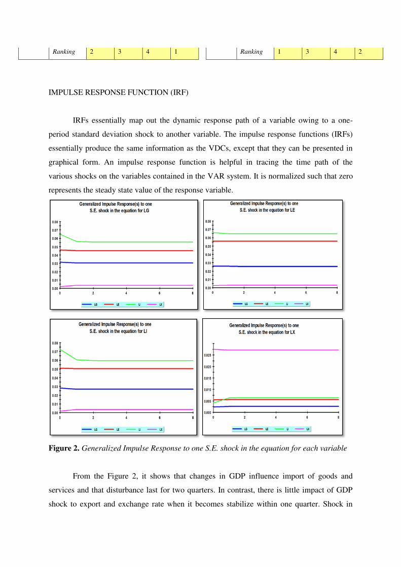
IMPULSE RESPONSE FUNCTION (IRF)
IRFs essentially map out the dynamic response path of a variable owing to a one-
period standard deviation shock to another variable. The impulse response functions (IRFs)
essentially produce the same information as the VDCs, except that they can be presented in
graphical form. An impulse response function is helpful in tracing the time path of the
various shocks on the variables contained in the VAR system. It is normalized such that zero
represents the steady state value of the response variable.
Figure 2. Generalized Impulse Response to one S.E. shock in the equation for each variable
From the Figure 2, it shows that changes in GDP influence import of goods and
services and that disturbance last for two quarters. In contrast, there is little impact of GDP
shock to export and exchange rate when it becomes stabilize within one quarter. Shock in
Page 18
export has more impact on GDP as compared to import and exchange rate when it become
normalize within two quarters but it takes one quarter to normalize for import and exchange
rate.
Shock in import of goods and services have same impact for GDP, export and
exchange rate which will normalize within one quarter. This result supports that import is
weak or endogenous variable because it does not give strong impact to other variables.
Exchange rate change has strong impact on import lasting for about two quarters, but slight
influence on GDP and export which will normalize within one quarter. Exchange rate is the
most leading variable by looking at the scale of the graphs and import is the most endogenous
which is consistent with the findings from VECM and VDC steps.
The trade openness of a country will depends on the exchange rate of a country. The
policymakers will make decision on the export and import of goods and services based on
exchange rate because changes in exchange rate will give impact on GDP, import and export
as exchange rate is the leader variable.
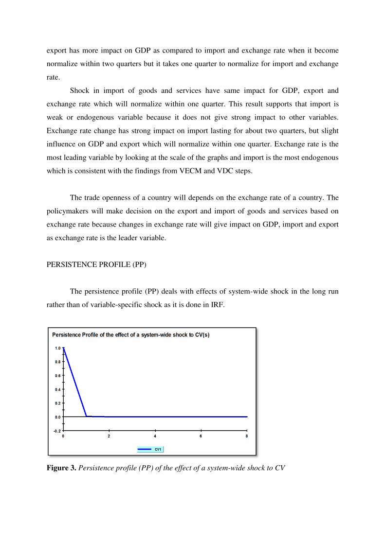
PERSISTENCE PROFILE (PP)
The persistence profile (PP) deals with effects of system-wide shock in the long run
rather than of variable-specific shock as it is done in IRF.
Figure 3. Persistence profile (PP) of the effect of a system-wide shock to CV
Page 19
The results indicate that if the long-term convergence between the variables is
disturbed by any shocks, it will take about two quarters to restore the equilibrium.
VI. Conclusions and Policy Implications
This study examines empirically the causal links between export, import, exchange
rate and economic growth in Malaysia by conducting multivariate time series. Economic
theory suggests that both the export and import sectors can contribute to economic growth.
However, most of previous researches have only focused on the role of export sector while
ignoring the potential growth contribution of the import sector. This study is concluded to
three key findings on the basis of empirical evidence. First, there is bidirectional causal
relationship exists between export and economic growth where export leads economic growth
and economic growth leads export. This finding confirms the validity of ELG and GLE
hypothesis. This finding is equal to the empirical findings of Mah (2005) in case of China.
Secondly, the bidirectional relationship between import and economic growth
confirms the validity of ILG and GLI hypothesis. The present empirical result is equal with
the earlier findings of Sato and Fukushige (2007) in case of North Korea. Thirdly, the result
indicates the bidirectional long-run association between export and import. In summary, the
findings from this study confirm that the exclusion of imports and the singular focus on the
role of exports as the engine of growth may be misleading. However, the economic growth is
the second leader compared to exchange rate which is the most exogenous. It means that, any
shock in exchange rate will impact the export, import and economic growth.
The empirical findings are very helpful for trade policymakers. There are several
policy implications of this finding in Malaysia and other developing countries. First, export
promotion as a strategy for economic growth would only be partially effective if import
restrictions are maintained. Second, import openness is very important to economic growth as
it complements the role of exports by serving as a supply of intermediate production inputs
needed in the export sector. Third, developing economies with limited technological
Page 20
endowment could benefit from access to foreign technology and knowledge from developed
countries via imports. Finally, it is recommended for the future empirical research focusing
on the trade and foreign direct investment in stimulating economic growth. It may be useful
to extend the analytical framework used in this study to other developing countries.
References
Ahmad, J. & Harnhirun, S. (1995) “Unit roots and cointegration in estimating causality
between exports and economic growth: empirical evidence from the ASEAN
countries”.Economics Letters. 49(3). p. 329-34.
Awokuse, T. O. (2006) Export-led growth and the Japanese economy: evidence from VAR
and directed acyclic graphs. Applied Economics. 38.p. 593–602.
Awokuse, T.O. (2007) “Causality between exports, imports, and economic growth: evidence
from transition economies”. Economics Letters.94(3). p. 389-95.
Awokuse, T. O. (2008) Trade openness and economic growth: is growth export-led or
import-led? Applied Economics. 40. p. 161-173
Bahmani-Oskooee, M. & Alse, J. (1993) “Export growth and economic growth: an
application of cointegration and error correction modelling”, Journal of Developing
Areas. 27(4). p. 535-42.
Faridul, I., Qazi, M.A.H & Muhammad, S. (2012) Import-economic growth nexus: ARDL
approach to cointegration. Journal of Chinese Economic and Foreign Trade
Studies.5(3). p. 194-214
Giles, J. A. & Williams, C. L. (2000) Export-led growth: a survey of the empirical literature
and some noncausality results. Journal of International Trade and Economic
Development. 9.p. 261–337.
Hye, Q.M.A. & Boubaker, H.B.H. (2011) “Exports, imports and economic growth: an
empirical analysis of Tunisia”The IUP Monetary Economics. 9(1).p. 6-21.
Liu, X., Chang, S. & Peter, S.(2009) Trade, foreign direct investment and economic growth
in Asian economies. Applied Economics. 41. p. 1603-1612
Mah, J.S. (2005) “Export expansion, economic growth and causality in China”. Applied
Economics Letters.12(2). p. 105-7.
Mahadevan, R. & Suardi, S. (2008) “A dynamic analysis of the impact of uncertainty on
Page 21
import-and/or export-led growth: the experience of Japan and the Asian tigers”.
Japan and the World Economy. 20(2). p. 155-74.
Mazumdar, J. (2002) Imported machinery and growth in LDCs. Journal of Development
Economics. 65.p.209–24.
McNab, R.M. & Moore, R.E. (1998) “Trade policy, export expansion, human capital and
growth”. Journal of International Trade and Economic Development. 7(2).
p 237-56.
Qazi, M. A. H. (2012) Exports, imports and economic growth in China: an ARDL analysis. .
Journal of Chinese Economic and Foreign Trade Studies.5(1).p.42-55
Ramos, F.F.R. (2001) “Exports, imports, and economic growth in Portugal: evidence from
causality and cointegration analysis”. Journal of Economic Modeling.18(4).
p. 613-23.
Sato, S. & Fukushige, M. (2007) “The end of import-led growth? North Korean evidence”.
available at: www2.econ.osaka-u.ac.jp/library/global/dp/0738.pdf
Thangavelu, S.M. & Rajaguru, G. (2004) “Is there an export or import-led productivity
growth in rapidly developing Asian countries? A multivariate VAR analysis”.
Applied Economics. 36(10). p. 1083-93.