econstor www.econstor.eu Der Open-Access-Publikationsserver der ZBW – Leibniz-Informationszentrum Wirtschaft The Open Access Publication Server of the ZBW – Leibniz Information Centre for Economics Standard-Nutzungsbedingungen: Die Dokumente auf EconStor dürfen zu eigenen wissenschaftlichen Zwecken und zum Privatgebrauch gespeichert und kopiert werden. Sie dürfen die Dokumente nicht für öffentliche oder kommerzielle Zwecke vervielfältigen, öffentlich ausstellen, öffentlich zugänglich machen, vertreiben oder anderweitig nutzen. Sofern die Verfasser die Dokumente unter Open-Content-Lizenzen (insbesondere CC-Lizenzen) zur Verfügung gestellt haben sollten, gelten abweichend von diesen Nutzungsbedingungen die in der dort genannten Lizenz gewährten Nutzungsrechte. Terms of use: Documents in EconStor may be saved and copied for your personal and scholarly purposes. You are not to copy documents for public or commercial purposes, to exhibit the documents publicly, to make them publicly available on the internet, or to distribute or otherwise use the documents in public. If the documents have been made available under an Open Content Licence (especially Creative Commons Licences), you may exercise further usage rights as specified in the indicated licence. zbw Leibniz-Informationszentrum Wirtschaft Leibniz Information Centre for Economics Felbermayr, Gabriel J.; Heiland, Inga; Yalcin, Erdal Working Paper Mitigating liquidity constraints: Public export credit guarantees in Germany CESifo Working Paper: Trade Policy, No. 3908 Provided in Cooperation with: Ifo Institute – Leibniz Institute for Economic Research at the University of Munich Suggested Citation: Felbermayr, Gabriel J.; Heiland, Inga; Yalcin, Erdal (2012) : Mitigating liquidity constraints: Public export credit guarantees in Germany, CESifo Working Paper: Trade Policy, No. 3908 This Version is available at: http://hdl.handle.net/10419/62325
Transcript
econstor www.econstor.eu
Der Open-Access-Publikationsserver der ZBW – Leibniz-Informationszentrum WirtschaftThe Open Access Publication Server of the ZBW – Leibniz Information Centre for Economics
Standard-Nutzungsbedingungen:
Die Dokumente auf EconStor dürfen zu eigenen wissenschaftlichenZwecken und zum Privatgebrauch gespeichert und kopiert werden.
Sie dürfen die Dokumente nicht für öffentliche oder kommerzielleZwecke vervielfältigen, öffentlich ausstellen, öffentlich zugänglichmachen, vertreiben oder anderweitig nutzen.
Sofern die Verfasser die Dokumente unter Open-Content-Lizenzen(insbesondere CC-Lizenzen) zur Verfügung gestellt haben sollten,gelten abweichend von diesen Nutzungsbedingungen die in der dortgenannten Lizenz gewährten Nutzungsrechte.
Terms of use:
Documents in EconStor may be saved and copied for yourpersonal and scholarly purposes.
You are not to copy documents for public or commercialpurposes, to exhibit the documents publicly, to make thempublicly available on the internet, or to distribute or otherwiseuse the documents in public.
If the documents have been made available under an OpenContent Licence (especially Creative Commons Licences), youmay exercise further usage rights as specified in the indicatedlicence.
zbw Leibniz-Informationszentrum WirtschaftLeibniz Information Centre for Economics
Felbermayr, Gabriel J.; Heiland, Inga; Yalcin, Erdal
Working Paper
Mitigating liquidity constraints: Public export creditguarantees in Germany
CESifo Working Paper: Trade Policy, No. 3908
Provided in Cooperation with:Ifo Institute – Leibniz Institute for Economic Research at the University ofMunich
Suggested Citation: Felbermayr, Gabriel J.; Heiland, Inga; Yalcin, Erdal (2012) : Mitigatingliquidity constraints: Public export credit guarantees in Germany, CESifo Working Paper: TradePolicy, No. 3908
This Version is available at:http://hdl.handle.net/10419/62325
Mitigating Liquidity Constraints: Public Export Credit Guarantees in Germany
Gabriel J. Felbermayr Inga Heiland Erdal Yalcin
CESIFO WORKING PAPER NO. 3908 CATEGORY 8: TRADE POLICY
AUGUST 2012
An electronic version of the paper may be downloaded • from the SSRN website: www.SSRN.com • from the RePEc website: www.RePEc.org
• from the CESifo website: Twww.CESifo-group.org/wp T
Mitigating Liquidity Constraints: Public Export Credit Guarantees in Germany
Abstract
Reportedly, firms often find it impossible to finance large and long-term projects despite positive net present values. Should governments step in and can their assistance be effective? This paper studies the case of public export credit guarantees in Germany. Covering the default risk of exporters’ foreign customers, the policy is supposed to enable funding of international business opportunities that would otherwise remain unexploited. Using German firm-level data covering the universe of publicly insured firms for the years 2000 to 2010, this study tests for the causal effect of guarantees on sales and employment. It employs a difference-in-differences strategy combined with a matching approach, to create an appropriate control group of untreated firms. It finds that guarantees increase firm-level sales and employment on average by about 4.5 and 3.0 percentage points, respectively. During the financial crisis of 2008/09, effects turn out larger. These findings suggest the presence of credit constraints and provide an argument justifying the observed government intervention.
July 2012 We are grateful to Petra Dithmer and Lars Ponterlitschek from Euler Hermes, Oliver Hunke and Matthias Köhler from the German Federal Ministry of Economics and Technology. Special thanks go to Heike Mittelmeier and Christian Seiler from the Munich Economics and Business Data Center (EBDC) for their invaluable assistance with data.
1 Introduction
By now it is widely accepted that credit constraints can limit firm growth (Rajan and Zingales,1998; Fisman and Love, 2007). Constraints are more likely binding when projects are long-term, large, hard to monitor, and risky. This fact begs an important but tricky public financequestion: should governments help firms obtaining credit?
Banerjee and Duflo (2012) argue that, in the presence of a public credit program, un-constrained firms would simply substitute public for private instruments, as the former maybe less costly than the latter, leaving the level of economic activity unchanged. Credit con-strained firms, instead, would expand their activities. We apply this argument to the caseof public export credit guarantees. Auboin (2007) and Jean-Pierre and Farole (2009) findthat about 80 percent of all exporters make use of some form of trade finance such as exportcredit insurance.1 However, for certain export destinations and large volumes appropriateinsurance instruments seem unavailable, which makes it difficult for exporters to refinanceinternational business activities. For this reason, an increasing number of countries issuepublic export credit guarantees, supposedly enabling firms to obtain credit to finance exporttransactions that would have not been feasible otherwise.2
Egger and Url (2006) estimate a gravity-model for Austrian exports on the industry level.3
Felbermayr and Yalcin (2011) go beyond measuring direct export promoting effects. Theyuse industry-level export data for Germany to show that public guarantees indeed seem toincrease exports by alleviating financial frictions encountered by exporting firms.4 To date,an analysis of firm-level data is still missing. Filling this gap, this paper studies the firm-level performance effects of export credit guarantees underwritten by the Federal Republicof Germany.
Working with firm-level data has several advantages. First, it allows to deal with thenon-random selection of firms into public insurance programs, thereby allowing a causalinterpretation of the results. There are several reasons to belief that assignment of treatmentis not random. More successful firms may be better suited in simultaneously obtaininglarger export contracts and securing public support. If this is the case, estimations based
1Antràs and Foley (2011) develop a theory of trade finance and provide evidence for a large single firmin the US poultry industry.
2Berne Union, the leading international association which brings together 48 national export credit agen-cies (ECAs), reckons that over US $1.4 trillion worth of export were covered by credit guarantees in 2010,facilitating about 10% of world trade (see Berne Union (2010)).
3Moser et al. (2008) run a similar exercise on aggregate data for Germany while Janda et al. (2012) repeatthe exercise for Czech data.
4Earlier important theoretical and empirical contributions include Fleisig and Hill (1984), Abraham andDewit (2000), Dewit (2001).
1
on ordinary least squares may yield spurious correlations. Similarly it is conceivable, thatthe government grants public insurance as an award for their export success. This wouldimply reverse causation. We deal with these possibilities by applying a matching approach(Rosenbaum and Rubin, 1983; Imbens, 2004; Abadie, 2005).5 More precisely, in this paperwe use a semi-parametric matching estimator proposed by Abadie and Imbens (2011) andcombine it with a difference-in-difference strategy following Heckman et al. (1997) to betteraccount for unobservable but time-invariant firm characteristics that may otherwise confoundthe relation between public insurance and firm performance. Existing macro studies have notbeen able to convincingly address this issue.
Second, our focus on firm-level data allows us to work with a larger array of variables that,presumably, should be affected by public guarantees such as total sales and employment, butalso value added or wages. Indeed, politicians regularly rationalize the public underwritingof export credit risk on the basis of alleged positive employment effects. While we are not at-tempting a full-fledged general equilibrium analysis of the welfare effects of these guarantees,in the presence of constraints, positive sales and employment effects are necessary conditionsfor those to arise (Banerjee and Duflo, 2012). Focusing on total sales rather than exportsensures that what we capture is not just a reallocation of sales induced by moral hazard, inthe sense that firms under public insurance schemes reallocate sales from less risky domesticand foreign markets to more risky ones, but a real increase in aggregate activity.
This paper draws on a data base that contains the universe of firms located in Germanythat have received public credit guarantees in the period 2000 to 2010. The data is providedby Euler-Hermes, a private consortium that administers public export credit guarantees onbehalf of the German government. Any losses or profits are consolidated into the federalbudget. Germany is an interesting case to study. First, it is a major exporting country,rivalled only by China and the US.6 Also, Euler-Hermes turns out to be one of the largestpublic export insurers. Total exposure to short-term export credit risk totalled 61 billiondollar for the US, 60 billion dollars for Germany, and 39 billion for China.7 So, the case ofGermany is of key interest.
Our paper relates to an increasing body of theoretical and empirical literature analyzingthe role of financial frictions for exporters’ performance in light of the dramatic drop ofglobal export flows during the latest financial market crises. Amiti and Weinstein (2009)illustrate the importance of bank health for firms’ export activities. Chor and Manova (2011)additionally show that sectors with greater external finance structure experienced a stronger
5For studies that have treated related problems of firm selection with matching methods see e.g. Wagner(2011) and Chari et al. (2009).
6From 2003 to 2008, Germany was actually the largest exporter in the world.7According to statistics published by Berne Union (2012).
2
drop in sales during the financial crises. Paravisini et al. (2011) use matched data fromPeru to show that about 15% of the total decline in exports was due to credit shortages.One conclusion emerging from this literature is that financial market frictions restrain cross-border sales. Felbermayr and Yalcin (2011) build on these insights and analyze the effectsof public export schemes in the presence of financial constraints based on industry-leveldata. Following Chor and Manova (2011), the authors show that German export creditguarantees have helped mitigate the liquidity crunch during the financial crisis especiallyin financially vulnerable sectors. While their study provides new results with respect tothe interplay of export credit guarantees and sectoral financial frictions, it does not allow acausal interpretation of the estimates. Following this strand of literature, we interpret thecrisis of 2008/2009 as an exogenous shock to the availability of finance. This allows to analyzewhether public guarantees indeed help mitigate financial frictions.
The empirical results in our paper suggest the following new conclusions. Firms receivingexport credit guarantees experience 4 to 4.5 percentage points higher sales growth comparedto similar firms without credit guarantee treatment in the year of the grant of a guarantee(average treatment effect on the treated firms, ATT). Employment growth is on average 2.5 to3 percentage points higher for treated firms. Given that firms cover on average 6.6 percent oftheir yearly sales, the resulting magnitudes are plausible. The estimated treatment effects arevery robust across different specifications and our results from a placebo treatment analysisstrongly support their credibility.
The remainder of the paper is organized as follows. Section 2 describes export creditguarantees in Germany and provides some descriptive evidence. In Section 3 we brieflypresent an overview of our firm level data. Section 4 motivates and explains our empiricalstrategy and in Section 5 we discuss our choice of matching variables. In Section 6 we presentour results and discuss them. Section 7 concludes.
2 German Export Credit Guarantees
The German government guarantees certain export credit claims of firms located in Ger-many. Guarantees are issued by a consortium made up by PriceWaterhouseCoopers-AGand the Hermes-Kreditversicherungs-AG on behalf of the Republic of Germany. Therefore,German export credit guarantees are also referred to as “Hermes guarantees”.8 Budgetaryresponsibility for this instrument lies with the Federal Government that decides on generalcoverage policy and the granting of guarantees in an Interministerial Committee (IMC). Due
8In ancient Greek mythology, Hermes, the son of Zeus and the Pleiade Maia, was the messenger of thegods to humans, and the protector of shepherds and cowherds, thieves, orators and wit, literature and poets,athletics and sports, weights and measures, invention, and of commerce in general.
3
to the public character of Hermes guarantees, profits and losses made by the consortium aredirectly incorporated into the German federal budget. Eligibility of countries, sectors, andcosts for coverage is defined in a “gentlemen’s agreement” amongst OECD member countriesalso known as the OECD Arrangement or the OECD consensus.9 The OECD consensus isimportant because under WTO rules, “the provision by governments (or special institutionscontrolled by governments) of export credit guarantee or insurance programmes” qualifies asexport subsidies and is, thus, outlawed. However, the WTO Agreement on Subsidies andCountervailing Measures exempts those schemes if at least twelve GATT members take partin an “international undertaking on official export credits” that regulates the use of thoseguarantees.10
In compliance with the OECD Arrangement the German export credit guarantee systemoffers three instruments. The first and quantitatively most important is the “Einzeldeck-ung” (EZD) which refers to single, well-defined projects (transactions) for specific sectorsand countries. The second instrument, the “Ausfuhrpauschalgewährleistung” (APG) simul-taneously covers several importers, potentially in different countries. The last instrument,“revolving guarantees”, is negligible as it represents less than 2 percent of total coverage. Thekey objective of Hermes guarantees is to support exporters by assuming payment default riskfor certain export transactions against the payment of a premium, which depends on coun-try risk as classified by the OECD Arrangement.11 Export credit claims against customerslocated in the European Union (EU) or other OECD countries (except Chile, Israel, Mexico,South Korea, and Turkey) with contract durations of less than 24 months are assumed tobe marketable and therefore cannot be publicly insured.12 Contracts of longer duration canprincipally be insured for all countries, subject to an array of conditions. For example, Ger-man value added must be at least 70% of the total sales contract to be insured or the valueadded content of the destination country must not exceed 23%.
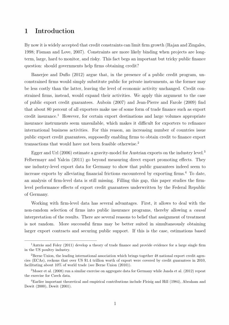
Table I shows the time behavior of German exports and the volume of Hermes guaranteesover the last ten years. Aggregate exports almost doubled between 2000 and 2008 from500 billion to almost one trillion Euros. During that period, the issuance of public exportcredit guarantees first declined from 3.3 to 1.8 percent of total exports in 2007. Followingthe collapse of financial markets after the Lehman Brothers bankruptcy, the share of exports
9Current participants to the arrangement are: Australia, Canada, the European Union, Japan, Korea,New Zealand, Norway, Switzerland and the United States.
10WTO Agreement on Subsidies and Countervailing Measures, Annex I, articles j and k.11The classification is publicly available and known as Country Risk Classifications of the Participants to
the Arrangement on Officially Supported Export Credits. It groups countries into eight groups according totheir riskiness with 0 as the lowest risk level and 7 as the highest one.
12Due to the financial crisis in 2008/09 the list of eligible countries was extended during the period 2009-2012.
4
Table I: German Exports and Hermes Guarantees, 2000-2010
Notes: Yearly German exports and GNP data are from the Federal Statistical Office of Germany. Aggregate Hermes guaranteesrepresent the yearly sum of EZD, APG and revolving guarantees. The data was provided by Euler-Hermes. Coverage is calculatedas sum of Hermes guarantees over Exports. a) ifo Credit Constraint Indicator: share of surveyed manufacturing firms indicatingthat credit access is “restricted”.
covered increased again to 3.4 percent as of 2010. This reflects the substitution of public forprivate insurance and points towards a possible mitigating effect of public guarantees in theglobal trade collapse of 2008.13
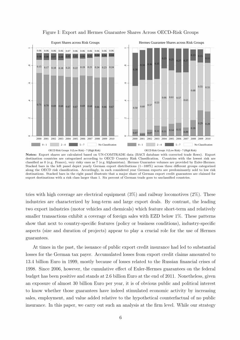
Public export credit guarantees play an important role in emerging economies charac-terized by risky business environments. Figure I illustrates the distribution of exports andHermes guarantees across different OECD country risk classes over time.14 In all years,countries in the middle risk categories (categories 2 to 4, including emerging economies likeChina, Brazil and India) have absorbed 50 to 68 percent of Hermes guarantees, while onlyaccounting for 15 to 24 percent of German exports. Middle and high risk countries togetheraccount for about 90 percent of Hermes guarantees before the crisis, but only for about onequarter of German exports. Low risk countries absorb more than two thirds of German ex-ports but, before the crisis, account for not more than 15 percent of Hermes guarantees. Inthe aftermath of the global financial crisis, when OECD countries such as Greece becometemporarily eligible for Hermes coverage, that share rose to 29 percent.
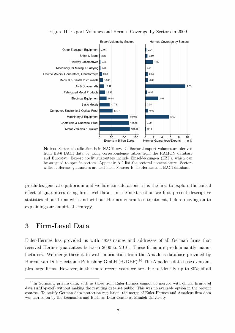
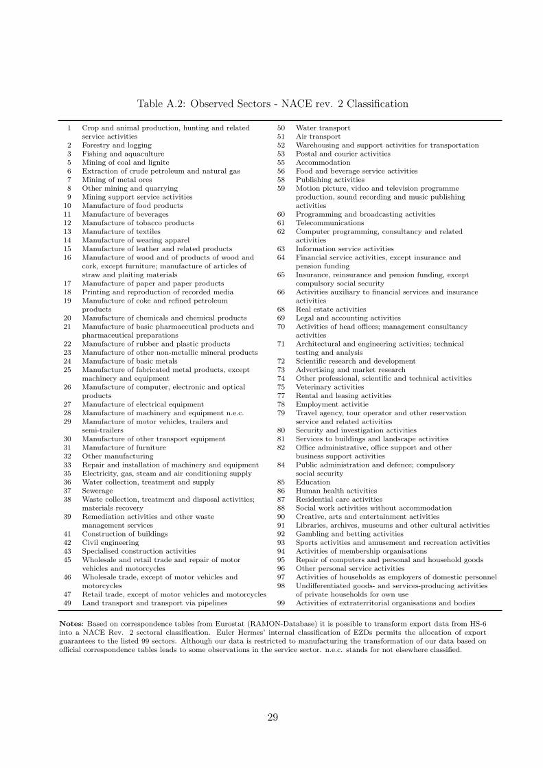
Figure II shows that the share of exports covered by Hermes (EZD only) differs stronglyacross industries (classified according to NACE rev. 2).15 The highest coverage ratios arefound in the aircraft industry (10%) followed by the machinery sector (6%). Other indus-
13In 2009, the World Bank reports a drop in global trade by 22% and in Germany by 18.4%. Eaton et al.(2011) and Yi (2009) argue that the major reason for that strong decline was a disproportionately strongdrop in demand for traded goods. Chor and Manova (2011) among others additionally claim that constraintsin trade finance played a crucial role during the recent economic collapse.
14Appendix A.1 lists the countries in each risk category.15Only industries with positive Hermes EZD coverage are shown. Euler-Hermes does not report the
distribution across industries of insurance instruments other than EZD.
5
Figure I: Export and Hermes Guarantee Shares Across OECD-Risk Groups
Notes: Export shares are calculated based on UN-COMTRADE data (BACI database with corrected trade flows). Exportdestination countries are categorized according to OECD Country Risk Classification. Countries with the lowest risk areclassified as 0 (e.g. France), very risky ones as 7 (e.g Afghanistan). Hermes Guarantee volumes are provided by Euler-Hermes.Stacked bars in the left panel depict yearly German export distributions (1=100%) across three different groups categorizedalong the OECD risk classification. Accordingly, in each considered year German exports are predominantly sold to low riskdestinations. Stacked bars in the right panel illustrate that a major share of German export credit guarantees are claimed forexport destinations with a risk class larger than 1. Six percent of German trade goes to unclassified countries.
tries with high coverage are electrical equipment (3%) and railway locomotives (2%). Theseindustries are characterized by long-term and large export deals. By contrast, the leadingtwo export industries (motor vehicles and chemicals) which feature short-term and relativelysmaller transactions exhibit a coverage of foreign sales with EZD below 1%. These patternsshow that next to country-specific features (policy or business conditions), industry-specificaspects (size and duration of projects) appear to play a crucial role for the use of Hermesguarantees.
At times in the past, the issuance of public export credit insurance had led to substantiallosses for the German tax payer. Accumulated losses from export credit claims amounted to13.4 billion Euro in 1999, mostly because of losses related to the Russian financial crises of1998. Since 2006, however, the cumulative effect of Euler-Hermes guarantees on the federalbudget has been positive and stands at 2.6 billion Euro at the end of 2011. Nonetheless, givenan exposure of almost 30 billion Euro per year, it is of obvious public and political interestto know whether those guarantees have indeed stimulated economic activity by increasingsales, employment, and value added relative to the hypothetical counterfactual of no publicinsurance. In this paper, we carry out such an analysis at the firm level. While our strategy
6
Figure II: Export Volumes and Hermes Coverage by Sectors in 2009
124.86
121.45
119.02
53.77
41.72
28.91
22.33
18.42
13.83
9.68
3.79
3.76
2.23
0.16
0 50 100 150Exports in Billion Euros
Motor Vehicles & Trailers
Chemicals & Chemical Prod.
Machinery & Equipment
Computer, Electronic & Optical Prod.
Basic Metals
Electrical Equipment
Fabricated Metal Products
Air & Spacecrafts
Medical & Dental Instruments
Electric Motors, Generators, Transformers
Machinery for Mining, Quarrying
Railway Locomotives
Ships & Boats
Other Transport Equipment
Export Volume by Sectors
0.11
0.00
5.62
0.62
0.04
2.98
0.35
9.53
0.62
0.55
0.01
1.80
0.50
0.24
0 2 4 6 8 10Hermes Guarantees/Exports −− in %
Hermes Coverage by Sectors
®Notes: Sector classification is in NACE rev. 2. Sectoral export volumes are derivedfrom HS-6 BACI data by using correspondence tables from the RAMON databaseand Eurostat. Export credit guarantees include Einzeldeckungen (EZD), which canbe assigned to specific sectors. Appendix A.2 list the sectoral nomenclature. Sectorswithout Hermes guarantees are excluded. Source: Euler-Hermes and BACI database.
precludes general equilibrium and welfare considerations, it is the first to explore the causaleffect of guarantees using firm-level data. In the next section we first present descriptivestatistics about firms with and without Hermes guarantees treatment, before moving on toexplaining our empirical strategy.
3 Firm-Level Data
Euler-Hermes has provided us with 4850 names and addresses of all German firms thatreceived Hermes guarantees between 2000 to 2010. These firms are predominantly manu-facturers. We merge these data with information from the Amadeus database provided byBureau van Dijk Electronic Publishing GmbH (BvDEP).16 The Amadeus data base oversam-ples large firms. However, in the more recent years we are able to identify up to 80% of all
16In Germany, private data, such as those from Euler-Hermes cannot be merged with official firm-leveldata (AfiD-panel) without making the resulting data set public. This was no available option in the presentcontext. To satisfy German data protection regulation, the merge of Euler-Hermes and Amadeus firm datawas carried on by the Economics and Business Data Center at Munich University.
7
“Hermes” firms. The Amadeus data for Germany does not contain information on exports.Therefore, we merge a separate database, DAFNE, also available at Bureau van Dijk E. P.GmbH. Merging Amadeus and DAFNE leads to some loss of observations. Moreover, theexport variable in DAFNE is problematic, since it is not surveyed at a yearly basis. Weuse the available cross-section to identify firms as exporters and restrict our sample to thosefirms. Patchy time-coverage of the export share variable makes it impossible to use exportsas a dependent variable in our analysis.
After eliminating duplicates and further inconsistencies, our sample contains 35,852 ob-servations of exporting firms.17 Out of these observations, 7,776 turn out to provide infor-mation about the main variables. Among them, in 1,391 observations we observe Hermestreatment.18
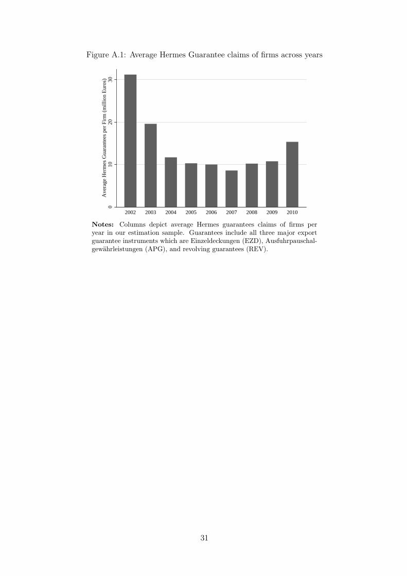
In 2002, the average size of a guarantee extended to a Hermes firm was 30 million Euros.In the succeeding years that average steadily decreased and reached a minimum of eightmillion Euros in 2007, reflecting at the same time a wider use of the instrument as morefirms expanded into markets covered by Hermes and smaller projects. Interestingly, duringthe financial crisis the average provision of Hermes guarantees per firm increased only slightlystaying at around 10 million Euros but increased significantly in 2010, mostly due to theeasing of the OECD Arrangement between 2009 and 2012 as explained earlier. Figure A.1in the Appendix contains details.
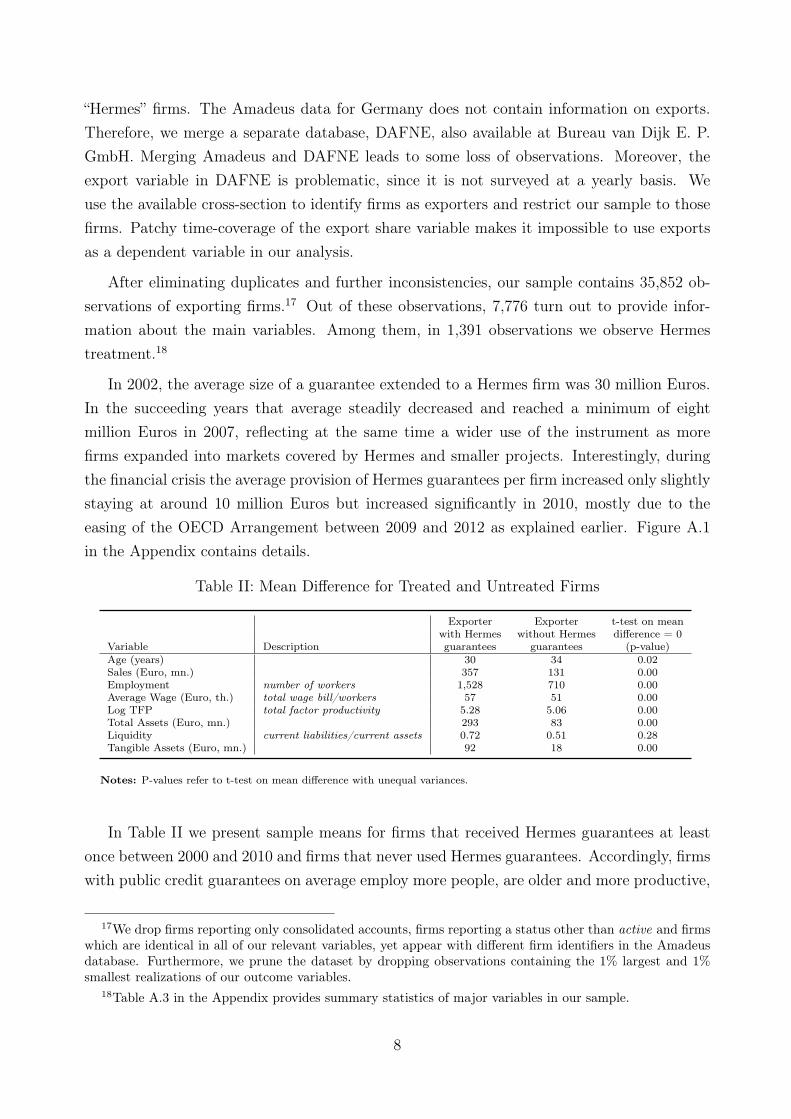
Table II: Mean Difference for Treated and Untreated Firms
Exporter Exporter t-test on meanwith Hermes without Hermes difference = 0
Notes: P-values refer to t-test on mean difference with unequal variances.
In Table II we present sample means for firms that received Hermes guarantees at leastonce between 2000 and 2010 and firms that never used Hermes guarantees. Accordingly, firmswith public credit guarantees on average employ more people, are older and more productive,
17We drop firms reporting only consolidated accounts, firms reporting a status other than active and firmswhich are identical in all of our relevant variables, yet appear with different firm identifiers in the Amadeusdatabase. Furthermore, we prune the dataset by dropping observations containing the 1% largest and 1%smallest realizations of our outcome variables.
18Table A.3 in the Appendix provides summary statistics of major variables in our sample.
8
realize higher sales, have more assets, and pay higher wages. Except for the liquidity ratio,all mean differences are significant at least at the 5 percent level. The apparent differencesbetween the group of treated and untreated firms underlines the concern that selection intotreatment is an issue. Fortunately, our data offers a rich set of firm characteristics from whichwe can select variables that we consider to be relevant for selection. We describe this choiceof variables in detail in Section 5. Before, we describe our estimation strategy and how wedeal with unobserved determinants of selection.
4 Empirical Strategy
4.1 Estimating The Treatment Effect of Hermes Guarantees
Let Hi,s,t ∈ (0, 1) be a dummy variable which takes the value one if a firm i in sector sreceived public export guarantees in year t and zero otherwise. We are mostly interested inthe effect of Hi,s,t on an outcome Yi,s,t, such as employment or sales. A natural but probablynaive linear model would be
where the vector Xi,s,t contains control variables, vs,t is an industry-year effect, vi capturesfirm-specific unobserved heterogeneity, and εi,s,t is an error term. The coefficient δ estimatesthe average treatment effect (ATE) of Hermes guarantees on our outcome variables Yi,s,t,i.e., the average difference between the outcome of a treated and an untreated firm thatis associated with the treatment status of a firm. A common strategy to absorb vi is tofirst-difference the equation or to use fixed effects estimation. A fundamental but plainlyproblematic assumption for consistent estimation of δ is random assignment of Hermes guar-antees to exporters conditional on controls.
In the absence of a suitable instrumental variable, we apply matching estimation to gen-erate consistent estimates of the treatment effect δ. The general idea behind the matchingapproach is to construct the counterfactual outcomes by means of clone firms which are iden-tical in every relevant respect except the treatment status. The method has been widelyapplied in the policy evaluation context, mostly on labor market programs (LaLonde (1986),Gobillon et al. (2012), to mention only very few examples,) but also on the trade effects offree trade agreements (Egger et al., 2008), or currency unions (Baldwin and Taglioni, 2007).19
Besides dealing with endogenous selection into treatment, matching estimation does not relyon a functional form assumption regarding the relationship between observable characteristics
19Blundell and Dias (2009) and Imbens and Wooldridge (2009) provide an overview over methods.
9
and the outcome variable and it avoids predictions into ranges of observables that are out-side the support of the group of treated units. Moreover, linear models estimate the averagetreatment effect (ATE), which, in the presence of endogenous selection into treatment, differsfrom the average treatment effect on the treated (ATT).20 In the context of policy evaluation,however, the ATT is of larger interest as it reflects the effects of Hermes guarantees on thosefirms, that have actually taken part in the program.
Let Y 0i and Y 1
i denote the potential outcomes for firm i depending on its treatment statusHi ∈ (0, 1). Then, the ATE is given by ATE = E(Y 1
i − Y 0i ), where E is the expectation
operator. The ATT is obtained from a comparison of potential outcomes only for firms thatare indeed treated, i.e. it is given by ATT = E(Y 1
i − Y 0i |Hi = 1). The ATT differs from the
ATE if the difference in potential outcomes depends on firm characteristics and the averagetreated firm differs from the average untreated firm with respect to these characteristics.Identification and consistent estimation relies on three assumptions. The first one is theconditional independence assumption (“selection on observables”, (Rosenbaum and Rubin,1983)):
(Y 0i , Y
1i ) ⊥ Hi|Xi, (2)
where⊥ denotes independence. It states that conditional on a set of observable characteristicsXi, the potential outcome for each firm is independent of the treatment status. Hence, underthe conditional independence assumption the counterfactual outcome for any firm is identicalto the outcome of its control firm which exhibits identical observable characteristics butthe opposite treatment status, and therefore, any difference in outcomes between a pair ofmatched firms can, in expectations, be attributed to the treatment. The second assumptionis the overlap assumption, which requires that firm characteristics Xi do not perfectly predictthe treatment status. In other words, for each combination of firm characteristics there mustpotentially exist both firms with and without treatment.21 The third requirement is thestable unit treatment value assumption (SUTVA), which states that the impact of Hermesguarantees on one firm is independent of the allocation of treatment among the other firms.
Under these assumptions, a consistent estimate of the sample average treatment effect
20The ATE can be interpreted as the expected value of the treatment effect for a firm that has the averagecharacteristics of the sample. In contrast, the ATT reflects the expected value of the treatment effect for afirm that has the average characteristics of the subsample of treated firms.
21If the conditional independence and the overlap condition simultaneously hold Rosenbaum and Rubin(1983) refer to this as “strong ignorability”.
10
(SATE) is given by
SATE =1
N
N∑i=1
(Y 1i − Y 0
i ) (3)
where Y 1i = Yi if Hi = 1 and Y 1
i =(∑k
j=1 Yij
)/k else; and Y 0
i =(∑k
j=1 Yij
)/k if Hi = 1
and Y 0i = Yi else.22 N denotes the sample size, k equals the number of control firms used
in the construction of the counterfactual outcome for firm i and Yij ∀ j = 1, ..., k are theoutcomes of the k control observations for firm i.
Accordingly, the sample average treatment effect on the treated is consistently estimatedas
SATT =1
N1
N∑i=1|Hi=1
(Yi − Y 0i ) (4)
where Yi is the observed outcome of the treated firms, Y 0i = 1
k
∑kj=1 Yij the average outcome
of the control observations for firm i and N1 denotes the number of treated firms in thesample. The choice of appropriate control firms is based on a metric that summarizes thedistance of two firms in the multidimensional space of firm characteristics. Following Abadieand Imbens (2011), we use the Mahalanobis distance metric. We present results based onpropensity scores in our robustness checks.23
The estimation routine proposed by Abadie et al. (2004) allows to specify variables onwhich matching is performed exactly, hence, it enables us to match firms within narrowlydefined sector-year cells without estimating a huge set of parameters in a first step. TheMahalanobis distance mij(xi, xj) between two firms i and j with opposite treatment status iscalculated as mij(xi, xj) =
√(xi − xj)TS−1(xi − xj), with S representing the sample covari-
ance matrix or a diagonal matrix of sample variances of X. Hence, the Mahalanobis metricis based on the Euclidean distance ‖ xi−xj ‖ in matching variables X between firms i and j.In a one-to-one match (k = 1), the firm j that is closest to firm i in terms of mij is chosen ascontrol observation and receives a weight one. Besides one-to-one matching, the method alsopermits k-nearest neighbor matching, in which the k nearest neighbors are chosen as controls
22Note that the estimator for the sample average treatment effect is identical to the estimator of thepopulation average treatment effect. Differences arise in the estimation of the variance (cf. Abadie andImbens, 2011).
23The propensity score, i.e. the predicted probability of obtaining treatment given observed covariatesP (Hi = 1|Xi), is usually obtained from a first stage Probit or Logit estimation. Since we want to control forsector and time specific unobserved heterogeneity, conditional Logit with fixed effects would be the optimalchoice for our case. However, given the relatively small number of treated firms in our sample and the largenumber of parameters to be estimated in the first stage, we prefer the Mahalanobis metric as distance measurefor the matching.
11
entering with weights wij = 1/k. In our empirical evaluation, we let k vary from 1 to 5.
Abadie and Imbens (2006) show that estimates of the treatment effects from finite samplessuffer from a bias due to remaining differences in covariates, with the severity of the biasincreasing in the number of continuous covariates. Abadie and Imbens (2011) propose a bias-correction for the estimators that accounts for differences in covariates within the matches,by correcting for differences in predicted outcomes obtained from ordinary least squares. Thebias-corrected estimator replaces Y 0
i in (4) by
Y 0i =
1
k
k∑j=1
(Yij + µ0(Xi)− µ0(Xij)) , (5)
where µ0 is the predicted outcome of the linear model µ0(X) = β00 + β01X.24 We use thisbias adjustment in all of our baseline specifications.
4.2 DiD-Matching
To relax the selection on observables assumption one can use matching in differences (DiD-matching). Comparing changes in the outcome variables of the group of treated firms tochanges in the outcome of the control group allows to neglect time-constant unobservedfactors that simultaneously affect the treatment status and the level of the outcome variables.Assuming that the treatment occurred between period t and t− 1, the SATT based on DiD-matching can be estimated by comparing changes in the outcome variable of treated firmsbetween t−1 and t with the respective changes in the outcome variable in the control group:
SATTDID,bc
=1
N1
N∑i=1|Hi=1
((Y 1
i,t − Y 1i,t−1)− (Y 0
i,t − Y 0i,t−1)
), (6)
where Y 0i,t and Y 0
i,t−1 are defined in (5).
A sharp definition of the pre-treatment period, which is necessary to consistently deter-mine the changes in the outcome variables, implies that we can only use those treatmentobservations where we observe changes in the treatment status to identify the treatment ef-fect. We therefore define the treatment dummy to Hermes which equals one in period t ifthe firm changes from no treatment in t − 1 to treatment in period t and zero otherwise.25
24Coefficients are estimated by weighted least squares (WLS) based on the subsample of control obser-vations weighted by the number of times they are used as control firms (for details see Abadie and Imbens,2011).
25Alternatively, we could also use the exit from treatment to identify the effect. However, the highlikelihood that treatment occurs in lagged periods prevents us from doing so.
12
While DiD-matching reduces the number of treatment observations, it strongly enhances ourconfidence in the reliability of our results.
Finally, when matching is based on pre-treatment variables, differences in time trends inthe covariates across the groups of treated and control firms can lead to biased estimates.Heckman et al. (1997) propose a regression-adjusted matching estimator that controls fordifferent time trends in observable covariates. The regression-adjusted estimator for theSATT is then
SATTDID,ra
=1
N1
N∑i=1|Hi=1
((Y 1
i,t − Y 1i,t−1)− (Y 0
i,t − Y 0i,t−1)
)(7)
where Y 1i,t = Y 1
i,t − Xi,tβ0 and Y 0i,t = 1
k
∑kj=1
(Y 0ij −Xij,tβ0
). Instead of the conditional
independence assumption this estimator requires that the distributions of unobservable char-acteristics be equal across treated and untreated firms (Heckman et al., 1998).26 Regression-adjusted matching allows us to check the robustness of our results from the preferred speci-fication with respect to the common time trend assumption.
4.3 Identification Strategy
We define a firm as treated in t if it experienced a change in its Hermes status from noguarantee in t − 1 to a guarantee in t and compare the average change in the outcomevariable in the group of firms treated in that way to the average change in the controlgroup. Control firms are selected based on average pre-treatment values of appropriatelychosen control variables; see the discussion below. We take account of the bias arising fromdifferences in covariates as described by Abadie and Imbens (2006) by applying the bias-correction in (5) to our DiD-estimator in our baseline specification. To take account of thepotential bias arising from different time trends in covariates we also estimate the treatmenteffect using regression-adjusted matching as described in (7). Besides removing time-constantfirm specific unobserved heterogeneity through differencing, we also control for sector-timespecific influences by matching within sector-year cells. In our baseline estimation, sectorsare defined on the 2-digit level of the NACE rev. 2 classification.27
To assess the validity of the conditional independence assumption, we test for the balanc-ing property and estimate pseudo treatment effects. The latter allows to assess whether our
26This procedure is analogous to a difference-in-difference estimation along the weighted linear regressionspecification in equation (1) estimated in changes. Weights are derived from the nearest neighbor matchingbased on the Mahalonobis distance metric calculated from pre-treatment values of the covariates X.
27Naturally, a stronger disaggregation of sectors comes at the cost of a smaller pool of potential controlfirms. In our robustness analysis we test the sensitivity of our results with regard to this choice.
13
groups of treated and control firms exhibited significantly different changes in the outcomevariables in any periods other than the period of treatment.
Altogether, we find very robust evidence for a positive effect of Hermes guarantees onfirms’ sales and employment and we are confident that our approach identifies causal effects.Before we present the results in detail in Section 6, we first discuss our choice of matchingvariables and the common support assumption in the following section.
5 Matching Variables and Common Support
5.1 Matching Variables
Our strategy requires that all variables which influence the change in the treatment statusand in the outcome variables are accounted for in the matching process. Although the choiceof variables is crucial, the econometric literature provides little guidance on how to choosecovariates. So, we use relevant economic theory and related empirical work to guide ourchoice of matching variables. According to recent heterogeneous firms theory (based onMelitz, 2003), the share of exports in total sales is higher in firms that are more productive,larger, and older, and have relatively more skilled employees compared to only domesticallyactive firms.28 Hence, a first set of matching variables include measures of total factorproductivity (TFP), size, age and a measure of skill intensity of production.29 We use totalassets, tangible assets, employment, and sales to capture firm size and total wage bill overnumber of employees to approximate skill intensity, (see also Wagner, 2011). A second set ofvariables is motivated by recent trade literature focusing on the role of trade credit frictions.Chor and Manova (2011) illustrate that sectors with higher external financial dependenceexperienced a stronger reduction in foreign sales. Following Chor and Manova (2011) andothers, we construct two indicators that measure firms’ access to external finance. The firstone is the stock of tangible assets, where we expect that a higher stock of tangible assetsmitigates credit constraints as tangible assets can serve as collateral. The second measureis liquidity measured as current liabilities over current assets. A smaller liquidity ratio thenindicates better access to external finance.
This constitutes our set of firm characteristics. We match on pre-treatment averagesof the firm variables as all of them (except age) are more or less likely endogenous to thetreatment itself. Furthermore, we add pre-treatment averages of sales growth. This choice of
28A large strand of empirical literature provides solid evidence for these theoretical results (see e.g. Bernardand Jensen, 1999, 2004; Wagner, 2007; Bernard and Wagner, 2001).
29TFP is estimated using the methodology developed by Olley and Pakes (1996).
14
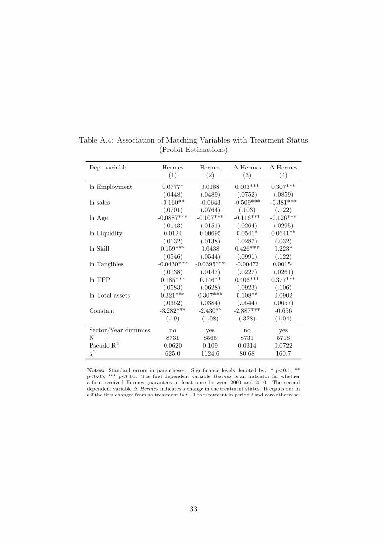
matching variables confines us to a sample of firms that report sufficiently detailed data andare observed for at least two consecutive years. Since data availability is strongly correlatedwith the size of firms, our estimation sample is not representative for the subpopulationof firms in the Amadeus database. However, since our concern is an ex-post evaluation ofexport credit guarantees by means of the sample average treatment effect on the treated, thisdoes not constitute an obstacle to our analysis. We assess the association of the matchingvariables with the treatment status by means of probit estimations and pairwise correlations.Results are collected in Table A.4 and Table A.5 in the Appendix. Both exercises show thatour matching variables and the treatment status are strongly correlated.
5.2 Assessing Common Support and the Balancing Property
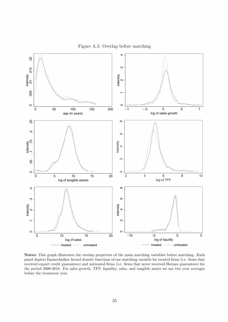
As described above, identification of treatment effects relies on the validity of the commonsupport or overlap assumption. For each set of firm characteristics, we must potentially beable to observe treated and untreated firms. Ideally, the assessment of the validity of theoverlap assumption would be based on the multivariate distribution of the matching vari-ables. Since this is not feasible, we compare the marginal distribution of each covariate forHermes and non-Hermes firms. Figure A.3 in the Appendix presents kernel densities for ourfinal choice of variables before matching. We find substantial overlap for all matching vari-ables.30 Furthermore, we drop firms in sector-year cells in which no treated or no untreatedfirms are present to ensure overlap in our exact matching variables. As expected from ourdiscussion of selection into treatment, for the pre-matching samples the estimated densitiesdiffer significantly between the groups of treated and untreated firms.
We assess the balancing property by comparing mean difference tests for the pre- andpost-treatment samples. As illustrated in the upper part of Table III, the null hypothesisof identical means between treated and untreated firms (t-test) is rejected for all relevantvariables in the pre-matching sample. Equally, the Kolmogorov-Smirnov test rejects equalityof the respective distributions. The lower part of Table III shows the same statistical testsfor the relevant variables after our preferred Mahalanobis nearest neighbor matching (withone nearest neighbor). In the matched sample, differences have decreased significantly. Ac-cordingly, the null hypothesis of identical means between treated and untreated firms can nolonger be rejected and the Kolmogorov-Smirnov test does not reject equality of the respec-tive distributions (except for average total assets). We treat these results as support thatour matched sample fulfills the balancing property.31
30We minimally trim our sample by dropping the largest 0.01% of observations of all relevant matchingvariables.
31We find qualitatively similar results for the samples obtained from matching k>1 nearest neighbors.
15
Table III: Differences between Treated and Untreated Firms Before and After Matching
Kolmogorov-Smirnov-Test (p-values)H0: Equality of H1: Difference H2:Difference
Variable Enterprises Enterprises t-test on Distribution in favor for in favor for(Two-year with Hermes without Hermes Mean Difference btw treated and untreated treatedaverage) guarantees guarantees (t-statistics) untreated firms firms firms
Notes: Compared variables are two year averages before treatment occurs. The matching sample is obtained from matchingk=1 nearest neighbors with ∆ ln Sales as outcome variable. Similar results hold for higher k and ∆ ln Employment as outcomevariable. The t-test on mean difference assumes unequal variances for both groups of firms. Regarding the Kolmogorov-Smirnovtest, H0 test for equality of the respective distributions, H1 tests whether the distribution of firm characteristics of untreatedfirms stochastically dominates those of the Hermes firms and H2 test the opposite hypothesis. Sales, Skill (Wage bill/workers),Total assets, Tangibles are in thousand Euro. Liquidity is defined as current liablities/current assets.
6 Evaluating Public Export Credit Guarantee Effects
6.1 Results from DID-Matching
Table IV shows the estimated treatment effects on sales and employment from the differentmatching strategies discussed in Section 4. We estimate four different specifications (whichare found in columns one to four) and use different numbers of nearest neighbors in theconstruction of the counterfactuals (reported in rows one to five).
Column (1) in Table IV contain the treatment effects estimates on sales and employment,respectively, obtained from the bias-corrected DiD-estimator as specified in (6). This consti-tutes our preferred specification. The estimates show that export credit guarantees triggersales growth of 3.9 to 4.8 percentage points and employment growth of 2.5 to 3 percentagepoints, respectively. Comparing the coefficient estimates to those in column (2), where wepresent the uncorrected matching estimates, shows that the bias correction primarily makes a
16
Table IV: Baseline Results: Sample Average Treatment Effects on the Treated (SATT)
Notes: Treatment effects are estimated as changes in log outcomes in the year of the treatment,where treatment in t is defined as the change in treatment status from no treatment in t− 1 totreatment in t. Matching variables are pre-treatment two-year averages of TFP, skill, tangibleassets, liquidity, employment, sales, sales growth, age, and total assets. Matching is performedwithin sector-year cells, where sectors are defined on 2-digit level of NACE rev. 2. ∗,∗∗ ,∗∗∗
indicate significance on the 10,5, and 1% significance level, respectively. a) N and N treatedrefers to the number of firms entering the matching process in the first stage. The number offirms entering the second stage depends on the number of nearest neighbors used in the firststage and on the availability of data on contemporaneous changes in the covariates. The numberof treated (untreated) firms in the second stage from the estimation with k = 1, 2, 3, 4, 5 nearestneighbors equals 35,45,53,56,59 (35,61,94,120,149) for sales and 32,50,52,55,59 (32,67,99,126,159)for employment.
difference for sales, where coefficients from the uncorrected estimation turn out to be slightlysmaller. Employment effects are hardly affected. Column (3) presents the treatment effectestimates obtained from the regression-adjusted matching estimator described in (7). Salesand employment effects turn out positive and significant. The coefficients are larger bothin the case of sales and employment, in particular for small numbers of nearest neighbors.This could indicate that differences in the time trends of the covariates matter. However,
17
it must also be taken into account that we lose a significant number of observations as theregression-adjusted matching estimator requires information on contemporaneous changes inthe control variables which are not available for all firms in our quasi-experimental dataset.As the number of nearest neighbors increases, the coefficient estimates come much closerto those obtained from our preferred specification. Additionally, in column (4) we presentresults from propensity score matching, which, in the case of employment confirm the resultfrom the Mahalanobis matching. In the case of sales we find significant treatment effectsonly for k < 3 nearest neighbors.
Summarizing, we find that, throughout our different specifications , Hermes guaranteeshave positive effects on sales and employment, which are statistically and economically sig-nificant. In our sample, treatment leads to an average increase in sales growth by about 3.9to 4.8 and in employment growth by 2.5 to 3 percentage points, respectively, in the year aHermes Guarantee is granted. Considering that the treated firms in our sample cover onaverage 6.6 percent of their sales by a guarantee, the magnitudes are plausible. The effectsare also economically significant; we find that the average increase in sales induced by thegrant of a guarantee amounts to 4.25 million Euro, corresponding to an average guaranteevolume of 6.04 million Euro. Employment increases by 55 employees on average.32
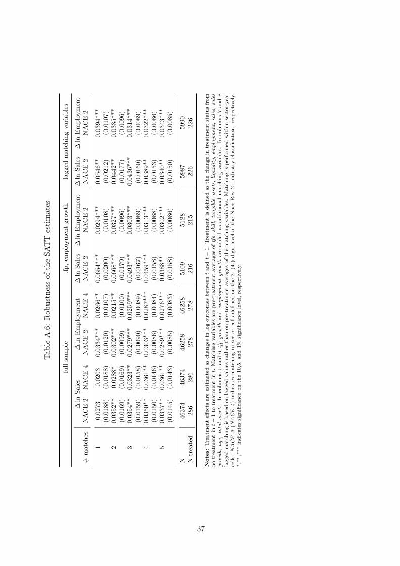
Based on these results, we further check the robustness of our estimations with respectto a larger sample, a different level of sectoral disaggregation and the choice of matchingvariables. Table A.6 in the Appendix summarizes the results of the additional specifications.We perform the same matching procedure in a sample of 47,000 firms to increase the numberof potential controls. Unfortunately, we lack information on exporting status of these firms.However, since the other matching variables, in particular, TFP, size measures, and the proxyfor skill intensity, all correlate strongly with export status, we believe that this robustnesscheck is sensible. We find that the results are robust in terms of significance and in termsof size to the sample composition (cp. columns (1) and (3)). Only for the case of firm salesperformance do the effects turn out to be slightly smaller, dropping to a range of 3.5 to 4percentage points and are insignificant for k = 1. We repeat the exercise now defining sectorcells more restrictively on the 4-digit level of the NACE rev. 2 industry classification, whichis feasible in the larger sample. The results presented in columns (2) and (4) are hardlyaffected.
Next, based on the original sample, we choose a larger set of matching variables byincluding pre-treatment averages of employment growth and TFP growth as they mightpotentially affect the selection into Hermes. The larger number of matching variables comesat the cost of a lower number of observations in both the group of treated and potential
32To quantify the effects, we use a sales (employment) weighted average of the estimated individualtreatment effects obtained from matching with five nearest neighbors.
18
control firms. However, we find that results are not affected in terms of significance and interms of size for larger number of nearest neighbors (cp. columns (5) and (6)). Using laggedvalues of the treatment variables instead of pre-treatment averages also does not change theresults by much (columns (7) and (8)).
6.2 Treatment Effects on Additional Outcome Variables
In Table V we present estimated treatment effects of Hermes guarantees on different outcomevariables, namely value added, value added per worker, the average wage (firm level wage billdivided by number of workers), and profits over sales (the EBIT/sales ratio). Except for thelatter, all variables are in logs. Compared to sales or employment, these outcome variablesare more problematic because they are constructed from balance-sheet positions reportedby firms. In particular, value added poses problems since it can turn negative. By takinglogs, these observations drop out so that the sample differs from the one used to computetreatment effects on sales or employment.
For all outcome variables and regardless of the number of nearest neighbors (k), weestimate positive treatment effects that are at maximum 6 percent. We find that treatmentincreases growth of value added by between 4.4 and 6.1 percentage points, while the growthof value added per worker goes up by between 2.7 and 3.0 percentage points.33 These resultssuggest that Hermes guarantees boost value added by more than employment, the relativeimportance of employment being about a third. We further decompose value added into awage and a profit component and find that the change in average wages increased by about1.5 percentage points. We also find marginally significant positive effects on the profit salesratio.
6.3 Assessment of the Conditional Independence Assumption
We assess the validity of the conditional independence assumption by means of pseudo treat-ments, i.e. we compute treatment effects on our variables in years where no treatment tookplace. As Imbens and Wooldridge (2009) point out, pseudo treatments cannot be consid-ered a test of the conditional independence assumption. However, they can be used to ruleout obvious violations of the assumption, such as significant differences in changes in theoutcome variables between the group of treated and controls in periods where no treatmenttook place. The absence of pseudo treatment effects enhances our confidence that the realtreatment effects are causal.
33These results suggest (e.g., for k = 1) that employment should go up by about 2 percent. This is almostexactly what we find in Table IV.
19
Table V: Treatment Effects on Additional Outcome Variables
Outcome variable:∆ ln Value added ∆ ln Value added ∆ ln Average wage ∆ EBIT/sales
Notes: Treatment effects are estimated as changes in log outcomes in the year of the treatment, wheretreatment in t is defined as the change in treatment status from no treatment in t − 1 to treatment in t.Matching variables are pre-treatment two-year averages of TFP, skill, tangible assets, liquidity, employment,sales, sales growth, age, and total assets. Matching is performed within sector-year cells, where sectors aredefined on 2-digit level of NACE rev. 2. ∗,∗∗ ,∗∗∗ indicate significance on the 10,5, and 1% significance level,respectively.
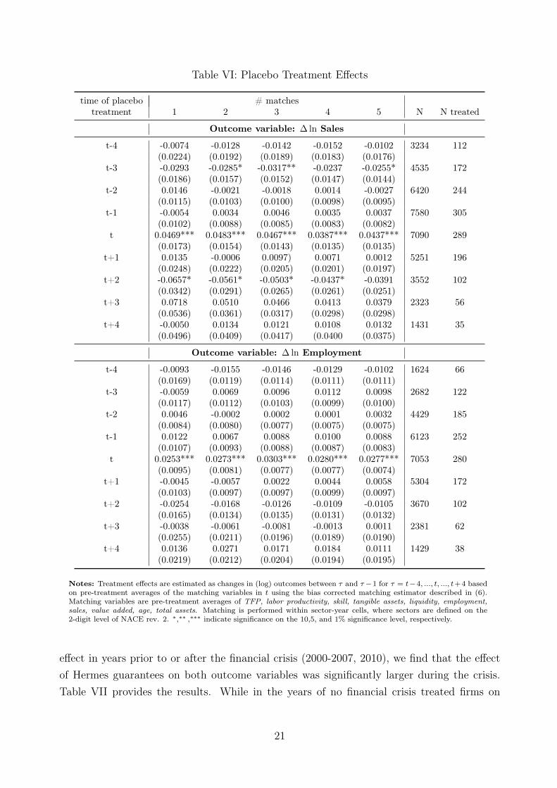
Table VI summarizes such placebo treatment effects on four lags and for future changesof our outcome variables sales and employment. We find that, with few exceptions, there areno significant differences between changes in the outcome variables in our groups of treatedand control firms. Only for sales do we find that firms treated in t experienced a significantlydifferent change in t+2 and in t−3. The estimated differences are negative, weakly significantand not robust across estimations with different numbers of nearest neighbors. Moreover, thefurther we move away from the time of the treatment, the less firms we observe in the groupsof treated and untreated firms and hence, the less representative the estimates become. Int + 2, for example, we observe only 35% of the firms treated in t and about 50% of thepotential control firms. We therefore, do not overemphasize the placebo effect on sales inthose other periods.
6.4 The Effect of Hermes Guarantees in the Financial Crisis 2008/2009
As discussed in Section 2, public export credit guarantees aim at mitigating frictions onfinancial markets that prevent otherwise profitable export business from being realized. Anatural implication of this is that the effect of Hermes guarantees should be particularly strongin times of financial distress, when access to external finance is difficult. An exogenous shocklike the recent financial crisis (2008/2009) offers the possibility to analyze this hypothesis.Comparing the treatment effect of Hermes guarantees during the financial crisis to the average
20
Table VI: Placebo Treatment Effects
time of placebo # matchestreatment 1 2 3 4 5 N N treated
Notes: Treatment effects are estimated as changes in (log) outcomes between τ and τ−1 for τ = t−4, ..., t, ..., t+4 basedon pre-treatment averages of the matching variables in t using the bias corrected matching estimator described in (6).Matching variables are pre-treatment averages of TFP, labor productivity, skill, tangible assets, liquidity, employment,sales, value added, age, total assets. Matching is performed within sector-year cells, where sectors are defined on the2-digit level of NACE rev. 2. ∗,∗∗ ,∗∗∗ indicate significance on the 10,5, and 1% significance level, respectively.
effect in years prior to or after the financial crisis (2000-2007, 2010), we find that the effectof Hermes guarantees on both outcome variables was significantly larger during the crisis.Table VII provides the results. While in the years of no financial crisis treated firms on
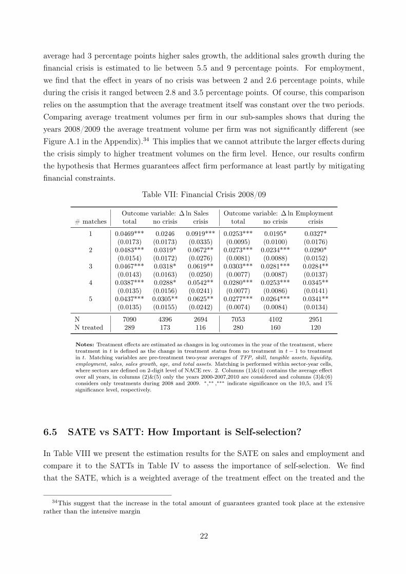
21
average had 3 percentage points higher sales growth, the additional sales growth during thefinancial crisis is estimated to lie between 5.5 and 9 percentage points. For employment,we find that the effect in years of no crisis was between 2 and 2.6 percentage points, whileduring the crisis it ranged between 2.8 and 3.5 percentage points. Of course, this comparisonrelies on the assumption that the average treatment itself was constant over the two periods.Comparing average treatment volumes per firm in our sub-samples shows that during theyears 2008/2009 the average treatment volume per firm was not significantly different (seeFigure A.1 in the Appendix).34 This implies that we cannot attribute the larger effects duringthe crisis simply to higher treatment volumes on the firm level. Hence, our results confirmthe hypothesis that Hermes guarantees affect firm performance at least partly by mitigatingfinancial constraints.
Table VII: Financial Crisis 2008/09
Outcome variable: ∆ ln Sales Outcome variable: ∆ ln Employment# matches total no crisis crisis total no crisis crisis
Notes: Treatment effects are estimated as changes in log outcomes in the year of the treatment, wheretreatment in t is defined as the change in treatment status from no treatment in t − 1 to treatmentin t. Matching variables are pre-treatment two-year averages of TFP, skill, tangible assets, liquidity,employment, sales, sales growth, age, and total assets. Matching is performed within sector-year cells,where sectors are defined on 2-digit level of NACE rev. 2. Columns (1)&(4) contains the average effectover all years, in columns (2)&(5) only the years 2000-2007,2010 are considered and columns (3)&(6)considers only treatments during 2008 and 2009. ∗,∗∗ ,∗∗∗ indicate significance on the 10,5, and 1%significance level, respectively.
6.5 SATE vs SATT: How Important is Self-selection?
In Table VIII we present the estimation results for the SATE on sales and employment andcompare it to the SATTs in Table IV to assess the importance of self-selection. We findthat the SATE, which is a weighted average of the treatment effect on the treated and the
34This suggest that the increase in the total amount of guarantees granted took place at the extensiverather than the intensive margin
22
treatment effect on the untreated, is smaller than the SATT. This implies that the averagetreatment effect on the untreated is smaller than that on the treated, thus providing supportfor the selection hypothesis. While a firm with the average characteristics of the population ofHermes firms experienced additional sales growth of about 4.5 percentage points, a firm withthe average characteristics of our sample would have had additional sales growth of about 3percentage points. The estimated employment effects lie in a similar range. Regarding thelower precision of the ATE estimate, we note that it is based on two estimated counterfactualsrather than one. Besides the counterfactual outcome for the treated group it furthermorerequires estimating the counterfactual for the group of untreated firms. And since the numberof treated firms is small relative to the number of non-treated firms, finding good matches forall untreated firms is significantly harder. The last column of Table VIII presents estimatesof the ATE obtained from linear estimation in first differences. We find fairly similar effects.Hence, there is no evidence that the coefficient estimates obtained from linear models sufferfrom an additional bias due to the assumed linearity or unbalancedness of the sample.
Notes: Treatment effects are estimated as changes in log outcomes in the year of the treatment, where treatmentin t is defined as the change in treatment status from no treatment in t− 1 to treatment in t. Matching variablesare pre-treatment two-year averages of TFP, skill, tangible assets, liquidity, employment, sales, sales growth, age,and total assets. Matching is performed within sector-year cells, where sectors are defined on 2-digit level of NACErev. 2. ∗,∗∗ ,∗∗∗ indicate significance on the 10,5, and 1% significance level, respectively. No. of observations 7, 090and 7, 053, no. of treated 289 and 280 for sales and employment, respectively.
7 Conclusion
Almost all governments in the world offer public export credit guarantees to their exporters.They justify those programs by assuming that private financial markets fail to provide insur-ance for long-term and large-scale export projects to certain markets. This disables potentialexporters to refinance their export business so that projects with positive net present valueremain unrealized. In this paper, we exploit data from the German export credit insurancescheme (Hermes) to test whether firms that have access to publicly guarantees really ex-
23
pand their activity instead of only substituting subsidized insurance for private insuranceor reallocating their sales portfolio to more risky markets. The key challenge is to createa quasi-experimental setup, so that observationally identical firms either have access to theprogram or not.
Earlier empirical work on export credit guarantees used industry-level data and lineargravity-type econometric models. We have the universe of all firms that have obtainedHermes guarantees from 2000 to 2010 and combine these data with the Amadeus data setfor Germany. Rather than studying the effect of Hermes on exports, we look at total salesand employment, thereby focusing on the overall size of firms’ operations. We construct ourquasi-experimental data set using matching methods and conduct a differences-in-differencesanalysis to account for unobserved heterogeneity with respect to firms’ selection into theHermes program.
We find that firms which use Hermes guarantees experience a significant additional in-crease in employment and sales compared to untreated firms. The additional sales growthdue to a provision of a Hermes Guarantee ranges between 4 to 4.5 percentage points in theyear of the grant, additional employment growth of treated firms amounts to about 2.5 to 3percentage points. Our results are robust across a wide range of specifications. Furthermore,we also find that the effect of export credit guarantees was larger during the financial crisis.This supports the hypothesis that credit guarantees work through the mitigation of financialconstraints and help firms to expand the scale of activity.
24
Literature
Abadie, A. (2005). Semiparametric Difference-in-Differences Estimators. The Review ofEconomic Studies, 72(1):1–19.
Abadie, A., Drukker, D., Herr, J. L., and Imbens, G. W. (2004). Implementing MatchingEstimators for Average Treatment Effects in Stata. Stata Journal, 4(3):290–311.
Abadie, A. and Imbens, G. W. (2006). Large Sample Properties of Matching Estimators forAverage Treatment Effects. Econometrica, 74(1):235–267.
Abadie, A. and Imbens, G. W. (2011). Bias-Corrected Matching Estimators for AverageTreatment Effects. Journal of Business & Economic Statistics, 29(1):1–11.
Abraham, F. and Dewit, G. (2000). Export Promotion Via Official Export Insurance. OpenEconomies Review, 11(1):5–26.
Amiti, M. and Weinstein, D. (2009). Exports and Financial Shocks. NBER Working PaperNo. 15556, National Bureau of Economic Research.
Antràs, P. and Foley, C. F. (2011). Poultry in Motion: A Study of International TradeFinance Practices. Working Paper 17091, National Bureau of Economic Research.
Auboin, M. (2007). Boosting Trade Finance in Developing Countries: What Link with theWTO? WTO Discussion Paper No. ERSD-2007-4, Geneva: World Trade Organization.
Baldwin, R. and Taglioni, D. (2007). Trade Effects of the Euro: a Comparison of Estimators.Journal of Economic Integration, 22(4):780–818.
Banerjee, A. V. and Duflo, E. (2012). Do Firms Want to Borrow More? Testing CreditConstraints Using a Directed Lending Program. unpublished manuscript, MIT.
Bernard, A. and Jensen, J. (1999). Exceptional Exporter Performance: Cause, Effect, orBoth? Journal of International Economics, 47(1):1–25.
Bernard, A. and Jensen, J. (2004). Why Some Firms Export. Review of Economics andStatistics, 86(2):561–569.
Bernard, A. B. and Wagner, J. (2001). Export Entry and Exit by German Firms. Review ofWorld Economics (Weltwirtschaftliches Archiv), 137(1):105–123.
Berne Union (2010). Export Credit Insurance Report 2010. Exporta: London No. 4.
Berne Union (2012). Berne Union Yearbook 2012. Yearbook.
25
Blundell, R. and Dias, M. C. (2009). Alternative Approaches to Evaluation in EmpiricalMicroeconomics. Journal of Human Resources, 44(3):565–640.
Chari, A., Chen, W., and Dominguez, K. M. (2009). Foreign Ownership and Firm Perfor-mance: Emerging-market Acquisitions in the United States. NBER Working Paper No.14786.
Chor, D. and Manova, K. (2011). Off the Cliff and Back? Credit Conditions and Inter-national Trade during the Global Financial Crisis. Journal of International Economics,Forthcoming.
Dewit, G. (2001). Intervention in Risky Export Markets: Insurance, Strategic Action or Aid?European Journal of Political Economy, 17(3):575–592.
Eaton, J., Kortum, S., Neiman, B., and Romalis, J. (2011). Trade and the Global Recession.NBER Working Paper No. 16666.
Egger, H., Egger, P., and Greenaway, D. (2008). The Trade Structure Effects of EndogenousRegional Trade Agreements. Journal of International Economics, 74(2):278–298.
Egger, P. and Url, T. (2006). Public Export Credit Guarantees and Foreign Trade Structure:Evidence from Austria. The World Economy, 29:399–414.
Felbermayr, G. and Yalcin, E. (2011). Export Credit Guarantees and Export Performance:An Empirical Analysis for Germany. The World Economy, Forthcoming.
Fisman, R. and Love, I. (2007). Financial Dependence and Growth Revisited. Journal of theEuropean Economic Association, 5(2-3):470–479.
Fleisig, H. and Hill, C. (1984). The benefits and costs of official export credit programs. InBaldwin, R. and Krueger, A., editors, The Structure and Evolution of Recent U.S. TradePolicy, pages 321–358. University of Chicago Press.
Gobillon, L., Magnac, T., and Selod, H. (2012). Do unemployed workers benefit from enter-prise zones? The french experience. Journal of Public Economics, 96(9-10):881–892.
Heckman, J., Ichimura, H., Smith, J., and Todd, P. (1998). Characterizing Selection BiasUsing Experimental Data. Econometrica, 66(5):1017–1098.
Heckman, J. J., Ichimura, H., and Todd, P. E. (1997). Matching as an Econometric EvaluationEstimator: Evidence from Evaluating a Job Training Programme. The Review of EconomicStudies, 64(4):605–654.
Imbens, G. W. (2004). Nonparametric Estimation of Average Treatment Effects under Exo-geneity: A Review. The Review of Economics and Statistics, 86(1):4–29.
26
Imbens, G. W. and Wooldridge, J. M. (2009). Recent Developments in the Econometrics ofProgram Evaluation. Journal of Economic Literature, 47(1):5–86.
Janda, K., Michalíková, E., and Skuhrovec, J. (2012). Credit Support for Export: Economet-ric Evidence from the Czech Republic. Working Papers IES 2012/12, Charles UniversityPrague, Faculty of Social Sciences, Institute of Economic Studies.
Jean-Pierre, C. and Farole, T. (2009). Market Adjustment or Market Failure? World BankPolicy Research Working Paper No. 2003, Washington: World Bank.
LaLonde, R. (1986). Evaluating the Econometric Evaluations of Training Programs. Ameri-can Economic Review, 76:604–620.
Melitz, M. (2003). The Impact of Trade on Intra-Industry Reallocations and AggregateIndustry Productivity. Econometrica, 71(6):1695–1725.
Moser, C., Nestmann, T., and Wedow, M. (2008). Political Risk and Export Promotion:Evidence from Germany. The World Economy, 31:781–803.
Olley, G. and Pakes, A. (1996). The Dynamics of Productivity in the TelecommunicationsEquipment Industry. Econometrica, 64(6):1263–1297.
Paravisini, D., Rappoport, V., Schnabl, P., and Wolfenzon, D. (2011). Dissecting the Effectof Credit Supply on Trade: Evidence from Matched Credit-Export Data. NBER WorkingPapers 16975, National Bureau of Economic Research, Inc.
Rajan, R. G. and Zingales, L. (1998). Financial Dependence and Growth. American EconomicReview, 88(3):559–86.
Rosenbaum, P. R. and Rubin, D. B. (1983). The Central Role of the Propensity Score inObservational Studies for Causal Effects. Biometrika, 70(1):41–55.
Wagner, J. (2007). Exports and Productivity: A Survey of the Evidence from Firm-levelData. The World Economy, 30(1):60–82.
Wagner, J. (2011). Offshoring and Firm Performance: Self-selection, Effects on Performance,or Both? Review of World Economics, 147(2):217–247.
Yi, K.-M. (2009). The collapse of global trade: The role of vertical specialization. In Baldwin,R. and Evenett, S., editors, The Collapse of Global Trade, Murky Protectionism, and theCrisis: Recommendations for the G20. London: CEPR.
27
A Appendix
Table A.1: Country Risk Classifications of the Participants to the OECD Arrangement
Risk Category Country Name
0Australia, Austria, Belgium, Canada, Cyprus, Czech Republic, Denmark, Finland,France, Germany, Greece, Hungary, Iceland, Ireland, Italy, Japan, Korea, Luxembourg,Malta, Netherlands, New Zealand, Norway, Portugal, Singapore, Slovak Republic, Slove-nia, Spain, Sweden, Switzerland, United Kingdom, United States
1 Chinese Taipei, Hong Kong (China)
2 Bahrain, Botswana, Brunei, Chile, China, Kuwait, Malaysia, Oman, Poland, Qatar,Saudi Arabia, Trinidad and Tobago, United Arab Emirates
3Algeria, Bahamas, Brazil, Costa Rica, Estonia, India, Israel, Lithuania, Mauritius, Mex-ico, Morocco, Namibia, Panama, Peru, Russian Federation, South Africa, Thailand,Tunisia
Afghanistan, Argentina, Belarus, Bolivia, Bosnia and Herzegovina, Burkina Faso, Bu-rundi, Central African Republic, Chad, Congo, Congo (Dem. Rep.), Côte d’Ivoire, Cuba,Ecuador, Equatorial Guinea, Eritrea, Ethiopia, Gambia, Guinea, Guinea-Bissau, Haiti,Iraq, Korea (Dem. Republic, North), Kyrgyzstan, Laos, Lebanon, Liberia, Malawi,Maldives, Mauritania, Moldova, Myanmar, Nepal, Nicaragua, Niger, Pakistan, Rwanda,Serbia, Sierra Leone, Somalia, Sudan, Tajikistan, Togo, Ukraine, Venezuela, Zimbabwe
Not Classified
American Samoa, Andorra, Aruba, Barbados, Bermuda, Bhutan, Cayman Islands, Chan-nel Islands, Comoros, Djibouti, Dominica, Faroe Islands, Fiji, French Polynesia, Green-land, Grenada, Guam, Guyana, Isle of Man, Kiribati, Kosovo, Liechtenstein, Macao,Marshall Islands, Mayotte, Micronesia, Monaco, New Caledonia, Northern Mariana Is-lands, Palau, Puerto Rico, Saint Kitts and Nevis, Saint Lucia, Saint Vincent and theGrenadines, Samoa, San Marino, Sao Tome and Principe, Seychelles, Salomon Islands,Suriname, Timor-Leste, Tonga, U.S. Virgin Islands, Vanuatu, West Bank and Gaza
Notes: Within the OECD Arrangement the country risk classification system uses a scale of eight riskcategories (0-7). Accordingly, the country risk classification of high income OECD countries and otherhigh income Euro-zone countries is category 0. The country risk classifications of all other countries aredetermined through the application of rules which account for the payment experience of the participants,the financial situation and the economic situation. Countries with the highest risk are classified in category7. The listed classifications prevailed during the period between July 3 and October 30, 2009.
1 Crop and animal production, hunting and related 50 Water transportservice activities 51 Air transport
2 Forestry and logging 52 Warehousing and support activities for transportation3 Fishing and aquaculture 53 Postal and courier activities5 Mining of coal and lignite 55 Accommodation6 Extraction of crude petroleum and natural gas 56 Food and beverage service activities7 Mining of metal ores 58 Publishing activities8 Other mining and quarrying 59 Motion picture, video and television programme9 Mining support service activities production, sound recording and music publishing
10 Manufacture of food products activities11 Manufacture of beverages 60 Programming and broadcasting activities12 Manufacture of tobacco products 61 Telecommunications13 Manufacture of textiles 62 Computer programming, consultancy and related14 Manufacture of wearing apparel activities15 Manufacture of leather and related products 63 Information service activities16 Manufacture of wood and of products of wood and 64 Financial service activities, except insurance and
cork, except furniture; manufacture of articles of pension fundingstraw and plaiting materials 65 Insurance, reinsurance and pension funding, except
17 Manufacture of paper and paper products compulsory social security18 Printing and reproduction of recorded media 66 Activities auxiliary to financial services and insurance19 Manufacture of coke and refined petroleum activities
products 68 Real estate activities20 Manufacture of chemicals and chemical products 69 Legal and accounting activities21 Manufacture of basic pharmaceutical products and 70 Activities of head offices; management consultancy
pharmaceutical preparations activities22 Manufacture of rubber and plastic products 71 Architectural and engineering activities; technical23 Manufacture of other non-metallic mineral products testing and analysis24 Manufacture of basic metals 72 Scientific research and development25 Manufacture of fabricated metal products, except 73 Advertising and market research
machinery and equipment 74 Other professional, scientific and technical activities26 Manufacture of computer, electronic and optical 75 Veterinary activities
products 77 Rental and leasing activities27 Manufacture of electrical equipment 78 Employment activitie28 Manufacture of machinery and equipment n.e.c. 79 Travel agency, tour operator and other reservation29 Manufacture of motor vehicles, trailers and service and related activities
semi-trailers 80 Security and investigation activities30 Manufacture of other transport equipment 81 Services to buildings and landscape activities31 Manufacture of furniture 82 Office administrative, office support and other32 Other manufacturing business support activities33 Repair and installation of machinery and equipment 84 Public administration and defence; compulsory35 Electricity, gas, steam and air conditioning supply social security36 Water collection, treatment and supply 85 Education37 Sewerage 86 Human health activities38 Waste collection, treatment and disposal activities; 87 Residential care activities
materials recovery 88 Social work activities without accommodation39 Remediation activities and other waste 90 Creative, arts and entertainment activities
management services 91 Libraries, archives, museums and other cultural activities41 Construction of buildings 92 Gambling and betting activities42 Civil engineering 93 Sports activities and amusement and recreation activities43 Specialised construction activities 94 Activities of membership organisations45 Wholesale and retail trade and repair of motor 95 Repair of computers and personal and household goods
vehicles and motorcycles 96 Other personal service activities46 Wholesale trade, except of motor vehicles and 97 Activities of households as employers of domestic personnel
motorcycles 98 Undifferentiated goods- and services-producing activities47 Retail trade, except of motor vehicles and motorcycles of private households for own use49 Land transport and transport via pipelines 99 Activities of extraterritorial organisations and bodies
Notes: Based on correspondence tables from Eurostat (RAMON-Database) it is possible to transform export data from HS-6into a NACE Rev. 2 sectoral classification. Euler Hermes’ internal classification of EZDs permits the allocation of exportguarantees to the listed 99 sectors. Although our data is restricted to manufacturing the transformation of our data based onofficial correspondence tables leads to some observations in the service sector. n.e.c. stands for not elsewhere classified.
29
TableA.3:Su
mmaryStatistics
ofExp
orterSa
mple
Variable
Description
Obs
Mean
Std.
Dev.
Min
Max
Age
(yrs.)
35141
3432.46
0164
Sales(E
uro,
th.)
30020
196718
2241608
01.50e+
08Employment
num
ber
ofwor
kers
19608
9963124
8961
1370684
Total
assets
(Euro,
th.)
35551
144243
2396518
01.87e+
08Tan
gibles
(Euro,
th.)
tang
ible
asse
ts28559
39689
805709
06.45e+
07Wagebill(E
uro,
th.)
26430
39037
400795
02.43e+
07Average
wage(E
uro,
th.)
wag
ebi
ll/wor
kers
18171
52.76
51.99
.04
4468085
lnTFP
lnof
tota
lfac
tor
prod
uctivi
ty9055
5.14
.80
1.51
10.88
Liqu
idity
curr
entlia
bilit
ies/
curr
entas
sets
34705
.57
11.60
01909368
Current
Assets(E
uro,
th.)
35551
79852
1362905
01.10e+
08Current
Liab
ilities
(Euro,
th.)
34708
40155
764302
07.13e+
07APG
(Euro)
Gua
rant
ees
ofty
pe"A
usfu
hrpa
usch
alge
wäh
rlei
stun
gen"
35551
697991
8980487
-1.38e+07
6.45e+
08REV
(Euro)
Gua
rant
ees
ofty
pe"R
evol
vier
ende
Dec
kung
en"
35551
38998
1260691
01.46e+
08EZD
(Euro)
Gua
rant
ees
ofty
pe"E
inze
ldec
kung
en"
35551
740862
1.91e+
070
1.92e+
09Hermes
Her
mes
Stat
us(0
,1)
35551
.14
.35
01
Year
35551
2006.42
2.32
2000
2010
Not
es:Firm
specificaccoun
ting
data
stem
sfrom
theAmad
eusda
taba
seprovided
byBureauvonDijk
ElectronicPub
lishing
GmbH
.Hermes
inform
ationis
prov
ided
byEuler
Hermes.
30
Figure A.1: Average Hermes Guarantee claims of firms across years
010
2030
Ave
rage
Her
mes
Gua
rant
ees p
er F
irm (m
illio
n Eu
ros)
2002 2003 2004 2005 2006 2007 2008 2009 2010
Notes: Columns depict average Hermes guarantees claims of firms peryear in our estimation sample. Guarantees include all three major exportguarantee instruments which are Einzeldeckungen (EZD), Ausfuhrpauschal-gewährleistungen (APG), and revolving guarantees (REV).
31
Figure A.2: Average Hermes guarantees of firms across sectors - over all years
05
1510
Ave
rage
Exp
ort C
redi
t Gua
rant
ees i
n M
io E
uro
17
810
1113
1415
1617
1819
2021
2223
2425
2627
2829
3031
3233
3538
4142
4345
4647
5258
6264
6870
7172
7374
7782
8896
Industries in NACE Rev. 2
Notes: Columns depict average Hermes guarantees of firms in different industries in our estimationsample. Industry classification is in NACE rev. 2. Guarantees include all three major export guar-antee instruments which are Einzeldeckungen (EZD), Ausfuhrpauschalgewährleistungen (APG), andrevolving guarantees (REV). In contrast to aggregate data, export credit guarantees appear in moresectors compared to figure II, since through our firm level data we can allocate APG and REV to therespective sectors.
32
Table A.4: Association of Matching Variables with Treatment Status(Probit Estimations)
Sector/Year dummies no yes no yesN 8731 8565 8731 5718Pseudo R2 0.0620 0.109 0.0314 0.0722χ2 625.0 1124.6 80.68 160.7
Notes: Standard errors in parentheses. Significance levels denoted by: * p<0.1, **p<0.05, *** p<0.01. The first dependent variable Hermes is an indicator for whethera firm received Hermes guarantees at least once between 2000 and 2010. The seconddependent variable ∆ Hermes indicates a change in the treatment status. It equals one int if the firm changes from no treatment in t−1 to treatment in period t and zero otherwise.
33
TableA.5:Pairw
iseCorrelation
ofMatchingVariables
andTr
eatm
entStatus
lnAge
lnEmployment
lnSa
les
lnLiqu
idity
lnSk
illln
Tan
gibles
lnTFP
lnTotal
assets
Hermes
lnAge
1.0000
lnEmployment
0.2259*
1.0000
lnSa
les
0.2277*
0.8459*
1.0000
lnLiqu
idity
-0.0617*
-0.0769*
-0.0913*
1.0000
lnSk
ill0.0054
-0.0343*
0.2553*
-0.0559*
1.0000
lnTan
gibles
0.2539*
0.7743*
0.7645*
-0.0745*
0.0123
1.0000
lnTFP
-0.1012*
-0.1483*
0.3648*
0.0314*
0.4296*
-0.2204*
1.0000
lnTotal
assets
0.2198*
0.8572*
0.9417*
-0.1096*
0.2525*
0.8080*
0.1681*
1.0000
Hermes
-0.0389*
0.1484*
0.2728*
-0.0203*
0.1258*
0.1500*
0.1313*
0.2589*
1.0000
Not
es:A
*indicatessign
ificanceat
thelevelof
0.01.
Her
mes
(0,1)indicateswhether
thefirm
received
Hermes
guaran
tees
atleaston
cebe
tween2000
and2010.
34
Figure A.3: Overlap before matching
0.0
05.0
1.0
15.0
2kd
ensi
ty
0 50 100 150 200age (in years)
®
01
23
4kd
ensi
ty
−1 −.5 0 .5 1log of sales growth
®
0.0
5.1
.15
.2.2
5kd
ensi
ty
0 5 10 15 20log of tangible assets
®
0.2
.4.6
.8kd
ensi
ty
2 4 6 8 10log of TFP
0.1
.2.3
.4kd
ensi
ty
5 10 15 20log of sales
treated untreated
®
0.2
.4.6
.8kd
ensi
ty
−10 −5 0 5log of liqudity
treated untreated
®
Notes: This graph illustrates the overlap properties of the main matching variables before matching. Eachpanel depicts Epanechnikov kernel density functions of one matching variable for treated firms (i.e. firms thatreceived export credit guarantees) and untreated firms (i.e. firms that never received Hermes guarantees) forthe period 2000-2010. For sales growth, TFP, liquidity, sales, and tangible assets we use two year averagesbefore the treatment year.
35
Overlap before matching
0.1
.2.3
.4kd
ensi
ty
5 10 15 20log of total assets
®
0.1
.2.3
.4kd
ensi
ty
0 5 10 15
log of employment
treated untreated
®
Notes: This graph illustrates the overlap properties of the main matching variables before matching. Eachpanel depicts Epanechnikov kernel density functions of one matching variable for treated firms (i.e. firms thatreceived export credit guarantees) and untreated firms (i.e. firms that never received Hermes guarantees) forthe period 2000-2010. For employment, skill and total assets we use two year averages before the treatmentyear.