Abstract A new approximate method for the determinationof natural frequencies of a cantilever beam in free bendingvibration by a rigid multibody system is proposed. UniformEuler-Bernoulli cantilever beams with and without a lumpedmass at the tips are considered. The modelling method con-sists of two steps. In the first step, the cantilever beam isreplaced by lumped masses interconnected by massless flex-ible beams. In the second step, the massless flexible beamsare replaced by massless rigid beams connected throughrevolute and prismatic joints with corresponding springs inthem. Elastic properties of the massless flexible beams aremodelled by the springs introduced. The method proposedis compared with similar ones in the literature.
Über die Bestimmung der natürlichen Frequenz vonKonsolen bei freien Schwingungen: rigidesMehrkörpersystem
Zusammenfassung Es wird eine neue Methode angezeigt,für die approximative Bestimmung der Kreisfrequenz derelastischen, transversal schwingenden Konsole. Diese Me-thode stützt sich auf die Theorie des Mehrkörpersystems.Es wird eine homogene Konsole betrachtet, mit und ohnekonzentrierte Masse auf ihrer freien Ende. Diese Methodebesteht aus zwei Schritten. In erstem Schritt wird die Tra-verse durch ein System von konzentrierten Massen, die ge-genseitig mit elastischen, leichten Kolben verbunden sind,ersetzt. Im zweiten Schritt werden die elastischen Kolbendurch leichte, steife Kolben ersetzt, die gegenseitig mit ro-tierenden und prismenförmigen Gelenken mit entsprechen-
S. Šalinic (B) · A. NikolicUniversity of Kragujevac, Faculty of Mechanical and CivilEngineering in Kraljevo, Dositejeva 19, 36000 Kraljevo, Serbiae-mail: [email protected]
den Federn verbunden sind. Durch diese Federn werden dieelastischen Merkmale der leichten, flexiblen Kolben model-liert. Diese Methode wurde auch mit verwandten Methodenin der Literatur verglichen.
List of symbolsx, y, z Axes of the inertial coordinate frameF Force [N]M Torque of a couple [Nm]u Deflection [m]L Length [m]E Young’s modulus of elasticity [N/m2]Iz Axial moment of inertia for the principal
axis z [m4]i, j, k Unit vectors of axes x, y, and z, respectivelyu, uP Displacement vectors of points B and P ,
respectivelypi Local vector of the ith massless beamKB , KP Stiffness matrices corresponding to points B
and P
qi Displacement in the ith jointci Stiffness of the spring in the ith jointm Mass of the beam [kg]mi Mass of the particle Mi [kg]mT Lumped mass at the tip of the cantilever
beamn Number of equal partsei Unit vector of the axis of the ith jointT Kinetic energy [J]VMα Velocity of the particle Mα
rMα Position vector of the particle Mα
q Vector of generalized coordinatesq0 Vector of zero values of generalized
coordinatesq, q First and second time derivatives of the
q1 Vector of odd generalized coordinatesq2 Vector of even generalized coordinatesq1, q2 Second time derivatives of the vectors q1
and q2M Mass matrixmij Components of the mass matrix MK, K, K� Stiffness matrices of the system0 Zero matrixI Identity matrixMij Block matrices of the matrix MKij Block matrices of the matrix KK�
ij Block matrices of the matrix K�
TΛ,TΠ, B,˜B Matrices
v Eigenvectorwi The ith root of the transcendental equation
Greek variablesθ SlopeΠ Potential energy of the cantilever beamΠc Potential energy of the system of springs in
the jointsχi , χi Identifiers of the joint typeωi The ith natural frequency [rad/s]ωi The ith non-dimensional natural frequency
Superscripts, SubscriptsT Matrix transposition operation−1 Inverse matrix operationq0 Zero values of generalized coordinates
1 Introduction
Among various methods for analysis of elastic bodies, theones that especially single out are those methods that arebased on the idea to replace the elastic bodies with a suit-able system of rigid bodies. In such a way, the applica-tion of well developed methods and formalisms of dynam-ics of rigid bodies is achieved in the analysis of dynamics ofelastic bodies. Therefore, modelling of planar elastic beamswith the use of rigid-elastic superelements has been done in[1]. Rigid-elastic superelements consist of three rigid bod-ies connected by two revolute joints. The bodies within therigid-elastic superelements are also interconnected by suit-able springs. The rigid-elastic superelements are rigidly con-nected to one another. The applications of this methodologyto the problems of robotics and wind turbines were givenin [2] and [3], respectively. In [4], the spatial flexible bod-ies in wind turbine structures were considered. The flexiblebodies (rotor blades, tower, shafts etc.) are modelled by car-danic joint beam elements. The cardanic joint beam elementrepresents a system of four rigid spatial bodies connected by
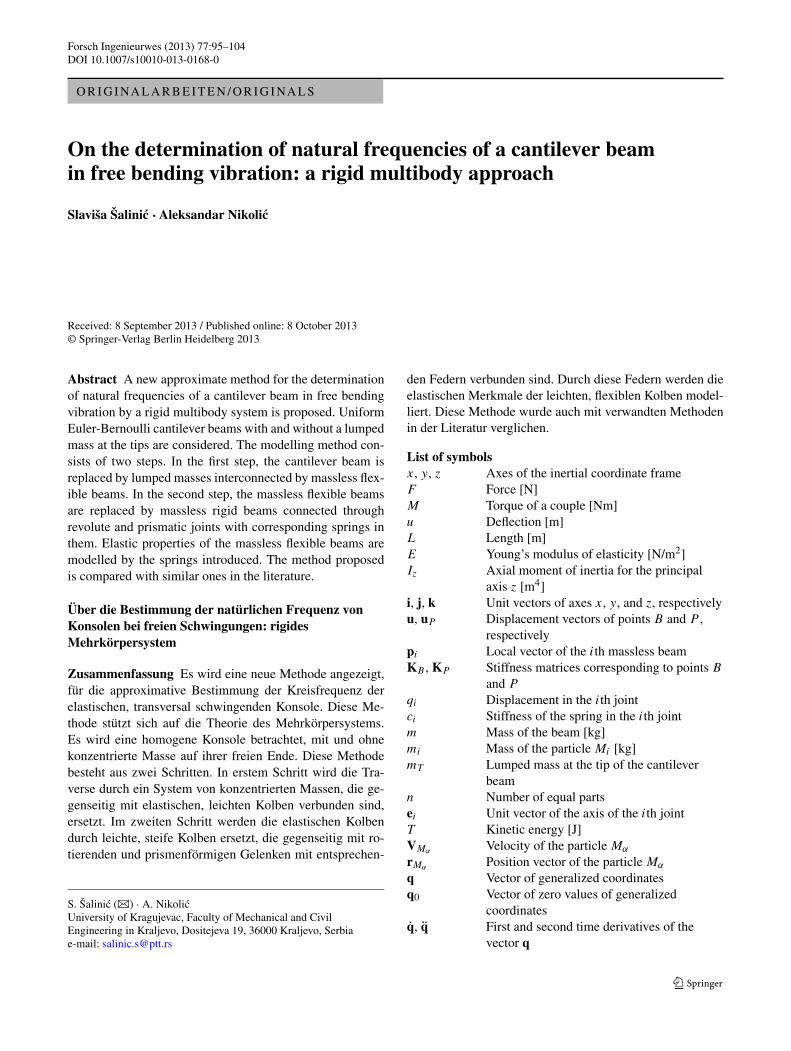
Fig. 1 A cantilever flexible beam with static load
two cardanic joints and one cylindrical joint. In [5], the fi-nite rigid segment method for modelling of flexible beamswas developed. This method consists in that a flexible beamis divided into a finite number of rigid segments connectedwith springs of adequate stiffnesses. The method based onthe similar principles was developed in [6].
In this paper, a method for the analysis of flexible beamsby a system of rigid bodies, as an alternative to the ap-proaches in [1–3, 5, 6], has been proposed. The approachproposed is based on the Routh method of replacing a rigidbeam by an equivalent system of point masses (see [7]). Themethod is illustrated on the problem of the approximativedetermination of natural frequencies of a cantilever beam infree bending vibration. The results are validated against onespublished in the literature.
2 The potential energy of a cantilever flexible beam
In this section, we will derive an alternative expression forthe potential energy of a flexible cantilever beam with staticload at the free end that will be used in further consider-ations. So, let us consider a uniform flexible beam havingclamped end A and free end B (see Fig. 1). The beam istreated as a uniform Euler-Bernoulli beam [9].
Under a static load [F,M]T at the end B , where F is theforce and M is the torque of a couple, the deflection u andthe slope θ are determined by the following relation of thelinear elasticity theory (see for example [1]):
[F
M
]= EIz
L3
[12 −6L
−6L 4L2
][u
θ
]≡ KB
[u
θ
](1)
where the superscript T denotes matrix transposition, KB
is the stiffness matrix of the beam calculated for the endB , L is the length of the beam, E is the Young’s modulusof elasticity, and Iz is the axial moment of inertia for theprincipal axis z of the cross section of the beam. Due tosmall elastic deformations of the beam, the quantities u andθ are small. Let us introduce the following vectors:
u = uj,−→θ = θk, (2)
where i, j, and k are unit vectors of axes x, y, and z, respec-tively. Following the approach from [8], let us imagine now
Forsch Ingenieurwes (2013) 77:95–104 97
that a rigid planar massless body is rigidly connected to thefree end B of the beam. Denote by P the point of the rigidbody which coincides with the middle of the undeformedbeam. Since the quantities u and θ are small, the followingkinematical relations hold (see i.e. [10]):
uP = u + −→θ × p, θP = θ (3)
where, taking into account that sin θ ≈ θ and cos θ ≈ 1, p =−→BP = (−L/2)i + (−Lθ/2)j, uP is the displacement vectorof the point P , and θP is the rotation angle of the imaginedmassless body corresponding to the point P . Equation (3)can be expressed in a matrix form as follows:
⎡⎣uPx
uPy
0
⎤⎦ =
⎡⎣0
u
0
⎤⎦ +
⎡⎣ 0 0 Lθ/2
0 0 −L/2−Lθ/2 L/2 0
⎤⎦
⎡⎣0
0θ
⎤⎦ , (4)
where the relation−→θ × p = −p × −→
θ is used as well asthe matrix representation of a cross product (see e.g. [11]).By ignoring the small higher-order terms, from Eq. (4) itfollows that
uPx = 0, uPy = u − Lθ
2, (5)
so that the following relation[u
θ
]=
[1 L/20 1
][up
θ
](6)
holds, where uP = |uP | is the magnitude of the vector uP .Based on (1), the potential energy of the considered elasti-cally deformed beam is [9]:
Π = 1
2
[u
θ
]T
KB
[u
θ
]. (7)
Inserting Eq. (6) into Eq. (7) yields
Π = 1
2
[uP
θ
]T
KP
[uP
θ
](8)
where KP = diag(12EIz/L3,EIz/L) is the stiffness matrix
corresponding to point P . Equation (8) in a developed formreads
Π = 1
2
(12EIz
L3u2
P + EIz
Lθ2
). (9)
3 A rigid multibody model of a flexible cantilever beam
When modelling a flexible beam with a system of rigid el-ements, attention must be paid that inertial features of thenew system containing rigid elements are identical as theinertial features of the flexible beam in its undeformed state
(see [1]). In regard to this, the discretization of a flexible can-tilever beam has been performed in this paper with use of theRouth method [7]. The Routh method consists in replacinga rigid body by a system of rigidly connected particles M1,M2, and M3 that has the same total mass, the same center ofmass, and the same inertia tensor as that of the original rigidbody (see also [12, 13]). In accordance with this, the flexiblebeam shown in Fig. 1 is replaced by a system composed ofthree particles connected with flexible massless beams (V ∗
1 ),(V ∗
2 ), and (V ∗3 ) as shown in Fig. 2(a).
The masses of the particles M1, M2, and M3 are, respec-tively,
m1 = 5m
9, m2 = m
3, m3 = m
9(10)
where m is the mass of the flexible beam shown in Fig. 1.These mass values represent the roots of the following sys-tem
m1 + m2 + m3 = m, (11)
m1
4+ 3m2
4+ m3 = m
2, (12)
m1
16+ 9m2
16+ m3 = m
3, (13)
in which Eqs. (11), (12), and (13) represent, respectively,the above mentioned conditions of the same mass, the samemass center position in the frame Axyz, and the same massmoment of inertia about an axis that is perpendicular to thex-axis and passes through the A end.
Note that the equivalent lumped-parameter system as thatin [14, 15] can be derived after the previous modellingphase. The reason for this lies in the fact that the princi-ple of discretization in [14, 15] is the same as the Routhmethod [7]. In [14, 15] it was used such disposition oflumped masses in which two masses placed at the end of thebeam and the third mass at the middle of the beam. It shouldbe pointed out that all three conditions of Routh’s method oronly some of them are frequently applied in discretizationof elastic beams without explicit emphasizing that, in termsof equivalence of inertial properties, they are essentially thesame conditions. This is characteristic of the lumped massmatrix approach in the finite element method (see [16]) aswell as for various lumped-parameter methods of discretiza-tion of distributed-parameter systems, such as Myklestad’smethod for bending vibration of beams [9], the Ding-Holzermethod [14, 15], etc.
The beams (V ∗1 ), (V ∗
2 ), and (V ∗3 ) can be considered as
beams clamped at the left end and loaded at the right endby a force and a couple of forces (see [9]) so that for thedeflections and slopes at the right ends of these beams, the
98 Forsch Ingenieurwes (2013) 77:95–104
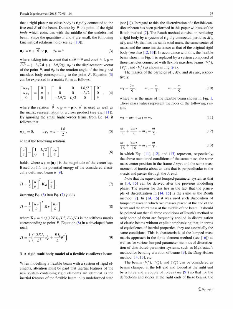
Fig. 2 The rigid multibodymodel of a cantilever flexiblebeam-three particle case
similar relations to Eq. (6) hold, that is,[
ui
θi
]=
[1 L/80 1
][uPi
θi
], i = 1,3,
[u2
θ2
]=
[1 L/40 1
][uP2
θ2
],
(14)
where the quantities ui , uPi, and θi correspond to the body
(V ∗i ).Thus, in the second phase of modelling, each of the flex-
ible beams is replaced by a system of three rigid masslessbeams as shown in Fig. 2(b). The first rigid beam corre-sponding to (V ∗
1 ) is fixed. The last rigid beam correspondingto (V ∗
1 ) is fixed to the first rigid beam corresponding to (V ∗2 )
so that they form one rigid beam denoted by (V2). Also, thelast rigid beam corresponding to (V ∗
2 ) is fixed to the firstrigid beam corresponding to (V ∗
3 ) so that they form one rigidbeam denoted by (V4). The rigid beams (V0), (V1), . . . , (V6)
shown in Fig. 2(b) are interconnected by the revolute andprismatic joints with appropriate springs in them (cylindri-cal spring in the prismatic joint and the spiral spring in therevolute joint) and the particles M1, M2, and M3 are rigidlyconnected to the corresponding beams. In the case of a pris-matic joint, the relative joint displacement qi represents therelative linear displacement of body (Vi) with respect to itspreceding adjacent body (Vi−1) measured along the jointaxis determined by the unit vector ei , while in the case ofa revolute joint this coordinate describes the relative rota-tion of body (Vi) with respect to (Vi−1) carried out aboutthe axis ei . The vector ei is fixed to the preceding adjacentbody (Vi−1). The displacements qi (i = 1, . . . ,6) are deter-mined by the following relations:
q1 = uP1 , q2 = θ1, q3 = uP2 , q4 = θ2,
q5 = uP3 , q6 = θ3. (15)
In accordance to the principle of equality of stiffnessproperties [1], the potential energy arising from elasticforces of the springs in the joints:
1
2
6∑i=1
ciq2i , (16)
is equal to the total potential energy of the beams (V ∗1 ),
(V ∗2 ), and (V ∗
3 ):
1
2
(768EIz
L3u2
P1+ 4EIz
Lθ2
1 + 96EIz
L3u2
P2+ 2EIz
Lθ2
2
+ 768EIz
L3u2
P3+ 4EIz
Lθ2
3
). (17)
The expression (17) is obtained by using the expression (9)and the fact that the lengths of the beams (V ∗
1 ), (V ∗2 ), and
(V ∗3 ) are L/4, L/2, and L/4, respectively (see Fig. 2(a)).
Finally, comparing Eqs. (16) and (17) yields the followingstiffnesses of the introduced springs in the joints:
c1 = c5 = 768EIz
L3, c2 = c6 = 4EIz
L,
c3 = 96EIz
L3, c4 = 2EIz
L.
(18)
In this way, a model of a flexible beam has been formed inthe form of rigid multibody system by which the motion ofthe flexible beam can be approximatively analysed. How-ever, as in the case with the modelling techniques presentedin [1–3, 5, 6], in order to obtain more accurate results itis necessary to use a large number of rigid bodies. In themethod presented in this paper this is achieved in the fol-lowing way. The beam is divided into n equal parts of lengthL/n (see Fig. 3(a)).
Forsch Ingenieurwes (2013) 77:95–104 99
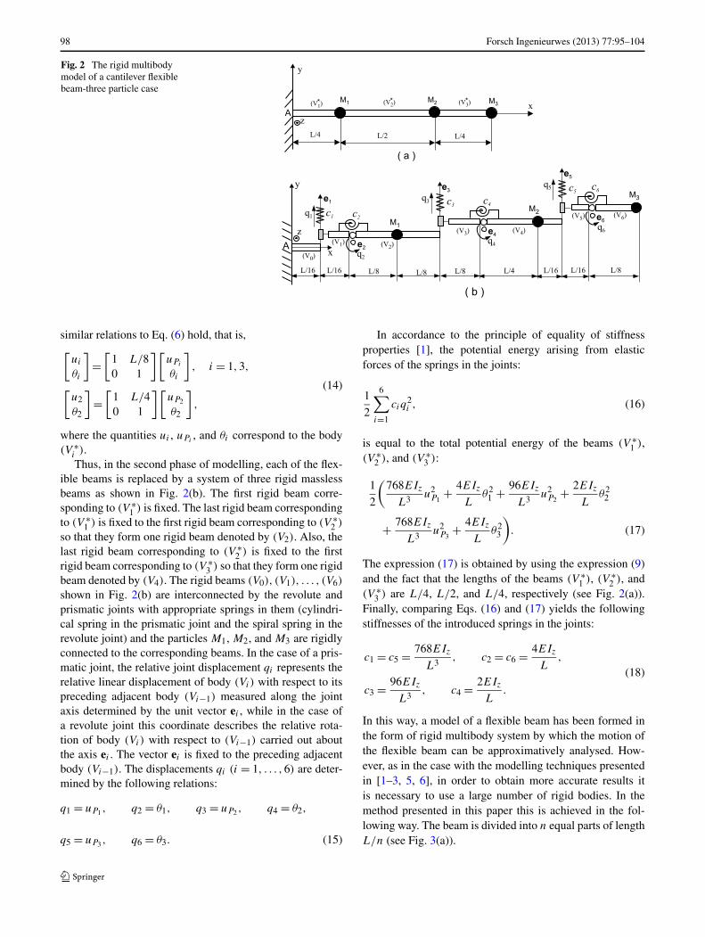
Fig. 3 The rigid multibodymodel of a cantilever flexiblebeam-3n particle case
Further, similar as in Fig. 2(a), each of these parts is re-placed with a system of three particles (see Fig. 3(b)) sothat a system of 3n particles M1, . . . ,M3n is obtained. Themasses of the particles, based on (10), are calculated as
m3i−2 = 5m
9n, m3i−1 = m
3n,
m3i = m
9n, i = 1, . . . , n.
(19)
In the last step, each of the massless flexible beams thatlink the particles is replaced by a system of three rigid beams(see Fig. 3(c)) in a manner similar to that in the case of threeparticles. After this we get a system of 6n+ 1 rigid masslessbeams to which 3n particles are rigidly connected as shownin Fig. 3(c) and where body (V0) is fixed. Now, based on(18), the stiffnesses of the springs in the joints of the multi-body system shown in Fig. 3(c) are calculated as:
c1+6i = c5+6i = 768n3EIz
L3,
c2+6i = c6+6i = 4nEIz
L,
c3+6i = 96n3EIz
L3,
c4+6i = 2nEIz
L, i = 0,1, . . . , n − 1.
(20)
Note that, as it can be seen in Figs. 2 and 3, the describedmethod, in its first step, is to a certain extent similar to thefinite element method. Namely, in the lumped finite elementmethod, the beam is divided into n finite elements and themass is concentrated at the ends of the elements (see e.g.[16]).
4 Linearised equations of motion and the eigenvalueproblem
The kinetic energy of the multibody system shown in Fig.3(c) is determined by:
T = 1
2
3n∑α=1
mαVMα · VMα (21)
where VMα is the velocity of the particle Mα . Introducing
the position vector rMα = −−→AMα of the particle Mα relative
to the inertial frame Axyz, the velocity VMα can be writtenas:
VMα = rMα =6n∑i=1
∂rMα
∂qi
qi (22)
where an overdot denotes the derivative with respect to timet . The partial derivatives ∂rMα/∂qi can be calculated as (seefor details [17, 18]):
∂rMα
∂qi
=⎧⎨⎩
χiei × (∑2α
r=i (pr + χrqrer ) + pMα) + χiei ,
i ≤ 2α
0, i > 2α
(23)
where 0 ∈ R3×1 is a zero vector, pr = −−→O�
r Or , pMα =−−−→O2αMα , and the points O�
i and Oi , belonging to beam (Vi),are placed on the axes of joints i and i + 1, respectively.The symbols χi and χi introduced in Eq. (23) representidentifiers of the joint type. If the ith joint is revolute, thenχi = 0, and if prismatic, then χi = 1. For symbol χi holdsthat χi = 1 − χi .
100 Forsch Ingenieurwes (2013) 77:95–104
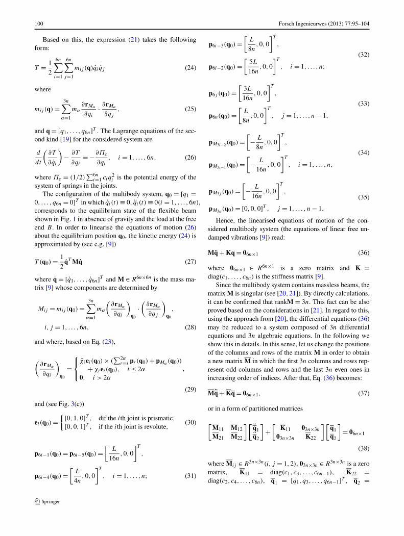
Based on this, the expression (21) takes the followingform:
T = 1
2
6n∑i=1
6n∑j=1
mij (q)qi qj (24)
where
mij (q) =3n∑
α=1
mα
∂rMα
∂qi
· ∂rMα
∂qj
, (25)
and q = [q1, . . . , q6n]T . The Lagrange equations of the sec-ond kind [19] for the considered system are
d
dt
(∂T
∂qi
)− ∂T
∂qi
= −∂Πc
∂qi
, i = 1, . . . ,6n, (26)
where Πc = (1/2)∑6n
i=1 ciq2i is the potential energy of the
system of springs in the joints.The configuration of the multibody system, q0 = [q1 =
0, . . . , q6n = 0]T in which qi (t) ≡ 0, qi(t) ≡ 0(i = 1, . . . ,6n),corresponds to the equilibrium state of the flexible beamshown in Fig. 1 in absence of gravity and the load at the freeend B . In order to linearise the equations of motion (26)about the equilibrium position q0, the kinetic energy (24) isapproximated by (see e.g. [9])
T (q0) = 1
2qT Mq (27)
where q = [q1, . . . , q6n]T and M ∈ R6n×6n is the mass ma-trix [9] whose components are determined by
Mij = mij (q0) =3n∑
α=1
mα
(∂rMα
∂qi
)q0
·(
∂rMα
∂qj
)q0
,
i, j = 1, . . . ,6n, (28)
and where, based on Eq. (23),
(∂rMα
∂qi
)q0
=⎧⎨⎩
χiei (q0) × (∑2α
r=i pr (q0) + pMα(q0))
+ χiei (q0), i ≤ 2α
0, i > 2α
,
(29)
and (see Fig. 3(c))
ei (q0) ={ [0,1,0]T , dif the ith joint is prismatic,
[0,0,1]T , if the ith joint is revolute,(30)
p6i−1(q0) = p6i−5(q0) =[
L
16n,0,0
]T
,
p6i−4(q0) =[
L
4n,0,0
]T
, i = 1, . . . , n; (31)
p6i−3(q0) =[
L
8n,0,0
]T
,
p6i−2(q0) =[
5L
16n,0,0
]T
, i = 1, . . . , n;(32)
p6j (q0) =[
3L
16n,0,0
]T
,
p6n(q0) =[
L
8n,0,0
]T
, j = 1, . . . , n − 1,
(33)
pM3i−2(q0) =[− L
8n,0,0
]T
,
pM3i−1(q0) =[− L
16n,0,0
]T
, i = 1, . . . , n,
(34)
pM3j(q0) =
[− L
16n,0,0
]T
,
pM3n(q0) = [0,0,0]T , j = 1, . . . , n − 1.
(35)
Hence, the linearised equations of motion of the con-sidered multibody system (the equations of linear free un-damped vibrations [9]) read:
Mq + Kq = 06n×1 (36)
where 06n×1 ∈ R6n×1 is a zero matrix and K =diag(c1, . . . , c6n) is the stiffness matrix [9].
Since the multibody system contains massless beams, thematrix M is singular (see [20, 21]). By directly calculations,it can be confirmed that rankM = 3n. This fact can be alsoproved based on the considerations in [21]. In regard to this,using the approach from [20], the differential equations (36)may be reduced to a system composed of 3n differentialequations and 3n algebraic equations. In the following weshow this in details. In this sense, let us change the positionsof the columns and rows of the matrix M in order to obtaina new matrix M in which the first 3n columns and rows rep-resent odd columns and rows and the last 3n even ones inincreasing order of indices. After that, Eq. (36) becomes:
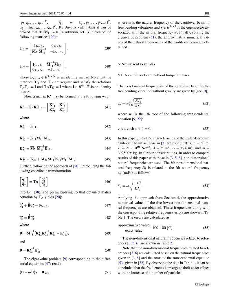
[q2, q4, . . . , q6n]T , q1 = [q1, q3, . . . , q6n−1]T ,q2 = [q2, q4, . . . , q6n]T . By directly calculating it can beproved that det M11 �= 0. In addition, let us introduce thefollowing matrices [20]:
TΛ =[
I3n×3n 03n×3n
M21M−111 −I3n×3n
], (39)
TΠ =[
I3n×3n M−111 M12
03n×3n −I3n×3n
], (40)
where I3n×3n ∈ R3n×3n is an identity matrix. Note that thematrices TΛ and TΠ are regular and satisfy the relationsTΛTΛ = I and TΠ TΠ = I where I ∈ R6n×6n is an identitymatrix.
Now, a matrix K� may be formed in the following way:
K� = TΛKTΠ =[
K�11 K�
12K�
21 K�22
], (41)
where
K�11 = K11, (42)
K�12 = K11M
−111 M12, (43)
K�21 = M21M
−111 K11, (44)
K�22 = K22 + M21M
−111 K11M
−111 M12. (45)
Further, following the approach of [20], introducing the fol-lowing coordinate transformation[
q1q2
]= TΠ
[q�
1q�
2
](46)
into Eq. (38), and premultiplying so that obtained matrixequation by TΛ yields [20]:
q�
1 + Bq�1 = 03n×1, (47)
q�2 = ˜Bq�
1, (48)
where
B = M−111
(K�
12K�−1
22 K�21 − K�
11
), (49)
and
˜B = K�−1
22 K�21. (50)
The eigenvalue problem [9] corresponding to the differ-ential equations (47) reads:
(B − ω2I
)v = 03n×1 (51)
where ω is the natural frequency of the cantilever beam infree bending vibrations and v ∈ R3n×1 is the eigenvector as-sociated with the natural frequency ω. Finally, solving theeigenvalue problem (51), the approximative numerical val-ues of the natural frequencies of the cantilever beam are ob-tained.
5 Numerical examples
5.1 A cantilever beam without lumped masses
The exact natural frequencies of the cantilever beam in thefree bending vibration without gravity are given by (see [9]):
ωi = w2i
√EIz
mL3(52)
where wi is the ith root of the following transcendentalequation [9, 22]:
cosw coshw + 1 = 0. (53)
In this paper, the same characteristics of the Euler-Bernoullicantilever beam as those in [3] are used, that is, L = 50 m,E = 21 · 1010 N/m2, A = π m2, Iz = π/4 m4, and m =392500π kg. In further considerations, in order to compareresults of this paper with those in [3, 5, 6], non-dimensionalnatural frequencies are used. The ith non-dimensional nat-ural frequency ωi is related to the ith natural frequencyωi (rad/s) as follows:
ωi = ωi
√mL3
EIz
. (54)
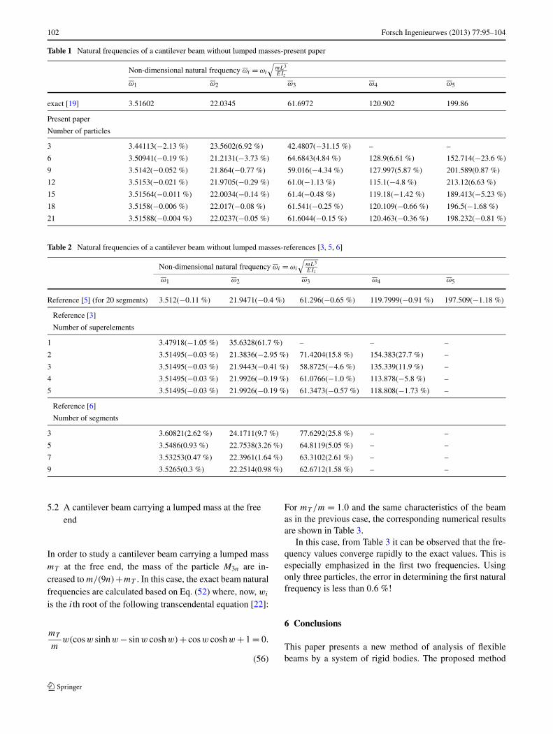
Applying the approach from Section 4, the approximativenumerical values of the five lowest non-dimensional natu-ral frequencies are obtained. These frequencies along withthe corresponding relative frequency errors are shown in Ta-ble 1. The errors are calculated as:
approximative value
exact value· 100–100 [%]. (55)
The non-dimensional natural frequencies related to refer-ences [3, 5, 6] are shown in Table 2.
Note that the non-dimensional frequencies related to ref-erences [3, 6] are calculated based on the natural frequenciesgiven in [3, 5] and the roots of the transcendental equation(53) given in [22]. By observing the data in Table 1, it can beconcluded that the frequencies converge to their exact valueswith the increase of a number of particles.
102 Forsch Ingenieurwes (2013) 77:95–104
Table 1 Natural frequencies of a cantilever beam without lumped masses-present paper
5.2 A cantilever beam carrying a lumped mass at the freeend
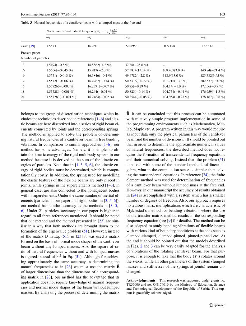
In order to study a cantilever beam carrying a lumped massmT at the free end, the mass of the particle M3n are in-creased to m/(9n)+mT . In this case, the exact beam naturalfrequencies are calculated based on Eq. (52) where, now, wi
is the ith root of the following transcendental equation [22]:
mT
mw(cosw sinhw − sinw coshw)+ cosw coshw + 1 = 0.
(56)
For mT /m = 1.0 and the same characteristics of the beamas in the previous case, the corresponding numerical resultsare shown in Table 3.
In this case, from Table 3 it can be observed that the fre-quency values converge rapidly to the exact values. This isespecially emphasized in the first two frequencies. Usingonly three particles, the error in determining the first naturalfrequency is less than 0.6 %!
6 Conclusions
This paper presents a new method of analysis of flexiblebeams by a system of rigid bodies. The proposed method
Forsch Ingenieurwes (2013) 77:95–104 103
Table 3 Natural frequencies of a cantilever beam with a lumped mass at the free end
belongs to the group of discretization techniques which in-cludes the techniques described in references [1–6] and elas-tic beams are here discretized into a series of rigid beam el-ements connected by joints and the corresponding springs.The method is applied to solve the problem of determin-ing natural frequencies of a cantilever beam in free bendingvibration. In comparison to similar approaches [1–6], ourmethod has some advantages. Namely, it is simpler to ob-tain the kinetic energy of the rigid multibody system in ourmethod because it is derived as the sum of the kinetic en-ergies of particles. Note that in [1–3, 5, 6], the kinetic en-ergy of rigid bodies must be determined, which is compu-tationally costly. In addition, the spring used for modellingthe elastic features of the flexible beams are only placed injoints, while springs in the superelements method [1–3], ingeneral case, are also connected to the nonadjacent bodieswithin superelements. Under the same number of inertial el-ements (particles in our paper and rigid bodies in [3, 5, 6]),our method has similar accuracy as the methods in [3, 5,6]. Under 21 particles, accuracy in our paper is higher inregard to all three references mentioned. It should be notedthat our method and the method presented in [23] are sim-ilar in a way that both methods are brought down to theformation of the eigenvalue problem (51). However, insteadof the matrix B in Eq. (51), in [23] it was used a matrixformed on the basis of normal mode shapes of the cantileverbeam without any lumped masses. Also the square of ra-tio of natural frequencies without and with lumped massesis figured instead of ω2 in Eq. (51). Although for achiev-ing approximately the same accuracy in determining thenatural frequencies as in [23] we must use the matrix Bof larger dimensions than the dimensions of a correspond-ing matrix in [23], our method has the advantage that itsapplication does not require knowledge of natural frequen-cies and normal mode shapes of the beam without lumpedmasses. By analysing the process of determining the matrix
B, it can be concluded that this process can be automatedwith relatively simple program implementation in some ofthe programming environments such as Mathematica, Mat-lab, Maple etc. A program written in this way would requireas input data only the physical parameters of the cantileverbeam and the number of divisions n. It should be pointed outthat in order to determine the approximate numerical valuesof natural frequencies, the described method does not re-quire the formation of transcendental frequency equationsand their numerical solving. Instead that, the problem (51)is solved with some of the standard methods of linear al-gebra, what in the computation sense is simpler than solv-ing the transcendental equations. In reference [24], the finiteelement method was used for determination of frequenciesof a cantilever beam without lumped mass at the free end.However, in our manuscript the accuracy of results obtainedin [24] is accomplished with a system which has a smallernumber of degrees of freedom. Also, our approach requiresno tedious matrix multiplications which are characteristic ofMyklestad’s method for bending vibration, where the useof the transfer matrix method results in the correspondingfrequency equation (see [9] for details). The method can bealso adapted to study bending vibrations of flexible beamswith various kind of boundary conditions at the ends such asclamped-clamped, clamped-pinned, pinned-pinned etc. Atthe end it should be pointed out that the models describedin Figs. 2 and 3 can be very easily adapted for the analysisof vibrations of the rotating cantilever beam. For that pur-pose, it is enough to take that the body (V0) rotates aroundthe z-axis, while all other parameters of the system (lumpedmasses and stiffnesses of the springs at joints) remain un-changed.
Acknowledgements This research was supported under grants no.TR35006 and no. ON174016 by the Ministry of Education, Scienceand Technological Development of the Republic of Serbia. This sup-port is gratefully acknowledged.
104 Forsch Ingenieurwes (2013) 77:95–104
References
1. Schiehlen WO, Rauh J (1986) Modeling of flexible multibeamsystems by rigid-elastic superelements. Rev Bras Cienc Mec8(2):151–163
2. Rauh J, Schiehlen WO (1987) Various approaches for the mod-elling of flexible robot arms. In: Elishahoff I, Irretier H (eds) Re-fined dynamical theories of beams, plates and shells and their ap-plications. Springer, Berlin, pp 420–429
3. Molenaarx DP, Sj D (1998) Modeling the structural dynamics ofthe lagerwey LW-50/750m wind turbine. Wind Eng 22(6):253–264
4. Zhao X, Maisser P, Wu J (2007) A new multibody modellingmethodology for wind turbine structures using a cardanic jointbeam element. Renew Energy 32:532–546
5. Wang Y, Huston RL (1994) A lumped parameter method in thenonlinear analysis of flexible multibody systems. Comput Struct50(3):421–432
6. Plosa J, Wojciech S (2000) Dynamics of systems with changingconfiguration and with flexible beam-like links. Mech Mach The-ory 35:1515–1534
7. Routh EJ (1905) Treatise on the dynamics of a system of rigidbodies, elementary part. Dover Publication Inc, New York
8. Dimentberg FM (1965) The screw calculus and its applications inmechanics. Nauka, Moscow (in Russian)
9. Meirovitch L (2001) Fundamentals of vibrations. McGraw-Hill,New York
11. Nikravesh PE (1988) Computer aided analysis of mechanical sys-tems. Prentice Hall, Englewood Cliffs
12. Attia HA, El-Mistikawy TMA (2001) A matrix formulation for thedynamic analysis of planar mechanisms using point coordinatesand velocity transformation. Eur J Mech A, Solids 20(6):981–995
13. Chaudhary H, Saha SK (2008) Balancing of shaking forces andshaking moments for planar mechanisms using the equimomentalsystems. Mech Mach Theory 43(3):310–334
14. Ding X, Selig JM, Zhan Q (2002) Study on dynamic modelingof compliant manipulators. In: 4th world congress on intelligentcontrol and automation, Shanghai, P.R. China, pp 1347–1353
15. Ding X, Selig JM (2004) Lumped parameter dynamic modellingfor the flexible manipulator. In: 5th world congress on intelligentcontrol and automation, Hangzhou, P.R. China, pp 280–284
16. Przemineiecki JS (1968) Theory of matrix structural analysis.McGraw-Hill, New York
17. Covic V, Lazarevic M (2009) Mechanics of robots. Faculty of Me-chanical Engineering, University of Belgrade (in Serbian)
18. Thomas M, Tesar D (1982) Dynamic modeling of serial manipu-lator arms. ASME J Dyn Syst Meas Control 104:218–228
19. Lurie AI (2002) Analytical mechanics. Springer, New York20. Belonozhko PA, Zhechev MM, Tarasov SV (1986) Mathematical
modeling of the dynamics of a system of two bodies coupled byan elastic multiple-element chain. Int Appl Mech 22(7):683–688
21. Zhechev MM (2007) Equations of motion for singular systems ofmassed and massless bodies. J Multibody Dyn 221:591–597
22. Laura PAA, Pombo JL, Susemihl EA (1974) A note on the vibra-tions of a clamped-free beam with a mass at the free end. J SoundVib 37(2):161–168
23. Wu JS, Lin TL (1990) Free vibration analysis of a uniform can-tilever beam with point masses by an analytical and numericalcombined method. J Sound Vib 136(2):201–213
24. Sehgal S, Kumar H (2012) Structural dynamic analysis of can-tilever beam structure. Int J Res Eng Appl Sci 2(2):1110–1114