econstor www.econstor.eu Der Open-Access-Publikationsserver der ZBW – Leibniz-Informationszentrum Wirtschaft The Open Access Publication Server of the ZBW – Leibniz Information Centre for Economics Standard-Nutzungsbedingungen: Die Dokumente auf EconStor dürfen zu eigenen wissenschaftlichen Zwecken und zum Privatgebrauch gespeichert und kopiert werden. Sie dürfen die Dokumente nicht für öffentliche oder kommerzielle Zwecke vervielfältigen, öffentlich ausstellen, öffentlich zugänglich machen, vertreiben oder anderweitig nutzen. Sofern die Verfasser die Dokumente unter Open-Content-Lizenzen (insbesondere CC-Lizenzen) zur Verfügung gestellt haben sollten, gelten abweichend von diesen Nutzungsbedingungen die in der dort genannten Lizenz gewährten Nutzungsrechte. Terms of use: Documents in EconStor may be saved and copied for your personal and scholarly purposes. You are not to copy documents for public or commercial purposes, to exhibit the documents publicly, to make them publicly available on the internet, or to distribute or otherwise use the documents in public. If the documents have been made available under an Open Content Licence (especially Creative Commons Licences), you may exercise further usage rights as specified in the indicated licence. zbw Leibniz-Informationszentrum Wirtschaft Leibniz Information Centre for Economics Franck, Raphaël; Galor, Oded Working Paper Is Industrialization Conducive to Long-Run Prosperity? IZA Discussion Papers, No. 9158 Provided in Cooperation with: Institute for the Study of Labor (IZA) Suggested Citation: Franck, Raphaël; Galor, Oded (2015) : Is Industrialization Conducive to Long-Run Prosperity?, IZA Discussion Papers, No. 9158 This Version is available at: http://hdl.handle.net/10419/114040
Transcript
econstor www.econstor.eu
Der Open-Access-Publikationsserver der ZBW – Leibniz-Informationszentrum WirtschaftThe Open Access Publication Server of the ZBW – Leibniz Information Centre for Economics
Standard-Nutzungsbedingungen:
Die Dokumente auf EconStor dürfen zu eigenen wissenschaftlichenZwecken und zum Privatgebrauch gespeichert und kopiert werden.
Sie dürfen die Dokumente nicht für öffentliche oder kommerzielleZwecke vervielfältigen, öffentlich ausstellen, öffentlich zugänglichmachen, vertreiben oder anderweitig nutzen.
Sofern die Verfasser die Dokumente unter Open-Content-Lizenzen(insbesondere CC-Lizenzen) zur Verfügung gestellt haben sollten,gelten abweichend von diesen Nutzungsbedingungen die in der dortgenannten Lizenz gewährten Nutzungsrechte.
Terms of use:
Documents in EconStor may be saved and copied for yourpersonal and scholarly purposes.
You are not to copy documents for public or commercialpurposes, to exhibit the documents publicly, to make thempublicly available on the internet, or to distribute or otherwiseuse the documents in public.
If the documents have been made available under an OpenContent Licence (especially Creative Commons Licences), youmay exercise further usage rights as specified in the indicatedlicence.
zbw Leibniz-Informationszentrum WirtschaftLeibniz Information Centre for Economics
Franck, Raphaël; Galor, Oded
Working Paper
Is Industrialization Conducive to Long-RunProsperity?
IZA Discussion Papers, No. 9158
Provided in Cooperation with:Institute for the Study of Labor (IZA)
Suggested Citation: Franck, Raphaël; Galor, Oded (2015) : Is Industrialization Conducive toLong-Run Prosperity?, IZA Discussion Papers, No. 9158
This Version is available at:http://hdl.handle.net/10419/114040
DI
SC
US
SI
ON
P
AP
ER
S
ER
IE
S
Forschungsinstitut zur Zukunft der ArbeitInstitute for the Study of Labor
Is Industrialization Conducive to Long-Run Prosperity?
Any opinions expressed here are those of the author(s) and not those of IZA. Research published in this series may include views on policy, but the institute itself takes no institutional policy positions. The IZA research network is committed to the IZA Guiding Principles of Research Integrity. The Institute for the Study of Labor (IZA) in Bonn is a local and virtual international research center and a place of communication between science, politics and business. IZA is an independent nonprofit organization supported by Deutsche Post Foundation. The center is associated with the University of Bonn and offers a stimulating research environment through its international network, workshops and conferences, data service, project support, research visits and doctoral program. IZA engages in (i) original and internationally competitive research in all fields of labor economics, (ii) development of policy concepts, and (iii) dissemination of research results and concepts to the interested public. IZA Discussion Papers often represent preliminary work and are circulated to encourage discussion. Citation of such a paper should account for its provisional character. A revised version may be available directly from the author.
IZA Discussion Paper No. 9158 June 2015
ABSTRACT
Is Industrialization Conducive to Long-Run Prosperity?* This research explores the long-run effect of industrialization on the process of development. In contrast to conventional wisdom that views industrial development as a catalyst for economic growth, the study establishes that while the adoption of industrial technology was conducive to economic development in the short-run, it has had a detrimental effect on standards of living in the long-run. Exploiting exogenous source of regional variation in the adoption of steam engines during the French industrial revolution, the research establishes that regions in which industrialization was more intensive experienced an increase in literacy rates more swiftly and generated higher income per capita in the subsequent decades. Nevertheless, intensive industrialization has had an adverse effect on income per capita, employment and equality by the turn of the 21st century. This adverse effect reflects neither higher unionization and wage rates nor trade protection, but rather underinvestment in human capital and lower employment in skilled-intensive occupations. These findings suggest that the characteristics that permitted the onset of industrialization, rather than the adoption of industrial technology per se, have been the source of prosperity among the currently developed economies that experienced an early industrialization. JEL Classification: N33, N34, O14, O33 Keywords: economic growth, industrialization, steam engine Corresponding author: Oded Galor Department of Economics Brown University 64 Waterman St. Providence, RI 02912 USA E-mail: [email protected]
* We thank Mario Carillo, Gregory Casey, Pedro Dal Bo, Martin Fiszbein, Marc Klemp, David Le Bris, Stelios Michalopoulos, Ömer Özak, Assaf Sarid, Yannai Spitzer, Uwe Sunde and David Weil for helpful discussions and participants in various seminars for comments. We thank Guillaume Daudin for sharing his data with us. Raphaël Franck wrote part of this paper as Marie Curie Fellow at the Department of Economics at Brown University under funding from the People Programme (Marie Curie Actions) of the European Union’s Seventh Framework Programme (FP 2007-2013) under REA Grant agreement PIOF-GA-2012- 327760 (TCDOFT).
The process of development has been marked by reversals as well as persistence in the relative
wealth of nations. While some geographical characteristics that were conducive for economic de-
velopment in the agricultural stage had detrimental effects on the transition to the industrial stage
of development, conventional wisdom suggests that prosperity has persisted among societies that
experienced an earlier industrialization (Landes, 1998; Maddison, 2001; Galor, 2011).
Regional development within advanced economies, nevertheless, appears far from being indica-
tive of the presence of a persistent beneficial effect of early industrialization. In particular, anecdotal
evidence suggests that regions which were prosperous industrial centers in Western Europe and in
the Americas in the 19th century (e.g., the Rust Belt in the USA, the Midlands in the UK, and the
Ruhr valley in Germany) have experienced a reversal in their comparative development.
These conflicting observations about the long-run effect of industrialization on the prosperity of
regions and nations may suggest that factors which fostered industrial development in the Western
world, rather than the forces of industrialization per se, are associated with the persistence of
fortune across these industrial nations. In particular, the delayed industrialization of some currently
leading economies suggests that it is not inconceivable that the process of industrialization, despite
its earlier virtues, has had detrimental effects on the transition to the post-industrial stage of
development.
The research explores the long-run effect of industrialization on the process of development.
In contrast to conventional wisdom that views industrial development as a catalyst for economic
growth, highlighting its persistent effect on economic prosperity, the study establishes that while
the adoption of industrial technology was initially conducive for economic development, it has had
a detrimental effect on standards of living in the long-run.
The study utilizes French regional data from the second half of the 19th century until the
beginning of the 21st century to explore the impact of the adoption of industrial technology on
the evolution of income per capita and human capital formation. It establishes that regions which
industrialized more intensively experienced an increase in literacy rates more swiftly and generated
higher income per capita in the subsequent decades. Nevertheless, industrialization has had an
adverse effect on income per capita, employment and equality by the turn of the 21st century.
The observed relationship between industrialization and economic development may reflect
the potential effect of industrialization on economic prosperity, the impact of development on
industrialization, as well as the influence of additional factors (e.g., institutional, cultural and
human capital characteristics). Thus, the research exploits exogenous regional variations in the
adoption of steam engines across France to establish the effect of industrialization on the process
of development.
In light of the association between industrialization and the intensity of the use of the steam
1
engine (Mokyr, 1990; Bresnahan and Trajtenberg, 1995; Rosenberg and Trajtenberg, 2004), the
study takes advantage of historical evidence regarding the regional diffusion of the steam engine
(Ballot, 1923; See, 1925; Leon, 1976) to identify the effect of regional variations in the intensity
of the use steam engine in 1860-1865 on the process of development. In particular, it exploits
the distances of each French department from Fresnes-sur-Escaut, where a steam engine was first
operated for commercial use in 1732, as exogenous source of variations in industrialization across
French regions.
Indeed, in line with the historical account, the distribution of steam engines across French
departments is indicative of a local diffusion process from Fresnes-sur-Escaut. Accounting for
confounding geographical and institutional characteristics, pre-industrial development as well as
distances from major economic centers, if the distance of a department away from Fresnes-sur-
Escaut was to increase from the 25th (337 km) to the 75th percentile (680 km) of the distance
distribution, this department would experience an aggregate drop of 97 hp (relative to a sample to
a sample mean of 655 hp).
The validity of the distance from Fresnes-sur-Escaut as an instrumental variable for the in-
tensity of the adoption of steam engines across France is enhanced by third additional factors.
First, conditional on the distance from Fresnes-sur-Escaut, distances between each department and
major centers of economic power in 1860-1865 (e.g., Paris, Marseille, Lyon, Rouen, Mulhouse, Bor-
deaux) are uncorrelated with the intensive use of the steam engine over this period. Second, the
distance from Fresnes-sur-Escaut is uncorrelated with economic development across France in the
pre-industrial period. Third, it appears that the Nord department had neither superior human
capital characteristics nor higher standard of living in comparison to the average department in
France.
The study establishes that the horse power of steam engines in industrial production in the
1860-1865 period had a positive and significant impact on income per capita in 1872, 1901 and 1930.
In particular, if a department had increased its total horse power of steam engines in 1860-1865 from
the 25th to the 75th percentile of the distribution, it would have experienced an increase in GDP
per capita of 79.1 percent in 1872, 159.6 percent in 1901 and 66.7 percent in 1930. Nevertheless,
industrialization had an adverse effect on income per capita, human capital formation, employment
and equality in the post-2000 period. In particular, if a department had experienced a increase in
its horse power in 1860-1865 from the 25th to the 75th percentile of the distribution, this increase
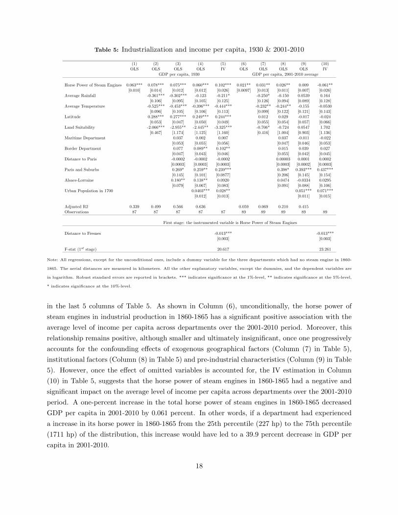
would have led to a 39.9 percent decrease in GDP per capita in 2001-2010.
It is important to note that the IV estimation reverses the OLS estimates of the relation-
ship between industrialization and the long-run level of income per capita from a positive to a
negative one. This reversal suggests that factors which fostered industrial development, rather
than industrialization per se, contributed to the positive association between industrialization and
long-run development. In particular, once one accounts for the effect of these omitted factors,
2
industrialization has an adverse effect on the standard of living in the long-run.
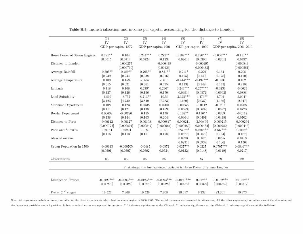
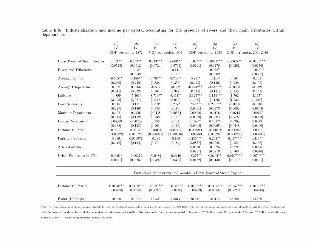
The empirical analysis accounts for a wide range of exogenous confounding geographical and
institutional characteristics, as well as for pre-industrial development, which may have contributed
to the relationship between industrialization and economic development. First, it accounts for
the potentially confounding impact of exogenous geographical characteristics of each of the French
departments on the relationship between industrialization and economic development. In particular,
it captures the potential effect of these geographical factors on the profitability of the adoption of
the steam engine, the pace of its regional diffusion, as well as on productivity and thus the evolution
of income per capita in the process of development. Second, it captures the potentially confounding
effects of the location of departments (i.e., latitude, border departments, maritime departments,
departments at a greater distance from the concentration of political power in Paris, and those that
were temporarily under German domination) on the diffusion of the steam engine and the diffusion
of development. Third, the analysis accounts for the differential level of development across France
in the pre-industrial era that may have affected jointly the process of development and the process
of industrialization. In particular, it controls for the effect of pre-industrial development on the
adoption of the steam engine and, independently, on the persistence of development.
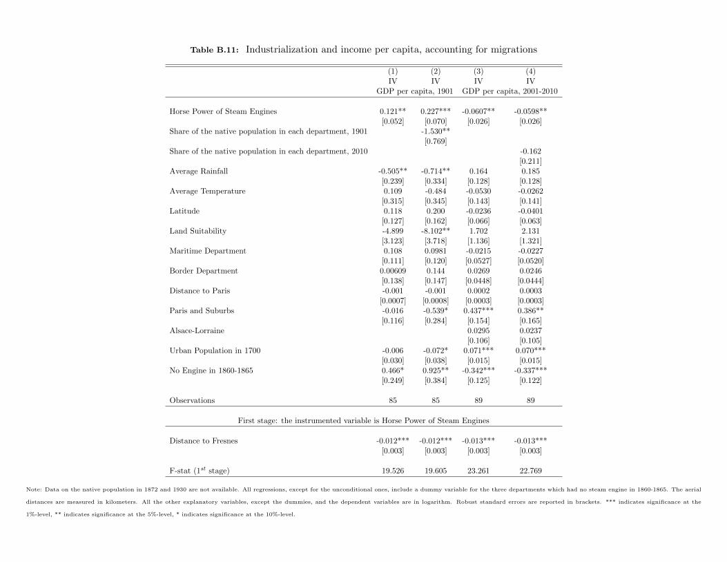
The research further explores the mediating channels through which earlier industrial develop-
ment has an adverse effect of the contemporary level of development. It establishes that the adverse
long-run effect of industrialization on the formation of human capital, beyond basic literacy skills, is
the underlining force that brought about the relative demise of the industrial regions. In contrast,
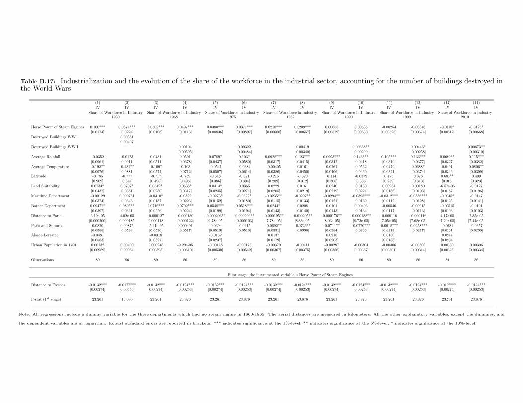
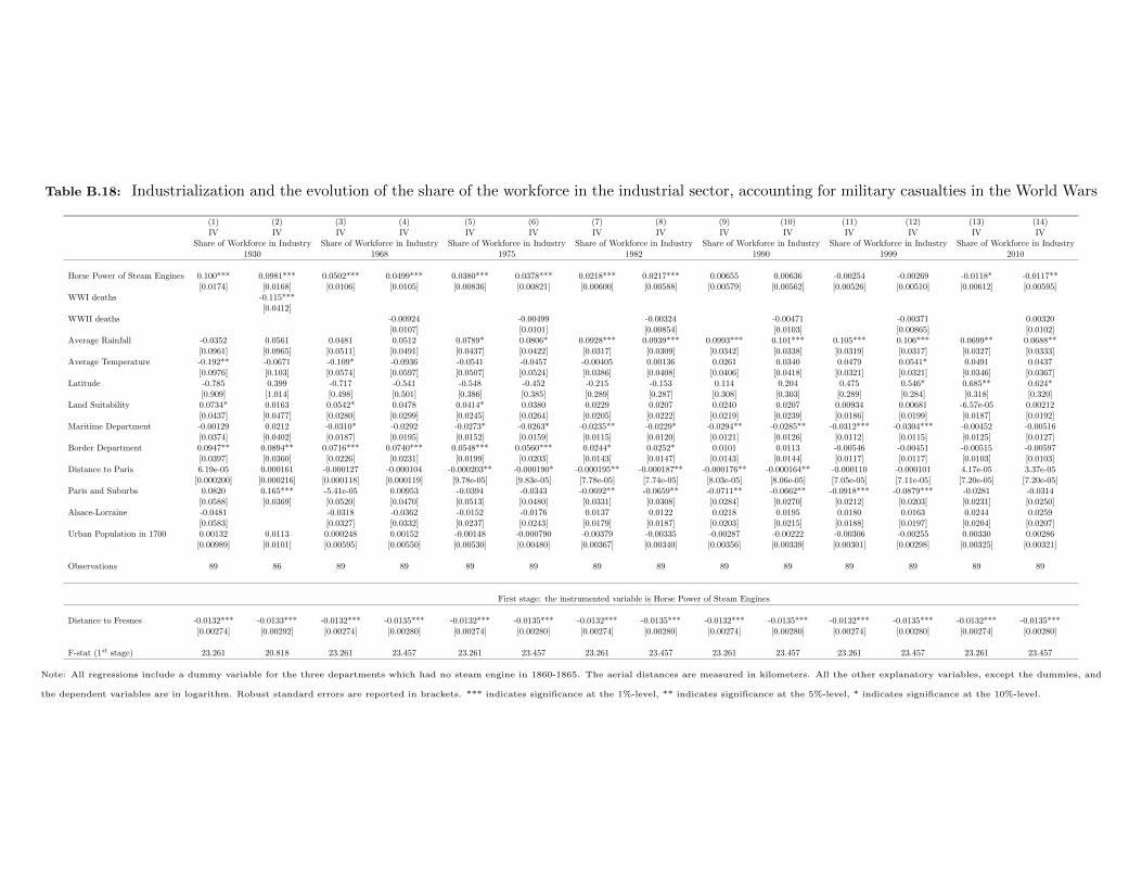
greater unionization, higher wages and trade protection in these industrial regions during their
economic prosperity, as well as destruction in the two world wars, did not contribute to their cur-
rent decline. Moreover, their decline cannot be attributed to variations in employment rates in the
service sector, but rather to the detrimental effect on the share of employment in skilled-intensive
occupations.
The remainder of this paper is as follows. Section 2 presents our data. Section 3 discusses
our empirical strategy. Section 4 presents our main results and our robustness checks. Section 5
assesses the relevance of potential mechanisms for these findings and Section 6 offers concluding
remarks.
2 Data and Main Variables
France was among the first countries to industrialize in Europe in the 18th century and its in-
dustrialization continued during the 19th century. Nevertheless, by 1914, the living standard in
France remained below that of England and of Germany, which had become the leading industrial
country in continental Europe. The slower path of industrialization in France has been attributed
to the consequences of the French Revolution (e.g., wars, legal reforms and land redistribution), the
3
patterns of domestic and foreign investment, cultural preferences for public services, as well as the
comparative advantage of France in agriculture vis-a-vis England and Germany (see the discussion
in, e.g., Levy-Leboyer and Bourguignon, 1990; Grantham, 1997; Crouzet, 2003).
This section examines the evolution of industrialization and income across 89 French depart-
ments, based on the administrative division of France in the 1860-1865 period, accounting for the
geographical and the institutional characteristics of these regions. The initial partition of the French
territory in 1790 was designed to ensure that the travel distance by horse from any location within
the department to the main administrative center would not exceed one day. The initial territory
of each department was therefore orthogonal to the process of development and the subsequent
minor changes in the borders of some departments did not reflect the effect of industrialization.
In particular, several departments that were split into smaller units are aggregated into their
historical territorial borders and regions that were temporarily removed from the French territory
are excluded from the analysis during those time periods.1 In light of the changes in the internal and
external boundaries of the French territory during the period of study, the number of departments
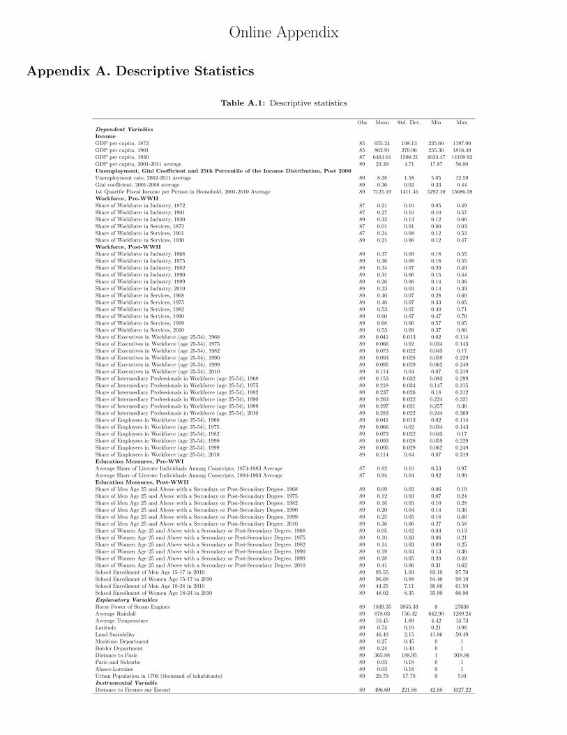
that is included in different stages of the analysis varies from 81 to 89. Table A.1 reports the
descriptive statistics for the variables in the empirical analysis across these departments.
2.1 Past and Present Measures of Income, Workforce and Human Capital
2.1.1 Income, unemployment and inequality
This study seeks to examine the effect of industrialization on the evolution of income per capita
in the process of development. Given that the industrial survey which is the basis for our analysis
was conducted between 1860 and 1865, the relevant data to capture the short-run and medium-run
effects of industrialization on income per capita are provided at the departmental level prior to
WWII for the years 1872, 1886, 1901, 1911 and 1930 by (Combes et al., 2011; Caruana-Galizia,
2013). Thus, for the sake of brevity, and equal spacing between those years, the analysis focuses
on income per capita in 1872, 1901 and 1930.
To assess the effects of industrialization on income per capita in the long-run, the analysis
is restricted to the 2001-2010 period, since data on income per capita at the departmental level
is only available in the post-1995 period and the corresponding data for the other indicators of
the standards of living only in the post-2001 period (INSEE - Institut National de la Statistique et
1The Parisian region encompassed three departments (Seine, Seine-et-Marne and Seine-et-Oise) before 1968 andit was split into eight (Essonne, Hauts-de-Seine, Paris, Seine-et-Marne, Seine-Saint-Denis, Val-de-Marne, Val d’Oiseand Yvelines) afterwards. Likewise, the Corsica department was split in 1975 into Corse-du-Sud and Haute-Corse.The three departments (i.e., Bas-Rhin, Haut-Rhin and Meurthe) which were under German rule between 1871 and1918 are excluded from the analysis of economic development over that time period. In addition, in the examinationof the robustness of the analysis with data prior to 1860, the three departments (i.e., Alpes-Maritimes, Haute-Savoieand Savoie) that were not part of France are excluded from the analysis.
4
des Etudes Economiques).2 Moreover, to lessen the potential impact of fluctuations in income per
capita, the effect of industrialization in the long-run is captured by its differential impact on the
average GDP per capita across departments over the 2001-2010 period.
Furthermore, the analysis examines the effect of industrialization on additional indicators of
economic development, unemployment and inequality. The data on unemployment are available
across departments over the 2002-2011 period, those on inequality over the 2001-2008 period,
and those on the main quartiles of the income distribution over the 2001-2010 period.3 Hence,to
lessen the potential impact of yearly fluctuations, the effect of industrialization on these economic
indicators is captured by their average values over the relevant time periods.
2.1.2 Workforce
The effect of industrialization on the sectoral composition of the workforce in the post-1860 period
is captured by the impact on the shares of employment in the agricultural, industrial and service
sectors. The surveys which capture the short-run and mid-run effects of industrialization are
those undertaken in 1872, 1901 and 1930 (Statistique Generale de la France). Similarly, to assess
the effects of industrialization on the sectoral composition in the post-WWII period, all available
surveys of the French population across departments (i.e., 1968, 1975, 1982, 1990, 1999 and 2010)
are used (INSEE - Institut National de la Statistique et des Etudes Economiques).
2.1.3 Human capital
The study further explores the effect of industrialization on the evolution of human capital in the
process of development. The effect of industrialization on human capital formation in the pre-WWI
period is captured by its impact on the literacy rates of French army conscripts (i.e., 20-year-old men
who reported for military service in the department where their father lived - Annuaire Statistique
De La France (1878-1939)). In particular, given the data limitations, the analysis focuses on the
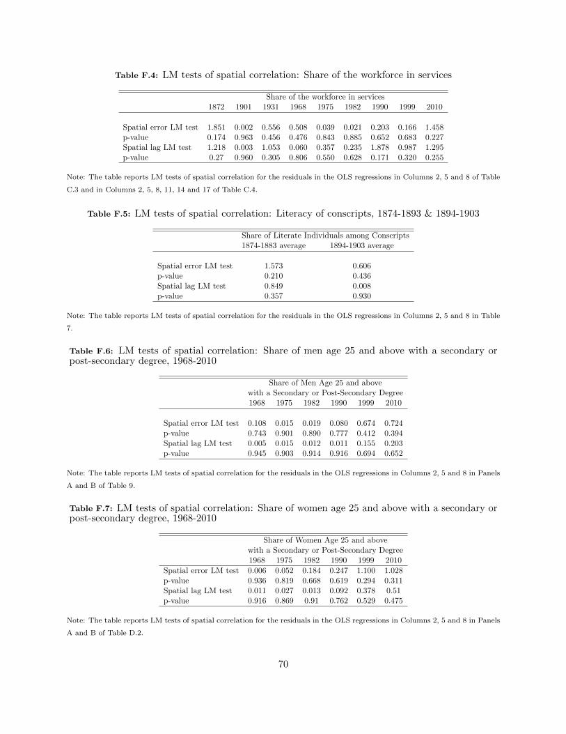
share of the literate conscripts over the 1874-1883 and 1894-1903 decades. As reported in Table
A.1, 82.0% of the French conscripts were literate over the 1874-1883 period and 94.1% over the
1894-1903 period.4
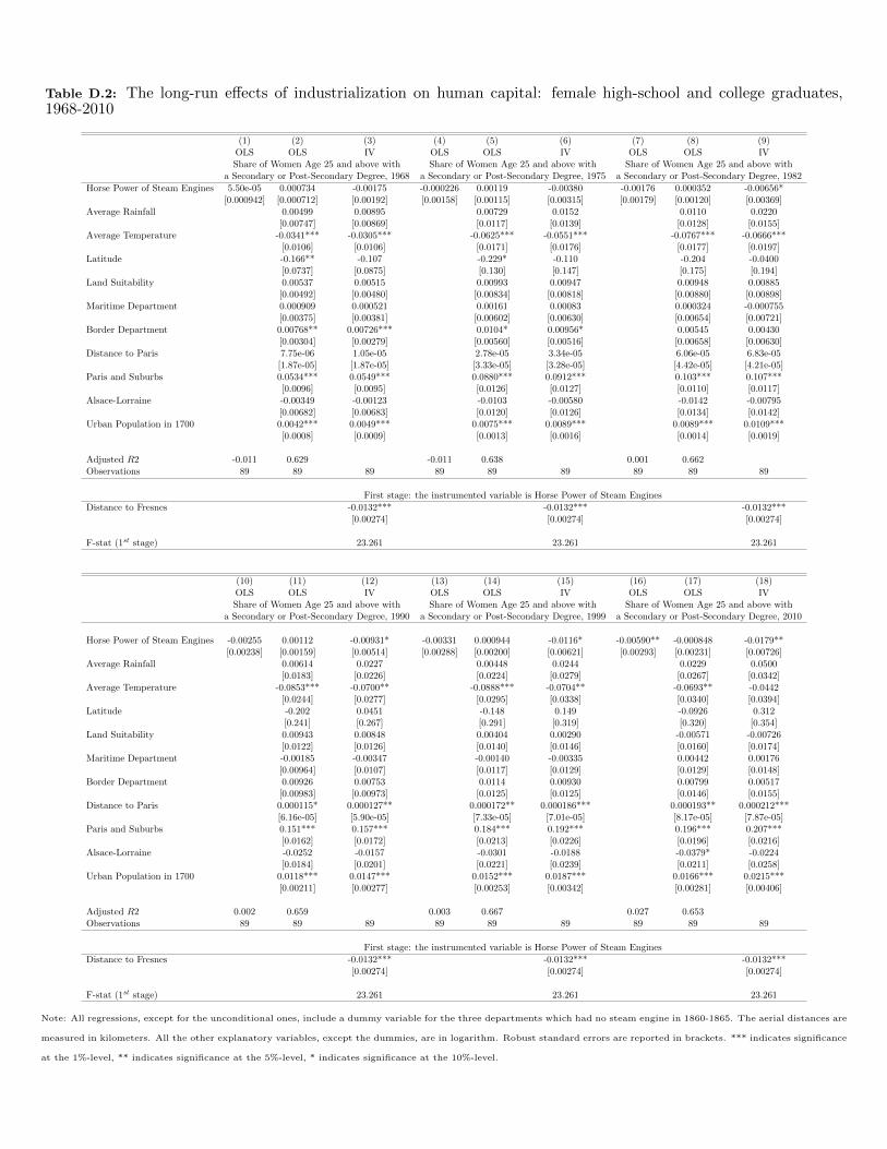
The effect of industrialization on human capital formation in the post-WWII period is captured
by its impact on the share of men and women (age 25 and above) who completed high-school as
reported in the available surveys of the French population across departments (i.e., 1968, 1975,
2The qualitative results remain unchanged if one considers the average income per capita over the entire sampleperiod available, 1995-2010.
3The income data are based on gross income, prior to state benefits, per person in a household.4In line with the historical evidence (e.g., Grew and Harrigan, 1991; Diebolt et al., 2005; Diebolt and Fontvieille,
2001), as reported in Table A.1, a sizeable share of the French population was literate even before the passing of the1881-1882 laws which made primary school attendance “free”and mandatory for boys and girls until age 13.
5
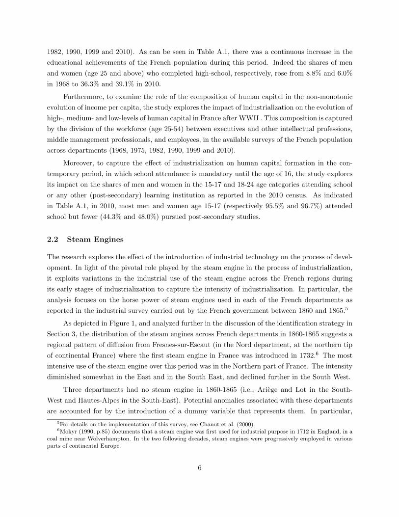
1982, 1990, 1999 and 2010). As can be seen in Table A.1, there was a continuous increase in the
educational achievements of the French population during this period. Indeed the shares of men
and women (age 25 and above) who completed high-school, respectively, rose from 8.8% and 6.0%
in 1968 to 36.3% and 39.1% in 2010.
Furthermore, to examine the role of the composition of human capital in the non-monotonic
evolution of income per capita, the study explores the impact of industrialization on the evolution of
high-, medium- and low-levels of human capital in France after WWII . This composition is captured
by the division of the workforce (age 25-54) between executives and other intellectual professions,
middle management professionals, and employees, in the available surveys of the French population
across departments (1968, 1975, 1982, 1990, 1999 and 2010).
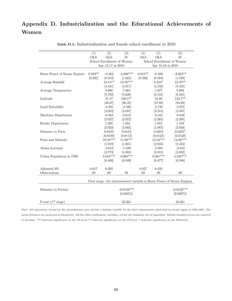
Moreover, to capture the effect of industrialization on human capital formation in the con-
temporary period, in which school attendance is mandatory until the age of 16, the study explores
its impact on the shares of men and women in the 15-17 and 18-24 age categories attending school
or any other (post-secondary) learning institution as reported in the 2010 census. As indicated
in Table A.1, in 2010, most men and women age 15-17 (respectively 95.5% and 96.7%) attended
school but fewer (44.3% and 48.0%) pursued post-secondary studies.
2.2 Steam Engines
The research explores the effect of the introduction of industrial technology on the process of devel-
opment. In light of the pivotal role played by the steam engine in the process of industrialization,
it exploits variations in the industrial use of the steam engine across the French regions during
its early stages of industrialization to capture the intensity of industrialization. In particular, the
analysis focuses on the horse power of steam engines used in each of the French departments as
reported in the industrial survey carried out by the French government between 1860 and 1865.5
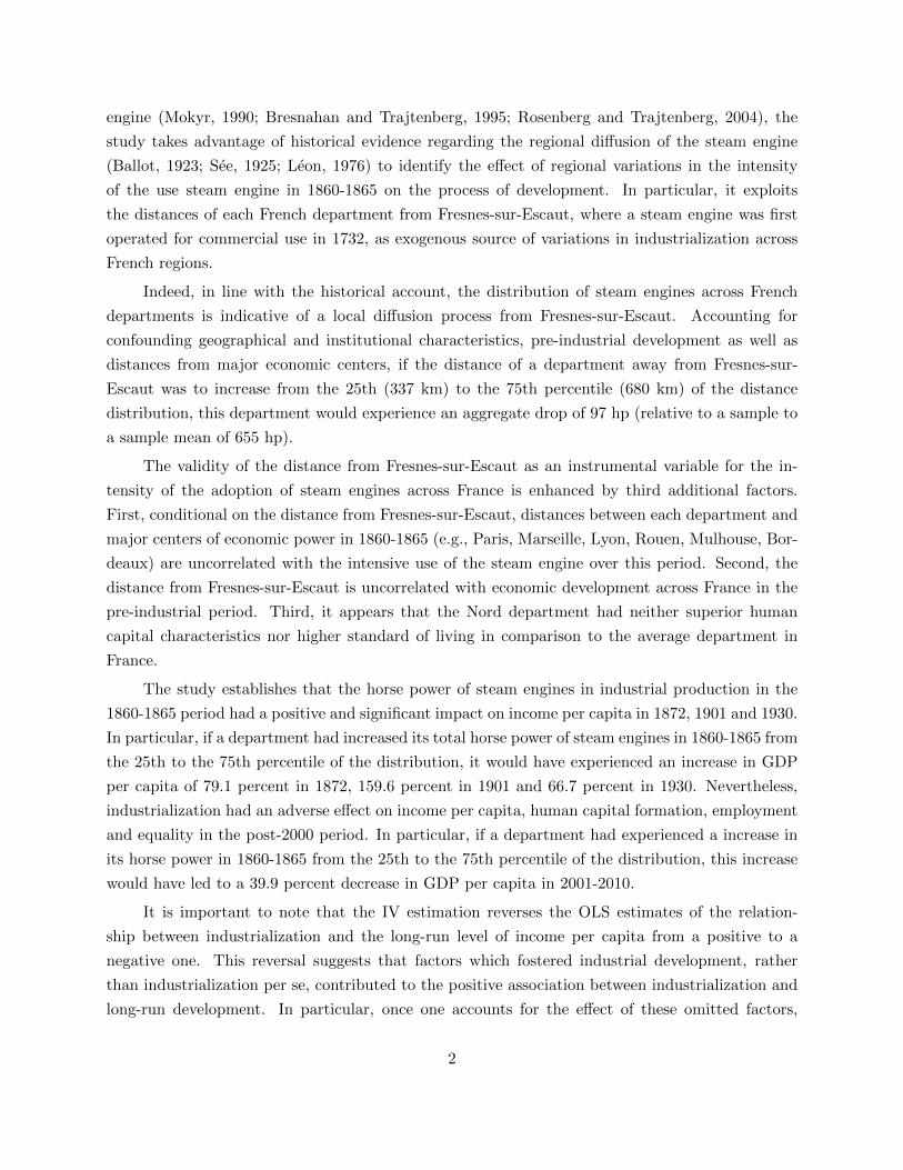
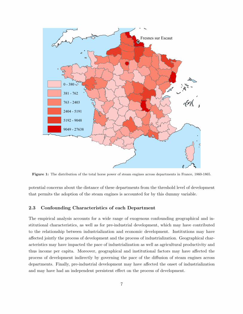
As depicted in Figure 1, and analyzed further in the discussion of the identification strategy in
Section 3, the distribution of the steam engines across French departments in 1860-1865 suggests a
regional pattern of diffusion from Fresnes-sur-Escaut (in the Nord department, at the northern tip
of continental France) where the first steam engine in France was introduced in 1732.6 The most
intensive use of the steam engine over this period was in the Northern part of France. The intensity
diminished somewhat in the East and in the South East, and declined further in the South West.
Three departments had no steam engine in 1860-1865 (i.e., Ariege and Lot in the South-
West and Hautes-Alpes in the South-East). Potential anomalies associated with these departments
are accounted for by the introduction of a dummy variable that represents them. In particular,
5For details on the implementation of this survey, see Chanut et al. (2000).6Mokyr (1990, p.85) documents that a steam engine was first used for industrial purpose in 1712 in England, in a
coal mine near Wolverhampton. In the two following decades, steam engines were progressively employed in variousparts of continental Europe.
6
0 - 380
381 - 762
763 - 2403
2404 - 5191
5192 - 9048
9049 - 27638
Fresnes sur Escaut
Figure 1: The distribution of the total horse power of steam engines across departments in France, 1860-1865.
potential concerns about the distance of these departments from the threshold level of development
that permits the adoption of the steam engines is accounted for by this dummy variable.
2.3 Confounding Characteristics of each Department
The empirical analysis accounts for a wide range of exogenous confounding geographical and in-
stitutional characteristics, as well as for pre-industrial development, which may have contributed
to the relationship between industrialization and economic development. Institutions may have
affected jointly the process of development and the process of industrialization. Geographical char-
acteristics may have impacted the pace of industrialization as well as agricultural productivity and
thus income per capita. Moreover, geographical and institutional factors may have affected the
process of development indirectly by governing the pace of the diffusion of steam engines across
departments. Finally, pre-industrial development may have affected the onset of industrialization
and may have had an independent persistent effect on the process of development.
7
2.3.1 Geographic Characteristics
0.21 - 0.58
0.59 - 0.74
0.75 - 0.82
0.83 - 0.92
0.93 - 0.98
Land Suitability.
642.9 - 750.2
750.3- 808.2
808.3 - 899.8
899.9 - 1002.9
1003.0 - 1289.2
Average Rainfall.
4.42 - 6.34
6.35 - 9.06
9.07 - 10.52
10.53 - 11.87
11.88 - 13.73
Average Temperature
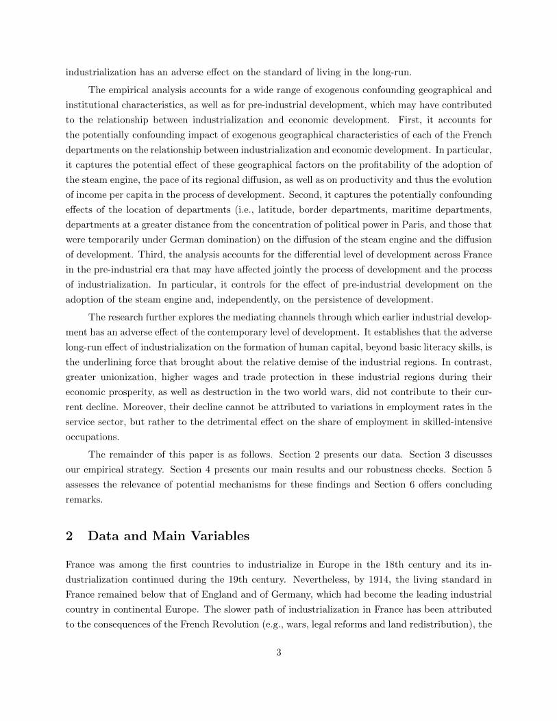
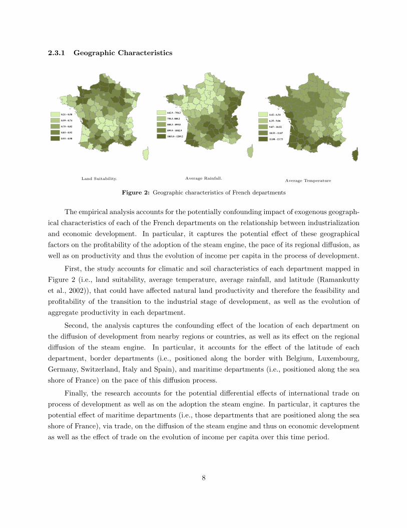
Figure 2: Geographic characteristics of French departments
The empirical analysis accounts for the potentially confounding impact of exogenous geograph-
ical characteristics of each of the French departments on the relationship between industrialization
and economic development. In particular, it captures the potential effect of these geographical
factors on the profitability of the adoption of the steam engine, the pace of its regional diffusion, as
well as on productivity and thus the evolution of income per capita in the process of development.
First, the study accounts for climatic and soil characteristics of each department mapped in
Figure 2 (i.e., land suitability, average temperature, average rainfall, and latitude (Ramankutty
et al., 2002)), that could have affected natural land productivity and therefore the feasibility and
profitability of the transition to the industrial stage of development, as well as the evolution of
aggregate productivity in each department.
Second, the analysis captures the confounding effect of the location of each department on
the diffusion of development from nearby regions or countries, as well as its effect on the regional
diffusion of the steam engine. In particular, it accounts for the effect of the latitude of each
department, border departments (i.e., positioned along the border with Belgium, Luxembourg,
Germany, Switzerland, Italy and Spain), and maritime departments (i.e., positioned along the sea
shore of France) on the pace of this diffusion process.
Finally, the research accounts for the potential differential effects of international trade on
process of development as well as on the adoption the steam engine. In particular, it captures the
potential effect of maritime departments (i.e., those departments that are positioned along the sea
shore of France), via trade, on the diffusion of the steam engine and thus on economic development
as well as the effect of trade on the evolution of income per capita over this time period.
8
2.3.2 Institutional Characteristics
The analysis deals with the effect of variations in the adoption of the steam engine across French
departments on their comparative development. This empirical strategy ensures that institutional
factors that were unique to France as a whole over this time period are not the source of the
differential pattern of development across these regions. Nevertheless, two regions of France over
this time period had a unique exposure to institutional characteristics that may have contributed
to the observed relationship between industrialization and economic development.
First, the emergence of state centralization in France, centuries prior to the process of in-
dustrialization, and the concentration of political power in Paris, may have affected differentially
the political culture and economic prosperity in Paris and its suburbs (i.e., Seine, Seine-et-Marne
and Seine-et-Oise). Hence, the empirical analysis includes a dummy variable for these three de-
partments, accounting for their potential confounding effects on the observed relationship between
industrialization and economic development, in general, and the adoption of the steam engine, in
particular. Moreover, the analysis captures the potential decline in the grip of the central govern-
ment in regions at a greater distance from Paris, and the diminished potential diffusion of develop-
ment into these regions, accounting for the effect of the aerial distance between the administrative
center of each department and Paris.
Second, the relationship between industrialization and development in the Alsace-Lorraine
region (i.e., the Bas-Rhin, Haut-Rhin and the Moselle departments) that was under German dom-
ination in the 1871-1918 period may represent the persistence of institutional and economic char-
acteristics that reflected their unique experience.7 Hence, the empirical analysis includes a dummy
variable for these regions, accounting for the confounding effects of the characteristics of the region.
2.3.3 Pre-Industrial Development
The differential level of development across France in the pre-industrial era may have affected
jointly the process of development and the process of industrialization. In particular, it may have
affected the adoption of the steam engine and it may have generated, independently, a persistent
effect on the process of development. Hence, the empirical analysis accounts for the potentially
confounding effects of the level of development in the pre-industrial period, more than 150 years
prior to the 1860-1865 industrial survey. This early level of development is captured by the degree
of urbanization (i.e., population of urban centers with more than 10,000 inhabitants) in each French
department in 1700 (Lepetit, 1994).8
7Differences in the welfare laws and labor market regulations in Alsace-Lorraine and the rest of France persistedthroughout most of the 20th century (see, e.g., Chemin and Wasmer, 2009). The laws on the separation of Churchand State are also different, and these differences were reaffirmed by a decision of the Supreme French ConstitutionalCourt in 2013 (Decision 2012-297 QPC, 21 February 2013).
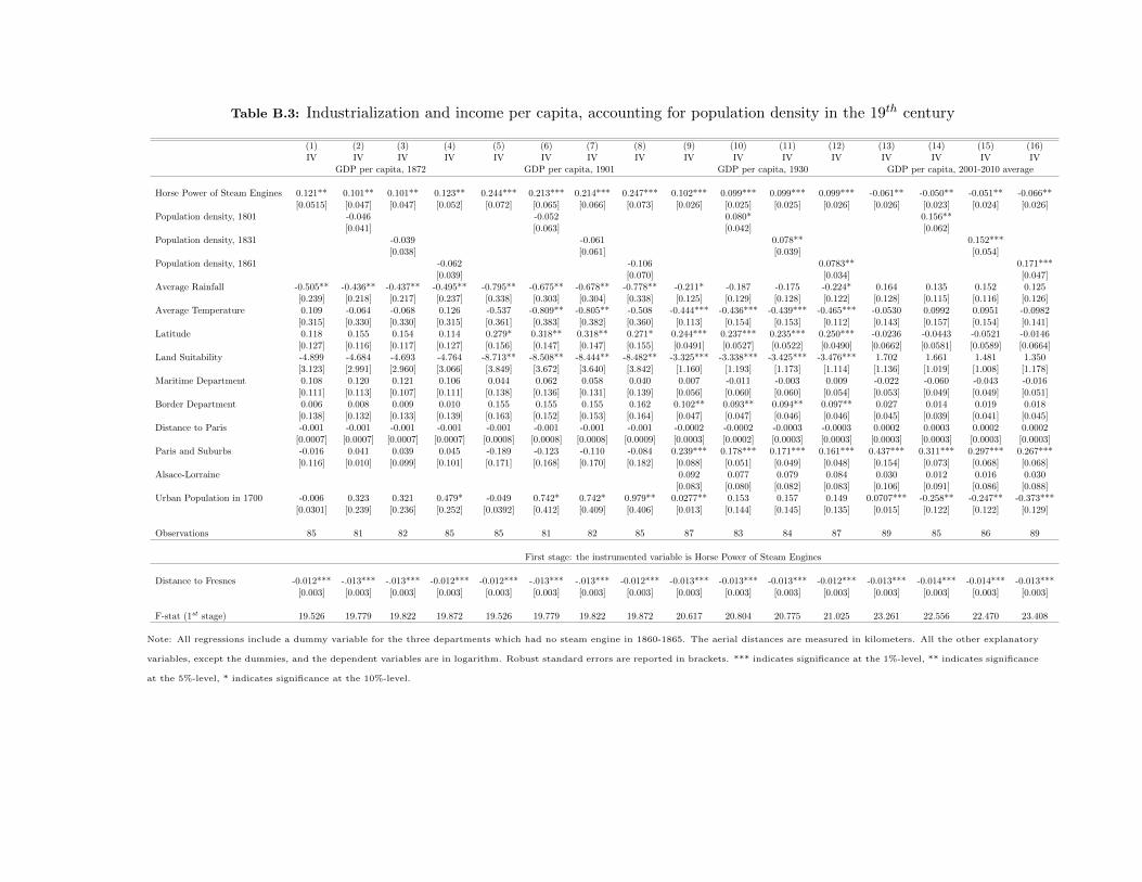
8The qualitative analysis remains intact if the potential effect of past population density is accounted for.
9
3 Empirical Methodology
3.1 Empirical Strategy
The observed relationship between industrialization and economic development is not necessarily
indicative of the causal effect of industrialization on economic prosperity. It may reflect the impact
of economic development on the process of industrialization as well as the influence of institutional,
geographical, cultural and human capital characteristics on the joint evolution of process of de-
velopment and the onset of industrialization. In light of the endogeneity of industrialization and
economic development, this research exploits exogenous regional variations in the adoption of the
steam engine across France to establish the effect of industrialization on the process of development.
The identification strategy is motivated by the historical account of the gradual regional
diffusion of the steam engine in France during the 18th and 19th century (Ballot, 1923; See, 1925;
Leon, 1976).9 Considering the positive association between industrialization and the intensity
in the use of the steam engine (Mokyr, 1990; Bresnahan and Trajtenberg, 1995; Rosenberg and
Trajtenberg, 2004), the study takes advantage of the regional diffusion of the steam engine to
identify the effect of local variations in the intensity of the use of the steam engine during the 1860-
1865 period on the process of development. In particular, it exploits the distances between each
French department and Fresnes-sur-Escaut (in the Nord department), where the first commercial
application of the steam engine across France was made in 1732, as an instrument for the use of
the steam engines in 1860-1865.10
Consistent with the diffusion hypothesis, the second steam engine in France that was utilized
for commercial purposes was operated in 1737 in the mines of Anzin, also in the Nord department,
less than 10 km away from Fresnes-sur-Escaut. Furthermore, in the subsequent decades till the
French Revolution the commercial use of the steam engine expanded predominantly to the nearby
northern and north-western regions. Nevertheless, at the onset of the French revolution in 1789,
steam engines were less widespread in France than in England. A few additional steam engines
were introduced until the fall of the Napoleonic Empire in 1815, notably in Saint-Quentin in 1803
and in Mulhouse in 1812, but it is only after 1815 that the diffusion of steam engines in France
accelerated (See, 1925; Leon, 1976).
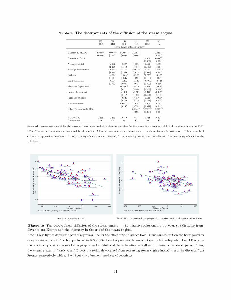
Indeed, in line with the historical account, the distribution of steam engines across French
departments, as reported in the 1860-1865 industrial survey, is indicative of a local diffusion process
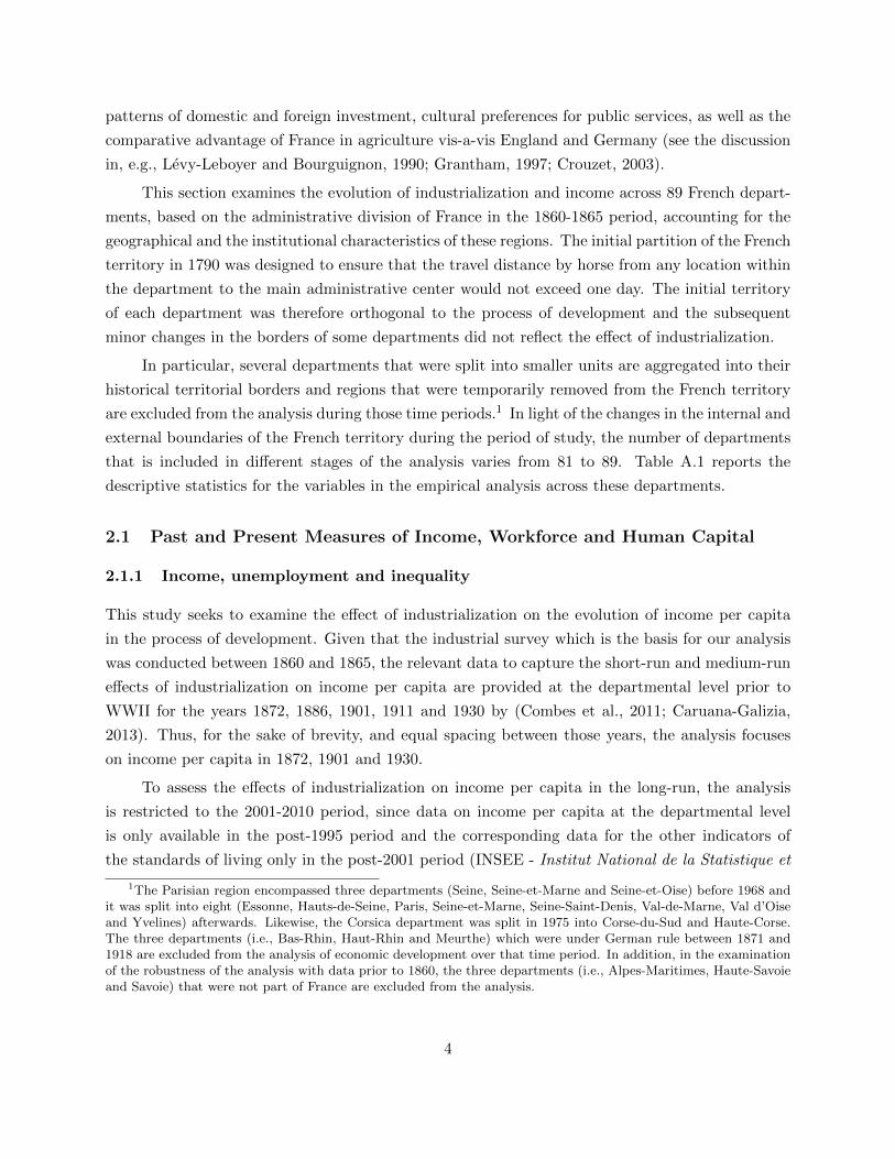
from Fresnes-sur-Escaut. As reported in Column 1 of Table 1 and shown in Panel A of Figure 3,
there is a highly significant negative correlation between the aerial distance from Fresnes-sur-Escaut
9There was also a regional pattern in the diffusion of steam engines in England (Kanefsky and Robey, 1980;Nuvolari et al., 2011) and in the USA (Atack, 1979).
10This steam engine was used to pump water in an ordinary mine of Fresnes-sur-Escaut. It is unclear whetherPierre Mathieu, the owner of the mine, built the engine himself after a trip in England or employed an Englishmanfor this purpose (Ballot, 1923, p.385).
10
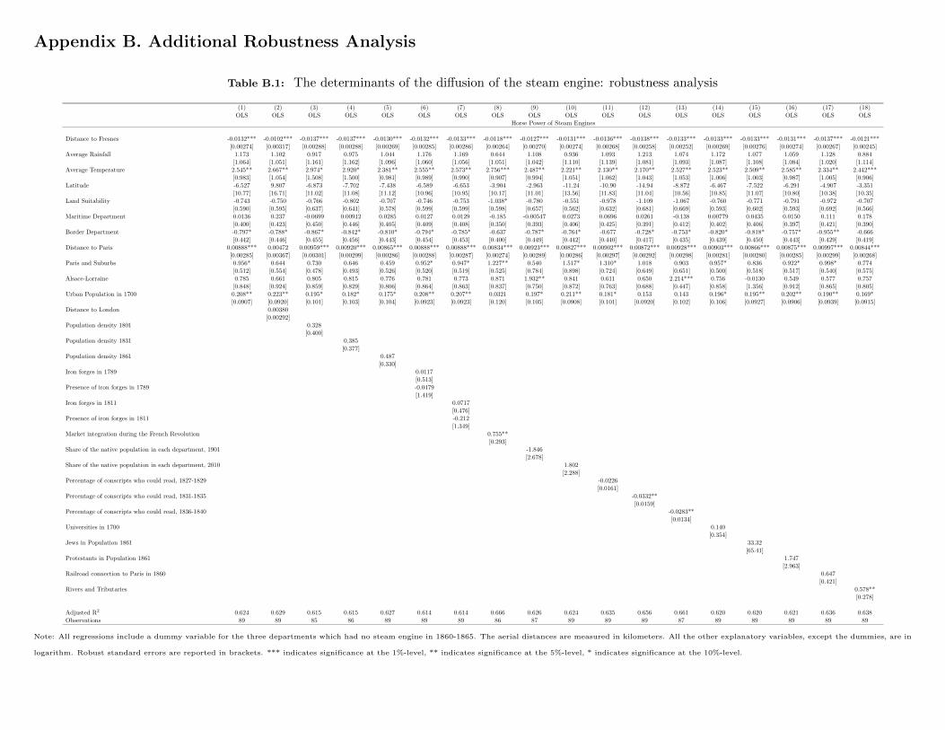
Table 1: The determinants of the diffusion of the steam engine
Note: All regressions, except for the unconditional ones, include a dummy variable for the three departments which had no steam engine in 1860-
1865. The aerial distances are measured in kilometers. All other explanatory variables except the dummies are in logarithm. Robust standard
errors are reported in brackets. *** indicates significance at the 1%-level, ** indicates significance at the 5%-level, * indicates significance at the
10%-level.
NORD
PAS-DE-CALAISAISNE
SOMMEARDENNES
OISE
MARNE
SEINE
SEINE-INFERIEURE
SEINE-ET-OISE
MEUSESEINE-ET-MARNE
EURE
MOSELLE
AUBEEURE-ET-LOIR
MEURTHE
HAUTE-MARNE
YONNELOIRET
CALVADOSVOSGES
ORNE
LOIR-ET-CHER
COTE-D'OR
BAS-RHIN
SARTHE
HAUTE-SAONE
MANCHE
HAUT-RHIN
CHER
NIEVRE
DOUBS
INDRE-ET-LOIRE
MAYENNE
INDRE
ALLIER
JURA
MAINE-ET-LOIRE
ILLE-ET-VILAINE
SAONE-ET-LOIRE
AIN
VIENNE
CREUSE
COTES-DU-NORD
LOIRE-INFERIEURE
PUY-DE-DOME
RHONE
HAUTE-SAVOIE
HAUTE-VIENNE
DEUX-SEVRES
MORBIHAN
VENDEE
LOIRE
SAVOIE
CHARENTE
CHARENTE-INFERIEURE
CORREZE
HAUTE-LOIRE
ISERE
CANTAL
DROME
FINISTERE
DORDOGNE
ARDECHE
LOZERE
HAUTES-ALPESLOT
AVEYRON
GIRONDE
VAUCLUSE
LOT-ET-GARONNE
TARN
BASSES-ALPES
TARN-ET-GARONNE
GARD
HERAULT
HAUTE-GARONNE
GERS
LANDESVAR (SAUF GRASSE 39-47)
ALPES MARITIMES (GRASSE 39-47)
BOUCHES-DU-RHONE
AUDE
HAUTES-PYRENEES
ARIEGE
BASSES-PYRENEES
PYRENEES-ORIENTALES
CORSE
-6-4
-20
24
Hor
se P
ower
of S
team
Eng
ines
(lo
g)
-400 -200 0 200 400 600Distance to Fresnes
coef = -.00523963, (robust) se = .00085142, t = -6.15
Panel A. Unconditional.
PAS-DE-CALAIS
NORD
ARDENNES
SOMME
AISNE
MARNE
LANDES
CORSE
VAR (SAUF GRASSE 39-47)
VOSGESHAUTE-MARNE
RHONE
DROME
HAUTE-SAONE
BOUCHES-DU-RHONE
LOIRE
GARD
AUDE
HERAULT
HAUTE-LOIRE
AIN
ARDECHE
LOZEREAUBE
SAONE-ET-LOIRE
SEINE-ET-MARNEYONNEMOSELLE
VAUCLUSE
CANTAL
ALLIER
OISE
CREUSE
PUY-DE-DOME
GERS
TARN
HAUT-RHIN
LOT
MEUSE
COTE-D'OR
NIEVRE
CORREZE
INDRE
DORDOGNE
PYRENEES-ORIENTALES
AVEYRON
HAUTES-ALPESISERE
GIRONDE
SEINE-ET-OISE
ARIEGE
MEURTHETARN-ET-GARONNE
LOT-ET-GARONNE
SEINE
CHER
BASSES-ALPES
EURE
VIENNE
CHARENTE
LOIR-ET-CHER
ALPES MARITIMES (GRASSE 39-47)
HAUTE-VIENNE
VENDEE
INDRE-ET-LOIRELOIRET
SEINE-INFERIEURE
EURE-ET-LOIR
CHARENTE-INFERIEURE
BAS-RHIN
SAVOIE
JURA
HAUTE-GARONNE
DEUX-SEVRES
HAUTES-PYRENEES
DOUBS
BASSES-PYRENEES
SARTHE
MANCHE
CALVADOS
MAINE-ET-LOIREHAUTE-SAVOIE
LOIRE-INFERIEURE
COTES-DU-NORD
ORNE
MAYENNE
MORBIHAN
ILLE-ET-VILAINEFINISTERE
-20
24
Hor
se P
ower
of S
team
Eng
ines
(lo
g)
-150 -100 -50 0 50 100Distance to Fresnes
coef = -.01320806, (robust) se = .00273856, t = -4.82
Panel B. Conditional on geography, institutions & distance from Paris.
Figure 3: The geographical diffusion of the steam engine − the negative relationship between the distance fromFresnes-sur-Escaut and the intensity in the use of the steam engine.
Note: These figures depict the partial regression line for the effect of the distance from Fresnes-sur-Escaut on the horse power in
steam engines in each French department in 1860-1865. Panel A presents the unconditional relationship while Panel B reports
the relationship which controls for geographic and institutional characteristics, as well as for pre-industrial development. Thus,
the x- and y-axes in Panels A and B plot the residuals obtained from regressing steam engine intensity and the distance from
Fresnes, respectively with and without the aforementioned set of covariates.
11
to the administrative center of each department and the intensity of the use of steam engines in
the department. Nevertheless, as discussed in Section 2.3, pre-industrial development and a wide
range of confounding geographical and institutional characteristics may have contributed to the
adoption of the steam engine. Reassuringly, the unconditional negative relationship remains highly
significant and is larger in absolute value when exogenous confounding geographical controls (i.e.,
land suitability, latitude, rainfall and temperature) (Column 2), as well as institutional factors
(Column 3) and pre-industrial development (Column 4), are accounted for. In particular, the
findings suggest that pre-industrial development, as captured by the degree of urbanization in
each department in 1700 and the characteristics that may have brought this early prosperity, had a
persistent positive and significant association with the adoption of the steam engine.11 Importantly,
the diffusion pattern of steam engines is not significantly correlated with the distance between
Paris and the administrative center of each department when the distance from Fresnes to each
department’s administrative center is excluded from the analysis (Column 5). Moreover, Column 6
of Table 1 and Panel B of Figure 3 indicate that there is still a highly significant negative correlation
between the distance from Fresnes-sur-Escaut to the administrative center of each department and
the intensity of the use of steam engines in the department when the distance to Paris is included. In
particular, a 100-km increase in the distance from Fresnes is associated with a 1.33 point decrease
in the log of the total horse power of the steam engines in a given department, relative to the
departmental average of log horse power of 3.26. Namely, if the distance of a department away
from Fresnes was to increase from the 25th percentile (336.6 km) to 75th percentile (680.3 km),
this department would experience a 4.57 point decrease in the log of the total horse power of steam
engines, i.e., a decrease in the amount of horse power worth 96.6 hp (relative to a sample mean of
655.24 hp).
The highly significant negative correlation between the use of the steam engine in each de-
partment and the aerial distance from Fresnes-sur-Escaut to the administrative center of each de-
partment is robust to the inclusion of an additional set of confounding geographical, demographic,
political and institutional characteristics, as well as to the forces of pre-industrial development,
which as discussed in section 4.2, may have contributed to the relationship between industrializa-
tion and economic development. As established in Table B.1 in Appendix B, these confounding
factors, which could be largely viewed as endogenous to the adoption of the steam engine and are
thus not part of the baseline analysis, do not affect the qualitative results.
The validity of the aerial distance from Fresnes-sur-Escaut as an instrumental variable for the
intensity of the adoption of steam engines across France is enhanced by third additional factors.
11Conceivably, human capital in the pre-industrial area could have affected the adoption of the steam engine, aswell as the subsequent process of development. Nevertheless, in light of the scarcity of data on reliable human capitalfor the pre-industrial period, the baseline analysis does not account for this confounding factor. Instead, Section4.2.3 shows the robustness of the results to the inclusion of pre-industrial levels of human capital for a smaller set ofdepartments.
12
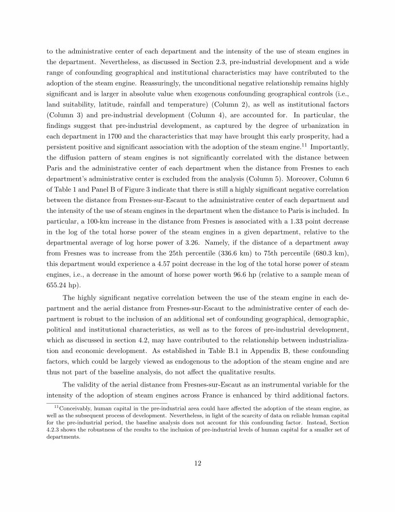
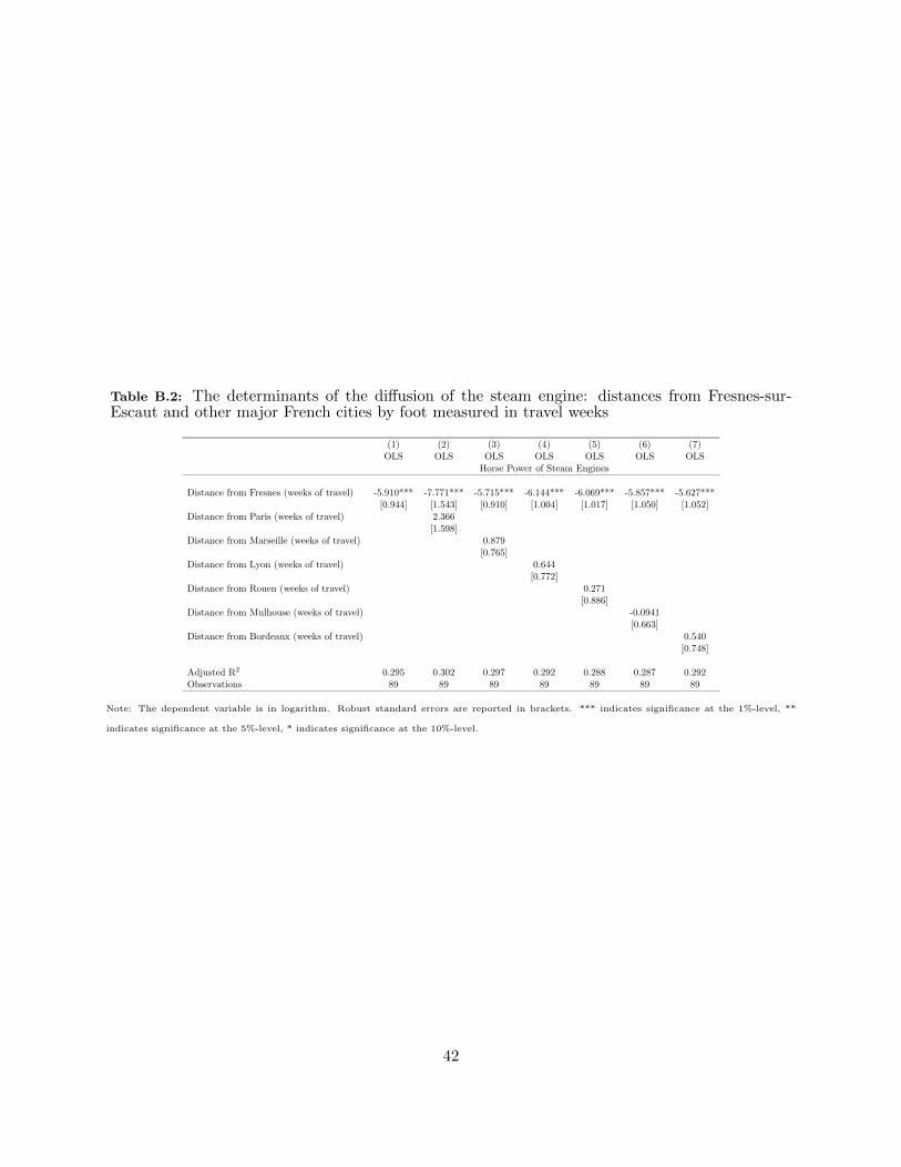
Table 2: The determinants of the diffusion of the steam engine: the insignificance of distancesfrom other major French cities
Note: Robust standard errors are reported in brackets. The dependent variable is in logarithm. The aerial distances are measured in kilometers.
*** indicates significance at the 1%-level, ** indicates significance at the 5%-level, * indicates significance at the 10%-level.
First, Table 2 establishes that, conditional on the distance from Fresnes-sur-Escaut, distances
between each department and major centers of economic power in 1860-1865 are uncorrelated with
the intensive use of the steam engine over this period. In particular, conditional on the distance
from Fresnes-sur-Escaut, distances between each department and Marseille and Lyon (the largest
cities in France), Rouen (a major harbor in the north-west where the steam engine was introduced
in 1796), Mulhouse (a major city in the east where the steam engine was introduced in 1812),
and Bordeaux (a major harbor in the south-west) are uncorrelated with the adoption of the steam
engine, lending credence to the unique role of Fresnes-sur-Escaut and the introduction of the first
steam engine in this location in the diffusion of the steam engine across France.12
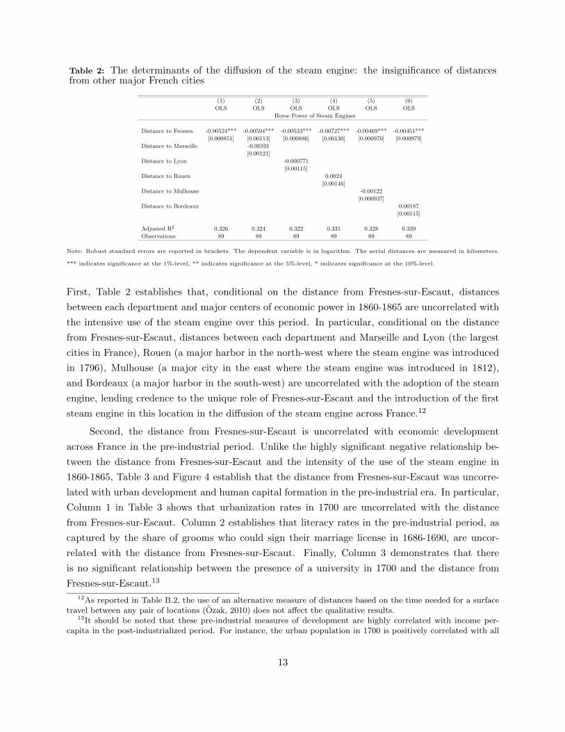
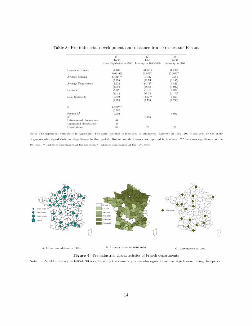
Second, the distance from Fresnes-sur-Escaut is uncorrelated with economic development
across France in the pre-industrial period. Unlike the highly significant negative relationship be-
tween the distance from Fresnes-sur-Escaut and the intensity of the use of the steam engine in
1860-1865, Table 3 and Figure 4 establish that the distance from Fresnes-sur-Escaut was uncorre-
lated with urban development and human capital formation in the pre-industrial era. In particular,
Column 1 in Table 3 shows that urbanization rates in 1700 are uncorrelated with the distance
from Fresnes-sur-Escaut. Column 2 establishes that literacy rates in the pre-industrial period, as
captured by the share of grooms who could sign their marriage license in 1686-1690, are uncor-
related with the distance from Fresnes-sur-Escaut. Finally, Column 3 demonstrates that there
is no significant relationship between the presence of a university in 1700 and the distance from
Fresnes-sur-Escaut.13
12As reported in Table B.2, the use of an alternative measure of distances based on the time needed for a surfacetravel between any pair of locations (Ozak, 2010) does not affect the qualitative results.
13It should be noted that these pre-industrial measures of development are highly correlated with income per-capita in the post-industrialized period. For instance, the urban population in 1700 is positively correlated with all
13
Table 3: Pre-industrial development and distance from Fresnes-sur-Escaut
(1) (2) (3)Tobit OLS Probit
Urban Population in 1700 Literacy in 1686-1690 University in 1700
Fresnes sur Escaut -0.004 -0.0219 0.0007[0.00499] [0.0232] [0.00267]
Average Rainfall -6.491*** -11.07 -1.564[2.455] [10.73] [1.155]
Average Temperature 3.722 -44.74** 0.827[3.094] [18.58] [1.902]
Latitude -9.320 -1.118 0.324[22.13] [85.55] [11.76]
Land Suitability 0.819 13.37** 0.863[1.474] [5.738] [0.756]
Note: The dependent variable is in logarithm. The aerial distance is measured in kilometers. Literacy in 1686-1690 is captured by the share
of grooms who signed their marriage license in that period. Robust standard errors are reported in brackets. *** indicates significance at the
1%-level, ** indicates significance at the 5%-level, * indicates significance at the 10%-level.
11000 - 15000
16000 - 55000
56000 - 134000
510000
A. Urban population in 1700.
No data
6.27 - 7.59
7.60 - 15.15
15.16 - 22.13
22.14 - 37.16
37.17 - 64.25
B. Literacy rates in 1686-1690.
University
C. Universities in 1700.
Figure 4: Pre-industrial characteristics of French departments
Note: In Panel B, literacy in 1686-1690 is captured by the share of grooms who signed their marriage license during that period.
14
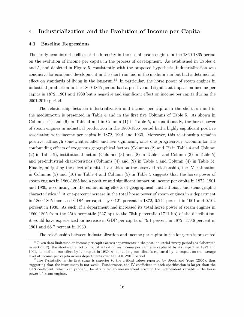
Third, it appears that the Nord department had neither superior human capital characteristics
nor higher standard of living in comparison to the average department in France. An imperfect
measure of literacy (i.e., men who could sign their wedding contract over the 1686-1690 period)
prior to the introduction of the first steam engine in 1732, suggests that if anything, Nord’s literacy
rate was below the French average. Specifically, only 10.45% of men in Nord could sign their
wedding contract over the 1686-1690 period while the average for the rest of France was 26.10%
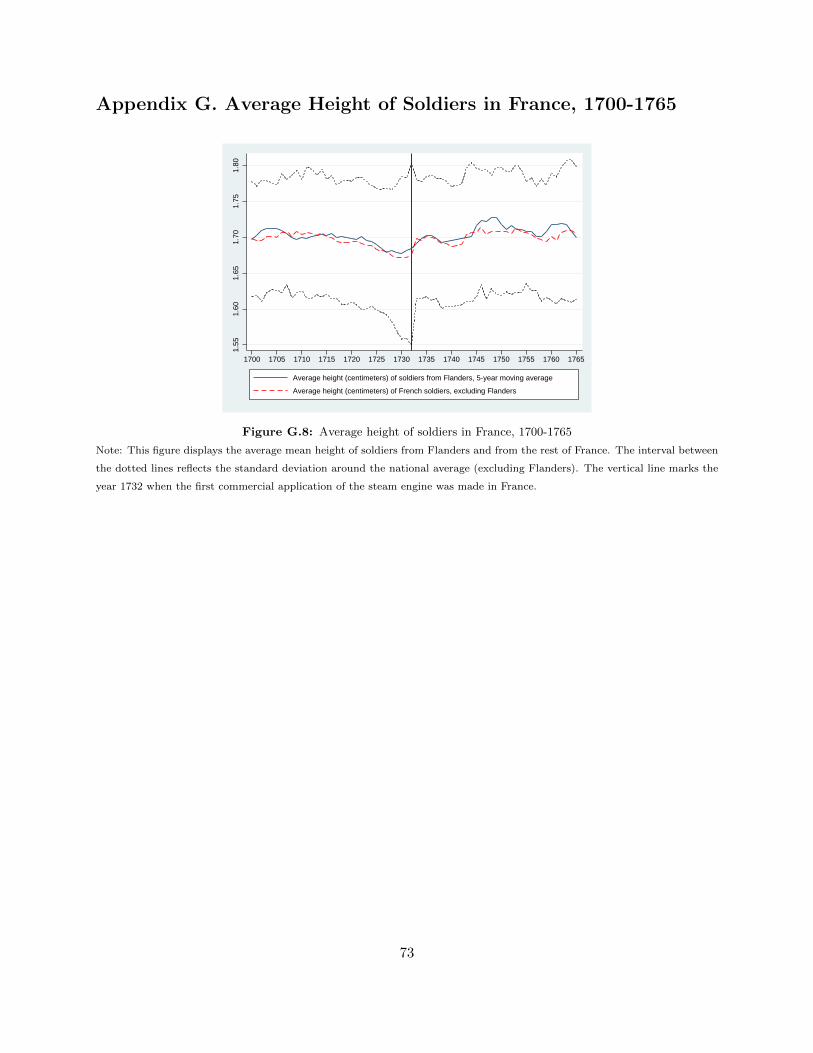
(with a standard deviation of 14.86%) (Furet and Ozouf, 1977). Furthermore, using height as an
indicator for the standard of living suggests that the standard living in Flanders, the province of
the French kingdom prior to 1789 which contained Fresnes-sur-Escaut, was nearly identical to that
of the rest of France (Komlos, 2005).14 As depicted in Figure G.8 in the Appendix, variations in
the average height of French army soldiers from Flanders over the 1700-65 period were not different
from those of the soldiers from other parts of France.
3.2 Empirical Model
The effect of industrialization on the process of development is estimated using 2SLS. The second
stage provides a cross-section estimate of the relationship between the total horse power of steam
engines in each department in 1860-1865 to measures of income per capita, human capital formation
and other economic outcomes at different points in time;
Yit = α+ βEi + X′iω + εit, (1)
where Yit represents one measure of economic outcomes in department i in year t, E i is the log of
total horse power of steam engines in department i in 1860-1865, X′i is a vector of geographical,
institutional and pre-industrial economic characteristics of department i and εit is an i.i.d. error
term for department i in year t.
In the first stage, E i, the log of total horse power of steam engines in department i in 1860-
1865 is instrumented by D i, the aerial distance (in kilometers) between the administrative center
of department i and Fresnes-sur-Escaut;
Ei = δ1Di + X′iδ2 + µi, (2)
where X′i is the same vector of geographical, institutional and pre-industrial economic characteris-
tics of department i used in the second stage, and µi is an error term for department i.
our measures of GDP per capita in 1872 (0.451), 1901 (0.293), 1930 (0.551) and 2001-2010 (0.517).14Concerns regarding selection bias suggest that the height of soldiers may not always be representative of the
height of the general population (see, e.g., Weir, 1997; Baten, 2000) but there is no reason to think that this selectionbias would be more or less intense in Flanders than in the rest of France.
15
4 Industrialization and the Evolution of Income per Capita
4.1 Baseline Regressions
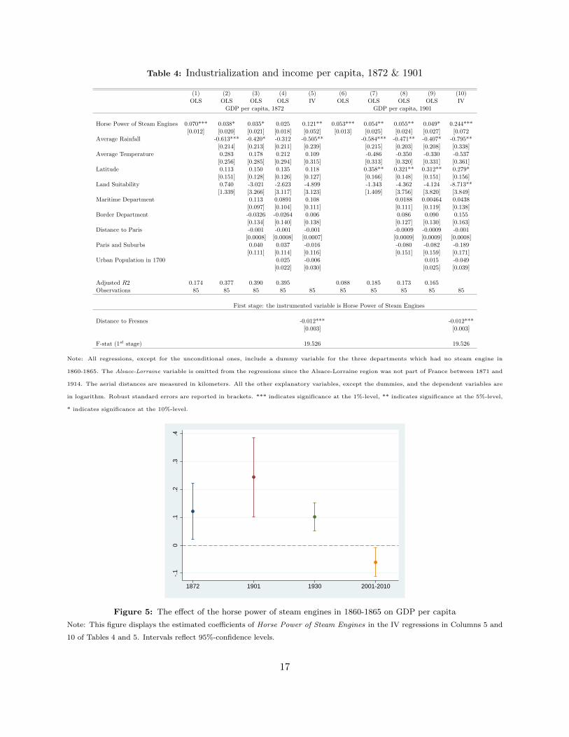
The study examines the effect of the intensity in the use of steam engines in the 1860-1865 period
on the evolution of income per capita in the process of development. As established in Tables 4
and 5, and depicted in Figure 5, consistently with the proposed hypothesis, industrialization was
conducive for economic development in the short-run and in the medium-run but had a detrimental
effect on standards of living in the long-run.15 In particular, the horse power of steam engines in
industrial production in the 1860-1865 period had a positive and significant impact on income per
capita in 1872, 1901 and 1930 but a negative and significant effect on income per capita during the
2001-2010 period.
The relationship between industrialization and income per capita in the short-run and in
the medium-run is presented in Table 4 and in the first five Columns of Table 5. As shown in
Columns (1) and (6) in Table 4 and in Column (1) in Table 5, unconditionally, the horse power
of steam engines in industrial production in the 1860-1865 period had a highly significant positive
association with income per capita in 1872, 1901 and 1930. Moreover, this relationship remains
positive, although somewhat smaller and less significant, once one progressively accounts for the
confounding effects of exogenous geographical factors (Columns (2) and (7) in Table 4 and Column
(2) in Table 5), institutional factors (Columns (3) and (8) in Table 4 and Column (3) in Table 5)
and pre-industrial characteristics (Columns (4) and (9) in Table 4 and Column (4) in Table 5).
Finally, mitigating the effect of omitted variables on the observed relationship, the IV estimation
in Columns (5) and (10) in Table 4 and Column (5) in Table 5 suggests that the horse power of
steam engines in 1860-1865 had a positive and significant impact on income per capita in 1872, 1901
and 1930, accounting for the confounding effects of geographical, institutional, and demographic
characteristics.16 A one-percent increase in the total horse power of steam engines in a department
in 1860-1865 increased GDP per capita by 0.121 percent in 1872, 0.244 percent in 1901 and 0.102
percent in 1930. As such, if a department had increased its total horse power of steam engines in
1860-1865 from the 25th percentile (227 hp) to the 75th percentile (1711 hp) of the distribution,
it would have experienced an increase in GDP per capita of 79.1 percent in 1872, 159.6 percent in
1901 and 66.7 percent in 1930.
The relationship between industrialization and income per capita in the long-run is presented
15Given data limitation on income per capita across departments in the post-industrial survey period (as elaboratedin section 2), the short-run effect of industrialization on income per capita is captured by its impact in 1872 and1901, its medium-run effect by its impact in 1930, while its long-run effect is captured by its impact on the averagelevel of income per capita across departments over the 2001-2010 period.
16The F-statistic in the first stage is superior to the critical values reported by Stock and Yogo (2005), thussuggesting that the instrument is not weak. Furthermore, the IV coefficient in each specification is larger than theOLS coefficient, which can probably be attributed to measurement error in the independent variable – the horsepower of steam engines.
16
Table 4: Industrialization and income per capita, 1872 & 1901
(1) (2) (3) (4) (5) (6) (7) (8) (9) (10)OLS OLS OLS OLS IV OLS OLS OLS OLS IV
lighting, furniture, clothing, food, transportation, sciences & arts, and luxury goods), the effect
of industrialization on income per capita in the process of development remains nearly intact,
economically and statistically.20
4.3 Industrialization, Employment and Inequality
This section explores the effect of industrialization on the evolution of sectoral employment from
1872 to 2010 and on contemporary levels of inequality.
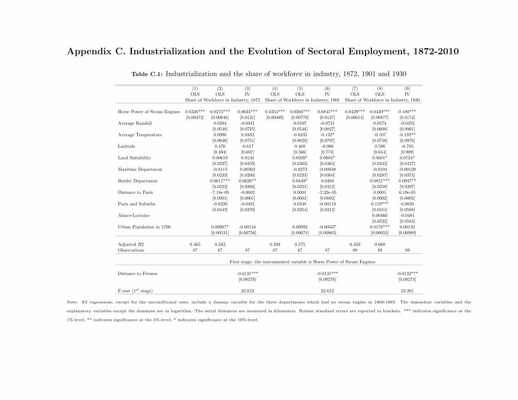
4.3.1 Industrialization and the Evolution of Sectoral Employment
The effect of the intensity in the use of the steam engine on the evolution of income per capita
corresponds to its effect on the share of employment in the industrial sector. As established in the
IV regressions in Columns (3), (6), and (9) of Table C.1 in Appendix C, and as depicted in panel
A of Figure 6, an intensive use of the steam engine in 1860-1865 had a highly significant positive
effect on the share of employment in the industrial sector in 1872, 1901, and 1930. Moreover, as
shown in the IV regressions in Column (3), (6), and (9) of Table C.2 in Appendix C, this effect
remains positive and highly significant in 1968, 1975, and 1982. However, as established in the IV
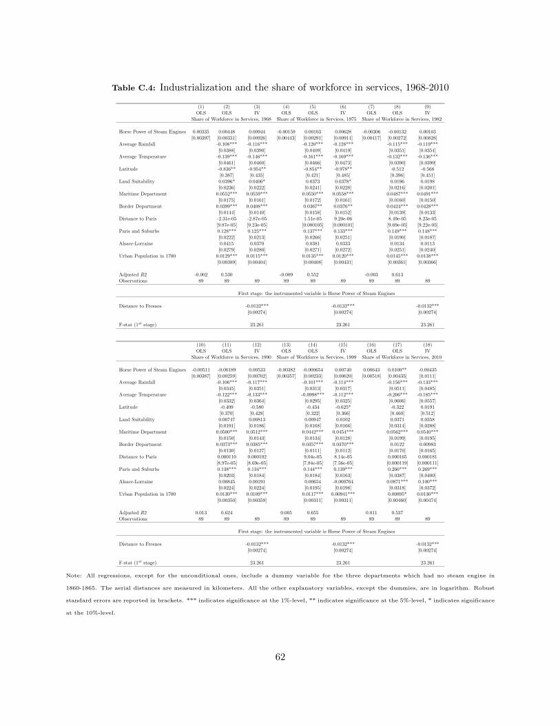
regressions in Column (12), (15), and (18) of Table C.2 in Appendix C, this effect dissipates in
1990 and 1999 and it becomes significantly negative in 2010. Furthermore, as established in the
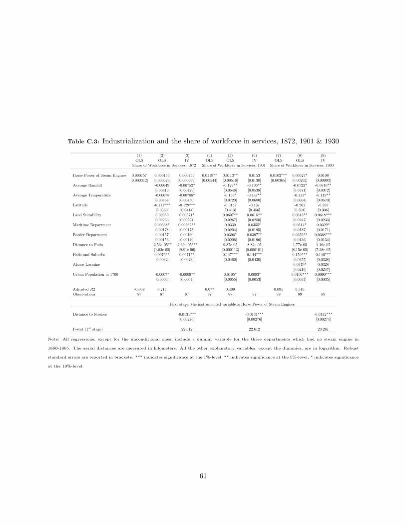
corresponding IV regressions in Tables C.3 and C.4 in Appendix C, and as depicted in panel B of
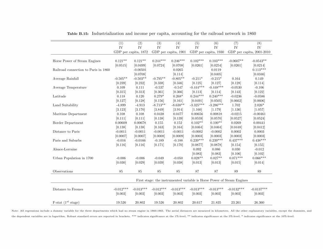
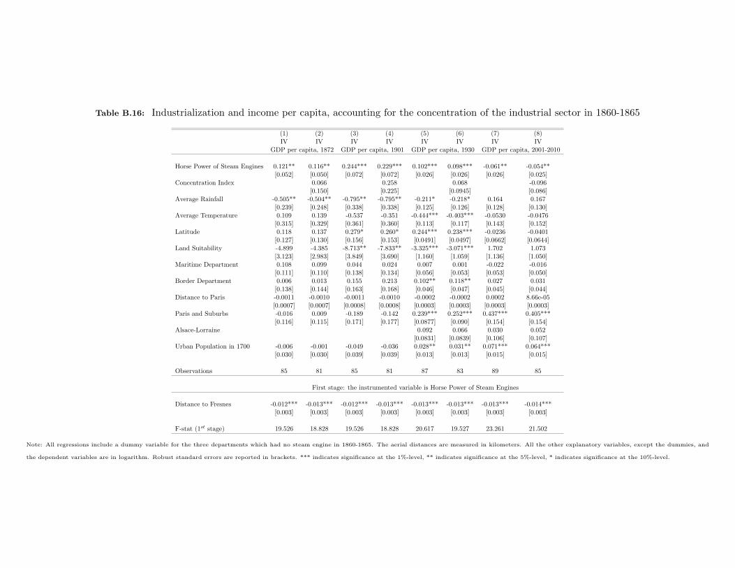
19The early network was built around seven lines in order to connect Paris to the main economic centres of thecountry (Caron, 1997).
20The Herfindahl index of industry concentration is defined as, Hd =∑16
i=1
(Ei,d/Ed
)2
, where H d is the Herfindahl
concentration index for department d, E i,d is the horse power of the steam engines in the firms in sector i of departmentd and Ed is the horse power of the steam engines in the firms of department d.
23
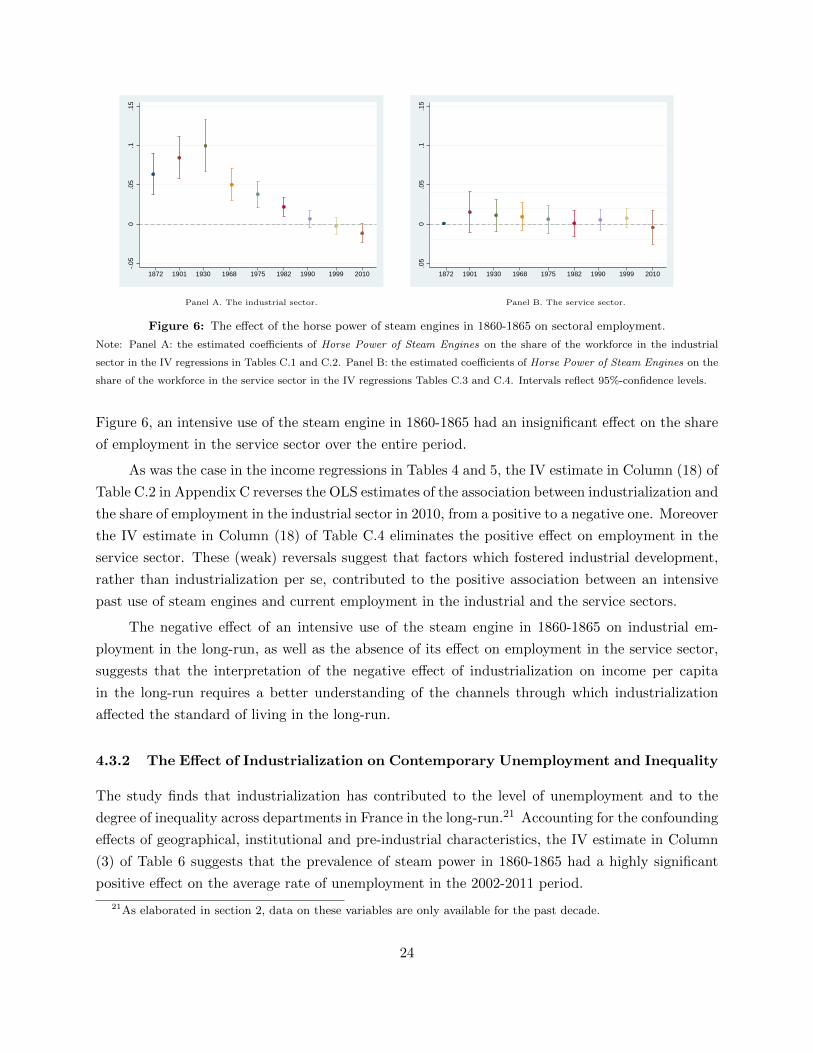
-.05
0.0
5.1
.15
19751901 1930 1968 1982 1990 1999 20101872
Panel A. The industrial sector.
0.0
5.0
5.1
5.1
19751872 1901 1930 1968 1982 1990 1999 2010
Panel B. The service sector.
Figure 6: The effect of the horse power of steam engines in 1860-1865 on sectoral employment.
Note: Panel A: the estimated coefficients of Horse Power of Steam Engines on the share of the workforce in the industrial
sector in the IV regressions in Tables C.1 and C.2. Panel B: the estimated coefficients of Horse Power of Steam Engines on the
share of the workforce in the service sector in the IV regressions Tables C.3 and C.4. Intervals reflect 95%-confidence levels.
Figure 6, an intensive use of the steam engine in 1860-1865 had an insignificant effect on the share
of employment in the service sector over the entire period.
As was the case in the income regressions in Tables 4 and 5, the IV estimate in Column (18) of
Table C.2 in Appendix C reverses the OLS estimates of the association between industrialization and
the share of employment in the industrial sector in 2010, from a positive to a negative one. Moreover
the IV estimate in Column (18) of Table C.4 eliminates the positive effect on employment in the
service sector. These (weak) reversals suggest that factors which fostered industrial development,
rather than industrialization per se, contributed to the positive association between an intensive
past use of steam engines and current employment in the industrial and the service sectors.
The negative effect of an intensive use of the steam engine in 1860-1865 on industrial em-
ployment in the long-run, as well as the absence of its effect on employment in the service sector,
suggests that the interpretation of the negative effect of industrialization on income per capita
in the long-run requires a better understanding of the channels through which industrialization
affected the standard of living in the long-run.
4.3.2 The Effect of Industrialization on Contemporary Unemployment and Inequality
The study finds that industrialization has contributed to the level of unemployment and to the
degree of inequality across departments in France in the long-run.21 Accounting for the confounding
effects of geographical, institutional and pre-industrial characteristics, the IV estimate in Column
(3) of Table 6 suggests that the prevalence of steam power in 1860-1865 had a highly significant
positive effect on the average rate of unemployment in the 2002-2011 period.
21As elaborated in section 2, data on these variables are only available for the past decade.
24
Table 6: Industrialization, unemployment and inequality
(1) (2) (3) (4) (5) (6) (7) (8) (9)OLS OLS IV OLS OLS IV OLS OLS IV
Unemployment rate Gini coefficient 25th Percentile - Fiscal Income per Person2002-2011 average 2001-2008 average in Household, 2001-2010 Average
First stage: the instrumented variable is Horse Power of Steam Engines
Distance to Fresnes -0.013*** -0.013*** -0.013***[0.003] [0.003] [0.003]
F-stat (1st stage) 23.261 23.261 23.261
Note: All regressions, except for the unconditional ones, include a dummy variable for the three departments which had no steam engine in 1860-
1865. The aerial distances are measured in kilometers. All the other explanatory variables, except the dummies, and the dependent variables are
in logarithm. Robust standard errors are reported in brackets. *** indicates significance at the 1%-level, ** indicates significance at the 5%-level,
* indicates significance at the 10%-level.
Moreover, as suggested by Column (6) of Table 6, the intensity in the use of steam engines in
1860-1865 had a positive and highly significant effect on the average Gini inequality index in the
2002-2011 period. Similarly, as reported in Column (9) of Table 6, it had a negative and highly
significant effect on the income of the individuals at the bottom 25th percentile of the income
distribution over the 2001-2010 period.
25
5 Mechanisms
This section explores potential mechanisms that could have led to the detrimental effect of indus-
trialization on the standard of living in the long-run. First, the study examines the adverse effect
of industrialization on the level and composition of human capital in each department and thus on
the skill-intensity of its production process in the long-run. Second, it explores the contribution
of industrialization to unionization and wage rates and thus the incentive of modern industries to
locate in regions where labor markets are more competitive and reflect the marginal productiv-
ity of workers. Third, the analysis examines the effect of on trade protection on the decline in
competitiveness of each department in the long-run.
5.1 Industrialization and the Long-Run Level Composition of Human Capital
This section explores whether the detrimental effect of industrialization on the standard of living in
the long-run could be attributed to the effect of industrialization on the evolution of human capital
formation. In particular, the study explores the potential adverse effect of industrialization on the
level and composition of human capital in each department and thus on the skill-intensity of its
production process in the long-run.
The analysis demonstrates that, while intensive industrialization had a significantly positive
effect on human capital formation in the short-run, it had a significantly negative effect in the level
and the composition of human capital in long-run.22 Hence, despite the fact that industrialization
had no effect on the share of employment in the service sector in the long-run, it had a detrimental
effect on skilled-intensive occupations. Thus, the adverse effect of industrialization on the level of
income per capita in the long-run could be partly attributed to the adverse effect of industrialization
on the level and the composition of human capital formation in the long-run.
5.1.1 Industrialization and the Evolution of Human Capital
This subsection examines the effect of industrialization on the time path of human capital formation.
As reported in Column (3) of Table 7, the horse power of steam engines in industrial production
in 1860-1865 had a highly significant positive effect on the literacy of the French army conscripts
in the years 1874-1883. However, due to the establishment of 1881-1882 education laws that made
primarily schooling compulsory and free till the age of 13, the effect is insignificant in the years
1894-1903 (Column (6)).
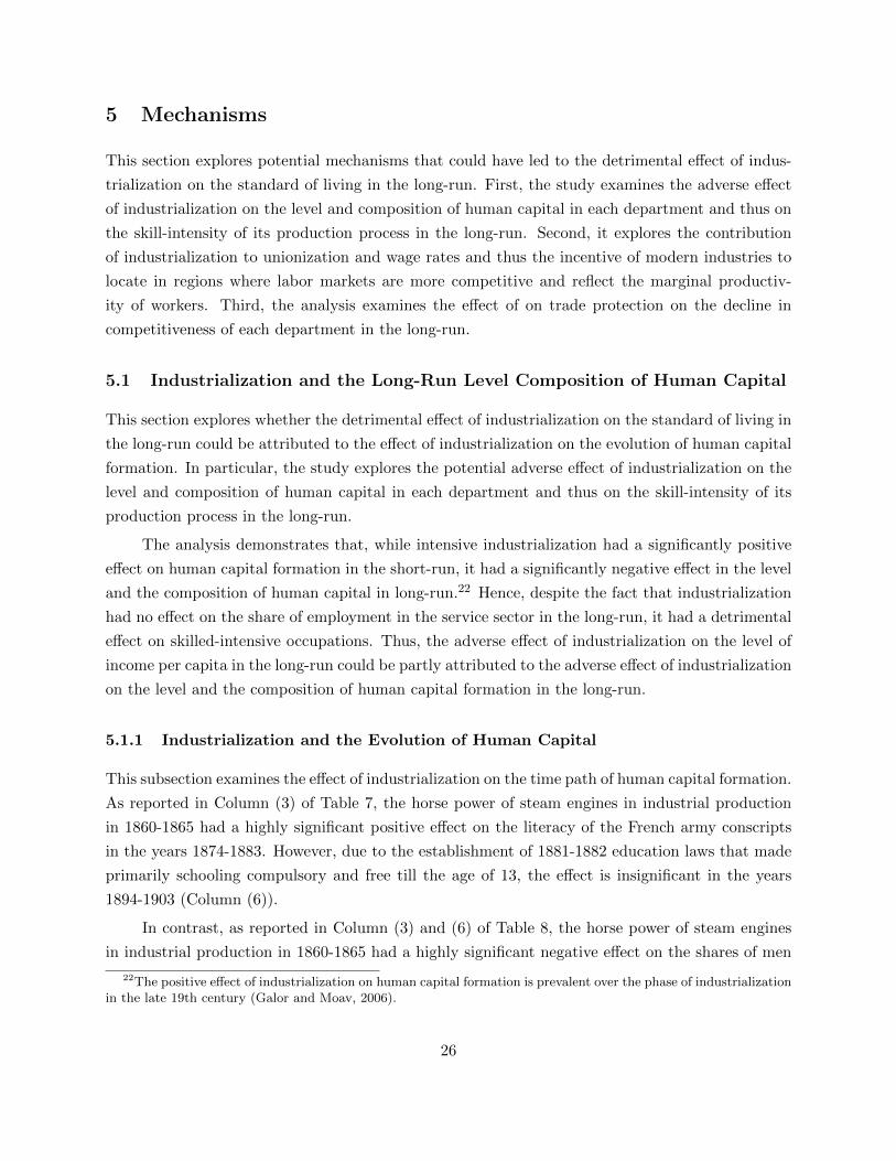
In contrast, as reported in Column (3) and (6) of Table 8, the horse power of steam engines
in industrial production in 1860-1865 had a highly significant negative effect on the shares of men
22The positive effect of industrialization on human capital formation is prevalent over the phase of industrializationin the late 19th century (Galor and Moav, 2006).
26
Table 7: Industrialization and the literacy of conscripts, 1874-1883 & 1894-1903
(1) (2) (3) (4) (5) (6)OLS OLS IV OLS OLS IV
Share of Literate Individuals Share of Literate IndividualsAmong Conscripts, 1874-1883 average Among Conscripts, 1894-1903 average
Horse Power of Steam Engines 0.008* 0.011 0.050*** 0.005** 0.008** 0.009[0.005] [0.008] [0.016] [0.002] [0.004] [0.006]
Average Rainfall 0.053 -0.013 -0.001 -0.004[0.074] [0.071] [0.033] [0.032]
Average Temperature -0.253*** -0.323*** -0.145*** -0.147***[0.079] [0.070] [0.030] [0.030]
Latitude -0.657 -1.815** -0.634** -0.680**[0.792] [0.768] [0.268] [0.290]
Land Suitability 0.153*** 0.161*** 0.069*** 0.069***[0.042] [0.041] [0.014] [0.013]
Maritime Department -0.037 -0.022 -0.012 -0.011[0.027] [0.029] [0.012] [0.011]
Border Department 0.044* 0.046 -0.001 -0.001[0.024] [0.030] [0.011] [0.010]
Distance to Paris -8.63e-05 -0.0002 -8.72e-05 -9.11e-05[0.0002] [0.0002] [6.96e-05] [6.55e-05]
Paris and Suburbs 0.0917*** 0.0630 0.0153 0.0142[0.034] [0.041] [0.013] [0.013]
Urban Population in 1700 0.004 -0.008 0.002 0.002[0.007] [0.009] [0.003] [0.003]
First stage: the instrumented variable is Horse Power of Steam Engines
Distance to Fresnes -0.013*** -0.013***[0.003] [0.003]
F-stat (1st stage) 23.261 23.261
Note: All regressions, except for the unconditional ones, include a dummy variable for the three departments which had no steam engine in
1860-1865. The aerial distances are measured in kilometers. All the other explanatory variables, except the dummies, are in logarithm. Robust
standard errors are reported in brackets. *** indicates significance at the 1%-level, ** indicates significance at the 5%-level, * indicates significance
at the 10%-level.
omitted factors, industrialization has an adverse effect on education in the long-run.
5.1.2 Industrialization in the Long-Run and the Composition of Human Capital
This subsection explores the effect of industrialization on the long-run composition of human cap-
ital as reflected by the share of executives, middle management professions, and employees (i.e.,
individuals with high, medium, and low levels of human capital) in the labor force. It demonstrates
that it had a detrimental effect on employment in skilled-intensive occupations, although industri-
alization had no effect on the share of employment in the service sector in the long-run (Panel B
of Figure 5).
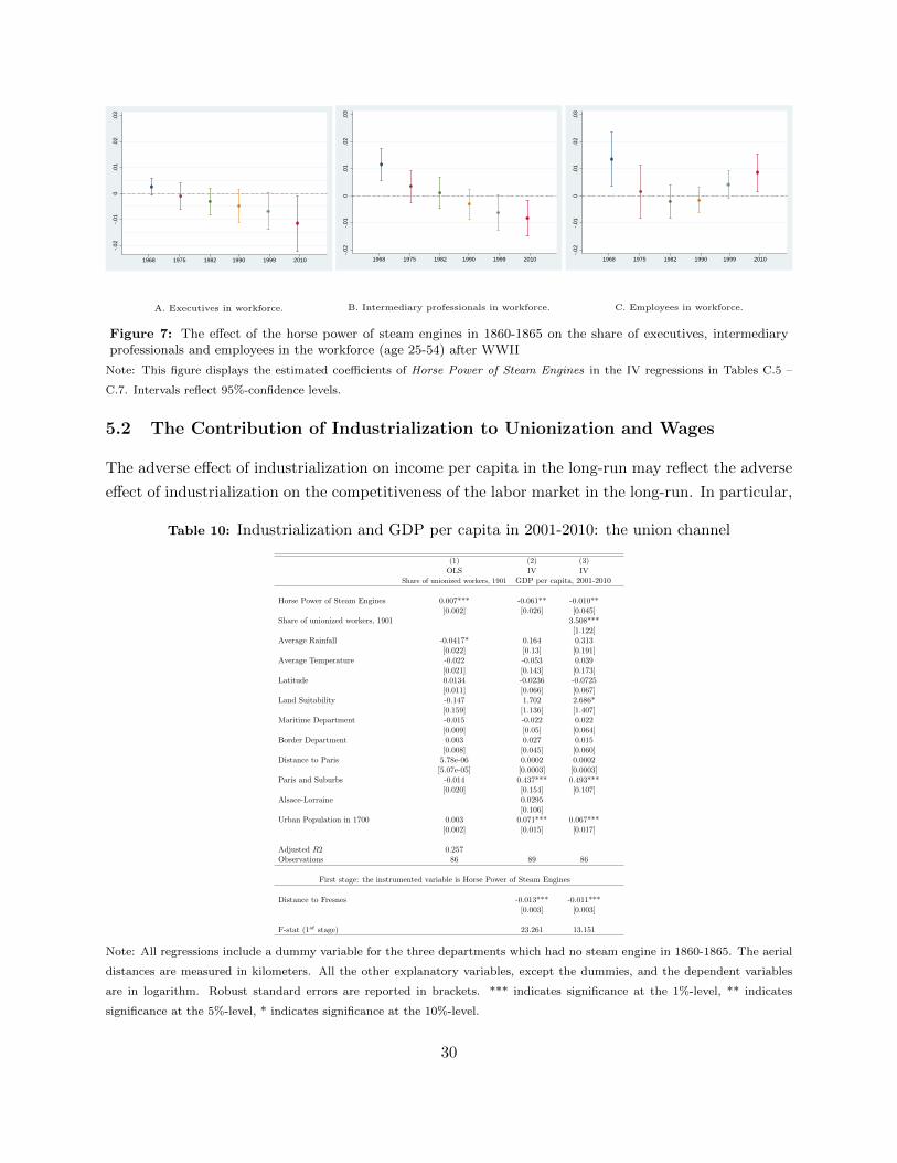
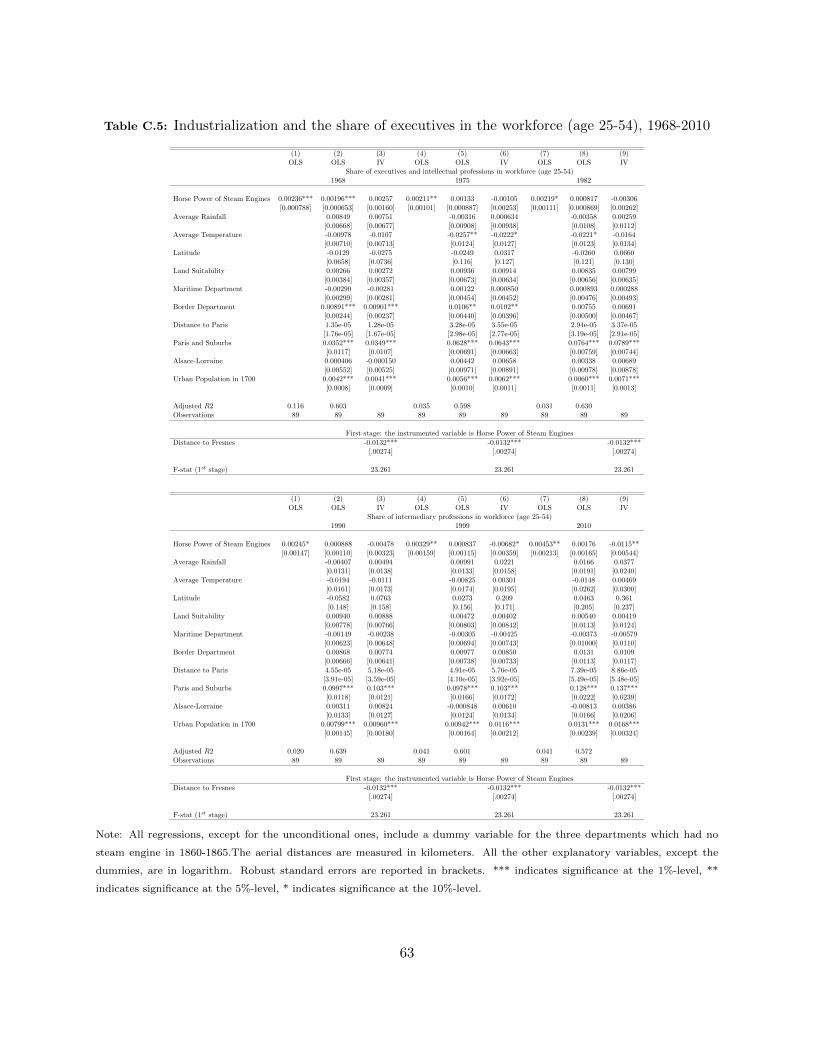
As depicted in Panels A–C of Figure 7 based on the IV regression in Tables C.5–C.7 in
Appendix C, the horse power of steam engines in industrial production in 1860-1865 had a significant
negative effect on the share of executives and other intellectual professions, as well as on the share
of middle management professions, among individuals age 25-54 in the years 1999 and 2010. In
contrast, the effect on the share of employees is significantly positive in 1999 and 2010.25
25The control group is made of farmers, artisans and other self-employed individuals.
28
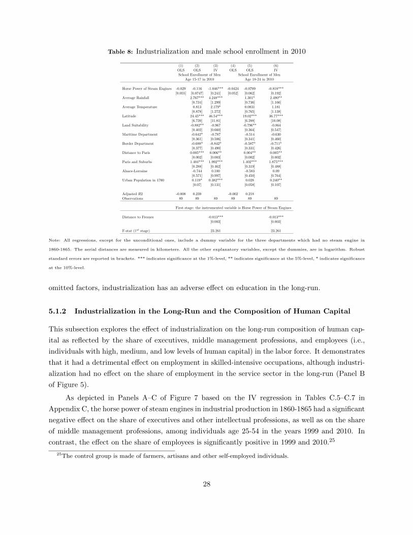
Table 9: Long-run effects of industrialization on human capital: male high-school and collegegraduates, 1968-2010
(1) (2) (3) (4) (5) (6) (7) (8) (9)OLS OLS IV OLS OLS IV OLS OLS IV
Share of Men Age 25 and above with Share of Men Age 25 and above with Share of Men Age 25 and above witha Secondary or Post-Secondary Degree, 1968 a Secondary or Post-Secondary Degree, 1975 a Secondary or Post-Secondary Degree, 1982
First stage: the instrumented variable is Horse Power of Steam Engines
Distance to Fresnes -0.013*** -0.013*** -0.013***[0.003] [0.003] [0.003]
F-stat (1st stage) 23.261 23.261 23.261
(10) (11) (12) (13) (14) (15) (16) (17) (18)OLS OLS IV OLS OLS IV OLS OLS IV
Share of Men Age 25 and above with Share of Men Age 25 and above with Share of Men Age 25 and above witha Secondary or Post-Secondary Degree, 1990 a Secondary or Post-Secondary Degree, 1999 a Secondary or Post-Secondary Degree, 2010
First stage: the instrumented variable is Horse Power of Steam Engines
Distance to Fresnes -0.013*** -0.013*** -0.013***[0.003] [0.003] [0.003]
F-stat (1st stage) 23.261 23.261 23.261
Note: All regressions, except for the unconditional ones, include a dummy variable for the three departments which had no steam engine in 1860-
1865. The aerial distances are measured in kilometers. All the other explanatory variables, except the dummies, and the dependent variables are
in logarithm. Robust standard errors are reported in brackets. *** indicates significance at the 1%-level, ** indicates significance at the 5%-level,
* indicates significance at the 10%-level.
29
-.02
-.01
0.0
1.0
2.0
3
1968 1975 1982 1990 20101999
A. Executives in workforce.
-.02
-.01
0.0
1.0
2.0
3
1968 1975 1982 1990 1999 2010
B. Intermediary professionals in workforce.
-.01
0.0
1.0
2.0
3-.
02
19751968 1982 1990 1999 2010
C. Employees in workforce.
Figure 7: The effect of the horse power of steam engines in 1860-1865 on the share of executives, intermediaryprofessionals and employees in the workforce (age 25-54) after WWII
Note: This figure displays the estimated coefficients of Horse Power of Steam Engines in the IV regressions in Tables C.5 –
C.7. Intervals reflect 95%-confidence levels.
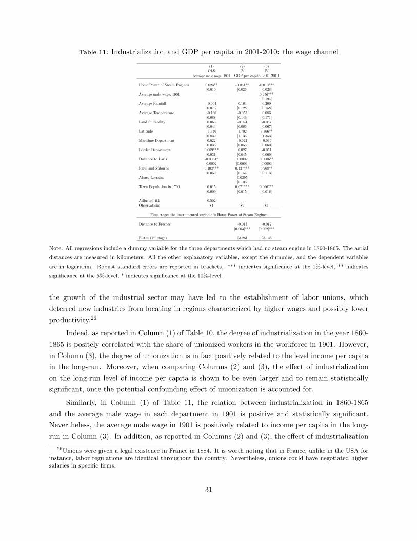
5.2 The Contribution of Industrialization to Unionization and Wages
The adverse effect of industrialization on income per capita in the long-run may reflect the adverse
effect of industrialization on the competitiveness of the labor market in the long-run. In particular,
Table 10: Industrialization and GDP per capita in 2001-2010: the union channel
(1) (2) (3)OLS IV IV
Share of unionized workers, 1901 GDP per capita, 2001-2010
Horse Power of Steam Engines 0.007*** -0.061** -0.010**[0.002] [0.026] [0.045]
Share of unionized workers, 1901 3.508***[1.122]
Average Rainfall -0.0417* 0.164 0.313[0.022] [0.13] [0.191]
Average Temperature -0.022 -0.053 0.039[0.021] [0.143] [0.173]
Latitude 0.0134 -0.0236 -0.0725[0.011] [0.066] [0.067]
Land Suitability -0.147 1.702 2.686*[0.159] [1.136] [1.407]
Maritime Department -0.015 -0.022 0.022[0.009] [0.05] [0.064]
Border Department 0.003 0.027 0.015[0.008] [0.045] [0.060]
Distance to Paris 5.78e-06 0.0002 0.0002[5.07e-05] [0.0003] [0.0003]
Paris and Suburbs -0.014 0.437*** 0.493***[0.020] [0.154] [0.107]
Alsace-Lorraine 0.0295[0.106]
Urban Population in 1700 0.003 0.071*** 0.067***[0.002] [0.015] [0.017]
Adjusted R2 0.257Observations 86 89 86
First stage: the instrumented variable is Horse Power of Steam Engines
Distance to Fresnes -0.013*** -0.011***[0.003] [0.003]
F-stat (1st stage) 23.261 13.151
Note: All regressions include a dummy variable for the three departments which had no steam engine in 1860-1865. The aerial
distances are measured in kilometers. All the other explanatory variables, except the dummies, and the dependent variables
are in logarithm. Robust standard errors are reported in brackets. *** indicates significance at the 1%-level, ** indicates
significance at the 5%-level, * indicates significance at the 10%-level.
30
Table 11: Industrialization and GDP per capita in 2001-2010: the wage channel
(1) (2) (3)OLS IV IV
Average male wage, 1901 GDP per capita, 2001-2010
Horse Power of Steam Engines 0.023** -0.061** -0.010***[0.010] [0.026] [0.028]
Average male wage, 1901 0.956***[0.194]
Average Rainfall -0.004 0.164 0.200[0.073] [0.128] [0.158]
Average Temperature -0.136 -0.053 0.083[0.088] [0.143] [0.171]
Land Suitability 0.063 -0.024 -0.057[0.044] [0.066] [0.067]
Latitude -1.346 1.702 3.366**[0.839] [1.136] [1.353]
Maritime Department 0.022 -0.022 -0.039[0.036] [0.053] [0.060]
Border Department 0.089*** 0.027 -0.051[0.031] [0.045] [0.060]
Distance to Paris -0.0004* 0.0002 0.0006**[0.0002] [0.0003] [0.0003]
Paris and Suburbs 0.193*** 0.437*** 0.268**[0.059] [0.154] [0.113]
Alsace-Lorraine 0.0295[0.106]
Town Population in 1700 0.015 0.071*** 0.066***[0.009] [0.015] [0.016]
Adjusted R2 0.502Observations 84 89 84
First stage: the instrumented variable is Horse Power of Steam Engines
Distance to Fresnes -0.013 -0.012[0.003]*** [0.002]***
F-stat (1st stage) 23.261 23.145
Note: All regressions include a dummy variable for the three departments which had no steam engine in 1860-1865. The aerial
distances are measured in kilometers. All the other explanatory variables, except the dummies, and the dependent variables
are in logarithm. Robust standard errors are reported in brackets. *** indicates significance at the 1%-level, ** indicates
significance at the 5%-level, * indicates significance at the 10%-level.
the growth of the industrial sector may have led to the establishment of labor unions, which
deterred new industries from locating in regions characterized by higher wages and possibly lower
productivity.26
Indeed, as reported in Column (1) of Table 10, the degree of industrialization in the year 1860-
1865 is positely correlated with the share of unionized workers in the workforce in 1901. However,
in Column (3), the degree of unionization is in fact positively related to the level income per capita
in the long-run. Moreover, when comparing Columns (2) and (3), the effect of industrialization
on the long-run level of income per capita is shown to be even larger and to remain statistically
significant, once the potential confounding effect of unionization is accounted for.
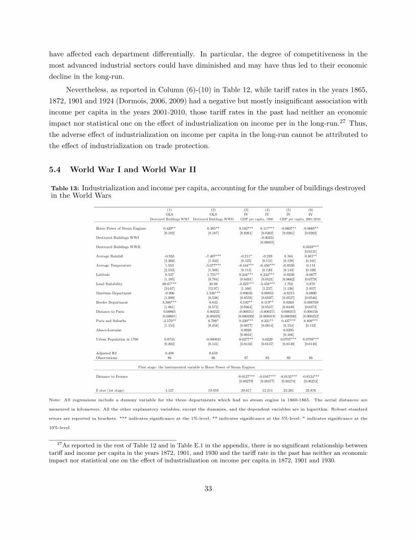
Similarly, in Column (1) of Table 11, the relation between industrialization in 1860-1865
and the average male wage in each department in 1901 is positive and statistically significant.
Nevertheless, the average male wage in 1901 is positively related to income per capita in the long-
run in Column (3). In addition, as reported in Columns (2) and (3), the effect of industrialization
26Unions were given a legal existence in France in 1884. It is worth noting that in France, unlike in the USA forinstance, labor regulations are identical throughout the country. Nevertheless, unions could have negotiated highersalaries in specific firms.
31
on the long-run level of income per capita is even larger and still significant statistically, once
the potential confounding effect of higher wages in the past is accounted for. Thus, the adverse
effect of industrialization on income per capita in the long-run cannot be attributed to the effect
of industrialization on unionization and wages.
5.3 Trade Protection and Competitiveness in the Long-Run
This section explores whether the detrimental effect of industrialization on the standard of living
in the long-run could be attributed to the adverse effect of trade protection on the competitiveness
of each department in the long-run.
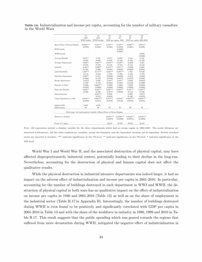
Table 12: Industrial and GDP per capita in 1930 & 2001-2010, acccounting for sectoral tariffprotection
(1) (2) (3) (4) (5) (6) (7) (8) (9) (10)IV IV IV IV IV IV IV IV IV IV
GDP per capita, 1930 GDP per capita, 2001-2010 average
Note: All regressions include a dummy variable for the three departments which had no steam engine in 1860-1865. The aerial distances are
measured in kilometers. All the other explanatory variables, except the dummies, and the dependent variables are in logarithm. Robust standard
errors are reported in brackets. *** indicates significance at the 1%-level, ** indicates significance at the 5%-level, * indicates significance at the
10%-level.
27As reported in the rest of Table 12 and in Table E.1 in the appendix, there is no significant relationship betweentariff and income per capita in the years 1872, 1901, and 1930 and the tariff rate in the past has neither an economicimpact nor statistical one on the effect of industrialization on income per capita in 1872, 1901 and 1930.
33
Table 14: Industrialization and income per capita, accounting for the number of military casualtiesin the World Wars
(1) (2) (3) (4) (5) (6)OLS OLS IV IV IV IV
WWI deaths WWII deaths GDP per capita, 1930 GDP per capita, 2001-2010
Horse Power of Steam Engines 0.0901*** 0.101*** 0.102*** 0.103*** -0.0607** -0.0571**[0.0250] [0.0321] [0.0261] [0.0258] [0.0261] [0.0255]
First stage: the instrumented variable is Horse Power of Steam Engines
Distance to Fresnes -0.0127*** -0.0128*** -0.0132*** -0.0135***[0.00279] [0.00293] [0.00274] [0.00280]
F-stat (1st stage) 20.617 19.105 23.261 23.457
Note: All regressions include a dummy variable for the three departments which had no steam engine in 1860-1865. The aerial distances are
measured in kilometers. All the other explanatory variables, except the dummies, and the dependent variables are in logarithm. Robust standard
errors are reported in brackets. *** indicates significance at the 1%-level, ** indicates significance at the 5%-level, * indicates significance at the
10%-level.
World War I and World War II, and the associated destruction of physical capital, may have
affected disproportionately industrial centers, potentially leading to their decline in the long-run.
Nevertheless, accounting for the destruction of physical and human capital does not affect the
qualitative results.
While the physical destruction in industrial intensive departments was indeed larger, it had no
impact on the adverse effect of industrialization and income per capita in 2001-2010. In particular,
accounting for the number of buildings destroyed in each department in WWI and WWII, the de-
struction of physical capital in both wars has no qualitative impact on the effect of industrialization
on income per capita in 1930 and 2001-2010 (Table 13) as well as on the share of employment in
the industrial sector (Table B.17 in Appendix B). Interestingly, the number of buildings destroyed
during WWII is even found to be positively and significantly correlated with GDP per capita in
2001-2010 in Table 13 and with the share of the workforce in industry in 1990, 1999 and 2010 in Ta-
ble B.17. This result suggests that the public spending which was geared towards the regions that
suffered from more devastation during WWII, mitigated the negative effect of industrialization in
34
the long-run. Similarly, the destruction of human capital (measured by the number of soldiers from
each department who died in each war) has no qualitative impact on the effect of industrialization
on income per capita in the long-run (Table 14) and on the share of employment in the industrial
sector (Table B.18 in Appendix B).
6 Concluding Remarks
This research explores the long-run effect of industrialization on the process of development. In
contrast to conventional wisdom that views industrial development as a catalyst for economic
growth, highlighting its persistent effect on economic prosperity, the study establishes that while
the adoption of industrial technology was initially conducive for economic development, it has had
a detrimental effect on standards of living in the long-run.
The study exploits exogenous source of regional variation in the adoption of steam engines dur-
ing the French industrial revolution to establish that regions which industrialized more intensively
experienced an increase in literacy rates more swiftly and generated higher income per capita in
the subsequent decades. Nevertheless, industrialization had an adverse effect on income per capita,
employment and equality by the turn of the 21st century.
The research explores potential mechanisms that could have led to the detrimental effect of
industrialization on the standard of living in the long-run. First, the study examines the adverse
effect of industrialization on the level and composition human capital and thus on the skill-intensity
of the production process in the long-run. Second, it explores the contribution of industrialization to
unionization and wage rates and thus the incentive of modern industries to locate in regions where
labor markets are more competitive. Third, the analysis examines the effect of on trade protection
on the decline in competitiveness of each department in the long-run. Fourth, it examines the effect
of intensive industrialization on destruction during WWI and WWII and its persistent effect on
economic development. The findings suggest that the adverse effect of industrialization on income
per capita in the long-run reflects neither greater unionization rates and higher wages nor trade
protection, but rather underinvestment in human capital, beyond basic literacy skills, and lower
employment in skilled-intensive occupations.
The study thus suggests that the characteristics that permitted the onset of industrialization,
rather than the adoption of industrial technology per se, have been the source of prosperity among
the currently developed economies that experienced an early industrialization.
35
References
Annuaire Statistique De La France (1878-1939), Imprimerie Nationale, Paris.
Atack, Jeremy (1979), ‘Fact in fiction? Relative in costs of steam and water power: a simulation approach’,
Explorations in Economic History 16(10), 409–437.
Ballot, Charles (1923), L’Introduction du Machinisme dans l’Industrie Francaise, Slatkine Reprints (1978),
Geneva.
Baten, Jorg (2000), ‘Heights and real wages in the 18th and 19th centuries: an international overview’,
Economic History Yearbook 41(41), 61–76.
Becker, Sascha O., Erik Hornung and Ludger Woessmann (2011), ‘Education and catch-up in the industrial
revolution’, American Economic Journal: Macroeconomics 3(3), 92–126.
Becker, Sascha O. and Ludger Woessmann (2009), ‘Was Weber wrong? a human capital theory of Protestant
economic history’, The Quarterly Journal of Economics 124(2), 531–596.
Bosker, Maarten, Eltjo Buringh and Jan Luiten van Zanden (2013), ‘From Baghdad to London: unravel-
ling urban development in Europe and the Arab world 800-1800’, Review of Economics and Statistics
95(4), 1418–1437.
Bresnahan, Timothy F. and Manuel Trajtenberg (1995), ‘General purpose technologies: engines of growth?’,
Journal of Econometrics 65(1), 83–108.
Cantoni, Davide (2015), ‘The economic effects of the Protestant Reformation: testing the Weber hypothesis
in the German lands’, Journal of the European Economic Association 13(0), 00–00.
Caron, Francois (1997), Histoire des chemins de fer en France: 1740-1883, Fayard, Paris.
Caruana-Galizia, Paul (2013), ‘Estimating French regional income: departmental per capita gross value
added, 1872-1911’, Research in Economic History 29, 71–95.
Chanut, Jean-Marie, Jean Heffer, Jacques Mairesse and Gilles Postel-Vinay (2000), LIndustrie Francaise au
Milieu du 19e Siecle. Les enquetes de la Statistique Generale de la France, EHESS, Paris.
Chemin, Matthieu and Etienne Wasmer (2009), ‘Using Alsace-Moselle local laws to build a difference-in-
differences estimation strategy of the employment effects of the 35-hour workweek regulation in france’,
Galor, Oded and Omer Moav (2006), ‘Das Human-Kapital: a theory of the demise of class structure’, Review
of Economic Studies 73, 85–117.
Grantham, George (1997), ‘The French cliometric revolution: a survey of cliometric contributions to French
economic history’, European Review of Economic History 1, 353–405.
Grew, Raymond and Patrick J. Harrigan (1991), School, State, and Society: The Growth of Elementary
Schooling in Nineteenth-Century France–A Quantitative Analysis, University of Michigan Press, Ann Ar-
bor, MI.
Jovanovic, Boyan and Peter L. Rousseau (2005), General purpose technologies, in P.Aghion and S.Durlauf,
eds, ‘Handbook of Economic Growth’, Elsevier North-Holland, Amsterdam, pp. 1181–1224.
Kanefsky, John and John Robey (1980), ‘Steam engines in 18th-century Britain: a quantitative assessment’,
Technology and Culture 21(2), 161–186.
Komlos, John (2005), ‘Height of French soldiers, 1716-1784’, ICPSR - Computer File 04363-v1.
Landes, David (1998), The Wealth and Poverty of Nations, Abacus, London.
Leon, Pierre (1976), L’affermissement du phenomene d’industrialisation, in F.Braudel and E.Labrousse, eds,
‘Histoire economique et sociale de la France, vol. 3’, PUF, Paris, pp. 475–616.
Lepetit, Bernard (1994), The Pre-Industrial Urban System: France, 1740-1840, Cambridge University Press,
Cambridge, UK.
Levy-Leboyer, Maurice and Francois Bourguignon (1990), The French Economy in the Nineteenth Century,
Cambridge University Press, Cambridge, UK.
Maddison, Angus (2001), The World Economy: A Millenium Perspective, OECD, Paris, France.
Michel, Edmond (1926), ‘La situation financiere et l’achevement de la reconstitution des regions devastees
au 31 decembre 1925’, Journal de la societe statistique de Paris 67, 248–277.
Michel, Edmond (1932), Les dommages de guerre de la France et leur reparation, Berger-Levrault, Paris,
France.
Mokyr, Joel (1990), The Lever of Riches, Oxford University Press, Oxford, U.K.
Nelson, Richard R. and Edmund S. Phelps (1966), ‘Heights and human welfare: Recent developments and
new directions’, American Economic Review 56(1-2), 69–75.
Nuvolari, Alessandro, Bart Verspagen and Nick von Tunzelmann (2011), ‘Steam engines in 18th-century
Britain: a quantitative assessment’, Cliometrica 21(5), 291–321.
Ozak, Omer (2010), The voyage of homo-oeconomicus: some economic measures of distance. Brown Univer-
sity Mimeo.
37
Ramankutty, Navin, Jonathan A. Foley, John Norman and Kevin McSweeney (2002), ‘The global distribu-
tion of cultivable lands: current patterns and sensitivity to possible climate change’, Global Ecology and
Biogeography 11(5), 377 392.
Rosenberg, Nathan and Manuel Trajtenberg (2004), ‘A general purpose technology at work: the Corliss
steam engine in the late nineteenth-century United States’, Journal of Economic History 64(1), 1–39.
See, Henri (1925), La vie economique de la France sous la Monarchie Censitaire (1815-1848), Librairie Felix
Alcan, Paris.
Stock, James H. and Motohiro Yogo (2005), Testing for weak instruments in linear IV regression, in J. H.Stock
and D. W.Andrews, eds, ‘Identification and Inference for Econometric Models: Essays in Honor of Thomas
J. Rothenberg’, Cambridge University Press, Cambridge UK, pp. 80–108.
Weber, Max (1930), The Protestant Ethic and the Spirit of Capitalism, Allen and Unwin, London, U.K.
Weir, David R. (1997), Health and welfare during industrialization, in R. H.Steckel and R.Floud, eds, ‘Health
and welfare during industrialization’, University of Chicago Press, Chicago, Ill., pp. 161–200.
Woronoff, Denis (1997), Les forges, 1811, in G.Beaur and P.Minard, eds, ‘Atlas de la revolution francaise:
Economie, Vol. 10’, Editions de l’ecole des hautes etudes en sciences sociales, Paris, pp. 99–100.
38
Online Appendix
Appendix A. Descriptive Statistics
Table A.1: Descriptive statistics
Obs Mean Std. Dev. Min MaxDependent VariablesIncomeGDP per capita, 1872 85 655.24 198.13 235.60 1197.00GDP per capita, 1901 85 862.91 270.96 255.30 1816.40GDP per capita, 1930 87 6464.61 1500.21 4033.47 14109.92GDP per capita, 2001-2011 average 89 23.39 4.71 17.87 56.00Unemployment, Gini Coefficient and 25th Percentile of the Income Distribution, Post 2000Unemployment rate, 2002-2011 average 89 8.38 1.58 5.05 12.59Gini coefficient, 2001-2008 average 89 0.36 0.02 0.33 0.441st Quartile Fiscal Income per Person in Household, 2001-2010 Average 89 7125.19 1411.45 5292.10 15686.58Workforce, Pre-WWIIShare of Workforce in Industry, 1872 87 0.21 0.10 0.05 0.49Share of Workforce in Industry, 1901 87 0.27 0.10 0.10 0.57Share of Workforce in Industry, 1930 89 0.33 0.13 0.12 0.66Share of Workforce in Services, 1872 87 0.01 0.01 0.00 0.03Share of Workforce in Services, 1901 87 0.24 0.08 0.12 0.53Share of Workforce in Services, 1930 89 0.21 0.06 0.12 0.47Workforce, Post-WWIIShare of Workforce in Industry, 1968 89 0.37 0.09 0.18 0.55Share of Workforce in Industry, 1975 89 0.36 0.08 0.18 0.55Share of Workforce in Industry, 1982 89 0.34 0.07 0.20 0.49Share of Workforce in Industry, 1990 89 0.31 0.06 0.15 0.44Share of Workforce in Industry, 1999 89 0.26 0.06 0.14 0.36Share of Workforce in Industry, 2010 89 0.23 0.03 0.14 0.33Share of Workforce in Services, 1968 89 0.40 0.07 0.28 0.60Share of Workforce in Services, 1975 89 0.46 0.07 0.33 0.65Share of Workforce in Services, 1982 89 0.53 0.07 0.40 0.71Share of Workforce in Services, 1990 89 0.60 0.07 0.47 0.76Share of Workforce in Services, 1999 89 0.68 0.06 0.57 0.85Share of Workforce in Services, 2010 89 0.53 0.09 0.37 0.86Share of Executives in Workforce (age 25-54), 1968 89 0.041 0.013 0.02 0.114Share of Executives in Workforce (age 25-54), 1975 89 0.066 0.02 0.034 0.143Share of Executives in Workforce (age 25-54), 1982 89 0.073 0.022 0.043 0.17Share of Executives in Workforce (age 25-54), 1990 89 0.093 0.028 0.059 0.229Share of Executives in Workforce (age 25-54), 1999 89 0.095 0.029 0.062 0.249Share of Executives in Workforce (age 25-54), 2010 89 0.114 0.04 0.07 0.319Share of Intermediary Professionals in Workforce (age 25-54), 1968 89 0.153 0.032 0.083 0.299Share of Intermediary Professionals in Workforce (age 25-54), 1975 89 0.218 0.034 0.147 0.315Share of Intermediary Professionals in Workforce (age 25-54), 1982 89 0.237 0.026 0.18 0.312Share of Intermediary Professionals in Workforce (age 25-54), 1990 89 0.263 0.022 0.224 0.321Share of Intermediary Professionals in Workforce (age 25-54), 1999 89 0.297 0.021 0.257 0.36Share of Intermediary Professionals in Workforce (age 25-54), 2010 89 0.283 0.022 0.244 0.369Share of Employees in Workforce (age 25-54), 1968 89 0.041 0.013 0.02 0.114Share of Employees in Workforce (age 25-54), 1975 89 0.066 0.02 0.034 0.143Share of Employees in Workforce (age 25-54), 1982 89 0.073 0.022 0.043 0.17Share of Employees in Workforce (age 25-54), 1990 89 0.093 0.028 0.059 0.229Share of Employees in Workforce (age 25-54), 1999 89 0.095 0.029 0.062 0.249Share of Employees in Workforce (age 25-54), 2010 89 0.114 0.04 0.07 0.319Education Measures, Pre-WWIAverage Share of Literate Individuals Among Conscripts, 1874-1883 Average 87 0.82 0.10 0.53 0.97Average Share of Literate Individuals Among Conscripts, 1894-1903 Average 87 0.94 0.04 0.82 0.99Education Measures, Post-WWIIShare of Men Age 25 and Above with a Secondary or Post-Secondary Degree, 1968 89 0.09 0.02 0.06 0.19Share of Men Age 25 and Above with a Secondary or Post-Secondary Degree, 1975 89 0.12 0.03 0.07 0.24Share of Men Age 25 and Above with a Secondary or Post-Secondary Degree, 1982 89 0.16 0.03 0.10 0.28Share of Men Age 25 and Above with a Secondary or Post-Secondary Degree, 1990 89 0.20 0.04 0.14 0.36Share of Men Age 25 and Above with a Secondary or Post-Secondary Degree, 1999 89 0.25 0.05 0.18 0.46Share of Men Age 25 and Above with a Secondary or Post-Secondary Degree, 2010 89 0.36 0.06 0.27 0.58Share of Women Age 25 and Above with a Secondary or Post-Secondary Degree, 1968 89 0.05 0.02 0.03 0.13Share of Women Age 25 and Above with a Secondary or Post-Secondary Degree, 1975 89 0.10 0.03 0.06 0.21Share of Women Age 25 and Above with a Secondary or Post-Secondary Degree, 1982 89 0.14 0.03 0.09 0.25Share of Women Age 25 and Above with a Secondary or Post-Secondary Degree, 1990 89 0.19 0.04 0.13 0.36Share of Women Age 25 and Above with a Secondary or Post-Secondary Degree, 1999 89 0.28 0.05 0.20 0.49Share of Women Age 25 and Above with a Secondary or Post-Secondary Degree, 2010 89 0.41 0.06 0.31 0.62School Enrollment of Men Age 15-17 in 2010 89 95.55 1.03 93.10 97.70School Enrollment of Women Age 15-17 in 2010 89 96.68 0.88 94.40 98.10School Enrollment of Men Age 18-24 in 2010 89 44.25 7.11 30.80 61.50School Enrollment of Women Age 18-24 in 2010 89 48.02 8.35 35.90 66.90Explanatory VariablesHorse Power of Steam Engines 89 1839.35 3855.33 0 27638Average Rainfall 89 878.03 156.42 642.90 1289.24Average Temperature 89 10.45 1.69 4.42 13.73Latitude 89 0.74 0.19 0.21 0.98Land Suitability 89 46.49 2.15 41.86 50.49Maritime Department 89 0.27 0.45 0 1Border Department 89 0.24 0.43 0 1Distance to Paris 89 365.88 188.95 1 918.86Paris and Suburbs 89 0.03 0.18 0 1Alsace-Lorraine 89 0.03 0.18 0 1Urban Population in 1700 (thousand of inhabitants) 89 20.79 57.78 0 510Instrumental VariableDistance to Fresnes sur Escaut 89 496.60 221.88 42.88 1027.22
Table A.2: Descriptive statistics: variables for robustness analysis.
Obs Mean Std. Dev. Min MaxEducation before 1840Grooms who Signed their Marriage License, 1686-1690 76 25.90 14.87 6.27 64.25Grooms who Signed their Marriage License, 1786-1790 79 42.35 23.94 5.24 92.18Grooms who Signed their Marriage License, 1816-1820 78 50.61 22.14 13.35 96.28Percentage of conscripts who could read, 1827-1829 89 15.11 14.90 0.90 61.70Percentage of conscripts who could read, 1831-1835 89 18.68 16.01 1.60 71.30Percentage of conscripts who could read, 1836-1840 87 23.90 17.50 1.50 77.70University 89 0.18 0.39 0 1Economic development before 1815Area covered by mines in department 89 0.008 0.015 0.00009 0.086Iron forges in 1789 89 2.15 8.76 0 52.00Iron forges in 1811 89 2.53 11.09 0 79.00Market integration during the French Revolution 86 132.71 106.95 21.00 732.00Presence of iron forges in 1789 89 0.10 0.30 0 1Presence of iron forges in 1811 89 0.10 0.30 0 1Railroad connectionRailroad connection to Paris in 1860 89 0.73 0.45 0 1Population densityPopulation density 1801 85 0.74 1.55 0.19 13.17Population density 1831 86 0.91 2.18 0.22 19.50Population density 1861 89 1.20 4.32 0.21 40.74Religious minoritiesJews in population, 1861 89 0.002 0.005 0 0.04Protestants in population, 1861 89 0.021 0.053 0.00003 0.31Horse Power of Steam Engines per inhabitant in 1861Horse Power of Steam Engines per inhabitant in 1861 89 0.003 0.005 0 0.03Share of the native populationShare of the native population in each department, 1901 87 0.85 0.09 0.47 0.98Share of the native population in each department, 2010 89 0.57 0.11 0.25 0.78World War I and World War IIDestroyed Buildings WWI 86 10802.81 38701.6 0 280175Destroyed Buildings WWII 86 13530.36 24260.73 0 122285WWI deaths 86 14677.21 10247.99 4226 80591WWII deaths 89 1568.236 1659.00 18 13218Access to WaterwaysRivers and Tributaries 89 0.562 0.499 0 1Distance from French cities - aerial distanceDistance from Marseille 89 472.93 215.91 1 902.67Distance from Lyon 89 330.99 152.35 1 723.27Distance from Rouen 89 420.42 210.31 1 1025.71Distance from Mulhouse 89 453.74 187.57 36.61 853.41Distance from Bordeaux 89 408.59 176.16 1 820.3Distance from French cities - weeks of travelDistance from Fresnes (weeks of travel) 89 0.480 0.187 0.045 0.895Distance from Paris (weeks of travel) 89 0.404 0.180 0.003 0.925Distance from Marseille (weeks of travel) 89 0.422 0.226 0.029 0.960Distance from Lyon (weeks of travel) 89 0.497 0.233 0.041 0.999Distance from Mulhouse (weeks of travel) 89 0.626 0.295 0.012 1.126Distance from Rouen (weeks of travel) 89 0.2 0.218 0.022 1.037Distance from Bordeaux (weeks of travel) 89 0.532 0.273 0.002 1.125Distance to LondonDistance to London (km) 89 636.23 229.93 242.93 1261.78Soldier deaths in World WarsSoldier deaths in World War I 89 14245.46 10339.62 893 80591Soldier deaths in World War II 89 1568.24 1659.00 18 13218Share of unionized workers in workforceShare of unionized workers in workforce, 1901 87 0.06 0.03 0.00 0.14Average wage, 1901 (in French Francs)Average male wage, 1901 84 4.23 0.73 2.66 7.61Concentration index, 1861Concentration index 85 0.40 0.20 0.12 1Weighted tariffs across sectorsWeighted tariffs across sectors, 1865 86 4.18 1.40 0.29 8.79Weighted tariffs across sectors, 1872 86 4.42 1.59 0.17 9.84Weighted tariffs across sectors, 1901 86 8.40 2.57 3.30 15.29Weighted tariffs across sectors, 1924 86 6.03 1.83 2.24 10.03
Appendix B. Additional Robustness Analysis
Table B.1: The determinants of the diffusion of the steam engine: robustness analysis
Note: All regressions include a dummy variable for the three departments which had no steam engine in 1860-1865. The aerial distances are measured in kilometers. All the other explanatory variables, except the dummies, are in
logarithm. Robust standard errors are reported in brackets. *** indicates significance at the 1%-level, ** indicates significance at the 5%-level, * indicates significance at the 10%-level.
Table B.2: The determinants of the diffusion of the steam engine: distances from Fresnes-sur-Escaut and other major French cities by foot measured in travel weeks
Note: All regressions include a dummy variable for the three departments which had no steam engine in 1860-1865. The aerial distances are measured in kilometers. All the other explanatory
variables, except the dummies, and the dependent variables are in logarithm. Robust standard errors are reported in brackets. *** indicates significance at the 1%-level, ** indicates significance
at the 5%-level, * indicates significance at the 10%-level.
Table B.4: Industrialization per capita in 1861 and the evolution of income per capita
(1) (2) (3) (4) (5) (6) (7) (8)IV IV IV IV IV IV IV IV
GDP per capita, 1872 GDP per capita, 1901 GDP per capita, 1930 GDP per capita, 2001-2010
Horse Power of Steam Engines 0.121** 0.244*** 0.102*** -0.061**[0.052] [0.072] [0.026] [0.026]
Horse Power of Steam Engines per inhabitant in 1861 31.67** 63.61*** 26.21*** -16.80**[14.78] [22.27] [8.140] [6.968]
Note: All regressions include a dummy variable for the three departments which had no steam engine in 1860-1865. The aerial distances are measured in kilometers. All the other explanatory variables, except the dummies, and
the dependent variables are in logarithm. Robust standard errors are reported in brackets. *** indicates significance at the 1%-level, ** indicates significance at the 5%-level, * indicates significance at the 10%-level.
Table B.5: Industrialization and income per capita, accounting for the distance to London
(1) (2) (3) (4) (5) (6) (7) (8)IV IV IV IV IV IV IV IV
GDP per capita, 1872 GDP per capita, 1901 GDP per capita, 1930 GDP per capita, 2001-2010
Horse Power of Steam Engines 0.121** 0.104 0.244*** 0.272** 0.102*** 0.120*** -0.0607** -0.111**[0.0515] [0.0714] [0.0724] [0.123] [0.0261] [0.0390] [0.0261] [0.0497]
Distance to London 0.000277 -0.000448 -0.000295 0.000844[0.000730] [0.00123] [0.000433] [0.000561]
Note: All regressions include a dummy variable for the three departments which had no steam engine in 1860-1865. The aerial distances are measured in kilometers. All the other explanatory variables, except the dummies, and
the dependent variables are in logarithm. Robust standard errors are reported in brackets. *** indicates significance at the 1%-level, ** indicates significance at the 5%-level, * indicates significance at the 10%-level.
Table B.6: Industrialization and income per capita, accounting for the presence of rivers and their main tributaries withindepartments
(1) (2) (3) (4) (5) (6) (7) (8)IV IV IV IV IV IV IV IV
GDP per capita, 1872 GDP per capita, 1901 GDP per capita, 1930 GDP per capita, 2001-2010
Horse Power of Steam Engines 0.121** 0.143** 0.244*** 0.268*** 0.102*** 0.0953*** -0.0607** -0.0761***[0.0515] [0.0612] [0.0724] [0.0795] [0.0261] [0.0276] [0.0261] [0.0270]
Rivers and Tributaries -0.125 -0.141 0.0387 0.103***[0.0849] [0.110] [0.0309] [0.0367]
Note: All regressions include a dummy variable for the three departments which had no steam engine in 1860-1865. The aerial distances are measured in kilometers. All the other explanatory
variables, except the dummies, and the dependent variables are in logarithm. Robust standard errors are reported in brackets. *** indicates significance at the 1%-level, ** indicates significance
at the 5%-level, * indicates significance at the 10%-level.
Table B.7: Industrialization and income per capita, accounting for the conscripts’ ability to read before 1840
(1) (2) (3) (4) (5) (6) (7) (8) (9) (10) (11) (12) (13) (14) (15) (16)IV IV IV IV IV IV IV IV IV IV IV IV IV IV IV IV
GDP per capita, 1872 GDP per capita, 1901 GDP per capita, 1930 GDP per capita, 2001-2010 average
Note: All regressions include a dummy variable for the three departments which had no steam engine in 1860-1865. The aerial distances are measured in kilometers. All the other explanatory variables, except the dummies, and
the dependent variables are in logarithm. Robust standard errors are reported in brackets. *** indicates significance at the 1%-level, ** indicates significance at the 5%-level, * indicates significance at the 10%-level.
Table B.8: Industrialization and income per capita, accounting for the share of grooms who signed their marriage license before 1820
(1) (2) (3) (4) (5) (6) (7) (8) (9) (10) (11) (12) (13) (14) (15) (16)IV IV IV IV IV IV IV IV IV IV IV IV IV IV IV IV
GDP per capita, 1872 GDP per capita, 1901 GDP per capita, 1930 GDP per capita, 2001-2010 average
Note: All regressions include a dummy variable for the three departments which had no steam engine in 1860-1865. The aerial distances are measured in kilometers. All the other explanatory variables, except the dummies, and
the dependent variables are in logarithm. Robust standard errors are reported in brackets. *** indicates significance at the 1%-level, ** indicates significance at the 5%-level, * indicates significance at the 10%-level.
Table B.9: Industrialization and income per capita, accounting for the number of universities in 1700
(1) (2) (3) (4) (5) (6) (7) (8)IV IV IV IV IV IV IV IV
GDP per capita, 1872 GDP per capita, 1901 GDP per capita, 1930 GDP per capita, 2001-2010
Horse Power of Steam Engine 0.121** 0.116** 0.244*** 0.244*** 0.102*** 0.106*** -0.0607** -0.0552**[0.0515] [0.0482] [0.0724] [0.0717] [0.0261] [0.0262] [0.0261] [0.0247]
University -0.0935 0.0106 0.0723* 0.0804**[0.0932] [0.121] [0.0405] [0.0378]
Note: All regressions include a dummy variable for the three departments which had no steam engine in 1860-1865. The aerial distances are measured in kilometers. All the other explanatory variables, except the dummies, and
the dependent variables are in logarithm. Robust standard errors are reported in brackets. *** indicates significance at the 1%-level, ** indicates significance at the 5%-level, * indicates significance at the 10%-level.
Table B.10: Industrialization and income per capita, accounting for religious minorities in 1861
(1) (2) (3) (4) (5) (6) (7) (8) (9) (10) (11) (12) (13) (14) (15) (16)IV IV IV IV IV IV IV IV IV IV IV IV IV IV IV IV
GDP per capita, 1872 GDP per capita, 1901 GDP per capita, 1930 GDP per capita, 2001-2010 average
Note: All regressions include a dummy variable for the three departments which had no steam engine in 1860-1865. The aerial distances are measured in kilometers. All the other explanatory variables, except the dummies, and
the dependent variables are in logarithm. Robust standard errors are reported in brackets. *** indicates significance at the 1%-level, ** indicates significance at the 5%-level, * indicates significance at the 10%-level.
Table B.11: Industrialization and income per capita, accounting for migrations
(1) (2) (3) (4)IV IV IV IV
GDP per capita, 1901 GDP per capita, 2001-2010
Horse Power of Steam Engines 0.121** 0.227*** -0.0607** -0.0598**[0.052] [0.070] [0.026] [0.026]
Share of the native population in each department, 1901 -1.530**[0.769]
Share of the native population in each department, 2010 -0.162[0.211]
Average Rainfall -0.505** -0.714** 0.164 0.185[0.239] [0.334] [0.128] [0.128]
Average Temperature 0.109 -0.484 -0.0530 -0.0262[0.315] [0.345] [0.143] [0.141]
Latitude 0.118 0.200 -0.0236 -0.0401[0.127] [0.162] [0.066] [0.063]
Land Suitability -4.899 -8.102** 1.702 2.131[3.123] [3.718] [1.136] [1.321]
Maritime Department 0.108 0.0981 -0.0215 -0.0227[0.111] [0.120] [0.0527] [0.0520]
Border Department 0.00609 0.144 0.0269 0.0246[0.138] [0.147] [0.0448] [0.0444]
Distance to Paris -0.001 -0.001 0.0002 0.0003[0.0007] [0.0008] [0.0003] [0.0003]
Paris and Suburbs -0.016 -0.539* 0.437*** 0.386**[0.116] [0.284] [0.154] [0.165]
Alsace-Lorraine 0.0295 0.0237[0.106] [0.105]
Urban Population in 1700 -0.006 -0.072* 0.071*** 0.070***[0.030] [0.038] [0.015] [0.015]
No Engine in 1860-1865 0.466* 0.925** -0.342*** -0.337***[0.249] [0.384] [0.125] [0.122]
Observations 85 85 89 89
First stage: the instrumented variable is Horse Power of Steam Engines
Distance to Fresnes -0.012*** -0.012*** -0.013*** -0.013***[0.003] [0.003] [0.003] [0.003]
F-stat (1st stage) 19.526 19.605 23.261 22.769
Note: Data on the native population in 1872 and 1930 are not available. All regressions, except for the unconditional ones, include a dummy variable for the three departments which had no steam engine in 1860-1865. The aerial
distances are measured in kilometers. All the other explanatory variables, except the dummies, and the dependent variables are in logarithm. Robust standard errors are reported in brackets. *** indicates significance at the
1%-level, ** indicates significance at the 5%-level, * indicates significance at the 10%-level.
Table B.12: Industrialization and income per capita, accounting for iron forges before 1811
(1) (2) (3) (4) (5) (6) (7) (8) (9) (10) (11) (12)IV IV IV IV IV IV IV IV IV IV IV IV
GDP per capita, 1872 GDP per capita, 1901 GDP per capita, 1930 GDP per capita, 2001-2010 average
Note: All regressions include a dummy variable for the three departments which had no steam engine in 1860-1865. The aerial distances are measured in kilometers. All the other explanatory variables, except the dummies, and
the dependent variables are in logarithm. Robust standard errors are reported in brackets. *** indicates significance at the 1%-level, ** indicates significance at the 5%-level, * indicates significance at the 10%-level.
Table B.13: Industrialization and income per capita, accounting for mines in 1837
(1) (2) (3) (4) (5) (6) (7) (8)IV IV IV IV IV IV IV IV
GDP per capita, 1872 GDP per capita, 1901 GDP per capita, 1930 GDP per capita, 2001-2010
Horse Power of Steam Engines 0.121** 0.164** 0.244*** 0.342*** 0.102*** 0.123*** -0.0607** -0.0708**[0.0515] [0.0803] [0.0724] [0.113] [0.0261] [0.0425] [0.0261] [0.0349]
Area Covered by Mines in Department -0.0374 -0.0852** -0.0193 0.0111[0.0281] [0.0397] [0.0169] [0.0124]
Note: All regressions include a dummy variable for the three departments which had no steam engine in 1860-1865. The aerial distances are
measured in kilometers. All the other explanatory variables, except the dummies, and the dependent variables are in logarithm. Robust standard
errors are reported in brackets. *** indicates significance at the 1%-level, ** indicates significance at the 5%-level, * indicates significance at the
10%-level.
Table B.14: Industrialization and income per capita, accounting for market integration during the French Revolution
(1) (2) (3) (4) (5) (6) (7) (8)IV IV IV IV IV IV IV IV
GDP per capita, 1872 GDP per capita, 1901 GDP per capita, 1930 GDP per capita, 2001-2010
Horse Power of Steam Engines 0.121** 0.113** 0.244*** 0.246*** 0.102*** 0.104*** -0.061** -0.078**[0.052] [0.057] [0.072] [0.073] [0.026] [0.027] [0.026] [0.031]
Market Integration during the French Revolution -0.050 -0.187* -0.046 0.127***[0.0921] [0.101] [0.0349] [0.0387]
Note: All regressions include a dummy variable for the three departments which had no steam engine in 1860-1865. The aerial distances are measured in kilometers. All the other explanatory
variables, except the dummies, and the dependent variables are in logarithm. Robust standard errors are reported in brackets. *** indicates significance at the 1%-level, ** indicates significance
at the 5%-level, * indicates significance at the 10%-level.
54
Table B.15: Industrialization and income per capita, accounting for the railroad network in 1860
(1) (2) (3) (4) (5) (6) (7) (8)IV IV IV IV IV IV IV IV
GDP per capita, 1872 GDP per capita, 1901 GDP per capita, 1930 GDP per capita, 2001-2010
Horse Power of Steam Engines 0.121** 0.121** 0.244*** 0.246*** 0.102*** 0.103*** -0.0607** -0.0543**[0.0515] [0.0499] [0.0724] [0.0708] [0.0261] [0.0254] [0.0261] [0.0214]
Railroad connection to Paris in 1860 -0.00501 0.0265 0.0119 0.113***[0.0708] [0.114] [0.0405] [0.0346]
Note: All regressions include a dummy variable for the three departments which had no steam engine in 1860-1865. The aerial distances are measured in kilometers. All the other explanatory variables, except the dummies, and
the dependent variables are in logarithm. Robust standard errors are reported in brackets. *** indicates significance at the 1%-level, ** indicates significance at the 5%-level, * indicates significance at the 10%-level.
Table B.16: Industrialization and income per capita, accounting for the concentration of the industrial sector in 1860-1865
(1) (2) (3) (4) (5) (6) (7) (8)IV IV IV IV IV IV IV IV
GDP per capita, 1872 GDP per capita, 1901 GDP per capita, 1930 GDP per capita, 2001-2010
Horse Power of Steam Engines 0.121** 0.116** 0.244*** 0.229*** 0.102*** 0.098*** -0.061** -0.054**[0.052] [0.050] [0.072] [0.072] [0.026] [0.026] [0.026] [0.025]
Concentration Index 0.066 0.258 0.068 -0.096[0.150] [0.225] [0.0945] [0.086]
Note: All regressions include a dummy variable for the three departments which had no steam engine in 1860-1865. The aerial distances are measured in kilometers. All the other explanatory variables, except the dummies, and
the dependent variables are in logarithm. Robust standard errors are reported in brackets. *** indicates significance at the 1%-level, ** indicates significance at the 5%-level, * indicates significance at the 10%-level.
Table B.17: Industrialization and the evolution of the share of the workforce in the industrial sector, accounting for the number of buildings destroyed inthe World Wars
(1) (2) (3) (4) (5) (6) (7) (8) (9) (10) (11) (12) (13) (14)IV IV IV IV IV IV IV IV IV IV IV IV IV IV
Share of Workforce in Industry Share of Workforce in Industry Share of Workforce in Industry Share of Workforce in Industry Share of Workforce in Industry Share of Workforce in Industry Share of Workforce in Industry1930 1968 1975 1982 1990 1999 2010
Note: All regressions include a dummy variable for the three departments which had no steam engine in 1860-1865. The aerial distances are measured in kilometers. All the other explanatory variables, except the dummies, and
the dependent variables are in logarithm. Robust standard errors are reported in brackets. *** indicates significance at the 1%-level, ** indicates significance at the 5%-level, * indicates significance at the 10%-level.
Table B.18: Industrialization and the evolution of the share of the workforce in the industrial sector, accounting for military casualties in the World Wars
(1) (2) (3) (4) (5) (6) (7) (8) (9) (10) (11) (12) (13) (14)IV IV IV IV IV IV IV IV IV IV IV IV IV IV
Share of Workforce in Industry Share of Workforce in Industry Share of Workforce in Industry Share of Workforce in Industry Share of Workforce in Industry Share of Workforce in Industry Share of Workforce in Industry1930 1968 1975 1982 1990 1999 2010
Note: All regressions include a dummy variable for the three departments which had no steam engine in 1860-1865. The aerial distances are measured in kilometers. All the other explanatory variables, except the dummies, and
the dependent variables are in logarithm. Robust standard errors are reported in brackets. *** indicates significance at the 1%-level, ** indicates significance at the 5%-level, * indicates significance at the 10%-level.
Appendix C. Industrialization and the Evolution of Sectoral Employment, 1872-2010
Table C.1: Industrialization and the share of workforce in industry, 1872, 1901 and 1930
(1) (2) (3) (4) (5) (6) (7) (8) (9)OLS OLS IV OLS OLS IV OLS OLS IV
Share of Workforce in Industry, 1872 Share of Workforce in Industry, 1901 Share of Workforce in Industry, 1930
First stage: the instrumented variable is Horse Power of Steam Engines
Distance to Fresnes -0.0131*** -0.0131*** -0.0132***[0.00276] [0.00276] [0.00274]
F-stat (1st stage) 22.612 22.612 23.261
Note: All regressions, except for the unconditional ones, include a dummy variable for the three departments which had no steam engine in 1860-1865. The dependent variables and the
explanatory variables except the dummies are in logarithm. The aerial distances are measured in kilometers. Robust standard errors are reported in brackets. *** indicates significance at the
1%-level, ** indicates significance at the 5%-level, * indicates significance at the 10%-level.
Table C.2: Industrialization and the share of workforce in industry, 1968-2010
(1) (2) (3) (4) (5) (6) (7) (8) (9)OLS OLS IV OLS OLS IV OLS OLS IV
Share of Workforce in Industry, 1968 Share of Workforce in Industry, 1975 Share of Workforce in Industry, 1982
First stage: the instrumented variable is Horse Power of Steam Engines
Distance to Fresnes -0.0132*** -0.0132*** -0.0132***[0.00274] [0.00274] [0.00274]
F-stat (1st stage) 23.261 23.261 23.261
Note: All regressions, except for the unconditional ones, include a dummy variable for the three departments which had no steam engine in
1860-1865. The aerial distances are measured in kilometers. All the other explanatory variables, except the dummies, are in logarithm. Robust
standard errors are reported in brackets. *** indicates significance at the 1%-level, ** indicates significance at the 5%-level, * indicates significance
at the 10%-level.
60
Table C.3: Industrialization and the share of workforce in services, 1872, 1901 & 1930
(1) (2) (3) (4) (5) (6) (7) (8) (9)OLS OLS IV OLS OLS IV OLS OLS IV
Share of Workforce in Services, 1872 Share of Workforce in Services, 1901 Share of Workforce in Services, 1930
First stage: the instrumented variable is Horse Power of Steam Engines
Distance to Fresnes -0.0131*** -0.0131*** -0.0132***[0.00276] [0.00276] [0.00274]
F-stat (1st stage) 22.612 22.612 23.261
Note: All regressions, except for the unconditional ones, include a dummy variable for the three departments which had no steam engine in
1860-1865. The aerial distances are measured in kilometers. All the other explanatory variables, except the dummies, are in logarithm. Robust
standard errors are reported in brackets. *** indicates significance at the 1%-level, ** indicates significance at the 5%-level, * indicates significance
at the 10%-level.
61
Table C.4: Industrialization and the share of workforce in services, 1968-2010
(1) (2) (3) (4) (5) (6) (7) (8) (9)OLS OLS IV OLS OLS IV OLS OLS IV
Share of Workforce in Services, 1968 Share of Workforce in Services, 1975 Share of Workforce in Services, 1982
First stage: the instrumented variable is Horse Power of Steam Engines
Distance to Fresnes -0.0132*** -0.0132*** -0.0132***[0.00274] [0.00274] [0.00274]
F-stat (1st stage) 23.261 23.261 23.261
Note: All regressions, except for the unconditional ones, include a dummy variable for the three departments which had no steam engine in
1860-1865. The aerial distances are measured in kilometers. All the other explanatory variables, except the dummies, are in logarithm. Robust
standard errors are reported in brackets. *** indicates significance at the 1%-level, ** indicates significance at the 5%-level, * indicates significance
at the 10%-level.
62
Table C.5: Industrialization and the share of executives in the workforce (age 25-54), 1968-2010
(1) (2) (3) (4) (5) (6) (7) (8) (9)OLS OLS IV OLS OLS IV OLS OLS IV
Share of executives and intellectual professions in workforce (age 25-54)1968 1975 1982
First stage: the instrumented variable is Horse Power of Steam Engines
Distance to Fresnes -0.0132*** -0.0132***[0.00274] [0.00274]
F-stat (1st stage) 23.261 23.261
Note: All regressions, except for the unconditional ones, include a dummy variable for the three departments which had no steam engine in 1860-1865. The
aerial distances are measured in kilometers. All the other explanatory variables, except the dummies, are in logarithm. Robust standard errors are reported
in brackets. *** indicates significance at the 1%-level, ** indicates significance at the 5%-level, * indicates significance at the 10%-level.
66
Table D.2: The long-run effects of industrialization on human capital: female high-school and college graduates,1968-2010
(1) (2) (3) (4) (5) (6) (7) (8) (9)OLS OLS IV OLS OLS IV OLS OLS IVShare of Women Age 25 and above with Share of Women Age 25 and above with Share of Women Age 25 and above with
a Secondary or Post-Secondary Degree, 1968 a Secondary or Post-Secondary Degree, 1975 a Secondary or Post-Secondary Degree, 1982
First stage: the instrumented variable is Horse Power of Steam Engines
Distance to Fresnes -0.0132*** -0.0132*** -0.0132***[0.00274] [0.00274] [0.00274]
F-stat (1st stage) 23.261 23.261 23.261
(10) (11) (12) (13) (14) (15) (16) (17) (18)OLS OLS IV OLS OLS IV OLS OLS IVShare of Women Age 25 and above with Share of Women Age 25 and above with Share of Women Age 25 and above with
a Secondary or Post-Secondary Degree, 1990 a Secondary or Post-Secondary Degree, 1999 a Secondary or Post-Secondary Degree, 2010
First stage: the instrumented variable is Horse Power of Steam Engines
Distance to Fresnes -0.0132*** -0.0132*** -0.0132***[0.00274] [0.00274] [0.00274]
F-stat (1st stage) 23.261 23.261 23.261
Note: All regressions, except for the unconditional ones, include a dummy variable for the three departments which had no steam engine in 1860-1865. The aerial distances are
measured in kilometers. All the other explanatory variables, except the dummies, are in logarithm. Robust standard errors are reported in brackets. *** indicates significance
at the 1%-level, ** indicates significance at the 5%-level, * indicates significance at the 10%-level.
Appendix E. Industrialization and GDP per Capita, 1872 & 1901,
Accounting for Sectoral Tariff Protection
Table E.1: Industrialization and income per capita, 1872 & 1901, accounting for sectoral tariffprotection
(1) (2) (3) (4) (5) (6) (7)IV IV IV IV IV IV IV
GDP per capita, 1872 GDP per capita, 1901
Horse Power of Steam Engines 0.121** 0.120** 0.117** 0.244*** 0.241*** 0.246*** 0.238***[0.0515] [0.0534] [0.0530] [0.0724] [0.0727] [0.0753] [0.0718]
Weighted tariffs across sectors, 1865 0.202 0.132[0.128] [0.187]
Weighted tariffs across sectors, 1872 0.0802 -0.0945[0.118] [0.161]
Weighted tariffs across sectors, 1901 0.101[0.153]
Note: All regressions, except for the unconditional ones, include a dummy variable for the three departments which had no steam engine in
1860-1865. The aerial distances are measured in kilometers. All the other explanatory variables, except the dummies, are in logarithm. Robust
standard errors are reported in brackets. *** indicates significance at the 1%-level, ** indicates significance at the 5%-level, * indicates significance
at the 10%-level.
Appendix F. Spatial Correlation
In this appendix, we test for spatial correlation in our main regressions on the impact of steamengines on GDP per capita in Tables 4 and 5 by implementing spatial LM tests on the residualsof the OLS regressions with control variables. The results in Table F.1 suggest that there is nostatistical evidence of spatial autocorrelation in the residuals.
Similarly, we run our tests of spatial correlation over our the OLS regressions with control
68
variables for our various measures of human capital reported in Tables 7, 8, D.1, 9 and D.2. Theseare the literacy of conscripts (1874-1883 & 1894-1903), the school enrollment in 2010 for men andwomen age 15-17 and 18-24, as well as the share of men and women age 25 and above with at leasta secondary degree.
The test results reported in Tables F.5 to F.8 suggest that there is evidence of spatial corre-lation for the regressions where the dependent variable is the Gini coefficient (2001-2008 average),the gross income of the individuals at the bottom 25th percentile of the income distribution overthe 2001-2010 period, the share of the workforce in industry in 1901, 1931 and 2010, as well as theschool enrollment of men and women age 15-17 in 2010.
We then rerun the OLS and IV regressions with Conley (1999) standard errors with a radiusof 100km. The results are reported in Tables F.9 and F.11. We find that the statistical significanceof our variables remains identical to those in our main regressions.
Table F.1: LM tests of spatial correlation: GDP per capita in 1872, 1901, 1930 and 2001-2010
GDP per capita, 1872 GDP per capita, 1901 GDP per capita, 1930 GDP per capita, 2001-2010
Spatial error LM test 0.779 0.000 0.454 0.001p-value 0.377 0.993 0.500 0.974Spatial lag LM test 0.185 0.354 2.037 1.348p-value 0.667 0.552 0.154 0.246
Note: The table reports LM tests of spatial correlation for the residuals in the OLS regressions in Columns (4) and (9) in Tables
4 and 5.
Table F.2: LM tests of spatial correlation: Unemployment, Gini inequality coefficient and thedistribution of income, after 2000
Unemployment rate Gini coefficient 25th Percentile - Fiscal Income per Person2002-2011 2001-2008 in Household, 2001-2010
Spatial error LM test 2.202 7.348 5.599p-value 0.138 0.007 0.014Spatial lag LM test 2.104 3.098 9.532p-value 0.147 0.078 0.002
Note: The table reports LM tests of spatial correlation for the residuals in the OLS regressions in Columns 2, 5 and 8 in Table
6.
Table F.3: LM tests of spatial correlation: Share of the workforce in industry
Share of the workforce in industry1872 1901 1931 1968 1975 1982 1990 1999 2010
Note: The table reports LM tests of spatial correlation for the residuals in the OLS regressions in Columns 2, 5 and 8 in Panels
A and B of Table D.2.
70
Table F.8: LM tests of spatial correlation: School enrollment in 2010
School Enrollment of Men School Enrollment of Women School Enrollment of Men School Enrollment of WomenAge 15-17 in 2010 Age 15-17 in 2010 Age 18-24 in 2010 Age 18-24 in 2010
Spatial error LM test 13.429 11.913 1.412 1.510p-value 0.000 0.001 0.235 0.219Spatial lag LM test 0.024 1.084 0.955 0.646p-value 0.876 0.298 0.328 0.422
Note: The table reports LM tests of spatial correlation for the residuals in the OLS regressions in Columns 2 and 5 in Tables
8 and D.1.
Table F.9: Gini inequality coefficient and the distribution of income, after 2000: regressions withspatial Conley (1999) standard errors
(1) (2) (3) (4) (5) (6)OLS OLS IV OLS OLS IV
Gini coefficient 25th Percentile - Fiscal Income per Person2001-2008 average in Household, 2001-2010 Average
Horse Power of Steam Engines -0.149 0.008 0.028 1.307 -0.012 -0.093[0.002]*** [0.0009]*** [0.002]*** [0.019]*** [0.003]*** [0.009]***
Average Rainfall -0.070 -0.092 0.177 0.270[0.013]*** [0.010]*** [0.021]*** [0.042]***
Average Temperature -0.067 -0.075 0.211 0.245[0.008]*** [0.009]*** [0.026]*** [0.029]***
Latitude -0.130 -0.124 1.839 1.811[0.021]*** [0.020]*** [0.034]*** [0.061]***
Land Suitability 0.053 0.050 -0.138 -0.124[0.003]*** [0.005]*** [0.009]*** [0.016]***
Maritime Department 0.014 0.004 -0.073 -0.033[0.005]*** [0.005] [0.010]*** [0.009]***
Border Department 0.028 0.029 0.006 0.004[0.005]*** [0.003]*** [0.017] [0.012]
Distance to Paris 0.0001 0.0002 0.0003 -0.0001[0.00002]*** [0.00001]*** [0.00004]*** [0.0001]
Paris and Suburbs 0.094 0.094 0.608 0.608[0.005]*** [0.004]*** [0.019]*** [0.022]***
Average height (centimeters) of soldiers from Flanders, 5-year moving average
Average height (centimeters) of French soldiers, excluding Flanders
Figure G.8: Average height of soldiers in France, 1700-1765
Note: This figure displays the average mean height of soldiers from Flanders and from the rest of France. The interval between
the dotted lines reflects the standard deviation around the national average (excluding Flanders). The vertical line marks the
year 1732 when the first commercial application of the steam engine was made in France.
73
Appendix H. Variable definitions and sources
Dependent variables
Income.
GDP per capita, 1872 and 1901. Each department’s GDP per capita in 1872 and 1901. Source:Caruana-Galizia (2013).
GDP per capita, 1930. Each department’s GDP per capita in 1930. Source: Combes et al. (2011).
GDP per capita, 2001-2010 average. Each department’s GDP per capita averaged over the 2001-2010 period. Source: French bureau of statistics (INSEE - Institut National de la Statistique et desEtudes Economiques).
Unemployment, Gini coefficient and 25th percentile of the income distribution.
Unemployment rate, 2002-2011 average. Each department’s unemployment rate averaged over the2002-2011 period. Source: French bureau of statistics (INSEE - Institut National de la Statistiqueet des Etudes Economiques).
Gini coefficient, 2001-2008 average. Each department’s Gini coefficient averaged over the 2001-2008 period. Source: French bureau of statistics (INSEE - Institut National de la Statistique et desEtudes Economiques)
25th percentile of the income per person in household, 2001-2010 average. Each department’s 25th
percentile of the gross income per person in household averaged over the 2001-2010 period. Source:French bureau of statistics (INSEE - Institut National de la Statistique et des Etudes Economiques)
Workforce, Pre-WWII.
Share of workforce in industry, 1872, 1901, 1931. Each department’s share of the workforce inthe industrial sector in 1872, 1901 and 1931 (the control group is made of the agricultural sec-tor). Sources: Annuaire Statistique De La France (1878-1939) and Beaur, Gerard, and BeatriceMarin. 2011. La Statistique Generale de la France Presentation. L’Atelier du Centre de rechercheshistoriques. http:acrh.revues.org/index2891.html.
Share of workforce in services, 1872, 1901 and 1931. Source: Each department’s share of theworkforce in the service sector in 1872, 1901 and 1931 (the control group is made of the agriculturalsector). Sources: Annuaire Statistique De La France (1878-1939) and Beaur, Gerard, and BeatriceMarin. 2011. La Statistique Generale de la France Presentation. L’Atelier du Centre de rechercheshistoriques. http:acrh.revues.org/index2891.html.
Education Measures, Pre-WWI.
Share of literate individuals among conscripts, 1874-1883 and 1894-1903. The average share ofFrench army conscripts, i.e., 20-year-old men who reported for military service in the departmentwhere their father lived, who could read and write, computed over the 1874-1883 and 1894-1903periods. Source: Annuaire Statistique De La France (1878-1939).
74
Education Measures, Post-WWII.
Share of men age 25 and above with a secondary or post-secondary degree, 1968, 1975, 1982, 1990,1999 and 2010. The share of men age 25 and above in the population of each department whoat least completed secondary schooling. Source: The successive censuses conducted by the Frenchbureau of statistics (INSEE - Institut National de la Statistique et des Etudes Economiques) in1968, 1975, 1982, 1990, 1999 and 2010.
Share of women age 25 and above with a secondary or post-secondary degree, 1968, 1975, 1982,1990, 1999 and 2010. The share of women age 25 and above in the population of each departmentwho at least completed secondary schooling. Source: The successive censuses conducted by theFrench bureau of statistics (INSEE - Institut National de la Statistique et des Etudes Economiques)in 1968, 1975, 1982, 1990, 1999 and 2010.
School enrollment of men/women age 15-17/18-24, in 2010. The shares of men and women in theage groups 15-17 and 18-24 enrolled in an educational institution. Source: The successive censusesconducted by the French bureau of statistics (INSEE - Institut National de la Statistique et desEtudes Economiques) in 2010.
Workforce, Post-WWII.
Share of workforce in industry, 1968, 1975, 1982, 1990, 1999 and 2010. The share of the workforceworking in the industrial sector (the control group is made of the agricultural sector). Source: Thesuccessive censuses conducted by the French bureau of statistics (INSEE - Institut National de laStatistique et des Etudes Economiques) in 1968, 1975, 1982, 1990, 1999 and 2010.
Share of workforce in services, 1968, 1975, 1982, 1990, 1999 and 2010. The share of the workforceworking in the service sector (the control group is made of the agricultural sector). Source: Thesuccessive censuses conducted by the French bureau of statistics (INSEE - Institut National de laStatistique et des Etudes Economiques) in 1968, 1975, 1982, 1990, 1999 and 2010.
Share of Executives in Workforce (age 25-54), 1968, 1975, 1982, 1990, 1999 and 2010. The shareof executives and other intellectual professions (i.e, engineers, executives, journalists, wage-earnersin the arts, information, entertainment sectors, secondary school and university teachers) in theworkforce age 25-54. Individuals in this group have a high-level of human capital. Source: Thesuccessive censuses conducted by the French bureau of statistics (INSEE - Institut National de laStatistique et des Etudes Economiques) in 1968, 1975, 1982, 1990, 1999 and 2010.
Share of Intermediary Professionals in Workforce (age 25-54), 1968, 1975, 1982, 1990, 1999 and2010. Source: The share of middle management professionals (i.e., technicians, foremen, supervi-sors, primary school teachers, nurses) and employees (unqualified or qualified industrial and farmworkers, as well as workers working for craftsmen) in the workforce age 25-54. Individuals in thisgroup have a medium-level of human capital. Source: The successive censuses conducted by theFrench bureau of statistics (INSEE - Institut National de la Statistique et des Etudes Economiques)in 1968, 1975, 1982, 1990, 1999 and 2010.
Share of Employees in Workforce (age 25-54), 1968, 1975, 1982, 1990, 1999 and 2010. The shareof employees (unqualified or qualified industrial and farm workers, as well as workers working forcraftsmen) in the workforce age 25-54. Individuals in this group have a low-level of human capital(the control group is made of farmers, artisans and other self-employed individuals). Source: The
75
successive censuses conducted by the French bureau of statistics (INSEE - Institut National de laStatistique et des Etudes Economiques) in 1968, 1975, 1982, 1990, 1999 and 2010.
Explanatory variables
Horse power of steam engines. This variable reports the total horse power of the steam Engines inthe firms of each department, which is computed from the industrial survey carried out by the Frenchgovernment between 1860 and 1865. See Chanut et al. (2000) for details on the implementation ofthis survey.
Town population in 1700 (thousand of inhabitants). This variable reports the total population ofthe major urban centers, i.e., with more than 10,000 inhabitants, in each French department in1700 using the data in Lepetit (1994, Appendix B).
Maritime department. This dummy variable takes the value one if a French department bordersthe coastline and zero otherwise.
Border department. This dummy variable takes the value one if a French department borders oneof the foreign countries around France (Belgium, Luxembourg, Germany, Switzerland, Italy andSpain) and zero otherwise.
No engine in 1860-1865. This dummy variable takes the value one if the industrial survey carriedout by the French government between 1860 and 1865 indicate that there was not any steam enginein the firms of a department and zero otherwise.
Distance to Paris. The great circle distance as “the crow flies”from Paris, the capital of France, tothe administrative center of each department. This aerial distance is computed in kilometers.
Paris and suburbs. This dummy variable takes the value one for the three departments, i.e., Seine,Seine-et-Marne and Seine-et-Oise, which encompass Paris and its suburbs and zero otherwise.
Alsace-Lorraine. This dummy variable takes the value one for the Bas-Rhin, Haut-Rhin and Moselledepartments and zero otherwise in all the regressions on post-WWI outcomes since these threedepartments were under German rule between 1871 and 1918.
Average rainfall. The average rainfall in cm3, reported at a half-degree resolution by Ramankuttyet al. (2002), across the French departments.
Average temperature. The average temperature (in celsius), reported at a half-degree resolution byRamankutty et al. (2002), across the French departments.
Latitude. The latitude of the centroid of each French department.
Land Suitability The land suitability index, reported at a half-degree resolution by Ramankuttyet al. (2002), across the French departments.
Instrumental variable
Distance to Fresnes sur Escaut. The great circle distance as “the crow flies”from Fresnes-sur-Escaut, where the first steam engine was operated in France in 1732, to the administrative centerof each department. This aerial distance is computed in kilometers.
76
Variables for robustness analysis
Education before 1840
Percentage of conscripts who could read, 1827-1829, 1831-1835 and 1836-1840. Source: Beaur,Gerard, and Beatrice Marin. 2011. La Statistique Generale de la France Presentation. L’Atelierdu Centre de recherches historiques. http:acrh.revues.org/index2891.html.
Share of Grooms who Signed their Wedding Licenses, 1686-1690, 1786-1790 and 1816-1820. Theshare of grooms who signed their wedding licenses with their names over the 1686-1690, 1786-1790and 1816-1820 periods (as opposed to those who marked it with a cross). Source: Beaur, Gerard,and Beatrice Marin. 2011. La Statistique Generale de la France Presentation. L’Atelier du Centrede recherches historiques. http:acrh.revues.org/ index2891.html.
University. Number of universities in 1700 in each department. Source: Bosker et al. (2013).
Religious minorities
Jews in Population, 1861. Share of Jews in the population in each department. Source: Beaur,Gerard, and Beatrice Marin. 2011. La Statistique Generale de la France Presentation. L’Atelierdu Centre de recherches historiques. http:acrh.revues.org/index2891.html.
Protestants in Population, 1861. Share of Protestants in the population in each department. Source:Beaur, Gerard, and Beatrice Marin. 2011. La Statistique Generale de la France Presentation.L’Atelier du Centre de recherches historiques. http:acrh.revues.org/index2891.html.
Economic development and raw materials
Market integration during the French Revolution. The number of external suppliers for each de-partment in the 1790s for the following categories of products: cotton, hosiery, hardware, misc.production goods, misc. consumption goods, linen and hemp, wool and wool cloth, leather prod-ucts hides and hats, iron, Food items, drinks, paper, wood for industry, fuel (wood and coal).Source: Daudin (2010).
Iron forges, 1789 and 1811. The number of iron forges in each department in 1789 and 1811.Source: Woronoff (1997).
Presence of iron forges, 1789 and 1811. This dummy variable takes the value 1 if there was at leastone iron forge in a department in 1789. Source: Woronoff (1997).
Area covered by mines in department. The area covered by coal mines in 1837 in each department.Source: France - Ministere des Travaux Publics (1838). Statistique de l’industrie minerale et desappareils a vapeur en France et en Algerie, Paris.
Railroad connection
Railroad connection to Paris in 1860. This dummy variable takes the value 1 if the administrativecenter of the department was connected to the railroad network in 1860. Source: Caron (1997).
77
Population density
Population density, 1801, 1831 and 1861. Source for the data on population: Beaur, Gerard, andBeatrice Marin. 2011. La Statistique Generale de la France Presentation. L’Atelier du Centre derecherches historiques. http:acrh.revues.org/index2891.html. The area covered by each departmentis computed via GIS.
Distance to cities
Distance to London. The great circle distance as “the crow flies”from London, the capital ofEngland, to the administrative center of each department. This aerial distance is computed inkilometers.
Distance to Marseille. The great circle distance as “the crow flies”from Marseille to the adminis-trative center of each department. This aerial distance is computed in kilometers.
Distance to Lyon. The great circle distance as “the crow flies”from Lyon to the administrativecenter of each department. This aerial distance is computed in kilometers.
Distance to Rouen.The great circle distance as “the crow flies”from Rouen to the administrativecenter of each department. This aerial distance is computed in kilometers.
Distance to Mulhouse. The great circle distance as “the crow flies”from Mulhouse to the adminis-trative center of each department. This aerial distance is computed in kilometers.
Distance to Bordeaux. The great circle distance as “the crow flies”from Bordeaux to the adminis-trative center of each department. This aerial distance is computed in kilometers.
Distance from Paris (weeks of travel). The time needed for a surface travel from Paris to theadministrative center of each department measured in weeks of travel. Source: Ozak (2010).
Distance from Marseille (weeks of travel). The time needed for a surface travel from Marseille tothe administrative center of each department measured in weeks of travel. Source: Ozak (2010).
Distance from Lyon (weeks of travel). The time needed for a surface travel from Lyon from Lyonto the administrative center of each department measured in weeks of travel. Source: Ozak (2010).
Distance from Rouen (weeks of travel). The time needed for a surface travel from Rouen to theadministrative center of each department measured in weeks of travel. Source: Ozak (2010).
Distance from Mulhouse (weeks of travel).The time needed for a surface travel from Mulhouse tothe administrative center of each department measured in weeks of travel. Source: Ozak (2010).
Distance from Bordeaux (weeks of travel). The time needed for a surface travel from Bordeaux tothe administrative center of each department measured in weeks of travel. Source: Ozak (2010).
Access to waterways
Rivers and Tributaries. This dummy variable takes the value 1 if at least one of the main Frenchrivers or tributaries (whose total length is above 300 km) crosses a given department. These arethe Rhin, Loire, Meuse, Rhone, Seine, Garonne, Dordogne, Charente and Escaut.
78
Share of the native population
Share of the native population in each department, 1901. This variable is constructed as the share ofthe population born in a given department, out of the total population inhabiting this department inthe 1901 census of the French population. Source: Annuaire Statistique De La France (1878-1939).
Share of the native population in each department, 2010. This variable is constructed as the share ofthe population born in a given department, out of the total population inhabiting this departmentin the 2010 census of the French population. Source: (INSEE - Institut National de la Statistiqueet des Etudes Economiques).
Building Destruction and Military Casualties in World Wars
World War I Building Destruction. Number of buildings destroyed in World War I. Source: Michel(1926, 1932)
World War I Building Destruction. Number of buildings destroyed in World War II. Source: France(1995).
Soldier deaths, World War I and World War II. Number of soldiers born in each departmentwho died in World War I and in World War II. Source: French Ministry of Defense’s websitewww.memoiredeshommes.sga.defense.gouv.fr.
Population 1911. Number of inhabitants in each department. Source: General Census of the FrenchPopulation, 1911.
Population 1936. Number of inhabitants in each department. Source: General Census of the FrenchPopulation, 1936.
Share of unionized workers in workforce
Share of unionized workers in workforce, 1901. The share of individuals in the workforce whobelonged to an union in 1901 in each department. Source: France. Ministere du travail et de laprevoyance sociale (1911).
Share of unionized workers in workforce, 1930. The share of individuals in the workforce whobelonged to an union in 1930 in each department. Source: Annuaire Statistique De La France(1878-1939).
Average wage, 1901 (in French Francs)
Average male wage, 1901. Each department’s average wage for men in 1901. Source: France.Ministere du travail et de la prevoyance sociale (1911).
Concentration index, 1861
Concentration index. This variable computes the Herfindahl index of industry concentration foreach department using the 16 different industries listed in the 1860-1865 industrial survey (textile,
79
mines, metallurgy, metal objects, leather, wood, ceramics, chemistry, construction, lighting, furni-tures, clothing, food, transportation, sciences & arts, and luxury goods). The Herfindahl index of
industry concentration is defined as, Hd =∑16
i=1
(Ei,d/Ed
)2, where H d is the Herfindahl concen-
tration index for department d, E i,d is the horse power of the steam engines in the firms in sectori of department d and E d is the horse power of the steam engines in the firms of department d.Source: Chanut et al. (2000)
Weighted tariffs across sectors
Weighted tariffs across sectors. The weighted average of the tariff rates for each of the 16 sectorslisted in the 1860-1865 industrial survey (textile, mines, metallurgy, metal objects, leather, wood,ceramics, chemistry, construction, lighting, furnitures, clothing, food, transportation, sciences &arts, and luxury goods) in 1865, 1872, 1901 and 1924, where the weights by the shares of the horsepower of the steam engine horse in each department. Source: Chanut et al. (2000) for the industrialsurvey and Dormois (2006, 2009) for the tariffs.