TU Wien

Institut für Analysis und Scienti�c Computing

Konforme Abbildungen

Bachelorarbeit

im Rahmen der

Bachelorvertiefung Mathematik für ET

Betreuer

Herfort, Wolfgang; Ao.Univ.Prof. Mag.rer.nat. Dr.phil.

von

Erich Zöchmann

0925702

22. September 2011

Kurzzusammenfassung

Mittels holomorpher Funktionen lassen sich Gebiete winkel- und orientierungstreu

transformieren. Diese Funktionen werden auch als konform bezeichnet. In vielen An-

wendungsfällen existieren Lösungen für einfache Geometrien. Dank des Verp�anzungs-

prinzips werden Lösungen im transformierten Gebiet gesucht und auf das ursprüngliche

rück gerechnet.

Das erste Kapital dient neben der Einführung in die Funktionentheorie dem Vertraut-

werden mit der Syntax und den Formulierungen der Arbeit.

Im zweiten Kapitel wird die De�nition der konformen Abbildung gegeben und auf

deren Existenz eingegangen. Es wird kurz der (kleine) Riemannsche Abbildungssatz

vorgestellt, ohne diesen zu beweisen.

Den Schwarz Christo�el Transformationen wird als Spezialfall das 3. Kapital gewidmet.

Hier soll ebenfalls nur die Idee der Herleitung präsentiert werden. Die exakte Beweis-

führung kann in der Fachliteratur nachgelesen werden.

Den Abschluss bilden Beispiele aus Elektro- und Magnetostatik. Neben einem klas-

sischen Lehrbuchbeispiel - dem Zylinderkondensator - wird auch auf ein IEEE Paper

eingangen. Es wird versucht, den mathematischen Hintergrund in diesem Paper zu

beleuchten.

I

Abstract

Holomorphic (analytic) functions preserve angle and orientation. These functions are

called conformal. In many situations solutions for simple geometries are at hand. The

rules of complex di�erentiation allow to solve the problem for the transformed region.

After transforming back, the solution in the original domain can be given.

The �rst chapter is a short introduction to complex analyis and provides some ma-

thematical notation.

In the second chapter, the de�nition and the existence of conformal mapping is gi-

ven. The Riemann Mapping Theorem will be presented brie�y without proofs.

The Schwarz Christo�el transformation is a particular case of conformal mapping.

The third chapter presents a sketch of proof.

This thesis concludes describing some examples from electro and magnetostatics; the

cylindrical capacitor is a classical textbook example and a magnetic permeance example

from an IEEE paper is discussed.

II

Inhaltsverzeichnis

1 Funktionentheoretische Einführung 1

1.1 Multiplikation mit komplexen Zahlen . . . . . . . . . . . . . . . . . . . 1

1.2 Di�erenzierbarkeit . . . . . . . . . . . . . . . . . . . . . . . . . . . . . 2

1.3 Komplexes Potential . . . . . . . . . . . . . . . . . . . . . . . . . . . . 3

1.4 Gebietstreue holomorpher Funktionen . . . . . . . . . . . . . . . . . . . 4

1.5 Winkeltreue holomorpher Funtkionen . . . . . . . . . . . . . . . . . . . 5

1.6 Orientierungstreue holomorpher Funktionen . . . . . . . . . . . . . . . 5

2 Eigenschaften konformer Abbildungen 7

2.1 Konformität . . . . . . . . . . . . . . . . . . . . . . . . . . . . . . . . . 7

2.2 Biholomorphe Funktionen . . . . . . . . . . . . . . . . . . . . . . . . . 7

2.3 Überlagerungs- und Verp�anzungsprinzip . . . . . . . . . . . . . . . . . 8

2.4 Komposition konformer Abbildungen . . . . . . . . . . . . . . . . . . . 8

2.5 Riemannscher Abbbildungssatz . . . . . . . . . . . . . . . . . . . . . . 9

3 Schwarz Christo�el Transformation 10

3.1 Idee der Herleitung . . . . . . . . . . . . . . . . . . . . . . . . . . . . . 10

3.2 Schwarz Christo�el Formel . . . . . . . . . . . . . . . . . . . . . . . . . 12

4 Beispiele anhand elektromagnetischer Felder 13

4.1 Laplacegleichung . . . . . . . . . . . . . . . . . . . . . . . . . . . . . . 13

4.2 Elektrostatik . . . . . . . . . . . . . . . . . . . . . . . . . . . . . . . . 13

4.2.1 Zylinderkondensator . . . . . . . . . . . . . . . . . . . . . . . . 14

4.3 Magnetostatik . . . . . . . . . . . . . . . . . . . . . . . . . . . . . . . . 16

4.3.1 Permeanz einer Ecke . . . . . . . . . . . . . . . . . . . . . . . . 16

III

1 Funktionentheoretische

Einführung

1.1 Multiplikation mit komplexen Zahlen

Die Multiplikation zweier komplexer Zahlen z1, z2 in Polarkoordinaten (z = |z| ei arg(z))kann folgendermaÿen erklärt werden:

|z1 z2| = |z1| |z2| arg (z1 z2) = arg (z1) + arg (z2) (mod 2π) (1.1)

Unter einer komplexen Funktion versteht man Funktionen mit De�nitionsbereich Cund Wertebereich C. Also:

f : C→ C z 7→ f(z) (1.2)

Eine komplexe Funktion f(z) = c z mit c ∈ C bedeutet demnach eine Drehstreckung

[8]. Drehstreckungen sind linear, denn:

f (λ1z1 + λ2z2) = c (λ1z1 + λ2z2) = λ1cz1 + λ2cz2 = λ1f (z1) + λ2f (z2) (1.3)

Lineare Abbildungen können mittels Matrizen dargestellt werden. Die Drehstreckung

mittels Skalierungsfaktor r =√x2 + y2 und Drehwinkel ϕ = arctan y

xkann über fol-

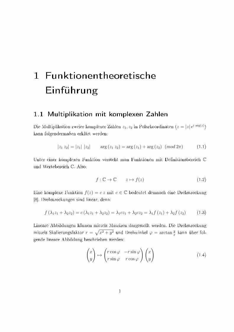
gende lineare Abbildung beschrieben werden:(x

y

)7→

(r cosϕ −r sinϕ

r sinϕ r cosϕ

)(x

y

)(1.4)

1

Di�erenzierbarkeit Konforme Abbildungen

Eine komplexe Zahl kann man also auch als Matrix au�assen.

c = a+ ib =̂

(a −bb a

)(1.5)

1.2 Di�erenzierbarkeit

Die Ableitung einer Funktion f(z) kann wie im Reellen mit Hilfe einer Grenzwertbil-

dung gefunden werden. Die Funktion f(z) ist in einem beliebigen Punkt z0 komplex

di�erenzierbar, wenn der Grenzwert

limz→z0

f(z)− f(z0)

z − z0= f ′(z0) (1.6)

existiert.

Wenn man den Isomorphismus zwischen R2 und C ausnützt, kann man die Funkti-

on f(z) = f(x+ iy) auch als Summe reller Funktionen

~f(x, y) =

(u(x, y)

v(x, y)

)=

(Re f(x+ iy)

Im f(x+ iy)

)(1.7)

darstellen, sodass f(x+ iy) = u(x, y) + i v(x, y).

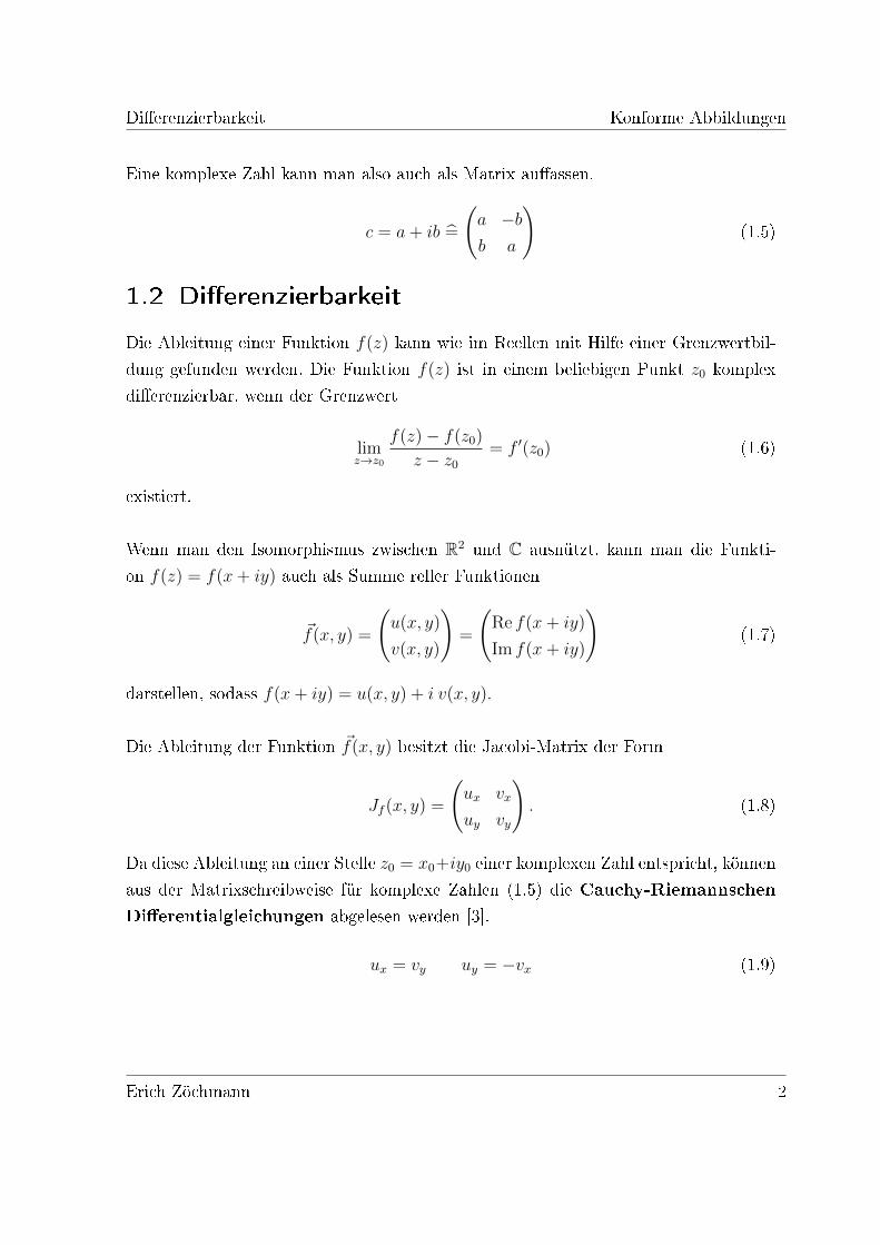
Die Ableitung der Funktion ~f(x, y) besitzt die Jacobi-Matrix der Form

Jf (x, y) =

(ux vx

uy vy

). (1.8)

Da diese Ableitung an einer Stelle z0 = x0+iy0 einer komplexen Zahl entspricht, können

aus der Matrixschreibweise für komplexe Zahlen (1.5) die Cauchy-Riemannschen

Di�erentialgleichungen abgelesen werden [3].

ux = vy uy = −vx (1.9)

Erich Zöchmann 2

Komplexes Potential Konforme Abbildungen

Ist Kε(z0) eine Kreisscheibe mit Mittelpunkt z0 und Radius ε > 0 und ist f(z), z ∈Kε(z0) komplex di�erenzierbar, so ist f holomorph.

Mit Hilfe des mehrdimensionalen Mittelwertsatzes und den Cauchy-Riemannschen Dif-

ferentialgleichungen lässt sich zeigen, dass man die komplexe Ableitung auch folgen-

dermaÿen de�nieren kann [6]:

f ′(z) = ux + i vx = vy − i uy (1.10)

Durch nochmaliges Anwenden der Cauchy-Riemannschen Di�erentialgleichungen kann

man die Ableitung rein über Real- oder Imaginärteile de�nieren [3].

f ′(z) = ux − i uy = vy + i vx (1.11)

1.3 Komplexes Potential

Für ein ebenes Vektorfeld

~F (x, y) =

(P (x, y)

Q(x, y)

)∼= P (x, y) + i Q(x, y) = F (x+ iy) (1.12)

ist die Funktion

ϕ : gradϕ = ~F (x, y) (1.13)

eine (reelle) Potentialfunktion. Für ein Vektorfeld mit Potentialfunktion müssen die

Integrabilitätsbedingungen gelten [6].

∂P (x, y)

∂y=∂Q(x, y)

∂y(1.14)

Dies ist gleichbedeutend mit rot ~F = ~0. Wenn eine Funktion ψ derart gefunden werden

kann, dass

f(z) = f(x+ iy) = ϕ(x, y) + iψ(x, y) (1.15)

Erich Zöchmann 3

Gebietstreue holomorpher Funktionen Konforme Abbildungen

holomorph ist, so kann f(z) als komplexes Potential gedeutet werden. Die Funktion

ψ(x, y) wird als konjugiert harmonische Funktion bezeichnet und ist bis auf eine addi-

tive Konstante eindeutig bestimmt. Das Vektorfeld ~F (x, y) kann aus der Gleichung

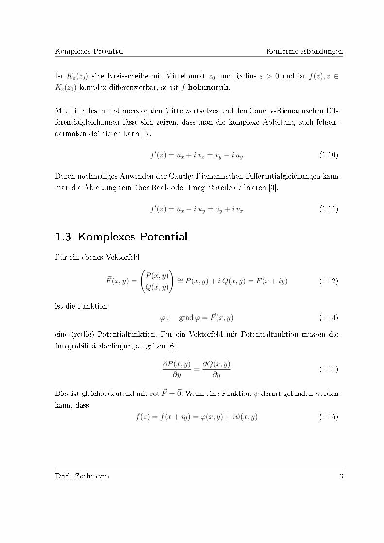
~F (x, y) = gradϕ(x, y) =

(ϕx

ϕy

)∼= ϕx + i ϕy = f(z)′ (1.16)

gewonnen werden. Die Niveaulinien ϕ(x, y) = c1 und ψ(x, y) = c2 schneiden einander

im rechten Winkel [8], da

〈gradϕ, gradψ〉 = 〈

(ϕx

ϕy

),

(ψx

ψy

)〉 = ϕx ψx + ϕy ψy = ϕx ψx + (−ψx) ϕx = 0 (1.17)

Dadurch lassen sich diese Niveaulinien physikalisch interpretieren. Die Niveaulinie

ϕ(x, y) = c1 entspricht einer Äquipotential�äche; ψ(x, y) = c2 einer Flusslinie.

1.4 Gebietstreue holomorpher Funktionen

Unter einem Gebiet G versteht man eine Teilmenge der komplexen Zahlenebene G ⊆ C,für die gilt [6]:

• G ist o�en.

• G ist zusammenhängend

• G 6= {}

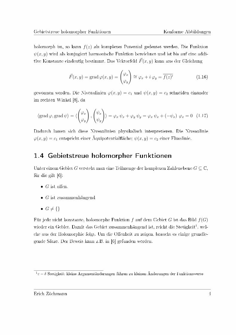
Für jede nicht konstante, holomorphe Funktion f auf dem Gebiet G ist das Bild f(G)

wieder ein Gebiet. Damit das Gebiet zusammenhängend ist, reicht die Stetigkeit1, wel-

che aus der Holomorphie folgt. Um die O�enheit zu zeigen, braucht es einige grundle-

gende Sätze. Der Beweis kann z.B. in [6] gefunden werden.

1ε− δ Stetigkeit: kleine Argumentänderungen führen zu kleinen Änderungen der Funktionswerte

Erich Zöchmann 4

Winkeltreue holomorpher Funtkionen Konforme Abbildungen

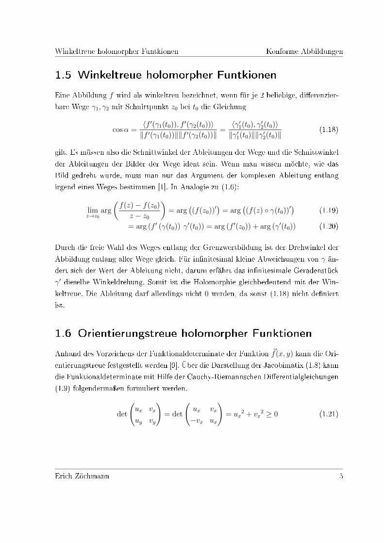
1.5 Winkeltreue holomorpher Funtkionen

Eine Abbildung f wird als winkeltreu bezeichnet, wenn für je 2 beliebige, di�erenzier-

bare Wege γ1, γ2 mit Schnittpunkt z0 bei t0 die Gleichung

cosα =〈f ′(γ1(t0)), f ′(γ2(t0))〉‖f ′(γ1(t0))‖‖f ′(γ2(t0))‖

=〈γ′1(t0), γ′2(t0)〉‖γ′1(t0)‖‖γ′2(t0)‖

(1.18)

gilt. Es müssen also die Schnittwinkel der Ableitungen der Wege und die Schnittwinkel

der Ableitungen der Bilder der Wege ident sein. Wenn man wissen möchte, wie das

Bild gedreht wurde, muss man nur das Argument der komplexen Ableitung entlang

irgend eines Weges bestimmen [1]. In Analogie zu (1.6):

limz→z0

arg

(f(z)− f(z0)

z − z0

)= arg

((f(z0))

′) = arg((f(z) ◦ γ(t0))

′) (1.19)

= arg (f ′ (γ(t0)) γ′(t0)) = arg (f ′(z0)) + arg (γ′(t0)) (1.20)

Durch die freie Wahl des Weges entlang der Grenzwertbildung ist der Drehwinkel der

Abbildung entlang aller Wege gleich. Für in�nitesimal kleine Abweichungen von γ än-

dert sich der Wert der Ableitung nicht, darum erfährt das in�nitesimale Geradenstück

γ′ dieselbe Winkeldrehung. Somit ist die Holomorphie gleichbedeutend mit der Win-

keltreue. Die Ableitung darf allerdings nicht 0 werden, da sonst (1.18) nicht de�niert

ist.

1.6 Orientierungstreue holomorpher Funktionen

Anhand des Vorzeichens der Funktionaldeterminate der Funktion ~f(x, y) kann die Ori-

entierungstreue festgestellt werden [9]. Über die Darstellung der Jacobimatix (1.8) kann

die Funktionaldeterminate mit Hilfe der Cauchy-Riemannschen Di�erentialgleichungen

(1.9) folgendermaÿen formuliert werden.

det

(ux vx

uy vy

)= det

(ux vx

−vx ux

)= ux

2 + vx2 ≥ 0 (1.21)

Erich Zöchmann 5

Orientierungstreue holomorpher Funktionen Konforme Abbildungen

Abbildung 1.1: Winkeltreue einer holomorphen Abbildung

Wobei die Funktionaldeterminate nur bei Nullstellen der Ableitung 0 werden kann.

Gra�k 1.1 zeigt neben der Winkeltreue auch die Orientierungstreue einer holomorphen

Abbildung.

Erich Zöchmann 6

2 Eigenschaften konformer

Abbildungen

2.1 Konformität

Eine Abbildung f(z) wird als konform auf dem Gebiet G bezeichnet, wenn ihre kom-

plexe Ableitung auf diesem Gebiet nirgends 0 ist, also:

f : G ⊆ C→ C f ′(z) 6= 0 ∀z ∈ G (2.1)

Durch diese Bedingung ist die Abbildung f(z) winkel- , gebiets- und orientierungstreu

(Kap. 1.5, Kap. 1.4 und Kap. 1.6). Um sich die Wirkung einer konformen Abildung zu

veranschaulichen, kann man von (1.6) ausgehen und die lineare Approximation um z0

betrachten [11].

f(z) ≈ f(z0) + f ′(z0) (z − z0) = f ′(z0)︸ ︷︷ ︸a

z+ f(z0)− f ′(z0) z0︸ ︷︷ ︸b

= a z+ b, a, b ∈ C (2.2)

Der Faktor a entspricht einer Drehstreckung und die Konstante b einer Translation.

2.2 Biholomorphe Funktionen

Eine biholomorphe Funktion ist eine bijektive holomorphe Funktion mit einer holomor-

phen Umkehrfunktion. Alle injektiven konformen Abbildungen sind auch biholomorph.

Durch die Gebietstreue ist die Surjektivität sichergestellt. Für die Ableitung der Um-

kehrfunktion gilt:

(f−1)′(w) =1

f ′(f−1(w))∀w ∈ f(G) (2.3)

7

Überlagerungs- und Verp�anzungsprinzip Konforme Abbildungen

Da die Ableitung der Funktion f(z) die Bedingung (2.1) erfüllt, ist auch die Umkehr-

funktion holomorph.

2.3 Überlagerungs- und Verp�anzungsprinzip

Das komplexe Potential hat dank der Ableitungsregeln zwei interessante Eigenschaften.

Durch die Linearität der Ableitung folgt die Überlagerungs- bzw Superpostionseigen-

schaft. Das Problem kann also in leichtere Teilprobleme überführt werden. Durch die

Kettenregel können schwierige in leichtere (bereits bekannte) Geometrien verp�anzt

werden. Für komplexe Potentiale f1, f2 in G gilt also [7]:

a, b ∈ C a f1 + b f2, ist komplexes Potential in G (2.4)

Weiters für ein komplexes Potential f im verp�anzten Gebiet A:

h : G→ A, h biholomorph, f ◦ h = f (h(z)) ist komplexes Potential in G (2.5)

Vorallem durch das Verp�anzungsprinzip entsteht die Motivation, sich seine Problem-

stellung mittels konformer Abbildungen zu vereinfachen.

2.4 Komposition konformer Abbildungen

Durch Komposition konformer Abbildungen können aufwendigere zusammengesetzt

werden. Für die konformen Abbildungen f1 und f2 kann mittels der Kettenregel die

Konformität der Komposition gezeigt werden.

f ′(z0) = (f1 ◦ f2)′ (z0) = (f1 (f2 (z0)))′ = f ′1 (f2(z0)) f

′2 (z0) (2.6)

Wenn f ′2 für alle z0 ∈ G und f ′1 für alle f2(z0) nirgendwo 0 werden, ist das Produkt

nullstellenfrei und die Komposition somit konform.

Erich Zöchmann 8

Riemannscher Abbbildungssatz Konforme Abbildungen

2.5 Riemannscher Abbbildungssatz

Zwei Gebiete werden als biholomorph äquivalent (bzw. konform äquivalent) bezeich-

net, wenn es zwischen ihnen eine biholomorphe Abbildung gibt [5]. Der Riemannsche

Abbildung 2.1: Darstellung Riemannscher Abbildungssatz

Abbildungssatz besagt, dass jedes einfach zusammenhängende Gebiet G 6= C biholo-

morph äquivalent zur o�enen Einheitskreisscheibe (|z| < 1) ist. Ein Gebiet heiÿt einfach

zusammenhängend, wenn sich jeder geschlossene Weg stetig auf einen Punkt zusam-

menziehen lässt [12]. In einfachen Worten - das Gebiet darf keine Löcher aufweisen.

Der Beweis des Riemanschen Abbildungssatzes ist hochgradig nicht-trivial! Dieser Satz

zeigt, dass eine konforme Abbildung zwischen zwei Gebieten existiert, weil jedes Gebiet

biholomorph auf die Einheitskreisscheibe D abgebildet werden kann. Eine Abbildung

f von A nach B lässt sich dann folgendermaÿen de�nieren:

g : A→ D h : B → D (2.7)

f : A→ B f = h−1 ◦ g (2.8)

Erich Zöchmann 9

3 Schwarz Christo�el

Transformation

Wenn man sein Problem mittels konformer Abbildungen lösen möchte, muss man in

Tabellen nach der geeigneten Transformation suchen, oder man �ndet durch geschicktes

Probieren die passende. Ganz anders verhält es sich, wenn das Problemgebiet durch

ein Polygon berandet ist. Die Schwarz Christo�el Formel liefert eine Rechenvorschrift,

mittels der die Transformation auf die komplexe Halbebene (Im z ≥ 0) - bis auf die

Auswertung eines Integrals - leicht gefunden werden kann.

3.1 Idee der Herleitung

Betrachtet man die Funktion f(z) mit der Ableitung,

f ′(z) = (z − x0)a, |a| < 1 (3.1)

so ist das Argument der Ableitung für rein reelle z (Im z ≡ 0)

arg f ′(z) = a arg (z − x0) =

0, wenn z ≥ x0

aπ, wenn z < x0.(3.2)

Das Argument kann so berechnet werden, da:

arg ((z − x0)a) = arg((|z − x0| ei arg(z−x0)

)a)= (3.3)

arg(|z − x0|a ei a arg(z−x0)

)= a arg(z − x0) (3.4)

Durch weitere Multiplikationen mit Termen der Art (3.1) können weitere Ecken erzeugt

10

Schwarz Christo�el Formel Konforme Abbildungen

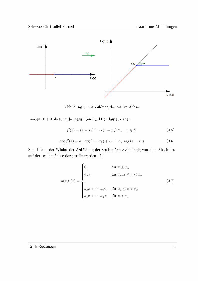
Abbildung 3.1: Abbildung der reellen Achse

werden. Die Ableitung der gesuchten Funktion lautet daher:

f ′(z) = (z − x0)a1 · · · (z − xn)an , n ∈ N (3.5)

arg f ′(z) = a1 arg (z − x0) + · · ·+ an arg (z − xn) (3.6)

Somit kann der Winkel der Abbildung der reellen Achse abhängig von dem Abschnitt

auf der reellen Achse dargestellt werden. [1]

arg f ′(z) =

0, für z ≥ xn

anπ, für xn−1 ≤ z < xn...

a2π + · · · anπ, für x1 ≤ z < x2

a1π + · · · anπ, für z < x1

(3.7)

Erich Zöchmann 11

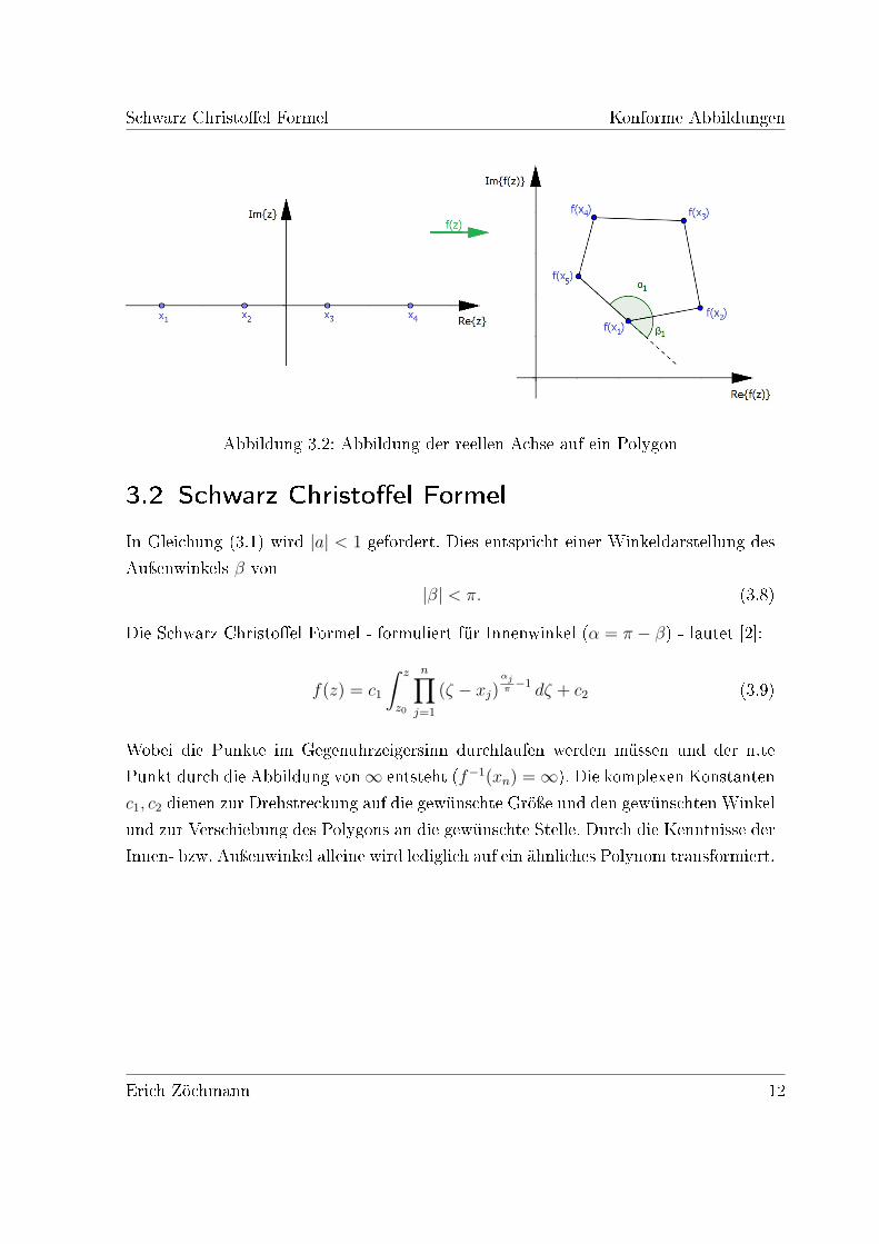
Schwarz Christo�el Formel Konforme Abbildungen

Abbildung 3.2: Abbildung der reellen Achse auf ein Polygon

3.2 Schwarz Christo�el Formel

In Gleichung (3.1) wird |a| < 1 gefordert. Dies entspricht einer Winkeldarstellung des

Auÿenwinkels β von

|β| < π. (3.8)

Die Schwarz Christo�el Formel - formuliert für Innenwinkel (α = π − β) - lautet [2]:

f(z) = c1

∫ z

z0

n∏j=1

(ζ − xj)αjπ−1 dζ + c2 (3.9)

Wobei die Punkte im Gegenuhrzeigersinn durchlaufen werden müssen und der n.te

Punkt durch die Abbildung von∞ entsteht (f−1(xn) =∞). Die komplexen Konstanten

c1, c2 dienen zur Drehstreckung auf die gewünschte Gröÿe und den gewünschten Winkel

und zur Verschiebung des Polygons an die gewünschte Stelle. Durch die Kenntnisse der

Innen- bzw. Auÿenwinkel alleine wird lediglich auf ein ähnliches Polynom transformiert.

Erich Zöchmann 12

4 Beispiele anhand

elektromagnetischer Felder

4.1 Laplacegleichung

Real- und Imaginärteil holomorpher Funktionen erfüllen die Laplacegleichung. Für die

Funktion f(x+ i y) = u(x, y) + i v(x, y) gilt durch (1.9) und dem Satz von Schwarz [6]:

∆u = (ux)x + (uy)y = (vy)x + (−vx)y = 0 (4.1)

∆v = (vx)x + (vy)y = (−uy)x + (ux)y = 0 (4.2)

Wenn der Laplaceoperator auf f angewandt wird, ergibt sich wegen der Linearität des

Laplaceoperators:

∆f(x+ i y) = ∆u(x, y) + i∆v(x, y) = 0 + i 0 (4.3)

Jede holomorphe Funktion erfüllt somit die Laplacegleichung

∆f(z) = 0 (4.4)

Als holomorphe Funktion bietet sich das komplexe Potential (Kap. 1.3) an.

4.2 Elektrostatik

In der Elektrostatik müssen die Gleichungen

rot ~E = ~0 div ~D = 0 (4.5)

13

Elektrostatik Konforme Abbildungen

gelten, damit man die Laplacegleichung

0 = div ~D = div ε ~E = −ε div gradϕ = −ε∆ϕ (4.6)

formulieren kann ( ~D = ε ~E, ~E = − gradϕ). Durch diese Einschränkung dürfen sich

in dem zu lösenden Gebiet nirgends Ladungen be�nden, da sonst die Laplacegleichung

durch die Poissongleichung zu ersetzen wäre. (div ~D = ρ)

∆ϕ = −ρε

(4.7)

4.2.1 Zylinderkondensator

Anhand eines illustrativen Beispiels wird die Vorteilhaftigkeit von konformen Abbil-

dungen gezeigt. Die Kapazität eines Zylinderkondensators kann auch auf herkömmli-

che Weise - dank der Symmetrie - über das elektrische Feld einer Punktladung und

mittels Integration gewonnen werden. Das hier gezeigte Verfahren kann allerdings auch

auf beliebige Geometrie angewendet werden, sofern eine konforme Abbildung gefun-

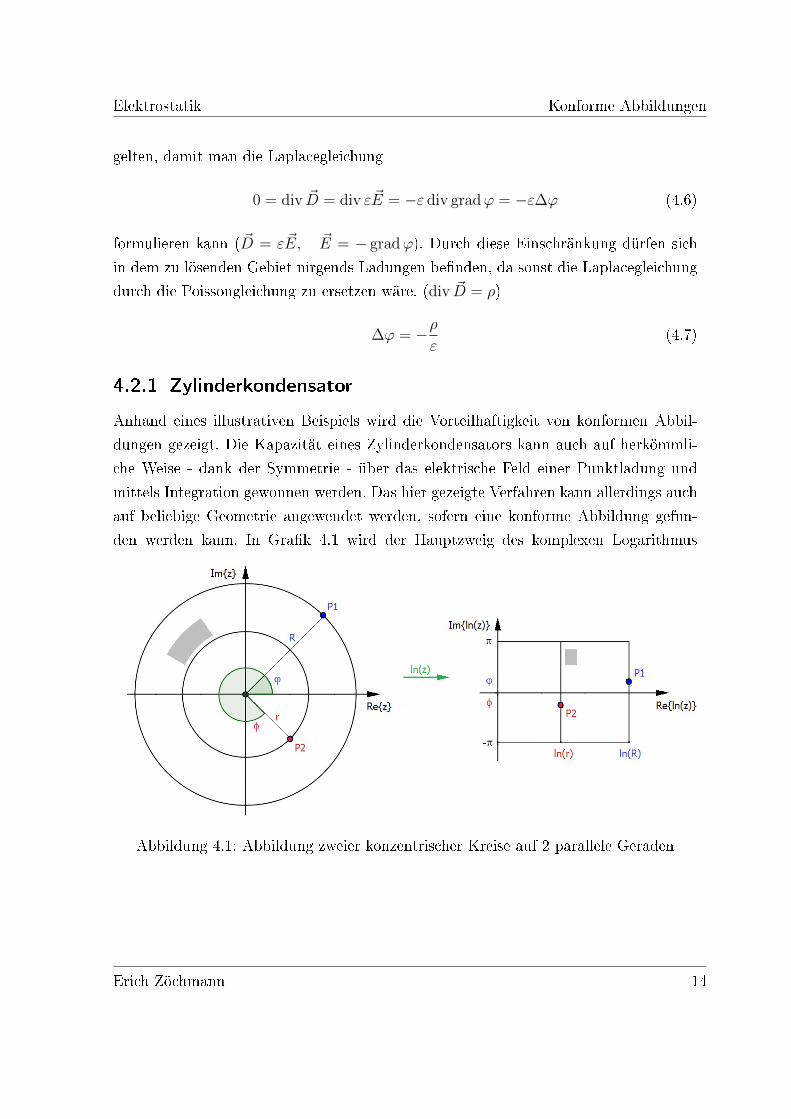
den werden kann. In Gra�k 4.1 wird der Hauptzweig des komplexen Logarithmus

Abbildung 4.1: Abbildung zweier konzentrischer Kreise auf 2 parallele Geraden

Erich Zöchmann 14

Elektrostatik Konforme Abbildungen

(π < Im ln(z) < π) benutzt. Dieser lässt sich wie folgt berechnen:

ln(z) = ln(|z| ei arg(z)

)= ln(|z|) + i arg(z) (4.8)

Die Koordinaten des Urbildes aus den Bildkoordinaten (u = Re ln(z), v = Im ln(z))

berechnen sich folgendermaÿen:

x+ i y = eu+i v = eu ei v = eu (cos v + i sin v) (4.9)

Mittels Gleichung (4.9) erhält man die Gleichung des konzentrischen Kreises.

x2 + y2 = (eu cos v)2 + (eu sin v)2 = e2u(cos2 v + sin2 v

)= e2u (4.10)

Damit lassen sich die Koordinaten der Realteile der parallelen Geradenstücke leicht

berechnen. Über die bekannte Formel für den Plattenkondensator und der Länge l der

Anordung berechnet sich die Kapazität zu:

C =ε A

d=

ε 2π l

lnR− ln r=

2π ε l

ln Rr

(4.11)

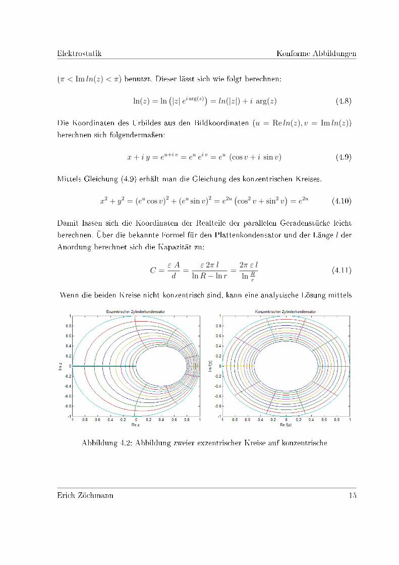
Wenn die beiden Kreise nicht konzentrisch sind, kann eine analytische Lösung mittels

Abbildung 4.2: Abbildung zweier exzentrischer Kreise auf konzentrische

Erich Zöchmann 15

Magnetostatik Konforme Abbildungen

Integration des elektrischen Feldes einer Punktladung nicht mehr gewonnen werden1.

Da die Komposition von konformen Abbildung wieder konform ist (siehe Kap. 2.4),

kann mit Hilfe einer weiteren konformen Abbildung die Exzentrizität aufgehoben wer-

den. Die Gra�k 4.2 zeigt die Äquipotential�ächen und die Flusslinien der Abbildung

f(z) = z−z0z0z−1 , z0 = 1

2[3].

4.3 Magnetostatik

Für die Magnetostatik gibt es ähnliche Einschränkungen an die Maxwell Gleichungen

wie in der Elektrostatik.

rot ~H = ~0 div ~B = 0 (4.12)

0 = div ~B = div µ ~H = −µ div gradϕm = −µ∆ϕm (4.13)

( ~B = µ ~H, ~H = − gradϕm) Hier muss die Rotation von ~H verschwinden, wodurch

nur stromfreie Gebiete gelöst werden können. Wenn man den Strom berücksichtigen

möchte, kann man kein skalares Potential ϕm mehr angeben; die Lösung kann mittels

der vorgestellten Methode nicht gefunden werden. 2

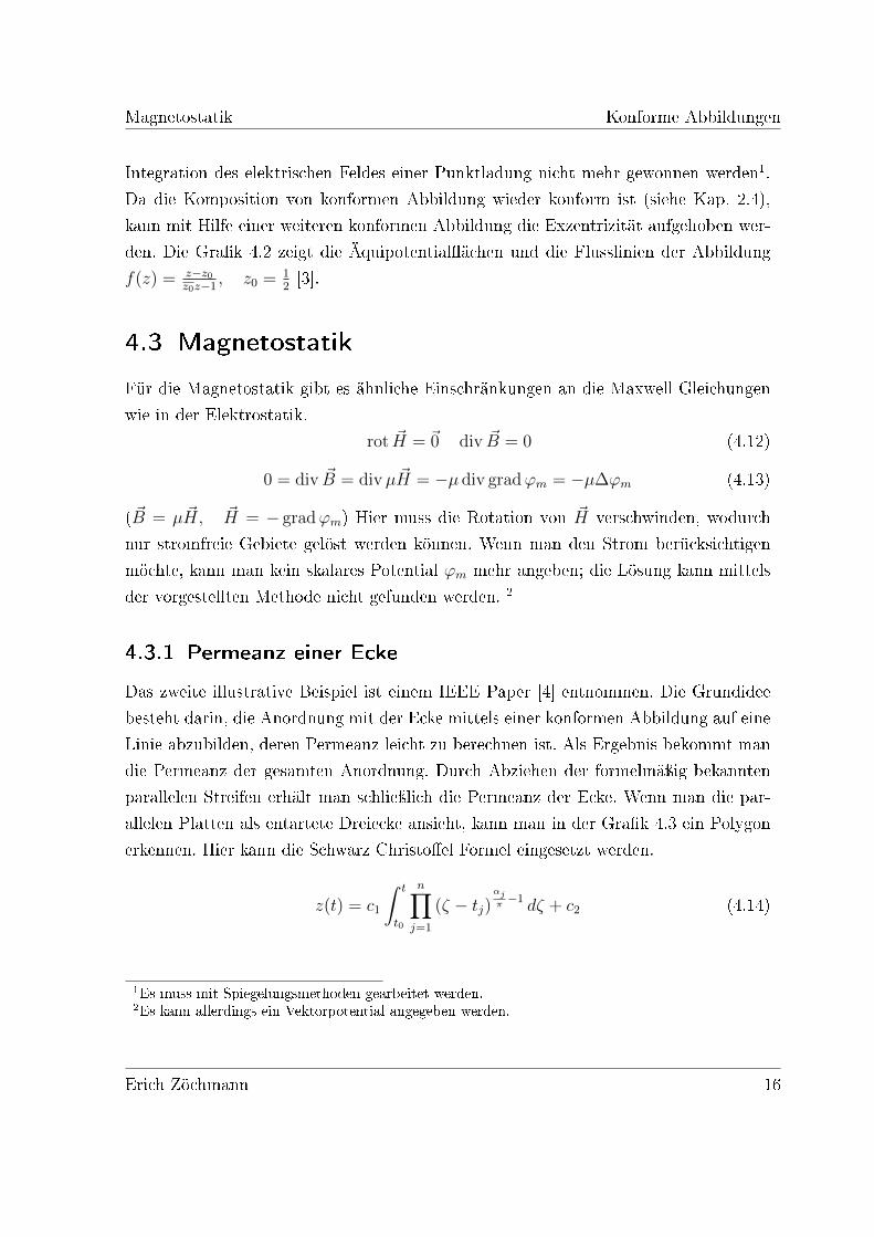
4.3.1 Permeanz einer Ecke

Das zweite illustrative Beispiel ist einem IEEE Paper [4] entnommen. Die Grundidee

besteht darin, die Anordnung mit der Ecke mittels einer konformen Abbildung auf eine

Linie abzubilden, deren Permeanz leicht zu berechnen ist. Als Ergebnis bekommt man

die Permeanz der gesamten Anordnung. Durch Abziehen der formelmäÿig bekannten

parallelen Streifen erhält man schlieÿlich die Permeanz der Ecke. Wenn man die par-

allelen Platten als entartete Dreiecke ansieht, kann man in der Gra�k 4.3 ein Polygon

erkennen. Hier kann die Schwarz Christo�el Formel eingesetzt werden.

z(t) = c1

∫ t

t0

n∏j=1

(ζ − tj)αjπ−1 dζ + c2 (4.14)

1Es muss mit Spiegelungsmethoden gearbeitet werden.2Es kann allerdings ein Vektorpotential angegeben werden.

Erich Zöchmann 16

Magnetostatik Konforme Abbildungen

Abbildung 4.3: Schwarz Christo�el Abbildung einer Ecke

z(t) = c1

∫ t

t0

(ζ − δ2

) π2π−1

(ζ + 1)3π2π−1 (ζ − 0)0−1 dζ + c2 (4.15)

= c1

∫ t

t0

√ζ + 1√ζ − δ2 ζ

dζ + c2 (4.16)

Durch Abbildung von ∞ entsteht Punkt 4. Im IEEE Paper [4] wird

z(t) =2δ

π

[1

δarctan

(uδ

)+ artanh(u)

], u =

√t− δ2t+ 1

(4.17)

als Transformation angegeben. Um zu zeigen, dass diese Abbildung mit (4.15) überein-

stimmt, wird (4.17) di�erenziert. Durch mehrmaliges Anwenden der Kettenregel und

Umstellen der Terme erhält man:

z′(t) =2

π

[arctan

(ud

)]′+

2δ

π[artanh(u)]′ (4.18)

=δ

π

1

t(t+ 1)u+δ

π

1

(t+ 1)u=δ

π

1

(t+ 1)u

(1

t+ 1

)(4.19)

=δ

π

1

(t+ 1)u

(1 + t

t

)=δ

π

1

u t=δ

π

√t+ 1√t− δ2 t

(4.20)

Erich Zöchmann 17

Magnetostatik Konforme Abbildungen

Wenn man c1 mit δπindenti�ziert und c2 mit 0, erhält man den Integranden von (4.15).

In der t-Ebene kann das Potential durch einen Ansatz der Form

f(t) = c1 ln(t) + c2 (4.21)

formuliert werden [10]. Durch die Randbedingungen bei arg(t) = π, Im f(t) = U0 und

arg(t) = 0, Im f(t) = 0 kann die Lösung des Potentials gefunden werden.

f(t) =U0

πln(t) =

U0

π(ln |x+ i y|+ i arg(x+ i y)) (4.22)

=U0

π

ln(√

x2 + y2)

︸ ︷︷ ︸u(x,y)

+i arctan(yx

)︸ ︷︷ ︸

v(x,y)

(4.23)

Abhängig vom Quadranten muss beim arctan noch π addiert werden. Dieses Potential

erfüllt die Cauchy-Riemannschen Di�erentialgleichungen, da

ux =1√

x2 + y22x

2√x2 + y2

=x

x2 + y2(4.24)

uy =1√

x2 + y22y

2√x2 + y2

=y

x2 + y2(4.25)

vx =1

1 +(yx

)2 y

−x2=

−yx2 + y2

(4.26)

vy =1

1 +(yx

)2 1

x=

x

x2 + y2. (4.27)

Das gefundene Potential ist somit holomorph und erfüllt dadurch die Kriterien eines

komplexen Potentials. Aus rot ~B = ~0 folgt die Existenz eines Skalarpotentials ϕm ( ~B =

−µ gradϕm) und aus div ~B = 0 die Existenz eines Vektorpotentials A ( ~B = rot ~A),

welches durch das ebene Problem z gerichtet ist( ~A = Az ~ez). Die magnetische Fluÿdichte

lässt sich somit über

~B =

(∂Az∂y

−∂Az∂x

)=

(−µ ∂ϕm

∂x

−µ ∂ϕm∂y

)(4.28)

Erich Zöchmann 18

Magnetostatik Konforme Abbildungen

ausdrücken. Damit die Cauchy-Riemannschen Di�erentialgleichungen erfüllt sind, muss

das komplexe Potential eine der folgenden Formen aufweisen:

f(z) = µ ϕm − i Az (4.29)

f(z) = −µ ϕm + i Az (4.30)

f(z) = Az + i µ ϕm (4.31)

f(z) = −Az − i µ ϕm (4.32)

Die Autoren von [4] haben sich für die Variante (4.31) entschieden. Die magnetische

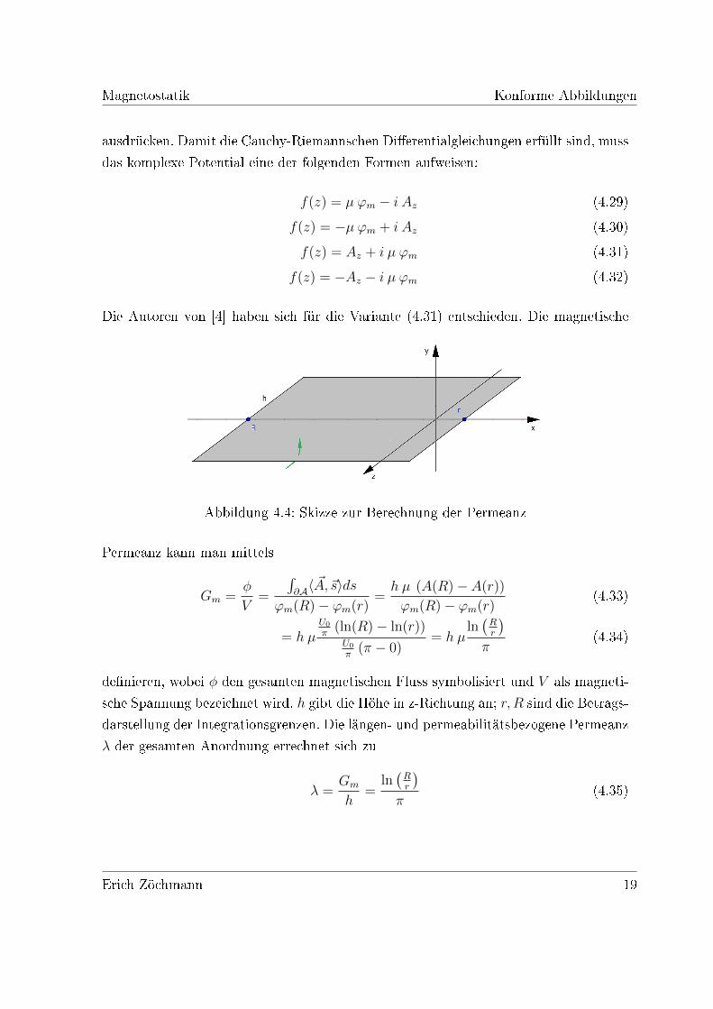
Abbildung 4.4: Skizze zur Berechnung der Permeanz

Permeanz kann man mittels

Gm =φ

V=

∫∂A〈 ~A,~s〉ds

ϕm(R)− ϕm(r)=h µ (A(R)− A(r))

ϕm(R)− ϕm(r)(4.33)

= h µU0

π(ln(R)− ln(r))U0

π(π − 0)

= h µln(Rr

)π

(4.34)

de�nieren, wobei φ den gesamten magnetischen Fluss symbolisiert und V als magneti-

sche Spannung bezeichnet wird. h gibt die Höhe in z-Richtung an; r, R sind die Betrags-

darstellung der Integrationsgrenzen. Die längen- und permeabilitätsbezogene Permeanz

λ der gesamten Anordnung errechnet sich zu

λ =Gm

h=

ln(Rr

)π

(4.35)

Erich Zöchmann 19

Magnetostatik Konforme Abbildungen

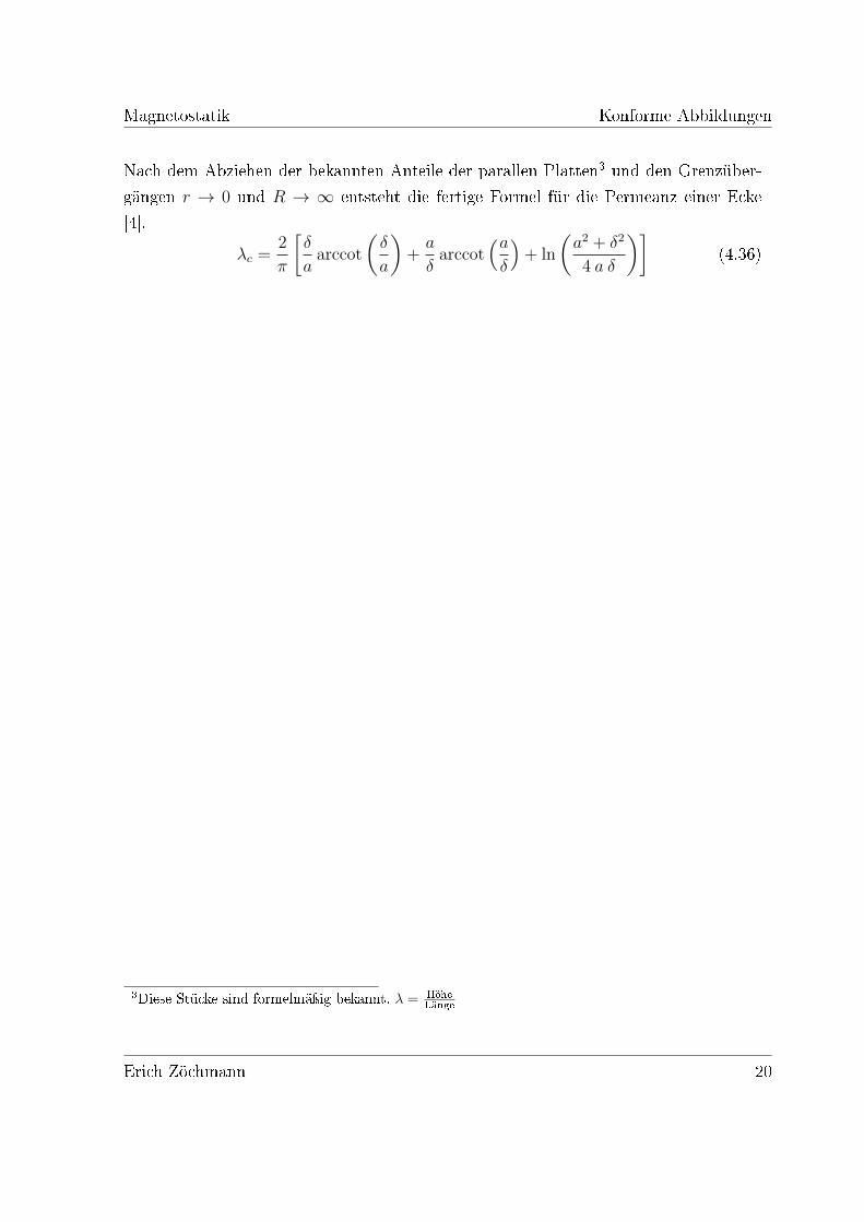
Nach dem Abziehen der bekannten Anteile der parallen Platten3 und den Grenzüber-

gängen r → 0 und R → ∞ entsteht die fertige Formel für die Permeanz einer Ecke

[4].

λc =2

π

[δ

aarccot

(δ

a

)+a

δarccot

(aδ

)+ ln

(a2 + δ2

4 a δ

)](4.36)

3Diese Stücke sind formelmäÿig bekannt. λ = HöheLänge

Erich Zöchmann 20

Abbildungsverzeichnis

1.1 Winkeltreue einer holomorphen Abbildung . . . . . . . . . . . . . . . . 6

2.1 Darstellung Riemannscher Abbildungssatz . . . . . . . . . . . . . . . . 9

3.1 Abbildung der reellen Achse . . . . . . . . . . . . . . . . . . . . . . . . 11

3.2 Abbildung der reellen Achse auf ein Polygon . . . . . . . . . . . . . . . 12

4.1 Abbildung zweier konzentrischer Kreise auf 2 parallele Geraden . . . . 14

4.2 Abbildung zweier exzentrischer Kreise auf konzentrische . . . . . . . . . 15

4.3 Schwarz Christo�el Abbildung einer Ecke . . . . . . . . . . . . . . . . . 17

4.4 Skizze zur Berechnung der Permeanz . . . . . . . . . . . . . . . . . . . 19

A

Literaturverzeichnis

[1] William Chen. Introduction to Complex Analysis. Sydney, 1996.

[2] George F. Carrier et. al., editor. functions of a complex variable. mcgraw-hill

book, inc., New York, 1 edition, 1966.

[3] Tilo Arens et. al., editor. Mathematik. Spektrum Akademischer Verlag, Heidelberg,

1 edition, 2008.

[4] G.A. Cividjian et.al. Some Formulas for Two-Dimensional Permeances. IEEE

Transactions on Magnetics, 36:3754�3758, 2000.

[5] Dirk Ferus. Komplexe Analysis. TU Berlin, 2010.

[6] Stefan Krause and Andreas Körner. Komplexe Analysis. TU Wien, 2010.

[7] Kurt Meyberg and Peter Vachenauer, editors. Höhere Mathematik 2. Springer,

Berlin Heidelberg New York, 4 edition, 2001.

[8] Jerrold E. Marsden and Michael J. Ho�man, editors. BASIC COMPLEX ANA-

LYSIS. W.H. Freeman and Company, New York, 2 edition, 1987.

[9] Peter Szmolyan. Mathematik 2 für ET. TU Wien, 2010.

[10] Josef Timmerberg. Einsatz von FemLab in der Elektrotechnikausbildung. COM-

SOL Multiphysics Conference, 2005.

[11] Hans Walser. Konforme Abbildungen. ETH Zürich, 2002.

[12] Wikipedia. Zusammenhängender Raum. http://de.wikipedia.org/wiki/

Zusammenhängender_Raum. letzer Abruf: 22. September 2011.

B

3754 IEEE TRANSACTIONS ON MAGNETICS, VOL. 36, NO. 5, SEPTEMBER 2000

Some Formulas for Two-Dimensional PermeancesG. A. Cividjian, A. G. Cividjian, and N. G. Silvis-Cividjian

Abstract—By using a conformal mapping, the variation of theelectric or magnetic field in gaps near a corner is studied, andsome formulas for two-dimensional (2-D) “corner” and “constric-tion” permeances are proposed. The formulas offer the possibilityof making more accurate analytical calculations of magnetic cir-cuits and to better evaluate magnetic forces acting in plunger mag-nets.

Index Terms—Actuator, conformal mapping, partial capacity,permeance, two-dimensional electric and magnetic field.

I. INTRODUCTION

OFTEN, the boundary of the region in which the electricor magnetic field has to be solved contains small gaps

in which the field is strongly nonuniform, increasing theo-retically to infinity near the corners. In these cases, the finiteelement method (FEM) requires too many nodes for accuratecomputation.

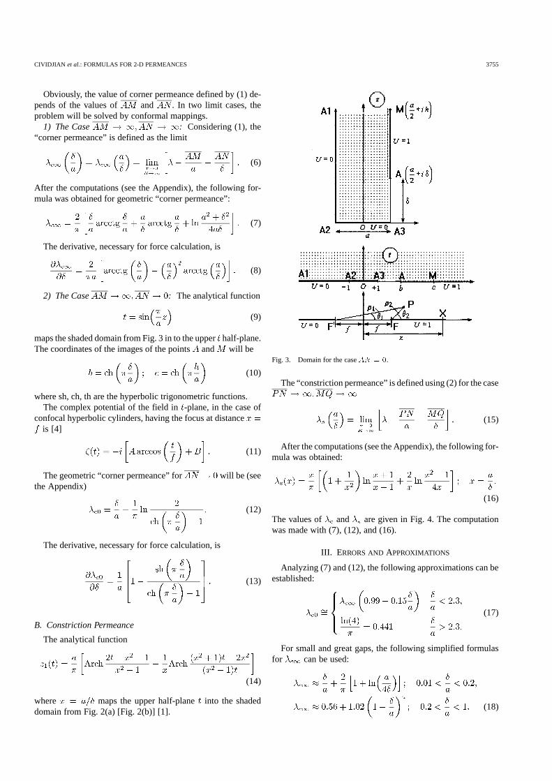
In this paper, two situations are studied: the “corner perme-ance” [Fig. 1(a)] and the “constriction permeance” [Fig. 2(a)].For the rest of the domain, where the field is more uniform, theFEM can be used. In order to break the field into flux paths,the border between the two regions must coincide with a fieldline.

Far enough from the edge, the field can be considered uniformand the field lines straightforward. In this condition, the two-dimensional (2-D) geometric permeance of the shaded part inFig. 1(a) can be presented as a sum of three terms

(1)

We will call “corner permeance” and will calculate it asa difference between the total permeance, determined usinga conformal mapping, and the first two terms of the aboveequation.

In the same way, the 2-D geometric permeance of the shadedpart in Fig. 2(a) can be written as a sum of the following threeterms:

(2)

where will be called “constriction permeance.”

Manuscript received December 6, 1999; revised April 28, 2000.The authors are with the University of Craiova, RO-1100 Craiova, Romania

(e-mail: gcividjian@elth.ucv.ro).Publisher Item Identifier S 0018-9464(00)08179-6.

Fig. 1. Domain of the map for “corner permeance.”

Fig. 2. Domain of the map for “constriction permeance.”

II. THE FIELD PROBLEM

A. Corner Permeance

For , the complex function

(3)

maps the shaded domain from Fig. 1(a) into upper half-plane[Fig. 1(b)] [1].

Considering the half-axes and in the -plane having,respectively, the potential and 0, the complex potential of thefield will be

(4)

where is the flux function and is the magnetic potential. Thetotal geometric permeance, between the area and thecorresponding area on [Fig. 1(a)], is given by the equation

(5)

0018–9464/00$10.00 © 2000 IEEE

CIVIDJIAN et al.: FORMULAS FOR 2-D PERMEANCES 3755

Obviously, the value of corner permeance defined by (1) de-pends of the values of and . In two limit cases, theproblem will be solved by conformal mappings.

1) The Case : Considering (1), the“corner permeance” is defined as the limit

(6)

After the computations (see the Appendix), the following for-mula was obtained for geometric “corner permeance”:

(7)

The derivative, necessary for force calculation, is

(8)

2) The Case : The analytical function

(9)

maps the shaded domain from Fig. 3 in to the upperhalf-plane.The coordinates of the images of the pointsand will be

(10)

where sh, ch, th are the hyperbolic trigonometric functions.The complex potential of the field in-plane, in the case of

confocal hyperbolic cylinders, having the focus at distanceis [4]

(11)

The geometric “corner permeance” for will be (seethe Appendix)

(12)

The derivative, necessary for force calculation, is

(13)

B. Constriction Permeance

The analytical function

(14)

where maps the upper half-planeinto the shadeddomain from Fig. 2(a) [Fig. 2(b)] [1].

Fig. 3. Domain for the caseAN = 0.

The “constriction permeance” is defined using (2) for the case

(15)

After the computations (see the Appendix), the following for-mula was obtained:

(16)

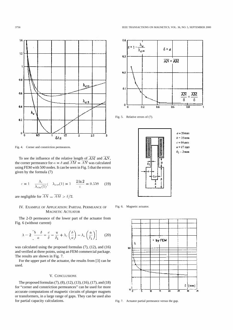
The values of and are given in Fig. 4. The computationwas made with (7), (12), and (16).

III. ERRORS ANDAPPROXIMATIONS

Analyzing (7) and (12), the following approximations can beestablished:

(17)

For small and great gaps, the following simplified formulasfor can be used:

(18)

3756 IEEE TRANSACTIONS ON MAGNETICS, VOL. 36, NO. 5, SEPTEMBER 2000

Fig. 4. Corner and constriction permeances.

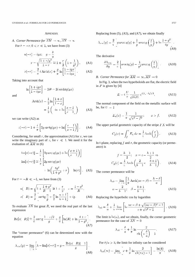
To see the influence of the relative length of and ,the corner permeance for and was calculatedusing FEM with 500 nodes. It can be seen in Fig. 5 that the errorsgiven by the formula (7)

(19)

are negligible for .

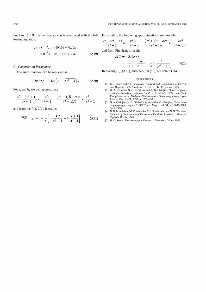
IV. EXAMPLE OF APPLICATION: PARTIAL PERMEANCE OF

MAGNETIC ACTUATOR

The 2-D permeance of the lower part of the actuator fromFig. 6 (without current)

(20)

was calculated using the proposed formulas (7), (12), and (16)and verified at three points, using an FEM commercial package.The results are shown in Fig. 7.

For the upper part of the actuator, the results from [3] can beused.

V. CONCLUSIONS

The proposed formulas (7), (8), (12), (13), (16), (17), and (18)for “corner and constriction permeances” can be used for moreaccurate computations of magnetic circuits of plunger magnetsor transformers, in a large range of gaps. They can be used alsofor partial capacity calculations.

Fig. 5. Relative errors of (7).

Fig. 6. Magnetic actuator.

Fig. 7. Actuator partial permeance versus the gap.

CIVIDJIAN et al.: FORMULAS FOR 2-D PERMEANCES 3757

APPENDIX

A. Corner Permeance for

For , we have from (3)

(A1)

(A2)

Taking into account that

and

(A3)

we can write (A2) as

(A4)

Considering, for small , the approximation (A1) for , we canwrite the imaginary part of , for . We need it for theevaluation of in (6)

(A5)

For , we have from (3)

(A6)

To evaluate for great , we need the real part of the lastexpression

(A7)

The “corner permeance” (6) can be determined now with theequation

(A8)

Replacing from (5), (A5), and (A7), we obtain finally

(A9)

The derivative

(A10)

B. Corner Permeance for

In Fig. 3, when the two hyperboloids are flat, the electric fieldin is given by [4]

(A11)

The normal component of the field on the metallic surface willbe, for

(A12)

The upper partial geometric capacity of the stripe will be

(A13)

In -plane, replacing and , the geometric capacity (or perme-ance) is

(A14)

The corner permeance will be

(A15)

Replacing the hyperbolic cos by logarithm

(A16)

The limit is , and we obtain, finally, the corner geometricpermeance for the case of

(A17)

For , the limit for infinity can be considered

(A18)

3758 IEEE TRANSACTIONS ON MAGNETICS, VOL. 36, NO. 5, SEPTEMBER 2000

For , this permeance can be evaluated with the fol-lowing equation:

(A19)

C. Constriction Permeance

The Arch function can be replaced as

(A20)

For great , we can approximate

and from the Fig. 2(a), it results

(A21)

For small , the following approximations are possible:

and from Fig. 2(a), it results

(A22)

Replacing (5), (A21), and (A22) in (15), we obtain (16).

REFERENCES

[1] K. J. Binns and P. J. Lawrenson,Analysis and Computation of Electricand Magnetic Field Problems. Oxford, U.K.: Pergamon, 1963.

[2] G. A. Cividjian, N. G. Cividjian, and A. G. Cividjian, “Power approxi-mation of boundary conditions,” inProc. NUMELEC 97 Seconde Conf.Européenne sur les Méthodes Numériques en Electromagnétisme, Lyon,France, Mar. 19–21, 1997, pp. 252–253.

[3] G. A. Cividjian, N. G. Silvis-Cividjian, and A. G. Cividjian, “Inductanceof plungertype magnet,”IEEE Trans. Magn., vol. 34, pp. 3685–3688,Sept. 1998.

[4] N. N. Miroliubov, M. V. Kostenko, M. L. Levinstein, and N. N. Tihodeev,Methods of Computation of Elctrostatic Fields(in Russian). Moscow:Vyshaia Shkola, 1963.

[5] H. C. Roters,Electromagnetic Devices. New York: Wiley, 1967.