Information in Intelligent Transportation Systems

Information in Intelligent

Transportation Systems

Vom Fachbereich Physik – Technologie der Universitat –Gesamthochschule-Duisburg zur Erlangung des akademischen Grades eines

Doktors der Naturwissenschaften genehmigte Inaugural-Dissertation

vorgelegt von

Joachim Wahle

aus Winterberg (Sauerland)

Referent: Prof. Dr. M. SchreckenbergKorreferent: Prof. Dr. D. E. WolfTag der mundlichen Prufung: 15.01.02

Contents

0.1 Introduction . . . . . . . . . . . . . . . . . . . . . . . . . . . . 10.2 Objectives of the Thesis . . . . . . . . . . . . . . . . . . . . . 20.3 Thesis Outline . . . . . . . . . . . . . . . . . . . . . . . . . . . 3

1 Intelligent Transportation System 51.1 Introduction . . . . . . . . . . . . . . . . . . . . . . . . . . . . 5

1.1.1 ITS Areas . . . . . . . . . . . . . . . . . . . . . . . . . 61.1.2 Detection Devices . . . . . . . . . . . . . . . . . . . . . 71.1.3 Technologies . . . . . . . . . . . . . . . . . . . . . . . . 81.1.4 Temporal Nature of Information . . . . . . . . . . . . . 81.1.5 Information in Traffic Systems . . . . . . . . . . . . . 9

1.2 Advanced Traffic Management Systems . . . . . . . . . . . . 101.3 Advanced Traveller Information Systems . . . . . . . . . . . . 11

1.3.1 Possible Influences on Travel Behaviour . . . . . . . . . 131.3.2 Potential Benefits . . . . . . . . . . . . . . . . . . . . . 141.3.3 Potential Drawbacks . . . . . . . . . . . . . . . . . . . 15

1.4 Discussion . . . . . . . . . . . . . . . . . . . . . . . . . . . . . 16

2 Agents in the Traffic Domain 172.1 Basic Concepts . . . . . . . . . . . . . . . . . . . . . . . . . . 17

2.1.1 What is an Agent? . . . . . . . . . . . . . . . . . . . . 182.1.2 Environment . . . . . . . . . . . . . . . . . . . . . . . 192.1.3 Types of Agents . . . . . . . . . . . . . . . . . . . . . 202.1.4 Multi-Agent Systems . . . . . . . . . . . . . . . . . . . 212.1.5 Cooperation and Coordination . . . . . . . . . . . . . 21

2.2 Applications . . . . . . . . . . . . . . . . . . . . . . . . . . . . 222.2.1 Scheduling Problems . . . . . . . . . . . . . . . . . . . 222.2.2 Urban Traffic Control . . . . . . . . . . . . . . . . . . . 242.2.3 Road Traffic Management . . . . . . . . . . . . . . . . 26

i

ii CONTENTS

2.3 Driver Models . . . . . . . . . . . . . . . . . . . . . . . . . . 272.3.1 Is a Road User an Agent? . . . . . . . . . . . . . . . . 282.3.2 Classical Traffic Flow Models . . . . . . . . . . . . . . 282.3.3 Requirements in Knowledge-Based Applications . . . . 322.3.4 Cognitive Driver Models . . . . . . . . . . . . . . . . . 33

2.4 Two-Layer Architecture . . . . . . . . . . . . . . . . . . . . . 352.4.1 Tactical Layer . . . . . . . . . . . . . . . . . . . . . . . 362.4.2 Strategic Layer . . . . . . . . . . . . . . . . . . . . . . 362.4.3 Case Study 1: Anticipatory Traffic Forecast . . . . . . 372.4.4 Case Study 2: Application to Crowd Motion . . . . . . 39

2.5 Discussion . . . . . . . . . . . . . . . . . . . . . . . . . . . . . 41

3 Pre-Trip Information 433.1 Coordination Games . . . . . . . . . . . . . . . . . . . . . . . 43

3.1.1 El Farol Bar Problem . . . . . . . . . . . . . . . . . . . 443.1.2 Minority Game . . . . . . . . . . . . . . . . . . . . . . 45

3.2 Commuter Scenario . . . . . . . . . . . . . . . . . . . . . . . 463.3 Personalities . . . . . . . . . . . . . . . . . . . . . . . . . . . 473.4 Results . . . . . . . . . . . . . . . . . . . . . . . . . . . . . . . 49

3.4.1 Homogeneous Societies . . . . . . . . . . . . . . . . . . 493.4.2 Heterogeneous Societies . . . . . . . . . . . . . . . . . 50

3.5 Hamming Distance . . . . . . . . . . . . . . . . . . . . . . . . 523.5.1 Hamming Distance of Personalities . . . . . . . . . . . 52

3.6 Real Data on Route Choice Behaviour . . . . . . . . . . . . . 543.6.1 Surveys . . . . . . . . . . . . . . . . . . . . . . . . . . 543.6.2 Route Choice Simulators . . . . . . . . . . . . . . . . . 553.6.3 Laboratory Experiments . . . . . . . . . . . . . . . . . 55

3.7 Conclusion . . . . . . . . . . . . . . . . . . . . . . . . . . . . . 57

4 En-Route Information 594.1 Two-Route Scenario . . . . . . . . . . . . . . . . . . . . . . . 59

4.1.1 Simulation Technique . . . . . . . . . . . . . . . . . . . 614.2 Floating-Car Data . . . . . . . . . . . . . . . . . . . . . . . . 64

4.2.1 Influence of the Length . . . . . . . . . . . . . . . . . . 664.2.2 Influence of the Injection Rate . . . . . . . . . . . . . . 674.2.3 Influence of the Floating Cars (FCs) . . . . . . . . . . 684.2.4 Influence of the Deceleration Probability . . . . . . . . 694.2.5 Influence of the Dynamic Drivers . . . . . . . . . . . . 71

CONTENTS iii

4.2.6 Influence of the Static Drivers . . . . . . . . . . . . . . 724.3 Different Criteria . . . . . . . . . . . . . . . . . . . . . . . . . 74

4.3.1 Gradient of Travel Time . . . . . . . . . . . . . . . . . 744.3.2 Global Density and Speed . . . . . . . . . . . . . . . . 764.3.3 Comparison . . . . . . . . . . . . . . . . . . . . . . . . 79

4.4 Summary . . . . . . . . . . . . . . . . . . . . . . . . . . . . . 79

5 ATIS 835.1 Principle of On-Line Simulations . . . . . . . . . . . . . . . . 835.2 Freeway Simulator . . . . . . . . . . . . . . . . . . . . . . . . 85

5.2.1 Agent-Based Model . . . . . . . . . . . . . . . . . . . . 855.2.2 Network Structure . . . . . . . . . . . . . . . . . . . . 875.2.3 Tuning Methods . . . . . . . . . . . . . . . . . . . . . 87

5.3 Results . . . . . . . . . . . . . . . . . . . . . . . . . . . . . . . 895.3.1 Application to North Rhine-Westphalia . . . . . . . . . 905.3.2 Simulation Speed . . . . . . . . . . . . . . . . . . . . . 915.3.3 Traffic Demand Data . . . . . . . . . . . . . . . . . . . 915.3.4 Consistency of the Results . . . . . . . . . . . . . . . . 915.3.5 Dynamic Route Guidance Systems (DRGS) . . . . . . 93

5.4 Traffic Forecast . . . . . . . . . . . . . . . . . . . . . . . . . . 935.4.1 Dynamic Traffic Forecast . . . . . . . . . . . . . . . . . 945.4.2 Historical Data in Urban Areas . . . . . . . . . . . . . 965.4.3 Historical Data on Freeways . . . . . . . . . . . . . . . 1015.4.4 Forecast for Arbitrary Horizons . . . . . . . . . . . . . 106

5.5 Summary and Outlook . . . . . . . . . . . . . . . . . . . . . . 108

6 Conclusion 1116.1 Contribution . . . . . . . . . . . . . . . . . . . . . . . . . . . . 1116.2 Future Research . . . . . . . . . . . . . . . . . . . . . . . . . . 114

A Abbreviations 119

B German Summary 121

C List of Pre-Publications 123

iv CONTENTS

Preface

0.1 Introduction

Mobility is a vital good in any modern society which is based on division oflabour. However, daily increasing levels of congestion [4] underscore the im-portance of new technological developments, e.g., Intelligent TransportationSystems (ITS). The idea of such systems is to ensure the efficient utilisationof the available road capacity by controlling traffic operations and influencingdrivers´ behaviour by providing information [25]. An example are DynamicRoute Guidance Systems, which help the road user to navigate through theroad network easier and more efficient.

Currently, the traffic problem is often based on a lack of information. Ofcourse when making travel choices, road users constantly combine varioussources of information and expectations of traffic conditions, but they canhardly obtain data about the global situation. Thus, they have only a partialand inaccurate knowledge about the traffic conditions in the network and it isnot possible for them coordinate their behaviour with the other, e.g., changetheir departure time to relax the situation. Additionally, the most usefulinformation to a driver is predictive information. Since, it allows the roadusers to estimate the travel time of their trips under consideration of futuredevelopments of the traffic conditions.

Therefore, Advanced Traveller Management Systems (ATMS) and Ad-vanced Traveller Information Systems (ATIS) are developed as a part ofITS. They provide real-time information about the current and future trafficstate to the road users. The channels for data transfer are, e.g., the radiobroadcast, in-vehicle devices and of course the Internet. Obviously, the ideais to alleviate jams and use the infrastructure more efficiently [1, 87, 88]. Al-though these systems have reached a high technical standard, their potentialbenefits as well as their drawbacks are still discussed controversially.

1

2 CONTENTS

This discussion will continue as long as the drivers’ reactions upon currentor even predictive information are not known. For instance traffic predictionsare based on projected traffic conditions which themselves depend on theways in which drivers will respond to them. The aim of this thesis is todevelop an ATIS, to understand the impact of information in traffic systemsand to develop models that consider the reaction of the driver to information.

0.2 Objectives of the Thesis

Recently, it became more and more popular in the natural sciences and es-pecially in physics to model socio-economic systems, e.g., road, pedestrianor Internet traffic. However, to describe traffic is a challenging task involv-ing many disciplines, e.g., traffic and civil engineering, economy, psychology,mathematics and of course physics. The central idea of this thesis is to com-bine the contributions of some disciplines with emphasis on the methods ofphysics.

The main objectives of this work are:

• To give insights into the concepts of Intelligent Transportation Systems.

• To discuss potential benefits and drawbacks of providing information intraffic systems.

• To analyse and evaluate the usefulness of multi-agent system for mod-elling traffic system.

• To develop a general agent-based traffic model, which is capable toinclude the reaction of drivers to information.

• To study and model the route choice behaviour of road users on differenttime-scales, e.g., from day to day or within a day.

• To demonstrate the usefulness of the proposed approaches in practise,especially in combination with data provided on-line.

• To discuss different methods to forecast traffic patterns and to pointout their validity based on real traffic data.

0.3. THESIS OUTLINE 3

0.3 Thesis Outline

The remainder of the thesis is organised as follows:Chapter 1 reviews the objectives of Intelligent Transportation Systems

and focuses especially on Advanced Traveller Information Systems (ATIS)and Advanced Traveller Management Systems (ATMS). Potential benefitsand drawbacks of providing information are discussed. In the second chapter,the basic notions of multi-agent systems are introduced and their applicationsin the traffic domain are presented. In order to describe the behaviour of theroad users an agent-based traffic flow model is proposed. Chapter 3 uses acoordination game with a binary decision to study the day-to-day dynamicsof the route choice behaviour of commuters. The focus lies on modellinghuman behaviour based on methods to collect empirical from real road users.In the following chapter, the impact of en-route information is investigated.A basic two-route scenario is simulated to generate dynamic data. Differenttypes of information are studied and compared with each other. In Chapter 5a special ATIS, which is based on an on-line simulation and a dynamic trafficforecast, is presented. The framework is applied to the freeway network ofthe State of North Rhine-Westphalia (NRW). The last chapter concludes andsuggests directions for future research.

4 CONTENTS

Chapter 1

Intelligent TransportationSystem

Daily recurrent traffic jams reflect the fact that the road networks are notable to cope with the demand for mobility which will still increase in thenear future. Especially, in densely populated regions, like the state of NorthRhine-Westphalia, it is socially untenable to expand the road network fur-ther to relax the situation. Additionally, building new roadway capacities isresource-intensive. Hence, one of the objectives of Intelligent TransportationSystem (ITS) is to place more emphasis on using the existing infrastructuremore efficiently, e.g., by providing information to the road users.

1.1 Introduction

Research on driver information technologies dates back to the 1950s andhas evolved over the past 50 years (for an overview see [1]). Although thetechnologies have advanced, the primary goals remain the same:

• improve travel efficiency and mobility,

• enhance safety,

• provide economic benefits,

• conserve energy,

• and protect the environment.

5

6 CHAPTER 1. INTELLIGENT TRANSPORTATION SYSTEM

Recently, the development of advanced technologies in information pro-cessing, sensing, and computer control, e.g., Global Positioning Systems(GPS) or the Internet, have fostered the development of ITS. This will havea significant impact in the field of transportation in many countries [67, 156].

1.1.1 ITS Areas

In general, ITS applications have been subdivided into six interlocking tech-nology areas [56, 118]:

Advanced Traveller Management Systems (ATMS)

ATMS monitor, control, and manage traffic on roads and freeways to reducecongestion and maximise the efficiency using vehicle route diversion, auto-mated signal timing, Variable Message Signs (VMS), and priority controlsystems (for details see Sect. 1.2).

Advanced Traveller Information Systems (ATIS)

ATIS include a variety of systems that provide real-time, in-vehicle informa-tion to drivers regarding navigation and route guidance, motorist services,roadway signings, and hazard warnings (for details see Sect. 1.3).

Advanced Vehicle Control Systems (AVCS)

AVCS are mostly focused to in-car use and refer to systems that assist driversin controlling their vehicle particularly in emergency situations and ulti-mately taking over some or all driving tasks. Examples are Automatic CruiseControl (ACC) systems, which initiate emergency braking if the distance tothe predecessor undergoes the threshold.

Commercial Vehicle Operations (CVO)

CVO address the application of ITS technologies to the special needs of com-mercial vehicles including automated vehicle identification, location, weigh-in-motion, clearance sensing, and record keeping. A major issue in this fieldis to improve fleet management operations.

1.1. INTRODUCTION 7

Advanced Rural Transportation Systems (ARTS)

ARTS include systems that apply ITS technology to the special needs ofrural areas, since these are characterised by a number of attributes, whichare different from urban areas, e.g., blind corners, fewer passing lanes, longerdistance travel or less supporting infrastructure.

Advanced Public Transportation Systems (APTS)

APTS enhance the effectiveness, attractiveness, and efficiency of public trans-portation and include automated fare collection, public travel security, andespecially real-time information systems. However, this information shouldsupport the multi-modal aspect, since the availability and accessibility ofinformation is one of the major drawbacks of public transport.

This paperwork focuses on ATIS and ATMS. The strategies of the twoapproaches are contrary, since control is distributed in different ways [48].On the one hand, management systems try to achieve a global control, i.e.,to monitor the traffic, analyse the patterns, and then regulate them by meansof signs, or ramp meters. ATIS on the other hand, provide information oreven recommendations to the road users. But it is their own choice to follow,ignore or just do the opposite of the recommendations. Both systems have incommon that they try to enhance the efficiency of the traffic flow. To gatherthe required information various detection devices are used.

1.1.2 Detection Devices

The basis of every ITS is input data, i.e., measurements from detection de-vices. In general, one can distinguish locally fixed and moving detectors, e.g.,Floating-Cars (FCs):

• Inductive Loops. These are the most common devices, since theirstructure is simple, they are cheap and have a high reliability. Theidea is to detect the amount of metal which crosses a certain area.Depending on the setup, these devices deliver aggregated velocities,number of vehicles, or even single-vehicle data (for details see [129]).

• Video Cameras. Video detection demands a high technical standard,since the images need to be processed in real-time. Additionally, thereare problems at night or if the weather conditions are bad. Besides,the calibration of the system is very error-prone.


• Infrared Beacons. The idea of these devices is to detect cars usingthe infrared spectrum. Most of the detectors work event-driven, i.e.,there is a classification of traffic patterns and whether a significantchange between the classes is reported [69].

• Floating Cars. FCs are employed to investigate traffic conditions onthe routes, e.g., to measure speed or link travel times (see Chapter 4).This information is transmitted to control centres [69]. However, equip-ping a car with the necessary devices is quite expensive. A cheaperalternative is to track people using positioning functions of their cel-lular phones [7]. However, the most crucial issue is to guarantee theanonymity of the persons.

A key problem of all detection devices except FCs is that information is onlyprovided at stationary points. One strategy is to install a very dense detectionnetwork. Another is to extrapolate the locally measured information usingsimulation. This aspect is discussed in Chapter 5.

1.1.3 Technologies

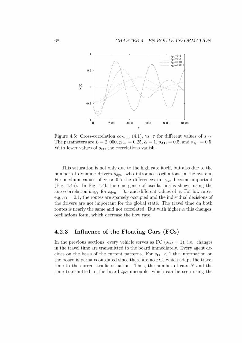
There are some innovative technologies, which foster the development ofITS, e.g., GPS, GSM, Internet. The Global Positioning System (GPS) isimportant since it allows for locating an object using at least three satellites.The Internet offers huge possibilities for distributing information. In future,it will be available on in-vehicle devices. Nowadays, a lot of web-pages alreadyoffer real-time information about the traffic situation to the user1.

1.1.4 Temporal Nature of Information

Since the idea of ITS is to provide information, the temporal nature of thedata as well as its use in traffic scenarios should be discussed briefly. Con-ceptually, information may fall into three distinct temporal classes [25, 57]:

Historical Data

Historical or after-trip information [62] reflects the previous states of the net-work. It can be either objective (measured), or subjective (own experience).

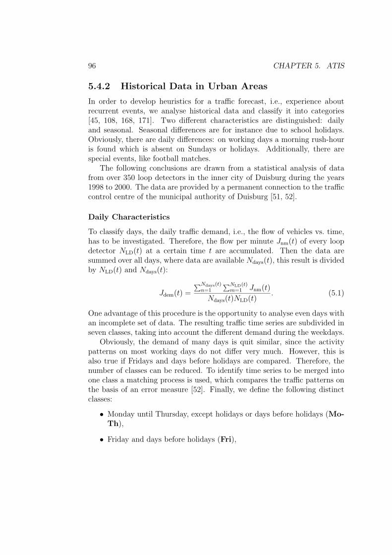
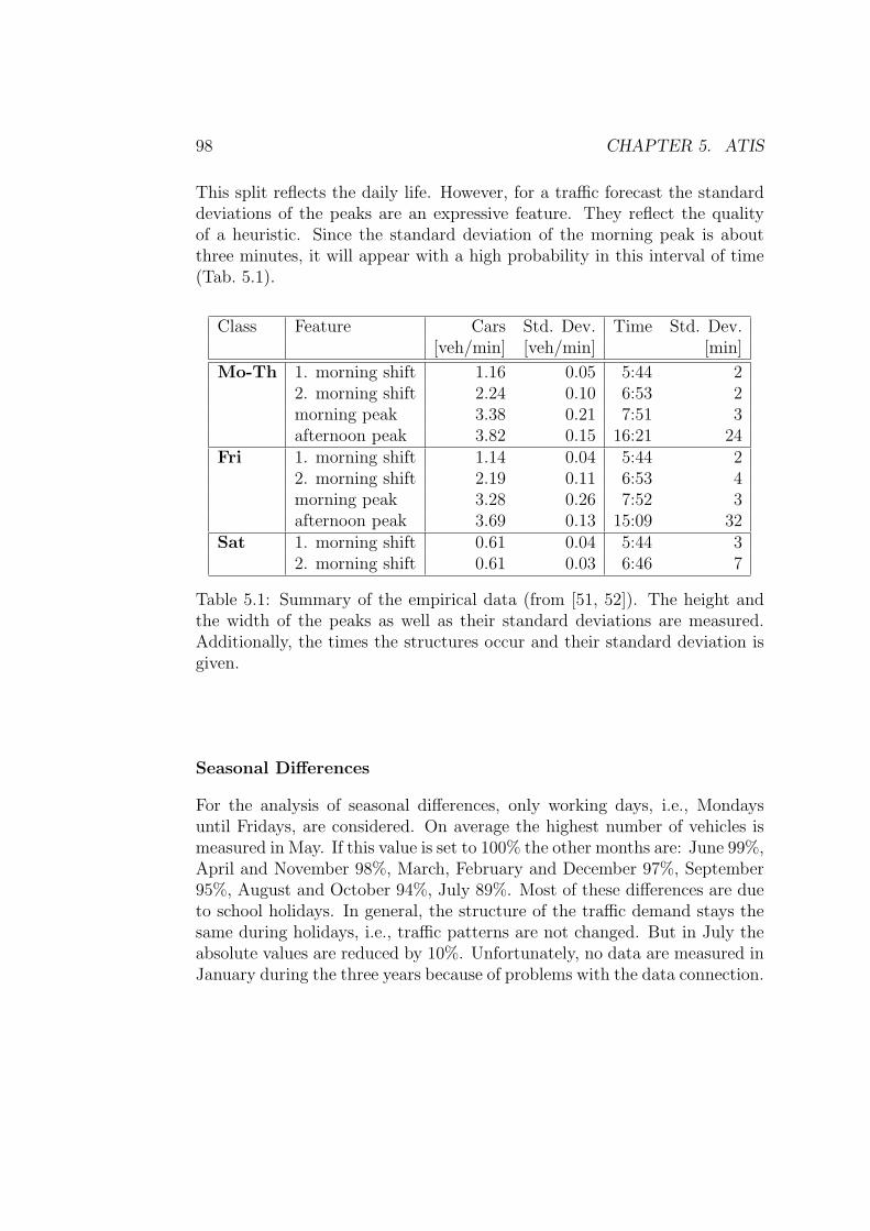
1See http://www.traffic.uni-duisburg.de/links/traf.html.

1.1. INTRODUCTION 9

The objective historical data are used to categorise daily traffic demandsand extract heuristics [45, 52, 108, 168, 171], which can be used for a trafficforecast (see Sect. 5.4.1).

Current Data

Current information is provided real-time and should be the most up-to-date information. The basis are data measured by detection devices (seeSect. 1.1.2).

Predictive Data

This kind of data reflects the expected traffic conditions. The predictiveinformation can be short-term, up to one hour, or long-term, up to one day.To provide such data, intelligent algorithms are needed to combine historicaland predictive data (for details Sect. 5.4).

1.1.5 Information in Traffic Systems

All temporal classes of data are provided before a trip or during the trip:

Pre-Trip Information

These data are transmitted, e.g., via the Internet or GSM. Since the roaduser has time to analyse and process it, the amount of information can behigher than for en-route systems. This kind of information introduces day-to-day dynamics of the route choice behaviour into traffic systems (for detailsee Chapter 3).

En-Route Information

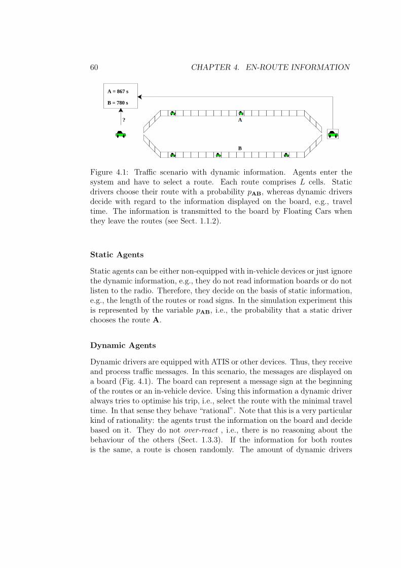
In order to support the road user during his trip data are transmitted en-route or on-trip. Possible modes of transmission are Variable Message Signs(VMS) or radio broadcast. Therefore, the content and amount of informa-tion can vary strongly. In general, it should be short and concise. In contrastto pre-trip, en-route information leads to within day-dynamics of the routechoice behaviour (for details see Chapter 4).


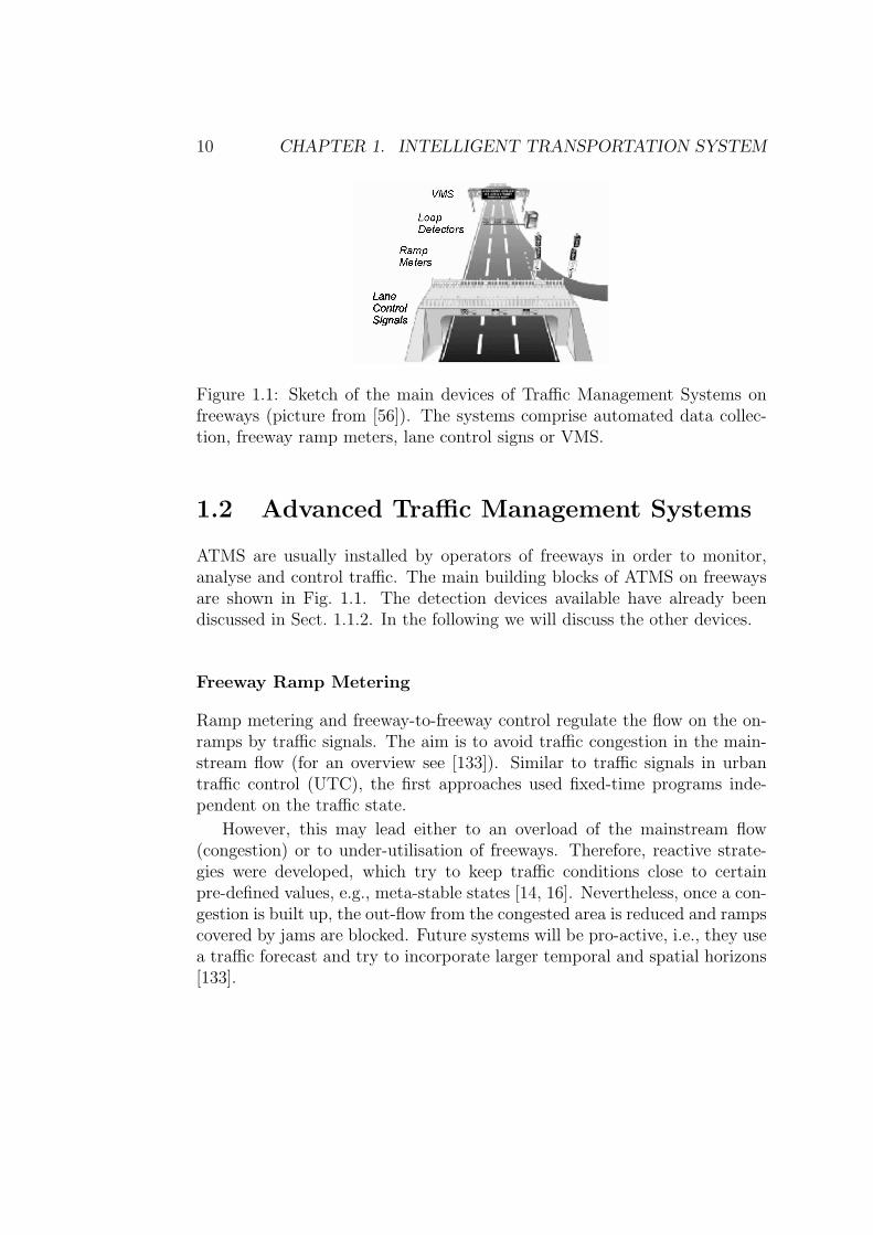
Figure 1.1: Sketch of the main devices of Traffic Management Systems onfreeways (picture from [56]). The systems comprise automated data collec-tion, freeway ramp meters, lane control signs or VMS.

1.2 Advanced Traffic Management Systems

ATMS are usually installed by operators of freeways in order to monitor,analyse and control traffic. The main building blocks of ATMS on freewaysare shown in Fig. 1.1. The detection devices available have already beendiscussed in Sect. 1.1.2. In the following we will discuss the other devices.

Freeway Ramp Metering

Ramp metering and freeway-to-freeway control regulate the flow on the on-ramps by traffic signals. The aim is to avoid traffic congestion in the main-stream flow (for an overview see [133]). Similar to traffic signals in urbantraffic control (UTC), the first approaches used fixed-time programs inde-pendent on the traffic state.

However, this may lead either to an overload of the mainstream flow(congestion) or to under-utilisation of freeways. Therefore, reactive strate-gies were developed, which try to keep traffic conditions close to certainpre-defined values, e.g., meta-stable states [14, 16]. Nevertheless, once a con-gestion is built up, the out-flow from the congested area is reduced and rampscovered by jams are blocked. Future systems will be pro-active, i.e., they usea traffic forecast and try to incorporate larger temporal and spatial horizons[133].

1.3. ADVANCED TRAVELLER INFORMATION SYSTEMS 11

Variable Message Signs

VMS are used to set speed limits or to display information to the road user. Indifferent countries the amount of information displayed on these devices varya lot: In Germany, most VMS do not present recommendations, e.g., traveltime, but only road signs. In other European countries, like the Netherlands,Great Britain or France, travel times and recommendations are given [34,64, 70, 166]. Additionally to VMS, lane control signals are employed whichallow for a traffic responsive use of lanes.

Urban Traffic Control (UTC)

In contrast to freeway traffic control, UTC concentrates on traffic signals andtheir coordination. Different solutions to traffic signal coordination whichmake use of multi-agent systems are presented in Sect. 2.2.2.

However, most of the control strategies are implemented independently,thus they fail to exploit the synergistic effects that might result from a co-ordination of the respective control actions. Therefore, an advanced conceptfor integrated freeway network control should not only coordinate these mea-sures but also include information systems, e.g., route guidance.

1.3 Advanced Traveller Information Systems

An integral part of ITS are ATIS [1, 13, 86, 87, 88], which provide real-time information about the traffic situation to travellers, e.g., travel times,location of incidents or weather conditions (see Chapter 5). Their aim isto alleviate traffic congestion and to ameliorate the capacity of the existinginfrastructure. The individual road user can benefit from such systems sinceanxiety and stress associated with navigating through the network are re-duced. Thus, there should be a significant overall reduction in travel time,delay and fuel consumption.

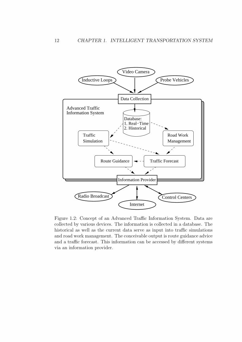
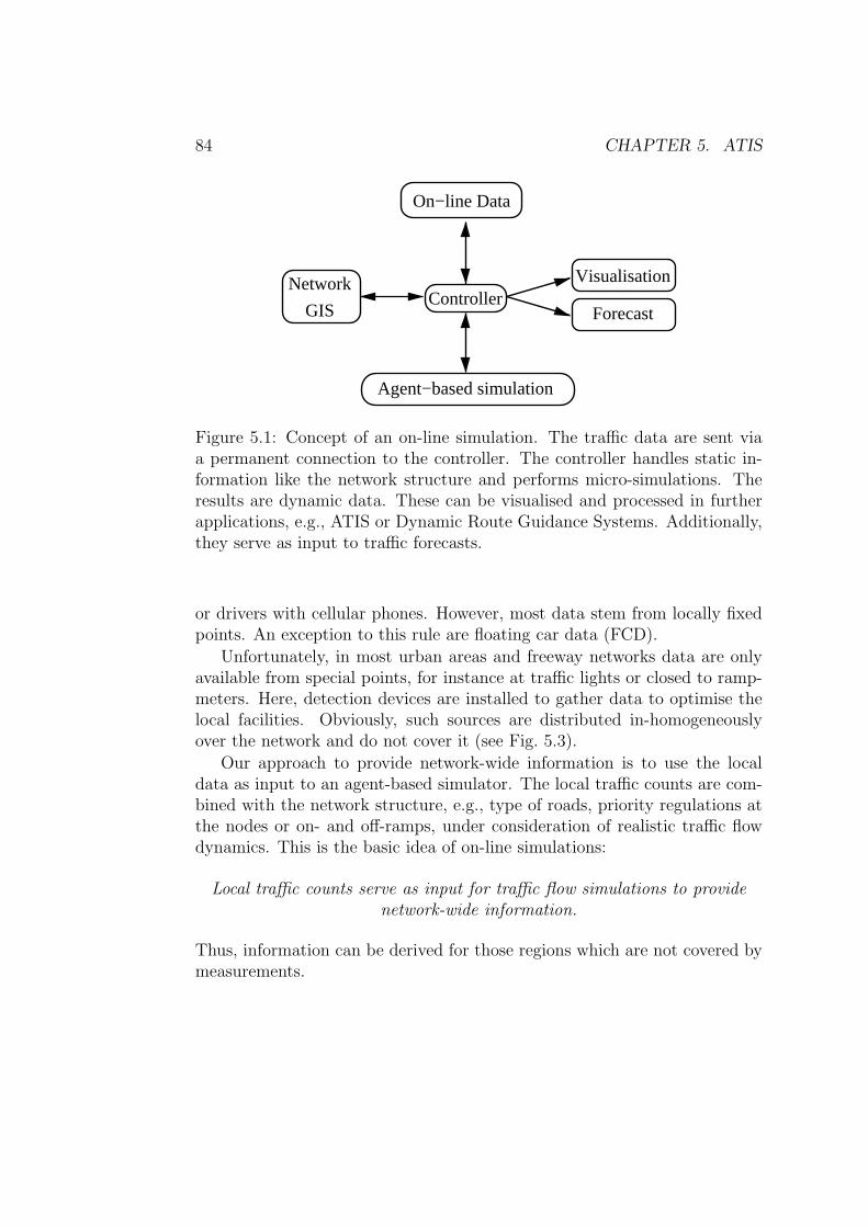
A concept of an ATIS is shown in Fig. 1.2. The input into the system areraw data stemming from various detection devices, discussed in Sect. 1.1.2.These are stored in a suitable database and processed using simulations. Theoutput of the process are dynamic data about the current traffic state, e.g.,link travel times or velocities, sometimes even predictive data are available.

Since the road user is only interested in a special part of the information,dynamic route guidance systems are used, which calculate the best route


Inductive Loops

Video Camera

Radio Broadcast

Internet

Control Centers

Probe Vehicles

Information SystemAdvanced Traffic

Route Guidance Traffic Forecast

Data Collection

1. Real−Time2. Historical

Database:

Information Provider

TrafficSimulation Management

Road Work

Figure 1.2: Concept of an Advanced Traffic Information System. Data arecollected by various devices. The information is collected in a database. Thehistorical as well as the current data serve as input into traffic simulationsand road work management. The conceivable output is route guidance adviceand a traffic forecast. This information can be accessed by different systemsvia an information provider.


with regard to different criteria, like travel time, distance, signals, comfort,or even scenic quality [32, 147, 159]. An ATIS based on an on-line simulationis presented in Chapter 5.

1.3.1 Possible Influences on Travel Behaviour

Information systems are only effective if they are able to convince the roaduser to change his behaviour. In principle, there are four different options:

Spatial

Nowadays, the strategy of most information systems is to change the spatialdistribution of traffic patterns, i.e., to provide route guidance. The idea is tooptimise the usage of the infrastructure by shifting traffic from saturated toemptier areas.

Temporal

Giving alternative routes is easier than recommending another departuretime since for such recommendations a (short-term) traffic forecast or ratheranticipatory route guidance is necessary (see [35, 36] and Sect. 5.4). Ina survey based on an information system in Paris, individuals were askedabout their willingness to change the behaviour after receiving information.1% was willing to cancel the trip, 2 % changed to another mode, 16 % toanother route and 23 % to another departure time [61]. Obviously, shiftingthe departure time especially during rush-hours may help to defuse thesetemporarily [147].

Modal Split

The main objective of most political programs today is to change the modalsplit, i.e., to distribute traffic among all means of transportation. However,one basic condition for a modal change is reliable information about timeta-bles and delays which would make public transportation more attractive [75].

Cancel Trip

Due to initiatives like tele-commuting programs and e-commerce, driversperhaps abandon their daily trips. However, most of the road users have


certain habits, and there has to be an incentive to change behaviour, likea shorter travel time or a more comfortable trip. Therefore, it is unlikelythat somebody abandons travel plans because they are connected with someutility (use or pleasure), e.g., enjoying the spare time.

1.3.2 Potential Benefits

In the previous sections, ITS and especially ATIS are discussed. Obviously,they have the potential to change the nature of public transport as well asprivate car travelling in a yet unknown way. Although the systems havereached a high technological level, their impact on the traffic patterns is notyet known.

Today, it is widely accepted that information systems offer enormouspotential for reducing delays and wasted mileage. The underlying assumptionbehind this belief is that in the current situation drivers do not have enoughreliable information and thus ignore the actual situation in the network. Onecould say:

The traffic problem is based on a lack of reliable information.

There are many studies that report a positive impact of ITS, e.g., a reductionof the overall travel time (for an overview see [32]). In [9] the experience ofa road work in Berlin is reported. Publishing the impairments due to theplanned construction in a newspaper, helped to alleviate the negative effects.

In general, two different situations can be distinguished: recurrent andnon-recurrent congestions [62, 63]. The former can be induced by persistentbottlenecks, e.g., permanent lacks of capacities during rush-hours, whereasthe latter are mostly due to unforeseen events, like accidents.

ITS offers a short-term benefit for non-recurrent congestion, since thedrivers are informed about day specific events. Recurrent obstructions aredifferent, since there is a learning process beyond these. The road users de-velop certain strategies to cope with such perturbations. In this case, ITSoffer a long-term benefit by changing the behaviour of, e.g., commuters orcommercial vehicles. Additionally, the systems are favourable for driverswhich are not familiar with the network, since they need and accept infor-mation to a much higher degree than road users who are familiar with theroad network [111].


1.3.3 Potential Drawbacks

The most important issue is of course the quality, reliability and availabilityof the traffic information. If the quality is not guaranteed or the informa-tion is not reliable nobody will follow route recommendations. Additionally,information has the potential to disturb or even destroy traffic patterns dueto the following behavioural phenomena [25]:

Over-Saturation

ITS can offer a huge amount of information to the user. But if people areconfronted with too much information, they are over-saturated and ignoreit [74]. Instead of following the advice, they develop simple heuristics to solvethe problem. Therefore, especially ATIS should offer personalised informa-tion [1, 147].

Over-Reaction

A more fundamental problem is the over-reaction, which occurs if too manydrivers respond to the information. Suddenly, a congestion may be trans-ferred from the original area to the alternative routes. People start to antic-ipate the behaviour of the other drivers’. This anticipation gets even worseif predictive information is given. It might cause oscillations of traffic flowamong the alternatives, since fast routes attract traffic and, in the process,are made slower, whereas the slower routes become faster [25, 84] (see alsoChapter 4). Therefore, it is inevitable to incorporate the behaviour of thedrivers in a forecast [35, 36, 160, 162].

Concentration

A set of drivers who go from one origin to one destination tend to use differ-ent routes, since they have different preferences or perceive the situation indifferent ways. This leads to a natural distribution among the routes.

Nevertheless, ATIS can reduce these variations if all the drivers use theobjective information transmitted. As a result a greater number of them mayselect the best alternative and consequently drivers with similar preferenceswill choose the same route, leading to congestion on this [5, 161].

Although the effect of over-reaction and concentration are similar, thenature of both phenomena is different [25]. Concentration is intrinsic to


many information systems, whereas over-reaction is a consequence of thefact that divers cannot forecast the behaviour of the others. Thus, there is alack of coordination (see Sect. 3.6 and Chapter 4).

1.4 Discussion

In this chapter Intelligent Transportation System (ITS) have been intro-duced. The objectives of these systems are to improve travel efficiency, en-hance the safety, provide economic benefits, conserve energy and protect theenvironment. In the six interlocking technology areas, there is a need for in-put data, provided by different detection devices, and advanced technologies,like GPS and the Internet.

In this paperwork, the focus is on Advanced Travel Management Systems(ATMS) and Advanced Traveller Information Systems (ATIS). The formermonitor and control traffic flow using, e.g., ramp meters or VMS. The aimof ATIS is to provide real-time information to the road user. The idea isto influence his behaviour in four different ways. Thus helping the driver tonavigate through the network easier.

Therefore, ATIS are thought to have an advantage for the road user.Nevertheless, the information provided can lead to over-saturation, over-reaction and concentration, which affect the traffic patterns in a negativeway. In order to convince the driver, the quality, accessibility and reliabilityof the information is crucial.

Besides, there are some policy issues, which need to be discussed, e.g.,the number of drivers to inform, as well as what kind of information shouldbe presented [25]. Other approaches try to regulate traffic by road pricing[56].

Nevertheless, while a lot of efforts have been directed toward technologicalaspects, little theoretical work has been done to investigate the impact ofinformation in traffic systems. Therefore, in this thesis special attention ispaid to the effect of concentration and over-reaction.

Chapter 2

Agents in the Traffic Domain

In general, traffic systems, like urban traffic or pedestrian crowds, consistof many autonomous, intelligent entities, which are distributed over a largearea and interact with each other to achieve certain goals. However, theseentities may represent completely different things, like traffic lights, trucksor even road users. For instance in an urban traffic scenario, traffic lightsand control centres can negotiate the best signal plan for a road network.

A powerful method to describe such systems are multi-agent models, sincethey offer a simple, intuitive way to describe every autonomous entity on theindividual level. This chapter aims at giving insight into the concept ofagents. The basic notions are introduced and discussed. Additionally, differ-ent applications of multi-agent systems to the traffic domain are presented.For instance the distributed problem solving in traditional scheduling prob-lems in air, railroad and road traffic, or autonomous systems to monitor andcontrol urban traffic control are discussed. Special attention is paid to trafficflow models which describe drivers´ behaviour not only on a reactive but alsoon a cognitive level.

2.1 Basic Concepts

The expression “agent” originates from the Latin word “agere”, or “to do”.Hence, one may see an agent as anything that acts. In recent years, theconcept of an agent has become popular in many research areas, like com-puter science [169], sociology [101], economics [113] or even physics [117].Depending on the application area the term agent can have many different

17

18 CHAPTER 2. AGENTS IN THE TRAFFIC DOMAIN

meanings. For instance in economics, an agent is a person which acts onbehalf of another person.

In the following sections, the basic concepts established in the field of arti-ficial intelligence are discussed. In order to identify natural agent systems, itis important to ask: what are the basic properties of an agent? Additionally,agents exist in a certain environment, which also has some basic properties.For the implementation the concrete type of agent and its architecture areimportant. Going from a single agent to a multi-agent system, communica-tion or cooperation between the different entities becomes important.

2.1.1 What is an Agent?

Giving a precise answer to this question is far beyond the scope of thispaperwork. No general definition of an agent exists. An agent can representan autonomous entity which is situated in an environment and interacts withit and the other agents to achieve specific goals (for an overview see [120,141, 169]). These entities can be very different depending on the scenariosdescribed, e.g., actors in a simulation of societies in contrast to so-calledsoftware agents, i.e., systems which are placed in an software environment,like the Internet.

Since there is no general definition it can be very helpful to describe themost important properties of an agent [101, 169]. An agent is:

• Situated.Every agent is situated in an environment. It perceives information viasensors and acts on the environment via effectors [141]. The definitionof the environment depends on the application (see next section).

• Reactive.Changes in the environment are recognised by the agent and the be-haviour is modified in time. Therefore, its behaviour is flexible, i.e.,the actions are not predefined but depending on the situation.

• Autonomous.This means that the agent is self-determining and decides about hisactions only with regard to its perceptions and the internal knowledge.

• Social.The agent interacts and communicates with other agents. The social

2.1. BASIC CONCEPTS 19

contact is essential in order to coordinate behaviour, achieve commonplans or solve problems cooperatively.

• Rational.Every agent is committed to its goals. This is very important since thebehaviour should be more than pure reaction to the environment. Theagent should even be able to show an initiative because of an internalmotivation.

2.1.2 Environment

As discussed in the previous section, every agent is situated in an environ-ment, which also has some basic properties: accessible, determined, relevanceof history, dynamic and discrete. In the following, we discuss these differentaspects since they are crucial for the design of a multi-agent system [141].The environment should be:

• Accessible.What information about the environment is accessible to the agent?Such a question is strongly related to the knowledge the agent mayhave.

• Determined.To what extent is the next state of the environment determined bythe actions of the agent? This question is important because theagent needs to know about its impact on the environment.

• Relevance of History.Does the future state of the environment depend on the history ofthe system? The relevance of history determines the importance of amemory for an agent.

• Dynamic.Are there changes in the environment while the agent is selecting anaction? If this is the case there is the requirement to operate in real-time, which has an impact on the design of the system.

• Discrete.Are perceptions within a range of discrete values or are there actions


which require a continuous set of parameters? In many applicationsspace and time are discrete, e.g., a grid of cells or time steps [102, 126].

2.1.3 Types of Agents

In the previous sections, the important ingredients for the design of anagent have been discussed. For the implementation an agent architectureis necessary. However, in the literature types of agents and architectures areclassified in many ways and the reader is referred to, e.g., [120].

Basically, two basic kinds of agents can be identified: reactive and cogni-tive agents. A reactive agent only maps possible perceptions to the availablereactions, e.g., stimulus-response systems. Such simple behaviour is oftenused in car-following models (see [37] and references therein). The cognitiveor deliberate agent is endowed with reasoning capabilities.

In order to model complex behaviour, it is helpful to distinguish differenttypes of behaviour. In the context of cognitive engineering, the followingthree hierarchical classes are proposed [136]:

• Skill-Based.This behaviour refers to fully automated activities (perception – exe-cution), typically used in routine situations.

• Rule-Based.Rule-based behaviour corresponds to stereotyped actions (perception –situation recognition – planning – execution).

• Knowledge-Based.This behaviour is the most complex. It describes conscious activities,involving problem solving and decision making (perception – situationrecognition – decision making – planning – execution).

In this scheme, reactive agents show skill- or even rule-based behaviour. Aprominent example for deliberate architectures is BDI: belief, desire, inten-tion (see [135] and references therein). In the BDI theory, an agent has threeinternal parameters: beliefs, desires and intentions. The beliefs contain thecurrent knowledge about the environment and the impact of its actions. Thiscan be information gathered by previous experience. The desires describe allgoals of an agent, whereas the intentions are generated from reasoning aboutthe current beliefs and goals. They determine the best possible action in thecurrent situation.

2.1. BASIC CONCEPTS 21

2.1.4 Multi-Agent Systems

A system of interacting agents is called a multi-agent system. In such systemsadditional properties can be identified which go beyond the properties ofa single agent. These characteristics can help to identify “natural” agent-systems. The following general properties are defined in [89]:

• Every agent has only a limited view of the whole system, i.e., it hasincomplete information or capabilities to solve problems.

• Therefore, the data is kept local, i.e., the internal status of the agent isnot known to all other agents.

• In the ideal case the agents act in an asynchronous manner, i.e., anupdate may be in parallel.

• There is no central control system, which governs all agents. This isalso only true in an ideal case.

The last property holds only for a few systems, like drivers in a road net-work. Especially, in systems with distributed problem solvers, it may benecessary to have a central control, which resolves conflicts between agentswith different goals.

One important issue in multi-agent systems is the communication andthe cooperation between the different agents, since these interactions formthe basis for coherent behaviour. There are already a lot of concepts andstandards for communication and cooperation in multi-agent systems, whichare very promising and can also be applied to the transportation domain[76, 132].

2.1.5 Cooperation and Coordination

In a society of loosely-coupled agents, where each has limited knowledgeand expertise, cooperation and coordination are necessary to achieve a com-mon goal which is beyond the individual capabilities. Note that cooperationmeans sharing a common goal, whereas coordination is the process of takingthe plans of others into account. There are many different mechanisms forthe coordination among agents, e.g., contract-net protocol or negotiation.


Contract-Net Protocol

The contract-net protocol is one of the earliest proposals for a protocol ofcoordination. The main objective is to provide a framework to allocate tasksamong a network of nodes or agents. The process is initiated by a managernode sending information to contractor nodes in form of announcements. Thecontractor nodes which are idle react to the announcement by evaluating itwith regard to their own interest, expertise, and availability of resources.If the announcement is regarded as interesting a bid message is sent backin order to place a contract. The manager evaluates all bids received andawards the task to the most suitable node. This protocol is ideal for logisticschains, e.g., in [154] an application has been investigated, where the networkshould track vehicles over a large geographical area. Note that the protocolguarantees a solution but not an optimal one.

Peer-To-Peer Negotiation

In contrast to the contract-net protocol, peer-to-peer negotiation denotes atwo-way communication in which the interested parties exchange informa-tion and come to an agreement. The process involves two main steps: i)identification of the potential communication partner and ii) modification ofthe intentions of these agents to avoid harmful interactions or initiate co-operation. The majority of these interactions are due to the appearance ofconflicts. In [165] a strategy for settling conflicts among a group of agents inthe domain of air traffic control is developed. In the following, applicationsof the basic concepts to the traffic domain are described.

2.2 Applications

2.2.1 Scheduling Problems

The traffic domain is full of complex systems, where the solution process canbe based on agents since the objects can be naturally identified as agents,e.g., air traffic control, transportation planning and scheduling or road trafficcontrol [121]. In many of these applications the question arises, how differentautonomous entities can work together effectively to achieve a common goal.This question is typical in the field of distributed problem solving (DPS).The main objective is to find a decomposition of a complex problem and an

2.2. APPLICATIONS 23

allocation of tasks among a group of problem-solvers in a way in which theydo better as a group than on their own.

Air Traffic Control

On the one hand, the major aim in air traffic control is to guarantee andeven improve the safety of the whole system. On the other hand, intelligentaircraft/airspace systems (IAAS) try to ensure that the demand for air trafficis met, with fewer restrictions, fewer delays. In a simple approach, two kindsof agents are identified: aircraft and management agents [165]. The man-agement system monitors and controls traffic flow. Each aircraft agent alsoobserves the situation and constructs a plan to reach the destination as fast aspossible under the constraint to keep an appropriate distance from the otherplanes. The conflicts that occur if two agents come too close, are resolved bynegotiation, i.e., peer-to-peer communication (see Sect. 2.1.5).

Transport Planning

Because of their inherent distributed nature, the dynamics and uncertaintyin the setting, transport planning and control are highly promising areas formulti-agent technologies. In general, incoming transportation orders have tobe distributed among different transport vehicles, means of transportation,or routes. Sometimes even the orders have to be reorganised, i.e., to be splitand put together in a new manageable way. Thus, vehicles, transport modesor routes are natural candidates for agents [41].

In order to tackle this problem, the MARS system is proposed: a multi-agent system where the transport companies are identified as cooperatingagents which have only limited, local resources [71]. Their task is to dividethe orders in sub-tasks and to distribute them among themselves. This isdone using local heuristics and contract-net protocols (see Sect. 2.1.5).

A system which even allows for an on-line dispatching, i.e., re-planningat run-time is TELETRUCK [41]. This approach uses so-called holonicagents. A holonic agent is a team of agents that commit themselves tocooperate, i.e., work toward a common goal. Additionally, they appear likean individual, coherent agent to the rest of the system. This structure allowsfor a more flexible resource management in the planning process. The multi-agent system approach goes beyond the classical operations research (OR)algorithms, since these have to be restarted if the plan is modified or adapted.


The planning process is implemented with an incremental anytime algo-rithm, i.e., an algorithm that starts with a sub-optimal solution and is capableof optimising the solution as well as integrating new tasks in the on-goingplanning and execution process. A first solution is found via executing acontract-net protocol for forming the holonic agents and assigning the tasks.Since there is no guarantee for an optimal solution, special attention is paidto the optimisation using the so-called simulated trading approach [31, 110].The idea of this approach is to plan by negotiating about exchange of tasksor parts of holonic agents.

Railroad Traffic

For the solution and optimisation of the corresponding problem in railroadtraffic Lind and Fischer propose a multi-agent system [31, 110], which com-prises small modules, like the Cargo-Sprinter. In their approach, the modulesare identified as agents. They show that an organisation of trains in smallmodules is very efficient. The algorithms are similar to the TELETRUCKapproach, i.e., they also use an incremental anytime algorithm and simulatedtrading for on-line scheduling. The presented results are quite promising.

Multi-Modal Solutions

Nevertheless, in the future multi-modal transport planning systems have tobe developed. Besides suitable theoretical concepts, the main drawback isthe availability of data from the different modes of transportation.

2.2.2 Urban Traffic Control

In Chapter 1 Intelligent Transportation System are discussed. Some of themfollow the strategy to control traffic flow by means of signals, ramp metering[133] or Variable Message Signs (VMS) [70, 166]. The main objectives ofthese systems are to maximise the overall capacity of the network and tominimise travel times and energy consumption.

Traffic Signal Coordination

Especially, in urban areas where the road network is dense the dynamics arebasically governed by the traffic lights. However, it has been found that in

2.2. APPLICATIONS 25

urban traffic the patterns, e.g., rush-hours, are quite recurrent [52]. There-fore, a lot of traffic signal control methods are based on feedback algorithmsusing historical traffic demand data [27]. But the effectiveness of traffic con-trol system depends on its ability to react upon changes very fast. Therefore,a system should work in real-time, and should be autonomous, self-adaptiveand pro-active [138, 139]. Additionally, there is an inherent distribution offunctionality over the components. Thus, multi-agent systems become at-tractive to model such scenarios.

However, the basic question is how control is distributed over the agentsand how they communicate among themselves [17]. The first issue raises thequestion: are the elements autonomous or is there a certain hierarchy? Thesecond issue is connected to this question, because the more autonomousthe entities are the more communication is necessary. The optimisation ofa single intersection for instance does not necessarily imply that this localsolution is the system optimum. Therefore, coordination is a crucial point(see Sect. 2.1.5). In the following, different applications are presented totackle this problem.

In [18, 19, 20] a progressive signal system for urban areas is developed.Two setups are studied: in the first the lanes are identified as agents whichcompete for the green time. In the second approach, systems with agentsas intersections are studied. In both approaches special attention is paidto the coordination mechanism of the agents. This is done using two-waynegotiation about the best signal plan. In order to reduce the communication,an evolutionary game-theoretical approach with learning is applied.

Another approach is a framework for an Integrated Dynamic Traffic Man-agement and Information (IDTMT) [138, 139]. The system comprises twokinds of agents, namely: Road Segment Agents (RSA) and Intelligent Traf-fic Signalling Agents (ITSA), which are associated with an intersection. Theformer monitor the traffic on a link and provide this information to the latter.The ITSA receive the information and make decisions on how to control theirintersections based on their goals. Conflicts with the adjacent intersectionsare resolved by authority agents. The agents are hierarchically organised andthe goal of the authority agent is the optimal global control strategy.


(a) (b)

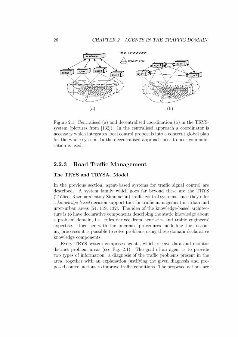
Figure 2.1: Centralised (a) and decentralised coordination (b) in the TRYS-system (pictures from [132]). In the centralised approach a coordinator isnecessary which integrates local control proposals into a coherent global planfor the whole system. In the decentralised approach peer-to-peer communi-cation is used.

2.2.3 Road Traffic Management

The TRYS and TRYSA2 Model

In the previous section, agent-based systems for traffic signal control aredescribed. A system family which goes far beyond these are the TRYS(Trafico, Razonamiento y Simulacion) traffic control systems, since they offera knowledge-based decision support tool for traffic management in urban andinter-urban areas [54, 119, 132]. The idea of the knowledge-based architec-ture is to have declarative components describing the static knowledge abouta problem domain, i.e., rules derived from heuristics and traffic engineers’expertise. Together with the inference procedures modelling the reason-ing processes it is possible to solve problems using these domain declarativeknowledge components.

Every TRYS system comprises agents, which receive data and monitordistinct problem areas (see Fig. 2.1). The goal of an agent is to providetwo types of information: a diagnosis of the traffic problems present in thearea, together with an explanation justifying the given diagnosis and pro-posed control actions to improve traffic conditions. The proposed actions are

2.3. DRIVER MODELS 27

derived by reasoning mechanisms. However, the key question is again theorganisation of the society of agents.

In the first TRYS-system a centralised approach is chosen (see Fig. 2.1a).Thus, there is a special coordinator agent, which endows knowledge on howto integrate local control proposals into a coherent global plan for the wholesystem [54]. However, the coordinator agent requires a lot of communicationand the system is not easily scalable. Therefore, the TRYSA2 has been devel-oped where the agents cooperate in a decentralised manner (see Fig. 2.1b).The coordination is done based on structural cooperation (for details see[132]).

The TRYS systems offer a good opportunity to demonstrate the effective-ness of multi-agent systems as well as their potential applications. Togetherwith the Municipal Authorities, the systems have been applied to the citiesof Barcelona, Madrid and Seville.

2.3 Driver Models

Up to now, we have seen that multi-agent systems are ideal in scenarios withan inherent distribution of functionality, especially when the cooperationbetween different entities is necessary to achieve a certain common goal, likein traffic control.

However, traffic can be viewed as a non-cooperative game between thetraffic authorities and the road users [48]. The former want to control trafficand achieve a system optimum (SO), i.e., a more efficient use of the capacities.The latter aim at optimising their personal travel time, i.e., user equilibrium(UE) [167]. In order to describe these games, the components of the trafficcontrol systems as well as the road users should be modelled as agents.

A fundamental problem is the different nature of the involved entities.The technical components are based on algorithms, like rule-based systems orfuzzy controllers, which can be implemented as agents very easily. But roadusers represent human beings and modelling human behaviour is very de-manding. In the following subsections, different multi-agent systems, whichdescribe the various aspects of road users´ behaviour, will be presented. Thestarting point for this discussion is the fundamental question, whether roadusers can be interpreted as agents.


2.3.1 Is a Road User an Agent?

Intuitively, it is obvious that every driver1 can be represented by an agent.In Sect. 2.1 we have pointed out that the basic attributes of an agent are:autonomous, situated, reactive, social, and rational.

The concept of an agent is well suited for the description of road users intraffic scenarios, because the drivers are autonomous entities which are situ-ated in an environment, adapt their behaviour to the dynamics they perceive(reactive), interact with other agents (social) in order to achieve a specificgoal (rational). The road user permanently perceives information via sensors,then analyses it, makes a decision and acts on the environment via effector.However, this insight is not completely new, but it offers an alternative in-terpretation of classical traffic flow models as well as a development of moregeneral and effective frameworks to model driver´s behaviour on a cognitivelevel.

2.3.2 Classical Traffic Flow Models

In general, classical traffic flow models describe the act of driving on a road,i.e., the perception and reaction of a driver on a short time-scale. This be-haviour is skill- or rule-based (see Sect. 2.1.3). Basically, there are two differ-ent approaches to model traffic, namely the macroscopic and the microscopic(for an overview see [50]). In the former a “coarse-grained” fluid-dynamicaldescription is used. Traffic is viewed as a fluid formed by the vehicles. How-ever, these vehicles do not appear explicitly in the theory and it is not possibleto individualise behaviour.

In contrast to that, microscopic models of vehicular traffic focus on indi-vidual vehicles. They are the basic entities and their behaviour is describedusing several different types of mathematical formulations. Car-Followingmodels for instance describe the motion of the vehicle, based on the basicprinciples of classical Newtonian dynamics (for an overview see [37]). Inparticle-hopping models the environment is subdivided in cells, i.e., discrete.This is done using the language of cellular automata (CA).

Nevertheless, any microscopic traffic flow model can be interpreted as a

1Note that throughout this work, the terms vehicle or driver are used to describe thedriver-vehicle object (DVO). However, a distinction is only made in “sub-microscopic”models, where the behaviour of driver within the car is described explicitly, e.g., PELOPS[164].


3 1

22

2

gap=2

cell length 7.5m

gap =3gap =1

velocity

s p

2

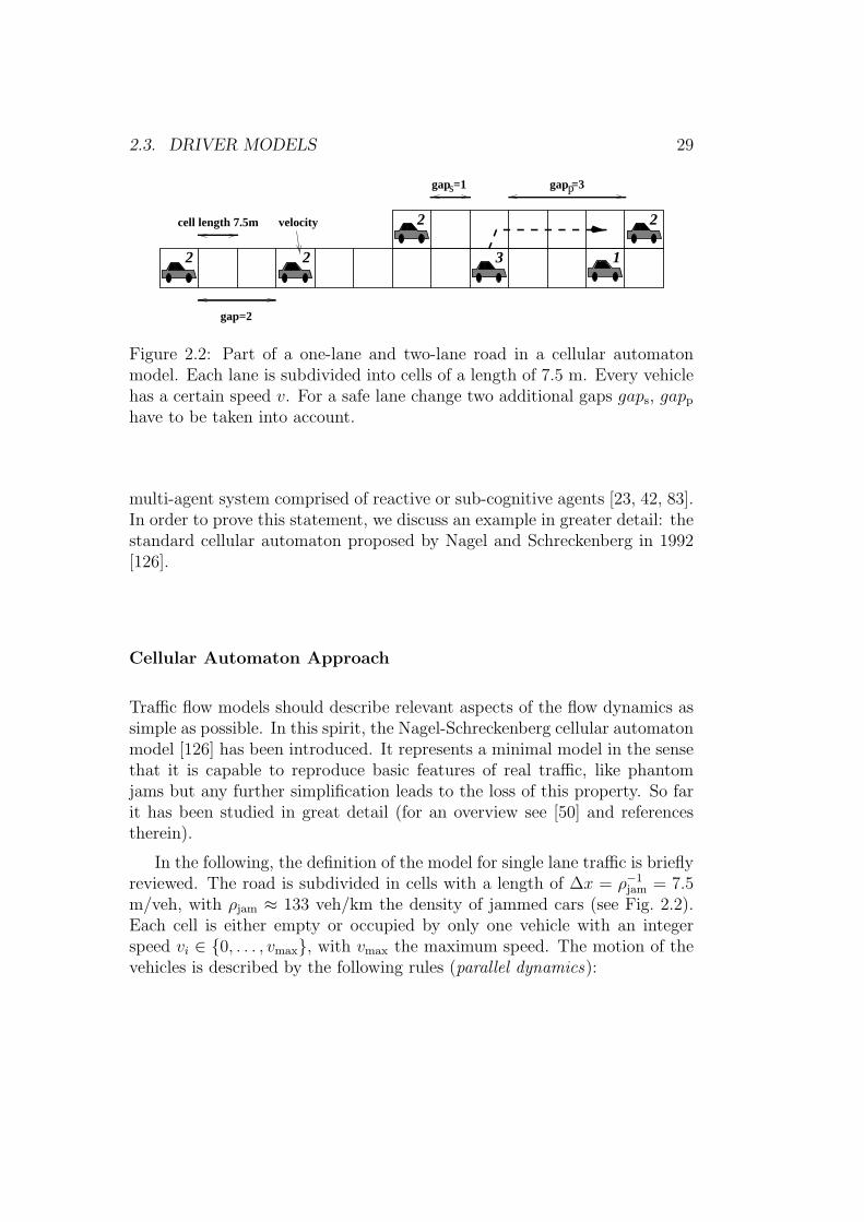
Figure 2.2: Part of a one-lane and two-lane road in a cellular automatonmodel. Each lane is subdivided into cells of a length of 7.5 m. Every vehiclehas a certain speed v. For a safe lane change two additional gaps gaps, gapp

have to be taken into account.

multi-agent system comprised of reactive or sub-cognitive agents [23, 42, 83].In order to prove this statement, we discuss an example in greater detail: thestandard cellular automaton proposed by Nagel and Schreckenberg in 1992[126].

Cellular Automaton Approach

Traffic flow models should describe relevant aspects of the flow dynamics assimple as possible. In this spirit, the Nagel-Schreckenberg cellular automatonmodel [126] has been introduced. It represents a minimal model in the sensethat it is capable to reproduce basic features of real traffic, like phantomjams but any further simplification leads to the loss of this property. So farit has been studied in great detail (for an overview see [50] and referencestherein).

In the following, the definition of the model for single lane traffic is brieflyreviewed. The road is subdivided in cells with a length of ∆x = ρ−1

jam = 7.5m/veh, with ρjam ≈ 133 veh/km the density of jammed cars (see Fig. 2.2).Each cell is either empty or occupied by only one vehicle with an integerspeed vi ∈ {0, . . . , vmax}, with vmax the maximum speed. The motion of thevehicles is described by the following rules (parallel dynamics):


R1 Acceleration: v′i ← min(vi + 1, vmax),

R2 Deceleration to avoid accidents: v′′i ← min(v′i, gapi),

R3 Randomising: with a certain probability pdec

do v′′′i ← max(v′′i − 1, 0),

R4 Movement: xi ← xi + v′′′i .

The variable gapi denotes the number of empty cells in front of the vehicleat cell i. A time-step corresponds to ∆t ≈ 1 sec, the typical reaction time ofa driver.

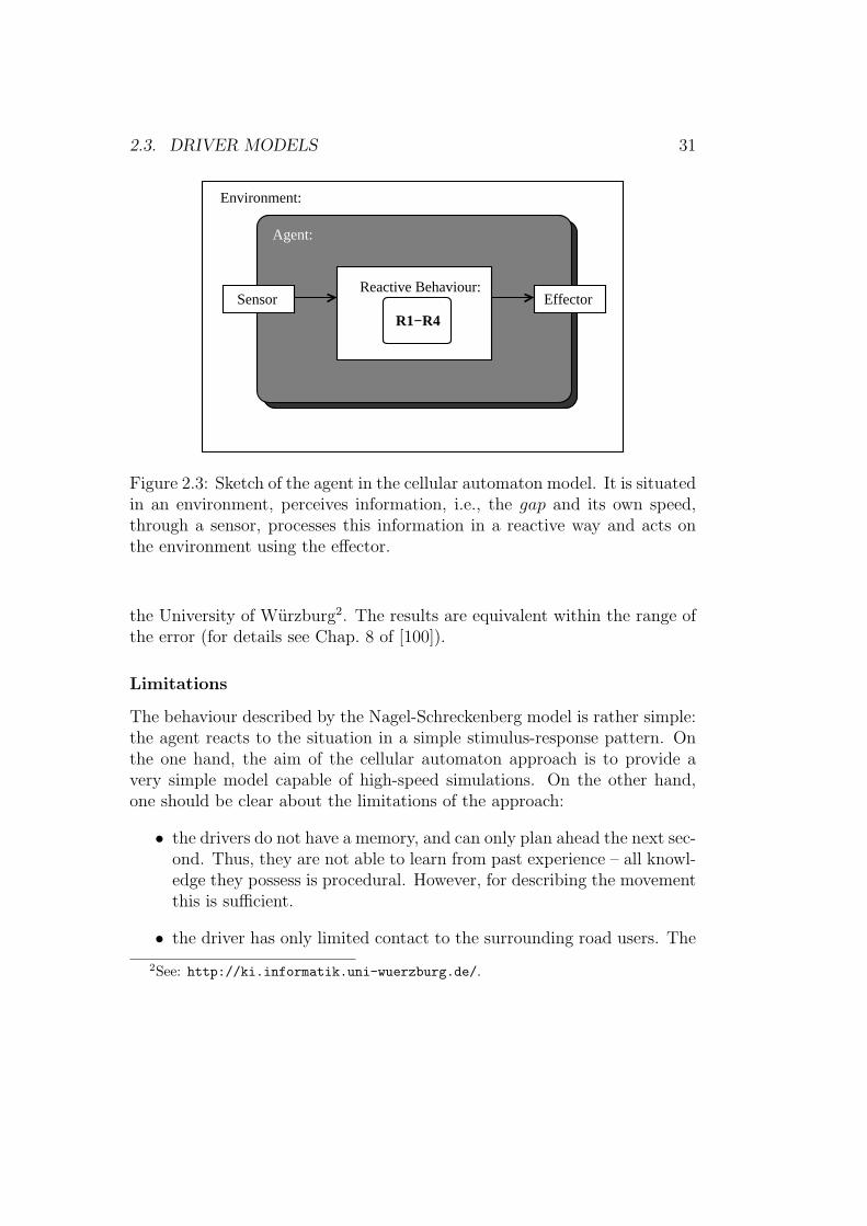
Every driver described by the Nagel-Schreckenberg model is a reactiveagent. He is autonomous, situated in a discrete environment (see Fig. 2.2),and has internal characteristics: its maximum speed vmax, and the decelera-tion probability pdec. During the process of driving, he perceives information,the distance to the predecessor gap and his own current speed v (Fig. 2.3).This information is processed using the four rules (R1-R4).

The first rule describes one goal of the agent, the driver wants to move atmaximum speed vmax. The other goal is to drive safe, i.e., not to collide withits predecessor (R2). In this rule the road user assumes that its predecessorcan brake to zero speed. However, this is a very crude approximation of theperception of an agent.

The first two rules describe deterministic behaviour, i.e., the stationarystate of the system is determined by the initial conditions. But drivers donot react in this optimal way: they vary their driving behaviour without anyobvious reasons. This uncertainty in the behaviour is reflected by the brakingnoise pdec (R3). It mimics the complex interactions with the other agents,i.e., the overreaction in braking and the delayed reaction during acceleration.Finally, the last rule is carried out, the agent acts on the environment andmoves according to his current speed.

The discussion makes clear that the cellular automaton approach is a sub-cognitive or reactive agent (see Fig. 2.3). In general, every cellular automa-ton can be interpreted as a reactive agent. The crucial point is to leave thecell-oriented view of the CA and to identify the objects in the cells as individ-uals. In order to prove the validity of the concept, the Nagel-Schreckenbergmodel was re-implemented using the multi-agent environment SeSAm (Shellfor Simulated Multi-Agent Systems, [100, 101]). This was done in close col-laboration with F. Klugl from the group of applied artificial intelligence of


Effector

R1−R4

Sensor

Agent:

Environment:

Reactive Behaviour:

Figure 2.3: Sketch of the agent in the cellular automaton model. It is situatedin an environment, perceives information, i.e., the gap and its own speed,through a sensor, processes this information in a reactive way and acts onthe environment using the effector.

the University of Wurzburg2. The results are equivalent within the range ofthe error (for details see Chap. 8 of [100]).

Limitations

The behaviour described by the Nagel-Schreckenberg model is rather simple:the agent reacts to the situation in a simple stimulus-response pattern. Onthe one hand, the aim of the cellular automaton approach is to provide avery simple model capable of high-speed simulations. On the other hand,one should be clear about the limitations of the approach:

• the drivers do not have a memory, and can only plan ahead the next sec-ond. Thus, they are not able to learn from past experience – all knowl-edge they possess is procedural. However, for describing the movementthis is sufficient.

• the driver has only limited contact to the surrounding road users. The

2See: http://ki.informatik.uni-wuerzburg.de/.


vehicles are linked to their immediate leader and follower, i.e., thereis only nearest-neighbour interaction. However, this is a more seriousproblem, since it seems that for the evolution of dynamic phases, likesynchronised traffic flow and stop-and-go traffic, long-range interac-tions are crucial [95, 96, 97, 130]. Therefore, models where the driveranticipates the speed of the predecessor are introduced [103, 104, 129].

Lane-Change and Network Traffic

In order to describe more complex rule-based behaviour, like multi-lane traf-fic, merging regions, and traffic lights, the set of fundamental rules has tobe expanded [66, 127]. For instance, a lane change has to be carried outwith regard to safety aspects and legal constraints, which vary between dif-ferent countries. A schematic lane change is shown in Fig. 2.2. First, anagent checks if it is hindered by the predecessor on its own lane. This isfulfilled if gap < v. Then it has to take the gap to the successor gaps and tothe predecessor gapp on the alternative lane into account. If the gaps allowa safe change the vehicle moves to the other lane. A systematic approach fortwo-lane rules can be found in [127].

2.3.3 Requirements in Knowledge-Based Applications

Classical microscopic traffic flow models describe fully automated activities,i.e., skill- and rule-based behaviour. They are used for modelling and simu-lating vehicular motion in road networks, e.g., on-line simulations [66, 148].For more complex applications, it is inevitable to model the knowledge-basedbehaviour of the road users in addition. One example are frameworks fortransportation planning [40] and traffic assignment [140]. Another exampleare applications which estimate the impact of ITS [161].

Transportation Planning and Traffic Assignment

Transportation planning deals with the long-term evolution of transportationsystems, e.g., in metropolitan areas (TRANSIMS [124]). A typical questionis: will a freeway construction indeed alleviate congestion, or will it reorganisethe places where people live, work, and shop and deteriorate the situationby transferring congestion to other parts of the network?


Basically, these frameworks comprise a demand and a supply model. Inthe demand model, drivers are represented individually. For each individual,the daily departure time and route choices are generated on the basis of pasttravel cost experiences, the knowledge of the perceived network conditions,and activity plans (see below).

The demand generation describes the “plan making” of the individuals.For executing these plans the supply model is necessary, which is responsi-ble to move the vehicles through the network on the basis of a traffic flowmodel with regard to the routes determined in the demand model. The re-sulting network conditions and costs experienced by drivers are feeded backinto the demand. One iterates between demand and supply until a steadystate is reached [124]. Nevertheless, there is no a priori reason why thereshould be a steady state. Note that steady state refers to the comparisonfrom one iteration to the next, not a steady state across the time of the day.

Drivers in ITS Environment

ITS provide current or even predictive information about traffic states to theroad user. A key question in this work is:

What is the impact of ITS on the traffic patterns?

It is crucial to answer this question since it is on the one hand believedthat ITS systems will have the potential to alleviate traffic congestion andenhance the performance of the road network [1]. On the other hand, thebehaviour of the road users in the presence of information is hardly known(see Sect. 1.3.3).

The intelligent devices will provide a lot of information about link traveltimes, densities, or route guidance to the road user. Thus, the drivers have tocollect even more information and evaluate this with a higher frequency. Thisclearly indicates that, e.g., travellers’ route choice behaviour has to be takeninto account for the development and effectiveness ITS. Special attention tothis problem is paid in this work (see Chapter 3 and Chapter 4).

2.3.4 Cognitive Driver Models

In the previous section, it was pointed out that in complex applications thereis a need to model knowledge-based behaviour, like decision-making andinformation assimilation. In the following, different examples for multi-agent


systems, which are capable to describe flexible knowledge-based actions, arepresented.

Agent-Based Models with Activity Plans

The first step in traffic planning is generation of the demand. In [40] anagent-based approach to solve this problem motivated by social science isproposed. Every agent has certain activities, like going to work, shopping,which induce a certain demand. The scheduling of the activities is carriedout with regard to the evaluation of the utility. Every agent gets to knowthe environment and thus has, e.g., a subjective representation of the roadnetwork, which is constantly evolving in response to trips made. A similarapproach is presented in [140]. The basic framework is the assignment toolDRACULA (Dynamic Route Assignment Combining User Learning and mi-crosimulAtion). This tool focuses on the influence of ITS on the assignmentprocess.

A Modular Driver Model

A conceptual framework for modelling drivers’ behaviour is presented in [42].Every agent is characterised by its goals, resources, and behaviour. The goalsand resources are internal parameters and the behaviour is modelled usingan architecture, which comprises five modules: effectors, sensors, communi-cation, intention and cognition.

The effectors, sensors and communication modules make contact withthe outside world. The communication is two-way and can for instance bea connection to service providers [43]. The intention module represents theagent´s long-term goals, and the cognition is the “heart” of the agent. Itcomprises knowledge, a problem-solver and a cooperation component. Theproblem-solver evaluates the sensor data and selects among the possible ac-tions with respect to the intention. The cooperation component checks thereceived messages and prepares those to be sent. In [42] only a classical car-following model is implemented in this architecture. But, the architectureallows for implementing complex applications with communication.

2.4. TWO-LAYER ARCHITECTURE 35

2.4 Two-Layer Architecture

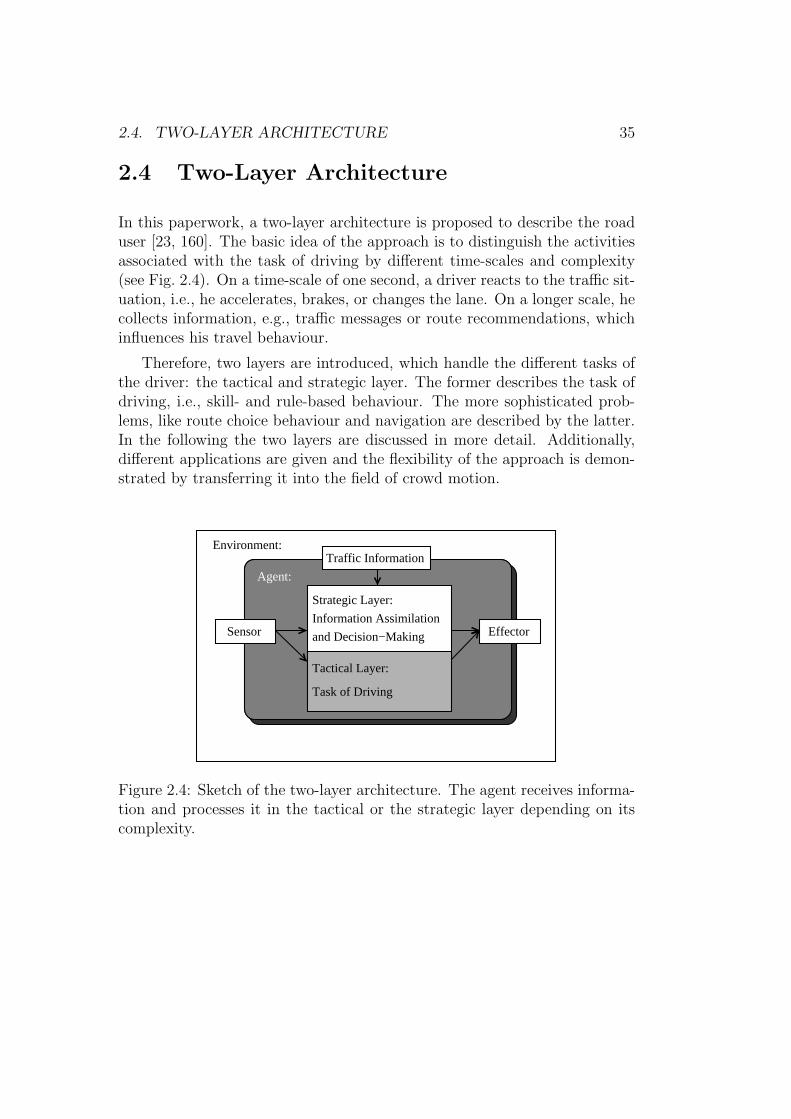
In this paperwork, a two-layer architecture is proposed to describe the roaduser [23, 160]. The basic idea of the approach is to distinguish the activitiesassociated with the task of driving by different time-scales and complexity(see Fig. 2.4). On a time-scale of one second, a driver reacts to the traffic sit-uation, i.e., he accelerates, brakes, or changes the lane. On a longer scale, hecollects information, e.g., traffic messages or route recommendations, whichinfluences his travel behaviour.

Therefore, two layers are introduced, which handle the different tasks ofthe driver: the tactical and strategic layer. The former describes the task ofdriving, i.e., skill- and rule-based behaviour. The more sophisticated prob-lems, like route choice behaviour and navigation are described by the latter.In the following the two layers are discussed in more detail. Additionally,different applications are given and the flexibility of the approach is demon-strated by transferring it into the field of crowd motion.

Effector

Traffic Information

Task of Driving

Tactical Layer:

Sensor

Agent:

Environment:

and Decision−Making

Information Assimilation

Strategic Layer:

Figure 2.4: Sketch of the two-layer architecture. The agent receives informa-tion and processes it in the tactical or the strategic layer depending on itscomplexity.


2.4.1 Tactical Layer

The tactical layer (see Fig. 2.4) describes the perception and reaction of thedriver-vehicle entity on a short time-scale of about one second, the typicalreaction time. The perceptions are received by the sensors. Based on themskill- and rule-based behaviour is shown, i.e., there are no cognitive elements.The whole structure is reactive or subcognitive. Especially, the followingaspects of the driving behaviour are modelled:

• accelerating and braking,

• anticipation,

• lane-changing processes,

• and merging behaviour.

In Sect. 2.3.2 it was pointed out that every microscopic traffic flow model canbe interpreted as a system of reactive agents. Therefore, the behaviour ofthis layer is modelled by a flow model. Throughout this thesis, the basicmodel used is the cellular automaton approach by Nagel and Schreckenberg[126].

2.4.2 Strategic Layer

The strategic layer extends the tactical one and is responsible for the in-formation assimilation and decision-making of a driver (Fig. 2.4). In theapplications described here, this layer is responsible for the following be-haviour:

• Information assimilation.Before and during a trip, a road user collects information in many way,for instance by radio broadcast or VMS. This information is processed,analysed, and is stored in the memory of the agent.

• Representation of the Road Network.Every road user owns a mental map about the environment or roadnetwork. This mental map alters permanently and is the basis for hisroute choice behaviour.


• Reaction to Traffic Messages and Recommendations.Every driver responds to traffic messages in an individual way. Hisreaction depends on his mental map and the stored information, butalso on his personal experience with the information, e.g., whether itis reliable or not.

However, in most models perfect rationality and utility maximisationis assumed. In real-world scenarios there is rarely an optimal solution tothe route choice problem available, since the process is highly dynamic anddepends on the behaviour of the others (see Chapter 4).

In this paperwork, we try to use several techniques to describe the strate-gic layer [21, 23, 161]. In general, the decision-making process in humanbeings is based not only on logical elements, but also involves some emo-tional components that are typically not considered. As a result, behaviourcan also be described by, e.g., the BDI-formalism (see Sect. 2.1.3). Basedon the categories of beliefs, desires or intentions, knowledge-based behaviourcan be formulated. A first implementation of a BDI-formalism in the contextof traffic assignment is proposed in [140].

Since the description of this layer is very demanding, a lot of researchwork has to be done in the future. In the following section the need for thislayer in the context of traffic forecast is discussed.

2.4.3 Case Study 1: Anticipatory Traffic Forecast

The prediction of traffic conditions is an integral component of many Ad-vanced Traveller Information Systems (Sect. 1.3). In general, real-time mea-surements are combined with other data, like historical time series, to gen-erate short-term forecast (see [11, 38, 45, 52, 57, 59, 99, 98, 107, 151, 168] amore detailed description of the different methods of traffic forecast are givenin Chapter 5).

However, the predictions are the basis of recommendations given to theroad user by means of communication such as Variable Message Signs orradio broadcasts. Each of these systems is confronted with a fundamentalproblem:

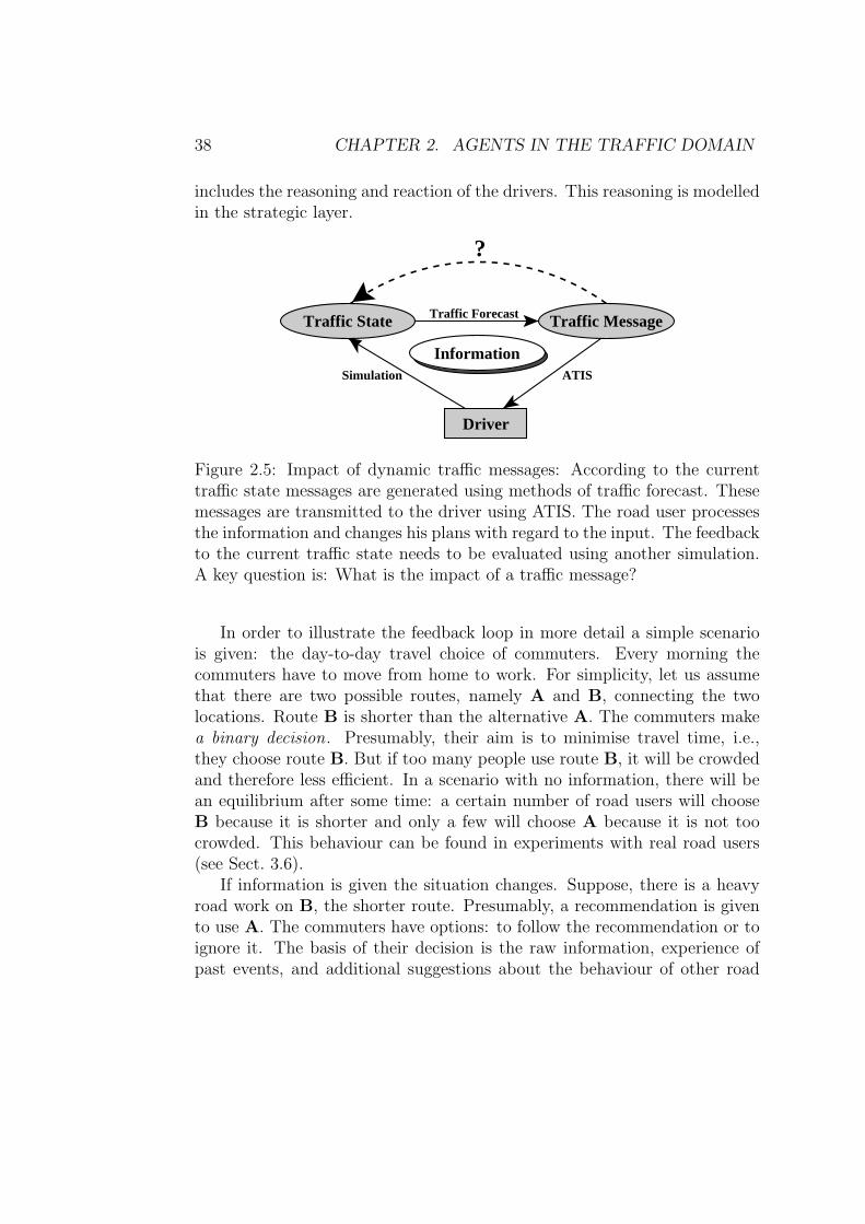
The messages are based on future predictions which themselves are affectedby drivers’ reactions to the messages they receive.

This leads to an undesirable feedback loop, as depicted in Fig. 2.5. Therefore,it is necessary to provide an anticipatory traffic forecast [35, 160], which


includes the reasoning and reaction of the drivers. This reasoning is modelledin the strategic layer.

Traffic State

ATIS

Traffic Forecast

?

Driver

InformationSimulation

Traffic Message

Figure 2.5: Impact of dynamic traffic messages: According to the currenttraffic state messages are generated using methods of traffic forecast. Thesemessages are transmitted to the driver using ATIS. The road user processesthe information and changes his plans with regard to the input. The feedbackto the current traffic state needs to be evaluated using another simulation.A key question is: What is the impact of a traffic message?

In order to illustrate the feedback loop in more detail a simple scenariois given: the day-to-day travel choice of commuters. Every morning thecommuters have to move from home to work. For simplicity, let us assumethat there are two possible routes, namely A and B, connecting the twolocations. Route B is shorter than the alternative A. The commuters makea binary decision. Presumably, their aim is to minimise travel time, i.e.,they choose route B. But if too many people use route B, it will be crowdedand therefore less efficient. In a scenario with no information, there will bean equilibrium after some time: a certain number of road users will chooseB because it is shorter and only a few will choose A because it is not toocrowded. This behaviour can be found in experiments with real road users(see Sect. 3.6).

If information is given the situation changes. Suppose, there is a heavyroad work on B, the shorter route. Presumably, a recommendation is givento use A. The commuters have options: to follow the recommendation or toignore it. The basis of their decision is the raw information, experience ofpast events, and additional suggestions about the behaviour of other road


users. With this collected information a simple decision-making process maybe based on the following consideration: if everyone follows the recommenda-tion, there might be no jam at all, thus it is better to use B. This behaviouris called overreaction [25].

However, the recommendation is based on the measurement/statisticsthat usually more drivers choose route B, thus a congestion might appearwhile the message is transmitted to the drivers, the basis of the formerlycorrect assumption about the traffic pattern is no longer true: the feedbackloop is closed. Such situations are found in many other systems, e.g., stockmarkets.

Today, the feedback in traffic systems is not very strong since the infor-mation is not precise enough. Once a road user has chosen a certain route,he will rarely be able to evaluate other alternatives. But reliable informationmight destabilise the system since it leads to situations where a contradic-tion between individual and collective aims occurs, a so-called social dilemma[26].

Here, different techniques will be used to model this behaviour. In thefollowing chapter, a two-route scenario is mapped on the Minority Game[46], a binary decision model. In Chapter 4 simulations are used to providedynamic traffic information in the same scenario. In Sect. 3.6, experimentscarried out with real road users are summarised.

2.4.4 Case Study 2: Application to Crowd Motion

Since the two-layer architecture presented above is very general, it can di-rectly be applied to model crowd motion. This is interesting since pedestriansare a crucial component in many transportation facilities. The applicationareas range from the analysis of traffic in simple hallways, where the flowis bi-directional, up to the description of the complex processes in airportsor shopping malls (for an overview see [79, 149]). In order to optimise thefacility design or to analyse evacuation processes, it is crucial to understandtheir behaviour as an individual and as a group.

The starting point of many modelling approaches in crowd motion areroad traffic flow models (e.g., [28, 29, 30]). Similar to road traffic, the modelsrange from macroscopic or gas-kinetic ones, to microscopic ones. The formerare based on the analogy to fluids or liquids. In the latter, pedestrians areidentified as basic entities. In the following, we restrict ourselves to themicroscopic models, especially those which are based on agents.


However, there are significant differences between the requirements formodelling road and pedestrian traffic. In road traffic, one finds flow restrictedto lanes, whereas pedestrian motion has more degrees of freedom. Since themotion is two-dimensional, special attention has to be paid to the the de-scription of way-finding behaviour. Moreover, pedestrians are self-propelledand their walking capabilities can vary widely. Every pedestrian is identifiedby a set of parameters, like age, gender or walking speeds, which are usuallydrawn from distributions [81, 82].

In general, a model should take into account different aspects of the mi-croscopic motion, like route choice behaviour or walking speeds, passing be-haviour, as well as macroscopic properties, such as formation of dynamiclanes and clusters, capacities of doors, escalators. Multi-agent systems offera flexible tool to model pedestrian traffic.

Effector

Tactical Layer:

Task of Walking

Sensor

Environment:

Strategic Layer:

Information Assimilation

and Wayfinding

Pedestrian:

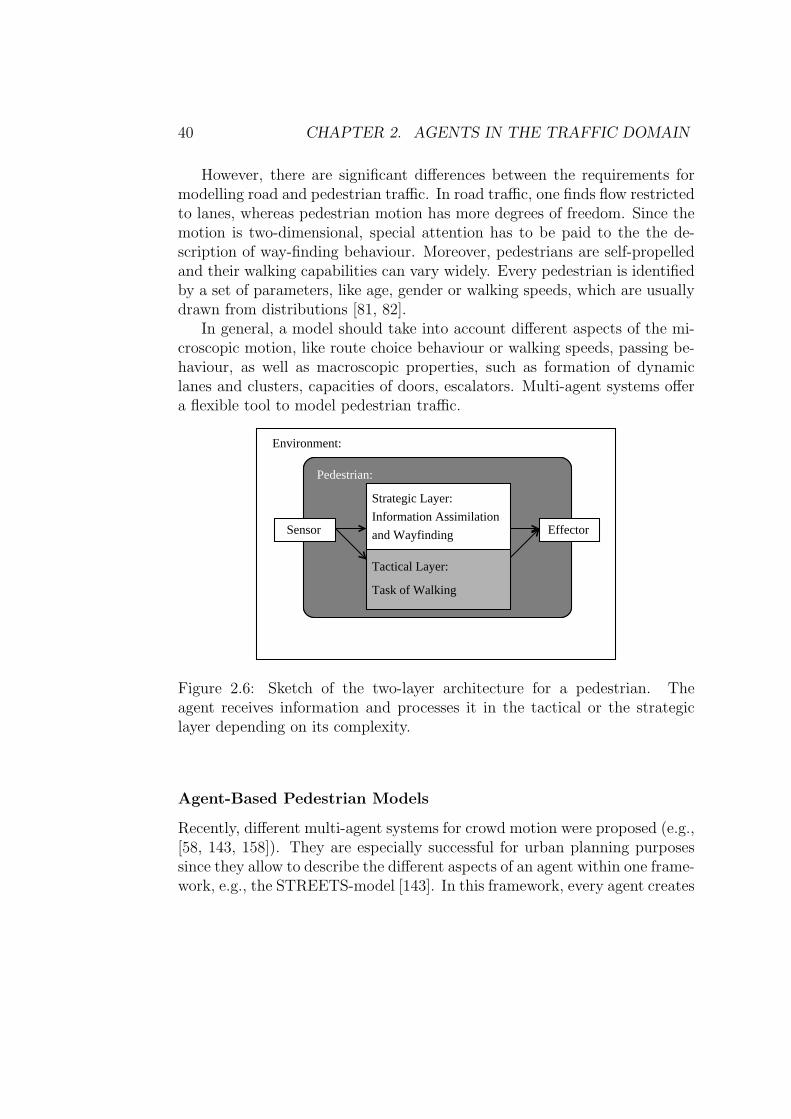
Figure 2.6: Sketch of the two-layer architecture for a pedestrian. Theagent receives information and processes it in the tactical or the strategiclayer depending on its complexity.

Agent-Based Pedestrian Models

Recently, different multi-agent systems for crowd motion were proposed (e.g.,[58, 143, 158]). They are especially successful for urban planning purposessince they allow to describe the different aspects of an agent within one frame-work, e.g., the STREETS-model [143]. In this framework, every agent creates

2.5. DISCUSSION 41

an activity plan at the beginning and then moves through the environmentwith regard to behavioural characteristics, like speed and visual range. Dur-ing this movement he can also re-plan his activities to respond to certainstimuli. A similar framework is developed and used to evaluate the design ofa shopping centre [58].

The two-layer agent architecture proposed in the Sect. 2.4, offers a generalapproach, which is also suitable for pedestrians (see Fig. 2.6). Basically, theagent has to fulfil two different tasks: First, he has to react on a short-termtime scale to changes in the nearest environment in order to avoid collisionswith other agents and the walls. This task is again identified with the tacticallayer and can be modelled by any microscopic pedestrian flow model (e.g.,[30, 73, 102, 122]).

The strategic layer is responsible for the navigation and way-findingwithin the network. However, the modelling is very demanding, since thelayer does not only handles the navigation but also cognitive processes, likereasoning, decision-making [112]. If for instance a risk assessment is necessaryeven crowd psychology, panic behaviour, and other human factors have to beincorporated (for an overview [78]). Nevertheless, the pedestrians’ behaviouris a result of both layers. It is clear that the description of the strategic layerbecomes very complex and its design depends strongly on the applications.In future, this architecture will be used to model crowd motion on board ofpassenger vessels within the research project BYPASS3.

2.5 Discussion

In this chapter, the basic notions of multi-agent systems and their applicationto problems in the traffic domain have been discussed. The key questionabout the nature of an agent and its basic properties is answered. Agent-based models offer a natural approach to describe systems with interactingentities which are distributed over a large area, like transportation fleets,traffic control systems, road user or pedestrians in arbitrary networks.

Therefore, multi-agent systems are applied to scheduling problems in air,road and railroad traffic. Another interesting application is traffic control,e.g., a progressive signal control. A highly developed application is the TRYSsystem. Using a knowledge-based multi-agent model it is possible to monitorand control urban traffic effectively.

3For further information see: http://www.traffic.uni-duisburg.de/bypass/.


But agent-based systems are not only capable of representing lifeless ob-jects. They are also a suitable concept to describe road users’ behaviour whiledriving or crowd motion. In general, human behaviour can be categorisedin three classes: skill-, rule- and knowledge-based. Discussing the standardcellular automaton approach [126], it is shown that classical microscopic traf-fic flow models can be interpreted as reactive or subcognitive agents, whichshow skill- and rule-based behaviour.

In order to extend the traffic flow models to account for knowledge-basedbehaviour, a two-layer agent architecture is proposed. The basic layer is thetactical layer, which is described by any microscopic traffic flow model orpedestrian model. However, to simulate and analyse systems with real-time information the route choice behaviour and the decision-making of theroad users is very important. This is described by the strategic layer.

A special problem which can be tackled by this architecture is trafficforecast, since every forecast has a basic problem: the messages are based onfuture predictions which themselves are affected by drivers’ reactions to themessages they receive. Therefore, an anticipatory traffic forecast is necessary,which takes into account the route-choice behaviour of the individual roaduser in the presence of information.

The architecture is also very flexible and can be applied to crowd motion,too. However, modelling pedestrians is more demanding since the problemis more or less 2-dimensional. For some applications, psychological effects,like crowd psychology, panic behaviour, and other human factors have to betaken into account.

Summing up the chapter, it is clear that agent-based simulation offers anatural approach to model systems with an inherent distribution of function-ality. Since these systems are open, scalable and distributed, the approachgoes far beyond classical object-oriented simulations.

Chapter 3


In the previous chapter, multi-agent techniques for modelling the behaviourof road users were introduced. Special attention was paid to the route choicebehaviour, which is processed in the strategic layer. In this chapter, we willstudy a basic scenario with pre-trip information, i.e., information which isgiven to the road user before the trip (see Sect. 1.1.5). The resulting day-to-day dynamics of the route choice behaviour will be investigated.

The chapter is organised as follows: The next section reviews the coordi-nation games, especially the El Farol Bar Problem (EFBP) and the MinorityGame (MG). Section 3.2 interprets these games in the context of traffic. Inthe following section the idea of personalities, which take into account dif-ferent types of drivers´ behaviour, is motivated and discussed. Then, resultsof simulations are presented and analysed in Sect. 3.4 using the HammingDistance. In Sect. 3.6 methods for gathering data about the route choicebehaviour of real road users are discussed. This data allow to compare thepersonalities with the experiments carried out with real road users.

3.1 Coordination Games

Who has not been through the situation where one has gone to ones favouritepub only to find out that it happens to be overcrowded that night, and thenregretting not to have stayed at home? That is precisely the motivation forthe El Farol Bar Problem (EFBP) introduced in 1994 by Arthur [6]. Thisgame is presently booming in many application areas, particularly in statis-tical physics, where a simplified game is known as the Minority Game [46].

43

44 CHAPTER 3. PRE-TRIP INFORMATION

The idea of both games is to reward the decision that is made by theminority of the players (or agents). This can be interesting in many scenariosfor instance in the context of traffic: choosing routes that are least busy isthoroughly rewarding. In effect, we can rephrase the pub scenario abovein terms of choosing a certain route for commuting only to find out that itis awfully jammed, and then thinking to oneself: “I wish I had taken thealternative route”.

However, microeconomics and game-theory assume human behaviour tobe rational and deductive – deriving a conclusion by perfect logical processesfrom well-defined premises. But this assumption does not hold especiallyin interactive situations like the coordination of many agents. There is no apriori best strategy since the outcome of a game depends on the other players.Therefore, bounded and inductive rationality (i.e., making a decision basedon past experience) is supposed to be a more realistic description [115].

3.1.1 El Farol Bar Problem

For completeness we review the EFBP here. Every week n players wish tovisit the bar El Farol1 attracted by live music. Up to a certain threshold ofcustomers T , the bar is very comfortable and enjoyable. If it is too crowed,it is better to stay at home. The payoff of the game is clear: if the number ofvisitors is less than the threshold T these are rewarded, otherwise those whostayed at home are better off. In the original paper, the following settingswere used n = 101 and T = 60. But arbitrary values of n and T have alsobeen studied [90, 91].

The players make predictions about the attendance based on the resultsof the previous m weeks; this is the basis of strategies to play the game.Obviously, there is a huge set of possible strategies and every player possessesk of them. For the decision whether to go or to stay at home, the playeralways selects the strategy which predicts the outcome of the last weeks mostaccurately. After every week the player learns the new attendance and thusevaluates his strategies. By means of computer simulations, it was realisedthat the mean attendance always converges to the threshold T = 60 [6].

1The name is inspired by a bar in Santa Fe.

3.1. COORDINATION GAMES 45

History Tactic NumberD† Y‡ 0 1 2 3 4 5 6 7 8 9 10 11 12 13 14 15A A B B B B B B B B A A A A A A A AA B B B A A B B A A B B A A B B A AB A B B B B A A A A B B B B A A A AB B B A B A B A B A B A B A B A B A

Table 3.1: Table of tactics for m = 2. The first two columns denote thehistory, i.e., the choices which were successful the yesterday and the day-before yesterday. The following 16 columns show the different tactics. Everytactic gives the behaviour for the four different histories. Overall there are22m

= 16 possible tactics. (†Day Before Yesterday, ‡Yesterday).

3.1.2 Minority Game

Later on, the EFBP was put in a mathematical framework by Challet andZhang [46], the so-called Minority Game (MG). An odd number n of playershas to choose between two alternatives (e.g., yes or no, A or B, or simply0 or 1). All of the different players have a memory of the last m outcomes.This means that they own a bit-string of the length m. Thus, there are2m possible histories, e.g., for m = 2 there are four (see Tab. 3.1). Forevery history two different reactions are possible, i.e., there are 22m

possiblestrategies or tactics. Note that in the literature, the term “strategy” is used.We prefer to call this tactics rather than strategies, for a strategy is muchmore a plan or a policy, i.e., a higher level in the decision-making process.The 16 different tactics for m = 2 are depicted in Tab. 3.1.

Each player has a set of S tactics and values each of them by virtualpoints. At the beginning of the game all tactics have zero virtual points andfor the first experiment a tactic is chosen randomly. All agents either decidefor A or B. Each agent of the minority group wins one point. Then, eachagent evaluates its tactics and adds a virtual point to those tactics whichhave predicted the outcome of the last experiment correct. In the followingexperiments, each agent uses the tactic with the most virtual points. If thereis more than one tactic with the same number of points the agent selectsrandomly among them.

In the simplest version of the game, the players are rewarded one point.Since the step function is a very simple payoff, other functions, e.g., a linearpayoff, which favour smaller minorities were studied by several authors [46,47, 91].


The MG and the EFBP are gradually becoming a paradigm for complexsystems and have been studied in detail2. We will refer briefly to some of thebasic results. In their original work, Challet and Zhang [46] have systemat-ically studied the influence of the memory size m and number of tactics Son the performance of the game. They concluded that the mean attendancealways converges to n/2 but for larger m there are less fluctuations, whichmeans the game is more efficient.

Additionally, different temporal evolution processes were studied. It hasbeen shown that such evolutionary processes lead to stable, self-organisedstates [46]. Some analytical studies showed that there is a phase transitionto an efficient game if the parameter ρ = 2m/n is approximately one. This isstrongly related to the value of the Hamming Distance [47, 55]. The HammingDistance or Metric is a probability measure that the decision of two tacticsdiffer from each other, a valuable concept from Information Theory used inSect. 3.5 [92].

3.2 Commuter Scenario

The EFBP and the MG are just a metaphor for binary decisions which hap-pen in our daily lives very often [90]. In traffic flow, such situations areof great interest because road users are often confronted with binary routechoice problems (see also Chapter 4). In particular, decisions where a setof agents compete daily are important since they allow the investigation ofevolutionary patterns.

To discuss this problem further let us consider the following situation.A set of commuters want to go from home to work. Both locations areconnected by two routes, A and B, which have nearly the same capacity andlink travel time. Note that equal capacity is only assumed for simplicity.The routes can also have different capacities. This is analogue to the useof thresholds in the EFBP and the MG. Everyday the commuters have todecide which route to select.

Nowadays, a fundamental problem of the commuters is that they do notknow whether their choice was good or not because they do not have infor-mation about the travel time on the alternative route. They have to decideon the basis of their past experience. In investigations of urban traffic, it was

2For a collection of papers and pre-prints on the Minority Game, see the web page atURL http://www.unifr.ch/econophysics/.

3.3. PERSONALITIES 47

found that road users reach a more or less stable equilibrium, i.e., traffic con-ditions on the roads are nearly the same everyday [52]. For a more detaileddiscussion of the stability of the pattern the reader is referred to Sect. 3.6,where empirical results with real road users are presented.

In this chapter, we want to study a scenario where the road users get theinformation about the traffic situation of the last day. This situation mightoccur in the future, when ITS allow to access historical data, e.g., the traveltimes of the previous days. Thus, the scenario is reminiscent of the MG.

3.3 Personalities

Similarly to the standard approach followed in the MG, n players or agentschoose a side to be in. According to the collective choice, a reward (1 point)is paid to all agents who belong to the minority, i.e., to those who havechosen the side having less agents. The parameter m (memory) introducedby Challet and Zhang [46] determines the length of the “history” a playerconsiders in order to make the current decision. An array of size m keeps thehistory of which side won the last m games. This way, m also determinesthe (finite) number of tactics an agent may choose, which is 22m

.In the original MG, the agents use a set of S tactics for their choice

[46]. However, random choice among all tactics is far from being what peo-ple actually do. Rather, they have strategies and make a choice of tacticsaccording to them. On their turn, such strategies are determined by theirpersonalities , i.e., by the plan they have. These personalities account for thecommuters idiosyncratic decisions. In other words, we add to our simulationsthe idea that agents have personalities, which are meaningful sets of tactics(see Tab. 3.2). An agent of a certain personality selects randomly among thetactics building up its personality. For instance, a strategy of a personalitycould be to stay on the same route independent of the history.

The aim of introducing the personalities is to find out whether there is astrategy which is superior to others. Such a result has for instance been foundfor the prisoner dilemma [10]. Later on we want to compare our simulationresults with real experiments (see Sect. 3.6). This allows to identify whetherthe proposed personalities exist and with which percentage they are present.

Besides, it is implausible that ordinary people – drivers in our scenario –may deal with a set of more than a dozen of possibilities to select from. Inthe formalism of the original MG, agents make their choices among a set of


Pers. Description TacticsA choose A regardless of the history 15B choose B regardless of the history 0A∨ choose A if it has won at least one day, otherwise random 14, 15A∧ choose A if it has always won, otherwise random 8–15B∨ choose B if it has won at least one day, otherwise random 0, 8B∧ choose B if it has always won, otherwise random 0, 2..., 14P choose the route that won the day before 12W choose the route that lost the day before 3R choose route randomly 0–15

Table 3.2: Description of the Personalities. The strategy is described inwords. The tactics (see Tab. 3.1) that represent the behaviour of the per-sonality are given in the last column, e.g., the first personality is A anagent which chooses always route A. Note in [21] the personalities A∨ andB∨ are defined in a different way.

tactics whose size is 22mand, hence, may easily reach the order of hundreds

or thousands. For instance, if a commuter can remember the outcome of thewhole week on Friday his memory is m = 4 and thus there are 65536 possibletactics to choose among.

In our approach, the number of possible tactics is also given by 22m. How-

ever, we do have a small set of personalities which are intended to representthe ordinary types of commuters (or, more generally, all kinds of players inthe EFBP or by the MG formalisms). This set is not dependent on m andonly mimics the way people reason.

In this paperwork, we have set up nine different personalities which arebuilt up by one or more tactics. The advantage of the treatment we give theproblem is twofold: we have a small (and fixed) number of personalities, andthe number of tactics associated with them is (in general) much smaller thanthe original 22m

.

Table 3.2 describes those nine personalities. The first two of them arememory-independent, which means that they represent people who alwaysdo the same: either choose route A or B no matter what has happened (per-sonalities A and B, respectively). These are stubborn agents who stick toone tactic. According to surveys conducted among commuters, the amountof people who behave like this is not small. For instance, [131] report that22% of people do not consider changing routes, despite receiving traffic in-

3.4. RESULTS 49

formation. They can also be found in experiments with real road users [153].Additionally, we see two personalities (W and P) in Tab. 3.2, who actually

need only a single memory position to represent their tactics. For a commuterof class P (the persuasively ones), the route which had the smallest numberof commuters (the “winner route”) the day before, will be chosen today asa possible winner as well. On the contrary, agents of personality W are thewayward agents: they do the opposite of what is suggested by the recentevents as a good choice. They select exactly the route which was chosen bythe majority of commuters the day before. In a real scenario, a commutermay take this decision possibly because it is common sense that people aremore likely to do what was successful the day before.

Other personalities are: the group of those who choose route A or B ifit was the winner in at least one of the days kept in the history (A∨ orB∨ respectively); in all days in the history (A∧ or B∧); and the random(R) personality. The latter represents a commuter who either does not careabout the route taken, or a non-informed driver (who will make a choiceen-route), or a person who does not know the area well enough and henceis more likely to follow any given instruction, or even those who just enjoyvarying routes so that commuting does not get boring.

3.4 Results

This section describes simulations carried out where n commuters with dif-ferent personalities have to simply select one of the two routes. For ourapproach, it is important that the society be as heterogeneous as possible.Here, our main interest is to study the behaviour of all the types present inthe population and letting them compete. However, a particular case is whenn agents of a unique personality play together in a homogeneous society.

3.4.1 Homogeneous Societies

Initially, the results are compared with those obtained by Challet and Zhang[46] regarding the fluctuation of choice. They have examined this atten-dance for n = 1001, for several memory sizes, and the results show that theattendance indeed fluctuates around 50% for each bar.

The same results are found when performing the simulations, in which theonly personality playing is R (to match the random choice of their approach


where there is no policy to choose tactics). In fact, they randomly drawS tactics from the set of all possible for a given m for each player beforethe game starts, and they choose one out of S to play at each time. Thecurrent choice is given by the history. This way, they do not really considerall the possible tactics at each time, but the subset S, which is drawn ad hoc.A further conclusion of the experiments by Challet and Zhang is that thelonger the memory, the smaller the standard deviation around the average barattendance. This is explained by an increasing “intelligence” of players, whowould be able to better cope with each other when having longer memories.Our results (again, for the simulation with n = 1001 agents of type R) alsoindicate a reduction of the standard deviation on increasing m.

Simulation of homogeneous societies of agents type A and B are of nointerest: if they all choose the same route, none receive a single point andhence the winning route is always the one they do not choose. Similarly, allagents of type P and W make the same choice (of course varying from runto run since this depends on the history) and hence collect no point. Onaverage (of 500 runs) route A is selected by half of the agents.

As for societies having agents of type A∧ only, the results for differentmemory sizes are not quite the same. This is clear since the probability thatroute A always wins decreases with increasing memory size. For m = 2, thenumber of agents choosing route A is near 570 on average (500 repetitions,n = 1001). Similar results apply for B∧, except that the choice of route A isaround 430 on average (m = 2). Remember that personalities A∧ and B∧have, respectively, more and less chance of selecting route A. The next stepis to simulate heterogeneous societies.

3.4.2 Heterogeneous Societies

A particular (and the most interesting) case is when the nine types of agentscompete among themselves. Results for a society with 101 agents of eachspecies are depicted in Fig. 3.1a. One experiment lasts for 500 turns. Theresults are averaged over 500 simulations.

First, one can see that the collected points increase linearly with thenumber of turns. While most of the personalities perform alike, there is onewhich outperforms the rest (W) whereas another gets significant less pointsthan the others (P). Out of those, who perform alike, personalities A, B aresecond best, followed closely by R. Next to them in a group A∨ and B∨,A∧ and B∧ can be found. The personality performing the worst is P . Note

3.4. RESULTS 51

0

5000

10000

15000

20000

25000

30000

35000

0 100 200 300 400 500

Col

lect

ed P

oint

s

No. of turn

A, BAv, BvA+, B+PWR

(a)

15000

20000

25000

300 350 400 450 500

Col

lect

ed P

oint

s

No. of turn

A, BAv, BvA+, B+PWR

(b)

Figure 3.1: No. of turns vs. the number of collected points by the agents.(a) for all nine personalities. The society consisted of 101 agents of eachspecies with m = 2. Note that the results for A and B, A∧ and B∧, andA∨ B∨ are equivalent since these personalities are symmetric with regard tothe exchange of Aand B. (b) clipping of (a) which shows those personalitieswith a similar performance.


that, in graph Fig. 3.1b, personalities with similar performances are plottedin more detail.

The fact that agents of class W are doing better than the others indicatesthat there is a tendency in the personalities to repeat the winning route ofthe previous day. Note that the personalities are not designed with that inmind; they are all ordinary commuting strategies, like having a preferencefor route A. In the following, the result of the simulation is analysed usinga probabilistic measure, which exhibits why agents of the personality W aredoing better than the others in a heterogeneous society.

3.5 Hamming Distance

In general, the Hamming Distance or Metric is a concept from InformationTheory to measure the difference between two bit strings [92]. It can beinterpreted as the number of bits which need to be changed (corrupted) toturn one bit string into the other. In 1998, Challet and Zhang [47] usedthe Hamming distance in the context of the MG to introduce a probabilisticmeasure to quantify the difference between two tactics.

We briefly review it here: every tactic is a string with 2m bits, whichbelongs to a hyper-cube of dimension 2m, Hm. For all tactics s ∈ Hm, s(i) ∈{0, 1}, i = 0 . . . , 2m are the components of s. Thus, the distance between twotactics s1 and s2 is:

dm(s1, s2) =1

2m

2m∑

i=1

| s1(i)− s2(i) |, (3.1)

e.g., d2(A,W) = d2(AAAA,BABA) = 0.5. So if two tactics are opposite,their Hamming Distance is dm = 1 and by definition dm(s, s) = 0, for alls ∈ Hm. It is easy to see that the average Hamming Distance is 〈d〉 = 1

2.

3.5.1 Hamming Distance of Personalities

However, the Hamming Distance between two personalities is more compli-cated since they consist of a set of tactics. The concept of Hamming Distanceneeds to be generalised. We propose the following: let K and L be two multi-tactics personalities with i and j tactics respectively, i.e., K = {k1, . . . , ki}and L = {l1, . . . , lj} with i, j ∈ {1, . . . , 22m}. Referring to (3.1) the extendedHamming Distance is defined in the following way:

3.5. HAMMING DISTANCE 53

Dm(K, L) =1

i j

i∑

o=1

j∑

p=1

dm(ko, lp). (3.2)

In other words, Dm is the average of dm over all possible combinationsof tactics. Note that Dm(K,L) = Dm(L,K). For single-tactics personalitiesthe expressions (3.1) and (3.2) are equivalent. Since A and B are oppositepersonalities Dm(A,B) = 1. But for multi-tactics personalities there aresignificant differences. The distance from a personality to itself is no longer0, e.g., Dm(R,R) = 0.5. On the other hand, the Hamming Distance is stillthe probability that the decisions of two personalities differ.

A B P W A∨ A∧ B∧ B∨ RA 0.000 1.000 0.500 0.500 0.125 0.375 0.625 0.875 0.500B 1.000 0.000 0.500 0.500 0.875 0.625 0.375 0.125 0.500P 0.500 0.500 0.000 1.000 0.375 0.375 0.375 0.375 0.500W 0.500 0.500 1.000 0.000 0.625 0.625 0.625 0.625 0.500A∨ 0.125 0.875 0.375 0.625 0.125 0.375 0.500 0.750 0.500A∧ 0.375 0.625 0.375 0.625 0.375 0.375 0.500 0.500 0.500B∧ 0.625 0.375 0.375 0.625 0.500 0.500 0.375 0.375 0.500B∨ 0.875 0.125 0.375 0.625 0.750 0.500 0.375 0.125 0.500R 0.500 0.500 0.500 0.500 0.500 0.500 0.500 0.500 0.500

Avg. 0.500 0.500 0.444 0.556 0.472 0.472 0.472 0.472 0.500

Table 3.3: Hamming Distance between the different personalities (3.2) form = 2. The first four personalities are single-tactics, the last five are multi-tactics, with non-vanishing Hamming Distance to themselves (see diagonal).The average Hamming Distance of a personality (last row) determines itsperformance in a heterogeneous society.

The Hamming Distances for m = 2 are depicted in Tab. 3.3. The distanceof every personality to all other is given. The first four personalities aresingle-tactics ones, the last five are multi-tactics ones. For the former thedistance is either 1, 0.5 or 0. Indeed, all simulations for societies consisting ofthese types are deterministic, i.e., they depend on the number of agents only.For the multi-tactics personalities this is changing since the agents chooseamong the available tactics.

For a good performance, it is crucial for an agent to have an averageHamming Distance of more than 0.5 to the other personalities. This is due


to the fact that the probability to belong to the minority group increases.The average Hamming Distances shown in the last row of Tab. 3.3 explainwhy personality W performs better than all others. Its average HammingDistance is the highest: 〈D〉(W) = 0.556. In other words, the probabilitythat an agent of this group acts in a different manner than the others ishigher and thus his chances to be in the minority group increases.

However, the wayward agents are only predominant in a society of thatspecial type. If there are no agents with personality P present, the averageHamming Distance decreases for themselves and increases for the others.This makes clear that the structure of the society is very important. Sometypes of behaviour can only be successful in the presence of other types.

Besides the case above, which is the most interesting of all, some otherparticular cases with interesting compositions are simulated. However, allresults of simulations with a higher number of agents can be qualitativelypredicted using the Hamming Distance. In summary, the concept is verypowerful.

In [22] also evolutionary aspects are included using genetic algorithms.Arbitrary populations are evolved in order to assess whether particular agentsare evolutionary stable. It is found that the multi-tactics personalities, espe-cially the random personality R, are more flexible than the wayward agentsand thus perform better in evolutionary terms. In other words, the waywardagents are only successful in a heterogeneous society of all personalities.

3.6 Real Data on Route Choice Behaviour

In the previous sections, we show that modelling the route choice behaviourof road users is a very difficult task. However, in traffic there are a lot ofbehavioural phenomenas, which can be hardly described with the existingtheories. One key problem in the field of travel behaviour research is tocollect data from real road users (for an overview see [25, 32, 115, 114]).Today, there are three different methods for data collection. They are shortlysketched below:

3.6.1 Surveys

Surveys are a simple method to collect data. Most of the surveys are statedpreference, e.g., [8, 87, 88, 166]. For instance, they aim at pointing out

3.6. REAL DATA ON ROUTE CHOICE BEHAVIOUR 55

whether people prefer travel time or jam length as traffic information. Theadvantage of the method is that a lot of people can be reached. One keyproblem is that the evaluation of the data is very error-prone. Additionally,the road users do not have to decide under time pressure. Thus, the surveysmay be criticised as failing to give the subject a realistic impression of theconsequences of their responses to the system.

3.6.2 Route Choice Simulators

Tools, which put the test persons under temporal pressure, are route choicesimulators [2, 3, 32, 33, 49, 106]. They are computer-based and collect dataon drivers´ route choice by requiring subjects “to drive” through a repre-sentation of a road network. During their travel, the subjects are providedwith stimuli similar to those in real networks. Thus, the experimenter is ableto explore the impact of information and guidance systems on driver routechoice. Nevertheless, the route choice simulators lack to grasp the effect ofcoordination among the road users, since every road user faces the task ofnavigation alone.

3.6.3 Laboratory Experiments

In order to investigate the cooperative behaviour of road users, experimentshave to be carried out [2, 85, 116, 114, 144]. All subjects face the sametask and compete with each other. In general, two different dynamics aredistinguished: within-day and day-to-day dynamics. The former representsen-route information, whereas the latter models pre-trip information.

A lot of work has been done to investigate the day-to-day dynamics of theroute choice behaviour of commuters [2, 85, 115]. In [85] a set-up with tworoutes, which is reminiscent of the MG, is chosen. One difference betweenthe experiment and the MG is the pay-off function, which is defined as:

t = t0[1 + (q/qc)2], (3.3)

with t the travel time, t0 the free-flow time, q the capacity and qc the maxi-mum capacity of the route. The experiment is carried out with 40 subjects.The parameters are set in a way that there is an equilibrium if the numberof road users is the same on both routes.

The key result is that the attendance on both routes oscillates aroundthe equilibrium value and that the fluctuations do not vanish over the time.


In other words, the road users are hardly able to coordinate in an efficientway. In [85] four different types of drivers are classified on the basis of theroute switching behaviour. These classes resemble the personalities, whichare introduced in Sect. 3.3, e.g., there are some participants which do notundertake route switching at all or use a specific route at most days. Themajority of the subjects changed their route with a probability between 25 %and 50 %. However, the results presented above are not based on a detailedstatistic treatment since only one experiment is carried out. A discipline,which deals with the quantitative analysis of human behaviour is experimen-tal economics [60, 128, 152].

The Project SURVIVE

Recently, the group of Physics of Transport and Traffic started to work to-gether with the group for experimental economics at the University of Bonnin the framework of the project SURVIVE3. The aim of this interdisciplinaryproject is to gather data about the route choice behaviour of road users underthe influence of information using the methods of experimental economics. Afurther objective of the project is to develop agent-based models to describethis behaviour (see Chapter 2).

Experimental economics is an empirical discipline that deals with the de-cision making and the interaction of economic agents. Unlike other empiricalmethods in economics that use data gathered in the field, i.e., in naturally oc-curring economic interaction, in experimental economics data are gathered incontrolled experiments. In these experiments, human subjects receive real in-centives (i.e., success dependent monetary payments) for completing decisionmaking tasks in simple economically relevant environments with controlledinformational and interactive setups.

The goal of the experimental research is to find descriptive theories thatenable more realistic forecasts of human behaviour. Another goal is to un-cover heuristics that are used by the experimental subjects and to comparethem to the rational theory benchmarks. The effects of the availability ofinformation have always been a central research issue in experimental eco-nomics. Thus, the experimental method seems well suited for the analysis ofroute choice behaviour with congestion information feedback. It can be ex-pected that the quantity and quality of the information supplied will strongly

3SURVIVE – Simulation-supported investigation of the reaction of road users to trafficinformation http://www.uni-duisburg.de/survive/

3.7. CONCLUSION 57

affect the learning processes of the subjects which in turn will ultimately de-termine the route choice heuristics that are used.

Recently, experiments were performed, which are evaluated currently. Afirst statistical analysis of the experiments, which was carried out with a setup similar to those described above, validate their results. The results will bepublished soon [153]. In contrast to the experiment above, the pay-off func-tion is linear. Additionally, the subjects receive money for their performance,i.e., they have a financial incentive.

Likewise, there are oscillations around the equilibrium value, which donot vanish. In a second experiment, information about the last travel timeswere given. It is found that the amplitude of the fluctuations decreases dueto the provided information. However, only a few descriptive theories exist,which are able to describe such effects and a lot of research has to be devotedto this field.

3.7 Conclusion

In this chapter pre-trip information in traffic systems is studied. For theanalysis, two coordination games are introduced: the El Farol Bar Problem(EFBP) and the Minority Game (MG). They are interpreted in the context oftraffic. The agents are commuters and have to choose between two alternativeroutes. Those who choose the route the minority of the agents have chosen,win the game and receive a certain payoff.

In general, with a history of the m previous outcomes, there are 22mtactics

to react to the situation. In order to tackle commuters, who are not able toprocess a huge number of tactics, nine different personalities are introduced.The agents possess different personalities which determine their distinct be-haviours. The main result is that in certain societies specific agents mayperform better than average. However, the performance depends strongly onthe distribution of personalities. In other words, there is no perfect type ofbehaviour. Instead, all different personalities have a counterpart which theycan benefit from.

The different behaviour of the personalities is analysed using the Ham-ming Distance a probability measure for bit strings. The values of the Ham-ming Distance between the different agents support the simulation resultsand thus indicate, why one personality outperforms the others.

One important question is whether the theoretical results correspond to


empirical data. In principle, there are three different methods to gather fielddata about the route choice behaviour: surveys, route choice simulators,and experiments. To figure out the cooperative behaviour of road usersexperiments seem to be the most efficient. Indeed, experiments exhibit thatroad users can be classified in different types, which resemble the personalitiesintroduced. However, there are not sufficient data available at the moment.Therefore, the project SURVIVE is proposed, which aims at pointing out thebehavioural aspect of route choice.

Chapter 4


In Sect. 1.3 ATIS were introduced and the potential benefits and drawbackswere discussed. In this chapter, simulation studies will be used to investigatepossible impacts of real-time information on traffic patterns. In the nextsection, the basic scenario is described as well as the mechanism to generatedynamic information on the basis of a simulation. The following sectionsdiscuss different kinds of information and their individual impact on thetraffic patterns.

4.1 Two-Route Scenario

For the simulation studies, a scenario with two routes is used. The driversare modelled according to the model by Nagel and Schreckenberg intro-duced in 1992 [126]. The setup is the following: Suppose that there aretwo routes A and B with the same length, i.e., the number of cells L is iden-tical (Fig. 4.1). With a constant rate α road users enter the system. Theyhave to choose between the two alternative routes. Their decision is basedon some kind of information. In order to study the impact of real-time in-formation on traffic patterns, dynamic data has to be generated. Here, thedata stem from the simulation itself. The process of generating the informa-tion will be discussed later. In the literature, such a scenario is a standardone used to study the impact of ATIS, e.g., [32, 77, 125]. In general, twotypes of road users are identified: static and dynamic ones:

59

60 CHAPTER 4. EN-ROUTE INFORMATION

?

A = 867 s

B = 780 s

A

B

Figure 4.1: Traffic scenario with dynamic information. Agents enter thesystem and have to select a route. Each route comprises L cells. Staticdrivers choose their route with a probability pAB, whereas dynamic driversdecide with regard to the information displayed on the board, e.g., traveltime. The information is transmitted to the board by Floating Cars whenthey leave the routes (see Sect. 1.1.2).

Static Agents

Static agents can be either non-equipped with in-vehicle devices or just ignorethe dynamic information, e.g., they do not read information boards or do notlisten to the radio. Therefore, they decide on the basis of static information,e.g., the length of the routes or road signs. In the simulation experiment thisis represented by the variable pAB, i.e., the probability that a static driverchooses the route A.

Dynamic Agents

Dynamic drivers are equipped with ATIS or other devices. Thus, they receiveand process traffic messages. In this scenario, the messages are displayed ona board (Fig. 4.1). The board can represent a message sign at the beginningof the routes or an in-vehicle device. Using this information a dynamic driveralways tries to optimise his trip, i.e., select the route with the minimal traveltime. In that sense they behave “rational”. Note that this is a very particularkind of rationality: the agents trust the information on the board and decidebased on it. They do not over-react , i.e., there is no reasoning about thebehaviour of the others (Sect. 1.3.3). If the information for both routesis the same, a route is chosen randomly. The amount of dynamic drivers

4.1. TWO-ROUTE SCENARIO 61

is represented by the variable sdyn. After the route choice, both kinds ofvehicles move according to the CA-rules (see Sect. 2.3.2).

Generation of Dynamic Data

The basis of the decision of the dynamic agents is real-time information,which is for instance provided by Floating-Cars (FCs). FCs are employedto investigate traffic conditions on the routes, e.g., to measure speed or linktravel times. In this paperwork, we study different kinds of information. Inthe first scenario described, the FCs transmit their travel times to a boardwhen leaving the system (Fig. 4.1). Thus, they generate dynamic trafficinformation, which is the basis of the decision of new agents entering the sys-tem. The amount of FCs is represented by the variable sFC. The remainingvehicles do not transmit information. Additionally, the impact of differentkinds of information, like average speed or density on the route, will also bestudied (see Sect. 4.3).

4.1.1 Simulation Technique

The simulations are performed in the following way: at the beginning bothroutes are empty and the information on the board is set to travel timeon free routes tA = tB = L/(vmax − p). Note that the mean speed in thefree-flow region is vmax − p. Dynamic drivers choose their route at randomand static drivers with regard to pAB. With the probability sFC, a static ordynamic driver is a FC. After a certain time FCs finish their trip and transmittheir travel time to the board. Now, the dynamic drivers decide on the basisof the information available. In general, every simulation lasts for 50,000time-steps. For the analyses the first 5,000 steps are ignored as only thenthe system has reached a steady state. The results of a typical experimentare depicted in Fig. 4.2.

Open Boundaries

Because of the model employed, special care has to be taken when injectingnew vehicles on the routes. In most investigations of the dynamic propertiesof traffic flow models, periodic boundary conditions are employed to studyequilibrium dynamics (for an overview [50]).


Recently, systems with open boundary conditions have been discussed inliterature [15, 134]. Open systems are characterised by an injection rate α andan extinction rate β, i.e., a vehicle enters the system with the probability αor leaves it at the end with the rate β. Various investigations of systems withopen boundary conditions yield that there are three different phases: the free-flow, the congested traffic and the maximum current phase [134]. Note thatthese phases are only stable if the rates are steady, i.e., d

dtα(t) = d

dtβ(t) = 0.

For convenience, we set βA(t) = βB(t) = 1 and α(t) = const. For theinjection rates of route A and B, the following relation holds αA(t)+αB(t) =α, with d

dtαA(t) 6= 0 and d

dtαB(t) 6= 0. The time dependence represents the

dynamics of the decisions.The process of injection is carried out in the following way: in front of

the system, an injection area with the size vmax + 1 is prepared. To add anew vehicle, the position of the first car on the road is determined. Thenthe additional vehicle is put into the injection area with a minimum gap ofvmax to the detected car, and a speed of vmax. Then the update is carried outaccording to the rules presented in [126]. If a vehicle remains in the injectionarea after the update procedure it is deleted. This is necessary to avoid jamsclose to that area, since otherwise the injection rate is replaced by the flowout α = jjam and high-flow rates cannot be established.

Parameters

There are two sets of parameters which stem from either the model used orthe scenario itself. The parameters are the following:

model

• vmax maximum speed of vehicles,

• pdec deceleration probability,

• α input rate,

scenario

• L length of the routes,

• pAB decision of static drivers,

• sFC percentage of FCs, and

4.1. TWO-ROUTE SCENARIO 63

• sdyn share of dynamic/equipped drivers.

Obviously, sdyn and sFC are interpreted as probabilities for creating a dynamicroad user or a FC, respectively. With the probability pAB a static driver isput on route A. The system is symmetric and thus only values of pAB ≤ 0.5are studied. However, in most simulations the default value of pAB = 0.5is used, since the route length L is the only information static drivers have.Note that for pAB = 0.5 a natural equilibrium is reached, i.e., an optimalsolution of the problem. In all simulations the maximum speed is set tovmax = 3 cells/time-step. The influence of the other parameters will bestudied in the following sections.

Correlation-Analysis

In order to reduce the stochastic noise in the quantities, a correlation analysisis used. Such an analysis is especially useful to study oscillations, whichwill occur for some quantities in the next section, it is valuable to employcorrelation functions. They detect and quantify coupling effects betweenvariables. The auto-correlation for a variable ψ is defined in the followingway:

acψ(τ) =1

σ(ψ)[〈ψ(t)ψ(t + τ)〉 − 〈ψ(t)〉〈ψ(t + τ)〉] . (4.1)

It provides information about the temporal evolution of ψ (σ(ψ) is the vari-ance of ψ). In order to detect whether two variables ξ and ψ are coupled ornot, the cross-correlation is useful, which is defined in the following way:

ccξψ(τ) =1√

σ(ξ)σ(ψ)[〈ξ(t)ψ(t + τ)〉 − 〈ξ(t)〉〈ψ(t + τ)〉] . (4.2)

Moving Average

Since the time series of some quantities exhibit strong fluctuations, a movingaverage with the length N is used:

xN =1

N + 1

N∑

i=0

xi. (4.3)

In the simulations presented in the following the travel times displayed onthe board are calculated using a moving average with N = 20.


4.2 Floating-Car Data

In this section, FCs are used to provide dynamic data. They are insertedinto the system with the rate sFC. They flow with the traffic and transmittheir travel time to the information board, when they leave the system. Thedynamic drivers which enter the system receive the moving average (4.3) ofthe travel times collected.

A typical experiment is depicted in Fig. 4.2. The parameters are set topdec = 0.25, α = 1, L = 2, 000, pAB = 0.5, sdyn = 0.5, and sFC = 1, i.e.,every second driver processes dynamic information and every vehicle servesas a FC. The number of vehicles, travel times, and the moving average ofthe speeds oscillate on both routes. Note that unlike other quantities thefluctuations of the number of vehicles are not very strong since every time-step only one vehicle can enter and two vehicles can leave the system (oneon route A and B).

The oscillations are due to the dynamic drivers who receive the informa-tion on the board. Because they behave rational and trust the information,they aim at minimising their own travel time. Therefore, they use the routewith the shorter travel time. Since every dynamic driver behaves in thesame way the route with the smaller number of vehicles is haunted more(Fig. 4.2a,b). At the same time, the speed on this route decreases and thusthe travel time increases (Fig. 4.2c). Nevertheless, it takes some time for theFCs to transmit this to the information board since they have to reach theend of the route. During this time even more road users enter this route.

Simultaneously, the situation on the other route gets better since it isnot used anymore by dynamic agents. The travel time on this route slowlydecreases and the situation turns around – this route gets more crowdedagain. This oscillatory behaviour is well known in the literature, e.g., Bonsallsees it as some kind of interaction:

fast links attract traffic but are, in the process, made slower [32].

In [25] this effect is named concentration (Sect. 1.3.3):

Information tends to reduce the variations among drivers because itincreases uniformity of perceptions of network conditions around the true

value.

However, this effect seems to be intrinsic in most information systems. Nev-ertheless, the information influences the dynamics of the system in an un-desirable way: it would be much more efficient to distribute the vehicles on

4.2. FLOATING-CAR DATA 65

150

200

250

300

350

5000 6000 7000 8000 9000 10000

Num

ber

of v

ehic

les

Route ARoute B

(a)

700

750

800

850

5000 6000 7000 8000 9000 10000

Tra

vel T

ime

Route ARoute B

(b)

2.3

2.4

2.5

2.6

2.7

5000 6000 7000 8000 9000 10000

Spee

d

Time Step

Route ARoute B

(c)

Figure 4.2: (a) Number of vehicles on each route; (b) travel time on theboard; (c) moving average (20 time-steps) of the mean speed vs. time. Theparameters are pdec = 0.25, α = 1, L = 2, 000, pAB = 0.5, sdyn = 0.5, andsFC = 1. Every quantity exhibits characteristic oscillations.


both routes randomly. This is not only due to the effect of concentration butalso due to the fact that the information is too old, the drivers tend to reacttoo late to the new situation. To quantify this behaviour in more detail, theinfluence of the different parameters will be investigated in the following.

0

250

500

750

1000

1250

1500

0 500 1000 1500 2000 2500 3000

Cyc

le L

engt

h

Length

pdec= 0.1fit 0.357*x+38.53pdec= 0.2fit 0.423*x+37.24

Figure 4.3: Cycle length vs. length of the routes in cells for different pdec.The parameters are α = 1, pAB = 0.5, sdyn = 0.5, and sFC = 1. The cyclelength increases with pdec.

4.2.1 Influence of the Length

Obviously, the frequency of the oscillations is influenced by the length ofthe routes L: the shorter the route, the shorter the travel time. Thus, theFCs can transmit changes of the traffic conditions faster. For a systematicanalysis, the quantity ∆N(t) = NA(t)−NB(t) is investigated, with NA andNB the numbers of cars on route A and B, respectively. For the analysis amoving average (40 time-steps) of ∆N(t) is used. The cycle length is definedas the distance between two points, with ∆N(t) = 0. Simulation results fordifferent pdec are depicted in Fig. 4.3. The parameters are α = 1, pAB = 0.5,sdyn = 0.5, and sFC = 1. The analysis yields that the cycle length increaseslinearly with the length of the routes. Note that for small systems (L ¿ 50)the cycle length is not defined properly. The slope of the linear regression


depends on the average speed in the system, i.e., deceleration probability pdec

and the maximum speed vmax.It can be seen in Fig. 4.3 that with increasing pdec the slope increases,

too. In other words, the higher pdec the longer the travel time of the FCsand thus the cycle length increases. For the following simulations the lengthis set to L = 2, 000, since this is a length, where the bulk is not influencedtoo much by the boundaries and thus stable oscillations evolve. Besides thecomputational effort is not too high.

0

500

1000

1500

0 0.2 0.4 0.6 0.8 1

Flow

[ve

h./ti

me-

step

]

α [veh./time-step]

sdyn=0.0sdyn=0.5

−1

−0.5

0

0.5

1

0 2000 4000 6000 8000 10000

ac(τ)

τ

α= 0.1α= 0.3α= 0.7

(a) (b)

Figure 4.4: (a) Injection rate α vs. flow for two different rates of dynamicdrivers sdyn. For small rates the flow increases linearly. The parameters areL = 2, 000, pdec = 0.25, pAB = 0.5, and sFC = 1. (b) Auto-correlation acNA

(4.1) vs. τ of the system with sdyn = 0.5, for different values of α. For smallrates no oscillations are found.

4.2.2 Influence of the Injection Rate

Another interesting quantity is the injection rate α, which is set to one inmost simulations. This is done to study the impact of information in densetraffic, since the idea of ATIS is to provide information in networks whichtend to congest. Obviously, the higher α the more vehicles will enter thesystem. Nevertheless, this number is clearly limited. In Fig. 4.4a the rate isplotted against the average flow J = j of vehicles, with j = NAvA + NBvB.For small α a linear relation holds, but for higher α a saturation dependingon sdyn can be found.


−1

−0.5

0

0.5

1

0 2000 4000 6000 8000 10000

cc(τ

)

τ

sFC=0.4sFC=0.2sFC=0.01sFC=0.001

Figure 4.5: Cross-correlation ccNtFC(4.1), vs. τ for different values of sFC.

The parameters are L = 2, 000, pdec = 0.25, α = 1, pAB = 0.5, and sdyn = 0.5.With lower values of sFC the correlations vanish.

This saturation is not only due to the high rate itself, but also due to thenumber of dynamic drivers sdyn, who introduce oscillations in the system.For medium values of α ≈ 0.5 the differences in sdyn become important(Fig. 4.4a). In Fig. 4.4b the emergence of oscillations is shown using theauto-correlation acNA

for sdyn = 0.5 and different values of α. For low rates,e.g., α = 0.1, the routes are sparsely occupied and the individual decisions ofthe drivers are not important for the global state. The travel time on bothroutes is nearly the same and not correlated. But with higher α this changes,oscillations form, which decrease the flow rate.

4.2.3 Influence of the Floating Cars (FCs)

In the previous sections, every vehicle serves as FC (sFC = 1), i.e., changesin the travel time are transmitted to the board immediately. Every agent de-cides on the basis of the current patterns. For sFC < 1 the information onthe board is perhaps outdated since there are no FCs which adapt the traveltime to the current traffic situation. Thus, the number of cars N and thetime transmitted to the board tFC uncouple, which can be seen using the


cross-correlation of N and tFC for different values of sFC (Fig. 4.5).For a small number of FCs sFC ≈ 0.2, i.e., one car out of five is a FC, tFC

and N are still strongly correlated. This is due to the fact that the oscillationsextend to larger time-scales, i.e., the changes in the travel time can still betransmitted. For very small values of sFC the two quantities uncouple.

In such a scenario, the oscillations are still existing, but the cycle lengthis spread over larger intervals. The information on the board stays constantfor longer times and steady patterns emerge. Measurements of the flowshow that for a decreasing sFC the system is less effective. In summary, forsFC < 1 the oscillations remain but the dynamics are slowed down. Today, itis expensive to equip vehicles with appropriate devices, thus the number ofFCs in traffic is small and it is hardly possible to cover large networks witha sufficient temporal resolution.

4.2.4 Influence of the Deceleration Probability

A crucial parameter of the model is the deceleration probability pdec intro-duced in Sect. 2.3.2. It is responsible for the stochastic nature of the trafficflow model. For pdec = 0 the model is deterministic, i.e., the travel timeson both routes are the same. In that case, there is no difference betweenstatic and dynamic drivers and no correlation is found (Fig. 4.6). Thus, thestochastic nature of traffic is important:

In a deterministic traffic flow model no oscillations are introduced and thusno instabilities in the traffic patterns are found.

For pdec > 0 the characteristic oscillations are recovered. With increas-ing pdec the travel times lengthens, and thus does the cycle. Furthermore,congestion starts to emerge and the interaction between the vehicles getsstronger. One can find transitions from the free-flow to the maximum cur-rent phase and also to the congested phase [134]. In the congested phase, thetravel times are dominated by the dynamics of jams (Fig. 4.6). Note thatthe injection rates are not steady and therefore the dynamic phases are notstable. Nevertheless, the focus of this work is to study the impact of infor-mation in a two-route system. Therefore, the deceleration probability is setto pdec = 0.25 in most simulations. This value assures that on the one handthe travel times are stochastic and on the other hand congestion is found ifa route is too crowded.


−1

−0.5

0

0.5

1

0 2000 4000 6000 8000 10000

ac(τ)

τ

pdec = 0.0pdec = 0.3pdec = 0.5pdec = 0.8

Figure 4.6: Auto-correlation acNA(4.1), vs. τ for different values of pdec. The

parameters are L = 2, 000, sFC = 1, α = 1, pAB = 0.5, and sdyn = 0.5. Forpdec = 0 there is no correlation since the traffic flow model is deterministic.For medium values of pdec a stronger correlation is found which vanishes inthe limit pdec → 1.


−1

−0.5

0

0.5

1

0 2000 4000 6000 8000 10000

ac(τ)

τ

sdyn= 0.1sdyn= 0.2sdyn= 0.6

Figure 4.7: Auto-correlation acNA(4.1) vs. τ , for different values of sdyn. The

parameters are L = 2, 000, pdec = 0.25, α = 1, pAB = 0.5, sdyn = 0.5, andsFC = 1. For small values of sdyn the strong correlations vanish.

4.2.5 Influence of the Dynamic Drivers

Since the oscillations are due to the behaviour of the dynamic drivers, it isinteresting to study the influence of the parameter sdyn, the rate of dynamicdrivers. Obviously, the amplitude of the oscillations depends on sdyn. Adramatic situation occurs for sdyn = 1, i.e., every road user follows the in-formation displayed on the board. In this scenario, it may happen that oneroute is empty and there are no FCs on this route. Therefore, the traveltime remains constant, although the route is empty. In order to avoid suchnegative effects, it is advisable to remove or slowly change information, whichis too old. This can be done by, e.g., setting default values after a certaintime-out.

Correlation Analysis

In Fig. 4.7 the auto-correlation for a number of cars on route A, acNA(τ),

is depicted. For small values of sdyn, the correlation is not strong, whereassystems with a higher number of dynamic drivers sdyn are strongly correlated.Similar results are found for the travel time and the speed.


Travel Time Distribution

The effect of mixing the two types of agents can be understood better bystudying the travel time distribution of both species. In order to providethe distribution, a histogram is used, i.e., the number of drivers in a certaininterval of travel time ∆t is aggregated. We have set ∆t = 5 time-steps. Adistribution for different sdyn is depicted in Fig. 4.8.

In a society of static agents, sdyn = 0, the agents visit both routes withthe same frequency and the travel time distribution is more or less Gaussian,with a small standard deviation (Fig. 4.8a). Note that using pAB = 0.5 anoptimal solution is reached. For a mixture of the two species it is changing.The dynamic drivers introduce fluctuations into the system. Their aver-age travel time increases, whereas some static drivers benefit from emptierroutes. A second peak at higher travel times is established due to the dy-namic drivers (Fig. 4.8b). For higher values of sdyn, this peak broadens andboth peaks separate (Fig. 4.8c). The majority of the static drivers profitfrom the dynamic ones. For sdyn = 1, every driver decides with regard to thecurrent information on the board. A broad peak is found (Fig. 4.8d).

The behaviour of the dynamic drivers influences existing traffic patternsin an undesirable way and leads to a sub-optimal situation, i.e., the overallflow of the system is reduced due to concentration of the equipped drivers(see Fig. 4.14). The travel time distribution implies that the static driversprofit from this behaviour (see Fig. 4.8). Therefore, the question can beraised:

Is it good to be ignorant to information?

4.2.6 Influence of the Static Drivers

So far, the static agents have chosen their route randomly, i.e., pAB = 0.5.This means that they behave in an optimal way. In Fig. 4.9 the travel timedistribution for pAB < 0.5 is shown. For pAB = 0.2 the dynamic agentsare not really able to profit from the information (cf. Fig. 4.8a), since thestatic agents on route A have lower travel times. Only for pAB ¿ 1, i.e.,all static drivers use the same route, the dynamic agents can profit fromthe information and there are still agents, who use route B (see Fig. 4.9b).Besides, such a behaviour is quite unrealistic.


0

2500

5000

7500

700 750 800 850 900 950

No.

of

Car

s

Intervals

stat sdyn=0

0

1000

2000

3000

700 750 800 850 900 950N

o. o

f C

ars

Intervals

stat sdyn=0.3dyn sdyn=0.3

(a) (b)

0

1000

2000

3000

700 750 800 850 900 950

No.

of

Car

s

Intervals

stat sdyn=0.7dyn sdyn=0.7

0

1000

2000

3000

700 750 800 850 900 950

No.

of

Car

s

Intervals

dyn sdyn=1

(c) (d)

Figure 4.8: Travel time distribution for static and dynamic drivers for dif-ferent values of sdyn. The parameters are L = 2, 000, pdec = 0.25, α = 1,pAB = 0.5, and sFC = 1. (a) A homogeneous society of static drivers ar-range in an optimal way for pAB = 0.5. (b) A mixture between dynamic andstatic drivers is unfavourable for the dynamic ones. They introduce a second,broader peak at higher travel times. (c) This effect is amplified for highersdyn. The peak of the dynamic ones is broadened, whereas the peak for thestatic ones gets sharper, i.e., the minority of static drivers profits even more.(d) For a homogeneous society of dynamic drivers sdyn = 1 the distributionis broadened further.


0

500

1000

1500

2000

2500

3000

700 750 800 850 900

No.

of

Car

s

Intervals

dyn Route Astat Route Adyn Route Bstat Route B

0

500

1000

1500

2000

2500

3000

700 750 800 850 900

No.

of

Car

s

Intervals

dyn Route Adyn Route Bstat Route B

(a) (b)

Figure 4.9: Travel time distribution for different values of pAB. The pa-rameters are set to L = 2, 000, pdec = 0.25, sdyn = 0.5, and sFC = 1. (a)pAB = 0.2, i.e., 80 % of the static drivers use route B. (b) pAB = 0, i.e., allstatic drivers use route B. Although, the static agents are far away from theoptimal coordination, the dynamic agents do not profit very much and theadvantage of using the information is small.

4.3 Different Criteria

It becomes clear that the effect of concentration (see Sect. 1.3.3) is intrinsicto information systems, which provide the same information to all users,since faster links attract more traffic and in the process are made slower [32].Additionally, FC travel time is not a good criterion to control and distributetraffic in a network, since it reflects the history of the network. In this section,different kinds of information are tested: the gradient of the travel time, theglobal density and the global speed.

4.3.1 Gradient of Travel Time

In control theory, it is well known that in order to control some systems it isbetter to use the gradient of a quantity than the absolute values themselves[142]. Here, the moving average of the difference between two consecutivetravel times of FCs ∆τi = (ti − ti−1) is used, with ti being the travel timeof the ith FC on a route. Hence, the information displayed on the board is∆τ , the moving average (4.3) of the last twenty ∆τi, i.e., the dynamic drivers

4.3. DIFFERENT CRITERIA 75

−1

−0.5

0

0.5

1

0 2000 4000 6000 8000 10000

ac(τ)

τ

sdyn= 0.2sdyn= 0.5sdyn= 1

Figure 4.10: Auto-correlation acNA(4.1) vs. τ , for different values of sdyn.

The parameters are L = 2, 000, pdec = 0.25, α = 1, pAB = 0.5, sdyn = 0.5,and sFC = 1. For all values of sdyn the long-range correlations vanish. Theshort-range correlations (wiggles) depend on the length of the moving averageN .

0

500

1000

1500

2000

2500

3000

700 750 800 850 900

No.

of

Car

s

Intervals


0

500

1000

1500

2000

700 750 800 850 900 950

No.

of

Car

s

Intervals


(a) (b)

Figure 4.11: Travel Time Distribution for (a) absolute travel times and (b)the gradient of the travel time. The parameters are L = 2, 000, pdec = 0.25,α = 1, sdyn = 0.5, sFC = 1, and pAB = 0, i.e., all static drivers use routeB. In this situation providing the gradient of the travel time is misleading tothe dynamic drivers. They introduce a distinct peak at higher travel times.


do not follow the absolute travel time but the trend of the measured values.Thus, changes of the traffic states on both routes are reported much faster.

Correlation Analysis

In Fig. 4.10 the auto-correlation acNAfor the scenario using the gradient

of the travel time is depicted. Using this kind of information, it is possi-ble to destroy the oscillations of the number of cars on both routes. Thedynamic drivers can coordinate much better and the long-range correlationsvanish. The short-range correlations are due to the moving average used (20time-steps). For this set of parameters it seems that providing the trend ofthe travel time gives better results than the FC data itself.

Sub-Optimal Static Agents

Nevertheless, in some situations the trend can be misleading. In Fig. 4.11the travel time distribution for a sub-optimal behaviour of the static driversis depicted. The parameters are set to L = 2, 000, pdec = 0.25, α = 1,sdyn = 0.5, sFC = 1, and pAB = 0, i.e., all static drivers use route B. In thissituation, the absolute travel time is the better information. For pAB = 0, thebulk of the dynamic agents are on route A. Thus, they improve the situationfor the static drivers (Fig. 4.11a). If the gradient of the travel time is usedas source of information a lot of dynamic agents use route B and increasethe travel time further (Fig. 4.11b).

This negative effect is also reflected by the average travel time for thedynamic and static drivers. In the first scenario, tdyn = 760.15 time-stepsand tstat = 776.74 time-steps, whereas for the second scenario tdyn = 798.05time-steps and tstat = 866.79 time-steps are necessary. The problem usingthe gradient is that the absolute value of the travel time is neglected. Ofcourse a criterion which combines the absolute value and its gradient, wouldprovide better results.

4.3.2 Global Density and Speed

Up to now, the information provided by FCs has been discussed. However,one main problem is that this information is delayed. Better quantities tocharacterise the current traffic state of a route are necessary, like the globaldensity and the mean speed. They are defined as follows: the density ρA,B =

4.3. DIFFERENT CRITERIA 77

NA,B/L, and the mean speed vA,B =∑NA,B

i=0 vi;A,B. Note that in real systemssuch precise quantities cannot be provided, since most measurements arelocal.

Simulation experiments with global density and mean speed as infor-mation displayed on the board are carried out. In the case of the densitycriterion, the dynamic drivers choose the route with the lowest mean den-sity. If the mean speed is given, the dynamic agents select the route with thehighest value.

However, in both cases the correlations vanish. In Fig. 4.12 the travel timedistribution is shown for sdyn = 0.3 and pAB = 0.5. Using the global averagespeed it is possible to coordinate the dynamic as well as static agents in amore efficient way. Thus, giving a quantity which represents the current stateof a route as information, e.g., mean speed or density, helps to coordinatethe behaviour of the two different types of road users, so that all drivers areable to profit.

0

500

1000

1500

2000

2500

725 750 775 800

No.

of

Car

s

Intervals

dyn Route Astat Route Adyn Route Bstat Route B

Figure 4.12: Travel time distribution for using the global speed as trafficinformation. The parameters are L = 2, 000, pdec = 0.25, α = 1, sdyn = 0.3,sFC = 1, and pAB = 0.5. Using this information the traffic demand isdistributed on both routes in the same way.

Obviously, the difference between the two quantities is that if density isthe information, the speed fluctuates, and vice-versa. In the case density is


0

1000

2000

3000

4000

700 750 800 850 900 950 1000

No.

of

Car

s

Intervals

dyn Route Astat Route B

Figure 4.13: Travel time distribution for using the global density as trafficinformation. The parameters are L = 2, 000, pdec = 0.25, α = 1, sdyn = 0.25,sFC = 1, and pAB = 0, i.e., all static drivers use route B. All dynamic driversselect route A.

provided, a higher number of vehicles is injected into the system. If speed isgiven, the mean speed on both routes is quite high.

So far, it has been shown that the dynamic drivers can hardly profitfrom the information provided. Only in very extreme cases, e.g., pAB = 0,the situation for some dynamic agents is better than for most static ones.However, using a global quantity as information the dynamic road usersoutperform the static ones. Such a situation is shown in Fig. 4.13, wherethe travel time distribution for a sub-optimal behaviour of the static drivers(pAB = 0) is given. In contrast to the previous experiments, all dynamicdrivers profit from the provided information since no one uses route A. Thisshows that information in principle can help to improve traffic patterns bycoordinating the behaviour among the agents. Note that in this experimentsdyn = 0.25, i.e., there is a market penetration of 25 %. With a higher marketpenetration this effect is shortened.

4.4. SUMMARY 79

4.3.3 Comparison

In the previous sections, four different kinds of dynamic information havebeen discussed: FC travel time and its trend, the mean speed and density.All types of information are evaluated from the road user´s point of view.From the traffic control point of view, an important quantity to evaluate is thecapacity or the flow: j = NAvA+NBvB. The objective of the traffic controlleris to maximise the capacity of the network by providing information. InFig. 4.14 the four different types of information are compared with eachother for different market penetrations. The parameters are L = 2, 000,pdec = 0.25, α = 1, sFC = 1, and pAB = 0.5, i.e., the static drivers behaveoptimal.

It is clear that with a higher share of dynamic drivers sdyn and the FCtravel time provided, the flow is reduced. This is due to the oscillations,which destroy the traffic patterns (see Sect. 4.2). Providing the gradient ofthe travel time is slightly better but also leads to a decrease in the flow withincreasing sdyn. This is also true for the average speed as information, sinceit leads to a high average speed but reduces the density. Thus, the flow isslightly reduced.

The only type of information, which enhances the efficiency of the systemis the average density. Therefore, this is the best type of information fortraffic control purposes, since it helps to coordinate the agents in a sufficientway so that even the natural equilibrium of the static drivers (pAB = 0.5)can be optimised by reducing the fluctuations. This discussion makes clearthat the efficiency of an information system depends heavily on the natureof the information provided.

4.4 Summary

In this chapter, a simple scenario consisting of two identical routes is dis-cussed. Dynamic information for both routes are generated by traffic flowsimulations with an agent-based model. These are transmitted to an infor-mation board, which is the basis of the route choice of dynamic road users.Four different types of information are tested: the FC travel time and itstrend, the mean density and speed.

Providing the FC travel time often leads to oscillations in the number ofcars on the routes, the mean speed, and the travel times. The cycle length of


750

1000

1250

1500

1750

0 0.2 0.4 0.6 0.8 1

Flow

[ve

h./ti

me-

step

]

sdyn

FCDVelocityDensity

Trend

Figure 4.14: Flow vs. sdyn for different kinds of information. The parametersare L = 2, 000, pdec = 0.25, α = 1, sFC = 1, and pAB = 0.5. For the FC dataand the trend the flow goes down rapidly. This even holds for the speed.From the traffic control point of view, the density is the best criterion.

the oscillations depends linearly on the length of the routes. The amplitudedepends on sdyn. For small injection rates the oscillations vanish.

If the braking noise pdec vanishes, no oscillations are found since the modelis deterministic. It is changing with increasing pdec: for medium values ofpdec the characteristic oscillations are found, whereas for higher values of pdec

the dynamics is governed by jams, which emerge and destroy the oscillations.The quality of the information is basically influenced by the share of FCs. Iftheir number is small the information is seldomly updated and therefore tooold.

The reason for the oscillations are the dynamic agents. All of them usethe same information. Therefore, the emptier route attracts more vehiclesand in the process gets slower. This effect is pointed out using travel timedistributions. Using auto- and cross-correlation functions the results can bequantified in greater detail. It is found that a small number of dynamicdrivers is enough to establish oscillations. The cross-correlation yields thatthe speed is coupled anti-cyclic to the number of cars, which is due to the

4.4. SUMMARY 81

traffic flow model.Even if the behaviour of the static drivers is sub-optimal, i.e., pAB < 0,

only a few dynamic drivers are able to profit from the information. Thischanges if different types of information are used, e.g., the trend of the FCtravel time. Using this information the oscillations vanish. However, thecriterion is only advantageous for the dynamic drivers if the distributionof traffic among the two routes is similar. Otherwise, the trend has to becombined with the absolute value.

Better types of information are the global density and speed. This in-formation is to the best advantage of the dynamic agents, since it helps tocoordinate the behaviour. A comparison of all different types of messagesshows that beside the amount and the validity of the information an impor-tant question is the nature of it. By its nature, travel time is not a goodquantity since it introduces not only concentration but also oscillations intothe system. For traffic control purposes, the best criterion is the global den-sity since it optimises the flow.

The analysis yields that one should be very careful to provide dynamicinformation, since concentration is intrinsic to all information systems andthe overall performance of the system can get worse [13, 77, 125, 161, 162].Therefore, the market penetration of ATIS has to be observed very carefully[65]. One key question is: what kind of and how much information do roadusers need? Another interesting issue is to study the effect of providingvarious types of messages to different drivers. This may introduce a naturaldiversity which avoids the effect of concentration.


Chapter 5

An Advanced TravellerInformation System

In Chapter 1 ATIS were introduced. The idea of ATIS is to provide real-time or even predictive information to the road user in order to help him tonavigate through the network easier [1, 88].

In this chapter, a special ATIS which is based on an on-line simulation us-ing an agent-based simulator will be presented. The simulator combines real-world traffic data with the model to provide network-wide information aboutthe current traffic state. The framework is applied to the freeway network ofNorth Rhine-Westphalia.

Additionally, a dynamic traffic forecast will be presented, which mergesthe output of the on-line simulation, i.e., current data with historical data.On the basis of the historical data heuristics are derived statistically forboth urban as well as freeway traffic. The heuristics are supplemented by ashort-term forecast to provide predictions for arbitrary horizons. In the nextsection, the basic idea of an on-line simulation is introduced.

5.1 Principle of On-Line Simulations

One objective of ITS, is to distribute the vehicles over the network moreefficiently. The starting point is information about the current traffic statein the whole network. The most common sources of information are in-ductive loops or video detection devices which send data permanently (seeSect. 1.1.2). Other sources are event driven, like messages from the police

83

84 CHAPTER 5. ATIS

ControllerVisualisation

Agent−based simulation

Forecast

On−line Data

Network

GIS

Figure 5.1: Concept of an on-line simulation. The traffic data are sent viaa permanent connection to the controller. The controller handles static in-formation like the network structure and performs micro-simulations. Theresults are dynamic data. These can be visualised and processed in furtherapplications, e.g., ATIS or Dynamic Route Guidance Systems. Additionally,they serve as input to traffic forecasts.

or drivers with cellular phones. However, most data stem from locally fixedpoints. An exception to this rule are floating car data (FCD).

Unfortunately, in most urban areas and freeway networks data are onlyavailable from special points, for instance at traffic lights or closed to ramp-meters. Here, detection devices are installed to gather data to optimise thelocal facilities. Obviously, such sources are distributed in-homogeneouslyover the network and do not cover it (see Fig. 5.3).

Our approach to provide network-wide information is to use the localdata as input to an agent-based simulator. The local traffic counts are com-bined with the network structure, e.g., type of roads, priority regulations atthe nodes or on- and off-ramps, under consideration of realistic traffic flowdynamics. This is the basic idea of on-line simulations:

Local traffic counts serve as input for traffic flow simulations to providenetwork-wide information.

Thus, information can be derived for those regions which are not covered bymeasurements.

5.2. FREEWAY SIMULATOR 85

In Fig. 5.1 the concept of an on-line simulation is sketched. The on-line data are the input to the controller, which performs simulations ona digitised road network. The basis of this road network is a Geographi-cal Information System (GIS). The model employed allows for high-speedmicro-simulations and it is even possible to perform a short-term traffic fore-cast [52]. The output of the simulations are dynamic data, like link traveltimes, which serve as input into other ITS, e.g., Dynamic Route GuidanceSystems (DRGS) [88, 147, 159]. Additionally, the data serve as input to adynamic traffic forecast (see Sect. 5.4).

5.2 Freeway Simulator

Due to the increasing computational power in the recent years, a lot of mi-croscopic or agent-based traffic simulators have been developed [39, 44, 80,145, 150]. They offer a powerful tool for system analysis and design,like theoptimisation of traffic light management (e.g., HUTSIM [105]), verification ofadvanced traffic management systems (e.g., MITSIM [170], AIMSUN2 [12]),validation of the effectiveness of in-vehicle systems, like automatic cruisecontrol (e.g., PELOPS [164]), or as a part of a transportation planning tools(e.g., TRANSIMS [124])1.

The special focus of the simulator presented here, is to provide data aboutthe current traffic state of a network. Therefore, the following requirementshave to be fulfilled: An on-line connection to traffic control centres has to beestablished and the simulations have to be performed faster than real-time.In [66, 65, 146, 163] results of an application of the on-line simulation toan urban area are given. In the following, the main components of a free-way simulator are described.

5.2.1 Agent-Based Model

The main advantage of an agent-based simulation is that the infrastructure isincorporated directly and the motorist is described on an individual level. Onthe one hand, this is closer to reality than macro- or mesoscopic approaches.On the other hand, input data on the micro level is necessary. In Sect. 2.4,a general multi-agent model is introduced which consists of two layers:

1See: http://www.its.leeds.ac.uk/smartest for a comprehensive overview of dif-ferent simulators.

86 CHAPTER 5. ATIS

Tactical Layer

The basic layer is the tactical, which contains a microscopic traffic flow model.Special care has to be taken whether the flow model is suitable for the appli-cation or not. Most simulators are applied to urban and freeway networks.

Nevertheless, urban and freeway traffic differ with regard to some aspects:The traffic dynamics on urban roads are governed by the intersections, mainlytraffic lights, whereas on freeways dynamic phases emerge, e.g., synchronisedflow or stop-and-go traffic (for an overview [96, 97]). The analysis of single-vehicle data [130] yields that for freeway traffic a more detailed description ofthe dynamics is necessary [104]. In the current version of the simulator, theoriginal cellular automaton model is used [126]. However, new traffic flowmodels, which take into account anticipation, are developed [103, 104, 129].It is planned to incorporate them into the simulator soon.

Another difference between freeway and urban networks is the locationof sinks and sources within the network, i.e., the places where vehicles leaveor enter the simulation area. In urban areas, they are located almost ev-erywhere, because a vehicle can leave or enter the system at a parking areaor just stop on the sidewalk. In freeway networks, the sinks and sourcesare clearly defined, namely the on- and off-ramps. If data on the ramps areavailable it is much easier to control the flows into and out of the network.

Strategic Layer

The strategic layer handles the cognitive aspects of the driver, e.g., the routechoice behaviour or the processing of information (see Sect. 2.4.2). Thereare different strategies to model the route choice behaviour. One idea is touse origin-destination (OD) matrices, i.e., information about the trips peoplewant to take [124].

Since such data with sufficient temporal and spatial resolution are hardlyavailable, vehicles are driven randomly through the network. This means thatthe agents do not follow a pre-defined route. Instead, they choose their way atevery node according to turning probabilities. Currently, these probabilitiesare either computed using real-time traffic data or they are set to a defaultvalue, which represents an average value, e.g., a mean turning probabilityduring a day.

Obviously, the implementation of the strategic layer is very simple, butit is convenient for the current application. For a traffic forecast, the turning

5.2. FREEWAY SIMULATOR 87

probabilities have to be predicted, too (see Sect. 5.4). In order to provide ananticipatory traffic forecast, it is even necessary to consider the reactions ofthe road users to the information (see Sect. 2.4.3).

5.2.2 Network Structure

A crucial point in the design of every simulator is the representation of theroad network. Similar to other simulators the network consists of a few basicelements: links and nodes (cf., [66, 170]). A node is either a connectionbetween two links, a sink/source at the boundary or an off/on-ramp. Atthe sources vehicles are added with regard to input data. On the sinksthe cars are simply removed every time-step. Links are directional elementsrepresenting the roads of the network that connect two nodes.

Combining the elements mentioned above one is able to build the morecomplex structures of freeway networks, like:

• junctions, where vehicles enter or leave the freeway,

• intersections, at which two freeways are connected, and

• triangular intersections, where two freeways meet, but one ends.

Other geometries can rarely be found in reality. However, they can be con-structed easily with the elements used here. A more detailed description ofthe network topology is given in [72, 93]. The input data to the topologydatabase usually stem from GIS.

5.2.3 Tuning Methods

In order to receive realistic results, the simulation is supplemented by on-line data. Thus, algorithms have to be found to incorporate the real worldmeasurements into the simulation. This is done at the so-called checkpoints,which are located at those places in the network where a complete cross-section is available, i.e., all lanes are covered by an detection device [72, 93,94, 148, 163]. Here it is convenient to perform adjustments. In principle, thesimulation results of the last minute are compared with the measured data.Then, adjustments are made, e.g., vehicles are added or removed.

First methods for this procedure are given in [66]. However, these sufferfrom a major drawback, since they destroy the dynamic phases of the traffic

88 CHAPTER 5. ATIS

flow. They are only sufficient for urban traffic, where the dynamics aregoverned mainly by the traffic lights at the intersections, but on freewaysdynamic phases are found (for an overview see [96, 97]). Thus, it is inevitableto incorporate the data into the simulation without perturbing the dynamicspresent in the network.

first car in front ofcheckpoint

5 5

5 53 3

<gap>

added cars

b)

a)

first car behindcheckpoint

checkpointposition of

Figure 5.2: Checkpoint in the simulation: (a) situation before the tuning;(b) application of the mean gap strategy. The mean gap 〈g〉 = 4 cells. Thus,two vehicles with the speed vin = 3 cells/time-step are added.

Tuning of the Mean Gap

Here, we propose the Tuning of the Mean Gap. It follows the idea to addvehicles “adiabatically”, i.e., without disturbing the system [72, 93, 94]. Thedriving force of the tuning strategy is the difference between simulated andreal world data. Obviously, there are two possible situations. If there aretoo many vehicles in the simulation, some are removed. If the simulatednumber of vehicles is lower than the measured number, vehicles are addedin an area up- and down-stream the check-point. In this area, the mean gap〈g〉 of the vehicles is calculated. From the real-world data, a speed vin incells/time-step is determined. Now, the cars are added to the system withregard to the mean gap 〈g〉 and their speed vin (Fig. 5.2).

The advantage of this method is that vehicles which are already on the

5.3. RESULTS 89

track are not disturbed; in other words no car in the simulation has to brakedue to the added ones. If it is not possible to add the required number ofvehicles, some of them are left out. Although this is not correct, it is moreimportant to keep the dynamics of the system than to add all necessaryvehicles. It turns out that this strategy reproduces the traffic state with ahigh accuracy [94].

5.3 Results

50 km

Figure 5.3: Schematic sketch of the freeway network of North Rhine-Westphalia. The locations of the inductive loop are marked with an openrectangle. Obviously, the density of the detection devices is in-homogeneous,e.g., if a VMS is installed there is very dense detection network.

The main goal of the freeway simulator is to interpolate the traffic statebetween check points and to extrapolate it into areas which are hardly or not

90 CHAPTER 5. ATIS

equipped with detection units. The simulations provide many results whichcan be analysed and processed in different applications. The following dataare available for all links:

• travel time,

• traffic density,

• or the average velocities for different classes of vehicles.

5.3.1 Application to North Rhine-Westphalia

The framework described in the previous sections is applied to the free-way network of North Rhine-Westphalia, an area of about 34,000 km2 (seeFig. 5.3). The roads of the network have a length of 6,000 km. There are 67highway intersections and 830 on- and off-ramps. The digital version of thenetwork consists of 3,560 edges and 1.4 million sites.

In order to provide precise travel times, the length of every piece of topol-ogy, especially transfer tracks, is determined using a GIS2. Currently, datafrom about 3,500 inductive loops are accessible. Their location is depicted inFig. 5.3. Every minute the aggregated amount of cars and lorries as well astheir velocities are sent via permanent lines from the control centres to thesimulation.

Data Connection

There are two traffic control centres in NRW: one in Recklinghausen andthe other one in Leverkusen. From these points, data from about 3,500inductive loops are sent minute by minute to the controller of the simulation.It is connected to ftp-servers in the control centres via permanent lines. Toestablish the connection the TCP/IP-Protocol in combination with threerouters is used. For security fire-walls are installed. A controller handles thedata transfer. Beside information about the traffic volume, the status of theVMS and the ramp-metering systems is provided. This special informationserve as input into ATMS, which monitor and control traffic (see Sect. 1.2).

2The basis of the GIS is the NW-SIB provided by the state of North Rhine-Westphalia.

5.3. RESULTS 91

5.3.2 Simulation Speed

Due to its design the cellular automaton approach allows to simulate a net-work much faster than real-time – a basic requirement for on-line simulationsand traffic forecast [66, 94, 124, 123, 137]. With only one personal computercommon right now, e.g., Pentium 700 MHz. The simulation for the wholefreeway network of North Rhine-Westphalia can be performed about fivetimes faster than real-time.

5.3.3 Traffic Demand Data

The traffic demand data of different days calculated by the simulation isshown in Fig. 5.4. The amount of vehicles in the network and their meanspeed is plotted vs. time. Note that this result represents the traffic state ofthe whole network. Therefore, the mean speed seldomly shows a breakdown.

The four different days depicted, represent the different types of timeseries (see Sect. 5.4.2). Figure 5.4a represents a typical working day. Therush-hours in the morning and evening show distinct peaks. On Fridays thetypical the morning rush-hour is similar, but the afternoon peak is broadenedand shifted to earlier times (see Fig. 5.4b). Saturdays and Sundays show adifferent characteristic. A similar classification is discussed in greater detailin Sect. 5.4.2.

5.3.4 Consistency of the Results

Obviously, it is necessary to validate the results of the simulator. Thereare two ways: either the simulation is tested by its ability to reproducegiven reference states generated by an independent simulation run. Or thesimulations are compared with data for another source, e.g., FCD. However,network-wide information from another source can hardly be obtained.

Therefore, the first method is used. The results of the simulations arecompared with artificial states (reference states) generated by an independentsimulation run. In other words, two simulation runs with two independentsets of random numbers are performed. For the simulations themselves thesame set of parameters are used, e.g., source rates. Results of the validationprocess for this simulator are presented in [93, 94].

92 CHAPTER 5. ATIS

0:00 6:00 12:00 18:00 24:00Time

0

10000

20000

30000

40000

50000

Car

s in

Net

0

50

100

125

75

Mea

n V

eloc

ity [

km/h

]

0:00 6:00 12:00 18:00 24:00Time

0

10000

20000

30000

40000

50000

Car

s in

Net

0

50

100

125

75

Mea

n V

eloc

ity [

km/h

]

(a) (b)

0:00 6:00 12:00 18:00 24:00Time

0

10000

20000

30000

40000

50000

Car

s in

Net

0

50

100

125

75

Mea

n V

eloc

ity [

km/h

]

0:00 6:00 12:00 18:00 24:00Time

0

10000

20000

30000

40000

50000

Car

s in

Net

0

50

100

125

75

Mea

n V

eloc

ity [

km/h

]

(c) (d)

Figure 5.4: Daily traffic demand calculated by the simulation. The to-tal no. of cars and their mean speed is plotted vs. time. The followingdays are plotted (a) Monday 05.03.2001, (b) Friday 09.03.2001, (c) Satur-day 10.03.2001, and (d) Sunday 12.03.2001. The four graphs represent thedifferent classes of traffic demand.

5.4. TRAFFIC FORECAST 93

5.3.5 Dynamic Route Guidance Systems (DRGS)

The simulation provides current link travel times. Obviously, these data canbe processed by DRGS which allow the road users to organise their tripswith regard to individual preferences. However, from a mathematical pointof view the problem of determining an optimal route in a traffic network canbe described as a multiple criteria optimisation problem on a graph withtime dependent arc costs (e.g., [157]).

Multi-Criteria Fuzzy Model

In [159] we solved this multi-criteria optimisation problem by employing thesymmetric decision model proposed by Bellmann and Zadeh [24]. The fuzzyrouting model is compared to a model with a linear cost function. Thefuzzy routing model finds a good compromise between the different criteria,whereas the linear model tends to overestimate one criterion and neglect theothers.

5.4 Traffic Forecast

The prediction of traffic conditions is a vital component of ATMS and ATIS.The information of the future demand helps traffic control centres to preventa break-down of the flow, e.g., by using ramp meters or VMS. Additionally,predictive information can be passed to the drivers by means of a radiobroadcast or DRGS. Nevertheless, it offers a new degree of freedom to theroad users since they can adjust their departure time to the traffic situation.

One key question of a forecast is the length of the prognosis horizon, e.g.,is a short- or long-term forecast necessary. The horizon determines, whichprocedure proves as the most effective one. A second important detail is theavailable input data, i.e., the number and the location of sources.

In the literature, different approaches have been proposed: Neural net-works are often used for predicting traffic flow, speed data or travel timesup to 15 minutes [11, 57, 59, 151]. Spatial correlations of measured data areused to forecast the locomotion of large jams, which move at a unique speed[99, 98]. For long-term predictions experience about recurrent traffic patternsare valuable, so-called heuristics. They result from a statistical analysis oftraffic time series [38, 45, 52, 107, 168].

94 CHAPTER 5. ATIS

However, most methods either provide short- or long-term predictions.For arbitrary horizons different methods have to be merged [68]. In the fol-lowing section, a dynamic traffic forecast is proposed which combines currentdata stemming from on-line simulations with heuristics derived from histor-ical data to provide predictive data.

5.4.1 Dynamic Traffic Forecast

Conceptually, traffic information may fall into three different temporal cat-egories: historical, current and predictive (see Sect. 1.1.4). Historicaldata reflects the previous states of the network. Current data is for instanceprovided by on-line simulations. But the key question is: How can one usethis information to generate predictive data?

The structure of the dynamic traffic forecast is given in Fig. 5.5. The inputinto the system are raw data from detection devices, i.e., local information.These are processed in two ways: First, as input for the on-line simulationsin order to provide dynamic data for every link. Additionally, all data arearchived and analysed statistically.

The second step is necessary, since the approach to predict traffic by usingthe only simulator does not work. The idea of such a “do-nothing scenario”is to run the simulation without further data support and thereby to use thedynamics of the traffic flow model. A major drawback of this simple methodis that vehicles leave the system at the boundary nodes and the networkempties. Hence, it is necessary to develop heuristics which take into accountthe temporal evolution of the traffic patterns, especially at the boundaries,the on- and off-ramps.

Therefore, the data are collected in a historical database (see Fig. 5.5).This database is analysed statistically in order to find underlying patterns,which can be used for predictions. The output of the analysis are heuristicsabout the traffic demand at the boundary nodes and the on- and off-ramps.These serve as input to the predictive simulations, which are similar to on-line simulations but the input are historical data. The advantage of thismethod is that the dynamic traffic phases in the network are maintained. Afirst step to such a forecast is the statistical analysis of the historical data.


AnalysisStatistical

SimulationOn−line

HistoricalDatabase

Current Data Heuristics

SimulationPredictive

PredictiveData

Current Raw Data

Figure 5.5: Concept of the dynamic traffic forecast. Current raw data mea-sured by detection devices is processed in two ways: First, the data serveas input to the on-line simulation, which provides the network-wide currenttraffic state (see previous sections). Additionally, all data are archived in ahistorical database, which is analysed statistically to figure out underlyingpatterns, i.e., heuristics about the travel demand. These heuristics are usedto control the flow into and out of the network at the sinks and sources.

96 CHAPTER 5. ATIS

5.4.2 Historical Data in Urban Areas

In order to develop heuristics for a traffic forecast, i.e., experience aboutrecurrent events, we analyse historical data and classify it into categories[45, 108, 168, 171]. Two different characteristics are distinguished: dailyand seasonal. Seasonal differences are for instance due to school holidays.Obviously, there are daily differences: on working days a morning rush-houris found which is absent on Sundays or holidays. Additionally, there arespecial events, like football matches.

The following conclusions are drawn from a statistical analysis of datafrom over 350 loop detectors in the inner city of Duisburg during the years1998 to 2000. The data are provided by a permanent connection to the trafficcontrol centre of the municipal authority of Duisburg [51, 52].

Daily Characteristics

To classify days, the daily traffic demand, i.e., the flow of vehicles vs. time,has to be investigated. Therefore, the flow per minute Jnm(t) of every loopdetector NLD(t) at a certain time t are accumulated. Then the data aresummed over all days, where data are available Ndays(t), this result is dividedby NLD(t) and Ndays(t):

Jdem(t) =

∑Ndays(t)n=1

∑NLD(t)m=1 Jnm(t)

Ndays(t)NLD(t). (5.1)

One advantage of this procedure is the opportunity to analyse even days withan incomplete set of data. The resulting traffic time series are subdivided inseven classes, taking into account the different demand during the weekdays.

Obviously, the demand of many days is quit similar, since the activitypatterns on most working days do not differ very much. However, this isalso true if Fridays and days before holidays are compared. Therefore, thenumber of classes can be reduced. To identify time series to be merged intoone class a matching process is used, which compares the traffic patterns onthe basis of an error measure [52]. Finally, we define the following distinctclasses:

• Monday until Thursday, except holidays or days before holidays (Mo-Th),

• Friday and days before holidays (Fri),


• Saturday except holidays (Sat), and

• Sunday and holidays (SunHol).

0

0.5

1

1.5

2

2.5

3

3.5

4

0:00 6:00 12:00 18:00 24:00

J dem

[veh

/min

]

Time

Mo − ThFriSatSunHol

Figure 5.6: No. of cars vs. time. The data are stemming from all inductiveloops of the inner city of Duisburg and are averaged over an interval of tenminutes. The four classes are distinct.

Figure 5.6 shows the daily traffic demand of these four groups. Thehighest number of vehicles during one day is generally measured on Fri. Ifthis value is set to 100%, the other classes are as follows: Mo-Th 97%,Sat 71%, and SunHol 51%. Analysing the traffic time series in more detailyields for the graph of Mo-Th (solid line in Fig. 5.6) a rough segmentationinto four regions:

• a sharp morning peak located at 7:51 with a small standard deviationof three minutes,

• a region which is approximately a straight line but with many fluctua-tions like the peaks at about 9 or 10 o’clock,

• a peak in the afternoon located at 16:21, which is higher and broaderthan the morning peak, and

• a relatively smooth curve during the night with a minimum at 3:09.

98 CHAPTER 5. ATIS

This split reflects the daily life. However, for a traffic forecast the standarddeviations of the peaks are an expressive feature. They reflect the qualityof a heuristic. Since the standard deviation of the morning peak is aboutthree minutes, it will appear with a high probability in this interval of time(Tab. 5.1).

Class Feature Cars Std. Dev. Time Std. Dev.[veh/min] [veh/min] [min]

Mo-Th 1. morning shift 1.16 0.05 5:44 22. morning shift 2.24 0.10 6:53 2morning peak 3.38 0.21 7:51 3afternoon peak 3.82 0.15 16:21 24

Fri 1. morning shift 1.14 0.04 5:44 22. morning shift 2.19 0.11 6:53 4morning peak 3.28 0.26 7:52 3afternoon peak 3.69 0.13 15:09 32

Sat 1. morning shift 0.61 0.04 5:44 32. morning shift 0.61 0.03 6:46 7

Table 5.1: Summary of the empirical data (from [51, 52]). The height andthe width of the peaks as well as their standard deviations are measured.Additionally, the times the structures occur and their standard deviation isgiven.

Seasonal Differences

For the analysis of seasonal differences, only working days, i.e., Mondaysuntil Fridays, are considered. On average the highest number of vehicles ismeasured in May. If this value is set to 100% the other months are: June 99%,April and November 98%, March, February and December 97%, September95%, August and October 94%, July 89%. Most of these differences are dueto school holidays. In general, the structure of the traffic demand stays thesame during holidays, i.e., traffic patterns are not changed. But in July theabsolute values are reduced by 10%. Unfortunately, no data are measured inJanuary during the three years because of problems with the data connection.


Special Events

0

1

2

3

4

5

0:00 6:00 12:00 18:00 24:00

J dem

[ve

h/m

in]

Time

Mo - ThGermany vs. USA

0

1

2

3

4

0:00 6:00 12:00 18:00 24:00

J dem

[ve

h/m

in]

Time

Mo - ThSolar Eclipse

(a) (b)

0

20

40

60

80

100

120

140

0:00 6:00 12:00 18:00 24:00

J dem

[%

Mo-

Th]

Time

Germany vs. USA

0

20

40

60

80

100

120

140

0:00 6:00 12:00 18:00 24:00

J dem

[%

Mo-

Th]

Time

Solar eclipse

(c) (d)

Figure 5.7: Daily traffic demand for special events: (a) football World Cham-pionship match Germany-USA; (b) solar eclipse on the 11th of August in1999. The football match results in a sharp breakdown at 21:00 whereas thesolar eclipse influences the whole day. (c) and (d) are the same curves inpercentage graphs.

Similar to holidays or long vacations, there are sometimes special eventswhich influence traffic patterns drastically. For this kind of events two ex-amples are presented in the following. In Fig. 5.7a,c the influence of thefootball match between Germany and the United States of America duringthe World Championship 1998 is shown. Ten minutes after the kick-off at21:00 the flow is only at 88% of the average traffic time series of a workingday. Shortly before the end of the game it decreases further to only 61%.Averaged over the interval from 21:10 until 22:50 a flow of 72% of a working

100 CHAPTER 5. ATIS

day is measured. Note that the activity during the whole day is remarkablyhigher.

A different characteristic shows the solar eclipse on the 11th of Augustin 1999 during 11:11 to 13:50 (see Fig. 5.7b,d). Although, the total eclipsecould not be seen in Duisburg, even a partial eclipse of 97% influenced thetraffic pattern dramatically. From the morning peak until the peak in theafternoon only 93% of the usual number of vehicles is found. The minimumof the dip is located at 12:36 with only 67% of the averaged graph of thisclass.

Dependence on Direction

0

1

2

3

4

5

6

7

8

0:00 6:00 12:00 18:00 24:00

J dem

[ve

h/m

in]

Time

from Duisburgto Duisburg

Figure 5.8: Traffic time series for different directions. A flow of commuterscan be observed: Into the city in the morning and out of the city in theevening.

Up to now, traffic demand data resulting from all inductive loops havebeen studied, i.e., the traffic pattern of the whole city. But every street hasits own characteristic. Therefore, a single street is selected which exhibitstypical commuter flows: the Mulheimer Straße. It connects the Autobahn A3(Cologne-Oberhausen) with the inner city of Duisburg. For the investigationof the flow toward the A3, ten inductive loops are installed in one direction,in the reverse eight.


The result for the class Mo-Th is shown in Fig. 5.8. The traffic time seriesof this street differs strongly from the traffic pattern of the whole city. Thisis due to a huge number of commuters coming to Duisburg in the morningand leaving it in the afternoon. The morning peak to Duisburg is shifted to7:59. Such data can also help to identify origin-destination matrices.

5.4.3 Historical Data on Freeways

Up to now, we have only investigated urban traffic flow data. Now, we extendour analysis to freeway traffic. For the freeway network of NRW data from28 weeks are available. Since the freeway database is about ten times biggerthan the urban one, a detailed statistical analysis of these data would gofar beyond the scope of this work and has to be postponed to the future.Our idea here, is to point out the similarities and the differences between theurban and freeway data.

In the following, we will concentrate our analysis on data from inductiveloops, which are placed on the German freeway A2 at km 464,8 between thefreeway intersection Bottrop and the ramp Gladbeck-Ellinghorst at km 463,3.The freeway comprises three lanes in each direction. Overall, six inductiveloops are included in the analysis, three in direction north-east and the othersin the opposite direction. The inductive loops supply data about the flowand the mean speed of passenger cars and lorries.

Daily Characteristics

Obviously, the flow of vehicles measured per minuted is much higher thanin the urban areas (cf. Fig. 5.6). This is of course due to the higher speed.Again, daily characteristics can be found (see Fig. 5.10). Similar to theprevious section, we analyse every weekday separately. It seems that thetraffic demand of Mondays to Thursdays again can be merged in one class.The other classes are Fridays and days before holidays (Fri), Saturdays (Sat),and Sundays and holidays (SunHol). The different classes are depicted inFig. 5.10. The data stem from the left lane of the freeway in north-eastdirection.

102 CHAPTER 5. ATIS

0

5

10

15

20

25

30

0:00 6:00 12:00 18:00 24:00

J [v

eh/m

in]

Time

MonFriSatSoFei

Figure 5.9: Daily traffic demand for different weekdays (cf. Fig. 5.6). Thedata stem from the left lane in direction north-east. The daily demandrepresents the average over 28 weeks.

Characteristics Based on the Lane

In contrast to urban areas, there are rules about the lane usage on freeways.First of all, there is the legal constraint that vehicles have to keep to theright, i.e., the lane change is asymmetric. Besides, slow vehicles, e.g., lorrieshave to keep to the right. Thus, a speed gradient emerges. Additionally,there is a right lane overtake ban, which leads to the lane usage inversion[127], i.e., at low densities there are more vehicles on the left lane than onthe right.

Therefore, it is interesting to investigate the characteristics based on thelanes. In Fig. 5.10 the flow of vehicles and their mean speed are depictedfor the class Monday. The data stem from the inductive loops into directionnorth-east. For the middle lane the typical daily characteristic of urban areasis recovered (see Fig. 5.10a). The left lane is like a buffer used especiallyduring rush-hours. The demand on the right lane is nearly the same duringthe whole day. This is due to the fact that it is mainly used by lorries andother commercial vehicles, which operate with the same intensity during theday.

The mean speed increases from the right to the left lane (see Fig. 5.10b).


During the night hardly any vehicles are measured on the left lane. Therefore,the speed breaks down to zero or small values. If the speed decreases due todisturbances all lanes are coupled with each other (e.g., [95, 97, 99, 130]).

Characteristics of Different Vehicle Types

Another difference between urban and freeway traffic is the difference of themaximum speed of the vehicles. Therefore, the data from different vehicletypes are investigated, for instance lorries. In Fig. 5.10c the number of lorriesis plotted for different lanes. Obviously, it decreases from right to left andthe daily characteristics does not show any rush-hour peaks. Most of thelorries keep to the right lane.

The mean speed of the lorries on the different lanes is shown in Fig. 5.10d.The break down of the mean speed at night is again due to the low detectionrate. On the right lane the speed is more or less constant slightly abovethe legal speed limit of 80 km/h. Although, the analysis is carried out onthe basis of six inductive loops a lot of characteristic patterns are found,which are supposed to be valid for the whole network. However, a detailedstatistical analysis has to be postponed to the future.

Recurrent Events

There are recurrent events in road networks, which have to be classified toprovide a forecast. One weekly recurrent event is depicted in Fig. 5.11. Thetraffic demand of lorries on Sundays is shown. At ten o´clock at night apronounced peak is found. It is due to the fact that lorries are not allowedon freeways on Sundays until ten. After the ban a lot of lorries enter thenetwork at the same time. This recurrent event is comparable with the effectsof the shift workers in the city of Duisburg.

Special Events

Besides the characteristics above, there are sometimes special events (seeprevious section), which have a serious impact on traffic patterns. In Fig. 5.12the impact of the last match of the German Championship on May the 19thbetween Schalke 04 and SpVgg. Unterhachingen on the traffic patterns isshown. The begin and the end of the football match is indicated by solidvertical lines.

104 CHAPTER 5. ATIS

0

5

10

15

20

25

30

0:00 6:00 12:00 18:00 24:00

J ve

h[ve

h/m

in]

Time

RightMiddleLeft

0

25

50

75

100

125

150

175

0:00 6:00 12:00 18:00 24:00

v veh

[km

/h]

Time

RightMiddleLeft

(a) (b)

0

2

4

6

8

10

12

0:00 6:00 12:00 18:00 24:00

J lor

[ve

h/m

in]

Time

RightMiddleLeft

0

20

40

60

80

100

120

0:00 6:00 12:00 18:00 24:00

v lor

[km

/h]

Time

RightMiddleSpeed Limit

(c) (d)

Figure 5.10: Moving average of flow of vehicles (a,c) and their mean speed(b,d) on different lanes vs. time. (a) The number of vehicles for differentlanes shows that the characteristic is most pronounced on the left lane. (b)The mean speed increases from the right to the left lane. During the nightthere are hardly any vehicles on the left lane, i.e., the measurements breakdown. (c) The number of lorries decreases from the right to the left lane.Obviously, there are hardly any lorries on the left lane. (d) The mean speedof the lorries is plotted. For lorries there is a speed limit of 80 km/h.


0

1

2

3

4

5

6

0:00 6:00 12:00 18:00 24:00

J lor

[veh

/min

]

Time

RightMiddle

Figure 5.11: Traffic demand of lorries on Sundays (SunHol) for differentlanes. The data stem from the inductive loops into direction north-east. Atten o´clock p.m. a pronounced peak is found. It is due to the fact that lorriesare not allowed on the freeways on Sundays until ten. Obviously, the impacton the right lane is higher.

106 CHAPTER 5. ATIS

In Fig. 5.12a the demand for the north-east direction is shown. Beforethe game the traffic demand is nearly two times bigger than on a usuallySaturday. After the game the fans leave the stadium in the opposite direction.Obviously, such events have a drastic impact on the traffic patterns.

From the analysis of the freeway data, we learn that the characteristicsof freeway traffic are more distinct. Therefore, traffic demand data has to beprovided for local points instead of areas.

0

5

10

15

20

0:00 6:00 12:00 18:00 24:00

J veh

[ve

h/m

in]

Time

Sat19.05.2001

0

5

10

15

20

0:00 6:00 12:00 18:00 24:00

J veh

[ve

h/m

in]

Time

Sat19.05.2001

(a) (b)

Figure 5.12: Daily traffic demand for Saturdays and the demand on Maythe 19th on the left lane. (a) into direction north-east and (b) into directionsouth-west. The begin and the end of the match are indicated by the verticalsolid lines. Before the match the football fans enter the stadium from thenorth-east and leave it in the opposite direction.

5.4.4 Forecast for Arbitrary Horizons

The heuristics presented in the previous sections are more useful for long-term-predictions since they are not able to take into account the currentsituation, e.g., a road work, an accident or a blockage. A method which issuitable for a short-term forecast methods is the constant model [51, 53].

Constant Model

In this model, the forecast for all horizons is a constant value [38, 109, 155].The value can either be the last value measured (Naive Model) or betteran average over, e.g., the last ten values (Moving Average). Here, a Single-Smoothing model is used, which is based on an exponential adjustment.


The forecast value Jconst(n) at the discrete time-step n is calculated by twoequations:

Jconst(1) = Jcurr, for n = 1 , (5.2)

Jconst(n) = αJconst(n) + (1− α)Jconst(n− 1), for n > 1,

with Jcurr the last measured value.In [51, 53], suitable α´s for different horizons are determined using the

historical data presented in the previous sections. The main result is: Thelonger the horizon ∆τ the higher is the optimal α. In other words, if onewants to look into the future further, more importance should be attached tothe current data. Besides, the optimal α depends on the sample class. Thisis due to the different sizes of fluctuations in the graphs.

1.6

1.8

2

2.2

2.4

2.6

2.8

3

3.2

11:00 12:00 t0 13:00 14:00

J [v

eh/m

in]

Time

heuristicscurrent datacombination

Figure 5.13: The irruption of the traffic flow during the solar eclipse as anexample for the combination of short-term- and long-term-forecasting. Theparameters are η = 0.57 and ∆τmax = 37 min. The current data loose theirinfluence at a prognosis horizon ∆τmax. At this point it merges with the datafrom the heuristics. The combination of both methods offers an improvedprediction.

Combination of Methods

For an efficient traffic forecast both methods should be combined. We pro-pose a method that uses the constant model for small ∆τ , and with increas-ing ∆τ the heuristics. Thus, the current data at t0, the time the forecast is

108 CHAPTER 5. ATIS

rendered, loose their influence with increasing ∆τ . Based on this considera-tion the following formula is proposed:

Jpred(tp) = Jsam(tp) + k ·∆J(t0), (5.3)

with∆J(t0) = Jconst(t0)− Jsam(t0),

k =

{η

(1− ∆τ

∆τmax

), for 0 < ∆τ ≤ ∆τmax

0 , for ∆τ > ∆τmax

∆τ = tp − t0.

The variables are defined as follows:

Jpred(tp) = predicted traffic flow,Jsam(tp) = flow of the sample graph, eq. (heuristics),

Jconst(t0) = value of the constant model (5.2),t0 = point in time the prediction is made,tp = point in time predicted,η = weighting of current and historical data,

and ∆τmax = maximum horizon for constant model.

Obviously, for ∆τ > ∆τmax the heuristics is used as forecast. The factorη is a coefficient for the relationship between current and historical data.Reasonable is 0 < η < 1; for η = 0 only the sample graph is used, forη = 1 the prognosis curve starts at the current value. The optimal values areη = 0.57 and ∆τmax = 37 min [52].

In order to test this model for outstanding events, data from the day ofthe solar eclipse has been chosen to demonstrate the quality of the model.Results are depicted in Fig. 5.13. There is a large anomaly of the traffic flow,which can not be predicted by heuristics. However, the combination of theshort-term-forecast with the heuristics improves the quality of the predictionobviously.

5.5 Summary and Outlook

In this chapter, a special ATIS is discussed. It is based on real-world trafficdata stemming from inductive loops and an agent-based traffic flow model.Using the on-line simulation it is possible to derive the current traffic stateof a complete network. The framework is applied to the freeway network of

5.5. SUMMARY AND OUTLOOK 109

NRW and simulation results for different days are presented. Basic featureslike rush-hours are recovered by the simulation. The output of the simula-tion are dynamic data, e.g., link travel times or traffic densities, which areprocessed for instance in DRGS.

Since the model is very efficient simulations are performed faster thanreal-time – a basic requirement for a traffic forecast. A naive approach totraffic forecast is to use the dynamics of the traffic flow model and run the on-line simulation without further data being supplemented. However, vehiclesleave the system at the boundary nodes and the network empties in the courseof time. Therefore, a dynamic traffic forecast is necessary, which takes intoaccount the historical data, too.

On the basis of these data heuristics are developed which provide ex-perience about the temporal evolution of the traffic patterns. Historicaldata from the inner city of Duisburg and the Freeway network North Rhine-Westphalia are examined taking into account seasonal and daily differences,dependency on the direction or the lane, and special events. Four basicclasses are found: Mo-Th, Fri, Sat and SunHol. The historical data areused for the long-term predictions.

For the short-term forecast the constant model is used. The predictionis an exponentially smoothed value for all horizons ∆τ . Finally, a methodcombining the constant model and the heuristics is proposed. This methodyields good results even for special events like the solar eclipse. In future, thismethod will be used in supplementing with on-line simulations, e.g., of thefreeway network of NRW [94] or the inner city network of Duisburg [66, 148].

However, every forecast is facing a fundamental problem: the messagesare based on future predictions which themselves are affected by drivers’ reac-tions to the messages they receive [35, 36]. Therefore, an anticipatory trafficforecast is needed which takes into account the reaction of the road users tothe prediction [160] (see Sect. 2.4.3).

110 CHAPTER 5. ATIS

Chapter 6

Conclusion

6.1 Contribution

This thesis contributes to the current research in the following way:

Intelligent Transportation Systems

The current developments in the field of ITS are summarised. The focus lieson ATIS and ATMS, which provide real-time information to the road usersin order to distribute traffic among the road network more efficiently. Ad-ditionally, the benefits of providing information the potential drawbacks arediscussed: over-saturation, over-reaction and concentration. Different exam-ples are given for the effect of over-reaction and concentration. Obviously,concentration is intrinsic to many information systems.

Two-Layer Agent Architecture

The basic notions of agents and multi-agent systems are introduced and il-lustrated with different applications in the field of logistics and traffic flow.It is pointed out that all microscopic traffic flow models can be interpretedas sub cognitive agents in the context of multi-agent systems. Additionally,a general agent architecture to describe the road users is proposed. It con-sists of two-layers: the tactical and the strategic layer. The former describesthe task of driving and corresponds to a microscopic traffic flow model, e.g.,the Nagel-Schreckenberg cellular automaton. The strategic layer models theinformation assimilation and the decision-making, e.g., the route choice be-

111

112 CHAPTER 6. CONCLUSION

haviour. Since the architecture is very general it can be applied to modelpedestrians, too.

Anticipatory Traffic Forecast

A special problem which can be tackled by this architecture is the antici-patory traffic forecast. Every forecast faces a basic problem: the messagesare based on future predictions which themselves are affected by drivers’ reac-tions to the messages they receive. Therefore, an anticipatory traffic forecastis necessary, which takes into account the reaction of the individual roaduser to the presented of information or prediction.


In order to investigate the day-to-day dynamics of the route choice behaviourof road users, coordination mechanisms are studied using the recently intro-duced the El Farol Bar Problem and the Minority Game. The latter modelis extended by the concept of personalities which account for the differenttypes of drivers´ behaviour in the route choice process. Nine personalitiesare introduced, which model different types of human behaviour.

Studying different populations of these personalities, it is found that thereis one personality which outperforms the average. To understand this resultthe concept of Hamming Distance, a standard probabilistic measure for bit-strings, is introduced and generalised to account for the personalities. Usingthis quantity, the simulation results can be explained and even predicted.

Empirical Data on Route Choice Behaviour

In order to find out how realistic the proposed personalities are, empiricaldata from real road users is necessary. Therefore, different methods to collectdata are presented and their usefulness is discussed. It is pointed out that asuitable method for collecting data on route choice behaviour are controlledlaboratory experiments. The results of two experiments with a setup, whichis reminiscent of the MG, yields that indeed some personalities are recovered.


The impact of en-route information is studied simulating a simple two routescenario. For the analysis static and dynamic agents are introduced – rep-

6.1. CONTRIBUTION 113

resenting conservative or flexible route selection. Dynamic travel times forboth routes are generated by traffic flow simulations. The data are transmit-ted by floating cars (FCs) to an information board, which is the basis of theroute choice of dynamic road users.

The en-route information leads to a concentration of drivers on the rec-ommended routes, which is intrinsic to many information systems and leadsto a negative impact on the traffic pattern, like oscillations. These oscilla-tions are studied using a correlation analysis and travel time distributions.Different parameters are investigated systematically. It is found that theinformation transmitted by the FCs is often too old and reflects the previ-ous states of the network. Thus, the dynamic agents do not profit from theinformation received.

Different Kinds of Information

Therefore, different types of message are tested: the gradient of the FCtravel time, the global density and speed. The analysis yields that besidethe amount and the validity of the information an important question is thenature of it. By its nature, travel time is not a good quantity since it intro-duces not only concentration but also oscillations into the system. For trafficcontrol purposes, the best criterion is the global density since it optimisesthe flow. Nevertheless, the concentration of drivers on the recommendedroutes is intrinsic to many information systems, especially for a high marketpenetration of information systems the benefits of providing information arequestionable.

An Advanced Traveller Information System based on On-Line Data

One key input for ATIS is network-wide data about the current traffic state.This has to be generated from local information. A special ATIS is presentedwhich is based on an on-line simulation and a dynamic traffic forecast. Theframework is applied to the freeway network of North Rhine-Westphalia.Special attention is paid to requirements of the model, the network struc-ture and the methods to couple the measured data to the simulation. Thedynamic data generated by the simulations is, e.g., processed in DRGS.


Dynamic Traffic Forecast

Additionally, the principle of a dynamic traffic forecast is sketched. It is basedon a combination of current and historical data, which has to be analysedand classified statistically. An analysis is carried out for the traffic demandfrom the inner city of Duisburg and the freeway network of North Rhine-Westphalia. It yields four distinct classes for the days. Furthermore, seasonaldifferences, special events, directional dependencies and differences in thelane-usage are investigated. The historical data serve as long-term forecastbut for arbitrary horizons, a combination with a constant model, which isbased on the current data, is suitable.

6.2 Future Research

The frameworks, and models developed in this thesis motivate new researchin the field of ITS. Possible areas for future research include the following:

Traffic Management Strategies

The current and predictive data generated by the simulations should be in-corporated in traffic management systems, e.g., ramp-meters, VMS or trafficmanagement centres. Especially, the predictive data allow for pro-activecontrol operations, i.e., the break down of the flow is prohibited in advance.Additionally, political issues should be discussed, e.g., what kind of informa-tion will the drivers receive in the future?

Additionally, the usefulness of different kinds of traffic messages, espe-cially FCD, should be investigated carefully. It seems that FCD alwaysrepresent the previous states of the network and lead to a disturbance of thetraffic patterns.

Empirical Data on Route Choice Behaviour

A special focus should be put on the collection of empirical data on the routechoice behaviour. Experiments have to be carried out, which answer somekey questions: Which kind of strategies or personalities are present in realsystems? What is their mix? How do road users develop strategies for routechoice?

6.2. FUTURE RESEARCH 115

Agent-Based Models

The knowledge about drivers´ behaviour gathered by the experiments shouldbe incorporated in multi-agent system. A development of the strategic layer isinevitable. The models should be calibrated on the basis of the collected data.The aim is to develop an agent-system, which take into account the reactionof the driver to the information, to provide for instance an anticipatory trafficforecast.


Acknowledgements

First I thank my adviser, Michael Schreckenberg, for the opportunity to workin the interesting field of traffic, his invaluable support and trust in my workthroughout my thesis. He always encouraged me to follow my own ideas.

My deepest gratitude goes to the current and former researches at thegroup of Physics of Transport and Traffic. Especially, to Kai Froese andLutz Neubert, who helped me at the beginning of my thesis. For the networksupport I thank Torsten Huisinga, Andreas Kessel, and Andreas Pottmeier.For the fruitful cooperation within the different projects my gratitude goesto Roland Chrobok, Thomas Grunewald, Oliver Kaumann, Hubert Klupfel,and Tim Meyer-Konig. I am especially grateful to Birgit Dahm for helpingme with the administrative work and to Andre Stebens for many discussionsas college and friend. For sharing insights I thank Robert Barlovic andWolfgang Knospe.

Special thanks go to Ana Lucia Bazzan, who started the cooperation withthe Universidade Rio Grande do Sul. For supporting me during my stays inBrazil I would like to thank Gustavo Kuhn Andrioti, Ana Lucia Bazzan,Rafael Bordini, Fabiana Lorenzi, Silvio Renato Dahmen, and Gilson Wirth.They made me feel comfortable in Brazil and showed the country to me.

Especially, for sharing insights in the field of multi-agent system, I thankFranziska Klugl for the group of Artificial Intelligence and Applied ComputerScience.

I would like to thank Kai Nagel for organising my stay at the Eid-genossiche Technische Hochschule (ETH) in Zurich and his support duringthat time.

For the fruitful work within the project Survive, I would like to thankHeike Hennig-Schmidt, Thomas Pitz, Abdolkarim Sadrieh, and ReinhardSelten.

For reading the manuscript I am thankful to Ian Ellis, Kai Froese, Hubert

117


Klupfel, Lutz Neubert, and Andre Stebens.For useful discussions especially about the chapter 4 I would like to thank

my co-adviser Dietrich E. Wolf.This work was partially supported by CNPq and BMBF in the framework

of the project SOCIAT. I am are also grateful to the “Landesbetrieb StraßenNRW” for data support and to the Ministry of Economic Affairs, Technology,and Transport of North Rhine-Westphalia for financial support.

Last but not least I would like to thank my parents Annette and FriedrichWahle and my sister Alexandra Wahle for their loving support during thethesis. Additionally, I would like to thank Nadine Klink for her support. Ithas been a nice but labor-intensive time.

Appendix A

Abbreviations

APTS Advanced Public Transportation Systems

ARTS Advanced Rural Transportation Systems

ATIS Advanced Traveller Information Systems

ATMS Advanced Traveller Management Systems

AVCS Advanced Vehicle Control Systems

AI Artificial Intelligence

CA Cellular Automaton

CVO Commercial Vehicle Operations

DRGS Dynamic Route Guidance Systems

EFBP El Farol Bar Problem

FC Floating-Car

FCD Floating-Car Data

GIS Geographical Information System

GPS Global Positioning System

ITS Intelligent Transportation System

MAS Multi-Agent System

MG Minority Game

NRW North Rhine-Westphalia

OLSIM On-Line Simulation

VMS Variable Message Signs

119

120 APPENDIX A. ABBREVIATIONS

Appendix B

German Summary

In dieser Arbeit werden Methoden vorgestellt und angewandt, welche dieaktuelle Verkehrslage und eine Verkehrsvorhersage fur große Straßennetzw-erke generieren. Zusatzlich werden mit Hilfe von Multi-Agenten Systemendie Auswirkungen, die durch die Weitergabe dieser Information an die Ver-kehrsteilnehmer entstehen, auf bestehende Verkehrszustande analysiert unddiskutiert. Um eine effizientere Nutzung der bestehenden Infrastruktur zugewahrleisten, werden Intelligente Transport Systeme (ITS) entwickelt. Indieser Arbeit wird ein Uberblick uber ITS gegeben und insbesondere werdenVorteile und Nachteile der Informationsverbreitung diskutiert.

Um das komplexe Verhalten der Verkehrsteilnehmer zu modellieren, wer-den Multi-Agenten Systeme eingesetzt. Im Speziellen, wird eine Agenten-Architektur vorgeschlagen, in der die Aufgaben des Autofahrers nach ihrerKomplexitat in Ebenen eingeteilt werden, z.B. das Fahren und die Routen-wahl. Eine mogliche Anwendung dieser Architektur ist die AntizipatorischeVerkehrsvorhersage, welche die Reaktion der Fahrer auf die Verkehrsvorher-sage berucksichtigt.

Um den Einfluss von Pre-Trip Informationen zu untersuchen, werden Ko-ordinationsspiele, u.a. das Minority Spiel, untersucht und im Kontext derRoutenwahl interpretiert. Die Spiele beschreiben die Dynamik der Routen-wahl. Um unterschiedliche Strategien zu berucksichtigen, wird das Konzeptvon Personlichkeiten eingefuhrt. Gruppen mit verschiedenen Zusammenset-zungen dieser Personlichkeiten werden simuliert, mit dem Ergebnis, dass ineiner heterogenen Gesellschaft eine spezielle Personlichkeit deutlich erfolgre-icher ist als alle anderen. Dieses Ergebnis wird mit Hilfe der HammingMetrik, ein Standardmaß in der Kodierungstheorie, qualitativ und quanti-

121

122 APPENDIX B. GERMAN SUMMARY

tativ interpretiert. Ein Vergleich mit empirischen Daten aus Experimentenmit Verkehrsteilnehmern, zeigt, dass einige Personlichkeiten sehr realitatsnahsind.

Zusatzlich werden En-Route Informationen im Rahmen eines einfachenZwei-Routen Szenarios untersucht. Dynamische Daten, die durch Simulatio-nen gewonnen werden, dienen als Basis der Routenwahl. Eine Korrelation-sanalyse fur verschiedene Parameter verdeutlicht, dass der Verkehrszustanddurch die Informationen destabilisiert werden. Die Leistung des gesamtenVerkehrsnetzwerkes wird durch den Effekt der Konzentration reduziert. Umdiesen Effekt detaillierter zu untersuchen, werden verschiedene Generierungs-mechanismen und Arten von Verkehrsinformation getestet und im Hinblickauf Verkehrsmanagementmaßnahmen bewertet. Die Art der bereitgestelltenInformation beeinflusst die moglichen Erfolge des Informationssystems. Einspezielles Verkehrsinformationssystem, das die Abbildung der netzweiten, ak-tuellen Verkehrslage auf der Basis von Zahlschleifendaten ermoglicht, wirdvorgestellt und auf das Autobahnnetzwerk NRW angewandt. Es werdentechnische Aspekte der Simulation, Ergebnisse und weitere Anwendungenvorgestellt und analysiert. Um eine Verkehrsvorhersage bereitzustellen, wer-den verschiedene Vorhersagetechniken, insbesondere die dynamische Verkehrs-vorhersage, analysiert und diskutiert. Diese basiert auf der Kombination desSimulators mit Heuristiken, die durch eine statistische Analyse historischerVerkehrsdaten erstellt werden. Um eine Vorhersage fur beliebige Zeithori-zonte bereitzustellen, werden die Heuristiken mit einem konstanten Modellverknupft, das gute Aussagen fur Kurzfristprognosen liefert.

Appendix C

List of Pre-Publications

1. J. Wahle, R. Chrobok, A. Pottmeier, and M. Schreckenberg. A Micro-scopic Simulator for Freeway Traffic. Networks and Spatial Economics2, 371–386 (2002).

2. J. Wahle, A.L. Bazzan, F. Klugl, and M. Schreckenberg. The impactof real-time information in a two-route scenario using agent-based sim-ulation. Transp. Res. C 10 (2002).

3. M. Schreckenberg, L. Neubert, and J. Wahle. Simulation of traffic inlarge road networks. Future Generation Computer Systems 17, 649–657 (2001).

4. J. Wahle, O. Annen, C. Schuster, L. Neubert, and M. Schreckenberg.A dynamic route guidance system based on real traffic data. Euro. J.Op. Res. 131, 302–308 (2001).

5. J. Wahle, L. Neubert, and M. Schreckenberg. A cellular automatontraffic flow model for online simulation of traffic. Parallel Comp. 27,719–735 (2001).

6. J. Wahle, A.L. Bazzan, F. Klugl, and M. Schreckenberg. Decisiondynamics in a traffic scenario. Physica A 287, 669–681 (2000).

7. A.L.C. Bazzan, R.H. Bordini, G.K. Andrioti, R.M. Vicari, and J. Wahle.Wayward agents in a commuting scenario (personalities in the minor-ity game). In: Proc. of the 4th Int. Conf. MultiAgent Systems (IC-MAS’2000). IEEE Computer Society (2000).

123

124 APPENDIX C. LIST OF PRE-PUBLICATIONS

8. R. Chrobok, O. Kaumann, J. Wahle, and M. Schreckenberg. Three cat-egories of traffic data: Historical, current, and predictive. In: E. Schniederand U. Becker (eds.). Proc. of the 9th IFAC Symposium Control inTransportation Systems, IFAC, Braunschweig, 250–255 (2000).

9. O. Kaumann, K. Froese, R. Chrobok, J. Wahle, L. Neubert, and M. Schreck-enberg. On-line simulation of the freeway network of North Rhine-Westphalia. In: D. Helbing, H.J. Herrmann, M. Schreckenberg, andD.E. Wolf (eds.). Traffic and Granular Flow ’99, Springer, Heidelberg,351–356 (2000).

10. J. Wahle, A.L. Bazzan, F. Klugl, and M. Schreckenberg. Anticipatorytraffic forecast using multi-agent techniques. In: D. Helbing, H.J. Her-rmann, M. Schreckenberg, and D.E. Wolf (eds.). Traffic and GranularFlow ’99, Springer, Heidelberg, 87–92 (2000).

11. A.L.C. Bazzan, J. Wahle, and F. Klugl. Agents in traffic modelling –from reactive to social behaviour. In: W. Burgard, T. Christaller, andA.B. Cremers (eds.), KI-99: Advances in Artificial Intelligence, LNAI1701, 303–306, Springer, Berlin (1999).

Bibliography

[1] J.L. Adler and V.J. Blue. Toward the design of intelligent travelerinformation systems. Transp. Res. C 6, 157–172 (1998).

[2] J.L. Adler and M.G. McNally. In-laboratory experiments to investigatedriver behavior under advanced traveller information systems. Transp.Res. C 2, 149–164 (1994).

[3] J.L. Adler, M.G. McNally, and W.W. Recker. Interactive simulation formodeling driver behavior in response to ATIS. In: Conf. on Computingin Civil and Building Engineering, 591–598. Am. Soc. of Civ. Eng.(ASCE) (1993).

[4] Deutsche Shell AG. Mehr Autos - weniger Emissionen. AbteilungInformation und Presse, Hamburg (1999).

[5] R. Arnott, A. de Palma, and R. Lindsey. Does providing informationto drivers reduce traffic congestion? Transp. Res. A 25, 309 (1991).

[6] W. B. Arthur. Inductive reasoning and bounded rationality. Am. Eco.Rev. 84, 406 (1994).

[7] Y. Asakura and E. Hato. Analysis of travel behaviour using positioningfunction of mobile communication devices. In: 9th Int. Assoc. of TravelBeh. Res. Conf. IATBR’00, Golden Coast, Queensland (2000).

[8] M.A. Abdel Aty, R. Kitamura, and P.P. Jovanis. Using stated pref-erence data for studying the effect of advanced traffic information ondrivers’ route choice. Transp. Res. C 5, 39–50 (1997).

[9] J. Augstein. Trau, Stau, wem. Suddeutsche Zeitung, (25.05.2000).

125

126 BIBLIOGRAPHY

[10] R. Axelrod. The Evolution of Cooperation. Basic Books, New York(1984).

[11] J. Barcelo and J. Casas. The use of neural networks for short-termprediction of traffic demand. In: [44], 419–443 (1999).

[12] J. Barcelo, J. Casas, J.L. Ferrer, and D. Garcias. Modelling advancedtransport telematic applications with microscopic simulators: The caseof AIMSUN2. In: [39], 205–221 (1999).

[13] W. Barfield and T.A. Dingus. Human Factors in Intelligent Trans-portation Systems. Lawrence Erlbaum Associates Inc., Mahwah, NewJersey (1998).

[14] R. Barlovic. Metastabile Zustande in Zellularautomatenmodellen furden Straßenverkehr. Diplomarbeit, Universitat Duisburg, Germany(1998).

[15] R. Barlovic, T. Huisinga, A. Schadschneider, and M. Schreckenberg.Effects of open boundaries in a cellular automaton model. Physica A(2001).

[16] R. Barlovic, L. Santen, A. Schadschneider, and M. Schreckenberg.Metastable states in cellular automata for traffic flow. Eur. Phys. J. B5, 793–800 (1998).

[17] A. L. C. Bazzan. Traffic signals coordination based on distributed prob-lem solving. In: Proc. of 7. IFAC/IFORS Symp. on Transp. Sys.:Theory and Application of Advanced Tech., Tianjin, China (1994).

[18] A. L. C. Bazzan. A game-theoretic approach to distributed control oftraffic signals. In: Pro. of the Int. Conf. on Multiagents (ICMAS’95),San Francisco (1995).

[19] A. L. C. Bazzan. Evolution of coordination as a metaphor for learningin multi-agent systems. In: G. Weiss (ed.), Distributed Artifical Intel-ligence Meets Machine Learning, LNAI 1221, 117–136, Springer, SaoPaulo (1996).

[20] A. L. C. Bazzan. An evolutionary game-theoretical approach for thecoordination of traffic signal agents. PhD thesis, Universitat Karlsruhe,Germany (1997).

BIBLIOGRAPHY 127

[21] A.L.C. Bazzan, R.H. Bordini, G.K. Andrioti, R.M. Vicari, andJ. Wahle. Wayward agents in a commuting scenario (personalities inthe minority game). In: Proc. of the 4th Int. Conf. MultiAgent Systems(ICMAS’2000). IEEE Computer Society (2000).

[22] A.L.C. Bazzan, R.H. Bordini, R.M. Vicari, and J. Wahle. Evolvingpopulations of agents with personalities in the minority game. In:M.C. Monard and J.S. Sichman (eds.), Proc. of the International JointConf. IBERAMIA/SBIA’2000, LNAI 1952, 166–175, Springer, SaoPaulo (2000).

[23] A.L.C. Bazzan, J. Wahle, and F. Klugl. Agents in traffic modelling –from reactive to social behaviour. In: W. Burgard, T. Christaller, andA.B. Cremers (eds.), KI-99: Advances in Artificial Intelligence, LNAI1701, 303–306, Springer, Berlin (1999).

[24] R.E. Bellmann and L.A. Zadeh. Decision making in a fuzzy environ-ment. Management Sci. 17, 141–164 (1970).

[25] M. Ben-Akiva, A. de Palma, and I. Kaysi. Dynamic network modelsand driver information systems. Transp. Res. A 25, 251–266 (1991).

[26] R. Berkemer. Modal split and social dilemmas. In: [80], 351–356 (2000).

[27] M. Bielli and P. Reverberi. New operations research and artificial in-telligence approaches to traffic engineering problems. Euro. J. Op. Res.92, 550–572 (1996).

[28] V.J. Blue and J.L. Adler. Bi-directional emergent fundamental pedes-trian flows from cellular automata microsimulation. In: [44], 235–254(1999).

[29] V.J. Blue and J.L. Adler. Cellular automata microsimulation of bi-directional pedestrian flows. J. Trans. Research Board 1678, 135–141(2000).

[30] V.J. Blue and J.L. Adler. Cellular automata microsimulation for mod-eling bi-directional pedestrian walkways. TRB 35, 293–312 (2001).

[31] J. Bocker, J. Lind, and B. Zirkler. Using a multi-agent approach tooptimse the train coupling and sharing system. Euro. J. Op. Res. 131,242–252 (2001).

128 BIBLIOGRAPHY

[32] P. Bonsall. The influence of route guidance advice on route choice inurban networks. Transportation 19, 1–23 (1992).

[33] P.W. Bonsall, P.E. Firmin, M. Anderson, I. Palmer, and P. Balmforth.Validating the results of a route choice simulator. Transp. Res. C 5,371–387 (1997).

[34] P.W. Bonsall and I.A. Palmer. VMS signs – the importance of phrasingthe message. In: R. Emmerink and P. Nijkamp (eds.), Behavioural andNetwork Impacts of Driver Information Systems, John Wiley, London(1998).

[35] J. Bottom, M. Ben-Akiva, M. Bierlaire, I. Chabini, H. Koutsopoulos,and Q. Yang. Investigation of route guidance generation issues by sim-ulation with DynaMIT. In: [44], 577–600 (1999).

[36] J.A. Bottom. Consistent Anticipatory Route Guidance. PhD thesis,MIT (2000).

[37] M. Brackstone and M. McDonald. Car-following: a historical review.Transp. Res. F 2, 181–196 (2000).

[38] J. Breitenstein. Analyse und Weiterverfolgung gemessener Zeitrei-hen als Entscheidungsgrundlage fur Verkehrsbeeinflussungsmaßnah-men. In: Forschung Straßenbau und Straßenverkehrstechnik Heft 247,Bundesminister fur Verkehr, Bonn-Bad Godesberg (1977).

[39] W. Brilon, F. Huber, M. Schreckenberg, and H. Wallentowitz(eds.). Traffic and Mobility: Simulation – Economics – Environment,Springer, Heidelberg (1999).

[40] U. Bruggemann, S. Kropel, and H. Lehmann. AVENA – ein Akteur-sorientiertes Modell der Verkehrsnachfrageentstehung. In: 1. AachenerKolloquium Mobilitat und Stadt (AMUS), Stadt Region, Land 69, 55–70, ISB, RWTH-Aachen (2000).

[41] H.-J. Burckert, K. Fischer, and G. Vierke. Holonic transport schedulingwith TELETRUCK. Appl. Art. Int. 14, 697–725 (2000).

[42] B. Burmeister, J. Doormann, and G. Matylis. Agent-oriented trafficsimulation. Transactions Society for Computer Simulation 14, 79–86(1997).

BIBLIOGRAPHY 129

[43] B. Burmeister, J. Doormann, and G. Matylis. Application of multi-agent systems in traffic and transportation. In: IEE Proceedings onSoftware Engineering, IEE 144, 51–60 (1997).

[44] A. Ceder (ed.). Proceedings of the 14th International Symposium onTransportation and Traffic Theory, Pergamon, Amsterdam (1999).

[45] C. Chadenas and H. Kirschfink. Ganglinien NRW: Validierung.Heusch/Boesefeld GmbH, Aachen (1999).

[46] D. Challet and Y.-C. Zhang. Emergence of cooperation and organiza-tion in an evolutionary game. Physica A 246, 407–418 (1997).

[47] D. Challet and Y.-C. Zhang. On the minority game: Analytical andnumerical studies. Physica A 256, 514–532 (1998).

[48] O.J. Chen and M.E. Ben-Akiva. Theoretic formulations of the inter-action between dynamic traffic control and dynamic traffic assignment.Trans. Res. Rec. (1999).

[49] P. S.-T. Chen and H.S. Mahmassani. Dynamic interactive simulator forstudying commuter behavior under real-time traffic information supply.Transp. Res. Rec. 1413, 12–21 (1993).

[50] D. Chowdhury, L. Santen, and A. Schadschneider. Statistical physicsof vehicular traffic and some related systems. Physics Reports 329,199–329 (2000).

[51] R. Chrobok. Statistische Analyse von Zahlschleifendaten als Methodezur Verkehrsprognose. Master’s thesis, Universitat Duisburg (2000).

[52] R. Chrobok, O. Kaumann, J. Wahle, and M. Schreckenberg. Threecategories of traffic data: Historical, current, and predictive. In: [145],250–255 (2000).

[53] R. Chrobok, J. Wahle, and M. Schreckenberg. Different methods oftraffic forecast based real data. accepeted at Euro. J. Op. Res. (2002).

[54] J. Cuena, J. Hernandez, and M. Molina. Knowledge-based modelsfor adaptive traffic management systems. Transp. Res. C 3, 311–337(1995).

130 BIBLIOGRAPHY

[55] R. D’hulst and G.J. Rodgers. The hamming distance in the minoritygame. Physica A 270, 514–525 (1999).

[56] H. Dia. Towards sustainable transportation - the intelligent transporta-tion systems approach. In: Proc. Shaping the Sustainable Millenium,Queensland University of Technology (2000).

[57] H. Dia. An object-oriented neural network approach to short-term traf-fic forecasting. Euro. J. Op. Res. 131, 253–261 (2001).

[58] J. Dijkstra, H.J.P. Timmermans, and A.J. Jessurun. A multi-agentcellular automata system for visualising simulated pedestrian activity.In: S. Bandini and T. Worsch (eds.), Theoretical and Practical Issueson Cellular Automata, 29–36, Springer, London (2000).

[59] M. Dougherty. A review of neural networks applied to transport.Transp. Res. C 3, 247–260 (1997).

[60] T. Dudey. Experimentelle Untersuchung individueller Ein-trittsentscheidungen. Master’s thesis, Universitat Bonn (1998).

[61] Y. Durand-Raucher. The ability of individuals to adjust their travelbehaviour examples of public response today and in the future. In: Pro-ceedings of 6th World Congress on Intelligent Transport Systems 9-12November, ITS International, Toronto (1999).

[62] R.H.M. Emmerink, K.W. Axhausen, P. Nijkamp, and P. Rietveld. Ef-fects of information in road transport networks with recurrent conges-tion. Technical report, Discussion paper Tinbergen Institute, (1993).

[63] R.H.M. Emmerink, K.W. Axhausen, P. Nijkamp, and P. Rietveld. Thepotential of information provision in road transport networks with non-recurrent congestion. Discussion paper Tinbergen Institute (1994).

[64] R.H.M. Emmerink, P. Nijkamp, P. Rietveld, and J.N. van Ommeren.Variable message signs and radio traffic information: An integratedempirical analysis of drivers’ route choice behaviour. Transp. Res. A30, 135–153 (1996).

[65] J. Esser. Simulation von Stadtverkehr auf der Basis zellularer Auto-maten. PhD thesis, Universitat Duisburg (1997).

BIBLIOGRAPHY 131

[66] J. Esser and M. Schreckenberg. Microscopic simulation of urban trafficbased on cellular automata. Int. J. of Mod. Phys. C 8, 1025–1036(1997).

[67] H.-H. Evers and G. Kasties (eds.). Kompendium der Verkehrstelematik.TUV-Verlag (1999).

[68] N.E. Faouzi. Combining Predictive Schemes in Short-Term TrafficForecasting. In: [44], 471–487 (1999).

[69] U. Fastenrath. Floating car data on a larger scale. Technical report,DDG, http://www.ddg.de/pdf-dat/ddgfcd.pdf, (2000).

[70] P.E. Firmin, P.W. Bonsall, and H.-J. Cho. Drivers’ revealed responseto active VMS in London. In: Proceedings of 6th World Congresson Intelligent Transport Systems 9-12 November, ITS International,Toronto (1999).

[71] K. Fischer, N. Kuhn, H.J. Muller, and J.P. Muller. Sophisticated anddistributed: The transportation domain - exploring emergent function-ality in a real-world application. In: From Reaction to Cognition, LNAI957, 122–138, Springer, Berlin (1995).

[72] K. Froese. Simulation von Autobahnverkehr auf der Basis aktuellerZahldaten. Master’s thesis, Universitat Duisburg (1998).

[73] M. Fukui and Y. Ishibashi. Self-organized phase transitions in CA-models for pedestrians. J. Phys. Soc. Japan 8, 2861–2863 (1999).

[74] G. Gigerenzer, P.M. Todd, and ABC Research Group (eds.). SimpleHeuristics that Make Us Smart. Oxford University Press (1999).

[75] H. Gorr. Die Logik der individuellen Verkehrsmittelwahl. Focus Verlag,Gießen (1996).

[76] A. Haddadi (ed.). Communication and Cooperation in Agent Systems,Springer-Verlag, Heidelberg (1995).

[77] R.W. Hall. Route choice and advanced traveler information systems ona capacitated and dynamic network. Transp. Res. C 4, 289–306 (1996).

132 BIBLIOGRAPHY

[78] H.W. Hamacher and S.A. Tjandra. Mathematical modelling of evacu-ation problems – a state of the art. In: [149], 227–266 (2002).

[79] D. Helbing. Verkehrsdynamik. Springer, Berlin (1997).

[80] D. Helbing, H.J. Herrmann, M. Schreckenberg, and D.E. Wolf (eds.).Traffic and Granular Flow ’99, Springer, Heidelberg (2000).

[81] L.F. Henderson. The statistics of crowd fluids. Nature 229, 381–383(1971).

[82] L.F. Henderson. Sexual differences in human crowd motion. Nature240, 353–355 (1972).

[83] P. Hidas. How can autonomous agents help microscopic traffic simu-lation. In: R. Schleiffer (ed.), Agents in Traffic and Transportation,Autonomous Agents, Barcelona (2000).

[84] J.L. Horowitz. The stability of stochastic equilibrium of a two-linktransportation network. Transp. Res. B 18, 13 (1984).

[85] Y. Iida, T. Akiyama, and T. Uchida. Experimental analysis of dynamicroute choice behaviour. Transp. Res. B 26, 17–32 (1992).

[86] ITS International (ed.). 4th World Congress on Intelligent TransportSystems, ITS World Congress, CD-ROM, Berlin (1997).

[87] ITS International (ed.). 5th World Congress on Intelligent TransportSystems, ITS World Congress, CD-ROM, Seoul (1998).

[88] ITS International (ed.). 6th World Congress on Intelligent TransportSystems, ITS World Congress, CD-ROM, Toronto (1999).

[89] N.R. Jennings, K. Sycara, and M. Wooldrige. A roadmap of agent re-search and development. Autonomous Agents and Multi-Agent Systems1, 7–38 (1998).

[90] N. F. Johnson and P. M. Hui. Self-organized segregation within anevolving population. Phys. Rev. Lett. 82, 3360–3364 (1999).

[91] N. F. Johnson, S. Jarvis, R. Jonson, P. Cheung, Y. R. Kwong, andP. M. Hui. Volatility and agent adaptability in a self-organizing market.Physica A 258, 230–236 (1998).

BIBLIOGRAPHY 133

[92] D.S. Jones. Elementary Information Theory. Clarendon Press, Oxford(1979).

[93] O. Kaumann. Online-Simulation von Autobahnverkehr: Kopplung vonVerkehrsdaten und Simulation. Master’s thesis, Universitat Duisburg,Germany (2000).

[94] O. Kaumann, K. Froese, R. Chrobok, J. Wahle, L. Neubert, andM. Schreckenberg. On-line simulation of the freeway network of NorthRhine-Westphalia. In: [80], 351–356 (2000).

[95] B.S. Kerner. Experimental features of self-organization of traffic flow.Phys. Rev. Lett. 81, 3797–3800 (1998).

[96] B.S. Kerner. The physics of traffic. Physics World 8/99, 25–30 (1999).

[97] B.S. Kerner. Phase transitions in traffic flow. In: [80], 253–282 (2000).

[98] B.S. Kerner, M. Aleksic, and H. Rebhorn. Automatic tracing and fore-casting of moving traffic jams using predictable features of congestedtraffic flow. In: [145], 501–506 (2000).

[99] B.S. Kerner, H. Rebhorn, and M. Aleksic. Forecasting of traffic con-gestion. In: [80], 339–344 (2000).

[100] F. Klugl. Aktivitatsbasierte Verhaltensmodellierung und ihre Un-terstutzung bei Multiagentensimulationen. PhD thesis, Wurzburg, Ger-many (2000).

[101] F. Klugl. Multiagentensimulation - Konzepte, Werkzeuge, Anwendung.Agententechnologie. Addison-Wesley (2001).

[102] H. Klupfel, T. Meyer-Konig, J. Wahle, and M. Schreckenberg. Micro-scopic simulation of evacuation processes on passenger ships. In: Proc.Fourth Int. Conf. on Cellular Automata for Research and Industry,63–71, Karlsruhe (2000).

[103] W. Knospe, L. Santen, A. Schadschneider, and M. Schreckenberg. CAmodels for traffic flow: Comparison with empirical single-vehicle data.In: [80], 431–436 (2000).

134 BIBLIOGRAPHY

[104] W. Knospe, L. Santen, A. Schadschneider, and M. Schreckenberg. To-wards a realistic microscopic description of highway traffic. J. Phys. A33, L477–L485 (2000).

[105] I. Kosonen. HUTSIM - simulation tool for traffic signal control plan-ning. HUT Transportation Engineering Publication 89 (1996).

[106] H.N. Koutsopoulos, A. Polydoropoulou, and M. Ben Akiva. Travelsimulator for data-collection on driver behaviour in the presence of in-formation. Transp. Res. C 3, 143–159 (1995).

[107] C. Lamboley, J.C. Satucci, and M. Danech-Pajouh. 24 or 48 HourAdvance Traffic Forecast in Urban and Periurban Environments: TheExample of Paris. In: [86] (1997).

[108] B. Leerkamp. Erhebungs- und Hochrechnungsverfahren des Kfz-Verkehrs fur kommunale Planungsaufgaben. Straßenverkehrstechnik12/99, 612 (1999).

[109] R. Lewandowski. Prognose und Informationssysteme. de Gruyter,Berlin (1974).

[110] J. Lind and K. Fischer. Transportation scheduling and simulation ina railroad scenario: A multi-agent approach. In: H. Kopfer and Chr.Bierwirth (eds.), Logistik Management, Springer, Berlin (1999).

[111] T. Lotan. Effects of familiarity on route choice behavior in the presenceof information. Transp. Res. C 5, 225–243 (1997).

[112] G. G. Løvas. On performance measures for evacuation systems. Euro.J. Op. Res. 85, 352–367 (1995).

[113] T. Lux and M. Marchesi. Scaling and criticality in a stochastic multi-agent model of a financial market. Nature 397, 498–500 (1999).

[114] H. Mahmassani. Trip timing. In: D.A. Hensher and K.J. Button (eds.),Handbook of Transport Modelling, 393–405, Pergmon, Oxford (2000).

[115] H.S. Mahmassani. Dynamics of commuter behaviour: Recent researchand continuing challenges. In: M.L. Gosselin and P. Stopher (eds.),Understanding Travel Behaviour in an Era of Change, Pergamon, Ox-ford (1996).

BIBLIOGRAPHY 135

[116] H.S. Mahmassani and Y.H. Liu. Dynamics of commuting decision be-haviour under advanced traveller information systems. Transp. Res. C7, 91–107 (1997).

[117] R.N. Mantegna and H.E. Stanley. An Introduction to Econophysics.Cambridge Univ. Press, Cambridge (2000).

[118] T. Mast. Introduction to ITS. In: Human Factors in Intelligent Trans-portation Systems, Lawrence Erlbaum Associates Inc., Mahwah, NewJersey (1998).

[119] M. Molina, J. Hernandez, and J. Cuena. A structure of problem-solvingmethods for real-time decision support in traffic control. Int. J. onHuman and Computer Studies 49, 577–600 (1998).

[120] H. J. Muller (ed.). Verteilte Kunstliche Intelligenz – Methoden undAnwendungen. BI -Verlag (1993).

[121] H. J. Muller. Agentenorientierte Simulation am Beispiel von Verkehrs-szenarien. In: MASSIM-96: Multi-Agent Systems and Simulation, Ulm(1996).

[122] M. Muramatsu and T. Nagatani. Jamming transition in two-dimen-sional pedestrian traffic. Physica A 275, 281 – 291 (2000).

[123] K. Nagel. Individual adaptation in a path-based simulation of the free-way traffic of Northrhine-Westfalia. Int. J. of Mod. Phys. C 7, 883–892(1996).

[124] K. Nagel, J. Esser, and M. Rickert. Large-scale traffic simulations fortransport planning. In: D. Stauffer (ed.), Ann. Rev. of Comp. Phys.VII, 151–202, World Scientific, Singapore (2000).

[125] K. Nagel and S. Rasmussen. Traffic at the edge of chaos. In: R.A.Brooks and P. Maes (eds.), Artificial Life IV: Proc. of the 4th Int.Workshop on the Synthesis and Sim. of Living Systems, 222–235, MITPress, Cambridge (1994).

[126] K. Nagel and M. Schreckenberg. A cellular automaton model for free-way traffic. J. Physique I 2, 2221–2229 (1992).

136 BIBLIOGRAPHY

[127] K. Nagel, D.E. Wolf, P. Wagner, and P. Simon. Two-lane traffic rulesfor cellular automata: A systematic approach. Phys. Rev. E 58, 1425–1437 (1998).

[128] R. Nagel. Unravling in guessing games. Am. Eco. Rev. 85, 1313–1326(1995).

[129] L. Neubert. Statistische Analyse von Verkehrsdaten und die Model-lierung von Verkehrsfluß mittels zellularer Automaten. PhD thesis,Universitat Duisburg, Duisburg (2000).

[130] L. Neubert, L. Santen, A. Schadschneider, and M. Schreckenberg.Single-vehicle data of highway traffic: a statistical analysis. Phys. Rev.E 60, 6480–6490 (1999).

[131] P. Nijkamp and G. Pepping D. Banister. Telematics and TransportBehaviour. Springer, Berlin (1996).

[132] S. Ossowski. Co-ordination in Artificial Agent Societies, volume 1535of LNAI. Springer, Berlin (1999).

[133] M. Papageorgiou and A. Kotsialos. Freeway ramp metering: Anoverview. In: IEEE Intelligent Transportation Systems, 228–239, Dear-born (MI), 1-3 October (2000).

[134] V. Popkov, L. Santen, A. Schadschneider, and G.M. Schutz. Boundary-induced phase transitions in traffic flow. J. Phys. A 34, L45–L52 (2000).

[135] A.S. Rao and M.P. Georgeff. Decision procedures for BDI logics. J. ofLogic and Computation 8, 293–343 (1998).

[136] J. Rasmussen. Information processing and Human-Machine Interac-tion: An Approach to Cognitive Engineering. North-Holland (1986).

[137] M. Rickert and P. Wagner. Parallel real-time implementation of large-scale, route-plan-driven traffic simulation. Int. J. of Mod. Phys. C 7,133–153 (1996).

[138] D.A. Roozemond. Using autonomous intelligent agents for urban trafficcontrol systems. In: [88] (1999).

BIBLIOGRAPHY 137

[139] D.A. Roozemond. Using intelligent agents for pro-active, real-timeurban intersection control. Euro. J. Op. Res. 131, 193–301 (2001).

[140] R.J.F. Rossetti, S. Bampi, R. Liu, D. van Vliet, and H.B.B. Cybis. Anagent-based framework for the assessment of drivers´ decision-making.In: IEEE Intelligent Transportation Systems, Dearborn (MI), USA(2000).

[141] S.J. Russel and P. Norvig. Artificial Intelligence – A Modern Approach.Prentice Hall (1995).

[142] S. Sastry. Nonlinear Systems: Analysis, Stability, and Control.Springer, New York (1999).

[143] T. Schelhorn, D. O´Sullivan, M. Haklay, and M. Thurstain-Goodwin.Streets: An agent-based pedestrian model. In: P. Rizzi (ed.), Proc. ofthe Conference on Computers in Urban Planning and Modelling (1999).

[144] K. Schneider, J. Weimann, and D. Wellisch. Road pricing: An experi-mental study. Technical report, Universitat Dortmund, (1995).

[145] E. Schnieder and U. Becker (eds.). Proc. of the 9th IFAC SymposiumControl in Transportation Systems, IFAC, Braunschweig (2000).

[146] M. Schreckenberg, R. Barlovic, J. Esser, K. Froese, W. Knospe, L. Neu-bert, and J. Wahle. Online traffic simulation with cellular automata.In: [39], 117–134 (1999).

[147] M. Schreckenberg, C. Lienemann, and J. Wahle. Intelligente Verkehrs-information durch W@ke up. In: W. Deiters and C. Lienemann (eds.),Informationslogistik, 197–228. Symposium, Dusseldorf, (2001).

[148] M. Schreckenberg, L. Neubert, and J. Wahle. Simulation of traffic inlarge road networks. Future Generation Computer Systems 17, 649–657(2001).

[149] M. Schreckenberg and S.D. Sharma (eds.). Proc. of 1st Int. Conf. onPedestrian and Evacuation Dynamics (PED), Springer, Berlin (2002).

[150] M. Schreckenberg and D.E. Wolf (eds.). Traffic and Granular Flow ’97,Springer, Singapore (1998).

138 BIBLIOGRAPHY

[151] B. Schurmann. Application of Neural Networks for Predictive and Con-trol Purposes. In: [80], 181–192 (2000).

[152] R. Selten and R. Nagel. Das Zahlenwahlspiel. Spektrum der Wis-senschaft, 89–91 (1998).

[153] R. Selten, T. Pitz, J. Wahle, and M. Schreckenberg. Empirical inves-tigations of route choice behaviour. to be published (2001).

[154] R.G. Smith and R. Davis. Frameworks for cooperation in distributedproblem solving. IEEE Trans. on Systems, Man and Cybernetics 11,61–70 (1981).

[155] N.T. Thomopoulos. Applied Forecasting Methods. Prentice-Hall, En-glewood Cliffs, N.J. (1980).

[156] P. Tucker. Intelligent Transportation System – A review of technolo-gies, markets and prospects. AW autmotive world, Informa PublishingGroup, London (1998).

[157] O. van Laak and G. Torner. Optimal routes in dynamic traffic networks.In: [150], 221–227 (1998).

[158] D. Vassalos, H. Kim, G. Christiansen, and J. Majunder. A mesoscopicmodel for passenger evacuation in a virtual ship-sea environment andperformance-based evaluation. In: [149], 369–392 (2002).

[159] J. Wahle, O. Annen, C. Schuster, L. Neubert, and M. Schreckenberg.A dynamic route guidance system based on real traffic data. Euro. J.Op. Res. 131, 302–308 (2001).

[160] J. Wahle, A.L. Bazzan, F. Klugl, and M. Schreckenberg. Anticipatorytraffic forecast using multi-agent techniques. In: [80], 87–92 (2000).

[161] J. Wahle, A.L. Bazzan, F. Klugl, and M. Schreckenberg. Decisiondynamics in a traffic scenario. Physica A 287, 669–681 (2000).

[162] J. Wahle, A.L. Bazzan, F. Klugl, and M. Schreckenberg. The impact ofreal-time information in a two-route scenario using agent-based simu-lation. Transp. Res. C 10 (2001).

BIBLIOGRAPHY 139

[163] J. Wahle, L. Neubert, and M. Schreckenberg. A cellular automatontraffic flow model for online simulation of traffic. Parallel Comp. 27,719–735 (2001).

[164] H. Wallentowitz, D. Neunzig, and J. Ludmann. Effects of new vehicleand traffic technologies – analysis of traffic flow, fuel consumption andemissions with PELOPS. In: [39], 181–192 (1999).

[165] J. P. Wangermann and R.F. Stengel. Principled negotiation betweenintelligent agents: a model for air traffic management. Artifical Intel-ligence in Engineering 12, 177–187 (1998).

[166] M. Wardman, P.W. Bonsall, and J.D. Shires. Driver response to vari-able message signs: A stated preference investigation. Transp. Res. C5, 389–405 (1997).

[167] J.G. Wardrop and G. Charlesworth. A method of estimating speed andflow of traffic from a moving vehicle. In: Proceedings of the Institutionof Civil Engineers Part II, volume 1 (1954).

[168] D. Wild. Die Prognose von Verkehrsstarken anhand klassifizierter Gan-glinien. PhD thesis, Technische Hochschule Karlsruhe (1996).

[169] M. Wooldrige and N.R. Jennings. Intelligent agents: Theory and prac-tice. Knowledge Eng. Rev. 10, 115–152 (1995).

[170] Q. Yang and H.N. Koutsopoulos. A microscopic traffic simulator forevaluation of dynamic traffic management systems. Transp. Res. C 4,113–129 (1996).

[171] H. Zackor, T. Rohr, A. Lindenbach, W. Balz, and H. Frik. Entwick-lung von Verfahren zur großraumigen Prognose der Verkehrsentwick-lung und Folgerungen fur den Datenaustausch von Verkehrsrechnerzen-tralen. In: Forschung Straßenbau und Straßenverkehrstechnik Heft 263,Bundesminister fur Verkehr, Bonn-Bad Godesberg (1996).

Date post:	30-Dec-2021
Category:	Documents
Upload:	others
View:	2 times
Download:	0 times

Information in Intelligent Transportation Systems

Documents