58
MASTERTHESIS Herr Thomas Lange Biconnected reliability 2015
MASTERTHESIS
HerrThomas Lange
Biconnected reliability
2015
Fakultät Mathematik/Naturwissenschaften/Informatik
MASTERTHESIS
Biconnected reliability
Autor:Thomas Lange
Studiengang:Applied Mathematics in Digital Media
Seminargruppe:MA13w1-M
Erstprüfer:Prof. Dr. Peter Tittmann
Zweitprüfer:Prof. Dr. Klaus Dohmen
Mittweida, August 2015
Bibliografische Angaben
Lange, Thomas: Biconnected reliability, 50 Seiten, 17 Abbildungen, Hochschule Mittweida (FH),Fakultät Mathematik/Naturwissenschaften/Informatik
Masterthesis, 2015
Englischer Titel
I
I. Contents
Contents . . . . . . . . . . . . . . . . . . . . . . . . . . . . . . . . . . . . . . . . . . . . . . . . . . . . . . . . . . . . . . . . . . . . . . . . . . . . . . . . . . . . . . . . . . I
List of Figures . . . . . . . . . . . . . . . . . . . . . . . . . . . . . . . . . . . . . . . . . . . . . . . . . . . . . . . . . . . . . . . . . . . . . . . . . . . . . . . . . . . . . II
List of Tables . . . . . . . . . . . . . . . . . . . . . . . . . . . . . . . . . . . . . . . . . . . . . . . . . . . . . . . . . . . . . . . . . . . . . . . . . . . . . . . . . . . . . . III
Preface . . . . . . . . . . . . . . . . . . . . . . . . . . . . . . . . . . . . . . . . . . . . . . . . . . . . . . . . . . . . . . . . . . . . . . . . . . . . . . . . . . . . . . . . . . . . IV
1 Preliminaries . . . . . . . . . . . . . . . . . . . . . . . . . . . . . . . . . . . . . . . . . . . . . . . . . . . . . . . . . . . . . . . . . . . . . . . . . . . . . . . 1
1.1 Graph notations . . . . . . . . . . . . . . . . . . . . . . . . . . . . . . . . . . . . . . . . . . . . . . . . . . . . . . . . . . . . . . . . . . . . . . . . . . . . 1
1.2 Graph operations . . . . . . . . . . . . . . . . . . . . . . . . . . . . . . . . . . . . . . . . . . . . . . . . . . . . . . . . . . . . . . . . . . . . . . . . . . 1
1.3 Graph connectivity . . . . . . . . . . . . . . . . . . . . . . . . . . . . . . . . . . . . . . . . . . . . . . . . . . . . . . . . . . . . . . . . . . . . . . . . . 2
1.4 Special graph classes . . . . . . . . . . . . . . . . . . . . . . . . . . . . . . . . . . . . . . . . . . . . . . . . . . . . . . . . . . . . . . . . . . . . . 3
1.5 Partitions and compositions . . . . . . . . . . . . . . . . . . . . . . . . . . . . . . . . . . . . . . . . . . . . . . . . . . . . . . . . . . . . . . . 4
2 Reliability measures . . . . . . . . . . . . . . . . . . . . . . . . . . . . . . . . . . . . . . . . . . . . . . . . . . . . . . . . . . . . . . . . . . . . . . . 6
2.1 Probabilistic graphs and biconnected reliability . . . . . . . . . . . . . . . . . . . . . . . . . . . . . . . . . . . . . . . . . . 6
2.2 Other reliability measures . . . . . . . . . . . . . . . . . . . . . . . . . . . . . . . . . . . . . . . . . . . . . . . . . . . . . . . . . . . . . . . . . 10
3 Reductions . . . . . . . . . . . . . . . . . . . . . . . . . . . . . . . . . . . . . . . . . . . . . . . . . . . . . . . . . . . . . . . . . . . . . . . . . . . . . . . . . 11
3.1 Series-Parallel reductions and articulations . . . . . . . . . . . . . . . . . . . . . . . . . . . . . . . . . . . . . . . . . . . . . . 11
3.2 Reductions on separators of cardinality two . . . . . . . . . . . . . . . . . . . . . . . . . . . . . . . . . . . . . . . . . . . . . . 12
3.3 Extension to higher connectivity demands . . . . . . . . . . . . . . . . . . . . . . . . . . . . . . . . . . . . . . . . . . . . . . . 15
4 Special graph classes . . . . . . . . . . . . . . . . . . . . . . . . . . . . . . . . . . . . . . . . . . . . . . . . . . . . . . . . . . . . . . . . . . . . . 20
4.1 Trees, cycles and wheels . . . . . . . . . . . . . . . . . . . . . . . . . . . . . . . . . . . . . . . . . . . . . . . . . . . . . . . . . . . . . . . . . . 20
4.2 Series-parallel graphs and two-trees . . . . . . . . . . . . . . . . . . . . . . . . . . . . . . . . . . . . . . . . . . . . . . . . . . . . . 20
4.3 Complete graph Kn . . . . . . . . . . . . . . . . . . . . . . . . . . . . . . . . . . . . . . . . . . . . . . . . . . . . . . . . . . . . . . . . . . . . . . . . 22
4.3.1 A recurrence relation for the biconnected reliability polynomial . . . . . . . . . . . . . . . . . . . . . . . . . 22
4.3.2 Counting biconnected graphs . . . . . . . . . . . . . . . . . . . . . . . . . . . . . . . . . . . . . . . . . . . . . . . . . . . . . . . . . . . . . 28
4.3.3 Running time analysis . . . . . . . . . . . . . . . . . . . . . . . . . . . . . . . . . . . . . . . . . . . . . . . . . . . . . . . . . . . . . . . . . . . . . 29
4.3.4 Two-edge reliability polynomial . . . . . . . . . . . . . . . . . . . . . . . . . . . . . . . . . . . . . . . . . . . . . . . . . . . . . . . . . . . . 30
4.4 Complete bipartite graphs Ka,b . . . . . . . . . . . . . . . . . . . . . . . . . . . . . . . . . . . . . . . . . . . . . . . . . . . . . . . . . . . . 32
4.4.1 Complete bipartite graphs K3,b . . . . . . . . . . . . . . . . . . . . . . . . . . . . . . . . . . . . . . . . . . . . . . . . . . . . . . . . . . . . 32
4.4.2 Complete bipartite graphs K4,b . . . . . . . . . . . . . . . . . . . . . . . . . . . . . . . . . . . . . . . . . . . . . . . . . . . . . . . . . . . . 33
I
4.4.3 A recurrence relation for the biconnected reliability polynomial of Ka,b . . . . . . . . . . . . . . . . . 36
4.4.4 Two-edge connected reliability polynomial of Ka,b . . . . . . . . . . . . . . . . . . . . . . . . . . . . . . . . . . . . . . . . 41
5 Minimally biconnected graphs, essential and irrelevant edges . . . . . . . . . . . . . . . . . . . . . . . . . . 44
6 Summary and Prospect . . . . . . . . . . . . . . . . . . . . . . . . . . . . . . . . . . . . . . . . . . . . . . . . . . . . . . . . . . . . . . . . . . . 47
Bibliography . . . . . . . . . . . . . . . . . . . . . . . . . . . . . . . . . . . . . . . . . . . . . . . . . . . . . . . . . . . . . . . . . . . . . . . . . . . . . . . . . . . . . . . 48
II
II. List of Figures
1.1 Complete bipartite graph with a- and b-vertices . . . . . . . . . . . . . . . . . . . . . . . . . . . . . . . . . . . . . . . . . . . . 3
1.2 Example of a two-path, a simple two-tree and a two-tree . . . . . . . . . . . . . . . . . . . . . . . . . . . . . . . . . . 4
2.1 Two non-isomorphic graphs with the same biconnected reliability polynomial . . . . . . . . . . . . 8
2.2 Contraction of edges changing the biconnected reliability . . . . . . . . . . . . . . . . . . . . . . . . . . . . . . . . . 10
3.1 Graph splitting on separating vertex set of cardinality two to calculate R2st(G). . . . . . . . . . . . 13
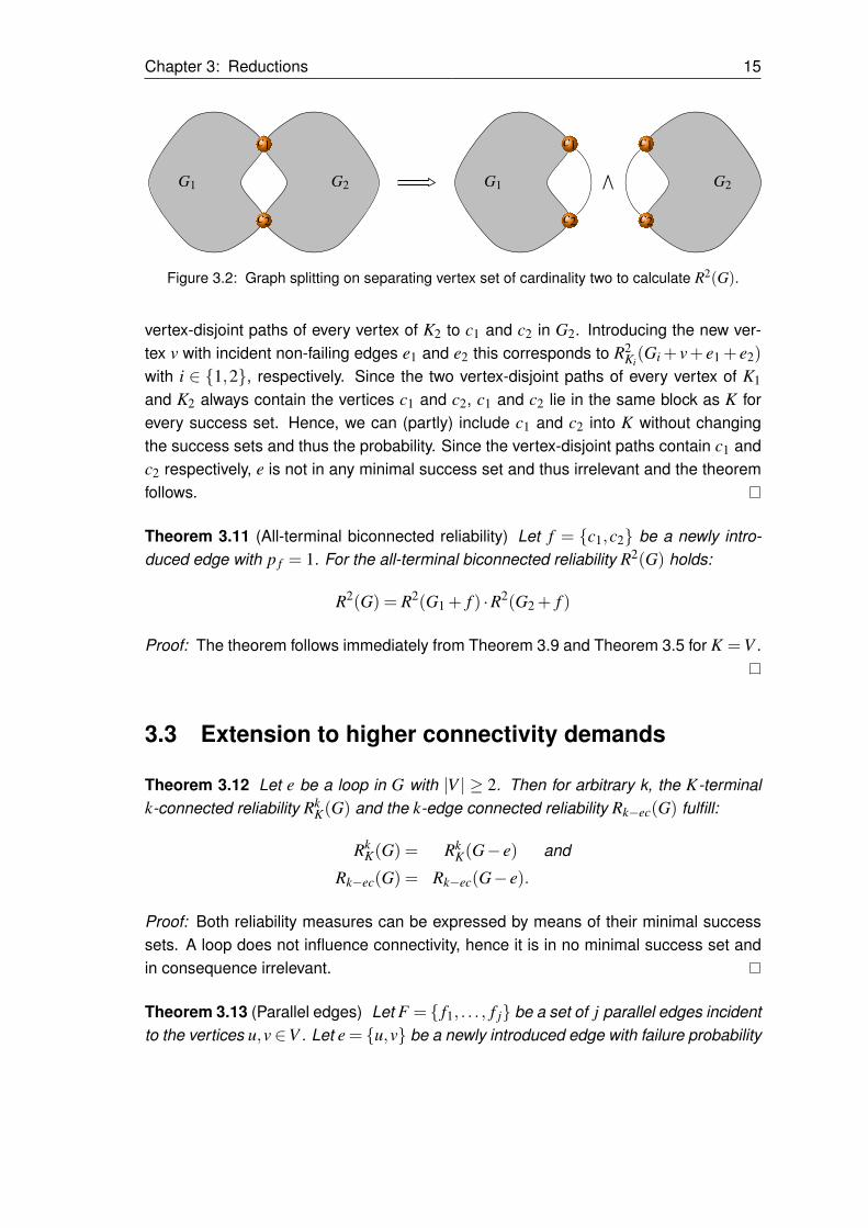
3.2 Graph splitting on separating vertex set of cardinality two to calculate R2(G). . . . . . . . . . . . 15
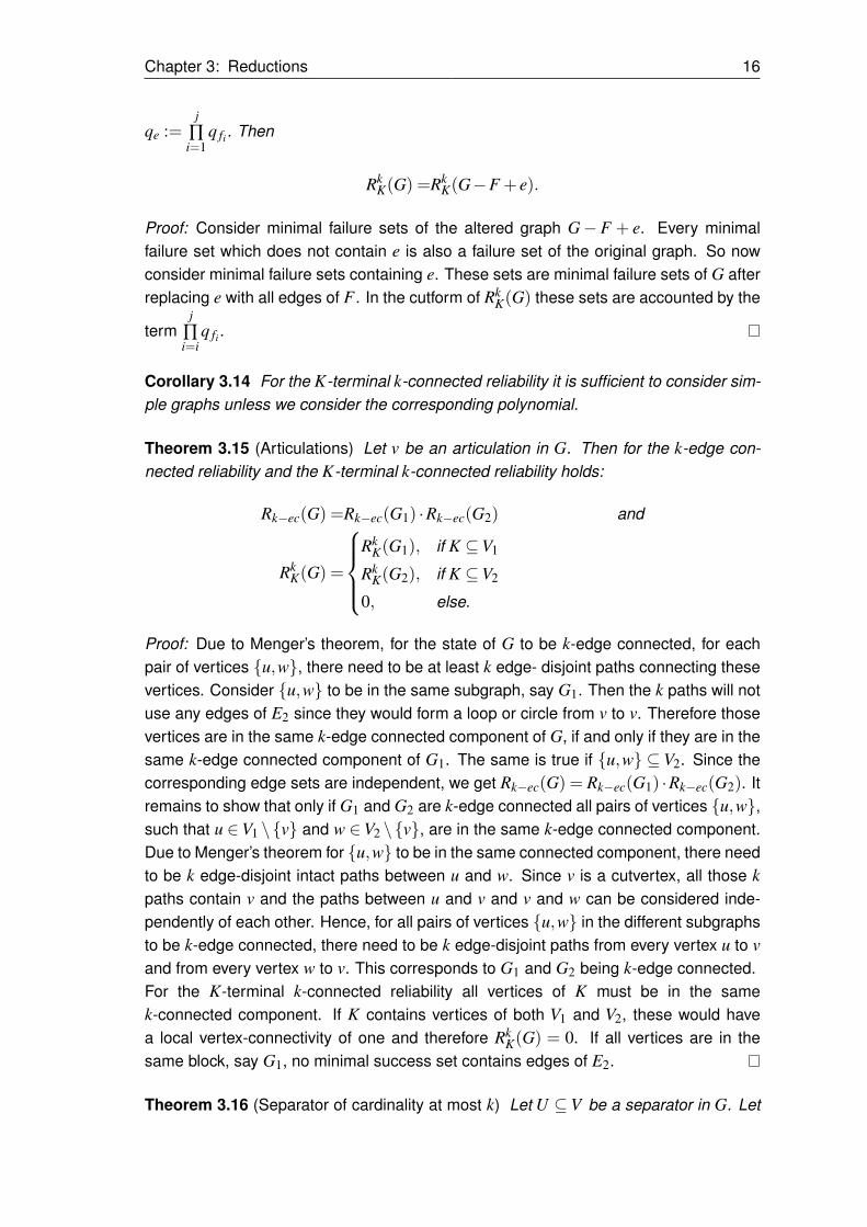
3.3 Failure state corresponding to a success state after splitting for |U |= 3 > k = 2. . . . . . . . 18
4.1 Partitioning of V (G) depending on connectivity to fixed vertex v . . . . . . . . . . . . . . . . . . . . . . . . . . 23
4.2 The vertex set S: All edges incident to v are bridges. . . . . . . . . . . . . . . . . . . . . . . . . . . . . . . . . . . . . . . 24
4.3 Decomposition of Gk,l into connected components after edge failure . . . . . . . . . . . . . . . . . . . . . 25
4.4 The vertex set T : Vertices having a common block with v . . . . . . . . . . . . . . . . . . . . . . . . . . . . . . . . . 27
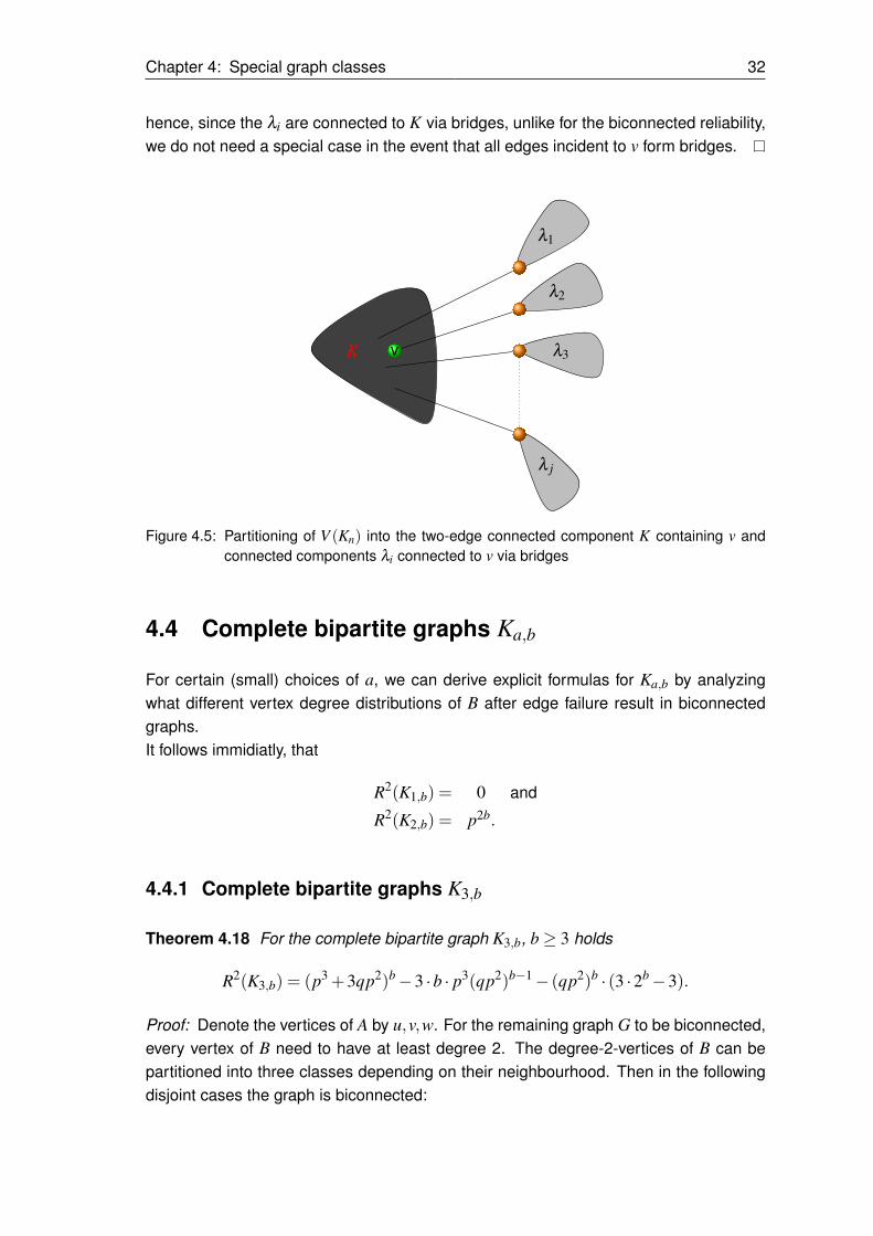
4.5 Partitioning of V (Kn) into the two-edge connected component K containing v and con-
nected components λi connected to v via bridges . . . . . . . . . . . . . . . . . . . . . . . . . . . . . . . . . . . . . . . . . 32
4.6 Vertex partitioning used to calculate R2(Ka,b) . . . . . . . . . . . . . . . . . . . . . . . . . . . . . . . . . . . . . . . . . . . . . . 37
4.7 Partitioning of the vertex set S . . . . . . . . . . . . . . . . . . . . . . . . . . . . . . . . . . . . . . . . . . . . . . . . . . . . . . . . . . . . . . . 37
4.8 Vertex partitioning used to calculate R2−ec(Ka,b) . . . . . . . . . . . . . . . . . . . . . . . . . . . . . . . . . . . . . . . . . . . 43
5.1 Structure of G in Theorem 5.3. . . . . . . . . . . . . . . . . . . . . . . . . . . . . . . . . . . . . . . . . . . . . . . . . . . . . . . . . . . . . . . 44
5.2 Graph with irrelevant edges which do not join separators of cardinality two . . . . . . . . . . . . . . 46

III
III. List of Tables
4.1 Number of biconnected graphs on n vertices. . . . . . . . . . . . . . . . . . . . . . . . . . . . . . . . . . . . . . . . . . . . . . . 28
4.2 Runtime and space requirement of the subfunctions used to calculate R2(Kn) . . . . . . . . . . 30
IV
IV. Preface
Computer communication networks play a mayor role to manage data transfer and in-formation processing. However, the components of the network may fail - by targetedattacks or by wearout. While targeted attacks are non-random, it seems appropriate toconsider wearout effects as random. Further we can assume that the components failindependently. The task of network reliability is to analyze networks in respect to thefunctionality of the network with consideration of wearout of its components. In mostcases a network is considered as functional if a selected set of terminals can commu-nicate. However, in practical applications additional restrictions to data capacities ofthe components or limited time delay in the communication apply. We will consider thespecial case were all connections have unit capacity while we want to transfer two datapackages between selected vertices. Alternatively, one could consider the so-called bi-connected reliability as the probability that the network can communicate under wearouteven after a targeted attack destructed one vertex.
Chapter 1: Preliminaries 1
1 Preliminaries
1.1 Graph notations
We presume that the reader is familiar with the basics of graph theory. Therefore we willonly give the used notation for common graph concepts.
In general by V we will denote the vertex set of the graph G and by E the edge set of G.NG(v) of a vertex v ∈ V is the set of vertices adjacent to v in G and is called openneighbourhood of v.NG[v] := NG(v)∪{v} denotes the closed neighbourhood of v.For vertex subsets W ⊆V , we define the open and closed neighbourhood by
NG(W ) :=⋃
v∈W
NG(v)\W and NG[W ] :=NG(W )∪W.
δW denotes the set of edges between W and V \W .δ denotes the minimum degree of G and ∆ is the maximum degree of G.A separator is a vertex subset S⊆V such that there exist two graphs G1 = (V1,E1) andG2 = (V2,E2) with G = G1∪G2, V1∩V2 = S. An articulation is a separator of cardinalityone.A cutset is an edge subset C ⊆ E, such that there exist two graphs G1 = (V1,E1) andG2 = (V2,E2) with G−C = G1∪G2 and V1∩V2 = /0.
1.2 Graph operations
For a graph G = (V,E) we use the following graph operations:
G− e := (V,E \{e}) is the graph resulting from G after deletion of the edge e.G− v := (V \{v},E \δ{v}) is the resulting graph from G after deletion of the vertex v
and all edges incident to v.G−F := (V,E \F) is the graph resulting from G after deleting all edges of F .G−W := (V \W,{{x,y} ∈ E|x,y ∈V \W}) is the graph resulting from G after deletion
of all vertices of W ⊆V and all edges incident to vertices of W .G+ e := (V,E∪{e}) is the graph resulting from G after insertion of the edge e (resulting
multiple edges will be conserved).G+ v := (V ∪{v},E) is the graph after insertion of a new vertex v.G<W> := (W,{x,y} ∈ E|x,y ∈W ) is the induced subgraph of G.G(F) := (V,F) = G− (E \F).
Chapter 1: Preliminaries 2
G/e is the resulting graph of G after contraction of the edge e ∈ E (identifying the endvertices of e and conserving multiple edges).
G+H := (V (H)∪V (G),E(H)∪E(G)∪{{u,v}|u ∈V (H),v ∈V (G)}) is the join of thegraphs G and H. We will assume that V (H)∩V (G) = /0.
For a probabilistic graph (see Definition 2.1), we have all those graph operations, whileleaving the edge probabilities unchanged (for G+e and G+H the probability of the newedge(s) will be given explicitly). Additionally, we have the operation G|pe=k, which willleave the graph unchanged while changing the edge probability of e to the value k.
1.3 Graph connectivity
Since the focus of this thesis is the reliability of two-connected graphs, we will defineconnectivity in detail and characterize two-connected graphs.The local vertex-connectivity function κ(x,y), defined for every pair of non-adjacent ver-tices, is the minimum number of vertices, whose omission from G disconnects x andy. The local edge-connectivity function λ (x,y), defined for every pair of vertices, is theminimum number of edges, whose omission from G disconnects x and y. The vertex-connectivity κ(G) = minκ(x,y) is the global minimum of the local vertex-connectivity.Similarly, the edge-connectivity λ (G) = minλ (x,y) is the global minimum of the localedge-connectivity. For the complete graph of order n, Kn, we define the connectivity as:κ(Kn) = λ (Kn) = n−1. A graph G is called k-connected if and only if κ(G)≥ k and iscalled k-edge-connected if and only if λ (G)≥ k.In this thesis we will use the terms two-connected, biconnected and non-separable assynonyms and therefore explicitly exclude the K2 from the latter. A block of a graph is abiconnected component of a graph.A vertex set V1 is connected to a vertex v via a vertex set V2 in G if and only if thefollowing holds:
• V1,V2 and v are in the same connected component of G• In the graph G−V2 for all u ∈V1 holds: u and v are not connected.
The most important result linking connectivity to pathsets is due to Menger’s famoustheorem [Men27] which we will now state as presented by Bollobás [Bol04].
Theorem 1.1 (Menger’s Theorem) A graph G is k-connected (resp. k-edge-connected)if and only if for any two vertices there are k disjoint (resp. k edge-disjoint) paths joiningthem.
Proof: For the proof see [Men27]. Other elegant proofs dued to Dirac and Pym can befound in [Dir66] and [Pym69].
Chapter 1: Preliminaries 3
Therefore we call two vertices u,v biconnected if and only if there exist two disjoint pathsbetween u and v, that means u and v are in a common block.
Two-connected graphs can be characterized by the following theorem:
Theorem 1.2 Let G be a graph with |V | ≥ 3. Then the following conditions are equiva-lent.
• G is two-connected.• G has no articulation.• Given any two vertices there is a cycle containing them.• Given any vertex and any edge there is a cycle containing them.• Given any two edges there is a cycle containing them.
Proof: The proof can be found in [Plu68].
1.4 Special graph classes
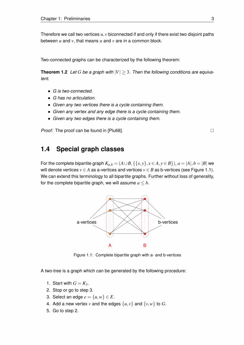
For the complete bipartite graph Ka,b = (A∪B,{{x,y},x∈ A,y∈ B}), a = |A|,b = |B| wewill denote vertices v∈ A as a-vertices and vertices v∈ B as b-vertices (see Figure 1.1).We can extend this terminology to all bipartite graphs. Further without loss of generality,for the complete bipartite graph, we will assume a≤ b.
a-vertices b-vertices
BA
Figure 1.1: Complete bipartite graph with a- and b-vertices
A two-tree is a graph which can be generated by the following procedure:
1. Start with G = K3.2. Stop or go to step 3.3. Select an edge e = {u,w} ∈ E.4. Add a new vertex v and the edges {u,v} and {v,w} to G.5. Go to step 2.
Chapter 1: Preliminaries 4
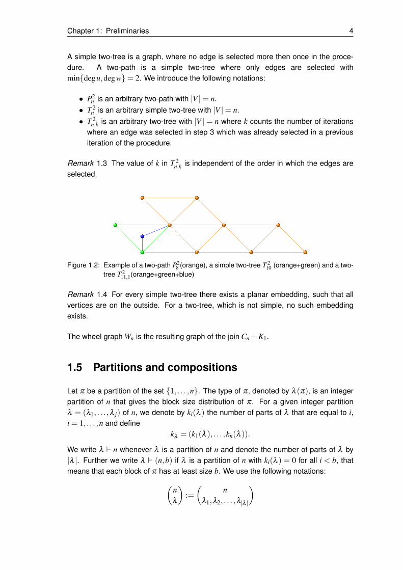
A simple two-tree is a graph, where no edge is selected more then once in the proce-dure. A two-path is a simple two-tree where only edges are selected withmin{degu,degw}= 2. We introduce the following notations:
• P2n is an arbitrary two-path with |V |= n.
• T 2n is an arbitrary simple two-tree with |V |= n.
• T 2n,k is an arbitrary two-tree with |V | = n where k counts the number of iterations
where an edge was selected in step 3 which was already selected in a previousiteration of the procedure.
Remark 1.3 The value of k in T 2n,k is independent of the order in which the edges are
selected.
Figure 1.2: Example of a two-path P28 (orange), a simple two-tree T 2
10 (orange+green) and a two-tree T 2
11,1(orange+green+blue)
Remark 1.4 For every simple two-tree there exists a planar embedding, such that allvertices are on the outside. For a two-tree, which is not simple, no such embeddingexists.
The wheel graph Wn is the resulting graph of the join Cn +K1.
1.5 Partitions and compositions
Let π be a partition of the set {1, . . . ,n}. The type of π , denoted by λ (π), is an integerpartition of n that gives the block size distribution of π . For a given integer partitionλ = (λ1, . . . ,λ j) of n, we denote by ki(λ ) the number of parts of λ that are equal to i,i = 1, . . . ,n and define
kλ = (k1(λ ), . . . ,kn(λ )).
We write λ ` n whenever λ is a partition of n and denote the number of parts of λ by|λ |. Further we write λ ` (n,b) if λ is a partition of n with ki(λ ) = 0 for all i < b, thatmeans that each block of π has at least size b. We use the following notations:(
nλ
):=(
nλ1,λ2, . . . ,λ|λ |
)

Chapter 1: Preliminaries 5
kλ ! :=n
∏i=1
ki(λ )!{nλ
}:=
1kλ !
(nλ
)where the last expression equals the number of set partitions of {1, . . . ,n} of the giventype λ ` n.We write λ � n if λ = (λ1, . . . ,λr) is a composition (ordered integer partition) of n. Weintroduce the following additional notations:
• λ � (n,s) :⇔ λ � n and |λ |= s
• λ � (n,s,b) :⇔ n =s∑
i=1λi and λi ≥ b for all i
•(
nλ
):=(
nλ1, . . . ,λ|λ |
)Remark 1.5 It can easily be verified, that λ � (n,s,b)⇔ λ − (b−1) � (n− (b−1) · s,s)where λ − (b− 1) means that each part of λ is reduced by b− 1. Therefore the set{λ : λ � (n,s,b)} for given n, s and b is finite even for b≤ 0.
Chapter 2: Reliability measures 6
2 Reliability measures
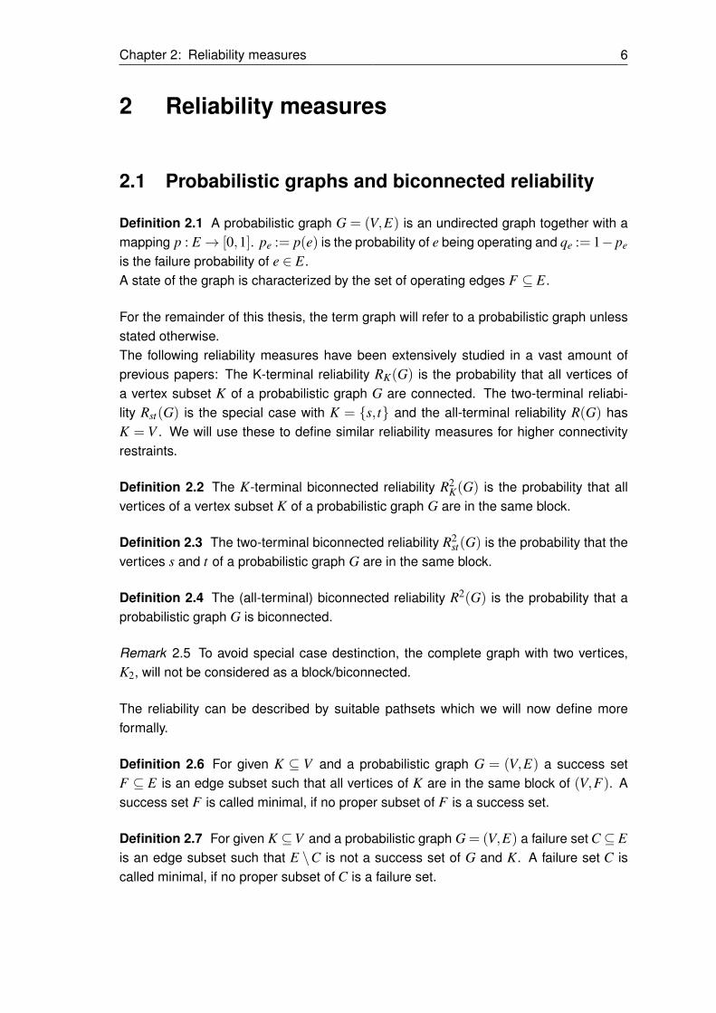
2.1 Probabilistic graphs and biconnected reliability
Definition 2.1 A probabilistic graph G = (V,E) is an undirected graph together with amapping p : E→ [0,1]. pe := p(e) is the probability of e being operating and qe := 1− pe
is the failure probability of e ∈ E.A state of the graph is characterized by the set of operating edges F ⊆ E.
For the remainder of this thesis, the term graph will refer to a probabilistic graph unlessstated otherwise.The following reliability measures have been extensively studied in a vast amount ofprevious papers: The K-terminal reliability RK(G) is the probability that all vertices ofa vertex subset K of a probabilistic graph G are connected. The two-terminal reliabi-lity Rst(G) is the special case with K = {s, t} and the all-terminal reliability R(G) hasK = V . We will use these to define similar reliability measures for higher connectivityrestraints.
Definition 2.2 The K-terminal biconnected reliability R2K(G) is the probability that all
vertices of a vertex subset K of a probabilistic graph G are in the same block.
Definition 2.3 The two-terminal biconnected reliability R2st(G) is the probability that the
vertices s and t of a probabilistic graph G are in the same block.
Definition 2.4 The (all-terminal) biconnected reliability R2(G) is the probability that aprobabilistic graph G is biconnected.
Remark 2.5 To avoid special case destinction, the complete graph with two vertices,K2, will not be considered as a block/biconnected.
The reliability can be described by suitable pathsets which we will now define moreformally.
Definition 2.6 For given K ⊆ V and a probabilistic graph G = (V,E) a success setF ⊆ E is an edge subset such that all vertices of K are in the same block of (V,F). Asuccess set F is called minimal, if no proper subset of F is a success set.
Definition 2.7 For given K ⊆V and a probabilistic graph G = (V,E) a failure set C⊆ Eis an edge subset such that E \C is not a success set of G and K. A failure set C iscalled minimal, if no proper subset of C is a failure set.
Chapter 2: Reliability measures 7
With F and C we will denote the set of success sets and failure sets of G and K. F ′
and C ′ will denote the corresponding sets of minimal success and failure sets.
Definition 2.8 Let G be a two-connected graph.An edge e is essential, if and only if e is part of every minimal success set.An edge e is irrelevant, if and only if e is part of no minimal success set.
Since success and failure sets correspond to states of the probabilistic graph and edgesfail independently, we can calculate the K-terminal-biconnected reliability of G, wherewe compound the edge probabilities in the vector p, by the following formulas:
R2K(G,p) = ∑
F∈F∏e∈F
pe ∏f∈E\F
(1− p f ) (2.1)
=1− ∑C∈C
∏e∈C
(1− pe) ∏f∈E\C
p f (2.2)
where from now on for simplicity we will omit p and simply write R2K(G).
Remark 2.9 Since every superset of a minimal success/failure set is a success/failureset as well, F and C are completly described by F ′ and C ′. Therefore, the biconnected-reliability can be calculated via the minimal success and failure sets, even though anexplicit formula will not be given here.
Remark 2.10 Let G be a biconnected graph. If e is an essential edge, G− e is notbiconnected and hence it holds R2
K(G− e) = 0. If e is an irrelevant edge, it holdsR2
K(G) = R2K(G− e). Further, G− e has the same minimal success and failure sets
as G. Hence, the removal of an irrelevant edge e does not change the characterisationof other edges as essential and irrelevant edges.
If all edges fail with the same probability p, the biconnected reliability becomes a poly-nomial in p or q = 1− p:
R2K(G, p) = ∑
F∈Fp|F |(1− p)|E|−|F | (2.3)
=1− ∑C∈C
(1− p)|C|p|E|−|C| (2.4)
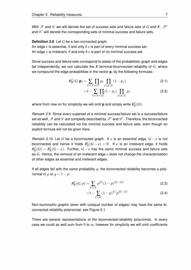
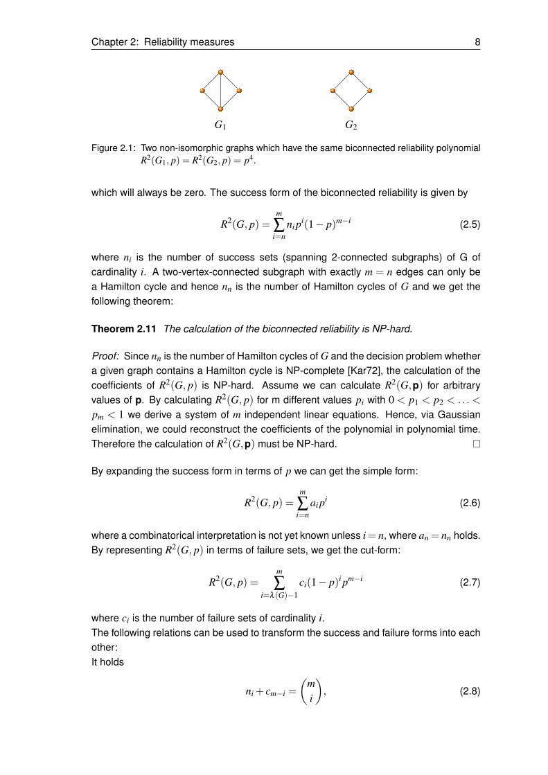
Non-isomorphic graphs (even with unequal number of edges) may have the same bi-connected reliability polynomial, see Figure 2.1.
There are several representations of the biconnected-reliability polynomial. In everycase we could as well sum from 0 to m, however for simplicity we will omit coefficients
Chapter 2: Reliability measures 8
G1 G2
Figure 2.1: Two non-isomorphic graphs which have the same biconnected reliability polynomialR2(G1, p) = R2(G2, p) = p4.
which will always be zero. The success form of the biconnected reliability is given by
R2(G, p) =m
∑i=n
ni pi(1− p)m−i (2.5)
where ni is the number of success sets (spanning 2-connected subgraphs) of G ofcardinality i. A two-vertex-connected subgraph with exactly m = n edges can only bea Hamilton cycle and hence nn is the number of Hamilton cycles of G and we get thefollowing theorem:
Theorem 2.11 The calculation of the biconnected reliability is NP-hard.
Proof: Since nn is the number of Hamilton cycles of G and the decision problem whethera given graph contains a Hamilton cycle is NP-complete [Kar72], the calculation of thecoefficients of R2(G, p) is NP-hard. Assume we can calculate R2(G,p) for arbitraryvalues of p. By calculating R2(G, p) for m different values pi with 0 < p1 < p2 < .. . <
pm < 1 we derive a system of m independent linear equations. Hence, via Gaussianelimination, we could reconstruct the coefficients of the polynomial in polynomial time.Therefore the calculation of R2(G,p) must be NP-hard.
By expanding the success form in terms of p we can get the simple form:
R2(G, p) =m
∑i=n
ai pi (2.6)
where a combinatorical interpretation is not yet known unless i= n, where an = nn holds.By representing R2(G, p) in terms of failure sets, we get the cut-form:
R2(G, p) =m
∑i=λ (G)−1
ci(1− p)i pm−i (2.7)
where ci is the number of failure sets of cardinality i.The following relations can be used to transform the success and failure forms into eachother:It holds
ni + cm−i =
(mi
), (2.8)
Chapter 2: Reliability measures 9
since for every edge subset F ⊆ E, |F | = i one of the following things can happen: Fis a success set (counted by ni) or it is not, in which case E \F must be a failure set(counted by cm−i).The simple form is linked to the success form via the following relation:
nl =l−1
∑i=0
(m− l + i
i
)al−i (2.9)
which follows immediately from the expansion of the success form to derive the simpleform. Further representations of the reliability polynomial which can be transferred tothe biconnected reliability can be found for example in [Col91].Since we can calculate the biconnected reliability via pathsets, we get the followingformula:
Theorem 2.12 Let G be a probabilistic graph. Then for every edge e ∈ E and everyK ⊆V holds:
R2K(G) = (1− pe) ·R2
K(G− e)+ pe ·R2K(G|pe=1)
Proof: The K-terminal biconnected reliability can be expressed via pathsets:
R2K(G) = ∑
F∈F (G)∏f∈F
p f ∏g∈E\F
(1− pg)
= ∑F∈F (G),e∈F
∏f∈F
p f ∏g∈E\F
(1− pg)+ ∑F∈F (G),e6∈F
∏f∈F
p f ∏g∈E\F
(1− pg)
=pe · ∑F∈F (G),e∈F
∏f∈F, f 6=e
p f ∏g∈E\F
(1− pg)
+(1− pe) · ∑F∈F (G),e6∈F
∏f∈F
p f ∏g∈E\F,g6=e
(1− pg)
=pe · ∑F∈F (G|pe=1),e∈F
∏f∈F
p f ∏g∈E\F
(1− pg)
+(1− pe) · ∑F∈F (G−e)
∏f∈F
p f ∏g∈(E−{e})\F
(1− pg)
=pe ·R2K(G|pe=1)+(1− pe) ·R2
K(G− e)
Remark 2.13 Unlike for the all-terminal reliability, in general it does not hold
R2K(G|pe=1) = R2
K(G/e),
see for example Figure 2.2.
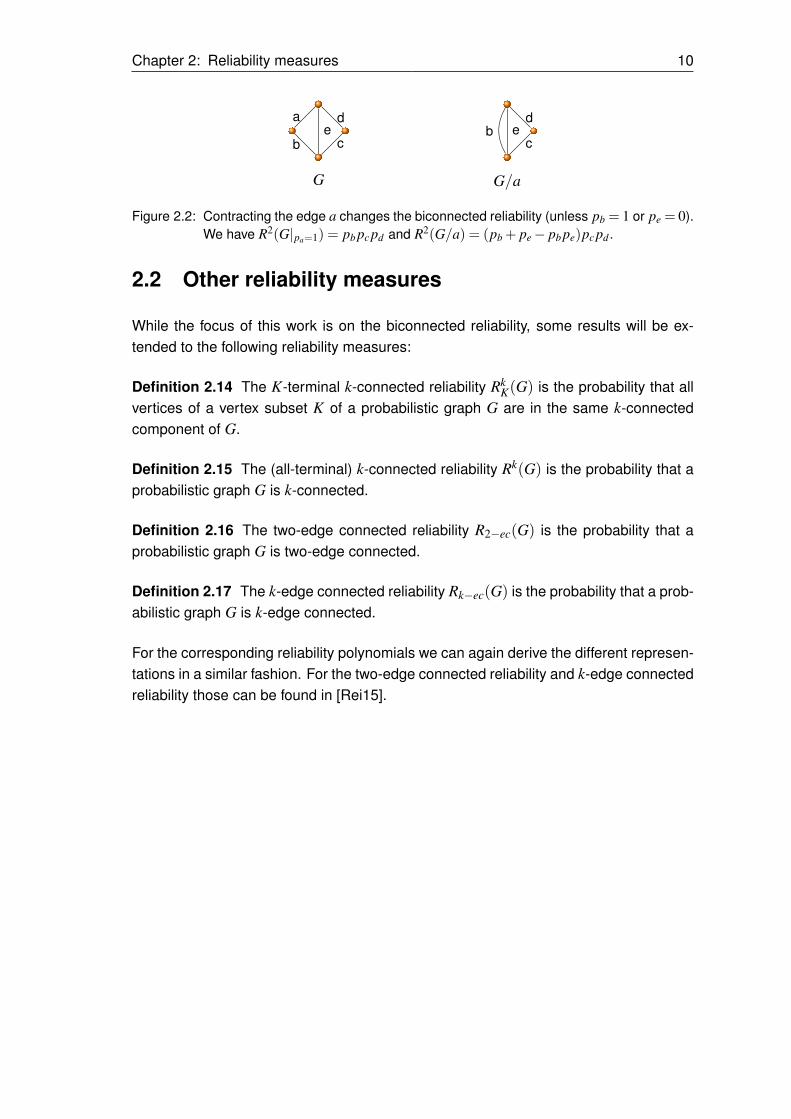
Chapter 2: Reliability measures 10
a
b c
de
G
bc
de
G/a
Figure 2.2: Contracting the edge a changes the biconnected reliability (unless pb = 1 or pe = 0).We have R2(G|pa=1) = pb pc pd and R2(G/a) = (pb + pe− pb pe)pc pd .
2.2 Other reliability measures
While the focus of this work is on the biconnected reliability, some results will be ex-tended to the following reliability measures:
Definition 2.14 The K-terminal k-connected reliability RkK(G) is the probability that all
vertices of a vertex subset K of a probabilistic graph G are in the same k-connectedcomponent of G.
Definition 2.15 The (all-terminal) k-connected reliability Rk(G) is the probability that aprobabilistic graph G is k-connected.
Definition 2.16 The two-edge connected reliability R2−ec(G) is the probability that aprobabilistic graph G is two-edge connected.
Definition 2.17 The k-edge connected reliability Rk−ec(G) is the probability that a prob-abilistic graph G is k-edge connected.
For the corresponding reliability polynomials we can again derive the different represen-tations in a similar fashion. For the two-edge connected reliability and k-edge connectedreliability those can be found in [Rei15].
Chapter 3: Reductions 11
3 Reductions
3.1 Series-Parallel reductions and articulations
Theorem 3.1 Let e ∈ E be a loop of G. Then for all K ⊆V it holds:
R2K(G) = R2
K(G− e).
Proof: The K-terminal biconnected reliability can be calculated via the set of all inclusion-minimal success sets. Assume e is part of a minimal success set F , that means that allvertices of K are within the same block in (G,F) but not in (G,F − e). But since e is aloop, (G,F) and (G,F− e) have exactly the same blocks, therefore e can not be a partof a minimal success set and the theorem holds.
Theorem 3.2 (Parallel reduction) Let F := { f1, . . . , fk} be a set of k ≥ 2 parallel edgesincident to the vertices u and v with the corresponding probabilities of failure q1, . . .qk.Let e = {u,v} be a newly introduced edge between u and v with failure probabilityqe = ∏
ki=1 qi.
Then for all K ⊆V,K 6= {u,v}, the following statement holds:
R2K(G) = R2
K(G−F + e).
For K = {u,v} it holds:
R2uv(G) = 1+(R2
uv(G−F)−1) ·k
∏i=1
qi +(Ruv(G−F)−1) ·k
∏i=1
qi · ∑f∈F
p f
q f.
Proof: Every minimal failure set of the altered graph which does not use e is exactly aminimal failure set in the original graph. So now consider minimal failure sets of the newgraph which use e. In the original graph those sets without e form a failure set with alledges of e1, . . . ,ek. On the other hand, no minimal failure set uses e1, . . . ,ek partly, andtherefore the minimal failure sets of the original graph and the altered graph have anone-to-one correspondence with the given new probability to account for the failure ofall edges e1, . . . ,ek.The result for K = {u,v} follows immediately from Theorem 2.12.
Corollary 3.3 For the biconnected reliability it is sufficient to consider simple graphsunless we consider the biconnected reliability polynomial.
Theorem 3.4 (Articulations) Let G = (V,E) be a graph and v ∈ V an articulation of G.
Chapter 3: Reductions 12
Then for all K ⊆V holds:
R2K(G) =
R2
K(G1), if K ⊆V1
R2K(G2), if K ⊆V2
0, otherwise.
Proof: If K 6⊆ V1 and K 6⊆ V2, then K contains vertices v1,v2 such that v1 ∈ V1 \ {v},v2 ∈ V2 \ {v}. Since v is an articulation in G, all paths between v1 and v2 have v incommon, therefore the biconnected reliability is 0. Without loss of generality now letK ⊆ V1. Then no inclusion-minimal success set of G contains edges of E2 since theseedges would form a loop or circle from v to v. Hence, all edges of E2 are irrelevant andwe get R2
K(G) = R2K(G−E2) = R2
K(G1) (isolated vertices in V \K can be omitted).
Theorem 3.5 (Series-Reduction) Let v ∈ V be a vertex of G with degv = 2. Lete1, e2 ∈ E be the edges incident to v with the corresponding probabilities p1 and p2.Furthermore, let u,w ∈ NG(v) be the vertices adjacent to v and e := {u,w} be a newedge incident to u and w. Then the following holds:
• If v 6∈ K: R2K(G) = R2
K(G− v+ e) with pe = p1 p2
• If v ∈ K:
R2K(G) = p1 p2 ·R2
K(G|p1=p2=1)
= p1 p2 ·R2K∪{u,w}(G− v+ e|pe=1).
Proof: First, let v 6∈ K. If a minimal success set in G− v+ e does not contain e, it is aminimal success set in G as well. Further, there exists a one-to-one corresponding ofminimal success sets of G−v+e containing e and minimal success sets of G containinge1 and e2 instead.Now, let v ∈ K. If e1 or e2 fail, then v is no longer in a block with the other vertices of v.Therefore, by Theorem 2.12 the first equality holds. For K to be in the same block in Gthere must be vertex-disjoint paths from every vertex of K to u and w. If we introduce thenew edge e between u and w, then K, u and w are in the same block in G− v+ e.
Corollary 3.6 The biconnected reliability of series-parallel graphs can be calculated inlinear time.
3.2 Reductions on separators of cardinality two
Let {c1,c2} be a separator of cardinality two of G = (V,E). Let e ∈ E1∩E2, if existing,denote the edge between the two cut-vertices.
Theorem 3.7 (Two-terminal biconnected reliability) Let v be a new vertex ande1 = {c1,v}, e2 = {c2,v} two edges incident to v and the cut vertices with pe1 = pe2 = 1.
Chapter 3: Reductions 13
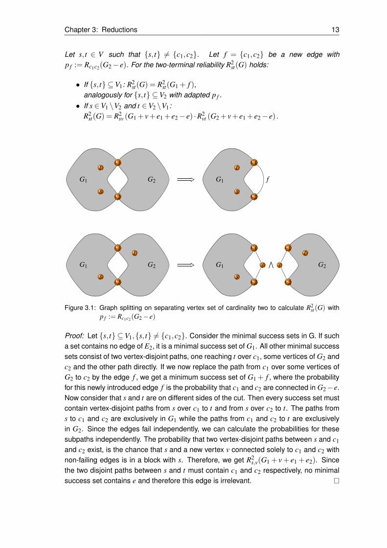
Let s, t ∈ V such that {s, t} 6= {c1,c2}. Let f = {c1,c2} be a new edge withp f := Rc1c2(G2− e). For the two-terminal reliability R2
st(G) holds:
• If {s, t} ⊆V1: R2st(G) = R2
st(G1 + f ),analogously for {s, t} ⊆V2 with adapted p f .• If s ∈V1 \V2 and t ∈V2 \V1:
R2st(G) = R2
sv (G1 + v+ e1 + e2− e) ·R2vt (G2 + v+ e1 + e2− e) .
G2G1
s
tc1
c2
G1
s
tc1
c2
f
G2
t
G1
s
c1
c2
G1
s
c1
c2
v G2
tc1
c2
v∧
Figure 3.1: Graph splitting on separating vertex set of cardinality two to calculate R2st(G) with
p f := Rc1c2(G2− e)
Proof: Let {s, t} ⊆V1,{s, t} 6= {c1,c2}. Consider the minimal success sets in G. If sucha set contains no edge of E2, it is a minimal success set of G1. All other minimal successsets consist of two vertex-disjoint paths, one reaching t over c1, some vertices of G2 andc2 and the other path directly. If we now replace the path from c1 over some vertices ofG2 to c2 by the edge f , we get a minimum success set of G1 + f , where the probabilityfor this newly introduced edge f is the probability that c1 and c2 are connected in G2−e.Now consider that s and t are on different sides of the cut. Then every success set mustcontain vertex-disjoint paths from s over c1 to t and from s over c2 to t. The paths froms to c1 and c2 are exclusively in G1 while the paths from c1 and c2 to t are exclusivelyin G2. Since the edges fail independently, we can calculate the probabilities for thesesubpaths independently. The probability that two vertex-disjoint paths between s and c1
and c2 exist, is the chance that s and a new vertex v connected solely to c1 and c2 withnon-failing edges is in a block with s. Therefore, we get R2
s,v(G1 + v+ e1 + e2). Sincethe two disjoint paths between s and t must contain c1 and c2 respectively, no minimalsuccess set contains e and therefore this edge is irrelevant.
Chapter 3: Reductions 14
Theorem 3.8 (Two-terminal biconnected reliability) Let {s, t}= {c1,c2} and {s, t} 6∈ E.Then
R2st(G) =R2
st(G1)+R2st(G2)−R2
st(G1) ·R2st(G2)
+(Rst(G1)−R2
st(G1))·(Rst(G2)−R2
st(G2)).
Proof: The following events result in s and t being biconnected:
• There exist two vertex-disjoint paths between s and t in G1.• There exist two vertex-disjoint paths between s and t in G2.• G1 and G2 each contain one path from s to t.
The probability for exactly one path in G1 can be described as(Rst(G1)−R2
st(G1)).
The theorem follows by inclusion-exclusion.
Theorem 3.9 (K-terminal biconnected reliability) Let f = {c1,c2} be a new edge withp f = Rc1c2(G2− e) and v a new vertex as in Theorem 3.7. For all K ⊆ V with |K| ≥ 3holds:
• If K ⊆V1: R2K(G) = R2
K(G1 + f ).Analogously for K ⊆V2 with adapted p f .• If K 6⊆V1 and K 6⊆V2:
R2K(G) =R2
K∪{c1,c2}(G− e)
=R2K′1(G1 + v+ e1 + e2− e) ·R2
K′2(G2 + v+ e1 + e2− e)
with (K∩Vi)∪{v} ⊆ K′i ⊆ (K∩Vi)∪{v,c1,c2}, i ∈ {1,2}
Remark 3.10 The second case of the theorem allows us to arbitrarily select/deselectthe vertices c1 and c2 for the terminal set K which in some cases may allow us to reachthe special cases of two-terminal or all-terminal biconnected-reliability.
Proof: First, consider the case that K ⊆ V1. For every minimal success set of G thefollowing holds: Either the success sets contains no edge of E2 \ {e} or it containsexactly one path connecting c1 and c2 in G2 − e. The former corresponds tominimal success sets of G1, the latter corresponds to minimal success sets of G1 + fcontaining f .Now consider the case that K contains vertices of both V1 and V2. Let K1 := K \V2 6= /0and let K2 =K\V1 6= /0. For all vertices of K to build a block in the remaining graph, everysuccess set must contain two vertex-disjoint paths between every vertex of K1 and K2
which corresponds to vertex-disjoint paths of every vertex of K1 to c1 and c2 in G1 and
Chapter 3: Reductions 15
G2G1
c1
c2
G1
c1
c2
G2
c1
c2
∧
Figure 3.2: Graph splitting on separating vertex set of cardinality two to calculate R2(G).
vertex-disjoint paths of every vertex of K2 to c1 and c2 in G2. Introducing the new ver-tex v with incident non-failing edges e1 and e2 this corresponds to R2
Ki(Gi + v+ e1 + e2)
with i ∈ {1,2}, respectively. Since the two vertex-disjoint paths of every vertex of K1
and K2 always contain the vertices c1 and c2, c1 and c2 lie in the same block as K forevery success set. Hence, we can (partly) include c1 and c2 into K without changingthe success sets and thus the probability. Since the vertex-disjoint paths contain c1 andc2 respectively, e is not in any minimal success set and thus irrelevant and the theoremfollows.
Theorem 3.11 (All-terminal biconnected reliability) Let f = {c1,c2} be a newly intro-duced edge with p f = 1. For the all-terminal biconnected reliability R2(G) holds:
R2(G) = R2(G1 + f ) ·R2(G2 + f )
Proof: The theorem follows immediately from Theorem 3.9 and Theorem 3.5 for K =V .
3.3 Extension to higher connectivity demands
Theorem 3.12 Let e be a loop in G with |V | ≥ 2. Then for arbitrary k, the K-terminalk-connected reliability Rk
K(G) and the k-edge connected reliability Rk−ec(G) fulfill:
RkK(G) = Rk
K(G− e) and
Rk−ec(G) = Rk−ec(G− e).
Proof: Both reliability measures can be expressed by means of their minimal successsets. A loop does not influence connectivity, hence it is in no minimal success set andin consequence irrelevant.
Theorem 3.13 (Parallel edges) Let F = { f1, . . . , f j} be a set of j parallel edges incidentto the vertices u,v∈V . Let e = {u,v} be a newly introduced edge with failure probability
Chapter 3: Reductions 16
qe :=j
∏i=1
q fi . Then
RkK(G) =Rk
K(G−F + e).
Proof: Consider minimal failure sets of the altered graph G− F + e. Every minimalfailure set which does not contain e is also a failure set of the original graph. So nowconsider minimal failure sets containing e. These sets are minimal failure sets of G afterreplacing e with all edges of F . In the cutform of Rk
K(G) these sets are accounted by the
termj
∏i=i
q fi .
Corollary 3.14 For the K-terminal k-connected reliability it is sufficient to consider sim-ple graphs unless we consider the corresponding polynomial.
Theorem 3.15 (Articulations) Let v be an articulation in G. Then for the k-edge con-nected reliability and the K-terminal k-connected reliability holds:
Rk−ec(G) =Rk−ec(G1) ·Rk−ec(G2) and
RkK(G) =
Rk
K(G1), if K ⊆V1
RkK(G2), if K ⊆V2
0, else.
Proof: Due to Menger’s theorem, for the state of G to be k-edge connected, for eachpair of vertices {u,w}, there need to be at least k edge- disjoint paths connecting thesevertices. Consider {u,w} to be in the same subgraph, say G1. Then the k paths will notuse any edges of E2 since they would form a loop or circle from v to v. Therefore thosevertices are in the same k-edge connected component of G, if and only if they are in thesame k-edge connected component of G1. The same is true if {u,w} ⊆ V2. Since thecorresponding edge sets are independent, we get Rk−ec(G) = Rk−ec(G1) ·Rk−ec(G2). Itremains to show that only if G1 and G2 are k-edge connected all pairs of vertices {u,w},such that u ∈V1 \{v} and w ∈V2 \{v}, are in the same k-edge connected component.Due to Menger’s theorem for {u,w} to be in the same connected component, there needto be k edge-disjoint intact paths between u and w. Since v is a cutvertex, all those kpaths contain v and the paths between u and v and v and w can be considered inde-pendently of each other. Hence, for all pairs of vertices {u,w} in the different subgraphsto be k-edge connected, there need to be k edge-disjoint paths from every vertex u to vand from every vertex w to v. This corresponds to G1 and G2 being k-edge connected.For the K-terminal k-connected reliability all vertices of K must be in the samek-connected component. If K contains vertices of both V1 and V2, these would havea local vertex-connectivity of one and therefore Rk
K(G) = 0. If all vertices are in thesame block, say G1, no minimal success set contains edges of E2.
Theorem 3.16 (Separator of cardinality at most k) Let U ⊆V be a separator in G. Let
Chapter 3: Reductions 17
K1 := K ∩V1 \U 6= /0 and K2 := K ∩V2 \U 6= /0. Furthermore, let F = {{x,y}|x,y ∈U}with p f := 1 for all f ∈ F .Then for |U |< k, it holds:
RkK(G) =0.
For |U |= k, it holds:
RkK(G) =Rk
K1∪U(G1 +F) ·RkK2∪U(G2 +F).
Proof: If |U |< k, for x ∈ K1,y ∈ K2 clearly holds: κ(x,y)≤ |U |< k and therefore x andy can not be in a k-connected component after edge failure.So now assume |U |= k. Due to Menger’s theorem for all vertices {x,y} ⊆K there needto be k disjoint paths after edge failure.We will show the following:
• There exist k disjoint paths between all vertices of K, if and only if for every vertexof K, there exist disjoint paths to every vertex of U .• There exist disjoint paths to all vertices of U for every vertex of K1, if and only if
the vertices of K1 and U are in the same k-connected component in G1 +F
Since the edge sets E1 and E2 are independent, those two results combined yield thetheorem.First, assume that there exists a vertex x ∈ K1 which does not have disjoint paths to allvertices of U . Pick an arbitrary vertex y ∈ K2. Since U is a separator of K1 and K2, allpaths between x and y have to traverse through U . Since x does not have disjoint pathsto all vertices of U and |U |= k, there can not be k disjoint paths between x and y.Now assume that for every vertex of K there exist disjoint paths to every vertex of U .First, consider the case that x and y are in different subgraphs. Then the disjoints pathsfrom x to U and y to U are disjoint and therefore by combining the paths reaching thesame vertex of U , there exist k disjoint paths between x and y. By that constructionfollows, that every vertex x ∈ K1 and y ∈ K2 are in the same k-connected component(containing U as well). Hence, two vertices x1,x2 ∈K1 must be in the same k-connectedcomponent as well, since different k-connected components have an intersect of at mostk−1 < |U |.Now we will show, that exactly then K1 and U are in the same k-connected componentin G1 +F . First assume, there exists a vertex x ∈ K1 which does not have disjoint pathsto all vertices of U . Let W ⊆U be an inclusion-minimal subset such that there do notexist disjoint paths to all vertices of W which do not use U \W . Then there clearly existsa separator, denoted by C between x and W of cardinality at most |W |− 1. ThereforeC∪ (U \W ) is a separator of cardinality at most |U |−1 = k−1 between x and W .Now again assume that for each vertex x ∈ K1 there exist disjoint paths to all vertices ofU . We already showed that all vertices of K1 are in the same k-connected componentin G1. Now for every vertex u ∈ U the disjoint paths of x to all vertices of U when
Chapter 3: Reductions 18
prolonged by edges {w,u} for each w ∈ U \ {u} form k disjoint paths between x andu and therefore they are in the same k-connected component in G1 +F . Since (U,F)
is the complete graph Kk, all vertices of U are in the same k-connected component ofG1 +F by default.
Remark 3.17 Observe that RkK(G)≤ Rk
K1∪U(G1 +F) ·RkK2∪U(G2 +F) holds in general,
since every success set of G corresponds to success sets in G1 + F andG2 +F . However, equality in general does not hold for |U | > k. An edge set whichresults in a failure state may become a valid success set after splitting, see Figure 3.3for an example.
U ∧
Figure 3.3: Failure state corresponding to a success state after splitting for |U |= 3 > k = 2.
Theorem 3.18 (Cutsets of cardinality at most k) Let F ⊆ E be a cut in G.Then for |F |< k it holds:
Rk−ec(G) = 0.
For |F | = k, let U1 and U2 denote the multisets of vertices of V1 and V2 respectively,which are incident to edges of F . Let v denote a new vertex and Fi := {{v,u}|u ∈Ui}with p f := 1 for all f ∈ Fi new failure-free edge-multisets incident to v and the verticesof Ui, i ∈ {1,2}. It holds:
Rk−ec(G) = ∏f∈F
p f ·Rk−ec(G1 + v+F1) ·Rk−ec(G2 + v+F2).
Proof: If |F | < k, the graph G is not k-edge connected and therefore thek-edge connected reliability is zero.If |F |= k, we have to show the following:
• G is k-edge connected if and only if all edges of F are intact and for every vertexof V1 (V2) there exist edge-disjoint paths to all vertices of U1 (U2 respectively) inG1 (G2) with their corresponding multiplicity (a vertex u ∈U1 (U2) is assumed tohave edge-disjoint paths to itself in arbitrary multiplicity).• For every vertex of V1 (V2) there exist edge-disjoint paths to all vertices of U1 (U2
respectively) in G1 (G2) with their corresponding multiplicity if and only if G1 +v+
Chapter 3: Reductions 19
F1 (G2 + v+F2) is k-edge connected.
Since the edge sets of E1, E2 and F are disjoint, the theorem will follow immediately.Assume /0 6= H ⊆ F is a subset of failing edges. Then F \H is an edge-cut of cardinalityk−|H|< k and therefore the graph is not k-edge connected. Hence, for G to be k-edgeconnected, all edges of F need to be in operating state.Consider a vertex of V1, denoted by x. Consider y as the vertex resulting by mergingall vertices of V2. G clearly can only be k-edge-connected, if there exist k edge-disjointpaths between x and y. Since these paths each contain an edge of F , there can onlyexist k-edge-disjoint paths if there exist edge-disjoint paths between x and all vertices ofU1 in their respective multiplicity. Since the vertex x was chosen arbitrary, this needs tohold for all x ∈V1.We will now show the opposite direction. First consider x ∈V1, y ∈V2 chosen arbitrary.Then there exist edge-disjoint paths between x to all vertices of U1 and between y andall vertices of U2. For each edge e = {u1,u2} of F , we generate the following pathbetween x and y: Take a path x, u1 not previously taken, the edge e and a path u2, ynot previously taken. Since there exist edge-disjoint paths between x and U1 (y and U2)with respective multiplicities, we can construct our paths in this way. Since E1 and E2
are disjoint, we get k-edge disjoint paths between x and y. Hence, x and y are in thesame k-edge connected component. This holds for all pairs of x and y. Since being in ak-edge connected component together is an equivalence relation, all vertices of V1 andV2 are in the same k-edge connected component.Now for the second part, assume that for each vertex x ∈ V1, there exist edge-disjointpaths to all vertices of U1. By prolonging each of those paths by {u,v} ∈ F1, where u isthe corresponding vertex of U1, we get k-edge disjoint paths between x and v. Hence,G1 + v+F1 is k-edge connected. Now assume G1 + v+F1 is k-edge connected. Thenthere need to be k edge-disjoint paths between x and every vertex v ∈V1. If we shortenthese paths by {u,v} ∈ F1, we get edge-disjoint paths between x and all vertices of U1
in their respective multiplicity.

Chapter 4: Special graph classes 20
4 Special graph classes
4.1 Trees, cycles and wheels
Since for a tree G every edge is a bridge and therefore the path between all pairs ofvertices is unique, for all K ⊆V , it holds: R2
K(G) = 0.If G =Cn is a cycle with n vertices, then there exist exactly two paths between all pairsof vertices, which contain all edges of Cn. Hence, independent of K ⊆ V , the graph istwo-connected, if and only if all edges remain operating. We get: R2
K(G) = ∏e∈E
pe.
Theorem 4.1 Let G =Wn be the wheel graph with n+1 vertices. It holds:
R2(Wn, p) = pn(1− (1− p)n−n · p · (1− p)n−1)+n · (1− p) · pn+1
Proof: The graph remains biconnected in the following disjoint cases:
• All outer edges remain intact and at least two edges towards the inner vertex areintact.
pn︸︷︷︸all outer
edges intact
·(1− (1− p)n−n · p · (1− p)n−1)︸ ︷︷ ︸at least two inner edges intact
• Exactly one outer edge e = {u,w} fails and the edges {u,v} and {w,v} are intact.
n · (1− p) · pn−1︸ ︷︷ ︸one outer edge fails
· p2︸︷︷︸the two inner edges intact
If more than one outer edge fails, v is an articulation and hence the graph is not bicon-nected.
4.2 Series-parallel graphs and two-trees
Theorem 4.2 Let T 2n,k be a two-tree as defined in Chapter 1. Then all edges selected
in the procedure are irrelevant, all other edges are essential and hence
R2(T 2n,k, p) =pn+k.
Proof: First, we will proof the theorem for simple two-trees.For K3 = T 2
3,0, the theorem holds since R2(K3, p)= p3. Note, that all edges are essential.Now consider a simple two-tree T 2
n,0 and the graph T 2n+1,0 generated by selecting a
Chapter 4: Special graph classes 21
previously not selected edge e and attaching a new vertex v to it. By induction thetheorem holds for T 2
n,0 and e is essential, hence
pn = R2(T 2n,0, p) = p ·R2(T 2
n,0|pe=1).
The vertex v has degree two. By applying Theorem 3.5 to v and afterwards Theorem3.2 to e and the new parallel edge, we get
R2(T 2n+1,0, p) = p2 ·R2(T 2
n,0|pe=1) = pn+1.
Now consider a two-tree T 2n,k with k > 0 and assume the theorem to be true for all k′ < k.
Denote by e = {u,w} the last edge which was selected multiple times. Then the endvertices of e are a separator of cardinality two (hence e is irrelevant), where we chooseV1 and V2 such that T 2
n,k<V2> is the simple two-tree added to e in the procedure. UsingTheorem 3.11 we get
R2(T 2n,k, p) = R2(G1 + f ) ·R2(G2 + f )
where G2 = T 2n,k<V2> = T 2
n′′,0, G1 = T 2n,k<V1> = T 2
n′,k−1, f = {u,w} with p f = 1 andn′+n′′ = n+2. By induction, e is essential in G2 and irrelevant in G1. By Theorem 3.2and induction, we get
R2(G1 + f ) = R2(G1|pe=1) = pn′+k−1 and
R2(G2 + f ) = R2(G2|pe=1) = pn′′−1.
With n′+n′′ = n+2 the theorem follows.
Theorem 4.3 Let G = (V,E) be a biconnected series-parallel graph with n = |V | ver-tices. Then, there exists an integer k with 0≤ k ≤ n−3 such that:
R2(G, p) = pn+k.
Proof: Since maximal series-parallel graphs are two-trees [dF01] [WC83], consider thetwo-tree T 2
n,k resulting from G by addition of edges. Let F denote the set of essentialedges of T 2
n,k (|F |= n+k). Because G is biconnected, F ⊆E. Hence, F is a success setof G and R2(G, p) ≥ pn+k. Since G is a spanning subgraph of T 2
n,k it holds R2(G, p) ≤R2(T 2
n,k, p) = pn+k. We obtain R2(G, p) = pn+k. Since T 2n,k has 2n− 3 edges (given by
the procedure used to create two-trees) and G has at least n edges to be biconnected,0≤ k ≤ n−3. Similar results applied to edge sets can be found in [BR11].
Chapter 4: Special graph classes 22
4.3 Complete graph Kn
For the all-terminal reliability polynomial of the complete graph, Gilbert [Gil59] presentedthe following recurrence relation:
Theorem 4.4 (Gilbert, 1959) For the all-terminal reliability polynomial of the completegraph, for short denoted by R(Kn), holds:
1 =n
∑k=1
(n−1k−1
)·R(Kk) ·qk·(n−k).
Proof: We consider a fixed vertex v∈V and its connected component after edge failure.The probability that v is in a connected component K of size k is(
n−1k−1
)︸ ︷︷ ︸
choice of vertices for K
· R(Kk)︸ ︷︷ ︸K is connected
· qk·(n−k)︸ ︷︷ ︸edges between K
and V\K fail
.
The vertex v is in exactly one connected component. Hence, if we sum those probabili-ties for k = 1, . . . ,n, we get the certain event, which has probability one.
Since R(Kk) for all k≤ n can be calculated in time O(n2) by this recurrence relation, wewill assume that R(Kk) is known and use a similar approach to calculate the biconnectedreliability polynomial.
4.3.1 A recurrence relation for the biconnected reliabilitypolynomial
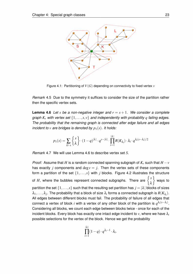
We investigate the event that after an edge failure the graph remains connected. Weconsider a fixed vertex v and partition the remaining vertex set depending on their con-nectivity to v (see Figure 4.1):
• Let E denote the bridges of G incident to v. Let I denote the connected componentcontaining v in G−E. Then S :=V (G)\V (I).• The vertex set K contains all vertices of the block of v (if v is contained in several
blocks, one arbitrarily chosen one is fixed for K)• Let H denote the connected component containing v in G− (K \ {v}). Then
T :=V (H)\S and L :=V (G)\ (V (H)∪K)
Given the partition of V into these vertex sets, we can derive independent formulas forthe probabilities of those sets. For the biconnected reliability it then remains to sum overall possible partitions of V and take into account that all edges between S, L and T andbetween S, T and K \{v} must fail.
Chapter 4: Special graph classes 23
vKS
T
L
Figure 4.1: Partitioning of V (G) depending on connectivity to fixed vertex v
Remark 4.5 Due to the symmetry it suffices to consider the size of the partition ratherthen the specific vertex sets.
Lemma 4.6 Let s be a non-negative integer and r = s+ 1. We consider a completegraph Kr with vertex set {1, . . . ,s,v} and independently with probability q failing edges.The probability that the remaining graph is connected after edge failure and all edgesincident to v are bridges is denoted by p1(s). It holds:
p1(s) = ∑λ`s
{sλ
}· (1−q)|λ | ·qs−|λ | ·
|λ |
∏i=1
R(Kλi) ·λi ·qλi(s−λi)/2
Remark 4.7 We will use Lemma 4.6 to describe vertex set S.
Proof: Assume that H is a random connected spanning subgraph of Kr such that H−vhas exactly j components and degv = j. Then the vertex sets of these componentsform a partition of the set {1, . . . ,s} with j blocks. Figure 4.2 illustrates the structure
of H, where the bubbles represent connected subgraphs. There are{
sλ
}ways to
partition the set {1, . . . ,s} such that the resulting set partition has j = |λ | blocks of sizesλ1, . . . ,λ j. The probability that a block of size λi forms a connected subgraph is R(Kλi).All edges between different blocks must fail. The probability of failure of all edges thatconnect a vertex of block i with a vertex of any other block of the partition is qλi(s−λi).Considering all blocks, we count each edge between blocks twice - once for each of theincident blocks. Every block has exactly one intact edge incident to v, where we have λi
possible selections for the vertex of the block. Hence we get the probability
|λ |
∏i=1
(1−q) ·qλi−1 ·λi.
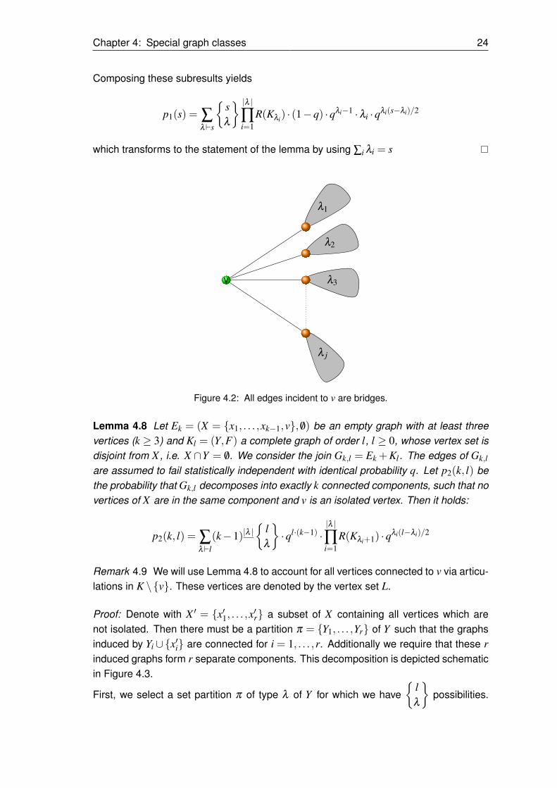
Chapter 4: Special graph classes 24
Composing these subresults yields
p1(s) = ∑λ`s
{sλ
} |λ |∏i=1
R(Kλi) · (1−q) ·qλi−1 ·λi ·qλi(s−λi)/2
which transforms to the statement of the lemma by using ∑i λi = s
v λ3
λ2
λ1
λ j
Figure 4.2: All edges incident to v are bridges.
Lemma 4.8 Let Ek = (X = {x1, . . . ,xk−1,v}, /0) be an empty graph with at least threevertices (k ≥ 3) and Kl = (Y,F) a complete graph of order l, l ≥ 0, whose vertex set isdisjoint from X , i.e. X ∩Y = /0. We consider the join Gk,l = Ek +Kl . The edges of Gk,l
are assumed to fail statistically independent with identical probability q. Let p2(k, l) bethe probability that Gk,l decomposes into exactly k connected components, such that novertices of X are in the same component and v is an isolated vertex. Then it holds:
p2(k, l) = ∑λ`l
(k−1)|λ |{
lλ
}·ql·(k−1) ·
|λ |
∏i=1
R(Kλi+1) ·qλi(l−λi)/2
Remark 4.9 We will use Lemma 4.8 to account for all vertices connected to v via articu-lations in K \{v}. These vertices are denoted by the vertex set L.
Proof: Denote with X ′ = {x′1, . . . ,x′r} a subset of X containing all vertices which arenot isolated. Then there must be a partition π = {Y1, . . . ,Yr} of Y such that the graphsinduced by Yi∪{x′i} are connected for i = 1, . . . ,r. Additionally we require that these rinduced graphs form r separate components. This decomposition is depicted schematicin Figure 4.3.
First, we select a set partition π of type λ of Y for which we have{
lλ
}possibilities.
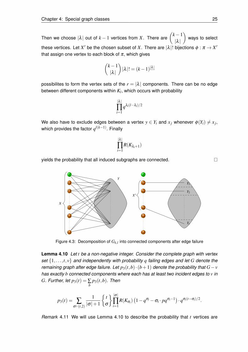
Chapter 4: Special graph classes 25
Then we choose |λ | out of k− 1 vertices from X . There are(
k−1|λ |
)ways to select
these vertices. Let X ′ be the chosen subset of X . There are |λ |! bijections φ : π → X ′
that assign one vertex to each block of π , which gives(k−1|λ |
)|λ |! = (k−1)|λ |
possibilites to form the vertex sets of the r = |λ | components. There can be no edgebetween different components within Kl , which occurs with probability
|λ |
∏i=1
qλi(l−λi)/2
We also have to exclude edges between a vertex y ∈ Yi and x j whenever φ(Yi) 6= x j,which provides the factor ql(k−1). Finally
|λ |
∏i=1
R(Kλi+1)
yields the probability that all induced subgraphs are connected.
v
x1
x2
xr
xr+1
xk-1
X
Yv
x′1
x′2
x′r
xr+1
xk-1
X ′
Y1
Y2
Yr
Figure 4.3: Decomposition of Gk,l into connected components after edge failure
Lemma 4.10 Let t be a non-negative integer. Consider the complete graph with vertexset {1, . . . , t,v} and independently with probability q failing edges and let G denote theremaining graph after edge failure. Let p3(t,b) · (b+1) denote the probability that G−vhas exactly b connected components where each has at least two incident edges to v inG. Further, let p3(t) = ∑
bp3(t,b). Then
p3(t) = ∑σ`(t,2)
1|σ |+1
{tσ
} |σ |∏i=1
R(Kσi)(1−qσi−σi · pqσi−1) ·qσi(t−σi)/2.
Remark 4.11 We will use Lemma 4.10 to describe the probability that t vertices are

Chapter 4: Special graph classes 26
connected to v via b additional blocks containing v besides K. The factor (b+ 1) ac-counts for the choice of K out of those (b+1) blocks.
Proof: Consider a fixed partition of {1, . . . , t}, such that each block contains at least twovertices and let ti denote the size of the ith block, i = 1, . . . ,b. The ti vertices form aconnected component in G− v and at least two edges towards v must remain intact.Additionally, the edges between different blocks must fail. Figure 4.4 illustrates thisevent. The probability for this event is:
p3(b, t,{ti}) :=b
∏i=1
R(Kti)︸ ︷︷ ︸ti connectedcomponent
·(1−qti− ti · (1−q)qti−1)︸ ︷︷ ︸
at least 2 edgesto v intact
· qti·(t−ti)/2︸ ︷︷ ︸ti disconnected from
all other blocks
Since until now we considered a fixed assignment of t. We now have to sum over allpossible assignments and consider permutations which result in the same graph.
p3(b, t) · (b+1) =1b!︸︷︷︸
permutationsof the ti
· ∑b∑
i=1ti=|t|
ti≥2
(t
t1, . . . tt
)︸ ︷︷ ︸
number of assignmentsof t towards {ti}
·p3(b, t,{ti})
By changing from the sum over all sums to number partitions where each block has atleast size two we get
p3(b, t) =1
b+1 ∑σ`(t,2)|σ |=b
{tσ
}p3(b, t,{σi})
=1
b+1 ∑σ`(t,2)|σ |=b
{tσ
} |σ |∏i=1
R(Kσi) ·(1−qσi−σi · (1−q)qσi−1) ·qσi·(t−σi)/2.
Hence, we get
p3(t) =∑b
p3(t,b)
=∑b
1b+1 ∑
σ`(t,2)|σ |=b
{tσ
} |σ |∏i=1
R(Kσi) ·(1−qσi−σi(1−q)qσi−1)qσi·(t−σi)/2
= ∑σ`(t,2)
1|σ |+1
{tσ
} |σ |∏i=1
R(Kσi) ·(1−qσi−σi(1−q)qσi−1)qσi·(t−σi)/2.
Chapter 4: Special graph classes 27
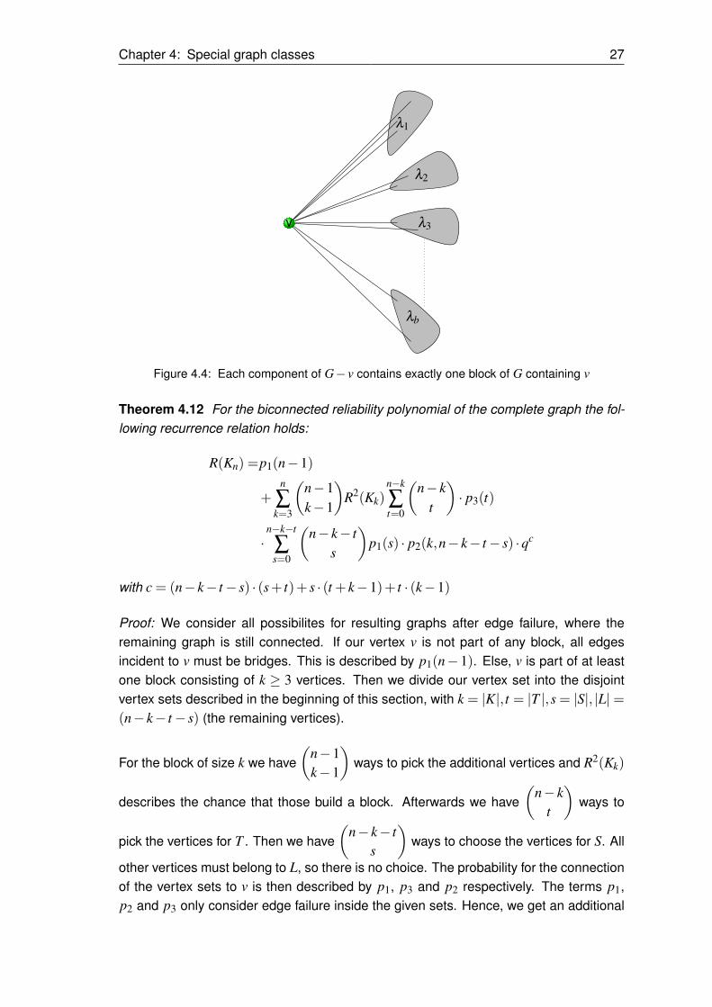
v λ3
λ2
λ1
λb
Figure 4.4: Each component of G− v contains exactly one block of G containing v
Theorem 4.12 For the biconnected reliability polynomial of the complete graph the fol-lowing recurrence relation holds:
R(Kn) =p1(n−1)
+n
∑k=3
(n−1k−1
)R2(Kk)
n−k
∑t=0
(n− k
t
)· p3(t)
·n−k−t
∑s=0
(n− k− t
s
)p1(s) · p2(k,n− k− t− s) ·qc
with c = (n− k− t− s) · (s+ t)+ s · (t + k−1)+ t · (k−1)
Proof: We consider all possibilites for resulting graphs after edge failure, where theremaining graph is still connected. If our vertex v is not part of any block, all edgesincident to v must be bridges. This is described by p1(n−1). Else, v is part of at leastone block consisting of k ≥ 3 vertices. Then we divide our vertex set into the disjointvertex sets described in the beginning of this section, with k = |K|, t = |T |,s = |S|, |L|=(n− k− t− s) (the remaining vertices).
For the block of size k we have(
n−1k−1
)ways to pick the additional vertices and R2(Kk)
describes the chance that those build a block. Afterwards we have(
n− kt
)ways to
pick the vertices for T . Then we have(
n− k− ts
)ways to choose the vertices for S. All
other vertices must belong to L, so there is no choice. The probability for the connectionof the vertex sets to v is then described by p1, p3 and p2 respectively. The terms p1,p2 and p3 only consider edge failure inside the given sets. Hence, we get an additional
Chapter 4: Special graph classes 28
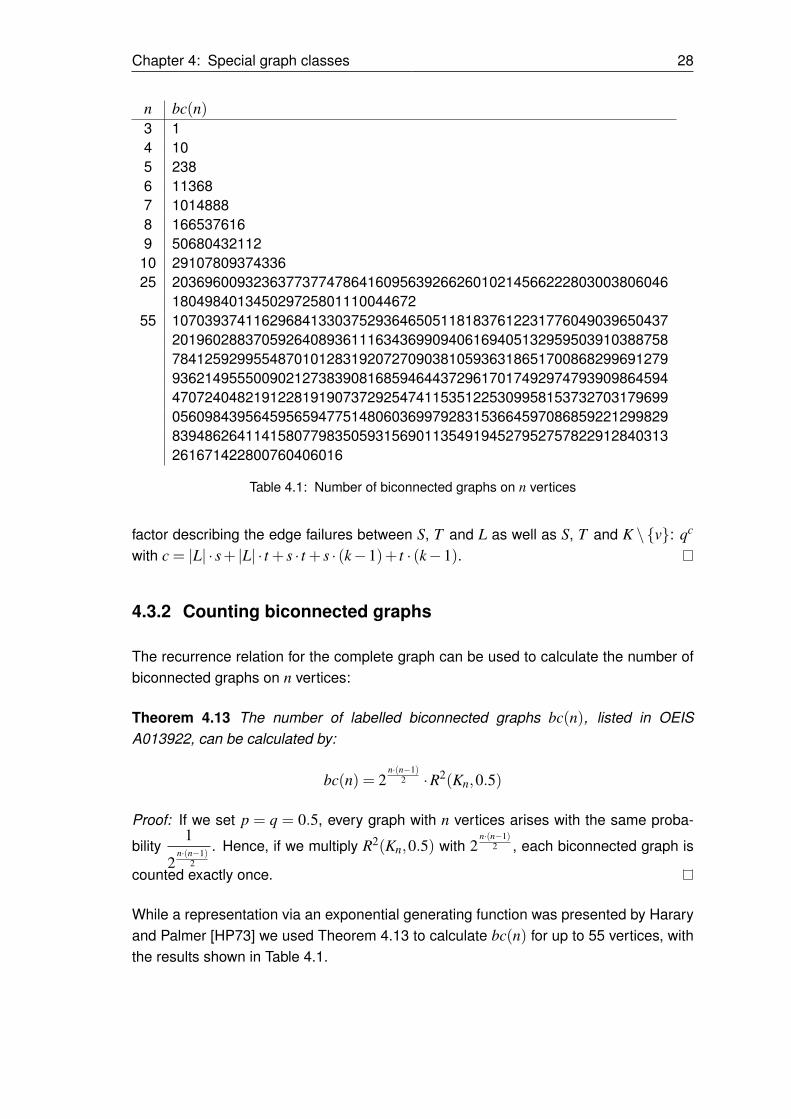
n bc(n)3 14 105 2386 113687 10148888 1665376169 50680432112
10 2910780937433625 2036960093236377377478641609563926626010214566222803003806046
18049840134502972580111004467255 1070393741162968413303752936465051181837612231776049039650437
201960288370592640893611163436990940616940513295950391038875878412592995548701012831920727090381059363186517008682996912799362149555009021273839081685946443729617017492974793909864594470724048219122819190737292547411535122530995815373270317969905609843956459565947751480603699792831536645970868592212998298394862641141580779835059315690113549194527952757822912840313261671422800760406016
Table 4.1: Number of biconnected graphs on n vertices
factor describing the edge failures between S, T and L as well as S, T and K \{v}: qc
with c = |L| · s+ |L| · t + s · t + s · (k−1)+ t · (k−1).
4.3.2 Counting biconnected graphs
The recurrence relation for the complete graph can be used to calculate the number ofbiconnected graphs on n vertices:
Theorem 4.13 The number of labelled biconnected graphs bc(n), listed in OEISA013922, can be calculated by:
bc(n) = 2n·(n−1)
2 ·R2(Kn,0.5)
Proof: If we set p = q = 0.5, every graph with n vertices arises with the same proba-
bility1
2n·(n−1)
2
. Hence, if we multiply R2(Kn,0.5) with 2n·(n−1)
2 , each biconnected graph is
counted exactly once.
While a representation via an exponential generating function was presented by Hararyand Palmer [HP73] we used Theorem 4.13 to calculate bc(n) for up to 55 vertices, withthe results shown in Table 4.1.
Chapter 4: Special graph classes 29
4.3.3 Running time analysis
For the running time analysis we assume that an can be calculated in a single timestep. Hardy and Ramanujan [HR18] and Uspensky [Usp20] showed, that the number ofpartitions of n, p(n), is asymptotically
p(n)∼ 14n√
3exp
(π
√2n3
).
Hence, it follows p(n) ∈O
(13,002
√n
n
). By applying this to our recurrence relation for
R2(Kn) we get the following theorem:
Theorem 4.14 R2(Kn) can be calculated via Theorem 4.12 in time O(n2 · 13,002√
n)
and space O(n6).
Proof: To calculate R2(Kn) via Theorem 4.12 we need to calculate the following subre-sults and store them:
• R(Ki) for i = 1, . . . ,n• p1(s) for s = 1, . . . ,n• p2(k, l) for k = 1, . . . ,n, l = 1, . . . ,n• p3(t) for t = 1, . . . ,n
Afterwards, to calculate R2(Ki) for i ∈ {1, . . . ,n} we need to sum over all choices for k,t, s and l which can be done in time O(n4). So to calculate all R2(Ki) after calculat-ing and storing our subresults (runtimes listed in table 4.2) we need O(n5) additionaloperations. R(Ki) for i = 1, . . . ,n can be calculated in time O(n2) via the recurrencerelation presented by Gilbert [Gil59]. To calculate p1(s) for a given s ≤ n we need tosum over all partitions and consider every block of the partition, which can be done in
O
(13,002
√s
s· s
)calculations. To store the result for a certain value of s as polynomial,
we have a polynomial of degree at mosts · (s+1)
2and since every edge can be intact or
can fail, which each may change coefficients by ±1, the highest coefficient has at mostlength O
(s2). Therefore p1(s) can be stored in space O
(s4).
By the same reasoning, we get that p2(k, l) for given k and l can be calculated in time
O(
13,002√
l)
and space O(l2 ·max{k, l}2).
For p3(t), the number of summands of ∑σ`(t,2)
is bounded above by p(t). Hence the run-
time for given t is in O(
13,002√
t)
. Since, due to the term1
b+1we can not guarantee
that the coefficients are integers, we could store the polynomial times (b+ 1) for eachvalue of b individually which therefore can be done in space O(t5).
Chapter 4: Special graph classes 30
Since s, k, l and t are all bounded above by n, all necessary subresults can be calcu-
lated in time O(
n2 ·13,002√
n)
and space O(n6).Since the summation over all subresults can be done in polynomial time and storing thebiconnected reliability polynomial for R2(Kk) for given k can be done in space O(k4),
the run-time of the complete algorithm is in O(
n2 ·13,002√
n)
and the space needed is
in O(n6).
Result runtime space # valuesR(Ki) O(i) O(i4) np1(s) O(13,002
√s) O(s4) n
p2(k, l) O(13,002√
l) O(l2 ·max{k, l}2) n2
p3(t) O(13,002√
t) O(t5) n
Table 4.2: Runtime and space requirement of the different subfunctions
4.3.4 Two-edge reliability polynomial
For the two-edge reliability polynomial the following recurrence relation was presentedby Reinwardt [Rei15]:
Theorem 4.15 For the two-edge reliability of the complete graph Kn, for short denotedby rn, holds:
rn = 1−∑λ`n
{nλ
} |λ |∏i=1
qλi(n−λi)
2 ∑σ`λi
σ 6=(n)
{λi
σ
}(1−q)|σ |−1q1−|σ |tσ
|σ |
∏j=1
qσ j(λi−σ j)
2 rσ j
where tσ denotes the number of spanning trees of λi connecting the components of σ .
Proof: The proof is by considering all events (therefore "1−" after solving for rn) of edgefailure and considering all connected components (λi) and their respective two-edgeconnected components (σ j) and calculating the probability for those. For the full proof,see Reinwardt [Rei15].
By limiting to the event that the resulting graph is connected, this formula simplies whilethe given proof by Reinwardt still holds:
Theorem 4.16 For the two-edge reliability polynomial of Kn, R2−ec(Kn), holds:
R2−ec(Kn) =R(Kn)− ∑σ`n
σ 6=(n)
{nσ
}(1−q)|σ |−1q1−|σ |tσ
|σ |
∏j=1
qσ j(n−σ j)
2 R2−ec(Kσ j)
Chapter 4: Special graph classes 31
Alternatively we can as well again consider a fixed vertex v ∈ V and get the followingrecurrence relation:
Theorem 4.17 For the two-edge reliability polynomial of Kn the following recurrencerelation holds:
R(Kn) =n
∑k=1
(n−1k−1
)R2−ec(Kk) ·qk(n−k) · ∑
λ`n−k
{n− k
λ
}(1−q
q
)|λ |·|λ |
∏i=1
R(Kλi) · k ·λi ·qλi(n−k−λi)/2.
Proof: We consider a fixed vertex v ∈ V and the event that the graph G, resulting afteredge failure, remains connected. Then v is in a two-edge connected component K ofsize k ≥ 1. Consider the connected components of G−K. They form a partitioning ofthe vertex set V \K with block size distribution λ , which is illustrated in Figure 4.5. Foreach of the blocks, the following properties hold:
• the block is connected• exactly one edge to K is intact in G• edges between different blocks fail
Hence, for the ith block we get the following probability independent of the other blocks:
R(Kλi)︸ ︷︷ ︸block connected
·k ·λi · (1−q) ·qk·λi−1︸ ︷︷ ︸exactly 1 edge to K
· qλi(n−k−λi)/2︸ ︷︷ ︸edges to other blocks fail
We have to sum over all block size distributions of set partitions of the vertex set V \K,hence
∑λ`n−k
{n− k
λ
}︸ ︷︷ ︸
number of set partitionswith block size distribution λ
|λ |
∏i=1
R(Kλi) · k λi · (1−q) ·qk·λi−1 ·qλi(n−k−λi)/2
= ∑λ`n−k
{n− k
λ
}· (1−q)|λ | ·qk·(n−k)−|λ | ·
|λ |
∏i=1
R(Kλi) · k λi ·qλi(n−k−λi)/2.
The probability for K to be the two-edge-connected component of v is given by(n−1k−1
)︸ ︷︷ ︸
choices for K
· R2−ec(Kk)︸ ︷︷ ︸K two-edge-connected
.
Summing over all possible sizes k of K yields the considered event that the graph isconnected and therefore R(Kn) and the theorem holds.It is noteworthy that the recurrence relation gives R2−ec(K1) = 1 and R2−ec(K2) = 0,
Chapter 4: Special graph classes 32
hence, since the λi are connected to K via bridges, unlike for the biconnected reliability,we do not need a special case in the event that all edges incident to v form bridges.
K v λ3
λ2
λ1
λ j
Figure 4.5: Partitioning of V (Kn) into the two-edge connected component K containing v andconnected components λi connected to v via bridges
4.4 Complete bipartite graphs Ka,b
For certain (small) choices of a, we can derive explicit formulas for Ka,b by analyzingwhat different vertex degree distributions of B after edge failure result in biconnectedgraphs.It follows immidiatly, that
R2(K1,b) = 0 and
R2(K2,b) = p2b.
4.4.1 Complete bipartite graphs K3,b
Theorem 4.18 For the complete bipartite graph K3,b, b≥ 3 holds
R2(K3,b) = (p3 +3qp2)b−3 ·b · p3(qp2)b−1− (qp2)b · (3 ·2b−3).
Proof: Denote the vertices of A by u,v,w. For the remaining graph G to be biconnected,every vertex of B need to have at least degree 2. The degree-2-vertices of B can bepartitioned into three classes depending on their neighbourhood. Then in the followingdisjoint cases the graph is biconnected:

Chapter 4: Special graph classes 33
1. At least two vertices of B have degree 3.2. Exactly one vertex of B has degree 3 and every vertex of A is adjacent to at least
one degree-2-vertex of B.3. All vertices of B have degree 2 and all three classes of degree-2-vertices are
prevalent.
Case 1
The probability for this case is: P1 :=b∑
k=2
(bk
)(p3)k ·
(3qp2)b−k
, where k denotes the
number of vertices of degree 3 of B.By applying the Binomial theorem, we get
P1 =(
p3 +3qp2)b−b · p3 (3qp2)b−1−(3qp2)b
.
Case 2The probability for this case is
P2 := b · p3 ·(qp2)b−1 · (3b−1−3)
where the (3b−1−3) regards that all assignments of the degree-2-vertices in the threesubclasses are valid, unless all vertices get assigned to the same class.Case 3The probability for this case is
P3 :=(qp2)b · (3b−3 ·2b +3),
where the factor (3b−3 ·2b+3) accounts for an arbitrary assignment towards the threeclasses such that all are non-empty.
The theorem then follows by R2(K3,b) = P1 +P2 +P3.
4.4.2 Complete bipartite graphs K4,b
Theorem 4.19 For the complete bipartite graph K4,b, b≥ 4 holds
R2(K4,b) =(
p4 +4p3q+6p2q2)b−4b · p4 ·(
p3q+3p2q2)b−1
−3b · p4 ·(2p2q2)b−1
+12b · p4 ·(
p2q2)b−1
+6b(b−1) · (p3q)2 · (p2q2)b−2−12b · p3q(p3q+3p2q2)b−1
+24b · p3q(2p2q2)b−1−12b · p3q(p2q2)b−1−12(p3q+4p2q2)b
+8(p3q+3p2q2)b +(p2q2)b · (20 ·3b−27 ·2b +12).
Proof: We again investige all possible vertex degree distributions of B, which result in a
Chapter 4: Special graph classes 34
biconnected graph.
Case 1: At least two vertices have degree 4.
P1 :=b∑
k=2
(bk
)(p4)k · (4qp3 +6p2q2)b−k
Case 2: Exactly one vertex has degree 4.
Case 2.1: there are at least two classes of degree-3-vertices which are non-empty.
P2.1 := b · p4 ·b−1∑
k=2
(b−1
k
)· (p3q)k · (4k−4) · (6p2q2)b−1−k
Case 2.2: There is exactly one class of degree.3-vertices.
P2.2 := b · p4 ·b−1∑
k=1
(b−1
k
)·4 · (p3q)k · (p2q2)b−1−k (6b−1−k−3b−1−k)︸ ︷︷ ︸
reaching missingvertex by degree-2-vertices
Case 2.3: There is no degree-3-vertex.Then there need to be at least three classes of degree-2-vertices (otherwisethe degree-4-vertex is an articulation) and every vertex of A needs to beadjacent to a degree-2-vertex.
P2.3 := b · p4 · (p2q2)b−1 ·
6b−1−4 ·3b−1 +6︸ ︷︷ ︸every a-vertex reached
− (3 ·2b−1−6)︸ ︷︷ ︸short-cycles
reaching all a-vertices
Case 3: There are at least three classes of degree-3-vertices.
P3 :=b∑
k=3
(bk
)(p3q)k · (4k−6 ·2k +8) · (6p2q2)b−k
Case 4: There are exactly two classes of degree-3-vertices.
Case 4.1: Both classes have at least two vertices.
P4.1 :=b∑
k=4
(bk
)·6 · (p3q)k · (2k−2−2k) · (6p2q2)b−k
Case 4.2: One class has exactly one vertex.The a-vertex adjacent to only one degree-3-vertex then needs to be adjacentto a degree-2-vertex.
P4.2 :=b∑
k=3
(bk
)·4 ·3 · k · (p3q)k · (p2q2)b−k · (6b−k−3b−k)
Case 4.3: Both classes have exactly one vertex.
Case 4.3.1: The two a-vertices with only one degree-3-neighbour have acommon degree-2-neighbour.
P4.3.1 :=(
b2
)·4 ·3 · (p3q)2 · (p2q2)b−2 · (6b−2−5b−2)
Case 4.3.2: The two a-vertices do not have a common degree-2-neighbourbut are both adjacent to at least one degree-2-vertex.
Chapter 4: Special graph classes 35
P4.3.2 :=(
b2
)·4 ·3 · (p3q)2 · (p2q2)b−2 · (5b−2−2 ·3b−2 +1)
We get
P4.3 := P4.3.1 +P4.3.2 =
(b2
)·12 · (p3q)2 · (p2q2)b−2 · (6b−2−2 ·3b−2 +1).
Case 5: There is exactly one class of degree-3-vertices which has at least two vertices.Then the remaining a-vertex has to be adjacent to two different classes of degree-2-vertices.
P5 :=b∑
k=2
(bk
)·4 · (p3q)k · (p2q2)b−k(6b−k−3 ·4b−k +2 ·3b−k)
Case 6: There is exactly one degree-3-vertex.
Case 6.1: For the remaining a-vertex all three classes of adjacent degree-2-verticesare non-empty.P6.1 := 4b · p3q · (p2q2)b−1 · (6b−1−3 ·5b−1 +3 ·4b−1−3b−1)
Case 6.2: For the remaining a-vertex exactly two classes of adjacent degree-2-vertices are non-empty.Then the second a-vertex of the missing class must be reached by the re-maining degree-2-vertices.P6.2 := 4b · p3q · (p2q2)b−1 ·3 · (5b−1−2 ·4b−1 +2 ·2b−1−1)
We get
P6 := P6.1 +P6.2 = 4t · p3q · (p2q2)b−1 · (6b−1−3 ·4b−1−3b−1 +6 ·2b−1−3).
Case 7: All b-vertices have degree 2.
Case 7.1: All classes of degree-2-vertices are non-empty.P7.1 := (p2q2)b · (6b−6 ·5b +15 ·4b−20 ·3b +15 ·2b−6)
Case 7.2: Exactly one class is empty.P7.2 := (p2q2)b ·6 · (5b−5 ·4b +10 ·3b−10 ·2b +5)
Case 7.3: Exactly two classes are empty, which have no a-vertex in common.P7.3 := (p2q2)b ·3 · (4b−4 ·3b +6 ·2b−4)
Therefore we get
P7 := P7.1 +P7.2 +P7.3 = (p2q2)b · (6b−12 ·4b +28 ·3b−27 ·2b +12).
Altogether, we get
R2(K4,t) = P1 +P2.1 +P2.2 +P2.3 +P3 +P4.1 +P4.2 +P4.3 +P5 +P6 +P7.
Chapter 4: Special graph classes 36
The theorem follows by applying the Binomial theorem to the sums over k.
Conclusion:
By distinction of possible vertex degrees, it is possible to get an explicitformula for every fixed a. Unfortunately, the number of distinct successcases, which need to be considered, becomes vast already for relativelysmall a. Hence, in the following section a recursive formula for arbitrary awill be developed.
4.4.3 A recurrence relation for the biconnected reliabilitypolynomial of Ka,b
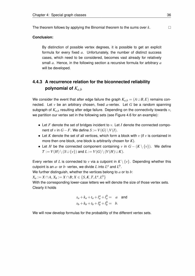
We consider the event that after edge failure the graph Ka,b = (A∪B,E) remains con-nected. Let v be an arbitrary chosen, fixed a-vertex. Let G be a random spanningsubgraph of Ka,b resulting after edge failure. Depending on the connectivity towards v,we partition our vertex set in the following sets (see Figure 4.6 for an example):
• Let F denote the set of bridges incident to v. Let I denote the connected compo-nent of v in G−F . We define S :=V (G)\V (I).• Let K denote the set of all vertices, which form a block with v (if v is contained in
more then one block, one block is arbitrarily chosen for K).• Let H be the connected component containing v in G− (K \ {v}). We define
T :=V (H)\ (S∪{v}) and L :=V (G)\ (V (H)∪K).
Every vertex of L is connected to v via a cutpoint in K \ {v}. Depending whether thiscutpoint is an a- or b- vertex, we divide L into La and Lb.We further distinguish, whether the vertices belong to a or to b:Xa := X ∩A, Xb := X ∩B; X ∈ {S,K,T,La,Lb}With the corresponding lower-case letters we will denote the size of those vertex sets.Clearly it holds
sa + ka + ta + laa + lb
a = a and
sb + kb + tb + lab + lb
b = b.
We will now develop formulas for the probability of the different vertex sets.
Chapter 4: Special graph classes 37
v
K
TS
La
Lb
Figure 4.6: Vertex partitioning depending on connectivity to fixed vertex v after edge failure
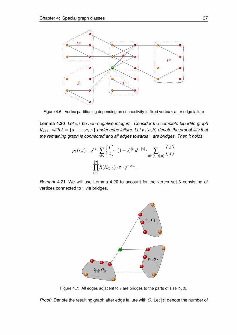
Lemma 4.20 Let s, t be non-negative integers. Consider the complete bipartite graphKs+1,t with A = {a1, . . . ,as,v} under edge failure. Let p1(a,b) denote the probability thatthe remaining graph is connected and all edges towards v are bridges. Then it holds
p1(s, t) =qs·t ·∑τ`t
{tτ
}· (1−q)|τ|qt−|τ| · ∑
σ�(s,|τ|,0)
(sσ
)
·|τ|
∏i=1
R(Kσi,τi) · τi ·q−σiτi.
Remark 4.21 We will use Lemma 4.20 to account for the vertex set S consisting ofvertices connected to v via bridges.
v
τ1,σ1
τ2,σ2
τ|τ|,σ|τ|
Figure 4.7: All edges adjacent to v are bridges to the parts of size τi,σi.
Proof: Denote the resulting graph after edge failure with G. Let |τ| denote the number of

Chapter 4: Special graph classes 38
components of G−v and τi and σi denote the number of b- and a- vertices respectivelyin the ith connected component (see Figure 4.7 for the structure of G). Note, that eachcomponent must contain a b-vertex (τi≥ 1) while it is possible that a component consistssolely of one b-vertex and no a-vertices (σi ≥ 0). Given the size of the components,
we have{
tτ
}ways to assign the b-vertices to the components and afterwards we can
choose the a-vertices in(
sσ
)ways. For every component the following properties need
to hold:
• The component must be connected intrinsic.• All edges to the other components fail.• One edge to v is intact, the others fail.
Since these properties describe disjoint edge sets, the probabilities are independentand can be multiplied. The probability for that is:
|τ|
∏i=1
R(Kσi,τi)︸ ︷︷ ︸connected
·τi · (1−q)qτi−1︸ ︷︷ ︸one edge tov
· qσi·(t−τi)︸ ︷︷ ︸edges between different
components fail
We sum over all possible sizes for τi and σi.By using t = ∑i τi, ∑i σi(t− τi) = st−∑i σiτi the result follows.
Lemma 4.22 Consider the complete bipartite graph Ks+1,t with A= {a1, . . . ,as,v} underedge failure. Let p2(b,s, t) denote the probability that the remaining graph is connectedand v is contained in exactly b blocks and no edges incident to v are bridges. Further
let p2(s, t) := ∑b
p2(b,s, t)b+1
. Then it holds
p2(s, t) = qs·t ·∑σ`s
{sσ
}1
|σ |+1 ∑τ�(t,|σ |,2)
(tτ
)
·|σ |
∏i=1
R(Kσi,τi) · (1−qτi− τi(1−q)qτi−1) ·q−σi·τi.
Remark 4.23 We will use this lemma to describe the connectivity of the vertex set T to
v. The term1
b+1accounts for the different choices of K out of b+1 blocks.
Proof: Denote the remaining graph after edge failure with G. Since no edges incidentto v are bridges, G− v decomposes in b connected components (where the number ofvertices is denoted by σi and τi), all of them having at least two intact edges towards vin G. Since v is adjacent only to b-vertices and these b-vertices must be connected via
Chapter 4: Special graph classes 39
an a-vertex in the component, it follows σi ≥ 1 and τi ≥ 2 for all i. We have{
sσ
}ways
to assign the a-vertices to the components and(
tτ
)ways to choose the b-vertices. For
every component the following properties need to hold:
• The components are connected intrinsic.• All edges between different components fail.• At least 2 edges to v must remain intact.
The probability for that is
b
∏i=1
R(Kσi,τi)︸ ︷︷ ︸connected
·(1−qτi− τi(1−q)qτi−1)︸ ︷︷ ︸
at least 2 edges to v
· qσi(t−τi)︸ ︷︷ ︸edges between different
components fail
.
It remains to sum over all sizes of τi and σi. By using ∑i σi = s, we get
p2(b,s, t) = ∑σ`s|σ |=b
{sσ
}· ∑
τ�(t,|σ |,2)
(tτ
)
·qs·t ·b
∏i=1
R(Kσi,τi) · (1−qτi− τi(1−q)qτi−1) ·q−σi·τi.
The result then follows immidiatly from p2(s, t) := ∑b
p2(b,s, t)b+1
.
Lemma 4.24 Consider the complete bipartite graph Ks,t+k with B= {t1, . . . , tt︸ ︷︷ ︸T
,k1, . . . ,kk︸ ︷︷ ︸K
}.
Let p3(k,s, t) describe the probability that after edge failure the remaining graph decom-poses into exactly k connected components and no two vertices of K are in the samecomponent. Then it holds:
p3(k,s, t) = ∑σ`s
{sσ
}k|σ | · ∑
τ�(t,|σ |,0)
(tτ
)·qs·t+s·(k−1) ·
|σ |
∏i=1
R(Kσi,τi+1) ·q−σi·τi.
Remark 4.25 We will use this to describe the vertex sets Ls and Lt which are connectedvia an articulation in K \{v}.
Proof: Let |σ | denote the number of vertices of K which are not isolated after edgefailure. Let σi and τi denote the number of vertices of A and T respectively connected
to the ith non-isolated vertex of K. Hence, it holds: σi ≥ 1, τi ≥ 0. We have{
sσ
}ways to choose the assignment of A towards the connected components. Afterwards
Chapter 4: Special graph classes 40
we have k|σ | ways to assign the corresponding non-isolated vertices of K and(
tτ
)ways
to choose the assignment of the vertices of T . The components must be connected andall edges towards other components need to fail. We get
|σ |
∏i=1
R(Kσi,τi+1) ·qσi·(k−1) ·qσi·(t−τi).
It remains to sum over all sizes of σi and τi.
Theorem 4.26 For the complete bipartite graph Ka,b, a,b≥ 2 holds
R(Ka,b) =p1(a−1,b)
+a
∑ka=2
b
∑kb=2
(a−1ka−1
)(bkb
)R2(Kka,kb)
·a−ka
∑ta=0
b−kb
∑tb=0
(a− ka
ta
)(b− kb
tb
)p2(ta, tb)
·a−ka−ta
∑laa=0
b−kb−tb
∑lab=0
(a− ka− ta
laa
)(b− kb− tb
lab
)p3(ka−1, la
b , laa)
·a−ka−ta−la
a
∑lba=0
b−kb−tb−lab
∑lbb=0
(a− ka− ta− la
alba
)(b− kb− tb− la
blbb
)· p3(kb, lb
a , lbb) · p1(sa,sb) ·qc
with sa = a− ka− ta− laa− lb
a ; sb = b− kb− tb− lab− lb
b and
c =sa · (b− sb)+ sb · (a−1− sa)+ ta · (b− tb− sb)+ tb · (a−1− ta− sa)
+ laa · lb
b + lab · l
ba + la
b + laa · kb + lb
b · ka.
Proof: We consider the event that after edge failure the remaining graph remains con-nected. We consider a fixed a-vertex v. If v is not within a block, all edges incidentto v must be bridges and the probability can be described by p1(a− 1,b). Otherwise,we partition the vertex set depending on the connectivity towards v in the vertex setsS,K,T,Lb,La described in the beginning of this section. Given the size of the vertex
sets, we have(
a−1ka−1, ta, la
a , lba ,sa
)choices for the a-vertices without v into the different
sets and(
bkb, tb, la
b , lbb ,sb
)choices for the b-vertices. The connectivity of the vertex set
K is then described by R2(Kka,kb), the connectivity of S is described by p1(sa,sb), theconnectivity of T is described by p2(ta, tb) and the connectivity La and Lb is describedby p3(ka−1, la
b , laa) and p3(kb, lb
a , lbb) respectively. It remains to consider the necessary
edge failures between the different sets with qc.
Chapter 4: Special graph classes 41
Remark 4.27 We can easily derive a recurrence relation from Theorem 4.26 by rear-ranging terms.
4.4.4 Two-edge connected reliability polynomial of Ka,b
For the two-edge connected reliability polynomial of the complete bipartite graph weconsider the event that the remaining graph after edge failure is connected. We considera fixed a-vertex v and partition the vertex set depending on the connectivity to v.
Theorem 4.28 For the two-edge connected reliability polynomial of Ka,b holds
R(Ka,b) =p1(a−1,b)
+a
∑ka=2
b
∑kb=2
(a−1ka−1
)(bkb
)R2−ec(Kka,kb)
·a−ka
∑la=0
(a− ka
la
)(kb(1−q)qkb−1)la
b−kb
∑lb=0
(b− kb
lb
)(ka(1−q)qka−1)lb
· p2(ka,kb,a− ka− la,b− kb− lb) ·qc
with c = la(b− kb− lb)+ lb(a− ka), p1 defined in Lemma 4.20 and
p2(ka,kb,sa,sb) :=qkbsa+kasb+sasb ∑σ`sa
∑τ�(sb,|σ |)
{sa
σ
}(sb
τ
)· (1−q)|σ |q−|σ |
·|σ |
∏i=1
R(Kσi,τi) · (σikb + τika) ·q−σi·τi.
Proof: We consider the event that the remaining graph after edge failure is connected.Let v be a fixed a-vertex. Then the following events might occur:
• The vertex v is not in a two-edge connected component.This occurs if and only if v is not part of a block, so the probability for this event canbe described exactly as for the biconnected reliability: p1(a− 1,b) as describedin Lemma 4.20.• The vertex v is in a two-edge connected component.
Then we distinguish the following vertex sets (see Figure 4.8 for an example):
– We denote by K the vertices of this two-edge connected component.– Let H := G−K. Then let L denote the set of isolated vertices of H and S
denote the vertices in components of size ≥ 2 (which therefore have at leastone a- and b-vertex).
Let Ka and Kb denote the vertices of K which are a-vertices and b-vertices, respectively.
Chapter 4: Special graph classes 42
Analogously, define La, Lb, Sa and Sb. Let the corresponding lower case letters denotethe sizes of these sets. Then it clearly holds
a = ka + la + sa and
b = kb + lb + sb.
We consider a fixed assignment of the vertices towards the sets K, L and S. Then theprobability for K to be a two-edge connected component is R2−ec(Kka,kb).Since the vertices of L are isolated in H, every vertex of La (Lb) must be of degree 1and the operating edge is incident to a vertex of Kb (Ka). The probability for this edgefailure towards K is
(kb · (1−q) ·qkb−1)la and(
ka · (1−q) ·qka−1)lb respectively.For the set S now consider a certain assignment of the vertices towards the connectedcomponents in H. Let |σ | denote the number of those components and σ1, . . . ,σ|σ |the sizes of the a-vertex sets of the components. Let τ1, . . . ,τ|σ | be the sizes of thecorresponding b-vertex sets. For every component, the following properties need tohold: Exactly one edge towards K needs to be operating, the components must beconnected intrinsically and all edges between different components need to fail. Theprobability for this is
(1−q)|σ |qkbsa+kasb−|σ |︸ ︷︷ ︸every component has exactly
one operating edge to K
·|σ |
∏i=1
R(Kσi,τi)︸ ︷︷ ︸intrinsicallyconnected
· (σikb + τika)︸ ︷︷ ︸choices for
operating edge to K
· qσi(sb−τi)︸ ︷︷ ︸all edges to othercomponents fail
.
By considering all assignments of S towards the components, we get the term describedby p2(ka,kb,sa,sb).All edges between S and L and all edges in L need to fail, which results in the term qc
with c = la(b− kb− lb)+ lb(a− ka− la)+ la · lb.It remains to sum over all assignments to K, L and S and combining the correspondingsubresults.
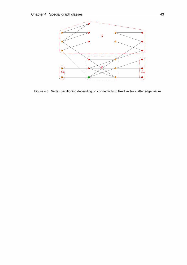
Chapter 4: Special graph classes 43
v
KLaLb
S
Figure 4.8: Vertex partitioning depending on connectivity to fixed vertex v after edge failure
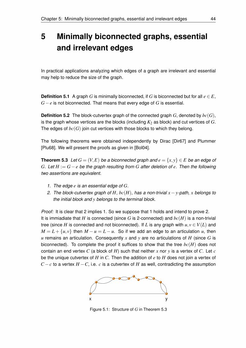
Chapter 5: Minimally biconnected graphs, essential and irrelevant edges 44
5 Minimally biconnected graphs, essentialand irrelevant edges
In practical applications analyzing which edges of a graph are irrelevant and essentialmay help to reduce the size of the graph.
Definition 5.1 A graph G is minimally biconnected, if G is biconnected but for all e ∈ E,G− e is not biconnected. That means that every edge of G is essential.
Definition 5.2 The block-cutvertex graph of the connected graph G, denoted by bc(G),is the graph whose vertices are the blocks (including K2 as block) and cut vertices of G.The edges of bc(G) join cut vertices with those blocks to which they belong.
The following theorems were obtained independently by Dirac [Dir67] and Plummer[Plu68]. We will present the proofs as given in [Bol04].
Theorem 5.3 Let G = (V,E) be a biconnected graph and e = {x,y} ∈ E be an edge ofG. Let H := G− e be the graph resulting from G after deletion of e. Then the followingtwo assertions are equivalent.
1. The edge e is an essential edge of G.2. The block-cutvertex graph of H, bc(H), has a non-trivial x− y-path, x belongs to
the initial block and y belongs to the terminal block.
Proof: It is clear that 2 implies 1. So we suppose that 1 holds and intend to prove 2.It is immiadiate that H is connected (since G is 2-connected) and bc(H) is a non-trivialtree (since H is connected and not biconnected). If L is any graph with u,v ∈V (L) andM = L+ {u,v} then M− u = L− u. So if we add an edge to an articulation u, thenu remains an articulation. Consequently x and y are no articulations of H (since G isbiconnected). To complete the proof it suffices to show that the tree bc(H) does notcontain an end vertex C (a block of H) such that neither x nor y is a vertex of C. Let cbe the unique cutvertex of H in C. Then the addition of e to H does not join a vertex ofC− c to a vertex H−C, i.e. c is a cutvertex of H as well, contradicting the assumption
x y
Figure 5.1: Structure of G in Theorem 5.3
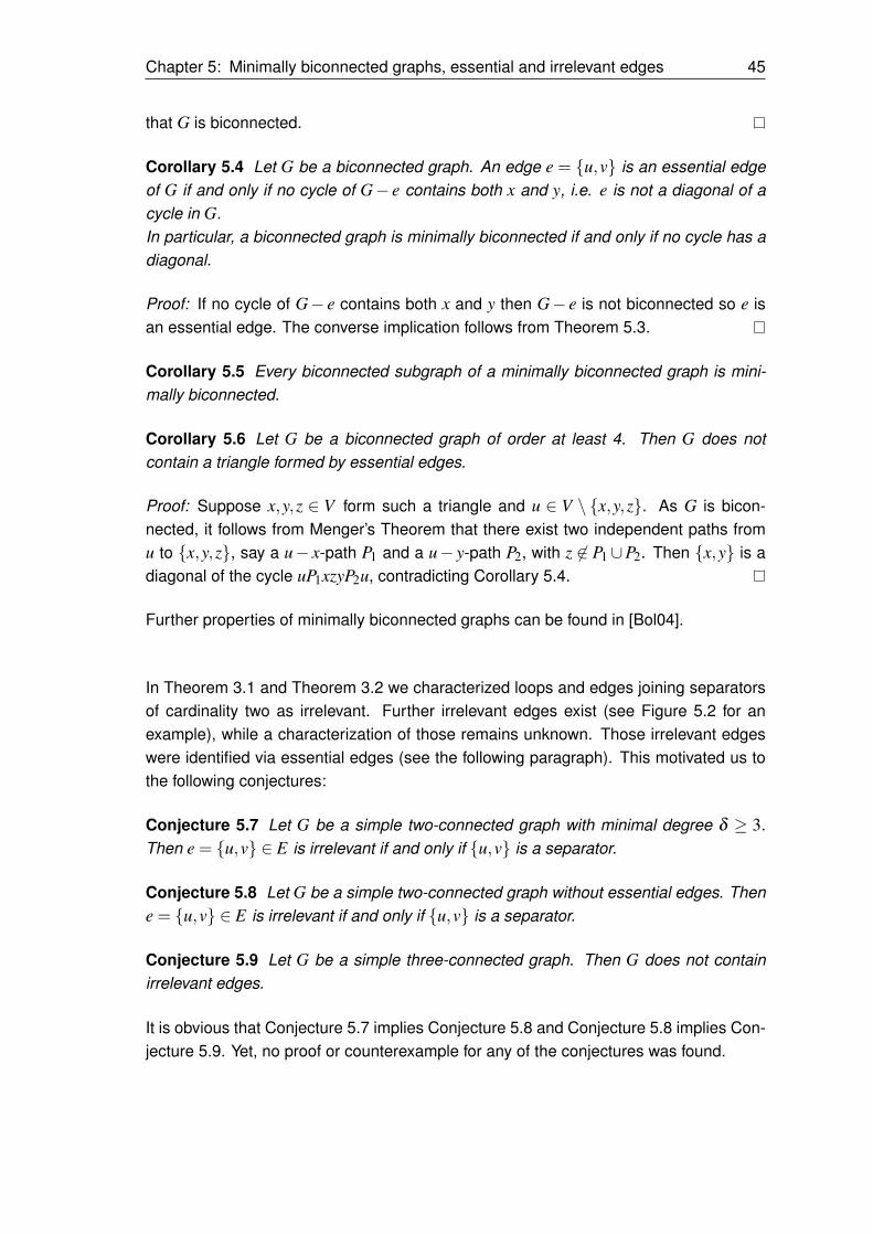
Chapter 5: Minimally biconnected graphs, essential and irrelevant edges 45
that G is biconnected.
Corollary 5.4 Let G be a biconnected graph. An edge e = {u,v} is an essential edgeof G if and only if no cycle of G− e contains both x and y, i.e. e is not a diagonal of acycle in G.In particular, a biconnected graph is minimally biconnected if and only if no cycle has adiagonal.
Proof: If no cycle of G− e contains both x and y then G− e is not biconnected so e isan essential edge. The converse implication follows from Theorem 5.3.
Corollary 5.5 Every biconnected subgraph of a minimally biconnected graph is mini-mally biconnected.
Corollary 5.6 Let G be a biconnected graph of order at least 4. Then G does notcontain a triangle formed by essential edges.
Proof: Suppose x,y,z ∈ V form such a triangle and u ∈ V \ {x,y,z}. As G is bicon-nected, it follows from Menger’s Theorem that there exist two independent paths fromu to {x,y,z}, say a u− x-path P1 and a u− y-path P2, with z 6∈ P1∪P2. Then {x,y} is adiagonal of the cycle uP1xzyP2u, contradicting Corollary 5.4.
Further properties of minimally biconnected graphs can be found in [Bol04].
In Theorem 3.1 and Theorem 3.2 we characterized loops and edges joining separatorsof cardinality two as irrelevant. Further irrelevant edges exist (see Figure 5.2 for anexample), while a characterization of those remains unknown. Those irrelevant edgeswere identified via essential edges (see the following paragraph). This motivated us tothe following conjectures:
Conjecture 5.7 Let G be a simple two-connected graph with minimal degree δ ≥ 3.Then e = {u,v} ∈ E is irrelevant if and only if {u,v} is a separator.
Conjecture 5.8 Let G be a simple two-connected graph without essential edges. Thene = {u,v} ∈ E is irrelevant if and only if {u,v} is a separator.
Conjecture 5.9 Let G be a simple three-connected graph. Then G does not containirrelevant edges.
It is obvious that Conjecture 5.7 implies Conjecture 5.8 and Conjecture 5.8 implies Con-jecture 5.9. Yet, no proof or counterexample for any of the conjectures was found.
Chapter 5: Minimally biconnected graphs, essential and irrelevant edges 46
e f
Figure 5.2: Graph with irrelevant edges e and f which do not join separators of cardinality two
For practical applications we can delete all edges e with R2(G) = R2(G− e). All irrel-evant edges fulfill this property. Further, edges having probability one (by default orafter applying reductions/decomposition formula), may result in other edges becomingdispensable:
Theorem 5.10 Let G= (V,E) be a probabilistic graph. Let F ⊆E be a circle of fail-proofedges and W ⊆ V the vertices incident to F . Then for all edges e = {u,v} ∈W 2 \Fholds:
R2K(G) = R2
K(G− e)
Further, if W is a separator of G, then it holds:
R2(G) = R2(G1) ·R2(G2)
Proof: The biconnected reliability can be expressed via success sets as described inEquation 2.1. All success sets A with F 6⊆ A account with zero in this sum due to theterm (1− p f ) for some f ∈ F . Hence we could limit the set of success sets to thosecontaining F and considering minimal success sets of those. Then e is in no minimalsuccess set, since two disjoint paths from u to v can always be obtained via F .If W is a separator, then x∈V1 and y∈V2 can only be in the same block if there exist twodisjoint paths traversing through W . Denote these paths as xP1w1Q1y and xP2w2Q2y.Then xP1w1F ′w2P2x with F ′ ⊆ F is a cycle in G1 and hence x, w1 and w2 are in thesame block in G1. The same holds for y in G2. Therefore all vertices of V are in thesame block in G if all vertices of V1 are in the same block in G1 and all vertices of V2 arein the same block of V2. If all vertices are in the same block in G1 and G2, they are inthe same block in G and hence equality holds.
Chapter 6: Summary and Prospect 47
6 Summary and Prospect
Since the underlying problem is NP-hard, algorithms for general graphs are likely toremain exponentiell. For certain graph classes however, algorithms were found whichoutperform complete enumeration of all states. Further, we presented some reductionswhich can reduce the size of a considered graph or resulting graphs during decomposi-tion and extended some of those to other reliability measures. For some applications itmay be sufficient to know, whether the reliability surpasses a critical value. Hence, theanalysis of lower and upper bounds of the biconnected reliability might become a topicof interest in following studies. Additionally we analyzed undirected networks. For prac-tical applications some connections allow only one-sided communication. The analysisof directed networks might be appropriate. Especially the analysis of acyclic graphs andthe conversion of an undirected to a directed network with the same reliability seem fea-sible tasks. Further analysis considering k-connectivity of probabilistic graphs or transfercapacities may be part of upcoming studies as well.
Bibliography 48
Bibliography
[Bol04] Béla Bollobás. Extremal graph theory. Courier Corporation, 2004.
[BR11] Suresh Badarla and Raghavan Rama. Note on minimally k-connected graphs.arXiv preprint arXiv:1103.4686, 2011.
[Col91] Charles J. Colbourn. Combinatorial aspects of network reliability. Annals ofOperations Research, 33(1):1–15, 1991.
[dF01] Babette L. E. de Fluiter. Algorithms for graphs of small treewidth. PhD thesis.University Utrecht, 2001.
[Dir66] Gabriel A. Dirac. Short proof of Menger’s graph theorem. Mathematika,13(1):42–44, 1966.
[Dir67] Gabriel A. Dirac. Minimally 2-connected graphs. Journal für die reine undangewandte Mathematik, 228(204216):2, 1967.
[Gil59] Edgar N. Gilbert. Random graphs. The Annals of Mathematical Statistics,pages 1141–1144, 1959.
[HP73] Frank Harary and Edgar M. Palmer. Graphical enumeration. Academic Press,New York, UBKA math, 9:74, 1973.
[HR18] Godfrey H. Hardy and Srinivasa Ramanujan. Asymptotic formulaæ in combi-natory analysis. Proceedings of the London Mathematical Society, 2(1):75–115, 1918.
[Kar72] Richard M. Karp. Reducibility among combinatorial problems. Springer, 1972.
[Men27] Karl Menger. Zur allgemeinen Kurventheorie. 10(1):96–115, 1927.
[Plu68] Michael D. Plummer. On minimal blocks. Transactions of the American Math-ematical Society, pages 85–94, 1968.
[Pym69] John S. Pym. A proof of Menger’s theorem. Monatshefte für Mathematik,73(1):81–83, 1969.
[Rei15] Manja Reinwardt. Combinatorial and Graph Theoretical Aspects of Two-Edge Connected Reliability. PhD thesis (submitted). Technische UniversitätBergakademie Freiberg, 2015.

Bibliography 49
[Usp20] James V. Uspensky. Asymptotic formulae for numerical functions which oc-cur in the theory of partitions. Bulletin of the Russian Academy of Sciences,14(6):199–218, 1920.
[WC83] Joseph A. Wald and Charles J. Colbourn. Steiner trees, partial 2–trees, andminimum IFI networks. Networks, 13(2):159–167, 1983.

Erklärung 50
Erklärung
Hiermit erkläre ich, dass ich die vorliegende Arbeit selbstständig und nur unter Verwen-dung der angegebenen Literatur und Hilfsmittel angefertigt habe.
Stellen, die wörtlich oder sinngemäß aus Quellen entnommen wurden, sind als solchekenntlich gemacht.
Diese Arbeit wurde in gleicher oder ähnlicher Form noch keiner anderen Prüfungsbe-hörde vorgelegt.
Mittweida, 3.08.2015
HSMW-Thesis v 2.0


