A Big Data Analytics Framework for Evaluating Automated Elastic Scalability of the SMACK-Stack DIPLOMARBEIT zur Erlangung des akademischen Grades Diplom-Ingenieur im Rahmen des Studiums Software Engineering and Internet Computing eingereicht von Benedikt Wedenik, BSc Matrikelnummer 1227151 an der Fakultät für Informatik der Technischen Universität Wien Betreuung: Univ.Prof. Mag.rer.soc.oec. Dr.rer.soc.oec. Schahram Dustdar Mitwirkung: Projektass. Dipl.-Ing. Dr.techn. Stefan Nastic, BSc Wien, 24. Juli 2018 Benedikt Wedenik Schahram Dustdar Technische Universität Wien A-1040 Wien Karlsplatz 13 Tel. +43-1-58801-0 www.tuwien.ac.at
Transcript
A Big Data Analytics Frameworkfor Evaluating Automated ElasticScalability of the SMACK-Stack
Hiermit erkläre ich, dass ich diese Arbeit selbständig verfasst habe, dass ich die verwen-deten Quellen und Hilfsmittel vollständig angegeben habe und dass ich die Stellen derArbeit – einschließlich Tabellen, Karten und Abbildungen –, die anderen Werken oderdem Internet im Wortlaut oder dem Sinn nach entnommen sind, auf jeden Fall unterAngabe der Quelle als Entlehnung kenntlich gemacht habe.
Wien, 24. Juli 2018Benedikt Wedenik
v
Acknowledgements
Working and writing a thesis in parallel consumes a lot of time and energy. I want tothank my girlfriend Rita for supporting me during this time and being patient with me.Further I want to thank Dr. Stefan Nastic for skillfully supporting me and giving mevaluable feedback (even on the weekend). Of course this thesis would have never beenrealized without the help of Prof. Schahram Dustdar.At this point I want to emphasize the kind sponsoring of Zühlke Engineering AG in formof time, budget, real IoT data and expertise.Last but not least I want to say that I’m grateful for my family and my friends for alwaysbelieving in me.
vii
Kurzfassung
In den letzten Jahren ist der Bedarf an schneller Verfügbarkeit von Informationen, sowiean kurzen Antwortzeiten gestiegen. Die Anforderungen an ein heutiges Businesskonzeptsind im Wandel: Stunden- oder gar tagelanges Warten auf die Ergebnisse einer Abfrageist in vielen Branchen schlichtweg nicht mehr akzeptabel. Die Antwort kommt sofortoder die Anfrage wird verworfen - genau hier setzt der Begriff "Fast Dataëin. Mit demSMACK Stack, bestehend aus Spark, Mesos, Akka, Cassandra und Kafka, wird einerobuste und vielseitige Datenverarbeitungsplattform bereitgestellt, auf der Fast DataApplikationen ausgeführt werden können. In dieser Thesis wird ein Framework vorgestellt,mit dessen Hilfe Services und Ressourcen innerhalb des Stacks einfach skaliert werdenkönnen. Die Hauptbeiträge können wie folgt zusammengefasst werden: 1) Entwicklung undEvaluation des genannten Frameworks, einschließlich der Monitoring-Metrik Extraktion& Aggregation, sowie des Skalierungsservices selbst. 2) Implementierung zweier real-world Referenzapplikationen. 3) Bereitstellung von Infrastruktur-Management Tools mitderen Hilfe der Stack einfach in der Cloud deployt werden kann. 4) Bereitstellung vonDeployment-Vorlagen in Form von Empfehlungen, wie der Stack initial am besten fürdie vorhandenen Ressourcen konfiguriert und gestartet wird. Für die Evaluierung desFrameworks werden die zwei entwickelten real-world Applikationen herangezogen. Dieerste Applikation basiert auf der Verarbeitung von IoT Daten und ist stark I/O-lastig,während die zweite Applikation kleinere Datenmengen verarbeitet, dafür aber teurereBerechnungen durchführt, um Vorhersagen aufgrund der IoT Daten zu treffen. DieResultate zeigen, dass das Framework in der Lage ist zu erkennen, welcher Teil desSystems gerade unter hoher Last steht und diesen dann automatisch zu skalieren. Beider IoT Applikation konnte der Datendurchsatz um bis zu 73% erhöht werden, währenddie Vorhersageapplikation in der Lage war bis zu 169% mehr Nachrichten zu bearbeiten,wenn das Framework aktiviert wurde. Obwohl die Resultate vielversprechend aussehen,gibt es noch Potenzial für weitere Verbesserungen, wie zum Beispiel der Einsatz vonmaschinellem Lernen um Schwellwerte intelligent anzupassen, oder eine breitere underweiterte REST API.
ix
Abstract
In the last years the demand for information availability and shorter response times hasbeen increasing. Today’s business requirements are changing: Waiting hours or evendays for the result of a query is not acceptable anymore in many sectors. The responseneeds to be immediate, or the query is discarded - This is where "Fast Data" begins.With the SMACK Stack, consisting of Spark, Mesos, Akka, Cassandra and Kafka, arobust and versatile platform and toolset to successfully run Fast Data applications isprovided. In this thesis a framework to correctly scale services and distribute resourceswithin the stack is introduced. The main contributions of this thesis are: 1) Developmentand evaluation of the mentioned framework, including monitoring metrics extraction andaggregation, as well as the scaling service itself. 2) Implementation of two real-worldreference applications. 3) Providing infrastructure management tools to easily deploythe stack in the cloud. 4) Deployment blueprints in form of recommendations on how toinitially set up and configure available resources are provided. To evaluate the framework,the real world applications are used for benchmarking. One application is based onIoT data and is mainly I/O demanding, while the other one is computationally boundand provides predictions based on IoT data. The results indicate, that the frameworkperforms well in terms of identifying which component is under heavy stress and scalingit automatically. This leads to an increase of throughput in the IoT application of upto 73%, while the prediction application is able to handle up to 169% more messageswhen using the supervising framework. While the results look promising, there is stillpotential for future work, like using machine learning to better handle thresholds or anextended REST API.
1.1 Motivation & Problem StatementIn the last years the demand of information availability and shorter response times isincreasing. Existing problems, such as the large amount of data to process and analyzein a big data application, are not the only challenges to solve. There are many sensors,mobile devices and other IoT devices out in the field, constantly sending data in form ofstreams to the processing servers.Today’s business requirements are changing: Waiting hours or even days for the result ofa query is not acceptable anymore in many sectors. The response needs to be immediate,or the query is discarded [30]. Quick responses, ideally near real-time, are crucial successfactors. Many data warehouses are facing the problem that the stored data is slowlybecoming obsolete. This is why "Fast Data", as an approach to solve those problems,increases its popularity, as being "big data, but fast" [41].
The SMACK-Stack consists of five technologies combined to a lightning fast data pipelinefor today’s needs of big data applications.
• Apache Spark is the engine of the pipeline, providing batch-, as well as stream-processing power for large-scale data processing.
• Mesos is a datacenter operating system with the aim to reduce complexity andease the deployment and maintenance of large-scale distributed applications.
• Apache Akka can be seen as the model, providing the possibility to build powerfulreactive distributed message-driven applications.
1
1. Introduction
• Apache Cassandra is a highly distributed database which is a hybrid between acolumn-oriented and a key-value DBMS, which is implemented avoiding a singlepoint of failure.
• Apache Kafka serves as publish-subscribe message broker, which is usually theingestion point of the pipeline.
1.2 Motivating ScenariosTo evaluate the framework developed in the course of this thesis, an extensive evaluationis performed. The setup contains two real world applications, which serve as a basis forbenchmarking and exploring the optimal resource distribution when scaling up and down.One application is I/O-bound, which means there is not a lot of logic inside the datapipeline, but many requests have to be processed, which is done with real world IoT data.The other one is a computational bound application, which does not have to deal withmany requests in parallel but requires a lot of computation power inside the pipeline.
1.2.1 Real World IoT Data Storage Application
During the HackZurich 2016 [12], Europe’s largest hacking contest, Zuehlke EngineeringAG [22] developed a simple real world IoT application to be used with SMACK [23].The application can be categorized as sensor data ingestion and analysis software. It isdesigned to run in a cluster and handle vast amounts of incoming data.As this is the product of a hackathon, the initial state was only a very basic implementa-tion and had to be extended to fit the needs of this thesis.
In abstract terms, the application serves as endpoint for ingesting and storing relevantIoT data. The devices connect and send their data via HTTP to a REST endpoint. Afterthis, the data pipeline processes and normalizes the input to finally store the data intothe Cassandra database for later analysis or statistical evaluation.
Figure 1.1 gives a rough overview of how the single components of SMACK are interactingwith each other in this application. In Figure 1.2 a more detailed view gives insight ofhow the application is designed.All the IoT devices are sending their data in JSON the REST webservice named sensor-ingestion, implemented using Akka actors. The reason to use Akka is to be able toprovide a reactive application without a lot of manual programming effort. While theJSON input is not parsed in Akka it is simply transferred to a Kafka topic - in this caseto the topic sensor-reading - to be processed later on in Spark.This means that Kafka servers as a buffer here to allow the ingestion to be decoupledfrom the processing. In the Spark job, which is called KafkaToCassandra, the JSON is
2
1.2. Motivating Scenarios
parsed and validated and then send to Cassandra to be stored in the sensordata keyspacefor later analysis.
A handy tool to interact with Cassandra and to perform real-time data analysis, isApache Zeppelin, which provides interactive scratch books and can be used with mostmodern big data technologies. There are some example scratch books in the repository,which can be used in the context of the sensor data application.
All commits can be found in the repository [23], but the main contribution to thisapplication can be summarized in the following points:
• Fixing compile errors and updating dependencies
• Updating docker image creation
• Collecting and computing statistics / metrics for the application
• Adding a feature to export metrics of the sensor ingestion via JMX
• Extension of the existing load generator.The JSON files are now compacted to be able to achieve higher throughputs anduse less CPU on the client side. Further the input handling of those files had to beadjusted.
The application can be categorized as real world application, because real IoT sensor datahas been recorded and can be used again for later stress testing. Further the scenario isnot artificial - in the context of the HackZurich, a company producing and maintainingelevators used this application to gather information about their products to use it forpredictive maintenance.As it can be seen from the context of the application, consistency in terms of not losing asingle sensor data is not required. It is required though, that the system stays reactive andresponsive even under heavy load and is capable of handling the data in a fault-tolerantway. For example if one node goes offline, the whole data pipeline must not be disturbed,as it would mean that data loss occurs. Further the persistence is a highly desiredproperty in this scenario. The data must be stored securely, so that the data scientistscan later on perform their analysis for the predictive maintenance, even when the stackgoes offline.
1.2.2 Real World Acceleration Prediction Application
In the course of this thesis, a new application was developed which is mainly computa-tional bound and handles less input data than the IoT application. The IoT applicationis used as a base, including the real life data, but as mentioned, just a fraction of thevolume is ingested.
3
1. Introduction
Figure 1.1: Abstract View of Zuehlke HackZurich IoT Application
Information about how the data looks like in detail can be found in section 4.1.2.
To provide a realistic use case, this application learns from the past and predicts themovements of the elevators in the future. This could be especially helpful when talkingabout predictive maintenance or even more when optimizing the idle time of the elevators.Imagine the waiting times at an elevator can be reduced because it automatically startsto move up or down based on the prediction. In most cases, the elevator would be inmovement even before the real request by a user would occur.The application is written in Scala and Spark using an ARIMA model of the spark-timeseries library. Information about the history is gathered from the Cassandra database,which is filled with data by using the light-weighted version of the IoT application.
4
1.2. Motivating Scenarios
Figure 1.2: Detailed View of the Zuehlke HackZurich IoT Application
Figure 1.3 illustrates the architecture of the whole application.As one can see, the ingestion part is the same as in the IoT application as mentionedabove. The data is ingested by the sensor-ingestion application based on Akka, whichwrites in the sensor-reading Kafka topic. From there the KafkaToAccelerometer Sparkjob constantly receives data via Spark Streaming and writes the processed data into thesensordata keyspace of Cassandra, as well as publishing the latest processed accelerometerdata into the sensor-reading-accelerometer Kafka topic.The Prediction Data Analytics Spark job constantly polls from Cassandra and calculatesthe predictions based on the available data. The results are written into the data-analyticstopic. In the akka-data-analytics application the results of the slower but more preciseprediction from Spark are polled. Additionally the application performs a basic predictionwith the help of linear regression, based on the available data from the sensor-reading-
5
1. Introduction
accelerometer topic.This design is related to the Lambda architecture, which uses a speed and a batchlayer, to be able to constantly provide results to the end user. In the application, bothpredictions are combined if available. If there is just data from the "speed layer" or justthe "batch layer" this data is published via HTTP to the end user. In case both layersprovide data for the same timestamp, the values are combined with the help of weights,speed ∗ 0.3 + batch ∗ 0.7.
In order to generate a satisfying amount of datasets the application only considers Ac-celerometer data, as this data occurrs most frequently in the real-life dataset. Additionallythe information about the acceleration is enough to provide predictive values of whenthe elevator should start to move up or down.
To measure the quality of the predictions, a Kolmogorov Smirnov Test is done [52]. Thesetup of the test looks like follows:
1. Select only those values for which a prediction and the real value is given for thesame timestamp (and obviously the same elevator/device).
2. Accumulate the values of the dataset, where x are the timestamps and y arecorresponding values.c1 = y1c2 = c1 + y2cn = cn−1 + yn
...
3. Create a new dataset which consists of the same x-values and for each y-valuecalculate ydiff = abs(yreal − yprediction).
4. Now we can calculate the minimum, maximum and average of the differences andadd this curve to the plot.
For an easy and illustrative comparison of the real versus the predicted data, the Kol-mogorov Smirnov Test is plotted in Figure 1.4, where the following statistical valuesapply with respect to the calculated difference-curve:Min : 0.04Max : 8.56Avg : 5.05
The K.S. Test indicates that the prediction is promising. One can observe that the curvesdevelop very similar but are a bit biased. The compensation or removal of this bias couldbe a possible further improvement for future work. Still the K.S.-Test confirms, that theprediction is not "random output" and has a measurable correlation to the real values.
6
1.2. Motivating Scenarios
Figure 1.3: Detailed View of the Acceleration Prediction Application
7
1. Introduction
Figure 1.4: Kolmogorov Smirnov Test - Prediction versus Real
1.3 Research Challenges
In terms of operating and managing a cluster there are a various challenges, developersand system administrators are faced with.
• Deploying large scale applicationsWhen facing the challenge of deploying productive applications in a large scalecluster, several factors need to be considered. Many applications consist of multipleinstances of different technologies, or are hosted in various Docker containers.The deployment needs to be performed in a defined sequence to fulfill subsequentdependencies. In addition, depending on the used cluster manager, a lot of manualsteps are required until the application is ready and online.
• Initial setupThe decision of how to configure the instances of an application is a non-trivial
8
1.4. Background
task, as there are almost infinite combination possibilities and the impact can bedrastic. Finding the right distribution of resources within a cluster across thehosted applications can be a challenging task. This is especially crucial when thedeployed application deals with large amounts of data and clients, while still stayingresponsive and fault-tolerant.
• MonitoringThere are many tools available to monitor clusters and big data applications,although a deeper understanding of the used frameworks is required. Consideringjust RAM, CPU and disk usage is in most cases insufficient. For example, a highusage of RAM in a Spark Job would not necessarily mean that it is under heavyload, but that Spark uses - per design - a lot of memory to leverage it’s computationpower, compared to disk intensive frameworks like Hadoop. This introduces a newlayer of complexity, as each framework has its own characteristics and metrics toobserve when monitoring a cluster. Understanding what’s going on in a cluster andreacting accordingly is crucial for the success of any large scale application.
• Scaling when neededRecognizing when to scale which component of an application is a 24/7 task. Inthe ideal case, the system automatically scales up and down as required. Thereare many existing approaches, but the quality of the automated scaling still reliesheavily on the quality and significance of the monitored metrics. Without the rightmetrics, the scaling cannot be reliable and thus requires most of the time manualdecisions.
All the components of the SMACK stack proved that they are very scalable used inisolation. Now the question is, where is the bottleneck when using them as combineddata pipeline? Another important question is how to distribute the resources in anoptimal way. For example if there is an application running in the cloud, how should theCPU, RAM, disk space etc. be assigned to the different technologies to achieve the bestperformance for the lowest price. Of course this question can only be answer with respectto the requirements of the application and the kind of data to process, i.e. the inputdata pattern. This is where a framework can be developed to automatically analyze andregulate resource allocation for the SMACK stack.
1.4 Background
This section givs an overview of the single components of the SMACK stack, namelySpark, Mesos, Akka, Cassandra and Kafka. A basic knowledge of the used technologiesis crucial for the reader to be able to understand the complex interdependencies whichare omnipresent when using a big data stack with multiple technologies.
9
1. Introduction
1.4.1 Akka
"Akka is a toolkit for building highly concurrent, distributed, and resilient message-drivenapplications for Java and Scala" [1].The mathematical model behind Akka is the Actor Model, which was developed andpresented in the first place by C. Hewitt, P. Bishop and R. Steiger in 1973 [36]. Duringthe time the paper was written, hardware was very expensive, which is not the caseanymore today. As a consequence, implementing large scale systems processing millionsof requests per second is now possible in a cheap fashion.
One can imagine actors as objects which are receiving and sending messages betweeneach other. Because in theory the order of the messages is not relevant, the behaviorof statelessly handling messages is encouraged. The Akka implementation provides aso called mailbox, in which messages are stored to be processed later in case an actorreceives multiple messages at once. These mailboxes usually have a limit after whichnewly received messages are simply dropped. An actor can internally handle and processa message, but can also forward it to another actor, or even create a new actor to helpachieving the required task.
According to the official Akka website, akka.io, the provided framework is the defacto-standard implementation of the actor model and comes with some interesting key featuresin aspect of big data [1]. The framework is designed to be resilient by design, which allowsdevelopers to implement self-healing and responsive applications with ease. Further thewebsite claims to prodive capacity handling of 50 million messages per second on a singlemachine, while one GB of available heap can host up to 2.5 million actors. This incombination with the asynchronous nature of the model provides a powerful platform tobuild responsive and highly scalable big data applications.
1.4.2 Apache Spark
"Apache Spark is a fast and general engine for large-scale data processing" [6].Build for big data processing, this open-source framework offers the possibility outperformexisting Hadoop solutions with ease. "It has emerged as the next generation big dataprocessing engine, overtaking Hadoop MapReduce which helped ignite the big data revo-lution. Spark maintains MapReduce’s linear scalability and fault tolerance, but extends itin a few important ways: it is much faster (100 times faster for certain applications)" [49].The main reason for the immense speed is the build in direct acyclic graph executionengine, which supports in-memory computing, as well as acyclic data flows.
One big advantage of Spark is it’s rich set of APIs, like Scala, Java, Python, R etc. Thereare over 80 high-level operators, which allows developers to easily build robust and highlyparallel applications. For trying out new concepts or algorithms, there is an interactive
10
1.4. Background
mode, the so called Spark-shell.
In addition to the Spark core, there it consists of four main components:
• Spark SQLThis module allows the developer to work with structured data. It provides seamlessintegration of Spark programs with SQL queries. Another very powerful feature ofSpark SQL is that one can uniformly access data, which means that there is justone common way to access all kind of supported data sources. An example couldbe loading a JSON file is from Amazon S3 and used later as a table in an SQLquery.Further it is also possible to use JDBCS or ODBC drivers to connect ones businessapplication to Spark.
• Spark StreamingThe goal of this component is to provide both, fault-tolerance and scalability forstreaming applications. Through build-in high-level operators, it is possible towrite streaming jobs in the same way one would implement a batch job. A verypowerful feature is the automatic recovery strategies - Spark recovers the state ofthe application as well as the lost worker node without requiring any additionalcode. This is enables the developers to focus on what they want to implement ondon’t have to deal with complex fault tolerance for each component.Again, it is possible to use the same code for batch, stream or ad-hoc queries, whichleads to the possibility of building interactive applications without a lot of effort.
• MLibThe integrated machine learning library provides many high quality algorithms,implemented to be efficient out of the box. It’s up to 100 times faster than traditionalMapReduce approaches, such as Hadoop. The dramatic runtime comparisondifference can be seen in Figure 1.5.
Figure 1.5: Spark vs. Hadoop - "Logistic regression in Hadoop and Spark" [6]
• GraphXThis API is designed to allow graph-parallel computation in combination withcollections a seamless way. Thanks to the community the library of graph algorithms
11
1. Introduction
is growing and openly available for everyone. In terms of speed, the GraphXimplementations can be compared with other state of the art graph libraries, whichis illustrated in Figure 1.6.
Spark ArchitectureFigure 1.7 illustrates the general architecture of any Spark program, regardless whetherrunning in standalone or cluster mode. The driver program is responsible for creating andexecuting operations on the so called Resilient Distributed Datasets (RDD), which are amain feature of Spark. RDDs are abstractions of parallelized collections and have somepowerful characteristic, especially when dealing with Big Data. Those data structuresare immutable, resilient, use lazy evaluation, are process aware and live in memory.In addition, the driver is also responsible for creating and maintaining the Spark context,which is necessary for the connection between the nodes and the cluster. Furtherconfiguration settings can be passed to the context during initialization, which affectthe whole Spark program. In our case, the cluster manager will be Mesos, which isresponsible for launching and distributing the executors.As the figure shows, each executor can run multiple tasks and usually in cluster mode,each executor is placed on a different worker node to provide even more fault-tolerance incase a node dies unexpectedly, but this behaviour can of course be overwritten manually.If the driver node dies, the whole Spark program will be shutdown. For this case adedicated recovery strategy would have to be set up and implemented.
1.4.3 Apache Cassandra
"Apache Cassandra is a free and open-source distributed NoSQL database managementsystem designed to handle large amounts of data across many commodity servers, provid-ing high availability with no single point of failure" [3].Many big companies, like eBay, Netflix, GitHub, etc. rely on the power of Cassandra tomanage and store their data. The masterless design offers flexibility as the cluster canbe scaled up and down without any down time. In Cassandra, the key-value and column
12
1.4. Background
Figure 1.7: Spark cluster with two executor nodes [6]
oriented approach is combined to achieve extra performance when reading and writingdata.Research has been done concerning the speed of Cassandra: "In terms of scalability, thereis a clear winner throughout our experiments. Cassandra achieves the highest throughputfor the maximum number of nodes in all experiments with a linear increasing throughputfrom 1 to 12 node" [43].Due to the automatic replication of data onto multiple nodes, fault-tolerance is ensured.In addition there is also support for replication across data center.Cassandra comes with a custom Cassandra Query Language (CQL), which was designedto be close to what most developers know very well - regular SQL.
Figure 1.8: Cassandra Table [27]
As the data model is a mix between columns and key-value pairs, one has to keep in
13
1. Introduction
mind basic design decisions based on this structure. An illustrative table is displayedin Figure 1.8, showing the key concepts of how data is structured in Cassandra. To beable to distribute data across nodes, it is required to define a Partition Key, which is inthis case a composition between venue_name and year. This explains why there areexactly three partitions in the given table.The Clustering Key, in our case artifact_id, is responsible to tell Cassandra how tosort data within the partition, which can be seen in the table. Using the static keyword,tells Cassandra to associate the respective column directly to the partition key and not -as by default - to the clustering key. This behaviour is desired, when one wants to updatethis column for all entries in the same partition.
1.4.4 Kafka
"Kafka is used for building real-time data pipelines and streaming apps. It is horizontallyscalable, fault-tolerant, wicked fast, and runs in production in thousands of companies"[4].The main characteristics of this framework can be summarized as follows [30]:
• Distributed. Scaling up horizontally without any downtime is important for a BigData framework. Kafka is designed to run in a cluster with one or multiple nodes.
• Multiclient. To make the platform attractive for many developers, many program-ming languages are supported, like Java, Python, PHP, .NET, etc.
• Persistent. The fault-tolerant design prevents data loss, even when a node dies.
• Real time. Kafka is designed to provide data structures with efficiency of O(1),regardless of the data size. Using so called complex event processing, producedmessages are transmitted immediately to the customers.
• High throughput. The performant design allows this framework to handle hundretsof reads and writes per second, even with many clients in parallel.
Kafka provides four core APIs, namely Producer, Consumer, Streams and Connector. Aproducer publishes streams containing records to so called topics, while the consumeris subscribed to one or more topics and reads the stream. With the Streams APIthe possibility of directly transforming an input stream in an output stream is given.To be able to interact with other systems, like for example a Cassandra database,the Connector API enables the developer to hook in and run reusable producers andconsumers interacting with Kafka.To be able to run in a cluster, Kafka relies on ZooKeeper, which is a "distributed, open-source coordination service for distributed applications" [7].Every cluster setup consists of the following five components:
14
1.4. Background
• Topic. The central element in which streams of records are published by a producerand read by the consumer. Partitioning is the key to provide fault-tolerance andeach partition contains a ordered sequence of immutable messages.
• Broker. The server process of Kafka is called broker and handles requests ofproducers and consumers, while the topics reside inside the broker.
• Producer. As mentioned above, the produces sends messages to the broker whostores them in chronological order into the respective topic.
• Consumer. Requests data from topics and processes the incoming data stream.
• ZooKeeper. Is the coordinator between the consumers and Kafka brokers.
Figure 1.9 shows how the architecture with multiple brokers running on multiple nodescould look like.
"Mesos is a cluster manager aiming for improved resource utilization by dynamicallysharing resources among multiple frameworks " [38].The aim behind this framework is to provide a single platform which takes care of allhardware resources like CPU, memory, disk etc. For the developer the whole cluster looksjust like one big machine with cumulated resources. This layer of abstraction makes itvery easy to deploy and maintain applications running in a cluster.
15
1. Introduction
According to mesos.apache.org [5], there are some key features which make Mesos anattractive candidate as cluster manager for a big data stack like SMACK.
• Linear scalability As proven by industrial application, scaling up to 10,000s ofnodes is possible.
• High availability Zookeeper plays a key role when dealing with fault-tolerance, asthe replicated master nodes use it to provide high availability. In addition it ispossible to perform non-disruptive upgrades in the cluster.
• Containers Services like Docker run natively on Mesos.
• APIS There is a command-line tool to execute commands conveniently performoperations in the cluster, as well as a straight forward HTTP API to do requestsprogrammatically.
• Cross Platform Mesos is supporting platforms like Linux, Windows, OSX and mostcloud providers out of the box.
"In SMACK, Mesos orchestrates components and manages resources. It is the secret forhorizontal cluster scalation. ... The equivalent in Hadoop is Apache Yarn" [30].
1.4.6 SMACK Stack
Each SMACK technology for itself has proven to be robust and do an excellent job forthe apsect it was designed for. To build a big data architecture, we need frameworkswhich have connectors and can be easily put together to a powerful data pipeline. Ofcourse each of the technologies could be replaced by some other framework, but it hasbeen shown, that those of SMACK are linkable very well [30].It is important to see, that SMACK focuses on fast data and not necessarily only on bigdata. As the requirements of most modern large-scale applications demand processing inalmost real-time, the need of such a stack is just the logical consequence."The SMACK stack emerges across verticals to help developers build applications toprocess fast data streams ... The sole purpose of the SMACK stack is processing data inreal time and outputting data analysis in the shortest possible time, which is usually inmilliseconds" [30].
Putting it together, Figure 1.10 illustrates how the combination of Spark, Mesos, Akka,Cassandra and Spark could look like in a big data pipeline. There are several users,endpoints or simply events which needs to be analyzed and processed. While using Kafkaproducers to ingest the data, a consumer could directly be implemented in Spark using anavailable connector. Storing the data in Cassandra is just a few lines of source code whenusing the Spark-Cassandra connector, which makes the pipeline easy to implement. Inthis example the power of Akka is used to create a reactive application to give feedback
16
1.4. Background
to the users in a highly concurrent way and fault-tolerant by design. Running all thoseframeworks on Mesos provides another layer of abstraction, so that the developer doesnot need to take care about the underlaying hardware and can let Mesos do its job ascluster manager.This is just one of many possible setups for the stack. The two applications used in thisthesis to evaluate the results are described in more detail in Section 4.1.
Figure 1.10: SMACK Stack Illustration [15]
1.4.7 Reactive Systems
Most modern applications have to fulfill high standards and many claim to be "reactive"systems. The term "reactive system" is defined in the Reactive Manifesto [19], whereessentially four key factors have to be given to attribute an application as reactive:
1. ResponsiveThis attribute describes that the application has to respond in a defined time frameunder all circumstances, as long as an answer can be given to the query. Without
17
1. Introduction
the definition of a time to response, it is not possible to determine whether an erroroccurred or not. Further fast response times improve user confidence and trustinto the system and makes the whole application more interactive, which is highlydesirable.
2. ResilientEven in the event of hardware- or software faults, the system should stay intactand be able to respond to user queries. This is not only the case for highly criticalapplications but for any "reactive" system. The only way to achieve resilience, is toisolate components, use replication and delegate responsibilities. In case of an erroronly an isolated subsystem is affected and the supervising platform can recover thisfaulty component without affecting the whole application.
3. ElasticSystems which are elastic stay responsive even under varying load. This meansthat the application can react to an increasing number of requests and still providethe required functionality even during peaks. The base for elasticity are these twokey factors: replication and distribution of functionality. Elasticity also describesthat if there are less requests than expected, the system can scale down and releaseresources which are not needed at the moment.
4. Message drivenThe use of asynchronous messages is crucial to allow loose coupling and isolationof different components. The non-blocking nature of these messages lead to anefficient use of resources, as any component which is not receiving messages canstay idle and therefore does not consume CPU time. Further the explicit use of amessage driven architecture allows to be independent of the location, as well astransparent scaling of components.
The applications used in this thesis to evaluate strategies and the developed frameworkare reactive systems, which meet the criteria defined above.
1.5 Thesis OrganizationIn chapter 2, related work can be found, including the comparison and summary ofexisting approaches.Chapter 3 deals with the framework developed in the context of the thesis, including allits components. Additionally there is an architecture overview, as well as the deploymentdiagram is discussed. To give a deeper understanding of what is considered "interesting"for the framework when deciding which component to scale, the relevant metrics foreach technology are discussed. In chapter 4 the evaluation and interpretation of thebenchmark results can be found. The experiment setup for the benchmark is described,including challenges and restrictions. To give the reader a better understanding of thebenchmark, a section about evaluation criteria and one about the significance of the
18
1.6. Methodology
benchmark is added to the chapter. Further the setup, i.e. the applications used for theevaluation and the target architecture are described in this chapter.The last chapter, 5, is about open issues, the conclusion itself and possible future work.
1.6 MethodologyThe scientific approach used in this thesis comprises six parts.In the first step, a literature review is performed and background information has tobe gathered to serve as the theoretical background for this work, building on existingresearch. After that an important part is the technology exploration. In this step theindividual parts of the SMACK-Stack have to be explored and knowledge about eachtechnology is gathered. In addition technical literature and reference books about therespective technologies can be read to get a better overview and a deeper understandingof each part of the SMACK stack.The next step is the cloud setup, in which he whole stack is configured to be easilydeployed. One tool could be Amazon CloudFormation to provide a simple template forlaunching preconfigured instances. Further various scripts have to be written to automatethe deployment process an install required libraries, scripts and later on the applicationsto evaluate.In the next step - the development - the framework to automatically redistribute andelastically scale the resources is implemented. Further the two real world applications forthe experiment benchmarks are implemented and extended to fit the needs of this thesis.During the next step, namely the experiments, the scalability of the stack is determinedby benchmarking individual configurations, where one application uses real world IoTdata.Then the performance of the stack under management of the developed framework isexamined carefully.In the last step the results are interpreted and the suggestions for how to distributethe resources are deduced and the corresponding reference deployment architecture andconfiguration is defined.
19
CHAPTER 2Related Work
2.1 Literature Studies
Currently, there exists no specific suggestions on how to optimally use the SMACK-stackin the aspect of resource distribution between the individual technologies. Further thisthesis focuses on the scalability of the whole stack and aims to find bottlenecks whendealing with various input data patterns. There is research for each of the technologiesbut not in their combination, and especially there are no recommendations based onempirical experiments for how to setup the stack optimally with a given budget andspecific requirements.
2.1.1 Cloud Computing & Big Data
There is a lot of research in the field of cloud computing and big data. In their paper"Fast Data in the Era of Big Data" Mishne et al. show the background of Twittersnew spelling correction and query suggestion, which has the demand to include recentevents within minutes [41]. The approach shows that the commonly used Hadoop-basedapproach did not work out well, as the provided latency was simply to high. In the finalresult they build their own in-memory processing engine, to be able to handle data faster.This is similar to Apache Spark, as it also works in-memory and claims to be faster thantraditional Hadoop based approaches.
Agrawal et al. provide an overview about basic design decisions concerning scalable cloudapplications and point out actual problems and open questions [25]. They provide astudy which comprises two types of systems: 1) write-intensive applications, such as largeDBMS systems and 2) systems which provide ad-hoc analysis, where the focus lies onspeed and low latency. In the paper there are some suggestions in form of design choices,based on successful large systems in the field.
21
2. Related Work
In the work of Hashem et al. the current development of big data as phenomena andits challenges, as well as open research issues are discussed [35]. Cloud computing isdesignated as powerful tool for many applications, when it comes down to handle hugeamounts of data and scalability is a key factor. Further it is stated, that cloud computingenabled the rise of big data in the first place, as elasticity and scalability is relatively easyto achieve compared to on-premise setups. The definitions, classifications and typicalcharacteristics of such applications are explained and introduced. In the end, the authorsillustrate open research issues and show further fields of research.In the article of Armbrust et al. about cloud computing it is stated that it "has thepotential to transform a large part of the IT industry, making software even more attrac-tive as a service and shaping the way IT hardware is designed and purchased" [26]. Theauthors give an overview of what cloud computing is and what to challenges to face. Inthe conclusion they discuss the potential of modern technologies and give an outlook forfuture applications.To be able to compare the pros and contras of existing cloud computing providers, Rimalet al. investigated on the taxonomy of the different providers and then compared themin aspects of architecture and services. The output of their comparison is a table withgeneric attributes such as computing architecture, virtualization management, load bal-ancing, etc. In the conclusion, the authors state that "Cloud Computing is the promisingparadigm for delivering IT services as computing utilities" [46].
With their work "Big Data: The Management Revolution", McAfee and Brynjolfssonexplain why a new way of thinking in modern businesses is crucial [40]. They state that"using big data enables managers to decide on the basis of evidence rather than intuition.For that reason it has the potential to revolutionize management" [40]. Explanationsabout how the shift of data driven management can be revolutionary are given, and thecore properties of big data, which are the three Vs (Volume, Velocity, Variety), are dis-cussed. Further, a simple four step getting started guideline, as well as five managementchallenges are illustrated to enable readers to apply the introduced values to their ownbusiness management.
2.1.2 SMACK Stack
In the book "Big Data SMACK" of Estrada and Ruiz, Apache Spark, Mesos, Akka, Cas-sandra and Kafka are motivated and explained [30]. The book gives a good introductionof why this stack is crucial for the success of many modern business applications andshows how to combine the individual technologies to a powerful data pipeline for fastdata applications. As the book offers an overview, the authors are not going into detailand scalability is just mentioned but never proved.
In their whitepaper "Fast Data: Big Data Evolved", Wampler and Dean present anoverview of how business changes and so do technology in the field of big data [51]. The
22
2.1. Literature Studies
term Fast Data is introduced to be the logical consequence of the big data requirementsplus the need of near- or real time applications. The authors list key components andtechnologies of a modern fast data application, which contain - not surprisingly - Scala,Akka, Spark, Cassandra, Mesos, Docker and Kafka. SMACK contains the same technolo-gies and in this thesis also Docker is used, which reflects the power of the combination ofthese technologies when working together as big data / fast data pipeline.
2.1.3 Big Data Frameworks
The paper of Zaharia et al. from the University of California introduces the Sparkframework for the first time [53]. Spark’s structure and advantages over traditionalHadoop-based applications is shown and demonstrated. There are experiments whichshow, that most machine learning algorithms Spark outperforms Hadoop by up to 10times, which is a lot. Especially the in-memory data handling speeds up the wholeprocess dramatically. The numbers and experimental data from this paper could be abase for further research in this thesis, but still it only benchmarks one technology andnot a whole stack.A further article shows how important the development of a computation frameworkfor the increasingly huge amounts of data has become [54]. In their work the authorsshow how Apache spark serves as unified data processing engine in the field of bigdata analytics. They compare the performance to existing and common Hadoop im-plementations, which are significantly slower when it comes to iteration within thealgorithm. This can be explained with the fact that Hadoop is disk base, while Sparktries to manage its data structures in-memory and can therefore be dramatically faster.The conclusion appeals to Apache Spark to encourage more open source frameworks tobe interoperable with it and to make the use of complex software compositions even easier.
To go more into detail about the commonly discussed Hadoop vs. Spark topic, the paperof Gu and Li gives insights about the question memory vs. time [32]. As Spark reliesby design heavily on in-memory operations, Hadoop is disk-based and thus, iterativealgorithms can be performed significantly faster with spark, as the costs of reloading andcaching data are lower. Therefore more memory is required, which is a cost critical factorwhen designing the system architecture. Further they show, that as soon as there is notenough memory available to store intermediate results, Spark slows down.
To emphasize the importance of Apache Spark in the field of cloud computing, thepaper of Reyes et al. compare it to OpenMP by performing big data analytics [45]. Themotivation behind the experiment is that handling vast amount of data in parallel is still achallenge when dealing with near-time or even real-time applications. For the evaluation,two machine learning algorithms, both supervised, are used in the Google Cloud Platform.Data management infrastructure and the ability to provide fault tolerance out of thebox is where Apache Spark did a better job, although the performance of the OpenMP
23
2. Related Work
implementation is more consistent in terms of processing speed.
As this thesis deals with the NoSQL database management system Cassandra, the surveyon NoSQL databases of Han et al. has its relevance [34]. In the introduction the authorsgive an overview of which characteristics and requirements a modern NoSQL system hasto fulfill. By walking through the CAP Theorem (Consistency, Availability and Partitiontolerance) they show what is possible and what not for a system as Cassandra. They tryto classify existing solutions into key-value and column-oriented databases. Further someexisting systems are summarized and their core values are emphasized.
Just as Cassandra, Kafka plays an important role in the SMACK stack. The paperof Kreps et al. from LinkedIn introduce Kafka as "a distributed messaging system forlog processing" [39]. Initially Kafka was designed to handle vast amounts of log files,but as the authors show, the system is also capable of handling other message basedapplications very well. First the framework itself is illustrated and the architecture aswell as some design principles are discussed. The authors give an insight of how they useKafka at LinkedIn and why they choose its design as it is. In the results section, Kafkais compared to existing enterprise messaging systems such as activemq and rabbitmq,where their framework significantly outperforms the others.
DCOS, the Data Center Operating System of Mesosphere, is used in the context of thisthesis to setup and manage the SMACK stack. Therefore the paper of Hofmeijer et al. isrelevant as they introduce this platform and give insights about the internal structure[37]. The power of DCOS is to provide a layer of abstraction to the system resources ina distributed cluster. Further the availability of software packages leverages the usuallycomplicated task of deploying a frame work like Apache Spark in production mode inthe cluster.
2.1.4 Streaming
As streams play a key role in Spark as well as in big data, the paper of Namiot about "BigData Stream Processing" is also relevant for this thesis [42]. In his work, Namiot givesan overview of existing technical solutions for stream processing with big data. He alsomentions IoT, which is often the main source of input data for cloud applications andmay be relevant for the experimental setups in the thesis. Further, Spark is mentionedtoo and explained in more detail.
Another streaming relevant work is the article of Ranjan about "Streaming Big DataProcessing in Datacenter Clouds" [44]. He describes the motivation behind the topic andillustrates a data pipeline for large-scala data processing in the cloud, which is similarto SMACK, but less complex. "The example service consists of Apache Kafka (data
24
2.1. Literature Studies
ingestion layer), Apache Storm (data analytics layer), and Apache Cassandra Systems(data storage layer)" [44]. The listings in this article may be relevant for arguing why touse Apache Spark over Apache Storm for example.
2.1.5 Languages & Programming Models
The actor model is the mathematical theory behind Akka and is widely known to beefficient for building parallel applications. P. Haller from Typesafe Inc. gives an overview"on the integration of the actor model in mainstream technologies" [33]. The knowledgeof this model is important in the context of this thesis as Akka is the de-facto standardimplementation of the actor model and there are some design principles to consider whendesigning a highly concurrent application with this mathematical model as base. Theauthor states that there are some challenges for the implementation of such frameworkinto existing platforms as the JVM, because it is not designed to handle concurrency thisway. Those fundermental problems are illustrated and possible solutions are suggested,while the focus lies on the Scala programming language, which is heavily used in thisfield due to its functional nature. In the paper the requirements of a well designedactor implementation is discussed and based on that, "principles behind the design andimplementation of actors in Scala are explained, covering (a) the programming interface,and (b) the actor runtime" [33].Tasharofi et al. investigate in their paper why Scala developers ofteh mix conventionalconcurrency models with the actor model [50]. The use of a mix causes that the actormodel is no longer consistend and can cause race conditions or leverage the benefits ofusing it at all. About 80% of the investigated publicly available frameworks are using amix between at least two concurrency models. The finding of the authors is that oftenthis mix is choosen due to "inadequacies of the actor libraries and the actor model itself"[50].
2.1.6 Data Analytics
The paper of Cuzzocrea et al. about "Analytics over Large-Scale Multidimensional Data"provides an overview of actual research issues and challenges in the field of big data [29].The authors go into detail how to deal with especially multidimensional data and proposea few novel research trends. Further data warehousing is discussed as a trend, which isrelevant for big data applications in general but not especially for this thesis, as SMACKusually handles data streams where queries usually require a quick response time. Stillthe analytical part of the paper is interesting in this context.
The white paper "Big Data Analytics" of P. Russom illustrates the understanding ofwhat big data and big data analytics are and what it means for modern a business [48].First an extensive introduction shows what exactly big data is and also gives an idea of
25
2. Related Work
how most people in the field see the technology. In the survey explicitly the question ofhow familiar people are with big data analysis, is discussed. The common understandingis quite well, but based on the given 325 interviewed candidates only 28% said theyreally know what it means and can correctly name it. In addition the benefits of such atechnology are listed, where the most popular answer, with 61%, is a "better targetedsocial influencer marketing" [48], and "more numerous and accurate business insights"[48] is with 45% on the second place. The conclusion gives a pretty compact list ofrecommendations to follow when dealing with big data and big data analysis.
2.2 Comparison and Summary of Existing ApproachesThis section gives an overview of existing tools and approaches to solve the problem ofautomatically scaling the SMACK stack or similar technologies in the cloud.
The problem of how to realize "Efficient Autoscaling in the Cloud Using PredictiveModels for Workload Forecasting" is covered in the paper of Roy et al. [47]. The autorscontribute in three aspects to this challenge. At first a discussion of current challenges inthe field of cloud computing and autoscaling is given. Second, the developed algorithmto forecast work load is introduced, which is later investigated in terms of performanceby conducting empirical experiments. Their algorithm works fine for constanly increasingor alternating workloads, but suffers from unexpected peaks.Compared to the framework developed in this thesis, Roy et al. provide an algorithmrather than a framework to implement autoscaling. Further the consideration of multiplemetrics is missing, as they only consider the incoming workload instead of monitoringeach component individually. Still a combination of the predictive and the reactiveapproach would be possible and could be subject of future work.
The paper "Dynamic Scaling of Web Applications in a Virtualized Cloud ComputingEnvironment" of Chieu et al. introduces a novel architecture [28]. In their main contri-bution, the autors illustrate a "front-end load-balancer for routing and balancing userrequests to web applications" [28]. The use of load-balancer can help to provide morereliable web-services and reduce costs too. As the approach only covers scaling based onuser requests, on the one hand this solution cannot react on internal stress, for examplecaused by a computational intense Spark job, which is implemented in the framework ofthis thesis on the other hand.
Mesosphere Marathon-Autoscale [16]This tool is a python script which is deployed within a Docker container on DC/OS andinteracts with Marathon. The information about the CPU and RAM usage is gatheredby asking directly Marathon and in case a certain threshold is reached, the MarathonAPI is used to scale up the service. In the same way the down scaling is implemented.
26
2.2. Comparison and Summary of Existing Approaches
Some configuration is possible, such as defining the desired thresholds and the servicesto observe.This is a very basic approach, as only the CPU and RAM usage is considered, whichis a fuzzy indicator for the real utilization of the service. With only this information itis not possible to reliably determine whether a service will be out of resources soon ornot, especially when dealing with complex applications, such as the ones in the SMACKstack.
Mesosphere Marathon-LB-Autoscale [17]With this tool the High Availability (HA) Load Balancer (LB) is used to determine whichservice is under heavy load and needs to be scaled up. In Figure 2.1 the architectureof the tool is illustrated. It works by analyzing all incoming traffic via the HA proxy,which load balances the data between the service instances inside the stack. Therefore itis possible to see how many requests per second each service and instance has to handle.On the base of those statistics, the tool then uses the Marathon API to scale up or downa service.This tool also comes within a Docker container, which makes it easy to deploy it onDC/OS. Still there is some configuration effort, such as defining the URLs for the HAproxy and Marathon, sampling rate, thresholds etc. This approach is useful for TCPtraffic based services but cannot handle all services in the SMACK stack as there isusually just one service responsible for handling incoming data from the internet. Incontrast, the framework developed in the course of this thesis is capable of extractingmetrics for all relevant parts of the cluster and scaling them accordingly, regardlesswhether they are TCP based or not.
Microscaling in a Box [18]This service is one of many micro scaling implementations and provided by microscalingsystems. It works by transferring the data between the applications via their own queue.Then a target length can be defined which the tool tries to sustain then, which means itscales up or down a service based on the queue length. The only metric supported is thisqueuing technique, which additionally takes advantage of the fact that launching furtherDocker container is relatively fast in comparison to launching an additional VM instance.This is why the company claims to "automate scaling in real time" [18].The approach is suitable for services where the performance and workload mainly corre-lates with the incoming amount of data. This is not the case in the whole SMACK stack,for example Spark could be overloaded with just a few messages in a computationalbound application. Further the usage of an additional queue between all services wouldslow down the stack and consume CPU and RAM resources.
None of the introduced tools or frameworks have a deeper look insight the SMACK stackto be able to tell whether or not a service is really under heavy load. Those tools couldbe combined to get more insights but would therefore also consume a lot more resources,which is not desirable at all. To be able to accurately monitor Akka for example, custommetrics have to be considered, which is very unlikely to be found in a generic autoscaletool.The framework develped in the course of this thesis enables users to benefit from a deeperunderstanding of the components running in the SMACK stack to reliably detect whena service needs to be scaled. This is done while being independent from TCP trafficbased measurements or queue-length based approaches. Further the framework is capableof handling user-defined metrics and is robust, as it can be hosted outside the clustercontaining the SMACK stack.
28
CHAPTER 3A Framework for AutomatedMonitoring and Scaling of the
SMACK Stack
This section gives a detailed view of the actual contribution in the scope of this thesis.The developed applications, stress tests and tools are introduced and their architectureis illustrated. To review the code, there is a public git repository containing the imple-mentations mentioned in this chapter 1.For the development mainly the Java programming language was chosen, as it is platformindependent and appeals a broad audience.
3.1 The SMACK Monitoring Metrics and ElasticityActions
As part of the theoretical background, this section gives an overview of which metricsare considered as interesting for the context of this thesis.
3.1.1 Kafka
In the official DataDog Github repository there is a documentation of which metricscan be interesting when analyzing Kafka via JMX [10]. Those proposed metrics wereconsidered and then refined by empirical experiments to find out which ones are goodindicators when Kafka is under heavy load.
1https://bitbucket.org/B3n3/smack
29
3. A Framework for Automated Monitoring and Scaling of the SMACK Stack
In Table 3.4 the metrics considered in this thesis concerning Kafka monitoring areillustrated in detail.
3.1.2 Cassandra
DataDog also provides an introduction to Cassandra monitoring and emphasized whichJMX values to investigate when monitoring a cluster [9]. Like for the Kafka metrics,those presented MBeans were refined during empirical experiments. In Table 3.5 allrelevant Cassandra JMX metrics are listed and described.
3.1.3 Spark
During the analysis of the IoT application introduced earlier, all available JMX met-rics are collected. The script to extract the Spark JMX values of Section 3.2.2 filtersout everything which is not directly related to the driver running in Spark. Thisis done by applying a regular expression as matching criteria, which looks like this:KafkaToCassandra|.driver, where KafkaToCassandra is the Spark driver name inthe IoT application. The regular expression considers everything which is either part ofthe custom class or the driver itself.It is necessary to use this approach, as the MBean names exposed by Spark con-tain IDs which change every time the driver is launched. An example for such aname could be this: metrics:name=43f6de33-9485-4bbe-8dbf-263b62d2a15a-0005-driver-20170731143634-0001.driver.DAGScheduler.messageProcessingTime.By analyzing the plots of the collected metrics, the ones described in Table 3.7 areconsidered most interesting.
3.1.4 Akka
As mentioned in Section 3.2.2, Akka does not provide JMX metrics out of the box. It isup to the developer to collect metrics and then implement the exposure of them. In thecourse of the contribution of this thesis, those features are implemented.
Fortunately there is an open-source project to ease the task of exposing JMX values. Theframework is called Kamon, which "is distributed as a core module with all the metricrecording and trace manipulation APIs and optional modules that provide bytecodeinstrumentation and/or reporting capabilities" [14].In addition there are two dedicated Akka modules in Kamon, which expose some usefuldefault metrics. To be able grab and expose JMX values from an existing application,AspectJ Weaver is used. It is a non-trivial task to handle all required dependencies andcorrectly launch the application with AspectJ in a Docker container. Setting up thingsrequire knowledge in the field of virtualisation with Docker and dependency management.
30
3.2. Framework for Automated Monitoring and Scaling
In addition to the already by Kamon provided metrics, KB/s and Messages/s are addedto give more flexibility when monitoring the application. In Table 3.6, all consideredmetrics are illustrated and described in detail.
3.1.5 Mesos
As there is no possibility to enlarge RAM or CPU resources for Mesos and because itis the underlying system, there is no need to monitor it explicitly in the context of thisthesis.
3.2 Framework for Automated Monitoring and ScalingThis section introduces the framework developed in the course of this thesis. First thereis an architecture overview to better understand how the respective components interact.Secondly the respective components and tools are illustrated and explained in detail.
3.2.1 Framework Architecture Overview
In this section, an overview of the framework is given, including architecture and deploy-ment diagrams.
• Automated Scaling Tool for SMACKThe scaling tool evaluates the collected metrics from the REST service and scalesup or down the individual parts of the SMACK stack.
• REST Service Collecting Monitoring InformationThis is the service which collects all the extracted metrics and compiles them intoa useful format. In addition there is the possibility to generate plots at runtime.
• JMX Extraction ToolThis tool is designed to automatically extract interesting metrics from SMACKcomponents via JMX and sending them to a central service, in this case the RESTmonitoring service.
• Framework to Easily Launch SMACK in AWSWith the help of this framework it takes just a few command line calls to launchand deploy the whole SMACK stack in the cloud.
• Deployment BlueprintsThose reference architecture and configuration recommendations help to launchthe SMACK stack and getting most out of the available resource.
Figure 3.1 illustrates the target architecture of the framework and how the tools andservices interact with each other, while Figure 3.2 shows the deployment view.
31
3. A Framework for Automated Monitoring and Scaling of the SMACK Stack
The SMACK stack is the central element in this architecture and is illustrated by manyAWS EC2 instances working together as one stack. In the same environment - namelyDC/OS - the JMX Extraction tool is running in Docker containers, collecting metricstatistics from the SMACK stack. For each node, or EC2 instance, there is exactly oneDocker container started and associated. The container runs on the same instance to beable to access the JMX values from the available services.
In case there is no service deployed on the node, the JMX extraction tool is idle andautomatically starts extracting as a service gets deployed.To launch and setup DC/OS the Cloud Formation tool of AWS is used, which manages thecomplex installation of all required components and glues them together automatically.The extracted metric values are directly send to the REST monitoring service, whichruns on its own dedicated EC2 instance totally independent of the DC/OS setup. Therethe information is collected and combined to be evaluated later.
If it is the case that the IOT application is running in the SMACK stack, the loadgenerator introduced in section 4.1.1 is also part of the setup. As described, the AWSEC2 Container Service is used to easily orchestrate the execution of multiple dockerimages performing the requests. ECS enables to simply de- or increase the amount ofrunning Docker containers and is also independent of the DC/OS setup. There is noinformation flow from DC/OS to the load generator.
All previously described parts of the setup are running in the AWS cloud. The onlyapplication running on a local machine is the scaling tool itself. By querying the RESTmonitor, the scaling tool gets up-to-date information about the workload of the SMACKstack. In case the stack get’s offline or does not respond in time, the monitoring serviceis still responsive because it is completely decoupled from the rest of the stack. The userinteracts with the scaling tool which in turn interacts directly with DC/OS to manipulatethe SMACK stack in case a component needs to be scaled up or down.
3.2.2 Monitoring Metrics Extraction Service
To be able to monitor each SMACK component individually, considering more thanjust plain RAM and CPU usage, a more sophisticated approach is required than onlyobserving the provided DC/OS usage metrics.First we will have a look on the technical aspect of how to gather information and thenwhy the proposed approach was chosen.
Collecting runtime information from an application is a common task and there are somewell-known ways to do so. Webservices for example, often provide a REST API to accessinternal status information. As the applications used in this thesis all run in the JavaVirtual Machine (JVM), it is possible to use the Java Management Extensions (JMX) as
32
3.2. Framework for Automated Monitoring and Scaling
Figure 3.1: Framework Target Architecture
information channel.This is especially useful as Kafka, Cassandra and Spark are configurable to publishmonitoring statistics via JMX without any extra programming. Akka is not able bydefault to export to JMX which means all the steps - form acquiring the statistical datato publishing them - have to be programmed into the Akka application.
Figure 3.3 shows the basic architecture of JMX. The distributed services level, serves asentry point to access the interface. There is no defined specification and the purpose isto provide a way to communicate with the deeper agent level.Through the interface the client is able to access the agent level, where the agents resideand are responsible for the communication with the instrumentation level. In the lastlevel, the real resources can be found, which are managed and configured with the socalled Managed Beans (MBeans).With the help of MBeans it is possible for an application to expose values through JMX,which can then be read by a client via the JMX interface.
33
3. A Framework for Automated Monitoring and Scaling of the SMACK Stack
Figure 3.2: Framework Deployment View
34
3.2. Framework for Automated Monitoring and Scaling
Figure 3.3: JMX Architecture Overview
In order to access JMX MBean values of running JVM instances, there are some opensource tools available. JConsole is a graphical tool which ships with the JDK and allowsthe user to get an overview of a running system. However, this tool requires a GUI, anddoes not provide an API to use it with scripts or via command line.An open-source tool, which offers this interface is Jmxterm. "Jmxterm is a command linebased interactive JMX client. It’s designed to allow user to access a Java MBean serverin command line without graphical environment. In another word, it’s a command linebased jconsole" [13].MBeans contain attributes which could be Value, OneMinuteRate, Mean, Count andso on. As part of the contribution of this thesis, a script to automatically extract thedesired MBean values and send them to a monitoring service is provided. The abstractalgorithm of the script can be described as follows:
1. Get the current timestamp.
2. Read the provided JMX commands from the input file.
35
3. A Framework for Automated Monitoring and Scaling of the SMACK Stack
3. Create a list of all occurring MBeans in the given file.This list is needed, as the output of Jmxterm does not contain the name of theMBean itself.
4. Open the CSV output file and add a column header if the file is empty.
5. Execute Jmxterm with the provided command file and split the output lines bynewline.
6. For each line:
a) Extract the attribute name and the respective value of the output.
b) Write the data into the CSV file.
c) Send the data to the given REST monitoring service via HTTP POST.
7. Close all files and sleep for a given period of time.
8. Go to 1.
The exported values of the script are: Timestamp, MBean name, Attribute name, Valueand Hostname.The hostname is important, as it is the only way to distinguish from which node thevalue comes from. In addition it is required to later on generate statistics and accumulatethe value of the same MBean-Attribute combination across different nodes.The script works fine for a static input file, which means the names of the MBeansare known in advance and do not change during the analysis. However, Spark exposesMBeans which contain the ID of the worker node or the task number. This makes itimpossible to predefine a list of MBean names which the script should observe and sendto the monitoring service. Because of this problem, another script is implemented toextract interesting MBean names from Sparks JMX view.An abstract overview of how the script works could be the following:
1. Open the connection to Sparks JMX.
2. Store all available MBeans inclusive their attributes in a list.
3. Go through the list and filter out only interesting ones (with a regular expression).
4. Extract the name of the attributes to the respective MBean.
5. Store the Jmxterm commands to get the values of an MBean attribute into acommand file.
36
3.2. Framework for Automated Monitoring and Scaling
In order to be able to automatically generate new Spark command files during runtime,the script is executed regularly by the JMX extraction script. This enables the setupto simply launch the extractor without having to deal with the manual extraction ofinteresting Spark MBeans and the command file generation.To be able to easily deploy and manage the JMX extraction on all nodes of the cluster, thescript is packed into a Docker container. The Docker file and the respective configurationsare also part of the contribution.
The choice to use JMX as information channel is made because of the fact, that all Spark,Kafka and Cassandra offer JMX metrics out-of-the-box. Further it is a standardizedway to access runtime information of a JVM application. Additionally, the existence ofopen-source tools like Jmxterm helps to reduce manual programming effort.
3.2.3 Monitoring Metrics Aggregation Service
In order to collect the extracted JMX metrics from the particular nodes, a central pointto store and access this information is needed.As part of the contribution of this thesis, a REST web service running in a Docker containeris implemented, which is capable of storing, collecting and exporting the metrics of therespective services. Further it is possible to generate and view SVG plots with this service.
The structure of the REST service API is illustrated in Table 3.1 and gives an overviewof the available operations. The service is implemented using the Java programminglanguage and runs in Docker. This allows the monitor to be launched on differentplatforms easily without any configuration or setup effort. In the context of this thesisAWS EC2 is used to host the service.As part of the contribution of this thesis a CloudFormation template is created to allowthe user to launch and instantiate the monitoring service in the cloud with just a few clicks.
To get an impression of how the service looks internally, Figure 3.4 shows the imple-mentation of the service in an UML diagram. The SmackRestMonitor contains themain method and creates all needed instances of the particular service handlers. Whilethe abstract class RESTHandler already provides most of the generic business logicto handle incoming requests, the four extended classes Akka, Cassandra, Kafka andSpark only provide methods required for displaying information about the service.DateValueHostname is the central unit of stored information. It is, as the namesuggests, a tuple of the date, the senders hostname and the value of the processedrequest. During the constructing the date and the value is parsed for later analysis. Theassociation between MBeans, attributes and those tuples is managed by the instances ofthe RESTHandler.To be able to calculate information like the 60 seconds maximum, average etc. (detailedinformation can be found in Table 3.1), an instance of ValueCalculator is created
37
3. A Framework for Automated Monitoring and Scaling of the SMACK Stack
by the RESTHandler each time a new request is processed. This class contains theimplementation and logic to calculate the requested statistical values.
Further, there is the option to generate SVG plots, which is done internally by using thepygal framework. The plots are generated per MBean and contains all recorded valuesfor all available attributes. An example could be the message processing time which thenshows the Min, Max and OneMinuteRate. In addition to this separation, the script isare aware of multiple hosts, which is handled in three different ways:
1. A separate curve for each node and attribute combination.E.g. OneMinuteRate-host1, OneMinuteRate-host2, ...
2. The average of all hosts for the same attribute.
3. The sum of the values of all hosts for the same attribute.
In case two and three, a sliding time window is used to find corresponding entries. Thisis required as the data needs to be aligned somehow on the time line.
3.2.4 Scaling Service
The tool introduced in this section is responsible for scaling up and down the individualcomponents of the SMACK stack with respect to their utilization.There are defined thresholds for each SMACK component which are observed via theREST monitoring service. With periodical checks, the latest values are requested fromthe SMACK monitoring service, introduced in the previous section, and compared againstthe predefined values.There are two modes: The fully automatic and the suggestive one. While the toolperforms the scaling autonomously in the automatic mode, in the suggestive mode theuser can decide whether or not to scale up or down a service based on suggestions. If avalue exceeds the limit, the upscaling action is executed. Once this has been done, thetool waits for a defined period of time to apply further upscaling to the same service.Empirical experiments showed, that values under three minutes are too short, as thesystem takes some time to launch a new instance of the respective component andredistribute the data and workload across the cluster.
In Figure 3.5 a UML diagram shows how the tool is designed. As it can be seen theabstract Service is extended by the respective services, which provide their own implemen-tations of scaling up or down. In addition the services contain the respective thresholdsand URLs to access for the desired values.The Service class provides some utility methods to easily interact with the Marathonenvironment running under DC/OS, which is responsible for scaling and schedulingservices.
38
3.2. Framework for Automated Monitoring and Scaling
Figure 3.4: SMACK REST Monitoring Service
39
3. A Framework for Automated Monitoring and Scaling of the SMACK Stack
URL Description
/ Displays an overview page with links to the par-ticular services and available operations.
/<service> Overview page of the respective service whichcontains links to further operations.
/<service>/dump Outputs all stored data associated with the givenservice. This call is useful for debugging purpose.
/<service>/export Returns a properly formatted CSV file containingall collected data of the respective service.
/<service>/availableKeys Outputs a list of all collected MBeans of a service.
/<service>/availableAttributes/:bean Generates a list of all available attributes associ-ated with an MBean and a service.
/<service>/get/:bean/:attribute Displays a new-line separated list of entries ofa given service, MBean and attribute from allhosts from the beginning of time.
/<service>/get/:bean/:attribute/:value The :value part of the URL can be one of thefollowing:LATEST Returns the most recent value which isreceived by the REST service.MAX_60_SEC Calculates the maximum of allhosts for the given MBean / attribute combina-tion during the last 60 seconds.AVG_60_SEC Same as max, but calculates theaverage.MEDIAN_60_SEC Same as max, but calculatesthe median.MAX_AVG_60_SEC_PER_HOST Calculates theaverage of the value for the MBean / attributecombination during the last 60 seconds separatelyfor each available host and returns the maximumvalue of those averages.
/generatePlots Generates plots of all services and all MBeans.As the generation of the plots is quite computa-tion intense, this action has to be called manually.The plots are then exposed via the webservicewith a simple HTML page containing a list of allavailable SVG images.
Table 3.1: SMACK REST Monitoring Service API
40
3.3. Framework Management Tools and Predefined Blueprints
In Util, some generic helper methods can be found, like executing a command or per-forming an HTTP GET request. As expected, ServiceWithUrl is a three-tuple of aservice (name), URL and the JMX MBean to query. This tuple is stored together with athreshold which is then compared against the current values.The central part of this tool is the Controller class, which performs the initial setup andcontains the logic needed to perform HTTP requests and asking the services if an actionis needed. Further the management of the timeouts and the interaction with the user isperformed in this class.
This tool is designed to be executed on a local machine but could be deployed to thecloud as well if needed. A requirement to successfully scale up and down is the possibilityto interact somehow with DC/OS. In this implementation, the DC/OS command line isused for this purpose and called directly from Java.The user has to install the command line tools provided by DC/OS and has to connectwith the stack before running the automated scaling tool. It would also be possible to usethe available REST API, but in this case an authentication would have to be performedadditionally by the tool. In addition the command line provides handy commands whichdon’t come with the REST API. Due to the generic design of the abstract Service class,the interaction with the stack could be exchanged in just one place without any effort toadapt the services themselves.
3.3 Framework Management Tools and PredefinedBlueprints
The launching and facilitating of a big data stack can get complex and thus automateddeployments can help to minimize setup pitfalls. This section introduces a managementtool to quickly deploy the SMACK stack in the cloud, as well as configuration blueprints.
3.3.1 Launching Tool
Launching and setting up a Big Data stack with a cluster abstraction in the cloud is forsure not a trivial task. To dramatically reduce the manual effort, in the course of thisthesis, some tools are used which are described in this section. AWS provides a CloudFormation (CF) service, which enables the user to create templates of cloud deployments.Any kind of AWS resource can be instantiated, configured, mounted or terminated inthe template. It helps system administrators and developers to easily setup a desiredrunning configuration with a few clicks.The CF templates are simple JSON files, which can be created by copying a templatefrom AWS or using the AWS CF template online editor. A benefit of using CF is that itis also possible to update running stacks, like adding additional nodes etc. This requiresno special update flag, but only the upload of the existing template with the updatedvalues and AWS CF automatically recognizes what has changed and accordingly updates
41
3. A Framework for Automated Monitoring and Scaling of the SMACK Stack
Figure 3.5: SMACK Controller
42
3.3. Framework Management Tools and Predefined Blueprints
the instances.
In this thesis DC/OS (DataCenter OperatingSystem) [11], is used to run the SMACKstack in the cloud. It is basically an open source, distributed operating system whichuses Mesos as its system kernel. The advantage to use DC/OS is that it leverages thesetup of Mesos on multiple nodes and joining them together to one cluster. In additionthere are application packages available for most big data frameworks. This means, onceit is set up, installing Apache Spark is just as much as selecting the package and clickingon install. DC/OS takes care of launching everything, opening ports, registering nodes etc.
Fortunately there is a predefined AWS Cloud Formation template available to launchDC/OS in the cloud offered by DC/OS itself. Zuehlke Engineering AG provides arepository [24] with some handy tools to even more automate the launch of the stack.The repository offers a configuration file with which all necessary AWS launch parameterscan be set and additional bash scripts to gather information once the stack is up andrunning.As part of this thesis, the used version of DC/OS is updated and several additional helperscripts are provided. This includes a command to deploy all SMACK components andfurther install the desired application itself into the stack. To help new users get intodeeper understanding and avoid starting problems, the respective documentation hasbeen updated.
3.3.2 Blueprints
As part of the contribution, reference deployment architecture and configuration, or sim-ply deployment blueprints are produced. This information is the result of experimentingwith resource distribution and scaling up and down services. The blueprints are given fortwo kinds of applications running in the SMACK stack, I/O and computational bound.It is therefore as good entry point when setting up the stack initially, without having tobother with experimenting on how to distribute the resources ideally.During the experiments with the applications described in Section 1.2.1 and Section 1.2.2,the resource workload is evaluated and based on that results, the deployment architectureand configurations are deduced. It can be especially useful to have these configurations,if one does not have a lot of experience with the SMACK stack, but still wants to getthe most out of the provided resources.
In Table 3.2 the recommended distribution of CPU and RAM for the respective frame-works is listed for a typical I/O intense application, assuming that Akka serves as dataingestion point.Obviously Mesos is not part of the table, as it is the resource manager. Akka has tohandle a lot of requests, which justifies that it gets the most resources. Depending onhow much logic the ingestion application has to perform, CPU is slightly more important
43
3. A Framework for Automated Monitoring and Scaling of the SMACK Stack
CPU RAMAkka 35% 30%Cassandra 15% 10%Kafka 35% 35%Spark 15% 25%
than just a lot a memory.Cassandra is in the end of the data pipeline and uses mainly disk storage. Still this hasshown to be sufficient for writing a lot of data, especially because of the master-less andredundant design of Cassandra.Kafka has to handle lots of pre-processed data and - depending on how many consumersthere are - needs to stream data to many nodes. This requires computational power aswell as enough memory to be performant and not being the bottleneck.In this context, Spark as the computation engine of the data pipeline, does not have todo a lot of heavy number crunching, but still relies - per design - on enough memory toperform well.
Table 3.3 gives the recommendation of how to initially launch a computational boundapplication within the SMACK stack.In this scenario the data ingestion with Akka does not require many resources as therewill not be many connections to handle. Also Kafka will not be under a lot of stress as aconsequence.The most work will be done by Spark when performing the heavy computations. In thiscase, enough resources are a good idea so that Spark can spawn enough executors andallow those to perform in-memory computations.The recommendation is also to give Cassandra slightly more resources than in the previoussetup, as Spark will have to communicate a lot with the database.
44
3.3. Framework Management Tools and Predefined Blueprints
MBean Description Attributes
UnderReplicatedPartitions This is an indicator of availability and thevalue should exceed zero only for a short time.Longer periods of under replication are anindicator of potential problems with Kafka’shigh-availability.
Value
ActiveControllerCount Equals the number of active controller withinthe Kafka cluster. In each cluster there hasto be exactly one controller. This is an urgentindicator for errors if the value zero.
Value
OfflinePartitionsCount In case a partition loses its leader, it goesoffline and becomes inaccessible by producersand consumers. This is because all operationshave to be performed by the leader. Any valueabove zero is alarming.
Value
UncleanLeaderElectionsPerSec The metric is a good indicator for data loss,as every topic must have a leader. In case aleader gets offline and Kafka is not able toelect a new one, an out-of-sync replica will beelected, even if it means that some messagesare lost forever. Any value above zero shouldbe considered as potential error.
OneMinuteRate
TotalTimeMs Produce Indicates the total time it takes Kafka to servea request. In this case it is the time fromthe producer’s request until the data is sent.The metric comprises the time in the queue,local processing time of the leader, waitingtime of the followers and the time to send re-spond. Big fluctuations and suspiciously longwaiting times are indicators for performanceproblems.
Count, Mean
TotalTimeMs FetchConsumer Same as above, but the time from the con-sumer’s request until the data is received.
Count, Mean
TotalTimeMs FetchFollower Same as above, but the time from the broker’sfollower request until the data is received
Count, Mean
BytesInPerSec Gives information of how many bytes per sec-ond are received. Can be an indicator if anupper bound of the system is known by ex-perimenting.
OneMinuteRate
BytesOutPerSec Same as above, but the bytes send per second. OneMinuteRate
Table 3.4: Relevant Kafka JMX Metrics
45
3. A Framework for Automated Monitoring and Scaling of the SMACK Stack
MBean Scope Description Attributes
ClientRequest:Latency, TotalLa-tency
Read, Write Describes the latency of a client request.The total value is accumulated in millisec-onds while the latency count provides thenumber of events.
OneMinuteRate,Count
Cache: Hits, Re-quests
KeyCache The KeyCache hit rate indicates the per-centage of how many of the read requestskeys were found in the cache on disk.This can be an indicator for performanceloss if there are very little cache hits.
Count
Storage: Load,Exceptions
n.a. The load tells how many bytes per nodeare used by Cassandra. With the excep-tions count it is possible to determinehow many errors - fatal and non-fatal -occurred on a node. If this value is in-creasing, something goes wrong in thecluster.
Count
Compaction:CompletedTasks,PendingTasks
n.a. Reflects the number of successful com-paction tasks, respectively the ones in thewaiting queue. A lot of pending tasksis an indicator for potential overload onthe cluster, as it is not enough time tocompact the data.
Value
GarbageCollector:ParNew, Concur-rentMarkSweep
n.a. The ParNew is the young-generationJava garbage collector in the JVM. Ev-erytime it frees up unused memory allapplication threads get paused and thusit directly affects the performance of Cas-sandra. While ConcurrentMarkSweepdoes not block all threads it handles theold-generation part of the JVM heap. Anincreasing value of the garbage collectorexecution is an indicator for too littleRAM in the cluster.
This MBean gives information aboutpending and blocked tasks in the threadpools. In the RequestResponseStage allcallbacks to responses to a request areexecuted with the original request. TheReadStage comprises the execution of alocal read including cache deserialization.In the MutationStage inserts, updates,schema merges and log replays are per-formed. The ReadRepairStage executesread repairs if necessary. The increase ofthe count in those metrics could meanthat there is a disk issue, overload orsome performance problem with Cassan-dra.
Count
Table 3.5: Relevant Cassandra JMX Metrics
46
3.3. Framework Management Tools and Predefined Blueprints
MBean Description Attributes
ProcessingTime The absolut time to process a received message.If the value exceeds a certain threshold it is verylikely that Akka is running out of resources.
Max, Sum
KBytes per Second As the name indicates, it referrs to the numberof KB input per second. Knowing the underlyingsystem this can be a warning indicator if thereis too much data to handle for Akka.
Avg
Messages per Second Same as above but messages per second. Thevalue does not necessarily correlate with theKB/s, as messages can vary dramatically in size.
Avg
TimeInMailbox Equals the absolute time a message is kept inan actors mailbox. This metric is a very goodindicator for an overload of Akka, as the valueusually fluctuates only very little, an increase ofit means that Akka is running out of resources.
Sum
MailboxSize This metric corresponds to the absolute mailboxsize of an actor. Same as time in mailbox, thereis no significant fluctuation during regular loadon the system. As the value increases, Akka isgoing to run out of resources very soon.
Sum
Errors A value above zero means, that there happendsome major errors during the runtime of theapplication.
Count
Table 3.6: Relevant Akka JMX Metrics
47
3. A Framework for Automated Monitoring and Scaling of the SMACK Stack
MBean Description Attributes
DAGScheduler.messageProcessingTime Indicates how long it takes Spark to process onemessage at a time. If this value is increasing it isa very good indicator that the application needsmore resources.
OneMinuteRate
DAGScheduler.stage.runningStages This metric represents the amount of stages run-ning in parallel. This value should not be zeroas it would mean that no processing is done.
Value
DAGScheduler.stage.waitingStages In case this value increases steadily, Spark isnot able to handle new requests or tasks quickenough. It is an indicator for insufficient re-sources.
Value
BlockManager.memory.memUsed_MB It is interesting to keep an eye on the used mem-ory to see whether Spark is already close to thelimit of what is provided or not.
Value
streaming.totalProcessedRecords The amount of totally processed records shouldsteadily increase. A stagnation is an indicatorthat Spark cannot perform its tasks anymore.
Value
Table 3.7: Relevant Spark JMX Metrics
48
CHAPTER 4Evaluation
This chapter gives an overview of the results and how the benchmark is set up. The usedtools and relevant metrics are introduced for the respective technologies. Further theevaluation criteria is given and the summary of the results is discussed.
4.1 Setup and Methodology
In order to evaluate the framework’s performance, a use-case based approach with tworeal-world applications is chosen. In the course of this thesis following two applicationsare used for the experiments:The first application is designed to mainly deal with I/O operations, based on IoT data,is described in section 1.2.1. To get the SMACK stack close to its limit the load generatorand stress test tool introduced in section 4.1.1 are used.The second application used to evaluate the auto-scaling framework is introduced insection 1.2.2. As the scenario here is fundamentally different, it is a good indicatorwhether the framework is able to correctly monitor and scale the stack or not. Most ofthe computation power is needed in Apache Spark, which the framework should detectand assign the most resources to this service.
4.1.1 Load Generator and Stress Test
To be able to test the application described in Section 1.2.1 a load generator was designed.The tool has two modes - either pre-recorded real life IoT sensor data, or random data,can be send to the cluster.In principle the tool just sends lots of HTTP requests to the server, while the JSONdata is not interpreted and only treated as plain string. In the random mode, only thetimestamp of the entries is randomized, as it is enough to cause unique entries in the
49
4. Evaluation
Cassandra database.
The mode with real data requires the data to be provided in a specific format. In thesource code there is a tool for formatting JSON files into the proper format to be usedfurther. As one HTTP request contains a whole sensor data JSON entry of a device, it isof favor, to concatenate the entries into a single line. This reduces the CPU load, as theparsing can be omitted and one line equals one request. With the help of the providedtool, text files with multiple JSON entries can be joined together to one larger text filecontaining single-line entries. The advantage of using a few large files over multiplesmaller files is that the disk time can be reduced dramatically during reading, whichcauses higher throughput.In addition the milliseconds of the timestamp of each entry is randomize to avoid dupli-cates in the database. This has to be done at runtime and cannot be pre computed inadvance.
The contribution of this thesis to the tool is the optimization of the data format, as wellas integrating randomization to achieve unique database entries even when the tools runsin parallel with the same input data.
To be able to orchestrate multiple clients at once, the load generator is deployed intoa Docker image. AWS provides a service called Elastic Cloud Computing ContainerService (ECS). It allows the user to easily deploy, manage and scale Docker containers ina managed cluster.There are a few advantages of using this service: It is as easy as clicking on "scale" toinstantiate more containers and distribute them equally across the cluster. Amazon allowsthe user to configure how the containers are distributed, for example place each containeron a different node to provide equal stress among the cluster, or to pack everything onone node until its working capacity is full. In addition many other AWS services areintegrated, like Elastic Load Balancing, etc. An important feature is the command lineAPI, which helps to automatically launch and stop instances in the cluster.
In Figure 4.1 the service is illustrated and shows the individual components. The unit ofexecution is always a Docker image, which can be pulled from any available containerregistry. It is possible to use mainstream platforms like Docker Hub, host it at Amazonor provide a self-hosted solution.Next, ECS requires the user to create a so called task definition, which is basically aJSON file which contains parameters like the container name, open ports, CPU andmemory resources, mappings, etc. There is also a web interface to easily create a taskwithout having to write JSON. Now it is possible to launch and stop tasks with AWSECS doing all the work of distributing and running the container images with the correctparameters across the cluster. Further a service can be created which defines differentscheduling options and can be used to maintain a desired number of container instances
50
4.1. Setup and Methodology
or tasks executing simultaneously.
All the containers run inside a Virtual Private Cloud (VPC), which helps to easilyintegrate the cluster in existing solutions. Amazon also provides the option to create adedicated VPC for the ECS cluster without any configuration effort. The cluster itself isa logical grouping of AWS Elastic Cloud Computing (EC2) instances, which can run indifferent Availability Zones (AZ). This allows the user to logically distribute clusters andreduce network latency. To be able to execute tasks and monitor the EC2 instances usedfor the ECS service, a container agent is running on each node and provides the AWSECS controller with information and allows autonomous interaction.
To be able to run the load generator in the cloud by using AWS ECS, the creation of aDocker image, containing all necessary sensor data, was performed as part of this thesis.Additionally the required task definition was created and a simple bash script to launchan arbitrary number of container instances in the cluster.
4.1.2 Sensor Data Overview
The data used for the IoT application comes from sensors in elevators which were usedduring the HackZurich. Mobile phones were placed inside the elevators and used togather various information about like acceleration, noise, light, etc.In this section the available data is listed and explained in roughly.
• Accelerometer"It is a measurement of acceleration along the three spatial axes at a moment oftime" [20].
• GyrometerThis gives information about the device rotation rate.
• MagnetometerGives information about the measured magnetic field surrounding the device. Theunit is microteslas.
• DeviceMotion"The data represents measurements of the attitude, rotation rate, and accelerationof a device" [20].
• BarometerIndicates the relative changes of altitude.
• BatteryLevelGives information about the remaining battery of the device.
More detailed information can be found in the hackzurich-sensordata-ios repository [21].
4.1.3 Experiment Setup
The goal of the experiment is to find out how well the scaling tool impacts the performanceof the SMACK stack. This section describes the experiment setup and which steps aretaken to collect evaluation data.
54
4.1. Setup and Methodology
IoT Application
In case of the IoT-application the following setup is chosen, which is also reflected by thearchitecture illustrated in Figure 3.2:
1. Launch the REST Monitor.
2. Launch the DC/OS cluster.
3. Deploy the SMACK stack.
4. Launch the JMX Extraction tool.
5. Deploy the IoT application.
6. Instantiate the ECS Load Generator.
7. Slowly increase the load by adding Docker container instances to ECS.Slowly means five new containers each minute until 50 instances are up to give theapplication and the SMACK stack time for warm-up. Then two containers perminute are launched until 70 containers are running. After that, one container perminute is added.
8. Evaluate the extracted metrics to see how much data the single services can handleuntil the stack crashes.Whether the stack is still healthy or not is determined by looking at the DC/OShealth status of each service. In addition the Akka application provides a webinterface with simple statistics which will be unavailable once the service crashes.
9. Stop the ECS Load Generator.
10. Restart / redeploy unhealthy services.
11. Launch the Scaling Tool.
12. Perform steps 6 to 9.
There are two runs which are almost identical.In the first run, the stack is unsupervised and no resource re-distribution is performed.This gives a baseline of how well the stack and the application perform in a default setup.After the stack crashed all extracted metrics are stored in the REST Monitor which canbe then used to determine 1) when the stack or one component crashed exactly and 2)how much data could be handled (total MB/s), as well as other metrics. Additionallythe information about the performance of each service is stored and can be evaluated.In the second run the Scaling tool is launched, analyzing the stack and - if necessary -scaling services up or down. Again, after the stack crashes under the heavy input of the
55
4. Evaluation
load generator, the metrics stored in the REST Monitor are analyzed.
As there is now statistical data available of both runs, the conclusion of whether thetool worked as expected or not can be made. It is expected that the ingestion part ofthe SMACK stack, which is Akka and Kafka, will crash first in this scenario, as theapplication is mainly IO-bound.
The configuration of Kafka, Cassandra and is set to the defaults used by DC/OS,while Akka is deployed within the custom application, which therefore needs a customconfiguration. This is shown in Source Code 4.2, which serves as input for the Marathonframework to deploy the application.
Source Code 4.2: Marathon Configuration for Akka Sensor Ingestion Application
The Spark driver for KafkaToCassandra, which is the number crunching job to parse theincoming data and write it into the database, is configured with the following parameters:spark.cores.max=2 --driver-memory 8Gspark.driver.cores=2 spark.executor.cores=2 --executor-memory 4G
Further, to be able to extract JMX values from Spark, the configuration shown inSource Code 4.3 is required when deploying the driver.
Acceleration Prediction Application
The scenario of running this application in the SMACK stack is very similar to theprevious one:
1. Launch the REST Monitor.
2. Launch the DC/OS cluster.
3. Deploy the SMACK stack.
4. Launch the JMX Extraction tool.
5. Instantiate the IoT application.
6. Instantiate the ECS Load Generator (only a few instances to not overload thesystem).
7. Wait for the database to be filled sufficiently.
8. Deploy the prediction application.
9. Let the data pipeline and the application work until enough predictions are provided.
57
4. Evaluation
10. Evaluate the extracted metrics to see how well the application performs.
11. Restart / redeploy unhealthy services.
12. Launch the Scaling Tool.
13. Execute step 9 and 10.
As described before, there are two runs required, one with and one without the ScalingTool. The difference between both runs is then analyzed and evaluated to concludethe performance of the Scaling Tool. It is important to mention again, that the IoTapplication is launched in this scenario with a dramatically reduced load from the ECSLoad Generator. There is just the need of IoT data in the database, but not a heavyingestion load.
The Prediction Data Analytics application itself is configured like this:spark.cores.max=1 --driver-memory 2Gspark.driver.cores=1 spark.executor.cores=1 --executor-memory 1GAlso for this setup, the configuration from Source Code 4.3 is required when deployingthe Spark driver.
Evaluation Criteria
As not only RAM and CPU, but more specific characteristics like Akka’s mailbox sizeare considered, relevant metrics are presented with respect to the evaluated application.
IoT Data Storage Application
In this application metrics concerning the data throughput are interesting. To give amore complete of the whole stack some metrics are included which are not directly relatedto throughput or latency. The relevant metrics are illustrated in Table 4.1.
Acceleration Prediction Application
As the setup of this application is only computational bound, it is not important toconsider the throughput of the Akka data ingestion and how many bytes were managedby Kafka. The scenario focuses on the performance of the acceleration prediction, whichhappens in the Spark job. Therefore only Spark metrics are considered.In the course of this thesis only the build-in Spark metrics are considered, which reducesthe interesting ones illustrated in Table 4.2.
58
4.1. Setup and Methodology
Technology Metric Description
Akka KB per SecondMessages per SecondProcessing Time How long does it take to process one message.Time in Mailbox How long does one message have to wait in the
mailbox until it is processed.Mailbox Size Number of total messages in the mailbox.
Kafka Bytes Out per SecondBytes In per SecondTotal Time Produce Total time it takes Kafka to serve a request.Total Time FetchFollow Total time from the consumer’s request until the
data is received.Total Time FetchConsumer Total time from the broker’s follower request
until the data is received.Offline Partitions In case a partition loses its leader, it goes of-
fline and becomes inaccessible by producers andconsumers.
Under Replicated Partitions Indicates how many partitions are currently notreplicated fully.
Cassandra Read LatencyWrite LatencyLoad
Spark Message Processing TimeMemory UsedTotal Processed Records
Table 4.1: Relevant IoT Data Storage Application Metrics
Technology Metric Description
Spark Message Processing Time Indicates how long it takes Spark to handle andprocess a single message.
Complete Tasks With this metric one can tell how many taskswere finished by Spark.
This section comprises the results of the executed benchmarks. The generated plots ofthe described metrics are described and compared with each other.
To be able to better compare the values, two more variations of diagrams are added:
• Average:The average values of all nodes, implemented With a shifting time window. Thiscan be used for metrics like time-in-mailbox, mailbox-size, and so on. The captionis in form of Attribute_avg
• Sum:Summed up values, also implemented with a shifting time window. This can beused for metrics like kbytes-per-second, messages-per-second, etc. The caption is inform of Attribute (sum)
4.2.1 IoT Data Storage Application
Akka
In Figure 4.2 one can see how many kilo bytes are handled by the Akka ingestion appli-cation without the help of the Scaling Tool. First there is no input, as the stack is stilllaunching and the load generator was not started. After that, a steadily increasing loadgets up to about 24 MB/s (= 192 MBit/s), but does not exceed the value. Apparentlythen the application was under too heavy load and the load generator was stopped. Aftera recovery phase, the load was again increased steadily, this time reaching up to 34 MB/s(= 272 MBit/s).Figure 4.3 shows the same metric (each host is illustrated separately), but with theinteracting scaling tool. Additionally Figure 4.4 is showing the summed up ingested kilobytes and displays only one curve for a better comparability. One can observe, that thatafter a certain load, new instances were added by the Scaling Tool. Further, there is oneinstance which was killed by Mesos and restarted later on.The increase of the load is similar to the previous experiment: First there is so much loadadded that the system gets under too much stress and after a recovery phase, the load issteadily increased again. In this scenario the peak is at about 59 MB/s (= 472 MBit/s).
Figure 4.5, 4.6 and 4.7 show a very similar behavior, as they represent the receivedmessages per second.As one can see, there is this a sudden drop of messages-per-second in Figure 4.7. This isa result of the sliding time window, as for this timestamp there is apparently just theinformation of one node available, which is then of course a lower value than when addingmultiple ones. A clear observation which can be made, is that the run with the Scaling
60
4.2. Results
Tool performs better in terms of throughput.
Concerning the message processing time, Figure 4.8 shows a similar development as themessages per second and kilo bytes per second. The time increases steadily, reaches theplateau, drops to zero and then increases steadily after the recovery phase. An increaseof the processing time, means directly that the system gets under more stress and therespons time gets slower.Figure 4.9 illustrates the same metric but with enabled Scaling Tool, as well as Figure 4.10,but with an averaged values over all hosts. As one can see, the message processing timedevelops a bit smoother than the previous metrics. The increase is not as steep and in theruns with the Scaling Tool, the three running instances provide an adequate processingtime even under heavy load. This behavior is desired and the response time is distributedequally between the nodes, according to the plot.
Related to the processing time, there is the time in mailbox metric which is illustratedin Figure 4.11 for the run without the Scaling Tool. Here the dramatically high peakindicates, that the system cannot process the messages in time anymore. The suddenincrease gives a hint, that at the given time, the Akka application started to becomeunresponsive. Comparing this with Figure 4.12 and Figure 4.13, which are the plots ofthe Scaling Tool run, one can observe, that although there is a high peak right at thebeginning of the run, the system was able to recover immediately and the freshly addedinstances had a significantly lower value than the existing one. This could be because themailbox of the existing instance is already filled with messages, while the new instancesobviously start with an empty mailbox. Similar as in the processing time plots, the loadis evenly balanced between the instances in the second half of the run, as the load isincreased.The mailbox size itself is displayed in Figure 4.14, where the experiment is performedwithout the Scaling Tool and in Figure 4.15 and Figure 4.16 with the enabled tool. Asexpected, the mailbox size correlates to the message processing time and the time inmailbox.
Kafka
In the data pipeline, Kafka is the second element and gets its data directly from theAkka ingestion application, while the Spark job is polling from the topic. The consumeddata is measured in bytes per second, once illustrated as separate curve per host, oncesummed up to be better comparable. Figure 4.17 and Figure 4.19 show the results of therun before the Scaling Tool is active, while Figure 4.18 and Figure 4.20 illustrate thesame metric with the tool being enabled.The curves are similar to the ones in Figure 4.2, 4.3 and 4.4, where the consumedbytes of Akka are shown. The highest value of the uncontrolled run is about 33 MB/s,while the supervised one reaches up to 57 MB/s in total, which is expected, as Akkawas already able to process more data. An interesting observation is, that the load is
61
4. Evaluation
Figure 4.2: Akka, Without Scaling Tool, KBytes per Second
not distributed equally between the Kafka brokers. For example the peak of 29 MB/sone node 10-0-3-37 is about 371% higher than the one of 10-0-0-6 with just 7.8MB/s, illustrated in Figure 4.18. The phenomena of the sudden drops in the summed upplots was already explained above but should be mentioned here again as it occurs inFigure 4.20 and a result of the sliding time window.The "BytesOutPerSecond" curve develop very similar to the consumed bytes and can beseen in Figure 4.21, 4.23, 4.22 and 4.24.
To see whether Kafka got under too heavy stress, it is required to evaluate, whether therewhere any under replicated or even offline partitions. In the run without the ScalingTool the load was apparently not heavy enough to bring Kafka down, which is reflectedin no under replicated partitions, Figure 4.27, and no offline partitions, which can beseen in Figure 4.25. During the experiment with enabled Scaling Tool, the load becametoo much for Kafka to handle it and partitions were lost. Close to the peak of processedbytes, there were up to 53 under replicated partitions, Figure 4.28, and two partitionswere offline, illustrated in Figure 4.26.
Part of the collected metrics are the fetch consumer, fetch follower and produce time,which give an insight in how quick Kafka can interact with consumers and producers. InFigure 4.29, which reflects the total time in milliseconds of fetching a consumer, the run
62
4.2. Results
Figure 4.3: Akka, With Scaling Tool, KBytes per Second, Separated by Host
before enabling the Scaling Tool is shown. When inspecting the plot, one can observeagain that the load is not distributed equally between the nodes. Further the maximumis at about 12000 ms on node 10-0-0-6, while the maximum in Figure 4.30 is about10240 on the same node but with higher load, as the Scaling Tool already scaled upAkka and the load generator fired more requests. Interestingly, there are less fluctuations,which could be because the Spark job polls less frequently due to the larger amounts ofdata.Another maybe surprising outlier can be seen in Figure 4.31 where the total time forfetching a follower increases dramatically as the data ingestion starts. After about 12minutes the service recovers and the time starts to decrease and stabilize. This initialpeak is not present in Figure 4.32, which represents the latter run, possibly because thereis no initial phase and the brokers were already warmed up.The same interesting behavior occurs when measuring the produce time, as illustrated inFigure 4.33, but not as dramatic as for the fetch follower time. Similarly the produce timeshows no outliers in the run with the Scaling Tool enabled, illustrated in Figure 4.34.
Spark
When observing the memory usage of Spark, one can observe that it is increasing overtime. After completing its tasks, Spark releases memory, but as can be seen, the next taskallocates more memory than the previous one. This behavior is reflected in Figure 4.35,
63
4. Evaluation
Figure 4.4: Akka, With Scaling Tool, KBytes per Second, Summed up
where these "steps" can be seen clearly. In the run with the active Scaling Tool, morememory is allocated in total, but the steps are larger, as displayed in Figure 4.36.
Interestingly the OneMinuteRate of the message processing time is measurably lower inthe run with the Scaling Tool, shown in Figure 4.37, although there is more overall loadon the system. Additionally there is a high peak as the driver is started, which could bebecause of a high initial load from the first poll from the Kafka topic. Figure 4.38 showsthe evenly low processing time in the latter run.
Cassandra
The total load of Cassandra is reflected in Figure 4.39, without the Scaling Tool, andin Figure 4.40 with it. In the plots one can see, that in the beginning, the load did notincrease, which is because the monitor was already active before the load generator waslaunched. Further it can be observed, that there are two major stagnations of the load inFigure 4.40, which is when the data ingestion was overloaded and thus no more data waswritten into the Cassandra database.Figure 4.41 illustrates the read latency, which is quite constant except for one outlier,which only occurs on one node and thus should not have any impact on the overallperformance. Comparing it with Figure 4.42, where the same metric is illustrated butwith enabled Scaling Tool, there are two outliers, one of them affecting two nodes at the
64
4.2. Results
Figure 4.5: Akka, Without Scaling Tool, Messages per Second
same time. This happens at the same time as the first peak in the ingestion occurs, butluckily Cassandra could recover itself from the stress.
Way more fluctuation than in the read latency can be observed in the write latency. Inboth runs, i.e. with and without the Scaling Tool, the latency is significantly higher onone node, which can be seen in Figure 4.43 and Figure 4.44. One explanation for thefluctuations, which look evenly, would be the Spark Streaming job which works internallywith batches.
4.2.2 Acceleration Prediction Application
As mentioned before in Section 4.1.3, the defined metrics to be measured for this applica-tion only comprise the Spark components of the whole stack.
Figure 4.45 shows the OneMinuteRate of the message processing time of the Spark driver,supervising the prediction. The values reach from about 21 to a maximum of around 5521 milliseconds, while the average is at about 40 ms.When looking at how many tasks have been completed, which is shown in Figure 4.46, onecan see that the development of the curve is almost linear. In the time between 07:54:56and 09:13:44, which equals a difference of 1h 18min 48s, 96017 tasks were complete.
65
4. Evaluation
Figure 4.6: Akka, With Scaling Tool, Messages per Second, Separated by Host
This gives an average of 20.3 tasks per second for the run without the enabled Scaling Tool.
When enabling the Scaling Tool the restarted Spark job shows the same behavior interms of message processing time, Figure 4.47, and also a linear development of thecomplete tasks metric, illustrated in Figure 4.48.The Scaling Tools now scaled up the Spark job, which requires a redeployment and thusa new Spark driver. In Figure 4.49, the message processing time of the second instance,i.e. the one scaled up, is displayed. It can be observed, that the values are significantlylower than in Figure 4.45 and reach from about 13 to 34 milliseconds. In the beginningthe time stays at around 20ms and increases later on, to an average of about 30. Furtherthere is a drop again, which could be explained because Spark internally optimizes thescheduler or because an additional executer was launched.Also in terms of completed tasks this run performs better, which is shown in Figure 4.50.In the time between 10:21:53 and 11:01:06, which equals a difference of 39min 12s, 128589tasks were complete. The calculated average is 54.6 tasks per second, which is about169% faster than before.
66
4.3. Discussion
Figure 4.7: Akka, With Scaling Tool, Messages per Second, Summed up
4.3 Discussion
In this section the detailed results are summarized and the important aspects arehighlighted. Further open issues and restrictions are discussed to show up possiblelimitations.
4.3.1 Summary
As it can be seen in the results, Akka is the bottleneck of the IoT data storage application.This can be explained because it is the central ingestion point which has to handle allincoming requests. Further there is no heavy computational logic inside the data pipelinewhich could result in a bottleneck.It is remarkable, that the use of the Scaling Tool results in a significantly higher through-put in terms of MBit/s, increasing the maximum of 272 when running without the toolto 472 when enabling it. The ability to scale up the Akka based service before gettingunresponsive is another advantage of the Scaling Tool. This behaviour can be observedwhen looking at the "time in mailbox" metric, where the system is able to recover eventhough there is a visible trend to a decreasing response time. With the mailbox size, asimilar situation can be seen.Kafka shows an expected behaviour in terms of bytes-in and bytes-out, as it correlatesto the ones ingested by the Akka based sensor-ingestion. Interestingly, Kafka did not
67
4. Evaluation
Figure 4.8: Akka, Without Scaling Tool, Processing Time
distribute the load equally between all available brokers, but it apparently did not affectthe performance. The most important conclusion about the extracted Kafka metrics is,that only the run with the activated Scaling Tool was able to put enough pressure onKafka to overload it. This is clearly visible when looking at the under replicated andoffline partitions, where at the peak 53 partitions were under replicated and two offline.Spark shows a lower message processing time when using the Scaling Tool, even thoughthere is a higher load to handle.When investigating Cassandra’s performance metrics, it can be seen, that there is a - asexpected - higher load to process. Notably the read and write latency did not changesignificantly during the experiments.
In the experiment concerning the acceleration prediction application, only the Sparkmetrics are considered as explained in Section 4.1.3. The results show, that the messageprocessing time could be reduced by using the Scaling Tool, as well as the number ofcompleted tasks increased. Based on the calculated average of the task completion, therun with the enabled Scaling Tool was about 169% faster.
4.3.2 Challenges & Restrictions
One challenge with the described setup of the benchmark is clearly that the comparisonof the runs depends highly on how the initial setup, i.e. the run without the scaling
68
4.3. Discussion
Figure 4.9: Akka, With Scaling Tool, Processing Time, Separated by Host
tool, looks like. Assuming that the resources are distributed in the worst possible wayfor the application, even a poor implementation of the Scaling tool will improve theperformance. On the other hand, if the resources are already perfectly distributedbetween the respective services, it is obvious that the Scaling tool will not be able tofurther improve the performance.To overcome this issue an intuitive default parametrization is chosen to initially createand launch the stack.
Another problem which can occur is that the heavy load of the load generator is toomuch for the whole cluster. This means it is not the stack or the respective serviceswhich do not scale correctly, but a network bottleneck causing the stack to fail. In theworst case the effect would be the same as a DDoS attack on the DC/OS cluster. Itwould cause the unavailability of the whole system or get some of the nodes offline.On way to overcome this problem it would be possible to create a stack big enough tosurely be able to handle the load, while the services are running on only a few nodes.But again there are problems, as the nodes with the services running on it will still haveto somehow process the data which then needs to be send to it, requiring an additionalload balancing queue. Additionally the Scaling tool would of course use the availableresources and scale up until all nodes are fully covered. But then the load generatorwould also need to be scaled to be able to put enough pressure on the stack to get it to
69
4. Evaluation
Figure 4.10: Akka, With Scaling Tool, Processing Time, Averaged over Hosts
its limits.
The general problem of generating enough requests to get a whole cluster - whichis designed to handle heavy load - to its knees is also considerable. Thanks to theimplementation of the containerized solution of the load generator this task can beachieved with just a little effort by AWS ECS. With the service a large number of nodescan be combined to a powerful cluster, dedicated to permanently fire requests to theDC/OS cluster. Of course this can get expensive very many nodes are required to reachthe critical mass. Gladly the performance requirements for these nodes are quite lowin terms of CPU, RAM and disk space. Due to this, it is possible to still launch manynodes but with less powerful hardware, which significantly reduces costs.
70
4.3. Discussion
Figure 4.11: Akka, Without Scaling Tool, Time in Mailbox
Figure 4.12: Akka, With Scaling Tool, Time in Mailbox, Separated by Host
71
4. Evaluation
Figure 4.13: Akka, With Scaling Tool, Time in Mailbox, Summed up
Figure 4.14: Akka, Without Scaling Tool, Mailbox Size
72
4.3. Discussion
Figure 4.15: Akka, With Scaling Tool, Mailbox Size, Separated by Host
Figure 4.16: Akka, With Scaling Tool, Mailbox Size, Summed up
73
4. Evaluation
Figure 4.17: Kafka, Without Scaling Tool, Bytes In, Separated by Host
Figure 4.18: Kafka, With Scaling Tool, Bytes In, Separated by Host
74
4.3. Discussion
Figure 4.19: Kafka, Without Scaling Tool, Bytes In, Summed up
Figure 4.20: Kafka, With Scaling Tool, Bytes In, Summed up
75
4. Evaluation
Figure 4.21: Kafka, Without Scaling Tool, Bytes Out, Separated by Host
Figure 4.22: Kafka, With Scaling Tool, Bytes Out, Separated by Host
76
4.3. Discussion
Figure 4.23: Kafka, Without Scaling Tool, Bytes Out, Separated by Host
Figure 4.24: Kafka, With Scaling Tool, Bytes Out, Separated by Host
77
4. Evaluation
Figure 4.25: Kafka, Without Scaling Tool, Offline Partitions
Figure 4.26: Kafka, With Scaling Tool, Offline Partitions
78
4.3. Discussion
Figure 4.27: Kafka, Without Scaling Tool, Under Replicated Partitions
Figure 4.28: Kafka, With Scaling Tool, Under Replicated Partitions
79
4. Evaluation
Figure 4.29: Kafka, Without Scaling Tool, Fetch Consumer Time, Separated by Host
Figure 4.30: Kafka, With Scaling Tool, Fetch Consumer Time, Separated by Host
80
4.3. Discussion
Figure 4.31: Kafka, Without Scaling Tool, Fetch Follower Time, Separated by Host
Figure 4.32: Kafka, With Scaling Tool, Fetch Follower Time, Separated by Host
81
4. Evaluation
Figure 4.33: Kafka, Without Scaling Tool, Produce Time, Separated by Host
Figure 4.34: Kafka, With Scaling Tool, Produce Time, Separated by Host
82
4.3. Discussion
Figure 4.35: Spark, Without Scaling Tool, Memory Used in MB
Figure 4.36: Spark, With Scaling Tool, Memory Used in MB
83
4. Evaluation
Figure 4.37: Spark, Without Scaling Tool, Message Processing Time
Figure 4.38: Spark, With Scaling Tool, Message Processing Time
84
4.3. Discussion
Figure 4.39: Cassandra, Without Scaling Tool, Load
Figure 4.40: Cassandra, With Scaling Tool, Load
85
4. Evaluation
Figure 4.41: Cassandra, Without Scaling Tool, Read Latency
Figure 4.42: Cassandra, With Scaling Tool, Read Latency
86
4.3. Discussion
Figure 4.43: Cassandra, Without Scaling Tool, Write Latency
Figure 4.44: Cassandra, With Scaling Tool, Write Latency
87
4. Evaluation
Figure 4.45: Acceleration Prediction, Without Scaling Tool - First Instance, MessageProcessing Time
Figure 4.46: Acceleration Prediction, Without Scaling Tool - First Instance, CompleteTasks
88
4.3. Discussion
Figure 4.47: Acceleration Prediction, Without Scaling Tool - Second Instance, MessageProcessing Time
Figure 4.48: Acceleration Prediction, Without Scaling Tool - Second Instance, CompleteTasks
89
4. Evaluation
Figure 4.49: Acceleration Prediction, With Scaling Tool - Second Instance, MessageProcessing Time
Figure 4.50: Acceleration Prediction, With Scaling Tool - Second Instance, CompleteTasks
90
CHAPTER 5Conclusion
In this chapter the content of the thesis is summarized and the results are discussed.Further, open issues and possible future work are addressed.
5.1 Open Issues & Future Work
In this section the yet unsolved challenges and possible future work are discussed, whilethe focus lies on the parts which could benefit most from improvement.
As illustrated in Figure 1.4, the Kolmogorov Smirnov test shows, that the predictioncorrelates with the real measured values. Still there is an obvious bias, which could beeliminated or at least decreased. The quality of the prediction could be further improvedin many ways, from fine-tuning the used ARIMA model, to using highly sophisticatedmachine learning algorithms to produce very accurate predictions. As this is not the coretopic of the thesis, it is left open as possible future work.In the current state, the predictions of the Acceleration Prediction Application areexposed via a simple REST API. This API is subject of possible further extension,like providing historical data as well as a filtered view per device. Depending on theunderlying business case, a control panel or dashboard could be implemented to provideinformation of how the system will behave, based on the calculated predictions.
Unfortunately scaling down is not supported for Kafka and Cassandra, due to the restric-tions of DC/OS [15], [8]. As this limitation is not easy to overcome with a workaround,the suggestion is to wait until Mesosphere provides this functionality and then upgradingto the latest version.
91
5. Conclusion
In the current state, many JMX values are extracted and sent to the monitoring service.The selection of what to extract could be refined further to reduce overhead and onlyfocus on what is important. Another possible strategy would be to implement a broaderspectrum of extracted values, and then use a dashboard, like for example DataDog, toprovide real-time analysis of the cluster. As the degree of information is high enough forthe purpose of this thesis, this improvement is not considered crucial.
Currently the threshold management in the Scaling Tool is hard-coded and static, whichis an obvious place for further improvements. To provide dynamic adoptions to thecluster size or the requirements during operation, a dashboard for system administratorscould be implemented where the thresholds can be adjusted during runtime. Anotherpossibility would be to add machine learning algorithms, to improve the accuracy ofdetecting when a system or one component is under heavy stress and act proactively. Asthis is probably a very lucrative investment, this improvement should be prioritized.In addition to the CLI, a GUI could be designed to make the whole user experience withthe Scaling Tool more valuable.
Performing more and extended experiments with the SMACK stack offers a lot ofpotential for future work. On the one hand, more different kinds of applications couldbe deployed and investigated in terms of scalability. On the other hand, it would beinteresting to measure how well the system behaves on an even bigger cluster. Thereare many possibilities to perform experiments with this technology stack, including thetools developed in the course of this thesis. As the SMACK stack gains popularity,deeper investigations concerning its behavior under various situations would be a valuableinvestment of research time and budget.
5.2 Summary
As Big Data platforms are becoming more and more relevant in today’s applications,new challenges appear during engineering and operating those stacks. In this work, aBig Data analytics framework for evaluating automated elastic scalability of the SMACKstack is developed and introduced. The challenges which are tried to be solved by theframework can be summarized as follows:
• Deploying large scale applicationsThis can be challenging, especially in case productive applications need to bedeployed and orchestrated automatically.
• Initial setupThe provided configuration allows the cluster manager to allocate resources for therespective applications. It requires experience to do it "first time right".
• MonitoringAs there are plenty of monitoring tools available on the market, picking the rightone can be a challenge. Further, the extraction of metrics which give valuableinsight into an application’s health is crucial.
• Reacting on the monitored metrics - i.e. Scaling when neededA modern monitoring tool is expected to provide reactive actions in case themonitored metrics diverge from the defined thresholds. Being able to scale differentkinds of applications can be difficult.
By providing an infrastructure launching tool, the deployment of the whole SMACKstack can be performed easily by executing two command line scripts. The initial setupcan be deduced from the provided deployment blueprints, which give a recommendationabout how to distribute available resources for a given application. With the help of theintegrated monitoring metrics extraction service and the monitoring metrics aggregationservice, the running services can be observed in detail. In case a service under heavy loadand is close to its limits, the scaling service of the framework takes care to automaticallyor semi-automatically scale up the respective component.
As part of the contribution, two real world applications have been developed in order toprovide a valid base for the evaluation of the framework. The "IoT Data Storage Appli-cation" is mainly I/O bound and represents applications which require high throughput.In case of the "Acceleration Prediction Application", a prediction based on IoT data isperformed, which is heavily computational intense.
To evaluate the actual impact of the framework, empirical experiments have been con-ducted. The setup comprises one run without the framework - i.e. unsupervised, whichserves as a baseline, and a supervised one, in which the framework automatically scalesthe respective services. When analyzing the measured results, both applications benefitfrom the scaling service.An increase from 272 to 472 MBit/s was measured when running the "IoT Data StorageApplication", as well as other metrics like the time-in-mailbox of a message could beimproved. The computational bound "Acceleration Prediction Application" benefited inform of shorter message processing times and an overall faster task completion.
Concluding it can be said, that the framework enables developers and system administra-tors to more easily launch and deploy the SMACK stack into the cloud. The automatedmonitoring and scaling reduces manual efforts and pitfalls and is proven to improvethe performance of I/O or computational bound applications. Open issues and possiblefuture work are discussed in the previous section in detail.
[25] D. Agrawal, S. Das, and A. El Abbadi. Big data and cloud computing: current stateand future opportunities. In Proceedings of the 14th International Conference onExtending Database Technology, pages 530–533. ACM, 2011.
[26] M. Armbrust, A. Fox, R. Griffith, A. D. Joseph, R. Katz, A. Konwinski, G. Lee,D. Patterson, A. Rabkin, I. Stoica, et al. A view of cloud computing. Communicationsof the ACM, 53(4):50–58, 2010.
[27] A. Chebotko, A. Kashlev, and S. Lu. A big data modeling methodology for apachecassandra. In Big Data (BigData Congress), 2015 IEEE International Congress on,pages 238–245. IEEE, 2015.
[28] T. C. Chieu, A. Mohindra, A. A. Karve, and A. Segal. Dynamic scaling of web ap-plications in a virtualized cloud computing environment. In E-Business Engineering,2009. ICEBE’09. IEEE International Conference on, pages 281–286. IEEE, 2009.
[29] A. Cuzzocrea, I.-Y. Song, and K. C. Davis. Analytics over large-scale multidimen-sional data: the big data revolution! In Proceedings of the ACM 14th internationalworkshop on Data Warehousing and OLAP, pages 101–104. ACM, 2011.
[30] R. Estrada and I. Ruiz. Big data, big challenges. In Big Data SMACK, pages 3–16.Springer, 2016.
[31] N. Garg. Apache Kafka. Packt Publishing Ltd, 2013.
[32] L. Gu and H. Li. Memory or time: Performance evaluation for iterative operation onhadoop and spark. In High Performance Computing and Communications & 2013IEEE International Conference on Embedded and Ubiquitous Computing (HPCC_-EUC), 2013 IEEE 10th International Conference on, pages 721–727. IEEE, 2013.
102
[33] P. Haller. On the integration of the actor model in mainstream technologies: the scalaperspective. In Proceedings of the 2nd edition on Programming systems, languagesand applications based on actors, agents, and decentralized control abstractions, pages1–6. ACM, 2012.
[34] J. Han, E. Haihong, G. Le, and J. Du. Survey on nosql database. In Pervasivecomputing and applications (ICPCA), 2011 6th international conference on, pages363–366. IEEE, 2011.
[35] I. A. T. Hashem, I. Yaqoob, N. B. Anuar, S. Mokhtar, A. Gani, and S. U. Khan. Therise of "big data" on cloud computing: Review and open research issues. InformationSystems, 47:98–115, 2015.
[36] C. Hewitt, P. Bishop, and R. Steiger. Session 8 formalisms for artificial intelligencea universal modular actor formalism for artificial intelligence. In Advance Papers ofthe Conference, volume 3, page 235. Stanford Research Institute, 1973.
[37] T. J. Hofmeijer, S. O. Dulman, P. G. Jansen, and P. J. Havinga. Dcos, a real-timelight-weight data centric operating system. 2004.
[38] D. Kakadia. Apache Mesos Essentials. Packt Publishing Ltd, 2015.
[39] J. Kreps, N. Narkhede, J. Rao, et al. Kafka: A distributed messaging system for logprocessing. In Proceedings of the NetDB, pages 1–7, 2011.
[40] A. McAfee, E. Brynjolfsson, T. H. Davenport, et al. Big data: the managementrevolution. Harvard business review, 90(10):60–68, 2012.
[41] G. Mishne, J. Dalton, Z. Li, A. Sharma, and J. Lin. Fast data in the era of big data:Twitter’s real-time related query suggestion architecture. In Proceedings of the 2013ACM SIGMOD International Conference on Management of Data, pages 1147–1158.ACM, 2013.
[42] D. Namiot. On big data stream processing. International Journal of Open Informa-tion Technologies, 3(8):48–51, 2015.
[43] T. Rabl, S. Gómez-Villamor, M. Sadoghi, V. Muntés-Mulero, H.-A. Jacobsen, andS. Mankovskii. Solving big data challenges for enterprise application performancemanagement. Proceedings of the VLDB Endowment, 5(12):1724–1735, 2012.
[44] R. Ranjan. Streaming big data processing in datacenter clouds. IEEE CloudComputing, 1(1):78–83, 2014.
[45] J. L. Reyes-Ortiz, L. Oneto, and D. Anguita. Big data analytics in the cloud: Sparkon hadoop vs mpi/openmp on beowulf. Procedia Computer Science, 53:121–130,2015.
103
[46] B. P. Rimal, E. Choi, and I. Lumb. A taxonomy and survey of cloud computingsystems. NCM, 9:44–51, 2009.
[47] N. Roy, A. Dubey, and A. Gokhale. Efficient autoscaling in the cloud using predictivemodels for workload forecasting. In Cloud Computing (CLOUD), 2011 IEEEInternational Conference on, pages 500–507. IEEE, 2011.
[48] P. Russom et al. Big data analytics. TDWI best practices report, fourth quarter,19:40, 2011.
[49] J. G. Shanahan and L. Dai. Large scale distributed data science using apache spark.In Proceedings of the 21th ACM SIGKDD International Conference on KnowledgeDiscovery and Data Mining, pages 2323–2324. ACM, 2015.
[50] S. Tasharofi, P. Dinges, and R. E. Johnson. Why do scala developers mix the actormodel with other concurrency models? In European Conference on Object-OrientedProgramming, pages 302–326. Springer, 2013.
[51] D. Wampler. Fast data: Big data evolved. Lightbend white paper., 2016.
[52] R. Wilcox. Kolmogorov–smirnov test. Encyclopedia of biostatistics, 2005.
[53] M. Zaharia, M. Chowdhury, M. J. Franklin, S. Shenker, and I. Stoica. Spark: Clustercomputing with working sets. HotCloud, 10(10-10):95, 2010.
[54] M. Zaharia, R. S. Xin, P. Wendell, T. Das, M. Armbrust, A. Dave, X. Meng, J. Rosen,S. Venkataraman, M. J. Franklin, et al. Apache spark: A unified engine for big dataprocessing. Communications of the ACM, 59(11):56–65, 2016.


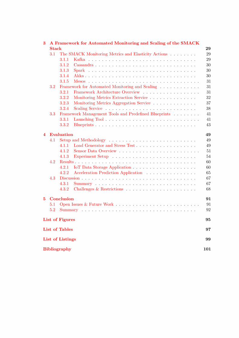
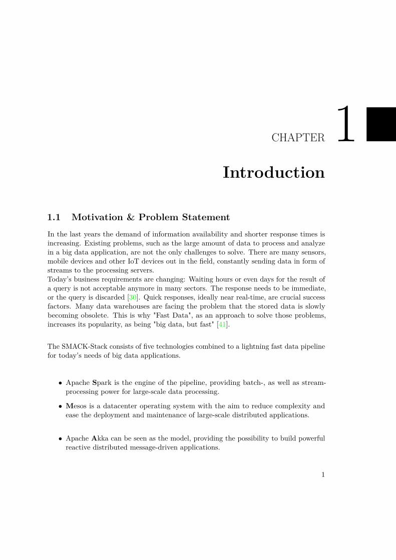
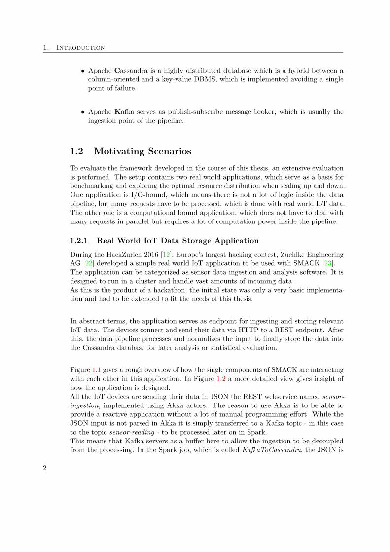
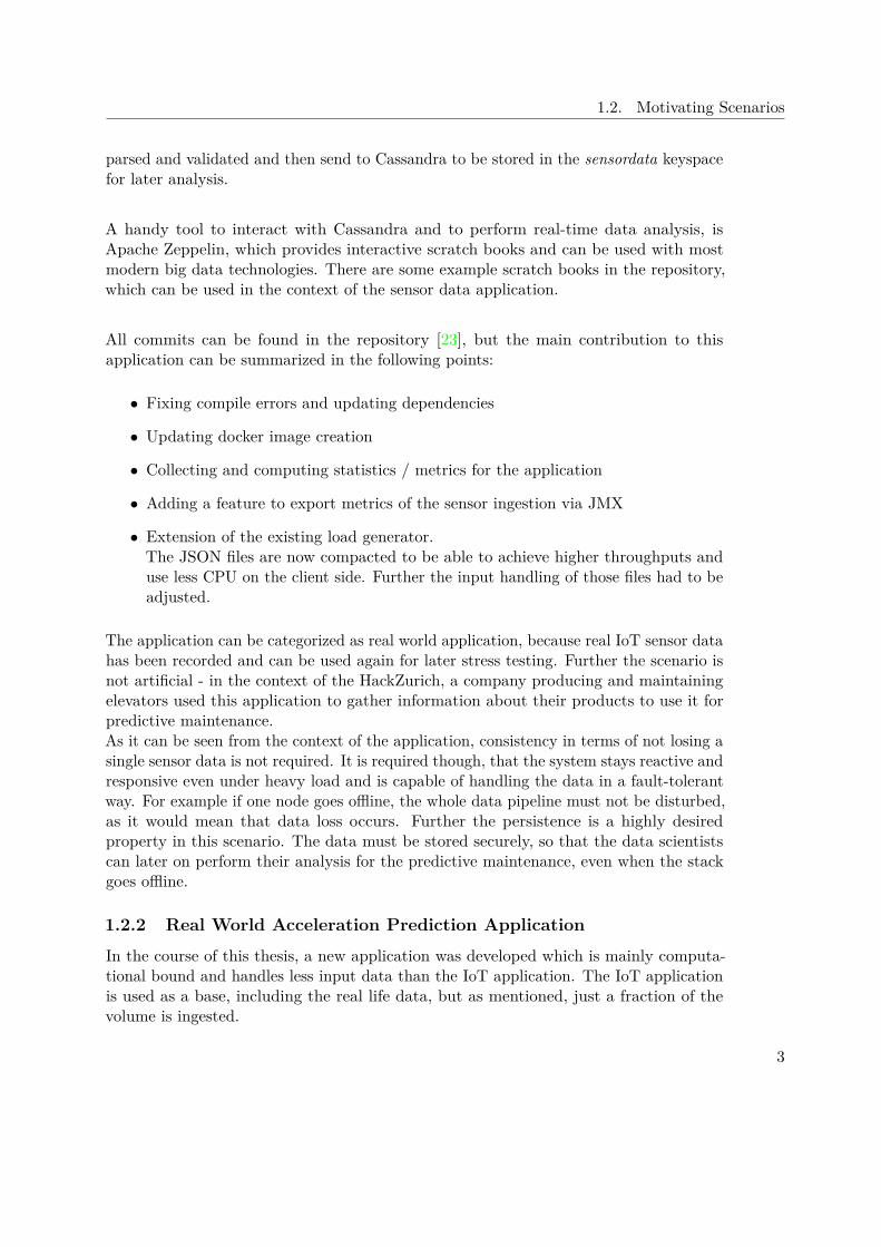
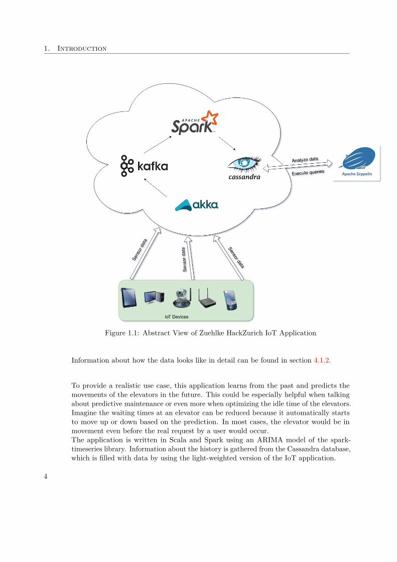
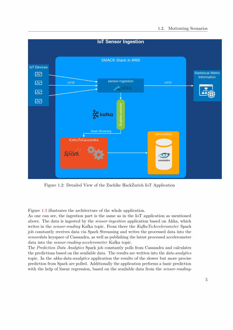
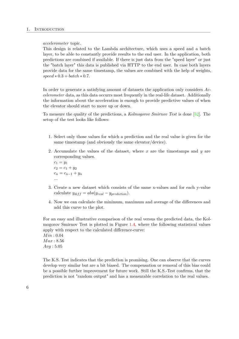
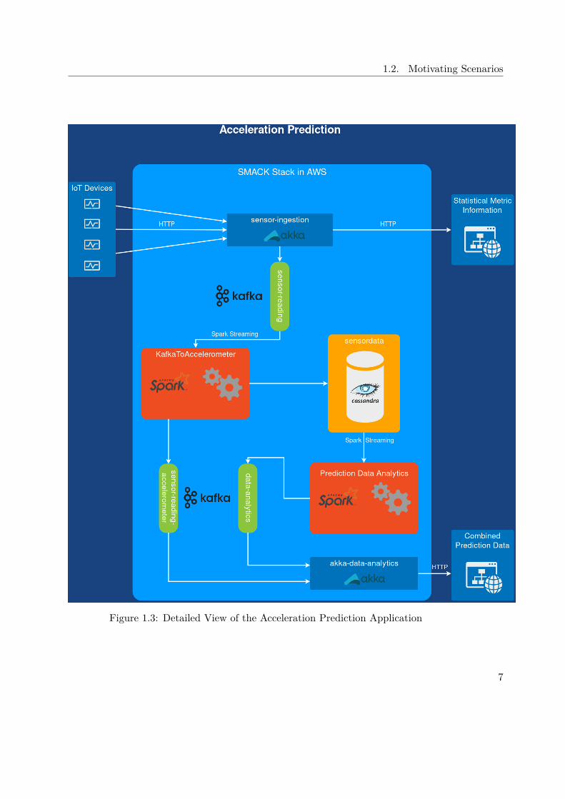
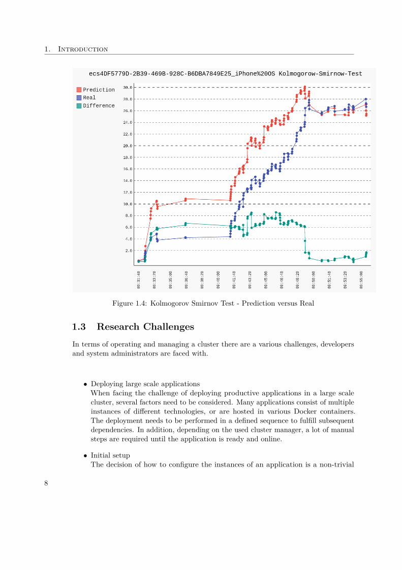
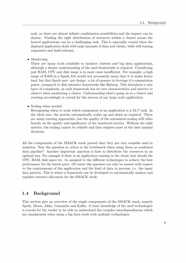
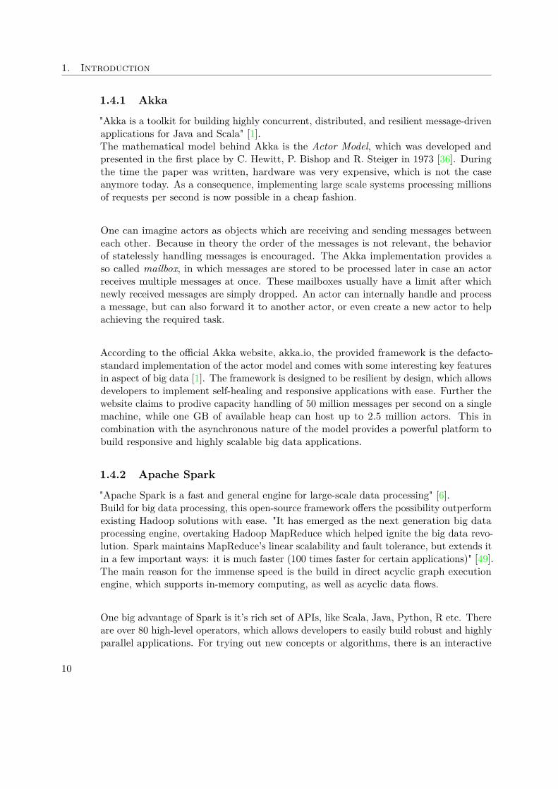
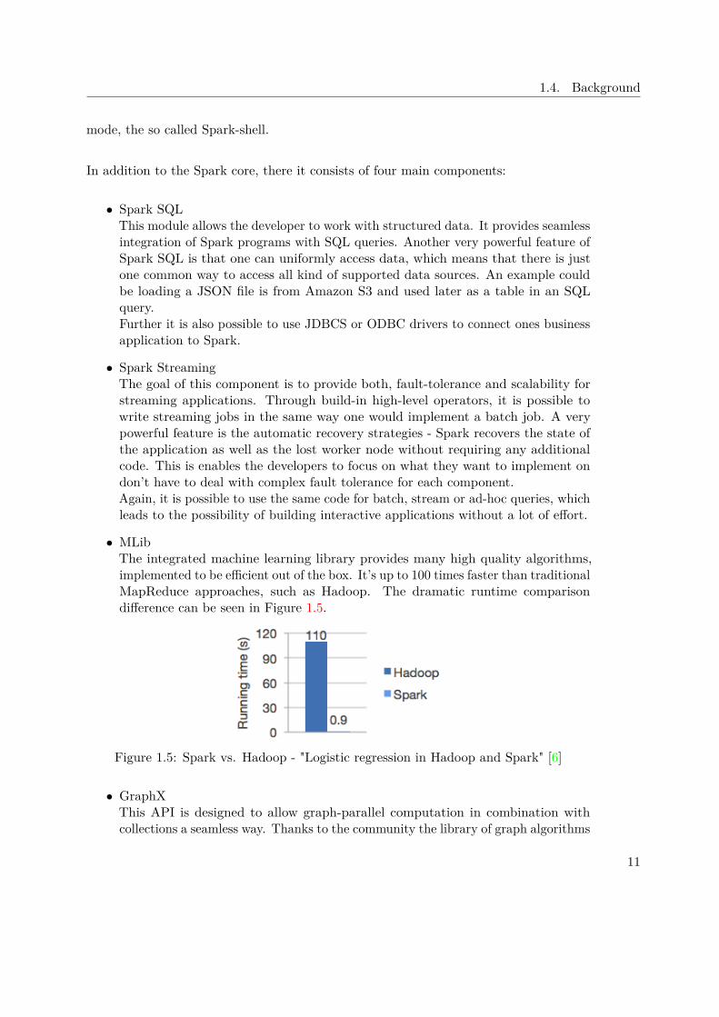
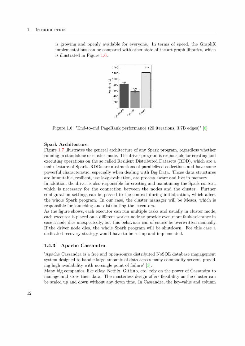
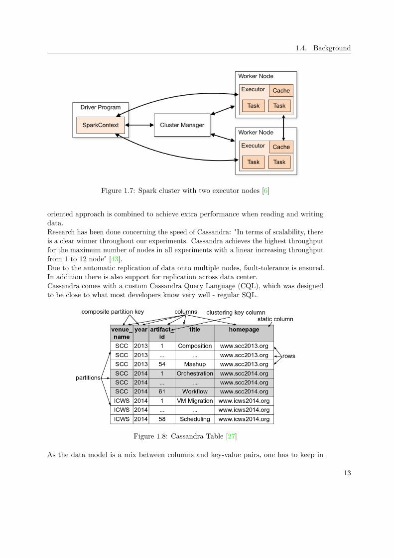
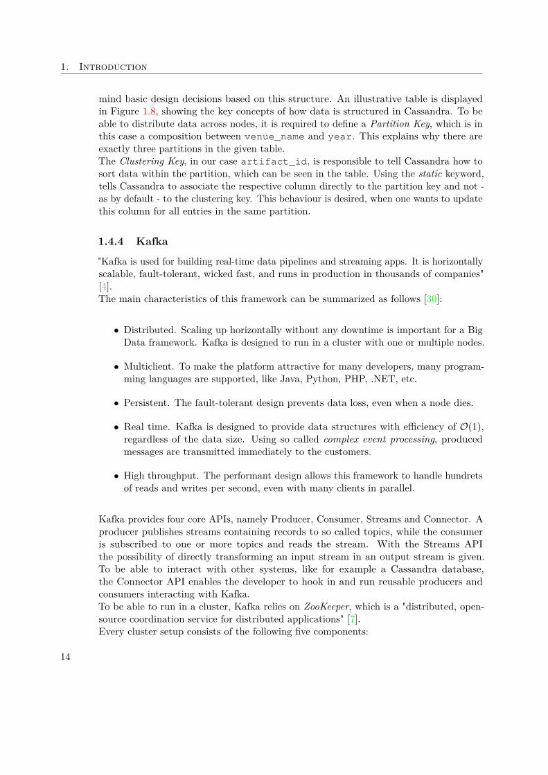
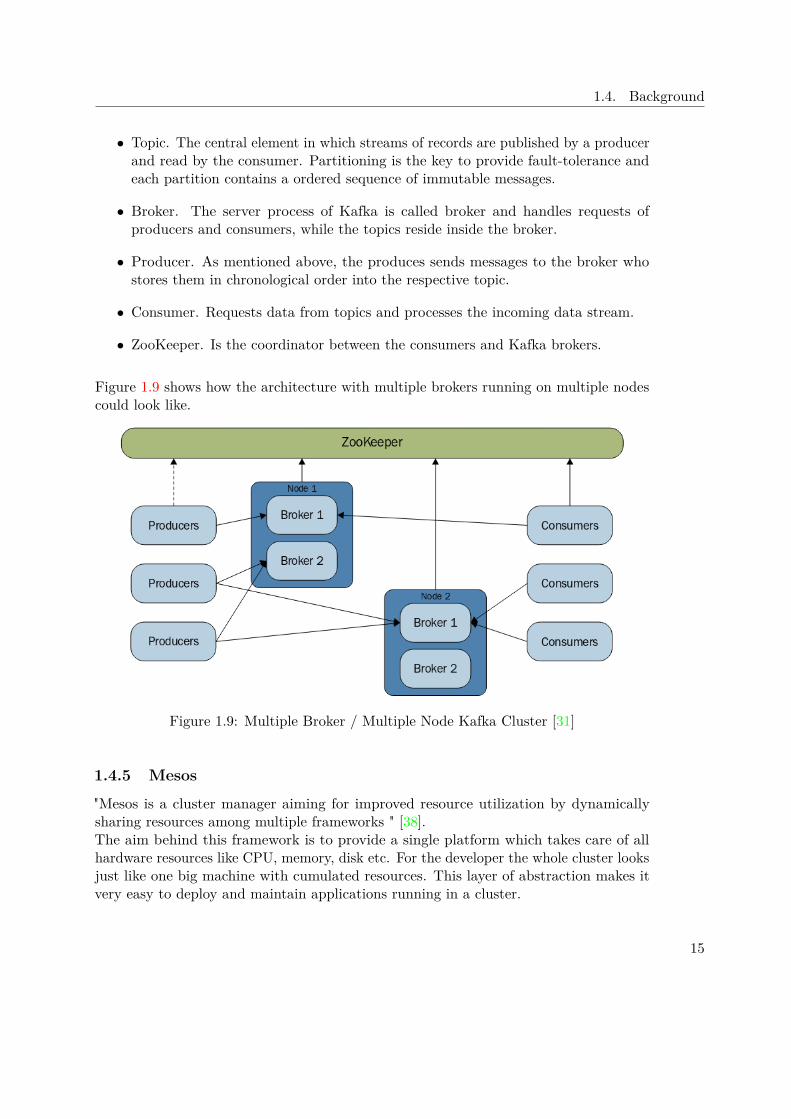

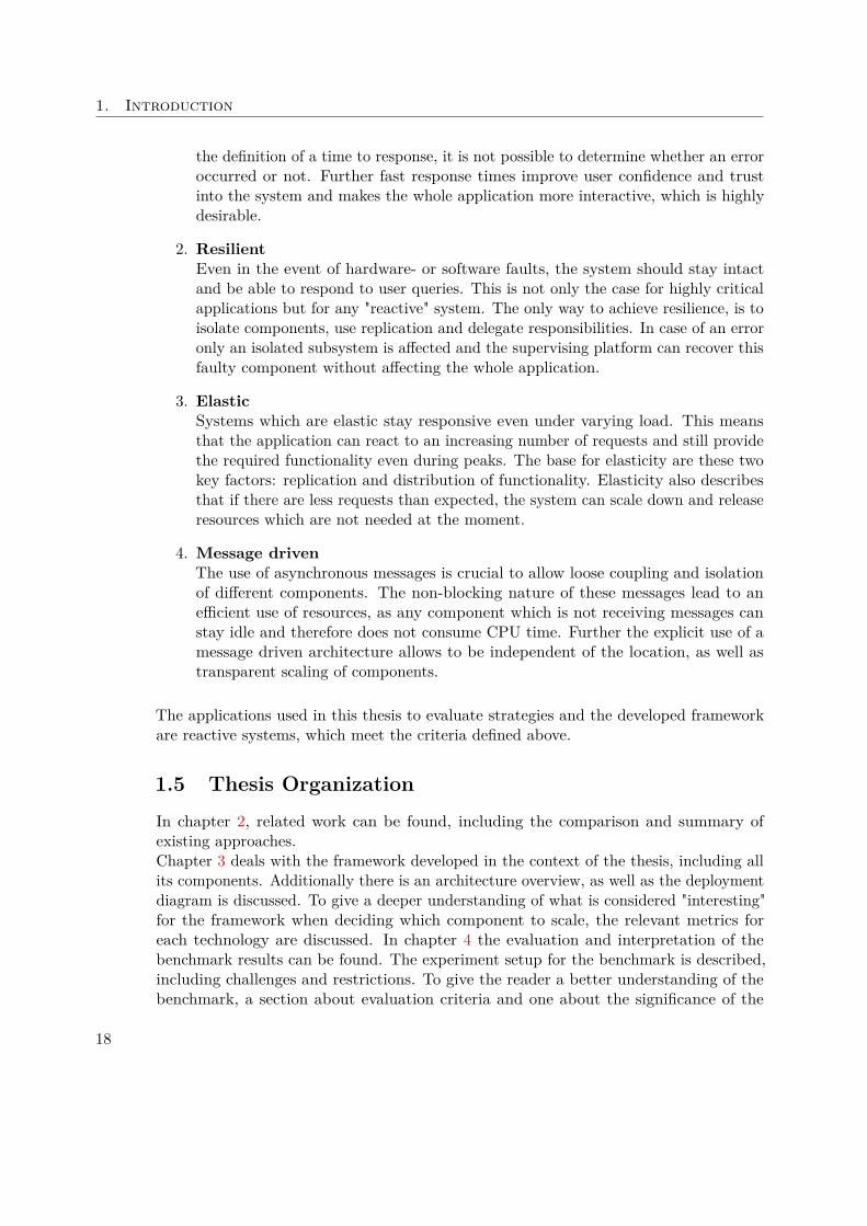
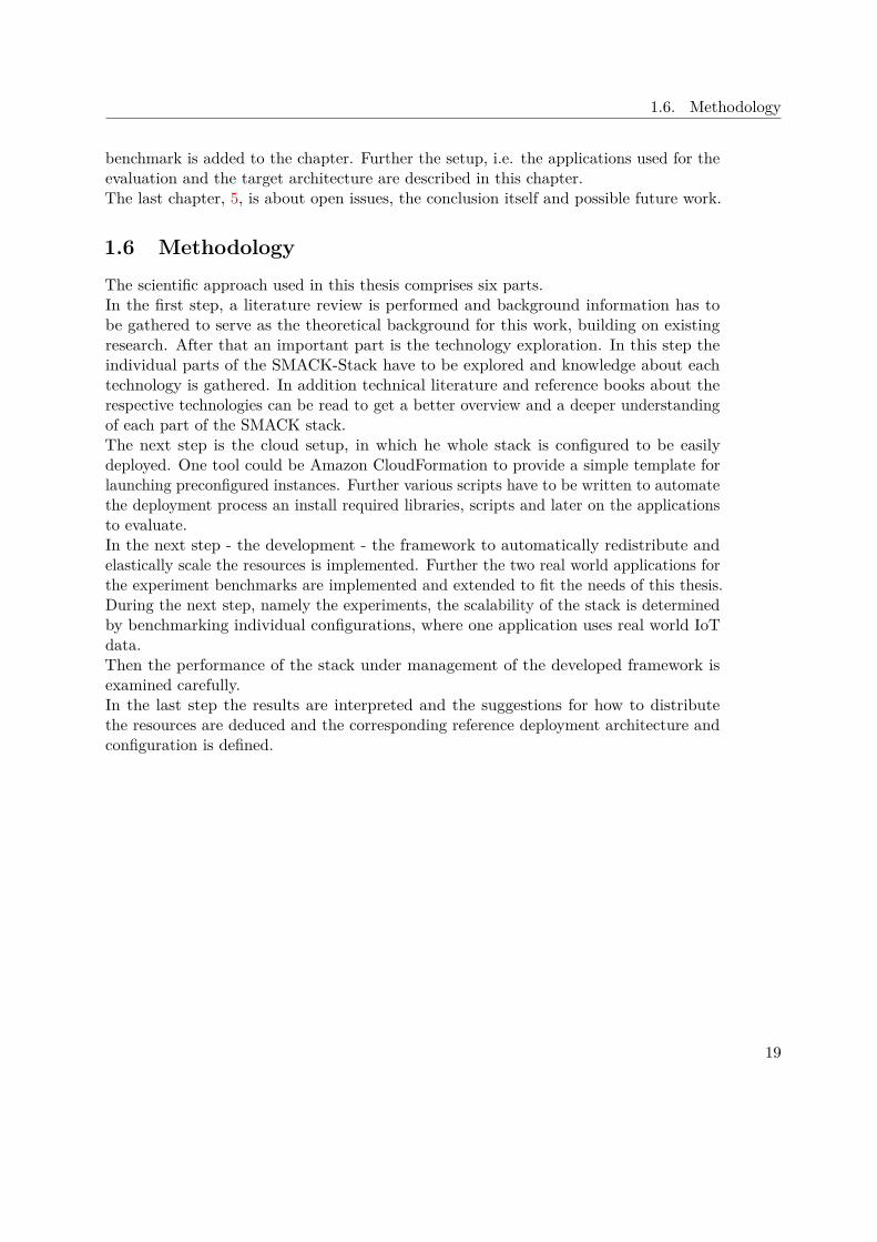

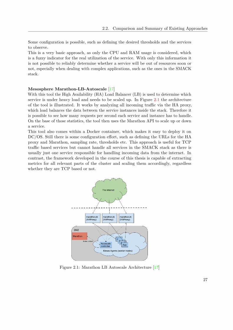
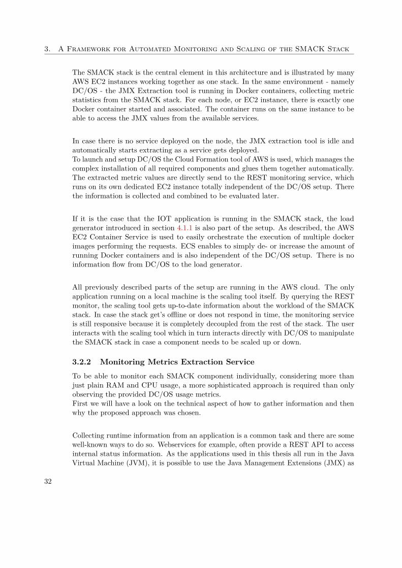
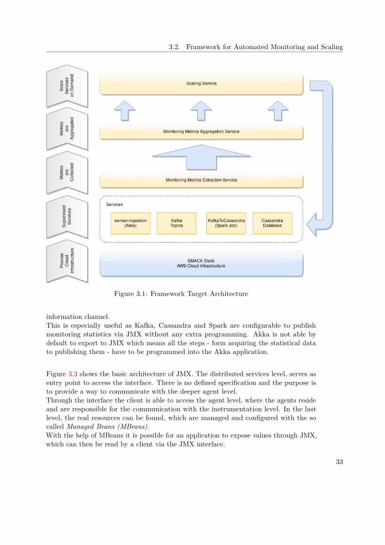
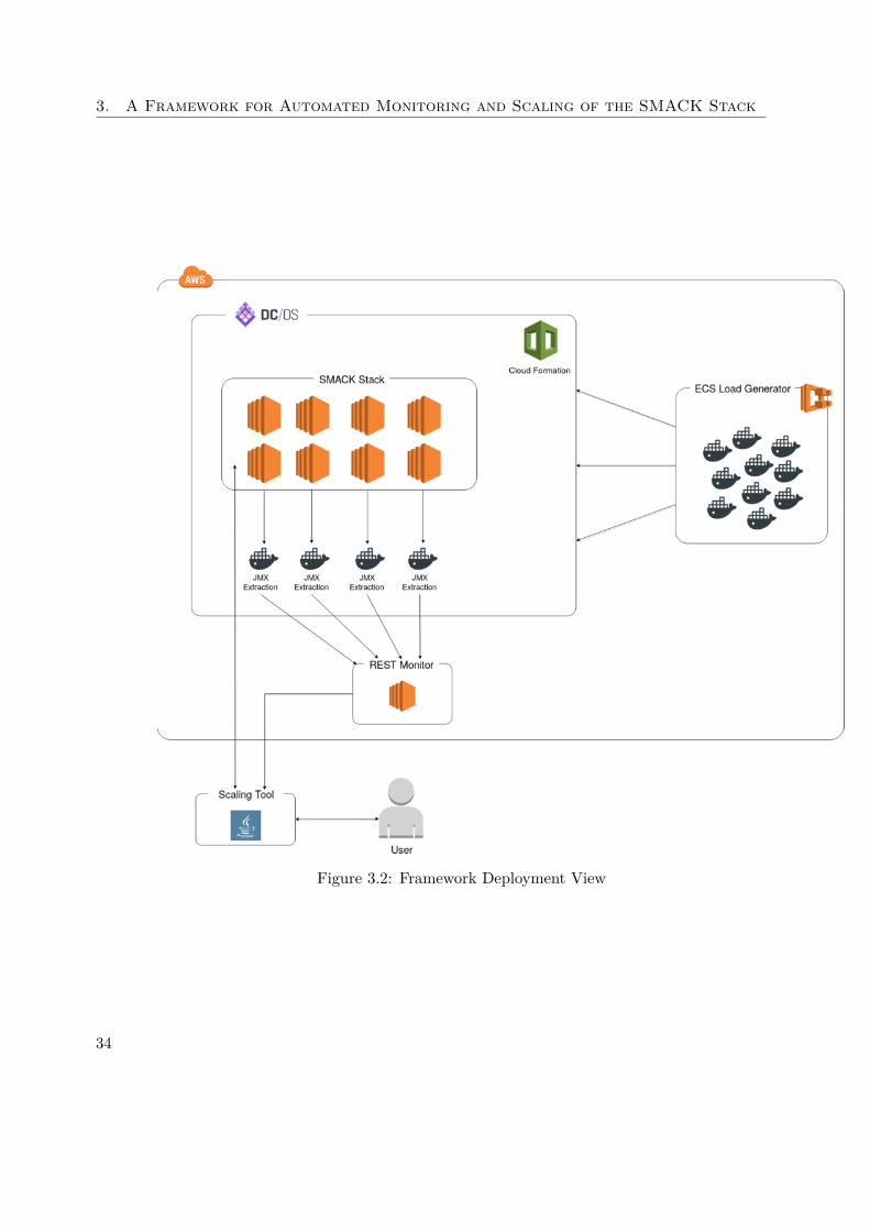
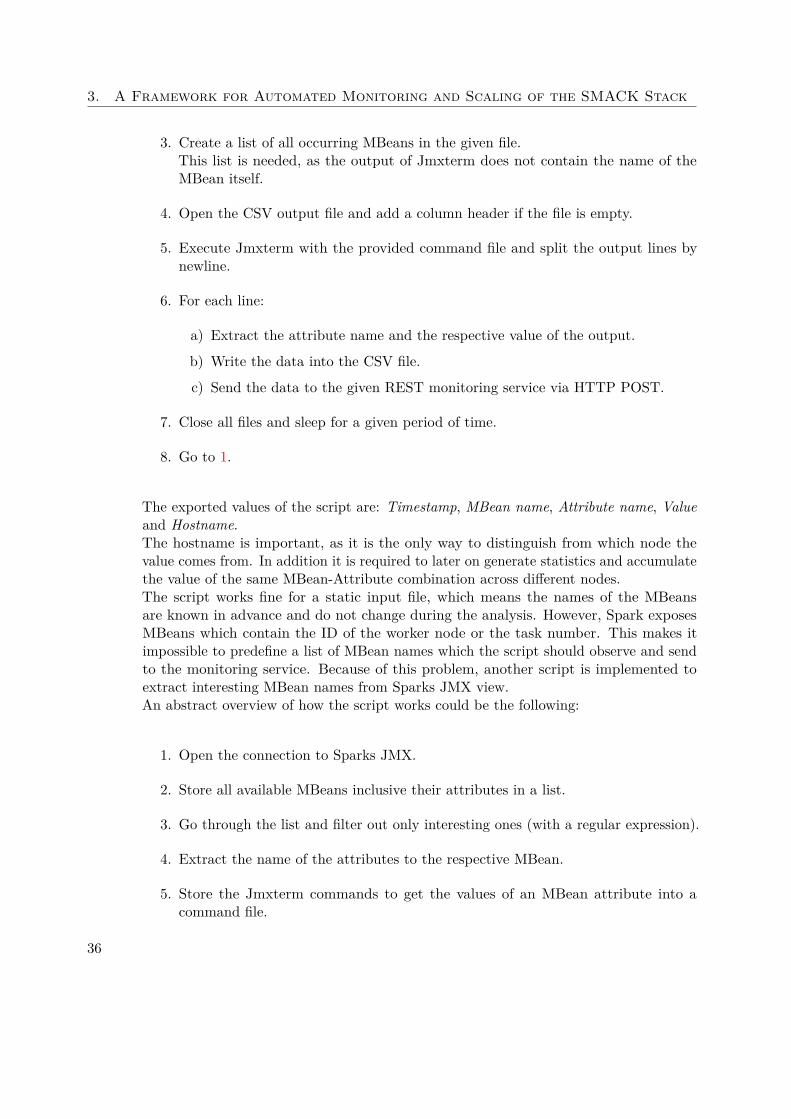
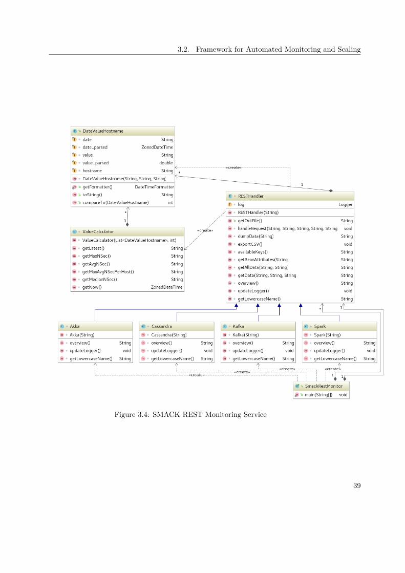
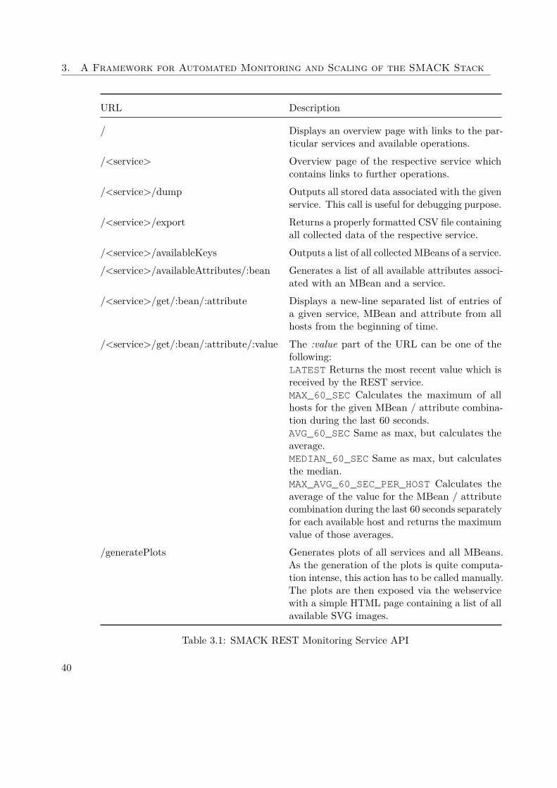
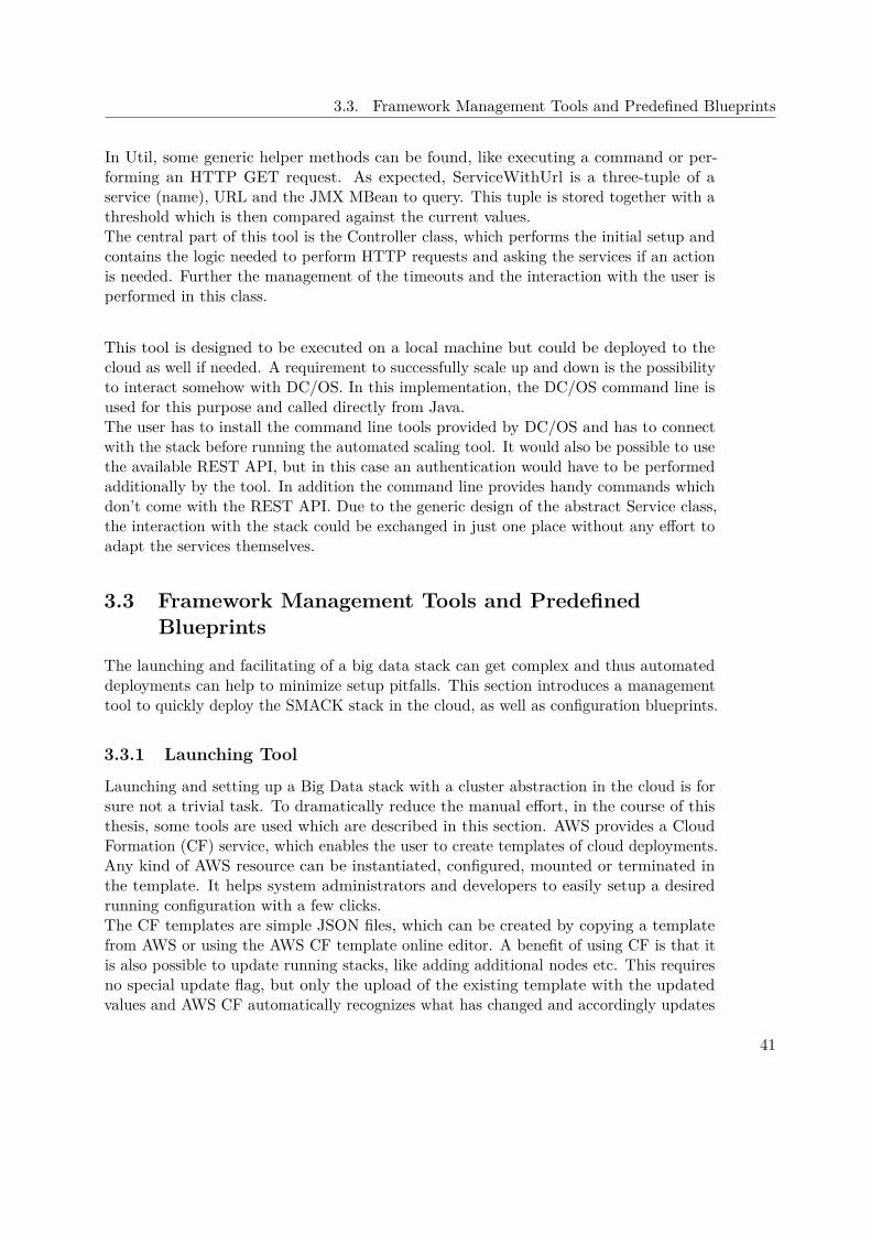
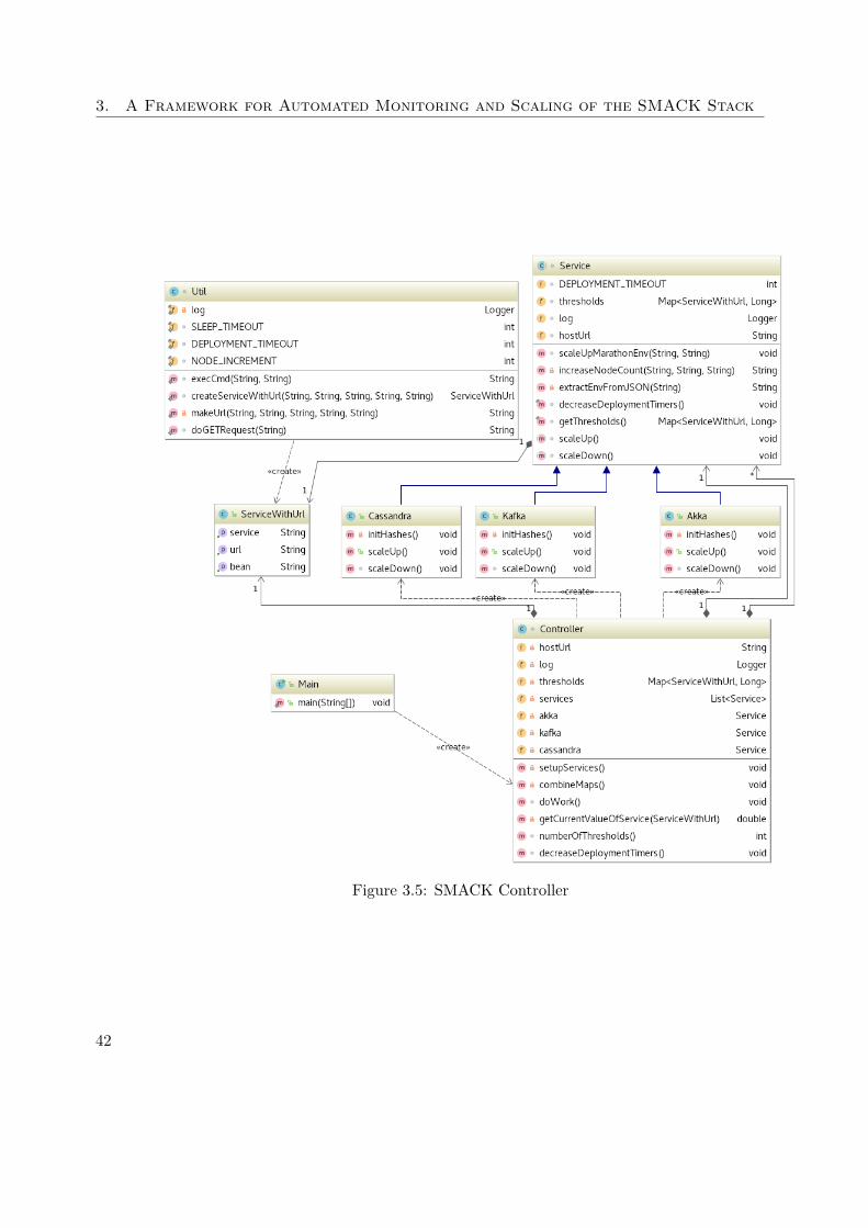
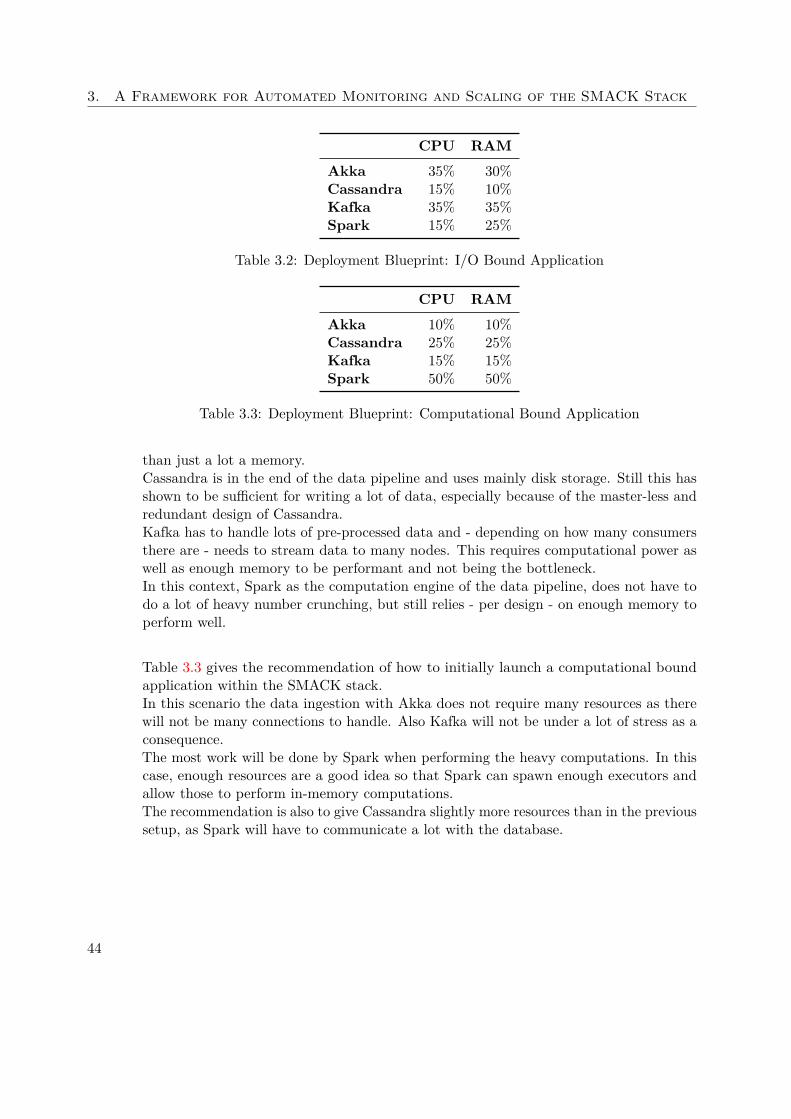
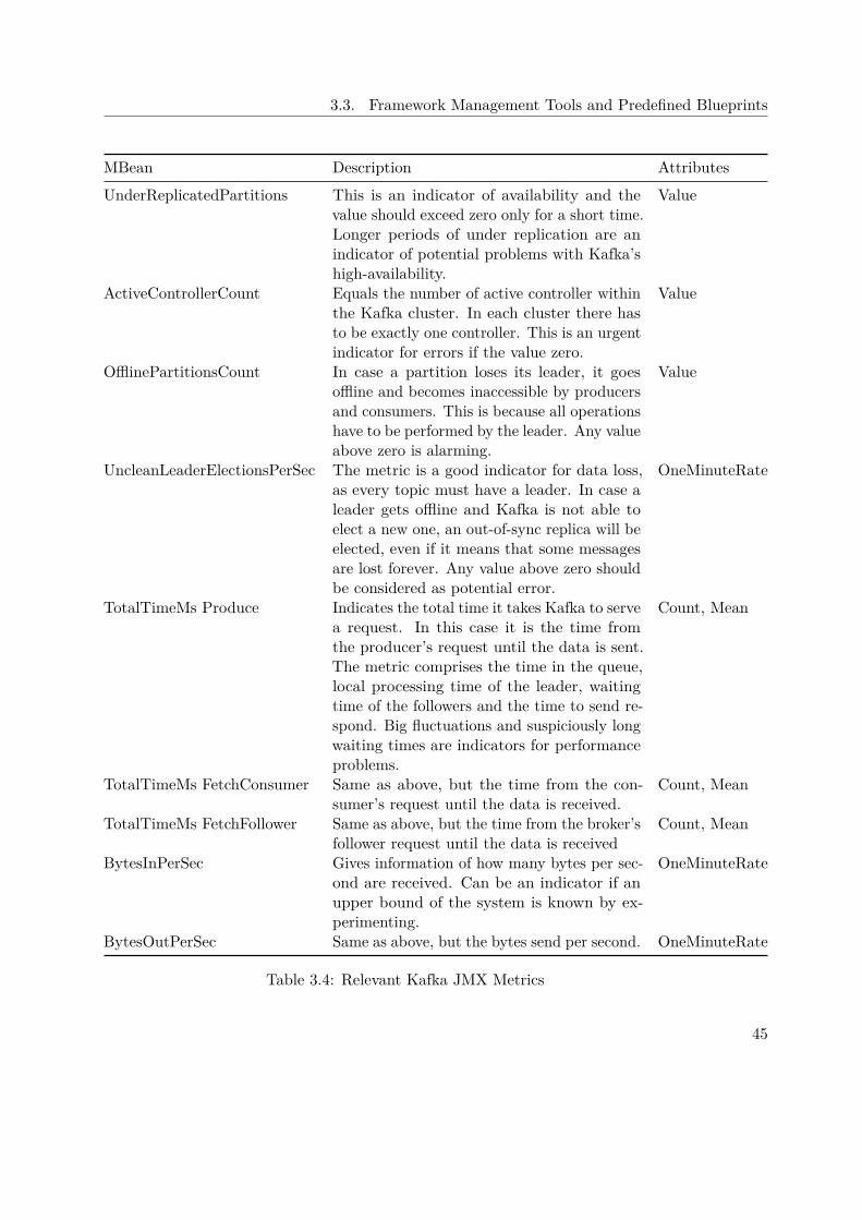

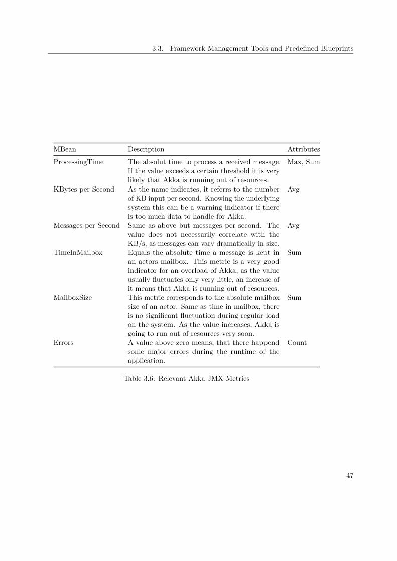
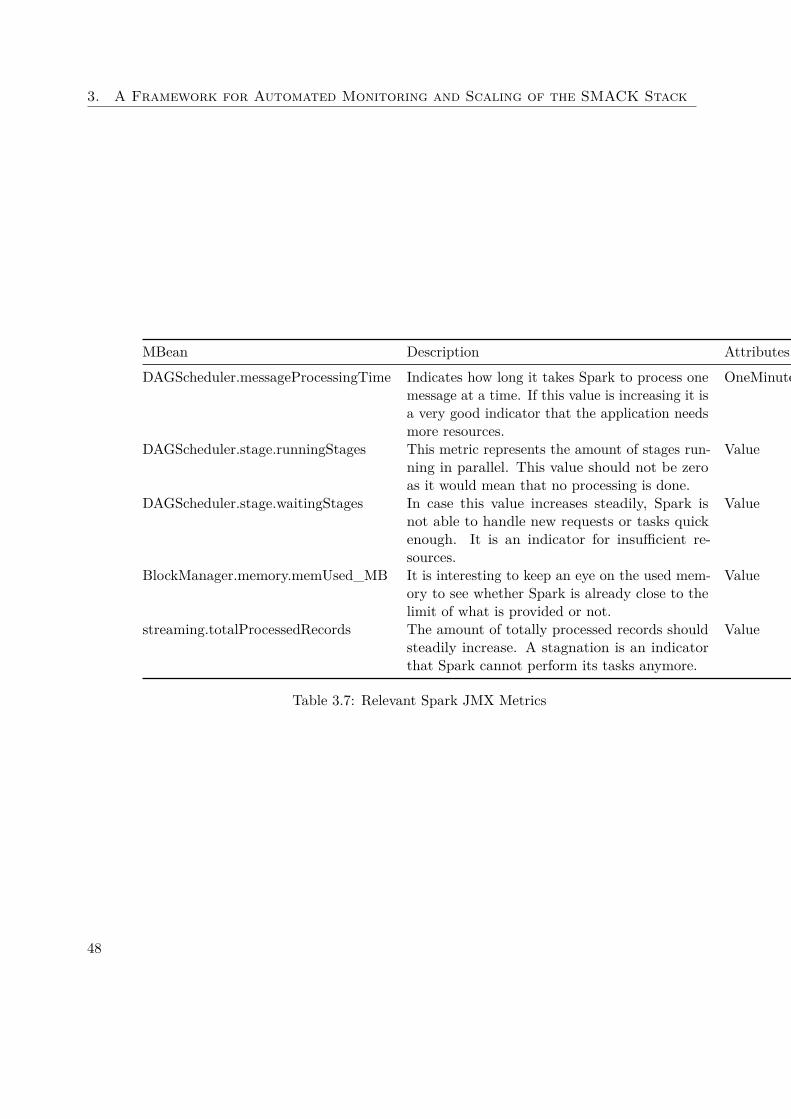
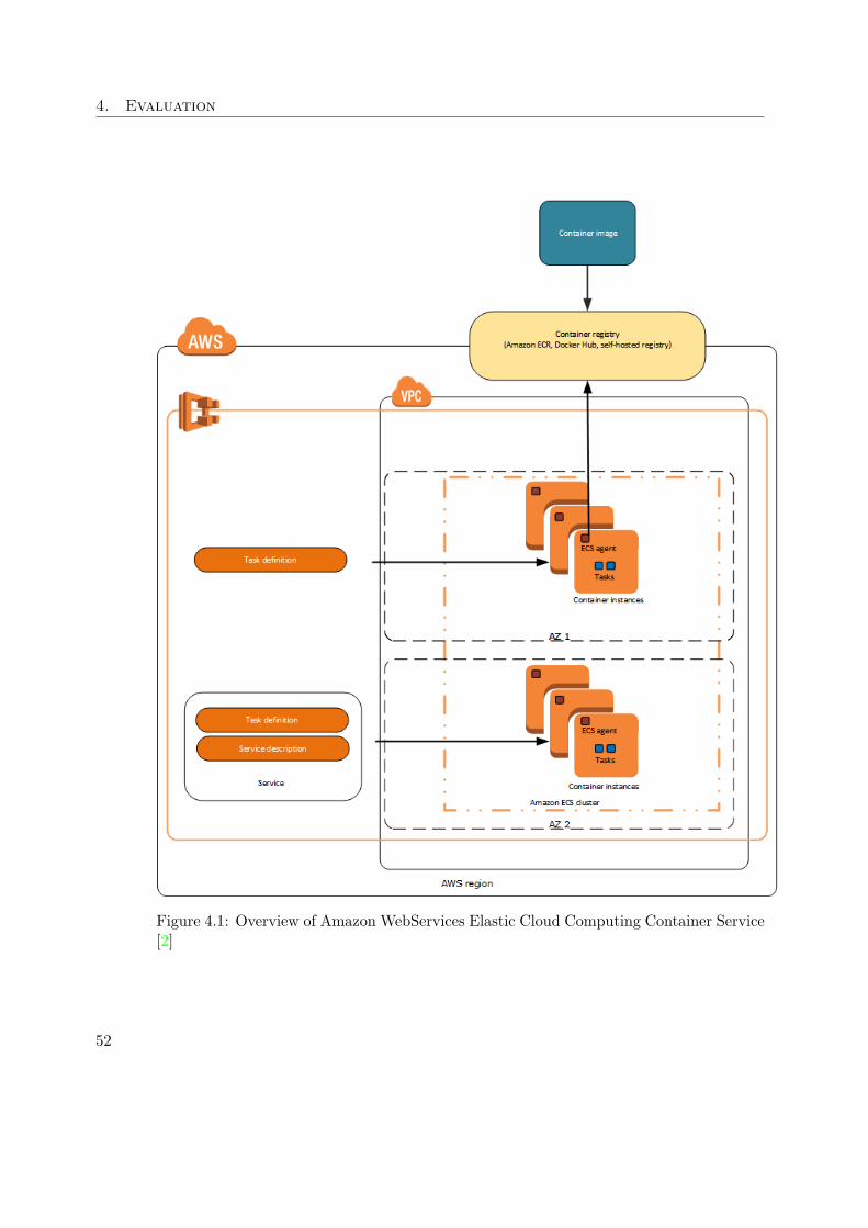
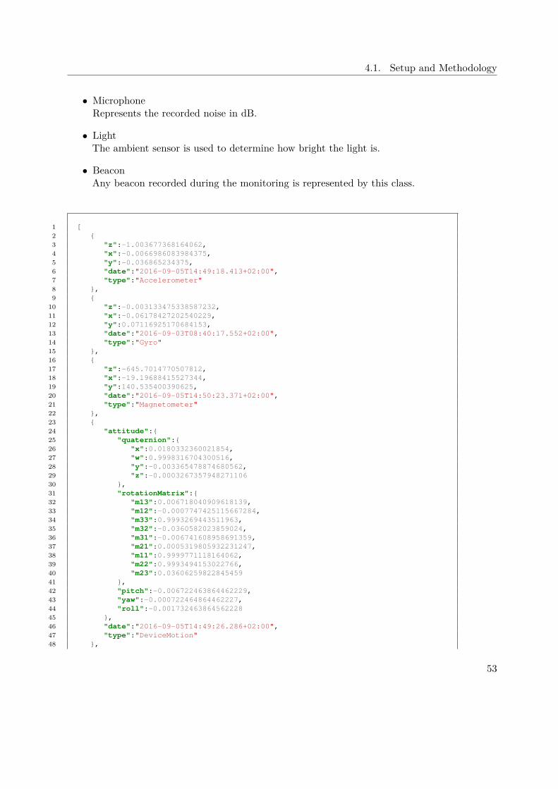
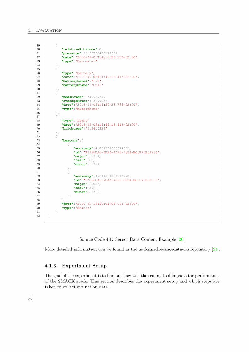
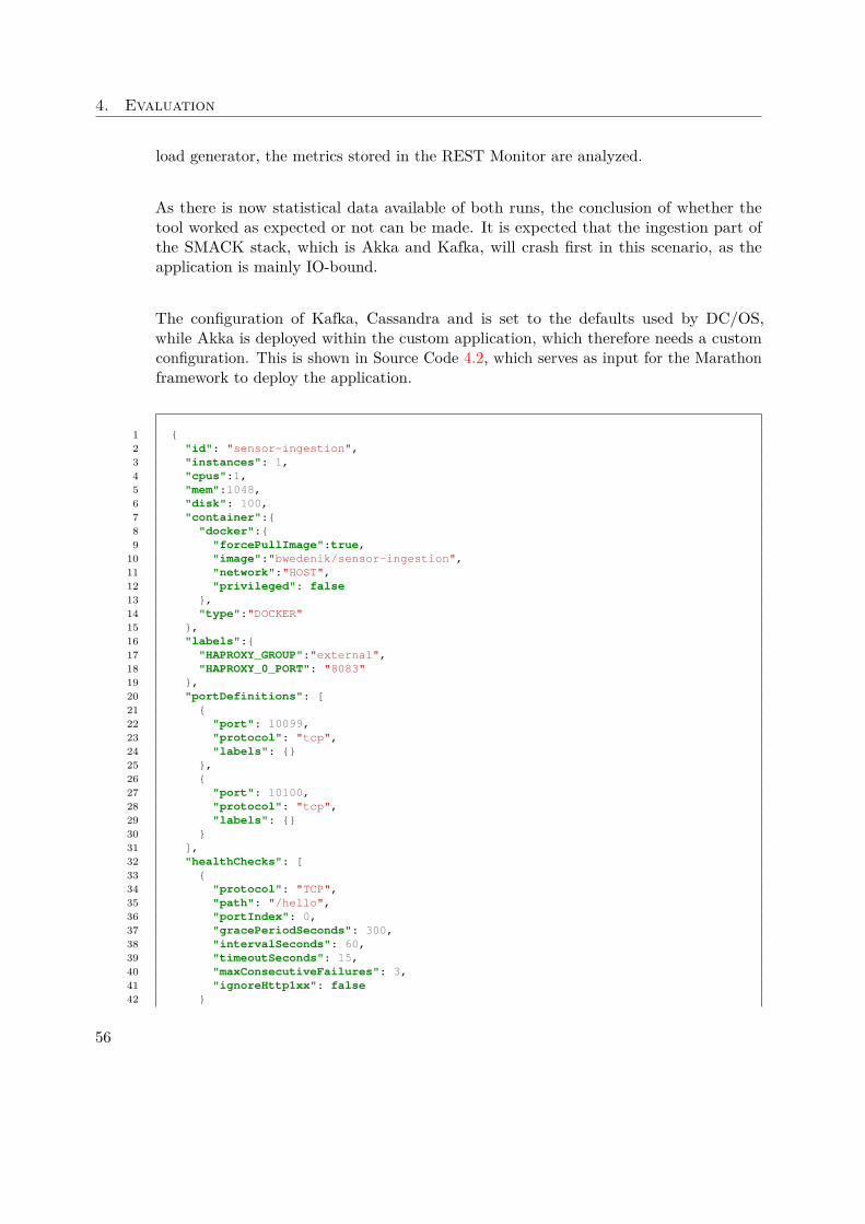
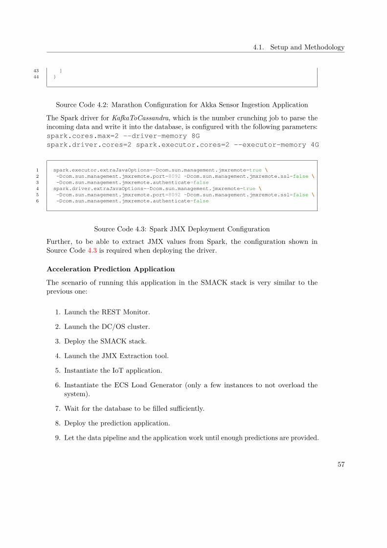
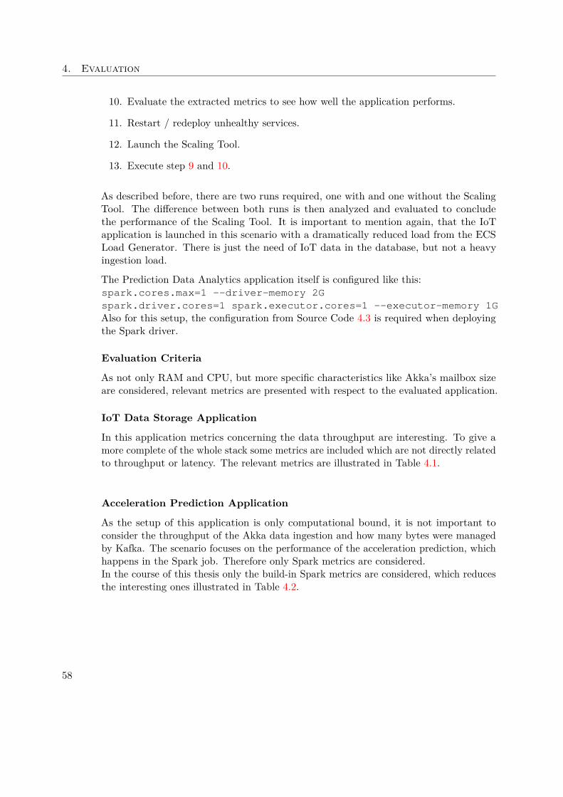
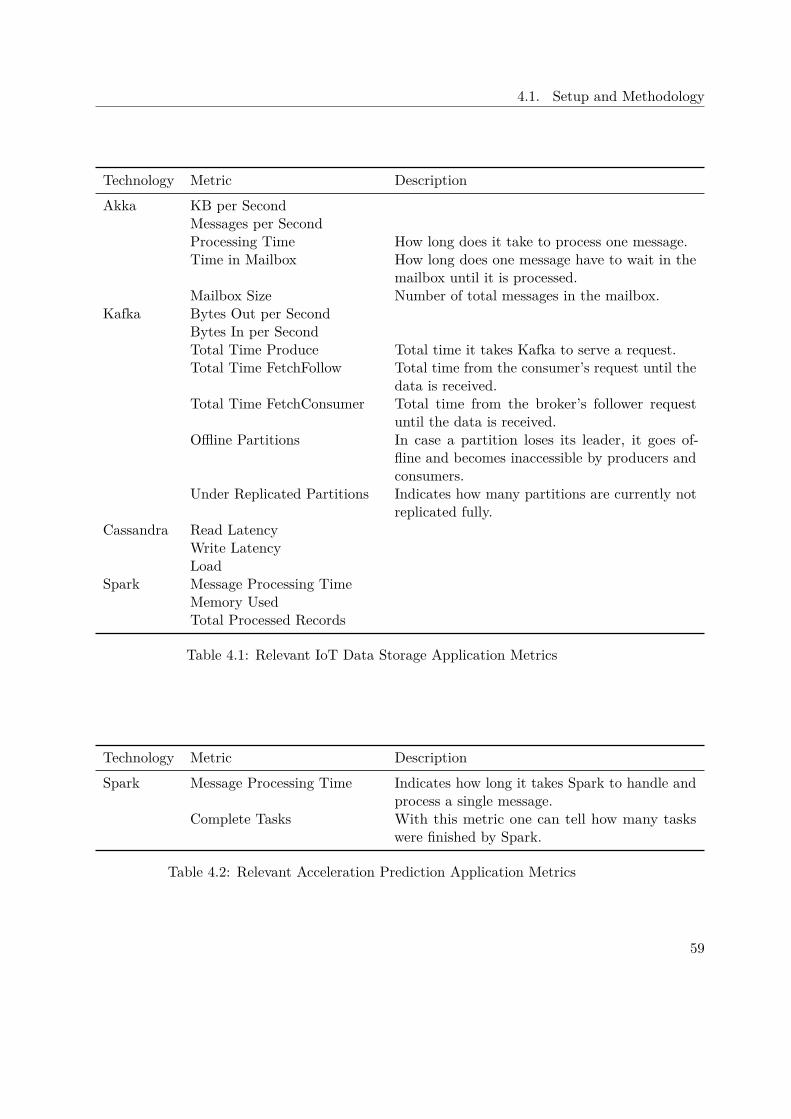
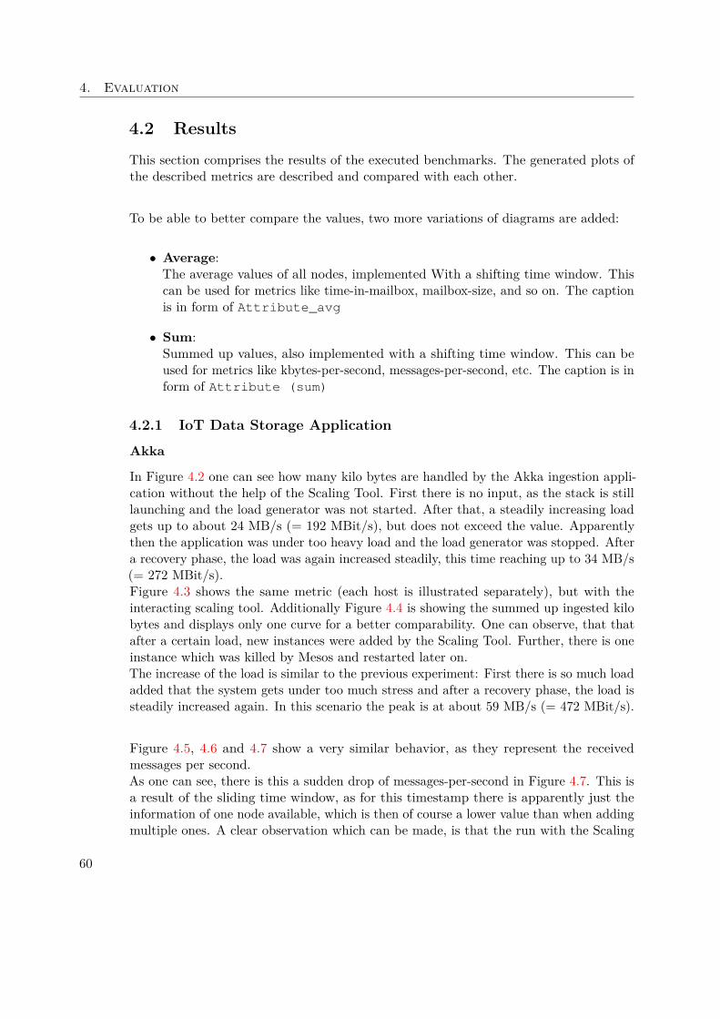
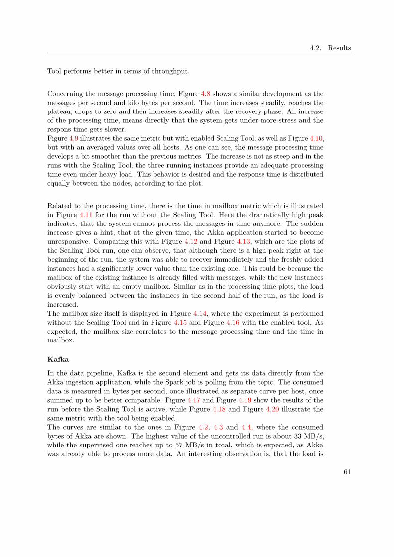
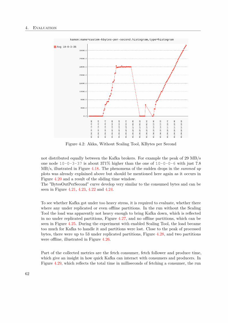
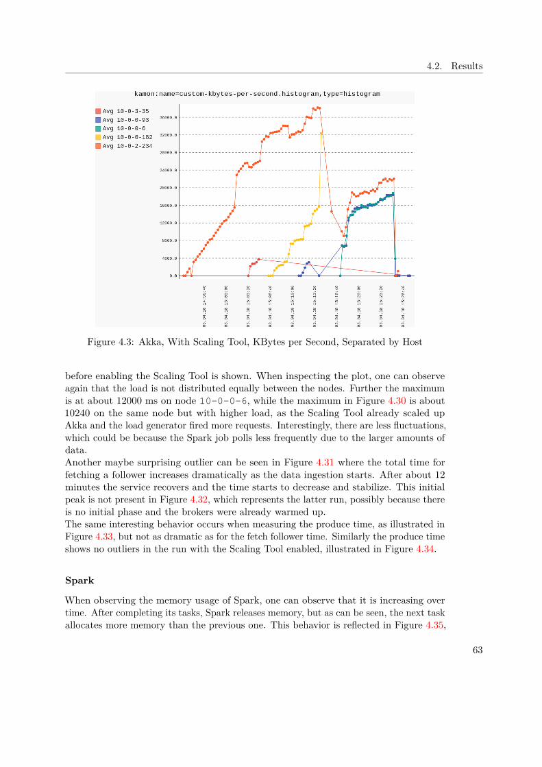
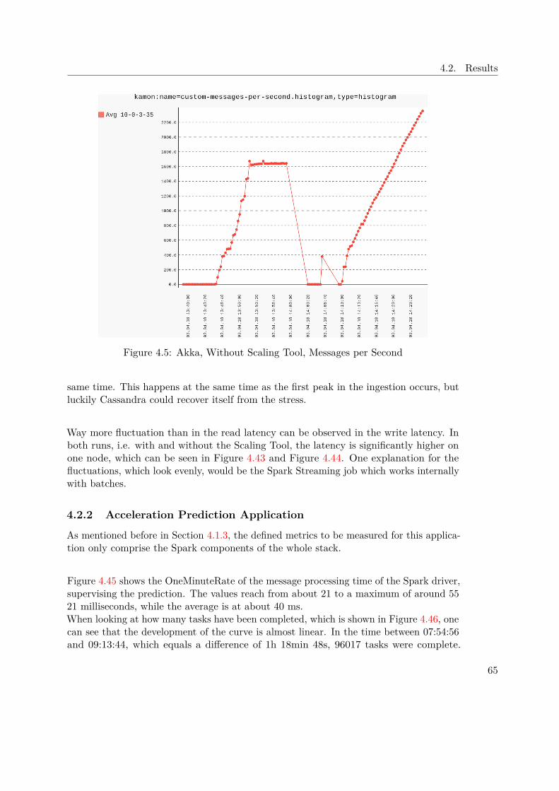
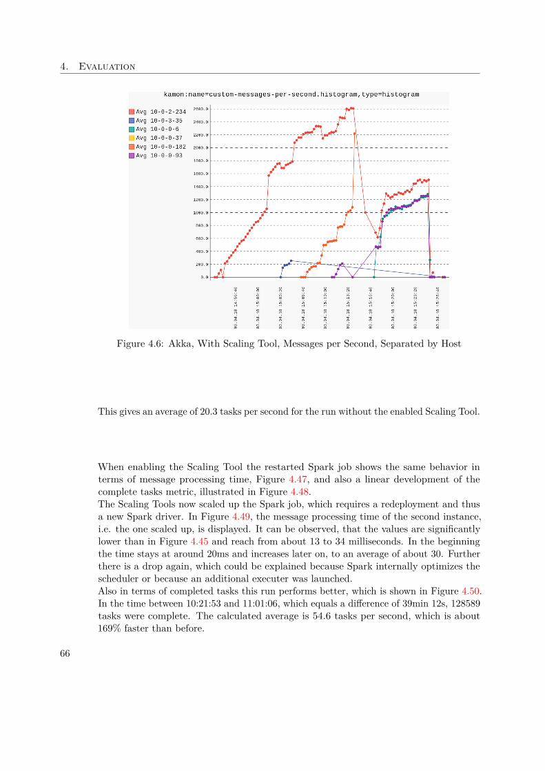
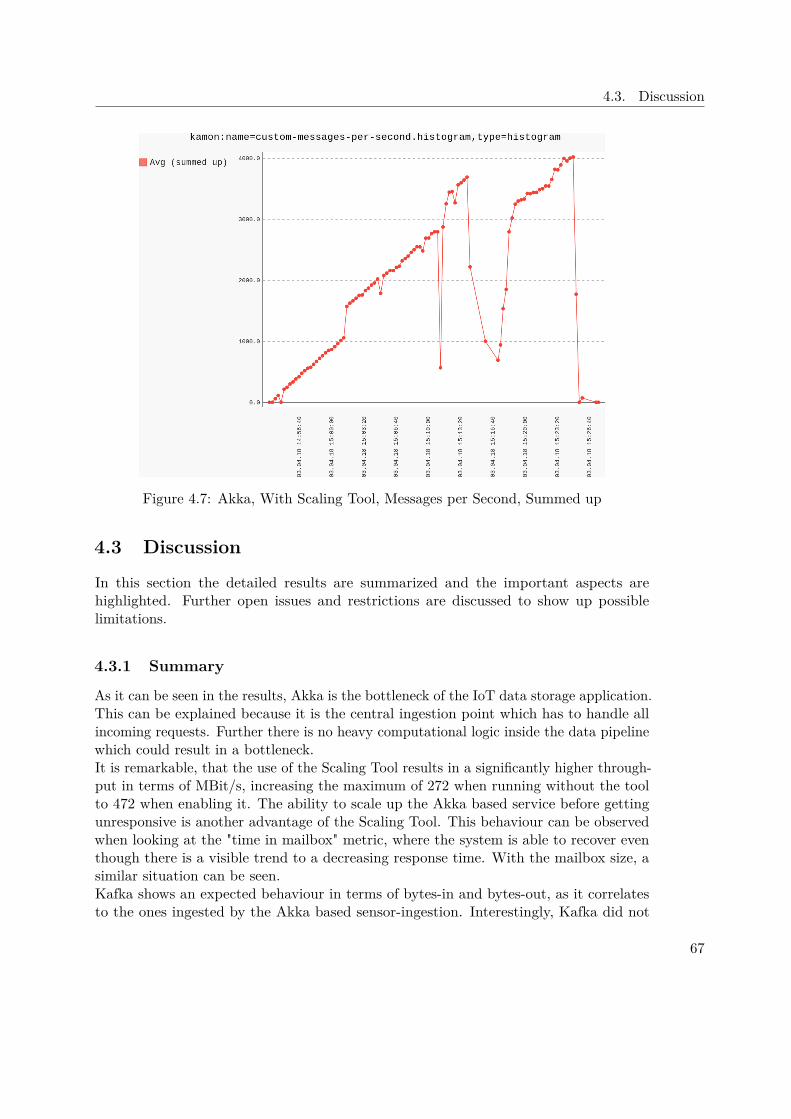
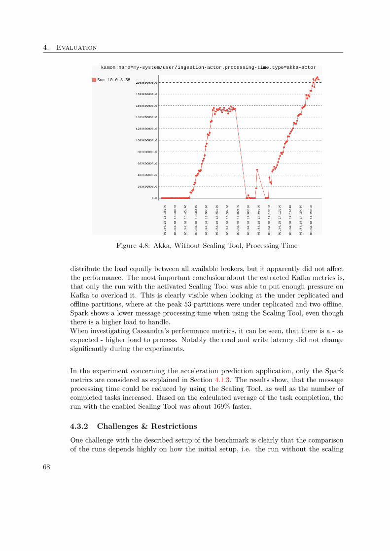
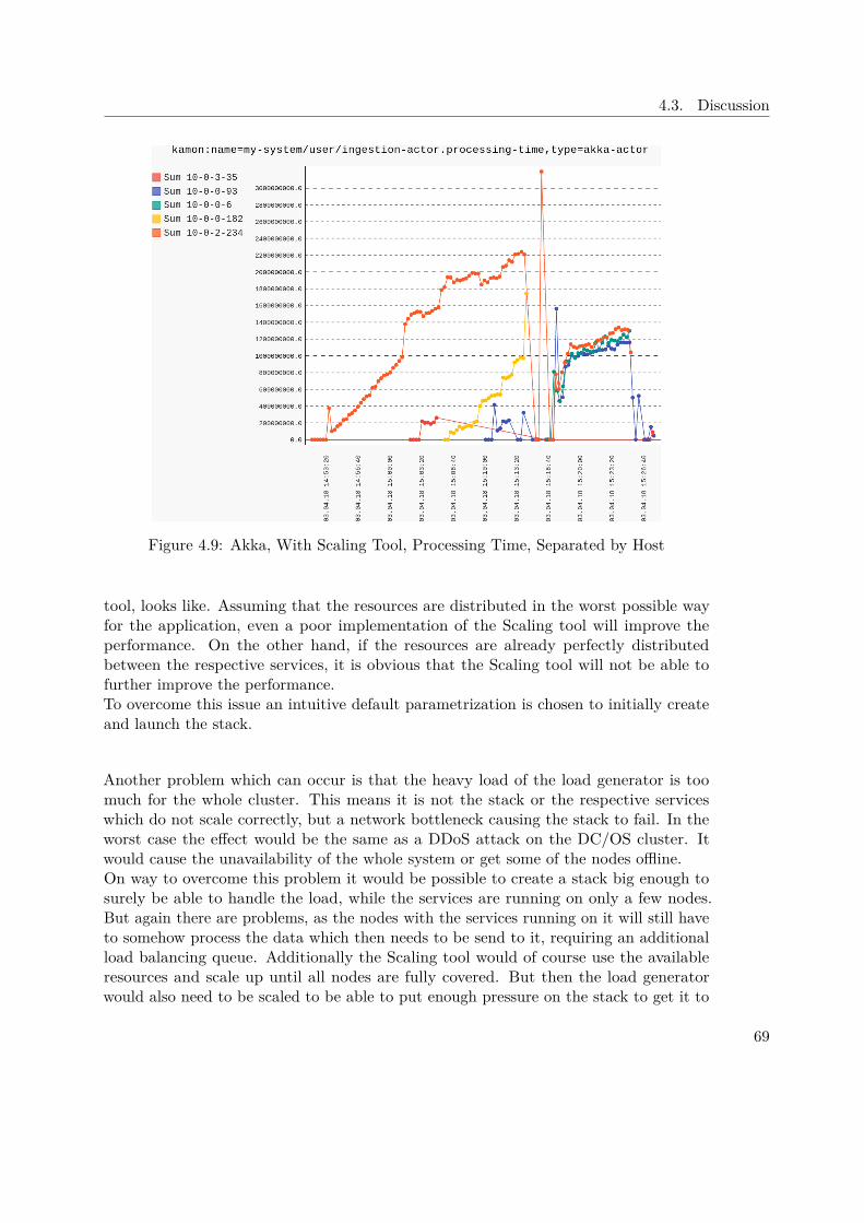
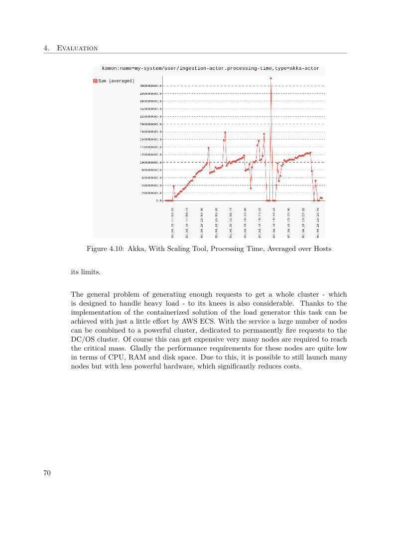
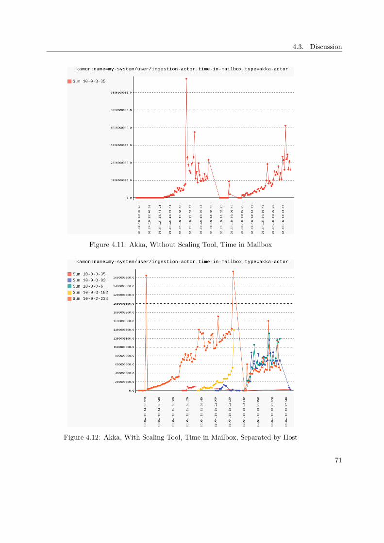
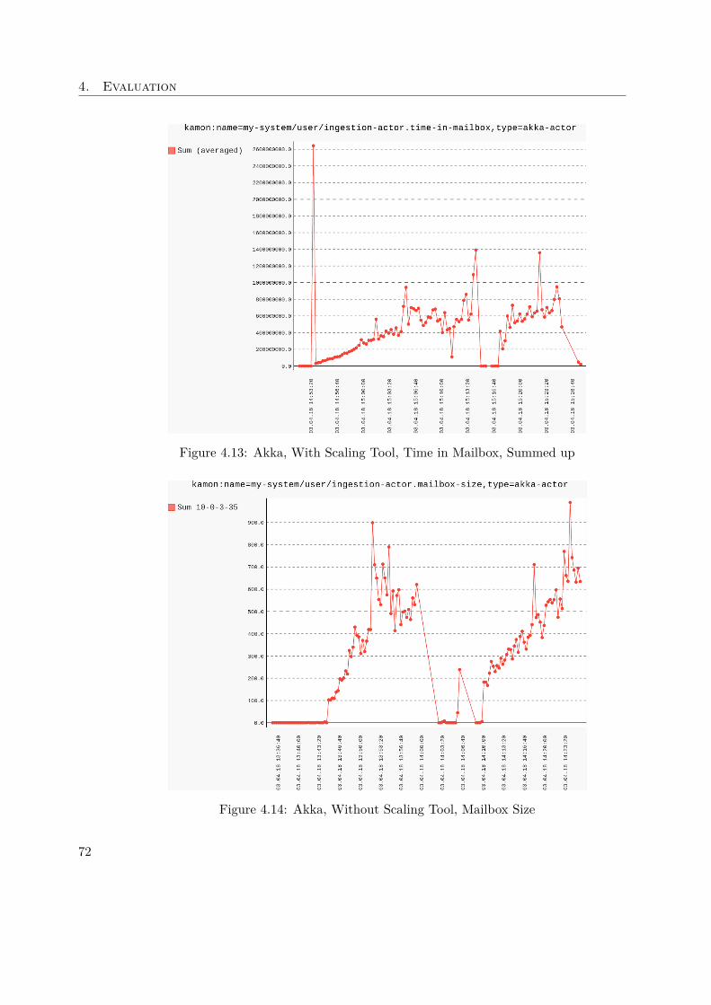
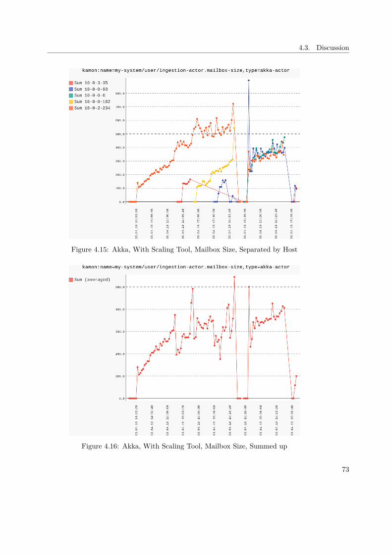
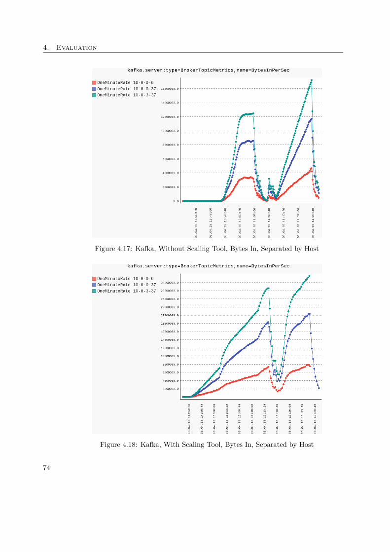
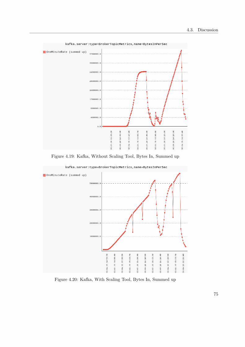
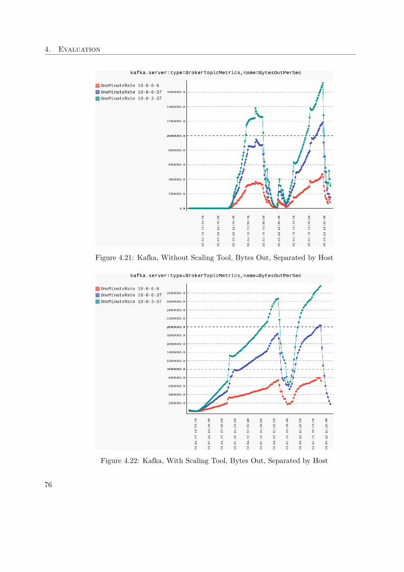
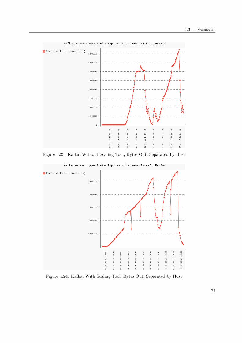
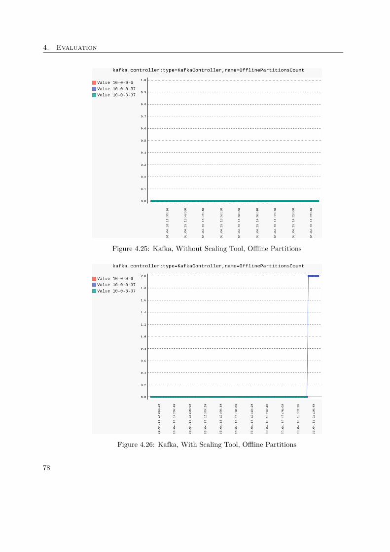
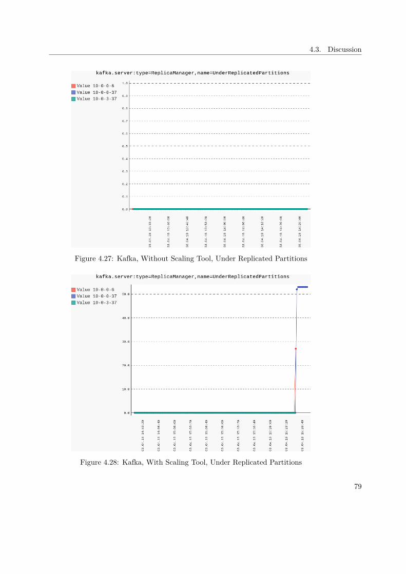
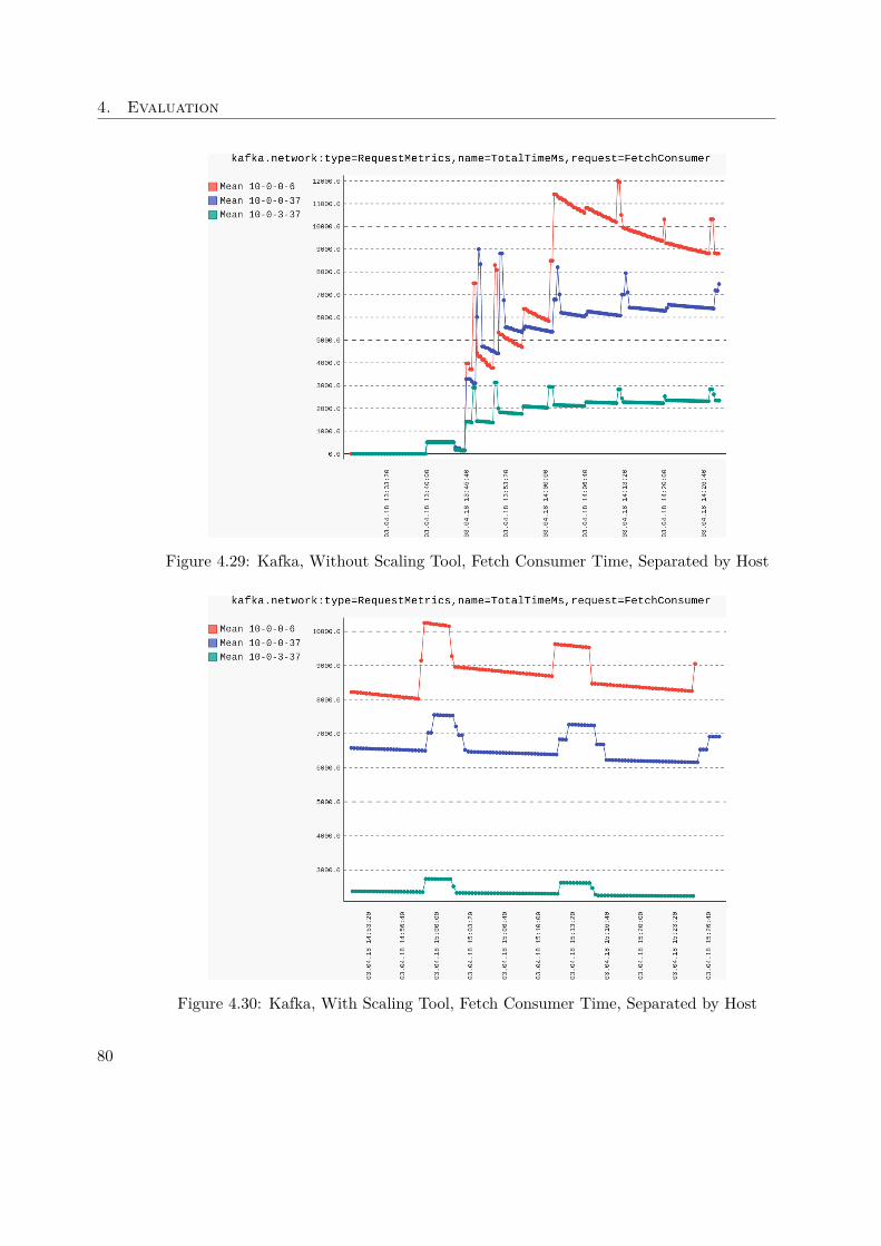
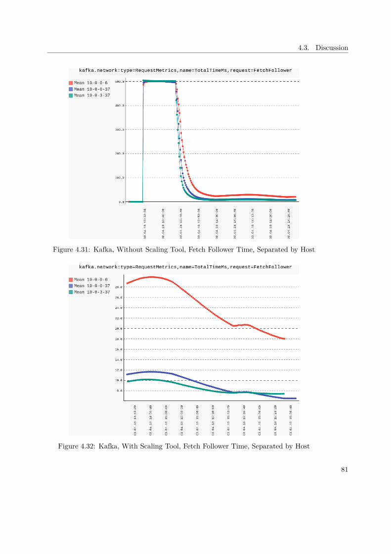
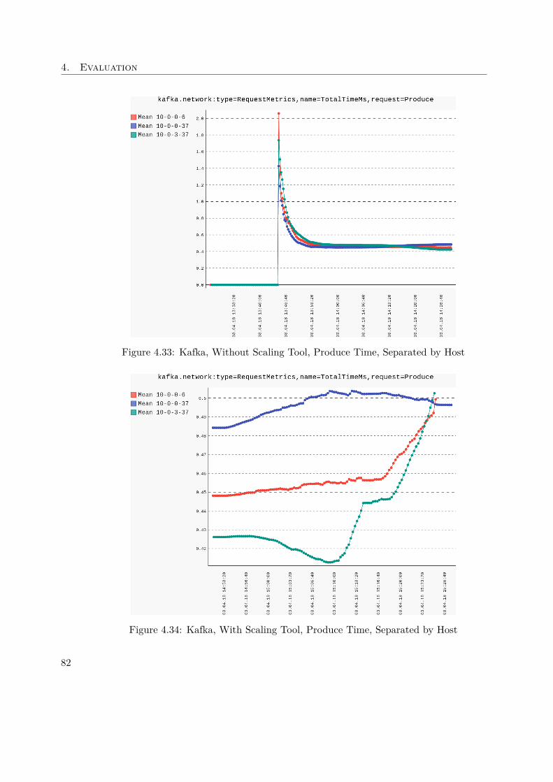
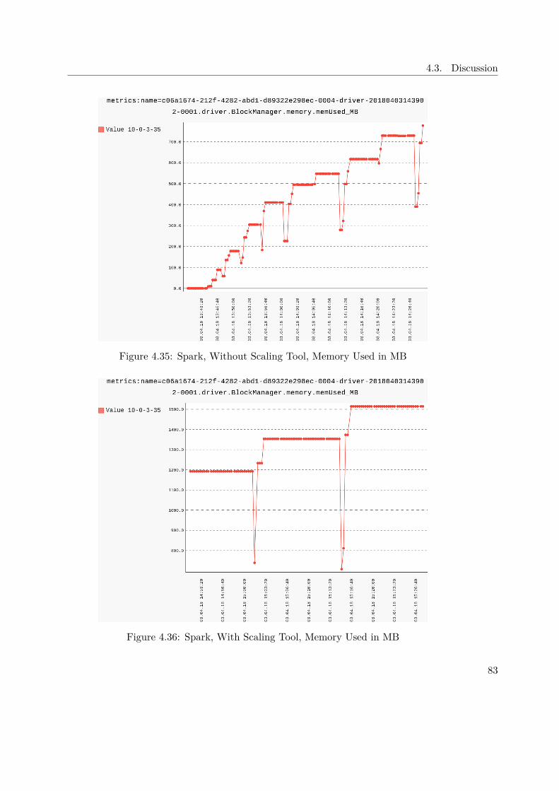
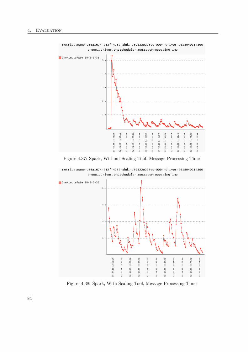
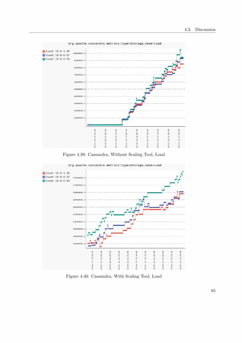
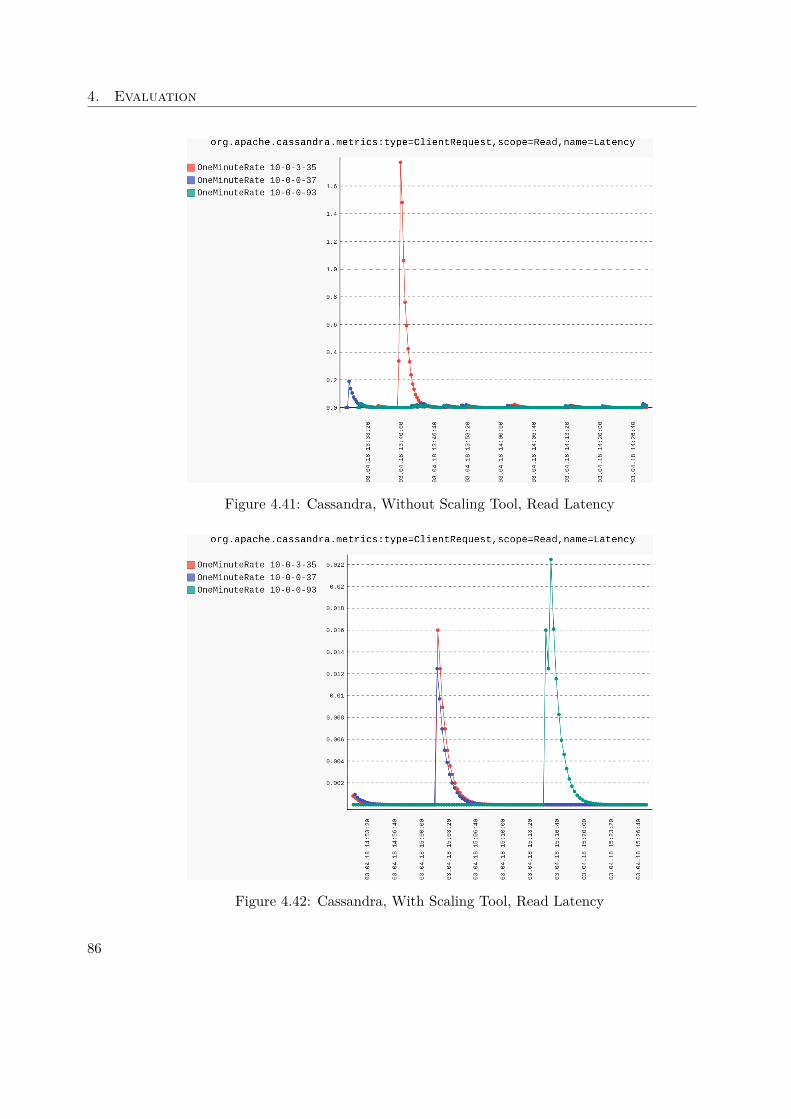
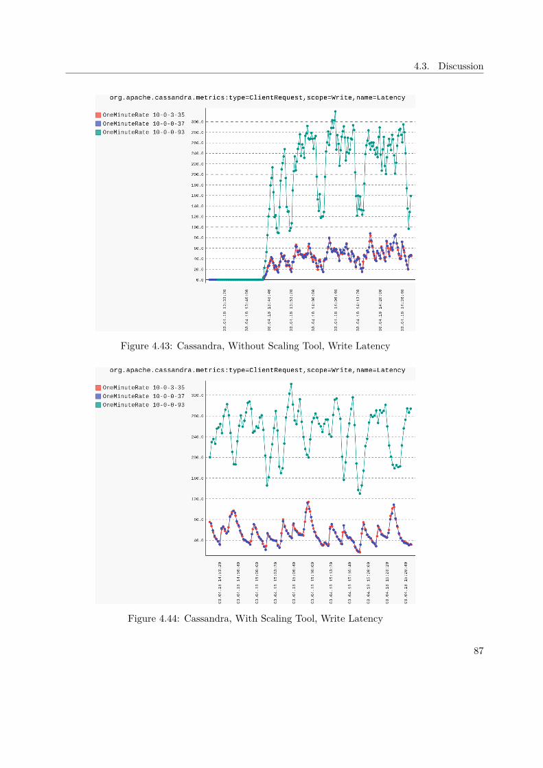
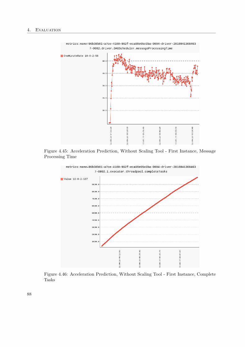
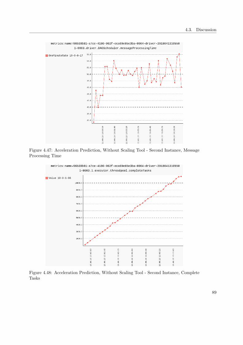
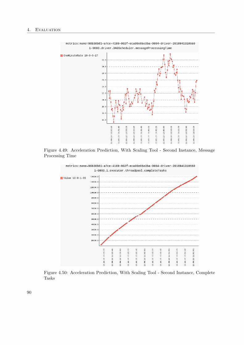
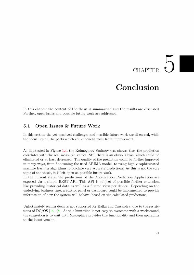
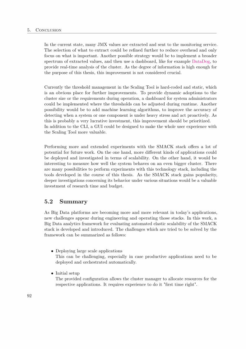


![Evaluating Life Expectancy Estimates › fileadmin › user_upload › download › ... · 2014-03-27 · Traded Life Insurance: Europe vs. the US]In many large European markets (in](https://static.unterlagen.site/doc/80x56/5f21bd36af07a248f15790ba/evaluating-life-expectancy-estimates-a-fileadmin-a-userupload-a-download.jpg)


![Plädoyer für eine Securitykultur · Mesos wurde vom RAD Lab der University of California entwickelt und das erste Mal 2009 veröffentlicht [1]. 2011 war Mesos bereits deutlich fortgeschritten](https://static.unterlagen.site/doc/80x56/5ec5617736fb713fcc38feff/pldoyer-fr-eine-securitykultur-mesos-wurde-vom-rad-lab-der-university-of-california.jpg)


