

N-body Simulationen
Gas aus dem System entwichen
Gasplaneten und eine Scheibe von
Planetesimalen
Störende Wechselwirkung zwischen
Planeten und den Planetesimalen
Migration

The Kuiper Belt
- 3 Populations
• Classical (stable) Belt
• Resonant Objects, 3/4,
2/3, 1/2 with Neptune
• Scattered Disk Objects
Orbital distribution cannot be
explained by present
planetary perturbations
planetary migration
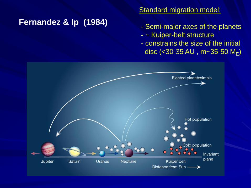
Standard migration model:
- Semi-major axes of the planets
- ~ Kuiper-belt structure
- constrains the size of the initial
disc (<30-35 AU , m~35-50 MΕ)
Fernandez & Ip (1984)
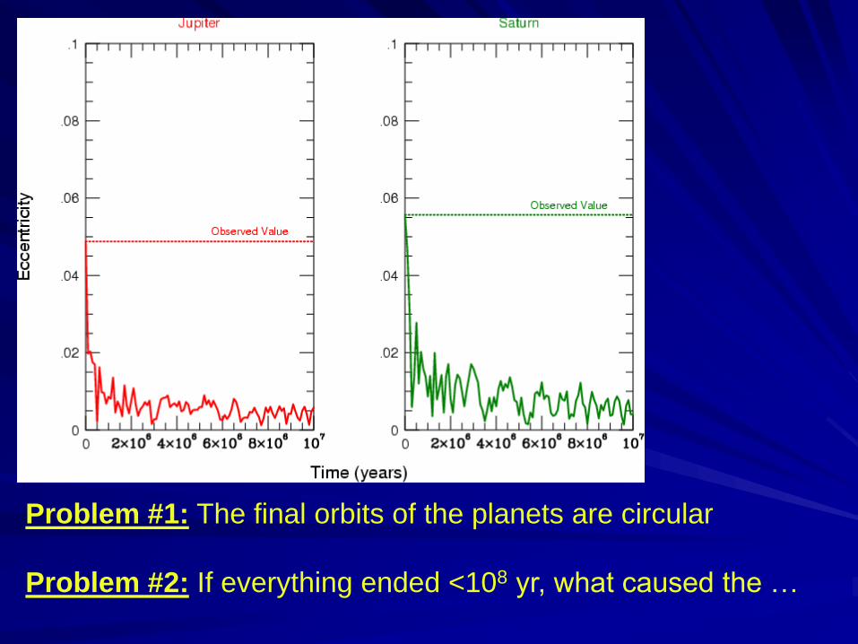
Problem #1: The final orbits of the planets are circular
Problem #2: If everything ended <108 yr, what caused the …

Ein neues Migration Modell
Sind die Planeten weiter auseinander (Neptun bei ~20 AU) -
leichte Migration
Ein kompaktes System kann instabil werden aufgrund
von Resonanzen zwischen den Planeten (und nicht close
encounters) !
Alessandro Morbidelli (OCA, France)
Kleomenios Tsiganis (Thessaloniki, Greece)
Hal Levison (SwRI, USA)
Rodney Gomes (ON-Brasil)
Tsiganis et al. (2005), Nature 435, p. 459
Morbidelli et al. (2005), Nature 435, p. 462
Gomes et al. (2005), Nature 435, p. 466
Nice Model

N-body simulations:
Sun + 4 giant planets + Disc of planetesimals
43 simulations t~100 My:
( e , sinΙ ) ~ 0.001
aJ=5.45 AU , aS=aJ22/3 - Δa , Δa < 0.5 AU
U and N initially with a < 17 AU ( Δa > 2 AU )
Disc: 30-50 ME , edge at 30-35 AU (1,000 – 5,000bodies)
8 simulations for t ~ 1 Gy with aS= 8.1-8.3 AU


Evolution of the planetary system
• A slow migration phase with (e,sinI) < 0.01, followed by
• Jupiter and Saturn crossing the 1:2 resonance eccentricities are
increased chaotic scattering of U,N and S (~2 My) inclinations
are increased
• Rapid migration phase: 5-30 My for 90% Δa

Crossing the 1:2 resonance
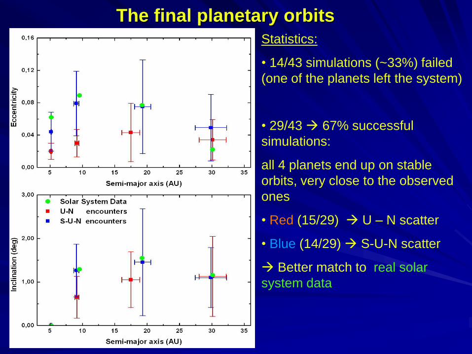
The final planetary orbits
Statistics:
• 14/43 simulations (~33%) failed
(one of the planets left the system)
• 29/43 67% successful
simulations:
all 4 planets end up on stable
orbits, very close to the observed
ones
• Red (15/29) U – N scatter
• Blue (14/29) S-U-N scatter
Better match to real solar
system data

Jupiter Trojans
Trojans = asteroids that share Jupiter’s orbit but librate around the Lagrangian points, δλ ~ ± 60o
We assume a population of Trojans with the same age as the planet
A simulation of 1.3 x 10⁶ Trojans all escape from the system when J and S cross the resonance !!!
Is this a problem for our new migration model?

… No! Chaotic capture in the 1:1 resonance
• The total mass of captured Trojans depends on migration speed
• For 10 My < Tmig < 30 My we trap 0.3 - 2 MTro
This is the first model that explains the
distribution of Trojans in the space of
proper elements ( D , e , I )

The timing of the instability
1 My < Τinst < 1 Gyr
Depending on the density (or
inner edge) of the disc
LHB timing suggests an
external disc of planetesimals in
agreement with the short
dynamical lifetimes of particles
in the proto-solar nebula
• What was the initial
distribution of
planetesimals like ?

We need a huge source of small bodies, which stayed intact for
~600 My and some sort of instability, leading to the bombardment of
the inner solar system
Late Heavy Bombardment
Petrological data (Apollo, etc.) show:
• Same age for 12 different impact sites
• Total projectile mass ~ 6x10²¹ g
• Duration of ~ 50 My
A brief but intense bombardment of the inner solar system,
presumably by asteroids and comets ~ (3.9±0.1) Gyrs ago,
i.e. ~ 600 My after the formation of the planets
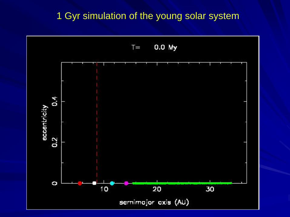
1 Gyr simulation of the young solar system

The Lunar Bombardment
Two types of projectiles:
asteroids / comets
~ 9x10²¹ g comets
~ 8x10²¹ g asteroids
(crater records 6x10²¹ g)
The Earth is bombarded by
~1.8x10²² g comets (water)
6% of the oceans
Compatible with D/H
measurements !

ConclusionsThe NICE model assumes:
An initially compact and cold planetary system with PS / PJ < 2 and an external disc of planetesimals
3 distinct periods of evolution for the young solar system:
1. Slow migration on circular orbits
2. Violent destabilization
3. Calming (damping) phase
Main observables reproduced:
1. The orbits of the four outer planets (a,e,i)
2. Time delay, duration and intensity of the LHB
3. The orbits and the total mass of Jupiter Trojans
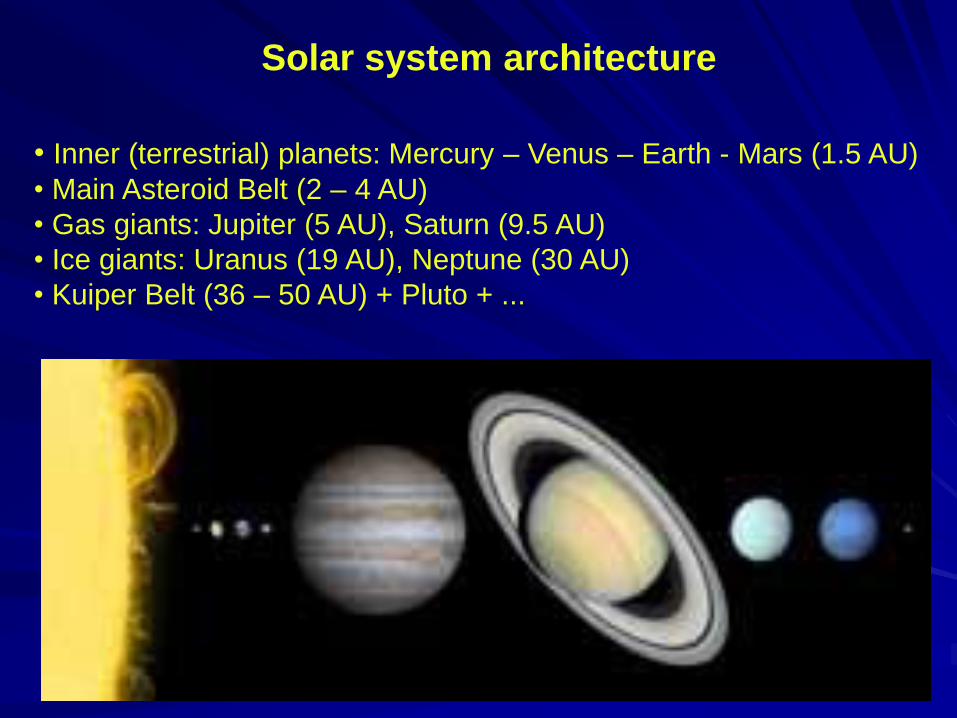
• Inner (terrestrial) planets: Mercury – Venus – Earth - Mars (1.5 AU)
• Main Asteroid Belt (2 – 4 AU)
• Gas giants: Jupiter (5 AU), Saturn (9.5 AU)
• Ice giants: Uranus (19 AU), Neptune (30 AU)
• Kuiper Belt (36 – 50 AU) + Pluto + ...
Solar system architecture

Are there Planets outside the
Solar System ?
First answer :
1992 Discovery of the first Extra-
Solar
Planet around the pulsar
PSR1257+12 (Wolszczan &Frail)
Are there Planets moving around
other Sun-like stars ?

The EXO Planet: 51 Peg b
Mass: M sin i = 0.468
m_Jup
semi-major axis: a =
0.052 AU
period: p = 4.23 days
eccentricity: e = 0
a of Mercury: 0.387 AU
Discovered by:Michel Mayor Didier Queloz

Status of Observations
452 Extra-solar planets
43 Mulitple planetary systems
43 Planets in binaries

Questions
How frequent are other planetary systems ?
Are they like our Solar System ? (no. of planets,
masses, radii, albedos, orbital paramenters , …. )
What type of environments do they have? (atmospheres, magnetosphere, rings, … )
How do they form and evolve ?
How do these features depend on the type of
the central star (mass, chemical composition, age,
binarity, … ) ?
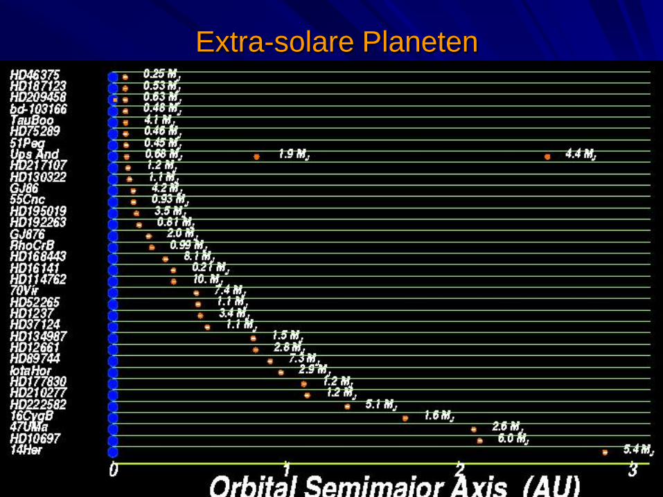
Extra-solare Planeten
ca. 130 Planeten entdeckt
massereich (~Mjup
)
enge Umlaufbahnen
Radialgeschwindigkeits-
messungen

Distribution of the detected Extra-Solar Planets
Mercury Earth Mars
VenusJupiter

Mass distribution

55 Cancri
5 Planeten bei 55
Cnc:
55Cnc d -- the only
known Jupiter-like
planet in Jupiter-
distance
Binary: a_binary= 1000 AU
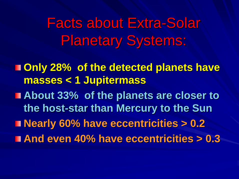
Only 28% of the detected planets have
masses < 1 Jupitermass
About 33% of the planets are closer to
the host-star than Mercury to the Sun
Nearly 60% have eccentricities > 0.2
And even 40% have eccentricities > 0.3
Facts about Extra-Solar
Planetary Systems:

Sources of uncertainty in parameter fits:
the unknown value of the orbital line-of-sight inclination i allows us to determine from radial velocities measurements only the lower limit of planetary masses;
the relative inclination ir between planetary orbital planes is usually unknown.
In most of the mulitple-planet systems, the strong dynamical interactions between planets makes planetary orbital parameters found – using standard two-body keplerian fits – unreliable (cf. Eric Bois)
All these leave us a substantial available parameter space to be explored in order to exclude the initial conditions which lead to dynamically unstable configurations

Binaries
Single Star and Single Planetary Systems
Multi-planetary systems

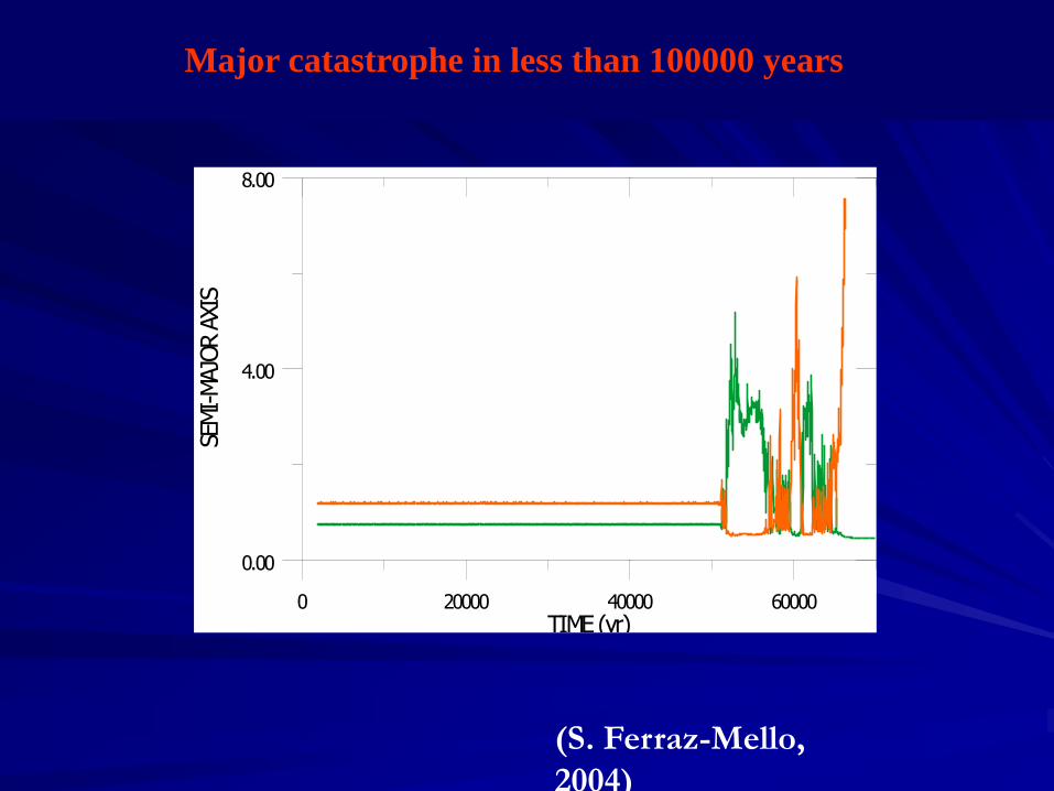
Major catastrophe in less than 100000 years
0 20000 40000 60000TIME (yr)
0.00
4.00
8.00
SEMI-MAJO
R A
XIS
(S. Ferraz-Mello,
2004)

Long-term numerical
integration:
Stability-Criterion:No close encounters within
the Hill‘ sphere
(i)Escape time(ii) Study of the eccentricity:
maximum eccentricity
Chaos Indicators:
Fast Lyapunov Indicator
(FLI)
C. Froeschle, R.Gonczi, E. Lega
(1996)
MEGNO
RLI
Helicity Angle
LCE
Numerical Methods

The Fast Lyapunov Indicator (FLI) (see Froeschle et al., CMDA 1997)
a fast tool to distinguish between regular and chaotic motion
length of the largest tangent vector:
FLI(t) = sup_i |v_i(t)| i=1,.....,n
(n denotes the dimension of the phase space)
it is obvious that chaotic orbits can be found very quickly
because of the exponential growth of this vector in the chaotic
region.
For most chaotic orbits only a few number of primary
revolutions is needed to determine the orbital behavior.

Binaries
Single Star and Single Planetary Systems
Multi-planetary systems
www.univie.ac.at/adg/exostab/
ExoStabappropriate for single-star single-planet system
- Stability of an additional planet
- Stability of the habitable zone (HZ)
- Stability of an additional planet with repect to the HZ
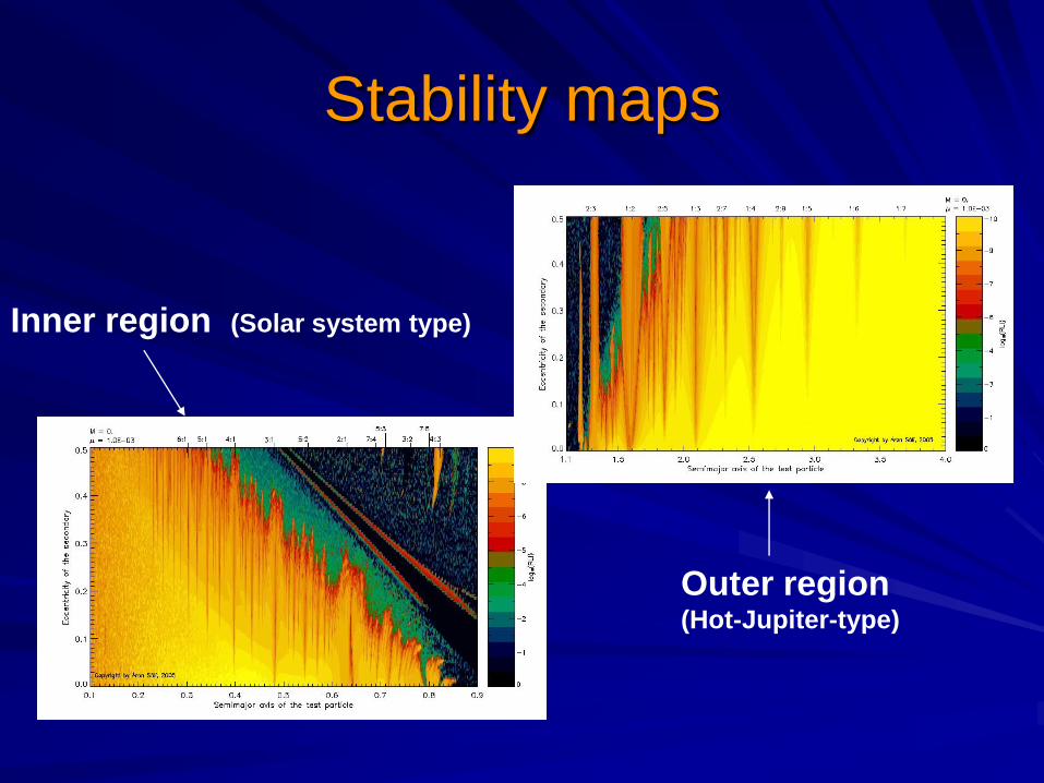
Stability maps
Inner region (Solar system type)
Outer region (Hot-Jupiter-type)

Computationsdistance star-planet: 1 AUvariation of- a_tp:[0.1,0.9] [1.1,4] AU- e_gp: 0 – 0.5- M_gp: 0 and 180 deg- M_tp: [0, 315] deg
Dynamical model: restricted 3 body problem
Methods:
(i) Chaos Indicator:
- FLI (Fast Lyapunov)
- RLI (Relative Lyapunov)
(ii) Long-term computations
- e-max

ANIMATION
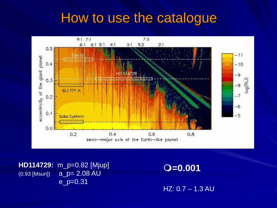
How to use the catalogue
HD114729: m_p=0.82 [Mjup]
(0.93 [Msun]) a_p= 2.08 AU
e_p=0.31
m=0.001
HZ: 0.7 – 1.3 AU
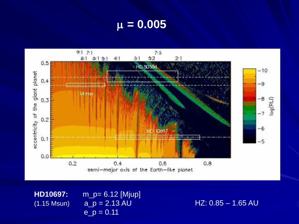
m = 0.005
HD10697: m_p= 6.12 [Mjup]
(1.15 Msun) a_p = 2.13 AU
e_p = 0.11
HZ: 0.85 – 1.65 AU
Multi-planetary systems:

Multi-Planeten Systeme
Stabiliät des Planetensystems muss
überprüft werden

Gliese 876
d c b
a [AU] 0.0208 0.13 0.2078
P[days] 1.9377 30.1 60.94
e 0. 0.27 0.0249
m sin i 0.018 0.56 1.935

CoRoT Exo 7 b

Spacing of Planets -- Hill criterion
Convenient rough proxy for the stability of
planetary systems
In its simpliest form for planets of equal
mass on circular orbits around a sun-like
star

Two adjacent orbits with separation
Dai=ai+1 – ai have to fullfill:

mass-dependency
closer spacing for smaller mass planets

Determination of Planetary Periods:
Using Kepler‘s third law in its log-differential
Form (d ln(P) = 3/2 d ln(a)) obtain the periods Pi
(D Pi / Pi) gives the periodic scaling for the planets-1
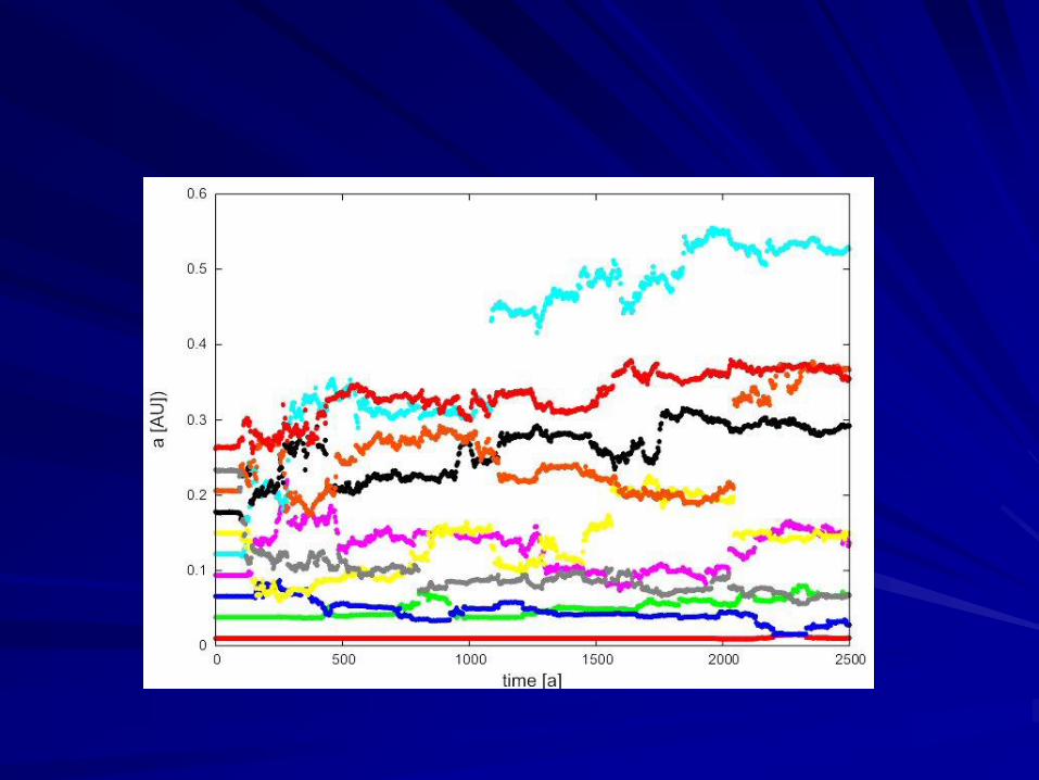
Numerical Study
Fictitious compact planetary systems:
Sun-mass star
up to 10 massive planets (4/17/30 Earth-
masses)
aP= 0.01AU …… 0.26 AU
e, incl, omega, Omega, M: 0
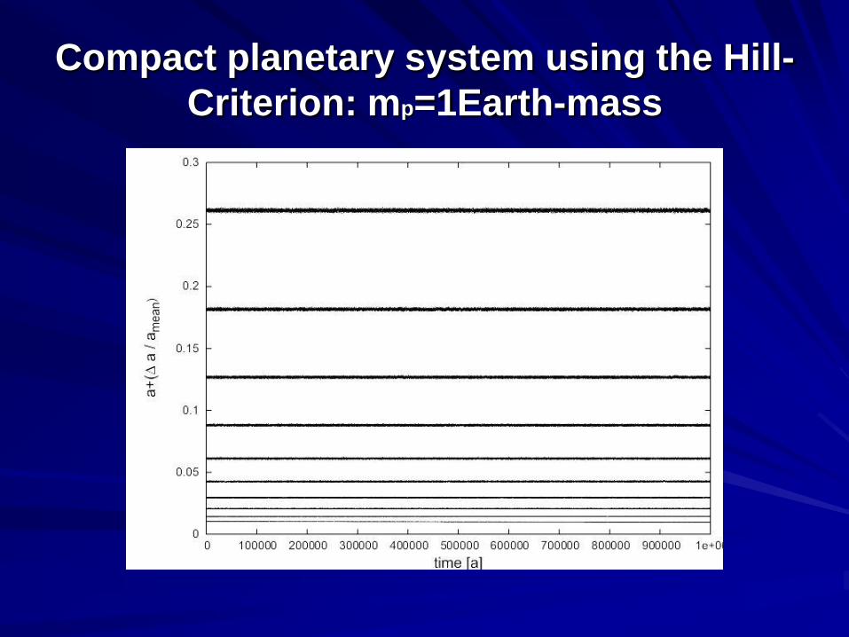
Compact planetary system using the Hill-
Criterion: mp=1Earth-mass
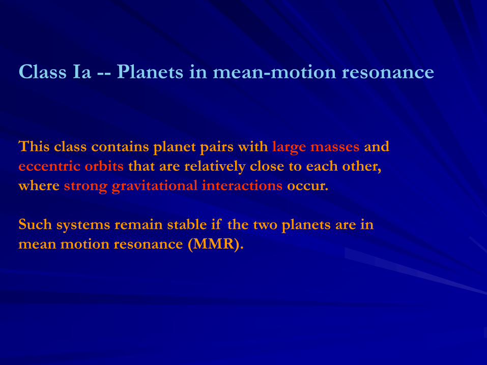
Class Ia -- Planets in mean-motion resonance
This class contains planet pairs with large masses and
eccentric orbits that are relatively close to each other,
where strong gravitational interactions occur.
Such systems remain stable if the two planets are in
mean motion resonance (MMR).

Star Planet mass_P a_P e_P Period
[M_Sun] [M_Jup] [AU] [days]
GJ 876 b 0.597 0.13 0.218 30.38
(0.32) c 1.90 0.21 0.029 60.93
55 Cnc b 0.784 0.115 0.02 14.67
(1.03) c 0.217 0.24 0.44 43.93
HD82942 b 1.7 0.75 0.39 219.5
(1.15) c 1.8 1.18 0.15 436.2
HD202206 b 17.5 0.83 0.433 256.2
(1.15) c 2.41 2.44 0.284 1296.8
How important are the resonances for the long term stability of multi-planet systems?


Gliese 876 HD82943 HD160691
Systems in 2:1 resonance
GJ876 b GJ876c HD82 b HD82 c HD160 b HD160 c
A [AU]: 0.21 0.13 1.16 0.73 1.5 2.3
e: 0.1 0.27 0.41 0.54 0.31 0.8
M .sin i: 1.89 0.56 1.63 0.88 1.7 1.0
[M_jup]
Major catastrophe in less than 100000 years
0 20000 40000 60000TIME (yr)
0.00
4.00
8.00
SEMI-MAJO
R A
XIS
(S. Ferraz-Mello,
2004)

HD 82943 c,b : A case study (S.Ferraz-Mello)
.

HD82943
Aligned
Anti-aligned

S PPA A 1 212
Periastra in the same direction
S PPA A1212
Periastra in opposite directions
Periastra in the same direction
S - P1 - P2
S - A1 - A2
A1 - S - P2
P1 - S - A2
Periastra in opposite directions
S - P1 - A2
S - A1- P2
P1 - S – P2
A1 - S – A2
Equivalent pairs, depending on the
resonance


