Modelling Contact Mechanics with
improved Greenrsquos Function Molecular
Dynamics
Dissertation
zur Erlangung des Grades
des Doktors der Naturwissenschaften
der Naturwissenschaftlich-Technischen Fakultat
der Universitat des Saarlandes
von
Yunong Zhou
Saarbrucken
2020
Tag des Kolloquiums 17 Februar 2021
Dekan Prof Dr Jorn Erik Walter
Berichterstatter Prof Dr Martin H Muser
Prof Dr-Ing Stefan Diebels
Vorsitz Prof Dr-Ing Dirk Bahre
Akad Mitarbeiter Dr-Ing Florian Schafer
iii
Declaration of Authorship
Eidesstattliche Erklarung
Ich erklare hiermit an Eides Statt dass ich die vorliegende Arbeit selbststandig
verfasst und keine anderen als die angegebenen Quellen und Hilfsmittel verwendet
habe
Statement in Lieu of an Oath
I hereby confirm that I have written this thesis on my own and that I have not
used any other media or materials than the ones referred to in this thesis
Einverstandniserklarung
Ich bin damit einverstanden dass meine (bestandene) Arbeit in beiden Versionen
in die Bibliothek der Materialwissenschaft und Werkstofftechnik aufgenommen
und damit veroffentlicht wird
Declaration of Consent
I agree to make both versions of my thesis (with a passing grade) accessible to the
public by having them added to the library of the Material Science and Engineering
Department
DatumDate
UnterschriftSignature
iv
Abstract
Modelling Contact Mechanics with improved Greenrsquos Function
Molecular Dynamics
by Yunong Zhou
Greenrsquos function molecular dynamics (GFMD) is frequently used to solve linear
boundary-value problems using molecular-dynamics techniques In this thesis we
first show that the convergence rate of GFMD can be substantially optimized Im-
provements consist in the implementation of the so-called ldquofast inertial relaxation
enginerdquo algorithm as well as in porting the solution of the equations of motion
into a Fourier representation and a shrewd assignment of inertia GFMD was fur-
thermore generalized to the simulation of finite-temperatures contact mechanics
through the implementation of a Langevin thermostat An analytical expression
was derived for the potential of mean force which implicitly describes the interac-
tion between a hard wall and a thermally fluctuating elastomer GFMD confirmed
the correctness of the derived expression A Hertzian contact was simulated as ad-
ditional benchmark Although the thermally induced shift in the displacement can
be substantial it turns out to be essentially independent of the normal load A fi-
nal application consisted in the test of the frequently made hypothesis that contact
area and reduced pressure are linearly related for randomly rough surfaces The
relation was found to be particularly reliable if the pressure is undimensionalized
with the root-mean-square height gradient
v
Zusammenfassung
Modellierung von Kontaktmechanik mit verbesserter Greenrsquos Function
Molecular Dynamics
by Yunong Zhou
Greenrsquos function molecular dynamics (GFMD) wird haufig verwendet um lin-
eare Randwertprobleme im Rahmen einer Molekulardynamik-Simulation zu losen
In dieser Dissertation zeigen wir zunachst dass die Konvergenzrate von GFMD
substantiell optimiert werden kann Verbesserungen bestehen in der Implemen-
tierung des sogenannten ldquofast inertial relaxation enginerdquo Algorithmus sowie der
Verlagerung der Losung der Bewegungsgleichungen in die Fourier-Darstellung und
einer geschickter Wahl der Massen Desweitern wurde GFMD zur Simulation der
Kontaktmechanik bei endlichen Temperaturen durch Verwendung von Langevin
Thermostaten verallgemeinert Diesbezuglich wurde ein analytischer Ausdruck
fur ein effektives thermisches Potential hergeleitet welches die Thermik repulsiver
Wande implizit beschreibt und durch GFMD bestatigt wurde Als Referenzsys-
tem wurde ein zudem klassischer Hertzrsquoscher Kontakt simuliert Obgleich die
Thermik eine substantielle Verschiebung der Auslenkung bewirken kann erweist
sich die Auslenkung als nahezu unabhrdquoangig von der Normalkraft Schliesslich
konnte als Anwedung auch die haufig fur zufallig raue Oberflachen postulierte lin-
eare Abhangigkeit zwischen realer Kontaktflache und reduziertem Druck getestet
werden Sie gilt vor allem dann wenn der Druck uber dem im echten Kontakt
gemittelte Standardabweichung des Hohengradienten entdimensionalisiert wird
vii
Acknowledgements
First and foremost I would like to express my sincerest appreciation to my super-
visor Prof Dr Martin H Muser for his academic instruction and encouragement
during my thesis work Without his enlightening and patient guidance this thesis
would not have been possible
I would also like to acknowledge the other members of my committee Prof Dr
Stefan Diebels and Prof Dr Dirk Bahre I want to thank each of them for
attending my PhD defense reading my thesis and providing constructive sug-
gestions
I also received invaluable advice from my group mates I want to give special
recognition to Dr Anle Wang for his enthusiastic help on debugging my simulation
codes during these years Dr Hongyu Gao for his suggestions on scientific research
and Dr Sergey Sukhomlinov for his instructions and discussions on the CSMP
course and research
Lastly I would like to thank my parents for all the endless love support and
encouragement in the ups and downs during my years at Saarland University
ix
Content
Declaration of Authorship iv
Abstract v
Zusammenfassung vii
Acknowledgements ix
1 Introduction 1
11 Background 1
12 Approaches to contact mechanics 3
121 Theory approaches 4
122 Numerical approaches 11
13 Research gaps in contact mechanics 13
131 How to locate stable mechanical structure quickly 13
132 What structural parameters affect contact area 14
133 How do thermal fluctuations affect Hertzian theory 15
14 Outline of this thesis 16
2 Optimizations of Greenrsquos function molecular dynamics 19
21 Model and problem definition 20
211 Treatment of elasticity 20
212 Rigid indenters 22
213 Interaction 24
22 Numerical methods 25
221 FIRE GFMD 25
222 Mass-weighted GFMD 26
223 Mass-weighted FIRE GFMD 27
xi
23 Numerical results 28
231 Hertzian indenter 28
232 Randomly rough indenter 32
233 Application to the contact-mechanics challenge 32
24 Conclusion 34
3 Thermal Hertzian contact mechanics 37
31 Model design 38
311 Treatment of elasticity and thermal displacement 38
312 Treatment of interaction 39
32 Thermal GFMD 44
33 Theory 45
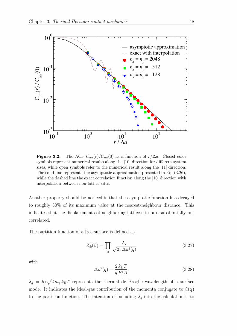
331 The statistical mechanics of a free surface 46
332 Interaction of a thermal elastic surface with a flat wall 49
333 Thermal Hertzian contacts 53
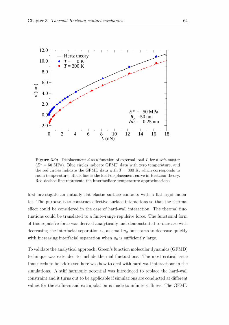
34 Results and analysis 55
341 Flat indenter 55
342 Hertzian indenter 57
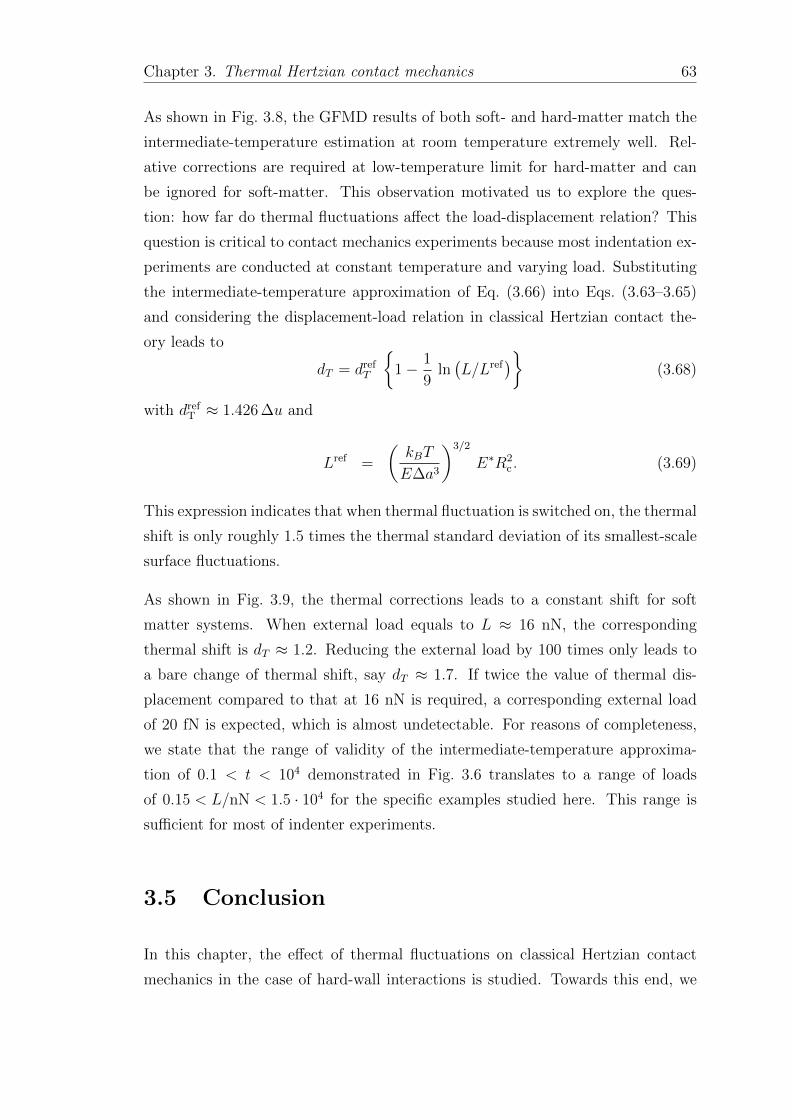
35 Conclusion 63
4 Effects of structural parameters on the relative contact area 67
41 Model design 68
411 Elastic body 68
412 Rigid indenter 68
42 Theory 73
421 Prediction of κ in Persson theory 73
422 Definitions of scalar parameters 74
423 Evaluation of fourth-order invariants 78
43 Results 79
431 On the accurate calculation of ar and κ 79
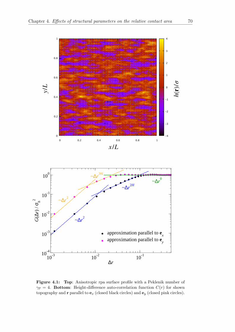
432 Isotropic rpa surfaces 81
433 Anisotropic rpa surfaces 86
434 Isotropic height-warped surfaces 88
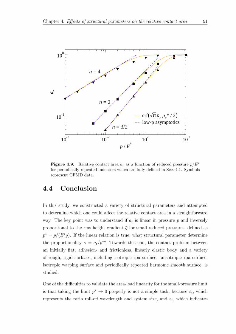
435 Periodically repeated smooth indenters 89
44 Conclusion 91
5 Thermal effects on the pull-off force in the JKR model 95
xii
51 Model design 96
52 Method 98
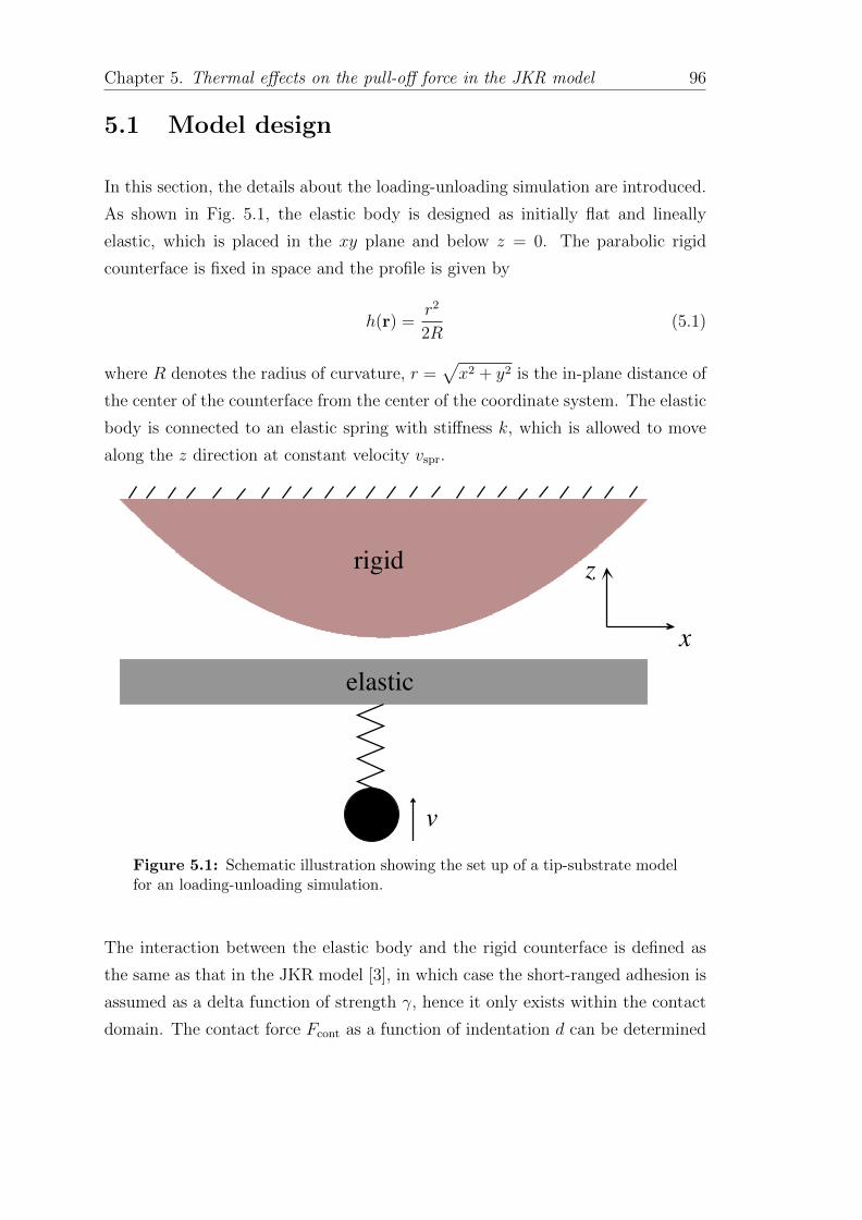
53 Results 100
54 Conclusions 104
6 Conclusions and outlook 105
List of Figures 107
List of Tables 113
Bibliography 114
GFMD documentation 129
A1 Introduction 129
A11 Basic idea of GFMD 129
A12 Source code structure 130
A13 Basic running 130
A14 Visualization 132
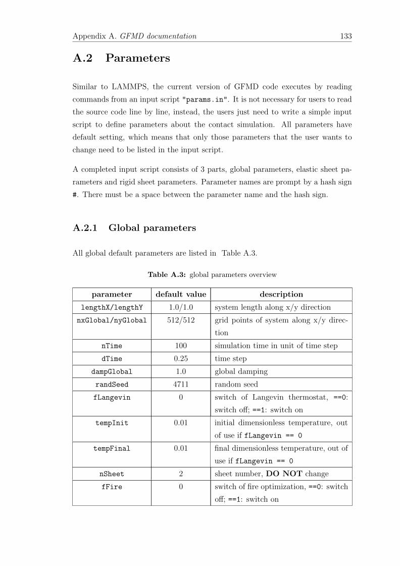
A2 Parameters 133
A21 Global parameters 133
A22 Rigid sheet parameters 134
A23 Elastic sheet parameters 140
A24 Read old configuration 142
A3 Interaction 142
A31 Hard-wall constraint 143
A32 Adhesion interaction and hard-wall constraint 144
A33 Adhesion interaction and short-ranged repulsion 145
A4 Examples 145
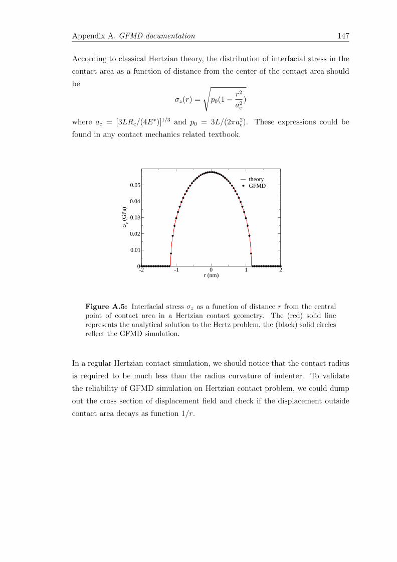
A41 Hertzian contact problem with hard-wall constraint 146
A42 Hertzian contact problem with adhesion interaction 149
A43 Rough surface contact problem with adhesion interaction 150
A44 Hertzian contact problem with Morse potential 152
A5 Optimizations 153
A51 Fast inertia relaxation engine (FIRE) 153
A52 Mass-weighted GFMD 155
A53 FIRE mass-weighting GFMD 156
xiii
Chapter 1
Introduction
11 Background
Contact mechanics is a study that focuses on the deformation of elastic bodies
when they contact each other The pioneering work on contact mechanics was
another important contribution by the famous German physicist Heinrich Hertz
following his confirmation of the existence of electromagnetic waves In 1882
Hertz solved the adhesion- and frictionless contact problem of two linear elastic
spheres analytically [1] So far the analytical work managed by Hertz on contact
mechanics still remains the theoretical basis for many practical contact problems
in engineering and has a profound influence on the development of mechanical
engineering and tribology in particular [2] Since then the study of contact me-
chanics has made great progress Johnson et al strived to include short-ranged
adhesion into classical Hertzian contact problem the resulting theory work was
known as Johnson-Kendall-Roberts (JKR) model [3] Another similar work was
managed by Derjaguin et al in which the interaction was replaced by long-ranged
force It is known as Derjaguin-Muller-Toporov (DMT) model [4]
All of the theoretical works mentioned above considered only contacts of smooth
bodies However there is no such an absolutely smooth surface in the world
even a highly polished surface will have many microscopic asperities Therefore
accurately evaluating the true contact situation such as knowing the true contact
area of rough surface is significant for many engineering applications Currently
the dominant rough contact theories can be broadly divided into the following
two categories (1) multiple asperity contact model pioneered by Greenwood and
Williamson in their Greenwood-Williamson (GW) model (2) scaling theory for
randomly rough contacts proposed by Persson which is also known as Persson
1
Chapter 1 Introduction 2
theory More details about these two theories will be outlined in the following
section
In terms of numerical methods the boundary element method (BEM) and the
finite element method (FEM) provide effective approaches of solving contact me-
chanics problems with complex boundary conditions However for numerical sim-
ulations of contact problems that consider small scale roughness for the purpose of
practical interest a fine surface grid is necessary for the numerical contact analy-
sis As a result rough surface contact problems generally need to be conducted on
grids with a large number of nodes Solution of such huge systems of equations is
extremely time-consuming even on high speed computers Thus it is particularly
meaningful to study the optimization of numerical simulations Polonsky et al
proposed a conjugate-gradient (CG) based method combined with the multi-level
multi-summation (MLMS) algorithm to obtain a fast converge contact mechanics
solver [5] Bugnicourt et al developed a similar toolbox based on CG method
while the MLMS algorithm was replaced by fast Fourier transform (FFT) algo-
rithm [6] Campana and Muser developed Greenrsquos function molecular dynamics
(GFMD)[7] which as other boundary value method do allows us to simulate the
linear elastic response of contact problem in terms of the displacement in the top
layer of elastic solid
So far contact mechanics is adopted in a wide range of applications ranging
from traditional mechanical engineering systems microelectromechanical systems
(MEMS) and biological systems
In the domain of classical mechanical engineering the performance of tires gaskets
sealings braking systems and so on are closely related to their contact mechanics
A commonly used example is the leakage problem of seal in the water tap or
hydraulic system The gap and the relative contact area between the contact solids
play a critical role in this issue Many studies tried to understand how external
load and surface roughness affect the gap and relative contact area [8ndash11] These
studies could in turn make it possible to design a more reliable mechanical device
to reduce leakage Even though a seal is only a small component it deserves a lot
of attention In the event of leakage in the hydraulic part the reliability would be
reduced and the oil would be wasted In some instances it could also trigger an
undesirable accident such as the Challenger disaster
Chapter 1 Introduction 3
The mechanical properties of the contact process in MEMS is another substan-
tial topic in contact mechanics MEMS is a modern technology which combines
microelectronics and mechanical engineering It has been broadly employed in a
number of applications which profoundly affect peoplersquos daily life A classical
application is a pressure sensor which is a kind of device that receives pressure
as an input signal and outputs electrical signals as a function of the input pres-
sure In general a pressure sensor could be modeled as an elastic body with finite
thickness deposited on a rigid nominally flat substrate eg silicon Its operating
scale is in the micrometer range There are pieces of evidences showing that the
surfaces cannot be regarded as smooth [12 13] Additionally due to the sizable
surface-volume ratio in MEMS devices surface force eg van der Waals forces
start to play an important role in adhesion Vast studies have demonstrated that
surface roughness is a prominent factor reducing in adhesion [14 15] At this
point it is interesting to study how surface roughness and adhesion contribute
to the output electrical signal in a pressure sensor which is still in the range of
contact mechanics study On the other hand some studies have demonstrate that
the thermal effect could significantly affect van der Waals interactions [16ndash18] At
this point considering the performance of MEMS devices in different conditions
such as a wide range of temperature it is also interesting to include the effect of
thermal fluctuation into a contact mechanics treatment
12 Approaches to contact mechanics
As mentioned in the previous section the classical Hertzian contact theory which
was conceived in 1881 established the groundwork for the field of contact me-
chanics In the next two hundred years a diverse understanding of rough surfaces
was developed and a number of theories of rough contact mechanics were formu-
lated based on this understanding The most dominant of these are GW model
(multiple asperity model) and Persson theory (scaling theory for randomly rough
contact) Since this thesis mainly focuses on Hertzian and random rough surface
contacts this section will review these methods briefly On the other hand nu-
merical techniques for the solution of contact problem such as GFMD will also
be discussed
Chapter 1 Introduction 4
121 Theory approaches
Single asperity contact theory
The theory work conducted by Hertz is commonly considered to be the beginning
of modern contact mechanics study [1] He solved the adhesion- and frictionless
normal contact problem at small load between two elastic sphere bodies with
Youngrsquos modulus E1 and E2 Poisson ratio ν1 and ν2 and radius curvature R1 and
R2 This contact problem is equivalent to the contact of a rigid parabolic indenter
with radius curvature Rc and a flat half-space elastic surface with effective modulus
Elowast if satisfying the following relation
1
Rc
=1
R1
+1
R2
and1
Elowast=
1minus ν21
E1
+1minus ν2
2
E2
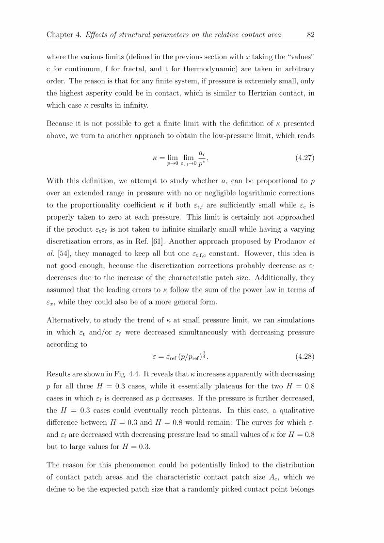
A typical Hertzian contact model is drawn in Fig 11
elastic layer
x
y
Figure 11 Hard-wall constraint elastic solid of finite thickness compressedby a parabolic indenter The dotted line shows the associated stress profile
The parabolic indenter is given by
h(r) =r2
2Rc
Chapter 1 Introduction 5
where Rc is the radius of curvature and r =radicx2 + y2 is the in-plane distance
of the center of the indenter from the origin of the coordinate system The gap
g(x y) represents the distance between elastic solid and rigid parabolic indenter
which reads
g(x y) = h(r)minus u(x y)
where u(x y) is defined as the displacement of elastic solid The hard-wall con-
straint is applied in Hertzian contact theory which indicates that the indenter
cannot penetrate the elastic layer it reads
g(x y) ge 0
Hertzian theory predicts that the contact area ac increases with external force FN
which reads
a3c =
3FNRc
4Elowast(11)
The stress profile in the contact area is given below
σ(r) = σ0
[1minus
(r
ac
)2]12
(12)
where σ0 = 3FN(2πa2c) is the maximum (compressive) stress
The traditional Hertz theory only included the repulsion force induced by the
squeezing of contact bodies This approach is applicable to macro-scale contact
problems However the surface force which is neglected at the macro-scale
can become effective at micrometer or even smaller scales This surface force
stems from van der Waals forces Because surface forces play an essential part in
many technical applications and biological systems it is necessary to generalize
the nonoverlap Hertzian theory to adhesive contact theory
Towards this end Johnson et al reinvestigated the Hertzian contact problem
by considering adhesive interaction which is also known as JKR model [3] JKR
theory included adhesion as short-range interaction which means JKR theory only
considered the adhesion within the contact area between two bodies to predict the
force response of the system The adhesion outside the contact area is neglected
At this point Johnson et al derived the expression of the contact area ac as a
Chapter 1 Introduction 6
function of external force FN to be
a3c =
3Rc
4Elowast
(FN + 3γπRc +
radic6γπRcFN + (3γπRc)2
) (13)
where γ is the energy per unit contact area When γ = 0 this expression reduces
to Hertzian theory as shown in Eq (11) In the JKR model an additional force
Fp is required to separate the contact bodies this pull-off force is predicted as
Fp = minus3
2γπRc (14)
Unlike the JKR model Derjaguin et al treated adhesion as a long-range interac-
tion and neglected the effect of adhesion on the deformation of elastic bodies [4]
As a result adhesion force behaves as an external load that is independent of the
contact area This model is known as the DMT model for which the contact area
is predicted as
a3c =
3Rc
4Elowast(FN + 2γπRc) (15)
When contact area ac = 0 the resulting pull-off force is given by
Fp = minus2γπRc (16)
Apparently the estimation of the pull-off force in DMT theory remains different
from that in JKR theory There was a longtime discussion about the way to explain
this divergence Tabor recognized that the JKR model and DMT model describe
the opposite limits of short-range and long-range interaction [19] He demonstrated
that the opposition between these two theories could be fixed by introducing a
dimensionless parameter microT which is now known as Tabor parameter
microT =
[Rcγ
2
Elowast2z30
] 13
(17)
where z0 characterizes the range of adhesion Essentially the Tabor parameter
could be interpreted as the ratio of elastic deformation induced by adhesion and
the effective range of this surface force The contact is close to JKR limit when
microT is large (microT gt 5) while close to DMT limit when microT is small (microT lt 01) [20]
Chapter 1 Introduction 7
Contact mechanics theory of nominally flat surfaces
Classical single-asperity contact mechanics assumes that the contact surface is
geometrically smooth However even though the real surface appears to be flat
on a macro-scale it is rough on the micro-scale Standing by a practical point
of view the Hertzian theory and the JKR and DMT model cannot meet the
requirement of mechanical engineering demands In this case various models
based on roughness representation are developed to describe the contact behavior
between the elastic surface and rough indenter One of the pioneering works is
developed by Greenwood and Williamson known as the GW model [21]
GW model solved the contact between an ideally flat surface and a nominally flat
surface with many asperities In this model numerous asperities are distributed
on a nominal flat plane All asperity heights follow a specific height distribution
function for example a Gaussian distribution Each asperity is treated as a
classical Hertzian model with identical radius curvature however interactions
between asperity is neglected In this case the rough surface can be determined
by three statistical parameters the standard deviation of asperity height σG a
characteristic asperity radius RG and the surface density of asperities ηG Suppose
the separation between two surfaces is d the height of a certain asperity is s The
penetration is given by sminusd Some asperities would be contact at this height the
probability is
Pr(s gt d) =
int infin
d
φlowast(s)ds (18)
where φlowast(s) is the probability distribution function of the asperity height Suppose
the asperity height follows Gaussian distribution φlowast(s) is normalized to standard
Gaussian distribution to simplify the calculation therefore
φlowast(s) =1radic2πeminus
s2
2 (19)
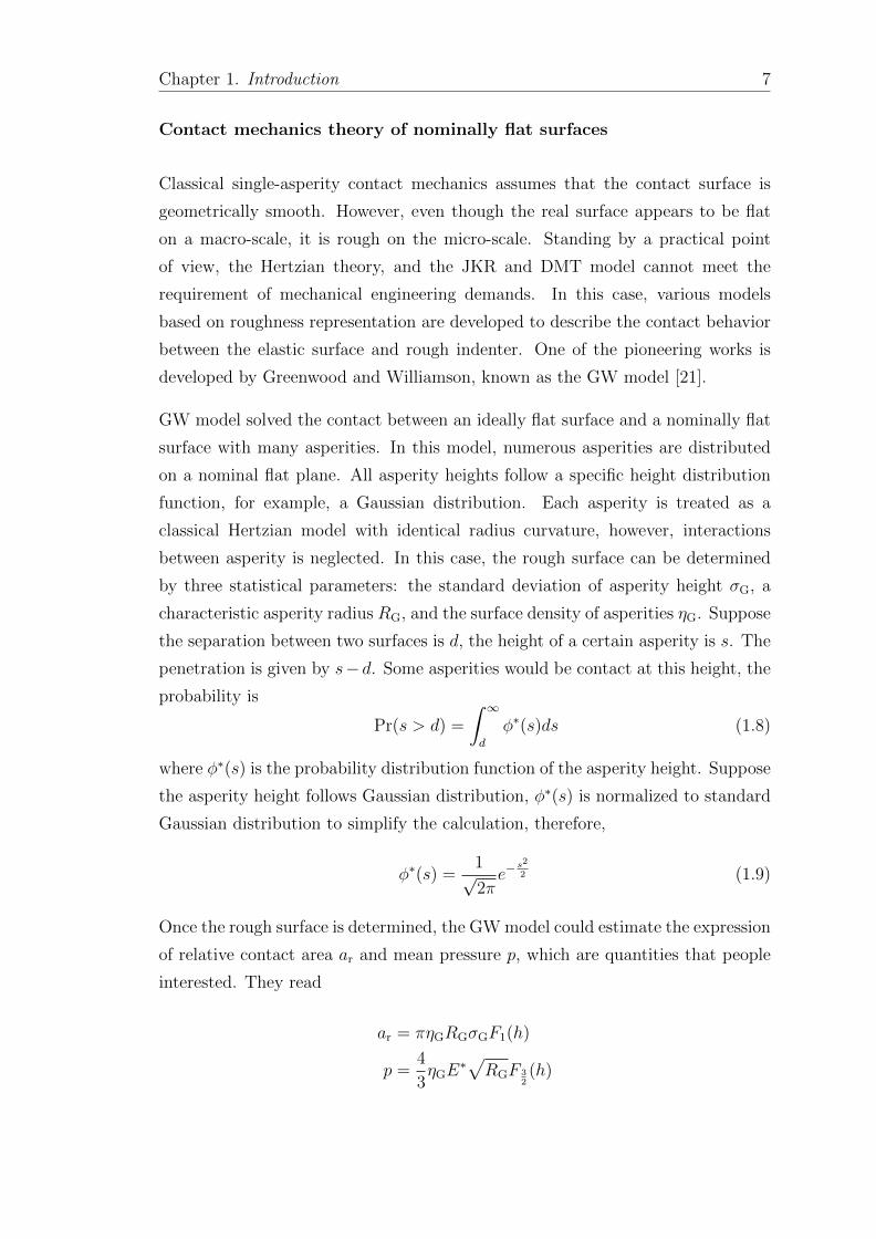
Once the rough surface is determined the GW model could estimate the expression
of relative contact area ar and mean pressure p which are quantities that people
interested They read
ar = πηGRGσGF1(h)
p =4
3ηGE
lowastradicRGF 3
2(h)
Chapter 1 Introduction 8
where
Fn(h) =
int infin
h
(sminus h)nφlowast(s)ds
and h = dσG
The GW model has been extensively used since it was published Additionally
many studies made an effort to extend the utility of the GW model For example
Fuller and Tabor applied the JKR model to each asperity instead of the tradi-
tional Hertzian contact model so that the GW model was able to include adhesion
interaction [22]
Despite the successfully widespread use of the GW model it still suffers from limi-
tations [23] First it is still unclear that the statistical construction of the random
surface is correct Second the GW model assumed that the surface roughness
was only on a single length-scale This assumption leads to an identical asperity
radius of a random surface which remains physically meaningless since the radius
is obviously affected by the resolution of the measuring apparatus [24] Third
the GW model neglected the elastic coupling between asperities In fact as men-
tioned by Campana Muser and Robbins any bearing area model such as the
GW model produces a very poor contact auto-correlation function (ACF) which
reads Cc(q) prop ∆rminus2(1+H) while the correct ACF should be Cc(q) prop ∆rminus(1+H) [25]
Persson developed an alternative approach to contact mechanics that was able
to overcome many shortcomings of the GW model [24 26 27] As mentioned
by Archard the stochastic parameters of random surfaces are dominated by the
resolution of the measurement apparatus [28] At this point the rough surface in
the Persson theory was designed to be self-affine fractal A fractal surface has the
property that the roughnessrsquos statistical property remains identical if the length
scale changes This kind of surface is defined by the surface roughness power
spectrum C(q) it reads
C(q) = C(q0)
(q
q0
)minus2(H+1)
(110)
where H is the Hurst exponent which is related to the fractal dimension via
Df = 3 minus H q0 indicates an arbitrary reference wave number Usually q0 is
chosen to be identical with qr = 2πλr where λrs represents the roll-off and
shortest wavelength respectively In reality the random surface cannot be self-
affine over all length scales Therefore the power spectrum should be within a
Chapter 1 Introduction 9
range of 2πλr le q le 2πλs an idealized power spectrum is depicted in Fig 12
A variety of surfaces are demonstrated by experiments that follow this feature
[24 26 29 30] The Fourier transform of a random roughness surface profile
102 103
q10-4
10-3
10-2
10-1
100
C(q
) C
(qr)
qs
qr
Figure 12 Surface roughness power spectrum of a surface which is self-affinefractal for 2πλr le q le 2πλs Dash line indicates that those wavenumberscannot be detected by measurement apparatus
satisfying the random-phase approximation is defined by
h(q) =radicC(q)e2πir(q) (111)
where r(q) is a uniform random number on (0 1) The resulting surface height
h(r) of random roughness surface is given by the inverse Fourier transform of h(q)
A typical random surface produced from the power spectrum shown in Eq 110 is
depicted in Fig 13
The basic idea of Persson theory is to understand how the pressure distribution
Pr(p ζ) changes as the magnification ζ = qqr is increased where qr = 2πλr
indicates the smallest wavenumber that could be detected Additionally when
observing the random surface under the magnification ζ only those asperities
Chapter 1 Introduction 10
equilPos0dat
0 02 04 06 08 1
0
02
04
06
08
1
0
002
004
006
008
01
012
014
Figure 13 Height profile of random roughness surface with self-affine propertyfor λrL = 12
which wavenumber smaller than q could be detected In a special case say ζ =
1 no asperity could be identified which means direct contact of two smooth
planes [24 31] On the other hand when ζ = qsqr this magnification takes
maximum where qs = 2πλs is the maximum wavenumber that measurement
apparatus could detect
The starting point in Persson theory is to assume that full contact is satisfied in
any magnification At this point a probability density function P (p ζ) is defined
where p is pressure After that a diffusion function is derived to describe the
probability function changing with magnification ζ It is given by
partP
partζ= f(ζ)
part2P
partp2(112)
Chapter 1 Introduction 11
where f(ζ) is a function that includes all information about the random roughness
surface
f(ζ) =π
4
(E
1minus ν2
)2
qrq3C(q) (113)
Because the contact problem degenerates to the contact of two smooth surfaces
when ζ = 1 the initial condition of diffusion function should satisfy
P (p 1) = δ(pminus p0) (114)
where δ(middot) is the Dirac delta function p0 represents nominal contact pressure
Under the assumption of full contact and no adhesion included the boundary
condition of diffusion function should be
P (0 ζ) = 0 (115)
The diffusion function could be solved analytically with the boundary condition
and the initial condition given above The relative contact area is given by
ar = erf
(p0
2radicG
)(116)
where
G(ζ) =π
4
(E
1minus ν2
)2 int ζqr
qr
dqq3C(q) (117)
is identical to the standard deviation of the stress in full contact Compared with
the GW model Persson theory is more accurate when the contact area is very
large
122 Numerical approaches
Theoretical approaches to contact mechanics encounter difficulties when the con-
tact is coupled with too many factors such as temperature and humidity In this
case physical experiment and numerical simulation would be more convenient
ways to access contact mechanics studies Consequently these two approaches
have attracted a lot of attention [32ndash34] However the experimental approach to
contact mechanics to some extent still suffers limitations First the experiment
apparatus can only work for contact mechanics problems with a specific strategy
namely the applicability is limited Second in most cases it is cost-consuming
Chapter 1 Introduction 12
to set up and maintain the experiment apparatus Therefore considering the fast
development of computer technology in the past decades it is urgent to develop a
powerful numerical modeling technique to benefit the study of contact mechanics
The finite element method (FEM) is one of the dominating numerical techniques
to solve partial differential equations (PDE) in combination with boundary con-
ditions this kind of problem is known as boundary value problem (BVP) Gener-
ally a contact mechanics problem can be mapped onto BVP without much effort
Therefore the contact mechanics problem could also be investigated within the
framework of FEM A series of studies of contact mechanics with FEM approach
has demonstrated its reliability [35ndash37]
However when investigating the linear elastic contact problem although FEM
can also solve such problems GFMD which is a BEM is more efficient GFMD
allows us to simulate the linear elastic response of a semi-infinite or finite-thickness
elastic solid to an external load or generally boundary condition acting on the
surface [7 38] During the last decades GFMD has been used extensively to solve
those contact mechanics of elastic solids with either simple parabolic or random
roughness surfaces [39ndash42] The advantage of GFMD is that it only propagates the
displacement of the top layer As a result a relatively large system can be resolved
and the local potential energy minimum could be located more quickly than all-
atom simulations and FEM Most of the simulations in this thesis is concerned
with stable mechanical structures Therefore the damping term is introduced to
the dynamics such that the minimum of potential energy could be quickly located
with a well-chosen damping parameter
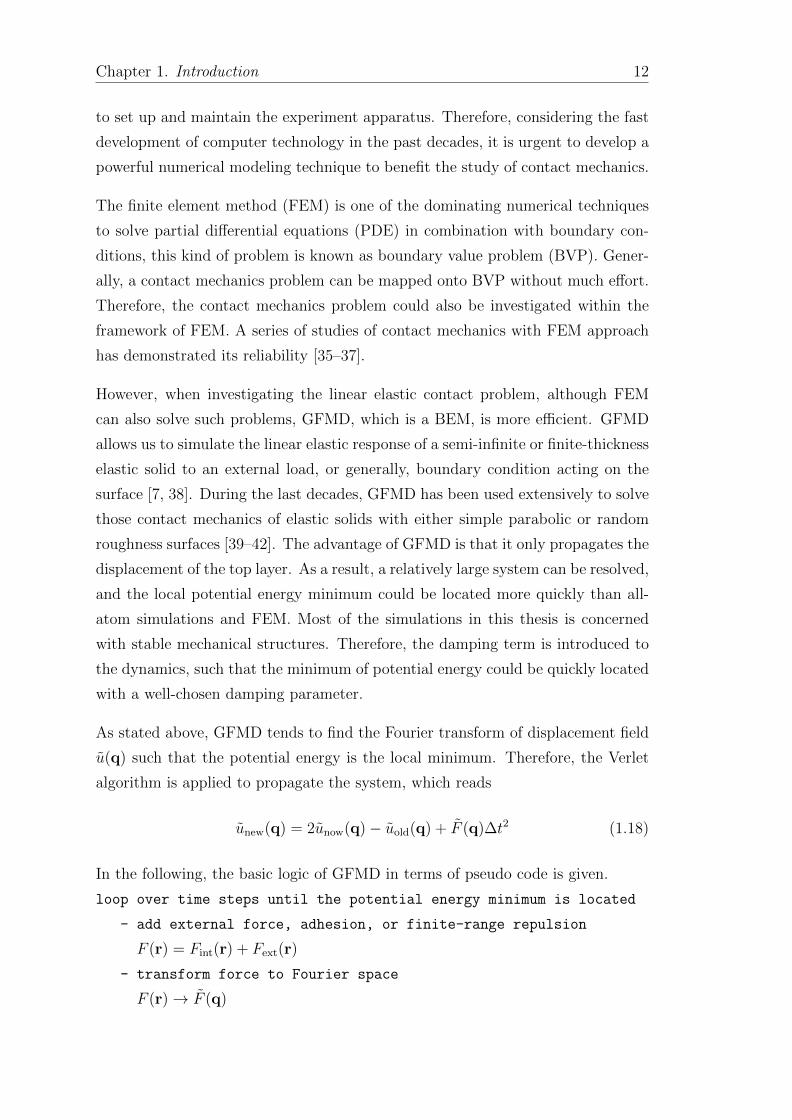
As stated above GFMD tends to find the Fourier transform of displacement field
u(q) such that the potential energy is the local minimum Therefore the Verlet
algorithm is applied to propagate the system which reads
unew(q) = 2unow(q)minus uold(q) + F (q)∆t2 (118)
In the following the basic logic of GFMD in terms of pseudo code is given
loop over time steps until the potential energy minimum is located
- add external force adhesion or finite-range repulsion
F (r) = Fint(r) + Fext(r)
- transform force to Fourier space
F (r)rarr F (q)
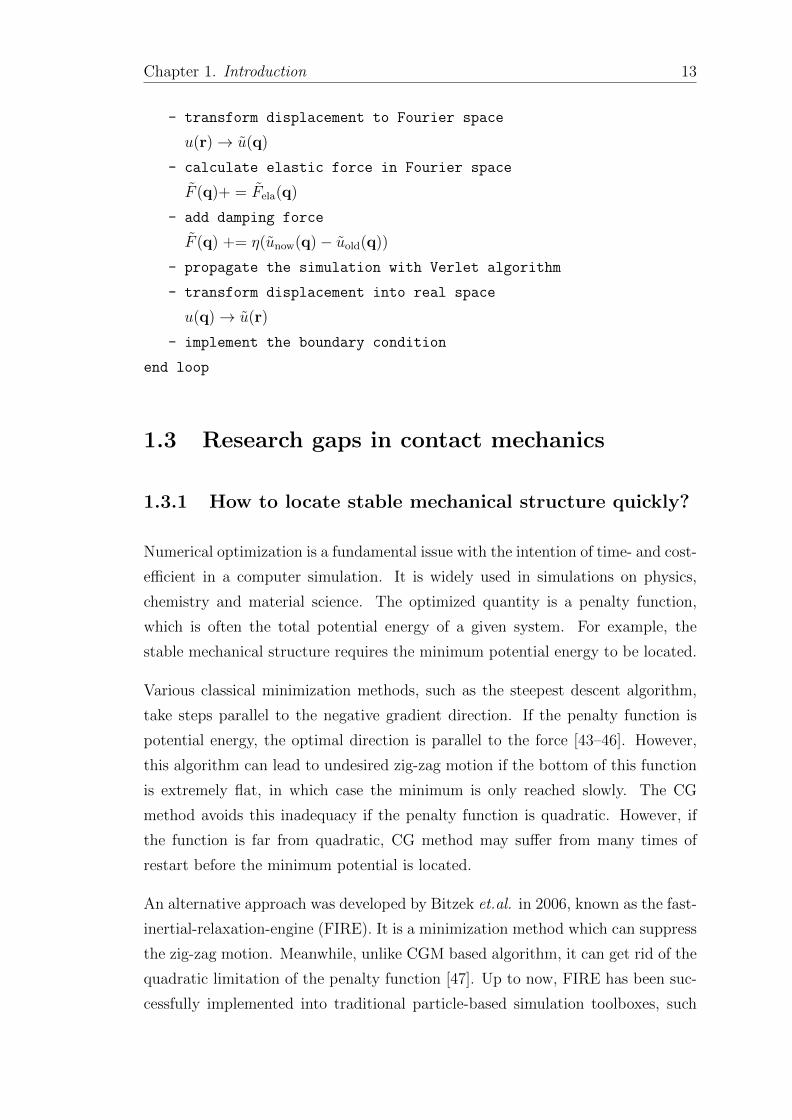
Chapter 1 Introduction 13
- transform displacement to Fourier space
u(r)rarr u(q)
- calculate elastic force in Fourier space
F (q)+ = Fela(q)
- add damping force
F (q) += η(unow(q)minus uold(q))
- propagate the simulation with Verlet algorithm
- transform displacement into real space
u(q)rarr u(r)
- implement the boundary condition
end loop
13 Research gaps in contact mechanics
131 How to locate stable mechanical structure quickly
Numerical optimization is a fundamental issue with the intention of time- and cost-
efficient in a computer simulation It is widely used in simulations on physics
chemistry and material science The optimized quantity is a penalty function
which is often the total potential energy of a given system For example the
stable mechanical structure requires the minimum potential energy to be located
Various classical minimization methods such as the steepest descent algorithm
take steps parallel to the negative gradient direction If the penalty function is
potential energy the optimal direction is parallel to the force [43ndash46] However
this algorithm can lead to undesired zig-zag motion if the bottom of this function
is extremely flat in which case the minimum is only reached slowly The CG
method avoids this inadequacy if the penalty function is quadratic However if
the function is far from quadratic CG method may suffer from many times of
restart before the minimum potential is located
An alternative approach was developed by Bitzek etal in 2006 known as the fast-
inertial-relaxation-engine (FIRE) It is a minimization method which can suppress
the zig-zag motion Meanwhile unlike CGM based algorithm it can get rid of the
quadratic limitation of the penalty function [47] Up to now FIRE has been suc-
cessfully implemented into traditional particle-based simulation toolboxes such
Chapter 1 Introduction 14
as LAMMPS This fact indicates that FIRE should also work for the solution of
partial-differential equations (PDEs) The reason is that the solution of PDEs can
be mapped onto a MD problem after discretization of the variable space Simi-
larly FIRE also works for boundary-value problems (BVPs) Therefore it could
also benefit the solution of contact mechanics simulation which could be trans-
lated to a boundary-value problem (BVP) GFMD is a technique that allows such
BVPs to be addressed within the framework of MD [7 38 48] Although GFMD
has been widely used in contact mechanics simulations there is little research on
optimization for this technique There is also no research on the implementation
of FIRE for the optimization of GFMD
132 What structural parameters affect contact area
Another issue regarding the real contact area has received considerable critical
attention especially the relation between relative contact area ar and pressure p
in nominally flat linearly elastic contact [21 36 49ndash51] It has been reported many
times that the relative contact area ar increases with pressure from very small but
non-zero ar up to ar asymp 01 in randomly rough surface contact simulations [35 51ndash
54] This randomly rough self-affine surface is defined by a height power spectrum
C(q) which reads C(q) prop qminus2(1+H) where H is the Hurst exponent which is a
quantity that correlates to the fractal dimension via Df = 3minusH q is the magnitude
of wave vector q The phases of the randomly rough surface height in Fourier
space are independent random numbers that are uniformly distributed on (0 2π)
such that the surface is fully defined as the random phase approximation (rpa)
surface Persson theory managed to explain the linearity of area-pressure relation
up to roughly 10 relative contact area on Taylor expanding of Eq (116) if the
randomly rough surface is rpa [8 24] Unlike the bearing-area model Persson
theory also finds an accurate pressure-dependence of the interfacial stiffness along
with an accurate distribution function of the interfacial separation [27 34 54ndash57]
Although it is argued that the area-pressure relation should be linear for randomly
rough surfaces several indications suggest that this linearity is not accurate es-
pecially when the external load is fairly small so that only a meso-scale patch in
contact region is measured [58] In fact as Yastrebov and coworkers reported
even though several asperities were in contact the area-pressure relation still de-
viates from linearity [59] However the ratio of system size and short-wavelength
Chapter 1 Introduction 15
cutoff was fixed in their simulations in which case the deviation from the linear-
ity may not convincing To make it clear Nicola etal carefully studied (1+1)
dimensional adhesionless contact between an elastic body and a randomly rough
surface remarkable logarithmic corrections to the area-pressure linearity were re-
ported [42] After that a similar study which was (2+1) dimensional adhesive
contact between an elastic solid and a randomly rough self-affine surface was con-
ducted [60] In this study a clearly sublinear scaling was found However since
they studied the adhesive contact problem the deviation from linearity could stem
from the adhesive hysteresis
It is still remain unclear how the Hurst exponent affects the linear pre-factor of
area-load relation Some studies claimed that this pre-factor is closely correlated
with the Nayak parameter at fixed pressure [59 61 62] However as mentioned
above the ratio of system size and short-wavelength cutoff was fixed in their
simulations as a result the logarithmic relation between contact area and the
Nayak parameter is not plausible In fact the dependence of the pre-factor on
the Nayak parameter turns out to be weak if the surface is not in the domain of
ideally random rough To make it clear let us consider two thought experiments
regarding the contact problem of nominally flat surfaces In the first experiment
we arbitrary modify the height profile of the rough indenter in non-contact zone
but make sure that all modified points are below the elastic body In such a way
the contact area remain unchanged while the Nayak parameter could have shifted
by orders of magnitude In the second experiment we modify the randomly rough
surface such that the peaks are blunt and the valleys are steep In this case for a
given pressure the relative contact area should be large After then the indenter
is flipped around and the resulting contact area would decreased while the Nayak
parameter remain unchanged As a result the correlation between the Nayak
parameter and the pre-factor is not convincing especially when the rpa surface is
not considered
133 How do thermal fluctuations affect Hertzian theory
As mentioned above many mechanical applications such as gaskets braking sys-
tems and pressure sensors need to be considered for their performance at different
temperatures because temperature can affect the mechanical contact in numerous
Chapter 1 Introduction 16
ways Continuum contact mechanics theories such as Hertzian theory often ig-
nore the effect of thermal fluctuations This approximation is reasonable when
applying the theory to macro-scale problems However if the contact problem
is micro-scale or even smaller the approximation could lead to noticeable er-
rors for the load-indentation relation when two bodies are pressed against each
other [63 64] Temperature can affect mechanical contacts and their interpreta-
tion in numerous other ways For example the presence of thermal noise generally
impedes an unambiguous definition of contact area [65ndash69] In addition consider-
ing the van der Waals force between contact bodies significant reduction of pull-off
force with increasing temperature was observed in atomic-force microscope (AFM)
experiment [16] It is possible that thermal surface fluctuations which were not
included in the modeling of temperature effects on tip depinning are responsible
for a significant reduction of effective surface energy and thereby for a reduction
of the depinning force In fact it has been shown that thermal fluctuations limit
the adhesive strength of compliant solids [70] Finally in the context of colloid
science it may well be that thermal corrections have a non-negligible effect on the
surprisingly complex phase diagram of Hertzian spheres [71] It is therefore cer-
tainly desirable to model the effect of thermal fluctuations in a variety of contact
and colloid problems
While thermal fluctuations can be incorporated into simulations with so-called
thermostats [72 73] proper sampling can require a significant computational over-
head In addition some contact solvers do not appear amenable to thermostatting
This concerns in particular those contact-mechanics approaches that optimize the
stress field as done with the classical solver by Polonsky and Keer [39 74] rather
than the displacement fields in the GFMD method [7 75] The issues sketched
above indicate that investigating how thermal fluctuation affects the mean force
F (per unit area) between surfaces as a function of their interfacial separation or
gap g is significant
14 Outline of this thesis
My thesis is composed of five themed chapters Chapter 1 gave a brief intro-
duction of contact mechanics such as the background of contact mechanics study
and some fundamental approaches to contact mechanics including theoretical and
numerical methods After that the main research gaps in contact mechanics are
Chapter 1 Introduction 17
drawn and this thesisrsquos contributions are summarized Chapter 2 demonstrates
that the fast-inertial-relaxation-engine (FIRE) benefits the solution of boundary-
value problems Additionally considering that GFMD solves Newtonrsquos equations
of motion in Fourier space a rather remarkable speedup could be reached by
choosing the masses associated with the eigenmodes of the free elastic solid appro-
priately Chapter 3 investigates the classical Hertzian contact mechanics theory
in the presence of thermal noise in the framework of GFMD and by using various
mean-field approaches Theoretical results are validated to be consistent with nu-
merical simulations Chapter 4 investigates what structural parameters affect the
area-pressure relation Chapter 5 summarizes the main conclusions that can be
made from this thesis Some suggestions for future work are also outlined
Chapter 2
Optimizations of Greenrsquos
function molecular dynamics
This Chapter demonstrates that FIRE can benefit the solution of BVPs Towards
this end the mechanical contact between weakly adhesive indenter and a flat
linearly elastic solid is studied The reason is that the contact mechanics problem
of isotropic solids can be translated to BVP without much effort Greenrsquos function
molecular dynamics (GFMD) is a technique that allows BVPs to be addressed
within the framework of MD [7 38 48] To locate the minimum potential energy
a damping term is usually added to Newtonrsquos equation of motion In this study we
replace the damping term in GFMD with a FIRE-based algorithm and investigate
how this modification affects the rate of convergence
We also investigate further optimization considering the rearrangement of inertia
of modes In a certain contact problem or generally a BVP long wavelength
modes relax more slowly than short wavelength modes Therefore it is possible
to assign wavelength-dependent inertia to match the frequencies so that all modes
relax on similar time scales
Conjugate gradient (CG) method is one of the most commonly used minimization
method in contact simulations This method is also implemented into our GFMD
code and the basic idea follows the works introduced by Bugnicourt et al [6] The
CG method by Bugnicourt and co-workers had not only outrun regular GFMD in
the contact-mechanics challenge [39] In our understanding the CG implementa-
tion of that group had led to the overall most quickly convergent solution although
other CG-based contact-mechanics methods [5 76ndash78] may well be on par The
contact-mechanics challenge was a publicly announced large-scale contact problem
19
Chapter 2 Optimizations of Greenrsquos function molecular dynamics 20
for three-dimensional solids having the added complexity of short-range adhesion
More than one dozen groups participated in the exercise using a similarly large
number of solution strategies
In the remaining part of this chapter the problems are defined in Sec 21 while
the numerical methods are described in Sec 22 Numerical results are presented
in Sec 23 and conclusions are drawn in the final Sec 24
21 Model and problem definition
In this study we investigate the contact problem between a linearly elastic solid
and a rigid indenter with various topographies The contact modulus is defined as
Elowast = E(1minusν2) where E represents Youngrsquos modulus and ν is Poisson ratio For
isotropic solids with central interaction the elastic tensor satisfies C1122 = C1212
With this in mind the bead-spring model can be used to simulate an isotropic
elastic solid with ν = 14
The height of the elastic solid is set to h = L2 where L is the width of the elastic
body A constant normal pressure is applied to the elastic body causing it to
come into contact with a rigid indenter fixed in space Since the purpose of this
chapter is to explore the optimization methods for GFMD rather than to study
specific contact mechanics problems in order to be time-efficient we only consider
the contact problem in the (1+1)-dimensional case which means that the rigid
indenter is a cylinder whose symmetry axes are oriented parallel to the z axis As
a result all our energies are line energy densities
211 Treatment of elasticity
Bead-spring model
The first approach to compute the elastic energy is based on the bead-spring model
in which case the elastic solid is discretized into a square lattice As shown in
Fig 21 the nearest neighbors and the next-nearest neighbors interact with springs
of ldquostiffnessrdquo k1 = 075 Elowast and k2 = 0375 Elowast respectively (True spring stiffnesses
have to be multiplied with the length of the cylinder in z-direction) These values
are independent of the discretization of our effectively two-dimensional elastic
Chapter 2 Optimizations of Greenrsquos function molecular dynamics 21
k1 k2
Figure 21 An illustrative diagram of a bead-spring system
body The equilibrium length of the two springs are set to the equilibrium nearest
and next-nearest neighbor distance r1 and r2 respectively Therefore the elastic
energy which is the sum of all spring energies can be written as below
Vel =1
2
sum
ijgti
kijrij minus req
ij
2 (21)
Inverse Greenrsquos function matrix
The basic idea of the second approach stems from GFMD in which all information
on the elastic energy is included in the displacement field of the bottom layer
since the indenter is located below the elastic body The elastic body allows for
displacements in both directions that are normal to the z axis ie parallel to
x and y For this discrete set of displacements we use the Fourier transform so
that the displacements are propagated in reciprocal space as a result the elastic
energy is also evaluated in the Fourier representation The Fourier transform read
uα(q) =1
N x
Nxsum
n=1
unα expiqx (22)
unα(x) =sum
q
uα(q) expminusiqx (23)
where Nx is the number of points in the surface and q denotes a wave number which
satisfies minusπNxL le q lt πNxL Greek indices enumerate Cartesian coordinates
Chapter 2 Optimizations of Greenrsquos function molecular dynamics 22
α = 1 corresponding to the x coordinate and α = 2 to y while the Latin letter n
enumerates grid points
The elastic energy of this elastic solid is fully defined with these definitions It
reads
Vela =L
4
sum
q
sum
αβ
qMαβ(q)ulowastα(q)uβ(q) (24)
where the matrix coefficients Mαβ contain all needed information on the elastic
coupling between different modes They read [38]
M11(qh) = (1minus r)cosh(qh) sinh(qh)minus rqhf(qh) C11
M12(qh) =1minus r1 + r
(1minus r) sinh2(qh)minus 2(rqh)2
f(qh) C11
M22(qh) = (1minus r)cosh(qh) sinh(qh) + rqh
f(qh) C11
where
r =1minus s1 + s
s =C44
C11
C11 and C44 are elastic constants in Voigt notation and
f(qh) = cosh2(qh)minus (rqh)2 minus 1
212 Rigid indenters
The first example is the classical Hertzian contact problem which is a parabolic
rigid indenter in contact with a flat elastic manifold The indenter is depicted in
Fig 22 and the elastic layer is defined in Sec 211 The profile of the indenter is
given by
h(x) = minusx22Rc (25)
where Rc is the radius of curvature
In the second example the indenter is replaced by a random rough self-affine
surface as shown in Fig 23 The power spectrum of random surface C(q) for a
Chapter 2 Optimizations of Greenrsquos function molecular dynamics 23
elastic layer
x
y
Figure 22 The elastic contact of a finite-thickness linear elastic body with arigid parabolic indenter The interaction is defined as a short-ranged adhesionand an even shorter-ranged repulsion The dotted line shows the associatedstress profile
D = 1 + 1 dimensional solid is defined as follows [79]
C(q) prop qminus2Hminus1Θ (qmax minus q)
where H = 08 is called the Hurst exponent Θ(bull) is the Heavyside step function
Figure 23 The elastic contact of a finite thickness linear elastic body with arigid randomly rough indenter The figure is not to scale ie the resolutionin y direction is enhanced The height of the elastic solid h = L2 where L isthe width of this elastic solid
Chapter 2 Optimizations of Greenrsquos function molecular dynamics 24
and qmax = 1024 q0 with q0 = 2πL
The third and final example is the problem defined in the contact-mechanics chal-
lenge [39] The indenter is similar to the second one however the surface is two
dimensional and the interaction between the indenter and elastic surface is the
short-ranged adhesion plus a hard-wall constraint More details can be found
in the original manuscript [39] Configurations both in real space and Fourier
space and the problem definition can be downloaded at [80] So far the imple-
mentation of mass-weighted GFMD method with a nonoverlap constraint is still
problematic therefore we only evaluate the performance of FIRE-GFMD for this
example Mass-weighted and FIRE-GFMD are introduced in Sec 22
213 Interaction
The initial normal equilibrium positions of the elastic body are set to yn = 0 if
no external forces acting on the body The lateral equilibrium positions are set
to xeqn = nLNx Since the rigid indenter is fixed in space and the positions are
determined the gap gn namely the normal distance of a grid point n from the
indenter is given by
gn = uny minus hs(xn) (26)
where xn = xeqn + unx is the lateral position of the discretization point n Unlike
classical Hertzian contact theory the hard-wall constraint is abandoned by default
in this study if not explicitly mentioned otherwise the interaction is defined as
short-ranged adhesion and an even shorter-ranged repulsion At this point the
interaction energy (line density) is given by
Vint =L
Nx
sum
n
γ1 exp(minus2gnρ)minus γ2 exp(minusgnρ) (27)
where γi has the unit energy per surface area and ρ of length In this study the
values of γ1 γ2 and ρ are set as ρ asymp 256 times 10minus4 Rc γ1 asymp 210 times 103 ElowastRc
and γ2 asymp 205 ElowastRc The equilibrium gap can be found by having the first-order
derivative of the interaction equal to zero With the choice of parameters the
equilibrium gap would be ρeq asymp 195 times 10minus3 Rc and the resulting surface energy
of γeq = 50 times 10minus4 ElowastRc would be gained at a gap of ρeq The resulting Tabor
parameter is roughly 3 which means that the adhesion could be treated as short-
ranged
Chapter 2 Optimizations of Greenrsquos function molecular dynamics 25
It is possible that one wants to map these reduced units to real units it could
be conducted by assuming that the ρeq equals to the typical atomic distance say
ρeq asymp 3A and the interfacial interaction γeq asymp 50 mJm2 With this choice the
radius of curvature of indenter Rc asymp 150 nm and contact modulus Elowast asymp 650 MPa
These values are representative of a thermoplastic polymer
22 Numerical methods
221 FIRE GFMD
As introduced in Sec 131 FIRE is a minimization method that can avoid the
disadvantages of steepest descent algorithm and CG algorithm The basic idea of
FIRE in a certain simulation is described as follows Inertia are assigned to the
variables leading to an implicit averaging of the gradient direction over past itera-
tions and turning a steepest-descent program into a MD code At the same time
the instantaneous velocity is slightly biased toward the steepest-descent direction
Moreover the time step size is increased with each iteration which can be done
because true dynamics do not matter Once the vector product of velocity and
forces (negative gradients) is negative all velocities are set to zero the time step
is set back to a small value and the procedure is restarted with the original small
time step
FIRE has been demonstrated to be efficient for the solution of particle-based
simulations Similarly it should also benefit the solution of contact mechanics
simulation which could be translated to typical PDEs The implementation of
FIRE into GFMD in terms of pseudo code works as follows
loop over time steps until the minimum potential energy is located
- transform displacements to Fourier space
u(r)rarr u(q)
- calculate velocities of each mode in Fourier space
v(q) = (u(q)now minus u(q)old)∆t
- calculate elastic forces in Fourier space
F (q) = Fela(q)
- calculate the external load
F (0) += p
Chapter 2 Optimizations of Greenrsquos function molecular dynamics 26
- propagate the simulation with the Verlet algorithm
- modify velocity according to the following expression
v(q) = (1minus ξ)v(q) + ξF (q)v(q)F (q)if V now
pot lt V oldpot increase the time step and decrease ξ rarr ξfξ
if V nowpot gt V old
pot decrease time step ∆trarr ∆tfdec freeze the system
v(q) = 0 and set ξ rarr ξstart
- transform displacement into real space
u(q)rarr u(r)
- implement the boundary condition
end loop
222 Mass-weighted GFMD
GFMD propagates the displacements according to the Newtonrsquos equations of mo-
tion in Fourier space The expression for each mode reads
m(q)umlu = f(q) (28)
where f(q) represents the total force in the Fourier space which consists of an
elastic force an interaction force and an external force m(q) denotes an inertia
for each mode The expressions for forces are presented as follow
felaα(q) = minusqElowast
2
sum
β
Mαβ(q)uβ(q) (29)
fintα(q) =1
Nx
sum
n
partVint
partrαexp (iqxeq
n ) (210)
fextα(q) = p0δα2δq0 (211)
where p0 denotes the external force divided by the linear length of the system in
x direction This total force equals to the negative gradient of the total potential
energy line density Vtot which reads
Vtot = Vela + Vint minus p0Nxuy(0) (212)
If a static mechanical structure is required the total potential Vtot should be mini-
mized In such a case a contact-mechanics problem is translated to a mathematical
minimization problem
Chapter 2 Optimizations of Greenrsquos function molecular dynamics 27
In traditional GFMD the inertia m(q) are assumed to be independent of the wave
vector in which case the inertia for each mode remains identical In fact the elastic
deformation of an undulation with wave vector λ penetrates O(λ) deep into the
elastic body if the thickness is infinite Therefore a more natural dynamics would
be achieved if m(q) were chosen to proportionally to 1q The efficient dynamics
which is applicable to locate the local minimum potential energy quickly could
be reached if the effective masses m(q) are chosen proportional to the stiffness
at wave vector q For a free surface this would be m(q) prop qElowast in the limit
of large thickness h In most contact problems an external force applied on the
elastic manifold in which case an additional contribution arises due to the contact
stiffness kcont which couples in particular to the center-of-mass (COM) or q = 0
mode In this case the resulting inertia for each mode m(q) would be
m(q) propradic
(qElowast)2 + θ(kcontA)2 (213)
where A is the apparent contact area and θ a number of order unity In this
expression the value of the contact stiffness kcont requires extra consideration If
it is known reasonably well then by rearranging the inertia of each mode according
to the scheme presented above the long-wavelength modes and short-wavelength
modes will converge to their minimum values with similar characteristic times
Unfortunately in some cases it is difficult to obtain the exact value of the contact
stiffness However a systematic slowing down with system size ndash or with increased
small-scale resolution ndash is prevented from happening even if the estimate of the
optimum choice for kcont is off by a factor of 10 or 100
In the case of randomly rough surfaces kcont can often be roughly estimated to
be a small but finite fraction of the external pressure divided by the root-mean-
square height h say kcont asymp p0(10h)
223 Mass-weighted FIRE GFMD
As already mentioned in the introduction FIRE can benefit the solution of classical
boundary-value problems within the framework of MD In principle FIRE should
also work for mass-weighted GFMD The basic idea of this study is described
below The system is propagated without damping as long as the power
P = F middot v (214)
Chapter 2 Optimizations of Greenrsquos function molecular dynamics 28
is positive where F and v are vectors containing the (generalized) forces and
velocities of the considered degrees of freedom The time step was increased in
each iteration by 2 Moreover we redirected the current direction of steepest
descent while keeping the magnitude of the velocity constant This is done such
that v rarr (1 minus ξ)v + ξfvf where ξ = 01 initially and after each FIRE restart
Otherwise ξ(t+ 1) = 099ξ(t) where t is the time step
This method is called ldquomass-weightingrdquo because the dynamics are propagated in
Fourier space and the inertia of each mode is designed to be proportional to the ex-
pected stiffness of a given mode On the other hand we also tried another scheme
in which the inertia m(q) in propagation is kept constant while q-dependent in the
effective power evaluation However this approach did not optimize the simulation
as expected hence we do not consider this idea in this study In this approach
the effective power is given bysum
qm(q)Flowast(q) middot v(q) The effect of this and related
modifications to FIRE was meant to make the slow modes move down in potential
energy as long as possible before restarting the engine
23 Numerical results
231 Hertzian indenter
We evaluated the efficiency of various minimization methods based on a contact
mechanics problem with one parabolic and one randomly rough indenter in this
section We start with the simple parabolic contact problem because it is much
easier to validate the results through theoretical approach Because of this advan-
tage this test case has become a benchmark for numerical solution technique in
contact mechanics [81] Because we utilize the short-range adhesion rather than
nonoverlap constraint on the regular Hertz problem the surface topography after
equilibrium has features at small scale in addition to the long-range elastic defor-
mation Therefore the elastic deformation of manifold consists of various length
scales even though the indenter is simply parabolic
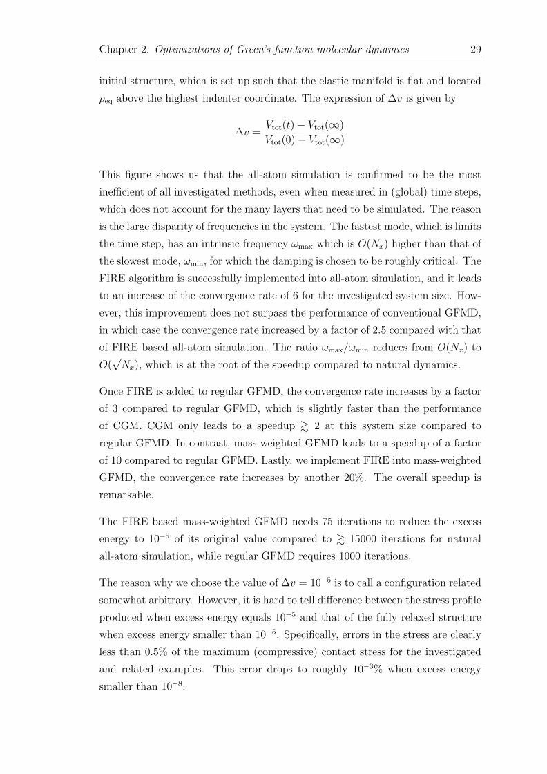
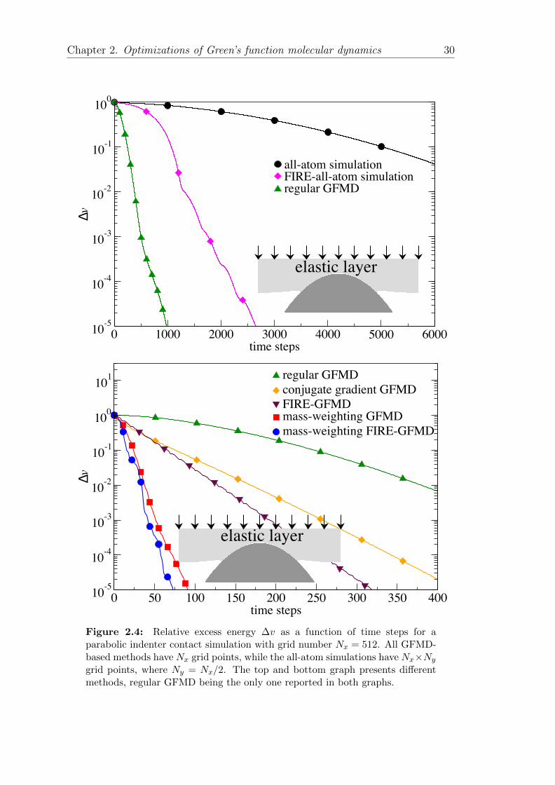
Fig 24 shows us how quickly various solution strategies minimize the energy at a
fixed system size Towards this end we first compute the excess energy ∆v which
is defined as the total potential energy minus the total potential energy of a fully
relaxed structure The excess energy is then divided by the value obtained for the
Chapter 2 Optimizations of Greenrsquos function molecular dynamics 29
initial structure which is set up such that the elastic manifold is flat and located
ρeq above the highest indenter coordinate The expression of ∆v is given by
∆v =Vtot(t)minus Vtot(infin)
Vtot(0)minus Vtot(infin)
This figure shows us that the all-atom simulation is confirmed to be the most
inefficient of all investigated methods even when measured in (global) time steps
which does not account for the many layers that need to be simulated The reason
is the large disparity of frequencies in the system The fastest mode which is limits
the time step has an intrinsic frequency ωmax which is O(Nx) higher than that of
the slowest mode ωmin for which the damping is chosen to be roughly critical The
FIRE algorithm is successfully implemented into all-atom simulation and it leads
to an increase of the convergence rate of 6 for the investigated system size How-
ever this improvement does not surpass the performance of conventional GFMD
in which case the convergence rate increased by a factor of 25 compared with that
of FIRE based all-atom simulation The ratio ωmaxωmin reduces from O(Nx) to
O(radicNx) which is at the root of the speedup compared to natural dynamics
Once FIRE is added to regular GFMD the convergence rate increases by a factor
of 3 compared to regular GFMD which is slightly faster than the performance
of CGM CGM only leads to a speedup amp 2 at this system size compared to
regular GFMD In contrast mass-weighted GFMD leads to a speedup of a factor
of 10 compared to regular GFMD Lastly we implement FIRE into mass-weighted
GFMD the convergence rate increases by another 20 The overall speedup is
remarkable
The FIRE based mass-weighted GFMD needs 75 iterations to reduce the excess
energy to 10minus5 of its original value compared to amp 15000 iterations for natural
all-atom simulation while regular GFMD requires 1000 iterations
The reason why we choose the value of ∆v = 10minus5 is to call a configuration related
somewhat arbitrary However it is hard to tell difference between the stress profile
produced when excess energy equals 10minus5 and that of the fully relaxed structure
when excess energy smaller than 10minus5 Specifically errors in the stress are clearly
less than 05 of the maximum (compressive) contact stress for the investigated
and related examples This error drops to roughly 10minus3 when excess energy
smaller than 10minus8
Chapter 2 Optimizations of Greenrsquos function molecular dynamics 30
0 1000 2000 3000 4000 5000 6000time steps
10-5
10-4
10-3
10-2
10-1
100
∆v
all-atom simulationFIRE-all-atom simulationregular GFMD
elastic layer
0 50 100 150 200 250 300 350 400time steps
10-5
10-4
10-3
10-2
10-1
100
101
∆v
regular GFMDconjugate gradient GFMDFIRE-GFMDmass-weighting GFMDmass-weighting FIRE-GFMD
elastic layer
Figure 24 Relative excess energy ∆v as a function of time steps for aparabolic indenter contact simulation with grid number Nx = 512 All GFMD-based methods have Nx grid points while the all-atom simulations have NxtimesNy
grid points where Ny = Nx2 The top and bottom graph presents differentmethods regular GFMD being the only one reported in both graphs
Chapter 2 Optimizations of Greenrsquos function molecular dynamics 31
So far we have anaylsed the performance of each algorithm with a fixed number of
discretization points in contact mechanics problem However it is often important
to know how the convergence rate scales with number of discretization points or
system size The related results are depicted in Fig 25
64 128 256 512 1024 2048Nx
102
103
num
ber
of i
tera
tio
ns
~Nx
038
~Nx
0
~Nx
025
~Nx
05
~Nx
10
~Nx
0
~Nx
085
~Nx
038
conjugate gradient GFMDFIRE GFMDmass-weighting GFMDmass-weighting FIRE-GFMD
102
103
104
105
106
nu
mb
er o
f it
erat
ion
s all-atom simulationFIRE-all-atom simulationregular GFMDconjugate gradient GFMD
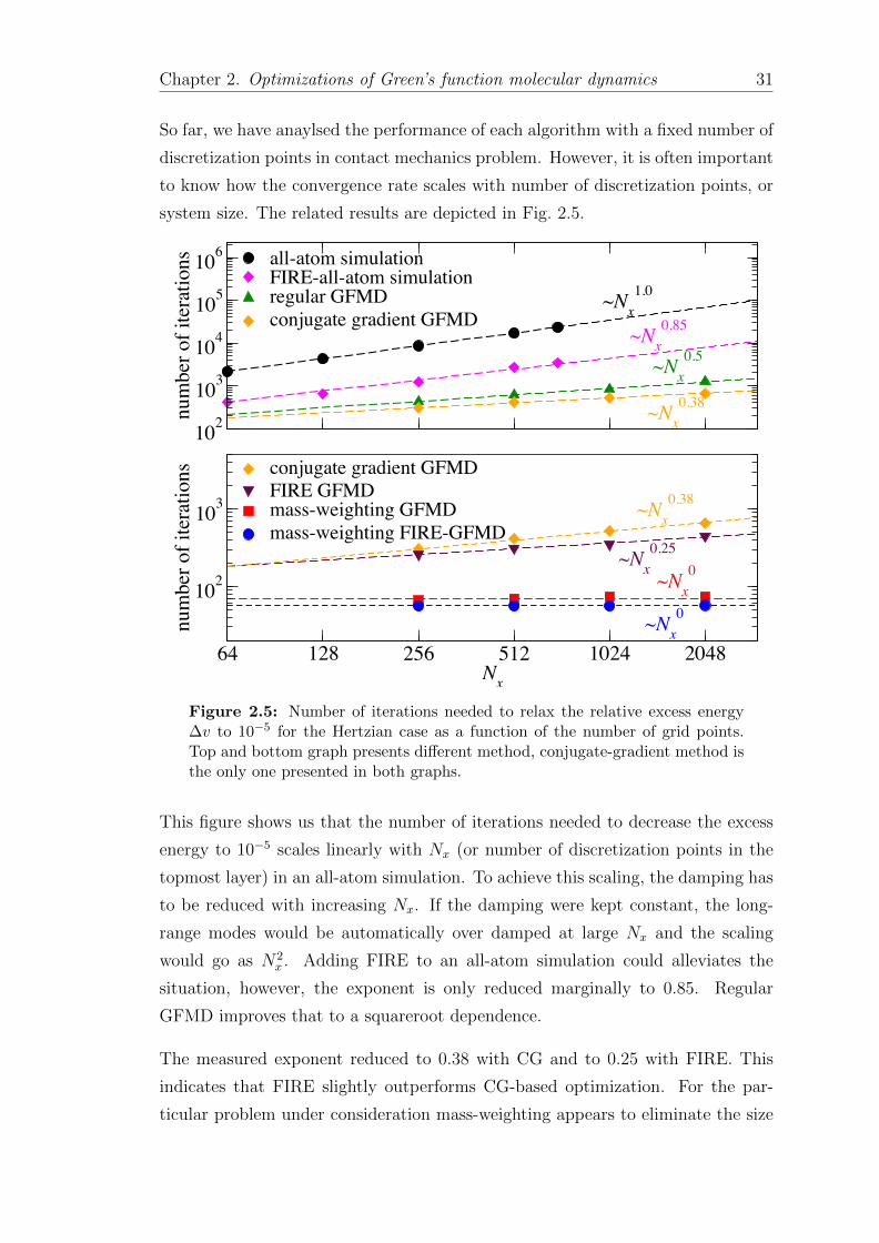
Figure 25 Number of iterations needed to relax the relative excess energy∆v to 10minus5 for the Hertzian case as a function of the number of grid pointsTop and bottom graph presents different method conjugate-gradient method isthe only one presented in both graphs
This figure shows us that the number of iterations needed to decrease the excess
energy to 10minus5 scales linearly with Nx (or number of discretization points in the
topmost layer) in an all-atom simulation To achieve this scaling the damping has
to be reduced with increasing Nx If the damping were kept constant the long-
range modes would be automatically over damped at large Nx and the scaling
would go as N2x Adding FIRE to an all-atom simulation could alleviates the
situation however the exponent is only reduced marginally to 085 Regular
GFMD improves that to a squareroot dependence
The measured exponent reduced to 038 with CG and to 025 with FIRE This
indicates that FIRE slightly outperforms CG-based optimization For the par-
ticular problem under consideration mass-weighting appears to eliminate the size
Chapter 2 Optimizations of Greenrsquos function molecular dynamics 32
dependence altogether
The scaling show in Fig 25 is found to be also valid for (2+1)-dimensional contact
problems whenever tested eg GFMD FIRE-GFMD and MW-GFMD When
the short-range repulsion was replaced by nonoverlap constraint the scaling was
also found to exist
In computer simulations considering the cost- and time-efficient issues it is also
significant to evaluate the relation between the CPU time per iteration and system
size which is analyzed in Fig 26 In all-atom simulations the relation between
CPU time per iteration and system size satisfies a scaling law with exponent
20 (30 for three-dimensional systems) However the exponent of this scaling
decreased to 10 (20 for three-dimensional systems) plus a logarithmic correction
for GFMD based approaches
In a typical simulation we could start with a relatively small system size for
which crude results can be obtained and reasonable parameters required for FIRE
damping or mass-weighting can be gauged After that the continuum limit can be
approximated with increasing resolution by keeping those parameters unchanged
In this way the number of iterations is much reduced
232 Randomly rough indenter
In this section the adhesive Hertzian indenter is replaced by a purely repulsive
self-affine rigid indenter Nevertheless the trends in results part remain similar
as depicted in Fig 27 Both FIRE and mass-weighting GFMD perform faster than
regular GFMD Implementing FIRE into mass-weighted GFMD the convergence
rate increased by a factor of 2 while the factor was 025 for simple parabolic
indenter contact case
233 Application to the contact-mechanics challenge
In this section we reinvestigate the contact-mechanics-challenge problem FIRE
algorithm is used to optimize the simulation Since this study is the first time for
us to implement CGM into GFMD it is possible to be unsufficient to conclude that
FIRE outperforms CGM The risk to be erroneous motivated us to apply FIRE
Chapter 2 Optimizations of Greenrsquos function molecular dynamics 33
100
101
102
103
Nx
10-7
10-6
10-5
10-4
10-3
10-2
10-1
100
CP
U t
ime
in s
econ
ds
iter
atio
nall-atom simulationconjugate gradient GFMDmass-weighting FIRE-GFMDregular GFMD ~N
x
2
~Nx(lnN
x+α)
Figure 26 CPU time in seconds per iteration as a function of the linearsystem size Nx The solid lines reflect fits while the dashed lines are reverseextension of the fits Adding mass weighting or FIRE or conjugate gradientmethod does not significantly affect the time per iteration for typically usednumbers All computations were performed on a laptop with a 16 GHz IntelCore i5 central processor unit (CPU) The FFTW version 335 is used in ourcode
GFMD to the problem defined in the contact-mechanics challenge CG methods
was reported to spend 3000 iterations for a discretization points of 32768times 32768
which definitely outrun the regular GFMD in terms of convergence rate for which
30 000 iterations were required to obtain a similar accuracy at that size The data
obtained from CGM which was submitted by Bugnicourt and coworkers revealed
convergence to a few 10minus9 times the maximum compressive stress An even greater
accuracy would certainly require higher data precision than those obtained when
requesting ldquodoublerdquo in C++ or ldquodouble precisionrdquo in Fortran
The convergence of FIRE GFMD for the contact-mechanics-challenge problem
is similar to that identified in this study for related contact problems FIRE
GFMD needs a little more than 500 iterations to reduce the excess energy to
10minus3 of its original value This value is slightly higher than that reported in the
previous benchmark which needs only roughly 300 to achieve the same reduction
Chapter 2 Optimizations of Greenrsquos function molecular dynamics 34
0 400 800 1200 1600 2000 2400time steps
10-5
10-4
10-3
10-2
10-1
100
∆vregular GFMDFIRE-GFMDmass-weighting GFMDmass-weighting FIRE-GFMD
elastic layer
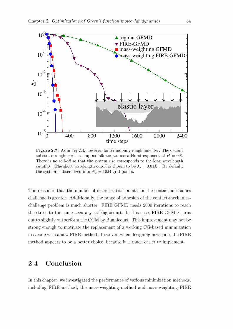
Figure 27 As in Fig24 however for a randomly rough indenter The defaultsubstrate roughness is set up as follows we use a Hurst exponent of H = 08There is no roll-off so that the system size corresponds to the long wavelengthcutoff λl The short wavelength cutoff is chosen to be λs = 001Lx By defaultthe system is discretized into Nx = 1024 grid points
The reason is that the number of discretization points for the contact mechanics
challenge is greater Additionally the range of adhesion of the contact-mechanics-
challenge problem is much shorter FIRE GFMD needs 2000 iterations to reach
the stress to the same accuracy as Bugnicourt In this case FIRE GFMD turns
out to slightly outperform the CGM by Bugnicourt This improvement may not be
strong enough to motivate the replacement of a working CG-based minimization
in a code with a new FIRE method However when designing new code the FIRE
method appears to be a better choice because it is much easier to implement
24 Conclusion
In this chapter we investigated the performance of various minimization methods
including FIRE method the mass-weighting method and mass-weighting FIRE
Chapter 2 Optimizations of Greenrsquos function molecular dynamics 35
method on classical BVPs within the framework of GFMD Two contact mechan-
ics problems were conducted as benchmarks to illustrate the extension of FIRE
In regular GFMD a critical damped dynamics for each surface Fourier mode
was set up to minimize the total potential energy It allows for the possibility
of short-range adhesion and even shorter-range repulsion and nonoverlap con-
straints Since GFMD is a MD technique introducing FIRE to GFMD would not
require much effort
It is demonstrated that FIRE can successfully accelerate a regular GFMD sim-
ulation resulting in a remarkable speedup of one order of magnitude for typical
system sizes compared to regular GFMD and even larger speedups for larger sys-
tems It is also possible to combine FIRE with other minimization methods in a
straightforward fashion in the framework of GFMD such as an effective choice for
the inertia of each mode This is known as a mass-weighting method which in-
duces a narrow distribution of intrinsic frequencies whereby the number of required
sweeps to relax the system no longer increases substantially with system size Even
though the relative speedup due to FIRE in such mass-weighted GFMD approach
is not overwhelming a factor of two in efficiency can still be useful for pushing the
boundaries of large-scale problems on massive parallel supercomputers
The successful implementation also indicates that the FIRE algorithm could also
benefit finite-element method or generally any engineering simulation that could
result in the solution of boundary value problems Experience from atomic-scale
applications shows that FIRE is always competitive with much more complex
mathematical optimization algorithms [47 82 83] (such as quasi-Newton methods)
and sometimes FIRE can even be superior [84]
Chapter 3
Thermal Hertzian contact
mechanics
This chapter attempts to study how thermal fluctuations affect the mean force
F (per unit area) between surfaces as a function of their interfacial separation
or gap g Furthermore it is also interesting to study if this relation could be
applied to classical Hertzian contact theory Towards this end we attempt to
construct the effective surface interactions Because a hard-wall constraint is the
most commonly used interaction between surfaces we restrict our attention to
the effect of thermal fluctuations on hard-wall constraints Since atoms fluctuate
about their equilibrium sites in solids thermal fluctuations automatically make
repulsion effectively adopt a finite range
The purpose of this chapter is to quantify thermal effects namely the relation
between the interfacial separation and the mean force obtained for flat walls Af-
ter that an extension of this relation to a Hertzian contact would be conducted
to ascertain its applicability Another purpose of this chapter is to identify an
analytical expression for the thermal corrections to the load-displacement relation
in a Hertzian contact
In the remaining part of this chapter the contact problem and the interaction
between surfaces are designed in Sec 51 The numerical technique is introduced
in Sec 32 while the theory is outlined in Sec 33 Numerical and theoretical
results are presented in Sec 34 and conclusions are drawn in the final Sec 54
37
Chapter 3 Thermal Hertzian contact mechanics 38
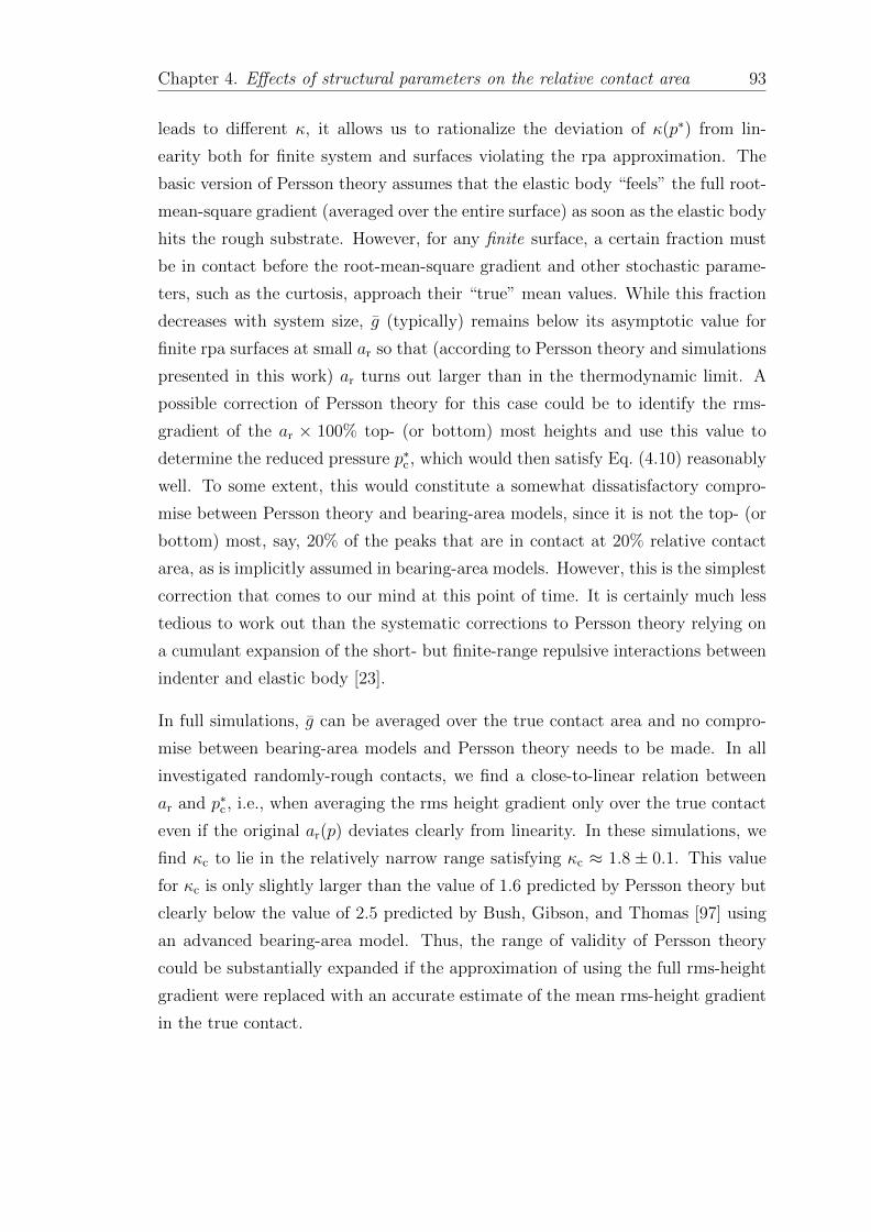
31 Model design
311 Treatment of elasticity and thermal displacement
In this study the elastic body is designed as initially flat semi-infinite and linearly
elastic The rigid substrate is fixed in space and the elastic body is moving from
above while the contact is defined as friction- and adhesionless The indenter as
designed in this study is either perfectly flat ie h(r) = 0 or parabola in which
case h(r) = minusr2(2Rc) where Rc is the radius of curvature In order to reduce
finite-size effects and to simplify both analytical and numerical treatments peri-
odic boundary conditions are assumed by default within the quadratic interfacial
plane
The elastic surface is subjected not only to an external load per particle l squeez-
ing it down against the indenter but also to thermal fluctuations as they would
occur in thermal equilibrium at a finite temperature T Additionally the small
slope approximation is applied to the counterface therefore the shear displace-
ment could be neglected
In this case the elastic energy of the deformed solid (semi-infinite thickness) can
be expressed as
Uela[u(r)] =ElowastA
4
sum
q
q |u(q)|2 (31)
Here u(r) states the z-coordinate of the elastic solidrsquos bottom surface as a function
of the in-plane coordinate r = (x y) Elowast is the contact modulus A the (projected)
interfacial area q an in-plane wave vector and q its magnitude
u(q) =1
A
intd2r eminusiqmiddotru(r) (32)
denotes the Fourier transform of u(r) The short-hand notation u0 = u(q = 0)
will be used for the center-of-mass coordinate
For a flat indenter only u0 will be used to denote the mean distance or gap
between indenter and the solid surface Here we define the displacement d as a
function of temperature and load according to
d(T L) equiv hind(r = 0)minus 〈u(T L r rarrinfin)〉 (33)
Chapter 3 Thermal Hertzian contact mechanics 39
where 〈u(T L r rarrinfin)〉 is the thermal expectation value that the field u(r) would
have (infinitely) far away from the top if the simulation cell were infinitely large
In this chapter we are interested mostly in the temperature-induced reductions of
d ie in the term dT defined in the expression
d = d0 minus dT (34)
where d0 indicates the displacement for an athermal Hertzian indenter at a given
load We compute dT through the following approximation
dT asymp 〈u(T L rX)〉 minus u(0 L rX) (35)
where rX is the most distant point from the center of the Hertzian indenter
312 Treatment of interaction
As in the reminder of this thesis the interaction is fully defined by the integral of
the surface energy density γ(g) over the surface which is a function of the local
interfacial separation or gap g(r) = u(r)minus h(r) between the surfaces It reads
Uint =
int
A
d2r γg(r) (36)
If the elastic energy is given explicitly the probability of a certain configuration
to occur would be proportional to the Boltzmann factor ie
Pr[u(r)] prop eminusβ(Uela+Uint) (37)
where β = 1kBT is the inverse thermal energy
This section will introduce a variety of interaction strategies that will be used in
this chapter
Chapter 3 Thermal Hertzian contact mechanics 40
Non-overlap constraint
The non-overlap constraint or hard-wall constraint is applied for most traditional
contact problems in which case the surface energy density is defined as
γ(g) =
infin if g lt 0
0 else (38)
This function indicates that the rigid indenter is not allowed to penetrate the
elastic sheet
In this study we will repeatedly go back and forth between continuous and discrete
descriptions of displacement fields For the discrete description the elastic solid is
split into individual atoms which are arranged on a square lattice with the lattice
constant ∆a Transitions between these two representations in real space can be
achieved with the substitutions
sum
n
harr 1
∆a2
int
A
d2r (39)
while transitions between summations and integrals in the Fourier space can be
achieved with sum
q
harr A
(2π)2
intd2q (310)
To simplify the analytical evaluation of integrals the square Brillouin zone (BZ)
of the surface will be approximated with a circular domain In this case the upper
cutoff for q is chosen to be qmax =radic
4π∆a as to conserve the number of degrees
of freedom with respect to the original BZ
Effective hard-wall potentials
Non-overlap constraints can be applied in GFMD simulations if the thermal effect
is neglected The basic idea of this constraint is sketched as follows elastic sheet
is split into discrete atoms and pressed against the rigid sheet once the atoms
penetrate the rigid solid they go back onto the surface This scheme no longer
works at finite temperature in which case the thermal fluctuation is considered
It violates the fluctuation-dissipation theorem (FDT) because the damping that is
Chapter 3 Thermal Hertzian contact mechanics 41
effectively imposed by this algorithm is not compensated by a conjugate random
force
In order to apply non-overlap constraint when thermal fluctuations are considered
a controlled fashion to violate of the rigid sheet should be allowed The resulting
procedure in terms of surface energy density function is given as below
γ(g) =κoE
lowast∆a
n
(minusg∆a
)nΘ(minusg) (311)
where Θ is the Heavyside step function κo is the hard-wall stiffness and n is a
dimensionless parameter
Although this procedure allows the atom penetrate the rigid sheet it is designed to
eliminate the penetration as quickly as possible Towards this end good numbers
for the exponent n and the dimensionless hard-wall stiffness κo need to be chosen
In order for the effective hard-wall potential to have a minimal effect on ∆t the
(non-negative) exponent n should be as small as possible However we would
like the force to be a continuous function for reasons explained at length in any
better text book on molecular dynamics [72 73] While these arguments can be
somewhat academic when the discontinuities are small we are going to send κo
to large numbers resulting in significant force discontinuities Thus n must be
chosen greater equal two This appears to make n = 2 the optimal choice
Regarding the choice of κo when ∆t and n are determined we should keep in mind
that we do not need extremely accurate dynamics in the rdquoforbiddenrdquo domain The
main purpose of this energy density function is to leave the rdquoforbiddenrdquo zone as
quickly as possible On the other hand the stiffness should be designed less than
a critical value above which the energy conservation is not satisfied for athermal
simulation even when Verlet algorithm is used For Verlet the critical time step
for a harmonic oscillator is ∆tc = Tπ where T is the oscillator period ie for
∆t lt ∆tc the trajectory may be inaccurate but the energy is conserved (except
for round-off errors) This can be achieved by setting the overlap stiffness to
ko = νo π2 m
dt2minus ks (312)
where ks = ∆u2(kBT ) while m is the inertia of the considered degree of freedom
νo is a numerical factor which must be chosen less than unity At and above the
critical value of νo = 1 energy conservation would be no longer obeyed in the
Chapter 3 Thermal Hertzian contact mechanics 42
absence of a thermostat At the same time dynamics but also static distribu-
tion functions are very inaccurate even if a thermostat prevents the system from
blowing up
The optimum value for ko certainly depends on the specific investigated problem
However the analysis of simple models can provide useful preliminary estimates
This will be done in Sec 312
Approximate collision rules
Another technique to apply hard-wall constraint with consideration of thermal
fluctuation is to use approximate collision rules and control the error of the im-
precision with the time step The implementation is summarized as follows ∆t
is fixed in simulation atom velocity changes sign if it violates the non-overlap
constraint The procedure in terms of pseudo code is sketched as follows in which
case the constraint is ignored
if (z violates constraint) then
z = 2zconstr-z
vz = -vz (velocity Verlet)
zold = 2zconstr-zold (standard Verlet)
end if
In a certain GFMD simulation in which case all observables are propagated in
Fourier space the following extra cost would have to be achieved not only the
current positions but also the old positions in real space will have to be stored
in memory for the purpose of the velocity calculation Additionally two extra
Fourier transforms on old positions will have to be requested which would double
the number of the most expensive function calls Since this approach appears to
show similar scaling with ∆t in simple models as effective hard-wall repulsion see
Sec 312 for more details we did not apply this procedure in this study in case
of time consuming
Chapter 3 Thermal Hertzian contact mechanics 43
Numerical case studies
To investigate the performance of these two approaches to mimic hard-wall con-
straint we study the following single harmonic oscillator problem thermal fluctu-
ations are applied to an originally free harmonic oscillator the resulting variance is
∆u2 Additionally this harmonic oscillator is then constrained to have no negative
deflections from its mechanical equilibrium site
Essentially the harmonic oscillator problem described above requires that kBT k
and m should be chosen such that the ∆u2 is unity (in units of kBTk) The default
time step that we use for the free oscillator is 2π30 ie 30 time steps per period
The damping coefficient is chosen to be γ = 1 whereby the free harmonic oscillator
is slightly under-damped Results for the convergence of how the estimate for the
mean displacement u0 approaches the exact value with decreasing time step ∆t
are shown in Fig 31
0 005 01 015 02 025 ∆t
05
06
07
08
09
u 0 ∆u
exactapproximate collision rulehard-wall potential
νο = 02
νο = 01
Figure 31 Mean displacement u0 in units of ∆u as a function of time stepsDifferent symbols represent different hard-wall approximation open circles in-dicates approximate collision rules and closed diamonds the harmonic effectivehard-wall potential Dash lines show linear fits while solid line shows the ana-lytical solution
Chapter 3 Thermal Hertzian contact mechanics 44
As shown in this figure the approximate collision rules turns out to be better than
the approximate hard-wall interactions at a given value of ∆t However u0 has
leading-order corrections of order ∆t in both approaches The error for effective
hard-wall potential is less than 1 with the choice of νo = 01 which is rigorous
for most simulations Additionally simulations must be conducted at two different
values of ∆t for the purpose of a meaningful extrapolation Considering that the
double times of Fourier transform when using approximate collision ruls would
result the time consuming problem we decided to apply the effective hard-wall
interaction for the full contact mechanics simulations
32 Thermal GFMD
GFMD is a boundary element method allowing us to effectively solve the elastic
response of a linearly elastic solid to boundary conditions [7 38 75] The elastic
surface displacement field is split into discrete atoms thus these atoms could reflect
the dynamic degrees of freedom Elastic interactions are applied on the surface in
terms of elastic Greenrsquos function In this study we consider a linear elastic solid
with semi-infinite thickness frictionlessly contacts with rigid counterface The
equation to be solved in GFMD is
mqumlu(q) + ηq ˙u(q) +
q Elowast
2u(q) = F (q t) (313)
where F (q t) is the Fourier transform of all external forces acting on the surface
atoms The terms mq and ηq represent inertia and damping coefficients of different
surface modes which may depend on the wave vector In this study we focus on
isotropic systems therefore both mq and ηq only depend on the magnitude q but
not on the direction of q
The thermal fluctuations can be explained as random forces which have to satisfy
the FDT [85] in which case the random forces must obey a zero mean and the
second moments must satisfy
〈Γ(q t)Γ(qprime tprime)〉 = 2 ηq kBT δqqprime δ(tminus tprime) (314)
Chapter 3 Thermal Hertzian contact mechanics 45
assuming discrete atoms finite domains but continuous times Here δ(bull) is the
Dirac delta function which can be replaced with δttprime∆t in a molecular dynamics
(MD) simulation in which the time t is discretized into steps of size ∆t
At this point GFMD is only used to generate the correct distribution of config-
urations whichmdashin a classical systemmdashdoes not depend on the choice of inertia
In this case the mq can be chosen at will as long as the stable configurations
can be reached In standard GFMD simulation mq is assumed to be constant
in which case identical simulations are obtained as if the Newtonrsquos equation were
propagated in real space However a realistic dynamics would be produced if
mq are chosen proportional to 1q In fact realistic dynamics require the treat-
ment of damping and random noise to have ldquomemoryrdquo as discussed in Ref [86]
When being interested in efficient dynamics which are useful to identify the local
minimum potential energy or stable equilibrium configuration quickly the mq are
better chosen proportionally to the stiffness at wave vector q which means small
value of mq for long-wavelength modes and large value of mq for short-wavelength
modes [75] In this context it is also worth mentioning that significant progress
has been made recently on GFMD to properly reflect not only true (rather than
efficient) dynamics of crystalline solids [87] but also for truly visco-elastic materials
with broad relaxation functions [41]
33 Theory
In this section we investigate the analytical expression for the thermal expectation
value of an interfacial force per atom f(u0) as a function of their mean separation
u0 in the case of hard-wall potential Towards this end a partition function
Z(N β u0) of a fluctuating surface in front of a wall is defined therefore the free
energy could be determined according to F(kBT u0) = minuskBT lnZ(β u0) The
mean force between hard wall and elastic surface can then be calculated from
f = minus 1
N
partF(N kBT u0)
partu0
(315)
Minor errors in the treatment presented below appear in numerical coefficients
that result for example by having approximated the Brillouin zone of a square
with a sphere or by having replaced a discrete set of wave vectors (finite system)
Chapter 3 Thermal Hertzian contact mechanics 46
with a continuous set (infinitely large system) However these and related ap-
proximations are controlled because errors resulting from them can be estimated
and they could even be corrected systematically
331 The statistical mechanics of a free surface
We start our theoretical study with the free surface which is the reference state
and the easiest case to investigate In this approach the variance of atomic dis-
placement caused by thermal fluctuation is an important quantity In the case of
fixed center-of-mass mode the variance is defined as
∆u2 equivlangu(r)minus u(0)2rang (316)
The variance could be computed in a straightforward fashion if we make Fourier
transform of the displacement which reads
∆u2 =sum
qprime
lang|u(qprime)|2
rang(317)
asymp A
(2π)2
intd2q
2 kBT
qElowastA(318)
asymp 2radicπ
kBT
Elowast∆a (319)
where we made use of equipartition for harmonic modes see also Eq (328)
The prefactor 2radicπ asymp 11284 turns out to be very close to unity However in a
quantitative theory we wish to know and perhaps to understand its precise value
Towards this end we assume the BZ to be square in real space with N atoms and
a summation based on this assumption is conducted It shows that ∆u2 can be
evaluated by
∆u2 =
(11222minus 124radic
N
)kBT
Elowast∆a (320)
ifradicN gt 512 to more than three digits accuracy This result is fairly close to the
analytical result based on a BZ which is approximated as sphere
Eq (319) reveals that the fluctuations are dominated by the small scales In
the case of an Einstein solid in which each surface atom is an independent har-
monic oscillator with identical stiffness kE = kBT(N minus 1) ∆u2 In reality ie
Chapter 3 Thermal Hertzian contact mechanics 47
in less than infinite dimensions there is always a correlation of thermal height
fluctuations
In this case the following question remains what is the distance over which height
fluctuations are correlated Towards this end we calculate the thermal displace-
ment autocorrelation function (ACF) Cuu(r) It can be defined and evaluated to
obey
Cuu(∆r) = 〈u(r)u(r + ∆r)〉 (321)
asymp 1
2π2
kBT
qElowast
int radic4π∆a
0
dq
int 2π
0
dϕ eiqr cosϕ (322)
=1
π
kBT
rqElowast
int radic4πr∆a
0
d(qr)J0(qr) (323)
=2 kBT
qElowast
radic4π r
∆a1F2
(1
2 1
3
2minusπ r2
∆a2
)(324)
asymp
2 kBTradicπ Elowast∆a
+O(r2) for r rarr 0
kBT(π q Elowast r) for r rarrinfin
(325)
in this expression J0(x) represents the Bessel function of the first kind and
1F2() a generalized hypergeometric function The analytical result of ACF shows
Helmholtz ringing at intermediate values of r This leads to the theoretical solu-
tion of little practical use except in the two limiting cases r rarr 0 and r rarr infin
Generally Helmholtz ringing is the result of feature such as abrupt cutoffs in the
wave vector domain However even using exact expectation values of |u(q)|2 for
a square BZ and extending the ACF to continuous limit between the lattice posi-
tions the Helmholtz ringing remains The validity of these claims is demonstrated
in Fig 32
One could generalize the Cuu(r) to a continuous function by constructing the
simplest expression with the correct limit behaviors which reads
Cuu(r) asymp2radicπ
kBT
Elowast1
(∆a2 + 4π r2)12 (326)
As shown in Fig 32 this asymptotic function is acceptable at a intermediate
domain where r = ∆a and the errors remain less than 5 in the limit of large
N for larger r Although numerical results presented in Fig 32 include data for
r parallel to [1 0] it is demonstrated that other direction such as [1 1] direction
could also get similar results
Chapter 3 Thermal Hertzian contact mechanics 48
Zhou et al Thermal contact mechanics
10-1 100 101 102
r Δa
10-3
10-2
10-1
100Cuu
(r)
Cuu
(0)
asymptotic approximationexact with interpolationnx = ny = 2048nx = ny = 512nx = ny = 128
Figure 2 The radial displacement ACF Cuu(r)mdashnormalized to its value at r = 0mdashas a function ofdistance r asymptotic approximation given in Eq (27) (black line) exact correlation function along the[10] direction with interpolation between non-lattice sites (dashed brown line) numerically exact results forsystems of size 2048 2048 (red circles) 512 512 (green squares) and 128 128 (blue diamonds) Theywere also obtained for the [10] direction except for the open symbols which refer to the [11] direction
A quite reasonable approximation or rather generalization of Cuu(r) to a continuous function can be made266by constructing the simplest expression with the correct asymptotic behaviors summarized in Eq (26)267
Cuu(r) 2p
kBT
E1
(a2 + 4 r2)12 (27)
As can be seen in Fig 2 this asymptotic approximation is quite reasonable already at a nearest-neighbor268spacing of r = a and has errors of less than 5 (in the limit of large N ) for larger values of r While269numerical results for finite systems in Fig 2 include predominantly data for r parallel to [1 0] similar270results are obtained for other directions as well as demonstrated examplarily for the [1 1] direction of the271N = 128 128 lattice272
The asymptotic ACF has decayed to approximately 30 of its maximum value at the nearest-neighbor273distance This means that the displacements of adjacent lattice sites are essentially uncorrelated274
The last property of interest used in the subsequent treatment is the partition function of a free surface275(fs)276
Zfs() =Y
q
qp2u2(q)
(28)
This is a provisional file not the final typeset article 10
Figure 32 The ACF Cuu(r)Cuu(0) as a function of r∆a Closed colorsymbols represent numerical results along the [10] direction for different systemsizes while open symbols refer to the numerical result along the [11] directionThe solid line represents the asymptotic approximation presented in Eq (326)while the dashed line the exact correlation function along the [10] direction withinterpolation between non-lattice sites
Another property should be noticed is that the asymptotic function has decayed
to roughly 30 of its maximum value at the nearest-neighbour distance This
indicates that the displacements of neighboring lattice sites are substantially un-
correlated
The partition function of a free surface is defined as
Zfs(β) =prod
q
λqradic2π∆u2(q)
(327)
with
∆u2(q) =2 kBT
q ElowastA (328)
λq = hradic
2mq kBT represents the thermal de Broglie wavelength of a surface
mode It indicates the ideal-gas contribution of the momenta conjugate to u(q)
to the partition function The intention of including λq into the calculation is to
Chapter 3 Thermal Hertzian contact mechanics 49
satisfy the partition function dimensionless as long as Elowast is small compared to
the external pressure and temperature kept fixed At this point a precise choice
of mq is not necessary even though it might be an interesting issue in itself
If the solid is simplified to an Einstein solid the partition function can be given
as
Zmf(β) =
(λmfradic
2π∆u2
)N (329)
where ∆u was sketeched above and λmf represents a mean-field de Broglie wave-
length
332 Interaction of a thermal elastic surface with a flat
wall
In this section the statistical mechanics of an initially flat linearly elastic surface
in front of a flat rigid wall is studied The purpose is to deduce the expression
of mean force in a straightforward fashion We conducted various mean-field ap-
proaches for this intention The theoretical results appears to be quite accurate
in different asymptotic limits of the full problem
First mean-field approximation
The Einstein solid which was introduced in Sec 331 is the most straightforward
way to thermal contact problem As a result a degree of freedom is a hybrid of
an atom in real space and a delocalized ideal sine wave Additionally we assume
that the elastic energy of an individual atom follows
vmfela(u) =
kBT
2 ∆u2u2 (330)
According to FDT the expectation value of u should remain zero towards this
end we assume that the interaction energy with a counterface placed at a distance
u0 from the atomrsquos mean position is given by
vmfsub(u) =
∆a2
2π
int 2π
0
dϕ γ(u0 + u cosϕ) (331)
This expression indicates that an oscillation of an atom leads to an undulation If
so u0 automatically corresponds to the atomrsquos mean position
Chapter 3 Thermal Hertzian contact mechanics 50
The excess free energy per particle ∆FN for a fixed center-of-mass position sat-
isfies
eminusβFN =1radic
2π∆u2
int infin
minusinfindu eminusβv
mfela(u)+vmf
sub(u) (332)
where the term ldquoexcessrdquo refers to the change of the free energy relative to that of a
free surface For hard-wall interactions the integral in Eq (332) can be evaluated
to be
eminusβFN =1radic
2π∆u2
int u0
minusu0du eminusβvela(u)
= erf
(u0radic2∆u
) (333)
Hence
FN kBT
= minus ln
erf
(u0radic2∆u
)(334)
asymp
minus ln
(radic2πu0∆u
)for u0 lt ∆u2
∆uradicπu0
eminusu20(2∆u2) for u0 gt 2∆u
(335)
The derivative of Eq (334) leads to the force expression from this first mean-field
approximation which reads
fmf1(u0) =
radic2
π
kBT
∆u
expminusu20(2∆u2)
erfu0(radic
2∆u) (336)
Second mean-field approximation
Another approach to thermal contact problem is to introduce an external force f
divided by the thermal energy instead of the interaction force such that u adopts
the desired value of u0 In this case the possibility of a displacement u to occur
reads
Pr(u) prop eminus(uminusu0)2(2∆u2)minusβf(uminusu0)Θ(u) (337)
where f should be well chosen such that 〈u〉 = u0 in which case the equilibrium
lattice position satisfies ueq = u0 + βf∆u2 In this case the restoring force in
the spring equals to zero The requirement 〈u〉 = u0 automatically leads to the
Chapter 3 Thermal Hertzian contact mechanics 51
following self-consistent equation for f
β f ∆u =
radic2
π
expminus (β f ∆u2minusu0)2
2∆u2
1minus erf(β f ∆u2minusu0radic
2 ∆u
) (338)
This approach leads to similar results for the f at small u0 as the first mean-
field estimation However the predicted force appears to be half that of the first
mean-field approach for large u0
Probabilistic approach
The third approach is to define the excess free energy of an elastic body in front
of a hard-wall by a path integral which reads
eminusβF(uprime0) =1
ZA
intD[u(r)] δ (uprime0 minus u0) eminusβ vtot[u(r)] (339)
where D[u(r)] denotes an integral over all possible displacement realizations and
ZA =
intD[u(r)] δ (u0 minus uprime0) eminusβ vela[u(r)] (340)
Eq (339) can be explained as follows the relative number of configurations that
are produced with the thermal equilibrium distribution of a free surface (fs) whose
maximum displacement is less than u0 ie
eminusβF(u0) = 〈Pr(umax lt u0)〉fs (341)
This interpretation motivated us to solve the following probability problem what
is the possibility of N prime = N∆a2∆Ac independent Gaussian random number satis-
fies 〈u〉 = 0 and ∆u2 lt u0 Here ∆Ac is the correlation area for the displacements
The distribution of umax = maxu(r) converges to the Gumbel distribution [88]
as long as the Gaussian random number N prime is large enough which reads
Pr(umax) =1
βgev
eminus(eminusz) (342)
with
z =umax minus microgev
βgev
(343)
Chapter 3 Thermal Hertzian contact mechanics 52
where microgev is the mode of the Gumbel distribution ie the most likely value for
umax to occur and βgev a parameter determining the shape of the distribution
For a normal Gaussian distribution ΦG(u∆u) they are given by
microgev
∆u=radic
2 erfminus1
(1minus 2
N prime
)(344)
βgev
∆u=
1
N prime middot ΦG(microgev∆u)(345)
in the limit of large N prime Here erfminus1() stands for the inverse function of the error
function [88]
As shown in Fig 33 the distribution of umax one time produced with GFMD and
another time by taking N prime independent random numbers are roughly identical
and both of them are almost dead-on the Gumbel distribution
30 40 50 60 70umax (kBTE∆a)12
00
05
10
15
20
Pr(u
max
) (k
BTE∆
a)1
2 128 5122048
nx = ny =
Figure 33 Distribution of maximum displacements for different system sizesClosed symbols represent the data obtained from GFMD simulation while opensymbols indicate the data obtained from N prime = 092N independent randomnumbers of mean zero and variance ∆u Solid lines represent the Gumbel dis-tributions
Chapter 3 Thermal Hertzian contact mechanics 53
Rather than relying on the Gumbel distribution one might as well write down
the exact probability of one positive Gaussian random variable (grv) to be less
than u0 and take the result into the N prime2-th power (On average there are N prime2
positive grvrsquos whose value may not exceed u0 The negative grvrsquos are irrelevant
with respect to the violation of the violation of the non-overlap constraint) In
this approximation
Pr(umax lt u0) =
erf
(u0radic2σ
)N prime2 (346)
and therefore
∆F = minusNprimekBT
2ln
erf
(u0radic2∆u
) (347)
This approach works for large separations in which case u0∆u 1 One should
notice that this expression is similar to the first mean-field case except for the
prefactor which is reduced by a factor of two while N is replaced with N prime
333 Thermal Hertzian contacts
Preliminary considerations
All variables needed to define a thermal Hertzian contact problem are listed as
follows the radius of curvature of the rigid indenter Rc grid distance ∆a contact
modulus Elowast external load L and thermal energy kBT Therefore the ther-
mal displacement dT should be identified by a function of variables listed above
Specifically at small temperature the leading-order approximation of the relative
displacement dTd0 can be expected to depend on powers of the variables declared
above which reads
dTd0
prop(Rc
∆a
)α(ElowastR2
c
L
)β (kBT
ElowastR3c
)γ (348)
where d0 represents the displacement of a typical athermal Hertzian indenter at
external load L Elowast and Rc are used to define the units of pressure and length
respectively Furthermore the exponents should satisfy the following rule which
is deduced with the help of dimensional analysis
α + 3β minus 5γ = 0 (349)
Chapter 3 Thermal Hertzian contact mechanics 54
The sum rule Eq (349) holds generally for temperature ranging from low to high
value
Low-temperature approximation
Low-temperature corresponds to weak thermal fluctuations in which case the
stress profile of a typical Hertzian contact problem is expected to be similar to
that of the athermal Hertzian contact problem except for a slightly deviation
This deviation then could be predicted as a constant shift dT according to the
perturbative assumption In this case the thermal Hertzian gap could be evalu-
ated with g(r) = gH(r) + dT where gH(r) is the Hertzian gap for athermal case
Considering that the dominant contribution to thermal energy are located in the
original contact domain the thermal energy per atom could be approximated as
eT = minusdT L+1
∆a2
intd2rFpa gH(r) + dT (350)
asymp minusdT L+2π
∆a2
int ac
0
dr rFpa(dT ) (351)
where Fpa equiv FN denotes the hard-wall free-energy normalized to the atom The
thermal displacement dT could be obtained by minimizing eT over T which leads
to
L =π a2
c
∆a2f(dT ) (352)
asymp π a2c
∆a2
radic2
π
kBT
∆u
exp (minusu202∆u2)
erf(u0radic
2∆u)(353)
where the last approximation is only valid at small temperatures Taylor expand-
ing this last expression leads todTd0
asymp T
T lowast(354)
with
T lowast =L∆a2
π kB Rc
(355)
High-temperature approximation
When the temperature is very high the thermal displacement dT is far beyond
the original displacement d0 so that the deformation of the elastic solid could
Chapter 3 Thermal Hertzian contact mechanics 55
be neglected In this case we assume the displacement field is a constant say
dT and the resulting individual forces can be summed up with a mean gap of
dT + r2n(2Rc) The external load then could be approximated as
L asymp N prime
2N
1
∆a2
intd2r fmf1
(dT +
r2
2Rc
)(356)
asymp L0∆u
dTeminusd
2T (2∆u2) (357)
with
L0 =
radic2
π
N prime
N
kBT Rc
∆a2 (358)
To solve Eq (357) we introduce Lambert W function W (x) asymp lnx minus ln lnx for
x 1 The thermal displacement in unit of ∆u could be evaluated as
dT∆uasympradicW
(L2
0
L2
) (359)
34 Results and analysis
341 Flat indenter
We have introduced three different theoretical approaches to the thermal contact
mechanics for a perfect flat-on-flat geometry in Sec 332 In this section we
explore for which case these approaches are consistent with the numerical results
obtained with thermal GFMD technique In numerical simulation we set contact
modulus Elowast = 1 grid distance ∆a = 1 and consider different values of u0∆u
As shown in Fig 34 the first mean-field theory is consistent with GFMD data for
small values of u0 while the probabilistic approach appears to be consistent with
GFMD data for large values of u0 There is a smooth transition between these
two limits which could be matched by the second mean-field theory However
as introduced in Sec 332 there is no closed form expression to describe this
transition On the other hand we noticed that these two limits have similar
functional form and the transition is quite continuous The limitation and property
mentioned above motivated us to apply a switching function to approximate this
transition as presented in Fig 34 this function matches the GFMD data ranging
from small to large values of u0 with maximum errors less than 10
Chapter 3 Thermal Hertzian contact mechanics 56
01 02 03 04 06 08 1 2 3 4u0 ∆u
10-4
10-3
10-2
10-1
100
101
β F
∆u
mean-field 1large-separation limitmean-field 2mean-field interpolation
64128
512 2048
nx = ny =
Figure 34 Dimensionless mean force βf∆u as a function of normalizedmean separation u0∆u where ∆u represents the height standard deviation ofa surface atom in the absence of a counterface
This switching function is given by
F(u0) asymp w1(u0)Fmf1(u0) + w2(u0)∆F (360)
with the weighting functions
w1(u0) =1
2
N prime
N+
(2minus N prime
N
)eminusu
20∆u
2
(361)
w2(u0) = eminusu20∆u
2 1minus tanh(u0∆u) (362)
where ∆F = minusN primekBT2 The negative derivative of Eq (360) with respect to u0
is nothing but the mean force f
Chapter 3 Thermal Hertzian contact mechanics 57
342 Hertzian indenter
So far an effective potential to describe the thermal effects in terms of repul-
sive force has been managed in a straightforward fashion In this section we
implement this potential into classical Hertzian contact problem to validate its
applicability Towards this end we investigate how thermal fluctuations effect the
load-displacement relation within the framework of GFMD Additionally the def-
inition of a contact area with consideration of thermal fluctuations is also studied
In order to avoid the discreteness problem the grid distance ∆a is set to sufficiently
small compared to the linear dimension of the contact area ac This convention
allows the simulation results to be consistent with the continuous Hertzian contact
theory
The default parameters to conduct the thermal Hertzian contact simulation are
listed as follows the radius of curvature Rc = 256 ∆a the normal load L =
131 Elowast∆a2 as a result contact area could be calculated with the area-load ex-
pression in classical Hertzian contact theory which is ac asymp 30 ∆a Results for
the displacement and stress profile at a given temperature kBT = 02Elowast∆a3 are
presented in Fig 35
When temperature is non-zero the boundary of contact and non-contact domain
becomes indistinct In this case the definition of ldquotrue contact areardquo should be
discussed explicitly In classical hard-wall constraint contact can be detected
only when elastic solids penetrate into rigid indenter is observed However when
thermal fluctuation is switched on the penetration behavior turns out to be in-
stantaneous and undetectable As a result the instantaneous contact area could
be argued to be zero However during each instantaneous time the forces between
surfaces is infinitely large consequently the stress profile is similar to a classical
Hertzian case after time averaging If the temperature is sufficiently small the
stress profile would very close to an athermal Hertzian case
Regarding the definition of true contact area we follow the idea that define a
contact line where the gradient of the normal stress has a maximum slope which
is proposed in a recent paper [89] In this example this definition leads to a
reduction of contact radius of order 1 while the normal displacement is reduced
by roughly 30
Chapter 3 Thermal Hertzian contact mechanics 58
-50 -40 -30 -20 -10 0 10 20 30 40 50r ∆a
000
002
004
006
008
σ (r
) E
hard-wall at kBT = 0
hard-wall at kBT = 02E∆a3
effective potential
-100 -50 0 50 100r ∆a
-50
-40
-30
-20
-10
00
10
20
u (r
) ∆
a
hard-wall at kBT = 0
hard-wall at kBT = 02E∆a3
effective potential
Figure 35 Top Interfacial stress σ as a function of distance r∆a fromthe symmetry axis The blue circles represent GFMD data at kBT = 0 withhard-wall overlap potential the blue line is the analytical solution of stress inHertzian contact problem The red open squares represent full simulation dataat finite temperature while the red dotted line shows GFMD data withoutthermal fluctuations however an effective potential was constructed to reflectthe thermal effects at a given temperature The arrow marks the point of largestslope for the thermal indenter Bottom Displacement field u(r) as a functionof distance r from the symmetry axis
Chapter 3 Thermal Hertzian contact mechanics 59
Unlike the definition of contact area the load-displacement relation for thermal
contact problem could be defined in a straightforward way As mentioned in
Sec 312 because of the repulsive force induced by the thermal fluctuations the
displacement d will reduced by dT The expression of displacement d for classi-
cal Hertzian contact problem is scale free in a similar manner the temperature
induced displacement dTd0 should also hold this property when ∆a ac As
shown in Fig 36 the thermal displacement dT for different Hertzian realizations
can be mapped exactly on a single master curve Ξ(TT ) which reads
dT = d0 Ξ(TT ) (363)
where
d0 =
(RcL
Elowast∆a3
)minus 13
d0 (364)
and
T =
(L
ElowastR2c
) 23 Elowast∆a3
kB (365)
The master curve describes the thermal displacement at low and high temperature
limits It shows that dT could be approximated with power laws however loga-
rithmic corrections should be made for both limits such that the approximation
could be consistent with GFMD data
Ξ(t) asympt (1minus ln t) for t 1
1727radict 1 + ln(t)6 for 01 lt t lt 104
(366)
Substituting the low-temperature limit to Eq (363) would result in the following
thermal displacement expression
dTd0
asymp T
T lowast
(1minus ln
T
T
)(367)
for T T This expression indicates that the low-temperature approximation
deduced in Sec 333 predicted correctly the linear term but failed to predict the
logarithmic corrections which become dominant for a small ratio TT
The argument that extending the integration domain in Eq (351) back to radii
beyond the athermal contact radius would lead better results at small TT is
demonstrated to be inefficient The reason is sketched as follows the displacement
Chapter 3 Thermal Hertzian contact mechanics 60
10-4 10-3 10-2 10-1 100 101 102 103 104
t
10-3
10-2
10-1
100
101
102
103
d T d
referenceL = 20 L (reference)Rc = 80 Rc (reference)AFMlarge-separation limit
~
t (1 - ln t)
1727 t12 1 + ln(t)6
Figure 36 Reduced thermal displacement dTd0 as a function of reducedtemperature t = TT for different Hertzian contact realizations The referencemodel (black circles) is defined in Sec 342 In one case load was increasedby a factor of two (red squares) and in another case the radius of curvaturewas increased by a factor of eight (orange diamonds) with respect to the defaultvalues Green triangles represent GFMD simulations with parameters in realunits ∆a = 25 A Rc = 200 nm Elowast = 100 GPa and L = 200 nN which wasa typical blunt atomic-force microscope (AFM) indenter contact Solid blueand red line show the low- and intermediate-temperature approximation fromEq (366) The dash line indicates the high temperature limit of Eq (359)
shift due to thermal fluctuations is assumed to be a constant which is inconsis-
tent with the results as shown in Fig 37 this shift far away from the indenter is
significantly larger than at r = 0 and this difference increases with decreasing tem-
perature Nevertheless we still decided to keep this low-temperature discussion
since it allows one to rationalize dT sim T relation to be linear
From a practical point of view one may want to study the thermal displace-
ments for real rather than for reduced units Before investigating this issue we
should make it clear that the range of application of the master curve presented
in Eq (366) for t gt 01 can only hold for the shown domain and cannot extend
to t rarr infin Nevertheless when t gt 103 the correlated temperature is already far
beyond that required for a typical real-laboratory experiment which turns out to
be almost impossible to be reached Therefore we would like to conclude that this
master curve is still applicable for practical purposes
Chapter 3 Thermal Hertzian contact mechanics 61
0 20 40 60 80 100 120 140 160 180r ∆a
0
1
2
3
4
5
6d T(r
) d
T( r =
0)
T T = 05 10-3
T T = 05
Figure 37 Spatially resolved thermal displacement dT as a function of dis-tance r∆a from the symmetry axis where dT was normalized to its value atr = 0 Dashed blue line represents the lower temperature case while solid redline represents the high temperature case
At this point we start to explore the issue that translating d(T ) dependence
with real units rather than reduced units Towards this end the expressions for
both low-temperature and intermediate-temperature limits are updated for a hard-
matter (Elowast = 1 GPa) and a soft-matter (Elowast = 50 MPa) system The expressions
are demonstrated by thermal GFMD simulations Results are presented in Fig 38
The radius of curvature was set to Rc = 50 nm for both cases and the external
load was adjusted so that plastic deformation can be neglected
Chapter 3 Thermal Hertzian contact mechanics 62
0 100 200 300 400 500 600 700T (K)
12
13
14
15
16
17
d (n
m)
low-temp expansion
E = 1 GPa Rc = 50 nmL = 20 nN ∆a = 025 nm
01 1 10163
164
165
intermediate-temperature expansion
0 100 200 300 400 500 600 700T (K)
-1
-05
0
05
1
15
2
d (n
m)
intermediate-temperature expansion
E = 50 MPa Rc = 50 nm L = 10 nN ∆a = 025 nm
Figure 38 Displacement d as a function of temperature T for fixed externalload Top figure corresponds to hard-matter (Elowast = 1 GPa) and the bottomfigure corresponds to soft-matter (Elowast = 50 MPa) Green circles indicate theGFMD data Red lines represent the intermediate-temperature approximationswhile blue dashed line represents the low-temperature approximation
Chapter 3 Thermal Hertzian contact mechanics 63
As shown in Fig 38 the GFMD results of both soft- and hard-matter match the
intermediate-temperature estimation at room temperature extremely well Rel-
ative corrections are required at low-temperature limit for hard-matter and can
be ignored for soft-matter This observation motivated us to explore the ques-
tion how far do thermal fluctuations affect the load-displacement relation This
question is critical to contact mechanics experiments because most indentation ex-
periments are conducted at constant temperature and varying load Substituting
the intermediate-temperature approximation of Eq (366) into Eqs (363ndash365)
and considering the displacement-load relation in classical Hertzian contact the-
ory leads to
dT = drefT
1minus 1
9ln(LLref
)(368)
with drefT asymp 1426 ∆u and
Lref =
(kBT
E∆a3
)32
ElowastR2c (369)
This expression indicates that when thermal fluctuation is switched on the thermal
shift is only roughly 15 times the thermal standard deviation of its smallest-scale
surface fluctuations
As shown in Fig 39 the thermal corrections leads to a constant shift for soft
matter systems When external load equals to L asymp 16 nN the corresponding
thermal shift is dT asymp 12 Reducing the external load by 100 times only leads to
a bare change of thermal shift say dT asymp 17 If twice the value of thermal dis-
placement compared to that at 16 nN is required a corresponding external load
of 20 fN is expected which is almost undetectable For reasons of completeness
we state that the range of validity of the intermediate-temperature approxima-
tion of 01 lt t lt 104 demonstrated in Fig 36 translates to a range of loads
of 015 lt LnN lt 15 middot 104 for the specific examples studied here This range is
sufficient for most of indenter experiments
35 Conclusion
In this chapter the effect of thermal fluctuations on classical Hertzian contact
mechanics in the case of hard-wall interactions is studied Towards this end we
Chapter 3 Thermal Hertzian contact mechanics 64
0 2 4 6 8 10 12 14 16 18L (nN)
-20
00
20
40
60
80
100
120
d (n
m)
Hertz theoryT = 0 KT = 300 K
E = 50 MPaRc = 50 nm
∆a = 025 nm
Figure 39 Displacement d as a function of external load L for a soft-matter(Elowast = 50 MPa) Blue circles indicate GFMD data with zero temperature andthe red circles indicate the GFMD data with T = 300 K which corresponds toroom temperature Black line is the load-displacement curve in Hertzian theoryRed dashed line represents the intermediate-temperature approximations
first investigate an initially flat elastic surface contacts with a flat rigid inden-
ter The purpose is to construct effective surface interactions so that the thermal
effect could be considered in the case of hard-wall interaction The thermal fluc-
tuations could be translated to a finite-range repulsive force The functional form
of this repulsive force was derived analytically and demonstrated to increase with
decreasing the interfacial separation u0 at small u0 but starts to decrease quickly
with increasing interfacial separation when u0 is sufficiently large
To validate the analytical approach Greenrsquos function molecular dynamics (GFMD)
technique was extended to include thermal fluctuations The most critical issue
that needs to be addressed here was how to deal with hard-wall interactions in the
simulations A stiff harmonic potential was introduced to replace the hard-wall
constraint and it turns out to be applicable if simulations are conducted at different
values for the stiffness and extrapolation is made to infinite stiffness The GFMD
Chapter 3 Thermal Hertzian contact mechanics 65
results are consistent with the different mean-field approaches to the thermal con-
tact mechanics problem addressed above In this way an accurate closed-form
displacement-force relation was obtained to describe the contact behavior of an
initially flat linear elastic solids and a flat rigid substrate
After that we applied this effective hard-wall interaction to the classical Hertzian
contact problem and a noticeable shift in the normal displacement is obtained
The thermal shift of Hertzian indenter was demonstrated to be slightly less than
15 times the thermal standard deviation of surface positions of a free initially flat
surface Logarithmic corrections which depend on external load turns out to be
negligible In this case thermal noise leads to a shift of the load-displacement curve
that is roughly equal to the root-mean-square fluctuation of surface atoms but
almost independent of the load Constant shifts usually hardly undetectable this
could potentially explain why Hertzian contact theory can be applied to nanoscale
problem without trouble
As expectation similar results should be reached if the classical Hertzian contact
replaced by randomly rough surface contact On the other hand if the short range
adhesion is included into this study we expect a reduction of this adhesion would
be obtained due to thermal fluctuations Future works could attempt to elucidate
this issue
Chapter 4
Effects of structural
parameters on the relative
contact area
This chapter attempts to understand what structural parameters characterizing
the surface topography affect the area-pressure relation in nominally flat contacts
Towards this end the friction- and adhesionless contact problem between an
initially flat linearly elastic solid and a rigid indenter with various profiles was
studied Specifically the indenter was designed to move from below and the
hard-wall constraint between these two bodies was imposed Greenrsquos function
molecular dynamics (GFMD) is a technique that allows us to solve this kind of
contact problem in the framework of MD which has already been widely used
in contact mechanics study [7 41 87 90] As throughout this thesis we use the
FIRE-GFMD which is demonstrated to be an efficient and reliable solver to locate
the stable mechanical structure of contact simulations quickly [75]
The first counterface investigated in this chapter is an isotropic randomly rough
indenter which is commonly used in many contact mechanics studies The second
case was also a randomly rough indenter however the isotropy was destroyed
The third case is an isotropic warping indenter which is a typical randomly rough
phase correlated surface The fourth and the last case was a generilized Hertzian
indenter
The remainder of this chapter is organized as followes The elastic body and
rigid indenter are introduced in Sec 41 The theory is sketched in Sec 42
which includes the construction of topographic order parameters beyond the Nayak
67
Chapter 4 Effects of structural parameters on the relative contact area 68
parameter Results are presented in Sec 43 while conclusions are shown in
Sec 44
41 Model design
411 Elastic body
The elastic body studied in this chapter is designed as initially flat linear elastic
body Periodic boundary conditions are assumed by default with the intention to
reduce finite-size effect and simplify the numerical simulation
An external load is applied to the elastic body so that the contact between elastic
body and rigid indenter could be measured In order to avoid one single point
contact the minimum load is adjusted to lead to at least one meso-scale asperity
in contact The interaction considered in this chapter is the hard-wall constraint
or non-overlap constraint in which case the contact is considered only if the pene-
tration of the elastic body is detected In addition the small-slope approximation
is also assumed which allows us to assume a zero shear-stress boundary conditions
between the bodies
412 Rigid indenter
Isotropic rpa indenter
The default indenter considered in this study is randomly rough self-affine surface
which is fully defined by a height power spectral function C(q) This kind of surface
has a feature that the stochastic properties are dominated by the resolution of the
measuring apparatus The spectrum used in this chapter reads
C(q) = C(qr)times
froll if q lt qr
(qqr)minus2(1+H) if qr lt q lt qs
0 else
(41)
where froll is a Boolean variable of which the value can only be zero or one It
is set to be zero by default in this study and only set to one when mentioned
Chapter 4 Effects of structural parameters on the relative contact area 69
explicitly In this case the roll-off wavelength λr = 2πqr plays the role of a long
wavelength cutoff Accordingly the properties of the isotropic rpa surface is fully
defined by the Hurst exponent H the system size L the roll-off wavelength λr
and cut-off λs = 2πqs and a prefactor C(qr) In practice L should be chosen
larger than λr to average implicitly over different random realizations which can
become relevant for large Hurst exponent at small relative contact area
The surface is defined according to
h(q) =radicC(q)e2πir(q) (42)
where r(q) is a uniform random number on (0 1) h(q) represents the Fourier
transform of height profile The real space representation could be obtained if the
following convention is applied
h(r) =sum
q
h(q)exp[iq middot r] (43)
h(q) =1
N
sum
r
h(r)exp[minusiq middot r] (44)
where N denotes the number of grid points into which the surface is discretized
Anisotropic rpa indenter
An anisotropic surface is realized by introducing a single number known as ldquoPeklenikrdquo
number γP The number results in an effective wavenumber
qP =
(γ2
Pq2x + q2
yγ2Pradic
γ4P + 1γ4
P
)12
(45)
as the variable to be used in the height spectrum rather than the true wave number
q The Peklenik number satisfies 0 lt γP ltinfin The isotropic rpa surface is realized
when γP = 1 The such produced height profiles reveal prefered directions or
ldquogroovesrdquo as shown in Fig 41
Chapter 4 Effects of structural parameters on the relative contact area 70
x L
yL h(r)σ
equilPos0dat u 12($3-avg)sig
0 02 04 06 08 1
0
02
04
06
08
1
-4
-3
-2
-1
0
1
2
3
4
10-3 10-2 10-1
∆r
10-4
10-3
10-2
10-1
100
G(∆
r)
σ h2
~∆r2
~∆r2H~∆r0
~∆r2
~∆r2H
approximation parallel to exapproximation parallel to ey
Figure 41 Top Anisotropic rpa surface profile with a Peklenik number ofγP = 4 Bottom Height-difference auto-correlation function C(r) for showntopography and r parallel to ex (closed black circles) and ey (closed pink circles)
Chapter 4 Effects of structural parameters on the relative contact area 71
Isotropic height-warped indenter
An isotropic height-warped surface is defined by
hw =
hmin + (hminus hmin)(
hminushmin
hmaxminushmin
)wif w ge 0
hmax minus (hmax minus h)(
hmaxminushhmaxminushmin
)|w|else
(46)
where hmin le Min h(r) and hmax ge Max h(r) Here h indicates the height
of an ideal randomly rough surface at a given position r and hw is the height
after warping transform at the same position According to this expression the
surface remains unchanged when w = 0 When w gt 0 peaks are blunted and
valleys are sharpened while the opposite is achieved with w lt 0 as can be seen
explicitly in the cross-section of the height profile shown in Fig 42 In the current
study hmin = 2Minh(r)minusMaxh(r) and hmax = 2Maxh(r)minusMinh(r) were
applied
Phase correlation through the warping procedure is reflected by the observation
that the height histograms are systematically skewed for w 6= 0 The reference
histogram is produced with rpa surface which turns out to be symmetric Ad-
ditionally the expectation value of the rms gradient is much increased in the
sharpened parts and significantly reduced in the blunted domains In contrast
for sufficiently large rpa surfaces g is independent of the height except near the
heighest and lowest heights in a finite sample In practical point of view the
Peklenik parameter should be correlated with wave vector [91] The warping sur-
face should also include additional refinements However our impression is that
the constant γP already includes the feature of scratched surface w = 2 could also
lead to a reasonable polished surface ie relatively deep valleys and smoothened
tops
Generalized Hertzian indenter
The last indenter is a generalized Hertzian indenter which is defined by
h(r) =R
n
( rR
)n(47)
where R is of unit of length r is the in-plane distance of a point from the symme-
try axis of an individual indenter which we place into the center-of-mass of the
Chapter 4 Effects of structural parameters on the relative contact area 72
-04 -02 0 02 04x L
-40
-30
-20
-10
00
10
20
30
40
h(x)
σ
w = 0
w = 2
w = -2
-4 -2 0 2 4 6h(r) σ
0
01
02
03
04
05
Pr[h
(r)σ
]
w = 0
w = 2w = -2
Figure 42 Top Height profile of warped indenters along a cross-section asa function of x coordinates Different color represents different warping w redfor w = 2 black for w = 0 and blue for w = minus2 The dashed lines indicate thecenter-of-mass height for the shown cross section The curves w = plusmn2 are shiftedby a constant to improve their visualization Bottom Height histograms forthe different surfaces
Chapter 4 Effects of structural parameters on the relative contact area 73
simulation cell Different values of n lead to different profiles In this study we
study the surfaces generated from three different values of n ie n = 15 (sharp
indenter) n = 2 (parabolic indenter) and n = 4 (blunt indenter)
42 Theory
421 Prediction of κ in Persson theory
Considering a linearly elastic solid in contact with an ideal randomly rough self-
affine fractal rigid substrate Persson theory predicts the area-load relation as
ar = erfradic
2 p0Elowastg (48)
where g is the rms height gradient averaged over the entire surface ie
g2 =
intd2q C(q) q2 (49)
Eq (48) not only works for randomly rough indenter but also holds for smooth
indenters with harmonic height profiles defined in Eq (47) if g is evaluated over
the true contact domains [92] in which case the g is replaced by gc Therefore the
range of applicability of Eq (48) appears to extend when re-expressing it through
ar = erf(radic
πκcplowastc2) (410)
where κc is the proportionality coefficient of area-load relation plowastc = p0(Elowastgc) rep-
resents the reduced pressure the index ldquocrdquo indicates that the quantity is evaluated
over the true contact zones rather than the entire surface
In fact when taking Persson theory literally it does ask the question how the rms-
height changes in a given point of contact (described using a small resolution of the
surface topography) when short-wavelength roughness is added to the description
of the contact problem Using the full spectrum to estimate this increase in the
rms-roughness can be seen as an approximation which might be possible to correct
in future work
Chapter 4 Effects of structural parameters on the relative contact area 74
Persson theory predicts a value of κ =radic
8π asymp 1596 In the formulation of the
theory it appears to us as if no distinction is made ndash or must be made ndash between
κ and κc at least as long as pressures lie in a range in which ar prop p that is if
p is sufficiently large for contact to spread out over clearly disconnected contact
patches but still small enough so that ar is less than say 005 Careful simulations
of sufficiently large systems find a relatively weak dependence of κ on the Hurst
roughness exponent eg κ(H asymp 08) 2 and κ(H asymp 03) amp 2 [35 52ndash54 57 93]
Analytical results for the Hertz contact result in κc asymp 1666 see also Eq (429)
and the more detailed discussion of periodically repeated smooth indenters in
Sec 435
422 Definitions of scalar parameters
Relative contact area is determined by the ratio of the true contact area and the
nominal contact area Therefore it is a scalar and it can only be a function of
other scalars such as reduced pressure plowast Nayak parameter ΦN and other scalar
structural parameters In principle structural parameters including Nayak pa-
rameter must follow the law of dimensional analysis some details about such
dimensional analysis could be found in Ref[40] Additionally real contact is de-
stroyed predominantly due to roughness at small wavelengths Therefore those
structural parameters Φi where i indicates an integer should not depend on pa-
rameters that are defined exclusively by parameters from the height-distribution
Because the structural parameters are closely correlated with square-gradient
height we could discuss the square-gradient term firstly When determining g
over a periodically repeated surface g2 equiv 〈(nablah)2〉 is identical to minus〈δh∆h〉 where
δh = h minus 〈h〉 and 〈bull〉 represents ensemble average However this equality only
holds for full contact If the situation from full contact turns to partial contact
we define
(gprimec)2
= minus〈δh∆h〉c (411)
the dependence of arel on parameters depending on height profiles in the contact
then becomes
arel = arel[p(Elowastgc) gcg
primec Φc] (412)
Ultimately arel is a functional of the height topography As such there should exist
a dependence of arel that does not necessitate parameters averaged over the real
Chapter 4 Effects of structural parameters on the relative contact area 75
contact However those might necessitate very non-local terms or alternatively
high-order derivatives of h(r) The latter may not be well defined when the surface
profile or its (higher-order) derivatives are not well defined as is the case for
example for a conical indenter Thus the following discussion assumes surface
height profiles to be sufficiently smooth
Regarding the construction of relevant parameters used to determine the contact
area it is useful to keep in mind three symmetry relations First inversion (r rarrminusr) leaves the contact area unchanged This is why each derivative with respect
to a spatial coordinate must appear an even number of times in the construction
of an invariant Second each measure should be rotationally invariant and reduce
to a scalar This is automatically achieved when representing derivatives with
the Einstein summation convention which requires every index (enumerating an
in-plane coordinate) occurring twice in a product to be summed over To use it
effectively we use it jointly with the index notation in which case h2α indicates
the square-height gradient (nablah) middot (nablah) and hαα the Laplacian ∆h However g
will keep indicating the rms height gradientradic〈h2
α〉 Third the invariants may
not change on a rigid vertical translation of the surface h(r) rarr h(r) + h0 This
is why only δh = hminus 〈h〉 can appear in the invariants The lowest-order invariant
obeying these rules that we could identify are given by
Φ1 =〈δh h2
α〉radic〈h2
α〉 g2(413)
Φ2 =minus〈δh2 hαα〉2radic〈δh2〉 g2
(414)
Φ3 =minus〈δh2〉 〈hαα〉2radic〈δh2〉 g2
(415)
Before constructing the next parameters the allowed values for the parameter Φ1
to Φ3 will be discussed Φ1 and Φ2 are identical when averaged over a periodically
repeated surfaces (as can be seen again by integration in parts) but not when they
are determined over partial contact in which case the index ldquocrdquo would be added
The parameter Φ3 is identical zero for periodically repeated surfaces but not for
finite contacts since the mean curvature disappears for a periodically repeated
surface while the curvature must average to a positive number for partial contact
(assuming the elastic body indents the profile from below)
Chapter 4 Effects of structural parameters on the relative contact area 76
The values of Φ1 and Φ2 averaged over a single rpa surface may be finite However
averaging these means over various disorder realization will make them disappear
as any surface realization h(r) has the same probability (density) to occur minush(r)
Thus Φ1 and Φ2mdashas well as any other parameter in which the symbol h appears
an odd number of times as a factormdashshould be small when determined over a
single rpa surface realization in particular when the roll-off domain is sufficiently
large
When averaged over partial contact andor over surfaces violating the rpa Φ1 and
Φ2 may and usually do take finite values This is why we call them symmetry
allowed in Table 41 For the remaining parameters we will no longer state the
rationale for why terms are symmetry allowed or forbidden as all relevant argu-
ments have been mentioned or are contained in Sec 423 Table 41 summarizes
our conclusions on each parameter constructed in this work
Additional parameters in which numerator and denominator are second order in
the derivative but higher order in h can be constructed They will be considered
up to the lowest order needed beyond the rms-height gradient in which the param-
eters do not disappear in case of the random-phase approximation This includes
the parameters
Φ4 =〈δh2 h2
α〉〈δh2〉 g2
(416)
Φ5 =minus〈δh3 hαα〉3 〈δh2〉 g2
(417)
For rpa-surfaces Φ4 is automatically equal to unity and for all periodically re-
peated surfaces Φ4 = Φ5
Finally we consider parameters in which the order of the derivatives is increased
from two to four while the order in the height is kept as small as possible Three
of quite a few resulting (irreducible) possibilities are
Φ6 =1
g4
langδh2rang〈hααhββ〉 (418)
Φ7 =2
3 g4
langδh2 hααhββ
rang(419)
Φ8 =1
g4
langh2αh
2β
rangminus 3
langh2α
rang langh2β
rang+ 〈hαhβ〉2
(420)
Φ9 =2
g4
langhαhβ minus h2
γ δαβ2rang2 (421)
Chapter 4 Effects of structural parameters on the relative contact area 77
where δαβ is the Kronecker-delta symbol
The parameter Φ6 is nothing but the Nayak parameter ΦN up to a multiplicative
constant of 23 It is frequently interpreted as a measure for the spectral width
We chose the prefactor such that Φ6 and Φ7 are equal to unity for single-wave-
vector roughness The parameter Φ7 is a generalization of the Nayak parameter
For randomly rough rpa surface its expectation value is close to but less than Φ6
Thus both parameters tend to infinity as the ratio εf = λsλr becomes large that
is with εminus2Hf However for (strongly) correlated random roughness Φ7 takes much
greater values than Φ6 just as Φ4 starts to substantially exceed unity because the
factorization of the various terms (see also Sec 423) no longer holds once the rpa
is no longer satisfied
The parameter Φ8 plays the role of a generalized height gradient cumulant It is
constructed such that it takes the value of zero when the fourth-order cumulant
of the surface slope s parallel to any in-plane unit vector n takes the value of zero
if it is distributed normally ie when c4n = 〈s4〉 minus 3〈s2〉2 disappears for every n
This parameter is implicitly symmetrized with respect to its mirror images in the
xz and yz planes so that 〈s〉 = 0 follows Note that Φ8 being small is a necessary
but not a sufficient criterion for every c4n to disappear It is only sufficient if the
surfaces are stochastically isotropic
Finally Φ9 is a measure for anisotropy It takes the values of zero and one in the
limits of ideal isotropic and ideal anisotropy respectively where for the latter
surfaces are perfectly smooth along one spatial direction Assuming the Peklenik
number to be independent of the wavevector Φ9 can be easily shown to be identical
to (γ2P minus 1γ2
P)2(γ4P + 1γ4
P) As is the case for some other parameters too Φ9
is not identical to zero for an individual surface realization but only averages to
zero after taking sufficiently many surface realizations
We conclude this section by stating that the Nayak parameter is the lowest-order
scalar structural parameter that the proportionality coefficient κ can depend on if
the surface is isotropic and satisfies the random-phase approximation All other
parameters of similar or smaller order in height are either identical to zero or their
expectation value is zero or they strongly correlate with the Nayak parameter
Chapter 4 Effects of structural parameters on the relative contact area 78
full prs rpa n-rpaΦ1 ε allowedΦ2 Φ1 Φ1
Φ3 0 0Φ4 1minus ε allowedΦ5 Φ4 Φ4
Φ6 allowed allowedΦ7 asymp Φ6 allowedΦ8 ε allowedΦ9 ε ε
if isotropic if isotropic
Table 41 Values of parameters averaged over a full periodically repeatedsurface (prs) if the random-phase approximation (rpa) is valid and when it isnot valid (n-rpa) The word ldquoallowedrdquo indicates that a finite value is symmetryallowed The number ε implies that the result averages to zero after an ensem-ble average over many surface realizations and that it should be small for anindividual instantiation
423 Evaluation of fourth-order invariants
For (isotropic) randomly rough surfaces invariants being fourth order in height and
fourth order in derivatives are the leading-order scalar structural parameters that
can affect the proportionality coefficient κ Of particular interest should be those
thatmdashunlike the Nayak parametermdashcannot be reduced to products of invariants
being second order in height Yet the evaluation of fourth-order expressions is
commonly done using Wickrsquos theorem [94] which applied to the current problem
translates to
C4(q1 q4) equivlangh(q1)h(q2)h(q3)h(q4)
rang
asymplangh(q1)h(q2)
ranglangh(q3)h(q4)
rang
+langh(q1)h(q3)
ranglangh(q2)h(q4)
rang
+langh(q1)h(q4)
ranglangh(q2)h(q3)
rang (422)
whereby expectation values of fourth-order expressions are reduced to products of
height spectra since
langh(qm)h(qn)
rangprop C(|qm|) δ(qm + qn) (423)
Chapter 4 Effects of structural parameters on the relative contact area 79
where C(q) is the height spectrum Eq (422) is exact for Gaussian random
variables of mean zero
43 Results
431 On the accurate calculation of ar and κ
In a recent study proposed by Yastrebov and coworkers [61] a new expression
to estimate the relative contact area in purpose of ensuring an unprecedented
accuracy is given
ar =nc minus αncl
ntot
(424)
where ntot is the total number of points into which the surface is discretized and
α = (π minus 1 + ln 2)24 nc is the number of contact points ncl the number of
contact line points which are in contact but have at least one non-contact point
as nearest neighbor
For an isotropic rpa surface this expression turns out to be quite efficient to get
an applicable accurate relative contact area Nevertheless we believe that the
performance can at best be comparable with a properly executed Richardson ex-
trapolation The reason is that the numerical coefficient α asymp 011811 can hardly
be universal even if the special form of writing it as (πminus1+ ln 2)24 might convey
an intelligent mathematical reason for its specific value To make it clear let us
assume that the leading order correction were truly follow the idea of Eq( 424)
in which ar is proportional to the number of contact line points within the contact
domains This number would ultimately scale with aλs because the fractal na-
ture of the contact seizes exist in this limit so that the contact line acquires the
(fractal) dimension of unity This linear scaling of the leading order corrections
to the contact area would be picked up by Richardson extrapolation and the pro-
portionality coefficient would automatically adjust to the exact value and not to
a value which is very good but not exact
The proposed correction scheme can only outperform a Richardson extrapolation
if higher order corrections happened to be incorporated into it as is shown in
Fig 43 by the accurate values from the Yastrebov extrapolation at large εc How-
ever since the exact value α must depend on the specifics of a simulation it
Chapter 4 Effects of structural parameters on the relative contact area 80
can only be exact in isolated cases of measure zero so that it is generally asymp-
totically inferior to Richardson As such a claim of having provided data with
unprecedented accuracy with this method is not justified given that previous works
used a Richardson extrapolation while employing ratios of εc = aλs εf = λsλr
and εt = λrL which were simultaneously all greater than the data having the
purportedly unprecedented accuracy
00 01 02 03 04 05a λs
0100
0102
0104
0106
0108
0110
a r
Yastrebovmod YastrebovRichardsonGFMD data
Figure 43 Relative contact area ar as a function of aλs for an isotropicrpa surface with different extrapolation schemes The parameters to define thesystem are specified by H = 08 plowast = 005 λrL = 05 and λsL = 0008 Inthe modified Yastrevob extrapolation the prefactor α in Eq (424) was chosensuch that the extrapolated contact area remain unchanged if discretization aλs
increased by a factor of 2
To improve the performance of Yastrebovrsquos scheme an incorporation of Richardson
extrapolation could be applied Consider two independent contact simulations
with different values of aλs while leave other parameters identical For the two
simulations the Yastrebovrsquos extrapolation should lead to identical relative contact
area Therefore the resulting α should also be adjusted such that the extrapolation
could give the same estimation This modification leads to an improvement as
can be seen in Fig 43 However the performance turns out to be imprecise when
Chapter 4 Effects of structural parameters on the relative contact area 81
aλs ge 14 In our contact simulations including rpa surface and warped surface
we noted that the result produced from Yastrebovrsquos extrapolation with the choice
of α = 011 appears to be very close to that of Richardson extrapolation say
within 01 In order to apply Yastrebovrsquos extrapolation scheme in our study
without loss of precision we choose α = 011 and the discretization of aλs 14
This value of α typically deteriorates the quality of the contact area estimation
for a = λs2 but improves it overall otherwise
Lastly different pressures may lead to different errors in Yastrebovrsquos extrapolation
scheme In this case the following questions remain What is the origin of their
observed logarithmic correction of κ on pressure Is it the lack of a rigorous
extrapolation to the continuum (εc = aλs rarr 0) the fractal (εf = λsλr rarr 0)
the thermodynamic (εt = λrL rarr 0) limit Or is it actually true Even though
our comments of their self assessment are critical their data appears to be of
similar quality as that most other leading works which had all together come to
the conclusion that κ would remain unchanged at small p [42] but which either
simply took the values at the smallest value of εc without further extrapolation
or that made Richardson extrapolations which we can no longer reconstruct [54]
In a recent study managed by Nicola and coworkers [42] they show logarithmic
corrections in κ at small p for (1+1) dimensional contact simulations even for very
large sizes when many different meso-scale patches exist
To investigate if κ is constant or not at small pressure the trends of κ at limit
prarr 0 is studied Towards this end we compute κ as a pressure-dependent function
through the equation
ar = erf(radic
πκplowast2) (425)
rather than through arplowast because Eq (425) accounts for some of the low-pressure
non linearities as can be appreciated in Fig 1 of Ref ([95])
432 Isotropic rpa surfaces
Does κ have a low-pressure limit
κ cannot have a finite low-pressure limit if it is defined or computed according to
κ =
(prod
x
limεxrarr0
)limprarr0
κ(p) (426)
Chapter 4 Effects of structural parameters on the relative contact area 82
where the various limits (defined in the previous section with x taking the ldquovaluesrdquo
c for continuum f for fractal and t for thermodynamic) are taken in arbitrary
order The reason is that for any finite system if pressure is extremely small only
the highest asperity could be in contact which is similar to Hertzian contact in
which case κ results in infinity
Because it is not possible to get a finite limit with the definition of κ presented
above we turn to another approach to obtain the low-pressure limit which reads
κ = limprarr0
limεtfrarr0
ar
plowast (427)
With this definition we attempt to study whether ar can be proportional to p
over an extended range in pressure with no or negligible logarithmic corrections
to the proportionality coefficient κ if both εtf are sufficiently small while εc is
properly taken to zero at each pressure This limit is certainly not approached
if the product εtεf is not taken to infinite similarly small while having a varying
discretization errors as in Ref [61] Another approach proposed by Prodanov et
al [54] they managed to keep all but one εtfc constant However this idea is
not good enough because the discretization corrections probably decrease as εf
decreases due to the increase of the characteristic patch size Additionally they
assumed that the leading errors to κ follow the sum of the power law in terms of
εx while they could also be of a more general form
Alternatively to study the trend of κ at small pressure limit we ran simulations
in which εt andor εf were decreased simultaneously with decreasing pressure
according to
ε = εref (ppref)14 (428)
Results are shown in Fig 44 It reveals that κ increases apparently with decreasing
p for all three H = 03 cases while it essentially plateaus for the two H = 08
cases in which εf is decreased as p decreases If the pressure is further decreased
the H = 03 cases could eventually reach plateaus In this case a qualitative
difference between H = 03 and H = 08 would remain The curves for which εt
and εf are decreased with decreasing pressure lead to small values of κ for H = 08
but to large values for H = 03
The reason for this phenomenon could be potentially linked to the distribution
of contact patch areas and the characteristic contact patch size Ac which we
define to be the expected patch size that a randomly picked contact point belongs
Chapter 4 Effects of structural parameters on the relative contact area 83
005 01 02p
19
20
21
22
κ
H = 03 08
εt = const εf = varying
005 01 02p
19
20
21
22
κ
εt = varying εf = const
εt = varying εf = varying
Figure 44 κ as defined in Eq (427) as a function of reduced pressureplowast Different color represent different choice of how εft change with pressure pOpen and closed symbols represent H = 03 and H = 08 respectively The termldquoconstrdquo relates to εt = 12 and εf = 132 The reference value of pressure isplowast = 02 The term ldquovaryingrdquo indicates that the respective ε is scaled accordingto Eq (428)
to The three H = 03 curves and the H = 08 case with fixed εf all of which
belong to those simulations in which the characteristic contact areas are rather
small According to a recent study on contact patches [96] Ac increases only
logarithmically with εf for H lt 05 In this case large patches are not possible
to occur for H = 03 cases even when εf is small Additionally even for H = 08
case only small contact patches are allowed to arise at pressures well below the
percolation threshold if εf is fixed to a constant value as large as εf = 132
Conversely large contact patches can arise even at small pressures if εf is small
and H gt 05 The large patches play a significant role in the linear area-load
relation at small pressure as can be rationalized qualitatively from bearing-area
models
To investigate whether κ has a well-defined limit when being deduced with the
meaningful limit defined in Eq(427) we ran simulations with two sets of εtf to
Chapter 4 Effects of structural parameters on the relative contact area 84
comprare the resulting κ(p) relation the first case is a small system with εt = 1
and εf = 132 another case is a larger system with εt = 14 and εf = 1128
The results are depicted in Fig 45 This figure demonstrates that with increasing
system size ie decreasing εt and εf the pressure sensitivity of κ turns out to be
remarkable for H = 08 case but not for H = 03 case
The tendancies revealed in Fig 45 are consistent with those of Fig 44 ie
increasing system size leads to a reduction of κ and its pressure sensitivity for
H = 08 but not for H = 03 The trends also roughly match the observations by
Prodanov et al [54] who proposed the existence of a well-defined value of κ for
H = 08 but not for H = 03
So far we have already speculatively linked the different trends for H = 03 and
H = 08 to the way how a characteristic contact patch size changes with de-
creasing εf It motivated us to explore the explanation why Ac increases only
logarithmically with εf for H lt 05 but algebraically for H gt 05 One potential
reason could be that most of the elastic energy (in full contact) is stored in long-
wavelength modes for H gt 05 but in short-wavelength modes for H lt 05 If this
consideration were tenable H = 05 could be the dividing line for the divergence
We therefore repeated simulations for H = 05 case as shown in Fig 45 How-
ever the results leave us uncertain More rigorous works should be conducted to
characterize the transition between the different scaling behaviors in future
In this section we studied the trend of κ at zero pressure limit for an isotropic
rpa surface in a manner of Eq (427) For small Hurst exponent ie H lt 05
it might not exist andor it might depend on how εf rarr 0 is approached eg it
could take different valus when reaching it with constant εfεt and with constant
εfradicεt Meanwhile we expect that the value of κ =
radic2π asymp 25 predicted by the
BGT model [97] might provide a (potentially rigorous) upper bound for κ when
the limit εt rarr 0 is taken before εf rarr 0
Effect of Nayak and related parameters on κ
Yastrebov et al [61] came up with a decreased logarithmic dependence of κ on the
Nayak parameter for isotropic randomly rough self-affine surfaces However this
dependence appears to be problematic with respect to two aspects of their claim
and their data First κ is implicitly predicted to become negative for very large
Chapter 4 Effects of structural parameters on the relative contact area 85
10-3 10-2 10-1 100
p
16
18
20
22
24κ
10-3 10-2 10-1 100
p
16
18
20
22
24κ
10-3 10-2 10-1 100
p
16
18
20
22
24κ
εt = 1 εf = 132
εt = 14 εf = 1128H 03 05 08
0001 001εf
19
20
21
κ
p = 0005p = 005
Figure 45 Top κ as a function of reduced pressure plowast Different colorindicates different Hurst exponent Open symbols represent GFMD data withthe choice of εt = 1 and εf = 132 while closed symbols εt = 14 and εf =1128 Bottom Scaling with εf for H = 08 and εt = 05 Dashed lines arelinear fits to the three lowest values in εf Results were averaged over up to 100random realizations per data point
Chapter 4 Effects of structural parameters on the relative contact area 86
Nayak parameters which is physically meaningless Second their data points seem
to be partially inconsistent eg in their Fig10d the points (ΦN κ) = (700 193)
and (70 205) should be moved to (70 193) and (700 205) respectively In this
way the Nayak parameter ΦN would be consistent not only with our own cal-
culations but also with the values that Yastrebov et al reported themselves in
their Fig1 Once these two data points are corrected the logarithmic dependence
seems to be much less convincing than with improperly plotted data
The suspectable logarithmic dependence of κ on Nayak parameter motivated us
to run simulations to present an independent test of the extent with which the
Nayak parameter affects κ In our simulations we expand the range of surfaces
and contrast surfaces with cutoff to those with smooth and sharp rolloffs Results
are presented in Fig 46 which were averaged over up to 400 random realizations
per data points
As shown in Fig 46 the averaged values of κ turn out to be consistent with a
κ(ΦN) = κ(infin) minus cNΦminusνNN relation rather than a decreased logarithmic relation
Two different dependencies plotted in Fig 46 correspond to H = 03 and H = 08
case respectively Therefore κ cannot be concluded to be a single function of ΦN
(and plowast) at least not possible for different Hurst exponent
433 Anisotropic rpa surfaces
In this section we attempt to understand how anisotropy affects the relative con-
tact area Towards this end we repeated the simulations presented in Fig 44
with a Peklenik number of γP = 4 As shown in Fig 47 the pressure dependence
of κ at fixed value of εtf is improved compared the ideal rpa surfaces with γP = 1
This result may not be particularly surprising in consideration of the observation
that one-dimensional surfaces have logarithmic corrections to the κ(p) relation
even for H gt 05
Fig 47 also shows that κ is not very pressure sensitive for H = 08 when εf is
decreased with pressure so that for macroscopic systems in which εf is two or
three orders of magnitude smaller than in simulations the pressure sensitivity is
marginally small However compared with the isotropic case κ is apparently in-
creased due to anisotropy When the Peklenik number is chosen far from unity
different law may apply as the surfacersquos dimensionality has effectively changed
Chapter 4 Effects of structural parameters on the relative contact area 87
101 102 103 104
ΦN
19
20
21
κ
H = 08
H = 03
12
3
1
2 3
4
4
Figure 46 Proportionality coefficient κ as a function of the Nayak parameterΦN = 15 Φ6 at plowast = 002 Full and open symbols relate to H = 03 and H = 08respectively Different surface realizations were considered (1) orange trianglesup cut-off (2) blue triangles down smooth roll-off (3) green triangles lefthard roll-off In these three cases εt and εf were fixed εt = 14 εf = 1125Finally (4) squares cut-off with 140 le εf le 11000 The dashed lines are fitsκ = κinfin + cΦminusνN where ν turned out to be consistent with ν asymp 05 for H = 08and ν asymp 1 for H = 03
from two to one In a recent study on κ the tendency for one-dimensional con-
tact problem the pressure sensitivity of κ at the zero pressure limit has been
convincingly established not only for small H but also for H = 08 [42]
Additionally regarding the anisotropic rpa surfaces we noticed that κc whose
definition of reduced pressure uses the rms height gradient g averaged over the
contact domain only has a fairly weak dependence on plowast Values of κc are roughly
close to 18 Interestingly the order of the points are essentially in reverse order
compared to the analysis in which g was averaged over entire surfaces
Lastly as shown in Fig 47 the smallest κ occurs for the smallest Hurst exponent
The explanation could be as follows for H = 03 roughness exists mainly at small
wavelengths and as a result contact patches are rather small compared to H = 08
Chapter 4 Effects of structural parameters on the relative contact area 88
005 01 02p
16
18
20
22
24
26
28
30
κ
H = 03
εt = varying εf = const
εt = varying εf = varying
005 01 02p
16
18
20
22
24
26
28
30
κ
κc κcεt = const εf = varying
005 01 02p
16
18
20
22
24
26
28
30
κ
κ
005 01 02p
16
18
20
22
24
26
28
30
κ
κ
005 01 02p
16
18
20
22
24
26
28
30
κ
H = 08
Figure 47 The interpretation is similar to Fig 44 however the rigid inden-ter used in this figure is replaced by an anisotropic indenter with γP = 4 Thecolor symbols used in this figure which are not used in the Fig 44 representresults for κc
The coarse grained or rotationally averaged height profile of an individual meso-
scale asperity is therefore blunter for H = 08 than H = 03
434 Isotropic height-warped surfaces
Most of contact studies focus on the ideal rpa surfaces with assumption of the
random-phase approximation quite a few numerical studies use a Weierstrass pro-
file which has phase correlation while producing a height autocorrelation function
(ACF) being similar to experimental ACFs Nevertheless the Weierstrass profile
is far from those experimental surfaces as demonstrated in Fig2 of Ref [98] This
convinces us that the warping surface introduced in Sec 41 while perhaps far from
ideal reproduces the stochastic properties of correlated surfaces in a significantly
more realistic fashion than a Weierstrass-function based height profile
Chapter 4 Effects of structural parameters on the relative contact area 89
Results are shown in Fig 48 It shows that the increase of κ with decreasing
pressure is much stronger for a positive warping exponent w in which case the
peaks are blunted and valleys are sharpened In this figure when H = 08 κ
even increases with decreasing plowast when εf is reduced with decreasing pressure
Oppositely the negative warping exponent leads to sharp peaks and blunt valleys
In this case κ is found to decrease with pressure This observation also holds in
certain pressure ranges when εf is not scaled according to Eq (428) but kept
constant
Similar to the observation for anisotropic surfaces κc turns out to be insensitive
to the reduced pressure if the rms height gradient is defined in the true contact
zones Again κc is generally equals to 18 for small reduced pressure Correlating
the respective values of κc with the structural parameters which are symmetry-
allowed and finite has remained unsuccessful so far
435 Periodically repeated smooth indenters
In this section indenters are periodically repeated therefore each indenter bears
the same external load If the contact zone is relatively small compared with the
period which means the external pressure p0 applied on the indenter is quite
small a area-load relation must be obtained as if the indenter were isolated Ac-
cording to a recent study [92] the asymptotic low pressure relation for period-
ically repeated indenters with harmonic height profiles can be rationalized with
Eq (410) The prefactor κc can be obtained analytically which reads
κc(n) =
radicπ
n
Γ(n2
+ 32)
Γ(n2
+ 1) (429)
where Γ(bull) represents the gamma function The simulation results are depicted
in Fig 49 It confirms the analytical results at low pressure Even though the
errors become apparent when ar gt 03 they remain below 25 The high pressure
asymptotic trend could also rationalized with Eq (410) however the value of κc
should be decreased
Chapter 4 Effects of structural parameters on the relative contact area 90
005 01 02p
16182022242628303234
κ
εt = varying εf = varying
κc
005 01 02p
16182022242628303234
κ
κ
005 01 02p
16182022242628303234
κ
H = 03
εt = varying εf = const
w = 2
005 01 02p
16182022242628303234
κ
εt = const εf = varyingκc κ
005 01 02p
16182022242628303234
κ
H = 08
001 005 01p
14
15
16
17
18
19
2
21
22
23
κ
εt = const εf = varyingεt = varying εf = constεt = varying εf = varying
κ κc κ κc
H = 03 H = 08
001 005 01p
14
15
16
17
18
19
2
21
22
23
κ
w = -2
001 005 01p
14
15
16
17
18
19
2
21
22
23
κ
001 005 01p
14
15
16
17
18
19
2
21
22
23
κ
001 005 01p
14
15
16
17
18
19
2
21
22
23
κ
Figure 48 The interpretation is similar to Fig 44 however the indenteris replaced by a height warped surfaces The top and bottom graph representsGFMD results for a warping surface with w = 2 and w = minus2 respectively
Chapter 4 Effects of structural parameters on the relative contact area 91
10-3 10-2 10-1 100
p E
10-1
100a r
erf(radicπ κc pc 2)low-p asymptotics
n = 4
n = 2
n = 32
Figure 49 Relative contact area ar as a function of reduced pressure pElowast
for periodically repeated indenters which are fully defined in Sec 41 Symbolsrepresent GFMD data
44 Conclusion
In this study we constructed a variety of structural parameters and attempted
to determine which one could affect the relative contact area in a straightforward
way The key point was to understand if ar is linear in pressure p and inversely
proportional to the rms height gradient g for small reduced pressures defined as
plowast = p(Elowastg) If the linear relation is true what structural parameter determine
the proportionality κ = arplowast Towards this end the contact problem between
an initially flat adhesion- and frictionless linearly elastic body and a variety
of rough rigid surfaces including isotropic rpa surface anisotropic rpa surface
isotropic warping surface and periodically repeated harmonic smooth surface is
studied
One of the difficulties to validate the area-load linearity for the small-pressure limit
is that taking the limit plowast rarr 0 properly is not a simple task because εt which
represents the ratio roll-off wavelength and system size and εf which indicates
Chapter 4 Effects of structural parameters on the relative contact area 92
the ratio of short wavelength and roll-off wavelength have to be sufficiently small
In a previous study by Prodanov et al [54] they kept the ratio of grid distance
and short wavelength εc = aλs fixed which appears to be insufficient In this
study we extrapolate results for a determined surface to the continuum limit first
and then compute contact area while taking thermodynamic and fractal limit to
zero simultaneously or by taking fractal limit to zero while keep thermodynamic
limit constant
The last type of analysis in which continuum and fractal limits are set to zero
while thermodynamic limit is kept constant and reduced pressure plowast is set to be
extremely small attracted particular attention In this case only a single meso-
scale asperity contact could be detected for very small εf and Hurst exponent
H gt 05 The reason is that typical contact patch sizes increase algebraically
with decreasing εf for H gt 05 [96] In an individual meso-scale asperity which
could be described as a single asperity with micro-scale roughness added to it the
linearity between contact area and pressure is well satisfied [50] and the expression
can be rationalized with Persson theory [49] Accordingly the linearity between
load and contact area in a macroscale system should be determined automatically
However this conclusion can only hold for (2+1) dimensional systems It was
reported that in (1+1) dimensional systems area-load relation does not follow
the linear dependence at small pressure even for very large systems [41] This
discrepancy still remains unclear to us Additionally the area-load dependence at
small reduced pressure plowast for H lt 05 surface is not determined Even though our
current analysis supports the findings [59 61] that the area-load relation indeed
has logarithmic corrections in plowast They might be the consequence of the small
logarithmic growth of characteristic contact patch sizes with decreasing εf for
H lt 05 Meanwhile we wonder if κ computed in the thermodynamic limit can
systematically exceed predictions of the more advanced bearing-area models such
as Bush Gibson and Thomas (BGT) [97] Thus although we believe to have
furthered the rigor with which κ is computed we expect that the final answer to
how κ has to be computed in the thermodynamic limit still needs to be found
Additionally it is demonstrated that the Nayak parameter ΦN has no rigorous
correlation with κ In this case it is not allowed the function κ(plowast H εt εf) to be
reduced to a smaller number of variables such as κ(plowastΦN εt)
Although Persson theory cannot be used to explain why different Hurst exponent
Chapter 4 Effects of structural parameters on the relative contact area 93
leads to different κ it allows us to rationalize the deviation of κ(plowast) from lin-
earity both for finite system and surfaces violating the rpa approximation The
basic version of Persson theory assumes that the elastic body ldquofeelsrdquo the full root-
mean-square gradient (averaged over the entire surface) as soon as the elastic body
hits the rough substrate However for any finite surface a certain fraction must
be in contact before the root-mean-square gradient and other stochastic parame-
ters such as the curtosis approach their ldquotruerdquo mean values While this fraction
decreases with system size g (typically) remains below its asymptotic value for
finite rpa surfaces at small ar so that (according to Persson theory and simulations
presented in this work) ar turns out larger than in the thermodynamic limit A
possible correction of Persson theory for this case could be to identify the rms-
gradient of the ar times 100 top- (or bottom) most heights and use this value to
determine the reduced pressure plowastc which would then satisfy Eq (410) reasonably
well To some extent this would constitute a somewhat dissatisfactory compro-
mise between Persson theory and bearing-area models since it is not the top- (or
bottom) most say 20 of the peaks that are in contact at 20 relative contact
area as is implicitly assumed in bearing-area models However this is the simplest
correction that comes to our mind at this point of time It is certainly much less
tedious to work out than the systematic corrections to Persson theory relying on
a cumulant expansion of the short- but finite-range repulsive interactions between
indenter and elastic body [23]
In full simulations g can be averaged over the true contact area and no compro-
mise between bearing-area models and Persson theory needs to be made In all
investigated randomly-rough contacts we find a close-to-linear relation between
ar and plowastc ie when averaging the rms height gradient only over the true contact
even if the original ar(p) deviates clearly from linearity In these simulations we
find κc to lie in the relatively narrow range satisfying κc asymp 18 plusmn 01 This value
for κc is only slightly larger than the value of 16 predicted by Persson theory but
clearly below the value of 25 predicted by Bush Gibson and Thomas [97] using
an advanced bearing-area model Thus the range of validity of Persson theory
could be substantially expanded if the approximation of using the full rms-height
gradient were replaced with an accurate estimate of the mean rms-height gradient
in the true contact
Chapter 5
Thermal effects on the
pull-off force in the JKR
model
This chapter attempts to understand how thermal fluctuations effect the pull-off
force in the JKR model Towards this end we set up a virtual loading-unloading
experiment in which a parabolic rigid indenter is fixed in space an isotropic elastic
solid is placed below the indenter and is connected with an elastic spring This
spring is designed to characterize the stiffness of the cantilever in AFM experiments
and is allowed to move up and down with a constant velocity
The purpose of this chapter is to study to what extent the thermal fluctuations
affect the pull-off force within the formalism of the JKR model Furthermore
this work is also expected to provide a plausible reproduction for the existing
experiment results [16]
The remainder of this chapter is organized as follows The details about the virtual
loading-unloading simulation are introduced in Sec 51 The method is sketched
in Sec 52 in which the basic idea of the numerical simulation and how we imple-
ment the thermal fluctuations are described in detail The numerical results are
presented in Sec 53 while conclusions are drawn in Sec 54
95
Chapter 5 Thermal effects on the pull-off force in the JKR model 96
51 Model design
In this section the details about the loading-unloading simulation are introduced
As shown in Fig 51 the elastic body is designed as initially flat and lineally
elastic which is placed in the xy plane and below z = 0 The parabolic rigid
counterface is fixed in space and the profile is given by
h(r) =r2
2R(51)
where R denotes the radius of curvature r =radicx2 + y2 is the in-plane distance of
the center of the counterface from the center of the coordinate system The elastic
body is connected to an elastic spring with stiffness k which is allowed to move
along the z direction at constant velocity vspr
rigid
elastic
v
x
z
Figure 51 Schematic illustration showing the set up of a tip-substrate modelfor an loading-unloading simulation
The interaction between the elastic body and the rigid counterface is defined as
the same as that in the JKR model [3] in which case the short-ranged adhesion is
assumed as a delta function of strength γ hence it only exists within the contact
domain The contact force Fcont as a function of indentation d can be determined
Chapter 5 Thermal effects on the pull-off force in the JKR model 97
jointly by [99]
Fcont =4Elowast
3Ra3
c minusradic
8πγElowasta32c (52)
d =a2
c
Rminusradic
2πγ
Elowasta12
c (53)
where Elowast is the contact modulus and ac the contact area The resulting pull-off
force F in the JKR model for the athermal case is given by
F = minus3
2πγR (54)
which is independent of the contact modulus [3] To discriminate the athermal
pull-off force from the thermal pull-off force the short-hand notation F0 will be
used to indicate the pull-off force in athermal case
The loading-unloading process of a certain simulation can be described as follows
The elastic spring which is used to characterize the cantilever moves to the rigid
counterface with a constant velocity Consequently the elastic body begins to
move due to the work of the spring force and comes into contact with the rigid
counterface at z = 0 The elastic body continues to indent for some distance
After that the spring begins to move in the opposite direction which represents
the beginning of the unloading process
In an AFM experiment the interaction between the tip and the counterface will
result in the vertical deflection of the cantilever beam As a result the applied
force can be deduced from the deflection according to Hookersquos law [100 101] In
MD simulations the cantilever beam is modeled by coupling a harmonic spring to
the bottom layer of the elastic body [102] In such a way the force Fspr which is
measured by the spring is defined as
Fspr = minusk (uspr minus uela) (55)
where uspr denotes the normal displacement of the spring and uela the normal
displacement of the elastic body
Chapter 5 Thermal effects on the pull-off force in the JKR model 98
52 Method
Bradleyrsquos model has been widely used to calculate the pull-off force between two
spheres by assuming that the interaction is nothing but a Lennard-Jones (LJ)
potential [16 103 104] In such a way if the indenter is supposed to be controlled
by an elastic spring the total potential energy realized by this spring can be given
as below
Vtot =1
2k (uspr minus uela)2 minus 4γ
3
[(ρ0
uela
)2
minus 1
4
(ρ0
uela
)8]
(56)
where ρ0 has the unit of length This model estimated the pull-off force as F =
minus2πγR which is identical to the value of that in the Derjaguin-Muller-Toporov
(DMT) model [4] It has been demonstrated several times that the DMT model
is accurate in the case of the long-range adhesion and stiff material [32 105
106] Unfortunately this model becomes increasingly inaccurate for large and soft
matter hence different assumptions on the interaction have led to the Johnson-
Kendall-Roberts (JKR) model [3] in which a singular crack term is assumed near
the contact line
This just motivates us to replace the LJ potential with a JKR contact force and
to study to what extent the thermal fluctuations affect the pull-off force in the
framework of the JKR model Therefore we rewrite the total potential Vtot as
follows
Vtot =1
2k (uspr minus uela)2 minus
int uela
0
duFcont (57)
where the contact force Fcont is naturally invoked only in the contact zone
To simulate the loading-unloading process we solve Newtonrsquos equations of motion
as described below
muela +mη (uela minus uspr) = minuspartVtot
partuela
(58)
The effect of thermal fluctuations can be cast as random forces which have to sat-
isfy the fluctuation-dissipation-theorem (FDT) [85] Hence the mean and second
moment of random forces Γ(t) must obey
〈Γ(t)〉 = 0 (59)
〈Γ(t)Γ(tprime)〉 = 2ηkBTδ(tminus tprime) (510)
Chapter 5 Thermal effects on the pull-off force in the JKR model 99
respectively where η represents a damping constant of unit inverse time and δ(middot)denotes the Dirac delta function kB is the Boltzmann constant and T is temper-
ature 〈middot〉 represents ensemble average
To include the thermal fluctuations we rewrite the Eq(58) as follows
muela +mη (uela minus uspr) = minuspartVtot
partuela
+ Γspr(t) + Γcont(t) (511)
Similar to the contact force the random force Γcont(t) which is used to characterize
the thermal effects during the contact process is also assumed to be realized only
in the contact domain Another random force term Γspr which is used to simulate
the thermal effects on the spring however is assumed to exist throughout the
simulation
The displacement of the elastic spring uspr = vspr∆t as it is restricted to move at
constant velocity where ∆t is time step The displacement of the elastic body uela
however is controlled by the spring and the interaction force jointly In this case
we use the following scheme to propagate the displacement of the elastic body
unowela = uold
ela + unowela ∆t (512)
unowela = uold
ela + uela∆t (513)
The implementation of JKR-MD in terms of pseudo code works as follows
loop over time steps until the stop request is applied
- move elastic spring
uspr+ = uspr∆t
- if the retract request is applied change velocity direction
usprtimes = minus1
- move elastic indenter
uela+ = uela∆t
- calculate the elastic force
Fela = k (uspr minus uela)
- calculate random force on elastic spring due to thermal fluctuations
Fela+ = Γela(t)
- calculate contact JKR force
Fela+ = Fcont
- calculate random force in contact domain
Fela+ = Γcont(t)
Chapter 5 Thermal effects on the pull-off force in the JKR model 100
- propagate the velocity of the elastic body
uela+ = Fela∆t
end loop
53 Results
In this section we investigate to what extent the thermal fluctuations results
in the deviation of the pull-off force As a first glance Fig 52 shows a force-
displacement hysteresis of a single loading-unloading simulation considering both
the contact force and the thermal fluctuations as described in previous section To
obtain this curve the contact modulus Elowast is chosen to be 40 GPa which represents
a typical oxidized silicon surface The radius of curvature is fixed to R = 118 nm
The surface energy is γ = 42 mJm2 and the spring stiffness is k = 0005 Nm
Room temperature (T = 300 K) is applied These values are motivated by the
experimental setup of Ref [107]
-1 -08 -06 -04 -02 0 02uspr u0
-10
-08
-06
-04
-02
00
02
04
F spr
F 0
loading
unloading
pull-off force
Figure 52 The dimensionless spring force FsprF0 as a function of the dimen-sionless spring displacement uspru0 in an loading-unloading simulation whereu0 represents the spring displacement at pull-off point for an athermal case
Chapter 5 Thermal effects on the pull-off force in the JKR model 101
17 175 18 185 19 195 2F
0
1
2
3
4
5
6
7Pr
[F(T
= 3
00K
)]
Figure 53 An experimental pull-off force probability reported in Fig5 ofRef [107] while the data is renormalized so that the integration equals to oneThe red line represents the probability curve obtained using simulation withadjustable parameters
To further demonstrate that this simulation can realistically reflect the experiment
we measured the probability distribution curve of the pull-off force from a mass of
loading-unloading simulations and compared our data to the existing data from
the real experiment Results are shown in Fig 53 the grey histogram is the
probability to measure a specific pull-off force which is obtained from a large
number of AFM experiments [107]
Some crucial information of the experiment which should be helpful to our simu-
lation are summarized as below Both surfaces and tips are silicon oxide in which
case elastic modulus E = 74 GPa and ν = 017 are applied All AFM tips of the
probes had a radius of curvature around 10 nm The normal stiffness kspr was of
order 10minus3 Nm which represents a compliant cantilever is applied Experiments
are conducted at room temperature Parameters utilized in our simulations are
identical to those values applied to get the hysteresis curve in Fig 52 which re-
mains similar to the experiment parameters The probability distribution (solid
Chapter 5 Thermal effects on the pull-off force in the JKR model 102
red line) is obtained over 20 000 loading-unloading curves and it roughly coincides
with the distribution obtained from experiments
Fig 54 shows plots of pull-off force histogram with different temperatures using
the JKR-MD introduced in Sect 52 MD results can be described as an asym-
metric bell shape and can be perfectly fitted using the Gumbel distribution with
adjustable parameters which is given by
Pr[F ] =1
βeminuszminuse
minusz
(514)
with
z =F minus microβ
(515)
where micro is the mode of the Gumbel distribution that is the most likely value for
pull-off force to occur and β represents a parameter to determine the bell shape
06 07 08 09F F0
00
02
04
06
08
10
Pr[F
(T)]
Pr
[F(T
= 1
00 K
)]m
ax
T = 100 KT = 200 KT = 300 KT = 400 KT = 500 K
Figure 54 Normalized probability density function of pull-off force with var-ious temperatures Solid squares indicates the JKR-MD results while dashedlines represent fitting lines using the Gumbel distribution
As shown in this figure the distributions of pull-off force are expanded with in-
creasing temperature a remarkable reduction of pull-off force is also realized at the
Chapter 5 Thermal effects on the pull-off force in the JKR model 103
0 100 200 300 400 500T
05
10
15
20
100
(Fp -
ltFgt)
F p
Figure 55 The deviation of average pull-off force from Fp as a function oftemperature T
same time As an example the most likely pull-off force FpF0 decreases from 09
to 075 as temperature increases from 100 K to 500 K This result indicates that
the thermal fluctuations contribute to the process in which an AFM tip probes
jump-out-of-contact dynamics
We would like to argue that the significant reduction of the pull-off force stems
from the effects of thermal fluctuations as it is the only additional factor considered
in this study A possible explanation could be that the thermal fluctuations lead
to a reduction of the surface energy In this case a particle of the elastic body is
more likely to jump to another local minimum which represents the case to jump
out of contact even though in the case where the pulling force is relatively small
Fig 55 presents the temperature dependence of bias of pull-off force from Fp
The trend shows that the deviation increases with increasing temperature which
shows Fp decreases with temperature assuming the surface energy to be constant
Chapter 5 Thermal effects on the pull-off force in the JKR model 104
54 Conclusions
In this chapter we proposed a modified Bradleyrsquos model in which the LJ in-
teraction is replaced by a JKR contact model to simulate the loading-unloading
process of a typical AFM tip Therefore an extremely short-ranged adhesion
between counterfaces is assumed in this model Thermal effects are included by
considering a Langevin thermostats which satisfies the FDT
To validate the reliability of this model we analysed a large number of loading-
unloading curves such that a probability distribution of pull-off force was achieved
The distribution obtained from our simulation turned out similar to the experi-
mental result which recognized adjusting parameters
Furthermore we explored the distribution of the pull-off force with different tem-
peratures It shows that even at room temperature ie T = 300 K the pull-off
force is already reduced by 20 compared to the athermal case This reduction
increases with increasing temperature Meanwhile thermal fluctuation can also
benefit the broadening of pull-off force distribution which has also been observed
experimentally [16]
Even though this crude work managed to reproduce the experiment results there
are some interesting issues still remain unsolved due to time limit which are
expected to be investigated in future works
First the issue how thermal fluctuations affect the surface energy still remains
open Intuitively thermal fluctuations reduce the adhesion strength however the
quantitative relation between temperature and surface energy is not yet deter-
mined One can start this issue by studying the flat-flat adhesion contact problem
using Greenrsquos function molecular dynamics (GFMD) which is an efficient method
to get the linear response of an elastic solid with various boundary conditions [7]
Second it has been demonstrated that the model introduced in this chapter can
reproduce the experiment result quite reasonably In light of this fact it is also
worth some effort to get the probability distribution function other than a simple
fitting curve
Chapter 6
Conclusions and outlook
In this thesis the first contribution is to build up an efficient contact mechanics
simulation toolbox Towards this end the fast-inertial-relaxation-engine (FIRE)
which is a minimization method that can locate a minimum of the potential energy
quickly was implemented into the regular Green functional molecular dynamics
(GFMD) GFMD is a method which translates a contact-mechanics problem or
generally a boundary-value problem into the framework of molecular dynamics
Two contact mechanics benchmarks were introduced to validate the reliability of
this new toolbox The first benchmark is a simple parabolic indenter in contact
with a weakly adhesive linearly elastic solid of finite thickness The second bench-
mark is a nominally flat indenter with random roughness in contact with a weakly
adhesive linearly elastic solid of finite thickness It was demonstrated that FIRE
was successfully implemented during this thesis into a regular GFMD and leads
to a remarkable speedup of one order of magnitude for typical system sizes and
even larger speedups for larger systems Furthermore because GFMD propagates
displacement in Fourier space at this point another prominent speedup was ob-
tained through an effective choice for the inertia of the modes The conclusions
obtained in this thesis indicated that FIRE could also benefit finite-element meth-
ods which is another approximation method access to the solution of boundary
value problem
The second contribution is to investigate the effect of thermal fluctuations on con-
tact mechanics in the case of hard wall constraint Towards this end the analytical
expression of the repulsive force resulted from thermal fluctuations was derived
To validate the analytical results the GFMD technique was generalized to include
thermal noise which satisfies fluctuation dissipation theorem The simulation
results were consistent with different mean-field approximations to the problem
105
Chapter 6 Conclusions and outlook 106
which allows us to determine a closed-form analytical distance-force expression for
a flat thermal elastic layer interacting with a flat rigid substrate After that
an application of this method was a traditional Hertzian contact problem which
thermal fluctuations were added to validate this method It was shown that ther-
mal fluctuation can induce non-negligible shifts in the normal displacement This
displacement was found to be roughly equal to the root-mean-square fluctuation
of surface atoms but almost independent of the load
The third contribution of this thesis is the study on the dependence of relative
contact area on pressure for nominally flat surface contact problem Some studies
claimed that the area-pressure relation should follow a rigorous linearity However
the proportionality of relative contact area and pressure remains unclear There-
fore it is meaningful to study if there are any structural parameter to correlate
with this proportionality For this reason the relative contact area between an ini-
tially flat adhesion- and frictionless linearly elastic body and a variety of rough
rigid substrate is studied using GFMD It is found that the linearity can only hold
if the root-mean-square height gradient evaluated over the real contact area No
single unitless structural parameter including the Nayak parameter correlate to
the proportionality
On the basis of the work presented in this thesis further extensions should be
considered First since FIRE was demonstrated to be efficient to the solution
of boundary-element method it should also benefit the solution of finite element
method It is meaningful to implement the FIRE algorithm into any existing finite
element method toolbox Second regarding the effect of thermal fluctuation on
pressure-distance relation only hard-wall constraint is included A more general
case should include the surface force eg van der Waals forces since the surface
force starts to dominate with decreasing the length scale Therefore it would be
interesting to study the effect of thermal noise on the pressure-distance relation
for adhesive contacts
List of Figures
Figure 11 Hard-wall constraint elastic solid of finite thickness com-
pressed by a parabolic indenter The dotted line shows the associ-
ated stress profile 4
Figure 12 Surface roughness power spectrum of a surface which is self-
affine fractal for 2πλr le q le 2πλs Dash line indicates that those
wavenumbers cannot be detected by measurement apparatus 9
Figure 13 Height profile of random roughness surface with self-affine
property for λrL = 12 10
Figure 21 An illustrative diagram of a bead-spring system 21
Figure 22 The elastic contact of a finite-thickness linear elastic body
with a rigid parabolic indenter The interaction is defined as a
short-ranged adhesion and an even shorter-ranged repulsion The
dotted line shows the associated stress profile 23
Figure 23 The elastic contact of a finite thickness linear elastic body
with a rigid randomly rough indenter The figure is not to scale
ie the resolution in y direction is enhanced The height of the
elastic solid h = L2 where L is the width of this elastic solid 23
Figure 24 Relative excess energy ∆v as a function of time steps for a
parabolic indenter contact simulation with grid number Nx = 512
All GFMD-based methods have Nx grid points while the all-atom
simulations have Nx timesNy grid points where Ny = Nx2 The top
and bottom graph presents different methods regular GFMD being
the only one reported in both graphs 30
Figure 25 Number of iterations needed to relax the relative excess en-
ergy ∆v to 10minus5 for the Hertzian case as a function of the number
of grid points Top and bottom graph presents different method
conjugate-gradient method is the only one presented in both graphs 31
107
List of Figures 108
Figure 26 CPU time in seconds per iteration as a function of the linear
system size Nx The solid lines reflect fits while the dashed lines
are reverse extension of the fits Adding mass weighting or FIRE
or conjugate gradient method does not significantly affect the time
per iteration for typically used numbers All computations were
performed on a laptop with a 16 GHz Intel Core i5 central processor
unit (CPU) The FFTW version 335 is used in our code 33
Figure 27 As in Fig24 however for a randomly rough indenter The
default substrate roughness is set up as follows we use a Hurst
exponent of H = 08 There is no roll-off so that the system size
corresponds to the long wavelength cutoff λl The short wavelength
cutoff is chosen to be λs = 001Lx By default the system is dis-
cretized into Nx = 1024 grid points 34
Figure 31 Mean displacement u0 in units of ∆u as a function of time
steps Different symbols represent different hard-wall approxima-
tion open circles indicates approximate collision rules and closed
diamonds the harmonic effective hard-wall potential Dash lines
show linear fits while solid line shows the analytical solution 43
Figure 32 The ACF Cuu(r)Cuu(0) as a function of r∆a Closed color
symbols represent numerical results along the [10] direction for dif-
ferent system sizes while open symbols refer to the numerical result
along the [11] direction The solid line represents the asymptotic
approximation presented in Eq (326) while the dashed line the ex-
act correlation function along the [10] direction with interpolation
between non-lattice sites 48
Figure 33 Distribution of maximum displacements for different system
sizes Closed symbols represent the data obtained from GFMD
simulation while open symbols indicate the data obtained from
N prime = 092N independent random numbers of mean zero and vari-
ance ∆u Solid lines represent the Gumbel distributions 52
Figure 34 Dimensionless mean force βf∆u as a function of normalized
mean separation u0∆u where ∆u represents the height standard
deviation of a surface atom in the absence of a counterface 56
List of Figures 109
Figure 35 Top Interfacial stress σ as a function of distance r∆a
from the symmetry axis The blue circles represent GFMD data
at kBT = 0 with hard-wall overlap potential the blue line is the
analytical solution of stress in Hertzian contact problem The red
open squares represent full simulation data at finite temperature
while the red dotted line shows GFMD data without thermal fluctu-
ations however an effective potential was constructed to reflect the
thermal effects at a given temperature The arrow marks the point
of largest slope for the thermal indenter Bottom Displacement
field u(r) as a function of distance r from the symmetry axis 58
Figure 36 Reduced thermal displacement dTd0 as a function of re-
duced temperature t = TT for different Hertzian contact realiza-
tions The reference model (black circles) is defined in Sec 342
In one case load was increased by a factor of two (red squares)
and in another case the radius of curvature was increased by a
factor of eight (orange diamonds) with respect to the default val-
ues Green triangles represent GFMD simulations with parameters
in real units ∆a = 25 A Rc = 200 nm Elowast = 100 GPa and
L = 200 nN which was a typical blunt atomic-force microscope
(AFM) indenter contact Solid blue and red line show the low-
and intermediate-temperature approximation from Eq (366) The
dash line indicates the high temperature limit of Eq (359) 60
Figure 37 Spatially resolved thermal displacement dT as a function of
distance r∆a from the symmetry axis where dT was normalized
to its value at r = 0 Dashed blue line represents the lower tem-
perature case while solid red line represents the high temperature
case 61
Figure 38 Displacement d as a function of temperature T for fixed
external load Top figure corresponds to hard-matter (Elowast = 1 GPa)
and the bottom figure corresponds to soft-matter (Elowast = 50 MPa)
Green circles indicate the GFMD data Red lines represent the
intermediate-temperature approximations while blue dashed line
represents the low-temperature approximation 62
List of Figures 110
Figure 39 Displacement d as a function of external load L for a soft-
matter (Elowast = 50 MPa) Blue circles indicate GFMD data with
zero temperature and the red circles indicate the GFMD data with
T = 300 K which corresponds to room temperature Black line
is the load-displacement curve in Hertzian theory Red dashed line
represents the intermediate-temperature approximations 64
Figure 41 Top Anisotropic rpa surface profile with a Peklenik number
of γP = 4 Bottom Height-difference auto-correlation function
C(r) for shown topography and r parallel to ex (closed black circles)
and ey (closed pink circles) 70
Figure 42 Top Height profile of warped indenters along a cross-section
as a function of x coordinates Different color represents different
warping w red for w = 2 black for w = 0 and blue for w = minus2
The dashed lines indicate the center-of-mass height for the shown
cross section The curves w = plusmn2 are shifted by a constant to
improve their visualization Bottom Height histograms for the
different surfaces 72
Figure 43 Relative contact area ar as a function of aλs for an isotropic
rpa surface with different extrapolation schemes The parameters to
define the system are specified by H = 08 plowast = 005 λrL = 05
and λsL = 0008 In the modified Yastrevob extrapolation the
prefactor α in Eq (424) was chosen such that the extrapolated
contact area remain unchanged if discretization aλs increased by a
factor of 2 80
Figure 44 κ as defined in Eq (427) as a function of reduced pres-
sure plowast Different color represent different choice of how εft change
with pressure p Open and closed symbols represent H = 03 and
H = 08 respectively The term ldquoconstrdquo relates to εt = 12 and
εf = 132 The reference value of pressure is plowast = 02 The
term ldquovaryingrdquo indicates that the respective ε is scaled according
to Eq (428) 83
List of Figures 111
Figure 45 Top κ as a function of reduced pressure plowast Different color
indicates different Hurst exponent Open symbols represent GFMD
data with the choice of εt = 1 and εf = 132 while closed symbols
εt = 14 and εf = 1128 Bottom Scaling with εf for H = 08
and εt = 05 Dashed lines are linear fits to the three lowest values
in εf Results were averaged over up to 100 random realizations per
data point 85
Figure 46 Proportionality coefficient κ as a function of the Nayak pa-
rameter ΦN = 15 Φ6 at plowast = 002 Full and open symbols relate to
H = 03 and H = 08 respectively Different surface realizations
were considered (1) orange triangles up cut-off (2) blue triangles
down smooth roll-off (3) green triangles left hard roll-off In these
three cases εt and εf were fixed εt = 14 εf = 1125 Finally (4)
squares cut-off with 140 le εf le 11000 The dashed lines are fits
κ = κinfin + cΦminusνN where ν turned out to be consistent with ν asymp 05
for H = 08 and ν asymp 1 for H = 03 87
Figure 47 The interpretation is similar to Fig 44 however the rigid
indenter used in this figure is replaced by an anisotropic indenter
with γP = 4 The color symbols used in this figure which are not
used in the Fig 44 represent results for κc 88
Figure 48 The interpretation is similar to Fig 44 however the inden-
ter is replaced by a height warped surfaces The top and bottom
graph represents GFMD results for a warping surface with w = 2
and w = minus2 respectively 90
Figure 49 Relative contact area ar as a function of reduced pressure
pElowast for periodically repeated indenters which are fully defined in
Sec 41 Symbols represent GFMD data 91
Figure 51 Schematic illustration showing the set up of a tip-substrate
model for an loading-unloading simulation 96
Figure 52 The dimensionless spring force FsprF0 as a function of the
dimensionless spring displacement uspru0 in an loading-unloading
simulation where u0 represents the spring displacement at pull-off
point for an athermal case 100
List of Figures 112
Figure 53 An experimental pull-off force probability reported in Fig5
of Ref [107] while the data is renormalized so that the integration
equals to one The red line represents the probability curve obtained
using simulation with adjustable parameters 101
Figure 54 Normalized probability density function of pull-off force with
various temperatures Solid squares indicates the JKR-MD results
while dashed lines represent fitting lines using the Gumbel distri-
bution 102
Figure 55 The deviation of average pull-off force from Fp as a function
of temperature T 103
Figure A1 parabolic indenter 137
Figure A2 Surface roughness power spectrum of a surface which is self-
affine fractal for qs gt q gt qr The roll-off wavevector qr and short
wavevector cut-off qs depend on the system under consideration 138
Figure A3 cross-section plot of random roughness surface 139
Figure A4 cross-section plot of flat punch 140
Figure A5 Interfacial stress σz as a function of distance r from the cen-
tral point of contact area in a Hertzian contact geometry The (red)
solid line represents the analytical solution to the Hertz problem
the (black) solid circles reflect the GFMD simulation 147
Figure A6 displacement field uz(r) as a function of distance r from the
symmetry axis The (black) solid circle denotes the GFMD simu-
lation (red) solid line represents the displacement outside contact
area decays as a function of 1r 148
Figure A7 A short-range adhesion elastic solid of infinite thickness
compressed by a parabolic indenter The dotted line shows the
associated stress profile 149
Figure A8 Interfacial stress profile along a selected cross-section solid
(black) curve is reference data downloaded from contact mechanics
challenge website dashed (red) curve is GFMD result 151
List of Tables
Table 41 Values of parameters averaged over a full periodically re-
peated surface (prs) if the random-phase approximation (rpa) is
valid and when it is not valid (n-rpa) The word ldquoallowedrdquo indicates
that a finite value is symmetry allowed The number ε implies that
the result averages to zero after an ensemble average over many
surface realizations and that it should be small for an individual
instantiation 78
Table A1 source code structure 130
Table A2 output file overview 131
Table A3 global parameters overview 133
Table A5 rigid sheet parameters 134
Table A7 elastic sheet parameters overview 140
Table A9 interaction parameters overview 142
113
Bibliography
[1] Heinrich Hertz Ueber die beruhrung fester elastischer korper J reine angew
Math 92156ndash171 1882
[2] F P Bowden D Tabor and Frederic Palmer The friction and lubrication
of solids American Journal of Physics 19(7)428ndash429 October 1951 doi
10111911933017 URL httpsdoiorg10111911933017
[3] Kenneth Langstreth Johnson Kevin Kendall and AD Roberts Surface en-
ergy and the contact of elastic solids Proceedings of the Royal Society of Lon-
don A Mathematical and Physical Sciences 324(1558)301ndash313 September
1971 doi 101098rspa19710141 URL httpsdoiorg101098rspa
19710141
[4] BV Derjaguin VM Muller and YuP Toporov Effect of contact deforma-
tions on the adhesion of particles Journal of Colloid and Interface Science
53(2)314ndash326 November 1975 doi 1010160021-9797(75)90018-1 URL
httpsdoiorg1010160021-9797(75)90018-1
[5] I A Polonsky and L M Keer Fast methods for solving rough contact
problems A comparative study Journal of Tribology 122(1)36ndash41 April
1999 doi 1011151555326 URL httpsdoiorg1011151555326
[6] R Bugnicourt P Sainsot D Dureisseix C Gauthier and A A Lubrecht
FFT-based methods for solving a rough adhesive contact Description and
convergence study Tribology Letters 66(1) January 2018 doi 101007
s11249-017-0980-z URL httpsdoiorg101007s11249-017-0980-z
[7] Carlos Campana and Martin H Muser Practical greenrsquos function approach
to the simulation of elastic semi-infinite solids Physical Review B 74(7)
075420 2006
[8] B N J Persson O Albohr U Tartaglino A I Volokitin and E Tosatti
On the nature of surface roughness with application to contact mechanics
sealing rubber friction and adhesion Journal of Physics Condensed Matter
17(1)R1ndashR62 dec 2004 doi 1010880953-8984171r01 URL http
dxdoiorg1010880953-8984171R01
115
Bibliography 116
[9] A Tiwari L Dorogin M Tahir K W Stockelhuber G Heinrich N Es-
pallargas and B N J Persson Rubber contact mechanics adhesion
friction and leakage of seals Soft Matter 13(48)9103ndash9121 2017 doi
101039c7sm02038d URL httpsdoiorg101039c7sm02038d
[10] B Lorenz and B N J Persson Leak rate of seals Effective-medium theory
and comparison with experiment The European Physical Journal E 31(2)
159ndash167 February 2010 doi 101140epjei2010-10558-6 URL https
doiorg101140epjei2010-10558-6
[11] Wolf B Dapp and Martin H Muser Fluid leakage near the percolation
threshold Scientific Reports 6(1) February 2016 doi 101038srep19513
URL httpsdoiorg101038srep19513
[12] Y P Zhao L S Wang and T X Yu Mechanics of adhesion in MEMSmdasha
review Journal of Adhesion Science and Technology 17(4)519ndash546 January
2003 doi 10116315685610360554393 URL httpsdoiorg101163
15685610360554393
[13] CK Bora EE Flater MD Street JM Redmond MJ Starr RW
Carpick and ME Plesha Multiscale roughness and modeling of MEMS
interfaces Tribology Letters 19(1)37ndash48 May 2005 doi 101007
s11249-005-4263-8 URL httpsdoiorg101007s11249-005-4263-8
[14] B N J Persson and M Scaraggi Theory of adhesion Role of surface rough-
ness The Journal of Chemical Physics 141(12)124701 September 2014
doi 10106314895789 URL httpsdoiorg10106314895789
[15] A Tiwari L Dorogin A I Bennett K D Schulze W G Sawyer M Tahir
G Heinrich and B N J Persson The effect of surface roughness and
viscoelasticity on rubber adhesion Soft Matter 13(19)3602ndash3621 2017
doi 101039c7sm00177k URL httpsdoiorg101039c7sm00177k
[16] A V Pinon M Wierez-Kien A D Craciun N Beyer J L Gallani and
M V Rastei Thermal effects on van der waals adhesive forces Physical
Review B 93(3) January 2016 doi 101103physrevb93035424 URL
httpsdoiorg101103physrevb93035424
[17] Yi Sang Martin Dube and Martin Grant Thermal effects on atomic friction
Physical Review Letters 87(17) October 2001 doi 101103physrevlett87
174301 URL httpsdoiorg101103physrevlett87174301
Bibliography 117
[18] Jan-Michael Y Carrillo and Andrey V Dobrynin Dynamics of nanoparticle
adhesion The Journal of Chemical Physics 137(21)214902 December 2012
doi 10106314769389 URL httpsdoiorg10106314769389
[19] D Tabor Surface forces and surface interactions Journal of Colloid and In-
terface Science pages 3ndash14 1977 doi 101016b978-0-12-404501-950009-2
URL httpsdoiorg101016b978-0-12-404501-950009-2
[20] K L Johnson Adhesion and friction between a smooth elastic spherical
asperity and a plane surface Proceedings of the Royal Society of London
Series A Mathematical Physical and Engineering Sciences 453(1956)163ndash
179 January 1997 doi 101098rspa19970010 URL httpsdoiorg
101098rspa19970010
[21] JA Greenwood and JBP Williamson Contact of nominally flat surfaces
Proceedings of the Royal Society of London Series A Mathematical and
Physical Sciences 295(1442)300ndash319 December 1966 doi 101098rspa
19660242 URL httpsdoiorg101098rspa19660242
[22] KNG Fuller and D Tabor The effect of surface roughness on the adhesion
of elastic solids Proceedings of the Royal Society of London A Mathematical
and Physical Sciences 345(1642)327ndash342 September 1975 doi 101098
rspa19750138 URL httpsdoiorg101098rspa19750138
[23] Martin H Muser Rigorous field-theoretical approach to the contact me-
chanics of rough elastic solids Physical Review Letters 100(5) February
2008 doi 101103physrevlett100055504 URL httpsdoiorg10
1103physrevlett100055504
[24] B N J Persson Theory of rubber friction and contact mechanics The
Journal of Chemical Physics 115(8)3840 2001 doi 10106311388626
URL httpdxdoiorg10106311388626
[25] Carlos Campana Martin H Muser and Mark O Robbins Elastic contact
between self-affine surfaces comparison of numerical stress and contact cor-
relation functions with analytic predictions Journal of Physics Condensed
Matter 20(35)354013 August 2008 doi 1010880953-89842035354013
URL httpsdoiorg1010880953-89842035354013
Bibliography 118
[26] BNJ Persson Contact mechanics for randomly rough surfaces Surface
Science Reports 61(4)201ndash227 June 2006 doi 101016jsurfrep200604
001 URL httpsdoiorg101016jsurfrep200604001
[27] A Almqvist C Campana N Prodanov and BNJ Persson Interfacial
separation between elastic solids with randomly rough surfaces Comparison
between theory and numerical techniques Journal of the Mechanics and
Physics of Solids 59(11)2355ndash2369 November 2011 doi 101016jjmps
201108004 URL httpsdoiorg101016jjmps201108004
[28] J F Archard Contact and rubbing of flat surfaces Journal of Applied
Physics 24(8)981ndash988 August 1953 doi 10106311721448 URL https
doiorg10106311721448
[29] A Majumdar and CL Tien Fractal characterization and simulation
of rough surfaces Wear 136(2)313ndash327 March 1990 doi 101016
0043-1648(90)90154-3 URL httpsdoiorg1010160043-1648(90)
90154-3
[30] B N J Persson On the fractal dimension of rough surfaces Tribology
Letters 54(1)99ndash106 March 2014 doi 101007s11249-014-0313-4 URL
httpsdoiorg101007s11249-014-0313-4
[31] Carmine Putignano Luciano Afferrante Giuseppe Carbone and
Giuseppe P Demelio A multiscale analysis of elastic contacts and percola-
tion threshold for numerically generated and real rough surfaces Tribology
International 64148ndash154 August 2013 doi 101016jtriboint201303010
URL httpsdoiorg101016jtriboint201303010
[32] D S Grierson E E Flater and R W Carpick Accounting for the
JKRndashDMT transition in adhesion and friction measurements with atomic
force microscopy Journal of Adhesion Science and Technology 19(3-5)
291ndash311 January 2005 doi 1011631568561054352685 URL https
doiorg1011631568561054352685
[33] Yijie Jiang Judith A Harrison J David Schall Kathleen E Ryan
Robert W Carpick and Kevin T Turner Correcting for tip geometry
effects in molecular simulations of single-asperity contact Tribology Let-
ters 65(3) May 2017 doi 101007s11249-017-0857-1 URL https
doiorg101007s11249-017-0857-1
Bibliography 119
[34] B Lorenz and B N J Persson Interfacial separation between elastic
solids with randomly rough surfaces comparison of experiment with the-
ory Journal of Physics Condensed Matter 21(1)015003 December 2008
doi 1010880953-8984211015003 URL httpsdoiorg101088
0953-8984211015003
[35] S Hyun L Pei J-F Molinari and M O Robbins Finite-element analysis
of contact between elastic self-affine surfaces Physical Review E 70(2)
026117 aug 2004 doi 101103physreve70026117 URL httpdxdoi
org101103PhysRevE70026117
[36] C Yang and B N J Persson Contact mechanics contact area and interfacial
separation from small contact to full contact Journal of Physics Condensed
Matter 20(21)215214 April 2008 doi 1010880953-89842021215214
URL httpsdoiorg1010880953-89842021215214
[37] K Y Wang Q H Qin Y L Kang J S Wang and C Y Qu A direct
constraint-trefftz FEM for analysing elastic contact problems International
Journal for Numerical Methods in Engineering 63(12)1694ndash1718 2005 doi
101002nme1333 URL httpsdoiorg101002nme1333
[38] Syam P Venugopalan Lucia Nicola and Martin H Muser Greenrsquos function
molecular dynamics Including finite heights shear and body fields Mod-
elling and Simulation in Materials Science and Engineering 25(3)034001
2017
[39] Martin H Muser Wolf B Dapp Romain Bugnicourt Philippe Sainsot Nico-
las Lesaffre Ton A Lubrecht Bo N J Persson Kathryn Harris Alexan-
der Bennett Kyle Schulze Sean Rohde Peter Ifju W Gregory Sawyer
Thomas Angelini Hossein Ashtari Esfahani Mahmoud Kadkhodaei Saleh
Akbarzadeh Jiunn-Jong Wu Georg Vorlaufer Andras Vernes Soheil Sol-
hjoo Antonis I Vakis Robert L Jackson Yang Xu Jeffrey Streator Amir
Rostami Daniele Dini Simon Medina Giuseppe Carbone Francesco Bot-
tiglione Luciano Afferrante Joseph Monti Lars Pastewka Mark O Rob-
bins and James A Greenwood Meeting the contact-mechanics challenge
Tribology Letters 65(4) August 2017 doi 101007s11249-017-0900-2 URL
httpsdoiorg101007s11249-017-0900-2
Bibliography 120
[40] Martin H Muser Single-asperity contact mechanics with positive and neg-
ative work of adhesion Influence of finite-range interactions and a contin-
uum description for the squeeze-out of wetting fluids Beilstein J Nan-
otechnol 5419ndash437 apr 2014 doi 103762bjnano550 URL http
dxdoiorg103762bjnano550
[41] Jan Steven van Dokkum and Lucia Nicola Greenrsquos function molecular dy-
namics including viscoelasticity Modelling and Simulation in Materials Sci-
ence and Engineering 27(7)075006 August 2019 doi 1010881361-651x
ab3031 URL httpsdoiorg1010881361-651xab3031
[42] J S van Dokkum M Khajeh Salehani N Irani and L Nicola On the
proportionality between area and load in line contacts Tribology Letters
66(3) August 2018 doi 101007s11249-018-1061-7 URL httpsdoi
org101007s11249-018-1061-7
[43] J Nocedal and SJ Wright Numerical Optimization Springer New York
1996
[44] WH Press BP Flannery SA Teukolsky and WT Vetterling Numerical
Recipes in C Cambridge University UK 1997
[45] AR Leach Molecular Modelling Principles and Applications Prentice
Hall UK 2001
[46] T Schlick Molecular Modelling and simulation An Interdisciplinary Guide
Interdisciplinary Applied Mathematics volume 21 Springer New York
2002
[47] Erik Bitzek Pekka Koskinen Franz Gahler Michael Moseler and Peter
Gumbsch Structural relaxation made simple Physical review letters 97
(17)170201 2006
[48] EG Karpov GJ Wagner and Wing Kam Liu A greenrsquos function approach
to deriving non-reflecting boundary conditions in molecular dynamics simu-
lations International Journal for Numerical Methods in Engineering 62(9)
1250ndash1262 2005
[49] Martin H Muser On the contact area of nominally flat hertzian contacts
Tribology Letters 64(1)14 2016
Bibliography 121
[50] Lars Pastewka and Mark O Robbins Contact area of rough spheres Large
scale simulations and simple scaling laws Applied Physics Letters 108(22)
221601 2016
[51] G Carbone and F Bottiglione Asperity contact theories Do they predict
linearity between contact area and load Journal of the Mechanics and
Physics of Solids 56(8)2555ndash2572 aug 2008 doi 101016jjmps200803
011 URL httpdxdoiorg101016jjmps200803011
[52] C Campana and M H Muser Contact mechanics of real vs randomly
rough surfaces A Greenrsquos function molecular dynamics study Europhysics
Letters (EPL) 77(3)38005 jan 2007 doi 1012090295-50757738005
URL httpdxdoiorg1012090295-50757738005
[53] C Putignano L Afferrante G Carbone and G Demelio The influence
of the statistical properties of self-affine surfaces in elastic contacts A
numerical investigation Journal of the Mechanics and Physics of Solids
60(5)973ndash982 may 2012 doi 101016jjmps201201006 URL https
doiorg1010162Fjjmps201201006
[54] N Prodanov W B Dapp and M H Muser On the contact area
and mean gap of rough elastic contacts Dimensional analysis numeri-
cal corrections and reference data Tribology Letters 53(2)433ndash448 dec
2013 doi 101007s11249-013-0282-z URL httpdxdoiorg101007
s11249-013-0282-z
[55] C Campana B N J Persson and M H Muser Transverse and normal inter-
facial stiffness of solids with randomly rough surfaces Journal of Physics
Condensed Matter 23(8)085001 February 2011 doi 1010880953-8984
238085001 URL httpsdoiorg1010880953-8984238085001
[56] Wolf B Dapp Andreas Lucke Bo N J Persson and Martin H Muser
Self-affine elastic contacts Percolation and leakage Phys Rev Lett 108
(24)244301 jun 2012 doi 101103physrevlett108244301 URL http
dxdoiorg101103PhysRevLett108244301
Bibliography 122
[57] L Afferrante F Bottiglione C Putignano B N J Persson and G Car-
bone Elastic contact mechanics of randomly rough surfaces An assess-
ment of advanced asperity models and perssonrsquos theory Tribology Let-
ters 66(2) May 2018 doi 101007s11249-018-1026-x URL https
doiorg101007s11249-018-1026-x
[58] Roman Pohrt Valentin L Popov and Alexander E Filippov Normal con-
tact stiffness of elastic solids with fractal rough surfaces for one- and three-
dimensional systems Physical Review E 86(2)026710 aug 2012 doi 10
1103physreve86026710 URL httpdxdoiorg101103PhysRevE
86026710
[59] V A Yastrebov G Anciaux and J-F Molinari From infinitesimal to full
contact between rough surfaces Evolution of the contact area International
Journal of Solids and Structures 5283ndash102 jan 2015 doi 101016jijsolstr
201409019 URL httpsdoiorg101016jijsolstr201409019
[60] M Khajeh Salehani JS van Dokkum N Irani and L Nicola On the
load-area relation in rough adhesive contacts Tribology International 144
106099 April 2020 doi 101016jtriboint2019106099 URL https
doiorg101016jtriboint2019106099
[61] Vladislav A Yastrebov Guillaume Anciaux and Jean-Francois Molinari
The role of the roughness spectral breadth in elastic contact of rough sur-
faces Journal of the Mechanics and Physics of Solids 107469ndash493 October
2017 doi 101016jjmps201707016 URL httpsdoiorg101016
jjmps201707016
[62] P Ranganath Nayak Random process model of rough surfaces Journal of
Lubrication Technology 93(3)398ndash407 July 1971 doi 10111513451608
URL httpsdoiorg10111513451608
[63] Binquan Luan and Mark O Robbins The breakdown of continuum models
for mechanical contacts Nature 435(7044)929ndash932 jun 2005 doi 101038
nature03700 URL httpsdoiorg101038nature03700
[64] Binquan Luan and Mark O Robbins Contact of single asperities with
varying adhesion Comparing continuum mechanics to atomistic simula-
tions Physical Review E 74(2)026111 aug 2006 doi 101103physreve
74026111 URL httpsdoiorg101103physreve74026111
Bibliography 123
[65] Yifei Mo Kevin T Turner and Izabela Szlufarska Friction laws at the
nanoscale Nature 457(7233)1116ndash1119 February 2009 doi 101038
nature07748 URL httpsdoiorg101038nature07748
[66] Shengfeng Cheng Binquan Luan and Mark O Robbins Contact and fric-
tion of nanoasperities Effects of adsorbed monolayers Physical Review
E 81(1)016102 January 2010 doi 101103physreve81016102 URL
httpsdoiorg101103physreve81016102
[67] Yifei Mo and Izabela Szlufarska Roughness picture of friction in dry
nanoscale contacts Physical Review B 81(3)035405 January 2010 doi
101103physrevb81035405 URL httpsdoiorg101103physrevb
81035405
[68] S Eder A Vernes G Vorlaufer and G Betz Molecular dynamics simula-
tions of mixed lubrication with smooth particle post-processing Journal
of Physics Condensed Matter 23(17)175004 April 2011 doi 101088
0953-89842317175004 URL httpsdoiorg1010880953-8984
2317175004
[69] Tevis D B Jacobs and Ashlie Martini Measuring and understanding contact
area at the nanoscale A review Applied Mechanics Reviews 69(6)060802
November 2017 doi 10111514038130 URL httpsdoiorg101115
14038130
[70] Tian Tang Anand Jagota Manoj K Chaudhury and Chung-Yuen
Hui Thermal fluctuations limit the adhesive strength of compli-
ant solids The Journal of Adhesion 82(7)671ndash696 June 2006
doi 10108000218460600775781 URL httpsdoiorg101080
00218460600775781
[71] Josep C Pamies Angelo Cacciuto and Daan Frenkel Phase diagram
of Hertzian spheres The Journal of Chemical Physics 131(4)044514
July 2009 doi 10106313186742 URL httpsdoiorg1010631
3186742
[72] MP Allen and DJ Tildesley Computer Simulation of Liquids Clarendon
Oxford 1987
Bibliography 124
[73] Daan Frenkel and Berend Smit Understanding Molecular Simulation From
Algorithms to Applications volume 1 of Computational Science Series Aca-
demic Press San Diego second edition 2002
[74] IA Polonsky and LM Keer A numerical method for solving rough contact
problems based on the multi-level multi-summation and conjugate gradient
techniques Wear 231(2)206ndash219 July 1999 doi 101016s0043-1648(99)
00113-1 URL httpsdoiorg101016s0043-1648(99)00113-1
[75] Yunong Zhou Michael Moseler and Martin H Muser Solution of boundary-
element problems using the fast-inertial-relaxation-engine method Physi-
cal Review B 99(14) April 2019 doi 101103physrevb99144103 URL
httpsdoiorg101103physrevb99144103
[76] Jiunn-Jong Wu Numerical analyses on elliptical adhesive contact Journal
of Physics D Applied Physics 39(9)1899ndash1907 April 2006 doi 101088
0022-3727399027 URL httpsdoiorg1010880022-3727399
027
[77] Simon Medina and Daniele Dini A numerical model for the deterministic
analysis of adhesive rough contacts down to the nano-scale International
Journal of Solids and Structures 51(14)2620ndash2632 July 2014 doi 101016
jijsolstr201403033 URL httpsdoiorg101016jijsolstr2014
03033
[78] Valentine Rey Guillaume Anciaux and Jean-Francois Molinari Normal ad-
hesive contact on rough surfaces efficient algorithm for FFT-based BEM res-
olution Computational Mechanics 60(1)69ndash81 March 2017 doi 101007
s00466-017-1392-5 URL httpsdoiorg101007s00466-017-1392-5
[79] G Carbone B Lorenz BNJ Persson and A Wohlers Contact mechanics
and rubber friction for randomly rough surfaces with anisotropic statistical
properties The European Physical Journal E 29(3)275ndash284 2009
[80] httpswwwlmpuni-saarlanddeindexphpresearch-topics
contact-mechanics-challenge-announcement
[81] Lior Kogut and Izhak Etsion A finite element based elastic-plastic model
for the contact of rough surfaces Tribology Transactions 46(3)383ndash390
January 2003 doi 10108010402000308982641 URL httpsdoiorg
10108010402000308982641
Bibliography 125
[82] Daniel Asenjo Jacob D Stevenson David J Wales and Daan Frenkel Vi-
sualizing basins of attraction for different minimization algorithms The
Journal of Physical Chemistry B 117(42)12717ndash12723 May 2013 doi
101021jp312457a URL httpsdoiorg101021jp312457a
[83] Carl P Goodrich Simon Dagois-Bohy Brian P Tighe Martin van Hecke
Andrea J Liu and Sidney R Nagel Jamming in finite systems Stabil-
ity anisotropy fluctuations and scaling Physical Review E 90(2) August
2014 doi 101103physreve90022138 URL httpsdoiorg101103
physreve90022138
[84] Bernhard Eidel Alexander Stukowski and Jorg Schroder Energy-
minimization in atomic-to-continuum scale-bridging methods PAMM 11
(1)509ndash510 December 2011 doi 101002pamm201110246 URL https
doiorg101002pamm201110246
[85] Ryogo Kubo Statistical-mechanical theory of irreversible processes i gen-
eral theory and simple applications to magnetic and conduction problems
Journal of the Physical Society of Japan 12(6)570ndash586 June 1957 doi
101143jpsj12570 URL httpsdoiorg101143jpsj12570
[86] Seiji Kajita Hitoshi Washizu and Toshihide Ohmori Approach of semi-
infinite dynamic lattice Greenrsquos function and energy dissipation due to
phonons in solid friction between commensurate surfaces Physical Review
B 82(11)115424 September 2010 doi 101103physrevb82115424 URL
httpsdoiorg101103physrevb82115424
[87] Seiji Kajita Greenrsquos function nonequilibrium molecular dynamics method
for solid surfaces and interfaces Physical Review E 94(3)033301 September
2016 doi 101103physreve94033301 URL httpsdoiorg101103
physreve94033301
[88] Herbert A David and Haikady N Nagaraja Order Statistics 2003 Wiley
New York 2003
[89] Martin H Muser Elasticity does not necessarily break down in nanoscale
contacts Tribol Lett 6757 jun 2019 doi 101007s11249-019-1170-y
URL httpsdoiorg101007s11249-019-1170-y
Bibliography 126
[90] Lars Pastewka Tristan A Sharp and Mark O Robbins Seamless elastic
boundaries for atomistic calculations Physical Review B 86(7)075459 Au-
gust 2012 doi 101103physrevb86075459 URL httpsdoiorg10
1103physrevb86075459
[91] T Candela F Renard M Bouchon J Schmittbuhl and E E Brodsky
Stress drop during earthquakes Effect of fault roughness scaling Bulletin
of the Seismological Society of America 101(5)2369ndash2387 September 2011
doi 1017850120100298 URL httpsdoiorg1017850120100298
[92] Martin H Muser On the linearity of contact area and reduced pressure
Tribology Letters 65(4) aug 2017 doi 101007s11249-017-0912-y URL
httpsdoiorg101007s11249-017-0912-y
[93] Sangil Hyun and Mark O Robbins Elastic contact between rough surfaces
Effect of roughness at large and small wavelengths Tribology International
40(10-12)1413ndash1422 October 2007 doi 101016jtriboint200702003
URL httpsdoiorg101016jtriboint200702003
[94] G C Wick The evaluation of the collision matrix Physical Review 80(2)
268ndash272 October 1950 doi 101103physrev80268 URL httpsdoi
org101103physrev80268
[95] Wolf B Dapp Nikolay Prodanov and Martin H Muser Systematic anal-
ysis of perssonrsquos contact mechanics theory of randomly rough elastic sur-
faces Journal of Physics Condensed Matter 26(35)355002 July 2014
doi 1010880953-89842635355002 URL httpsdoiorg101088
0953-89842635355002
[96] Martin Muser and Anle Wang Contact-patch-size distribution and limits
of self-affinity in contacts between randomly rough surfaces Lubricants
6(4)85 September 2018 doi 103390lubricants6040085 URL https
doiorg103390lubricants6040085
[97] AW Bush RD Gibson and TR Thomas The elastic contact of a rough
surface Wear 35(1)87ndash111 nov 1975 doi 1010160043-1648(75)90145-3
URL httpdxdoiorg1010160043-1648(75)90145-3
[98] Martin H Muser Response to ldquoa comment on meeting the contact-
(mechanics) challengerdquo Tribology Letters 66(1) February 2018
Bibliography 127
doi 101007s11249-018-0986-1 URL httpsdoiorg101007
s11249-018-0986-1
[99] Haneesh Kesari Joseph C Doll Beth L Pruitt Wei Cai and Adrian J
Lew Role of surface roughness in hysteresis during adhesive elastic contact
Philosophical Magazine Letters 90(12)891ndash902 December 2010 doi 10
1080095008392010521204 URL httpsdoiorg10108009500839
2010521204
[100] Robert W Carpick and Miquel Salmeron Scratching the surface fun-
damental investigations of tribology with atomic force microscopy Chem-
ical Reviews 97(4)1163ndash1194 June 1997 doi 101021cr960068q URL
httpsdoiorg101021cr960068q
[101] Izabela Szlufarska Michael Chandross and Robert W Carpick Recent
advances in single-asperity nanotribology Journal of Physics D Applied
Physics 41(12)123001 May 2008 doi 1010880022-37274112123001
URL httpsdoiorg1010880022-37274112123001
[102] Qunyang Li Yalin Dong Danny Perez Ashlie Martini and Robert W
Carpick Speed dependence of atomic stick-slip friction in optimally matched
experiments and molecular dynamics simulations Physical Review Let-
ters 106(12) March 2011 doi 101103physrevlett106126101 URL
httpsdoiorg101103physrevlett106126101
[103] RS Bradley LXXIXthe cohesive force between solid surfaces and
the surface energy of solids The London Edinburgh and Dublin
Philosophical Magazine and Journal of Science 13(86)853ndash862 April
1932 doi 10108014786449209461990 URL httpsdoiorg101080
14786449209461990
[104] Huajian Gao Xiang Wang Haimin Yao Stanislav Gorb and Eduard Arzt
Mechanics of hierarchical adhesion structures of geckos Mechanics of Mate-
rials 37(2-3)275ndash285 February 2005 doi 101016jmechmat200403008
URL httpsdoiorg101016jmechmat200403008
[105] MD Pashley Further consideration of the DMT model for elastic contact
Colloids and Surfaces 1269ndash77 January 1984 doi 1010160166-6622(84)
80090-6 URL httpsdoiorg1010160166-6622(84)80090-6
Bibliography 128
[106] Polina Prokopovich and Stefano Perni Comparison of JKR- and DMT-
based multi-asperity adhesion model Theory and experiment Colloids
and Surfaces A Physicochemical and Engineering Aspects 383(1-3)95ndash101
June 2011 doi 101016jcolsurfa201101011 URL httpsdoiorg10
1016jcolsurfa201101011
[107] M Wierez-Kien A D Craciun A V Pinon S Le Roux J L Gallani and
M V Rastei Interface bonding in silicon oxide nanocontacts interaction po-
tentials and force measurements Nanotechnology 29(15)155704 February
2018 doi 1010881361-6528aaad4f URL httpsdoiorg101088
1361-6528aaad4f
[108] M Frigo and SG Johnson The design and implementation of FFTW3
Proceedings of the IEEE 93(2)216ndash231 February 2005 doi 101109jproc
2004840301 URL httpsdoiorg101109jproc2004840301
Appendix A
GFMD documentation
A1 Introduction
A11 Basic idea of GFMD
Greenrsquos function molecular dynamics (GFMD) is a technique allowing us to solve
boundary-value problems for example the linear-elastic response of a solid to
a boundary condition within the framework of MD [7 38] The central idea is
to use Fourier transform of surface modes as coordinates which are propagated
according to Newtonrsquos equations of motion
mqumlu(q) + ηq ˙u(q) +
qElowast
2u(q) = F (q) (A1)
where F (q) is the Fourier transform of all external forces acting on the surface
atoms u(q) is the Fourier transform of displacement field u(r) mq and ηq represent
inertia and damping coefficients of different surface modes which may depend on
the wave vector Elowast is the contact modulus
In this GFMD solver displacement Verlet algorithm is applied to propagate the
displacement which reads
unew(q) = 2unow(q)minus uold(q) + F (q)∆t2 (A2)
The implementation and basic idea of GFMD in terms of pseudo code is sketched
below
129
Appendix A GFMD documentation 130
1 - initialize all parameters
2 - define rigidelastic sheet
3 - loop over time steps until converged
4 - implement interaction in real space
5 - transform displacement and force into Fourier space
6 - calculate elastic restoring force
7 F (q) = F (q)minus q(Elowast2)unow(q)
8 - add external pressure
9 F (0) = F (0) + p
10 - add damping force
11 F (q) = F (q) + ηqunow(q)minus uold(q)12 - use Verlet algorithm to propagate
13 unew(q) = 2unow(q)minus uold(q) + F (q)∆t2
14 - transform displacement into real space
15 - implement the boundary condition
16 - postanalysis
A12 Source code structure
There are 5 source code files under the src directory which are listed in Table A1
Table A1 source code structure
file name description
headerh declare all libraries and all global constants
contMechh declare all global variables and global functions
gfmdSheeth declare all variables and functions to define rigid indenter
elastic sheet and the interaction
contMechcpp main function post-analysis
gfmdSheetcpp include all information on elastic sheet and rigid indenter
A13 Basic running
Because GFMD simulation is conducted in Fourier space a fast Fourier trans-
form library is expected to pre-installed In the current version FFTW is in the
Appendix A GFMD documentation 131
position to do this job which is a C subroutine library for computing the dis-
crete Fourier transform[108] More details about FFTW including installation
and manipulation could be referred on wwwfftworg
To compile a C++ program a commonly used C++ compiler should be installed
GNU compiler is used to compile the GFMD simulation under Linux platform
while clang compiler is applied under macOS platform
The command in LinuxmacOS environment to compile GFMD code would be
1 $ g++ pathcontMechcpp pathgfmdSheetcpp -O2
2 -std=c++11 -lfftw3 -L pathfftwlib -I pathfftwinclude
3 -o contMechexe
This command generates an executable file contMechexe Then run this exe-
cutable file with command
1 $ contMechexe
After several time steps some basic data files would be given which are sketched
in Table A2
Table A2 output file overview
file name description
gMonidat energy at each time step including total energy kinetic en-
ergy potential etc
moni1-xxxxdat some typical displacement at each time step ie center of
mass mode fastest mode etc
elSheet1dat displacement and stress of elastic sheet which are generated
at the last time step
equilPos0dat profile of rigid indenter
elSheet1datH cross section of displacement and stress of elastic sheet which
are generated at the last time step
equilPos0datH cross section of rigid indenter profile
paramsout dump out some useful information and results of post-
analysis such as contact line contact area etc
paramsdef default parameters
Appendix A GFMD documentation 132
A14 Visualization
gnuplot is adopted to visualize those output files (dat) gnuplot is a portable
command-line driven graphing utility for Linux macOS and many other platforms
More details about gnuplot including installation and manipulation could be
referred to the documentation on wwwgnuplotinfo
Suppose that the newest version of gnuplot is installed the first step to use
gnuplot is to open terminal and write a command
1 $ gnuplot
The user interface should look like
1 username$ gnuplot
2
3 G N U P L O T
4 Version 52 patchlevel 7 last modified 2019-05-29
5
6 Copyright (C) 1986-1993 1998 2004 2007-2018
7 Thomas Williams Colin Kelley and many others
8
9 gnuplot home httpwwwgnuplotinfo
10 faq bugs etc type help FAQ
11 immediate help type help (plot window hit rsquohrsquo)
12
13 Terminal type is now rsquoqtrsquo
14 gnuplotgt
To visualize a data file with gnuplot we basically only need to use command
plot For example
1 gnuplotgt plot elSheet1datH u 13 w l
This command plots the elSheet1datH using the data of 1st column and 3rd
columnu is short for using w l means with line
Appendix A GFMD documentation 133
A2 Parameters
Similar to LAMMPS the current version of GFMD code executes by reading
commands from an input script paramsin It is not necessary for users to read
the source code line by line instead the users just need to write a simple input
script to define parameters about the contact simulation All parameters have
default setting which means that only those parameters that the user wants to
change need to be listed in the input script
A completed input script consists of 3 parts global parameters elastic sheet pa-
rameters and rigid sheet parameters Parameter names are prompt by a hash sign
There must be a space between the parameter name and the hash sign
A21 Global parameters
All global default parameters are listed in Table A3
Table A3 global parameters overview
parameter default value description
lengthXlengthY 1010 system length along xy direction
nxGlobalnyGlobal 512512 grid points of system along xy direc-
tion
nTime 100 simulation time in unit of time step
dTime 025 time step
dampGlobal 10 global damping
randSeed 4711 random seed
fLangevin 0 switch of Langevin thermostat ==0
switch off ==1 switch on
tempInit 001 initial dimensionless temperature out
of use if fLangevin == 0
tempFinal 001 final dimensionless temperature out of
use if fLangevin == 0
nSheet 2 sheet number DO NOT change
fFire 0 switch of fire optimization ==0 switch
off ==1 switch on
Appendix A GFMD documentation 134
fireRedrct 0005 a factor to redirect velocity out of use
if fFire==0
fireIncrmt 12 a factor to increase time step out of
use if fFire==0
fireDecrmt 05 a factor to decrease time step out of
use if fFire==0
There must be a line to remind the finish of global parameter definition it reads
1 0 end global parameters
Here is an example to define the global parameters
1 1 lengthX
2 512 nxGlobal
3
4 4000 nTime
5 025 dTime
6
7 0 fFire
8
9 10 dampGlobal
10 4711 randSeed
11
12 2 nSheet
13 0 end global parameters
14
15
A22 Rigid sheet parameters
All rigid sheet parameters are listed in Table A5
Table A5 rigid sheet parameters
parameter default value description
Appendix A GFMD documentation 135
fRough 1 define indenter shape
==1 parabolic indenter
==2 random roughness indenter
==4 flat punch
==8 single wave indenter
nxny nxGlobalnyGlobal grid points for indenter
rXhertzrYhertz 1010 radius of curvature for Hertzian
indenter
out of use if fRough 6= 1
hertzRescale 10 gt 10 blunt Hertzian indenter
lt 10 sharp Hertzian indenter
hurst 08 hurst exponent out of use if
fRough 6= 2
lambdaR 05 roll-off wavelength out of use if
fRough 6= 2
lambdaS 0005 short wavelength cut-off out of
use if fRough 6= 2
fRollOff 1 switch of smooth roll-off
==1 smooth roll-off
==0 roll-off wavelength = long
wavelength cutoff
==2 roll-off with cusp
out of use if fRough 6= 2
fRNorm 1 normalize rough indenter
== 1 normalize to rms gradient
== 2 normalize to rms height
out of use if fRough 6= 2
rRoughNorm 10 specify a value for rms gradien-
theight out of use if fRough 6=2
fIndMode 0 punch shape
==0 spherical flat punch
==1 line flat punch
out of use if fRough 6= 4
Appendix A GFMD documentation 136
indRadius 02lengthY punch radius
out of use if fRough 6= 4
indHeight 02lengthY punch height
out of use if fRough 6= 4
fRStep 0 change smooth indenter to step
indenter
==0 switch off
==1 switch on
rRoughStep 10200 step height
out of use if fRStep = 0
fBoxMuller 0 use BoxMuller random seed gen-
erator
heightWarp 00 warped surface
peklenik 10 anisotropic surface
Rigid indenter is set to sheet 0 by default GFMD simulation starts to read
indenter parameters after reading
1 0 sheet start
and stop to read indenter parameters after reading
1 0 sheet end
General Hertzian indenter
In this section the input script of a general Hertzian indenter is sketched The
functional form of this indenter is given by
h(r) =1
2α
(r2
Rc
)α
where Rc denotes radius of curvature α indicates the rescale factor if α = 1
the indenter is a typical parabola if α lt 1 the indenter become sharp while it
become blunt if α gt 1 Assume that the indenter grid point is set by default and
Rc = 10 The input file should reads
Appendix A GFMD documentation 137
1
2
3 0 sheet start
4 1 fRough
5 10 rXhertz
6 10 hertzRescale
7 0 sheet end
8
9
The indenter profile could be plotted using gnuplot with command
1 gnuplotgt plot equilPos0datH u 12 w l
the cross section of this indenter is depicted as below
x
z
Figure A1 parabolic indenter
Appendix A GFMD documentation 138
Random roughness indenter
A typical random rough surface is fully defined by a height power spectrum func-
tion which reads
C(q) = 〈|h(q)|2〉
=C(0)Θ(qs minus q)
1 + (qqr)2(1+H)2
log q
log
C(q
)
qr qs
Figure A2 Surface roughness power spectrum of a surface which is self-affinefractal for qs gt q gt qr The roll-off wavevector qr and short wavevector cut-offqs depend on the system under consideration
Here h(q) is the Fourier transform of the height h(r) qr = 2πλr is the roll-
off wave number and qs = 2πλs is the cut-off wave number H = 08 is Hurst
exponent Θ(bull) is the Heavyside step function The data is normalized by selecting
C(0) such that the root-mean-square (rms) gradient of the surface satisfies g = 1
If λr = 025Lx λrλs = 128 the input file should reads
Appendix A GFMD documentation 139
1
2
3 0 sheet start
4 2 fRough
5 08 hurst
6 025 lambdaR
7 2e-3 lambdaS
8 1 fRollOff
9 1 fRNorm
10 0 sheet end
11
Figure A3 cross-section plot of random roughness surface
Flat punch
A typical spherical flat punch with radius curvature Rc = 02 height h = 02 is
defined as below
1 0 sheet start
2 4 fRough
3 0 fIndMode
4 02 indRadius
5 02 indHeight
6
7 0 sheet end
A linear flat punch with height h = 02 should be defined as below
Appendix A GFMD documentation 140
1 0 sheet start
2 4 fRough
3 1 fIndMode
4 02 indHeight
5
6 0 sheet end
Figure A4 cross-section plot of flat punch
Stepped indenter
A stepped indenter with Rc = 10 step height hs = 0005 is defined as below
1 0 sheet start
2 1 fRough
3 10 rXhertz
4 1 fRStep
5 5e-3 rRoundStep
6 0 sheet end
A23 Elastic sheet parameters
This version of GFMD code is designed to solve contact problems of linear elastic
solid with either finite or semi-infinite thickness All parameters about the elastic
solid are listed in Table A7
Table A7 elastic sheet parameters overview
Appendix A GFMD documentation 141
parameter default value description
elaDim 1 elastic dimension
pressure 001 external pressure working on elas-
tic sheet
pressFinal pressure pressure at the last time step
nxny nxGlobalnyGlobal grid points of elastic sheet
contactMod 10 contact modulus
poisson 025 Poisson ratio
fThickness 0 elastic sheet property
==0 infinite thickness
==1 constant stress
==2 constant strain
thickness lengthY elastic sheet thickness
fConstCOM 0 center-of-mass (COM) con-
strained if ==1
zConstCOM 0 position of COM mode when
COM is constrained
vConstCOM 0 velocity of COM mode
A typical elastic sheet is defined as below
1 1 sheet start
2 1 elaDim
3 2 contactMod
4 025 poisson
5 1e-3 pressure
6 1 fThickness
7 05 thickness
8 0 fConstCOM
9
10 1 sheet end
In this paramsin an elastic sheet with contact modulus Elowast = 20 Poisson ratio
ν = 025 external pressure p = 0001 and thickness h = 05 is defined
Appendix A GFMD documentation 142
A24 Read old configuration
Sometimes GFMD simulation requires to read configuration from a data file rather
than initializing configuration from scratch Towards this end the data file of this
configuration should be renamed
If the old configuration is elastic solid the file should be renamed to elSheet1old
and the data arrangement should be consistent with elSheet1dat
For rigid indenter the situation is different because it is only allowed to read the
rigid indenter in Fourier space In this case the first two columns correspond to
qx and qy respectively and the last two columns indicate the real and imaginary
part of Fourier transform of the height position
A3 Interaction
So far the elastic and rigid configuration are fully defined In this section the
interaction between these two sheets would be sketched All parameters related
interactions are listed in Table A9
Table A9 interaction parameters overview
Appendix A GFMD documentation 143
fMorse 0 define interaction type
==0 hard-wall constraint
==1 adhesion + hard-wall
==2 adhesion + short-ranged re-
pulsion
morse2sheet 1 apply interaction to a specified
sheet
surfEner 1e-4 surface energy
out of use if fMorse = 0
sigMorse 1e-3lengthY finite distance
out of use if fMorse = 0
surfDist 1 initial distance between sheets in
unit of dy
out of use if fMorse = 0
const2sheet 0 apply hard-wall constraint to a
specified sheet
==2 switch off hard-wall con-
straint
A31 Hard-wall constraint
Hard-wall constraint is one of the most commonly used interactions in contact
simulations in which case the elastic sheet is not allowed to penetrate the rigid
indenter It is defined as
γ(g) =
infin if g lt 0
0 else
where g is the gap between indenter and elastic sheet
Hard-wall constraint is the default setting in GFMD code Therefore if there is
no interaction specified in input script the interaction would be hard-wall Be
careful that the const2sheet is a parameter which should be defined in elastic
sheet
Appendix A GFMD documentation 144
A32 Adhesion interaction and hard-wall constraint
Suppose z(x y) denotes the profile of rigid indenter the displacement of elastic
sheet u(x y) is formally a function of both in-plane coordinates The gap g(x y)
indicates the distance between the deformed elastic sheet and undeformed tip ie
g(x y) = z(x y)minus u(x y)
It is furthermore assumed that the tip cannot penetrate the substrate which is
the hard-wall constraint The finite-range adhesive interaction which only depend
on the local gap The default expression would be
γ(g) = minusγ0
intd2r expminusg(x y)σM (A3)
where γ0 is surface energy per unit area σM is a single length scale They are
surfEner and sigMorse in paramsin respectively
Here is an example about the adhesion with hard-wall constraint
1 0 sheet start
2
3 1 fMorse
4 1 morse2sheet
5 2e-4 surfEner
6 1e-3 sigMorse
7 1 surfDist
8 0 sheet end
9
10 1 sheet start
11
12 0 const2sheet
13 1 sheet end
In this example γ0 = 2times 10minus4 and σM = 1times 10minus3
Appendix A GFMD documentation 145
A33 Adhesion interaction and short-ranged repulsion
This interaction consists of a short-range adhesion and an even shorter-ranged
repulsion The expression is
γ(g) = γ0
intd2r
e2z0minusg(xy)σM minus 2ez0minusg(xy)σM
where γ0 denotes the surface energy per unit surface area g(x y) the gap between
indenter and elastic sheet We should notice that hard-wall constraint should be
switched off if Morse potential is switched on Here is an example
1 0 sheet start
2
3 2 fMorse
4 1 morse2sheet
5 1e-4 surfEner
6 1e-3 sigMorse
7 1 surfDist
8 0 sheet end
9
10 1 sheet start
11
12 2 const2sheet
13 1 sheet end
A4 Examples
So far the elastic sheet configuration rigid indenter configuration and the interac-
tion are fully defined which are sufficient to run a frictionless contact simulation
In this section some typical contact examples would be presented so that the user
could get familiar with the manipulation of the GFMD code
All examples are (2+1) dimensional and run quickly Most of them require roughly
1 minute to equilibration Each problem needs an input script(paramsin) and
generates a variety of output files(dat and datH)
Appendix A GFMD documentation 146
A41 Hertzian contact problem with hard-wall constraint
1 10 lengthX
2 512 nxGlobal
3
4 4000 nTime
5 025 dTime
6
7 10 dampGlobal
8
9 0 end global parameters
10
11 0 sheet start
12 1 fRough
13 10 rXhertz
14 0 fMorse
15 0 sheet end
16
17 1 sheet start
18 1 elaDim
19 1 fThickness
20 10 thickness
21 1e-3 pressure
22 0 const2sheet
23 1 sheet end
In this example the sample size is 10times10 grid points is 512times512 therefore the
grid distance would be ∆a asymp 20times10minus3 The rigid substrate is defined as parabolic
indenter with radius curvature Rc = 10 The effective modulus Elowast and Poisson
ratio ν are not declared in this script therefore we use default value which are
Elowast = 10 and ν = 025 respectively The elastic sheet thickness is h = 10 and it is
constant stress boundary condition The external pressure is defined as p = 0001
Assuming that ∆a = 025A is the typical atom distance and Elowast = 1GPa the
typical effective modulus Therefore we could calculate that the radius curvature
of indenter would be Rc = 512∆a = 128nm the external load would be L =
0164nN
Appendix A GFMD documentation 147
According to classical Hertzian theory the distribution of interfacial stress in the
contact area as a function of distance from the center of the contact area should
be
σz(r) =
radicp0(1minus r2
a2c
)
where ac = [3LRc(4Elowast)]13 and p0 = 3L(2πa2
c) These expressions could be
found in any contact mechanics related textbook
-2 -1 0 1 2r (nm)
0
001
002
003
004
005
σ z(G
Pa)
theoryGFMD
Figure A5 Interfacial stress σz as a function of distance r from the centralpoint of contact area in a Hertzian contact geometry The (red) solid linerepresents the analytical solution to the Hertz problem the (black) solid circlesreflect the GFMD simulation
In a regular Hertzian contact simulation we should notice that the contact radius
is required to be much less than the radius curvature of indenter To validate
the reliability of GFMD simulation on Hertzian contact problem we could dump
out the cross section of displacement field and check if the displacement outside
contact area decays as function 1r
Appendix A GFMD documentation 148
0 1 2 3 4r (nm)
0
002
004
006
008
01
u z(n
m)
GFMD
~ 1rindenter
Figure A6 displacement field uz(r) as a function of distance r from thesymmetry axis The (black) solid circle denotes the GFMD simulation (red)solid line represents the displacement outside contact area decays as a functionof 1r
Appendix A GFMD documentation 149
A42 Hertzian contact problem with adhesion interaction
1 6000 nTime
2
3 0 end global parameters
4
5 0 sheet start
6 1 fMorse
7 1 morse2sheet
8 2e-4 surfEner
9 1e-3 sigMorse
10 0 sheet end
11
12 1 sheet start
13 1 elaDim
14 1 fThickness
15 10 thickness
16 5e-4 pressure
17 0 const2sheet
18 1 sheet end
Figure A7 A short-range adhesion elastic solid of infinite thickness com-pressed by a parabolic indenter The dotted line shows the associated stressprofile
In this example we implement adhesion into original hard-wall constraint For
more details about the adhesion we could go back to section 32 In this example
we set γ0 = 20 times 10minus4 and σM = 10 times 10minus3 Therefore we could calculate that
Appendix A GFMD documentation 150
the Tabor parameter would be microT = [Rcγ20(E
lowast2σ3M)]13 asymp 342 which closes to a
typical short-range adhesion limit
A43 Rough surface contact problem with adhesion inter-
action
1 1 lengthX
2 32768 nxGlobal
3
4 3000 nTime
5 025 dTime
6
7 1 dampGlobal
8 4711 randSeed
9
10 0 end global parameters
11
12 0 sheet start
13 2 fRough
14 1 fMorse
15 1 morse2sheet
16 2e-5 surfEner
17 2071e-5 sigMorse
18 0 sheet end
19
20 1 sheet start
21 1 elaDim
22 0 fThickness
23 1e-2 pressure
24 0 const2sheet
25 1 sheet end
The stochastic properties of a random roughness surface are fully defined by the
following variables Hurst exponent H linear system size L roll-off wavelength
λr short wavelength cut-off λs height power spectrum C(qr) and in the case of
numerical simulations ∆a which represents the resolution of the discrete elastic
Appendix A GFMD documentation 151
manifold In this example we donrsquot use the parameters defined in the input script
instead we read the old configuration from equilPos0Fourierold One could
download the surface from contact mechanics challenge webpage Regarding the
elastic sheet we set fThickness = 0 which means that we are going to study an
semi-infinite thickness elastic layer The external pressure is set to p = 001
There is a straightforward way to validate this example Since all parameters
defined in this script are consistent with those parameters defined in contact me-
chanics challenge paper [39] therefore after equilibrium we should get identical
interfacial stress profile as contact mechanics challenge The result is listed below
41 412 414 416 418 42r
-08
-04
0
04
σ (E
g)
referenceGFMD
Figure A8 Interfacial stress profile along a selected cross-section solid(black) curve is reference data downloaded from contact mechanics challengewebsite dashed (red) curve is GFMD result
Appendix A GFMD documentation 152
A44 Hertzian contact problem with Morse potential
1 10 lengthX
2 512 nxGlobal
3
4 6000 nTime
5 025 dTime
6
7 10 dampGlobal
8
9 0 end global parameters
10
11 0 sheet start
12 1 fRough
13 10 rXhertz
14 2 fMorse
15 1 morse2sheet
16 1e-4 surfEner
17 1e-3 sigMorse
18 0 sheet end
19
20 1 sheet start
21 1 elaDim
22 1 fThickness
23 10 thickness
24 5e-4 pressure
25 2 const2sheet
26 1 sheet end
Appendix A GFMD documentation 153
A5 Optimizations
In the given context some optimization would be briefly introduced and the re-
alizations would be discussed in details so that the user could optimize a GFMD
simulation in a proper manner
In this section the solution of either a typical Hertzian or a randomly rough contact
problem is optimized All parameters are well chosen so that the interaction is in
the limit of short-range adhesion For more details please read this paper [75]
A51 Fast inertia relaxation engine (FIRE)
The basic idea of FIRE is sketched in Erikrsquos work [47] Here we only outline the
pseudo code of FIRE optimization
1 - regular MD procedure
2 - propagate with Verlet algorithm
3 - FIRE optimization
4 - calculate total potential energy V nowtot and V old
tot
5 if (V nowtot lt V old
tot )
6 - move velocity direction to steepest-descent direction
7 vrarr (1minus α)v + αF|v|8 - increase time step ∆t
9 ∆trarr min(finc∆t∆tmax)
10 else if (V nowtot gt V old
tot )
11 - freeze system
12 v = 0
13 - decrease time step ∆t
14 ∆trarr fdec∆t
15 - back to MD procedure
For a FIRE optimization 3 parameters should be declared explicitly which are α
finc and fdec All of them are fully defined in the GFMD code which are listed in
the table
Appendix A GFMD documentation 154
parameter default value description
fFire 0 ==0 switch off
==1 switch on
fireRedrct 0005 factor to redirect velocity direction α
fireIncrmt 12 factor to increase time step finc
fireDecrmt 05 factor to decreasxe time step fdec
Because FIRE optimization is sensitive to different configuration and different
interaction therefore sometimes FIRE related parameters are needed to adjust
for different simulations
To find the best parameter set for specified simulation the best practice would
be choosing α = 0 finc = 10 and fdec = 10 at beginning which means that
we only switch on FIRE but change neither velocity v nor time step ∆t But
it doesnrsquot mean that we would get the same potential energy trajectory as the
potential energy trajectory when we switch off FIRE because when V nowtot lt V old
tot
the system would be frozen up If there is no error information we could increase
the value of α to redirect the velocity increase the value of finc and decrease the
value of fdec to adjust the time step Here is an example script
1 4000 nTime
2
3 1 fFire
4 0005 fireRedrct
5 12 fireIncrmt
6 05 fireDecrmt
7
8 0 end global parameters
9
10 0 sheet start
11 1 fRough
12 2 fMorse
13 1 morse2sheet
14 2e-4 surfEner
15 1e-3 sigMorse
16 0 sheet end
17
18 1 sheet start
Appendix A GFMD documentation 155
19 1 elaDim
20 1 fThickness
21 1 thickness
22 5e-4 pressure
23 2 const2sheet
24 1 sheet end
A52 Mass-weighted GFMD
The basic idea of mass-weighted has sketched in our publication[75] In this man-
ual we would like to introduce how to optimize simulation with mass- weighting
in our GFMD code
Unlike FIRE optimization we donrsquot have any parameters to be adjusted to opti-
mize a typical simulation with mass-weighted algorithm the only thing we need
to do is to switch on mass-weighted and choose a reasonable zero mode mass
parameter default value description
fMassweightg 0 ==0 switch off
==1 switch on
zeroModeMass 1 zero mode mass
Regarding mass-weighting optimization we should keep in mind that this opti-
mization cannot work with hard-wall constraint Another thing that we should
be careful is that these two parameters are not global parameters they are elastic
sheet parameters Here is an example script
1 4000 nTime
2 01 dTime
3
4 10 dampGlobal
5
6 0 end global parameters
7
8 0 sheet start
9 1 fRough
Appendix A GFMD documentation 156
10 2 fMorse
11 1 morse2sheet
12 2e-4 surfEner
13 1e-3 sigMorse
14 0 sheet end
15
16 1 sheet start
17 1 elaDim
18 1 fThickness
19 1 thickness
20 5e-4 pressure
21 2 const2sheet
22 1 fMassWeightg
23 1 zeroModeMass
24 1 sheet end
A53 FIRE mass-weighting GFMD
It has been demonstrated that FIRE can successfully accelerate a regular GFMD
calculation resulting a remarkable speed up It can also be combined in a straight-
forward fashion with other accelerator of GFMD method such as mass-weighting
optimization The only thing we need to do is to switch on these two optimiza-
tions in script and adjust parameters for different simulations Here is an example
script
1 4000 nTime
2 005 dTime
3
4 1 fFire
5
6 0 end global parameters
7
8 0 sheet start
9 1 fRough
10 2 fMorse
Appendix A GFMD documentation 157
11 1 morse2sheet
12 2e-4 surfEner
13 1e-3 sigMorse
14 0 sheet end
15
16 1 sheet start
17 1 elaDim
18 1 fThickness
19 10 thickness
20 5e-4 pressure
21 2 const2sheet
22 1 fMassWeightg
23 1 sheet end

Tag des Kolloquiums 17 Februar 2021
Dekan Prof Dr Jorn Erik Walter
Berichterstatter Prof Dr Martin H Muser
Prof Dr-Ing Stefan Diebels
Vorsitz Prof Dr-Ing Dirk Bahre
Akad Mitarbeiter Dr-Ing Florian Schafer
iii
Declaration of Authorship
Eidesstattliche Erklarung
Ich erklare hiermit an Eides Statt dass ich die vorliegende Arbeit selbststandig
verfasst und keine anderen als die angegebenen Quellen und Hilfsmittel verwendet
habe
Statement in Lieu of an Oath
I hereby confirm that I have written this thesis on my own and that I have not
used any other media or materials than the ones referred to in this thesis
Einverstandniserklarung
Ich bin damit einverstanden dass meine (bestandene) Arbeit in beiden Versionen
in die Bibliothek der Materialwissenschaft und Werkstofftechnik aufgenommen
und damit veroffentlicht wird
Declaration of Consent
I agree to make both versions of my thesis (with a passing grade) accessible to the
public by having them added to the library of the Material Science and Engineering
Department
DatumDate
UnterschriftSignature
iv
Abstract
Modelling Contact Mechanics with improved Greenrsquos Function
Molecular Dynamics
by Yunong Zhou
Greenrsquos function molecular dynamics (GFMD) is frequently used to solve linear
boundary-value problems using molecular-dynamics techniques In this thesis we
first show that the convergence rate of GFMD can be substantially optimized Im-
provements consist in the implementation of the so-called ldquofast inertial relaxation
enginerdquo algorithm as well as in porting the solution of the equations of motion
into a Fourier representation and a shrewd assignment of inertia GFMD was fur-
thermore generalized to the simulation of finite-temperatures contact mechanics
through the implementation of a Langevin thermostat An analytical expression
was derived for the potential of mean force which implicitly describes the interac-
tion between a hard wall and a thermally fluctuating elastomer GFMD confirmed
the correctness of the derived expression A Hertzian contact was simulated as ad-
ditional benchmark Although the thermally induced shift in the displacement can
be substantial it turns out to be essentially independent of the normal load A fi-
nal application consisted in the test of the frequently made hypothesis that contact
area and reduced pressure are linearly related for randomly rough surfaces The
relation was found to be particularly reliable if the pressure is undimensionalized
with the root-mean-square height gradient
v
Zusammenfassung
Modellierung von Kontaktmechanik mit verbesserter Greenrsquos Function
Molecular Dynamics
by Yunong Zhou
Greenrsquos function molecular dynamics (GFMD) wird haufig verwendet um lin-
eare Randwertprobleme im Rahmen einer Molekulardynamik-Simulation zu losen
In dieser Dissertation zeigen wir zunachst dass die Konvergenzrate von GFMD
substantiell optimiert werden kann Verbesserungen bestehen in der Implemen-
tierung des sogenannten ldquofast inertial relaxation enginerdquo Algorithmus sowie der
Verlagerung der Losung der Bewegungsgleichungen in die Fourier-Darstellung und
einer geschickter Wahl der Massen Desweitern wurde GFMD zur Simulation der
Kontaktmechanik bei endlichen Temperaturen durch Verwendung von Langevin
Thermostaten verallgemeinert Diesbezuglich wurde ein analytischer Ausdruck
fur ein effektives thermisches Potential hergeleitet welches die Thermik repulsiver
Wande implizit beschreibt und durch GFMD bestatigt wurde Als Referenzsys-
tem wurde ein zudem klassischer Hertzrsquoscher Kontakt simuliert Obgleich die
Thermik eine substantielle Verschiebung der Auslenkung bewirken kann erweist
sich die Auslenkung als nahezu unabhrdquoangig von der Normalkraft Schliesslich
konnte als Anwedung auch die haufig fur zufallig raue Oberflachen postulierte lin-
eare Abhangigkeit zwischen realer Kontaktflache und reduziertem Druck getestet
werden Sie gilt vor allem dann wenn der Druck uber dem im echten Kontakt
gemittelte Standardabweichung des Hohengradienten entdimensionalisiert wird
vii
Acknowledgements
First and foremost I would like to express my sincerest appreciation to my super-
visor Prof Dr Martin H Muser for his academic instruction and encouragement
during my thesis work Without his enlightening and patient guidance this thesis
would not have been possible
I would also like to acknowledge the other members of my committee Prof Dr
Stefan Diebels and Prof Dr Dirk Bahre I want to thank each of them for
attending my PhD defense reading my thesis and providing constructive sug-
gestions
I also received invaluable advice from my group mates I want to give special
recognition to Dr Anle Wang for his enthusiastic help on debugging my simulation
codes during these years Dr Hongyu Gao for his suggestions on scientific research
and Dr Sergey Sukhomlinov for his instructions and discussions on the CSMP
course and research
Lastly I would like to thank my parents for all the endless love support and
encouragement in the ups and downs during my years at Saarland University
ix
Content
Declaration of Authorship iv
Abstract v
Zusammenfassung vii
Acknowledgements ix
1 Introduction 1
11 Background 1
12 Approaches to contact mechanics 3
121 Theory approaches 4
122 Numerical approaches 11
13 Research gaps in contact mechanics 13
131 How to locate stable mechanical structure quickly 13
132 What structural parameters affect contact area 14
133 How do thermal fluctuations affect Hertzian theory 15
14 Outline of this thesis 16
2 Optimizations of Greenrsquos function molecular dynamics 19
21 Model and problem definition 20
211 Treatment of elasticity 20
212 Rigid indenters 22
213 Interaction 24
22 Numerical methods 25
221 FIRE GFMD 25
222 Mass-weighted GFMD 26
223 Mass-weighted FIRE GFMD 27
xi
23 Numerical results 28
231 Hertzian indenter 28
232 Randomly rough indenter 32
233 Application to the contact-mechanics challenge 32
24 Conclusion 34
3 Thermal Hertzian contact mechanics 37
31 Model design 38
311 Treatment of elasticity and thermal displacement 38
312 Treatment of interaction 39
32 Thermal GFMD 44
33 Theory 45
331 The statistical mechanics of a free surface 46
332 Interaction of a thermal elastic surface with a flat wall 49
333 Thermal Hertzian contacts 53
34 Results and analysis 55
341 Flat indenter 55
342 Hertzian indenter 57
35 Conclusion 63
4 Effects of structural parameters on the relative contact area 67
41 Model design 68
411 Elastic body 68
412 Rigid indenter 68
42 Theory 73
421 Prediction of κ in Persson theory 73
422 Definitions of scalar parameters 74
423 Evaluation of fourth-order invariants 78
43 Results 79
431 On the accurate calculation of ar and κ 79
432 Isotropic rpa surfaces 81
433 Anisotropic rpa surfaces 86
434 Isotropic height-warped surfaces 88
435 Periodically repeated smooth indenters 89
44 Conclusion 91
5 Thermal effects on the pull-off force in the JKR model 95
xii
51 Model design 96
52 Method 98
53 Results 100
54 Conclusions 104
6 Conclusions and outlook 105
List of Figures 107
List of Tables 113
Bibliography 114
GFMD documentation 129
A1 Introduction 129
A11 Basic idea of GFMD 129
A12 Source code structure 130
A13 Basic running 130
A14 Visualization 132
A2 Parameters 133
A21 Global parameters 133
A22 Rigid sheet parameters 134
A23 Elastic sheet parameters 140
A24 Read old configuration 142
A3 Interaction 142
A31 Hard-wall constraint 143
A32 Adhesion interaction and hard-wall constraint 144
A33 Adhesion interaction and short-ranged repulsion 145
A4 Examples 145
A41 Hertzian contact problem with hard-wall constraint 146
A42 Hertzian contact problem with adhesion interaction 149
A43 Rough surface contact problem with adhesion interaction 150
A44 Hertzian contact problem with Morse potential 152
A5 Optimizations 153
A51 Fast inertia relaxation engine (FIRE) 153
A52 Mass-weighted GFMD 155
A53 FIRE mass-weighting GFMD 156
xiii
Chapter 1
Introduction
11 Background
Contact mechanics is a study that focuses on the deformation of elastic bodies
when they contact each other The pioneering work on contact mechanics was
another important contribution by the famous German physicist Heinrich Hertz
following his confirmation of the existence of electromagnetic waves In 1882
Hertz solved the adhesion- and frictionless contact problem of two linear elastic
spheres analytically [1] So far the analytical work managed by Hertz on contact
mechanics still remains the theoretical basis for many practical contact problems
in engineering and has a profound influence on the development of mechanical
engineering and tribology in particular [2] Since then the study of contact me-
chanics has made great progress Johnson et al strived to include short-ranged
adhesion into classical Hertzian contact problem the resulting theory work was
known as Johnson-Kendall-Roberts (JKR) model [3] Another similar work was
managed by Derjaguin et al in which the interaction was replaced by long-ranged
force It is known as Derjaguin-Muller-Toporov (DMT) model [4]
All of the theoretical works mentioned above considered only contacts of smooth
bodies However there is no such an absolutely smooth surface in the world
even a highly polished surface will have many microscopic asperities Therefore
accurately evaluating the true contact situation such as knowing the true contact
area of rough surface is significant for many engineering applications Currently
the dominant rough contact theories can be broadly divided into the following
two categories (1) multiple asperity contact model pioneered by Greenwood and
Williamson in their Greenwood-Williamson (GW) model (2) scaling theory for
randomly rough contacts proposed by Persson which is also known as Persson
1
Chapter 1 Introduction 2
theory More details about these two theories will be outlined in the following
section
In terms of numerical methods the boundary element method (BEM) and the
finite element method (FEM) provide effective approaches of solving contact me-
chanics problems with complex boundary conditions However for numerical sim-
ulations of contact problems that consider small scale roughness for the purpose of
practical interest a fine surface grid is necessary for the numerical contact analy-
sis As a result rough surface contact problems generally need to be conducted on
grids with a large number of nodes Solution of such huge systems of equations is
extremely time-consuming even on high speed computers Thus it is particularly
meaningful to study the optimization of numerical simulations Polonsky et al
proposed a conjugate-gradient (CG) based method combined with the multi-level
multi-summation (MLMS) algorithm to obtain a fast converge contact mechanics
solver [5] Bugnicourt et al developed a similar toolbox based on CG method
while the MLMS algorithm was replaced by fast Fourier transform (FFT) algo-
rithm [6] Campana and Muser developed Greenrsquos function molecular dynamics
(GFMD)[7] which as other boundary value method do allows us to simulate the
linear elastic response of contact problem in terms of the displacement in the top
layer of elastic solid
So far contact mechanics is adopted in a wide range of applications ranging
from traditional mechanical engineering systems microelectromechanical systems
(MEMS) and biological systems
In the domain of classical mechanical engineering the performance of tires gaskets
sealings braking systems and so on are closely related to their contact mechanics
A commonly used example is the leakage problem of seal in the water tap or
hydraulic system The gap and the relative contact area between the contact solids
play a critical role in this issue Many studies tried to understand how external
load and surface roughness affect the gap and relative contact area [8ndash11] These
studies could in turn make it possible to design a more reliable mechanical device
to reduce leakage Even though a seal is only a small component it deserves a lot
of attention In the event of leakage in the hydraulic part the reliability would be
reduced and the oil would be wasted In some instances it could also trigger an
undesirable accident such as the Challenger disaster
Chapter 1 Introduction 3
The mechanical properties of the contact process in MEMS is another substan-
tial topic in contact mechanics MEMS is a modern technology which combines
microelectronics and mechanical engineering It has been broadly employed in a
number of applications which profoundly affect peoplersquos daily life A classical
application is a pressure sensor which is a kind of device that receives pressure
as an input signal and outputs electrical signals as a function of the input pres-
sure In general a pressure sensor could be modeled as an elastic body with finite
thickness deposited on a rigid nominally flat substrate eg silicon Its operating
scale is in the micrometer range There are pieces of evidences showing that the
surfaces cannot be regarded as smooth [12 13] Additionally due to the sizable
surface-volume ratio in MEMS devices surface force eg van der Waals forces
start to play an important role in adhesion Vast studies have demonstrated that
surface roughness is a prominent factor reducing in adhesion [14 15] At this
point it is interesting to study how surface roughness and adhesion contribute
to the output electrical signal in a pressure sensor which is still in the range of
contact mechanics study On the other hand some studies have demonstrate that
the thermal effect could significantly affect van der Waals interactions [16ndash18] At
this point considering the performance of MEMS devices in different conditions
such as a wide range of temperature it is also interesting to include the effect of
thermal fluctuation into a contact mechanics treatment
12 Approaches to contact mechanics
As mentioned in the previous section the classical Hertzian contact theory which
was conceived in 1881 established the groundwork for the field of contact me-
chanics In the next two hundred years a diverse understanding of rough surfaces
was developed and a number of theories of rough contact mechanics were formu-
lated based on this understanding The most dominant of these are GW model
(multiple asperity model) and Persson theory (scaling theory for randomly rough
contact) Since this thesis mainly focuses on Hertzian and random rough surface
contacts this section will review these methods briefly On the other hand nu-
merical techniques for the solution of contact problem such as GFMD will also
be discussed
Chapter 1 Introduction 4
121 Theory approaches
Single asperity contact theory
The theory work conducted by Hertz is commonly considered to be the beginning
of modern contact mechanics study [1] He solved the adhesion- and frictionless
normal contact problem at small load between two elastic sphere bodies with
Youngrsquos modulus E1 and E2 Poisson ratio ν1 and ν2 and radius curvature R1 and
R2 This contact problem is equivalent to the contact of a rigid parabolic indenter
with radius curvature Rc and a flat half-space elastic surface with effective modulus
Elowast if satisfying the following relation
1
Rc
=1
R1
+1
R2
and1
Elowast=
1minus ν21
E1
+1minus ν2
2
E2
A typical Hertzian contact model is drawn in Fig 11
elastic layer
x
y
Figure 11 Hard-wall constraint elastic solid of finite thickness compressedby a parabolic indenter The dotted line shows the associated stress profile
The parabolic indenter is given by
h(r) =r2
2Rc
Chapter 1 Introduction 5
where Rc is the radius of curvature and r =radicx2 + y2 is the in-plane distance
of the center of the indenter from the origin of the coordinate system The gap
g(x y) represents the distance between elastic solid and rigid parabolic indenter
which reads
g(x y) = h(r)minus u(x y)
where u(x y) is defined as the displacement of elastic solid The hard-wall con-
straint is applied in Hertzian contact theory which indicates that the indenter
cannot penetrate the elastic layer it reads
g(x y) ge 0
Hertzian theory predicts that the contact area ac increases with external force FN
which reads
a3c =
3FNRc
4Elowast(11)
The stress profile in the contact area is given below
σ(r) = σ0
[1minus
(r
ac
)2]12
(12)
where σ0 = 3FN(2πa2c) is the maximum (compressive) stress
The traditional Hertz theory only included the repulsion force induced by the
squeezing of contact bodies This approach is applicable to macro-scale contact
problems However the surface force which is neglected at the macro-scale
can become effective at micrometer or even smaller scales This surface force
stems from van der Waals forces Because surface forces play an essential part in
many technical applications and biological systems it is necessary to generalize
the nonoverlap Hertzian theory to adhesive contact theory
Towards this end Johnson et al reinvestigated the Hertzian contact problem
by considering adhesive interaction which is also known as JKR model [3] JKR
theory included adhesion as short-range interaction which means JKR theory only
considered the adhesion within the contact area between two bodies to predict the
force response of the system The adhesion outside the contact area is neglected
At this point Johnson et al derived the expression of the contact area ac as a
Chapter 1 Introduction 6
function of external force FN to be
a3c =
3Rc
4Elowast
(FN + 3γπRc +
radic6γπRcFN + (3γπRc)2
) (13)
where γ is the energy per unit contact area When γ = 0 this expression reduces
to Hertzian theory as shown in Eq (11) In the JKR model an additional force
Fp is required to separate the contact bodies this pull-off force is predicted as
Fp = minus3
2γπRc (14)
Unlike the JKR model Derjaguin et al treated adhesion as a long-range interac-
tion and neglected the effect of adhesion on the deformation of elastic bodies [4]
As a result adhesion force behaves as an external load that is independent of the
contact area This model is known as the DMT model for which the contact area
is predicted as
a3c =
3Rc
4Elowast(FN + 2γπRc) (15)
When contact area ac = 0 the resulting pull-off force is given by
Fp = minus2γπRc (16)
Apparently the estimation of the pull-off force in DMT theory remains different
from that in JKR theory There was a longtime discussion about the way to explain
this divergence Tabor recognized that the JKR model and DMT model describe
the opposite limits of short-range and long-range interaction [19] He demonstrated
that the opposition between these two theories could be fixed by introducing a
dimensionless parameter microT which is now known as Tabor parameter
microT =
[Rcγ
2
Elowast2z30
] 13
(17)
where z0 characterizes the range of adhesion Essentially the Tabor parameter
could be interpreted as the ratio of elastic deformation induced by adhesion and
the effective range of this surface force The contact is close to JKR limit when
microT is large (microT gt 5) while close to DMT limit when microT is small (microT lt 01) [20]
Chapter 1 Introduction 7
Contact mechanics theory of nominally flat surfaces
Classical single-asperity contact mechanics assumes that the contact surface is
geometrically smooth However even though the real surface appears to be flat
on a macro-scale it is rough on the micro-scale Standing by a practical point
of view the Hertzian theory and the JKR and DMT model cannot meet the
requirement of mechanical engineering demands In this case various models
based on roughness representation are developed to describe the contact behavior
between the elastic surface and rough indenter One of the pioneering works is
developed by Greenwood and Williamson known as the GW model [21]
GW model solved the contact between an ideally flat surface and a nominally flat
surface with many asperities In this model numerous asperities are distributed
on a nominal flat plane All asperity heights follow a specific height distribution
function for example a Gaussian distribution Each asperity is treated as a
classical Hertzian model with identical radius curvature however interactions
between asperity is neglected In this case the rough surface can be determined
by three statistical parameters the standard deviation of asperity height σG a
characteristic asperity radius RG and the surface density of asperities ηG Suppose
the separation between two surfaces is d the height of a certain asperity is s The
penetration is given by sminusd Some asperities would be contact at this height the
probability is
Pr(s gt d) =
int infin
d
φlowast(s)ds (18)
where φlowast(s) is the probability distribution function of the asperity height Suppose
the asperity height follows Gaussian distribution φlowast(s) is normalized to standard
Gaussian distribution to simplify the calculation therefore
φlowast(s) =1radic2πeminus
s2
2 (19)
Once the rough surface is determined the GW model could estimate the expression
of relative contact area ar and mean pressure p which are quantities that people
interested They read
ar = πηGRGσGF1(h)
p =4
3ηGE
lowastradicRGF 3
2(h)
Chapter 1 Introduction 8
where
Fn(h) =
int infin
h
(sminus h)nφlowast(s)ds
and h = dσG
The GW model has been extensively used since it was published Additionally
many studies made an effort to extend the utility of the GW model For example
Fuller and Tabor applied the JKR model to each asperity instead of the tradi-
tional Hertzian contact model so that the GW model was able to include adhesion
interaction [22]
Despite the successfully widespread use of the GW model it still suffers from limi-
tations [23] First it is still unclear that the statistical construction of the random
surface is correct Second the GW model assumed that the surface roughness
was only on a single length-scale This assumption leads to an identical asperity
radius of a random surface which remains physically meaningless since the radius
is obviously affected by the resolution of the measuring apparatus [24] Third
the GW model neglected the elastic coupling between asperities In fact as men-
tioned by Campana Muser and Robbins any bearing area model such as the
GW model produces a very poor contact auto-correlation function (ACF) which
reads Cc(q) prop ∆rminus2(1+H) while the correct ACF should be Cc(q) prop ∆rminus(1+H) [25]
Persson developed an alternative approach to contact mechanics that was able
to overcome many shortcomings of the GW model [24 26 27] As mentioned
by Archard the stochastic parameters of random surfaces are dominated by the
resolution of the measurement apparatus [28] At this point the rough surface in
the Persson theory was designed to be self-affine fractal A fractal surface has the
property that the roughnessrsquos statistical property remains identical if the length
scale changes This kind of surface is defined by the surface roughness power
spectrum C(q) it reads
C(q) = C(q0)
(q
q0
)minus2(H+1)
(110)
where H is the Hurst exponent which is related to the fractal dimension via
Df = 3 minus H q0 indicates an arbitrary reference wave number Usually q0 is
chosen to be identical with qr = 2πλr where λrs represents the roll-off and
shortest wavelength respectively In reality the random surface cannot be self-
affine over all length scales Therefore the power spectrum should be within a
Chapter 1 Introduction 9
range of 2πλr le q le 2πλs an idealized power spectrum is depicted in Fig 12
A variety of surfaces are demonstrated by experiments that follow this feature
[24 26 29 30] The Fourier transform of a random roughness surface profile
102 103
q10-4
10-3
10-2
10-1
100
C(q
) C
(qr)
qs
qr
Figure 12 Surface roughness power spectrum of a surface which is self-affinefractal for 2πλr le q le 2πλs Dash line indicates that those wavenumberscannot be detected by measurement apparatus
satisfying the random-phase approximation is defined by
h(q) =radicC(q)e2πir(q) (111)
where r(q) is a uniform random number on (0 1) The resulting surface height
h(r) of random roughness surface is given by the inverse Fourier transform of h(q)
A typical random surface produced from the power spectrum shown in Eq 110 is
depicted in Fig 13
The basic idea of Persson theory is to understand how the pressure distribution
Pr(p ζ) changes as the magnification ζ = qqr is increased where qr = 2πλr
indicates the smallest wavenumber that could be detected Additionally when
observing the random surface under the magnification ζ only those asperities
Chapter 1 Introduction 10
equilPos0dat
0 02 04 06 08 1
0
02
04
06
08
1
0
002
004
006
008
01
012
014
Figure 13 Height profile of random roughness surface with self-affine propertyfor λrL = 12
which wavenumber smaller than q could be detected In a special case say ζ =
1 no asperity could be identified which means direct contact of two smooth
planes [24 31] On the other hand when ζ = qsqr this magnification takes
maximum where qs = 2πλs is the maximum wavenumber that measurement
apparatus could detect
The starting point in Persson theory is to assume that full contact is satisfied in
any magnification At this point a probability density function P (p ζ) is defined
where p is pressure After that a diffusion function is derived to describe the
probability function changing with magnification ζ It is given by
partP
partζ= f(ζ)
part2P
partp2(112)
Chapter 1 Introduction 11
where f(ζ) is a function that includes all information about the random roughness
surface
f(ζ) =π
4
(E
1minus ν2
)2
qrq3C(q) (113)
Because the contact problem degenerates to the contact of two smooth surfaces
when ζ = 1 the initial condition of diffusion function should satisfy
P (p 1) = δ(pminus p0) (114)
where δ(middot) is the Dirac delta function p0 represents nominal contact pressure
Under the assumption of full contact and no adhesion included the boundary
condition of diffusion function should be
P (0 ζ) = 0 (115)
The diffusion function could be solved analytically with the boundary condition
and the initial condition given above The relative contact area is given by
ar = erf
(p0
2radicG
)(116)
where
G(ζ) =π
4
(E
1minus ν2
)2 int ζqr
qr
dqq3C(q) (117)
is identical to the standard deviation of the stress in full contact Compared with
the GW model Persson theory is more accurate when the contact area is very
large
122 Numerical approaches
Theoretical approaches to contact mechanics encounter difficulties when the con-
tact is coupled with too many factors such as temperature and humidity In this
case physical experiment and numerical simulation would be more convenient
ways to access contact mechanics studies Consequently these two approaches
have attracted a lot of attention [32ndash34] However the experimental approach to
contact mechanics to some extent still suffers limitations First the experiment
apparatus can only work for contact mechanics problems with a specific strategy
namely the applicability is limited Second in most cases it is cost-consuming
Chapter 1 Introduction 12
to set up and maintain the experiment apparatus Therefore considering the fast
development of computer technology in the past decades it is urgent to develop a
powerful numerical modeling technique to benefit the study of contact mechanics
The finite element method (FEM) is one of the dominating numerical techniques
to solve partial differential equations (PDE) in combination with boundary con-
ditions this kind of problem is known as boundary value problem (BVP) Gener-
ally a contact mechanics problem can be mapped onto BVP without much effort
Therefore the contact mechanics problem could also be investigated within the
framework of FEM A series of studies of contact mechanics with FEM approach
has demonstrated its reliability [35ndash37]
However when investigating the linear elastic contact problem although FEM
can also solve such problems GFMD which is a BEM is more efficient GFMD
allows us to simulate the linear elastic response of a semi-infinite or finite-thickness
elastic solid to an external load or generally boundary condition acting on the
surface [7 38] During the last decades GFMD has been used extensively to solve
those contact mechanics of elastic solids with either simple parabolic or random
roughness surfaces [39ndash42] The advantage of GFMD is that it only propagates the
displacement of the top layer As a result a relatively large system can be resolved
and the local potential energy minimum could be located more quickly than all-
atom simulations and FEM Most of the simulations in this thesis is concerned
with stable mechanical structures Therefore the damping term is introduced to
the dynamics such that the minimum of potential energy could be quickly located
with a well-chosen damping parameter
As stated above GFMD tends to find the Fourier transform of displacement field
u(q) such that the potential energy is the local minimum Therefore the Verlet
algorithm is applied to propagate the system which reads
unew(q) = 2unow(q)minus uold(q) + F (q)∆t2 (118)
In the following the basic logic of GFMD in terms of pseudo code is given
loop over time steps until the potential energy minimum is located
- add external force adhesion or finite-range repulsion
F (r) = Fint(r) + Fext(r)
- transform force to Fourier space
F (r)rarr F (q)
Chapter 1 Introduction 13
- transform displacement to Fourier space
u(r)rarr u(q)
- calculate elastic force in Fourier space
F (q)+ = Fela(q)
- add damping force
F (q) += η(unow(q)minus uold(q))
- propagate the simulation with Verlet algorithm
- transform displacement into real space
u(q)rarr u(r)
- implement the boundary condition
end loop
13 Research gaps in contact mechanics
131 How to locate stable mechanical structure quickly
Numerical optimization is a fundamental issue with the intention of time- and cost-
efficient in a computer simulation It is widely used in simulations on physics
chemistry and material science The optimized quantity is a penalty function
which is often the total potential energy of a given system For example the
stable mechanical structure requires the minimum potential energy to be located
Various classical minimization methods such as the steepest descent algorithm
take steps parallel to the negative gradient direction If the penalty function is
potential energy the optimal direction is parallel to the force [43ndash46] However
this algorithm can lead to undesired zig-zag motion if the bottom of this function
is extremely flat in which case the minimum is only reached slowly The CG
method avoids this inadequacy if the penalty function is quadratic However if
the function is far from quadratic CG method may suffer from many times of
restart before the minimum potential is located
An alternative approach was developed by Bitzek etal in 2006 known as the fast-
inertial-relaxation-engine (FIRE) It is a minimization method which can suppress
the zig-zag motion Meanwhile unlike CGM based algorithm it can get rid of the
quadratic limitation of the penalty function [47] Up to now FIRE has been suc-
cessfully implemented into traditional particle-based simulation toolboxes such
Chapter 1 Introduction 14
as LAMMPS This fact indicates that FIRE should also work for the solution of
partial-differential equations (PDEs) The reason is that the solution of PDEs can
be mapped onto a MD problem after discretization of the variable space Simi-
larly FIRE also works for boundary-value problems (BVPs) Therefore it could
also benefit the solution of contact mechanics simulation which could be trans-
lated to a boundary-value problem (BVP) GFMD is a technique that allows such
BVPs to be addressed within the framework of MD [7 38 48] Although GFMD
has been widely used in contact mechanics simulations there is little research on
optimization for this technique There is also no research on the implementation
of FIRE for the optimization of GFMD
132 What structural parameters affect contact area
Another issue regarding the real contact area has received considerable critical
attention especially the relation between relative contact area ar and pressure p
in nominally flat linearly elastic contact [21 36 49ndash51] It has been reported many
times that the relative contact area ar increases with pressure from very small but
non-zero ar up to ar asymp 01 in randomly rough surface contact simulations [35 51ndash
54] This randomly rough self-affine surface is defined by a height power spectrum
C(q) which reads C(q) prop qminus2(1+H) where H is the Hurst exponent which is a
quantity that correlates to the fractal dimension via Df = 3minusH q is the magnitude
of wave vector q The phases of the randomly rough surface height in Fourier
space are independent random numbers that are uniformly distributed on (0 2π)
such that the surface is fully defined as the random phase approximation (rpa)
surface Persson theory managed to explain the linearity of area-pressure relation
up to roughly 10 relative contact area on Taylor expanding of Eq (116) if the
randomly rough surface is rpa [8 24] Unlike the bearing-area model Persson
theory also finds an accurate pressure-dependence of the interfacial stiffness along
with an accurate distribution function of the interfacial separation [27 34 54ndash57]
Although it is argued that the area-pressure relation should be linear for randomly
rough surfaces several indications suggest that this linearity is not accurate es-
pecially when the external load is fairly small so that only a meso-scale patch in
contact region is measured [58] In fact as Yastrebov and coworkers reported
even though several asperities were in contact the area-pressure relation still de-
viates from linearity [59] However the ratio of system size and short-wavelength
Chapter 1 Introduction 15
cutoff was fixed in their simulations in which case the deviation from the linear-
ity may not convincing To make it clear Nicola etal carefully studied (1+1)
dimensional adhesionless contact between an elastic body and a randomly rough
surface remarkable logarithmic corrections to the area-pressure linearity were re-
ported [42] After that a similar study which was (2+1) dimensional adhesive
contact between an elastic solid and a randomly rough self-affine surface was con-
ducted [60] In this study a clearly sublinear scaling was found However since
they studied the adhesive contact problem the deviation from linearity could stem
from the adhesive hysteresis
It is still remain unclear how the Hurst exponent affects the linear pre-factor of
area-load relation Some studies claimed that this pre-factor is closely correlated
with the Nayak parameter at fixed pressure [59 61 62] However as mentioned
above the ratio of system size and short-wavelength cutoff was fixed in their
simulations as a result the logarithmic relation between contact area and the
Nayak parameter is not plausible In fact the dependence of the pre-factor on
the Nayak parameter turns out to be weak if the surface is not in the domain of
ideally random rough To make it clear let us consider two thought experiments
regarding the contact problem of nominally flat surfaces In the first experiment
we arbitrary modify the height profile of the rough indenter in non-contact zone
but make sure that all modified points are below the elastic body In such a way
the contact area remain unchanged while the Nayak parameter could have shifted
by orders of magnitude In the second experiment we modify the randomly rough
surface such that the peaks are blunt and the valleys are steep In this case for a
given pressure the relative contact area should be large After then the indenter
is flipped around and the resulting contact area would decreased while the Nayak
parameter remain unchanged As a result the correlation between the Nayak
parameter and the pre-factor is not convincing especially when the rpa surface is
not considered
133 How do thermal fluctuations affect Hertzian theory
As mentioned above many mechanical applications such as gaskets braking sys-
tems and pressure sensors need to be considered for their performance at different
temperatures because temperature can affect the mechanical contact in numerous
Chapter 1 Introduction 16
ways Continuum contact mechanics theories such as Hertzian theory often ig-
nore the effect of thermal fluctuations This approximation is reasonable when
applying the theory to macro-scale problems However if the contact problem
is micro-scale or even smaller the approximation could lead to noticeable er-
rors for the load-indentation relation when two bodies are pressed against each
other [63 64] Temperature can affect mechanical contacts and their interpreta-
tion in numerous other ways For example the presence of thermal noise generally
impedes an unambiguous definition of contact area [65ndash69] In addition consider-
ing the van der Waals force between contact bodies significant reduction of pull-off
force with increasing temperature was observed in atomic-force microscope (AFM)
experiment [16] It is possible that thermal surface fluctuations which were not
included in the modeling of temperature effects on tip depinning are responsible
for a significant reduction of effective surface energy and thereby for a reduction
of the depinning force In fact it has been shown that thermal fluctuations limit
the adhesive strength of compliant solids [70] Finally in the context of colloid
science it may well be that thermal corrections have a non-negligible effect on the
surprisingly complex phase diagram of Hertzian spheres [71] It is therefore cer-
tainly desirable to model the effect of thermal fluctuations in a variety of contact
and colloid problems
While thermal fluctuations can be incorporated into simulations with so-called
thermostats [72 73] proper sampling can require a significant computational over-
head In addition some contact solvers do not appear amenable to thermostatting
This concerns in particular those contact-mechanics approaches that optimize the
stress field as done with the classical solver by Polonsky and Keer [39 74] rather
than the displacement fields in the GFMD method [7 75] The issues sketched
above indicate that investigating how thermal fluctuation affects the mean force
F (per unit area) between surfaces as a function of their interfacial separation or
gap g is significant
14 Outline of this thesis
My thesis is composed of five themed chapters Chapter 1 gave a brief intro-
duction of contact mechanics such as the background of contact mechanics study
and some fundamental approaches to contact mechanics including theoretical and
numerical methods After that the main research gaps in contact mechanics are
Chapter 1 Introduction 17
drawn and this thesisrsquos contributions are summarized Chapter 2 demonstrates
that the fast-inertial-relaxation-engine (FIRE) benefits the solution of boundary-
value problems Additionally considering that GFMD solves Newtonrsquos equations
of motion in Fourier space a rather remarkable speedup could be reached by
choosing the masses associated with the eigenmodes of the free elastic solid appro-
priately Chapter 3 investigates the classical Hertzian contact mechanics theory
in the presence of thermal noise in the framework of GFMD and by using various
mean-field approaches Theoretical results are validated to be consistent with nu-
merical simulations Chapter 4 investigates what structural parameters affect the
area-pressure relation Chapter 5 summarizes the main conclusions that can be
made from this thesis Some suggestions for future work are also outlined
Chapter 2
Optimizations of Greenrsquos
function molecular dynamics
This Chapter demonstrates that FIRE can benefit the solution of BVPs Towards
this end the mechanical contact between weakly adhesive indenter and a flat
linearly elastic solid is studied The reason is that the contact mechanics problem
of isotropic solids can be translated to BVP without much effort Greenrsquos function
molecular dynamics (GFMD) is a technique that allows BVPs to be addressed
within the framework of MD [7 38 48] To locate the minimum potential energy
a damping term is usually added to Newtonrsquos equation of motion In this study we
replace the damping term in GFMD with a FIRE-based algorithm and investigate
how this modification affects the rate of convergence
We also investigate further optimization considering the rearrangement of inertia
of modes In a certain contact problem or generally a BVP long wavelength
modes relax more slowly than short wavelength modes Therefore it is possible
to assign wavelength-dependent inertia to match the frequencies so that all modes
relax on similar time scales
Conjugate gradient (CG) method is one of the most commonly used minimization
method in contact simulations This method is also implemented into our GFMD
code and the basic idea follows the works introduced by Bugnicourt et al [6] The
CG method by Bugnicourt and co-workers had not only outrun regular GFMD in
the contact-mechanics challenge [39] In our understanding the CG implementa-
tion of that group had led to the overall most quickly convergent solution although
other CG-based contact-mechanics methods [5 76ndash78] may well be on par The
contact-mechanics challenge was a publicly announced large-scale contact problem
19
Chapter 2 Optimizations of Greenrsquos function molecular dynamics 20
for three-dimensional solids having the added complexity of short-range adhesion
More than one dozen groups participated in the exercise using a similarly large
number of solution strategies
In the remaining part of this chapter the problems are defined in Sec 21 while
the numerical methods are described in Sec 22 Numerical results are presented
in Sec 23 and conclusions are drawn in the final Sec 24
21 Model and problem definition
In this study we investigate the contact problem between a linearly elastic solid
and a rigid indenter with various topographies The contact modulus is defined as
Elowast = E(1minusν2) where E represents Youngrsquos modulus and ν is Poisson ratio For
isotropic solids with central interaction the elastic tensor satisfies C1122 = C1212
With this in mind the bead-spring model can be used to simulate an isotropic
elastic solid with ν = 14
The height of the elastic solid is set to h = L2 where L is the width of the elastic
body A constant normal pressure is applied to the elastic body causing it to
come into contact with a rigid indenter fixed in space Since the purpose of this
chapter is to explore the optimization methods for GFMD rather than to study
specific contact mechanics problems in order to be time-efficient we only consider
the contact problem in the (1+1)-dimensional case which means that the rigid
indenter is a cylinder whose symmetry axes are oriented parallel to the z axis As
a result all our energies are line energy densities
211 Treatment of elasticity
Bead-spring model
The first approach to compute the elastic energy is based on the bead-spring model
in which case the elastic solid is discretized into a square lattice As shown in
Fig 21 the nearest neighbors and the next-nearest neighbors interact with springs
of ldquostiffnessrdquo k1 = 075 Elowast and k2 = 0375 Elowast respectively (True spring stiffnesses
have to be multiplied with the length of the cylinder in z-direction) These values
are independent of the discretization of our effectively two-dimensional elastic
Chapter 2 Optimizations of Greenrsquos function molecular dynamics 21
k1 k2
Figure 21 An illustrative diagram of a bead-spring system
body The equilibrium length of the two springs are set to the equilibrium nearest
and next-nearest neighbor distance r1 and r2 respectively Therefore the elastic
energy which is the sum of all spring energies can be written as below
Vel =1
2
sum
ijgti
kijrij minus req
ij
2 (21)
Inverse Greenrsquos function matrix
The basic idea of the second approach stems from GFMD in which all information
on the elastic energy is included in the displacement field of the bottom layer
since the indenter is located below the elastic body The elastic body allows for
displacements in both directions that are normal to the z axis ie parallel to
x and y For this discrete set of displacements we use the Fourier transform so
that the displacements are propagated in reciprocal space as a result the elastic
energy is also evaluated in the Fourier representation The Fourier transform read
uα(q) =1
N x
Nxsum
n=1
unα expiqx (22)
unα(x) =sum
q
uα(q) expminusiqx (23)
where Nx is the number of points in the surface and q denotes a wave number which
satisfies minusπNxL le q lt πNxL Greek indices enumerate Cartesian coordinates
Chapter 2 Optimizations of Greenrsquos function molecular dynamics 22
α = 1 corresponding to the x coordinate and α = 2 to y while the Latin letter n
enumerates grid points
The elastic energy of this elastic solid is fully defined with these definitions It
reads
Vela =L
4
sum
q
sum
αβ
qMαβ(q)ulowastα(q)uβ(q) (24)
where the matrix coefficients Mαβ contain all needed information on the elastic
coupling between different modes They read [38]
M11(qh) = (1minus r)cosh(qh) sinh(qh)minus rqhf(qh) C11
M12(qh) =1minus r1 + r
(1minus r) sinh2(qh)minus 2(rqh)2
f(qh) C11
M22(qh) = (1minus r)cosh(qh) sinh(qh) + rqh
f(qh) C11
where
r =1minus s1 + s
s =C44
C11
C11 and C44 are elastic constants in Voigt notation and
f(qh) = cosh2(qh)minus (rqh)2 minus 1
212 Rigid indenters
The first example is the classical Hertzian contact problem which is a parabolic
rigid indenter in contact with a flat elastic manifold The indenter is depicted in
Fig 22 and the elastic layer is defined in Sec 211 The profile of the indenter is
given by
h(x) = minusx22Rc (25)
where Rc is the radius of curvature
In the second example the indenter is replaced by a random rough self-affine
surface as shown in Fig 23 The power spectrum of random surface C(q) for a
Chapter 2 Optimizations of Greenrsquos function molecular dynamics 23
elastic layer
x
y
Figure 22 The elastic contact of a finite-thickness linear elastic body with arigid parabolic indenter The interaction is defined as a short-ranged adhesionand an even shorter-ranged repulsion The dotted line shows the associatedstress profile
D = 1 + 1 dimensional solid is defined as follows [79]
C(q) prop qminus2Hminus1Θ (qmax minus q)
where H = 08 is called the Hurst exponent Θ(bull) is the Heavyside step function
Figure 23 The elastic contact of a finite thickness linear elastic body with arigid randomly rough indenter The figure is not to scale ie the resolutionin y direction is enhanced The height of the elastic solid h = L2 where L isthe width of this elastic solid
Chapter 2 Optimizations of Greenrsquos function molecular dynamics 24
and qmax = 1024 q0 with q0 = 2πL
The third and final example is the problem defined in the contact-mechanics chal-
lenge [39] The indenter is similar to the second one however the surface is two
dimensional and the interaction between the indenter and elastic surface is the
short-ranged adhesion plus a hard-wall constraint More details can be found
in the original manuscript [39] Configurations both in real space and Fourier
space and the problem definition can be downloaded at [80] So far the imple-
mentation of mass-weighted GFMD method with a nonoverlap constraint is still
problematic therefore we only evaluate the performance of FIRE-GFMD for this
example Mass-weighted and FIRE-GFMD are introduced in Sec 22
213 Interaction
The initial normal equilibrium positions of the elastic body are set to yn = 0 if
no external forces acting on the body The lateral equilibrium positions are set
to xeqn = nLNx Since the rigid indenter is fixed in space and the positions are
determined the gap gn namely the normal distance of a grid point n from the
indenter is given by
gn = uny minus hs(xn) (26)
where xn = xeqn + unx is the lateral position of the discretization point n Unlike
classical Hertzian contact theory the hard-wall constraint is abandoned by default
in this study if not explicitly mentioned otherwise the interaction is defined as
short-ranged adhesion and an even shorter-ranged repulsion At this point the
interaction energy (line density) is given by
Vint =L
Nx
sum
n
γ1 exp(minus2gnρ)minus γ2 exp(minusgnρ) (27)
where γi has the unit energy per surface area and ρ of length In this study the
values of γ1 γ2 and ρ are set as ρ asymp 256 times 10minus4 Rc γ1 asymp 210 times 103 ElowastRc
and γ2 asymp 205 ElowastRc The equilibrium gap can be found by having the first-order
derivative of the interaction equal to zero With the choice of parameters the
equilibrium gap would be ρeq asymp 195 times 10minus3 Rc and the resulting surface energy
of γeq = 50 times 10minus4 ElowastRc would be gained at a gap of ρeq The resulting Tabor
parameter is roughly 3 which means that the adhesion could be treated as short-
ranged
Chapter 2 Optimizations of Greenrsquos function molecular dynamics 25
It is possible that one wants to map these reduced units to real units it could
be conducted by assuming that the ρeq equals to the typical atomic distance say
ρeq asymp 3A and the interfacial interaction γeq asymp 50 mJm2 With this choice the
radius of curvature of indenter Rc asymp 150 nm and contact modulus Elowast asymp 650 MPa
These values are representative of a thermoplastic polymer
22 Numerical methods
221 FIRE GFMD
As introduced in Sec 131 FIRE is a minimization method that can avoid the
disadvantages of steepest descent algorithm and CG algorithm The basic idea of
FIRE in a certain simulation is described as follows Inertia are assigned to the
variables leading to an implicit averaging of the gradient direction over past itera-
tions and turning a steepest-descent program into a MD code At the same time
the instantaneous velocity is slightly biased toward the steepest-descent direction
Moreover the time step size is increased with each iteration which can be done
because true dynamics do not matter Once the vector product of velocity and
forces (negative gradients) is negative all velocities are set to zero the time step
is set back to a small value and the procedure is restarted with the original small
time step
FIRE has been demonstrated to be efficient for the solution of particle-based
simulations Similarly it should also benefit the solution of contact mechanics
simulation which could be translated to typical PDEs The implementation of
FIRE into GFMD in terms of pseudo code works as follows
loop over time steps until the minimum potential energy is located
- transform displacements to Fourier space
u(r)rarr u(q)
- calculate velocities of each mode in Fourier space
v(q) = (u(q)now minus u(q)old)∆t
- calculate elastic forces in Fourier space
F (q) = Fela(q)
- calculate the external load
F (0) += p
Chapter 2 Optimizations of Greenrsquos function molecular dynamics 26
- propagate the simulation with the Verlet algorithm
- modify velocity according to the following expression
v(q) = (1minus ξ)v(q) + ξF (q)v(q)F (q)if V now
pot lt V oldpot increase the time step and decrease ξ rarr ξfξ
if V nowpot gt V old
pot decrease time step ∆trarr ∆tfdec freeze the system
v(q) = 0 and set ξ rarr ξstart
- transform displacement into real space
u(q)rarr u(r)
- implement the boundary condition
end loop
222 Mass-weighted GFMD
GFMD propagates the displacements according to the Newtonrsquos equations of mo-
tion in Fourier space The expression for each mode reads
m(q)umlu = f(q) (28)
where f(q) represents the total force in the Fourier space which consists of an
elastic force an interaction force and an external force m(q) denotes an inertia
for each mode The expressions for forces are presented as follow
felaα(q) = minusqElowast
2
sum
β
Mαβ(q)uβ(q) (29)
fintα(q) =1
Nx
sum
n
partVint
partrαexp (iqxeq
n ) (210)
fextα(q) = p0δα2δq0 (211)
where p0 denotes the external force divided by the linear length of the system in
x direction This total force equals to the negative gradient of the total potential
energy line density Vtot which reads
Vtot = Vela + Vint minus p0Nxuy(0) (212)
If a static mechanical structure is required the total potential Vtot should be mini-
mized In such a case a contact-mechanics problem is translated to a mathematical
minimization problem
Chapter 2 Optimizations of Greenrsquos function molecular dynamics 27
In traditional GFMD the inertia m(q) are assumed to be independent of the wave
vector in which case the inertia for each mode remains identical In fact the elastic
deformation of an undulation with wave vector λ penetrates O(λ) deep into the
elastic body if the thickness is infinite Therefore a more natural dynamics would
be achieved if m(q) were chosen to proportionally to 1q The efficient dynamics
which is applicable to locate the local minimum potential energy quickly could
be reached if the effective masses m(q) are chosen proportional to the stiffness
at wave vector q For a free surface this would be m(q) prop qElowast in the limit
of large thickness h In most contact problems an external force applied on the
elastic manifold in which case an additional contribution arises due to the contact
stiffness kcont which couples in particular to the center-of-mass (COM) or q = 0
mode In this case the resulting inertia for each mode m(q) would be
m(q) propradic
(qElowast)2 + θ(kcontA)2 (213)
where A is the apparent contact area and θ a number of order unity In this
expression the value of the contact stiffness kcont requires extra consideration If
it is known reasonably well then by rearranging the inertia of each mode according
to the scheme presented above the long-wavelength modes and short-wavelength
modes will converge to their minimum values with similar characteristic times
Unfortunately in some cases it is difficult to obtain the exact value of the contact
stiffness However a systematic slowing down with system size ndash or with increased
small-scale resolution ndash is prevented from happening even if the estimate of the
optimum choice for kcont is off by a factor of 10 or 100
In the case of randomly rough surfaces kcont can often be roughly estimated to
be a small but finite fraction of the external pressure divided by the root-mean-
square height h say kcont asymp p0(10h)
223 Mass-weighted FIRE GFMD
As already mentioned in the introduction FIRE can benefit the solution of classical
boundary-value problems within the framework of MD In principle FIRE should
also work for mass-weighted GFMD The basic idea of this study is described
below The system is propagated without damping as long as the power
P = F middot v (214)
Chapter 2 Optimizations of Greenrsquos function molecular dynamics 28
is positive where F and v are vectors containing the (generalized) forces and
velocities of the considered degrees of freedom The time step was increased in
each iteration by 2 Moreover we redirected the current direction of steepest
descent while keeping the magnitude of the velocity constant This is done such
that v rarr (1 minus ξ)v + ξfvf where ξ = 01 initially and after each FIRE restart
Otherwise ξ(t+ 1) = 099ξ(t) where t is the time step
This method is called ldquomass-weightingrdquo because the dynamics are propagated in
Fourier space and the inertia of each mode is designed to be proportional to the ex-
pected stiffness of a given mode On the other hand we also tried another scheme
in which the inertia m(q) in propagation is kept constant while q-dependent in the
effective power evaluation However this approach did not optimize the simulation
as expected hence we do not consider this idea in this study In this approach
the effective power is given bysum
qm(q)Flowast(q) middot v(q) The effect of this and related
modifications to FIRE was meant to make the slow modes move down in potential
energy as long as possible before restarting the engine
23 Numerical results
231 Hertzian indenter
We evaluated the efficiency of various minimization methods based on a contact
mechanics problem with one parabolic and one randomly rough indenter in this
section We start with the simple parabolic contact problem because it is much
easier to validate the results through theoretical approach Because of this advan-
tage this test case has become a benchmark for numerical solution technique in
contact mechanics [81] Because we utilize the short-range adhesion rather than
nonoverlap constraint on the regular Hertz problem the surface topography after
equilibrium has features at small scale in addition to the long-range elastic defor-
mation Therefore the elastic deformation of manifold consists of various length
scales even though the indenter is simply parabolic
Fig 24 shows us how quickly various solution strategies minimize the energy at a
fixed system size Towards this end we first compute the excess energy ∆v which
is defined as the total potential energy minus the total potential energy of a fully
relaxed structure The excess energy is then divided by the value obtained for the
Chapter 2 Optimizations of Greenrsquos function molecular dynamics 29
initial structure which is set up such that the elastic manifold is flat and located
ρeq above the highest indenter coordinate The expression of ∆v is given by
∆v =Vtot(t)minus Vtot(infin)
Vtot(0)minus Vtot(infin)
This figure shows us that the all-atom simulation is confirmed to be the most
inefficient of all investigated methods even when measured in (global) time steps
which does not account for the many layers that need to be simulated The reason
is the large disparity of frequencies in the system The fastest mode which is limits
the time step has an intrinsic frequency ωmax which is O(Nx) higher than that of
the slowest mode ωmin for which the damping is chosen to be roughly critical The
FIRE algorithm is successfully implemented into all-atom simulation and it leads
to an increase of the convergence rate of 6 for the investigated system size How-
ever this improvement does not surpass the performance of conventional GFMD
in which case the convergence rate increased by a factor of 25 compared with that
of FIRE based all-atom simulation The ratio ωmaxωmin reduces from O(Nx) to
O(radicNx) which is at the root of the speedup compared to natural dynamics
Once FIRE is added to regular GFMD the convergence rate increases by a factor
of 3 compared to regular GFMD which is slightly faster than the performance
of CGM CGM only leads to a speedup amp 2 at this system size compared to
regular GFMD In contrast mass-weighted GFMD leads to a speedup of a factor
of 10 compared to regular GFMD Lastly we implement FIRE into mass-weighted
GFMD the convergence rate increases by another 20 The overall speedup is
remarkable
The FIRE based mass-weighted GFMD needs 75 iterations to reduce the excess
energy to 10minus5 of its original value compared to amp 15000 iterations for natural
all-atom simulation while regular GFMD requires 1000 iterations
The reason why we choose the value of ∆v = 10minus5 is to call a configuration related
somewhat arbitrary However it is hard to tell difference between the stress profile
produced when excess energy equals 10minus5 and that of the fully relaxed structure
when excess energy smaller than 10minus5 Specifically errors in the stress are clearly
less than 05 of the maximum (compressive) contact stress for the investigated
and related examples This error drops to roughly 10minus3 when excess energy
smaller than 10minus8
Chapter 2 Optimizations of Greenrsquos function molecular dynamics 30
0 1000 2000 3000 4000 5000 6000time steps
10-5
10-4
10-3
10-2
10-1
100
∆v
all-atom simulationFIRE-all-atom simulationregular GFMD
elastic layer
0 50 100 150 200 250 300 350 400time steps
10-5
10-4
10-3
10-2
10-1
100
101
∆v
regular GFMDconjugate gradient GFMDFIRE-GFMDmass-weighting GFMDmass-weighting FIRE-GFMD
elastic layer
Figure 24 Relative excess energy ∆v as a function of time steps for aparabolic indenter contact simulation with grid number Nx = 512 All GFMD-based methods have Nx grid points while the all-atom simulations have NxtimesNy
grid points where Ny = Nx2 The top and bottom graph presents differentmethods regular GFMD being the only one reported in both graphs
Chapter 2 Optimizations of Greenrsquos function molecular dynamics 31
So far we have anaylsed the performance of each algorithm with a fixed number of
discretization points in contact mechanics problem However it is often important
to know how the convergence rate scales with number of discretization points or
system size The related results are depicted in Fig 25
64 128 256 512 1024 2048Nx
102
103
num
ber
of i
tera
tio
ns
~Nx
038
~Nx
0
~Nx
025
~Nx
05
~Nx
10
~Nx
0
~Nx
085
~Nx
038
conjugate gradient GFMDFIRE GFMDmass-weighting GFMDmass-weighting FIRE-GFMD
102
103
104
105
106
nu
mb
er o
f it
erat
ion
s all-atom simulationFIRE-all-atom simulationregular GFMDconjugate gradient GFMD
Figure 25 Number of iterations needed to relax the relative excess energy∆v to 10minus5 for the Hertzian case as a function of the number of grid pointsTop and bottom graph presents different method conjugate-gradient method isthe only one presented in both graphs
This figure shows us that the number of iterations needed to decrease the excess
energy to 10minus5 scales linearly with Nx (or number of discretization points in the
topmost layer) in an all-atom simulation To achieve this scaling the damping has
to be reduced with increasing Nx If the damping were kept constant the long-
range modes would be automatically over damped at large Nx and the scaling
would go as N2x Adding FIRE to an all-atom simulation could alleviates the
situation however the exponent is only reduced marginally to 085 Regular
GFMD improves that to a squareroot dependence
The measured exponent reduced to 038 with CG and to 025 with FIRE This
indicates that FIRE slightly outperforms CG-based optimization For the par-
ticular problem under consideration mass-weighting appears to eliminate the size
Chapter 2 Optimizations of Greenrsquos function molecular dynamics 32
dependence altogether
The scaling show in Fig 25 is found to be also valid for (2+1)-dimensional contact
problems whenever tested eg GFMD FIRE-GFMD and MW-GFMD When
the short-range repulsion was replaced by nonoverlap constraint the scaling was
also found to exist
In computer simulations considering the cost- and time-efficient issues it is also
significant to evaluate the relation between the CPU time per iteration and system
size which is analyzed in Fig 26 In all-atom simulations the relation between
CPU time per iteration and system size satisfies a scaling law with exponent
20 (30 for three-dimensional systems) However the exponent of this scaling
decreased to 10 (20 for three-dimensional systems) plus a logarithmic correction
for GFMD based approaches
In a typical simulation we could start with a relatively small system size for
which crude results can be obtained and reasonable parameters required for FIRE
damping or mass-weighting can be gauged After that the continuum limit can be
approximated with increasing resolution by keeping those parameters unchanged
In this way the number of iterations is much reduced
232 Randomly rough indenter
In this section the adhesive Hertzian indenter is replaced by a purely repulsive
self-affine rigid indenter Nevertheless the trends in results part remain similar
as depicted in Fig 27 Both FIRE and mass-weighting GFMD perform faster than
regular GFMD Implementing FIRE into mass-weighted GFMD the convergence
rate increased by a factor of 2 while the factor was 025 for simple parabolic
indenter contact case
233 Application to the contact-mechanics challenge
In this section we reinvestigate the contact-mechanics-challenge problem FIRE
algorithm is used to optimize the simulation Since this study is the first time for
us to implement CGM into GFMD it is possible to be unsufficient to conclude that
FIRE outperforms CGM The risk to be erroneous motivated us to apply FIRE
Chapter 2 Optimizations of Greenrsquos function molecular dynamics 33
100
101
102
103
Nx
10-7
10-6
10-5
10-4
10-3
10-2
10-1
100
CP
U t
ime
in s
econ
ds
iter
atio
nall-atom simulationconjugate gradient GFMDmass-weighting FIRE-GFMDregular GFMD ~N
x
2
~Nx(lnN
x+α)
Figure 26 CPU time in seconds per iteration as a function of the linearsystem size Nx The solid lines reflect fits while the dashed lines are reverseextension of the fits Adding mass weighting or FIRE or conjugate gradientmethod does not significantly affect the time per iteration for typically usednumbers All computations were performed on a laptop with a 16 GHz IntelCore i5 central processor unit (CPU) The FFTW version 335 is used in ourcode
GFMD to the problem defined in the contact-mechanics challenge CG methods
was reported to spend 3000 iterations for a discretization points of 32768times 32768
which definitely outrun the regular GFMD in terms of convergence rate for which
30 000 iterations were required to obtain a similar accuracy at that size The data
obtained from CGM which was submitted by Bugnicourt and coworkers revealed
convergence to a few 10minus9 times the maximum compressive stress An even greater
accuracy would certainly require higher data precision than those obtained when
requesting ldquodoublerdquo in C++ or ldquodouble precisionrdquo in Fortran
The convergence of FIRE GFMD for the contact-mechanics-challenge problem
is similar to that identified in this study for related contact problems FIRE
GFMD needs a little more than 500 iterations to reduce the excess energy to
10minus3 of its original value This value is slightly higher than that reported in the
previous benchmark which needs only roughly 300 to achieve the same reduction
Chapter 2 Optimizations of Greenrsquos function molecular dynamics 34
0 400 800 1200 1600 2000 2400time steps
10-5
10-4
10-3
10-2
10-1
100
∆vregular GFMDFIRE-GFMDmass-weighting GFMDmass-weighting FIRE-GFMD
elastic layer
Figure 27 As in Fig24 however for a randomly rough indenter The defaultsubstrate roughness is set up as follows we use a Hurst exponent of H = 08There is no roll-off so that the system size corresponds to the long wavelengthcutoff λl The short wavelength cutoff is chosen to be λs = 001Lx By defaultthe system is discretized into Nx = 1024 grid points
The reason is that the number of discretization points for the contact mechanics
challenge is greater Additionally the range of adhesion of the contact-mechanics-
challenge problem is much shorter FIRE GFMD needs 2000 iterations to reach
the stress to the same accuracy as Bugnicourt In this case FIRE GFMD turns
out to slightly outperform the CGM by Bugnicourt This improvement may not be
strong enough to motivate the replacement of a working CG-based minimization
in a code with a new FIRE method However when designing new code the FIRE
method appears to be a better choice because it is much easier to implement
24 Conclusion
In this chapter we investigated the performance of various minimization methods
including FIRE method the mass-weighting method and mass-weighting FIRE
Chapter 2 Optimizations of Greenrsquos function molecular dynamics 35
method on classical BVPs within the framework of GFMD Two contact mechan-
ics problems were conducted as benchmarks to illustrate the extension of FIRE
In regular GFMD a critical damped dynamics for each surface Fourier mode
was set up to minimize the total potential energy It allows for the possibility
of short-range adhesion and even shorter-range repulsion and nonoverlap con-
straints Since GFMD is a MD technique introducing FIRE to GFMD would not
require much effort
It is demonstrated that FIRE can successfully accelerate a regular GFMD sim-
ulation resulting in a remarkable speedup of one order of magnitude for typical
system sizes compared to regular GFMD and even larger speedups for larger sys-
tems It is also possible to combine FIRE with other minimization methods in a
straightforward fashion in the framework of GFMD such as an effective choice for
the inertia of each mode This is known as a mass-weighting method which in-
duces a narrow distribution of intrinsic frequencies whereby the number of required
sweeps to relax the system no longer increases substantially with system size Even
though the relative speedup due to FIRE in such mass-weighted GFMD approach
is not overwhelming a factor of two in efficiency can still be useful for pushing the
boundaries of large-scale problems on massive parallel supercomputers
The successful implementation also indicates that the FIRE algorithm could also
benefit finite-element method or generally any engineering simulation that could
result in the solution of boundary value problems Experience from atomic-scale
applications shows that FIRE is always competitive with much more complex
mathematical optimization algorithms [47 82 83] (such as quasi-Newton methods)
and sometimes FIRE can even be superior [84]
Chapter 3
Thermal Hertzian contact
mechanics
This chapter attempts to study how thermal fluctuations affect the mean force
F (per unit area) between surfaces as a function of their interfacial separation
or gap g Furthermore it is also interesting to study if this relation could be
applied to classical Hertzian contact theory Towards this end we attempt to
construct the effective surface interactions Because a hard-wall constraint is the
most commonly used interaction between surfaces we restrict our attention to
the effect of thermal fluctuations on hard-wall constraints Since atoms fluctuate
about their equilibrium sites in solids thermal fluctuations automatically make
repulsion effectively adopt a finite range
The purpose of this chapter is to quantify thermal effects namely the relation
between the interfacial separation and the mean force obtained for flat walls Af-
ter that an extension of this relation to a Hertzian contact would be conducted
to ascertain its applicability Another purpose of this chapter is to identify an
analytical expression for the thermal corrections to the load-displacement relation
in a Hertzian contact
In the remaining part of this chapter the contact problem and the interaction
between surfaces are designed in Sec 51 The numerical technique is introduced
in Sec 32 while the theory is outlined in Sec 33 Numerical and theoretical
results are presented in Sec 34 and conclusions are drawn in the final Sec 54
37
Chapter 3 Thermal Hertzian contact mechanics 38
31 Model design
311 Treatment of elasticity and thermal displacement
In this study the elastic body is designed as initially flat semi-infinite and linearly
elastic The rigid substrate is fixed in space and the elastic body is moving from
above while the contact is defined as friction- and adhesionless The indenter as
designed in this study is either perfectly flat ie h(r) = 0 or parabola in which
case h(r) = minusr2(2Rc) where Rc is the radius of curvature In order to reduce
finite-size effects and to simplify both analytical and numerical treatments peri-
odic boundary conditions are assumed by default within the quadratic interfacial
plane
The elastic surface is subjected not only to an external load per particle l squeez-
ing it down against the indenter but also to thermal fluctuations as they would
occur in thermal equilibrium at a finite temperature T Additionally the small
slope approximation is applied to the counterface therefore the shear displace-
ment could be neglected
In this case the elastic energy of the deformed solid (semi-infinite thickness) can
be expressed as
Uela[u(r)] =ElowastA
4
sum
q
q |u(q)|2 (31)
Here u(r) states the z-coordinate of the elastic solidrsquos bottom surface as a function
of the in-plane coordinate r = (x y) Elowast is the contact modulus A the (projected)
interfacial area q an in-plane wave vector and q its magnitude
u(q) =1
A
intd2r eminusiqmiddotru(r) (32)
denotes the Fourier transform of u(r) The short-hand notation u0 = u(q = 0)
will be used for the center-of-mass coordinate
For a flat indenter only u0 will be used to denote the mean distance or gap
between indenter and the solid surface Here we define the displacement d as a
function of temperature and load according to
d(T L) equiv hind(r = 0)minus 〈u(T L r rarrinfin)〉 (33)
Chapter 3 Thermal Hertzian contact mechanics 39
where 〈u(T L r rarrinfin)〉 is the thermal expectation value that the field u(r) would
have (infinitely) far away from the top if the simulation cell were infinitely large
In this chapter we are interested mostly in the temperature-induced reductions of
d ie in the term dT defined in the expression
d = d0 minus dT (34)
where d0 indicates the displacement for an athermal Hertzian indenter at a given
load We compute dT through the following approximation
dT asymp 〈u(T L rX)〉 minus u(0 L rX) (35)
where rX is the most distant point from the center of the Hertzian indenter
312 Treatment of interaction
As in the reminder of this thesis the interaction is fully defined by the integral of
the surface energy density γ(g) over the surface which is a function of the local
interfacial separation or gap g(r) = u(r)minus h(r) between the surfaces It reads
Uint =
int
A
d2r γg(r) (36)
If the elastic energy is given explicitly the probability of a certain configuration
to occur would be proportional to the Boltzmann factor ie
Pr[u(r)] prop eminusβ(Uela+Uint) (37)
where β = 1kBT is the inverse thermal energy
This section will introduce a variety of interaction strategies that will be used in
this chapter
Chapter 3 Thermal Hertzian contact mechanics 40
Non-overlap constraint
The non-overlap constraint or hard-wall constraint is applied for most traditional
contact problems in which case the surface energy density is defined as
γ(g) =
infin if g lt 0
0 else (38)
This function indicates that the rigid indenter is not allowed to penetrate the
elastic sheet
In this study we will repeatedly go back and forth between continuous and discrete
descriptions of displacement fields For the discrete description the elastic solid is
split into individual atoms which are arranged on a square lattice with the lattice
constant ∆a Transitions between these two representations in real space can be
achieved with the substitutions
sum
n
harr 1
∆a2
int
A
d2r (39)
while transitions between summations and integrals in the Fourier space can be
achieved with sum
q
harr A
(2π)2
intd2q (310)
To simplify the analytical evaluation of integrals the square Brillouin zone (BZ)
of the surface will be approximated with a circular domain In this case the upper
cutoff for q is chosen to be qmax =radic
4π∆a as to conserve the number of degrees
of freedom with respect to the original BZ
Effective hard-wall potentials
Non-overlap constraints can be applied in GFMD simulations if the thermal effect
is neglected The basic idea of this constraint is sketched as follows elastic sheet
is split into discrete atoms and pressed against the rigid sheet once the atoms
penetrate the rigid solid they go back onto the surface This scheme no longer
works at finite temperature in which case the thermal fluctuation is considered
It violates the fluctuation-dissipation theorem (FDT) because the damping that is
Chapter 3 Thermal Hertzian contact mechanics 41
effectively imposed by this algorithm is not compensated by a conjugate random
force
In order to apply non-overlap constraint when thermal fluctuations are considered
a controlled fashion to violate of the rigid sheet should be allowed The resulting
procedure in terms of surface energy density function is given as below
γ(g) =κoE
lowast∆a
n
(minusg∆a
)nΘ(minusg) (311)
where Θ is the Heavyside step function κo is the hard-wall stiffness and n is a
dimensionless parameter
Although this procedure allows the atom penetrate the rigid sheet it is designed to
eliminate the penetration as quickly as possible Towards this end good numbers
for the exponent n and the dimensionless hard-wall stiffness κo need to be chosen
In order for the effective hard-wall potential to have a minimal effect on ∆t the
(non-negative) exponent n should be as small as possible However we would
like the force to be a continuous function for reasons explained at length in any
better text book on molecular dynamics [72 73] While these arguments can be
somewhat academic when the discontinuities are small we are going to send κo
to large numbers resulting in significant force discontinuities Thus n must be
chosen greater equal two This appears to make n = 2 the optimal choice
Regarding the choice of κo when ∆t and n are determined we should keep in mind
that we do not need extremely accurate dynamics in the rdquoforbiddenrdquo domain The
main purpose of this energy density function is to leave the rdquoforbiddenrdquo zone as
quickly as possible On the other hand the stiffness should be designed less than
a critical value above which the energy conservation is not satisfied for athermal
simulation even when Verlet algorithm is used For Verlet the critical time step
for a harmonic oscillator is ∆tc = Tπ where T is the oscillator period ie for
∆t lt ∆tc the trajectory may be inaccurate but the energy is conserved (except
for round-off errors) This can be achieved by setting the overlap stiffness to
ko = νo π2 m
dt2minus ks (312)
where ks = ∆u2(kBT ) while m is the inertia of the considered degree of freedom
νo is a numerical factor which must be chosen less than unity At and above the
critical value of νo = 1 energy conservation would be no longer obeyed in the
Chapter 3 Thermal Hertzian contact mechanics 42
absence of a thermostat At the same time dynamics but also static distribu-
tion functions are very inaccurate even if a thermostat prevents the system from
blowing up
The optimum value for ko certainly depends on the specific investigated problem
However the analysis of simple models can provide useful preliminary estimates
This will be done in Sec 312
Approximate collision rules
Another technique to apply hard-wall constraint with consideration of thermal
fluctuation is to use approximate collision rules and control the error of the im-
precision with the time step The implementation is summarized as follows ∆t
is fixed in simulation atom velocity changes sign if it violates the non-overlap
constraint The procedure in terms of pseudo code is sketched as follows in which
case the constraint is ignored
if (z violates constraint) then
z = 2zconstr-z
vz = -vz (velocity Verlet)
zold = 2zconstr-zold (standard Verlet)
end if
In a certain GFMD simulation in which case all observables are propagated in
Fourier space the following extra cost would have to be achieved not only the
current positions but also the old positions in real space will have to be stored
in memory for the purpose of the velocity calculation Additionally two extra
Fourier transforms on old positions will have to be requested which would double
the number of the most expensive function calls Since this approach appears to
show similar scaling with ∆t in simple models as effective hard-wall repulsion see
Sec 312 for more details we did not apply this procedure in this study in case
of time consuming
Chapter 3 Thermal Hertzian contact mechanics 43
Numerical case studies
To investigate the performance of these two approaches to mimic hard-wall con-
straint we study the following single harmonic oscillator problem thermal fluctu-
ations are applied to an originally free harmonic oscillator the resulting variance is
∆u2 Additionally this harmonic oscillator is then constrained to have no negative
deflections from its mechanical equilibrium site
Essentially the harmonic oscillator problem described above requires that kBT k
and m should be chosen such that the ∆u2 is unity (in units of kBTk) The default
time step that we use for the free oscillator is 2π30 ie 30 time steps per period
The damping coefficient is chosen to be γ = 1 whereby the free harmonic oscillator
is slightly under-damped Results for the convergence of how the estimate for the
mean displacement u0 approaches the exact value with decreasing time step ∆t
are shown in Fig 31
0 005 01 015 02 025 ∆t
05
06
07
08
09
u 0 ∆u
exactapproximate collision rulehard-wall potential
νο = 02
νο = 01
Figure 31 Mean displacement u0 in units of ∆u as a function of time stepsDifferent symbols represent different hard-wall approximation open circles in-dicates approximate collision rules and closed diamonds the harmonic effectivehard-wall potential Dash lines show linear fits while solid line shows the ana-lytical solution
Chapter 3 Thermal Hertzian contact mechanics 44
As shown in this figure the approximate collision rules turns out to be better than
the approximate hard-wall interactions at a given value of ∆t However u0 has
leading-order corrections of order ∆t in both approaches The error for effective
hard-wall potential is less than 1 with the choice of νo = 01 which is rigorous
for most simulations Additionally simulations must be conducted at two different
values of ∆t for the purpose of a meaningful extrapolation Considering that the
double times of Fourier transform when using approximate collision ruls would
result the time consuming problem we decided to apply the effective hard-wall
interaction for the full contact mechanics simulations
32 Thermal GFMD
GFMD is a boundary element method allowing us to effectively solve the elastic
response of a linearly elastic solid to boundary conditions [7 38 75] The elastic
surface displacement field is split into discrete atoms thus these atoms could reflect
the dynamic degrees of freedom Elastic interactions are applied on the surface in
terms of elastic Greenrsquos function In this study we consider a linear elastic solid
with semi-infinite thickness frictionlessly contacts with rigid counterface The
equation to be solved in GFMD is
mqumlu(q) + ηq ˙u(q) +
q Elowast
2u(q) = F (q t) (313)
where F (q t) is the Fourier transform of all external forces acting on the surface
atoms The terms mq and ηq represent inertia and damping coefficients of different
surface modes which may depend on the wave vector In this study we focus on
isotropic systems therefore both mq and ηq only depend on the magnitude q but
not on the direction of q
The thermal fluctuations can be explained as random forces which have to satisfy
the FDT [85] in which case the random forces must obey a zero mean and the
second moments must satisfy
〈Γ(q t)Γ(qprime tprime)〉 = 2 ηq kBT δqqprime δ(tminus tprime) (314)
Chapter 3 Thermal Hertzian contact mechanics 45
assuming discrete atoms finite domains but continuous times Here δ(bull) is the
Dirac delta function which can be replaced with δttprime∆t in a molecular dynamics
(MD) simulation in which the time t is discretized into steps of size ∆t
At this point GFMD is only used to generate the correct distribution of config-
urations whichmdashin a classical systemmdashdoes not depend on the choice of inertia
In this case the mq can be chosen at will as long as the stable configurations
can be reached In standard GFMD simulation mq is assumed to be constant
in which case identical simulations are obtained as if the Newtonrsquos equation were
propagated in real space However a realistic dynamics would be produced if
mq are chosen proportional to 1q In fact realistic dynamics require the treat-
ment of damping and random noise to have ldquomemoryrdquo as discussed in Ref [86]
When being interested in efficient dynamics which are useful to identify the local
minimum potential energy or stable equilibrium configuration quickly the mq are
better chosen proportionally to the stiffness at wave vector q which means small
value of mq for long-wavelength modes and large value of mq for short-wavelength
modes [75] In this context it is also worth mentioning that significant progress
has been made recently on GFMD to properly reflect not only true (rather than
efficient) dynamics of crystalline solids [87] but also for truly visco-elastic materials
with broad relaxation functions [41]
33 Theory
In this section we investigate the analytical expression for the thermal expectation
value of an interfacial force per atom f(u0) as a function of their mean separation
u0 in the case of hard-wall potential Towards this end a partition function
Z(N β u0) of a fluctuating surface in front of a wall is defined therefore the free
energy could be determined according to F(kBT u0) = minuskBT lnZ(β u0) The
mean force between hard wall and elastic surface can then be calculated from
f = minus 1
N
partF(N kBT u0)
partu0
(315)
Minor errors in the treatment presented below appear in numerical coefficients
that result for example by having approximated the Brillouin zone of a square
with a sphere or by having replaced a discrete set of wave vectors (finite system)
Chapter 3 Thermal Hertzian contact mechanics 46
with a continuous set (infinitely large system) However these and related ap-
proximations are controlled because errors resulting from them can be estimated
and they could even be corrected systematically
331 The statistical mechanics of a free surface
We start our theoretical study with the free surface which is the reference state
and the easiest case to investigate In this approach the variance of atomic dis-
placement caused by thermal fluctuation is an important quantity In the case of
fixed center-of-mass mode the variance is defined as
∆u2 equivlangu(r)minus u(0)2rang (316)
The variance could be computed in a straightforward fashion if we make Fourier
transform of the displacement which reads
∆u2 =sum
qprime
lang|u(qprime)|2
rang(317)
asymp A
(2π)2
intd2q
2 kBT
qElowastA(318)
asymp 2radicπ
kBT
Elowast∆a (319)
where we made use of equipartition for harmonic modes see also Eq (328)
The prefactor 2radicπ asymp 11284 turns out to be very close to unity However in a
quantitative theory we wish to know and perhaps to understand its precise value
Towards this end we assume the BZ to be square in real space with N atoms and
a summation based on this assumption is conducted It shows that ∆u2 can be
evaluated by
∆u2 =
(11222minus 124radic
N
)kBT
Elowast∆a (320)
ifradicN gt 512 to more than three digits accuracy This result is fairly close to the
analytical result based on a BZ which is approximated as sphere
Eq (319) reveals that the fluctuations are dominated by the small scales In
the case of an Einstein solid in which each surface atom is an independent har-
monic oscillator with identical stiffness kE = kBT(N minus 1) ∆u2 In reality ie
Chapter 3 Thermal Hertzian contact mechanics 47
in less than infinite dimensions there is always a correlation of thermal height
fluctuations
In this case the following question remains what is the distance over which height
fluctuations are correlated Towards this end we calculate the thermal displace-
ment autocorrelation function (ACF) Cuu(r) It can be defined and evaluated to
obey
Cuu(∆r) = 〈u(r)u(r + ∆r)〉 (321)
asymp 1
2π2
kBT
qElowast
int radic4π∆a
0
dq
int 2π
0
dϕ eiqr cosϕ (322)
=1
π
kBT
rqElowast
int radic4πr∆a
0
d(qr)J0(qr) (323)
=2 kBT
qElowast
radic4π r
∆a1F2
(1
2 1
3
2minusπ r2
∆a2
)(324)
asymp
2 kBTradicπ Elowast∆a
+O(r2) for r rarr 0
kBT(π q Elowast r) for r rarrinfin
(325)
in this expression J0(x) represents the Bessel function of the first kind and
1F2() a generalized hypergeometric function The analytical result of ACF shows
Helmholtz ringing at intermediate values of r This leads to the theoretical solu-
tion of little practical use except in the two limiting cases r rarr 0 and r rarr infin
Generally Helmholtz ringing is the result of feature such as abrupt cutoffs in the
wave vector domain However even using exact expectation values of |u(q)|2 for
a square BZ and extending the ACF to continuous limit between the lattice posi-
tions the Helmholtz ringing remains The validity of these claims is demonstrated
in Fig 32
One could generalize the Cuu(r) to a continuous function by constructing the
simplest expression with the correct limit behaviors which reads
Cuu(r) asymp2radicπ
kBT
Elowast1
(∆a2 + 4π r2)12 (326)
As shown in Fig 32 this asymptotic function is acceptable at a intermediate
domain where r = ∆a and the errors remain less than 5 in the limit of large
N for larger r Although numerical results presented in Fig 32 include data for
r parallel to [1 0] it is demonstrated that other direction such as [1 1] direction
could also get similar results
Chapter 3 Thermal Hertzian contact mechanics 48
Zhou et al Thermal contact mechanics
10-1 100 101 102
r Δa
10-3
10-2
10-1
100Cuu
(r)
Cuu
(0)
asymptotic approximationexact with interpolationnx = ny = 2048nx = ny = 512nx = ny = 128
Figure 2 The radial displacement ACF Cuu(r)mdashnormalized to its value at r = 0mdashas a function ofdistance r asymptotic approximation given in Eq (27) (black line) exact correlation function along the[10] direction with interpolation between non-lattice sites (dashed brown line) numerically exact results forsystems of size 2048 2048 (red circles) 512 512 (green squares) and 128 128 (blue diamonds) Theywere also obtained for the [10] direction except for the open symbols which refer to the [11] direction
A quite reasonable approximation or rather generalization of Cuu(r) to a continuous function can be made266by constructing the simplest expression with the correct asymptotic behaviors summarized in Eq (26)267
Cuu(r) 2p
kBT
E1
(a2 + 4 r2)12 (27)
As can be seen in Fig 2 this asymptotic approximation is quite reasonable already at a nearest-neighbor268spacing of r = a and has errors of less than 5 (in the limit of large N ) for larger values of r While269numerical results for finite systems in Fig 2 include predominantly data for r parallel to [1 0] similar270results are obtained for other directions as well as demonstrated examplarily for the [1 1] direction of the271N = 128 128 lattice272
The asymptotic ACF has decayed to approximately 30 of its maximum value at the nearest-neighbor273distance This means that the displacements of adjacent lattice sites are essentially uncorrelated274
The last property of interest used in the subsequent treatment is the partition function of a free surface275(fs)276
Zfs() =Y
q
qp2u2(q)
(28)
This is a provisional file not the final typeset article 10
Figure 32 The ACF Cuu(r)Cuu(0) as a function of r∆a Closed colorsymbols represent numerical results along the [10] direction for different systemsizes while open symbols refer to the numerical result along the [11] directionThe solid line represents the asymptotic approximation presented in Eq (326)while the dashed line the exact correlation function along the [10] direction withinterpolation between non-lattice sites
Another property should be noticed is that the asymptotic function has decayed
to roughly 30 of its maximum value at the nearest-neighbour distance This
indicates that the displacements of neighboring lattice sites are substantially un-
correlated
The partition function of a free surface is defined as
Zfs(β) =prod
q
λqradic2π∆u2(q)
(327)
with
∆u2(q) =2 kBT
q ElowastA (328)
λq = hradic
2mq kBT represents the thermal de Broglie wavelength of a surface
mode It indicates the ideal-gas contribution of the momenta conjugate to u(q)
to the partition function The intention of including λq into the calculation is to
Chapter 3 Thermal Hertzian contact mechanics 49
satisfy the partition function dimensionless as long as Elowast is small compared to
the external pressure and temperature kept fixed At this point a precise choice
of mq is not necessary even though it might be an interesting issue in itself
If the solid is simplified to an Einstein solid the partition function can be given
as
Zmf(β) =
(λmfradic
2π∆u2
)N (329)
where ∆u was sketeched above and λmf represents a mean-field de Broglie wave-
length
332 Interaction of a thermal elastic surface with a flat
wall
In this section the statistical mechanics of an initially flat linearly elastic surface
in front of a flat rigid wall is studied The purpose is to deduce the expression
of mean force in a straightforward fashion We conducted various mean-field ap-
proaches for this intention The theoretical results appears to be quite accurate
in different asymptotic limits of the full problem
First mean-field approximation
The Einstein solid which was introduced in Sec 331 is the most straightforward
way to thermal contact problem As a result a degree of freedom is a hybrid of
an atom in real space and a delocalized ideal sine wave Additionally we assume
that the elastic energy of an individual atom follows
vmfela(u) =
kBT
2 ∆u2u2 (330)
According to FDT the expectation value of u should remain zero towards this
end we assume that the interaction energy with a counterface placed at a distance
u0 from the atomrsquos mean position is given by
vmfsub(u) =
∆a2
2π
int 2π
0
dϕ γ(u0 + u cosϕ) (331)
This expression indicates that an oscillation of an atom leads to an undulation If
so u0 automatically corresponds to the atomrsquos mean position
Chapter 3 Thermal Hertzian contact mechanics 50
The excess free energy per particle ∆FN for a fixed center-of-mass position sat-
isfies
eminusβFN =1radic
2π∆u2
int infin
minusinfindu eminusβv
mfela(u)+vmf
sub(u) (332)
where the term ldquoexcessrdquo refers to the change of the free energy relative to that of a
free surface For hard-wall interactions the integral in Eq (332) can be evaluated
to be
eminusβFN =1radic
2π∆u2
int u0
minusu0du eminusβvela(u)
= erf
(u0radic2∆u
) (333)
Hence
FN kBT
= minus ln
erf
(u0radic2∆u
)(334)
asymp
minus ln
(radic2πu0∆u
)for u0 lt ∆u2
∆uradicπu0
eminusu20(2∆u2) for u0 gt 2∆u
(335)
The derivative of Eq (334) leads to the force expression from this first mean-field
approximation which reads
fmf1(u0) =
radic2
π
kBT
∆u
expminusu20(2∆u2)
erfu0(radic
2∆u) (336)
Second mean-field approximation
Another approach to thermal contact problem is to introduce an external force f
divided by the thermal energy instead of the interaction force such that u adopts
the desired value of u0 In this case the possibility of a displacement u to occur
reads
Pr(u) prop eminus(uminusu0)2(2∆u2)minusβf(uminusu0)Θ(u) (337)
where f should be well chosen such that 〈u〉 = u0 in which case the equilibrium
lattice position satisfies ueq = u0 + βf∆u2 In this case the restoring force in
the spring equals to zero The requirement 〈u〉 = u0 automatically leads to the
Chapter 3 Thermal Hertzian contact mechanics 51
following self-consistent equation for f
β f ∆u =
radic2
π
expminus (β f ∆u2minusu0)2
2∆u2
1minus erf(β f ∆u2minusu0radic
2 ∆u
) (338)
This approach leads to similar results for the f at small u0 as the first mean-
field estimation However the predicted force appears to be half that of the first
mean-field approach for large u0
Probabilistic approach
The third approach is to define the excess free energy of an elastic body in front
of a hard-wall by a path integral which reads
eminusβF(uprime0) =1
ZA
intD[u(r)] δ (uprime0 minus u0) eminusβ vtot[u(r)] (339)
where D[u(r)] denotes an integral over all possible displacement realizations and
ZA =
intD[u(r)] δ (u0 minus uprime0) eminusβ vela[u(r)] (340)
Eq (339) can be explained as follows the relative number of configurations that
are produced with the thermal equilibrium distribution of a free surface (fs) whose
maximum displacement is less than u0 ie
eminusβF(u0) = 〈Pr(umax lt u0)〉fs (341)
This interpretation motivated us to solve the following probability problem what
is the possibility of N prime = N∆a2∆Ac independent Gaussian random number satis-
fies 〈u〉 = 0 and ∆u2 lt u0 Here ∆Ac is the correlation area for the displacements
The distribution of umax = maxu(r) converges to the Gumbel distribution [88]
as long as the Gaussian random number N prime is large enough which reads
Pr(umax) =1
βgev
eminus(eminusz) (342)
with
z =umax minus microgev
βgev
(343)
Chapter 3 Thermal Hertzian contact mechanics 52
where microgev is the mode of the Gumbel distribution ie the most likely value for
umax to occur and βgev a parameter determining the shape of the distribution
For a normal Gaussian distribution ΦG(u∆u) they are given by
microgev
∆u=radic
2 erfminus1
(1minus 2
N prime
)(344)
βgev
∆u=
1
N prime middot ΦG(microgev∆u)(345)
in the limit of large N prime Here erfminus1() stands for the inverse function of the error
function [88]
As shown in Fig 33 the distribution of umax one time produced with GFMD and
another time by taking N prime independent random numbers are roughly identical
and both of them are almost dead-on the Gumbel distribution
30 40 50 60 70umax (kBTE∆a)12
00
05
10
15
20
Pr(u
max
) (k
BTE∆
a)1
2 128 5122048
nx = ny =
Figure 33 Distribution of maximum displacements for different system sizesClosed symbols represent the data obtained from GFMD simulation while opensymbols indicate the data obtained from N prime = 092N independent randomnumbers of mean zero and variance ∆u Solid lines represent the Gumbel dis-tributions
Chapter 3 Thermal Hertzian contact mechanics 53
Rather than relying on the Gumbel distribution one might as well write down
the exact probability of one positive Gaussian random variable (grv) to be less
than u0 and take the result into the N prime2-th power (On average there are N prime2
positive grvrsquos whose value may not exceed u0 The negative grvrsquos are irrelevant
with respect to the violation of the violation of the non-overlap constraint) In
this approximation
Pr(umax lt u0) =
erf
(u0radic2σ
)N prime2 (346)
and therefore
∆F = minusNprimekBT
2ln
erf
(u0radic2∆u
) (347)
This approach works for large separations in which case u0∆u 1 One should
notice that this expression is similar to the first mean-field case except for the
prefactor which is reduced by a factor of two while N is replaced with N prime
333 Thermal Hertzian contacts
Preliminary considerations
All variables needed to define a thermal Hertzian contact problem are listed as
follows the radius of curvature of the rigid indenter Rc grid distance ∆a contact
modulus Elowast external load L and thermal energy kBT Therefore the ther-
mal displacement dT should be identified by a function of variables listed above
Specifically at small temperature the leading-order approximation of the relative
displacement dTd0 can be expected to depend on powers of the variables declared
above which reads
dTd0
prop(Rc
∆a
)α(ElowastR2
c
L
)β (kBT
ElowastR3c
)γ (348)
where d0 represents the displacement of a typical athermal Hertzian indenter at
external load L Elowast and Rc are used to define the units of pressure and length
respectively Furthermore the exponents should satisfy the following rule which
is deduced with the help of dimensional analysis
α + 3β minus 5γ = 0 (349)
Chapter 3 Thermal Hertzian contact mechanics 54
The sum rule Eq (349) holds generally for temperature ranging from low to high
value
Low-temperature approximation
Low-temperature corresponds to weak thermal fluctuations in which case the
stress profile of a typical Hertzian contact problem is expected to be similar to
that of the athermal Hertzian contact problem except for a slightly deviation
This deviation then could be predicted as a constant shift dT according to the
perturbative assumption In this case the thermal Hertzian gap could be evalu-
ated with g(r) = gH(r) + dT where gH(r) is the Hertzian gap for athermal case
Considering that the dominant contribution to thermal energy are located in the
original contact domain the thermal energy per atom could be approximated as
eT = minusdT L+1
∆a2
intd2rFpa gH(r) + dT (350)
asymp minusdT L+2π
∆a2
int ac
0
dr rFpa(dT ) (351)
where Fpa equiv FN denotes the hard-wall free-energy normalized to the atom The
thermal displacement dT could be obtained by minimizing eT over T which leads
to
L =π a2
c
∆a2f(dT ) (352)
asymp π a2c
∆a2
radic2
π
kBT
∆u
exp (minusu202∆u2)
erf(u0radic
2∆u)(353)
where the last approximation is only valid at small temperatures Taylor expand-
ing this last expression leads todTd0
asymp T
T lowast(354)
with
T lowast =L∆a2
π kB Rc
(355)
High-temperature approximation
When the temperature is very high the thermal displacement dT is far beyond
the original displacement d0 so that the deformation of the elastic solid could
Chapter 3 Thermal Hertzian contact mechanics 55
be neglected In this case we assume the displacement field is a constant say
dT and the resulting individual forces can be summed up with a mean gap of
dT + r2n(2Rc) The external load then could be approximated as
L asymp N prime
2N
1
∆a2
intd2r fmf1
(dT +
r2
2Rc
)(356)
asymp L0∆u
dTeminusd
2T (2∆u2) (357)
with
L0 =
radic2
π
N prime
N
kBT Rc
∆a2 (358)
To solve Eq (357) we introduce Lambert W function W (x) asymp lnx minus ln lnx for
x 1 The thermal displacement in unit of ∆u could be evaluated as
dT∆uasympradicW
(L2
0
L2
) (359)
34 Results and analysis
341 Flat indenter
We have introduced three different theoretical approaches to the thermal contact
mechanics for a perfect flat-on-flat geometry in Sec 332 In this section we
explore for which case these approaches are consistent with the numerical results
obtained with thermal GFMD technique In numerical simulation we set contact
modulus Elowast = 1 grid distance ∆a = 1 and consider different values of u0∆u
As shown in Fig 34 the first mean-field theory is consistent with GFMD data for
small values of u0 while the probabilistic approach appears to be consistent with
GFMD data for large values of u0 There is a smooth transition between these
two limits which could be matched by the second mean-field theory However
as introduced in Sec 332 there is no closed form expression to describe this
transition On the other hand we noticed that these two limits have similar
functional form and the transition is quite continuous The limitation and property
mentioned above motivated us to apply a switching function to approximate this
transition as presented in Fig 34 this function matches the GFMD data ranging
from small to large values of u0 with maximum errors less than 10
Chapter 3 Thermal Hertzian contact mechanics 56
01 02 03 04 06 08 1 2 3 4u0 ∆u
10-4
10-3
10-2
10-1
100
101
β F
∆u
mean-field 1large-separation limitmean-field 2mean-field interpolation
64128
512 2048
nx = ny =
Figure 34 Dimensionless mean force βf∆u as a function of normalizedmean separation u0∆u where ∆u represents the height standard deviation ofa surface atom in the absence of a counterface
This switching function is given by
F(u0) asymp w1(u0)Fmf1(u0) + w2(u0)∆F (360)
with the weighting functions
w1(u0) =1
2
N prime
N+
(2minus N prime
N
)eminusu
20∆u
2
(361)
w2(u0) = eminusu20∆u
2 1minus tanh(u0∆u) (362)
where ∆F = minusN primekBT2 The negative derivative of Eq (360) with respect to u0
is nothing but the mean force f
Chapter 3 Thermal Hertzian contact mechanics 57
342 Hertzian indenter
So far an effective potential to describe the thermal effects in terms of repul-
sive force has been managed in a straightforward fashion In this section we
implement this potential into classical Hertzian contact problem to validate its
applicability Towards this end we investigate how thermal fluctuations effect the
load-displacement relation within the framework of GFMD Additionally the def-
inition of a contact area with consideration of thermal fluctuations is also studied
In order to avoid the discreteness problem the grid distance ∆a is set to sufficiently
small compared to the linear dimension of the contact area ac This convention
allows the simulation results to be consistent with the continuous Hertzian contact
theory
The default parameters to conduct the thermal Hertzian contact simulation are
listed as follows the radius of curvature Rc = 256 ∆a the normal load L =
131 Elowast∆a2 as a result contact area could be calculated with the area-load ex-
pression in classical Hertzian contact theory which is ac asymp 30 ∆a Results for
the displacement and stress profile at a given temperature kBT = 02Elowast∆a3 are
presented in Fig 35
When temperature is non-zero the boundary of contact and non-contact domain
becomes indistinct In this case the definition of ldquotrue contact areardquo should be
discussed explicitly In classical hard-wall constraint contact can be detected
only when elastic solids penetrate into rigid indenter is observed However when
thermal fluctuation is switched on the penetration behavior turns out to be in-
stantaneous and undetectable As a result the instantaneous contact area could
be argued to be zero However during each instantaneous time the forces between
surfaces is infinitely large consequently the stress profile is similar to a classical
Hertzian case after time averaging If the temperature is sufficiently small the
stress profile would very close to an athermal Hertzian case
Regarding the definition of true contact area we follow the idea that define a
contact line where the gradient of the normal stress has a maximum slope which
is proposed in a recent paper [89] In this example this definition leads to a
reduction of contact radius of order 1 while the normal displacement is reduced
by roughly 30
Chapter 3 Thermal Hertzian contact mechanics 58
-50 -40 -30 -20 -10 0 10 20 30 40 50r ∆a
000
002
004
006
008
σ (r
) E
hard-wall at kBT = 0
hard-wall at kBT = 02E∆a3
effective potential
-100 -50 0 50 100r ∆a
-50
-40
-30
-20
-10
00
10
20
u (r
) ∆
a
hard-wall at kBT = 0
hard-wall at kBT = 02E∆a3
effective potential
Figure 35 Top Interfacial stress σ as a function of distance r∆a fromthe symmetry axis The blue circles represent GFMD data at kBT = 0 withhard-wall overlap potential the blue line is the analytical solution of stress inHertzian contact problem The red open squares represent full simulation dataat finite temperature while the red dotted line shows GFMD data withoutthermal fluctuations however an effective potential was constructed to reflectthe thermal effects at a given temperature The arrow marks the point of largestslope for the thermal indenter Bottom Displacement field u(r) as a functionof distance r from the symmetry axis
Chapter 3 Thermal Hertzian contact mechanics 59
Unlike the definition of contact area the load-displacement relation for thermal
contact problem could be defined in a straightforward way As mentioned in
Sec 312 because of the repulsive force induced by the thermal fluctuations the
displacement d will reduced by dT The expression of displacement d for classi-
cal Hertzian contact problem is scale free in a similar manner the temperature
induced displacement dTd0 should also hold this property when ∆a ac As
shown in Fig 36 the thermal displacement dT for different Hertzian realizations
can be mapped exactly on a single master curve Ξ(TT ) which reads
dT = d0 Ξ(TT ) (363)
where
d0 =
(RcL
Elowast∆a3
)minus 13
d0 (364)
and
T =
(L
ElowastR2c
) 23 Elowast∆a3
kB (365)
The master curve describes the thermal displacement at low and high temperature
limits It shows that dT could be approximated with power laws however loga-
rithmic corrections should be made for both limits such that the approximation
could be consistent with GFMD data
Ξ(t) asympt (1minus ln t) for t 1
1727radict 1 + ln(t)6 for 01 lt t lt 104
(366)
Substituting the low-temperature limit to Eq (363) would result in the following
thermal displacement expression
dTd0
asymp T
T lowast
(1minus ln
T
T
)(367)
for T T This expression indicates that the low-temperature approximation
deduced in Sec 333 predicted correctly the linear term but failed to predict the
logarithmic corrections which become dominant for a small ratio TT
The argument that extending the integration domain in Eq (351) back to radii
beyond the athermal contact radius would lead better results at small TT is
demonstrated to be inefficient The reason is sketched as follows the displacement
Chapter 3 Thermal Hertzian contact mechanics 60
10-4 10-3 10-2 10-1 100 101 102 103 104
t
10-3
10-2
10-1
100
101
102
103
d T d
referenceL = 20 L (reference)Rc = 80 Rc (reference)AFMlarge-separation limit
~
t (1 - ln t)
1727 t12 1 + ln(t)6
Figure 36 Reduced thermal displacement dTd0 as a function of reducedtemperature t = TT for different Hertzian contact realizations The referencemodel (black circles) is defined in Sec 342 In one case load was increasedby a factor of two (red squares) and in another case the radius of curvaturewas increased by a factor of eight (orange diamonds) with respect to the defaultvalues Green triangles represent GFMD simulations with parameters in realunits ∆a = 25 A Rc = 200 nm Elowast = 100 GPa and L = 200 nN which wasa typical blunt atomic-force microscope (AFM) indenter contact Solid blueand red line show the low- and intermediate-temperature approximation fromEq (366) The dash line indicates the high temperature limit of Eq (359)
shift due to thermal fluctuations is assumed to be a constant which is inconsis-
tent with the results as shown in Fig 37 this shift far away from the indenter is
significantly larger than at r = 0 and this difference increases with decreasing tem-
perature Nevertheless we still decided to keep this low-temperature discussion
since it allows one to rationalize dT sim T relation to be linear
From a practical point of view one may want to study the thermal displace-
ments for real rather than for reduced units Before investigating this issue we
should make it clear that the range of application of the master curve presented
in Eq (366) for t gt 01 can only hold for the shown domain and cannot extend
to t rarr infin Nevertheless when t gt 103 the correlated temperature is already far
beyond that required for a typical real-laboratory experiment which turns out to
be almost impossible to be reached Therefore we would like to conclude that this
master curve is still applicable for practical purposes
Chapter 3 Thermal Hertzian contact mechanics 61
0 20 40 60 80 100 120 140 160 180r ∆a
0
1
2
3
4
5
6d T(r
) d
T( r =
0)
T T = 05 10-3
T T = 05
Figure 37 Spatially resolved thermal displacement dT as a function of dis-tance r∆a from the symmetry axis where dT was normalized to its value atr = 0 Dashed blue line represents the lower temperature case while solid redline represents the high temperature case
At this point we start to explore the issue that translating d(T ) dependence
with real units rather than reduced units Towards this end the expressions for
both low-temperature and intermediate-temperature limits are updated for a hard-
matter (Elowast = 1 GPa) and a soft-matter (Elowast = 50 MPa) system The expressions
are demonstrated by thermal GFMD simulations Results are presented in Fig 38
The radius of curvature was set to Rc = 50 nm for both cases and the external
load was adjusted so that plastic deformation can be neglected
Chapter 3 Thermal Hertzian contact mechanics 62
0 100 200 300 400 500 600 700T (K)
12
13
14
15
16
17
d (n
m)
low-temp expansion
E = 1 GPa Rc = 50 nmL = 20 nN ∆a = 025 nm
01 1 10163
164
165
intermediate-temperature expansion
0 100 200 300 400 500 600 700T (K)
-1
-05
0
05
1
15
2
d (n
m)
intermediate-temperature expansion
E = 50 MPa Rc = 50 nm L = 10 nN ∆a = 025 nm
Figure 38 Displacement d as a function of temperature T for fixed externalload Top figure corresponds to hard-matter (Elowast = 1 GPa) and the bottomfigure corresponds to soft-matter (Elowast = 50 MPa) Green circles indicate theGFMD data Red lines represent the intermediate-temperature approximationswhile blue dashed line represents the low-temperature approximation
Chapter 3 Thermal Hertzian contact mechanics 63
As shown in Fig 38 the GFMD results of both soft- and hard-matter match the
intermediate-temperature estimation at room temperature extremely well Rel-
ative corrections are required at low-temperature limit for hard-matter and can
be ignored for soft-matter This observation motivated us to explore the ques-
tion how far do thermal fluctuations affect the load-displacement relation This
question is critical to contact mechanics experiments because most indentation ex-
periments are conducted at constant temperature and varying load Substituting
the intermediate-temperature approximation of Eq (366) into Eqs (363ndash365)
and considering the displacement-load relation in classical Hertzian contact the-
ory leads to
dT = drefT
1minus 1
9ln(LLref
)(368)
with drefT asymp 1426 ∆u and
Lref =
(kBT
E∆a3
)32
ElowastR2c (369)
This expression indicates that when thermal fluctuation is switched on the thermal
shift is only roughly 15 times the thermal standard deviation of its smallest-scale
surface fluctuations
As shown in Fig 39 the thermal corrections leads to a constant shift for soft
matter systems When external load equals to L asymp 16 nN the corresponding
thermal shift is dT asymp 12 Reducing the external load by 100 times only leads to
a bare change of thermal shift say dT asymp 17 If twice the value of thermal dis-
placement compared to that at 16 nN is required a corresponding external load
of 20 fN is expected which is almost undetectable For reasons of completeness
we state that the range of validity of the intermediate-temperature approxima-
tion of 01 lt t lt 104 demonstrated in Fig 36 translates to a range of loads
of 015 lt LnN lt 15 middot 104 for the specific examples studied here This range is
sufficient for most of indenter experiments
35 Conclusion
In this chapter the effect of thermal fluctuations on classical Hertzian contact
mechanics in the case of hard-wall interactions is studied Towards this end we
Chapter 3 Thermal Hertzian contact mechanics 64
0 2 4 6 8 10 12 14 16 18L (nN)
-20
00
20
40
60
80
100
120
d (n
m)
Hertz theoryT = 0 KT = 300 K
E = 50 MPaRc = 50 nm
∆a = 025 nm
Figure 39 Displacement d as a function of external load L for a soft-matter(Elowast = 50 MPa) Blue circles indicate GFMD data with zero temperature andthe red circles indicate the GFMD data with T = 300 K which corresponds toroom temperature Black line is the load-displacement curve in Hertzian theoryRed dashed line represents the intermediate-temperature approximations
first investigate an initially flat elastic surface contacts with a flat rigid inden-
ter The purpose is to construct effective surface interactions so that the thermal
effect could be considered in the case of hard-wall interaction The thermal fluc-
tuations could be translated to a finite-range repulsive force The functional form
of this repulsive force was derived analytically and demonstrated to increase with
decreasing the interfacial separation u0 at small u0 but starts to decrease quickly
with increasing interfacial separation when u0 is sufficiently large
To validate the analytical approach Greenrsquos function molecular dynamics (GFMD)
technique was extended to include thermal fluctuations The most critical issue
that needs to be addressed here was how to deal with hard-wall interactions in the
simulations A stiff harmonic potential was introduced to replace the hard-wall
constraint and it turns out to be applicable if simulations are conducted at different
values for the stiffness and extrapolation is made to infinite stiffness The GFMD
Chapter 3 Thermal Hertzian contact mechanics 65
results are consistent with the different mean-field approaches to the thermal con-
tact mechanics problem addressed above In this way an accurate closed-form
displacement-force relation was obtained to describe the contact behavior of an
initially flat linear elastic solids and a flat rigid substrate
After that we applied this effective hard-wall interaction to the classical Hertzian
contact problem and a noticeable shift in the normal displacement is obtained
The thermal shift of Hertzian indenter was demonstrated to be slightly less than
15 times the thermal standard deviation of surface positions of a free initially flat
surface Logarithmic corrections which depend on external load turns out to be
negligible In this case thermal noise leads to a shift of the load-displacement curve
that is roughly equal to the root-mean-square fluctuation of surface atoms but
almost independent of the load Constant shifts usually hardly undetectable this
could potentially explain why Hertzian contact theory can be applied to nanoscale
problem without trouble
As expectation similar results should be reached if the classical Hertzian contact
replaced by randomly rough surface contact On the other hand if the short range
adhesion is included into this study we expect a reduction of this adhesion would
be obtained due to thermal fluctuations Future works could attempt to elucidate
this issue
Chapter 4
Effects of structural
parameters on the relative
contact area
This chapter attempts to understand what structural parameters characterizing
the surface topography affect the area-pressure relation in nominally flat contacts
Towards this end the friction- and adhesionless contact problem between an
initially flat linearly elastic solid and a rigid indenter with various profiles was
studied Specifically the indenter was designed to move from below and the
hard-wall constraint between these two bodies was imposed Greenrsquos function
molecular dynamics (GFMD) is a technique that allows us to solve this kind of
contact problem in the framework of MD which has already been widely used
in contact mechanics study [7 41 87 90] As throughout this thesis we use the
FIRE-GFMD which is demonstrated to be an efficient and reliable solver to locate
the stable mechanical structure of contact simulations quickly [75]
The first counterface investigated in this chapter is an isotropic randomly rough
indenter which is commonly used in many contact mechanics studies The second
case was also a randomly rough indenter however the isotropy was destroyed
The third case is an isotropic warping indenter which is a typical randomly rough
phase correlated surface The fourth and the last case was a generilized Hertzian
indenter
The remainder of this chapter is organized as followes The elastic body and
rigid indenter are introduced in Sec 41 The theory is sketched in Sec 42
which includes the construction of topographic order parameters beyond the Nayak
67
Chapter 4 Effects of structural parameters on the relative contact area 68
parameter Results are presented in Sec 43 while conclusions are shown in
Sec 44
41 Model design
411 Elastic body
The elastic body studied in this chapter is designed as initially flat linear elastic
body Periodic boundary conditions are assumed by default with the intention to
reduce finite-size effect and simplify the numerical simulation
An external load is applied to the elastic body so that the contact between elastic
body and rigid indenter could be measured In order to avoid one single point
contact the minimum load is adjusted to lead to at least one meso-scale asperity
in contact The interaction considered in this chapter is the hard-wall constraint
or non-overlap constraint in which case the contact is considered only if the pene-
tration of the elastic body is detected In addition the small-slope approximation
is also assumed which allows us to assume a zero shear-stress boundary conditions
between the bodies
412 Rigid indenter
Isotropic rpa indenter
The default indenter considered in this study is randomly rough self-affine surface
which is fully defined by a height power spectral function C(q) This kind of surface
has a feature that the stochastic properties are dominated by the resolution of the
measuring apparatus The spectrum used in this chapter reads
C(q) = C(qr)times
froll if q lt qr
(qqr)minus2(1+H) if qr lt q lt qs
0 else
(41)
where froll is a Boolean variable of which the value can only be zero or one It
is set to be zero by default in this study and only set to one when mentioned
Chapter 4 Effects of structural parameters on the relative contact area 69
explicitly In this case the roll-off wavelength λr = 2πqr plays the role of a long
wavelength cutoff Accordingly the properties of the isotropic rpa surface is fully
defined by the Hurst exponent H the system size L the roll-off wavelength λr
and cut-off λs = 2πqs and a prefactor C(qr) In practice L should be chosen
larger than λr to average implicitly over different random realizations which can
become relevant for large Hurst exponent at small relative contact area
The surface is defined according to
h(q) =radicC(q)e2πir(q) (42)
where r(q) is a uniform random number on (0 1) h(q) represents the Fourier
transform of height profile The real space representation could be obtained if the
following convention is applied
h(r) =sum
q
h(q)exp[iq middot r] (43)
h(q) =1
N
sum
r
h(r)exp[minusiq middot r] (44)
where N denotes the number of grid points into which the surface is discretized
Anisotropic rpa indenter
An anisotropic surface is realized by introducing a single number known as ldquoPeklenikrdquo
number γP The number results in an effective wavenumber
qP =
(γ2
Pq2x + q2
yγ2Pradic
γ4P + 1γ4
P
)12
(45)
as the variable to be used in the height spectrum rather than the true wave number
q The Peklenik number satisfies 0 lt γP ltinfin The isotropic rpa surface is realized
when γP = 1 The such produced height profiles reveal prefered directions or
ldquogroovesrdquo as shown in Fig 41
Chapter 4 Effects of structural parameters on the relative contact area 70
x L
yL h(r)σ
equilPos0dat u 12($3-avg)sig
0 02 04 06 08 1
0
02
04
06
08
1
-4
-3
-2
-1
0
1
2
3
4
10-3 10-2 10-1
∆r
10-4
10-3
10-2
10-1
100
G(∆
r)
σ h2
~∆r2
~∆r2H~∆r0
~∆r2
~∆r2H
approximation parallel to exapproximation parallel to ey
Figure 41 Top Anisotropic rpa surface profile with a Peklenik number ofγP = 4 Bottom Height-difference auto-correlation function C(r) for showntopography and r parallel to ex (closed black circles) and ey (closed pink circles)
Chapter 4 Effects of structural parameters on the relative contact area 71
Isotropic height-warped indenter
An isotropic height-warped surface is defined by
hw =
hmin + (hminus hmin)(
hminushmin
hmaxminushmin
)wif w ge 0
hmax minus (hmax minus h)(
hmaxminushhmaxminushmin
)|w|else
(46)
where hmin le Min h(r) and hmax ge Max h(r) Here h indicates the height
of an ideal randomly rough surface at a given position r and hw is the height
after warping transform at the same position According to this expression the
surface remains unchanged when w = 0 When w gt 0 peaks are blunted and
valleys are sharpened while the opposite is achieved with w lt 0 as can be seen
explicitly in the cross-section of the height profile shown in Fig 42 In the current
study hmin = 2Minh(r)minusMaxh(r) and hmax = 2Maxh(r)minusMinh(r) were
applied
Phase correlation through the warping procedure is reflected by the observation
that the height histograms are systematically skewed for w 6= 0 The reference
histogram is produced with rpa surface which turns out to be symmetric Ad-
ditionally the expectation value of the rms gradient is much increased in the
sharpened parts and significantly reduced in the blunted domains In contrast
for sufficiently large rpa surfaces g is independent of the height except near the
heighest and lowest heights in a finite sample In practical point of view the
Peklenik parameter should be correlated with wave vector [91] The warping sur-
face should also include additional refinements However our impression is that
the constant γP already includes the feature of scratched surface w = 2 could also
lead to a reasonable polished surface ie relatively deep valleys and smoothened
tops
Generalized Hertzian indenter
The last indenter is a generalized Hertzian indenter which is defined by
h(r) =R
n
( rR
)n(47)
where R is of unit of length r is the in-plane distance of a point from the symme-
try axis of an individual indenter which we place into the center-of-mass of the
Chapter 4 Effects of structural parameters on the relative contact area 72
-04 -02 0 02 04x L
-40
-30
-20
-10
00
10
20
30
40
h(x)
σ
w = 0
w = 2
w = -2
-4 -2 0 2 4 6h(r) σ
0
01
02
03
04
05
Pr[h
(r)σ
]
w = 0
w = 2w = -2
Figure 42 Top Height profile of warped indenters along a cross-section asa function of x coordinates Different color represents different warping w redfor w = 2 black for w = 0 and blue for w = minus2 The dashed lines indicate thecenter-of-mass height for the shown cross section The curves w = plusmn2 are shiftedby a constant to improve their visualization Bottom Height histograms forthe different surfaces
Chapter 4 Effects of structural parameters on the relative contact area 73
simulation cell Different values of n lead to different profiles In this study we
study the surfaces generated from three different values of n ie n = 15 (sharp
indenter) n = 2 (parabolic indenter) and n = 4 (blunt indenter)
42 Theory
421 Prediction of κ in Persson theory
Considering a linearly elastic solid in contact with an ideal randomly rough self-
affine fractal rigid substrate Persson theory predicts the area-load relation as
ar = erfradic
2 p0Elowastg (48)
where g is the rms height gradient averaged over the entire surface ie
g2 =
intd2q C(q) q2 (49)
Eq (48) not only works for randomly rough indenter but also holds for smooth
indenters with harmonic height profiles defined in Eq (47) if g is evaluated over
the true contact domains [92] in which case the g is replaced by gc Therefore the
range of applicability of Eq (48) appears to extend when re-expressing it through
ar = erf(radic
πκcplowastc2) (410)
where κc is the proportionality coefficient of area-load relation plowastc = p0(Elowastgc) rep-
resents the reduced pressure the index ldquocrdquo indicates that the quantity is evaluated
over the true contact zones rather than the entire surface
In fact when taking Persson theory literally it does ask the question how the rms-
height changes in a given point of contact (described using a small resolution of the
surface topography) when short-wavelength roughness is added to the description
of the contact problem Using the full spectrum to estimate this increase in the
rms-roughness can be seen as an approximation which might be possible to correct
in future work
Chapter 4 Effects of structural parameters on the relative contact area 74
Persson theory predicts a value of κ =radic
8π asymp 1596 In the formulation of the
theory it appears to us as if no distinction is made ndash or must be made ndash between
κ and κc at least as long as pressures lie in a range in which ar prop p that is if
p is sufficiently large for contact to spread out over clearly disconnected contact
patches but still small enough so that ar is less than say 005 Careful simulations
of sufficiently large systems find a relatively weak dependence of κ on the Hurst
roughness exponent eg κ(H asymp 08) 2 and κ(H asymp 03) amp 2 [35 52ndash54 57 93]
Analytical results for the Hertz contact result in κc asymp 1666 see also Eq (429)
and the more detailed discussion of periodically repeated smooth indenters in
Sec 435
422 Definitions of scalar parameters
Relative contact area is determined by the ratio of the true contact area and the
nominal contact area Therefore it is a scalar and it can only be a function of
other scalars such as reduced pressure plowast Nayak parameter ΦN and other scalar
structural parameters In principle structural parameters including Nayak pa-
rameter must follow the law of dimensional analysis some details about such
dimensional analysis could be found in Ref[40] Additionally real contact is de-
stroyed predominantly due to roughness at small wavelengths Therefore those
structural parameters Φi where i indicates an integer should not depend on pa-
rameters that are defined exclusively by parameters from the height-distribution
Because the structural parameters are closely correlated with square-gradient
height we could discuss the square-gradient term firstly When determining g
over a periodically repeated surface g2 equiv 〈(nablah)2〉 is identical to minus〈δh∆h〉 where
δh = h minus 〈h〉 and 〈bull〉 represents ensemble average However this equality only
holds for full contact If the situation from full contact turns to partial contact
we define
(gprimec)2
= minus〈δh∆h〉c (411)
the dependence of arel on parameters depending on height profiles in the contact
then becomes
arel = arel[p(Elowastgc) gcg
primec Φc] (412)
Ultimately arel is a functional of the height topography As such there should exist
a dependence of arel that does not necessitate parameters averaged over the real
Chapter 4 Effects of structural parameters on the relative contact area 75
contact However those might necessitate very non-local terms or alternatively
high-order derivatives of h(r) The latter may not be well defined when the surface
profile or its (higher-order) derivatives are not well defined as is the case for
example for a conical indenter Thus the following discussion assumes surface
height profiles to be sufficiently smooth
Regarding the construction of relevant parameters used to determine the contact
area it is useful to keep in mind three symmetry relations First inversion (r rarrminusr) leaves the contact area unchanged This is why each derivative with respect
to a spatial coordinate must appear an even number of times in the construction
of an invariant Second each measure should be rotationally invariant and reduce
to a scalar This is automatically achieved when representing derivatives with
the Einstein summation convention which requires every index (enumerating an
in-plane coordinate) occurring twice in a product to be summed over To use it
effectively we use it jointly with the index notation in which case h2α indicates
the square-height gradient (nablah) middot (nablah) and hαα the Laplacian ∆h However g
will keep indicating the rms height gradientradic〈h2
α〉 Third the invariants may
not change on a rigid vertical translation of the surface h(r) rarr h(r) + h0 This
is why only δh = hminus 〈h〉 can appear in the invariants The lowest-order invariant
obeying these rules that we could identify are given by
Φ1 =〈δh h2
α〉radic〈h2
α〉 g2(413)
Φ2 =minus〈δh2 hαα〉2radic〈δh2〉 g2
(414)
Φ3 =minus〈δh2〉 〈hαα〉2radic〈δh2〉 g2
(415)
Before constructing the next parameters the allowed values for the parameter Φ1
to Φ3 will be discussed Φ1 and Φ2 are identical when averaged over a periodically
repeated surfaces (as can be seen again by integration in parts) but not when they
are determined over partial contact in which case the index ldquocrdquo would be added
The parameter Φ3 is identical zero for periodically repeated surfaces but not for
finite contacts since the mean curvature disappears for a periodically repeated
surface while the curvature must average to a positive number for partial contact
(assuming the elastic body indents the profile from below)
Chapter 4 Effects of structural parameters on the relative contact area 76
The values of Φ1 and Φ2 averaged over a single rpa surface may be finite However
averaging these means over various disorder realization will make them disappear
as any surface realization h(r) has the same probability (density) to occur minush(r)
Thus Φ1 and Φ2mdashas well as any other parameter in which the symbol h appears
an odd number of times as a factormdashshould be small when determined over a
single rpa surface realization in particular when the roll-off domain is sufficiently
large
When averaged over partial contact andor over surfaces violating the rpa Φ1 and
Φ2 may and usually do take finite values This is why we call them symmetry
allowed in Table 41 For the remaining parameters we will no longer state the
rationale for why terms are symmetry allowed or forbidden as all relevant argu-
ments have been mentioned or are contained in Sec 423 Table 41 summarizes
our conclusions on each parameter constructed in this work
Additional parameters in which numerator and denominator are second order in
the derivative but higher order in h can be constructed They will be considered
up to the lowest order needed beyond the rms-height gradient in which the param-
eters do not disappear in case of the random-phase approximation This includes
the parameters
Φ4 =〈δh2 h2
α〉〈δh2〉 g2
(416)
Φ5 =minus〈δh3 hαα〉3 〈δh2〉 g2
(417)
For rpa-surfaces Φ4 is automatically equal to unity and for all periodically re-
peated surfaces Φ4 = Φ5
Finally we consider parameters in which the order of the derivatives is increased
from two to four while the order in the height is kept as small as possible Three
of quite a few resulting (irreducible) possibilities are
Φ6 =1
g4
langδh2rang〈hααhββ〉 (418)
Φ7 =2
3 g4
langδh2 hααhββ
rang(419)
Φ8 =1
g4
langh2αh
2β
rangminus 3
langh2α
rang langh2β
rang+ 〈hαhβ〉2
(420)
Φ9 =2
g4
langhαhβ minus h2
γ δαβ2rang2 (421)
Chapter 4 Effects of structural parameters on the relative contact area 77
where δαβ is the Kronecker-delta symbol
The parameter Φ6 is nothing but the Nayak parameter ΦN up to a multiplicative
constant of 23 It is frequently interpreted as a measure for the spectral width
We chose the prefactor such that Φ6 and Φ7 are equal to unity for single-wave-
vector roughness The parameter Φ7 is a generalization of the Nayak parameter
For randomly rough rpa surface its expectation value is close to but less than Φ6
Thus both parameters tend to infinity as the ratio εf = λsλr becomes large that
is with εminus2Hf However for (strongly) correlated random roughness Φ7 takes much
greater values than Φ6 just as Φ4 starts to substantially exceed unity because the
factorization of the various terms (see also Sec 423) no longer holds once the rpa
is no longer satisfied
The parameter Φ8 plays the role of a generalized height gradient cumulant It is
constructed such that it takes the value of zero when the fourth-order cumulant
of the surface slope s parallel to any in-plane unit vector n takes the value of zero
if it is distributed normally ie when c4n = 〈s4〉 minus 3〈s2〉2 disappears for every n
This parameter is implicitly symmetrized with respect to its mirror images in the
xz and yz planes so that 〈s〉 = 0 follows Note that Φ8 being small is a necessary
but not a sufficient criterion for every c4n to disappear It is only sufficient if the
surfaces are stochastically isotropic
Finally Φ9 is a measure for anisotropy It takes the values of zero and one in the
limits of ideal isotropic and ideal anisotropy respectively where for the latter
surfaces are perfectly smooth along one spatial direction Assuming the Peklenik
number to be independent of the wavevector Φ9 can be easily shown to be identical
to (γ2P minus 1γ2
P)2(γ4P + 1γ4
P) As is the case for some other parameters too Φ9
is not identical to zero for an individual surface realization but only averages to
zero after taking sufficiently many surface realizations
We conclude this section by stating that the Nayak parameter is the lowest-order
scalar structural parameter that the proportionality coefficient κ can depend on if
the surface is isotropic and satisfies the random-phase approximation All other
parameters of similar or smaller order in height are either identical to zero or their
expectation value is zero or they strongly correlate with the Nayak parameter
Chapter 4 Effects of structural parameters on the relative contact area 78
full prs rpa n-rpaΦ1 ε allowedΦ2 Φ1 Φ1
Φ3 0 0Φ4 1minus ε allowedΦ5 Φ4 Φ4
Φ6 allowed allowedΦ7 asymp Φ6 allowedΦ8 ε allowedΦ9 ε ε
if isotropic if isotropic
Table 41 Values of parameters averaged over a full periodically repeatedsurface (prs) if the random-phase approximation (rpa) is valid and when it isnot valid (n-rpa) The word ldquoallowedrdquo indicates that a finite value is symmetryallowed The number ε implies that the result averages to zero after an ensem-ble average over many surface realizations and that it should be small for anindividual instantiation
423 Evaluation of fourth-order invariants
For (isotropic) randomly rough surfaces invariants being fourth order in height and
fourth order in derivatives are the leading-order scalar structural parameters that
can affect the proportionality coefficient κ Of particular interest should be those
thatmdashunlike the Nayak parametermdashcannot be reduced to products of invariants
being second order in height Yet the evaluation of fourth-order expressions is
commonly done using Wickrsquos theorem [94] which applied to the current problem
translates to
C4(q1 q4) equivlangh(q1)h(q2)h(q3)h(q4)
rang
asymplangh(q1)h(q2)
ranglangh(q3)h(q4)
rang
+langh(q1)h(q3)
ranglangh(q2)h(q4)
rang
+langh(q1)h(q4)
ranglangh(q2)h(q3)
rang (422)
whereby expectation values of fourth-order expressions are reduced to products of
height spectra since
langh(qm)h(qn)
rangprop C(|qm|) δ(qm + qn) (423)
Chapter 4 Effects of structural parameters on the relative contact area 79
where C(q) is the height spectrum Eq (422) is exact for Gaussian random
variables of mean zero
43 Results
431 On the accurate calculation of ar and κ
In a recent study proposed by Yastrebov and coworkers [61] a new expression
to estimate the relative contact area in purpose of ensuring an unprecedented
accuracy is given
ar =nc minus αncl
ntot
(424)
where ntot is the total number of points into which the surface is discretized and
α = (π minus 1 + ln 2)24 nc is the number of contact points ncl the number of
contact line points which are in contact but have at least one non-contact point
as nearest neighbor
For an isotropic rpa surface this expression turns out to be quite efficient to get
an applicable accurate relative contact area Nevertheless we believe that the
performance can at best be comparable with a properly executed Richardson ex-
trapolation The reason is that the numerical coefficient α asymp 011811 can hardly
be universal even if the special form of writing it as (πminus1+ ln 2)24 might convey
an intelligent mathematical reason for its specific value To make it clear let us
assume that the leading order correction were truly follow the idea of Eq( 424)
in which ar is proportional to the number of contact line points within the contact
domains This number would ultimately scale with aλs because the fractal na-
ture of the contact seizes exist in this limit so that the contact line acquires the
(fractal) dimension of unity This linear scaling of the leading order corrections
to the contact area would be picked up by Richardson extrapolation and the pro-
portionality coefficient would automatically adjust to the exact value and not to
a value which is very good but not exact
The proposed correction scheme can only outperform a Richardson extrapolation
if higher order corrections happened to be incorporated into it as is shown in
Fig 43 by the accurate values from the Yastrebov extrapolation at large εc How-
ever since the exact value α must depend on the specifics of a simulation it
Chapter 4 Effects of structural parameters on the relative contact area 80
can only be exact in isolated cases of measure zero so that it is generally asymp-
totically inferior to Richardson As such a claim of having provided data with
unprecedented accuracy with this method is not justified given that previous works
used a Richardson extrapolation while employing ratios of εc = aλs εf = λsλr
and εt = λrL which were simultaneously all greater than the data having the
purportedly unprecedented accuracy
00 01 02 03 04 05a λs
0100
0102
0104
0106
0108
0110
a r
Yastrebovmod YastrebovRichardsonGFMD data
Figure 43 Relative contact area ar as a function of aλs for an isotropicrpa surface with different extrapolation schemes The parameters to define thesystem are specified by H = 08 plowast = 005 λrL = 05 and λsL = 0008 Inthe modified Yastrevob extrapolation the prefactor α in Eq (424) was chosensuch that the extrapolated contact area remain unchanged if discretization aλs
increased by a factor of 2
To improve the performance of Yastrebovrsquos scheme an incorporation of Richardson
extrapolation could be applied Consider two independent contact simulations
with different values of aλs while leave other parameters identical For the two
simulations the Yastrebovrsquos extrapolation should lead to identical relative contact
area Therefore the resulting α should also be adjusted such that the extrapolation
could give the same estimation This modification leads to an improvement as
can be seen in Fig 43 However the performance turns out to be imprecise when
Chapter 4 Effects of structural parameters on the relative contact area 81
aλs ge 14 In our contact simulations including rpa surface and warped surface
we noted that the result produced from Yastrebovrsquos extrapolation with the choice
of α = 011 appears to be very close to that of Richardson extrapolation say
within 01 In order to apply Yastrebovrsquos extrapolation scheme in our study
without loss of precision we choose α = 011 and the discretization of aλs 14
This value of α typically deteriorates the quality of the contact area estimation
for a = λs2 but improves it overall otherwise
Lastly different pressures may lead to different errors in Yastrebovrsquos extrapolation
scheme In this case the following questions remain What is the origin of their
observed logarithmic correction of κ on pressure Is it the lack of a rigorous
extrapolation to the continuum (εc = aλs rarr 0) the fractal (εf = λsλr rarr 0)
the thermodynamic (εt = λrL rarr 0) limit Or is it actually true Even though
our comments of their self assessment are critical their data appears to be of
similar quality as that most other leading works which had all together come to
the conclusion that κ would remain unchanged at small p [42] but which either
simply took the values at the smallest value of εc without further extrapolation
or that made Richardson extrapolations which we can no longer reconstruct [54]
In a recent study managed by Nicola and coworkers [42] they show logarithmic
corrections in κ at small p for (1+1) dimensional contact simulations even for very
large sizes when many different meso-scale patches exist
To investigate if κ is constant or not at small pressure the trends of κ at limit
prarr 0 is studied Towards this end we compute κ as a pressure-dependent function
through the equation
ar = erf(radic
πκplowast2) (425)
rather than through arplowast because Eq (425) accounts for some of the low-pressure
non linearities as can be appreciated in Fig 1 of Ref ([95])
432 Isotropic rpa surfaces
Does κ have a low-pressure limit
κ cannot have a finite low-pressure limit if it is defined or computed according to
κ =
(prod
x
limεxrarr0
)limprarr0
κ(p) (426)
Chapter 4 Effects of structural parameters on the relative contact area 82
where the various limits (defined in the previous section with x taking the ldquovaluesrdquo
c for continuum f for fractal and t for thermodynamic) are taken in arbitrary
order The reason is that for any finite system if pressure is extremely small only
the highest asperity could be in contact which is similar to Hertzian contact in
which case κ results in infinity
Because it is not possible to get a finite limit with the definition of κ presented
above we turn to another approach to obtain the low-pressure limit which reads
κ = limprarr0
limεtfrarr0
ar
plowast (427)
With this definition we attempt to study whether ar can be proportional to p
over an extended range in pressure with no or negligible logarithmic corrections
to the proportionality coefficient κ if both εtf are sufficiently small while εc is
properly taken to zero at each pressure This limit is certainly not approached
if the product εtεf is not taken to infinite similarly small while having a varying
discretization errors as in Ref [61] Another approach proposed by Prodanov et
al [54] they managed to keep all but one εtfc constant However this idea is
not good enough because the discretization corrections probably decrease as εf
decreases due to the increase of the characteristic patch size Additionally they
assumed that the leading errors to κ follow the sum of the power law in terms of
εx while they could also be of a more general form
Alternatively to study the trend of κ at small pressure limit we ran simulations
in which εt andor εf were decreased simultaneously with decreasing pressure
according to
ε = εref (ppref)14 (428)
Results are shown in Fig 44 It reveals that κ increases apparently with decreasing
p for all three H = 03 cases while it essentially plateaus for the two H = 08
cases in which εf is decreased as p decreases If the pressure is further decreased
the H = 03 cases could eventually reach plateaus In this case a qualitative
difference between H = 03 and H = 08 would remain The curves for which εt
and εf are decreased with decreasing pressure lead to small values of κ for H = 08
but to large values for H = 03
The reason for this phenomenon could be potentially linked to the distribution
of contact patch areas and the characteristic contact patch size Ac which we
define to be the expected patch size that a randomly picked contact point belongs
Chapter 4 Effects of structural parameters on the relative contact area 83
005 01 02p
19
20
21
22
κ
H = 03 08
εt = const εf = varying
005 01 02p
19
20
21
22
κ
εt = varying εf = const
εt = varying εf = varying
Figure 44 κ as defined in Eq (427) as a function of reduced pressureplowast Different color represent different choice of how εft change with pressure pOpen and closed symbols represent H = 03 and H = 08 respectively The termldquoconstrdquo relates to εt = 12 and εf = 132 The reference value of pressure isplowast = 02 The term ldquovaryingrdquo indicates that the respective ε is scaled accordingto Eq (428)
to The three H = 03 curves and the H = 08 case with fixed εf all of which
belong to those simulations in which the characteristic contact areas are rather
small According to a recent study on contact patches [96] Ac increases only
logarithmically with εf for H lt 05 In this case large patches are not possible
to occur for H = 03 cases even when εf is small Additionally even for H = 08
case only small contact patches are allowed to arise at pressures well below the
percolation threshold if εf is fixed to a constant value as large as εf = 132
Conversely large contact patches can arise even at small pressures if εf is small
and H gt 05 The large patches play a significant role in the linear area-load
relation at small pressure as can be rationalized qualitatively from bearing-area
models
To investigate whether κ has a well-defined limit when being deduced with the
meaningful limit defined in Eq(427) we ran simulations with two sets of εtf to
Chapter 4 Effects of structural parameters on the relative contact area 84
comprare the resulting κ(p) relation the first case is a small system with εt = 1
and εf = 132 another case is a larger system with εt = 14 and εf = 1128
The results are depicted in Fig 45 This figure demonstrates that with increasing
system size ie decreasing εt and εf the pressure sensitivity of κ turns out to be
remarkable for H = 08 case but not for H = 03 case
The tendancies revealed in Fig 45 are consistent with those of Fig 44 ie
increasing system size leads to a reduction of κ and its pressure sensitivity for
H = 08 but not for H = 03 The trends also roughly match the observations by
Prodanov et al [54] who proposed the existence of a well-defined value of κ for
H = 08 but not for H = 03
So far we have already speculatively linked the different trends for H = 03 and
H = 08 to the way how a characteristic contact patch size changes with de-
creasing εf It motivated us to explore the explanation why Ac increases only
logarithmically with εf for H lt 05 but algebraically for H gt 05 One potential
reason could be that most of the elastic energy (in full contact) is stored in long-
wavelength modes for H gt 05 but in short-wavelength modes for H lt 05 If this
consideration were tenable H = 05 could be the dividing line for the divergence
We therefore repeated simulations for H = 05 case as shown in Fig 45 How-
ever the results leave us uncertain More rigorous works should be conducted to
characterize the transition between the different scaling behaviors in future
In this section we studied the trend of κ at zero pressure limit for an isotropic
rpa surface in a manner of Eq (427) For small Hurst exponent ie H lt 05
it might not exist andor it might depend on how εf rarr 0 is approached eg it
could take different valus when reaching it with constant εfεt and with constant
εfradicεt Meanwhile we expect that the value of κ =
radic2π asymp 25 predicted by the
BGT model [97] might provide a (potentially rigorous) upper bound for κ when
the limit εt rarr 0 is taken before εf rarr 0
Effect of Nayak and related parameters on κ
Yastrebov et al [61] came up with a decreased logarithmic dependence of κ on the
Nayak parameter for isotropic randomly rough self-affine surfaces However this
dependence appears to be problematic with respect to two aspects of their claim
and their data First κ is implicitly predicted to become negative for very large
Chapter 4 Effects of structural parameters on the relative contact area 85
10-3 10-2 10-1 100
p
16
18
20
22
24κ
10-3 10-2 10-1 100
p
16
18
20
22
24κ
10-3 10-2 10-1 100
p
16
18
20
22
24κ
εt = 1 εf = 132
εt = 14 εf = 1128H 03 05 08
0001 001εf
19
20
21
κ
p = 0005p = 005
Figure 45 Top κ as a function of reduced pressure plowast Different colorindicates different Hurst exponent Open symbols represent GFMD data withthe choice of εt = 1 and εf = 132 while closed symbols εt = 14 and εf =1128 Bottom Scaling with εf for H = 08 and εt = 05 Dashed lines arelinear fits to the three lowest values in εf Results were averaged over up to 100random realizations per data point
Chapter 4 Effects of structural parameters on the relative contact area 86
Nayak parameters which is physically meaningless Second their data points seem
to be partially inconsistent eg in their Fig10d the points (ΦN κ) = (700 193)
and (70 205) should be moved to (70 193) and (700 205) respectively In this
way the Nayak parameter ΦN would be consistent not only with our own cal-
culations but also with the values that Yastrebov et al reported themselves in
their Fig1 Once these two data points are corrected the logarithmic dependence
seems to be much less convincing than with improperly plotted data
The suspectable logarithmic dependence of κ on Nayak parameter motivated us
to run simulations to present an independent test of the extent with which the
Nayak parameter affects κ In our simulations we expand the range of surfaces
and contrast surfaces with cutoff to those with smooth and sharp rolloffs Results
are presented in Fig 46 which were averaged over up to 400 random realizations
per data points
As shown in Fig 46 the averaged values of κ turn out to be consistent with a
κ(ΦN) = κ(infin) minus cNΦminusνNN relation rather than a decreased logarithmic relation
Two different dependencies plotted in Fig 46 correspond to H = 03 and H = 08
case respectively Therefore κ cannot be concluded to be a single function of ΦN
(and plowast) at least not possible for different Hurst exponent
433 Anisotropic rpa surfaces
In this section we attempt to understand how anisotropy affects the relative con-
tact area Towards this end we repeated the simulations presented in Fig 44
with a Peklenik number of γP = 4 As shown in Fig 47 the pressure dependence
of κ at fixed value of εtf is improved compared the ideal rpa surfaces with γP = 1
This result may not be particularly surprising in consideration of the observation
that one-dimensional surfaces have logarithmic corrections to the κ(p) relation
even for H gt 05
Fig 47 also shows that κ is not very pressure sensitive for H = 08 when εf is
decreased with pressure so that for macroscopic systems in which εf is two or
three orders of magnitude smaller than in simulations the pressure sensitivity is
marginally small However compared with the isotropic case κ is apparently in-
creased due to anisotropy When the Peklenik number is chosen far from unity
different law may apply as the surfacersquos dimensionality has effectively changed
Chapter 4 Effects of structural parameters on the relative contact area 87
101 102 103 104
ΦN
19
20
21
κ
H = 08
H = 03
12
3
1
2 3
4
4
Figure 46 Proportionality coefficient κ as a function of the Nayak parameterΦN = 15 Φ6 at plowast = 002 Full and open symbols relate to H = 03 and H = 08respectively Different surface realizations were considered (1) orange trianglesup cut-off (2) blue triangles down smooth roll-off (3) green triangles lefthard roll-off In these three cases εt and εf were fixed εt = 14 εf = 1125Finally (4) squares cut-off with 140 le εf le 11000 The dashed lines are fitsκ = κinfin + cΦminusνN where ν turned out to be consistent with ν asymp 05 for H = 08and ν asymp 1 for H = 03
from two to one In a recent study on κ the tendency for one-dimensional con-
tact problem the pressure sensitivity of κ at the zero pressure limit has been
convincingly established not only for small H but also for H = 08 [42]
Additionally regarding the anisotropic rpa surfaces we noticed that κc whose
definition of reduced pressure uses the rms height gradient g averaged over the
contact domain only has a fairly weak dependence on plowast Values of κc are roughly
close to 18 Interestingly the order of the points are essentially in reverse order
compared to the analysis in which g was averaged over entire surfaces
Lastly as shown in Fig 47 the smallest κ occurs for the smallest Hurst exponent
The explanation could be as follows for H = 03 roughness exists mainly at small
wavelengths and as a result contact patches are rather small compared to H = 08
Chapter 4 Effects of structural parameters on the relative contact area 88
005 01 02p
16
18
20
22
24
26
28
30
κ
H = 03
εt = varying εf = const
εt = varying εf = varying
005 01 02p
16
18
20
22
24
26
28
30
κ
κc κcεt = const εf = varying
005 01 02p
16
18
20
22
24
26
28
30
κ
κ
005 01 02p
16
18
20
22
24
26
28
30
κ
κ
005 01 02p
16
18
20
22
24
26
28
30
κ
H = 08
Figure 47 The interpretation is similar to Fig 44 however the rigid inden-ter used in this figure is replaced by an anisotropic indenter with γP = 4 Thecolor symbols used in this figure which are not used in the Fig 44 representresults for κc
The coarse grained or rotationally averaged height profile of an individual meso-
scale asperity is therefore blunter for H = 08 than H = 03
434 Isotropic height-warped surfaces
Most of contact studies focus on the ideal rpa surfaces with assumption of the
random-phase approximation quite a few numerical studies use a Weierstrass pro-
file which has phase correlation while producing a height autocorrelation function
(ACF) being similar to experimental ACFs Nevertheless the Weierstrass profile
is far from those experimental surfaces as demonstrated in Fig2 of Ref [98] This
convinces us that the warping surface introduced in Sec 41 while perhaps far from
ideal reproduces the stochastic properties of correlated surfaces in a significantly
more realistic fashion than a Weierstrass-function based height profile
Chapter 4 Effects of structural parameters on the relative contact area 89
Results are shown in Fig 48 It shows that the increase of κ with decreasing
pressure is much stronger for a positive warping exponent w in which case the
peaks are blunted and valleys are sharpened In this figure when H = 08 κ
even increases with decreasing plowast when εf is reduced with decreasing pressure
Oppositely the negative warping exponent leads to sharp peaks and blunt valleys
In this case κ is found to decrease with pressure This observation also holds in
certain pressure ranges when εf is not scaled according to Eq (428) but kept
constant
Similar to the observation for anisotropic surfaces κc turns out to be insensitive
to the reduced pressure if the rms height gradient is defined in the true contact
zones Again κc is generally equals to 18 for small reduced pressure Correlating
the respective values of κc with the structural parameters which are symmetry-
allowed and finite has remained unsuccessful so far
435 Periodically repeated smooth indenters
In this section indenters are periodically repeated therefore each indenter bears
the same external load If the contact zone is relatively small compared with the
period which means the external pressure p0 applied on the indenter is quite
small a area-load relation must be obtained as if the indenter were isolated Ac-
cording to a recent study [92] the asymptotic low pressure relation for period-
ically repeated indenters with harmonic height profiles can be rationalized with
Eq (410) The prefactor κc can be obtained analytically which reads
κc(n) =
radicπ
n
Γ(n2
+ 32)
Γ(n2
+ 1) (429)
where Γ(bull) represents the gamma function The simulation results are depicted
in Fig 49 It confirms the analytical results at low pressure Even though the
errors become apparent when ar gt 03 they remain below 25 The high pressure
asymptotic trend could also rationalized with Eq (410) however the value of κc
should be decreased
Chapter 4 Effects of structural parameters on the relative contact area 90
005 01 02p
16182022242628303234
κ
εt = varying εf = varying
κc
005 01 02p
16182022242628303234
κ
κ
005 01 02p
16182022242628303234
κ
H = 03
εt = varying εf = const
w = 2
005 01 02p
16182022242628303234
κ
εt = const εf = varyingκc κ
005 01 02p
16182022242628303234
κ
H = 08
001 005 01p
14
15
16
17
18
19
2
21
22
23
κ
εt = const εf = varyingεt = varying εf = constεt = varying εf = varying
κ κc κ κc
H = 03 H = 08
001 005 01p
14
15
16
17
18
19
2
21
22
23
κ
w = -2
001 005 01p
14
15
16
17
18
19
2
21
22
23
κ
001 005 01p
14
15
16
17
18
19
2
21
22
23
κ
001 005 01p
14
15
16
17
18
19
2
21
22
23
κ
Figure 48 The interpretation is similar to Fig 44 however the indenteris replaced by a height warped surfaces The top and bottom graph representsGFMD results for a warping surface with w = 2 and w = minus2 respectively
Chapter 4 Effects of structural parameters on the relative contact area 91
10-3 10-2 10-1 100
p E
10-1
100a r
erf(radicπ κc pc 2)low-p asymptotics
n = 4
n = 2
n = 32
Figure 49 Relative contact area ar as a function of reduced pressure pElowast
for periodically repeated indenters which are fully defined in Sec 41 Symbolsrepresent GFMD data
44 Conclusion
In this study we constructed a variety of structural parameters and attempted
to determine which one could affect the relative contact area in a straightforward
way The key point was to understand if ar is linear in pressure p and inversely
proportional to the rms height gradient g for small reduced pressures defined as
plowast = p(Elowastg) If the linear relation is true what structural parameter determine
the proportionality κ = arplowast Towards this end the contact problem between
an initially flat adhesion- and frictionless linearly elastic body and a variety
of rough rigid surfaces including isotropic rpa surface anisotropic rpa surface
isotropic warping surface and periodically repeated harmonic smooth surface is
studied
One of the difficulties to validate the area-load linearity for the small-pressure limit
is that taking the limit plowast rarr 0 properly is not a simple task because εt which
represents the ratio roll-off wavelength and system size and εf which indicates
Chapter 4 Effects of structural parameters on the relative contact area 92
the ratio of short wavelength and roll-off wavelength have to be sufficiently small
In a previous study by Prodanov et al [54] they kept the ratio of grid distance
and short wavelength εc = aλs fixed which appears to be insufficient In this
study we extrapolate results for a determined surface to the continuum limit first
and then compute contact area while taking thermodynamic and fractal limit to
zero simultaneously or by taking fractal limit to zero while keep thermodynamic
limit constant
The last type of analysis in which continuum and fractal limits are set to zero
while thermodynamic limit is kept constant and reduced pressure plowast is set to be
extremely small attracted particular attention In this case only a single meso-
scale asperity contact could be detected for very small εf and Hurst exponent
H gt 05 The reason is that typical contact patch sizes increase algebraically
with decreasing εf for H gt 05 [96] In an individual meso-scale asperity which
could be described as a single asperity with micro-scale roughness added to it the
linearity between contact area and pressure is well satisfied [50] and the expression
can be rationalized with Persson theory [49] Accordingly the linearity between
load and contact area in a macroscale system should be determined automatically
However this conclusion can only hold for (2+1) dimensional systems It was
reported that in (1+1) dimensional systems area-load relation does not follow
the linear dependence at small pressure even for very large systems [41] This
discrepancy still remains unclear to us Additionally the area-load dependence at
small reduced pressure plowast for H lt 05 surface is not determined Even though our
current analysis supports the findings [59 61] that the area-load relation indeed
has logarithmic corrections in plowast They might be the consequence of the small
logarithmic growth of characteristic contact patch sizes with decreasing εf for
H lt 05 Meanwhile we wonder if κ computed in the thermodynamic limit can
systematically exceed predictions of the more advanced bearing-area models such
as Bush Gibson and Thomas (BGT) [97] Thus although we believe to have
furthered the rigor with which κ is computed we expect that the final answer to
how κ has to be computed in the thermodynamic limit still needs to be found
Additionally it is demonstrated that the Nayak parameter ΦN has no rigorous
correlation with κ In this case it is not allowed the function κ(plowast H εt εf) to be
reduced to a smaller number of variables such as κ(plowastΦN εt)
Although Persson theory cannot be used to explain why different Hurst exponent
Chapter 4 Effects of structural parameters on the relative contact area 93
leads to different κ it allows us to rationalize the deviation of κ(plowast) from lin-
earity both for finite system and surfaces violating the rpa approximation The
basic version of Persson theory assumes that the elastic body ldquofeelsrdquo the full root-
mean-square gradient (averaged over the entire surface) as soon as the elastic body
hits the rough substrate However for any finite surface a certain fraction must
be in contact before the root-mean-square gradient and other stochastic parame-
ters such as the curtosis approach their ldquotruerdquo mean values While this fraction
decreases with system size g (typically) remains below its asymptotic value for
finite rpa surfaces at small ar so that (according to Persson theory and simulations
presented in this work) ar turns out larger than in the thermodynamic limit A
possible correction of Persson theory for this case could be to identify the rms-
gradient of the ar times 100 top- (or bottom) most heights and use this value to
determine the reduced pressure plowastc which would then satisfy Eq (410) reasonably
well To some extent this would constitute a somewhat dissatisfactory compro-
mise between Persson theory and bearing-area models since it is not the top- (or
bottom) most say 20 of the peaks that are in contact at 20 relative contact
area as is implicitly assumed in bearing-area models However this is the simplest
correction that comes to our mind at this point of time It is certainly much less
tedious to work out than the systematic corrections to Persson theory relying on
a cumulant expansion of the short- but finite-range repulsive interactions between
indenter and elastic body [23]
In full simulations g can be averaged over the true contact area and no compro-
mise between bearing-area models and Persson theory needs to be made In all
investigated randomly-rough contacts we find a close-to-linear relation between
ar and plowastc ie when averaging the rms height gradient only over the true contact
even if the original ar(p) deviates clearly from linearity In these simulations we
find κc to lie in the relatively narrow range satisfying κc asymp 18 plusmn 01 This value
for κc is only slightly larger than the value of 16 predicted by Persson theory but
clearly below the value of 25 predicted by Bush Gibson and Thomas [97] using
an advanced bearing-area model Thus the range of validity of Persson theory
could be substantially expanded if the approximation of using the full rms-height
gradient were replaced with an accurate estimate of the mean rms-height gradient
in the true contact
Chapter 5
Thermal effects on the
pull-off force in the JKR
model
This chapter attempts to understand how thermal fluctuations effect the pull-off
force in the JKR model Towards this end we set up a virtual loading-unloading
experiment in which a parabolic rigid indenter is fixed in space an isotropic elastic
solid is placed below the indenter and is connected with an elastic spring This
spring is designed to characterize the stiffness of the cantilever in AFM experiments
and is allowed to move up and down with a constant velocity
The purpose of this chapter is to study to what extent the thermal fluctuations
affect the pull-off force within the formalism of the JKR model Furthermore
this work is also expected to provide a plausible reproduction for the existing
experiment results [16]
The remainder of this chapter is organized as follows The details about the virtual
loading-unloading simulation are introduced in Sec 51 The method is sketched
in Sec 52 in which the basic idea of the numerical simulation and how we imple-
ment the thermal fluctuations are described in detail The numerical results are
presented in Sec 53 while conclusions are drawn in Sec 54
95
Chapter 5 Thermal effects on the pull-off force in the JKR model 96
51 Model design
In this section the details about the loading-unloading simulation are introduced
As shown in Fig 51 the elastic body is designed as initially flat and lineally
elastic which is placed in the xy plane and below z = 0 The parabolic rigid
counterface is fixed in space and the profile is given by
h(r) =r2
2R(51)
where R denotes the radius of curvature r =radicx2 + y2 is the in-plane distance of
the center of the counterface from the center of the coordinate system The elastic
body is connected to an elastic spring with stiffness k which is allowed to move
along the z direction at constant velocity vspr
rigid
elastic
v
x
z
Figure 51 Schematic illustration showing the set up of a tip-substrate modelfor an loading-unloading simulation
The interaction between the elastic body and the rigid counterface is defined as
the same as that in the JKR model [3] in which case the short-ranged adhesion is
assumed as a delta function of strength γ hence it only exists within the contact
domain The contact force Fcont as a function of indentation d can be determined
Chapter 5 Thermal effects on the pull-off force in the JKR model 97
jointly by [99]
Fcont =4Elowast
3Ra3
c minusradic
8πγElowasta32c (52)
d =a2
c
Rminusradic
2πγ
Elowasta12
c (53)
where Elowast is the contact modulus and ac the contact area The resulting pull-off
force F in the JKR model for the athermal case is given by
F = minus3
2πγR (54)
which is independent of the contact modulus [3] To discriminate the athermal
pull-off force from the thermal pull-off force the short-hand notation F0 will be
used to indicate the pull-off force in athermal case
The loading-unloading process of a certain simulation can be described as follows
The elastic spring which is used to characterize the cantilever moves to the rigid
counterface with a constant velocity Consequently the elastic body begins to
move due to the work of the spring force and comes into contact with the rigid
counterface at z = 0 The elastic body continues to indent for some distance
After that the spring begins to move in the opposite direction which represents
the beginning of the unloading process
In an AFM experiment the interaction between the tip and the counterface will
result in the vertical deflection of the cantilever beam As a result the applied
force can be deduced from the deflection according to Hookersquos law [100 101] In
MD simulations the cantilever beam is modeled by coupling a harmonic spring to
the bottom layer of the elastic body [102] In such a way the force Fspr which is
measured by the spring is defined as
Fspr = minusk (uspr minus uela) (55)
where uspr denotes the normal displacement of the spring and uela the normal
displacement of the elastic body
Chapter 5 Thermal effects on the pull-off force in the JKR model 98
52 Method
Bradleyrsquos model has been widely used to calculate the pull-off force between two
spheres by assuming that the interaction is nothing but a Lennard-Jones (LJ)
potential [16 103 104] In such a way if the indenter is supposed to be controlled
by an elastic spring the total potential energy realized by this spring can be given
as below
Vtot =1
2k (uspr minus uela)2 minus 4γ
3
[(ρ0
uela
)2
minus 1
4
(ρ0
uela
)8]
(56)
where ρ0 has the unit of length This model estimated the pull-off force as F =
minus2πγR which is identical to the value of that in the Derjaguin-Muller-Toporov
(DMT) model [4] It has been demonstrated several times that the DMT model
is accurate in the case of the long-range adhesion and stiff material [32 105
106] Unfortunately this model becomes increasingly inaccurate for large and soft
matter hence different assumptions on the interaction have led to the Johnson-
Kendall-Roberts (JKR) model [3] in which a singular crack term is assumed near
the contact line
This just motivates us to replace the LJ potential with a JKR contact force and
to study to what extent the thermal fluctuations affect the pull-off force in the
framework of the JKR model Therefore we rewrite the total potential Vtot as
follows
Vtot =1
2k (uspr minus uela)2 minus
int uela
0
duFcont (57)
where the contact force Fcont is naturally invoked only in the contact zone
To simulate the loading-unloading process we solve Newtonrsquos equations of motion
as described below
muela +mη (uela minus uspr) = minuspartVtot
partuela
(58)
The effect of thermal fluctuations can be cast as random forces which have to sat-
isfy the fluctuation-dissipation-theorem (FDT) [85] Hence the mean and second
moment of random forces Γ(t) must obey
〈Γ(t)〉 = 0 (59)
〈Γ(t)Γ(tprime)〉 = 2ηkBTδ(tminus tprime) (510)
Chapter 5 Thermal effects on the pull-off force in the JKR model 99
respectively where η represents a damping constant of unit inverse time and δ(middot)denotes the Dirac delta function kB is the Boltzmann constant and T is temper-
ature 〈middot〉 represents ensemble average
To include the thermal fluctuations we rewrite the Eq(58) as follows
muela +mη (uela minus uspr) = minuspartVtot
partuela
+ Γspr(t) + Γcont(t) (511)
Similar to the contact force the random force Γcont(t) which is used to characterize
the thermal effects during the contact process is also assumed to be realized only
in the contact domain Another random force term Γspr which is used to simulate
the thermal effects on the spring however is assumed to exist throughout the
simulation
The displacement of the elastic spring uspr = vspr∆t as it is restricted to move at
constant velocity where ∆t is time step The displacement of the elastic body uela
however is controlled by the spring and the interaction force jointly In this case
we use the following scheme to propagate the displacement of the elastic body
unowela = uold
ela + unowela ∆t (512)
unowela = uold
ela + uela∆t (513)
The implementation of JKR-MD in terms of pseudo code works as follows
loop over time steps until the stop request is applied
- move elastic spring
uspr+ = uspr∆t
- if the retract request is applied change velocity direction
usprtimes = minus1
- move elastic indenter
uela+ = uela∆t
- calculate the elastic force
Fela = k (uspr minus uela)
- calculate random force on elastic spring due to thermal fluctuations
Fela+ = Γela(t)
- calculate contact JKR force
Fela+ = Fcont
- calculate random force in contact domain
Fela+ = Γcont(t)
Chapter 5 Thermal effects on the pull-off force in the JKR model 100
- propagate the velocity of the elastic body
uela+ = Fela∆t
end loop
53 Results
In this section we investigate to what extent the thermal fluctuations results
in the deviation of the pull-off force As a first glance Fig 52 shows a force-
displacement hysteresis of a single loading-unloading simulation considering both
the contact force and the thermal fluctuations as described in previous section To
obtain this curve the contact modulus Elowast is chosen to be 40 GPa which represents
a typical oxidized silicon surface The radius of curvature is fixed to R = 118 nm
The surface energy is γ = 42 mJm2 and the spring stiffness is k = 0005 Nm
Room temperature (T = 300 K) is applied These values are motivated by the
experimental setup of Ref [107]
-1 -08 -06 -04 -02 0 02uspr u0
-10
-08
-06
-04
-02
00
02
04
F spr
F 0
loading
unloading
pull-off force
Figure 52 The dimensionless spring force FsprF0 as a function of the dimen-sionless spring displacement uspru0 in an loading-unloading simulation whereu0 represents the spring displacement at pull-off point for an athermal case
Chapter 5 Thermal effects on the pull-off force in the JKR model 101
17 175 18 185 19 195 2F
0
1
2
3
4
5
6
7Pr
[F(T
= 3
00K
)]
Figure 53 An experimental pull-off force probability reported in Fig5 ofRef [107] while the data is renormalized so that the integration equals to oneThe red line represents the probability curve obtained using simulation withadjustable parameters
To further demonstrate that this simulation can realistically reflect the experiment
we measured the probability distribution curve of the pull-off force from a mass of
loading-unloading simulations and compared our data to the existing data from
the real experiment Results are shown in Fig 53 the grey histogram is the
probability to measure a specific pull-off force which is obtained from a large
number of AFM experiments [107]
Some crucial information of the experiment which should be helpful to our simu-
lation are summarized as below Both surfaces and tips are silicon oxide in which
case elastic modulus E = 74 GPa and ν = 017 are applied All AFM tips of the
probes had a radius of curvature around 10 nm The normal stiffness kspr was of
order 10minus3 Nm which represents a compliant cantilever is applied Experiments
are conducted at room temperature Parameters utilized in our simulations are
identical to those values applied to get the hysteresis curve in Fig 52 which re-
mains similar to the experiment parameters The probability distribution (solid
Chapter 5 Thermal effects on the pull-off force in the JKR model 102
red line) is obtained over 20 000 loading-unloading curves and it roughly coincides
with the distribution obtained from experiments
Fig 54 shows plots of pull-off force histogram with different temperatures using
the JKR-MD introduced in Sect 52 MD results can be described as an asym-
metric bell shape and can be perfectly fitted using the Gumbel distribution with
adjustable parameters which is given by
Pr[F ] =1
βeminuszminuse
minusz
(514)
with
z =F minus microβ
(515)
where micro is the mode of the Gumbel distribution that is the most likely value for
pull-off force to occur and β represents a parameter to determine the bell shape
06 07 08 09F F0
00
02
04
06
08
10
Pr[F
(T)]
Pr
[F(T
= 1
00 K
)]m
ax
T = 100 KT = 200 KT = 300 KT = 400 KT = 500 K
Figure 54 Normalized probability density function of pull-off force with var-ious temperatures Solid squares indicates the JKR-MD results while dashedlines represent fitting lines using the Gumbel distribution
As shown in this figure the distributions of pull-off force are expanded with in-
creasing temperature a remarkable reduction of pull-off force is also realized at the
Chapter 5 Thermal effects on the pull-off force in the JKR model 103
0 100 200 300 400 500T
05
10
15
20
100
(Fp -
ltFgt)
F p
Figure 55 The deviation of average pull-off force from Fp as a function oftemperature T
same time As an example the most likely pull-off force FpF0 decreases from 09
to 075 as temperature increases from 100 K to 500 K This result indicates that
the thermal fluctuations contribute to the process in which an AFM tip probes
jump-out-of-contact dynamics
We would like to argue that the significant reduction of the pull-off force stems
from the effects of thermal fluctuations as it is the only additional factor considered
in this study A possible explanation could be that the thermal fluctuations lead
to a reduction of the surface energy In this case a particle of the elastic body is
more likely to jump to another local minimum which represents the case to jump
out of contact even though in the case where the pulling force is relatively small
Fig 55 presents the temperature dependence of bias of pull-off force from Fp
The trend shows that the deviation increases with increasing temperature which
shows Fp decreases with temperature assuming the surface energy to be constant
Chapter 5 Thermal effects on the pull-off force in the JKR model 104
54 Conclusions
In this chapter we proposed a modified Bradleyrsquos model in which the LJ in-
teraction is replaced by a JKR contact model to simulate the loading-unloading
process of a typical AFM tip Therefore an extremely short-ranged adhesion
between counterfaces is assumed in this model Thermal effects are included by
considering a Langevin thermostats which satisfies the FDT
To validate the reliability of this model we analysed a large number of loading-
unloading curves such that a probability distribution of pull-off force was achieved
The distribution obtained from our simulation turned out similar to the experi-
mental result which recognized adjusting parameters
Furthermore we explored the distribution of the pull-off force with different tem-
peratures It shows that even at room temperature ie T = 300 K the pull-off
force is already reduced by 20 compared to the athermal case This reduction
increases with increasing temperature Meanwhile thermal fluctuation can also
benefit the broadening of pull-off force distribution which has also been observed
experimentally [16]
Even though this crude work managed to reproduce the experiment results there
are some interesting issues still remain unsolved due to time limit which are
expected to be investigated in future works
First the issue how thermal fluctuations affect the surface energy still remains
open Intuitively thermal fluctuations reduce the adhesion strength however the
quantitative relation between temperature and surface energy is not yet deter-
mined One can start this issue by studying the flat-flat adhesion contact problem
using Greenrsquos function molecular dynamics (GFMD) which is an efficient method
to get the linear response of an elastic solid with various boundary conditions [7]
Second it has been demonstrated that the model introduced in this chapter can
reproduce the experiment result quite reasonably In light of this fact it is also
worth some effort to get the probability distribution function other than a simple
fitting curve
Chapter 6
Conclusions and outlook
In this thesis the first contribution is to build up an efficient contact mechanics
simulation toolbox Towards this end the fast-inertial-relaxation-engine (FIRE)
which is a minimization method that can locate a minimum of the potential energy
quickly was implemented into the regular Green functional molecular dynamics
(GFMD) GFMD is a method which translates a contact-mechanics problem or
generally a boundary-value problem into the framework of molecular dynamics
Two contact mechanics benchmarks were introduced to validate the reliability of
this new toolbox The first benchmark is a simple parabolic indenter in contact
with a weakly adhesive linearly elastic solid of finite thickness The second bench-
mark is a nominally flat indenter with random roughness in contact with a weakly
adhesive linearly elastic solid of finite thickness It was demonstrated that FIRE
was successfully implemented during this thesis into a regular GFMD and leads
to a remarkable speedup of one order of magnitude for typical system sizes and
even larger speedups for larger systems Furthermore because GFMD propagates
displacement in Fourier space at this point another prominent speedup was ob-
tained through an effective choice for the inertia of the modes The conclusions
obtained in this thesis indicated that FIRE could also benefit finite-element meth-
ods which is another approximation method access to the solution of boundary
value problem
The second contribution is to investigate the effect of thermal fluctuations on con-
tact mechanics in the case of hard wall constraint Towards this end the analytical
expression of the repulsive force resulted from thermal fluctuations was derived
To validate the analytical results the GFMD technique was generalized to include
thermal noise which satisfies fluctuation dissipation theorem The simulation
results were consistent with different mean-field approximations to the problem
105
Chapter 6 Conclusions and outlook 106
which allows us to determine a closed-form analytical distance-force expression for
a flat thermal elastic layer interacting with a flat rigid substrate After that
an application of this method was a traditional Hertzian contact problem which
thermal fluctuations were added to validate this method It was shown that ther-
mal fluctuation can induce non-negligible shifts in the normal displacement This
displacement was found to be roughly equal to the root-mean-square fluctuation
of surface atoms but almost independent of the load
The third contribution of this thesis is the study on the dependence of relative
contact area on pressure for nominally flat surface contact problem Some studies
claimed that the area-pressure relation should follow a rigorous linearity However
the proportionality of relative contact area and pressure remains unclear There-
fore it is meaningful to study if there are any structural parameter to correlate
with this proportionality For this reason the relative contact area between an ini-
tially flat adhesion- and frictionless linearly elastic body and a variety of rough
rigid substrate is studied using GFMD It is found that the linearity can only hold
if the root-mean-square height gradient evaluated over the real contact area No
single unitless structural parameter including the Nayak parameter correlate to
the proportionality
On the basis of the work presented in this thesis further extensions should be
considered First since FIRE was demonstrated to be efficient to the solution
of boundary-element method it should also benefit the solution of finite element
method It is meaningful to implement the FIRE algorithm into any existing finite
element method toolbox Second regarding the effect of thermal fluctuation on
pressure-distance relation only hard-wall constraint is included A more general
case should include the surface force eg van der Waals forces since the surface
force starts to dominate with decreasing the length scale Therefore it would be
interesting to study the effect of thermal noise on the pressure-distance relation
for adhesive contacts
List of Figures
Figure 11 Hard-wall constraint elastic solid of finite thickness com-
pressed by a parabolic indenter The dotted line shows the associ-
ated stress profile 4
Figure 12 Surface roughness power spectrum of a surface which is self-
affine fractal for 2πλr le q le 2πλs Dash line indicates that those
wavenumbers cannot be detected by measurement apparatus 9
Figure 13 Height profile of random roughness surface with self-affine
property for λrL = 12 10
Figure 21 An illustrative diagram of a bead-spring system 21
Figure 22 The elastic contact of a finite-thickness linear elastic body
with a rigid parabolic indenter The interaction is defined as a
short-ranged adhesion and an even shorter-ranged repulsion The
dotted line shows the associated stress profile 23
Figure 23 The elastic contact of a finite thickness linear elastic body
with a rigid randomly rough indenter The figure is not to scale
ie the resolution in y direction is enhanced The height of the
elastic solid h = L2 where L is the width of this elastic solid 23
Figure 24 Relative excess energy ∆v as a function of time steps for a
parabolic indenter contact simulation with grid number Nx = 512
All GFMD-based methods have Nx grid points while the all-atom
simulations have Nx timesNy grid points where Ny = Nx2 The top
and bottom graph presents different methods regular GFMD being
the only one reported in both graphs 30
Figure 25 Number of iterations needed to relax the relative excess en-
ergy ∆v to 10minus5 for the Hertzian case as a function of the number
of grid points Top and bottom graph presents different method
conjugate-gradient method is the only one presented in both graphs 31
107
List of Figures 108
Figure 26 CPU time in seconds per iteration as a function of the linear
system size Nx The solid lines reflect fits while the dashed lines
are reverse extension of the fits Adding mass weighting or FIRE
or conjugate gradient method does not significantly affect the time
per iteration for typically used numbers All computations were
performed on a laptop with a 16 GHz Intel Core i5 central processor
unit (CPU) The FFTW version 335 is used in our code 33
Figure 27 As in Fig24 however for a randomly rough indenter The
default substrate roughness is set up as follows we use a Hurst
exponent of H = 08 There is no roll-off so that the system size
corresponds to the long wavelength cutoff λl The short wavelength
cutoff is chosen to be λs = 001Lx By default the system is dis-
cretized into Nx = 1024 grid points 34
Figure 31 Mean displacement u0 in units of ∆u as a function of time
steps Different symbols represent different hard-wall approxima-
tion open circles indicates approximate collision rules and closed
diamonds the harmonic effective hard-wall potential Dash lines
show linear fits while solid line shows the analytical solution 43
Figure 32 The ACF Cuu(r)Cuu(0) as a function of r∆a Closed color
symbols represent numerical results along the [10] direction for dif-
ferent system sizes while open symbols refer to the numerical result
along the [11] direction The solid line represents the asymptotic
approximation presented in Eq (326) while the dashed line the ex-
act correlation function along the [10] direction with interpolation
between non-lattice sites 48
Figure 33 Distribution of maximum displacements for different system
sizes Closed symbols represent the data obtained from GFMD
simulation while open symbols indicate the data obtained from
N prime = 092N independent random numbers of mean zero and vari-
ance ∆u Solid lines represent the Gumbel distributions 52
Figure 34 Dimensionless mean force βf∆u as a function of normalized
mean separation u0∆u where ∆u represents the height standard
deviation of a surface atom in the absence of a counterface 56
List of Figures 109
Figure 35 Top Interfacial stress σ as a function of distance r∆a
from the symmetry axis The blue circles represent GFMD data
at kBT = 0 with hard-wall overlap potential the blue line is the
analytical solution of stress in Hertzian contact problem The red
open squares represent full simulation data at finite temperature
while the red dotted line shows GFMD data without thermal fluctu-
ations however an effective potential was constructed to reflect the
thermal effects at a given temperature The arrow marks the point
of largest slope for the thermal indenter Bottom Displacement
field u(r) as a function of distance r from the symmetry axis 58
Figure 36 Reduced thermal displacement dTd0 as a function of re-
duced temperature t = TT for different Hertzian contact realiza-
tions The reference model (black circles) is defined in Sec 342
In one case load was increased by a factor of two (red squares)
and in another case the radius of curvature was increased by a
factor of eight (orange diamonds) with respect to the default val-
ues Green triangles represent GFMD simulations with parameters
in real units ∆a = 25 A Rc = 200 nm Elowast = 100 GPa and
L = 200 nN which was a typical blunt atomic-force microscope
(AFM) indenter contact Solid blue and red line show the low-
and intermediate-temperature approximation from Eq (366) The
dash line indicates the high temperature limit of Eq (359) 60
Figure 37 Spatially resolved thermal displacement dT as a function of
distance r∆a from the symmetry axis where dT was normalized
to its value at r = 0 Dashed blue line represents the lower tem-
perature case while solid red line represents the high temperature
case 61
Figure 38 Displacement d as a function of temperature T for fixed
external load Top figure corresponds to hard-matter (Elowast = 1 GPa)
and the bottom figure corresponds to soft-matter (Elowast = 50 MPa)
Green circles indicate the GFMD data Red lines represent the
intermediate-temperature approximations while blue dashed line
represents the low-temperature approximation 62
List of Figures 110
Figure 39 Displacement d as a function of external load L for a soft-
matter (Elowast = 50 MPa) Blue circles indicate GFMD data with
zero temperature and the red circles indicate the GFMD data with
T = 300 K which corresponds to room temperature Black line
is the load-displacement curve in Hertzian theory Red dashed line
represents the intermediate-temperature approximations 64
Figure 41 Top Anisotropic rpa surface profile with a Peklenik number
of γP = 4 Bottom Height-difference auto-correlation function
C(r) for shown topography and r parallel to ex (closed black circles)
and ey (closed pink circles) 70
Figure 42 Top Height profile of warped indenters along a cross-section
as a function of x coordinates Different color represents different
warping w red for w = 2 black for w = 0 and blue for w = minus2
The dashed lines indicate the center-of-mass height for the shown
cross section The curves w = plusmn2 are shifted by a constant to
improve their visualization Bottom Height histograms for the
different surfaces 72
Figure 43 Relative contact area ar as a function of aλs for an isotropic
rpa surface with different extrapolation schemes The parameters to
define the system are specified by H = 08 plowast = 005 λrL = 05
and λsL = 0008 In the modified Yastrevob extrapolation the
prefactor α in Eq (424) was chosen such that the extrapolated
contact area remain unchanged if discretization aλs increased by a
factor of 2 80
Figure 44 κ as defined in Eq (427) as a function of reduced pres-
sure plowast Different color represent different choice of how εft change
with pressure p Open and closed symbols represent H = 03 and
H = 08 respectively The term ldquoconstrdquo relates to εt = 12 and
εf = 132 The reference value of pressure is plowast = 02 The
term ldquovaryingrdquo indicates that the respective ε is scaled according
to Eq (428) 83
List of Figures 111
Figure 45 Top κ as a function of reduced pressure plowast Different color
indicates different Hurst exponent Open symbols represent GFMD
data with the choice of εt = 1 and εf = 132 while closed symbols
εt = 14 and εf = 1128 Bottom Scaling with εf for H = 08
and εt = 05 Dashed lines are linear fits to the three lowest values
in εf Results were averaged over up to 100 random realizations per
data point 85
Figure 46 Proportionality coefficient κ as a function of the Nayak pa-
rameter ΦN = 15 Φ6 at plowast = 002 Full and open symbols relate to
H = 03 and H = 08 respectively Different surface realizations
were considered (1) orange triangles up cut-off (2) blue triangles
down smooth roll-off (3) green triangles left hard roll-off In these
three cases εt and εf were fixed εt = 14 εf = 1125 Finally (4)
squares cut-off with 140 le εf le 11000 The dashed lines are fits
κ = κinfin + cΦminusνN where ν turned out to be consistent with ν asymp 05
for H = 08 and ν asymp 1 for H = 03 87
Figure 47 The interpretation is similar to Fig 44 however the rigid
indenter used in this figure is replaced by an anisotropic indenter
with γP = 4 The color symbols used in this figure which are not
used in the Fig 44 represent results for κc 88
Figure 48 The interpretation is similar to Fig 44 however the inden-
ter is replaced by a height warped surfaces The top and bottom
graph represents GFMD results for a warping surface with w = 2
and w = minus2 respectively 90
Figure 49 Relative contact area ar as a function of reduced pressure
pElowast for periodically repeated indenters which are fully defined in
Sec 41 Symbols represent GFMD data 91
Figure 51 Schematic illustration showing the set up of a tip-substrate
model for an loading-unloading simulation 96
Figure 52 The dimensionless spring force FsprF0 as a function of the
dimensionless spring displacement uspru0 in an loading-unloading
simulation where u0 represents the spring displacement at pull-off
point for an athermal case 100
List of Figures 112
Figure 53 An experimental pull-off force probability reported in Fig5
of Ref [107] while the data is renormalized so that the integration
equals to one The red line represents the probability curve obtained
using simulation with adjustable parameters 101
Figure 54 Normalized probability density function of pull-off force with
various temperatures Solid squares indicates the JKR-MD results
while dashed lines represent fitting lines using the Gumbel distri-
bution 102
Figure 55 The deviation of average pull-off force from Fp as a function
of temperature T 103
Figure A1 parabolic indenter 137
Figure A2 Surface roughness power spectrum of a surface which is self-
affine fractal for qs gt q gt qr The roll-off wavevector qr and short
wavevector cut-off qs depend on the system under consideration 138
Figure A3 cross-section plot of random roughness surface 139
Figure A4 cross-section plot of flat punch 140
Figure A5 Interfacial stress σz as a function of distance r from the cen-
tral point of contact area in a Hertzian contact geometry The (red)
solid line represents the analytical solution to the Hertz problem
the (black) solid circles reflect the GFMD simulation 147
Figure A6 displacement field uz(r) as a function of distance r from the
symmetry axis The (black) solid circle denotes the GFMD simu-
lation (red) solid line represents the displacement outside contact
area decays as a function of 1r 148
Figure A7 A short-range adhesion elastic solid of infinite thickness
compressed by a parabolic indenter The dotted line shows the
associated stress profile 149
Figure A8 Interfacial stress profile along a selected cross-section solid
(black) curve is reference data downloaded from contact mechanics
challenge website dashed (red) curve is GFMD result 151
List of Tables
Table 41 Values of parameters averaged over a full periodically re-
peated surface (prs) if the random-phase approximation (rpa) is
valid and when it is not valid (n-rpa) The word ldquoallowedrdquo indicates
that a finite value is symmetry allowed The number ε implies that
the result averages to zero after an ensemble average over many
surface realizations and that it should be small for an individual
instantiation 78
Table A1 source code structure 130
Table A2 output file overview 131
Table A3 global parameters overview 133
Table A5 rigid sheet parameters 134
Table A7 elastic sheet parameters overview 140
Table A9 interaction parameters overview 142
113
Bibliography
[1] Heinrich Hertz Ueber die beruhrung fester elastischer korper J reine angew
Math 92156ndash171 1882
[2] F P Bowden D Tabor and Frederic Palmer The friction and lubrication
of solids American Journal of Physics 19(7)428ndash429 October 1951 doi
10111911933017 URL httpsdoiorg10111911933017
[3] Kenneth Langstreth Johnson Kevin Kendall and AD Roberts Surface en-
ergy and the contact of elastic solids Proceedings of the Royal Society of Lon-
don A Mathematical and Physical Sciences 324(1558)301ndash313 September
1971 doi 101098rspa19710141 URL httpsdoiorg101098rspa
19710141
[4] BV Derjaguin VM Muller and YuP Toporov Effect of contact deforma-
tions on the adhesion of particles Journal of Colloid and Interface Science
53(2)314ndash326 November 1975 doi 1010160021-9797(75)90018-1 URL
httpsdoiorg1010160021-9797(75)90018-1
[5] I A Polonsky and L M Keer Fast methods for solving rough contact
problems A comparative study Journal of Tribology 122(1)36ndash41 April
1999 doi 1011151555326 URL httpsdoiorg1011151555326
[6] R Bugnicourt P Sainsot D Dureisseix C Gauthier and A A Lubrecht
FFT-based methods for solving a rough adhesive contact Description and
convergence study Tribology Letters 66(1) January 2018 doi 101007
s11249-017-0980-z URL httpsdoiorg101007s11249-017-0980-z
[7] Carlos Campana and Martin H Muser Practical greenrsquos function approach
to the simulation of elastic semi-infinite solids Physical Review B 74(7)
075420 2006
[8] B N J Persson O Albohr U Tartaglino A I Volokitin and E Tosatti
On the nature of surface roughness with application to contact mechanics
sealing rubber friction and adhesion Journal of Physics Condensed Matter
17(1)R1ndashR62 dec 2004 doi 1010880953-8984171r01 URL http
dxdoiorg1010880953-8984171R01
115
Bibliography 116
[9] A Tiwari L Dorogin M Tahir K W Stockelhuber G Heinrich N Es-
pallargas and B N J Persson Rubber contact mechanics adhesion
friction and leakage of seals Soft Matter 13(48)9103ndash9121 2017 doi
101039c7sm02038d URL httpsdoiorg101039c7sm02038d
[10] B Lorenz and B N J Persson Leak rate of seals Effective-medium theory
and comparison with experiment The European Physical Journal E 31(2)
159ndash167 February 2010 doi 101140epjei2010-10558-6 URL https
doiorg101140epjei2010-10558-6
[11] Wolf B Dapp and Martin H Muser Fluid leakage near the percolation
threshold Scientific Reports 6(1) February 2016 doi 101038srep19513
URL httpsdoiorg101038srep19513
[12] Y P Zhao L S Wang and T X Yu Mechanics of adhesion in MEMSmdasha
review Journal of Adhesion Science and Technology 17(4)519ndash546 January
2003 doi 10116315685610360554393 URL httpsdoiorg101163
15685610360554393
[13] CK Bora EE Flater MD Street JM Redmond MJ Starr RW
Carpick and ME Plesha Multiscale roughness and modeling of MEMS
interfaces Tribology Letters 19(1)37ndash48 May 2005 doi 101007
s11249-005-4263-8 URL httpsdoiorg101007s11249-005-4263-8
[14] B N J Persson and M Scaraggi Theory of adhesion Role of surface rough-
ness The Journal of Chemical Physics 141(12)124701 September 2014
doi 10106314895789 URL httpsdoiorg10106314895789
[15] A Tiwari L Dorogin A I Bennett K D Schulze W G Sawyer M Tahir
G Heinrich and B N J Persson The effect of surface roughness and
viscoelasticity on rubber adhesion Soft Matter 13(19)3602ndash3621 2017
doi 101039c7sm00177k URL httpsdoiorg101039c7sm00177k
[16] A V Pinon M Wierez-Kien A D Craciun N Beyer J L Gallani and
M V Rastei Thermal effects on van der waals adhesive forces Physical
Review B 93(3) January 2016 doi 101103physrevb93035424 URL
httpsdoiorg101103physrevb93035424
[17] Yi Sang Martin Dube and Martin Grant Thermal effects on atomic friction
Physical Review Letters 87(17) October 2001 doi 101103physrevlett87
174301 URL httpsdoiorg101103physrevlett87174301
Bibliography 117
[18] Jan-Michael Y Carrillo and Andrey V Dobrynin Dynamics of nanoparticle
adhesion The Journal of Chemical Physics 137(21)214902 December 2012
doi 10106314769389 URL httpsdoiorg10106314769389
[19] D Tabor Surface forces and surface interactions Journal of Colloid and In-
terface Science pages 3ndash14 1977 doi 101016b978-0-12-404501-950009-2
URL httpsdoiorg101016b978-0-12-404501-950009-2
[20] K L Johnson Adhesion and friction between a smooth elastic spherical
asperity and a plane surface Proceedings of the Royal Society of London
Series A Mathematical Physical and Engineering Sciences 453(1956)163ndash
179 January 1997 doi 101098rspa19970010 URL httpsdoiorg
101098rspa19970010
[21] JA Greenwood and JBP Williamson Contact of nominally flat surfaces
Proceedings of the Royal Society of London Series A Mathematical and
Physical Sciences 295(1442)300ndash319 December 1966 doi 101098rspa
19660242 URL httpsdoiorg101098rspa19660242
[22] KNG Fuller and D Tabor The effect of surface roughness on the adhesion
of elastic solids Proceedings of the Royal Society of London A Mathematical
and Physical Sciences 345(1642)327ndash342 September 1975 doi 101098
rspa19750138 URL httpsdoiorg101098rspa19750138
[23] Martin H Muser Rigorous field-theoretical approach to the contact me-
chanics of rough elastic solids Physical Review Letters 100(5) February
2008 doi 101103physrevlett100055504 URL httpsdoiorg10
1103physrevlett100055504
[24] B N J Persson Theory of rubber friction and contact mechanics The
Journal of Chemical Physics 115(8)3840 2001 doi 10106311388626
URL httpdxdoiorg10106311388626
[25] Carlos Campana Martin H Muser and Mark O Robbins Elastic contact
between self-affine surfaces comparison of numerical stress and contact cor-
relation functions with analytic predictions Journal of Physics Condensed
Matter 20(35)354013 August 2008 doi 1010880953-89842035354013
URL httpsdoiorg1010880953-89842035354013
Bibliography 118
[26] BNJ Persson Contact mechanics for randomly rough surfaces Surface
Science Reports 61(4)201ndash227 June 2006 doi 101016jsurfrep200604
001 URL httpsdoiorg101016jsurfrep200604001
[27] A Almqvist C Campana N Prodanov and BNJ Persson Interfacial
separation between elastic solids with randomly rough surfaces Comparison
between theory and numerical techniques Journal of the Mechanics and
Physics of Solids 59(11)2355ndash2369 November 2011 doi 101016jjmps
201108004 URL httpsdoiorg101016jjmps201108004
[28] J F Archard Contact and rubbing of flat surfaces Journal of Applied
Physics 24(8)981ndash988 August 1953 doi 10106311721448 URL https
doiorg10106311721448
[29] A Majumdar and CL Tien Fractal characterization and simulation
of rough surfaces Wear 136(2)313ndash327 March 1990 doi 101016
0043-1648(90)90154-3 URL httpsdoiorg1010160043-1648(90)
90154-3
[30] B N J Persson On the fractal dimension of rough surfaces Tribology
Letters 54(1)99ndash106 March 2014 doi 101007s11249-014-0313-4 URL
httpsdoiorg101007s11249-014-0313-4
[31] Carmine Putignano Luciano Afferrante Giuseppe Carbone and
Giuseppe P Demelio A multiscale analysis of elastic contacts and percola-
tion threshold for numerically generated and real rough surfaces Tribology
International 64148ndash154 August 2013 doi 101016jtriboint201303010
URL httpsdoiorg101016jtriboint201303010
[32] D S Grierson E E Flater and R W Carpick Accounting for the
JKRndashDMT transition in adhesion and friction measurements with atomic
force microscopy Journal of Adhesion Science and Technology 19(3-5)
291ndash311 January 2005 doi 1011631568561054352685 URL https
doiorg1011631568561054352685
[33] Yijie Jiang Judith A Harrison J David Schall Kathleen E Ryan
Robert W Carpick and Kevin T Turner Correcting for tip geometry
effects in molecular simulations of single-asperity contact Tribology Let-
ters 65(3) May 2017 doi 101007s11249-017-0857-1 URL https
doiorg101007s11249-017-0857-1
Bibliography 119
[34] B Lorenz and B N J Persson Interfacial separation between elastic
solids with randomly rough surfaces comparison of experiment with the-
ory Journal of Physics Condensed Matter 21(1)015003 December 2008
doi 1010880953-8984211015003 URL httpsdoiorg101088
0953-8984211015003
[35] S Hyun L Pei J-F Molinari and M O Robbins Finite-element analysis
of contact between elastic self-affine surfaces Physical Review E 70(2)
026117 aug 2004 doi 101103physreve70026117 URL httpdxdoi
org101103PhysRevE70026117
[36] C Yang and B N J Persson Contact mechanics contact area and interfacial
separation from small contact to full contact Journal of Physics Condensed
Matter 20(21)215214 April 2008 doi 1010880953-89842021215214
URL httpsdoiorg1010880953-89842021215214
[37] K Y Wang Q H Qin Y L Kang J S Wang and C Y Qu A direct
constraint-trefftz FEM for analysing elastic contact problems International
Journal for Numerical Methods in Engineering 63(12)1694ndash1718 2005 doi
101002nme1333 URL httpsdoiorg101002nme1333
[38] Syam P Venugopalan Lucia Nicola and Martin H Muser Greenrsquos function
molecular dynamics Including finite heights shear and body fields Mod-
elling and Simulation in Materials Science and Engineering 25(3)034001
2017
[39] Martin H Muser Wolf B Dapp Romain Bugnicourt Philippe Sainsot Nico-
las Lesaffre Ton A Lubrecht Bo N J Persson Kathryn Harris Alexan-
der Bennett Kyle Schulze Sean Rohde Peter Ifju W Gregory Sawyer
Thomas Angelini Hossein Ashtari Esfahani Mahmoud Kadkhodaei Saleh
Akbarzadeh Jiunn-Jong Wu Georg Vorlaufer Andras Vernes Soheil Sol-
hjoo Antonis I Vakis Robert L Jackson Yang Xu Jeffrey Streator Amir
Rostami Daniele Dini Simon Medina Giuseppe Carbone Francesco Bot-
tiglione Luciano Afferrante Joseph Monti Lars Pastewka Mark O Rob-
bins and James A Greenwood Meeting the contact-mechanics challenge
Tribology Letters 65(4) August 2017 doi 101007s11249-017-0900-2 URL
httpsdoiorg101007s11249-017-0900-2
Bibliography 120
[40] Martin H Muser Single-asperity contact mechanics with positive and neg-
ative work of adhesion Influence of finite-range interactions and a contin-
uum description for the squeeze-out of wetting fluids Beilstein J Nan-
otechnol 5419ndash437 apr 2014 doi 103762bjnano550 URL http
dxdoiorg103762bjnano550
[41] Jan Steven van Dokkum and Lucia Nicola Greenrsquos function molecular dy-
namics including viscoelasticity Modelling and Simulation in Materials Sci-
ence and Engineering 27(7)075006 August 2019 doi 1010881361-651x
ab3031 URL httpsdoiorg1010881361-651xab3031
[42] J S van Dokkum M Khajeh Salehani N Irani and L Nicola On the
proportionality between area and load in line contacts Tribology Letters
66(3) August 2018 doi 101007s11249-018-1061-7 URL httpsdoi
org101007s11249-018-1061-7
[43] J Nocedal and SJ Wright Numerical Optimization Springer New York
1996
[44] WH Press BP Flannery SA Teukolsky and WT Vetterling Numerical
Recipes in C Cambridge University UK 1997
[45] AR Leach Molecular Modelling Principles and Applications Prentice
Hall UK 2001
[46] T Schlick Molecular Modelling and simulation An Interdisciplinary Guide
Interdisciplinary Applied Mathematics volume 21 Springer New York
2002
[47] Erik Bitzek Pekka Koskinen Franz Gahler Michael Moseler and Peter
Gumbsch Structural relaxation made simple Physical review letters 97
(17)170201 2006
[48] EG Karpov GJ Wagner and Wing Kam Liu A greenrsquos function approach
to deriving non-reflecting boundary conditions in molecular dynamics simu-
lations International Journal for Numerical Methods in Engineering 62(9)
1250ndash1262 2005
[49] Martin H Muser On the contact area of nominally flat hertzian contacts
Tribology Letters 64(1)14 2016
Bibliography 121
[50] Lars Pastewka and Mark O Robbins Contact area of rough spheres Large
scale simulations and simple scaling laws Applied Physics Letters 108(22)
221601 2016
[51] G Carbone and F Bottiglione Asperity contact theories Do they predict
linearity between contact area and load Journal of the Mechanics and
Physics of Solids 56(8)2555ndash2572 aug 2008 doi 101016jjmps200803
011 URL httpdxdoiorg101016jjmps200803011
[52] C Campana and M H Muser Contact mechanics of real vs randomly
rough surfaces A Greenrsquos function molecular dynamics study Europhysics
Letters (EPL) 77(3)38005 jan 2007 doi 1012090295-50757738005
URL httpdxdoiorg1012090295-50757738005
[53] C Putignano L Afferrante G Carbone and G Demelio The influence
of the statistical properties of self-affine surfaces in elastic contacts A
numerical investigation Journal of the Mechanics and Physics of Solids
60(5)973ndash982 may 2012 doi 101016jjmps201201006 URL https
doiorg1010162Fjjmps201201006
[54] N Prodanov W B Dapp and M H Muser On the contact area
and mean gap of rough elastic contacts Dimensional analysis numeri-
cal corrections and reference data Tribology Letters 53(2)433ndash448 dec
2013 doi 101007s11249-013-0282-z URL httpdxdoiorg101007
s11249-013-0282-z
[55] C Campana B N J Persson and M H Muser Transverse and normal inter-
facial stiffness of solids with randomly rough surfaces Journal of Physics
Condensed Matter 23(8)085001 February 2011 doi 1010880953-8984
238085001 URL httpsdoiorg1010880953-8984238085001
[56] Wolf B Dapp Andreas Lucke Bo N J Persson and Martin H Muser
Self-affine elastic contacts Percolation and leakage Phys Rev Lett 108
(24)244301 jun 2012 doi 101103physrevlett108244301 URL http
dxdoiorg101103PhysRevLett108244301
Bibliography 122
[57] L Afferrante F Bottiglione C Putignano B N J Persson and G Car-
bone Elastic contact mechanics of randomly rough surfaces An assess-
ment of advanced asperity models and perssonrsquos theory Tribology Let-
ters 66(2) May 2018 doi 101007s11249-018-1026-x URL https
doiorg101007s11249-018-1026-x
[58] Roman Pohrt Valentin L Popov and Alexander E Filippov Normal con-
tact stiffness of elastic solids with fractal rough surfaces for one- and three-
dimensional systems Physical Review E 86(2)026710 aug 2012 doi 10
1103physreve86026710 URL httpdxdoiorg101103PhysRevE
86026710
[59] V A Yastrebov G Anciaux and J-F Molinari From infinitesimal to full
contact between rough surfaces Evolution of the contact area International
Journal of Solids and Structures 5283ndash102 jan 2015 doi 101016jijsolstr
201409019 URL httpsdoiorg101016jijsolstr201409019
[60] M Khajeh Salehani JS van Dokkum N Irani and L Nicola On the
load-area relation in rough adhesive contacts Tribology International 144
106099 April 2020 doi 101016jtriboint2019106099 URL https
doiorg101016jtriboint2019106099
[61] Vladislav A Yastrebov Guillaume Anciaux and Jean-Francois Molinari
The role of the roughness spectral breadth in elastic contact of rough sur-
faces Journal of the Mechanics and Physics of Solids 107469ndash493 October
2017 doi 101016jjmps201707016 URL httpsdoiorg101016
jjmps201707016
[62] P Ranganath Nayak Random process model of rough surfaces Journal of
Lubrication Technology 93(3)398ndash407 July 1971 doi 10111513451608
URL httpsdoiorg10111513451608
[63] Binquan Luan and Mark O Robbins The breakdown of continuum models
for mechanical contacts Nature 435(7044)929ndash932 jun 2005 doi 101038
nature03700 URL httpsdoiorg101038nature03700
[64] Binquan Luan and Mark O Robbins Contact of single asperities with
varying adhesion Comparing continuum mechanics to atomistic simula-
tions Physical Review E 74(2)026111 aug 2006 doi 101103physreve
74026111 URL httpsdoiorg101103physreve74026111
Bibliography 123
[65] Yifei Mo Kevin T Turner and Izabela Szlufarska Friction laws at the
nanoscale Nature 457(7233)1116ndash1119 February 2009 doi 101038
nature07748 URL httpsdoiorg101038nature07748
[66] Shengfeng Cheng Binquan Luan and Mark O Robbins Contact and fric-
tion of nanoasperities Effects of adsorbed monolayers Physical Review
E 81(1)016102 January 2010 doi 101103physreve81016102 URL
httpsdoiorg101103physreve81016102
[67] Yifei Mo and Izabela Szlufarska Roughness picture of friction in dry
nanoscale contacts Physical Review B 81(3)035405 January 2010 doi
101103physrevb81035405 URL httpsdoiorg101103physrevb
81035405
[68] S Eder A Vernes G Vorlaufer and G Betz Molecular dynamics simula-
tions of mixed lubrication with smooth particle post-processing Journal
of Physics Condensed Matter 23(17)175004 April 2011 doi 101088
0953-89842317175004 URL httpsdoiorg1010880953-8984
2317175004
[69] Tevis D B Jacobs and Ashlie Martini Measuring and understanding contact
area at the nanoscale A review Applied Mechanics Reviews 69(6)060802
November 2017 doi 10111514038130 URL httpsdoiorg101115
14038130
[70] Tian Tang Anand Jagota Manoj K Chaudhury and Chung-Yuen
Hui Thermal fluctuations limit the adhesive strength of compli-
ant solids The Journal of Adhesion 82(7)671ndash696 June 2006
doi 10108000218460600775781 URL httpsdoiorg101080
00218460600775781
[71] Josep C Pamies Angelo Cacciuto and Daan Frenkel Phase diagram
of Hertzian spheres The Journal of Chemical Physics 131(4)044514
July 2009 doi 10106313186742 URL httpsdoiorg1010631
3186742
[72] MP Allen and DJ Tildesley Computer Simulation of Liquids Clarendon
Oxford 1987
Bibliography 124
[73] Daan Frenkel and Berend Smit Understanding Molecular Simulation From
Algorithms to Applications volume 1 of Computational Science Series Aca-
demic Press San Diego second edition 2002
[74] IA Polonsky and LM Keer A numerical method for solving rough contact
problems based on the multi-level multi-summation and conjugate gradient
techniques Wear 231(2)206ndash219 July 1999 doi 101016s0043-1648(99)
00113-1 URL httpsdoiorg101016s0043-1648(99)00113-1
[75] Yunong Zhou Michael Moseler and Martin H Muser Solution of boundary-
element problems using the fast-inertial-relaxation-engine method Physi-
cal Review B 99(14) April 2019 doi 101103physrevb99144103 URL
httpsdoiorg101103physrevb99144103
[76] Jiunn-Jong Wu Numerical analyses on elliptical adhesive contact Journal
of Physics D Applied Physics 39(9)1899ndash1907 April 2006 doi 101088
0022-3727399027 URL httpsdoiorg1010880022-3727399
027
[77] Simon Medina and Daniele Dini A numerical model for the deterministic
analysis of adhesive rough contacts down to the nano-scale International
Journal of Solids and Structures 51(14)2620ndash2632 July 2014 doi 101016
jijsolstr201403033 URL httpsdoiorg101016jijsolstr2014
03033
[78] Valentine Rey Guillaume Anciaux and Jean-Francois Molinari Normal ad-
hesive contact on rough surfaces efficient algorithm for FFT-based BEM res-
olution Computational Mechanics 60(1)69ndash81 March 2017 doi 101007
s00466-017-1392-5 URL httpsdoiorg101007s00466-017-1392-5
[79] G Carbone B Lorenz BNJ Persson and A Wohlers Contact mechanics
and rubber friction for randomly rough surfaces with anisotropic statistical
properties The European Physical Journal E 29(3)275ndash284 2009
[80] httpswwwlmpuni-saarlanddeindexphpresearch-topics
contact-mechanics-challenge-announcement
[81] Lior Kogut and Izhak Etsion A finite element based elastic-plastic model
for the contact of rough surfaces Tribology Transactions 46(3)383ndash390
January 2003 doi 10108010402000308982641 URL httpsdoiorg
10108010402000308982641
Bibliography 125
[82] Daniel Asenjo Jacob D Stevenson David J Wales and Daan Frenkel Vi-
sualizing basins of attraction for different minimization algorithms The
Journal of Physical Chemistry B 117(42)12717ndash12723 May 2013 doi
101021jp312457a URL httpsdoiorg101021jp312457a
[83] Carl P Goodrich Simon Dagois-Bohy Brian P Tighe Martin van Hecke
Andrea J Liu and Sidney R Nagel Jamming in finite systems Stabil-
ity anisotropy fluctuations and scaling Physical Review E 90(2) August
2014 doi 101103physreve90022138 URL httpsdoiorg101103
physreve90022138
[84] Bernhard Eidel Alexander Stukowski and Jorg Schroder Energy-
minimization in atomic-to-continuum scale-bridging methods PAMM 11
(1)509ndash510 December 2011 doi 101002pamm201110246 URL https
doiorg101002pamm201110246
[85] Ryogo Kubo Statistical-mechanical theory of irreversible processes i gen-
eral theory and simple applications to magnetic and conduction problems
Journal of the Physical Society of Japan 12(6)570ndash586 June 1957 doi
101143jpsj12570 URL httpsdoiorg101143jpsj12570
[86] Seiji Kajita Hitoshi Washizu and Toshihide Ohmori Approach of semi-
infinite dynamic lattice Greenrsquos function and energy dissipation due to
phonons in solid friction between commensurate surfaces Physical Review
B 82(11)115424 September 2010 doi 101103physrevb82115424 URL
httpsdoiorg101103physrevb82115424
[87] Seiji Kajita Greenrsquos function nonequilibrium molecular dynamics method
for solid surfaces and interfaces Physical Review E 94(3)033301 September
2016 doi 101103physreve94033301 URL httpsdoiorg101103
physreve94033301
[88] Herbert A David and Haikady N Nagaraja Order Statistics 2003 Wiley
New York 2003
[89] Martin H Muser Elasticity does not necessarily break down in nanoscale
contacts Tribol Lett 6757 jun 2019 doi 101007s11249-019-1170-y
URL httpsdoiorg101007s11249-019-1170-y
Bibliography 126
[90] Lars Pastewka Tristan A Sharp and Mark O Robbins Seamless elastic
boundaries for atomistic calculations Physical Review B 86(7)075459 Au-
gust 2012 doi 101103physrevb86075459 URL httpsdoiorg10
1103physrevb86075459
[91] T Candela F Renard M Bouchon J Schmittbuhl and E E Brodsky
Stress drop during earthquakes Effect of fault roughness scaling Bulletin
of the Seismological Society of America 101(5)2369ndash2387 September 2011
doi 1017850120100298 URL httpsdoiorg1017850120100298
[92] Martin H Muser On the linearity of contact area and reduced pressure
Tribology Letters 65(4) aug 2017 doi 101007s11249-017-0912-y URL
httpsdoiorg101007s11249-017-0912-y
[93] Sangil Hyun and Mark O Robbins Elastic contact between rough surfaces
Effect of roughness at large and small wavelengths Tribology International
40(10-12)1413ndash1422 October 2007 doi 101016jtriboint200702003
URL httpsdoiorg101016jtriboint200702003
[94] G C Wick The evaluation of the collision matrix Physical Review 80(2)
268ndash272 October 1950 doi 101103physrev80268 URL httpsdoi
org101103physrev80268
[95] Wolf B Dapp Nikolay Prodanov and Martin H Muser Systematic anal-
ysis of perssonrsquos contact mechanics theory of randomly rough elastic sur-
faces Journal of Physics Condensed Matter 26(35)355002 July 2014
doi 1010880953-89842635355002 URL httpsdoiorg101088
0953-89842635355002
[96] Martin Muser and Anle Wang Contact-patch-size distribution and limits
of self-affinity in contacts between randomly rough surfaces Lubricants
6(4)85 September 2018 doi 103390lubricants6040085 URL https
doiorg103390lubricants6040085
[97] AW Bush RD Gibson and TR Thomas The elastic contact of a rough
surface Wear 35(1)87ndash111 nov 1975 doi 1010160043-1648(75)90145-3
URL httpdxdoiorg1010160043-1648(75)90145-3
[98] Martin H Muser Response to ldquoa comment on meeting the contact-
(mechanics) challengerdquo Tribology Letters 66(1) February 2018
Bibliography 127
doi 101007s11249-018-0986-1 URL httpsdoiorg101007
s11249-018-0986-1
[99] Haneesh Kesari Joseph C Doll Beth L Pruitt Wei Cai and Adrian J
Lew Role of surface roughness in hysteresis during adhesive elastic contact
Philosophical Magazine Letters 90(12)891ndash902 December 2010 doi 10
1080095008392010521204 URL httpsdoiorg10108009500839
2010521204
[100] Robert W Carpick and Miquel Salmeron Scratching the surface fun-
damental investigations of tribology with atomic force microscopy Chem-
ical Reviews 97(4)1163ndash1194 June 1997 doi 101021cr960068q URL
httpsdoiorg101021cr960068q
[101] Izabela Szlufarska Michael Chandross and Robert W Carpick Recent
advances in single-asperity nanotribology Journal of Physics D Applied
Physics 41(12)123001 May 2008 doi 1010880022-37274112123001
URL httpsdoiorg1010880022-37274112123001
[102] Qunyang Li Yalin Dong Danny Perez Ashlie Martini and Robert W
Carpick Speed dependence of atomic stick-slip friction in optimally matched
experiments and molecular dynamics simulations Physical Review Let-
ters 106(12) March 2011 doi 101103physrevlett106126101 URL
httpsdoiorg101103physrevlett106126101
[103] RS Bradley LXXIXthe cohesive force between solid surfaces and
the surface energy of solids The London Edinburgh and Dublin
Philosophical Magazine and Journal of Science 13(86)853ndash862 April
1932 doi 10108014786449209461990 URL httpsdoiorg101080
14786449209461990
[104] Huajian Gao Xiang Wang Haimin Yao Stanislav Gorb and Eduard Arzt
Mechanics of hierarchical adhesion structures of geckos Mechanics of Mate-
rials 37(2-3)275ndash285 February 2005 doi 101016jmechmat200403008
URL httpsdoiorg101016jmechmat200403008
[105] MD Pashley Further consideration of the DMT model for elastic contact
Colloids and Surfaces 1269ndash77 January 1984 doi 1010160166-6622(84)
80090-6 URL httpsdoiorg1010160166-6622(84)80090-6
Bibliography 128
[106] Polina Prokopovich and Stefano Perni Comparison of JKR- and DMT-
based multi-asperity adhesion model Theory and experiment Colloids
and Surfaces A Physicochemical and Engineering Aspects 383(1-3)95ndash101
June 2011 doi 101016jcolsurfa201101011 URL httpsdoiorg10
1016jcolsurfa201101011
[107] M Wierez-Kien A D Craciun A V Pinon S Le Roux J L Gallani and
M V Rastei Interface bonding in silicon oxide nanocontacts interaction po-
tentials and force measurements Nanotechnology 29(15)155704 February
2018 doi 1010881361-6528aaad4f URL httpsdoiorg101088
1361-6528aaad4f
[108] M Frigo and SG Johnson The design and implementation of FFTW3
Proceedings of the IEEE 93(2)216ndash231 February 2005 doi 101109jproc
2004840301 URL httpsdoiorg101109jproc2004840301
Appendix A
GFMD documentation
A1 Introduction
A11 Basic idea of GFMD
Greenrsquos function molecular dynamics (GFMD) is a technique allowing us to solve
boundary-value problems for example the linear-elastic response of a solid to
a boundary condition within the framework of MD [7 38] The central idea is
to use Fourier transform of surface modes as coordinates which are propagated
according to Newtonrsquos equations of motion
mqumlu(q) + ηq ˙u(q) +
qElowast
2u(q) = F (q) (A1)
where F (q) is the Fourier transform of all external forces acting on the surface
atoms u(q) is the Fourier transform of displacement field u(r) mq and ηq represent
inertia and damping coefficients of different surface modes which may depend on
the wave vector Elowast is the contact modulus
In this GFMD solver displacement Verlet algorithm is applied to propagate the
displacement which reads
unew(q) = 2unow(q)minus uold(q) + F (q)∆t2 (A2)
The implementation and basic idea of GFMD in terms of pseudo code is sketched
below
129
Appendix A GFMD documentation 130
1 - initialize all parameters
2 - define rigidelastic sheet
3 - loop over time steps until converged
4 - implement interaction in real space
5 - transform displacement and force into Fourier space
6 - calculate elastic restoring force
7 F (q) = F (q)minus q(Elowast2)unow(q)
8 - add external pressure
9 F (0) = F (0) + p
10 - add damping force
11 F (q) = F (q) + ηqunow(q)minus uold(q)12 - use Verlet algorithm to propagate
13 unew(q) = 2unow(q)minus uold(q) + F (q)∆t2
14 - transform displacement into real space
15 - implement the boundary condition
16 - postanalysis
A12 Source code structure
There are 5 source code files under the src directory which are listed in Table A1
Table A1 source code structure
file name description
headerh declare all libraries and all global constants
contMechh declare all global variables and global functions
gfmdSheeth declare all variables and functions to define rigid indenter
elastic sheet and the interaction
contMechcpp main function post-analysis
gfmdSheetcpp include all information on elastic sheet and rigid indenter
A13 Basic running
Because GFMD simulation is conducted in Fourier space a fast Fourier trans-
form library is expected to pre-installed In the current version FFTW is in the
Appendix A GFMD documentation 131
position to do this job which is a C subroutine library for computing the dis-
crete Fourier transform[108] More details about FFTW including installation
and manipulation could be referred on wwwfftworg
To compile a C++ program a commonly used C++ compiler should be installed
GNU compiler is used to compile the GFMD simulation under Linux platform
while clang compiler is applied under macOS platform
The command in LinuxmacOS environment to compile GFMD code would be
1 $ g++ pathcontMechcpp pathgfmdSheetcpp -O2
2 -std=c++11 -lfftw3 -L pathfftwlib -I pathfftwinclude
3 -o contMechexe
This command generates an executable file contMechexe Then run this exe-
cutable file with command
1 $ contMechexe
After several time steps some basic data files would be given which are sketched
in Table A2
Table A2 output file overview
file name description
gMonidat energy at each time step including total energy kinetic en-
ergy potential etc
moni1-xxxxdat some typical displacement at each time step ie center of
mass mode fastest mode etc
elSheet1dat displacement and stress of elastic sheet which are generated
at the last time step
equilPos0dat profile of rigid indenter
elSheet1datH cross section of displacement and stress of elastic sheet which
are generated at the last time step
equilPos0datH cross section of rigid indenter profile
paramsout dump out some useful information and results of post-
analysis such as contact line contact area etc
paramsdef default parameters
Appendix A GFMD documentation 132
A14 Visualization
gnuplot is adopted to visualize those output files (dat) gnuplot is a portable
command-line driven graphing utility for Linux macOS and many other platforms
More details about gnuplot including installation and manipulation could be
referred to the documentation on wwwgnuplotinfo
Suppose that the newest version of gnuplot is installed the first step to use
gnuplot is to open terminal and write a command
1 $ gnuplot
The user interface should look like
1 username$ gnuplot
2
3 G N U P L O T
4 Version 52 patchlevel 7 last modified 2019-05-29
5
6 Copyright (C) 1986-1993 1998 2004 2007-2018
7 Thomas Williams Colin Kelley and many others
8
9 gnuplot home httpwwwgnuplotinfo
10 faq bugs etc type help FAQ
11 immediate help type help (plot window hit rsquohrsquo)
12
13 Terminal type is now rsquoqtrsquo
14 gnuplotgt
To visualize a data file with gnuplot we basically only need to use command
plot For example
1 gnuplotgt plot elSheet1datH u 13 w l
This command plots the elSheet1datH using the data of 1st column and 3rd
columnu is short for using w l means with line
Appendix A GFMD documentation 133
A2 Parameters
Similar to LAMMPS the current version of GFMD code executes by reading
commands from an input script paramsin It is not necessary for users to read
the source code line by line instead the users just need to write a simple input
script to define parameters about the contact simulation All parameters have
default setting which means that only those parameters that the user wants to
change need to be listed in the input script
A completed input script consists of 3 parts global parameters elastic sheet pa-
rameters and rigid sheet parameters Parameter names are prompt by a hash sign
There must be a space between the parameter name and the hash sign
A21 Global parameters
All global default parameters are listed in Table A3
Table A3 global parameters overview
parameter default value description
lengthXlengthY 1010 system length along xy direction
nxGlobalnyGlobal 512512 grid points of system along xy direc-
tion
nTime 100 simulation time in unit of time step
dTime 025 time step
dampGlobal 10 global damping
randSeed 4711 random seed
fLangevin 0 switch of Langevin thermostat ==0
switch off ==1 switch on
tempInit 001 initial dimensionless temperature out
of use if fLangevin == 0
tempFinal 001 final dimensionless temperature out of
use if fLangevin == 0
nSheet 2 sheet number DO NOT change
fFire 0 switch of fire optimization ==0 switch
off ==1 switch on
Appendix A GFMD documentation 134
fireRedrct 0005 a factor to redirect velocity out of use
if fFire==0
fireIncrmt 12 a factor to increase time step out of
use if fFire==0
fireDecrmt 05 a factor to decrease time step out of
use if fFire==0
There must be a line to remind the finish of global parameter definition it reads
1 0 end global parameters
Here is an example to define the global parameters
1 1 lengthX
2 512 nxGlobal
3
4 4000 nTime
5 025 dTime
6
7 0 fFire
8
9 10 dampGlobal
10 4711 randSeed
11
12 2 nSheet
13 0 end global parameters
14
15
A22 Rigid sheet parameters
All rigid sheet parameters are listed in Table A5
Table A5 rigid sheet parameters
parameter default value description
Appendix A GFMD documentation 135
fRough 1 define indenter shape
==1 parabolic indenter
==2 random roughness indenter
==4 flat punch
==8 single wave indenter
nxny nxGlobalnyGlobal grid points for indenter
rXhertzrYhertz 1010 radius of curvature for Hertzian
indenter
out of use if fRough 6= 1
hertzRescale 10 gt 10 blunt Hertzian indenter
lt 10 sharp Hertzian indenter
hurst 08 hurst exponent out of use if
fRough 6= 2
lambdaR 05 roll-off wavelength out of use if
fRough 6= 2
lambdaS 0005 short wavelength cut-off out of
use if fRough 6= 2
fRollOff 1 switch of smooth roll-off
==1 smooth roll-off
==0 roll-off wavelength = long
wavelength cutoff
==2 roll-off with cusp
out of use if fRough 6= 2
fRNorm 1 normalize rough indenter
== 1 normalize to rms gradient
== 2 normalize to rms height
out of use if fRough 6= 2
rRoughNorm 10 specify a value for rms gradien-
theight out of use if fRough 6=2
fIndMode 0 punch shape
==0 spherical flat punch
==1 line flat punch
out of use if fRough 6= 4
Appendix A GFMD documentation 136
indRadius 02lengthY punch radius
out of use if fRough 6= 4
indHeight 02lengthY punch height
out of use if fRough 6= 4
fRStep 0 change smooth indenter to step
indenter
==0 switch off
==1 switch on
rRoughStep 10200 step height
out of use if fRStep = 0
fBoxMuller 0 use BoxMuller random seed gen-
erator
heightWarp 00 warped surface
peklenik 10 anisotropic surface
Rigid indenter is set to sheet 0 by default GFMD simulation starts to read
indenter parameters after reading
1 0 sheet start
and stop to read indenter parameters after reading
1 0 sheet end
General Hertzian indenter
In this section the input script of a general Hertzian indenter is sketched The
functional form of this indenter is given by
h(r) =1
2α
(r2
Rc
)α
where Rc denotes radius of curvature α indicates the rescale factor if α = 1
the indenter is a typical parabola if α lt 1 the indenter become sharp while it
become blunt if α gt 1 Assume that the indenter grid point is set by default and
Rc = 10 The input file should reads
Appendix A GFMD documentation 137
1
2
3 0 sheet start
4 1 fRough
5 10 rXhertz
6 10 hertzRescale
7 0 sheet end
8
9
The indenter profile could be plotted using gnuplot with command
1 gnuplotgt plot equilPos0datH u 12 w l
the cross section of this indenter is depicted as below
x
z
Figure A1 parabolic indenter
Appendix A GFMD documentation 138
Random roughness indenter
A typical random rough surface is fully defined by a height power spectrum func-
tion which reads
C(q) = 〈|h(q)|2〉
=C(0)Θ(qs minus q)
1 + (qqr)2(1+H)2
log q
log
C(q
)
qr qs
Figure A2 Surface roughness power spectrum of a surface which is self-affinefractal for qs gt q gt qr The roll-off wavevector qr and short wavevector cut-offqs depend on the system under consideration
Here h(q) is the Fourier transform of the height h(r) qr = 2πλr is the roll-
off wave number and qs = 2πλs is the cut-off wave number H = 08 is Hurst
exponent Θ(bull) is the Heavyside step function The data is normalized by selecting
C(0) such that the root-mean-square (rms) gradient of the surface satisfies g = 1
If λr = 025Lx λrλs = 128 the input file should reads
Appendix A GFMD documentation 139
1
2
3 0 sheet start
4 2 fRough
5 08 hurst
6 025 lambdaR
7 2e-3 lambdaS
8 1 fRollOff
9 1 fRNorm
10 0 sheet end
11
Figure A3 cross-section plot of random roughness surface
Flat punch
A typical spherical flat punch with radius curvature Rc = 02 height h = 02 is
defined as below
1 0 sheet start
2 4 fRough
3 0 fIndMode
4 02 indRadius
5 02 indHeight
6
7 0 sheet end
A linear flat punch with height h = 02 should be defined as below
Appendix A GFMD documentation 140
1 0 sheet start
2 4 fRough
3 1 fIndMode
4 02 indHeight
5
6 0 sheet end
Figure A4 cross-section plot of flat punch
Stepped indenter
A stepped indenter with Rc = 10 step height hs = 0005 is defined as below
1 0 sheet start
2 1 fRough
3 10 rXhertz
4 1 fRStep
5 5e-3 rRoundStep
6 0 sheet end
A23 Elastic sheet parameters
This version of GFMD code is designed to solve contact problems of linear elastic
solid with either finite or semi-infinite thickness All parameters about the elastic
solid are listed in Table A7
Table A7 elastic sheet parameters overview
Appendix A GFMD documentation 141
parameter default value description
elaDim 1 elastic dimension
pressure 001 external pressure working on elas-
tic sheet
pressFinal pressure pressure at the last time step
nxny nxGlobalnyGlobal grid points of elastic sheet
contactMod 10 contact modulus
poisson 025 Poisson ratio
fThickness 0 elastic sheet property
==0 infinite thickness
==1 constant stress
==2 constant strain
thickness lengthY elastic sheet thickness
fConstCOM 0 center-of-mass (COM) con-
strained if ==1
zConstCOM 0 position of COM mode when
COM is constrained
vConstCOM 0 velocity of COM mode
A typical elastic sheet is defined as below
1 1 sheet start
2 1 elaDim
3 2 contactMod
4 025 poisson
5 1e-3 pressure
6 1 fThickness
7 05 thickness
8 0 fConstCOM
9
10 1 sheet end
In this paramsin an elastic sheet with contact modulus Elowast = 20 Poisson ratio
ν = 025 external pressure p = 0001 and thickness h = 05 is defined
Appendix A GFMD documentation 142
A24 Read old configuration
Sometimes GFMD simulation requires to read configuration from a data file rather
than initializing configuration from scratch Towards this end the data file of this
configuration should be renamed
If the old configuration is elastic solid the file should be renamed to elSheet1old
and the data arrangement should be consistent with elSheet1dat
For rigid indenter the situation is different because it is only allowed to read the
rigid indenter in Fourier space In this case the first two columns correspond to
qx and qy respectively and the last two columns indicate the real and imaginary
part of Fourier transform of the height position
A3 Interaction
So far the elastic and rigid configuration are fully defined In this section the
interaction between these two sheets would be sketched All parameters related
interactions are listed in Table A9
Table A9 interaction parameters overview
Appendix A GFMD documentation 143
fMorse 0 define interaction type
==0 hard-wall constraint
==1 adhesion + hard-wall
==2 adhesion + short-ranged re-
pulsion
morse2sheet 1 apply interaction to a specified
sheet
surfEner 1e-4 surface energy
out of use if fMorse = 0
sigMorse 1e-3lengthY finite distance
out of use if fMorse = 0
surfDist 1 initial distance between sheets in
unit of dy
out of use if fMorse = 0
const2sheet 0 apply hard-wall constraint to a
specified sheet
==2 switch off hard-wall con-
straint
A31 Hard-wall constraint
Hard-wall constraint is one of the most commonly used interactions in contact
simulations in which case the elastic sheet is not allowed to penetrate the rigid
indenter It is defined as
γ(g) =
infin if g lt 0
0 else
where g is the gap between indenter and elastic sheet
Hard-wall constraint is the default setting in GFMD code Therefore if there is
no interaction specified in input script the interaction would be hard-wall Be
careful that the const2sheet is a parameter which should be defined in elastic
sheet
Appendix A GFMD documentation 144
A32 Adhesion interaction and hard-wall constraint
Suppose z(x y) denotes the profile of rigid indenter the displacement of elastic
sheet u(x y) is formally a function of both in-plane coordinates The gap g(x y)
indicates the distance between the deformed elastic sheet and undeformed tip ie
g(x y) = z(x y)minus u(x y)
It is furthermore assumed that the tip cannot penetrate the substrate which is
the hard-wall constraint The finite-range adhesive interaction which only depend
on the local gap The default expression would be
γ(g) = minusγ0
intd2r expminusg(x y)σM (A3)
where γ0 is surface energy per unit area σM is a single length scale They are
surfEner and sigMorse in paramsin respectively
Here is an example about the adhesion with hard-wall constraint
1 0 sheet start
2
3 1 fMorse
4 1 morse2sheet
5 2e-4 surfEner
6 1e-3 sigMorse
7 1 surfDist
8 0 sheet end
9
10 1 sheet start
11
12 0 const2sheet
13 1 sheet end
In this example γ0 = 2times 10minus4 and σM = 1times 10minus3
Appendix A GFMD documentation 145
A33 Adhesion interaction and short-ranged repulsion
This interaction consists of a short-range adhesion and an even shorter-ranged
repulsion The expression is
γ(g) = γ0
intd2r
e2z0minusg(xy)σM minus 2ez0minusg(xy)σM
where γ0 denotes the surface energy per unit surface area g(x y) the gap between
indenter and elastic sheet We should notice that hard-wall constraint should be
switched off if Morse potential is switched on Here is an example
1 0 sheet start
2
3 2 fMorse
4 1 morse2sheet
5 1e-4 surfEner
6 1e-3 sigMorse
7 1 surfDist
8 0 sheet end
9
10 1 sheet start
11
12 2 const2sheet
13 1 sheet end
A4 Examples
So far the elastic sheet configuration rigid indenter configuration and the interac-
tion are fully defined which are sufficient to run a frictionless contact simulation
In this section some typical contact examples would be presented so that the user
could get familiar with the manipulation of the GFMD code
All examples are (2+1) dimensional and run quickly Most of them require roughly
1 minute to equilibration Each problem needs an input script(paramsin) and
generates a variety of output files(dat and datH)
Appendix A GFMD documentation 146
A41 Hertzian contact problem with hard-wall constraint
1 10 lengthX
2 512 nxGlobal
3
4 4000 nTime
5 025 dTime
6
7 10 dampGlobal
8
9 0 end global parameters
10
11 0 sheet start
12 1 fRough
13 10 rXhertz
14 0 fMorse
15 0 sheet end
16
17 1 sheet start
18 1 elaDim
19 1 fThickness
20 10 thickness
21 1e-3 pressure
22 0 const2sheet
23 1 sheet end
In this example the sample size is 10times10 grid points is 512times512 therefore the
grid distance would be ∆a asymp 20times10minus3 The rigid substrate is defined as parabolic
indenter with radius curvature Rc = 10 The effective modulus Elowast and Poisson
ratio ν are not declared in this script therefore we use default value which are
Elowast = 10 and ν = 025 respectively The elastic sheet thickness is h = 10 and it is
constant stress boundary condition The external pressure is defined as p = 0001
Assuming that ∆a = 025A is the typical atom distance and Elowast = 1GPa the
typical effective modulus Therefore we could calculate that the radius curvature
of indenter would be Rc = 512∆a = 128nm the external load would be L =
0164nN
Appendix A GFMD documentation 147
According to classical Hertzian theory the distribution of interfacial stress in the
contact area as a function of distance from the center of the contact area should
be
σz(r) =
radicp0(1minus r2
a2c
)
where ac = [3LRc(4Elowast)]13 and p0 = 3L(2πa2
c) These expressions could be
found in any contact mechanics related textbook
-2 -1 0 1 2r (nm)
0
001
002
003
004
005
σ z(G
Pa)
theoryGFMD
Figure A5 Interfacial stress σz as a function of distance r from the centralpoint of contact area in a Hertzian contact geometry The (red) solid linerepresents the analytical solution to the Hertz problem the (black) solid circlesreflect the GFMD simulation
In a regular Hertzian contact simulation we should notice that the contact radius
is required to be much less than the radius curvature of indenter To validate
the reliability of GFMD simulation on Hertzian contact problem we could dump
out the cross section of displacement field and check if the displacement outside
contact area decays as function 1r
Appendix A GFMD documentation 148
0 1 2 3 4r (nm)
0
002
004
006
008
01
u z(n
m)
GFMD
~ 1rindenter
Figure A6 displacement field uz(r) as a function of distance r from thesymmetry axis The (black) solid circle denotes the GFMD simulation (red)solid line represents the displacement outside contact area decays as a functionof 1r
Appendix A GFMD documentation 149
A42 Hertzian contact problem with adhesion interaction
1 6000 nTime
2
3 0 end global parameters
4
5 0 sheet start
6 1 fMorse
7 1 morse2sheet
8 2e-4 surfEner
9 1e-3 sigMorse
10 0 sheet end
11
12 1 sheet start
13 1 elaDim
14 1 fThickness
15 10 thickness
16 5e-4 pressure
17 0 const2sheet
18 1 sheet end
Figure A7 A short-range adhesion elastic solid of infinite thickness com-pressed by a parabolic indenter The dotted line shows the associated stressprofile
In this example we implement adhesion into original hard-wall constraint For
more details about the adhesion we could go back to section 32 In this example
we set γ0 = 20 times 10minus4 and σM = 10 times 10minus3 Therefore we could calculate that
Appendix A GFMD documentation 150
the Tabor parameter would be microT = [Rcγ20(E
lowast2σ3M)]13 asymp 342 which closes to a
typical short-range adhesion limit
A43 Rough surface contact problem with adhesion inter-
action
1 1 lengthX
2 32768 nxGlobal
3
4 3000 nTime
5 025 dTime
6
7 1 dampGlobal
8 4711 randSeed
9
10 0 end global parameters
11
12 0 sheet start
13 2 fRough
14 1 fMorse
15 1 morse2sheet
16 2e-5 surfEner
17 2071e-5 sigMorse
18 0 sheet end
19
20 1 sheet start
21 1 elaDim
22 0 fThickness
23 1e-2 pressure
24 0 const2sheet
25 1 sheet end
The stochastic properties of a random roughness surface are fully defined by the
following variables Hurst exponent H linear system size L roll-off wavelength
λr short wavelength cut-off λs height power spectrum C(qr) and in the case of
numerical simulations ∆a which represents the resolution of the discrete elastic
Appendix A GFMD documentation 151
manifold In this example we donrsquot use the parameters defined in the input script
instead we read the old configuration from equilPos0Fourierold One could
download the surface from contact mechanics challenge webpage Regarding the
elastic sheet we set fThickness = 0 which means that we are going to study an
semi-infinite thickness elastic layer The external pressure is set to p = 001
There is a straightforward way to validate this example Since all parameters
defined in this script are consistent with those parameters defined in contact me-
chanics challenge paper [39] therefore after equilibrium we should get identical
interfacial stress profile as contact mechanics challenge The result is listed below
41 412 414 416 418 42r
-08
-04
0
04
σ (E
g)
referenceGFMD
Figure A8 Interfacial stress profile along a selected cross-section solid(black) curve is reference data downloaded from contact mechanics challengewebsite dashed (red) curve is GFMD result
Appendix A GFMD documentation 152
A44 Hertzian contact problem with Morse potential
1 10 lengthX
2 512 nxGlobal
3
4 6000 nTime
5 025 dTime
6
7 10 dampGlobal
8
9 0 end global parameters
10
11 0 sheet start
12 1 fRough
13 10 rXhertz
14 2 fMorse
15 1 morse2sheet
16 1e-4 surfEner
17 1e-3 sigMorse
18 0 sheet end
19
20 1 sheet start
21 1 elaDim
22 1 fThickness
23 10 thickness
24 5e-4 pressure
25 2 const2sheet
26 1 sheet end
Appendix A GFMD documentation 153
A5 Optimizations
In the given context some optimization would be briefly introduced and the re-
alizations would be discussed in details so that the user could optimize a GFMD
simulation in a proper manner
In this section the solution of either a typical Hertzian or a randomly rough contact
problem is optimized All parameters are well chosen so that the interaction is in
the limit of short-range adhesion For more details please read this paper [75]
A51 Fast inertia relaxation engine (FIRE)
The basic idea of FIRE is sketched in Erikrsquos work [47] Here we only outline the
pseudo code of FIRE optimization
1 - regular MD procedure
2 - propagate with Verlet algorithm
3 - FIRE optimization
4 - calculate total potential energy V nowtot and V old
tot
5 if (V nowtot lt V old
tot )
6 - move velocity direction to steepest-descent direction
7 vrarr (1minus α)v + αF|v|8 - increase time step ∆t
9 ∆trarr min(finc∆t∆tmax)
10 else if (V nowtot gt V old
tot )
11 - freeze system
12 v = 0
13 - decrease time step ∆t
14 ∆trarr fdec∆t
15 - back to MD procedure
For a FIRE optimization 3 parameters should be declared explicitly which are α
finc and fdec All of them are fully defined in the GFMD code which are listed in
the table
Appendix A GFMD documentation 154
parameter default value description
fFire 0 ==0 switch off
==1 switch on
fireRedrct 0005 factor to redirect velocity direction α
fireIncrmt 12 factor to increase time step finc
fireDecrmt 05 factor to decreasxe time step fdec
Because FIRE optimization is sensitive to different configuration and different
interaction therefore sometimes FIRE related parameters are needed to adjust
for different simulations
To find the best parameter set for specified simulation the best practice would
be choosing α = 0 finc = 10 and fdec = 10 at beginning which means that
we only switch on FIRE but change neither velocity v nor time step ∆t But
it doesnrsquot mean that we would get the same potential energy trajectory as the
potential energy trajectory when we switch off FIRE because when V nowtot lt V old
tot
the system would be frozen up If there is no error information we could increase
the value of α to redirect the velocity increase the value of finc and decrease the
value of fdec to adjust the time step Here is an example script
1 4000 nTime
2
3 1 fFire
4 0005 fireRedrct
5 12 fireIncrmt
6 05 fireDecrmt
7
8 0 end global parameters
9
10 0 sheet start
11 1 fRough
12 2 fMorse
13 1 morse2sheet
14 2e-4 surfEner
15 1e-3 sigMorse
16 0 sheet end
17
18 1 sheet start
Appendix A GFMD documentation 155
19 1 elaDim
20 1 fThickness
21 1 thickness
22 5e-4 pressure
23 2 const2sheet
24 1 sheet end
A52 Mass-weighted GFMD
The basic idea of mass-weighted has sketched in our publication[75] In this man-
ual we would like to introduce how to optimize simulation with mass- weighting
in our GFMD code
Unlike FIRE optimization we donrsquot have any parameters to be adjusted to opti-
mize a typical simulation with mass-weighted algorithm the only thing we need
to do is to switch on mass-weighted and choose a reasonable zero mode mass
parameter default value description
fMassweightg 0 ==0 switch off
==1 switch on
zeroModeMass 1 zero mode mass
Regarding mass-weighting optimization we should keep in mind that this opti-
mization cannot work with hard-wall constraint Another thing that we should
be careful is that these two parameters are not global parameters they are elastic
sheet parameters Here is an example script
1 4000 nTime
2 01 dTime
3
4 10 dampGlobal
5
6 0 end global parameters
7
8 0 sheet start
9 1 fRough
Appendix A GFMD documentation 156
10 2 fMorse
11 1 morse2sheet
12 2e-4 surfEner
13 1e-3 sigMorse
14 0 sheet end
15
16 1 sheet start
17 1 elaDim
18 1 fThickness
19 1 thickness
20 5e-4 pressure
21 2 const2sheet
22 1 fMassWeightg
23 1 zeroModeMass
24 1 sheet end
A53 FIRE mass-weighting GFMD
It has been demonstrated that FIRE can successfully accelerate a regular GFMD
calculation resulting a remarkable speed up It can also be combined in a straight-
forward fashion with other accelerator of GFMD method such as mass-weighting
optimization The only thing we need to do is to switch on these two optimiza-
tions in script and adjust parameters for different simulations Here is an example
script
1 4000 nTime
2 005 dTime
3
4 1 fFire
5
6 0 end global parameters
7
8 0 sheet start
9 1 fRough
10 2 fMorse
Appendix A GFMD documentation 157
11 1 morse2sheet
12 2e-4 surfEner
13 1e-3 sigMorse
14 0 sheet end
15
16 1 sheet start
17 1 elaDim
18 1 fThickness
19 10 thickness
20 5e-4 pressure
21 2 const2sheet
22 1 fMassWeightg
23 1 sheet end