

KIT � Institut für Theoretische Informatik 1
Algorithmen I
Prof. Jörn Müller-Quade
05.07.2017
Institut für Theoretische InformatikWeb:
https://crypto.iti.kit.edu/index.php?id=799
(Folien von Peter Sanders)
KIT � Institut für Theoretische Informatik 2
Kap. 12: Generische Optimierungsansätze
I Black-Box-Löser
I Greedy
I DynamischeProgrammierung
I Systematische Suche
I Lokale Suche
I Evolutionäre Algorithmen

KIT � Institut für Theoretische Informatik 3
Durchgehendes Beispiel: Rucksackproblem
10
2015
20M
2
45
3
1
I n Gegenstände mit Gewicht wi ∈ N und Pro�t piI Wähle eine Teilmenge x von Gegenständen derart,
dass ∑i∈xwi ≤M und
I maximiere den Pro�t ∑i∈x pi

KIT � Institut für Theoretische Informatik 4
Allgemein: Maximierungsproblem (L , f )
I L ⊆U : zulässige Lösungen
I f : L → R Zielfunktion
I x∗ ∈L ist optimale Lösung falls f (x∗)≥ f (x) für alle x ∈L
Minimierungsprobleme: analog
Problem: variantenreich, meist NP-schwer
KIT � Institut für Theoretische Informatik 5
Black-Box-Löser
I (Ganzzahlige) Lineare Programmierung
I Aussagenlogik
I Constraint-Programming ≈ Verallgemeinerung von beidem

KIT � Institut für Theoretische Informatik 6
Lineare Programmierung
Ein lineares Programm mit n Variablen und m Constraints (NB) wirddurch das folgende Minimierungs-/Maximierungsproblem de�niert:
I Kostenfunktion f (x) = c ·xc ist der Kostenvektor
I m Constraints der Form ai ·x ./i bi mit ./i∈ {≤,≥,=}, ai ∈ Rn.Wir erhalten:
L = {x ∈ Rn : ∀j ∈ 1..n : xj ≥ 0∧∀i ∈ 1..m : ai ·x ./i bi} .

KIT � Institut für Theoretische Informatik 7
Ein einfaches Beispiel
x
y
y<=6
x+y<=82x−y<=8
bettersolutions
o
v
feasible solutions
KIT � Institut für Theoretische Informatik 8
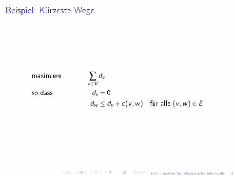
Beispiel: Kürzeste Wege
maximiere ∑v∈V
dv
so dass ds = 0
dw ≤ dv + c(v ,w) für alle (v ,w) ∈ E

KIT � Institut für Theoretische Informatik 9
Eine Anwendung � Tierfutter
I n Futtersorten,Sorte i kostet ci Euro/kg.
I m Anforderungen an gesundeErnährung (Kalorien, Proteine,Vitamin C,. . . ).Sorte i enthält aji Prozent destäglichen Bedarfs pro kg bzgl.Anforderung j
I Sei aji die i-te Komponente von
Vektor aj .
I De�niere xi alszu bescha�ende Menge von Sorte i
I LP-Lösung gibt eine kostenoptimale
�gesunde� Mischung.
KIT � Institut für Theoretische Informatik 10
Verfeinerungen
I Obere Schranken (Radioaktivität, Cadmium, Kuhhirn, . . . )
I Beschränkte Reserven (z. B. eigenes Heu)
I bestimmte abschnittweise lineare Kostenfunktionen (z. B. mitAbstand wachsende Transportkosten)
I Minimale Abnahmemengen
I die meisten nichtlinearen Kostenfunktionen
I Ganzzahlige Mengen (für wenige Tiere)
I Garbage in, Garbage out

KIT � Institut für Theoretische Informatik 11
Algorithmen und Implementierungen
I LPs lassen sich in polynomieller Zeit lösen [Khachiyan 1979]
I Worst case O(max(m,n)
7
2
)I In der Praxis geht das viel schneller
I Robuste, e�ziente Implementierungen sind sehr aufwändig
Fertige freie und kommerzielle Pakete
KIT � Institut für Theoretische Informatik 12
Ganzzahlige Lineare Programmierung
ILP: Integer Linear Program, lineares Programm mit derzusätzlichen Bedingung xi ∈ N.oft: 0/1 ILP mit xi ∈ {0,1}
MILP: Mixed Integer Linear Program, lineares Programm beidem einige Variablen ganzzahlig sein müssen.
Lineare Relaxation: Entferne die Ganzzahligkeitsbedingungen eines(M)ILP
KIT � Institut für Theoretische Informatik 13
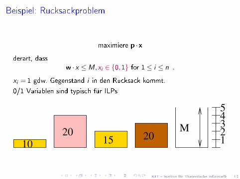
Beispiel: Rucksackproblem
maximiere p ·x
derart, dassw ·x ≤M,xi ∈ {0,1} for 1≤ i ≤ n .
xi = 1 gdw. Gegenstand i in den Rucksack kommt.
0/1 Variablen sind typisch für ILPs
10
2015
20M
2
45
3
1
KIT � Institut für Theoretische Informatik 14
Umgang mit (M)ILPs
− NP-schwer
+ Ausdrucksstarke Modellierungssprache
+ Es gibt generische Lösungsansätze, die manchmal gutfunktionieren
+ Viele Möglichkeiten für Näherungslösungen
+ Die Lösung der linearen Relaxation hilft oft, z. B. einfach runden.
+ Ausgefeilte Softwarepakete
Beispiel: Beim Rucksackproblem gibt es nur eine fraktionale Variable inder linearen Relaxation � Abrunden ergibt zulässige Lösung. Annäherndoptimal, falls Gewichte und Pro�te � Kapazität
KIT � Institut für Theoretische Informatik 15
Nie zurückschauen � Greedy-Algorithmen(deutsch: gierige Algorithmen, Ausdruck wenig gebräuchlich)
Idee: tre�e jeweils eine lokal optimale Entscheidung

KIT � Institut für Theoretische Informatik 16
Optimale Greedy-Algorithmen
I Dijkstras Algorithmus für kürzeste Wege
I Minimale SpannbäumeI Jarník-PrimI Kruskal
I Selection-Sort (wenn man so will)
Viel häu�ger, z.T. mit Qualitätsgarantien.Mehr: Vorlesungen Algorithmen II undApproximations- und Onlinealgorithmen

KIT � Institut für Theoretische Informatik 17
Beispiel: Rucksackproblem
Procedure roundDownKnapsacksort items by pro�t density pi
wi
�nd min{j : ∑
ji=1
wj >M}
// critical item
output items 1..j−1
Procedure greedyKnapsacksort items by pro�t density pi
wi
for i := 1 to n doif there is room for item i then
insert it into the knapsack
KIT � Institut für Theoretische Informatik 18
Dynamische Programmierung � Aufbau aus Bausteinen
Anwendbar, wenn das Optimalitätsprinzip gilt:
I Optimale Lösungen bestehen aus optimalen Lösungen fürTeilprobleme.
I Mehrere optimale Lösungen ⇒ es ist egal, welche benutzt wird.

KIT � Institut für Theoretische Informatik 19
Beispiel: Rucksackproblem
Annahme: ganzzahlige GewichteP(i ,C ):= optimaler Pro�t für Gegenstände 1,. . . ,iunter Benutzung von Kapazität ≤ C .
P(0,C ):= 0
Lemma:
∀1≤ i ≤ n : P(i ,C ) =max(P(i −1,C ),
P(i −1,C −wi )+pi )

KIT � Institut für Theoretische Informatik 20
Dynamische Programmierungauszufüllende Tabelle
Wdh. Lemma:
∀1≤ i ≤ n : P(i ,C ) =max(P(i −1,C ),
P(i −1,C −wi )+pi )
KIT � Institut für Theoretische Informatik 21
Beweis des Lemmas
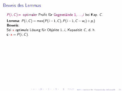
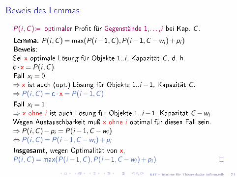
P(i ,C ):= optimaler Pro�t für Gegenstände 1,. . . ,i bei Kap. C .
Lemma: P(i ,C ) =max(P(i −1,C ),P(i −1,C −wi )+pi )Beweis:Sei x optimale Lösung für Objekte 1..i , Kapazität C , d. h.c ·x= P(i ,C ).
Fall xi = 0:⇒ x ist auch (opt.) Lösung für Objekte 1..i −1, Kapazität C .⇒ P(i ,C ) = c ·x= P(i −1,C )
Fall xi = 1:⇒ x ohne i ist auch Lösung für Objekte 1..i −1, Kapazität C −wi .Wegen Austauschbarkeit muÿ x ohne i optimal für diesen Fall sein.⇒ P(i ,C )−pi = P(i −1,C −wi )⇔ P(i ,C ) = P(i −1,C −wi )+pi
Insgesamt, wegen Optimalität von x,P(i ,C ) =max(P(i −1,C ),P(i −1,C −wi )+pi )

KIT � Institut für Theoretische Informatik 21
Beweis des Lemmas
P(i ,C ):= optimaler Pro�t für Gegenstände 1,. . . ,i bei Kap. C .
Lemma: P(i ,C ) =max(P(i −1,C ),P(i −1,C −wi )+pi )Beweis:Sei x optimale Lösung für Objekte 1..i , Kapazität C , d. h.c ·x= P(i ,C ).Fall xi = 0:⇒ x ist auch (opt.) Lösung für Objekte 1..i −1, Kapazität C .⇒ P(i ,C ) = c ·x= P(i −1,C )
Fall xi = 1:⇒ x ohne i ist auch Lösung für Objekte 1..i −1, Kapazität C −wi .Wegen Austauschbarkeit muÿ x ohne i optimal für diesen Fall sein.⇒ P(i ,C )−pi = P(i −1,C −wi )⇔ P(i ,C ) = P(i −1,C −wi )+pi
Insgesamt, wegen Optimalität von x,P(i ,C ) =max(P(i −1,C ),P(i −1,C −wi )+pi )

KIT � Institut für Theoretische Informatik 22
Berechung von P(i ,C ) elementweise:
P(i ,C ) =max(P(i −1,C ),P(i −1,C −wi )+pi )
Procedure knapsack(p, c, n, M)array P[0 . . .M] = [0, . . . ,0]bitarray decision[1 . . .n,0 . . .M] = [(0, . . . ,0), . . . ,(0, . . . ,0)]for i := 1 to n do
// invariant: ∀C ∈ {1, . . . ,M} : P[C ] = P(i −1,C )for C := M downto wi do
if P[C −wi ]+pi > P[C ] thenP[C ] := P[C −wi ]+pidecision[i ,C ] := 1

KIT � Institut für Theoretische Informatik 23
Rekonstruktion der Lösung
C := Marray x[1 . . .n]for i := n downto 1 do
x[i ] := decision[i ,C ]if x[i ] = 1 then C := C −wi
endforreturn x
Analyse:
Zeit: O(nM) pseudopolynomiell
Platz: M+O(n) Maschinenwörter plus nM bits.

KIT � Institut für Theoretische Informatik 24
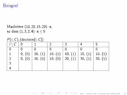
Beispiel
Maximiere (10,20,15,20) ·x,so dass (1,3,2,4) ·x≤ 5
P(i ,C ),(decision[i ,C ])i \C 0 1 2 3 4 5
0 0 0 0 0 0 01 0, (0) 10, (1) 10, (1) 10, (1) 10, (1) 10, (1)234
KIT � Institut für Theoretische Informatik 24
Beispiel
Maximiere (10,20,15,20) ·x,so dass (1,3,2,4) ·x≤ 5
P(i ,C ),(decision[i ,C ])i \C 0 1 2 3 4 5
0 0 0 0 0 0 01 0, (0) 10, (1) 10, (1) 10, (1) 10, (1) 10, (1)2 0, (0) 10, (0) 10, (0) 20, (1) 30, (1) 30, (1)34
KIT � Institut für Theoretische Informatik 24
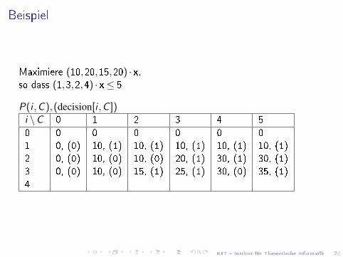
Beispiel
Maximiere (10,20,15,20) ·x,so dass (1,3,2,4) ·x≤ 5
P(i ,C ),(decision[i ,C ])i \C 0 1 2 3 4 5
0 0 0 0 0 0 01 0, (0) 10, (1) 10, (1) 10, (1) 10, (1) 10, (1)2 0, (0) 10, (0) 10, (0) 20, (1) 30, (1) 30, (1)3 0, (0) 10, (0) 15, (1) 25, (1) 30, (0) 35, (1)4

KIT � Institut für Theoretische Informatik 24
Beispiel
Maximiere (10,20,15,20) ·x,so dass (1,3,2,4) ·x≤ 5
P(i ,C ),(decision[i ,C ])i \C 0 1 2 3 4 5
0 0 0 0 0 0 01 0, (0) 10, (1) 10, (1) 10, (1) 10, (1) 10, (1)2 0, (0) 10, (0) 10, (0) 20, (1) 30, (1) 30, (1)3 0, (0) 10, (0) 15, (1) 25, (1) 30, (0) 35, (1)4 0, (0) 10, (0) 15, (0) 25, (0) 30, (0) 35, (0)


