53
Thin-sections of marine bivalve shells: a window to environmental reconstruction on a daily scale? Bachelorarbeit Gotje von Leesen Bremen, August 2014
Thin-sections of marine bivalve shells: a window to environmental
reconstruction on a daily scale?
Bachelorarbeit
Gotje von Leesen
Bremen, August 2014
I
Thin-sections of marine bivalve shells: a window to environmental reconstruction on a daily scale?
Bearbeitungszeitraum: 12. Mai bis 01. August 2014
vorgelegt dem Fachbereich 2 Biologie/ Chemie der Universität Bremen
Erstgutachter: Prof. Dr. Thomas Brey (Funktionelle Ökologie, AWI Bremerhaven)
Zweitgutachter: Prof. Dr. Claudio Richter (Bentho-Pelagische Prozesse, AWI Bremerhaven) verfasst von: Gotje von Leesen (Matrikelnummer: 2609231)

II
Eigenständigkeitserklärung
Hiermit bestätige ich, Gotje von Leesen, dass ich die vorliegende Arbeit selbstständig
verfasst und nur die angegebenen Quellen und Hilfsmittel verwendet wurden. Die Stellen
der Arbeit, die dem Wortlaut nach anderen Werken entnommen sind, wurden unter
Angabe der Quelle kenntlich gemacht.
Bremen, den 01.08.2014
III
Table of Contents
Danksagung VI
Zusammenfassung VII
Abstract VIII
1 Introduction 1 1.1 Aims and objectives 3
2 Material and Methods 5
2.1 Marine bivalve Arctica islandica 5 2.1.1 Taxonomy 5 2.1.2 Distribution 5 2.1.3 Physiology 5
2.1.4 Shell structure and biomineralization process 6 2.1.5 Annual and daily growth patterns 6
2.1.6 Shell material 7
2.2 Freshwater bivalve Unio sp. 8 2.2.1 Taxonomy 8
2.2.2 Distribution 8
2.2.3 Physiology 8
2.2.4 Shell material 9
2.3 Localities 9
2.4 Thin–sections of bivalve shells 12 2.4.1 Lapping of glass-slides 12
2.4.2 Sample preparation 13
2.4.3 Coating 13
2.4.4 Cutting 13
2.4.5 Embedding 14
2.4.6 Lapping and polishing of shell sections 15
2.4.7 Trial and error approaches 16
2.5 Additional attempts to improve the visualization of microincrements 18
2.5.1 Etching of thin-section with Mutvei’s solution 18
2.5.2 Bleaching of thin-section with hydrogen peroxide (H2O2) 18
2.6 Visualization techniques 18
2.6.1 Transmitted and reflected light microscopy 18
2.6.2 Scanning electron microscope (SEM) 19
IV
2.7 Thick-sections of marine bivalve shells 20
2.8 Removal of noise in growth records 20
3 Results 21
3.1 Thin-section preparation 21 3.1.1 Arctica islandica 21
3.1.2 Unio sp. 21
3.2 Additional attempts to improve the visualization of microincrements 21 3.2.1 Etching of thin-section with Mutvei’s solution 21
3.2.2 Bleaching of thin-section with hydrogen peroxide (H2O2) 22
3.3 Visualization techniques 22
3.3.1 Transmitted and reflected light microscopy 23
3.3.2 Scanning electron microscope (SEM) 23
3.4 Measurements of microincrements 23 3.4.1 Arctica islandica 23
3.4.2 Unio sp. 26
3.4.3 Comparison between Arctica islandica and Unio sp. 30
4 Discussion 31
4.1 Thin-section preparation 31 4.1.1 Arctica islandica 31
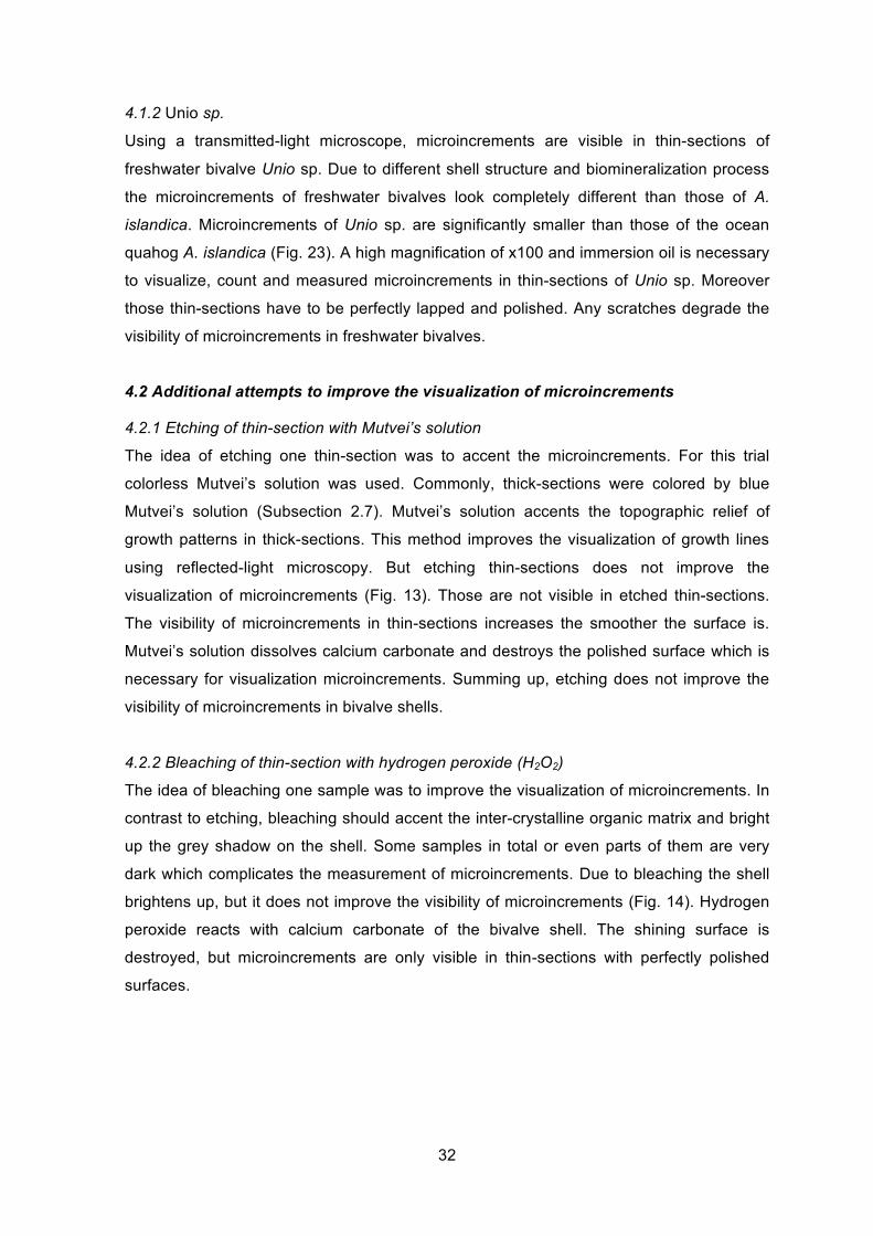
4.1.2 Unio sp. 32
4.2 Additional attempts to improve the visualization of microincrements 32
4.2.1 Etching of thin-section with Mutvei’s solution peroxide (H2O2) 32
4.2.2 Bleaching of thin-sections with hydrogen 32
4.3 Visualization techniques 33 4.3.1 Transmitted and reflected light microscopy 33
4.3.2 Scanning electron microscope (SEM) 33
4.4 Measurements of microincrements 33 4.4.1 Arctica islandica 33
4.4.2 Unio sp 34
4.4.3 Comparison between Arctica islandica and Unio sp. 35
5 Conclusions 36
6 Outlook 37

V
References 38
Appendix 43
VI
Danksagung
Bei folgenden Personen möchte ich mich für Ihre Unterstützung in der Zeit der
Bachelorarbeit bedanken. Sie haben mein fachliches Wissen erweitert, mich betreut und
mich die teilweise stressige Zeit der Bachelorarbeit überstehen lassen.
Mein Dank geht an…
… Prof. Dr. Thomas Brey, meinem Erstgutachter, für die großartige Möglichkeit am Alfred-
Wegener-Institut meine Bachelorarbeit zu schreiben und die Betreuung während dieser
Zeit.
… Prof. Dr. Claudio Richter, der sich sofort bereit erklärt hat, die Aufgabe des
Zweitgutachters zu übernehmen.
… Dr. Gernot Nehrke, für die fachliche Unterstützung und Bereitstellung zahlreicher
Maschinen zur Herstellung von Dünnschliffen.
… Lars Beierlein. Einfach vielen Dank für alles, insbesondere für die tolle Betreuung
während meiner Bachelorarbeit! Ich wünsche dir für deine weitere wissenschaftliche
Karriere alles Gute.
… Kerstin Beyer, für deine herzliche Art. Unermüdlich hast du überlegt, wie man die
Mikroinkremente besser sichtbar machen kann. Vielen Dank für deine Mühen!
… ein ganz besonderer Dank geht an meine Eltern. Ihr ermöglicht mir nicht nur meinen
Traum zu erfüllen, sondern wart und seid immer für mich da. Danke für all die Telefonate,
in denen ich euch von meiner Arbeit erzählt habe.
… all meinen lieben Freunden, ob in Bremen oder aus der alten Heimat, die mich auf
unterschiedliche Art und Weise auf meinem Weg bis hierher unterstützt und begleitet
haben. Ich sage einfach: danke! Ein besonderer Dank geht an Marius Lang – dafür, dass
du immer für mich da bist, wenn ich dich brauche. Für die Ablenkungen während der
Bachelorarbeit, die ab und an nötig waren und für die gesamte Zeit des Bachelor-
Studiums.
VII
Zusammenfassung
„Bioarchive“ sind Organismen, die während ihres Lebens Hartstrukturen bilden, die über
den Tod des Organismus hinaus erhalten bleiben und aus deren anatomischer,
morphologischer und chemischer Beschaffenheit Informationen über Umweltbedingungen
zu Lebzeiten des Organismus gewonnen werden können. Beispiele für Bioarchive sind
Krusten-Rotalgen (Skelette), Korallen (Skelette) und auch Muscheln, deren Schalen sich
durch ihre sehr hohe Auflösung für Studien in der Sclerochronologie eignen. Im
Allgemeinen beschäftigt sich diese Wissenschaft mit Wachstumsmustern und chemischen
Beschaffenheit in Hartstrukturen der Bioarchive. Verschiedene Proxies, wie z.B. die Breite
von Jahresinkrementen oder das Verhältnis von stabilen Sauerstoffisotopen (δ18O),
können entschlüsselt werden, um die in den Hartschalen enthaltende Information zu
„lesen“. Durch die weite geografische Verbreitung der Islandmuschel Arctica islandica und
ihrer Langlebigkeit eignet sich diese besonders für solche Studien. Zuwachsraten, die
anhand der Inkremente ausgemessen werden und die geochemische Eigenschaften des
Schalenkarbonats geben Auskunft über Umweltfaktoren wie Wassertemperatur, Nahrung,
Salinität und Wasserverschmutzung.
Einige Studien haben gezeigt, dass die tägliche Wachstumsrate in verschiedenen
Mollusken im Verlaufe eines Jahres variiert. Schöne et al. (2005a) berichten, dass
Mikroinkremente täglichen Zuwachs anzeigen. Mit Hilfe einer geeigneten Methode ist es
mögliche die Breite dieser Mikroinkremente zu messen und daraus Rückschlüsse über
Wachstumstrends und Klimarekonstruktion auf täglicher Basis zu erhalten.
Um diese Mikroinkremente zu visualisieren habe ich Dünnschliffe der marinen Muschelart
A. islandica und der Süßwassermuschel Unio sp. angefertigt. Da zur
Dünnschliffherstellung von Muschelschalen kein Standardprozedere existiert, war das Ziel
dieser Arbeit, eine geeignete Methode zur Herstellung dieser zu etablieren. Hierzu wurden
unter anderem verschiedene Ansätze zur Einbettung, Anätzen, Bleichen und Visualisieren
von Mikroinkrementen getestet.
Tägliche Mikroinkremente sind mittels der Dünnschliffe in A. islandica, als auch in Unio
sp. sichtbar. Die Mikroinkrementenbreiten in den Süßwassermuscheln sind hierbei
wesentlich kleiner (durchschnittlich 1,5 µm) als die der Islandmuschel (durchschnittlich
12,5 µm), dennoch sind sie in Unio sp. deutlich sichtbarer und können durchgehend
gemessen werden. Die Visualisierung der Mikroinkremente in A. islandica ist wesentlich
schwieriger und bedarf weiterer Ansätze im Labor (siehe Outlook Kapitel).
Mikroinkrementmessungen in der Süßwassermuschel Unio sp. zeigen dagegen ein
großes Potential und können mit den hier beschriebenen Methoden zukünftig als
potentieller Umweltproxy etabliert werden.
VIII
Abstract
“Bioarchives” are organisms, which form hard parts over the course of their lifetime that
remain even after the death of the organism. Environmental conditions prevailed during
the lifetime of the bioarchives can be approximated from anatomical, morphological and
geochemical properties on the shell. For instance, shell growth rates constitute a “proxy”
of general living conditions, oxygen isotope ratios (δ18O) are an established proxy of water
temperature, and shell content of heavy metals or of organic constituents can be
indicative specific pollution histories. Due to their high resolution, bivalve shells are well
suited for sclerochronological studies. Generally, this science focuses on growth rates and
chemical properties of hard parts. The ocean quahog Arctica islandica is suited as a
bioarchive due to its broad geographic distribution and longevity.
This study looks at growth patterns in the shells of the bivalve A. islandica (marine) and
Unio sp. (freshwater). The objective was to establish standard procedures for shell
preparation to visualize shell increments formed on a daily basis (“microincrements”).
In order to visualize microincrements thin-sections of the marine bivalve A. islandica and
the freshwater bivalve Unio sp. were prepared. Therefore, different attempts for
embedding, etching, bleaching and visualization were tested.
Microincrements are visible in thin-sections of both genera. The microincrements of the
freshwater mussel Unio sp. are significantly smaller (1.5 µm on average) than those of A.
islandica (12.5 µm on average). However, microincrements in Unio sp. are more easily
recognizable and can be measured consecutively over a range of more than one year.
The visualization of microincrements in A. islandica remained more challenging and
therefore additional attempts such as bleaching, etching and additional visualization
techniques were tested for their potential to improve the visualization of microincrements.
The visualization of microincrements in A. islandica still needs further improvement before
measured microincrement widths can be correlated to environmental data. However, Unio
sp. seems to have great potential and can be used as a window to reconstruct
environmental data on a daily scale in the future.
1
1 Introduction
The knowledge how ecosystems react to changing environmental conditions is essential
for well-constrained predictive climate-models (Schöne, 2013).
Bioarchives like red-coralline algae (skeleton), corals (skeleton) and mollusks are living
organisms which from hard parts during their lifetime (Marchitto et al., 2000). Anatomical,
morphological and geochemical properties give information about environmental
conditions prevailing during the lifetime of those bioarchives. They help to understand
climate changes on time scales up to centuries with an annual to sub-annual resolution
(Markwick, 2007). In the case of mollusks the hard parts are usually precipitated in the
form of calcium carbonate. Shell growth rates constitute a “proxy” of general living
conditions like salinity (Davis and Calabrese, 1964), water temperature (Kennish and
Olsson, 1975) and food (Page and Hubbard, 1987). Oxygen isotope ratios (δ18O) are an
established proxy of water temperature (Schöne et al., 2005b), and shell content of heavy
metals or of organic constituents can be indicative specific pollution histories (Krause-
Nehring et al., 2012). Proxies were used to encode the recorded climate data.
According to Boecker (2000) climate change is often modulated by seasonality changes in
periodicities in the Earth’s orbital elements. Other archives like sediment and ice cores
also exist. Sediment cores are the climate archives that cover the longest time spans (up
to millions of years), but they have limited temporal resolution of about a decade usually
and down to a few years at best (e.g. Jiang et al., 2005; Eiríksson et al., 2006). Ice cores
may span several hundreds of thousands of years, but have an annual solution at best.
Hence both archive types hardly provide information on annual scales and not at all at
sub-annual / seasonal variability. Consequently, they cannot give information about sub-
annual and seasonal dynamics, but this is important for our understanding of past climate
dynamics and for proper modeling of paleo and future climate states. This explains our
need for archives with annual and better temporal resolution.
Analogous to sclerochronology, dentrochronologists use trees as archives. Schweingruber
et al. (1991) have shown that tree rings are suitable proxies for summer air temperature
and precipitation on land. Those proxies do not have a sufficient resolution to determine
seasonal variability in environmental parameter (Schöne et al., 2005a). Further, data
obtained from tree rings are summer-biased and do not provide information about marine
settings. Due to short life spans microfossils (e.g. foraminifera), obtained from low
resolution marine sediment cores do not provide information on annual or sub-annual
scales (Schöne, 2005b).
2
The ocean quahog Arctica islandica is suited for sclerochronological studies due to its
broad geographic distribution (Schöne et al., 2005b) and its longevity (Schöne, 2013).
Several studies about shell growth on annual (e.g. Schöne et al. 2005; Schöne, 2013) and
seasonal resolution describe the multitude of research possibilities on paleoclimate, water
quality monitoring and ecology (c.f. Schöne, 2013). Seasonal resolution is a unique
feature in bivalve shells. Here, by identifying and looking at so called microincrements,
even a daily resolution can be achieved.
Schöne et al. (2005a) present a study about daily growth rates in A. islandica. However,
little is known about shell growth on a daily scale due to missing appropriate visualizing
techniques. Due to higher growth rates in the early stages of life of mollusks,
microincrements are expected to be best visible in the earliest ontogenetic years
(Cargnelli et al., 1999). Going from the umbonal area to the ventral margin and in the
direction of growth the number of visible microincrements decreases. Daily growth
increments are orientated parallel to the more prominent annual growth lines. Clark et al.
(1975) demonstrate that shell growth and biomineralization processes are controlled by
biological clocks. Dependent on the species they can take place on various time-scales.
For two species of pectinids it is shown that they form growth lines on a daily periodicity.
The potential of master chronologies providing environmental information over hundreds
or even thousands of years is described by Jones et al. (1989). For example, a 489-year
marine master chronology was used to reconstruct the marine climate in the Irish Sea
(Butler et al., 2010). Furthermore, statoliths in squids record their environment with daily
precision (Arkhipkin, 2005). Goodwin et al. (2001) used stable oxygen isotope
measurements in combination with microincrement widths to obtain paleoclimatic
information on sub-weekly and sub-monthly scales. These examples show the importance
of studies of bio archives on sub-annual levels.

3
1.1 Aims and Objectives
This study focuses on the questions if thin-sections are a suitable method for visualizing
microincrements in marine and freshwater bivalve shells, how a standard procedure to
prepare such thin-section can be established and if obtained microincrement
measurements can be used as a window to reconstruct environmental parameters on a
daily scale. In detail, the following issues and questions should be addressed and
answered in this study:
Is it possible to prepare thin-sections of marine shells of Arctica islandica?
Is it possible to prepare thin-sections of freshwater bivalve of Unio sp.?
How to establish a standard procedure to prepare thin-sections of bivalve shells?
Are there any differences in the preparation of thin-sections between both
species?
Are thin-sections a suitable method for visualizing microincrements?
Which microscope methods are the best suited for visualizing microincrements?
Can bleaching and etching procedures help to visualize microincrements?
Which growth trends can be seen within one year?
Can microincrements be measured and correlated to environmental datasets?
What is the difference of microincrement widths between species?
4
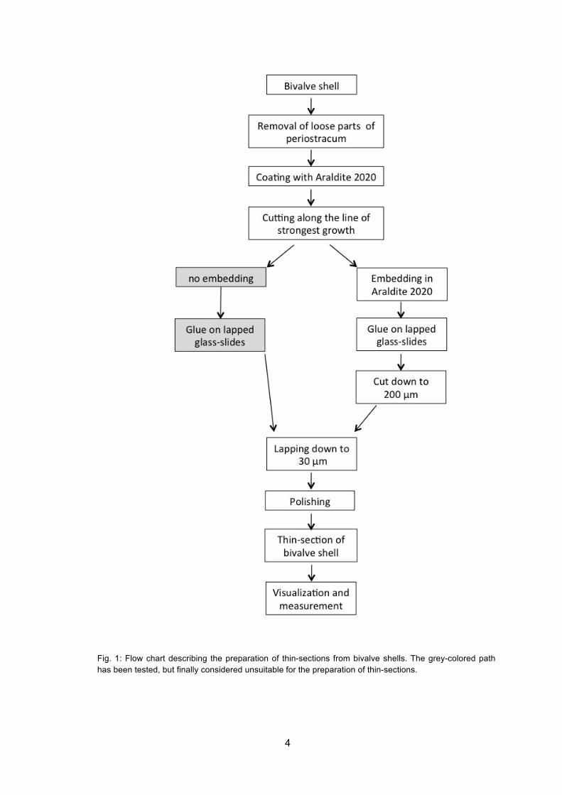
Fig. 1: Flow chart describing the preparation of thin-sections from bivalve shells. The grey-colored path has been tested, but finally considered unsuitable for the preparation of thin-sections.
5
2 Material and Methods
2.1 Marine bivalve Arctica islandica
The ocean quahog Arctica islandica is the “longest lived, non-colonial animal of the world”
(Wanamaker et al., 2008).
2.1.1 Taxonomy
Table 1 shows the verified taxonomic range of Arctica islandica, which has previously
been known as Cyprina islandica.
Table 1: Taxonomic range of Arctica islandica (http://www.itis.gov/, checked: 24.06.2014).
Kingdom Animalia
Subkingdom Bilateria
Phylum Mollusca
Class Bivalvia (Linnaeus, 1758)
Subclass Heterodonta (Neumayr, 1884)
Order Veneroida (H. Adams and A. Adams, 1856)
Superfamily Arcticoidea (Newton, 1891)
Family Arcticidae (Newton, 1891)
Genus Arctica (Schumacher, 1817)
Species Arctica islandica (Linnaeus, 1767)
2.1.2 Distribution
This species can be found in the temperate/boreal North Atlantic (Thórarinsdóttir and
Einarsson, 1996), ranging from the Bay of Cadiz in Spain, north to Iceland in the northeast
Atlantic, and from Cape Hatteras in North Carolina, USA, to the Canadian Arctic in the
northwest Atlantic (Nicol, 1951; Merrill and Ropes, 1969; Abbott, 1974; Brey et al., 1990;
Witbaard et al., 1999). Thereby, the water depth range of A. islandica varies between 10 –
280 m (Thompson et al., 1980a). Occasionally, the ocean quahog can be found in depths
of 500 m (Nicol, 1951).
2.1.3 Physiology
The modern distribution for A. islandica implies a water temperature range from 1°-16°C
(Golikov and Scarleto, 1973). Winter (1969) have demonstrated that the filtration rates are
reduced by 50% when the temperature decreases from 12° to 4°C and respectively
double when temperature increases from 4° to 14°C. A. islandica do not survive for more
than a few hours at water temperatures below 0°C and consequently it is assumed a
6
boreal genus and not an arctic one (Nicol, 1951). Further, this species tolerates salinity
ranges from 22 to 35 PSU (Winter, 1969).
Generally categorized as a suspension feeder (Cargnelli et al., 1999), Morton (2011)
reclassifies the ocean quahog as a specialized deposit feeder (c.f. Schöne, 2013).
Although the typical long siphons are missing, the sinking carbon from the suspended
particles of epibenthic organic material, which characterizes the seabed and the rich
surface water, is collected.
According to Lutz et al. (1981) A. islandica most commonly inhabits muddy and sandy
sediments (Nicol, 1951), but also settles down to a wide array of other substrate types
where it lives borrowed in the top 5 cm of the substrate (Morton, 2011). The main
predators for young individuals of A. islandica are cod and lab. The mortality rate in
medium sized specimens decreases and due to senility increases again for old animals
(Brey et al., 1990).
2.1.4 Shell structure and biomineralization process
The surface of the outer shell layer of the ocean quahog A. islandica is covered by the
periostracum, which protects the marine bivalve against dissolution as well as microbial
attack (Wilbur and Saleuddin, 1983). The shell of A. islandica consists of calcium
carbonate, which is largely aragonitic and structured in three layers: the outer and the
inner shell layer as well as the myostracum. For sclerochronological studies the outer
shell layer or the umbonal hinge plate are used. The shell is secreted by the mantle. In
general, “the mantle and its outer epithelium, the periostracum and the interface between
the outer epithelium, the periostracum and the growing shell” are necessary for the
calcification process of the shell (Marin et al., 2012).
2.1.5 Annual and daily growth patterns
Annual and daily-scale growth patterns become visible in marine bivalve shells such as A.
islandica due to interrupted growth. Moreover they do not grow at the same rate during
their lifespan which explains more narrow annual increment widths in ontogenetic older
shell portions. Growth rates decrease throughout the lifetime caused by biological aging.
In general, variability in growth is a result from changes in physiology and environment
(Schöne, 2013).
The distance of the alternating pattern of one thick growth line (GB1 = growth break) and
one thinner one, GB2, is defined as an annual increment (Schöne et al., 2005a).
7
GB1 is formed in fall or early winter and is linked to the spawning cycle. Specimens
belonging to one population are synchronous in forming GB1. During the period of
formation of GB1 the rate of shell growth is relatively slow, whereas the growth rate is
most rapidly in late spring and early summer. This concludes that the growth rates of A.
islandica are not consistent throughout the year. This was also described by Schöne et al.
(2005b). They could show that shell growth starts before winter minimum temperatures
are reached and stops after the summer maximum. Moreover, shell growth is uniformly
slow during the times with hottest and coldest seasonal temperatures (Jones, 1980, 1981;
Thompson et al., 1980). Schöne et al. (2005a) suppose that the period of growth takes
eight months in shells from the North Sea. Growing season ends in autumn / winter. As a
conclusion, temperature seems to trigger shell growth either directly or indirectly.
Thompson et al. (1980a) hypothesize that immature animals of A. islandica mimic the
annual reproduction cycle. This would explain the interruption or at least the slow-down of
shell growth and therefore the formation of growth rings.
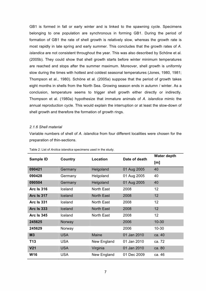
2.1.6 Shell material
Variable numbers of shell of A. islandica from four different localities were chosen for the
preparation of thin-sections.
Table 2: List of Arctica islandica specimens used in the study.
Sample ID Country Location Date of death Water depth
[m]
090421 Germany Helgoland 01 Aug 2005 40
090428 Germany Helgoland 01 Aug 2005 40
090504 Germany Helgoland 01 Aug 2005 40
Arc Is 316 Iceland North East 2008 12
Arc Is 317 Iceland North East 2008 12
Arc Is 331 Iceland North East 2008 12
Arc Is 333 Iceland North East 2008 12
Arc Is 345 Iceland North East 2008 12
245625 Norway 2006 10-30
245629 Norway 2006 10-30
M3 USA Maine 01 Jan 2010 ca. 40
T13 USA New England 01 Jan 2010 ca. 72
V21 USA Virginia 01 Jan 2010 ca. 80
W16 USA New England 01 Dec 2009 ca. 46
8
2.2 Freshwater bivalve Unio sp.
Additionally, thin-sections of two freshwater shells of the genus Unio were prepared. Both
have been collected from the Lago Maggiore, Italy.
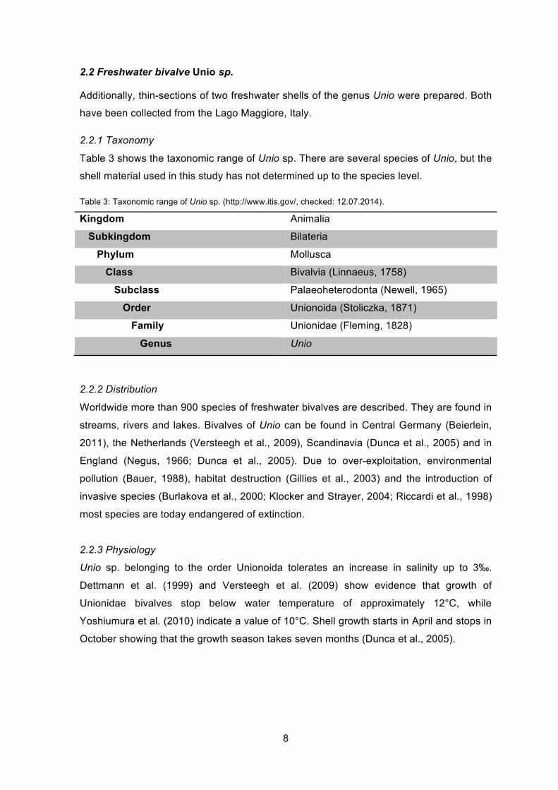
2.2.1 Taxonomy
Table 3 shows the taxonomic range of Unio sp. There are several species of Unio, but the
shell material used in this study has not determined up to the species level.
Table 3: Taxonomic range of Unio sp. (http://www.itis.gov/, checked: 12.07.2014).
Kingdom Animalia
Subkingdom Bilateria
Phylum Mollusca
Class Bivalvia (Linnaeus, 1758)
Subclass Palaeoheterodonta (Newell, 1965)
Order Unionoida (Stoliczka, 1871)
Family Unionidae (Fleming, 1828)
Genus Unio
2.2.2 Distribution
Worldwide more than 900 species of freshwater bivalves are described. They are found in
streams, rivers and lakes. Bivalves of Unio can be found in Central Germany (Beierlein,
2011), the Netherlands (Versteegh et al., 2009), Scandinavia (Dunca et al., 2005) and in
England (Negus, 1966; Dunca et al., 2005). Due to over-exploitation, environmental
pollution (Bauer, 1988), habitat destruction (Gillies et al., 2003) and the introduction of
invasive species (Burlakova et al., 2000; Klocker and Strayer, 2004; Riccardi et al., 1998)
most species are today endangered of extinction.
2.2.3 Physiology
Unio sp. belonging to the order Unionoida tolerates an increase in salinity up to 3‰.
Dettmann et al. (1999) and Versteegh et al. (2009) show evidence that growth of
Unionidae bivalves stop below water temperature of approximately 12°C, while
Yoshiumura et al. (2010) indicate a value of 10°C. Shell growth starts in April and stops in
October showing that the growth season takes seven months (Dunca et al., 2005).
9
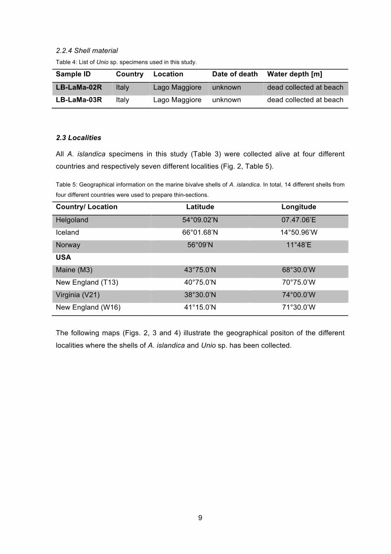
2.2.4 Shell material Table 4: List of Unio sp. specimens used in this study.
Sample ID Country Location Date of death Water depth [m]
LB-LaMa-02R Italy Lago Maggiore unknown dead collected at beach
LB-LaMa-03R Italy Lago Maggiore unknown dead collected at beach
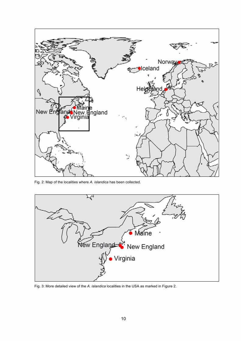
2.3 Localities
All A. islandica specimens in this study (Table 3) were collected alive at four different
countries and respectively seven different localities (Fig. 2, Table 5).
Table 5: Geographical information on the marine bivalve shells of A. islandica. In total, 14 different shells from
four different countries were used to prepare thin-sections.
Country/ Location Latitude Longitude
Helgoland 54°09.02’N 07.47.06’E
Iceland 66°01.68’N 14°50.96’W
Norway 56°09’N 11°48’E
USA
Maine (M3) 43°75.0’N 68°30.0’W
New England (T13) 40°75.0’N 70°75.0’W
Virginia (V21) 38°30.0’N 74°00.0’W
New England (W16) 41°15.0’N 71°30.0’W
The following maps (Figs. 2, 3 and 4) illustrate the geographical positon of the different
localities where the shells of A. islandica and Unio sp. has been collected.
10
Fig. 2: Map of the localities where A. islandica has been collected.
Fig. 3: More detailed view of the A. islandica localities in the USA as marked in Figure 2.
11
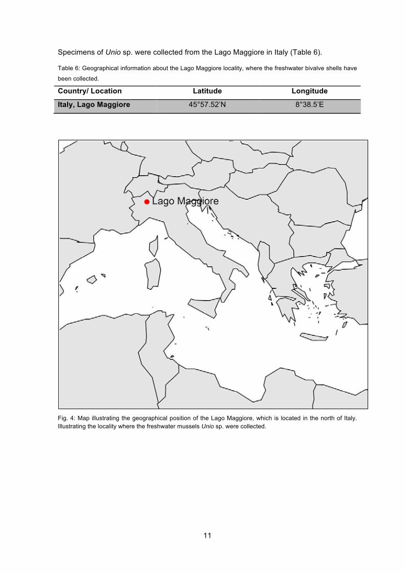
Specimens of Unio sp. were collected from the Lago Maggiore in Italy (Table 6).
Table 6: Geographical information about the Lago Maggiore locality, where the freshwater bivalve shells have
been collected.
Country/ Location Latitude Longitude
Italy, Lago Maggiore 45°57.52’N 8°38.5’E
Fig. 4: Map illustrating the geographical position of the Lago Maggiore, which is located in the north of Italy. Illustrating the locality where the freshwater mussels Unio sp. were collected.
12
2. 4 Thin-sections of bivalve shells
I prepared thin-sections to visualize daily increments in bivalve shells. Several steps are
required to visualize them. The idea of preparing a thin-section is that shell material is
glued on a glass-slide and then lapped down to ~30 µm. However, on the micrometer
scale glass-slides are not plane-parallel. Therefore, the glass-slides have to be lapped
first. This is conducted to assure that they are equally thick throughout.
2.4.1 Lapping of glass-slides
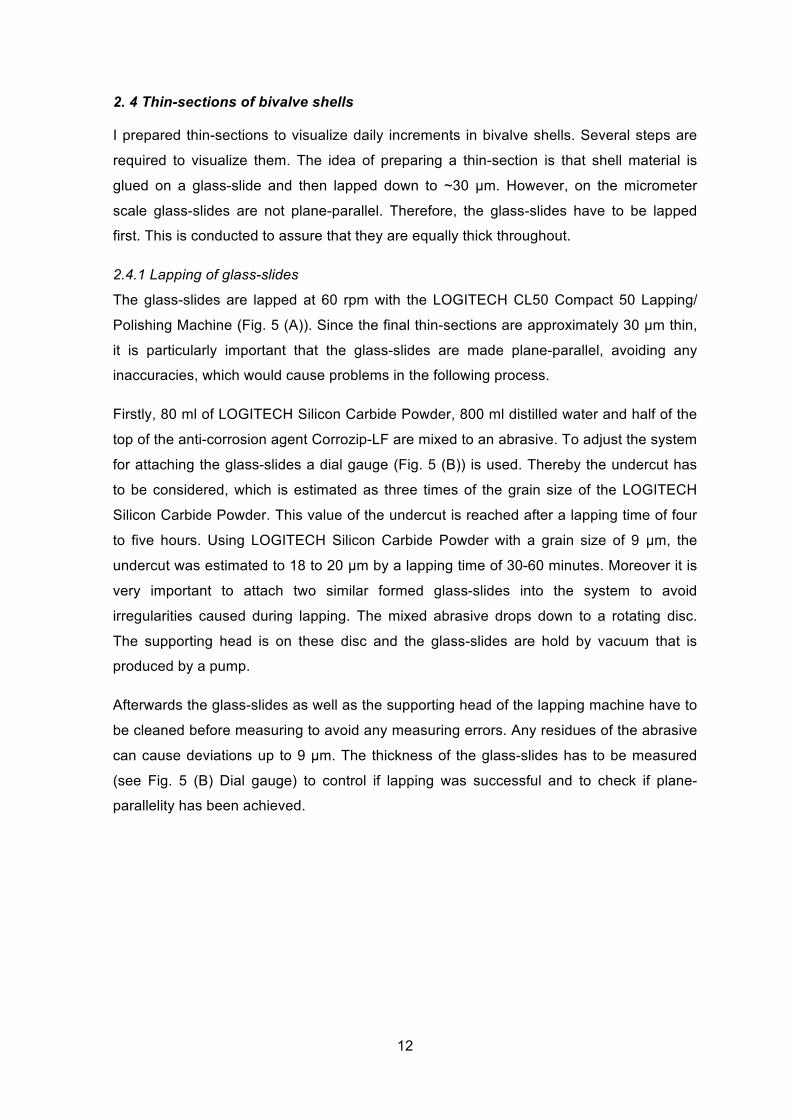
The glass-slides are lapped at 60 rpm with the LOGITECH CL50 Compact 50 Lapping/
Polishing Machine (Fig. 5 (A)). Since the final thin-sections are approximately 30 µm thin,
it is particularly important that the glass-slides are made plane-parallel, avoiding any
inaccuracies, which would cause problems in the following process.
Firstly, 80 ml of LOGITECH Silicon Carbide Powder, 800 ml distilled water and half of the
top of the anti-corrosion agent Corrozip-LF are mixed to an abrasive. To adjust the system
for attaching the glass-slides a dial gauge (Fig. 5 (B)) is used. Thereby the undercut has
to be considered, which is estimated as three times of the grain size of the LOGITECH
Silicon Carbide Powder. This value of the undercut is reached after a lapping time of four
to five hours. Using LOGITECH Silicon Carbide Powder with a grain size of 9 µm, the
undercut was estimated to 18 to 20 µm by a lapping time of 30-60 minutes. Moreover it is
very important to attach two similar formed glass-slides into the system to avoid
irregularities caused during lapping. The mixed abrasive drops down to a rotating disc.
The supporting head is on these disc and the glass-slides are hold by vacuum that is
produced by a pump.
Afterwards the glass-slides as well as the supporting head of the lapping machine have to
be cleaned before measuring to avoid any measuring errors. Any residues of the abrasive
can cause deviations up to 9 µm. The thickness of the glass-slides has to be measured
(see Fig. 5 (B) Dial gauge) to control if lapping was successful and to check if plane-
parallelity has been achieved.
13
Fig. 5: (A) Lapping/ Polishing Machine and (B) Dial gauge.
2.4.2 Sample preparation
First of all, the shells are cleaned by removing sediment and loose parts of periostracum
with a toothbrush to prevent that superglue drops off afterwards.
2.4.3 Coating
Afterwards, the shell has to be coated twice with Araldite 2020 to prevent the shell from
breaking during cutting. Araldite has to set hard for 24 hours before it can be coated
again.
2.4.4 Cutting
A first cut has to be done 1 cm left or right of the line of strongest growth to get a straight
line which is necessary for fixing the shell material to a metal block. Therefore, the cut
surface has to be grind with sandpaper with grain size of 20 µm to obtain a flat surface
parallel to LSG (= line of longest growth). Following individual valves are fixed by
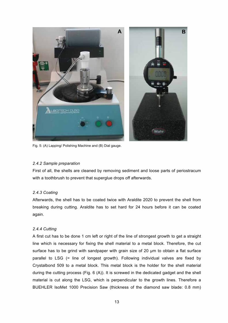
Crystalbond 509 to a metal block. This metal block is the holder for the shell material
during the cutting process (Fig. 6 (A)). It is screwed in the dedicated gadget and the shell
material is cut along the LSG, which is perpendicular to the growth lines. Therefore a
BUEHLER IsoMet 1000 Precision Saw (thickness of the diamond saw blade: 0.8 mm)
A B
14
(Fig. 6 (B)) is used. This side of LSG is grinded with waterproof sandpaper grade 1200
(grain size 15 µm) and following embedded in Araldite.
Fig. 6: Low-speed saw used for cutting bivalve shells on the line of strongest growth. (A) One shell of A. islandica is glued on a metal block with Crystalbond. (B) Shells were cut with a rotation speed of 225 rpm.
2.4.5 Embedding
Rings of aluminum covered by Teflon are fixed by screws to a plate. Additionally, samples
were fixated by superglue to avoid that they tip over. After this pretreatment, Araldite 2020
has been filled into the aluminium rings until bivalve shells have been covered. Like this
they have been set to harden in an oven at about 50°C for about 24 hours.
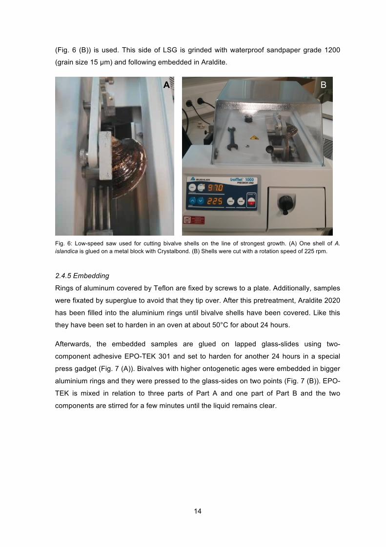
Afterwards, the embedded samples are glued on lapped glass-slides using two-
component adhesive EPO-TEK 301 and set to harden for another 24 hours in a special
press gadget (Fig. 7 (A)). Bivalves with higher ontogenetic ages were embedded in bigger
aluminium rings and they were pressed to the glass-sides on two points (Fig. 7 (B)). EPO-
TEK is mixed in relation to three parts of Part A and one part of Part B and the two
components are stirred for a few minutes until the liquid remains clear.
A B
15
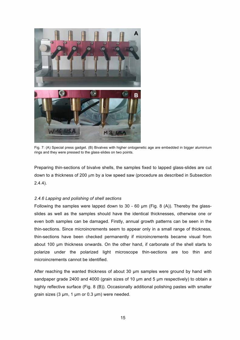
Fig. 7: (A) Special press gadget. (B) Bivalves with higher ontogenetic age are embedded in bigger aluminium rings and they were pressed to the glass-slides on two points.
Preparing thin-sections of bivalve shells, the samples fixed to lapped glass-slides are cut
down to a thickness of 200 µμm by a low speed saw (procedure as described in Subsection
2.4.4).
2.4.6 Lapping and polishing of shell sections
Following the samples were lapped down to 30 - 60 µm (Fig. 8 (A)). Thereby the glass-
slides as well as the samples should have the identical thicknesses, otherwise one or
even both samples can be damaged. Firstly, annual growth patterns can be seen in the
thin-sections. Since microincrements seem to appear only in a small range of thickness,
thin-sections have been checked permanently if microincrements became visual from
about 100 µm thickness onwards. On the other hand, if carbonate of the shell starts to
polarize under the polarized light microscope thin-sections are too thin and
microincrements cannot be identified.
After reaching the wanted thickness of about 30 µm samples were ground by hand with
sandpaper grade 2400 and 4000 (grain sizes of 10 µm and 5 µm respectively) to obtain a
highly reflective surface (Fig. 8 (B)). Occasionally additional polishing pastes with smaller
grain sizes (3 µm, 1 µm or 0.3 µm) were needed.
A
B
B

16
Fig. 8: (A) Bottom side of the supporting head of the lapping and polishing machine. The two thin-sections are cut down to 200 µm and currently in the lapping process. (B) Sandpaper with different grain size is used to grind and polish the thin-sections. For this, glass-slides were mounted into the red holder and moved in irregularly circles over the sandpaper.
2.4.7 Trial and error approaches
No embedding
An approximately 1 mm thick part of the valve is glued on a lapped glass-slide with EPO-
TEK 301 with the LSG directly glued on the glass-slide (Fig. 9 (A)). This is done to ensure
that the growth pattern later on identified is directly on the LSG rather than 1 mm away.
Samples have been lapped until being approximately 35 µm thin. Several problems
occurred and have led to the conclusion that this method is not suitable for the preparation
of thin-sections. Scratches caused by the saw have to be removed by grinding the shell
material before gluing it onto the glass-slides, but this turned out to not be feasible without
damaging the bivalve section. Moreover it was not possible to glue the thin-sections of the
bivalve shell plan-parallel to the lapped glass-slides. Due to uneven pressure onto the
sample and especially towards the ends of the shell (Fig. 9 (B)) by the pressure gadget
device (Fig. 7) the preparation of plane-parallel thin-section failed.
A B
17
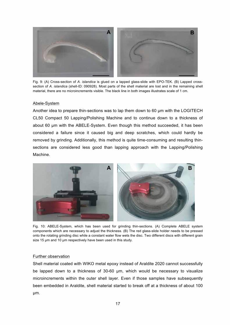
Fig. 9: (A) Cross-section of A. islandica is glued on a lapped glass-slide with EPO-TEK. (B) Lapped cross-section of A. islandica (shell-ID: 090928). Most parts of the shell material are lost and in the remaining shell material, there are no microincrements visible. The black line in both images illustrates scale of 1 cm.
Abele-System
Another idea to prepare thin-sections was to lap them down to 60 µm with the LOGITECH
CL50 Compact 50 Lapping/Polishing Machine and to continue down to a thickness of
about 60 µm with the ABELE-System. Even though this method succeeded, it has been
considered a failure since it caused big and deep scratches, which could hardly be
removed by grinding. Additionally, this method is quite time-consuming and resulting thin-
sections are considered less good than lapping approach with the Lapping/Polishing
Machine.
Fig. 10: ABELE-System, which has been used for grinding thin-sections. (A) Complete ABELE system components which are necessary to adjust the thickness. (B) The red glass-slide holder needs to be pressed onto the rotating grinding disc while a constant water flow wets the disc. Two different discs with different grain size 15 µm and 10 µm respectively have been used in this study.
Further observation
Shell material coated with WIKO metal epoxy instead of Araldite 2020 cannot successfully
be lapped down to a thickness of 30-60 µm, which would be necessary to visualize
microincrements within the outer shell layer. Even if those samples have subsequently
been embedded in Araldite, shell material started to break off at a thickness of about 100
µm.
A B
A B
18
2.5 Additional attempts to improve the visualization of microincrements
Several additional laboratory steps have been tested to increase the visibility in thin-
sections. As such it was tested if the microincrements become better visible after cleaning
and rinsing in an ultrasonic bath. Two samples were rinsed for 10 min with settings
chosen as follows: function: sweep, frequency: 35 kHz, power: 100% and heating off. No
difference or improvement could be seen afterwards. Furthermore, different chemicals as
well as further visualization techniques were tested and are described in the following.
2.5.1 Etching of thin-section with Mutvei’s solution
One thin-section of A. islandica (sample-ID: AI-WaHe-25R) was etched in colorless
Mutvei’s solution (Schöne, 2005a) for 10 minutes at room temperature.
2.5.2 Bleaching of thin-section with hydrogen peroxide (H2O2)
An additional attempt to improve the visualization was to bleach one thin-section (sample-
ID: AI-WaHe-25R) with hydrogen peroxide (31%) at different time intervals (time intervals
increases from 1 min up to 20 min, see Fig. 14).
2.6 Visualization techniques
In this section several applied techniques that have been used to visualize
microincrements in bivalve shells will be described.
2.6.1 Transmitted and reflected light microscopy
Magnified images have been produced by using a light microscope. Thereby two lenses,
the objective and the ocular, work together and create the final magnification of the object
(Murpy and Davidson, 2012). Here, it is necessary to distinguish between transmitted- and
reflected light microscopy. Using a transmitted-light microscope the sample, which has to
be translucent, is illuminated from below and observed from above. In contrast, using a
reflected light-microscope the light is reflected by the sample, which is non-transparent.
Samples have been illuminated from one side or directly from above (Murpy and
Davidson, 2012).
Analyses of intra-annual growth patterns were conducted on digitized images taken by an
Olympus DP 70 camera mounted on a Zeiss Axioskope (software: Olympus DP-Soft).
Overview images of freshwater bivalves were taken using x20 and x40 magnifications.
Detailed images of freshwater shells used for analyzing microgrowth patterns were taken
with a x100 objective and immersion oil. Detailed images of A. islandica were taken with
magnifications of x10 and x20. Afterwards the images were edited by Adobe Photoshop
19
CS5.1. The microincrements were counted and measured using the software PANOPEA
(© 2004 Peinl & Schöne). Stitched images were put together by Microsoft Research
Image Composite Editor (ICE).
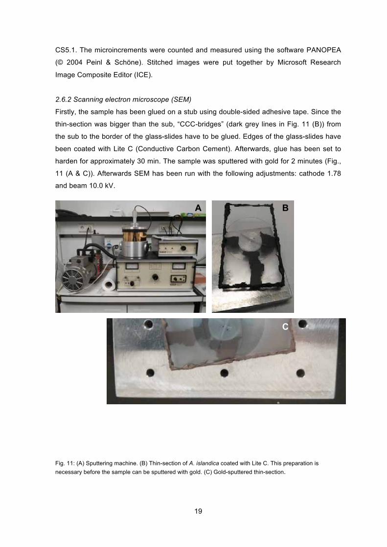
2.6.2 Scanning electron microscope (SEM)
Firstly, the sample has been glued on a stub using double-sided adhesive tape. Since the
thin-section was bigger than the sub, “CCC-bridges” (dark grey lines in Fig. 11 (B)) from
the sub to the border of the glass-slides have to be glued. Edges of the glass-slides have
been coated with Lite C (Conductive Carbon Cement). Afterwards, glue has been set to
harden for approximately 30 min. The sample was sputtered with gold for 2 minutes (Fig.,
11 (A & C)). Afterwards SEM has been run with the following adjustments: cathode 1.78
and beam 10.0 kV.
Fig. 11: (A) Sputtering machine. (B) Thin-section of A. islandica coated with Lite C. This preparation is necessary before the sample can be sputtered with gold. (C) Gold-sputtered thin-section.
C
B A
20
2.7 Thick-section preparation of bivalve shells
Thick-sections of A. islandica and Unio sp. were prepared to correlate the measured years
to calendar years. Moreover they helped to orientate in the thin-section of the same shell.
Therefore shells of both genera have been coated twice with Araldite 2020 to prepare 3
mm thick-sections. During cutting of the shell the first cut is done 3 mm right of LSG and
the second directly on LSG (Section 2.4.4). The cut thick-section is mounted with metal
epoxy resin on glass-slides, the LSG above. Additionally, they have been grinded with
sandpaper of grain size 15 µm, 10 µm and 5 µm to get a polished surface.
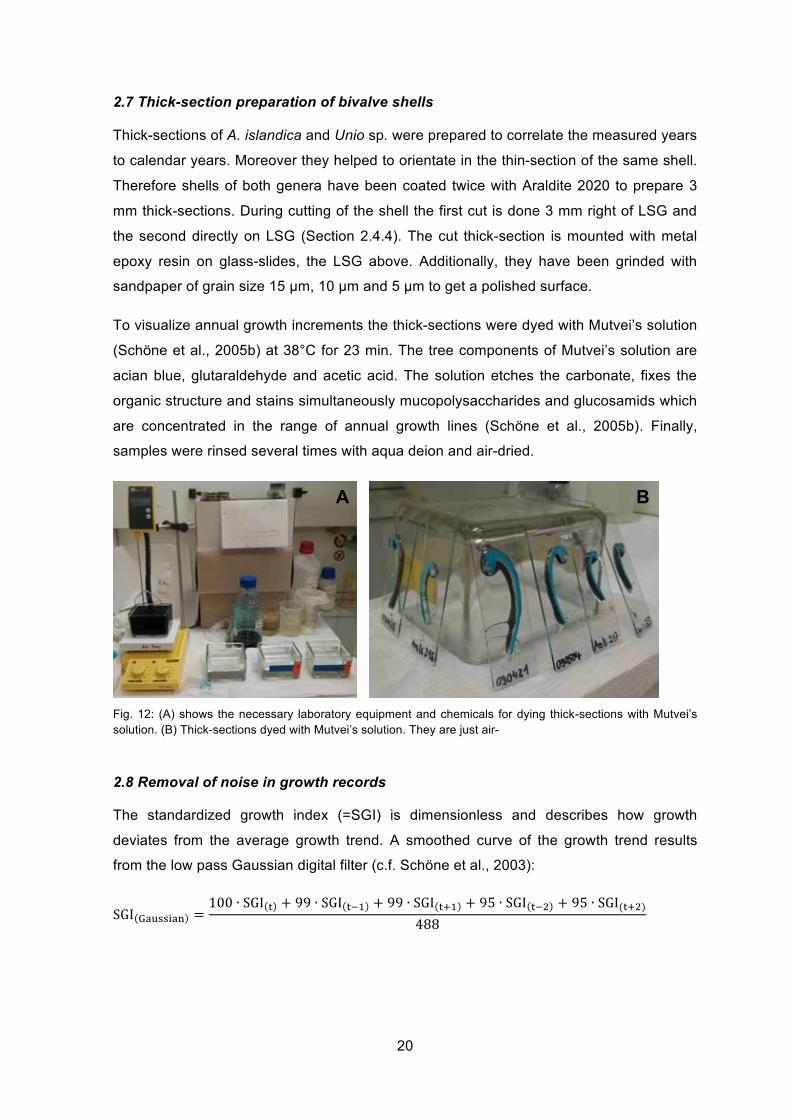
To visualize annual growth increments the thick-sections were dyed with Mutvei’s solution
(Schöne et al., 2005b) at 38°C for 23 min. The tree components of Mutvei’s solution are
acian blue, glutaraldehyde and acetic acid. The solution etches the carbonate, fixes the
organic structure and stains simultaneously mucopolysaccharides and glucosamids which
are concentrated in the range of annual growth lines (Schöne et al., 2005b). Finally,
samples were rinsed several times with aqua deion and air-dried.
Fig. 12: (A) shows the necessary laboratory equipment and chemicals for dying thick-sections with Mutvei’s solution. (B) Thick-sections dyed with Mutvei’s solution. They are just air- 2.8 Removal of noise in growth records
The standardized growth index (=SGI) is dimensionless and describes how growth
deviates from the average growth trend. A smoothed curve of the growth trend results
from the low pass Gaussian digital filter (c.f. Schöne et al., 2003):
SGI =100 ∙ SGI + 99 ∙ SGI + 99 ∙ SGI + 95 ∙ SGI + 95 ∙ SGI( )
488
A B
21
3 Results
3.1 Thin-section preparation
3.1.1 Arctica islandica
Thin-sections were prepared as described in Subsections 2.4.1-2.4.6. Other pathways
which were tried (Subsection 2.4.7) have failed. Thin-sections of fourteen A. islandica
specimens were successfully prepared and have been used to visualize microincrements.
Even though all shells were prepared in exactly the same manner, the results differ
concerning the visibility of the microincrements in some of the thin-sections. One
challenge to visualize microincrements in thin-section of A. islandica is the so called “white
band”. A white area in the outer layer of shell which is parallel to the periostracum
complicates or even prevents the measurement of microincrements.
3.1.2 Unio sp.
Two thin-sections of freshwater bivalves of Unio sp. were prepared exactly the same
pathway as shells of A. islandica (c.f. Subsection 3.1.1). Microincrements of Unio sp. are
smaller than those of the ocean quahog A. islandica.
3.2 Additional attempts to improve the visualization of microincrements
3.2.1 Etching of thin-sections with Mutvei’s solution
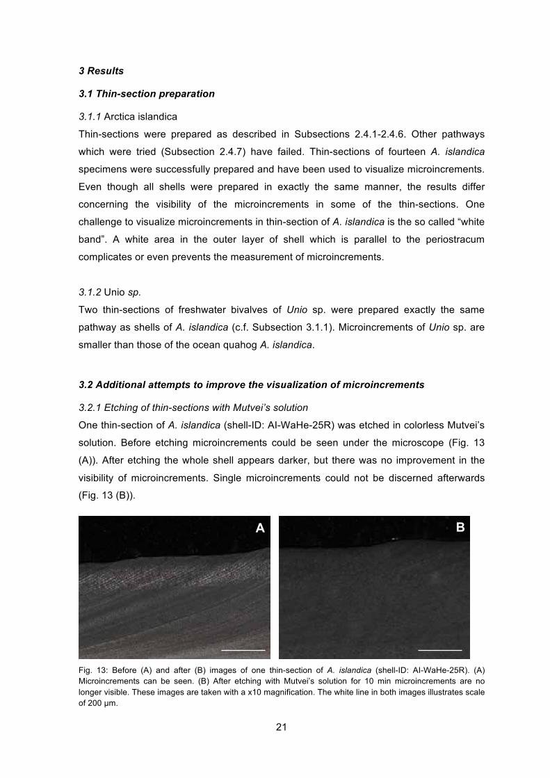
One thin-section of A. islandica (shell-ID: AI-WaHe-25R) was etched in colorless Mutvei’s
solution. Before etching microincrements could be seen under the microscope (Fig. 13
(A)). After etching the whole shell appears darker, but there was no improvement in the
visibility of microincrements. Single microincrements could not be discerned afterwards
(Fig. 13 (B)).
Fig. 13: Before (A) and after (B) images of one thin-section of A. islandica (shell-ID: AI-WaHe-25R). (A) Microincrements can be seen. (B) After etching with Mutvei’s solution for 10 min microincrements are no longer visible. These images are taken with a x10 magnification. The white line in both images illustrates scale of 200 µm.
A B B
22
3.2.2 Bleaching of thin-sections with hydrogen peroxide (H2O2)
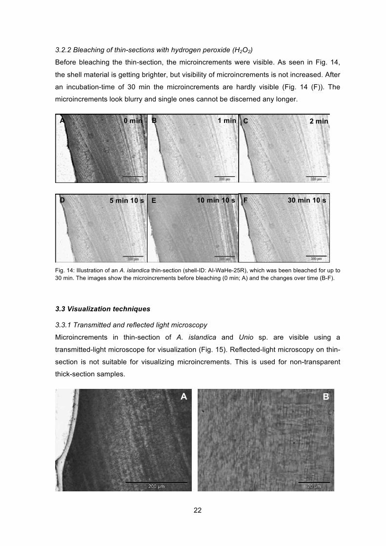
Before bleaching the thin-section, the microincrements were visible. As seen in Fig. 14,
the shell material is getting brighter, but visibility of microincrements is not increased. After
an incubation-time of 30 min the microincrements are hardly visible (Fig. 14 (F)). The
microincrements look blurry and single ones cannot be discerned any longer.
Fig. 14: Illustration of an A. islandica thin-section (shell-ID: AI-WaHe-25R), which was been bleached for up to 30 min. The images show the microincrements before bleaching (0 min; A) and the changes over time (B-F).
3.3 Visualization techniques
3.3.1 Transmitted and reflected light microscopy
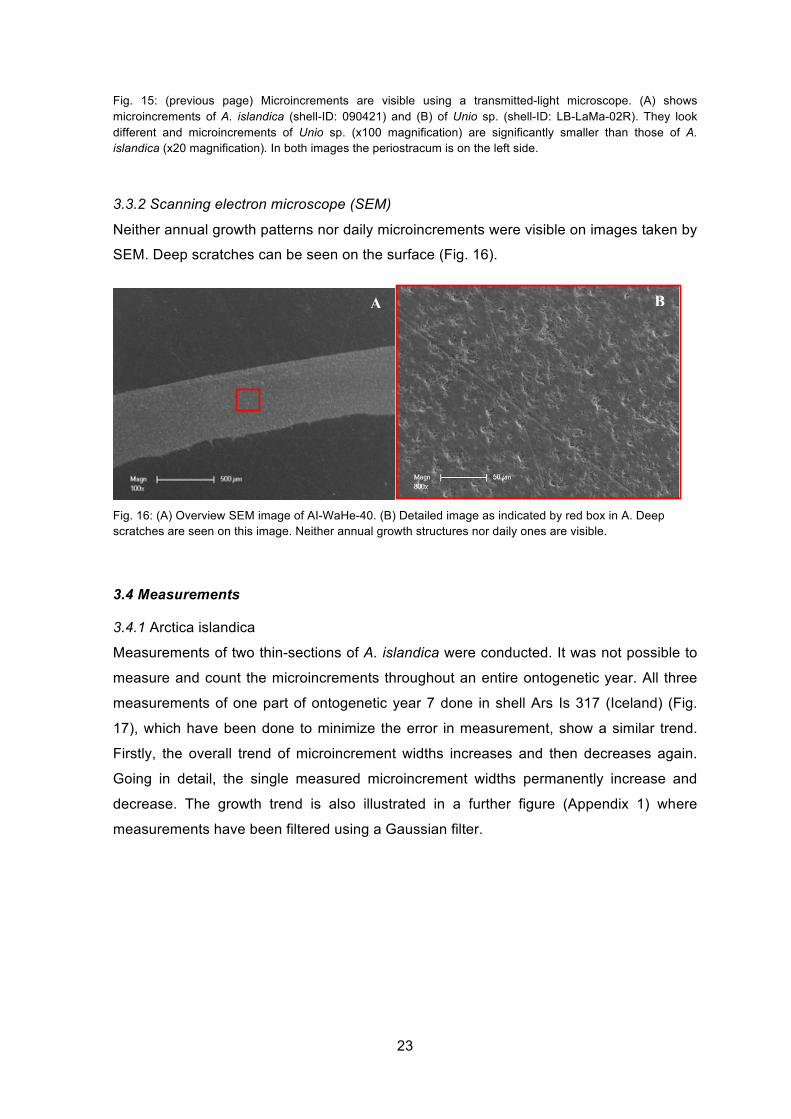
Microincrements in thin-section of A. islandica and Unio sp. are visible using a
transmitted-light microscope for visualization (Fig. 15). Reflected-light microscopy on thin-
section is not suitable for visualizing microincrements. This is used for non-transparent
thick-section samples.
0 min 1 min 2 min
5 min 10 s 10 min 10 s 30 min 10 s
A B C
D E F
A B
23
Fig. 15: (previous page) Microincrements are visible using a transmitted-light microscope. (A) shows microincrements of A. islandica (shell-ID: 090421) and (B) of Unio sp. (shell-ID: LB-LaMa-02R). They look different and microincrements of Unio sp. (x100 magnification) are significantly smaller than those of A. islandica (x20 magnification). In both images the periostracum is on the left side.
3.3.2 Scanning electron microscope (SEM)
Neither annual growth patterns nor daily microincrements were visible on images taken by
SEM. Deep scratches can be seen on the surface (Fig. 16).
Fig. 16: (A) Overview SEM image of AI-WaHe-40. (B) Detailed image as indicated by red box in A. Deep scratches are seen on this image. Neither annual growth structures nor daily ones are visible.
3.4 Measurements
3.4.1 Arctica islandica
Measurements of two thin-sections of A. islandica were conducted. It was not possible to
measure and count the microincrements throughout an entire ontogenetic year. All three
measurements of one part of ontogenetic year 7 done in shell Ars Is 317 (Iceland) (Fig.
17), which have been done to minimize the error in measurement, show a similar trend.
Firstly, the overall trend of microincrement widths increases and then decreases again.
Going in detail, the single measured microincrement widths permanently increase and
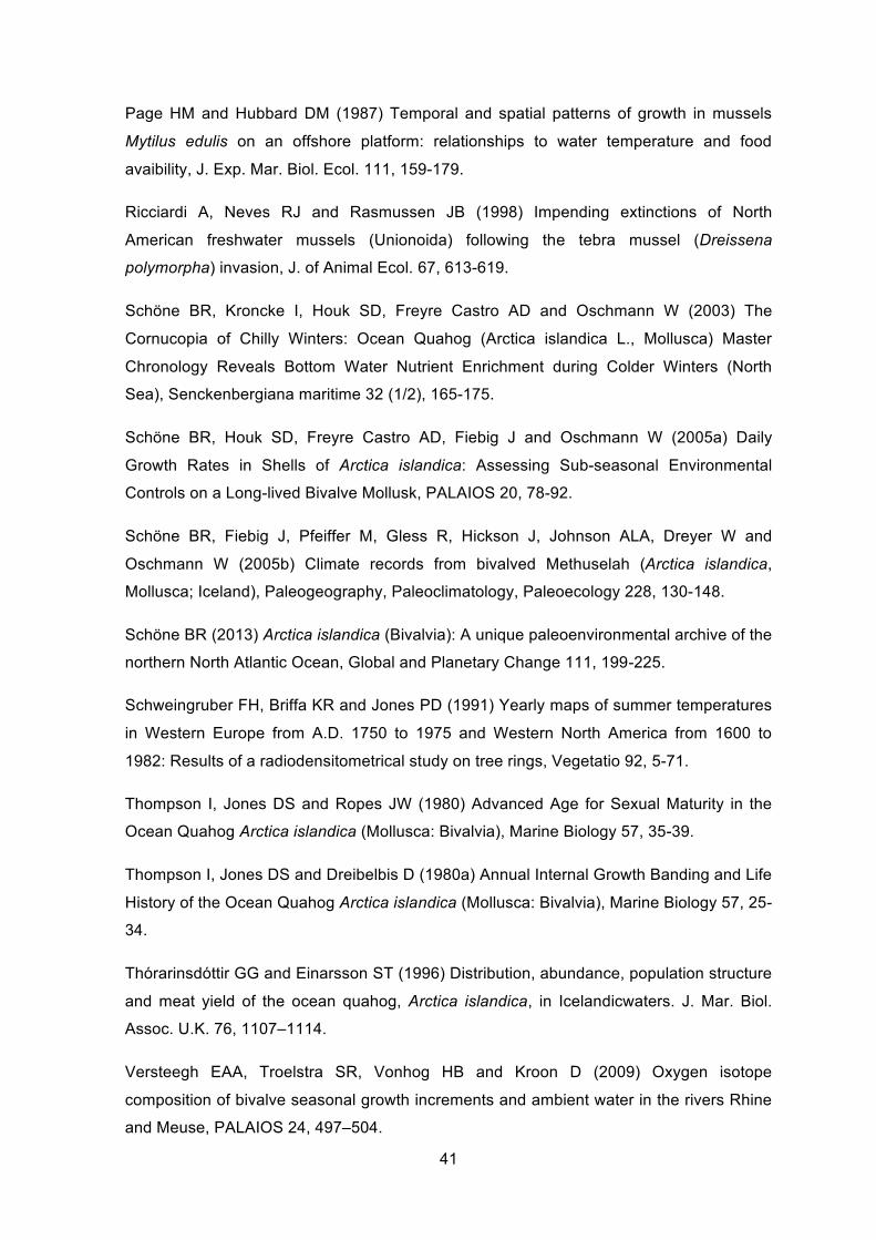
decrease. The growth trend is also illustrated in a further figure (Appendix 1) where
measurements have been filtered using a Gaussian filter.
A B
24
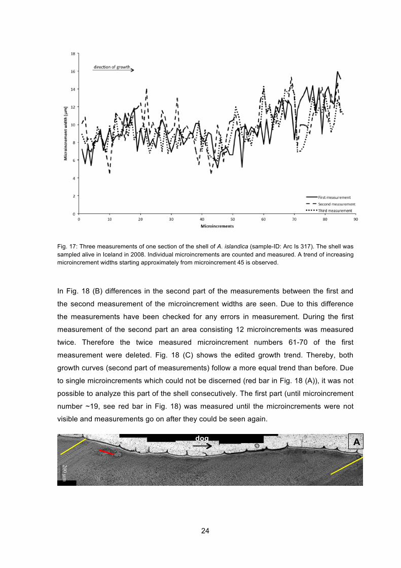
Fig. 17: Three measurements of one section of the shell of A. islandica (sample-ID: Arc Is 317). The shell was sampled alive in Iceland in 2008. Individual microincrements are counted and measured. A trend of increasing microincrement widths starting approximately from microincrement 45 is observed.
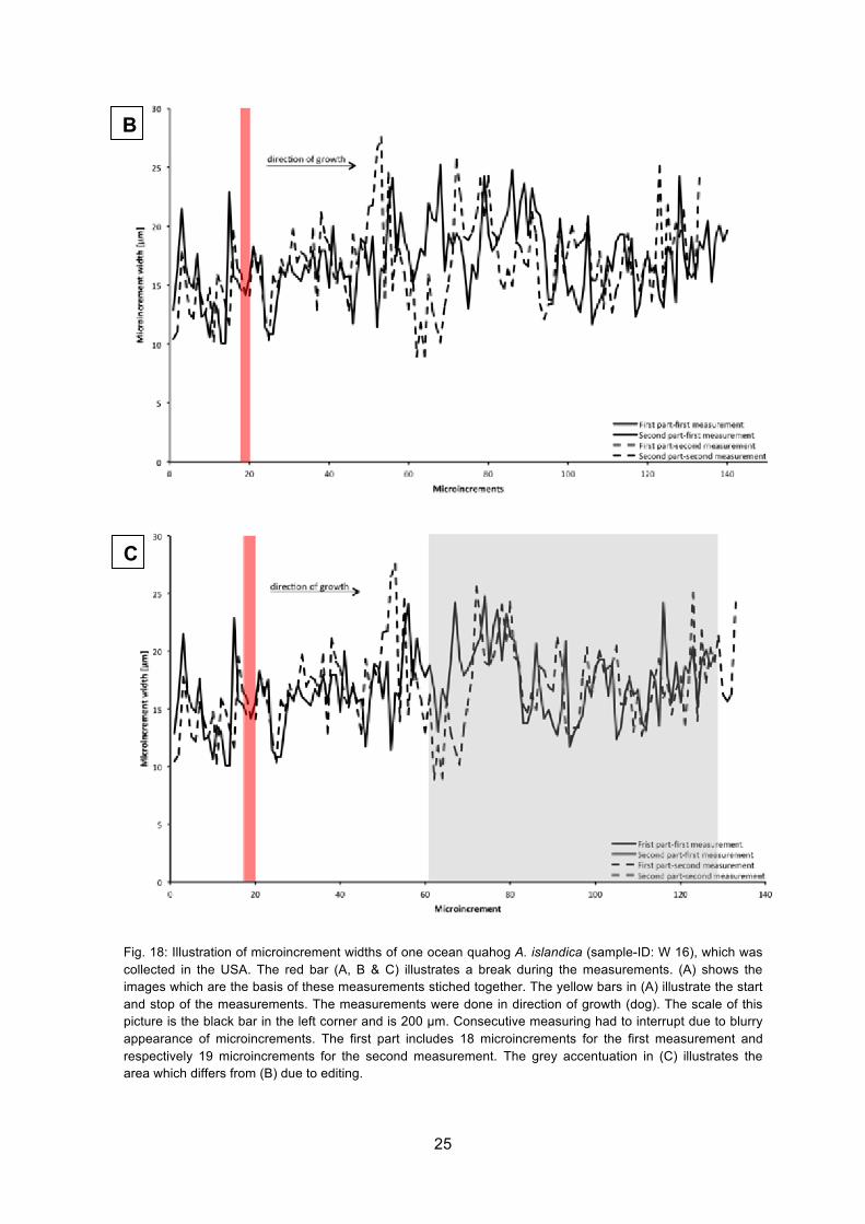
In Fig. 18 (B) differences in the second part of the measurements between the first and
the second measurement of the microincrement widths are seen. Due to this difference
the measurements have been checked for any errors in measurement. During the first
measurement of the second part an area consisting 12 microincrements was measured
twice. Therefore the twice measured microincrement numbers 61-70 of the first
measurement were deleted. Fig. 18 (C) shows the edited growth trend. Thereby, both
growth curves (second part of measurements) follow a more equal trend than before. Due
to single microincrements which could not be discerned (red bar in Fig. 18 (A)), it was not
possible to analyze this part of the shell consecutively. The first part (until microincrement
number ~19, see red bar in Fig. 18) was measured until the microincrements were not
visible and measurements go on after they could be seen again.
A dog
200 µm
25
Fig. 18: Illustration of microincrement widths of one ocean quahog A. islandica (sample-ID: W 16), which was collected in the USA. The red bar (A, B & C) illustrates a break during the measurements. (A) shows the images which are the basis of these measurements stiched together. The yellow bars in (A) illustrate the start and stop of the measurements. The measurements were done in direction of growth (dog). The scale of this picture is the black bar in the left corner and is 200 µm. Consecutive measuring had to interrupt due to blurry appearance of microincrements. The first part includes 18 microincrements for the first measurement and respectively 19 microincrements for the second measurement. The grey accentuation in (C) illustrates the area which differs from (B) due to editing.
C
B
26
3.4.2 Unio sp.
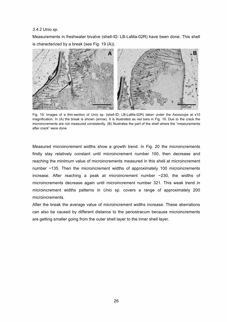
Measurements in freshwater bivalve (shell-ID: LB-LaMa-02R) have been done. This shell
is characterized by a break (see Fig. 19 (A)).
Fig. 19: Images of a thin-section of Unio sp. (shell-ID: LB-LaMa-02R) taken under the Axioscope at x10 magnification. In (A) the break is shown (arrow). It is illustrated as red bars in Fig. 19. Due to the crack the microincrements are not measured consistently. (B) Illustrates the part of the shell where the “measurements after crack” were done.
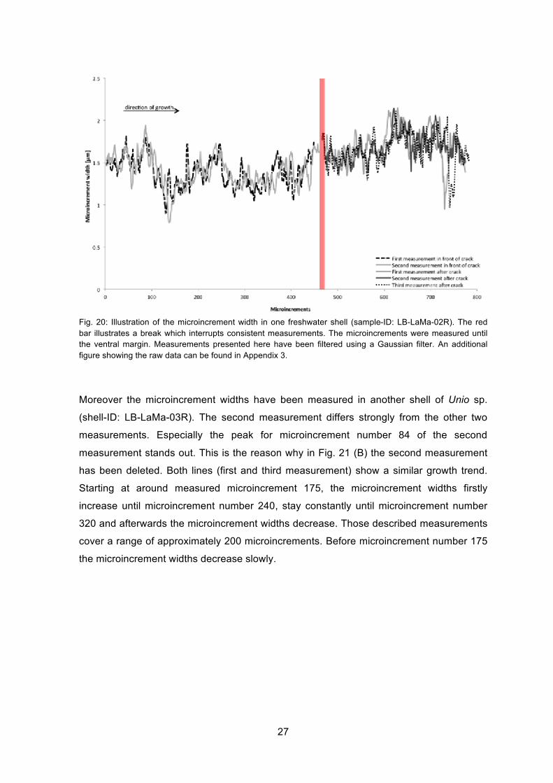
Measured microincrement widths show a growth trend. In Fig. 20 the microincrements
firstly stay relatively constant until microincrement number 100, then decrease and
reaching the minimum value of microincrements measured in this shell at microincrement
number ~135. Then the microincrement widths of approximately 100 microincrements
increase. After reaching a peak at microincrement number ~230, the widths of
microincrements decrease again until microincrement number 321. This weak trend in
microincrement widths patterns in Unio sp. covers a range of approximately 200
microincrements.
After the break the average value of microincrement widths increase. These aberrations
can also be caused by different distance to the periostracum because microincrements
are getting smaller going from the outer shell layer to the inner shell layer.
A B
27
Fig. 20: Illustration of the microincrement width in one freshwater shell (sample-ID: LB-LaMa-02R). The red bar illustrates a break which interrupts consistent measurements. The microincrements were measured until the ventral margin. Measurements presented here have been filtered using a Gaussian filter. An additional figure showing the raw data can be found in Appendix 3.
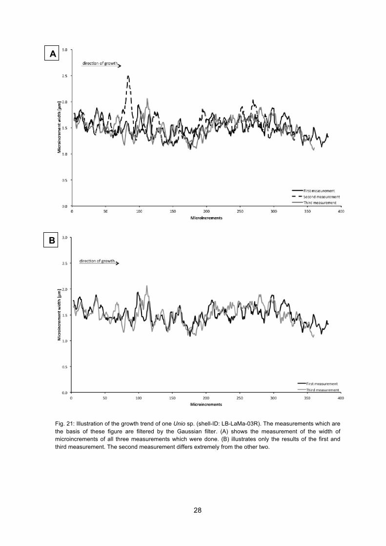
Moreover the microincrement widths have been measured in another shell of Unio sp.
(shell-ID: LB-LaMa-03R). The second measurement differs strongly from the other two
measurements. Especially the peak for microincrement number 84 of the second
measurement stands out. This is the reason why in Fig. 21 (B) the second measurement
has been deleted. Both lines (first and third measurement) show a similar growth trend.
Starting at around measured microincrement 175, the microincrement widths firstly
increase until microincrement number 240, stay constantly until microincrement number
320 and afterwards the microincrement widths decrease. Those described measurements
cover a range of approximately 200 microincrements. Before microincrement number 175
the microincrement widths decrease slowly.
28
Fig. 21: Illustration of the growth trend of one Unio sp. (shell-ID: LB-LaMa-03R). The measurements which are the basis of these figure are filtered by the Gaussian filter. (A) shows the measurement of the width of microincrements of all three measurements which were done. (B) illustrates only the results of the first and third measurement. The second measurement differs extremely from the other two.
B
A
29
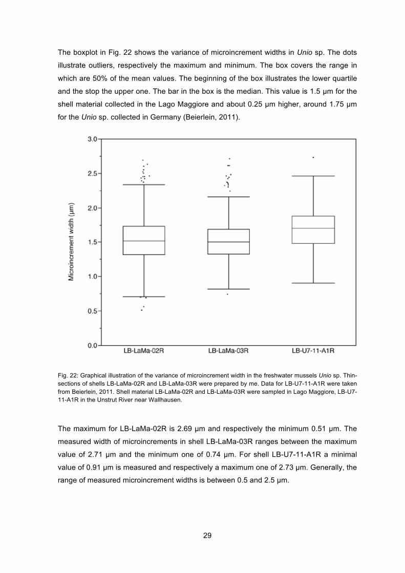
The boxplot in Fig. 22 shows the variance of microincrement widths in Unio sp. The dots
illustrate outliers, respectively the maximum and minimum. The box covers the range in
which are 50% of the mean values. The beginning of the box illustrates the lower quartile
and the stop the upper one. The bar in the box is the median. This value is 1.5 µm for the
shell material collected in the Lago Maggiore and about 0.25 µm higher, around 1.75 µm
for the Unio sp. collected in Germany (Beierlein, 2011).
Fig. 22: Graphical illustration of the variance of microincrement width in the freshwater mussels Unio sp. Thin-sections of shells LB-LaMa-02R and LB-LaMa-03R were prepared by me. Data for LB-U7-11-A1R were taken from Beierlein, 2011. Shell material LB-LaMa-02R and LB-LaMa-03R were sampled in Lago Maggiore, LB-U7-11-A1R in the Unstrut River near Wallhausen.
The maximum for LB-LaMa-02R is 2.69 µm and respectively the minimum 0.51 µm. The
measured width of microincrements in shell LB-LaMa-03R ranges between the maximum
value of 2.71 µm and the minimum one of 0.74 µm. For shell LB-U7-11-A1R a minimal
value of 0.91 µm is measured and respectively a maximum one of 2.73 µm. Generally, the
range of measured microincrement widths is between 0.5 and 2.5 µm.
30
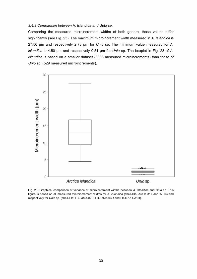
3.4.3 Comparison between A. islandica and Unio sp.
Comparing the measured microincrement widths of both genera, those values differ
significantly (see Fig. 23). The maximum microincrement width measured in A. islandica is
27.56 µm and respectively 2.73 µm for Unio sp. The minimum value measured for A.
islandica is 4.50 µm and respectively 0.51 µm for Unio sp. The boxplot in Fig. 23 of A.
islandica is based on a smaller dataset (3333 measured microincrements) than those of
Unio sp. (529 measured microincrements).
Fig. 23: Graphical comparison of variance of microincrement widths between A. islandica and Unio sp. This figure is based on all measured microincrement widths for A. islandica (shell-IDs: Arc Is 317 and W 16) and respectively for Unio sp. (shell-IDs: LB-LaMa-02R, LB-LaMa-03R and LB-U7-11-A1R).
31
4 Discussion
4.1 Thin-section preparation
Several steps are necessary to prepare thin-sections successfully: coating, cutting,
embedding, gluing on lapped glass-slides, cutting down to 200 µm and finally, lapping and
polishing. The most challenging part is the last one. Thin-sections have to be lapped down
to a thickness of approximately 30 µm. Even the supporting head of the Lapping/
Polishing machine is correctly adjusted and theoretically, the sample should not get
thinner, shell material can be lost very fast. Especially the ends of the shell often break off.
4.1.1 Arctica islandica
Microincrements in shells of A. islandica are visible using a transmitted-light microscope,
but they look blurry with increasing magnification. In none of the prepared thin-sections of
A. islandica microincrements could be seen from one winter line to the next. It is
challenging to discern between single microincrements and to measure the width of those
due to “white band” (Subsection 3.1.1). This part of the shell appears white under a
transmitted-light microscope and microincrements are hardly visible.
It is presumed that the “white band” is associated with shell structure. The “white band” is
parallel to the periostracum in the outer layer of the shell and complicates measuring of
microincrements because those are hardly visible in that part of the shell. Maybe the
organic content differs from the one at other shell parts. Working with transmitted-light the
white color point out that the shell structure is less dense than the parts of the shell
appearing darker. Moreover Araldite “penetrates” in the shell during coating. The “white
band” is not visible in thin-sections of the freshwater bivalve. But Unio sp. has a different
shell structure, which could explain why Araldite do not “penetrate” in those shells.
Furthermore the white band could be caused during lapping. If this can explain the white
area parallel to the periostracum of one shell, it would mean that this part of the shell is
more stressed during the lapping process than the rest of the shell.
At the beginning of my research, I have done several thin-sections of one shell. There are
big differences in the “quality” of thin-sections even all were prepared the same way. In all
thin-sections prepared from one shell (e.g. AI-WaHe-25R) microincrements are well or
bad visible. Therefore, in further studies more thin-sections have to be prepared than
actually needed. Those differences exist between and within populations. Intraspecific
competition explains different visibility of microincrements within one population.
32
4.1.2 Unio sp.
Using a transmitted-light microscope, microincrements are visible in thin-sections of
freshwater bivalve Unio sp. Due to different shell structure and biomineralization process
the microincrements of freshwater bivalves look completely different than those of A.
islandica. Microincrements of Unio sp. are significantly smaller than those of the ocean
quahog A. islandica (Fig. 23). A high magnification of x100 and immersion oil is necessary
to visualize, count and measured microincrements in thin-sections of Unio sp. Moreover
those thin-sections have to be perfectly lapped and polished. Any scratches degrade the
visibility of microincrements in freshwater bivalves.
4.2 Additional attempts to improve the visualization of microincrements
4.2.1 Etching of thin-section with Mutvei’s solution
The idea of etching one thin-section was to accent the microincrements. For this trial
colorless Mutvei’s solution was used. Commonly, thick-sections were colored by blue
Mutvei’s solution (Subsection 2.7). Mutvei’s solution accents the topographic relief of
growth patterns in thick-sections. This method improves the visualization of growth lines
using reflected-light microscopy. But etching thin-sections does not improve the
visualization of microincrements (Fig. 13). Those are not visible in etched thin-sections.
The visibility of microincrements in thin-sections increases the smoother the surface is.
Mutvei’s solution dissolves calcium carbonate and destroys the polished surface which is
necessary for visualization microincrements. Summing up, etching does not improve the
visibility of microincrements in bivalve shells.
4.2.2 Bleaching of thin-section with hydrogen peroxide (H2O2)
The idea of bleaching one sample was to improve the visualization of microincrements. In
contrast to etching, bleaching should accent the inter-crystalline organic matrix and bright
up the grey shadow on the shell. Some samples in total or even parts of them are very
dark which complicates the measurement of microincrements. Due to bleaching the shell
brightens up, but it does not improve the visibility of microincrements (Fig. 14). Hydrogen
peroxide reacts with calcium carbonate of the bivalve shell. The shining surface is
destroyed, but microincrements are only visible in thin-sections with perfectly polished
surfaces.
33
4.3 Visualization techniques
4.3.1 Transmitted and reflected light microscopy
Transmitted-light microscopy is used to visualize growth patterns on a daily scale.
Microincrements are visible in thin-sections of A. islandica and Unio sp. being 30-40 µm
thick (Fig. 15). Thin-sections thicker than 40 µm are too dark for the visualization of
microincrements because to less light shines through the sample. Thin-sections having a
thickness of 25 µm are too thin. Those start to polarize and microincrements are not
visible. Thin-sections thicker and thinner than the range of 30-40 µm are not suited for the
visualization of microincrements.
4.3.2 Scanning electron microscope (SEM)
No growth structures in the shell can be seen. The thin-sections were polished
(Subsection 2.4.6) to get a shining surface and removing scratches caused during cutting
and lapping, but deep scratches are visible on the SEM images (Fig. 16). Growth patterns
are not visible on the images taken by the SEM. Moreover scratches are visible even the
thin-sections were polished. The surface of this thin-section was polished, but scanning
electron microscopy works with reflected light. As described in Subsection 4.2 transmitted-
light has to be used to visualize microincrements in polished thin-sections. Therefore I
suggest using etched thin-sections to visualize growth patterns with SEM in further
studies.
4.4 Measurements
4.4.1 Arctica islandica
As described before (Subsection 3.1.1), visualizing of microincrements in marine bivalve
shell A. islandica is quite challenging. To get first information about the widths of
microincrements in this species, 90 (Arc Is 317) and respectively 130 (W 16)
microincrements were measured in two specimens, from Iceland (shell-ID: Arc Is 317) and
the USA (shell-ID: W 16).
Microincrements in A. islandica look blurry with increasing magnification. Therefore
magnifications of x10 (for Arc Is 317) and x20 (for W 16) were used to take the pictures on
which the measurements are based. As seen in Fig. 17 the minimum microincrements
widths measured in shell Arc Is 317 is 4.50 µm and respectively the maximum width is
15.94 µm for the ocean quahog collected in Iceland. The minimum value which was
measured in another shell of A. islandica (shell-ID: W16) is 8.90 µm and the maximum
value is 27.56 µm (Fig. 18). Schöne et al. (2005a) specifies the measured width of
34
microincrements in Dogger Bank (North Sea) with 6-58 µm and in the German Bight
(North Sea) with 23-51 µm. This data are based on the fourth year of growth.
The minimum and especially the maximum values measured differ from those in Dogger
Bank and German Bight. The results shown in Figs. 17 & 18 do not cover a whole year
and the microincrements were measured in different ontogenetic years. Approximately 90
(Arc Is 317) and respectively 130 (W 16) microincrements (for W 16: not consecutively)
were analyzed. In contrast, on average 232 microincrements were measured in growth
year four (Schöne et al., 2005a). Hence the measured section covers only a quarter (Arc
Is 317) and respectively the half of one year (W 16). Besides, it is not known if there is any
growth break within the measured microincrements of those shells (Arc Is 317 and W 16).
It is known that the microincrement width varies within one year (Schöne et al. 2005a).
Moreover it has to be recognized that they are from different localities with different
environmental conditions. But no conclusion concerning environment and locality could be
done due to missing information and the fact that it was not possible to measure one year
consecutively.
Figure 18 (B & C) shows the challenges measuring microincrements in marine bivalve
shells of A. islandica. As described before (Subsection 3.4.1) Fig. 18 (C) shows the edited
dataset. The grey accentuation illustrates the changes in the growth trend based on the
first measurement. This error in measurement clarifies the challenges of analyzing
microincrements in marine bivalve shells.
4.4.2 Unio sp.
A similar growth trend described for shell LB-LaMa-02R (Subsection 3.4.2, Fig. 20) can
also be seen in Fig. 21 illustrating the variance of microincrement widths in another shell
of Unio sp. (LB-LaMa-03R). In Fig. 21 this growth pattern is visible beginning at
microincrement number 175. Possibly, this point marks a (winter) annual growth line, but
those are hardly visible in thin-sections of Unio sp. The following curve covers a range of
approximately 200 microincrements as described in Beierlein (2011).
The boxplot (Fig. 22) shows that the median for both freshwater bivalves sampled in the
Lago Maggiore (shell-ID’s: LB-LaMa-02R and LB-LaMa-03R) and the Unio sp. collected in
Central Germany (shell-ID: LB-U7-11-A1R) is almost identical. The calculated medians fit
together quite well. Shells LB-LaMa-02R and LB-LaMa-03R have lived in the Lago
Maggiore in Italy, whereas Unio sp. LB-U7-11-A1R has been collected in a river in Central
Germany. The locality in Germany is further north than the Lago Maggiore in Italy.
Moreover different ontogenetic years were measured in all shells. These reasons explain
the insignificant differences in the calculated value of the median. Outliers above the

35
upper quartile can be explained by errors in measurement. Two microincrements could
not be discerned and be measured as one.
4.4.3 Comparison between A. islandica and Unio sp.
In contrast to A. islandica it is easier to visualize microincrements in shells of the
freshwater bivalve Unio sp. even the microincrements in Unio sp. are significantly smaller
than those in A. islandica (Fig. 23). The average microincrement width for A. islandica is
12.5 µm and 1.5 µm for Unio sp. Differences in biomineralization processes between
bivalve species are crucial if microincrements can be visualized.
36
5 Conclusions
In this study I focused on the preparation of thin-sections of bivalve shells and furthermore
I was interested in examining the potential of such thin-sections as a window to
environmental reconstruction on a daily scale. The main focus was on the marine species
A. islandica and the freshwater bivalve Unio sp. and finally, for both species, thin-sections
have successfully been prepared. However, during my thesis it was not possible to
correlate any environmental data to the data retrieved from the thin-sections. Main
challenge in A. islandica was the visualization of microincrements itself, whereas in Unio
sp. it was not possible to correlate environmental data due to missing information about
the date of death.
In the following the key findings of my work are summarized:
Several techniques and methods (Subsections 2.5 & 2.6) have been tested for
their potential to visualize microincrements in bivalve shell. Finally, the procedure
described in Subsections 2.4.1-2.4.6 is considered the most promising for the
preparation of thin-sections.
Microincrements can be visualized by thin-sections and they are visible in both
target species (Subsection 3.4). Microincrements in Unio sp. are significantly
smaller (1.5 µm on average) than in A. islandica (12.5 µm on average) (Fig. 23).
In A. islandica microincrements became visible using a microscope with
transmitted-light and a x10 magnification (Fig. 15). With higher magnification
microincrements looked blurry and it was not possible to measure consecutive
microincrements over an entire ontogenetic year. However, to get a first
impression about the variability in microincrement widths in A. islandica
measurements were carried out in different shell areas and different ontogenetic
years (Subsections 3.3.1 and 3.4.1, Figs. 17 and 18).
Microincrements in Unio sp. have successfully been measured consecutively.
Here, a high magnification of x100 and immersion oil were necessary to visualize,
count and measure microincrements (Subsections 3.3.1 and 3.4.2, Figs. 20 and
21).
A weak annual trend in the microincrement width pattern in Unio sp. has been
found. However, due to missing information on the date of death it was not
possible to correlate the measurements to environmental datasets (Subsections
3.4.2 and 4.4.2, Figs. 20 and 21).
37
6 Outlook
Even though the knowledge on how to successfully prepare thin-sections of bivalve shells
has been gained in this study (Subsections 2.4.1-2.4.6) further research on additional
shell material is needed in order to verify these results. Due to its exceptional importance
as a bioarchive, future work should focus on the visualization of microincrements in A.
islandica. In the following some suggestions on how to improve the visibility of
microincrements are given:
The abrasive used in this study has a grain size of 9 µm and is grey-colored.
Especially in thin-sections of A. islandica this led to a dark discoloration under the
microscope. It cannot be excluded that the abrasive “penetrated” the shell
carbonate. I suggest usage of a white-colored abrasive with an even smaller grain
size to simultaneously minimize scratches during the lapping process.
To improve the visualization of microincrements I suggest a scan using a confocal
Raman microscope. Raman maps have a high spatial resolution and can provide
information on growth patterns in biological hard parts where conventional
methods fail.
To proof if the microincrement widths differ significantly between localities further
studies have to be done. Therefore, it would be essential to measure the
microincrements in identical ontogenetic years of shells from different localities.
Shells of Unio sp. seem to be a suitable recorder of the past environment on a
daily scale. In future studies, additional thin-sections of Unio sp. shells with a
known date of death have to be prepared to visualize microincrements and
measure the microincrement widths in several years of known date (Subsections
3.4.1 and 4.4.2, Figs. 20 and 21). Knowing the date of death and the water depth
in which the bivalves have lived in, environmental datasets with a daily resolution
can be correlated with the microincrement data. This would be essential to find the
main driving factors for Unio sp. growth on a daily scale. Finally, a frequency
analysis on the measured microincrement widths could help to identify information
on reoccurring signals within the daily growth record.
38
References
Abbott RT (1974) American Seashells; The Marine Mollluska of the Atlantic and Pacific
Coasts of North America, Van Nostrand Reinhold Co., New York, pp. 663.
Arkhipkin AI (2005) Statoliths as ‘black boxes’ (life recorder) in squid, Marine and
Freshwater Research 56, 573-583.
Bauer G (1988) Threats to the Freshwater Pearl Mussel Margaritifera margaritifera L. in
Central Europe, Biological Conservation 45, 239-253.
Beierlein L (2011) High-resolution climate archives from archeological sites in Central
Germany. Diploma-Thesis, University of Mainz.
Boecker WS (2000) Abrupt climate change: causal constraints provided by the
paleoclimate record, Earth Science Review 51, 137-154.
Brey T, Arntz WE, Pauly D and Rumohr H (1990) Arctica (Cyprina) islandica in Kiel Bay
(Western Baltic): growth, production and ecological significance, J. Exp. Mar. Biol. Ecol.
136, 217-235.
Burlakova LE, Karatayevi AY and Padilla DK (2000) The Impact of Dreissena polymorpha
(PALLAS) Invasion on Unionid Bivalves, Internat. Rev. Hydrobiol. 85, 5-6, 529-541.
Butler PG, Richardson CA, Scourse JD, Wanamaker AD JR, Shammnon TM and Bennel
JD (2010) Marine climate in the Irish Sea: analysis of a 489-year marine master
chronology derived from growth increments in the shell of the clam Arctica islandica,
Quaternary Science Review 29, 1614-1632.
Cargnelli LM, Griesbach SJ, Packer DB and Weissberger E (1999) Ocean Quahog,
Arctica islandica, Life History and Habitat Characteristics, NOAA Technical Memorandum
NMFS-NE-148, Issues 122-152.
Clark GR (1975) Periodic growth and biological rhythms in experimentally grown bivalves:
in Rosenberg, GD and Runcorn SK, Eds., Growth Rhythms and the History of the Earth’s
rotation: J. Wiley and Sons, New York, p.103-117.
Davis HC and Calabrese A (1964) Combined effects of temperature and salinity on
development of eggs and growth of larvae of M. mercenaria and C. virginica, Fishery
Bulletin 63, No. 3.
39
Dettmann DL, Reische AK and Lohmann KC(1999) Controls on the stable isotope
composition of seasonal growth bands in aragonitic fresh-water bivalves (unionidae),
Geochimica et Cosmochimica Acta 63 (7/8), 1049–1057.
Dunca E, Schöne BR and Mutvei h (2005) Freshwater bivalves tell of past climates: But
how clearly do shells from polluted rivers speak?, Palaeogeography, Palaeoclimatology,
Palaeoecology 228 , 43–57.
Eiríksson J, Bartels-Jóndózzir HB, Cage AG, Gudmundsdóttir ER, Klitgaard-Kristensen D,
Marret F, Rodrigues T, Abrantes F, Austin WEN, Jiang H, Knudsen KL and Sejrup HP
(2006) Variability of the North Atlantic Current during the last 2000 years based on shelf
bottom water and sea surface temperatures along an open ocean/shallow marine transect
in Western Europe, The Holocene 16, 1017-1029.
Gillies RR, Boxb JB, Symanzikc J and Rodemarkerd EJ (2003) Effects of urbanization on
the aquatic fauna of the Line Creek watershed, Atlanta—a satellite perspective, Remote
Sensing of Environment 86, 411– 422.
Golikov AN and Scarlato OA (1973) Method for Indirectly Defining Optimum Temperatures
of Inhabitancy for Marine Cold-Blooded Animals, Marine Biology 20, 1-5.
Goodwin DH, Flessa KW, Schöne BR and Dettmann DL (2001) Cross-Calibration of Daily
Growth Increments, Stable Isotope Variation, and Temperature in the Golf of California
Bivalve Mollusk Chione cortezi: Implications for Paleoenvironmental Analysis, PALAIOS
16, 387-398.
Jiang H, Eiríksson J, Schulz M, Knudsen KL and Seidenkrantz (2005) Evidence for solar
forcing of sea-surface temperature on the North Icelandic Shelf during the late Holocene,
Geology 33, 73-76.
Jones DS (1980) Annual cycle of shell growth increment formation in two continental shelf
bivalves and its paleoecologic significance, Paleobiology 6 (3), 331-340.
Jones DS (1981) Reproductive cycles of the Atlantic surf calm Spisula solidissima, and
the ocean quahog Arctica islandica off New Jersey, Journal of Shellfish Research 1 (1),
23-32.
Jones DS, Arthur MA and Allard DJ (1989) Sclerochronological records of temperature
and growth from shells of Mercenaria mercenaria from Narragansett Bay, Rhode Island,
Mar. Biol. 102, 225-234.
40
Kennish MJ and Olsson RK (1975) Effects of thermal discharges on the microstructural
growth of Mercenaria mercenaria, Environmental Geology 1, 41-64.
Klocker CA and Strayer DL (2004) Interactions Among an Invasive Crayfish (Orconectes
rusticus), a Native Crayfish (Orconectes limosus), and Native Bivalves (Sphaeriidae and
Unionidae), Northeastern Naturalist 11 (2), 167-178.
Krause-Nehring J, Brey T and Thorrold SR (2012) Centennial records of lead
contamination in northern Atlantic bivalves (Arctica islandica), Marine Pollution Bulletin 64,
233-240.
Lutz RA, Goodsell JG, Mann R and Castagna M (1981) Experimental culture of the ocean
quahog Arctica islandica, J. World Maricul. SOC. 12(1), 196-205.
Marchitto TM Jr, Jones GA, Goddfriend GA and Weidmann CR (2000) Precise temporal
correlation of Holocene mollusk shells using sclerochronology, Quarternary Research 53,
236-246.
Marin F, Le Roy N and Marie B (2012) The formation and mineralization of mollusk shell,
Frontiers in Bioscience S4, 1099-1125.
Marwick PJ (2007) The paleogeographic and paleoclimatic significance of climate proxies
for data-model comparison. In: Mark Williams (Edt.), Deep-time Perspectives on Climate
Change: Marrying the Signal from Computer Models and Biological Proxies, Geological
Society of London, pp. 251-312.
Merill AS and Ropes JW (1969) The general distribution of the surf calm and ocean
quahog, Proceedings of the National Shellfisheries Association 69, 40-45.
Morton B (2011) The biology and functional morphology of Arctica islandica (Bivalvia:
Arcticidae) – A gerontophilic living fossil, Marine Biology Research 7, 540-553.
Murphy DB and Davidson MW (2012) Fundamentals of Light Microscopy and Electronic
Imaging, John Wiley & Sons, issue 2.
Negus CL (1966) A quantitative study of growth and production of unionid mussels in the
river Thames at reading, Journal of Animal Ecology 35, 513-532.
Nicol D (1951) MALACOLOGY-Recent species of the veneroid peleypod Arctica, Journal
of the Washington Academy of Sciences 41 (3), 102-106.
41
Page HM and Hubbard DM (1987) Temporal and spatial patterns of growth in mussels
Mytilus edulis on an offshore platform: relationships to water temperature and food
avaibility, J. Exp. Mar. Biol. Ecol. 111, 159-179.
Ricciardi A, Neves RJ and Rasmussen JB (1998) Impending extinctions of North
American freshwater mussels (Unionoida) following the tebra mussel (Dreissena
polymorpha) invasion, J. of Animal Ecol. 67, 613-619.
Schöne BR, Kroncke I, Houk SD, Freyre Castro AD and Oschmann W (2003) The
Cornucopia of Chilly Winters: Ocean Quahog (Arctica islandica L., Mollusca) Master
Chronology Reveals Bottom Water Nutrient Enrichment during Colder Winters (North
Sea), Senckenbergiana maritime 32 (1/2), 165-175.
Schöne BR, Houk SD, Freyre Castro AD, Fiebig J and Oschmann W (2005a) Daily
Growth Rates in Shells of Arctica islandica: Assessing Sub-seasonal Environmental
Controls on a Long-lived Bivalve Mollusk, PALAIOS 20, 78-92.
Schöne BR, Fiebig J, Pfeiffer M, Gless R, Hickson J, Johnson ALA, Dreyer W and
Oschmann W (2005b) Climate records from bivalved Methuselah (Arctica islandica,
Mollusca; Iceland), Paleogeography, Paleoclimatology, Paleoecology 228, 130-148.
Schöne BR (2013) Arctica islandica (Bivalvia): A unique paleoenvironmental archive of the
northern North Atlantic Ocean, Global and Planetary Change 111, 199-225.
Schweingruber FH, Briffa KR and Jones PD (1991) Yearly maps of summer temperatures
in Western Europe from A.D. 1750 to 1975 and Western North America from 1600 to
1982: Results of a radiodensitometrical study on tree rings, Vegetatio 92, 5-71.
Thompson I, Jones DS and Ropes JW (1980) Advanced Age for Sexual Maturity in the
Ocean Quahog Arctica islandica (Mollusca: Bivalvia), Marine Biology 57, 35-39.
Thompson I, Jones DS and Dreibelbis D (1980a) Annual Internal Growth Banding and Life
History of the Ocean Quahog Arctica islandica (Mollusca: Bivalvia), Marine Biology 57, 25-
34.
Thórarinsdóttir GG and Einarsson ST (1996) Distribution, abundance, population structure
and meat yield of the ocean quahog, Arctica islandica, in Icelandicwaters. J. Mar. Biol.
Assoc. U.K. 76, 1107–1114.
Versteegh EAA, Troelstra SR, Vonhog HB and Kroon D (2009) Oxygen isotope
composition of bivalve seasonal growth increments and ambient water in the rivers Rhine
and Meuse, PALAIOS 24, 497–504.
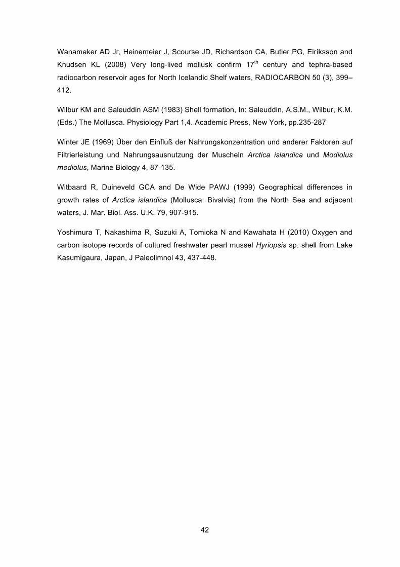
42
Wanamaker AD Jr, Heinemeier J, Scourse JD, Richardson CA, Butler PG, Eiríksson and
Knudsen KL (2008) Very long-lived mollusk confirm 17th century and tephra-based
radiocarbon reservoir ages for North Icelandic Shelf waters, RADIOCARBON 50 (3), 399–
412.
Wilbur KM and Saleuddin ASM (1983) Shell formation, In: Saleuddin, A.S.M., Wilbur, K.M.
(Eds.) The Mollusca. Physiology Part 1,4. Academic Press, New York, pp.235-287
Winter JE (1969) Über den Einfluß der Nahrungskonzentration und anderer Faktoren auf
Filtrierleistung und Nahrungsausnutzung der Muscheln Arctica islandica und Modiolus
modiolus, Marine Biology 4, 87-135.
Witbaard R, Duineveld GCA and De Wide PAWJ (1999) Geographical differences in
growth rates of Arctica islandica (Mollusca: Bivalvia) from the North Sea and adjacent
waters, J. Mar. Biol. Ass. U.K. 79, 907-915.
Yoshimura T, Nakashima R, Suzuki A, Tomioka N and Kawahata H (2010) Oxygen and
carbon isotope records of cultured freshwater pearl mussel Hyriopsis sp. shell from Lake
Kasumigaura, Japan, J Paleolimnol 43, 437-448.
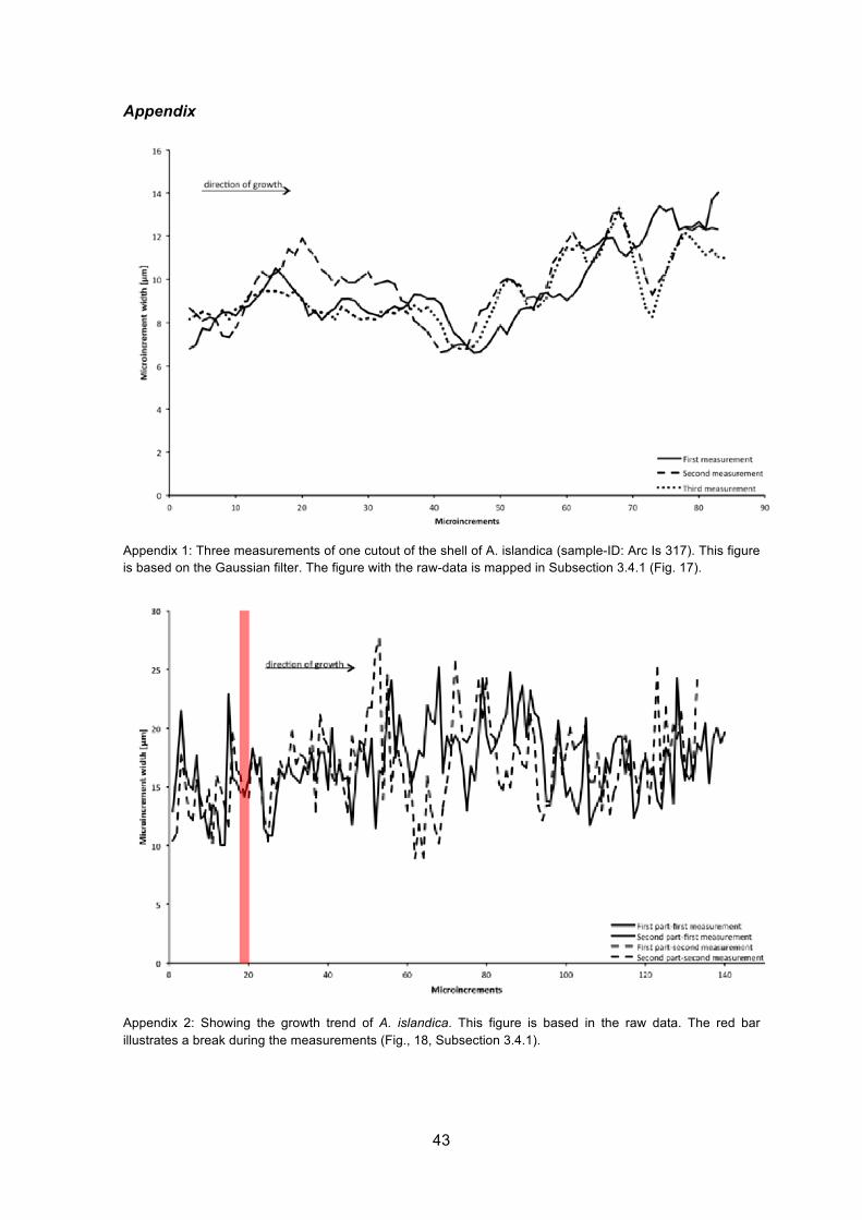
43
Appendix
Appendix 1: Three measurements of one cutout of the shell of A. islandica (sample-ID: Arc Is 317). This figure is based on the Gaussian filter. The figure with the raw-data is mapped in Subsection 3.4.1 (Fig. 17).
Appendix 2: Showing the growth trend of A. islandica. This figure is based in the raw data. The red bar illustrates a break during the measurements (Fig., 18, Subsection 3.4.1).
44
Appendix 3: Illustration of the microincrement width in one freshwater shell (sample-ID: LB-LaMa-02R). The red bar illustrates a crack which interrupts consistent measurement. The microincrements were measured until the ventral margin. This figure shows the raw data. The Gaussian filter (Fig. 20; Subsection 3.4.2) is based on this figure.


