124
TUM INSTITUT F ¨ UR INFORMATIK Workshop Petrinetze und 13. Theorietag Automaten und Formale Sprachen Markus Holzer (Herausgeber) TUM-I0322 Dezember 03 TECHNISCHE UNIVERSIT ¨ ATM ¨ UNCHEN
T U MI N S T I T U T F U R I N F O R M A T I K
Workshop Petrinetzeund
13. Theorietag Automaten und Formale Sprachen
Markus Holzer (Herausgeber)
ABCDEFGHIJKLMNOTUM-I0322
Dezember 03
T E C H N I S C H E U N I V E R S I TA T M U N C H E N
TUM-INFO-12-I0322-0/1.-FIAlle Rechte vorbehaltenNachdruck auch auszugsweise verboten
c 2003
Druck: Institut f ur Informatik derTechnischen Universit at M unchen
Vorwort
Die bisherigen Theorietage”Automaten und Formale Sprachen“ fanden in Mag-
deburg (September–Oktober 1991), Kiel (Oktober 1992), Schloß Dagstuhl (Ok-tober 1993), Herrsching bei Munchen (September 1994), Schloß Rauischholz-hausen (September 1995), Cunnersdorf bei Konigsstein (September 1996), Barn-storf bei Bremen (September–Oktober 1997), Riveres bei Trier (September 1998),Schauenburg-Elmshagen bei Kassel (September 1999), Wien (September 2000),Wendgraben bei Magdeburg (Oktober 2001) und Wittenberg (September 2002).Vom 29. September bis 2. Oktober 2003 wurde die Tradition in der Bildungstattedes Bayerischen Bauernverbandes in Herrsching bei Munchen fortgesetzt. Seitdem 6. Theorietag in Cunnersdorf wird der Theorietag von einem Workshopmit eingeladenen Vortragen begleitet. Die Themen im Laufe der Jahre lauteten:
”Perspektiven der Automaten und Formalen Sprachen“,
”Prozesse und Formale
Sprachen“,”Automaten, Formale Sprachen und Ersetzungssysteme“,
”Molecu-
lar Computing, Quantum Computing“,”Coding Theory and Formal Languages“
und”Berechenbarkeit und Komplexitat in der Analysis“. Das diesjahrige Thema
des Workshops lautet”Petrinetze“. Es nahmen 29 TeilnehmerInnen aus Australi-
en, Deutschland, Frankreich, Kanada, Osterreich, Schweden und Tschechien teil.Das wissenschaftliche Programm bestand aus angemeldeten und eingeladenenBeitragen der TeilnehmerInnen. Die Kurzzusammenfassungen der Beitrage sindin diesem Bericht abgedruckt.
Ich danke allen TeilnehmerInnen fur ihre interessanten Beitrage und die Be-reitschaft zur wissenschaftlichen Diskussion. Ich danke auch der Technischen Uni-versitat Munchen, insbesondere Herrn Brauer, fur ihre Unterstutzung und al-len MitarbeiterInnen der Bildungsstatte des Bayerischen Bauernverbandes Herr-sching fur ihren Einsatz vor und wahrend der Tagung. Ohne ihre organisato-rische Hilfe ware das Treffen nicht moglich gewesen. Auch ein recht herzlichesDankeschon an die HUK-Coburg AG fur die Sachspenden zum Theorietag. Demnachsten Theorietag in Caputh bei Potsdam wunsche ich viel Erfolg.
Ein besonderer Dank gilt Frau Erika Leber fur die hilfreiche Unterstutzung beider Organisation des Theorietags und Bernd Reichel fur die Email-Unterstutzungund das Korrekturlesen der HTML-Seiten.
Garching, im September 2003 Markus Holzer

Inhaltsverzeichnis
Vortragsprogramm 5
Zusammenfassungen der eingeladenen Vortrage 9Eike Best, Sprach- und Pomset-Aquivalenz bei beschrifteten Petrinetzen 9Javier Esparza, Some applications of Petri nets to the verification of
parametrized systems . . . . . . . . . . . . . . . . . . . . . . . . . 10Ekkart Kindler, Uber den zweckmaßigen Einsatz von Petrinetzen . . . . 12Karsten Schmidt, Supporting explicit state space verification by transi-
tion invariants . . . . . . . . . . . . . . . . . . . . . . . . . . . . . 13
Zusammenfassungen der eingereichten Vortrage 15Suna Bensch and Maia Hoeberechts, On the degree of nondeterminism
of tree adjoining languages and head grammar languages . . . . . 15Henning Bordihn and Henning Fernau, The degree of parallelism . . . . 19Henning Fernau, Formal language aspects of identifiable language classes 27Rudolf Freund, Marion Oswald und Ludwig Staiger, P-Automaten und
ω-P-Automaten . . . . . . . . . . . . . . . . . . . . . . . . . . . . 35Jens Glockler, Uber mehrdimensionale Rebound-Automaten . . . . . . . 48Martin Beaudry, Jose M. Fernandez, and Markus Holzer, A common
algebraic characterization of probabilistic and quantum computations 51Daniel Kirsten, Distance automata and the star height problem . . . . . 54Markus Holzer, Andreas Klein, and Martin Kutrib, On the NP-completeness
of the Nurikabe puzzle and variants thereof . . . . . . . . . . . . 57Roman Konig, Eine kombinatorische Eigenschaft gewisser 0, 1-Matrizen 59Martin Kutrib,On the descriptional power of heads, counters, and pebbles 63Martin Lange, Verification of non-regular properties . . . . . . . . . . . 66Benedikt Bollig and Martin Leucker, A hierarchy of MSC languages . . 73Andreas Malcher, Minimizing finite automata is computationally hard . 78Frantisek Mraz and Friedrich Otto, Hierarchies of weakly monotone re-
starting automata . . . . . . . . . . . . . . . . . . . . . . . . . . . 83Martin Platek, Marketa Lopatkova, and Karle Oliva, Restarting auto-
mata: motivations and applications . . . . . . . . . . . . . . . . . 90
3
Klaus Reinhardt, Some more regular languages that are Church Rossercongruential . . . . . . . . . . . . . . . . . . . . . . . . . . . . . . 97
Cristian S. Calude and Ludwig Staiger, Relativisations of disjunctiveness102Ralf Stiebe, On the size of hybrid networks of evolutionary processors . 110
GI-Fachgruppe 0.1.5.”Automaten und Formale Sprachen“ 113
Wahl der Fachgruppenleitung . . . . . . . . . . . . . . . . . . . . . . . 113Wahl des Fachgruppensprechers . . . . . . . . . . . . . . . . . . . . . . 114
TeilnehmerInnenliste 115
4

Vortragsprogramm
Dienstag, der 30. September 2003
9:15–9:20 Begrußung der TeilnehmerInnen zum Workshop”Petrinetze“
9:20–10:25 Eike Best, Sprach- und Pomset-Aquivalenz bei beschrifteten Petri-netzen
10:25–10:55 Kaffeepause
10:55–12:00 Ekkart Kindler, Uber den zweckmaßigen Einsatz von Petrinetzen
12:00–14:00 Mittagspause
14:00–15:05 Karsten Schmidt, Supporting explicit state space verification bytransition invariants
15:05–15:40 Kaffeepause
15:40–16:45 Javier Esparza, Some applications of Petri nets to the verificationof parametrized systems
5
Mittwoch, der 1. Oktober 2003
8:55–9:00 Begrußung der TeilnehmerInnen zum Theorietag
9:00–9:25 Henning Bordihn, The degree of parallelism
9:25–9:50 Maia Hoeberechts, On the degree of nondeterminism of tree adjoininglanguages and head grammar languages
9:50–10:15 Andreas Malcher, Minimizing finite automata is computationallyhard
10:15–10:40 Roman Konig, Eine kombinatorische Eigenschaft gewisser 0, 1-Matrizen
10:40–11:10 Kaffeepause
11:10–11:35 Daniel Kirsten, Distance automata and the star height problem
11:35–12:00 Martin Lange, Verification of non-regular properties
12:00–12:25 Martin Leucker, A hierarchy of MSC languages
12:25–14:00 Mittagspause
14:00–14:25 Martin Kutrib, On the descriptional power of heads, counters, andpebbles
14:25–14:50 Jens Glockler, Uber mehrdimensionale Rebound-Automaten
14:50–15:15 Markus Holzer, A common algebraic characterization of probabili-stic and quantum computations
15:15–15:45 Kaffeepause
15:45–16:10 Martin Platek, Restarting automata: motivations and applications
16:10–16:35 Frantisek Mraz, Hierarchies of weakly monotone restarting auto-mata
16:35–17:00 Klaus Reinhardt, Some more regular languages that are ChurchRosser congruential
17:00–18:00 Vollversammlung der GI Fachgruppe 0.1.5
6

Donnerstag, der 2. Oktober 2003
9:00–9:25 Henning Fernau, Formal language aspects of identifiable language clas-ses
9:25–9:50 Andreas Klein, On the NP-completeness of the Nurikabe puzzle andvariants thereof
9:50–10:15 Ludwig Staiger, Relativisations of disjunctiveness
10:15–10:45 Kaffeepause
10:45–11:10 Marion Oswald, P-Automaten
11:10–11:35 Rudolf Freund, ω-P-Automaten
11:35–12:00 Ralf Stiebe, On the size of hybrid networks of evolutionary proces-sors
12:00– Mittagspause und Abreise
7

8
SPRACH- UND POMSET-AQUIVALENZ BEIBESCHRIFTETEN PETRINETZEN
Eike Best
Universitat Oldenburg, Fakultat IIDepartment fur Informatik, 26111 Oldenburg, Germany
e-mail: [email protected]
KURZFASSUNG
Wir analysieren, welche Transformationen das Sprach- bzw. das Pomsetverhal-ten eines Petrinetzes invariant lassen. Es werden drei neuere Resultate und eineVermutung vorgestellt:
• Jedes k-beschrankte beschriftete Petrinetz lasst sich in ein pomset-aquivalentes 1-beschranktes Petrinetz transformieren (Best/Wimmel 2000).
• Jeder k-beschrankte Synchronisationsgraph lasst sich in einen sprach-aquivalenten 1-beschrankten Synchronisationsgraphen transformieren; esgibt jedoch einen 2-beschrankten Synchronisationsgraphen, der keinpomset-aquivalentes 1-beschranktes Pendant (Synchronisationsgraph) be-sitzt (Darondeau/Wimmel 2002).
• Jeder 1-beschrankte Synchronisationsgraph mit stillen Transitionen τ lasstsich in einen pomset-aquivalenten 1-beschrnkten Synchronisationsgraphenohne τ -Transitionen transformieren (Wimmel/Best 2003).
• Vermutung: die Beschrankung auf Synchronisationsgraphen kann im letztenSatz weggelassen werden.
9

SOME APPLICATIONS OF PETRI NETS TO THEVERIFICATION OF PARAMETRIZED SYSTEMS
Javier Esparza
Institut fur Formale Methoden der InformatikUniversitat Stuttgart, Universitatstr. 38
70569 Stuttgart, Germanye-mail: [email protected]
ABSTRACT
Many systems are designed to work for different values of a parameter. Forinstance, a carry look-ahead adder should work correctly for binary numbersof arbitrary length (it is then instantiated as a 32-bit, 64-bit adder etc.); multi-cast communication protocols should work for arbitrary numbers or receivers androuters; cryptographic protocols should be secure independently of the numberof principals that use the protocol; a cahe coherence protocol should work forarbitrarily many caches. In all these cases, the verification task consists of prov-ing that all members of an infinite family of systems, obtained by instantiatingparameters with different values, behave correctly.
Petri net analysis techniques (more precisely, techniques for place/transitionnets) have proved successful in attacking this problem when the parameter cor-responds to the number of processes or active components of the system, andwhen these components have identical (or at least very similar) structure. Themain idea is to interpret the places of the net as the possible local states of onecomponent, and interpret the number of tokens on the place as the number ofcomponents that are currently in that state. This approach was first proposed byGerman and Sistla in [6]. They used coverability trees a la Karp-Miller to deriveanalysis algorithms. Another important milestone was the discovery of a surpris-ingly simple backwards reachability technique by Abdulla, Cerans, Jonsson, andTsay [1].
One of the limitations of place/transition nets in the context of parametrizedverification is the fact that they can only model communication by rendezvous:two processes (or, more generally, an arbitrary but fixed number of processes)
10
Some applications of Petri nets to the verification of parametrized systems 11
synchronize and change their states, while all other processes remain idle. Thereis no possibility to model broadcast communication, in which a process sends amessage to all others, independently of how many they are (their number canchange dynamically when process creation is allowed). Extensions of the anal-ysis techniques to these cases have been studied by a number of people, see forinstance [2, 3, 4, 5].
In the talk I will present the main analysis techniques together with somenegative results that outline the limitations of the approach.
References
[1] Parosh Aziz Abdulla, Karlis Cerans, Bengt Jonsson, Yih-Kuen Tsay: Algo-rithmic Analysis of Programs with Well Quasi-ordered Domains. Informationand Computation 160(1-2): 109-127 (2000)
[2] Giorgio Delzanno, Jean-Franois Raskin, Laurent Van Begin: Towards theAutomated Verification of Multithreaded Java Programs. TACAS 2002: 173-187
[3] Giorgio Delzanno, Javier Esparza, Andreas Podelski: Constraint-BasedAnalysis of Broadcast Protocols. CSL 1999: 50-66
[4] Catherine Dufourd, Alain Finkel, Ph. Schnoebelen: Reset Nets BetweenDecidability and Undecidability. ICALP 1998: 103-115
[5] Javier Esparza, Alain Finkel, Richard Mayr: On the Verification of BroadcastProtocols. LICS 1999: 352-359
[6] Steven M. German, A. Prasad Sistla: Reasoning about Systems with ManyProcesses. JACM 39(3): 675-735 (1992)
UBER DEN ZWECKMASSIGEN EINSATZ VONPETRINETZEN
Ekkart Kindler
Institut fur Informatik, Universitat PaderbornWarburger Straße 100, 33098 Paderborn, Germany
e-mail: [email protected]
KURZFASSUNG
Petrinetze sind ein Formalismus – genauer eine Familie verwandter Formalis-men – zur Modellierung des Verhaltens reaktiver und verteilter Systeme. DiePetrinetztheorie bietet viele verschiedene Techniken, um Aussagen uber verschie-dene Aspekte des modellierten Systems und seines Verhaltens zu treffen.
Da Petrinetze ein sehr allgemeiner und elementarer Formalismus sind, lassensich Petrinetze in vielen verschiedenen Anwendungsgebieten, fur viele verschie-dene Anwendungszwecke und auf verschiedenen Abstraktionsebenen einsetzen.Je nach Gebiet und Zweck werden Petrinetze auf sehr unterschiedliche Weise zurModellierung, Analyse und Validierung eingesetzt. Dementsprechend gibt es vieleverschiedene Modellierungsparagdigmen fur Petrinetze.
Im Vortrag werden anhand einiger Beispiele verschiedene Modellierungspara-digmen diskutiert. Außerdem wird gezeigt, wie verschiedene Aspekte des System-verhaltens durch geeignete Erganzungen des Petrinetzmodells unabhangig von-einander untersucht werden konnen. Als Beispiele betrachten wir die Modellie-rung von Algorithmen bzw. von
”algorithmischen Ideen“, die Modellierung von
Geschaftsprozessen und die Modellierung von Materialflußsystemen.
12
SUPPORTING EXPLICIT STATE SPACEVERIFICATION BY TRANSITION INVARIANTS
Karsten Schmidt
Institut fur Informatik, Humboldt-Universitat zu BerlinUnter den Linden 6, 10099 Berlin, Germanye-mail: [email protected]
ABSTRACT
Traditionally, Petri net invariants are applied as a tool to replace state spaceverification. They are characterized as solutions of a linear system of equationsderived from the incidence matrix of the given Petri net and can thus be easilycomputed.
In this talk, we present three examples that show how one kind of invariants—transition invariants–can be used to support state space verification. In all exam-ples, we exploit the well known fact that transition invariants are closely relatedto cycles in the state space: if a transition sequence forms a cycle then the vec-tor counting the occurrences of transitions in this sequence forms a transitioninvariant. Algebraically, a transition invariant is a linear combination of transi-tion vectors that generate the 0 vector. From studying the system of equationsdefining transition invariants, we can partition the set of transitions into a set Uand a set U where the set U contains a set of linear independent transitions ofmaximum size (that size is given by the rank of the incidence matrix) and theset U of all remaining transitions. Consequently,
• A sequence of transitions from U does not form cycles, or, rephrased:
• Every cycle in the state space contains an element of U .
Exactly this information is applied in the following three scenarios.First scenario (already presented at TACAS 2003). The purpose of storing
states permanently in explicit state space verification is termination (throughassuring that one and the same state is not explored twice). It has been observedthat this condition can be weakened to: assure that on every cycle in the statespace there is a state that is not explored twice (so it is sufficient to store only
13
14 K. Schmidt
those states permanently). The remaining states are re-explored upon every visit.In our approach, we store those states permanently where a transition from U isfired and cover therefore all cycles.. We show that, at least in connection withpartial order reduction and a simple heuristic add-on, this method turns out tobe quite useful.
Second scenario. One of the most important reduction techniques in explicitstate space verification is partial order reduction. It works by exploring, in everystate, only a subset of the enabled transitions. This subset satisfies a numberof criteria in order to assure that the reduced state space holds the examinedproperty if and only if the full state space does. Among the criteria are some thatcan be computed directly from the current state and the system structure. Yetthere are other criteria requiring that some transitions must occur at least once onevery cycle in the reduced system. Traditionally, these criteria are implementedusing depth first search (then, every cycle contains a state that has, while visited,a successor on the depth first search stack). This implementation depends on astrictly sequential exploration of the state space. In distributed verification, it isnot as easy to detect cycles. We propose to use the the same structural criterionas in the first scenario: If something needs to be done at least once on every cycle,do it whenever a transition of U is fired. This approximation leads to acceptableresults.
Third scenario. The sweep-line method, recently introduced, is about remov-ing previously computed states as soon as they are no longer possible successorsof unexplored states. A progress measure (an assignment of a number to eachstate— in its basic shape monotonous w.r.t. the successor relation) gives thenecessary information: remove states that have smaller progress values than theunexplored states. The method has been generalized to non-monotonous progressmeasures. Whenever a state has a smaller progress value than its predecessor, itis stored permanently, and is used as the starting point of another state spaceexploration. The crucial tool in this method is a suitable progress measure (onewhere only few transitions decrease progress values). In the original papers, con-struction of a progress measure is left to the user. We propose the followingautomated construction of a progress measure. Let the initial state have progressvalue 0. Let every transition in U cause an increase of the measure by 1. Theincrease or decrease of the remaining transitions can be determined by the factthat all of them can be expressed as linear combinations of the transitions inU . This way, we obtain a sound (not necessarily monotonous) progress measurethat—when applied in combination with partial order reduction—leads to sig-nificant reduction even for reactive systems with a lot of local cycles (where onewould not immediately expect a notion of ”progress”).
Transition invariants turn out to be a nice tool for very different applicationsin explicit state space verification. We assume that there are more applicationareas pending.

ON THE DEGREE OF NONDETERMINISM OF TREE
ADJOINING LANGUAGES AND HEAD GRAMMARLANGUAGES
Suna Bensch
Institut fur Informatik, Universitat PotsdamAugust-Bebel-Str. 89, 14482 Potsdam, Germany
e-mail: [email protected]
and
Maia Hoeberechts
Department of Computer ScienceUniversity of Western Ontario, N6A 5B7
London, Ontario, Canadae-mail: [email protected]
ABSTRACT
The degree of nondeterminism is a measure of syntactic complexity which was in-vestigated for parallel rewriting systems as well as for sequential rewriting systems.In this paper, we consider the degree of nondeterminsm for tree adjoining gram-mars and their languages and head grammars and their languages. We show thata degree of nondeterminism of 2 suffices for both formalisms in order to generateall languages in their respective language families. Furthermore, we show that de-terministic tree adjoining grammars (those with degree of nondeterminism equalto 1), can generate non-context-free languages, in contrast to deterministic headgrammars which can only generate languages containing a single word.
Keywords: Syntactic complexity, degree of nondeterminism, tree adjoining gram-mars, head grammars.
1. Introduction
The degree of nondeterminism for tabled Lindenmayer systems and languages hasbeen studied in [11, 10] as a measure of syntactic complexity. The degree of non-determinism has also been considered for sequential rewriting systems [1, 2, 3].The degree of nondeterminism is usually defined as the maximal number of pro-duction rules with the same left-hand side. In this paper we consider the degree of
15
16 S. Bensch, M. Hoeberechts
nondeterminism for tree adjoining grammars and head grammars. Tree adjoininggrammars (TAG for short) were first introduced in [5] and further investigatedin [12, 6, 8, 7]. TAGs are tree-generating grammars which use an adjoining op-eration that generates new trees by joining and attaching two different trees ata particular node. Head Grammars (HG for short) were first introduced by Pol-lard in his PhD Thesis [9]. The principle feature which distinguishes a HeadGrammar from a context-free grammar is that the head grammar includes awrapping operation which allows one string to be inserted into another string ata specific point (the head). It is known that for both tree adjoining grammarsand head grammars, the class of string languages generated by the grammar islarger than the class of context-free languages — for example, they are able todefine the language anbncndn [12]. In [12] it is shown that the two formalismsgenerate exactly the same class of string languages, and that these languages aremildly-context-sensitive [12, 7, 6].
2. Degree of Nondeterminism for TAGs and HGs
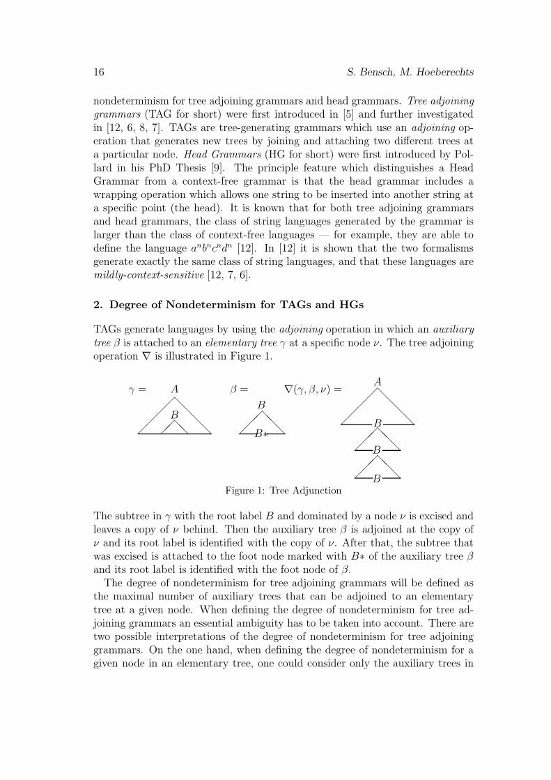
TAGs generate languages by using the adjoining operation in which an auxiliarytree β is attached to an elementary tree γ at a specific node ν. The tree adjoiningoperation ∇ is illustrated in Figure 1.
γ = β = ∇(γ, β, ν) =
��
��
A
@@
@@
��B
@@ ���B
@@@
B∗�
��
�
@@
@@A
B
���
@@@
B
���
@@@
BFigure 1: Tree Adjunction
The subtree in γ with the root label B and dominated by a node ν is excised andleaves a copy of ν behind. Then the auxiliary tree β is adjoined at the copy ofν and its root label is identified with the copy of ν. After that, the subtree thatwas excised is attached to the foot node marked with B∗ of the auxiliary tree βand its root label is identified with the foot node of β.
The degree of nondeterminism for tree adjoining grammars will be defined asthe maximal number of auxiliary trees that can be adjoined to an elementarytree at a given node. When defining the degree of nondeterminism for tree ad-joining grammars an essential ambiguity has to be taken into account. There aretwo possible interpretations of the degree of nondeterminism for tree adjoininggrammars. On the one hand, when defining the degree of nondeterminism for agiven node in an elementary tree, one could consider only the auxiliary trees in
Degree of nondeterminism of TAGs and HGs 17
the set SA which is a set that specifies all auxiliary trees that can be adjoinedat that node. On the other hand, one could consider all auxiliary trees for thegiven tree adjoining grammar (even if they are not in the set SA). We will callthese views weak degree of nondeterminism and strong degree of nondeterminismrespectively, and we show that the two measures are equivalent.
Head grammars were first introduced by Pollard in his PhD Thesis [9] and werecompared with tree adjoining grammars in [13]. In a head grammar, a specialposition between two symbols, marked by ↑, is designated as the split point ofa string. The split point is the location at which one string can be inserted intoanother during a wrapping operation. Intuitively, the degree of nondeterminismfor head grammars will measure how much choice between productions rules thereis when doing a derivation using a specific head grammar.
We show for TAGs and their languages and for HGs and their languages
1. that one can reduce the degree of nondeterminism of a TAG G to 2,
2. that one can reduce the degree of nondeterminism of a HG G to 2, and
3. that tree adjoining grammars with degree of nondeterminism 1 (determin-istic tree adjoining grammars) can generate non-context-free languages incontrast to deterministic head grammars which can only generate languagescontaining a single word
References
[1] H. Bordihn, Uber den Determiniertheitsgrad reiner Versionen formalerSprachen. PhD thesis, Technische Universitat “Otto von Guericke” Magde-burg, 1992.
[2] H. Bordihn, On The Degree Of Nondeterminism. In: Developments in The-oretical +Computer Science (1994), 133–140.
[3] H. Bordihn, S. Aydin, Sequential versus parallel grammar formalisms withrespect to measures of descriptional complexity. To appear in FundamentaInformaticae 2003.
[4] F. Gecseg, M. Steinby, Tree Languages. In G. Rozenberg, A. Salomaa (eds.),Handbook of Formal Languages, vol. 3, Springer, 1997.
[5] A. K. Joshi, L. S. Levi, M. Takahashi, Tree adjunct grammars. J. Comput.System Sci. 10 (1975), 136–163.
[6] A. K. Joshi, How much context-sensitivity is necessary for characterizingstructural descriptions: Tree adjoining grammars. In D. Dowty, L. Kart-tunen, and A. Zwicky, eds., Natural Language Parsing: Psychological, Com-putational and Theoretical Perspectives. Cambridge University Press, NewYork, 1985.
18 S. Bensch, M. Hoeberechts
[7] A. K. Joshi, K. Vijay-Shanker, D. J. Weir, The convergence of mildly context-sensitive grammar formalism. In P. Sells, S. M. Shieber, and Th. Wasow(eds), Foundational Issues in Natural Languuage Processing, MIT Press,Cambridge, 1991.
[8] A. K. Joshi, Y. Schabes, Tree adjoining grammars. In G. Rozenberg, A.Salomaa (eds.), Handbook of Formal Languages, vol. 3, Springer, 1997.
[9] C. Pollard, Generalized Phrase Structure Grammars, Head Grammars andNatural Language. PhD thesis, Stanford University, 1984.
[10] G. Rozenberg, Extension of tabled 0L systems and languages. Int. J. ofComputer and information sciences 2 (1973), 311–335.
[11] G. Rozenberg, TOL systems and languages. Information and Control 23(1973), 357–381.
[12] K. Vijay-Shanker, D. J. Weir, The equivalence of four extensions of context-free grammars. Mathematical Systems Theory 87 (1994), 511–546.
[13] D. J. Weir, K. Vijay-Shanker, A. K. Joshi, The relationship between treeadjoining grammars and head grammars. In Proceedings of the 24th AnnualMeeting of Computational Linguistics, New York, NY, June 1986.
THE DEGREE OF PARALLELISM
Henning Bordihn
Institut fur Informatik, Universitat PotsdamAugust-Bebel-Straße 89, D-14482 Potsdam, Germany
e-mail: [email protected]
and
Henning Fernau
School of Electrical Engineering and Computer Science, University of NewcastleUniversity Drive, NSW 2380 Callaghan, Australia
Wilhelm-Schickard-Institut fur Informatik, Universitat TubingenSand 13, D-72076 Tubingen, Germany
e-mail: [email protected]
ABSTRACT
We study the degree of parallelism as a natural descriptional complexity measure ofLindenmayer and Bharat systems. We are interested both in static and in dynamicversions of this notion. We establish corresponding hierarchy and undecidabilityresults. Moreover, we show that this new complexity measure in its dynamic in-terpretation is linked to the well-known notions of active symbols and finite index,giving some sort of alternative interpretation of these older and well-studied notions.
Keywords: Descriptional complexity, parallel derivations, Lindenmayer systems,Bharat systems.
1. Introduction and general notions
Similar to the proposal in [2], we study the (static) degree of parallelism in detailfor Lindenmayer systems and for Bharat systems, counting the number of symbolswhich must be replaced non-identically in a parallel derivation step.
Likewise, one might wish to have a dynamic notion of the “degree of paral-lelism.” Then, we would rather count how many symbols are actually going tobe replaced non-constantly during the derivation of a word of the given language.Depending on whether we only count the number of “symbol types” which arereplaced in parallel or whether we count the number of occurrences of symbols
19
20 H. Bordihn, H. Fernau
which are non-constantly replaced, we get connections to the notions of “activesymbols” and of “finite index,” respectively (where the latter notion first has tobe suitably but straightforwardly generalized towards pure grammars).Notations: If w ∈ Σ∗, then α(w) ⊆ Σ denotes the set of symbols occurring inw. If X is a grammar class and Σ is an alphabet, then XΣ is the collection ofgrammars from X with (terminal) alphabet Σ.
2. Definition of language classes
A T0L system is a triple G = (Σ, H, ω), where Σ is an alphabet, H is a finite setof finite substitutions from Σ into Σ∗ (i.e., mappings h : x 7→ h(x), h(x) ⊂ Σ∗,#h(x) <∞, for all x ∈ Σ), and ω ∈ Σ∗ is the axiom. If y ∈ h(x), x ∈ Σ, we saythat x→ y is a rule in h. For x and y in Σ∗, we write x⇒h y for some h in H ifand only if y ∈ h(x). We call a substitution h in H a table.
L(G) = {w ∈ Σ∗ | ω ⇒hi1w1 ⇒hi2
· · · ⇒himwm = w with
m ≥ 0 and hij ∈ H for 1 ≤ j ≤ m }
describes the language generated by G. L(T0L) is the class of languages gen-erated by T0L systems. If H actually contains homomorphisms or non-erasingsubstitutions only, then the T0L system is said to be deterministic or propagating,and it is called DT0L or PT0L system, respectively. Moreover, a 0L system isa T0L system having only one table. This way, the language classes L(DT0L),L(PT0L), L(PDT0L), L(0L), L(D0L), L(P0L), and L(PD0L) arise.
Basic results on the generative power of T0L systems are contained in [5].The concept of T0S systems forms the sequential counterpart to T0L systems.
A T0S system is formally defined like a T0L system, but the derivation is different.For x and y in Σ∗, we write x⇒h y for some h in H if and only if x = z1az2 andy = z1vz2, for some z1, z2 ∈ Σ∗ and some a → v ∈ h. Now, L(G) is defined as inthe T0L case.
For each class of languages L(Y 0L) defined above, we obtain the correspondingclass L(Y 0S), Y ∈ {PD,P,D,PDT,PT,DT,T,ε}.
In [4], pure context-free grammars are considered which are, in fact, 0S systemshaving a finite set of axioms instead of a single axiom. Whenever referring to thosegeneralized 0S systems we use the letter F as prefix in our notations, arriving atFY 0S systems and languages (where Y is defined as above). The language classesare denoted accordingly. Analogously, FY 0L systems/languages are defined.
Bharat systems were introduced by Kudlek in [3]. Formally again, a T0Bsystem G = (Σ, H, ω) looks like a T0L system, the difference lying in the definitionof the derivation relation: x ⇒h y if and only if there is exactly one symbola ∈ Σ such that all occurrences of a in x are replaced by some word in h(a)to obtain y from x. More precisely, x ⇒h y for some h ∈ H if and only ifx = z0az1az2 . . . zk−1azk with k ≥ 0, zi ∈ (Σ \ {a})∗, for 0 ≤ i ≤ k, y =

The degree of parallelism 21
z0v1z1v2z2 . . . zk−1vkzk, and vi ∈ h(a), for 1 ≤ i ≤ k. L(G) is then defined as inthe T0L case. For each class of languages L(Y 0L) defined above, we obtain thecorresponding class L(Y 0B), Y ∈ {F,ε}{PD,P,D,PDT,PT,DT,T,ε}.
3. The static notion of the degree of parallelism
In this section, we will establish the main results (for both hierarchy and de-cidability questions) on a static interpretation of the notion of the degree ofparallelism.
Definition 1 Let G = (Σ, H, ω) be a T0L system. The static(ally measured)degree of parallelism of a table h ∈ H is defined by πst(h) = #{ a ∈ Σ | a →a /∈ h }. Correspondingly, for G we set πst(G) = max{ πst(h) | h ∈ H }. For alanguage L in L(T0L), we define
πstT0L(L) = min{ πst(G) | G is a T0L system and L = L(G) }.
The notion πstX (L) for other parallel classes L(X ) is defined analogously.
For a given parallel language class L(X ), we will also consider the derived class
Lst(X , k) = {L ∈ L(X ) | πstX (L) ≤ k }.
Let us first consider a few examples to clarify these notions:
Example 1 The language L = { anb | n ≥ 1 } is generatable by each of thefollowing 0L systems:
G1 = ({a, b}, {a→ a, b→ ab}, ab)
G2 = ({a, b}, {a→ a, a→ aa, b → b}, ab)
G3 = ({a, b}, {a→ a, b→ b, b→ ab}, ab)
G4 = ({a, b}, {a→ a, a→ aa, b → b, b→ ab}, ab)
We can observe that πst(G1) = 1 and πst(G2) = πst(G3) = πst(G4) = 0, so thatπst
0L(L) = 0.
This example illustrates the intuition that, the lower the degree of parallelismof a language is, the “more sequential” a system can be which generates thislanguage.
Example 2 The language Ln = { a2i
1 a2i
2 . . . a2i
n | i ≥ 0 } over the alphabetΣn = {a1, . . . , an} is generatable by the 0L system Gn = (Σn, { ai → a2
i | 1 ≤i ≤ n }, a1a2 . . . an). Hence, πst
0L(Ln) ≤ n. Actually, this assertion is not toointeresting, since whenever L ∈ L(X ) and L ⊆ Σ∗, then πst
X (L) ≤ #Σ. If weconsider the system Gn as a Bharat system, then L′
n is generated with
L′n = { a2i1
1 a2i2
2 . . . a2in
n | ij ≥ 0 for 1 ≤ j ≤ n }.
22 H. Bordihn, H. Fernau
Our first main theorem is the following hierarchy result, which also justifiesthe definition of degree of parallelism as given. The proof is mainly based on thelanguages Ln of Example 2.
Theorem 1 The measure πst induces the following infinite, strict hierarchy: ForY ∈ {F,ε}{PD,P,D,PDT,PT,DT,T,ε} and every integer n ≥ 0, we have:
Lst(Y 0L, n) ⊂ Lst(Y 0L, n+ 1)
If D /∈ α(Y ), we have furthermore the characterization L(Y 0S) = Lst(Y 0L, 0) forthe lowest language class.1
Moreover, for languages over any fix alphabet Σ, we get:
Lst(Y 0LΣ, 0) ⊂ Lst(Y 0LΣ, 1) ⊂ . . . ⊂ Lst(Y 0LΣ,#Σ) = L(Y 0LΣ)
By taking the languages L′n from Example 2, we can prove a completely anal-
ogous result for non-tabled Bharat systems.In case of Bharat systems, the following deterministic T0B system Gn =
(Σn, Hn, a1 . . . an) generates L′n: Hn = {h1, . . . , hn} with hi containing the rule
ai → a2i as only non-identity rule. According to Definition 1, the static degree of
parallelism of such a system would equal one. The possibility of distributing rulesamongst (more and more) tables is inherent in the definition of Bharat systems,since only one symbols is finally picked to be replaced. Hence:
Lemma 2 Lst(Y T0B, 1) = L(YT0B) for Y ∈ {F,ε}{PD,P,D,ε}.
Therefore, the following definition is possibly more appropriate for Bharat sys-tems:
Definition 2 LetG = (Σ, H, ω) be a T0B system not containing the useless table{ a → a | a ∈ Σ }. The modified static(ally measured) degree of parallelism of atable G is defined by πst′(G) = #{ a ∈ Σ | ∀h ∈ H : a → a /∈ h }. Correspondingto Definition 1, we can define the measures πst′
X (L) and the derived languageclasses Lst′(X , k).
This modified definition allows us to establish a complete analogue of Theorem 1for both Lindenmayer and Bharat systems. Observe that, for systems G withonly one table, we have πst(G) = πst′(G).
After having established the hierarchies, it is natural to ask whether thereexists an algorithm which computes the static degree of parallelism of a givenlanguage.
1In the case of deterministic systems, the immediate connection to 0S systems is lost:Lst(D0L, 0) (and similar classes) characterize the singleton languages, and Lst(FD0L, 0) (etc.)are just the finite languages, because the only possible rules are of the form a → a.

The degree of parallelism 23
Definition 3 The problem of deciding a concrete static degree of parallelism forX -systems is specified as follows:Given: an X -system G, a number k, k ≥ 0Question: Is πst
X (L(G)) = k?
The problem of deciding the optimality of the static degree of parallelism forX -systems is specified as follows:Given: an X -system GQuestion: Is πst
X (L(G)) = πst(G)?
Observe that, instead of the above definition for deciding a concrete degree ofparallelism, we could have also asked the following question: Is πst
X (L(G)) ≤ k?Fortunately, both questions are (polynomial-time) equivalent. Since πst(G) iscomputable for every system G, the optimality question can be solved with thehelp of the equality question.
By using Post’s correspondence problem, we obtain:
Theorem 3 Let Y ∈ {F, ε}{P,T,PT,ε}. Both the questions of the optimalityand of the concrete degree of parallelism are undecidable for Y 0L and for Y 0Bsystems.
This statement remains valid with respect to the variant πst′ for Bharat systems.The next statement immediately follows when the connection of the classes
Lst(X, 0) to sequential mechanisms is taken into consideration.
Corollary 4 Let X ∈ {F, ε}{P,T,PT,ε}{0L, 0B}.Both 0S-ness problem for X systems and context-freeness for X systems areundecidable.
Corollary 5 Let X ∈ {F, ε}{P,T,PT,ε}{0L, 0B} and k ≥ 1. Then, there is noalgorithm which, given an X system G with πst(G) = k, decides whether or notπst(L(G)) ≤ k − 1.
We conclude this section by noting that there seems to be an interesting con-nection between the degree of parallelism of deterministic Lindenmayer systemsand its growth function (as defined, e.g., in [5]), which also shows that “clas-sical” notions in the area of Lindenmayer systems are linked to the notion ofthe degree of parallelism studied in this paper. Consider Gk with the alphabet{a0, a1, . . . , ak} and rules ai+1 → aiai+1 for 0 ≤ i < k and a0 → a0 to see:
Lemma 6 For each k ≥ 1, there is a D0L system Gk with πst(G) = k and whosegrowth function is a kth order polynomial.
We actually conjecture that πstD0L(L(Gk)) = k. Moreover, we think that some
kind of converse direction is also true: if πst(G) = k and the D0L system G hasa polynomial growth function, then its growth function is a polynomial of degree(at most) k.
24 H. Bordihn, H. Fernau
4. Dynamic notions of the degree of parallelism
In this section, we shortly present two definitions (interpretations) for measuringthe degree of parallelism in a dynamic fashion.
Definition 4 Let G = (Σ, H, ω) be a T0L system. Consider a derivation stepx =⇒
hy according to table h ∈ H , with x = a1a2 . . . ak. The dynamical(ly
measured) degree of parallelism (for symbols) in this derivation step is defined by
πdynsb(x⇒ y, h) = miny=w1...wk,ai→wi∈h
#{ aj | aj 6= wj } (4.1)
(Possible unambiguities enforce to consider all possible ways of splitting y.)For a derivation D : x = x0 =⇒
hi1
x1 =⇒hi2
x2 =⇒hi3
· · · =⇒hik
xk = y by G, let
πdynsb(D) = max{ πdynsb(xℓ ⇒ xℓ+1, hiℓ+1) | 0 ≤ ℓ ≤ k − 1 }. (4.2)
For w ∈ L(G), we define
πdynsb(w,G) = min{ πdynsb(D) | D is a derivation ω∗⇒ w by G }. (4.3)
Now, we set
πdynsb(G) = sup({ πdynsb(w,G) | w ∈ L(G) } ∪ {0}), (4.4)
and for a language L in L(T0L), we define
πdynsbT0L(L) = min{ πdynsb(G) | G is a T0L system, L = L(G) }. (4.5)
The notion πdynsbX (L) for other parallel language classes L(X ) is defined anal-
ogously.
Actually, we could have used max instead of sup in Equation (4.4), but thepresent formulation is more suitable for the next (alternative) definition.
Observe that, apart from a small technical detail which actually should bechanged in [1] (without affecting the results proved in that paper), this dynamicnotion of a degree of parallelism literally coincides with the dynamic notion ofthe number of active symbols as introduced in [1].
There is also a static notion of active symbols (surveyed in [1]), where thesymbols are counted which can be replaced non-identically, but one disregardswhether or not an identical replacement is possible, too. Therefore, this notiondoes not coincide with the static degree of parallelism.
With some refined arguments, we are able to prove analogues of the hierarchytheorems again with the help of Example 2. Yet, for the characterization of thelowest language class, we have:
Lemma 7 For Y ∈ {F, ε}{P,PT,T, ε} and X ∈ {L,B}, we have:
1. Ldynsb(Y 0X, 0) characterizes the singleton languages.
2. Ldynsb(Y 0X, 0) ⊂ L(Y 0S) = Lst(′)(Y 0X, 0) ⊂ Ldynsb(Y 0X, 1).
The degree of parallelism 25
Analogously to the static case, we find:
Theorem 8 The question of the optimality of the dynamic degree of parallelism(for symbols) is undecidable for P0L and for P0B systems.
However, due to the trivial nature of systems G with πdynsb(G) = 0, the ques-tion whether or not a system G obeys πdynsb(G) = 0 is decidable, while beingundecidable in the static case.
Corollary 9 Let X ∈ {F, ε}{P,T,PT,ε}{0L, 0B} and k ≥ 2. Then, there is noalgorithm which, given an X system G with πdynsb(G) = k, decides whether ornot πdynsb(L(G)) ≤ k − 1.
Corollary 10 Let X ∈ {F, ε}{P,T,PT,ε}{0L, 0B}. Then, there is no algorithmwhich, given an X system G decides whether or not πst(L(G)) = πdynsb(L(G)).
Corollary 11 Let X ∈ {F, ε}{P,T,PT,ε}{0L, 0B} and k ≥ 2. Then, there isno algorithm which, given an X system G with πdynsb(G) = k, decides 0S-ness orcontext-freeness of L(G).
Instead of giving a full definition, let us only indicate the necessary changes inDefinition 4 to arrive at a notion of dynamical(ly measured) degree of parallelismfor symbol occurrences. Equation (4.1) should now read:
πdynocc(x ⇒ y, h) = miny=w1...wk,ai→wi∈h
#{ j | aj 6= wj } (4.6)
Replacing πdynsb by πdynocc in the following equations (4.2) through (4.5) definesthe measure πdynocc finally for grammars and languages.
In fact, this measure can be interpreted as a “nonterminal-free” analogue tothe well-known notion of finite index, where the number of occurrences of non-terminals in sentential forms is bounded. This notion is best explained by meansof an example:
Example 3 The language Ln = { (abi)n | i ≥ 0 } over the alphabet Σ = {a, b} isgeneratable by the 0L system Gn = (Σ, { a→ ab, b→ b }, an). Now, πst
0L(Gn) = 1and πdynsb
0L(Gn) = 1, but πdynocc0L(Gn) = n. The same assertion is true when
considering Gn as a Bharat system.
This example shows that both notions of a dynamic degree of parallelism maydeviate completely for concrete results. In fact, as the language L1 from Exam-ple 2 shows, there are languages with πdynocc(L) = ∞, while πdynsb(L) = 1.
Generally speaking, we can only estabish the following (trivial) relationshipbetween both dynamic degree notions:
Lemma 12 If X is a parallel grammar class and L ∈ L(X ), then πdynsbX (L) ≤
πdynoccX (L).
26 H. Bordihn, H. Fernau
We can also establish connections to the notion of a growth function in D0Lsystems:
Theorem 13 If G is a D0L system with exponential growth function, thenπdynocc
D0L(G) = πdynoccD0L(L(G)) = ∞.
Example 3 and Theorem 13 can be used to prove the following hierarchy result:
Theorem 14 The measure πdynocc induces the following infinite, strict hierar-chies. For Y ∈ {F,ε}{PD,P,D,PDT,PT,DT,T,ε}, X ∈ {L,B} and every inte-ger n ≥ 1, we have:
Ldynocc(Y 0X, n) ⊂ Ldynocc(Y 0X, n+ 1) ⊂ Ldynocc(Y 0X,∞).
We have the characterization L(Y 0S) = Ldynocc(Y 0X, 1) for the lowest languageclass.
We conclude this section by stating some further undecidability results.
Theorem 15 For Y ∈ {F,ε}{P,PT,T,ε}, X ∈ {L,B}, the following questionsare undecidable:
1. Given a Y 0X system G and n = 1, 2, . . . ,∞, is πdynocc(G) = n?
2. Given a Y 0X system G and n = 1, 2, . . . ,∞, is πdynocc(L(G)) = n?
Similarly, an analogue to Corollary 11 can be shown.
References
[1] H. Bordihn and M. Holzer. On the number of active symbols in L and CDgrammar systems. J. Automata, Languages and Combinatorics 6:411–426,2001.
[2] H. Fernau. Parallel grammars: a phenomenology. GRAMMARS 6:25–87,2003.
[3] M. Kudlek. Indian parallel systems. In Foundations of Software Technologyand Theoretical Computer Science FSTTCS, 2nd conference, pp. 283–289,1982.
[4] H. Maurer, A. Salomaa and D. Wood. Pure grammars. Inform. & Contr.44:47–72, 1980.
[5] G. Rozenberg and A. K. Salomaa. The Mathematical Theory of L Systems.AP, 1980.
FORMAL LANGUAGE ASPECTS OF IDENTIFIABLELANGUAGE CLASSES
Henning Fernau
School of Electrical Engineering and Computer ScienceUniversity of Newcastle, University Drive
NSW 2380 Callaghan, Australia
Wilhelm-Schickard-Institut fur InformatikUniversitat Tubingen, Sand 13D-72076 Tubingen, Germany
e-mail: [email protected]
ABSTRACT
We exhibit—by way of examples—some properties of language classes which areidentifiable in the limit from positive samples, a notion coined by E. M. Gold backin 1967. Especially, we focus on closure properties and on combinatorial propertiesof these classes, ending with a short list of open problems in that area.
Keywords: Identification in the limit, closure properties, distinguishability.
1. Introduction and general notions
Identification in the limit from positive samples, also known as exact learningfrom text as proposed by Gold [5], is one of the oldest yet most important modelsof grammatical inference. Since not all regular languages can be learned exactlyfrom text, the characterization of identifiable subclasses of regular languages is apopular line of research, although in practice the learning of non-regular languagesis probably even more important. However, that is still an only rarely touchedarea, and we will focus on the regular language case in what follows.
Definition 1 Consider a language class L defined via a class of language de-scribing devices D as, e.g., grammars or automata. L is said to be identifiable ifthere is a so-called inference machine IM to which as input an arbitrary languageL ∈ L may be enumerated (possibly with repetitions) in an arbitrary order, i.e.,IM receives an infinite input stream of words E(1), E(2), . . . , where E : N → Lis an enumeration of L, i.e., a surjection, and IM reacts with an output stream
27
28 H. Fernau
D3...DM
w1
...
w2
L = L(DM)?!
w3...wM...
∈ L
D1
D2IM
Figure 1: Gold’s learning scenario
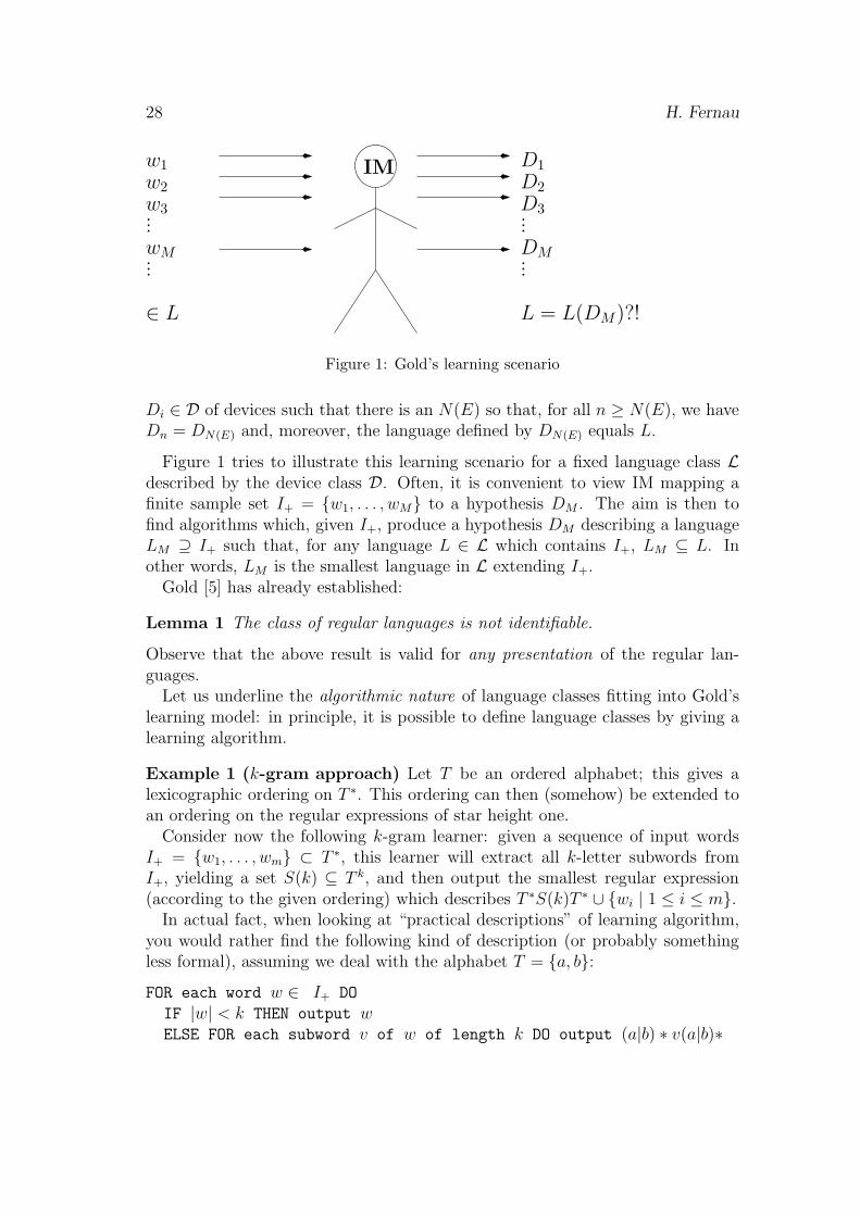
Di ∈ D of devices such that there is an N(E) so that, for all n ≥ N(E), we haveDn = DN(E) and, moreover, the language defined by DN(E) equals L.
Figure 1 tries to illustrate this learning scenario for a fixed language class Ldescribed by the device class D. Often, it is convenient to view IM mapping afinite sample set I+ = {w1, . . . , wM} to a hypothesis DM . The aim is then tofind algorithms which, given I+, produce a hypothesis DM describing a languageLM ⊇ I+ such that, for any language L ∈ L which contains I+, LM ⊆ L. Inother words, LM is the smallest language in L extending I+.
Gold [5] has already established:
Lemma 1 The class of regular languages is not identifiable.
Observe that the above result is valid for any presentation of the regular lan-guages.
Let us underline the algorithmic nature of language classes fitting into Gold’slearning model: in principle, it is possible to define language classes by giving alearning algorithm.
Example 1 (k-gram approach) Let T be an ordered alphabet; this gives alexicographic ordering on T ∗. This ordering can then (somehow) be extended toan ordering on the regular expressions of star height one.
Consider now the following k-gram learner: given a sequence of input wordsI+ = {w1, . . . , wm} ⊂ T ∗, this learner will extract all k-letter subwords fromI+, yielding a set S(k) ⊆ T k, and then output the smallest regular expression(according to the given ordering) which describes T ∗S(k)T ∗ ∪ {wi | 1 ≤ i ≤ m}.
In actual fact, when looking at “practical descriptions” of learning algorithm,you would rather find the following kind of description (or probably somethingless formal), assuming we deal with the alphabet T = {a, b}:FOR each word w ∈ I+ DO
IF |w| < k THEN output wELSE FOR each subword v of w of length k DO output (a|b) ∗ v(a|b)∗
Identifiable Language Classes 29
The interpretation is the the output regular expressions are to be catenated.Observe that the latter description is not independent of the order in which thewords are presented to the learner. Nonetheless, as explained above, it is ratherstraightforward in this case to translate that learning algorithm description intoan algorithm fitting into Gold’s paradigm. Moreover, it is pretty simple to seehere that not all regular languages can be identified, but only (apart from “shortwords”) those which can be desribed as unions of languages of the form T ∗{v}T ∗
for some v ∈ T k.
In general, the (natural) question arises: what language class is actually definedby a given learning algorithm. In actual fact, most of the learning algorithmspublished up to now (and probably even worse: most of the algorithms applied inthe “real world”) are mere heuristics in the sense that nobody ever ventured toexplore what kind of languages can be learnt this way. From a formal languagepoint of view, this gives you a rich source of (small) research topics: just takeany learning heuristic and try to characterize the corresponding language class.Actually, this characterization problem is considered to be one of the most im-portant and challenging tasks both in the area of grammatical inference itself [6]and when you speak with people who build “intelligent” components into largersoftware packages.
2. Function distinguishability
We are now going to define in rather general terms a way to get identifiableregular language classes.
Let F be some finite set. A mapping f : T ∗ → F is called a distinguishingfunction if f(w) = f(z) implies f(wu) = f(zu) for all u, w, z ∈ T ∗. Examplesof distinguishing functions include the terminal function [7] Ter(x) = { a ∈ T |∃u, v ∈ T ∗ : uav = x } and the suffix function Tk(x) yielding the last min(k, |x|)letters of x, corresponding to the k-reversible languages [1]. To every distinguish-ing function f , a finite automaton Af = (F, T, δf , f(λ), F ) can be associated bysetting δf(q, a) = f(wa), where w ∈ f−1(q) can be chosen arbitrarily, since f is adistinguishing function.f -DL can be characterized by f -distinguishable automata defined in the fol-
lowing way:
Definition 2 Let A = (Q, T, δ, q0, QF ) be a finite automaton. Let f : T ∗→F bea distinguishing function. A is called f -distinguishable if:
1. A is deterministic.
2. For all states q ∈ Q and all x, y ∈ T ∗ with δ∗(q0, x) = δ∗(q0, y) = q, we havef(x) = f(y).
(In other words, for q ∈ Q, f(q) := f(x) for some x with δ∗(q0, x) = q iswell-defined.)
30 H. Fernau
3. For all q1, q2 ∈ Q, q1 6= q2, with either (a) q1, q2 ∈ QF or (b) there existq3 ∈ Q and a ∈ T with δ(q1, a) = δ(q2, a) = q3, we have f(q1) 6= f(q2).
There is also a “normal form representation” of languages in L ∈ (-DLf),namely the “stripped version” of Af ×A(L), denoted A(L, f), where A(L) is theminimal state automaton of L.
In [4], we developed an inference algorithm for f -DL based on the state-mergingparadigm, similar to the inference algorithm for 0-reversible languages given byAngluin [1]. As usual, this algorithm starts with the so-called prefix tree au-tomaton obtained from the given input sample I+ from which an automatongenerating I+ plus possibly some other strings has to be induced. More specif-ically, the algorithm keeps merging states as long as there are conflicts in thesestates according to Def. 2. When being implemented by a union-find algorithm,the complexity of the algorithm is basically dependent on the number of unionand of find operations which are triggered by merging of states plus the onestriggered in the initiation phase. More precisely, in the backward nondetermin-ism case, |F | pairs are only created if at least some state of the automaton Af
actually has |F | predecessors. For simplicity, we will call this the indegree of f ,written I(f) for short. In particular, in the automaton ATer, every state has atmost |T | predecessors (where T is the alphabet of the language to be inferred),and the same statement is true for the automaton Aσk
.Our observations can be summarized as follows:
Theorem 2 (Time complexity) By using a standard union-find algorithm, thealgorithm f-Ident as described in [4] can be implemented to run in time
O(α(2(I(f) + 1)(|T | + 1)n, n)(I(f) + 1)(|T | + 1)n),
where α is the inverse Ackermann function and n is the total length of all wordsin I+ from language L, when L is the language presented to the learner for f -DL.
Ignoring the α-term, this means that terminal distinguishable and k-reversiblelanguages can be inferred in time O(|T |2n), which considerably improves thetime bounds from [1, 7]. We currently don’t know how to nicely upperboundI(∆k), where ∆k was defined in [4] in order to generalize the piecewise k-testablelanguages [8].
3. An extended example
Radhakrishnan showed that the language L described by ba∗c + d(aa)∗c lies inTer-DL but its reversal does not. Consider the deterministic (minimal) automa-ton A(L) with transition function δ (see Table 1). Is A(L) Ter-distinguishable?We have still to check whether it is possible to resolve the backward nondeter-minism conflicts (the state 3 occurs two times in the column labelled c). This

Identifiable Language Classes 31
a b c d
→ 0 − 1 − 2
1 1 − 3 −2 4 − 3 −
3 → − − − −4 2 − − −
Ter a b c d
∅ → 0 − 1 − 2
{b} 1 1′ − 3 −{a, b} 1′ 1′ − 3′ −{d} 2 4 − 3′′ −{a, d} 2′ 4 − 3′′′ −{b, c} 3 → − − − −{a, b, c} 3′ → − − − −{c, d} 3′′ → − − − −{a, c, d} 3′′′ → − − − −{a, d} 4 2′ − − −
Ter a b c
∅ → 0 − 1 −{b} 1 1′ − 3
{a, b} 1′ 1′ − 3′
{b, c} 3 → − − −{a, b, c} 3′ → − − −
Table 1: The transition functions δ, δTer and δinferred.
resolution possibility is formalized in the second and third condition in Defini-tion 2. As to the second condition, the question is whether it is possible to assignTer-values to states of A(L) in a well-defined manner: assigning Ter(0) = ∅ andTer(4) = {a, d} is possible, but should we set Ter(1) = {b} (since δ∗(0, b) = 1) orTer(1) = {a, b} (since δ∗(0, ba) = 1)?; similar problems occur with states 2 and 3.Let us therefore try another automaton accepting L, whose transition functionδTer is given by Table 1, we indicate the Ter-values of the states in the first columnof the table. As the reader may verify, δTer basically is the transition table ofthe stripped subautomaton of the product automaton A(L) × ATer. One sourceof backward nondeterminism may arise from multiple final states, see condition3.(a) of Def. 2. Since the Ter-values of all four finite states are different, thissort of nondeterminism can be resolved. Let us consider possible violations ofcondition 3.(b) of Def. 2. In the column labelled a, we find multiple occurrencesof the same state entry:
• δTer(1, a) = δTer(1′, a) = 1′: since Ter(1) = {b} 6= Ter(1′) = {a, b}, this
conflict is resolvable.
• δTer(2, a) = δTer(2′, a) = 4: since Ter(2) = {d} 6= Ter(2′) = {a, d}, this
conflict is resolvable.
Observe that the distinguishing function f can be also used to design efficient“backward scanning” algorithms for languages in f -DL. The only thing one hasto know are the f -values of all prefixes of the word w to be scanned. Let ustry to check that daac belongs to the language L in a backward fashion. Forthe prefixes, we compute: Ter(d) = {d}, Ter(da) = Ter(daa) = {a, d}, andTer(daac) = {a, c, d}. Since Ter(w1) = {a, c, d}, we have to start our backward
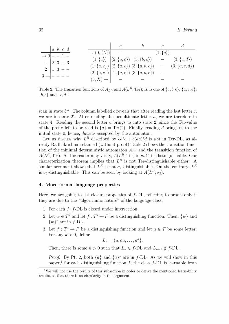
32 H. Fernau
a b c d
→ 0 − − 1 −1 2 3 − 3
2 1 3 − −3 → − − − −
a b c d
→ (0, {λ}) − − (1, {c}) −(1, {c}) (2, {a, c}) (3, {b, c}) − (3, {c, d})
(1, {a, c}) (2, {a, c}) (3, {a, b, c}) − (3, {a, c, d})(2, {a, c}) (1, {a, c}) (3, {a, b, c}) − −(3, X) → − − − −
Table 2: The transition functions of ALR and A(LR,Ter); X is one of {a, b, c}, {a, c, d},{b, c} and {c, d}.
scan in state 3′′′. The column labelled c reveals that after reading the last letter c,we are in state 2′. After reading the penultimate letter a, we are therefore instate 4. Reading the second letter a brings us into state 2, since the Ter-valueof the prefix left to be read is {d} = Ter(2). Finally, reading d brings us to theinitial state 0; hence, daac is accepted by the automaton.
Let us discuss why LR described by ca∗b + c(aa)∗d is not in Ter-DL, as al-ready Radhakrishnan claimed (without proof) Table 2 shows the transition func-tion of the minimal deterministic automaton ALR and the transition function ofA(LR,Ter). As the reader may verify, A(LR,Ter) is not Ter-distinguishable. Ourcharacterization theorem implies that LR is not Ter-distinguishable either. Asimilar argument shows that LR is not σ1-distinguishable. On the contrary, LR
is σ2-distinguishable. This can be seen by looking at A(LR, σ2).
4. More formal language properties
Here, we are going to list closure properties of f -DL, referring to proofs only ifthey are due to the “algorithmic nature” of the language class.
1. For each f , f -DL is closed under intersection.
2. Let w ∈ T ∗ and let f : T ∗→F be a distinguishing function. Then, {w} and{w}∗ are in f -DL.
3. Let f : T ∗ → F be a distinguishing function and let a ∈ T be some letter.For any k > 0, define
Lk = {a, aa, . . . , ak}.Then, there is some n > 0 such that Ln ∈ f -DL and Ln+1 /∈ f -DL.
Proof. By Pt. 2, both {a} and {a}∗ are in f -DL. As we will show in thispaper,1 for each distinguishing function f , the class f -DL is learnable from
1We will not use the results of this subsection in order to derive the mentioned learnabilityresults, so that there is no circularity in the argument.

Identifiable Language Classes 33
text. Due to the result of Gold [5] stating that no superfinite language classis identifiable, we would arrive at a contradiction assuming that the claimof this lemma is not true. 2
4. For any f , f -DL is not closed under union (and hence not under comple-mentation).
Proof. Let f : T ∗ → F be an arbitrary distinguishing function. Considersome a ∈ T . According to Pt. 3, Ln ∈ f -DL and Ln+1 /∈ f -DL for somen > 0. According to Pt. 2, {an+1} ∈ f -DL. If f -DL were closed underunion, then Ln+1 = Ln ∪{an+1} would be in f -DL, too, which is an obviouscontradiction. 2
5. For any f , f -DL is not closed under intersection with finite languages.
Proof. Let f : T ∗ → F be an arbitrary distinguishing function. Considersome a ∈ T . According to Pt. 2, {a}∗ ∈ f -DL. According to Pt. 3, Ln+1 /∈f -DL for some n > 0. If f -DL were closed under intersection with finitelanguages, then Ln+1 = {a}∗ ∩ Ln+1 would belong to f -DL, an obviouscontradiction. 2
Other closure properties cannot be treated in the same uniform way, e.g., thereare distinguishing functions f1 and f2 such that f1-DL is closed under reversals(namely, σk-DL, see [1]) but f2-DL isnot closed under reversals (see Sec. 3).
5. Formal language prospects
Observe one peculiarity in the previous examples (which is typical for languageclasses that can be defined by identification algorithms): it is quite easy to provenon-membership of a certain language into such a class: simply “feed” the lan-guage “in a suitable way” into the learning algorithm and observe overgeneral-ization in one point. In this way, it is often relatively easy to show non-closureproperties which are rather typical for “algorithmically defined” language classes.
Furthermore, note that “on the way”, many well-known (?) formal languagenotions are necessary to actually establish that a certain identification algorithmdescribes a certain language class. Of utmost importance is the “invention” ofsuitable normal forms. This makes it possible that the identification processalways converges to the same automaton (except for state names), irrespectivelyof the order in which the samples are shown to the inference machine.
Using established formal language constructions, function distinguishable lan-guages have been proposed to help infer DTDs for XML documents and in thecase of tree language inference [2, 3].
Finally, identifiable language classes may give rise to new decidability questionsas the suitability of a certain choice of a learnable language class. To be more

34 H. Fernau
concrete, what kind of distinguishing function f should a “user” choose for his/herpurpose? If f is “too simple,” then f -DL might not meet the needs; if f is “toocomplicated,” then the learning process will be rather slow, possibly yieldingintermediate generalizations which are “too complex.”
This gives rise to decidability questions like: Given some regular languagesL1,. . . , Lr, find the “most simple” f such that L1,. . . , Lr are all in f -DL. Thecomplexities of these and similar questions are open (even if r = 1 in the example).
References
[1] D. Angluin. Inference of reversible languages. J. ACM, 29(3):741–765, 1982.
[2] H. Fernau. Learning XML grammars. In Proc. Machine Learning and DataMining in Pattern Recognition MLDM, vol. 2123 of LNCS/LNAI, pp. 73—87,2001.
[3] H. Fernau. Learning tree languages from text. In Computational LearningTheory COLT, vol. 2375 of LNCS/LNAI, pp. 153–168, 2002.
[4] H. Fernau. Identification of function distinguishable languages. Theoret.Comp. Sci., 290:1679–1711, 2003.
[5] E. M. Gold. Language identification in the limit. Inform. & Contr. 10:447–474, 1967.
[6] C. de la Higuera. Current trends in grammatical inference. In Advances inPattern Recognition SSPR+SPR, vol. 1876 of LNCS, pp. 28–31, 2000.
[7] V. Radhakrishnan and G. Nagaraja. Inference of regular grammars via skele-tons. IEEE Trans. Systems, Man and Cybernetics SMC, 17(6):982–992, 1987.
[8] J. Ruiz and P. Garcıa. Learning k-piecewise testable languages from posi-tive data. In Proc. Intern. Coll. Grammatical Inference ICGI, vol. 1147 ofLNCS/LNAI, pp. 203–210, 1996.
P-AUTOMATEN UND ω-P-AUTOMATEN
Rudolf Freund Marion Oswald
Institut fur Computersprachen, Technische Universitat WienFavoritenstraße 9, A-1040 Wien, Osterreich
e-mail: {rudi,marion}@emcc.at
und
Ludwig Staiger
Institut fur Informatik, Martin-Luther-Universitat Halle-WittenbergKurt-Mothes-Straße 1, D-06120 Halle, Germany
e-mail: [email protected]
KURZFASSUNG
Wir untersuchen Varianten von akzeptierenden P-Systemen mit reinen Kommuni-kationsregeln und zeigen, dass diese P-Automaten selbst mit der einfachsten Mem-branstruktur sowohl bei der Akzeptanz von Multimengen als auch bei der Akzeptanzvon Wortern (gegeben als Folge von Terminalsymbolen, die aus der Umgebung ge-holt werden) die gleiche Berechnungskapazitat wie Turingmaschinen besitzen. Beider Akzeptanz von ω-Sprachen erreichen ω-P-Automaten mit zwei Membranen diegleiche Berechnungskapazitat wie ω-Turingmaschinen. Uberdies zeigen wir, dass P-Automaten bzw. ω-P-Automaten, welche aus nur einer Membran bestehen und Re-geln einer sehr eingeschrankten speziellen Form verwenden, regulare Sprachen bzw.ω-regulare Sprachen charakterisieren.
1. Einleitung
Seit der Einfuhrung von Membransystemen durch Gheorghe Paun (s. [12]) imJahre 1998 wurden bereits viele Varianten, welche durch Merkmale biologischerSysteme inspiriert wurden, untersucht. Die Membranstruktur selbst und beson-dere Eigenschaften der Membranen, insbesondere fur den Transport von Ob-jekten, sind die wichtigsten Charakteristika, welche in den verschiedensten Mo-dellen von P-Systemen untersucht werden (s. beispielsweise [2], [14]; fur einenumfassenden Uberblick s. [13], fur den aktuellen Forschungsstand s. [18]). EineMembranstruktur besteht aus Membranen, welche hierarchisch in die außersteMembran (Hautmembran) eingebettet sind; jede Membran umschließt eine Re-gion (Kompartment), welche auch andere Membranen enthalten kann. In dieser
35
36 R. Freund, M. Oswald, L. Staiger
Membranstruktur, wo die Membranen als Separatoren sowie als Kommunikati-onskanale fungieren, konnen sich Objekte entsprechend gegebener Evolutionsre-geln entwickeln. Kurzlich wurden P-Systeme mit reinen Kommunikationsregelneingefuhrt (s. [11]) und weiter untersucht (s. [6], [9]); in diesen P-Systemen mitKommunikationsregeln passieren Objekte die Membranen, ohne selbst von denRegeln verandert zu werden. Passieren Objekte die Membran in derselben Rich-tung, so spricht man von Symport-Regeln, passieren higegen Objekte die Mem-bran in entgegengesetzten Richtungen, so spricht man von Antiport-Regeln.
Die Verwendung von P-Systemen mit Antiport-Regeln als Berechnungs- undErzeugungsmechanismen wurde bereits in [6] untersucht; hier betrachten wir nunwie in [7] derartige P-Systeme als Akzeptierungsmechanismen, die eine (endli-che bzw. unendliche) Eingabe-Folge von Terminalsymbolen analysieren, wie dieszum ersten Mal in [1] betrachtet wurde. Entsprechend der ublichen Notationenin der Theorie formaler Sprachen nennen wir diese Systeme P-Automaten bzw.ω-P-Automaten und zeigen, dass diese die gleiche Berechnungskapazitat wie Tu-ringmaschinen bzw. ω-Turingmaschinen erreichen konnen.
2. Einfuhrende Definitionen und Resultate
Die Menge der nicht-negativen ganzen Zahlen wird mit N0 bezeichnet, die Mengeder positiven ganzen Zahlen mit N. Ein Alphabet V ist eine endliche nicht-leereMenge von abstrakten Symbolen. Das freie Monoid, das von V unter Konka-tenation erzeugt wird, wird mit V ∗ bezeichnet; daruber hinaus definieren wirV + := V ∗ \ {λ} , wobei λ das Leerwort bezeichnet. Eine Multimenge uber Vwird als String uber V (und jede seiner Permutationen) reprasentiert . Mit | x |bezeichnen wir die Lange eines Wortes x uber V sowie die Anzahl der Elementein der Multimenge, die durch x reprasentiert wird. Wir betrachten zwei SprachenL, L′ uber V als gleich, wenn L \ {λ} = L′ \ {λ} .
Ein endlicher Automat (EA) ist ein Quintupel M = (Q, T, δ, q0, F ) , wobei Qeine endliche Menge von Zustanden, T das Eingabealphabet, δ : Q × T → 2Q
die Ubergangsfunktion, q0 ∈ Q den Startzustand und F ⊆ Q die Menge vonEndzustanden bezeichnet. Die Ubergangsfunktion δ kann auf naturliche Weise zueiner Funktion δ : 2Q×T+ → 2Q erweitert werden. Die Sprache, welche von einemEA M akzeptiert wird, ist die Menge aller Worter w ∈ T+ mit δ ({q0} , w)∩F 6= ∅(d.h., aller Worter, welche von M akzeptiert werden). Gilt card (δ (q, a)) = 1 furalle q ∈ Q und alle a ∈ T, so nennt man M einen deterministischen endlichenAutomaten (DEA). Die Familie der von (deterministischen) endlichen Automatenerkannten Mengen stimmt mit der Familie der regularen Mengen uberein.
Betrachten wir Multimengen von Symbolen, so stellen Registermaschinen eineinfaches universelles Berechnungsmodell dar (die ursprunglichen Definitionensind beispielsweise in [10] zu finden, die Definitionen, wie wir sie hier verwenden,in [6] und [8]):
P-Automaten und ω-P-Automaten 37
Eine n-Registermaschine ist ein Konstrukt M = (n,R, i, h) , wobei
• n die Anzahl der Register bezeichnet,
• R eine Menge von markierten Befehlen j : (op (r) , k, l) ist, wobei op (r) eineOperation auf Register r von M ist und j, k, l Markierungen aus der MengeLab (M) sind,
• i die Startmarkierung ist und
• h die Endmarkierung ist.
Die Registermaschine M kennt folgende Befehle:
(A(r),k,l) Addiere eins zum Inhalt des Registers r und fahre mit Befehl k oderBefehl l fort; fur die deterministischen Varianten, welche normalerweise inder Literatur in Betracht gezogen werden, wird k = l gefordert.
(S(r),k,l) Ist Register r nicht leer, dann subtrahiere eins von seinem Inhalt undfahre mit Befehl k fort, sonst fahre mit Befehl l fort.
HALT Halte die Maschine an. Dieser zusatzliche Befehl kann nur der Endmar-kierung h zugeordnet werden.
In der deterministischen Variante konnen solche n-Registermaschinen dazuverwendet werden, partiell rekursive Funktionen f : Nk
0 → Nm0 zu berechnen; be-
ginnend mit (n1, ..., nk) ∈ N0 in den Registern 1 bis k, hat M f (n) = (r1, ..., rm)berechnet, wenn sie in der Endmarkierung h halt und Register 1 bis m r1 bisrm enthalten. Kann die Endmarkierung nicht erreicht werden, so bleibt f (n)undefiniert.
Eine deterministische n-Registermaschine kann auch eine Eingabe (n1, ..., nk) ∈Nk
0 in den Registern 1 bis k analysieren, welche akzeptiert wird, wenn die Re-gistermaschine in der Endmarkierung halt und alle Register leer sind. Halt dieMaschine nicht, so war die Analyse nicht erfolgreich.
In der nicht-deterministischen Variante konnen n-Registermaschinen jede re-kursiv aufzahlbare Menge von naturlichen Zahlen (oder von Vektoren von naturli-chen Zahlen) berechnen. Beginnend mit leeren Registern bezeichnen wir eine Be-rechnung der n-Registermaschine als erfolgreich, wenn sie halt und das Ergebnisin den ersten m Registern enthalten ist (und alle ubrigen Register leer sind).
Aus Ergebnissen in [4] (welche auf wohlbekannten Ergebnissen aus [10] basie-ren) konnen wir Folgendes ableiten:
Proposition 1. Fur jede rekursiv aufzahlbare Menge von Vektoren naturlicherZahlen L ⊆ Nk
0 existiert eine deterministische (k+2)-RegistermaschineM, welcheL erkennt.
Daruber hinaus kennen wir ein ahnliches Ergebnis fur Mengen von Wortern(siehe auch [8]):
38 R. Freund, M. Oswald, L. Staiger
Proposition 2. Fur jede rekursiv aufzahlbare Menge von Wortern L uberdem Alphabet T mit card (T ) = z − 1 existiert eine deterministische 3-Registermaschine M, welche L so erkennt, dass fur jedes w ∈ T ∗ w ∈ L ge-nau dann gilt, wenn M halt, nachdem M mit gz (w) (gz (w) bezeichnet die z-areReprasentation des Wortes w) im ersten Register gestartet wurde.
Bemerkung 3. Auf Grund der Resultate in [10] wissen wir, dass die Aktio-nen einer Turingmaschine durch eine Registermaschine in nur zwei Registernsimuliert werden konnen, indem eine z-are Reprasentation ( z − 1 ist die Kardi-nalitat des Bandalphabets) der linken und rechten Seite des Turingbandes bezogenauf die aktuelle Position des Lese-/Schreibkopfes der Turingmaschine verwendetwird. Dabei verwendet man eine Primzahlkodierung so, dass alle notigen Opera-tionen fur die Simulation der Turingmaschine von einer Registermaschine in nurzwei Registern simuliert werden konnen. Hier benotigen wir nun eine etwas we-niger komprimierte Reprasentation der Aktionen und Inhalte des Arbeitsbandesder Turingmaschine: Wir speichern nur die Inhalte der linken und rechten Seitedes Arbeitsbandes bezogen auf die aktuelle Position des Lese-/Schreibkopfes undsimulieren die Aktionen auf dem Arbeitsband in diesen zwei Registern, wahrendder aktuelle Zustand der Turingmaschine in einem separaten zusatzlichen Regi-ster unar kodiert gespeichert wird.
3. P-Automaten mit Antiport-Regeln
Ein P-Automat mit Antiport-Regeln (fortan einfach P-Automat) ist ein Tupel Πmit
Π = (V, T, µ, w1, ..., wn, R1, ..., Rn, F ) ,
wobei
1. V ein Alphabet von Objekten bezeichnet,
2. T ⊆ V das Terminalalphabet ist,
3. µ eine Membranstruktur ist,
4. w1, ..., wn Multimengen uber V sind, welche mit den Regionen 1, ..., n von µassoziiert sind,
5. R1, ..., Rn endliche Mengen von Antiport-Regeln sind, welche den Membranenbzw. den von ihnen umschlossenen Regionen 1, ..., n zugeordnet und vonder Gestalt (x, out; y, in) mit x, y ∈ V + sind (dabei wird die Multimengex aus der von der Membran umschlossenen Region hinausgeschickt und dieMultimenge y aus der umgebenden Region hereingenommen; der Radius derRegel (x, out; y, in) ist das Zahlenpaar (|x| , |y|)),
6. F eine endliche Menge von Endzustanden ist.
P-Automaten und ω-P-Automaten 39
Ein Endzustand ist eine Funktion f, welche jeder Region eine endliche Mul-timenge zuordnet (s. [1]); ein spezielles Symbol Λ zeigt an, dass der Inhalt derentsprechenden Region nicht in Betracht gezogen werden muss, wahrend fur jedeMultimenge 6= Λ, die einer Membranregion zugeordnet ist, deren Inhalt mit dervorgegebenen endlichen Multimenge ubereinstimmen muss; in diesem Fall sagenwir, dass die zugrundeliegende Konfiguration den Endzustand f erreicht hat. Be-steht die Membranstruktur µ aus nur einer Membran, so kann ein Endzustandeinfach durch die der Hautmembran zugeordnete Multimenge angegeben werden.
Beginnend mit der Startkonfiguration, welche aus µ und w1, ..., wn besteht,erfolgt der Ubergang von einer Konfiguration in die nachste, indem Regeln vonRi nicht-deterministisch und in maximal paralleler Art und Weise angewendetwerden. Eine Berechnung ist eine Folge von Transitionen. Ublicherweise wirdfur eine Multimenge oder ein Wort w uber einem Alphabet T eine Berechnunggenau dann als erfolgreich bezeichnet, wenn sie halt (d.h., wenn keine Regelmehr angewendet werden kann); der Idee der Endzustande folgend wie sie in [1]eingefuhrt wurde, werden wir hier jedoch eine Berechnung dann und nur dannals erfolgreich bezeichnen, wenn ein Endzustand f aus F erreicht wird. EineMultimenge oder ein Wort w uber T wird vom P-Automaten Π dann und nurdann erkannt, wenn es eine erfolgreiche Berechnung von Π so gibt, dass die (Folgevon) Terminalsymbole(n), welche aus der Umgebung genommen wurden, genauw ist. (Falls mehr als ein Terminalsymbol in einem Schritt aus der Umgebunggeholt wird, dann stellt jede Permutation dieser Symbole ein gultiges Teilworteines Eingabewortes dar.)
Das folgende Resultat wurde bereits in [5], allerdings fur haltende P-Automatenund nicht wie hier fur durch Endzustand akzeptierende P-Automaten mitAntiport-Regeln, bewiesen:
Satz 4. Sei L ⊆ Σ∗ eine rekursiv aufzahlbare Sprache. Dann kann L von einemP-Automaten akzeptiert werden, der aus der einfachsten Membranstruktur bestehtund nur Regeln der Form (x, out; y, in) mit Radius (2, 1) oder (1, 2) verwendet.
Beweis. Ausgehend von Proposition 2 zeigen wir, wie wir das Eingabewort w le-sen, die Kodierung gz (w) generieren und dann die Befehle der 3-Registermaschinesimulieren konnen; dabei liegt das Hauptaugenmerk auf der Simulation einer n-Registermaschine:
• Ein Addier-Befehl j : (A (i) , k, l) wird durch die Regeln (j, out; kai, in) und(j, out; lai, in) simuliert.
• Ein bedingter Subtrahier-Befehl j : (S (i) , k, l) wird durch die Regeln(jai, out; k, in) fur den Fall, dass ein Subtraktion moglich ist, sowie an-dernfalls durch die Regeln (j, out; j′j′′, in) , (j′ai, out; #, in) , (j′′, out; ′, in) ,(′, out; ′′, in) , (j′′′, out; l, in) simuliert. Falls das Register i nicht leerist, d.h. mindestens ein Symbol ai vorhanden ist, obwohl man die Regel

40 R. Freund, M. Oswald, L. Staiger
(j, out; j′j′′, in) angewendet hat, dann garantiert die Bedingung der maxima-len Parallelitat , dass im nachsten Schritt die Regel (j′ai, out; #, in) zugleichmit (j′′, out; ′, in) angewendet wird, was zur Einfuhrung des Fehlersym-bols # fuhrt. Nur wenn in der aktuellen Konfiguration kein Symbol ai inder Hautmembran vorkommt, kann das Objekt j′ noch zwei Schritte war-ten, bis es in der Regel (j′′′, out; l, in) zusammen mit dem durch die Regel(′, out; ′′, in) eingefuhrten Symbol ′′ verwendet wird.
• Der Halte-Befehl h : HALT wird dadurch “simuliert”, dass es fur das Hal-tesymbol h keine Regel gibt; da wir davon ausgehen konnen, dass mit Errei-chen des Haltebefehls alle Register der zu simulierenden Registermaschineleer sind, definieren wir daher den Endzustand des zu konstruierenden P-Automaten mit h.
Wir beginnen nun mit q als Axiom und nehmen (q, out; qaa, in) und(qaa, out; qa,0, in) fur jedes a ∈ T. Nehmen wir nun an, die Kodierung der bis zumaktuellen Zeitpunkt eingelesenen Eingabesequenz v werde durch gz (v) SymboleA reprasentiert. Ein weiteres Eingabesymbol a wird durch die Kodierung gz (va)erfasst; wegen gz (va) = z ∗ gz (v) + gz (a) wird dieser Kodierungsschritt durchdas folgende Unterprogramm einer Registermaschine bewerkstelligt, welches imWesentlichen die Multiplikation mit z bewerkstelligt:
qa,0 : (S (1) , qa,1, q′a)
qa,i : (A (2) , qa,i+1, qa,i+1) fur 1 ≤ i < z
qa,z : (A (2) , qa,0, qa,0)
q′a :(
S (2) , q′a,1, q′′a,1
)
q′a,1 : (A (1) , q′a, q′a)
Sei nun k = gz(a); dann horen wir mit den folgenden Befehlen auf:
q′′a,i :(
A (1) , q′′a,i+1, q′′a,i+1
)
fur 1 ≤ i ≤ k − 1
Die Eingabe des nachsten Terminalsymbols beginnt dann mit(
q′′a,ka, out; q, in)
.Offensichtlich konnen die Befehle des obigen Unterprogramms in Antiport-
Regeln ubersetzt werden, wie bereits zu Beginn des Beweises ausgearbeitet wurde.Die Anzahl der Symbole A bzw. B entspricht dem Inhalt von Register 1 bzw. 2.
Wenn kein weiteres Eingabesymbol mehr eingelesen werden soll, verwenden wirdie Antiport-Regeln (q, out; q′q′′, in) , (q′q′′, out; q0, in), um die Simulation der inProposition 2 beschriebenen 3-RegisterMaschine zu starten (dabei entspricht q0der Startmarkierung der Registermaschine).
Offensichtlich erscheint das Haltesymbol h in der Hautmembran dann und nurdann, wenn die Registermaschine die Eingabe gz (w) akzeptiert.
Das Wort, welches erkannt werden soll, ist durch die Folge der Terminalsym-bole a gegeben, welche mittels Antiport-Regeln der Gestalt (q, out; qaa, in) ausder Umgebung geholt wurden. Offensichtlich kann dieses Wort auch als eine Re-prasentation der entsprechenden Multimenge (bzw. des entsprechenden Vektors
P-Automaten und ω-P-Automaten 41
naturlicher Zahlen) interpretiert werden, was zu einem analogen Ergebnis fur re-kursiv aufzahlbare Multimengen uber T (bzw. fur die entsprechenden Mengenvon Vektoren naturlicher Zahlen) fuhrt.
3.1. Endliche P-Automaten mit Antiport-Regeln
Wenn wir P-Automaten betrachten, die aus der einfachsten Membranstruktur,d.h. nur der Hautmembran, bestehen, und nur Regeln sehr spezieller Form ver-wenden, erhalten wir eine Charakterisierung der Familie der regularen Sprachen,was im Folgenden gezeigt wird:
Ein endlicher P-Automat ist ein P-Automat
Π = (V, T, [1]1, w1, R1, F )
mit nur einer Membran, wobei
1. das Axiom w1 ein Nichtterminal ist, d.h., w1 ∈ V \ T (im Fall endlicher P-Automaten bezeichnen wir ein Element aus V \T einfach auch als Zustand);
2. die Antiport-Regeln in R1 von der Gestalt (q, out; pa, in) und (pa, out; r, in)mit a ∈ T und p, q, r ∈ V \ T sind;
3. fur jede Regel (q, out; pa, in) in R1 die einzigen anderen Regeln in R1, welchep enthalten, von der Gestalt (pa, out; r, in) sind;
4. F ⊆ V \ T (jede Multimenge in F besteht aus genau einem Zustand).
Satz 5. Sei L ⊆ Σ+. Dann ist L genau dann regular, wenn L von einemendlichen P-Automaten akzeptiert wird.Beweis. Sei L eine regulare Sprache, welche von einem EA M = (Q, T, δ, q0, F )akzeptiert wird. Dann wird L auch von dem endlichen P-Automaten Π =(V, T, [1]1, q0, R1, F ) akzeptiert, wobei
V = Q ∪ {(q, a, r) | r ∈ δ (q, a) fur q, r ∈ Q, a ∈ T} ∪ T und
R1 = {(p, out; (q, a, r)a, in) , ((q, a, r) a, out; r, in) | p, q, r ∈ Q, a ∈ T und r ∈ δ (q, a)} .Jeder Ubergang (q, a, r) in M wird in Π durch die Regeln (p, out; (q, a, r) a, in)
und ((q, a, r)a, out; r, in) in zwei Schritten simuliert. Dabei enthalt die Hautmem-bran in der intermediaren Konfiguration (q, a, r) a.
Auf der anderen Seite kann nun eine regulare Sprache L, die von einem endli-chen P-Automaten Π = (V, T, [1]1, q0, R1, F ) erkannt wird, auch von einem endli-chen Automaten M = (V \ T, T, δ, q0, F ) akzeptiert werden, wobei
δ = {((q, a) , {r ∈ V \ T | (q, out; pa, in) , (pa, out; r, in) ∈ R1 fur p ∈V \ T}) |q ∈ V \ T, a ∈ T} .
Jede Anwendung einer Folge (q, out; pa, in) , (pa, out; r, in) von Regeln aus R1
wird durch nur einen Ubergang (q, a, r) in M simuliert; da die intermediarenInhalte pa der Hautmembran nicht als Endzustand fungieren konnen, muss ineiner erfolgreichen Berechnung von M die Anwendung einer Regel (q, out; pa, in)

42 R. Freund, M. Oswald, L. Staiger
von der Anwendung von (pa, out; r, in) fur ein r ∈ V \ T gefolgt werden, womitdie Transitionen in δ die Regeln in R1 korrekt simulieren.
4. ω-Turingmaschinen
Wir betrachten den Raum Xω der unendlichen Worter (ω-Worter) auf einemendlichen Alphabet X mit card (X) ≥ 2. Sei w · b die Konkatenation von w ∈ X∗
und b ∈ Xω, welche sich auf naturliche Weise auf Teilmengen W ⊆ X∗ undB ⊆ Xω erweitern laßt. Teilmengen von Xω werden ω-Sprachen genannt. Fur einω-Wort ξ und jedes n ∈ N bezeichnet ξ/n den Prafix von ξ der Lange n.
In den meisten Modellen, die in der Literatur gefunden werden (s. beispielswei-se [3] oder [17]), wird die Akzeptanz von ω-Sprachen durch Turingmaschinen vomVerhalten auf dem Eingabeband sowie durch spezifische Endzustandsbedingun-gen, die von der Akzeptanz von ω-Sprachen durch endliche Automaten bekanntsind, determiniert.
Entsprechend den X-Automaten von Engelfriet und Hoogeboom (s. [3]) be-trachten wir ω-Turingmaschinen als Automaten M = (X,Γ, Q, q0, P ) mit einemseparaten Eingabeband, auf welchem sich der Lesekopf nur nach rechts bewegenkann, einem Arbeitsband, einem Eingabealphabet X, dem Bandalphabet Γ, einerendlichen Menge interner Zustande Q, dem Anfangszustand q0 und der Relation
P ⊆ Q×X × Γ ×Q× {0,+1} × Γ × {−1, 0,+1} ,welche die nachste Konfiguration definiert.
Wenn sich M im Zustand q ∈ Q befindet sowie x0 ∈ X auf dem Eingabebandund x1 ∈ Γ auf dem Arbeitsband liest, so bedeutet (q, x0, x1; p, y0, y1, y2) ∈ P,dass M in den Zustand p ∈ Q ubergeht, den Kopf auf dem Eingabeband nachrechts bewegt, wenn y0 = +1 oder den Kopf nicht bewegt, wenn y0 = 0, und fury1 ∈ Γ und y2 ∈ {−1, 0,+1} die Maschine y1 an Stelle von x1 auf das Arbeitsbandschreibt und den Kopf auf dem Band nach links bewegt, wenn y2 = −1, nachrechts, wenn y2 = +1, oder gar nicht bewegt, wenn y2 = 0.
Sei ξ ∈ Xω die Eingabe der ω-Turingmaschine M. Wir nennen eine Folge z ∈Qω von Zustanden einen Lauf vonM auf ξ, wenn die Folge von Zustanden, welchedie Turingmaschine in ihrer Berechnung mit Eingabe ξ durchlauft, z ist. Wirsagen, dass eine Eingabefolge ξ ∈ Xω vonM gemaß Bedingung C akzeptiert wird,wenn es einen derartigen Lauf z von M auf ξ gibt, dass z Bedingung C erfullt.In Anlehnung an die Notationen von Engelfriet und Hoogeboom betrachten wirfolgende Bedingungen: Sei α : Qω → 2Q eine Abbildung, die jedem ω-Wort ζ ∈ Qω
eine Teilmenge Q′ ⊆ Q zuordnet, und sei R ⊆ 2Q × 2Q eine Relation zwischenTeilmengen von Q. Wir sagen, dass ein Paar (M,Y ) fur Y ⊆ 2Q ein ω-Wortξ ∈ Xω genau dann akzeptiert, wenn
∃Q′∃z (Q′ ∈ Y ∧ z ist ein Lauf von M auf ξ ∧ (α (z) , Q′) ∈ R) .
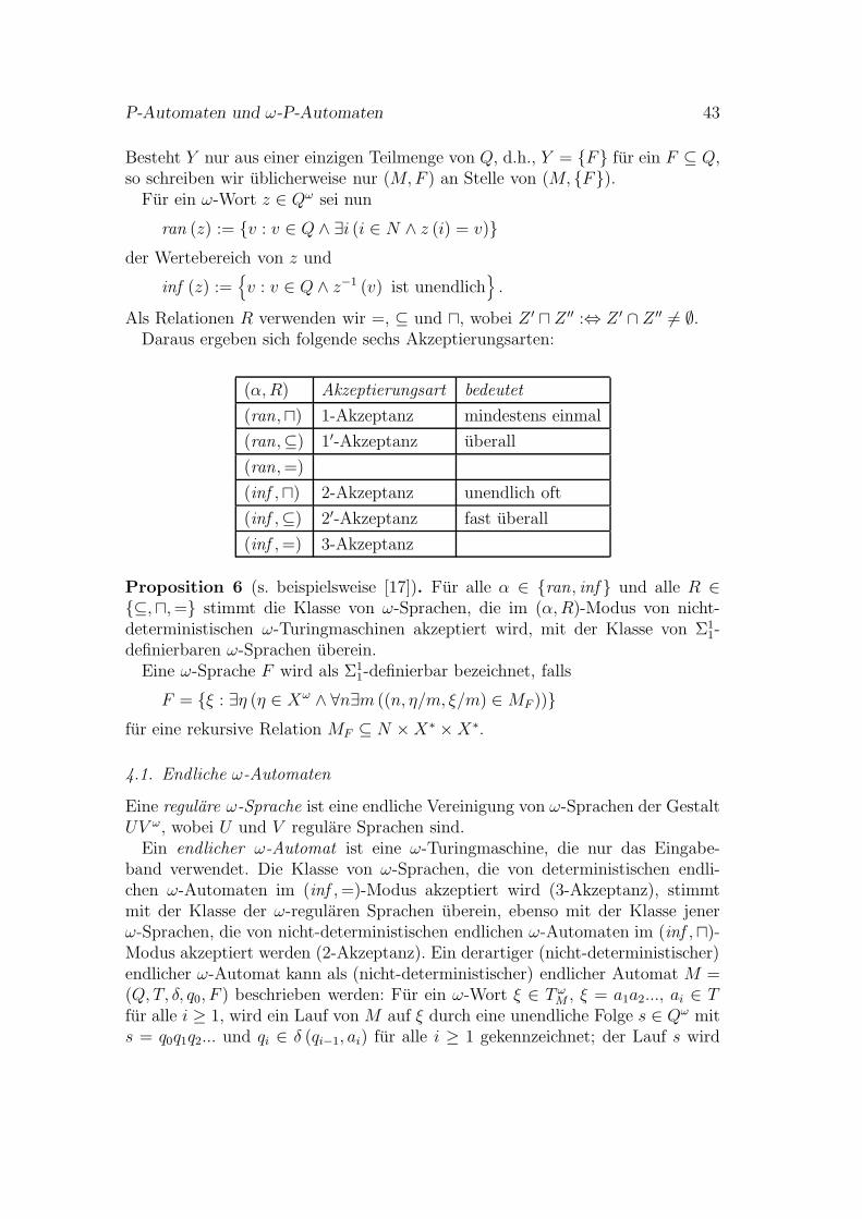
P-Automaten und ω-P-Automaten 43
Besteht Y nur aus einer einzigen Teilmenge von Q, d.h., Y = {F} fur ein F ⊆ Q,so schreiben wir ublicherweise nur (M,F ) an Stelle von (M, {F}).
Fur ein ω-Wort z ∈ Qω sei nun
ran (z) := {v : v ∈ Q ∧ ∃i (i ∈ N ∧ z (i) = v)}der Wertebereich von z und
inf (z) :={
v : v ∈ Q ∧ z−1 (v) ist unendlich}
.
Als Relationen R verwenden wir =, ⊆ und ⊓, wobei Z ′ ⊓ Z ′′ :⇔ Z ′ ∩ Z ′′ 6= ∅.Daraus ergeben sich folgende sechs Akzeptierungsarten:
(α,R) Akzeptierungsart bedeutet
(ran,⊓) 1-Akzeptanz mindestens einmal
(ran,⊆) 1′-Akzeptanz uberall
(ran,=)
(inf ,⊓) 2-Akzeptanz unendlich oft
(inf ,⊆) 2′-Akzeptanz fast uberall
(inf ,=) 3-Akzeptanz
Proposition 6 (s. beispielsweise [17]). Fur alle α ∈ {ran, inf } und alle R ∈{⊆,⊓,=} stimmt die Klasse von ω-Sprachen, die im (α,R)-Modus von nicht-deterministischen ω-Turingmaschinen akzeptiert wird, mit der Klasse von Σ1
1-definierbaren ω-Sprachen uberein.
Eine ω-Sprache F wird als Σ11-definierbar bezeichnet, falls
F = {ξ : ∃η (η ∈ Xω ∧ ∀n∃m ((n, η/m, ξ/m) ∈ MF ))}fur eine rekursive Relation MF ⊆ N ×X∗ ×X∗.
4.1. Endliche ω-Automaten
Eine regulare ω-Sprache ist eine endliche Vereinigung von ω-Sprachen der GestaltUV ω, wobei U und V regulare Sprachen sind.
Ein endlicher ω-Automat ist eine ω-Turingmaschine, die nur das Eingabe-band verwendet. Die Klasse von ω-Sprachen, die von deterministischen endli-chen ω-Automaten im (inf ,=)-Modus akzeptiert wird (3-Akzeptanz), stimmtmit der Klasse der ω-regularen Sprachen uberein, ebenso mit der Klasse jenerω-Sprachen, die von nicht-deterministischen endlichen ω-Automaten im (inf ,⊓)-Modus akzeptiert werden (2-Akzeptanz). Ein derartiger (nicht-deterministischer)endlicher ω-Automat kann als (nicht-deterministischer) endlicher Automat M =(Q, T, δ, q0, F ) beschrieben werden: Fur ein ω-Wort ξ ∈ T ω
M , ξ = a1a2..., ai ∈ Tfur alle i ≥ 1, wird ein Lauf von M auf ξ durch eine unendliche Folge s ∈ Qω mits = q0q1q2... und qi ∈ δ (qi−1, ai) fur alle i ≥ 1 gekennzeichnet; der Lauf s wird

44 R. Freund, M. Oswald, L. Staiger
im Sinne der 2-Akzeptanz als erfolgreich bezeichnet, wenn inf (s) ∩ F 6= ∅. Dievon M akzeptierte ω-Sprache ist die Menge aller ξ ∈ T ω, die einen erfolgreichenLauf von M auf ξ erlauben.
5. ω-P-Automaten mit Antiport-Regeln
Im Fall von ω-Wortern mussen wir nicht nur die (jetzt unendliche) Folge vonTerminalsymbolen, die von der Umgebung geholt werden, beachten, sondern auchdie Akzeptanzbedingung, welche uber die Endzustande definiert ist.
Ein ω-P-Automat ist ein Konstrukt
Π = (V, T, µ, w1, ..., wn, R1, ..., Rn, Y ) ,
das wie ein P-Automat definiert ist, allerdings jetzt zur Analyse unendlicherFolgen von Terminalsymbolen und deren Akzeptanz in Ubereinstimmung mitder gegebenen Akzeptanzbedingung zusammen mit einer Menge Y, Y ⊆ 2Q,verwendet wird. Jede Menge F ∈ Y stellt eine endliche Menge von Endzustndendar.
Der Beweis des folgenden Hauptergebnisses basiert auf den Beobachtungen inBemerkung 3:
Satz 7. Sei L ⊆ Σωeine ω-Sprache, die von einer ω-Turingmaschine im Akzep-tanzmodus (α,R) , α ∈ {ran , inf } , R ∈ {⊆,⊓,=} , akzeptiert wird. Dann konnenwir einen ω-P-Automaten mit zwei Membranen konstruieren, der die Aktioneneiner Turingmaschine simuliert, L im selben Akzeptanzmodus (α,R) akzeptiertund nur Regeln der Gestalt (x, out; y, in) mit Radius (2, 1) bzw. (1, 2) , verwendet.
Beweis. Sei L ⊆ Σω eine ω-Sprache, die von einer ω-Turingmaschine
M = (Σ,Γ, Q, q0, P )
zusammen mit Y ⊆ 2Q im Akzeptanzmodus (α,R) akzeptiert wird.Wir konstruieren nun einen ω-P-Automaten
Π = (V,Σ, [1[2]2]1, q′0, fg, R1, R2, Y
′)
mit zwei Membranen und Antiport-Regeln der Form (x, out; y, in) mit Radius(2, 1) bzw. (1, 2), der die Aktionen der Turingmaschine simuliert und L im selbenAkzeptanzmodus (α,R) akzeptiert. Dabei simulieren wir eine RegistermaschineRM mit nur drei Registern, welche ihrerseits wiederum die Aktionen von M da-durch simuliert, dass eine z-are Reprasentation der linken und rechten Seite desTuringbandes in zwei Registern simuliert wird (wobei z − 1 die Kardinalitat desBandalphabetes ist) und der aktuelle Zustand von M in einem separaten zusatz-lichen Register unar kodiert gespeichert wird. Die komplexeren Schritte von Mkonnen von Π in mehreren Unterschritten simuliert werden:
Das Einlesen eines neuen Symbols b ∈ Σ auf dem Eingabeband von M kanndurch Regeln (q, out; (q, b, r) b, in) und ((q, b, r) b, out; r, in) , q, r ∈ V \ T, im ω–P-Automaten Π simuliert werden. Das Andern der linken und rechten Seite des
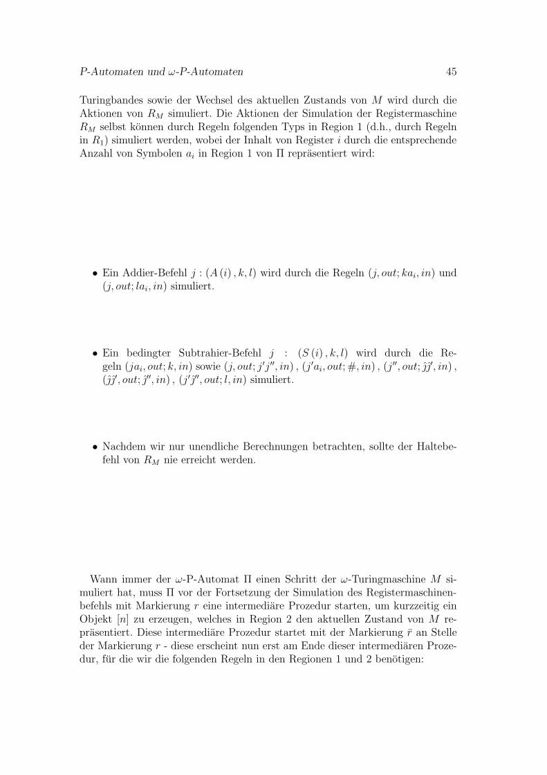
P-Automaten und ω-P-Automaten 45
Turingbandes sowie der Wechsel des aktuellen Zustands von M wird durch dieAktionen von RM simuliert. Die Aktionen der Simulation der RegistermaschineRM selbst konnen durch Regeln folgenden Typs in Region 1 (d.h., durch Regelnin R1) simuliert werden, wobei der Inhalt von Register i durch die entsprechendeAnzahl von Symbolen ai in Region 1 von Π reprasentiert wird:
• Ein Addier-Befehl j : (A (i) , k, l) wird durch die Regeln (j, out; kai, in) und(j, out; lai, in) simuliert.
• Ein bedingter Subtrahier-Befehl j : (S (i) , k, l) wird durch die Re-geln (jai, out; k, in) sowie (j, out; j′j′′, in) , (j′ai, out; #, in) , (j′′, out; ′, in) ,(′, out; ′′, in) , (j′′′, out; l, in) simuliert.
• Nachdem wir nur unendliche Berechnungen betrachten, sollte der Haltebe-fehl von RM nie erreicht werden.
Wann immer der ω-P-Automat Π einen Schritt der ω-Turingmaschine M si-muliert hat, muss Π vor der Fortsetzung der Simulation des Registermaschinen-befehls mit Markierung r eine intermediare Prozedur starten, um kurzzeitig einObjekt [n] zu erzeugen, welches in Region 2 den aktuellen Zustand von M re-prasentiert. Diese intermediare Prozedur startet mit der Markierung r an Stelleder Markierung r - diese erscheint nun erst am Ende dieser intermediaren Proze-dur, fur die wir die folgenden Regeln in den Regionen 1 und 2 benotigen:
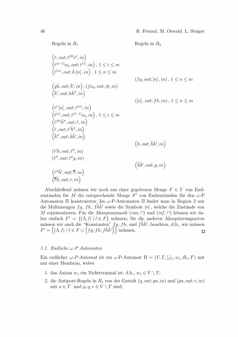
46 R. Freund, M. Oswald, L. Staiger
Regeln in R1 Regeln in R2
(
r, out; r(0)r′, in)
(
r(i−1)a3, out; r(i), in
)
, 1 ≤ i ≤ m(
r(n), out; h [n] , in)
, 1 ≤ n ≤ m
(fg, out; [n] , in) , 1 ≤ n ≤ m(
gh, out; h′, in)
, (fa3, out; #, in)(
h′, out; hh′′, in)
([n] , out; fh, in) , 1 ≤ n ≤ m(
r′ [n] , out; r(n), in)
(
r(i), out; r(i−1)a3, in)
, 1 ≤ i ≤ m(
r(0)h′′, out; r, in)
(
r, out; r′h′′, in)
(
h′′, out; hh′, in)
(
h, out; hh′, in)
(r′h, out; r′′, in)
(r′′, out; r′′g, in)(
hh′, out; g, in)
(
r′′h′, out; r, in)
(
rh, out; r, in)
Abschließend mussen wir noch aus einer gegebenen Menge F ∈ Y von End-zustanden fur M die entsprechende Menge F ′ von Endzustanden fur den ω-PAutomaten Π konstruieren: Im ω-P-Automaten Π findet man in Region 2 nurdie Multimengen fg, fh, f hh′ sowie die Symbole [n] , welche die Zustande vonM reprasentieren. Fur die Akzeptanzmodi (ran,⊓) und (inf ,⊓) konnen wir da-her einfach F ′ = {(Λ, l) | l ∈ F} nehmen; fur die anderen Akzeptierungsartenmussen wir auch die “Konstanten” fg, fh, und fhh′, beachten, d.h., wir mussenF ′ =
{
(Λ, l) | l ∈ F ∪{
fg, fh, f hh′}}
nehmen.
5.1. Endliche ω-P Automaten
Ein endlicher ω-P-Automat ist ein ω-P-Automat Π = (V, T, [1]1, w1, R1, F ) mitnur einer Membran, wobei
1. das Axiom w1 ein Nichtterminal ist, d.h., w1 ∈ V \ T ;
2. die Antiport-Regeln in R1 von der Gestalt (q, out; pa, in) und (pa, out; r, in)mit a ∈ T und p, q, r ∈ V \ T sind;
P-Automaten und ω-P-Automaten 47
3. fur jede Regel (q, out; pa, in) in R1 die einzigen anderen Regeln in R1, welchep enthalten, von der Gestalt (pa, out; r, in) sind;
4. F ⊆ V \ T .
Satz 8. Sei L ⊆ Σω eine ω-Sprache. Dann ist L genau dann ω-regular, wenn Lvon einem endlichen ω-P-Automaten im 2-Akzeptanzmodus akzeptiert wird.Beweis. Wir verwenden die gleiche Konstruktion wie in Satz 5; interpretieren wirnun den dort betrachteten endlichen Automaten als endlichen ω-Automaten undden dort konstruierten endlichen P-Automaten als endlichen ω-P-Automaten, soerhalten wir sofort das gewunschte Ergebnis.
Literatur
[1] Csuhaj-Varju, E., Vaszil, G.: P automata. In: [15], 177–192
[2] Dassow, J., Paun, Gh.: On the power of membrane compu-ting. Journal of Universal Computer Science 5, 2 (1999) 33–49(http://www.iicm.edu/jucs)
[3] Engelfriet, J., Hoogeboom, H.J.: X-automata on ω-words. Theoret. Comput.Sci. 110,1 (1993) 1–51
[4] Freund, R., Oswald, M.: Generalized P systems with forbidding context.Fundamenta Informaticae 49, 1-3 (2002) 81–102
[5] Freund, R., Oswald, M.: A short note on analysing P systems with antiportrules. Bulletin EATCS, 78 (2002) 231–236
[6] Freund, R., Oswald, M.: P systems with activated/prohibited membranechannels. In: Paun, Gh., Rozenberg, G., Salomaa, A., Zandron, C. (Eds.):Membrane Computing 2002. Lecture Notes in Computer Science, Springer,Berlin (2002)
[7] Freund, R., Oswald, M., Staiger, L.: ω-P automata with communication ru-les. In: Alhazov, A., Martın-Vide, C., Paun, Gh. (Eds.): Proceedings of Work-shop on Membrane Computing (WMC-2003), Tarragona (2003) 252–265
[8] Freund, R., Paun, Gh.: On the number of non-terminals in graph-controlled,programmed, and matrix grammars. In: Margenstern, M., Rogozhin, Y.(Eds.): Proc. Conf. Universal Machines and Computations, Chisinau (2001)
[9] Frisco, P., Hoogeboom, H. J.: Simulating counter automata by P systemswith symport/antiport. In [15], 237–248
[10] Minsky, M. L.: Finite and Infinite Machines. Prentice Hall, Englewood Cliffs,New Jersey (1967)
[11] Paun, A., Paun, Gh.: The power of communication: P systems with sym-port/antiport. New Generation Computing 20, 3 (2002) 295–306
48 R. Freund, M. Oswald, L. Staiger
[12] Paun, Gh.: Computing with membranes. Journal of Computer and SystemSciences 61, 1 (2000) 108–143
[13] Paun, Gh.: Membrane Computing - An Introduction. Springer-Verlag, Berlin(2002)
[14] Paun, Gh., Rozenberg, G., Salomaa, A.: Membrane computing with exter-nal output. Fundamenta Informaticae 41 (3) (2000) 259–266, and TUCSResearch Report No. 218, 1998 (http://www.tucs.fi)
[15] Paun, Gh., Zandron, C. (Eds.): Pre-Proceedings of Workshop on MembraneComputing (WMC-CdeA2002), Curtea de Arges, Romania (2002)
[16] Rozenberg, G., Salomaa, A. (Eds.): Handbook of Formal Languages.Springer-Verlag, Berlin (1997)
[17] Staiger, L.: ω-languages. In: [16], Vol. 3, 339–387
[18] The P Systems Web Page: http://psystems.disco.unimib.it

UBER MEHRDIMENSIONALEREBOUND-AUTOMATEN
Jens Glockler
Institut fur InformatikUniversitat Giessen
Arndtstr. 2, D-35392 Giessene-mail: [email protected]
KURZFASSUNG
Wir betrachten mehrdimensionale Rebound-Automaten und vergleichen sie mitMehrkopfautomaten sowie Automaten mit beschrankten Zahlern. Die dichte Hierar-chie fur Mehrkopfautomaten (bzgl. der Anzahl der Lesekopfe) impliziert eine eben-solche Hierarchie fur die Dimension der Rebound-Automaten. Weiterhin betrachtenwir die Moglichkeit, auf das Abprallen des Lesekopfes an einigen der
”Wande“ seines
Eingabebandes zu verzichten.
Rebound-Automaten wurden 1977 von Morita, Sugata und Umeo eingefuhrt(s. [3, 4]) und z.B. in [1, 5, 6, 7, 8] aufgegriffen. Ein (zweidimensionaler) Re-bound-Automat ist ein endlicher Automat, der sich (nur lesend) auf einem qua-dratischen Band bewegt, welches in der ersten Zeile das zu verarbeitende Einga-bewort enthalt und sonst mit Leerfeldern beschriftet ist:
0 1 2 3 4 5 6 7 80
1
2
3
4
5
6
7
8
b b b ba a a a
Ein k-dimensionaler Rebound-Automat besitzt entsprechend ein Eingabeband inder Form eines k-dimensionalen Hyperwurfels, das an einer
”Kante“ mit dem
(eindimensionalen) Eingabewort beschriftet ist.
48
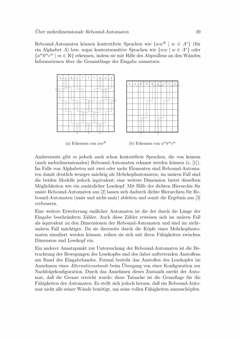
Uber mehrdimensionale Rebound-Automaten 49
Rebound-Automaten konnen kontextfreie Sprachen wie {wwR | w ∈ A∗} (furein Alphabet A) bzw. sogar kontextsensitive Sprachen wie {ww | w ∈ A∗} oder{ambmcm | m ∈ N} erkennen, indem sie mit Hilfe des Abprallens an den WandenInformationen uber die Gesamtlange der Eingabe ausnutzen:
0 1 2 3 4 5 6 7 8 9 100
1
2
3
4
5
6
7
8
9
10
a c b a b b a b c a
(a) Erkennen von wwR
0 1 2 3 4 5 6 7 8 90
1
2
3
4
5
6
7
8
9
a a a b b b c c c
(b) Erkennen von ambmcm
Andererseits gibt es jedoch auch schon kontextfreie Sprachen, die von keinem(auch mehrdimensionalen) Rebound-Automaten erkannt werden konnen (s. [1]).Im Falle von Alphabeten mit zwei oder mehr Elementen sind Rebound-Automa-ten damit deutlich weniger machtig als Mehrkopfautomaten, im unaren Fall sinddie beiden Modelle jedoch aquivalent; eine weitere Dimension bietet dieselbenMoglichkeiten wie ein zusatzlicher Lesekopf. Mit Hilfe der dichten Hierarchie furunare Rebound-Automaten aus [2] lassen sich dadurch dichte Hierarchien fur Re-bound-Automaten (unar und nicht-unar) ableiten und somit die Ergebnis aus [3]verbessern.
Eine weitere Erweiterung endlicher Automaten ist die der durch die Lange derEingabe beschrankten Zahler. Auch diese Zahler erweisen sich im unaren Fallals aquivalent zu den Dimensionen der Rebound-Automaten und sind im nicht-unaren Fall machtiger. Da sie ihrerseits durch die Kopfe eines Mehrkopfauto-maten simuliert werden konnen, reihen sie sich mit ihren Fahigkeiten zwischenDimension und Lesekopf ein.
Ein anderer Ansatzpunkt zur Untersuchung der Rebound-Automaten ist die Be-trachtung der Bewegungen des Lesekopfes und des dabei auftretenden Anstoßensam Rand des Eingabebandes. Formal besteht das Anstoßen des Lesekopfes imAnnehmen eines Alternativzustands beim Ubergang von einer Konfiguration zurNachfolgekonfiguration. Durch das Annehmen dieses Zustands merkt der Auto-mat, daß die Grenze erreicht wurde; diese Tatsache ist die Grundlage fur dieFahigkeiten des Automaten. Es stellt sich jedoch heraus, daß ein Rebound-Auto-mat nicht alle seiner Wande benotigt, um seine vollen Fahigkeiten auszuschopfen.

50 J. Glockler
Im zweidimensionalen Fall kann auf die Beruhrung einer der vier Wande verzich-tet werden, bei Hinzunahme weiterer Dimensionen kann fur jede Dimension dienicht an die Eingabe grenzende Wand ausgespart werden.
Literatur
[1] Inoue, K., Takanami, I. und Taniguchi, H. A note on rebound auto-mata. Information Sciences 26 (1982), 87–93.
[2] Monien, B. Two-way multihead automata over a one-letter alphabet. RAI-RO – Theoretical Informatics and Applications 14 (1980), 67–82.
[3] Morita, K., Sugata, K. und Umeo, H. Computation complexity ofn-bounded counter automaton and multidimensional rebound automaton.Systems, Computers, Controls 8 (1977), 80–87. Ubersetzung von [4].
[4] Morita, K., Sugata, K. und Umeo, H. Computation complexity ofn-bounded counter automaton and multidimensional rebound automaton.Denshi Tsushin Gakkai Ronbunshi 60-D (1977), 283–290.
[5] Petersen, H. Fooling rebound automata. In Proc. MFCS 1999 (1999),Band 1672 der LNCS, Springer-Verlag, S. 241–250.
[6] Petersen, H. Separation results for rebound automata. In Proc. MFCS2000 (2000), Band 1893 der LNCS, Springer-Verlag, S. 589–598.
[7] Sakamoto, M., Inoue, K. und Takanami, I. A two-way nondetermi-nistic one-counter language not accepted by nondeterministic rebound auto-mata. The Transactions of the IEICE E 73 (1990), 879–881.
[8] Sugata, K., Umeo, H. und Morita, K. The language accepted by arebound automaton and its computing ability. Electronics and Communica-tions in Japan 60-A (1977), 11–18.
A COMMON ALGEBRAIC CHARACTERIZATION OFPROBABILISTIC AND QUANTUM COMPUTATIONS
Martin Beadury
Departement de mathematiques et d’informatiqueUniversite de Sherbrooke, 2500, boul. Universite
Sherbrooke (Quebec), J1K 2R1 Canadae-mail: [email protected]
Jose M. Fernandez
Departement d’I.R.O., Universite de MontrealC.P. 6128 succ. Centre-Ville
Montreal, (Quebec), H3C 3J7 Canadae-mail: [email protected]
and
Markus Holzer
Institut fur Informatik, Technische Universitat MunchenBoltzmannstraße 3, D-85748 Garching bei Munchen, Germany
e-mail: [email protected]
ABSTRACT
Through the study of gate arrays we develop a unified framework to deal withprobabilistic and quantum computations, where the former is shown to be a naturalspecial case of the latter. On this basis we define show how to encode a probabilisticor quantum gate array into a sum-free tensor formula which satisfies the conditionsof the partial trace problem, and vice-versa. This allows us to define a meaningfulcomputational problem on tensor formula, called the partial trace tensor formulaproblem, which is fundamental to our studies, which allows us to capture importantcomplexity classes like, PP, pr-BPP (promise BPP), pr-BQP (promise BQP), andmany others, as the underlying algebraic structure varies.
Keywords: Quantum computing, probabilistic computing, tensor algebra, complex-ity theory.
The “algebraic” approach in the theory of computational complexity consistsin characterizing complexity classes within unified frameworks built around acomputational model or problem involving an algebraic structure (usually finite
51
52 M. Beaudry, J. M. Fernandez, M. Holzer
or finitely generated) as the main parameter. In this way, various complexityclasses are seen to share the same definition, up to the choice of the underlyingalgebra. Successful examples of this approach include the description of NC1 andits subclasses AC0 and ACC0 in terms of polynomial-size programs over finitemonoids [1], and analogous results for PSPACE, the polynomial hierarchy andthe polytime mod-counting classes, through the use of polytime leaf languages [5].A more recent example is the complexity of problems whose input is a tensor for-mula, i.e., a fully parenthesized expression where the inputs are matrices (givenin full) over some finitely generated algebra and the allowed operations are ma-trix addition, multiplication, and tensor product, also known as outer, or direct,or Kronecker product. Evaluating tensor formulas with explicit tensor entries isshown by Damm et. al [3] to be complete for ⊕P, for NP, and for #P as thesemiring varies. Recently also other common sense computational problems ontensor formulas and tensor circuits were analyzed by Beaudry and Holzer [2].Tensor formulas are a compact way of specifying very large matrices. As such,they immediately find a potential application in the description of the behaviorof circuits, be they classical Boolean, arithmetic (tensor formulas over the appro-priate semiring) or quantum (formulas over the complex field, or an adequatelychosen sub-semiring thereof).
We formalize and confirm this intuition, that basic tensor calculus not onlycaptures natural complexity classes in simple ways, but it yields a simpler andunified view on classical probabilistic and modern quantum computation, whichgives probabilistic and quantum computations the exact same definition, up tothe underlying algebra. Apart from offering a first application of the algebraicapproach to quantum computing, our paper thus reasserts the point made byFortnow [4], that for the classes BPP and BQP, the jump from classical to quan-tum polynomial-time computation consists in allowing negative matrix entries forthe evolution operators, which means that different computations done in parallelmay interfere destructively. Based on this unified framework, we define a mean-ingful computational problem on tensor formula, called the partial trace tensorformula problem, which is fundamental to our studies, which allows us to captureimportant complexity classes; that is given a tensor formula F of order n×1 overa semiring S plus a positive integer k, deciding whether the kth partial trace ofthe matrix valn,n
S (F ·FT) fulfills a certain property. Our precise characterizationsare as follows:
• We present probabilistic computation as a natural special case of quantumcomputation using the unified framework on gate arrays, instead of present-ing quantum as a more or less artificial extension of probabilistic computa-tion.
• The partial trace sum-free tensor formula problem enables us to capturethe significant complexity classes (pr-)P (promise P), NP, pr-BPP (promiseBPP), and PP and some of their quantum counterparts pr-EQP (promise
A common characterization of probabilistic and quantum computations 53
EQP), NQP, and pr-BQP (promise BQP), by showing completeness resultsof the problem under consideration.
• By giving up sum-freeness, we obtain completeness statements for furthercomplexity classes like ⊕P, NP, C=P, its complement co-C=P, Valiant’sclass pr-UP (promise UP), its generalization pr-SPP (promise SPP), andunique polytime US.
Since some of these classes are “semantic” classes, i.e., the underlying machinemust obey a property for all inputs, which is not obvious to check, or evenundecidable. An example would be UP, since for a nondeterministic machineto define a language in UP, it must have the property that for all inputs eitherexactly one accepting path exists or none. Therefore, the obtained completenessresults are subject to a certain promise.
References
[1] D. Mix Barrington and D. Therien. Finite monoids and the fine structure ofNC1. Journal of the ACM, 35(4):941–952, October 1988.
[2] M. Beaudry and M. Holzer. The complexity of tensor circuit evaluation. InJ. Sgall, A. Pultr, and P. Kolman, editors, Proceedings of the 26th Conferenceon Mathematical Foundations of Computer Science, number 2136 in LNCS,pages 173–185, Marianske Lazne, Czech Republic, August 2001. Springer.
[3] C. Damm, M. Holzer, and P. McKenzie. The complexity of tensor calculus.Computational Complexity, 2003. Accepted for publication.
[4] L. Fortnow. One complexity theorist’s view of quantum computing. Theoret-ical Computer Science, 292(3):597–610, 2003.
[5] U. Hertrampf, C. Lautemann, T. Schwentick, H. Vollmer, and K. W. Wag-ner. On the power of polynomial time bit-reductions. In Proceedings of the8th Annual Structure in Complexity Theory Conference, pages 200–207, SanDiego, California, May 1993. IEEE Computer Society Press.

DISTANCE AUTOMATA AND THE STAR HEIGHT
PROBLEM
Daniel Kirsten1
LIAFAUniversite Denis Diderot – Case 7014
2, place JussieuF-75251 Paris Cedex 05, France
e-mail: [email protected]
ABSTRACT
Distance automata were introduced by K. Hashiguchi motivated by his re-search on the star height hierarchy in 1982 [2, 3]. Distance automata became afruitful concept in theoretical computer science with many applications beyondtheir impact for the decidability of the star height hierarchy [4], e.g., they havebeen of crucial importance in the research on the star problem in trace monoids[6, 10], but they are also of interest in industrial applications as speech process-ing [11]. Consequently, distance automata and related concepts have been studiedby many researchers beside K. Hashiguchi, e.g., [5, 7, 8, 9, 12, 13].
Let Σ be a finite alphabet. A distance automaton is a tuple A = [Q,E, I, F,∆],where
1. [Q,E, I, F ] is an automaton (i.e., Q is a finite set, E ⊆ Q × Σ × Q, andI, F ⊆ Q are initial resp. accepting states) and
2. ∆ : E → {0, 1} is a mapping called distance function.
Let A = [Q,E, I, F,∆] be a distance automaton. We extend ∆ to paths: wedefine the distance of a path π as the sum of the distances of all transitions in πand denote it by ∆(π). We define the distance of a word w ∈ Σ∗ as the minimumover the distances of all successful paths which are labeled with w. Under theconvention min ∅ = ∞, A computes a mapping ∆ : Σ∗ → N ∪∞.
We define L(A) as the language all words w ∈ Σ∗ for which ∆(w) 6= ∞. Thisis exactly the language of the automaton [Q,E, I, F ].
54
Distance automata and the star height problem 55
Distance automata are more involved than classic automata, e.g., there arenondeterministic distance automata which do not admit a deterministic equiv-alent, and it is undecidable whether two distance automata compute the samemapping [7].
A distance automaton is limited if there is a bound d ∈ N such that ∆(w) ≤d for every w ∈ L(A). The limitedness problem for distance automata is thequestion for an algorithm which decides whether a distance automaton is limitedor not. It was already raised by C. Choffrut in the framework of recognizablepower series over the tropical semiring in 1979 [1].
In 1982, K. Hashiguchi showed that the limitedness problem for distanceautomata is decidable. In 1987, H. Leung showed that it is PSPACE-hard [8],and very recently, H. Leung and V. Podolskiy showed that it is PSPACE-complete [9].
In the talk we introduce desert automata by associating another semantics todistance automata. Formally, desert automata are defined exactly as distanceautomata. Let A = [Q,E, I, F,∆] be a desert automaton. We call a transitione ∈ E a water transition if ∆(e) = 1.
Let π and π′ paths in A. We call π′ a subpath of π if there are (possibly empty)paths π1 and π2 in A such that π1π
′π2 = π.Imagine that you plan to walk through a desert for a few weeks. You carry a
water tank which is initially full but it not last the entire way. However, you visitseveral places during your journey where you can find some water and refill thetank. Clearly, the required capacity of the tank is determined by the maximaldistance between two consecutive water places. If you have the choice betweenseveral paths, then you intend to carry a rather small but sufficient tank, andthus, you choose a path for which the required capacity of the tank is minimal.
Thus, we define the distance of a path π as the length of a longest subpathof π which does not contain any water transition, and denote it by ∆′(π). Wedefine for every word w ∈ Σ∗ ∆′(w) as the minimum of the values ∆′(π) for allsuccessful paths π which are labeled by w.
A desert automaton is limited if there is a bound d ∈ N such that ∆′(w) ≤ dfor every w ∈ L(A). The limitedness problem for desert automata is the questionfor an algorithm which decides whether a desert automaton is limited or not.
We explain by an example that the limitedness problem for desert automatacannot be decided by a trivial pumping argument.
We define a suitable notion of transformation matrices of desert automata, andwe reduce the limitedness problem for desert automata to a Burnside type prob-lem for the semigroup of transformation matrices. We solve this Burnside typeproblem by applying results from finite semigroup theory and developing tech-niques from I. Simon’s and H. Leung’s approaches to the limitedness problemfor distance automata.
Hence, we can show that the limitedness problem for desert automata is de-cidable in time and space complexity 2O(n2) where n is the number of states.

56 D. Kirsten
Moreover, we show that this problem is PSPACE-hard.Finally, we will discuss some further developments and important consequences
for the star height problem.
References
[1] C. Choffrut. Series rationelles d’image finie. Technical Report 79–6, Labo-ratoire d’Informatique Theorique et Programmation, Paris, 1979.
[2] K. Hashiguchi. Limitedness theorem on finite automata with distance func-tions. Journal of Computer and System Sciences, 24:233–244, 1982.
[3] K. Hashiguchi. Regular languages of star heigth one. Information and Con-trol, 53:199–210, 1982.
[4] K. Hashiguchi. Algorithms for determining relative star heigth and starheigth. Information and Computation, 78:124–169, 1988.
[5] K. Hashiguchi. New upper bounds to the limitedness of distance automata.Theoretical Computer Science, 233:19–32, 2000.
[6] D. Kirsten and J. Marcinkowski. Two techniques in the area of the starproblem in trace monoids. Theoretical Computer Science, to appear in 2003.
[7] D. Krob. The equality problem for rational series with multiplicities inthe tropical semiring is undecidable. International Journal of Algebra andComputation, 4(3):405–425, 1994.
[8] H. Leung. An Algebraic Method for Solving Decision Problems in FiniteAutomata Theory. PhD thesis, Pennsylvania State University, Departmentof Computer Science, 1987.
[9] H. Leung and V. Podolskiy. The limitedness problem on distance automata:Hashiguchi’s method revisited. Theoretical Computer Science, to appear in2003.
[10] Y. Metivier and G. Richomme. New results on the star problem in tracemonoids. Information and Computation, 119(2):240–251, 1995.
[11] M. Mohri. Finite-state transducers in language and speech processing. Com-putational Linguistics, 23:269–311, 1997.
[12] I. Simon. On semigroups of matrices over the tropical semiring. InformatiqueTheorique et Applications, 28:277–294, 1994.
[13] A. Weber. Distance automata having large finite distance or finite ambiguity.Mathematical Systems Theory, 26:169–185, 1993.

ON THE NP-COMPLETENESS OF THE Nurikabe
PUZZLE AND VARIANTS THEREOF
Markus Holzer
Institut fur Informatik, Technische Universitat Munchen,Boltzmannstraße 3, D-85748 Garching bei Munchen, Germany
e-mail: [email protected]
Andreas Klein
Fachbereich fur Mathematik und Informatik, Universitat Kassel,Heinrich Plett Straße 40, D-34132 Kassel, Germany
e-mail: [email protected]
and
Martin Kutrib
Institut fur Informatik, Universitat Gießen,Arndtstraße 2, D-35392 Gießen, Germany
e-mail: [email protected]
ABSTRACT
We show that the popular pencil puzzle Nurikabe is intractible from the compu-tational complexity point of view, i.e., is NP-complete. To this end we show howto simulate Boolean gates by the puzzle under consideration. Moreover, we studysome variant of Nurikabe, which remains NP-complete, too.
Keywords: Pencil puzzle game, complexity theory, intractability, completeness.
Nurikabe (engl. coating wall) is a solitaire puzzle, which was invented byNikoli & Time Intermedia, a Japenese publisher. The puzzle takes place ona finite rectangular two-dimensional grid, with some cells or blocks filled withnatural numbers. The goal is to fill the blocks according to the following rules:
1. You cannot fill in blocks containing numbers.
2. A number defines the number of continuous white blocks—they are linkedeither horizontal or vertical. Each area of white blocks contains only onenumber in it and they are separated by black blocks. Digonal connectionsdo not count.
57
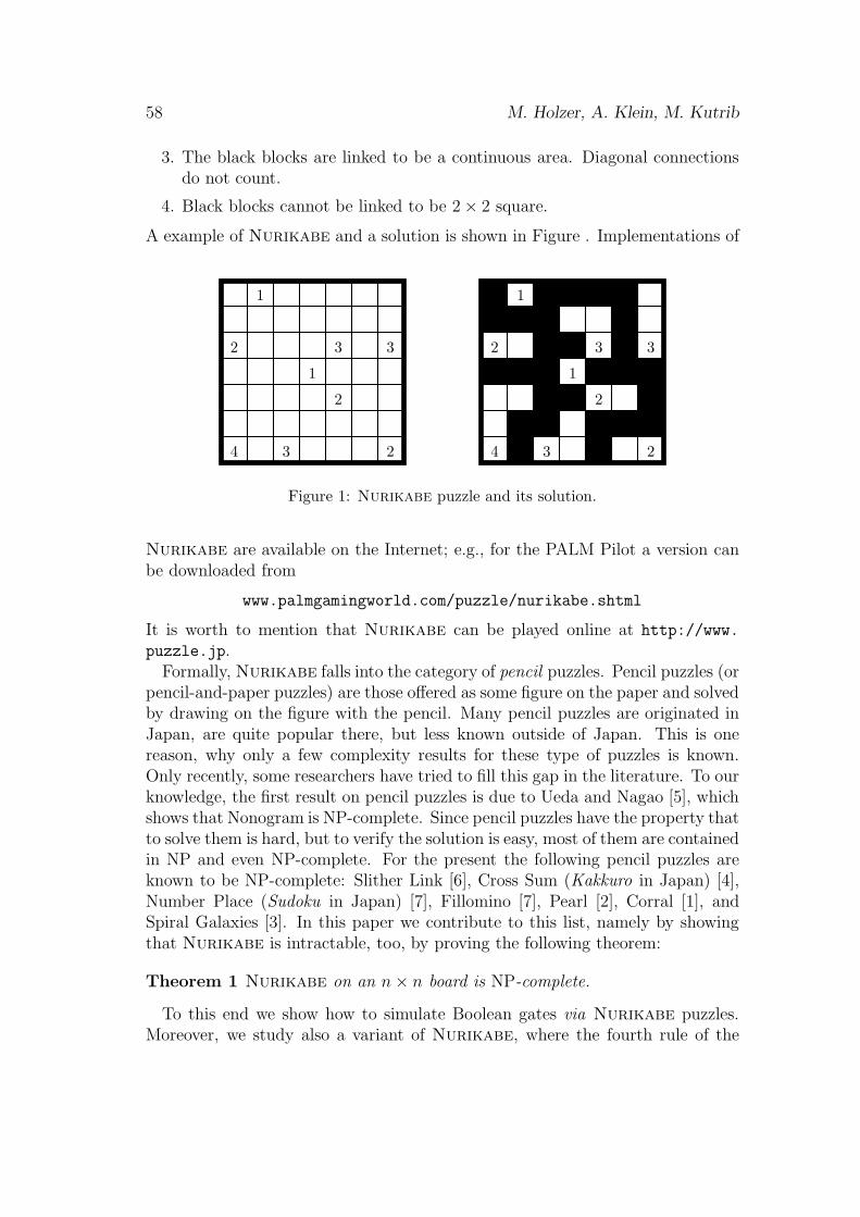
58 M. Holzer, A. Klein, M. Kutrib
3. The black blocks are linked to be a continuous area. Diagonal connectionsdo not count.
4. Black blocks cannot be linked to be 2 × 2 square.
A example of Nurikabe and a solution is shown in Figure . Implementations of
1
2
4
1
2
23
3 3
1
2
4
1
2
23
3 3
Figure 1: Nurikabe puzzle and its solution.
Nurikabe are available on the Internet; e.g., for the PALM Pilot a version canbe downloaded from
www.palmgamingworld.com/puzzle/nurikabe.shtml
It is worth to mention that Nurikabe can be played online at http://www.
puzzle.jp.Formally, Nurikabe falls into the category of pencil puzzles. Pencil puzzles (or
pencil-and-paper puzzles) are those offered as some figure on the paper and solvedby drawing on the figure with the pencil. Many pencil puzzles are originated inJapan, are quite popular there, but less known outside of Japan. This is onereason, why only a few complexity results for these type of puzzles is known.Only recently, some researchers have tried to fill this gap in the literature. To ourknowledge, the first result on pencil puzzles is due to Ueda and Nagao [5], whichshows that Nonogram is NP-complete. Since pencil puzzles have the property thatto solve them is hard, but to verify the solution is easy, most of them are containedin NP and even NP-complete. For the present the following pencil puzzles areknown to be NP-complete: Slither Link [6], Cross Sum (Kakkuro in Japan) [4],Number Place (Sudoku in Japan) [7], Fillomino [7], Pearl [2], Corral [1], andSpiral Galaxies [3]. In this paper we contribute to this list, namely by showingthat Nurikabe is intractable, too, by proving the following theorem:
Theorem 1 Nurikabe on an n× n board is NP-complete.
To this end we show how to simulate Boolean gates via Nurikabe puzzles.Moreover, we study also a variant of Nurikabe, where the fourth rule of the
On the NP-completeness of the Nurikabe puzzle and variants thereof 59
game description is not present. In this case, it is shown, that the pencil puzzlegame remains intractable, namely NP-complete.
References
[1] E. Friedman. Corral puzzles are NP-complete. Technical report, Stet-son University, DeLand, FL 32723, 2002. www.stetson.edu/ efried-man/papers/corral.ps.
[2] E. Friedman. Pearl puzzles are NP-complete. Technical report, Stet-son University, DeLand, FL 32723, 2002. www.stetson.edu/ efried-man/papers/pearl.ps.
[3] E. Friedman. Spiral galaxies puzzles are NP-complete. Technical report,Stetson University, DeLand, FL 32723, 2002. www.stetson.edu/ efried-man/papers/spiral.ps.
[4] T. Seta. The complexities of CROSS SUM. IPSJ SIG Notes, AL-84:51–58,2002. (in Japanese).
[5] N. Ueda and T. Nagao. NP-completeness results for NONOGRAM via parsi-monious reductions. Technical Report TR96-0008, Department of ComputerScience, Tokyo Institute of Technology, 1996.
[6] T. Yato. On the NP-completness of the slither link puzzle. IPSJ SIG Notes,AL-74:25–32, 2000. (in Japanese).
[7] T. Yato. Complexity and completeness of finiding another solution and itsapplication to puzzles. Master thesis, Graduate School of Science, Universityof Tokyo, January 2003.
EINE KOMBINATORISCHE EIGENSCHAFTGEWISSER 0, 1-MATRIZENRoman KönigUniversität Erlangen-Nürnberg, Institut für Informatik IIIMartensstraÿe 3, 91058 Erlangen, Germanye-mail: koenig�informatik.uni-erlangen.deKURZFASSUNG1. EinleitungDie Datenanalyse befasst si h mit der Aufgabe, in grossen Datenbeständen Regel-mäÿigkeiten zu entde ken. Datenbestände stellt man si h dabei zunä hst so vor,dass man eine Relation zwis hen einer Menge G von Gegenständen (=Transaktio-nen, in der Spra he der Datenbanktheorie) und einer Menge M von Merkmalen(=Attributen) gegeben hat. Je na h Anwendung kann man si h diese Relation alsein 0, 1−Matrix oder eine Tabelle mit Kreuzen an den Stellen (g,m) ∈ G×M , fürdie die Aussage: �Der Gegenstand g besitzt das Merkmal m� zutri�t, vorstellen.Sol he Tabellen heiÿen Kontexte, die Relation wird gewöhnli h mit I bezei h-net. Bei der Betra htung von redundanzfreien Kontexten zur Bes hreibung allerendli hen Hüllensysteme treten die folgenden Matrizen auf.2. Die Matrizen An und CnDie Matrizen An und Cn sind 2n−reihige 0, 1−Matrizen mit der De�nitionC0 = × , A0 =
Cn+1 =Cn An
Cn × und An+1 =An ×An An
(n ≥ 0) (2.1)wobei das Symbol× die Matrix passender Gröÿe bezei hnet, die an allen Stellenden Eintrag 1 besitzt. In der De�nition von An+1 und Cn+1 hat also × die60
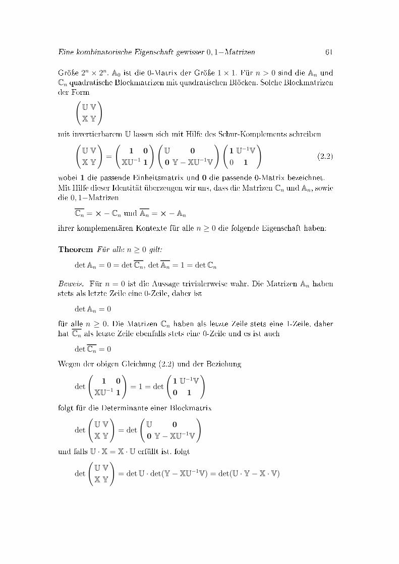
Eine kombinatoris he Eigens haft gewisser 0, 1−Matrizen 61Gröÿe 2n × 2n. A0 ist die 0-Matrix der Gröÿe 1 × 1. Für n > 0 sind die An undCn quadratis he Blo kmatrizen mit quadratis hen Blö ken. Sol he Blo kmatrizender Form
(
U V
X Y
)mit invertierbarem U lassen si h mit Hilfe des S hur-Komplements s hreiben(
U V
X Y
)
=
(
1 0
XU−1 1
)(
U 0
0 Y − XU−1V
)(
1 U−1V
0 1
) (2.2)wobei 1 die passende Einheitsmatrix und 0 die passende 0-Matrix bezei hnet.Mit Hilfe dieser Identität überzeugen wir uns, dass die Matrizen Cn und An, sowiedie 0, 1−MatrizenCn = × − Cn und An = × − Anihrer komplementären Kontexte für alle n ≥ 0 die folgende Eigens haft haben:Theorem Für alle n ≥ 0 gilt:det An = 0 = det Cn, det An = 1 = det CnBeweis. Für n = 0 ist die Aussage trivialerweise wahr. Die Matrizen An habenstets als letzte Zeile eine 0-Zeile, daher istdet An = 0für alle n ≥ 0. Die Matrizen Cn haben als letzte Zeile stets eine 1-Zeile, daherhat Cn als letzte Zeile ebenfalls stets eine 0-Zeile und es ist au hdet Cn = 0Wegen der obigen Glei hung (2.2) und der Beziehungdet
(
1 0
XU−1 1
)
= 1 = det
(
1 U−1V
0 1
)folgt für die Determinante einer Blo kmatrixdet
(
U V
X Y
)
= det
(
U 0
0 Y − XU−1V
)und falls U · X = X · U erfüllt ist, folgtdet
(
U V
X Y
)
= det U · det(Y − XU−1V) = det(U · Y − X · V)
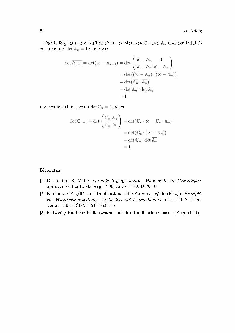
62 R. KönigDamit folgt aus dem Aufbau (2.1) der Matrizen Cn und An und der Indukti-onsannahme det An = 1 zunä hst:det An+1 = det(× − An+1) = det
(
× − An 0
× − An × − An
)
= det(
(× − An) · (× − An))
= det(An · An)
= det An · det An
= 1und s hlieÿli h ist, wenn det Cn = 1, au hdet Cn+1 = det
(
Cn An
Cn ×
)
= det(Cn · × − Cn · An)
= det(Cn · (× − An))
= det Cn · det An
= 1Literatur[1℄ B. Ganter, R. Wille: Formale Begri�sanalyse: Mathematis he Grundlagen.Springer Verlag Heidelberg, 1996, ISBN 3-540-60868-0[2℄ B. Ganter: Begri�e und Implikationen, in: Stumme, Wille (Hrsg.): Begri�i- he Wissensverarbeitung � Methoden und Anwendungen, pp.1 - 24, SpringerVerlag, 2000, ISBN 3-540-66391-6[3℄ R. König: Endli he Hüllensystem und ihre Implikationenbasen (eingerei ht)
ON THE DESCRIPTIONAL POWER OF HEADS,
COUNTERS, AND PEBBLES
Martin Kutrib
Institut fur Informatik, Universitat GiessenArndtstr. 2, D-35392 Giessen, Germany
e-mail: [email protected]
ABSTRACT
We investigate the descriptional complexity of deterministic two-way k-head finiteautomata (k-DHA). It is shown that between deterministic finite automata (DFA)and any k-DHA, k ≥ 2, there are savings in the size of description which can-not be bounded by any recursive function. The same is true for the other end ofthe hierarchy. Such non-recursive trade-offs are also shown between any k-DHA andDSPACE(log) = multi-DHA. We also address the particular case of unary languages.In general, it is possible that non-recursive trade-offs for arbitrary languages reduceto recursive trade-offs for unary languages. Here we present enormous lower boundsfor the unary trade-offs between DFA and any k-DHA, k ≥ 2. Furthermore, severalknown simulation results imply the presented trade-offs for other descriptional sys-tems, e.g. deterministic two-way finite automata with k pebbles or with k linearlybounded counters.
Keywords: Descriptional complexity, non-recursive trade-offs, k-head finite au-tomata.
Formal languages can have many representations in the world of automata,grammars and other rewriting systems, language equations, logical formulas etc.So it is natural to investigate the succinctness of their representation by differentmodels in order to optimize the space requirements. The regular languages areone of the first and most intensely studied language families. It is well knownthat nondeterministic finite automata (NFA) can offer exponential savings inspace compared with deterministic finite automata (DFA). Concerning the num-ber of states, 2n is a tight bound for the NFA to DFA conversion [8]. For example,asymptotically bounds are O(nn) for the two-way DFA to one-way DFA conver-sion [8], 2O(n2) for the two-way NFA to one-way DFA conversion [9], O(
√2n) for
the two-way DFA to one-way NFA conversion [1], and O(2n+3) for the two-wayNFA to one-way NFA conversion [1]. The latter reference is a valuable source forfurther simulation results.
63
64 M. Kutrib
All mentioned trade-offs in the number of states are bounded by recursive func-tions. But, for example, there is no recursive function which bounds the savingsin descriptional complexity between deterministic and unambiguous pushdownautomata [12]. In [10] it is proved that the trade-off between unambiguous andnondeterministic pushdown automata is also non-recursive. Recent results in-volving the parallel model of cellular automata can be found in [5]. In particular,non-recursive trade-offs are shown there between DFA and real-time one-waycellular automata (real-time OCA), between pushdown automata and real-timeOCA, and between real-time OCA and real-time two-way cellular automata.
A comprehensive survey of descriptional complexity of machines with limitedresources is [3] which is a valuable source for further results and references.
Nevertheless, some challenging problems of finite automata are open. An im-portant example is the question how many states are sufficient and necessary tosimulate two-way NFA with two-way DFA. The problem has been raised in [9]and partially solved in [11].
When certain problems are difficult to resolve in general, a natural questionconcerns simpler versions. To this regard promising research has been done forunary languages. It turned out that this particular case is essentially differentfrom the general case. The problem of evaluating the costs of unary automatasimulations has been raised in [11]. In [2] it has been shown that the unary NFA
to DFA conversion takes eΘ(√
n·ln(n)) states, the NFA to two-way DFA conversionhas been solved with a bound of O(n2) states, and the costs of the unary two-
way to one-way DFA conversion reduces to eΘ(√
n·ln(n)). Several more resultscan be found in [6, 7]. Furthermore, in [5] it is shown for real-time OCA thatnon-recursive trade-offs for arbitrary languages reduce to recursive trade-offs forunary languages.
Here we investigate the descriptional complexity of deterministic two-way k-head finite automata (k-DHA). In particular, we consider the trade-offs betweenDFA and k-DHA for any k ≥ 2, and the trade-offs between any k-DHA and thedeterministic log-space bounded Turing machines whose languages are exactlythe languages accepted by the union of all k-DHA. All these trade-offs are shownto be non-recursive. For unary languages it is not known whether the trade-offsare recursive or not. Here we present enormous lower bounds between DFA andany k-DHA. Furthermore, these lower bounds increase with the number of headsin a nice way. Provided minimality can be shown, these bounds can also serve aslower bounds between k-DHA and (k + 1)-DHA.
The results are adapted to other types of acceptors, e.g. deterministic two-way finite automata with k pebbles or with k linearly bounded counters. Someconcerned and related open questions are discussed.
On the descriptional power of heads, counters, and pebbles 65
References
[1] Birget, J.-C. State-complexity of finite-state devices, state compressibility andincompressibility . Math. Systems Theory 26 (1993), 237–269.
[2] Chrobak, M. Finite automata and unary languages. Theoret. Comput. Sci. 47(1986), 149–158.
[3] Goldstine, J., Kappes, M., Kintala, C. M. R., Leung, H., Malcher, A., andWotschke, D. Descriptional complexity of machines with limited resources. J.UCS 8 (2002), 193–234.
[4] Hartmanis, J. On the succinctness of different representations of languages. Inter-national Colloquium on Automata, Languages and Programming (ICALP 1979),LNCS 71, 1979, pp. 282–288.
[5] Malcher, A. Descriptional complexity of cellular automata and decidability ques-tions. J. Autom. Lang. Comb. 7 (2002), 549–560.
[6] Mereghetti, C. and Pighizzini, G. Two-way automata simulations and unary lan-guages. J. Autom. Lang. Comb. 5 (2000), 287–300.
[7] Mereghetti, C. and Pighizzini, G. Optimal simulations between unary automata.SIAM J. Comput. 30 (2001), 1976–1992.
[8] Meyer, A. R. and Fischer, M. J. Economy of description by automata, grammars,and formal systems. IEEE Symposium on Switching and Automata Theory, 1971,pp. 188–191.
[9] Sakoda, W. J. and Sipser, M. Nondeterminism and the size of two way finite au-tomata. ACM Symposium on Theory of Computing (STOC 1978), 1978, pp. 275–286.
[10] Schmidt, E. M. and Szymanski, T. G. Succinctness of descriptions of unambiguouscontext-free languages. SIAM J. Comput. 6 (1977), 547–553.
[11] Sipser, M. Lower bounds on the size of sweeping automata. J. Comput. SystemSci. 21 (1980), 195–202.
[12] Valiant, L. G. A note on the succinctness of descriptions of deterministic lan-guages. Inform. Control 32 (1976), 139–145.

VERIFICATION OF NON-REGULAR PROPERTIES
Martin Lange
Institut fur InformatikLudwig-Maximilians-Universitat Munchen
e-mail: [email protected]
ABSTRACT
We present a game-based formalism that can be used to do local model checkingfor FLC, a modal fixed point logic that extends the µ-calculus with a sequentialcomposition operator. This logic is capable of expressing non-regular propertieswhich are interesting for verification purposes.
1. Introduction
The modal µ-calculus [2] is an important specification language for the verificationof temporal properties. This is mainly due to the fact that it subsumes mosttemporal, dynamic or description logics.
On the other hand, the modal µ-calculus is equi-expressive to Monadic SecondOrder Logic [1], i.e. it can only describe “regular” properties. In [7], Muller-Olmhas introduced FLC, Fixed Point Logic with Chop, which extends the modal µ-calculus with a sequential composition operator, and has shown that its expressivepower is not limited by regularity. In fact, it is not hard to define the language{anbncn | n ∈ N} in FLC on words for example.
On finite structures, FLC’s model checking problem is decidable [7]. In [5], atableau formalism was introduced that can be used to do global model checking.Here we present a game-based framework [4] for local model checking. Thesegames cannot deny a certain similarity with alternating push-down automataover trees. Just as FLC extends the modal µ-calculus, they extend its modelchecking games [8].
We also give examples of FLC-definable properties that are interesting forverification purposes and present the most important results on FLC.
66

Verification of non-regular properties 67
2. Preliminaries
A transition system T = (S, { a→ | a ∈ A}, L) over a set P = {tt, ff, q, q, . . .}of propositional constants consists of states, transition relations and a labellingfunction from states to sets of propositions. Formulas of FLC are given by
ϕ ::= q | Z | τ | 〈a〉 | [a] | ϕ ∨ ϕ | ϕ ∧ ϕ | µZ.ϕ | νZ.ϕ | ϕ;ϕ
where q ∈ P, a ∈ A, and Z ∈ V, a set of propositional variables. We will write σfor µ or ν. Formulas are assumed to be well named in the sense that each bindervariable is distinct. Our main interest is with closed formulas, that do not havefree variables, in which case there is a function fp : V → FLC that maps eachvariable to its defining fixed point formula. The set Sub(ϕ) of subformulas of ϕand its alternation depth ad(ϕ) are defined as usual.The tail of a variable Z in a formula ϕ, tlZ is a set consisting of those formulasthat occur “behind” Z in fp(Z) in ϕ. We use sequential composition for sets offormulas in a straightforward way: {ϕ0, . . . , ϕn};ψ := {ϕ0;ψ, . . . , ϕn;ψ}. Let
tlZ(ψ) := {ψ} if ψ ∈ P ∪ {τ, 〈a〉, [a] | a ∈ A} tlZ(σY.ψ) := tlZ(ψ)
tlZ(ϕ ∨ ψ) = tlZ(ϕ ∧ ψ) := tlZ(ϕ) ∪ tlZ(ψ) tlZ(Y ) :=
{
{Y } if Y 6= Z
{τ} o.w.
tlZ(ϕ;ψ) :=
{
tlZ(ϕ);ψ if Z ∈ Sub(ϕ)
{τ} o.w.
}
∪{
tlZ(ψ) if Z ∈ Sub(ψ)
{τ} o.w.
}
The tail of Z in ϕ is simply calculated as tlZ := tlZ(fp(Z)).An important factor in the complexity of FLC’s model checking problem is the
sequential depth sd(ϕ) of a formula. Informally the sequential depth of a formulais the maximal number of times a variable is sequentially composed with itself.It is defined as sd(ϕ) := max{sdZ(fp(Z)) | Z ∈ Sub(ϕ)} − 1 where
sdZ(ϕ ∨ ψ) := max{sdZ(ϕ), sdZ(ψ)} sdZ(ϕ ∧ ψ) := max{sdZ(ϕ), sdZ(ψ)}sdZ(ϕ;ψ) := sdZ(ϕ) + sdZ(ψ) sdZ(σY.ϕ) := sdZ(ϕ)
sdZ(ψ) := 0 if ψ ∈ {q, τ, 〈a〉, [a]} sdZ(Y ) :=
{
1 if Y = Z
0 o.w.
To simplify the notation of a formula’s semantics we assume a transition systemT to be fixed for the remainder of the paper. In order to handle open formulaswe need environments ρ : V → (2S → 2S). ρ[Z 7→ f ] is the function that maps Zto f and agrees with ρ on all other arguments.
The semantics [[·]]Tρ : 2S → 2S of an FLC formula, relative to T and ρ, is amonotone function on subsets of states with respect to the inclusion ordering on2S . These functions together with the partial order given by
f ⊑ g iff ∀X ⊆ S : f(X) ⊆ g(X)
68 M. Lange
form a complete lattice with joins ⊔ and meets ⊓. By the Tarski-Knaster Theorem[9] the least and greatest fixed points of functionals F : (2S → 2S) → (2S → 2S)exist. They are used to interpret fixed point formulas of FLC.
[[q]]ρ = λX.{s ∈ S | q ∈ L(s)} [[Z]]ρ = ρ(Z)
[[ϕ;ψ]]ρ = [[ϕ]]ρ ◦ [[ψ]]ρ [[τ ]]ρ = λX.X
[[ϕ ∨ ψ]]ρ = λX.[[ϕ]]ρ(X) ∪ [[ψ]]ρ(X) [[ϕ ∧ ψ]]ρ = λX.[[ϕ]]ρ(X) ∩ [[ψ]]ρ(X)
[[〈a〉]]ρ = λX.{s ∈ S | ∃t ∈ X, s.t. sa→ t}
[[[a]]]ρ = λX.{s ∈ S | ∀t ∈ S, s a→ t⇒ t ∈ X}[[µZ.ϕ]]ρ =
d{f : 2S → 2S | f monotone, [[ϕ]]ρ[Z 7→f ] ⊑ f}[[νZ.ϕ]]ρ =
⊔{f : 2S → 2S | f monotone, f ⊑ [[ϕ]]ρ[Z 7→f ]}A state s satisfies a formula ϕ under ρ, written s |=ρ ϕ, iff s ∈ [[ϕ]]ρ(S).
Example Let A = {a, b} and ϕ = νY.[b]ff ∧ [a](νZ.[b] ∧ [a](Z;Z)); (([a]ff ∧[b]ff) ∨ Y ). It says “the number of bs never exceeds the number of as” which isnon-regular and, therefore, is not expressible in Lµ. This is an interesting propertyof protocols when a and b are the actions send and receive.
The subformula ψ = νZ.[b] ∧ [a](Z;Z) expresses “there can be at most oneb more than there are as”. This can be understood best by unfolding the fixedpoint formula and thus obtaining sequences of modalities and variables. It is easyto see that replacing a Z with a [b] reduces the number of Zs whereas replacingit with the other conjunct adds a new Z to the sequence.
Then, [b]ff∧ [a]ψ postulates that at the beginning no b is possible and for everyn as there can be at most n bs. Finally, the Y in ϕ allows such sequences to becomposed or finished in a deadlock state.
Example The property of repeating words on every path is expressible in FLC,if there is an end marker #. The following formula says that every sequence ofactions w ending in a # is followed by another w.
ϕ := # ∨∧
a∈Σ
ψa
ψa := (µZ.#; tt ∨ ([−];Z ∧ [a]; (µY.# ∨ [−];Y )); [−]); 〈a〉
Each ψa checks for the letter a ∈ Σ: if a occurs before # on a path at position nthen there is an a-action n steps after the later #.
3. Local model checking games for FLC
Model checking games are played by two players, called ∃ and ∀, on a transitionsystem T and an FLC formula ϕ. Player ∃ tries to establish that a given state sof T satisfies ϕ, whereas ∀ tries to show that s 6|= ϕ.
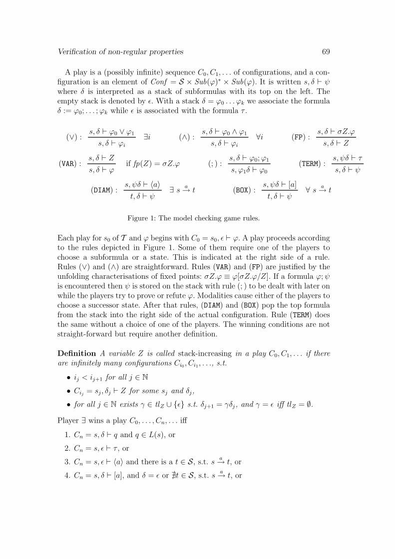
Verification of non-regular properties 69
A play is a (possibly infinite) sequence C0, C1, . . . of configurations, and a con-figuration is an element of Conf = S × Sub(ϕ)∗ × Sub(ϕ). It is written s, δ ⊢ ψwhere δ is interpreted as a stack of subformulas with its top on the left. Theempty stack is denoted by ǫ. With a stack δ = ϕ0 . . . ϕk we associate the formulaδ := ϕ0; . . . ;ϕk while ǫ is associated with the formula τ .
(∨) :s, δ ⊢ ϕ0 ∨ ϕ1
s, δ ⊢ ϕi
∃i (∧) :s, δ ⊢ ϕ0 ∧ ϕ1
s, δ ⊢ ϕi
∀i (FP) :s, δ ⊢ σZ.ϕs, δ ⊢ Z
(VAR) :s, δ ⊢ Zs, δ ⊢ ϕ
if fp(Z) = σZ.ϕ (; ) :s, δ ⊢ ϕ0;ϕ1
s, ϕ1δ ⊢ ϕ0
(TERM) :s, ψδ ⊢ τs, δ ⊢ ψ
(DIAM) :s, ψδ ⊢ 〈a〉t, δ ⊢ ψ
∃ s a→ t (BOX) :s, ψδ ⊢ [a]
t, δ ⊢ ψ∀ s a→ t
Figure 1: The model checking game rules.
Each play for s0 of T and ϕ begins with C0 = s0, ǫ ⊢ ϕ. A play proceeds accordingto the rules depicted in Figure 1. Some of them require one of the players tochoose a subformula or a state. This is indicated at the right side of a rule.Rules (∨) and (∧) are straightforward. Rules (VAR) and (FP) are justified by theunfolding characterisations of fixed points: σZ.ϕ ≡ ϕ[σZ.ϕ/Z]. If a formula ϕ;ψis encountered then ψ is stored on the stack with rule (; ) to be dealt with later onwhile the players try to prove or refute ϕ. Modalities cause either of the players tochoose a successor state. After that rules, (DIAM) and (BOX) pop the top formulafrom the stack into the right side of the actual configuration. Rule (TERM) doesthe same without a choice of one of the players. The winning conditions are notstraight-forward but require another definition.
Definition A variable Z is called stack-increasing in a play C0, C1, . . . if thereare infinitely many configurations Ci0, Ci1, . . ., s.t.
• ij < ij+1 for all j ∈ N
• Cij = sj , δj ⊢ Z for some sj and δj,
• for all j ∈ N exists γ ∈ tlZ ∪ {ǫ} s.t. δj+1 = γδj, and γ = ǫ iff tlZ = ∅.
Player ∃ wins a play C0, . . . , Cn, . . . iff
1. Cn = s, δ ⊢ q and q ∈ L(s), or
2. Cn = s, ǫ ⊢ τ , or
3. Cn = s, ǫ ⊢ 〈a〉 and there is a t ∈ S, s.t. sa→ t, or
4. Cn = s, δ ⊢ [a], and δ = ǫ or ∄t ∈ S, s.t. sa→ t, or
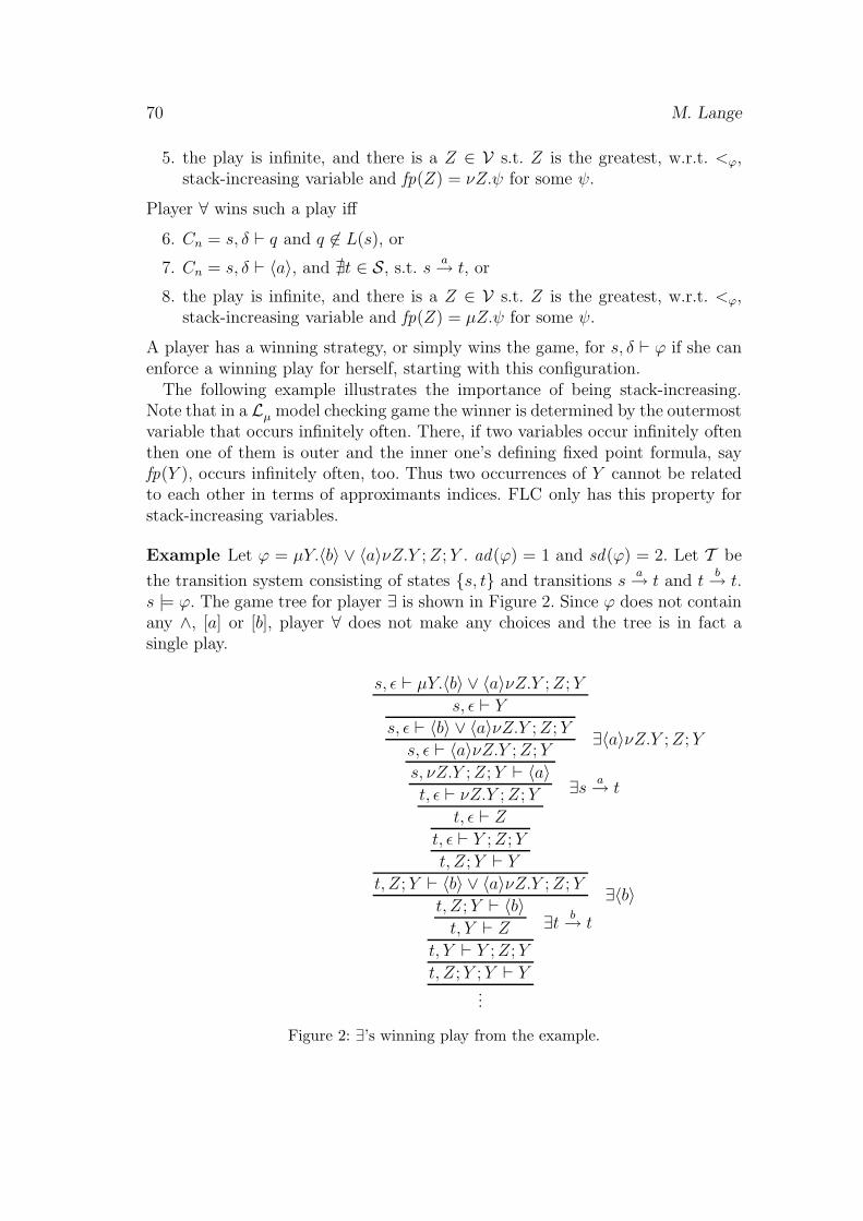
70 M. Lange
5. the play is infinite, and there is a Z ∈ V s.t. Z is the greatest, w.r.t. <ϕ,stack-increasing variable and fp(Z) = νZ.ψ for some ψ.
Player ∀ wins such a play iff
6. Cn = s, δ ⊢ q and q 6∈ L(s), or
7. Cn = s, δ ⊢ 〈a〉, and ∄t ∈ S, s.t. sa→ t, or
8. the play is infinite, and there is a Z ∈ V s.t. Z is the greatest, w.r.t. <ϕ,stack-increasing variable and fp(Z) = µZ.ψ for some ψ.
A player has a winning strategy, or simply wins the game, for s, δ ⊢ ϕ if she canenforce a winning play for herself, starting with this configuration.
The following example illustrates the importance of being stack-increasing.Note that in a Lµ model checking game the winner is determined by the outermostvariable that occurs infinitely often. There, if two variables occur infinitely oftenthen one of them is outer and the inner one’s defining fixed point formula, sayfp(Y ), occurs infinitely often, too. Thus two occurrences of Y cannot be relatedto each other in terms of approximants indices. FLC only has this property forstack-increasing variables.
Example Let ϕ = µY.〈b〉 ∨ 〈a〉νZ.Y ;Z;Y . ad(ϕ) = 1 and sd(ϕ) = 2. Let T be
the transition system consisting of states {s, t} and transitions sa→ t and t
b→ t.s |= ϕ. The game tree for player ∃ is shown in Figure 2. Since ϕ does not containany ∧, [a] or [b], player ∀ does not make any choices and the tree is in fact asingle play.
s, ǫ ⊢ µY.〈b〉 ∨ 〈a〉νZ.Y ;Z;Y
s, ǫ ⊢ Ys, ǫ ⊢ 〈b〉 ∨ 〈a〉νZ.Y ;Z;Y ∃〈a〉νZ.Y ;Z;Ys, ǫ ⊢ 〈a〉νZ.Y ;Z;Y
s, νZ.Y ;Z;Y ⊢ 〈a〉∃s a→ tt, ǫ ⊢ νZ.Y ;Z;Y
t, ǫ ⊢ Zt, ǫ ⊢ Y ;Z;Y
t, Z;Y ⊢ Yt, Z;Y ⊢ 〈b〉 ∨ 〈a〉νZ.Y ;Z;Y ∃〈b〉
t, Z;Y ⊢ 〈b〉∃t b→ tt, Y ⊢ Z
t, Y ⊢ Y ;Z;Y
t, Z;Y ;Y ⊢ Y...
Figure 2: ∃’s winning play from the example.

Verification of non-regular properties 71
Both Y and Z occur infinitely often in the play. However, neither fp(Y ) norfp(Z) does. Note that Z <ϕ Y . Y gets “fulfilled” each time it is replaced by itsdefining fixed point formula, but reproduced by Z. On the other hand, Y doesnot start a new computation of fp(Z) each time it is reproduced. But Y is notstack-increasing whereas Z is. And Z denotes a greatest fixed point, thereforeplayer ∃ wins this play.
4. Results on FLC(’s model checking problem)
Theorem (Decidability) FLC’s satisfiability checking problem is undecidable;FLC does not have the finite model property; its model checking problem is de-cidable for finite structures [7]; but undecidable for normed deterministic BPAalready [4].
Theorem (Expressiveness) On linear structures (infinite words) the class ofFLC-definable languages coincides with the class of alternating context-free gram-mars (with a parity acceptance condition) [3].
Theorem (Complexity) FLC’s model checking problem is in EXPTIME andPSPACE-hard [5], even for a fixed formula [6]. For formulas with fixed alternation(and sequential) depth, the model checking problem is in PSPACE.
Obviously, the complexity results refer to finite structures only.
References
[1] D. Janin and I. Walukiewicz. On the expressive completeness of the propositio-nal µ-calculus with respect to monadic second order logic. In U. Montanari andV. Sassone, editors, Proc. 7th Conf. on Concurrency Theory, CONCUR’96,volume 1119 of LNCS, pages 263–277, Pisa, Italy, August 1996. Springer.
[2] D. Kozen. Results on the propositional µ-calculus. TCS, 27:333–354, Decem-ber 1983.
[3] M. Lange. Alternating context-free languages and linear time µ-calculus withsequential composition. In P. Panangaden and U. Nestmann, editors, Proc.9th Workshop on Expressiveness in Concurrency, EXPRESS’02, volume 68.2of ENTCS, pages 71–87, Brno, Czech Republic, August 2002. Elsevier.
[4] M. Lange. Local model checking games for fixed point logic with chop. InL. Brim, P. Jancar, M. Kretınsky, and A. Kucera, editors, Proc. 13th Conf.on Concurrency Theory, CONCUR’02, volume 2421 of LNCS, pages 240–254,Brno, Czech Republic, August 2002. Springer.
[5] M. Lange and C. Stirling. Model checking fixed point logic with chop. InM. Nielsen and U. H. Engberg, editors, Proc. 5th Conf. on Foundations of
72 M. Lange
Software Science and Computation Structures, FOSSACS’02, volume 2303 ofLNCS, pages 250–263, Grenoble, France, April 2002. Springer.
[6] M. Muller-Olm. private communication.
[7] M. Muller-Olm. A modal fixpoint logic with chop. In C. Meinel and S. Ti-son, editors, Proc. 16th Symp. on Theoretical Aspects of Computer Science,STACS’99, volume 1563 of LNCS, pages 510–520, Trier, Germany, 1999.Springer.
[8] C. Stirling. Local model checking games. In I. Lee and S. A. Smolka, editors,Proc. 6th Conf. on Concurrency Theory, CONCUR’95, volume 962 of LNCS,pages 1–11, Berlin, Germany, August 1995. Springer.
[9] A. Tarski. A lattice-theoretical fixpoint theorem and its application. PacificJ.Math., 5:285–309, 1955.

A HIERARCHY OF MSC LANGUAGES
Benedikt Bollig
Lehrstuhl fur Informatik IIAachen University of Technology
Germanye-mail: [email protected]
and
Martin Leucker
IT departmentUppsala University
Swedene-mail: [email protected]
ABSTRACT
Introduction A common design practice when developing communicating sys-tems is to start with drawing scenarios showing the intended interaction of thesystem to be. The standardized notion of message sequence charts (MSCs, [3])is widely used in industry to formalize such typical behaviours.
A message sequence chart defines a set of processes and a set of communicationactions between these processes. In the visual representation of an MSC, pro-cesses are drawn as vertical lines and interpreted as time lines. A labelled arrowfrom one line to a second corresponds to the communication event of sending thelabelling value from the first process to the second. Collections of MSCs are usedto capture the scenarios that a designer might want the system to follow or toavoid. Figure 1 shows three MSCs.
To support the detection of errors and to validate the intended design, formalanalysis techniques for MSCs are of great value. One important question that hasbeen studied recently is model checking MSC specifications. The motivation isthat a designer could specify the scenarios using a collection of MSCs and verifythem against certain requirements.
73
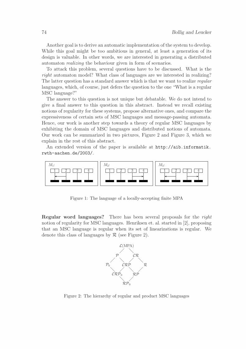
74 Bollig and Leucker
Another goal is to derive an automatic implementation of the system to develop.While this goal might be too ambitious in general, at least a generation of itsdesign is valuable. In other words, we are interested in generating a distributedautomaton realizing the behaviour given in form of scenarios.
To attack this problem, several questions have to be discussed. What is theright automaton model? What class of languages are we interested in realizing?The latter question has a standard answer which is that we want to realize regularlanguages, which, of course, just defers the question to the one “What is a regularMSC language?”
The answer to this question is not unique but debatable. We do not intend togive a final answer to this question in this abstract. Instead we recall existingnotions of regularity for these systems, propose alternative ones, and compare theexpressiveness of certain sets of MSC languages and message-passing automata.Hence, our work is another step towards a theory of regular MSC languages byexhibiting the domain of MSC languages and distributed notions of automata.Our work can be summarized in two pictures, Figure 2 and Figure 3, which weexplain in the rest of this abstract.
An extended version of the paper is available at http://aib.informatik.
rwth-aachen.de/2003/.
1 2 3 4
M1:
1 2 3 4
M2:
1 2 3 4
M3:
Figure 1: The language of a locally-accepting finite MPA
Regular word languages? There has been several proposals for the rightnotion of regularity for MSC languages. Henriksen et. al. started in [2], proposingthat an MSC language is regular when its set of linearizations is regular. Wedenote this class of languages by R (see Figure 2).
RP0
CRP0
P0
RP
CRP
P
R
CR
L(MPA)
Figure 2: The hierarchy of regular and product MSC languages
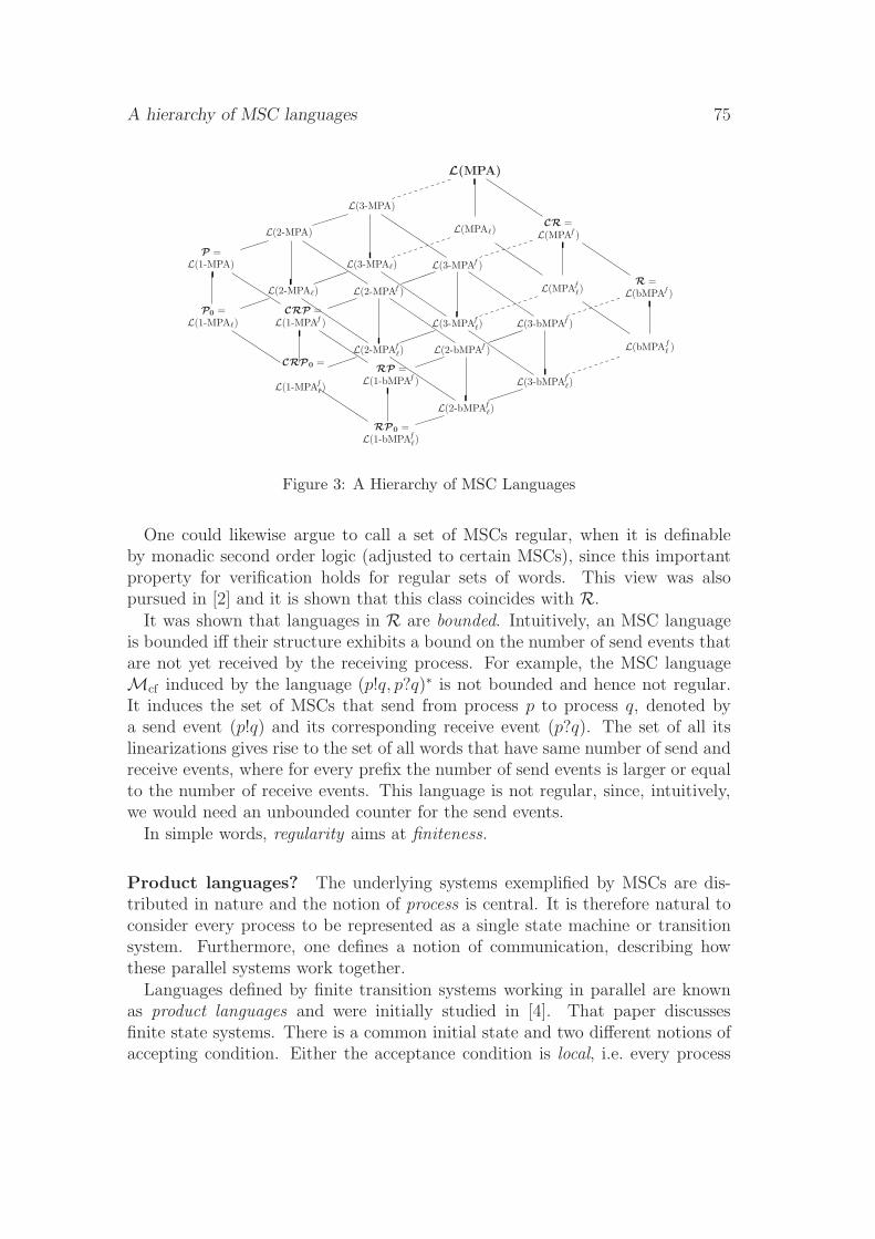
A hierarchy of MSC languages 75
L(MPAℓ)
L(MPAfℓ)
L(bMPAfℓ )
RP0 =L(1-bMPAf
ℓ)
CRP0 =
L(1-MPAfℓ)
P0 =L(1-MPAℓ)
RP =L(1-bMPAf )
CRP =L(1-MPAf )
P =L(1-MPA)
R =L(bMPAf )
CR =L(MPAf )
L(MPA)
L(2-MPAfℓ)
L(3-MPAfℓ)
L(2-MPAf )
L(3-MPAf )
L(2-bMPAfℓ)
L(3-bMPAfℓ)
L(2-bMPAf )
L(3-bMPAf )
L(2-MPAℓ)
L(3-MPAℓ)
L(2-MPA)
L(3-MPA)
Figure 3: A Hierarchy of MSC Languages
One could likewise argue to call a set of MSCs regular, when it is definableby monadic second order logic (adjusted to certain MSCs), since this importantproperty for verification holds for regular sets of words. This view was alsopursued in [2] and it is shown that this class coincides with R.
It was shown that languages in R are bounded. Intuitively, an MSC languageis bounded iff their structure exhibits a bound on the number of send events thatare not yet received by the receiving process. For example, the MSC languageMcf induced by the language (p!q, p?q)∗ is not bounded and hence not regular.It induces the set of MSCs that send from process p to process q, denoted bya send event (p!q) and its corresponding receive event (p?q). The set of all itslinearizations gives rise to the set of all words that have same number of send andreceive events, where for every prefix the number of send events is larger or equalto the number of receive events. This language is not regular, since, intuitively,we would need an unbounded counter for the send events.
In simple words, regularity aims at finiteness.
Product languages? The underlying systems exemplified by MSCs are dis-tributed in nature and the notion of process is central. It is therefore natural toconsider every process to be represented as a single state machine or transitionsystem. Furthermore, one defines a notion of communication, describing howthese parallel systems work together.
Languages defined by finite transition systems working in parallel are knownas product languages and were initially studied in [4]. That paper discussesfinite state systems. There is a common initial state and two different notions ofaccepting condition. Either the acceptance condition is local, i.e. every process
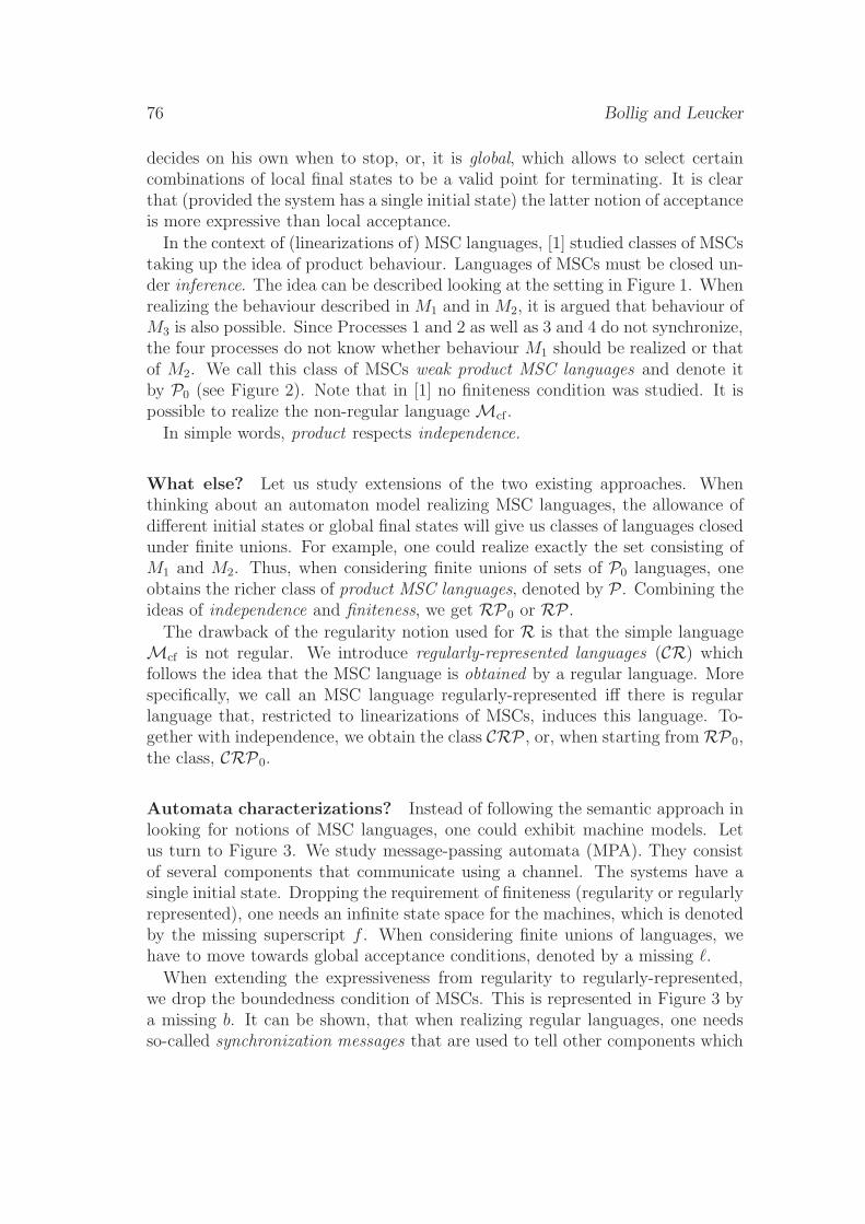
76 Bollig and Leucker
decides on his own when to stop, or, it is global, which allows to select certaincombinations of local final states to be a valid point for terminating. It is clearthat (provided the system has a single initial state) the latter notion of acceptanceis more expressive than local acceptance.
In the context of (linearizations of) MSC languages, [1] studied classes of MSCstaking up the idea of product behaviour. Languages of MSCs must be closed un-der inference. The idea can be described looking at the setting in Figure 1. Whenrealizing the behaviour described in M1 and in M2, it is argued that behaviour ofM3 is also possible. Since Processes 1 and 2 as well as 3 and 4 do not synchronize,the four processes do not know whether behaviour M1 should be realized or thatof M2. We call this class of MSCs weak product MSC languages and denote itby P0 (see Figure 2). Note that in [1] no finiteness condition was studied. It ispossible to realize the non-regular language Mcf .
In simple words, product respects independence.
What else? Let us study extensions of the two existing approaches. Whenthinking about an automaton model realizing MSC languages, the allowance ofdifferent initial states or global final states will give us classes of languages closedunder finite unions. For example, one could realize exactly the set consisting ofM1 and M2. Thus, when considering finite unions of sets of P0 languages, oneobtains the richer class of product MSC languages, denoted by P. Combining theideas of independence and finiteness, we get RP0 or RP .
The drawback of the regularity notion used for R is that the simple languageMcf is not regular. We introduce regularly-represented languages (CR) whichfollows the idea that the MSC language is obtained by a regular language. Morespecifically, we call an MSC language regularly-represented iff there is regularlanguage that, restricted to linearizations of MSCs, induces this language. To-gether with independence, we obtain the class CRP , or, when starting from RP0,the class, CRP0.
Automata characterizations? Instead of following the semantic approach inlooking for notions of MSC languages, one could exhibit machine models. Letus turn to Figure 3. We study message-passing automata (MPA). They consistof several components that communicate using a channel. The systems have asingle initial state. Dropping the requirement of finiteness (regularity or regularlyrepresented), one needs an infinite state space for the machines, which is denotedby the missing superscript f . When considering finite unions of languages, wehave to move towards global acceptance conditions, denoted by a missing ℓ.
When extending the expressiveness from regularity to regularly-represented,we drop the boundedness condition of MSCs. This is represented in Figure 3 bya missing b. It can be shown, that when realizing regular languages, one needsso-called synchronization messages that are used to tell other components which
A hierarchy of MSC languages 77
transition was taken. We show that the more of these messages are allowed, themore expressive power we have. The restriction to n synchronization messages isdescribed by a preceding n- in Figure 3.
References
[1] R. Alur, K. Etessami, and M. Yannakakis. Inference of message sequencecharts. In 22nd International Conference on Software Engineering, pages304–313, 2000.
[2] J. G. Henriksen, M. Mukund, K. Narayan Kumar, and P. S. Thiagarajan.Regular collections of message sequence charts. In Proceedings of 25th In-ternational Symposium on Mathematical Foundations of Computer Science(MFCS’2000), volume 1893 of Lecture Notes in Computer Science, pages 405–414. Springer, 2000.
[3] ITU-TS. ITU-TS Recommendation Z.120: Message Sequence Chart 1999(MSC99). Technical report, ITU-TS, Geneva, 1999.
[4] P. S. Thiagarajan. A trace consistent subset of PTL. In Insup Lee andScott A. Smolka, editors, Proceedings of the 6th International Conference onConcurrency Theory (CONCUR’95), volume 962 of Lecture Notes in Com-puter Science, pages 438–452, Philadelphia, Pennsylvania, 21–24 August 1995.Springer.
MINIMIZING FINITE AUTOMATA IS
COMPUTATIONALLY HARD
Andreas Malcher
Institut fur Informatik, Johann Wolfgang Goethe-UniversitatD-60054 Frankfurt am Main, Germany
e-mail: [email protected]
ABSTRACT
It is known that deterministic finite automata (DFAs) can be algorithmically min-imized, i.e., a DFA M can be converted to an equivalent DFA M ′ which has aminimal number of states. The minimization can be done efficiently [5]. On theother hand, it is known that unambiguous finite automata (UFAs) and nondeter-ministic finite automata (NFAs) can be algorithmically minimized too, but theirminimization problems turn out to be NP-complete and PSPACE-complete, respec-tively [7]. In this paper, the time complexity of the minimization problem for tworestricted types of finite automata is investigated. These automata are nearly deter-ministic, since they only allow a small amount of nondeterminism to be used. Themain result is that the minimization problems for these models are computationallyhard, namely NP-complete. Hence, even the slightest extension of the deterministicmodel towards a nondeterministic one, e.g., allowing at most one nondeterministicmove in every accepting computation or allowing two initial states instead of one,results in computationally intractable minimization problems.
Keywords: Finite automata, limited nondeterminism, minimization, NP-complete.
1. Introduction
Finite automata are a well-investigated concept in theoretical computer sciencewith a wide range of applications such as lexical analysis, pattern matching, orprotocol specification in distributed systems. Due to time and space constraintsit is often very useful to provide minimal or at least succinct descriptions ofsuch automata. Deterministic finite automata (DFAs) and their correspondinglanguage class, the set of regular languages, possess many nice properties suchas, for example, closure under many language operations and many decidablequestions. In addition, most of the decidability questions for DFAs, such asmembership, emptiness, or equivalence, are efficiently solvable (cf. Sect. 5.2 in
78

Minimizing finite automata is computationally hard 79
[12]). Furthermore, in [5] a minimization algorithm for DFAs is provided workingin time O(n logn), where n denotes the number of states of the given DFA.
It is known that both nondeterministic finite automata (NFAs) and DFAs ac-cept the set of regular languages, but NFAs can achieve exponentially savings insize when compared to DFAs [10]. Unfortunately, certain decidability questions,which are solvable in polynomial time for DFAs, are computationally hard forNFAs such as equivalence, inclusion, or universality [11, 12]. Furthermore, theminimization of NFAs is proven to be PSPACE-complete in [7]. In the latter pa-per, it is additionally shown that unambiguous finite automata (UFAs) have anNP-complete minimization problem.
Therefore, we can summarize that determinism permits efficient solutionswhereas the use of nondeterminism often makes solutions computationally in-tractable. Thus, one might ask what amount of nondeterminism is necessary tomake things computationally hard, or, in other words, what amount of nondeter-minism may be allowed so that efficiency is preserved.
Measures of nondeterminism in finite automata were first considered in [9] and[1] where the relation between the amount of nondeterminism of an NFA andthe succinctness of its description is studied. Here, we look at computationalcomplexity aspects of NFAs with a fixed finite amount of nondeterminism. Inparticular, these NFAs are restricted such that within every accepting computa-tion at most a fixed number of nondeterministic moves is allowed to be chosen.It is easily observed that certain decidability questions then become solvable inpolynomial time in contrast to arbitrary NFAs. However, the minimization prob-lem for such NFAs is proven to be NP-complete.
We further investigate a model where the nondeterminism used is not only re-stricted to a fixed finite number of nondeterministic moves, but is additionally cutdown such that only the first move is allowed to be a nondeterministic one. Hencewe come to DFAs with multiple initial states (MDFAs) which were introducedin [4] and recently studied in [8] and [2]. We will show that the minimizationproblem of such MDFAs is NP-complete even if only two initial states are given.In analogy to NFAs with fixed finite branching, certain decidability questions canbe shown to be efficiently solvable.
2. Definitions
Concerning the definitions of NFAs with finite branching and MDFAs we followthe notations introduced in [1] and [8].
A nondeterministic finite automaton over Σ is a tuple M = (Q,Σ, δ, q0, F ),with Q a finite set of states, q0 ∈ Q the initial state, F ⊆ Q the set of acceptingstates, and δ a function from Q×Σ to 2Q. A move of M is a triple µ = (p, a, q) ∈Q × Σ × Q with q ∈ δ(p, a). A computation for w = w1w2 . . . wn ∈ Σ∗ is asequence of moves µ1µ2 . . . µn where µi = (qi−1, wi, qi) with 1 ≤ i ≤ n. It is anaccepting computation if qn ∈ F . The language accepted by M is T (M) = {w ∈
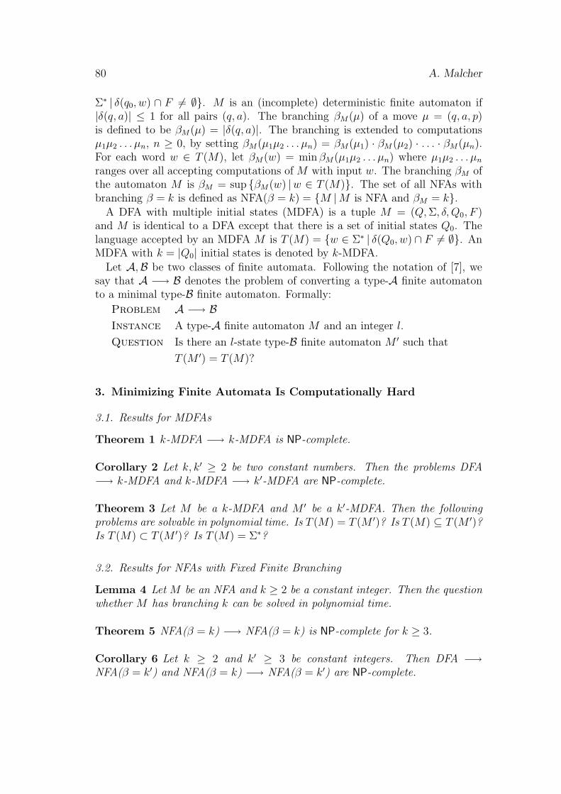
80 A. Malcher
Σ∗ | δ(q0, w) ∩ F 6= ∅}. M is an (incomplete) deterministic finite automaton if|δ(q, a)| ≤ 1 for all pairs (q, a). The branching βM(µ) of a move µ = (q, a, p)is defined to be βM(µ) = |δ(q, a)|. The branching is extended to computationsµ1µ2 . . . µn, n ≥ 0, by setting βM(µ1µ2 . . . µn) = βM(µ1) · βM (µ2) · . . . · βM(µn).For each word w ∈ T (M), let βM(w) = min βM(µ1µ2 . . . µn) where µ1µ2 . . . µn
ranges over all accepting computations of M with input w. The branching βM ofthe automaton M is βM = sup {βM(w) |w ∈ T (M)}. The set of all NFAs withbranching β = k is defined as NFA(β = k) = {M |M is NFA and βM = k}.
A DFA with multiple initial states (MDFA) is a tuple M = (Q,Σ, δ, Q0, F )and M is identical to a DFA except that there is a set of initial states Q0. Thelanguage accepted by an MDFA M is T (M) = {w ∈ Σ∗ | δ(Q0, w) ∩ F 6= ∅}. AnMDFA with k = |Q0| initial states is denoted by k-MDFA.
Let A,B be two classes of finite automata. Following the notation of [7], wesay that A −→ B denotes the problem of converting a type-A finite automatonto a minimal type-B finite automaton. Formally:
Problem A −→ BInstance A type-A finite automaton M and an integer l.
Question Is there an l-state type-B finite automaton M ′ such that
T (M ′) = T (M)?
3. Minimizing Finite Automata Is Computationally Hard
3.1. Results for MDFAs
Theorem 1 k-MDFA −→ k-MDFA is NP-complete.
Corollary 2 Let k, k′ ≥ 2 be two constant numbers. Then the problems DFA−→ k-MDFA and k-MDFA −→ k′-MDFA are NP-complete.
Theorem 3 Let M be a k-MDFA and M ′ be a k′-MDFA. Then the followingproblems are solvable in polynomial time. Is T (M) = T (M ′)? Is T (M) ⊆ T (M ′)?Is T (M) ⊂ T (M ′)? Is T (M) = Σ∗?
3.2. Results for NFAs with Fixed Finite Branching
Lemma 4 Let M be an NFA and k ≥ 2 be a constant integer. Then the questionwhether M has branching k can be solved in polynomial time.
Theorem 5 NFA(β = k) −→ NFA(β = k) is NP-complete for k ≥ 3.
Corollary 6 Let k ≥ 2 and k′ ≥ 3 be constant integers. Then DFA −→NFA(β = k′) and NFA(β = k) −→ NFA(β = k′) are NP-complete.
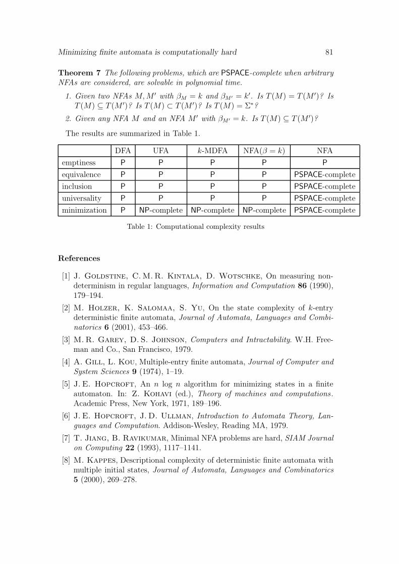
Minimizing finite automata is computationally hard 81
Theorem 7 The following problems, which are PSPACE-complete when arbitraryNFAs are considered, are solvable in polynomial time.
1. Given two NFAs M,M ′ with βM = k and βM ′ = k′. Is T (M) = T (M ′)? IsT (M) ⊆ T (M ′)? Is T (M) ⊂ T (M ′)? Is T (M) = Σ∗?
2. Given any NFA M and an NFA M ′ with βM ′ = k. Is T (M) ⊆ T (M ′)?
The results are summarized in Table 1.
DFA UFA k-MDFA NFA(β = k) NFA
emptiness P P P P P
equivalence P P P P PSPACE-complete
inclusion P P P P PSPACE-complete
universality P P P P PSPACE-complete
minimization P NP-complete NP-complete NP-complete PSPACE-complete
Table 1: Computational complexity results
References
[1] J. Goldstine, C.M.R. Kintala, D. Wotschke, On measuring non-determinism in regular languages, Information and Computation 86 (1990),179–194.
[2] M. Holzer, K. Salomaa, S. Yu, On the state complexity of k-entrydeterministic finite automata, Journal of Automata, Languages and Combi-natorics 6 (2001), 453–466.
[3] M.R. Garey, D. S. Johnson, Computers and Intractability. W.H. Free-man and Co., San Francisco, 1979.
[4] A. Gill, L. Kou, Multiple-entry finite automata, Journal of Computer andSystem Sciences 9 (1974), 1–19.
[5] J. E. Hopcroft, An n log n algorithm for minimizing states in a finiteautomaton. In: Z. Kohavi (ed.), Theory of machines and computations.Academic Press, New York, 1971, 189–196.
[6] J. E. Hopcroft, J. D. Ullman, Introduction to Automata Theory, Lan-guages and Computation. Addison-Wesley, Reading MA, 1979.
[7] T. Jiang, B. Ravikumar, Minimal NFA problems are hard, SIAM Journalon Computing 22 (1993), 1117–1141.
[8] M. Kappes, Descriptional complexity of deterministic finite automata withmultiple initial states, Journal of Automata, Languages and Combinatorics5 (2000), 269–278.

82 A. Malcher
[9] C. M.R. Kintala, D. Wotschke, Amounts of nondeterminism in finiteautomata, Acta Informatica 13 (1980), 199–204.
[10] A. R. Meyer, M. J. Fischer, Economy of descriptions by automata,grammars, and formal systems. In: IEEE Symposium on Foundations ofComputer Science, 1971, 188–191.
[11] L. Stockmeyer, A.R. Meyer, Word problems requiring exponentialtime: preliminary report. In: Fifth Annual ACM Symposium on Theoryof Computing , 1973, 1–9.
[12] S. Yu, Regular languages. In: G. Rozenberg, A. Salomaa (eds.), Hand-book of Formal Languages Vol. 1. Springer-Verlag, Berlin, 1997, 41–110.
HIERARCHIES OF WEAKLY MONOTONERESTARTING AUTOMATA
Frantisek Mraz1
Department of Computer Science, Charles UniversityMalostranske nam. 25, 118 00 Praha 1, Czech Republic
e-mail: [email protected]
and
Friedrich Otto2
Fachbereich Mathematik/Informatik, Universitat Kassel34109 Kassel, Germany
e-mail: [email protected]
ABSTRACT
It is known that the weakly monotone restarting automata accept exactly the grow-ing context-sensitive langauges. We introduce a measure on the degree of weakmonotonicity and show that the language classes obtained in this way form stricthierarchies for the various types of deterministic and nondeterministic restartingautomata without auxiliary symbols.
Keywords: Restarting automata, growing context-sensitive languages, degree ofweak monotonicity.
1. Introduction
The motivation for introducing the restarting automaton in [2] was the desireto model the so-called analysis by reduction of natural languages [12, 13]. Thisanalysis consists of a stepwise simplification of a sentence in such a way that thesyntactical correctness or incorrectness of the sentence is not affected. After afinite number of steps either a correct simple sentence is obtained, or an error is
2The first author was partially supported by the Grant Agency of the Czech Republic,Grant-No. 201/02/1456, and the Grant Agency of Charles University, Grant No. 300/2002/A-INF/MFF.
2The work of the second author was partially supported by a grant from the DeutscheForschungsgemeinschaft (DFG).
83

84 F. Mraz, F. Otto
detected. It turned out that the restarting automaton thus obtained can handlea class of languages that is much broader than the class CFL of context-freelanguages.
A restarting automaton, or RRWW-automaton, M is a device with a finitestate control and a read/write window of fixed size. This window moves fromleft to right along a tape containing a string delimited by sentinels until M ’scontrol decides (nondeterministically) that the contents of the window should berewritten by some shorter string. After a rewrite, M continues to move its windowto the right until it either halts and accepts, or halts and rejects, which meansthat it has reached a configuration from which it cannot continue, or restarts,that is, it moves its window to the leftmost position, enters the initial state, andcontinues with the computation.
Also some restricted variants of the restarting automaton have been considered.First, there are the deterministic variants. Then there are those variants thatare allowed to only use the letters from the input alphabet, while in general arestarting automaton can use a finite number of auxiliary symbols in its rewritesteps. Further, a monotonicity property was introduced for RRWW-automata,and it was shown that the monotone RRWW-automata (with auxiliary symbols)characterize the class CFL, and that various restricted versions of deterministicmonotone RRWW-automata (with or without auxiliary symbols) characterize theclass DCFL of deterministic context-free languages [3].
In [5, 7] the class CRL of Church-Rosser languages was introduced motivated bythe fact that membership for these languages is decidable in linear time. In [10] itwas then shown that the deterministic RRWW-automata (with auxiliary symbols)give another characterization of CRL. For the growing context-sensitive languagesGCSL [1], which can be seen as the nondeterministic variants of the Church-Rosserlanguages [8], it was observed in [9] that they form a proper subclass of the classL(RRWW) of languages that are accepted by RRWW-automata.
In order to obtain a characterization of GCSL in terms of restarting automata,a relaxation of the monotonicity condition for RRWW-automata was introducedin [4]. Let c be a non-negative integer. An RRWW-automaton M is called weaklyc-monotone if in any two consecutive rewrite steps of any computation of M theplaces of rewriting can increase their distances from the right end of the tape byat most c positions. An RRWW-automaton M is called weakly monotone if thereexists a non-negative integer c such that M is weakly c-monotone. The weaklymonotone RRWW-automata (with auxiliary symbols) recognize exactly GCSL [4].For a recent survey on the restarting automata see [11].
Here we study the influence of the degree of weak monotonicity on the ex-pressive power of the various models of restarting automata. We focus on therestarting automata with the most transparent computations – those withoutauxiliary symbols. Further motivation for studying weak monotonicity comesfrom linguistics. The degree of weak monotonicity is a measure of across howmany symbols (words of a sentence) already read before a reader must step back

Hierarchies of weakly monotone restarting automata 85
to the left during an analysis of a sentence in a certain (natural) language.
2. Definitions
A restarting automaton, RRWW-automaton for short, is a one-tape machine thatis described by an 8-tuple M = (Q,Σ,Γ, c, $, q0, k, δ), where Q is the finite setof states, Σ is the finite input alphabet, Γ is the finite tape alphabet containingΣ, c, $ 6∈ Γ are the markers for the left and right border of the work space,respectively, q0 ∈ Q is the initial state, k ≥ 1 is the size of the read/writewindow, and
δ : Q× PC(k) → P((Q× ({MVR} ∪ PC(k−1))) ∪ {Restart,Accept})
is the transition relation. Here P(S) denotes the powerset of the set S, and
PC(k) := (c·Γk−1) ∪ Γk ∪ (Γ≤k−1·$) ∪ (c·Γ≤k−2·$)
is the set of possible contents of the read/write-window of M , where Γ≤n :=n⋃
i=0Γi,
and PC(k−1) is defined analogously.
The transition relation describes four different types of transition steps:
1. A move-right step is of the form (q′,MVR) ∈ δ(q, u), where q, q′ ∈ Q andu ∈ PC(k), u 6= $. If M is in state q and sees the string u in its read/write-window, then this move-right step causes M to shift the read/write-windowone position to the right and to enter state q′.
2. A rewrite step is of the form (q′, v) ∈ δ(q, u), where q, q′ ∈ Q, u ∈ PC(k),u 6= $, and v ∈ PC(k−1) such that |v| < |u|. It causes M to replace thecontents u of the read/write-window by the string v and to enter state q′.Further, the read/write-window is placed immediately to the right of thestring v. However, some additional restrictions apply in that the bordermarkers c and $ must not disappear from the tape nor that new occurrencesof these markers are created. Further, the read/write-window must not moveacross the right border marker $.
3. A restart step is of the form Restart ∈ δ(q, u), where q ∈ Q and u ∈ PC(k).It causes M to move its read/write-window to the left end of the tape, sothat the first symbol it sees is the left border marker c, and to reenter theinitial state q0.
4. An accept step is of the form Accept ∈ δ(q, u), where q ∈ Q and u ∈ PC(k).It causes M to halt and accept.
Obviously, each computation of M proceeds in cycles. Starting from an initialconfiguration q0cw$, the head moves right, while move-right and rewrite stepsare executed until finally a restart step takes M back into a configuration of the
86 F. Mraz, F. Otto
form q0cw1$. It is required that in each such cycle exactly one rewrite step isexecuted. By ⊢c
M we denote the execution of a complete cycle. As by a rewritestep the contents of the tape is shortened, only a linear number of cycles can beexecuted within any computation. That part of a computation of M that followsafter the execution of the last restart is called the tail of the computation. Itcontains at most a single application of a rewrite step.
An input w ∈ Σ∗ is accepted by M , if there exists a computation of M whichstarts with the initial configuration q0cw$, and which finally ends with executingan accept step. By L(M) we denote the language accepted by M , and L(RRWW)will denote the class of languages that are accepted by RRWW-automata.
In [3] a notion of monotonicity is considered for restarting automata. Let M bean RRWW-automaton. Each computation of M can be described by a sequenceof cycles C1, C2 . . . , Cn, where C1 starts with an initial configuration of M , andCn is the last cycle, which is followed by the tail of the computation. Eachcycle Ci contains a unique configuration of the form cxuy$ such that u → v isthe rewrite step applied during this cycle. By Dr(Ci) we denote the r-distance|y$| of this cycle. The sequence of cycles C1, C2, . . . , Cn is called monotone ifDr(C1) ≥ Dr(C2) ≥ . . . ≥ Dr(Cn) holds, and the RRWW-automaton M is calledmonotone if all its computations are monotone.
In [3] it is shown that all variants of deterministic monotone restarting au-tomata accept exactly the deterministic context-free languages. For the nonde-terministic restarting automata it turned out that the use of auxiliary symbols isnecessary to obtain a characterization of the class of context-free languages.
In order to derive a characterization of the class GCSL of growing context-sensitive languages in terms of restarting automata, the notion of weak mono-tonicity was introduced in [4]. LetM be an R(R)WW-automaton, and let c ≥ 0 bean integer. We say that a sequence of cycles C1, C2, . . . , Cn is weakly c-monotone,if Dr(Ci+1) ≤ Dr(Ci) + c holds for all i = 1, 2, . . . , n− 1. An RRWW-automatonM is called weakly c-monotone if all its computations are weakly c-monotone.Further, we say that M is weakly monotone, if there exists a constant c ≥ 0 suchthat M is weakly c-monotone. The prefixes w(c)mon- and wmon- are used todenote the corresponding classes of restarting automata.
For deterministic RRWW-automata we have the following observation.
Lemma 1 Each deterministic RRWW-automaton with window size k is weaklyj-monotone for some j ≤ k − 2.
Thus, for deterministic R(R)WW-automata the above weak monotonicity con-dition is always satisfied, that is,
CRL = L(det-wmon-RWW) = L(det-wmon-RRWW).
Hence, it is only for the various nondeterministic restarting automata that these

Hierarchies of weakly monotone restarting automata 87
additional restrictions make a difference. In [4] it is shown that
GCSL = L(wmon-RWW) = L(wmon-RRWW) ⊂ L(RWW),
where the inclusion is known to be proper.
3. Hierarchies with respect to the degree of weak monotonicity
Here we are interested in the influence of the degree of weak monotonicity onthe expressive power of the various types of restarting automata. It can beshown by specifically chosen example languages that the expressive power of thevarious types of deterministic and nondeterministic restarting automata withoutauxiliary symbols strictly increases when the degree of weak monotonicity grows.
Theorem 2 [6] For each i ≥ 0 and for each X ∈ {R,RR,RW,RRW},(a) L(det-w(i)mon−X) ⊆ L(det-w(i + 1 )mon−X).
(b) L(w(i)mon−X) ⊆ L(w(i + 1 )mon−X).
Further, it can be shown that these hierarchies differ pairwise from each other.These results can best be presented by the following diagram, where an arrowA −→ B indicates that the class L(A) is strictly included in the class L(B).When there is no oriented path between any two types of restarting automatain the diagram, then the corresponding language classes are incomparable underinclusion.
DCFL =det-w(0)mon−R = det-w(0)mon−RW =det-w(0)mon−RR = det-w(0)mon−RRW
det-w(1)mon−R
det-w(2)mon−R
det-w(1)mon−RR
det-w(2)mon−RR
Y
Y6
6
6
6
det-w(1)mon−RW
det-w(2)mon−RW
det-w(1)mon−RRW
det-w(2)mon−RRW
Y
Y6
6
6
6
������1
������1
������1
������1
..
....
......
w(0)mon−R
w(1)mon−RR
w(1)mon−R
w(2)mon−R
w(1)mon−RR
w(2)mon−RR
Y
Y
66
6
6
6
6
w(0)mon−RW
w(0)mon−RRW
w(1)mon−RW
w(2)mon−RW
w(1)mon−RRW
w(2)mon−RRW
Y
Y
66
6
6
6
6
������1
������1
������1
������1
......
......
Y
Y
������1������16
�
��
��
����
6
JJJ -
-
-
-
-
-
-
-
-
Figure 1: Hierarchies of language classes defined by the various types of weaklymonotone restarting automata without auxiliary symbols.
88 F. Mraz, F. Otto
4. Conclusions
By considering the degree of weak monotonicity we obtain infinite hierachiesthat lie in the gap between DCFL and CRL in the deterministic case and thatlie in the gap between DCFL and GCSL in the nondeterministic case. Natu-rally, the question arises whether the degree of weak monotonicity induces cor-responding hierarchies for the restarting automata with auxiliary symbols. Wewould certainly expect that. The class L(det-w(1)mon−RWW) is strictly largerthan L(det-w(0)mon−RWW) = DCFL, and also L(w(1)mon−RWW) strictly con-tains L(w(0)mon−RWW) = CFL, because L(det-w(1)mon−RWW) contains non-context-free languages.
References
[1] E. Dahlhaus and M. K. Warmuth. Membership for growing context-sensitivegrammars is polynomial. J. Comput. Sys. Sci. 33 (1986) 456–472.
[2] P. Jancar, F. Mraz, M. Platek, and J. Vogel. Restarting automata. In H. Re-ichel (ed.), Proc. FCT’95, LNCS 965, 283–292. Springer, Berlin, 1995.
[3] P. Jancar, F. Mraz, M. Platek, and J. Vogel. On monotonic automata witha restart operation. J. Automata, Languages and Combinatorics 4 (1999)287–311.
[4] T. Jurdzinski, K. Lorys, G. Niemann, and F. Otto. Some results on RWW-and RRWW-automata and their relationship to the class of growing context-sensitive languages. Tech. Report 14/01, Fachb. Mathematik/Informatik, Uni-versitat Kassel, 2001.
[5] R. McNaughton, P. Narendran, and F. Otto. Church-Rosser Thue systemsand formal languages. J. Assoc. Comput. Mach. 35 (1988) 324–344.
[6] F. Mraz and F. Otto. Hierachies of weakly monotone restarting automata.Tech. Report 8/03, Fachb. Mathematik/Informatik, Universitat Kassel, 2003.
[7] Narendran, P.: Church-Rosser and related Thue systems. PhD thesis, Rens-selaer Polytechnic Institute, Troy, New York, 1984.
[8] G. Niemann and F. Otto. The Church-Rosser languages are the determin-istic variants of the growing context-sensitive languages. In M. Nivat (ed.),Proc. FoSSaCS’98, LNCS 1378, 243–257. Springer, Berlin, 1998.
[9] G. Niemann and F. Otto. On the power of RRWW-automata. In M. Ito,G. Paun, and S. Yu (eds.), Words, Semigroups, and Transductions, 341–355.World Scientific, Singapore, 2001.
[10] G. Niemann and F. Otto. Further results on restarting automata. In M. Itoand T. Imaoka (eds.), Words, Languages and Combinatorics III, Proc., 352–369. World Scientific, Singapore, 2003.

Hierarchies of weakly monotone restarting automata 89
[11] F. Otto. Restarting automata and their relations to the Chomsky hierarchy.In Z. Esik and Z. Fulop (eds.), Developments in Language Theory, Proc. DLT2003, LNCS 2710, 55–74. Springer, Berlin, 2003.
[12] M. Stranakova. Selected types of pg-ambiguity. The Prague Bulletin of Math-ematical Linguistics 72 (1999) 29–57
[13] M. Stranakova. Selected types of pg-ambiguity: Processing based on analysisby reduction. In Sojka, P., Kopecek, I., Pala, K. (eds.), Text, Speech andDialogue, 3rd Int. Workshop, Proceedings, LNCS 1902, 139–144. Springer,Berlin, 2000.

RESTARTING AUTOMATA: MOTIVATIONS ANDAPPLICATIONS
Martin Platek
KTIML MFF, Charles University, Prague,Malostranske nam. 25, CZ-118 00 Praha 1 - Mala Strana, Czech Republic
e-mail: [email protected]
Marketa Lopatkova
Centre for Computational Linguistics, MFF, Charles University, Prague,Malostranske nam. 25, CZ-118 00 Praha 1 - Mala Strana, Czech Republic
e-mail: [email protected]
and
Karel Oliva
Austrian Research Institute for Artificial Intelligence (OeFAI),Freyung 6, A-1010 Wien, Austria
andInstitute of the Czech Language, Academy of Sciences of the Czech Republic,
Letenska 4, CZ-110 00 Praha 1 - Mala Strana, Czech Republice-mail: [email protected], [email protected]
ABSTRACT
Automata with restart operation (henceforth RA) constitute an interesting class ofacceptors and reduction systems at the same time, and simultaneously display aremarkable ’explicative power’ wrt. the analysis of formal and natural languages.This paper focuses on RA as a formal-theoretical tool for modelling the analysisby reduction of natural languages and on the role of analysis by reduction (i.e.of analysis by RA) in dependency approach to syntax, and it also outlines somepractical applications.
1. Restarting automata – bottom up analysers
The aim of this contribution is to present the main motivations for study ofrestarting automata and outline some applications of restarting automata in lin-guistics in an informal way. All the formal notions can be found in [1] or in [3],which also contains the bibliographic data.
90
Restarting automata: Motivations and applications 91
A restarting automaton M can be described as a non-deterministic device witha finite control unit and a head with a lookahead window attached to a linearlist. The automaton works in cycles. Within one cycle, it performs the followingsequence of actions:
- moves the head along the word on the list (possibly in both directions);- rewrites — a limited number of times within one cycle — the contents of the
list within the scope of its lookahead by another (usually shorter) string definedby instructions of the automaton;
- continues by scanning some further symbols;- “restarts” – i.e. resets the control unit into the initial state and places the
head on the left end of the (shortened) word.The computation halts when M enters an accepting or a rejecting state.M can be viewed as a recognizer and as a (regulated) reduction system, as well.
A reduction by M is defined trough the rewriting operations performed duringone individual cycle by M , in which M distinguishes two alphabets: the inputalphabet and the working alphabet.
For any input word w, M induces a set (due to non-determinism) of sequencesof reductions. We call this set the complete analysis of w by M (CA(w,M)).CA(w,M) is composed of accepting sequences and rejecting sequences of reduc-tions. If, for a given w, CA(w,M) contains at least one accepting sequence, w isaccepted. Otherwise, w is rejected.
¿From the techniques summarized in [1] and quoted in [3] it follows that restart-ing automata define a taxonomy for types of regulation of bottom-up syntacticanalysers (parsers) for several types of (originally unregulated) grammars (e.g.,CFGs, pure grammars, Marcus grammars, categorial grammars, and for variantsof these allowing for discontinuous constituency).
Restarting automata enable direct modelling of correct syntactic phenomena aswell as of syntactic incorrectness. This is crucial since in the current techniquesof computational linguistics the positive and negative observations (constraints)play equally important roles. Let this be explained in more detail. Syntacticobservations of natural languages are collected stepwise, in a slow and uneasyway. At any moment of the development of a realistic syntactic description,the collection of positive syntactic observations is far from complete and pre-cise. The same, then, holds also for negative observations. Because of lack ofinitial completness and precision, both types of observations have to be collectediteratively and gradually integrated into the analysers (grammars), and their for-mal description then individually verified and debugged. Such an approach, inturn, can be efficiently supported by (implementing the analysers by means of)restarting automata.
2. Restarting automata – analysis by reduction
A special (restricted) type of restarting automata is the RLW -automata, cf. [3].
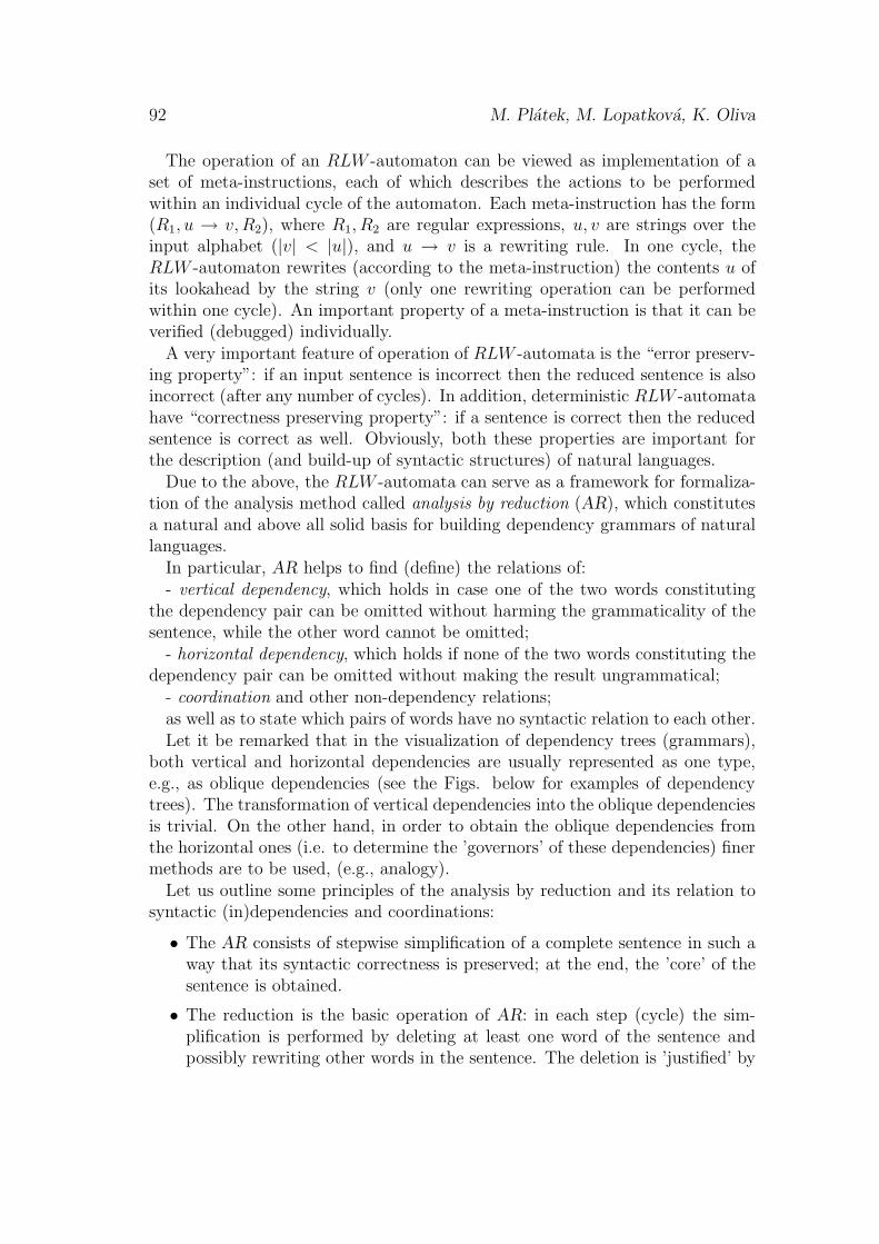
92 M. Platek, M. Lopatkova, K. Oliva
The operation of an RLW -automaton can be viewed as implementation of aset of meta-instructions, each of which describes the actions to be performedwithin an individual cycle of the automaton. Each meta-instruction has the form(R1, u → v, R2), where R1, R2 are regular expressions, u, v are strings over theinput alphabet (|v| < |u|), and u → v is a rewriting rule. In one cycle, theRLW -automaton rewrites (according to the meta-instruction) the contents u ofits lookahead by the string v (only one rewriting operation can be performedwithin one cycle). An important property of a meta-instruction is that it can beverified (debugged) individually.
A very important feature of operation of RLW -automata is the “error preserv-ing property”: if an input sentence is incorrect then the reduced sentence is alsoincorrect (after any number of cycles). In addition, deterministic RLW -automatahave “correctness preserving property”: if a sentence is correct then the reducedsentence is correct as well. Obviously, both these properties are important forthe description (and build-up of syntactic structures) of natural languages.
Due to the above, the RLW -automata can serve as a framework for formaliza-tion of the analysis method called analysis by reduction (AR), which constitutesa natural and above all solid basis for building dependency grammars of naturallanguages.
In particular, AR helps to find (define) the relations of:- vertical dependency, which holds in case one of the two words constituting
the dependency pair can be omitted without harming the grammaticality of thesentence, while the other word cannot be omitted;
- horizontal dependency, which holds if none of the two words constituting thedependency pair can be omitted without making the result ungrammatical;
- coordination and other non-dependency relations;as well as to state which pairs of words have no syntactic relation to each other.Let it be remarked that in the visualization of dependency trees (grammars),
both vertical and horizontal dependencies are usually represented as one type,e.g., as oblique dependencies (see the Figs. below for examples of dependencytrees). The transformation of vertical dependencies into the oblique dependenciesis trivial. On the other hand, in order to obtain the oblique dependencies fromthe horizontal ones (i.e. to determine the ’governors’ of these dependencies) finermethods are to be used, (e.g., analogy).
Let us outline some principles of the analysis by reduction and its relation tosyntactic (in)dependencies and coordinations:
• The AR consists of stepwise simplification of a complete sentence in such away that its syntactic correctness is preserved; at the end, the ’core’ of thesentence is obtained.
• The reduction is the basic operation of AR: in each step (cycle) the sim-plification is performed by deleting at least one word of the sentence andpossibly rewriting other words in the sentence. The deletion is ’justified’ by
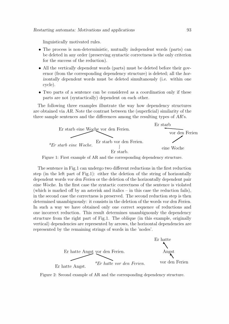
Restarting automata: Motivations and applications 93
linguistically motivated rules.
• The process is non-deterministic, mutually independent words (parts) canbe deleted in any order (preserving syntactic correctness is the only criterionfor the success of the reduction).
• All the vertically dependent words (parts) must be deleted before their gov-ernor (from the corresponding dependency structure) is deleted; all the hor-
izontally dependent words must be deleted simultanously (i.e. within onecycle).
• Two parts of a sentence can be considered as a coordination only if theseparts are not (syntactically) dependent on each other.
The following three examples illustrate the way how dependency structuresare obtained via AR. Note the contrast between the (superficial) similarity of thethree sample sentences and the differences among the resulting types of AR’s.
Er starb vor den Ferien.
Er starb eine Woche vor den Ferien.
*Er starb eine Woche.
Er starb
eine Woche
vor den Ferien
Er starb.
�
3
Figure 1: First example of AR and the corresponding dependency structure.
The sentence in Fig.1 can undergo two different reductions in the first reductionstep (in the left part of Fig.1): either the deletion of the string of horizontallydependent words vor den Ferien or the deletion of the horizontally dependent paireine Woche. In the first case the syntactic correctness of the sentence is violated(which is marked off by an asterisk and italics – in this case the reduction fails),in the second case the correctness is preserved. The second reduction step is thendetermined unambiguously: it consists in the deletion of the words vor den Ferien.In such a way we have obtained only one correct sequence of reductions andone incorrect reduction. This result determines unambiguously the dependencystructure from the right part of Fig.1. The oblique (in this example, originallyvertical) dependencies are represented by arrows, the horizontal dependencies arerepresented by the remaining strings of words in the ’nodes’.
*Er hatte vor den Ferien.
Er hatte Angst vor den Ferien.
Er hatte Angst.
Er hatte
Angst
vor den Ferien
]6
]6
Figure 2: Second example of AR and the corresponding dependency structure.
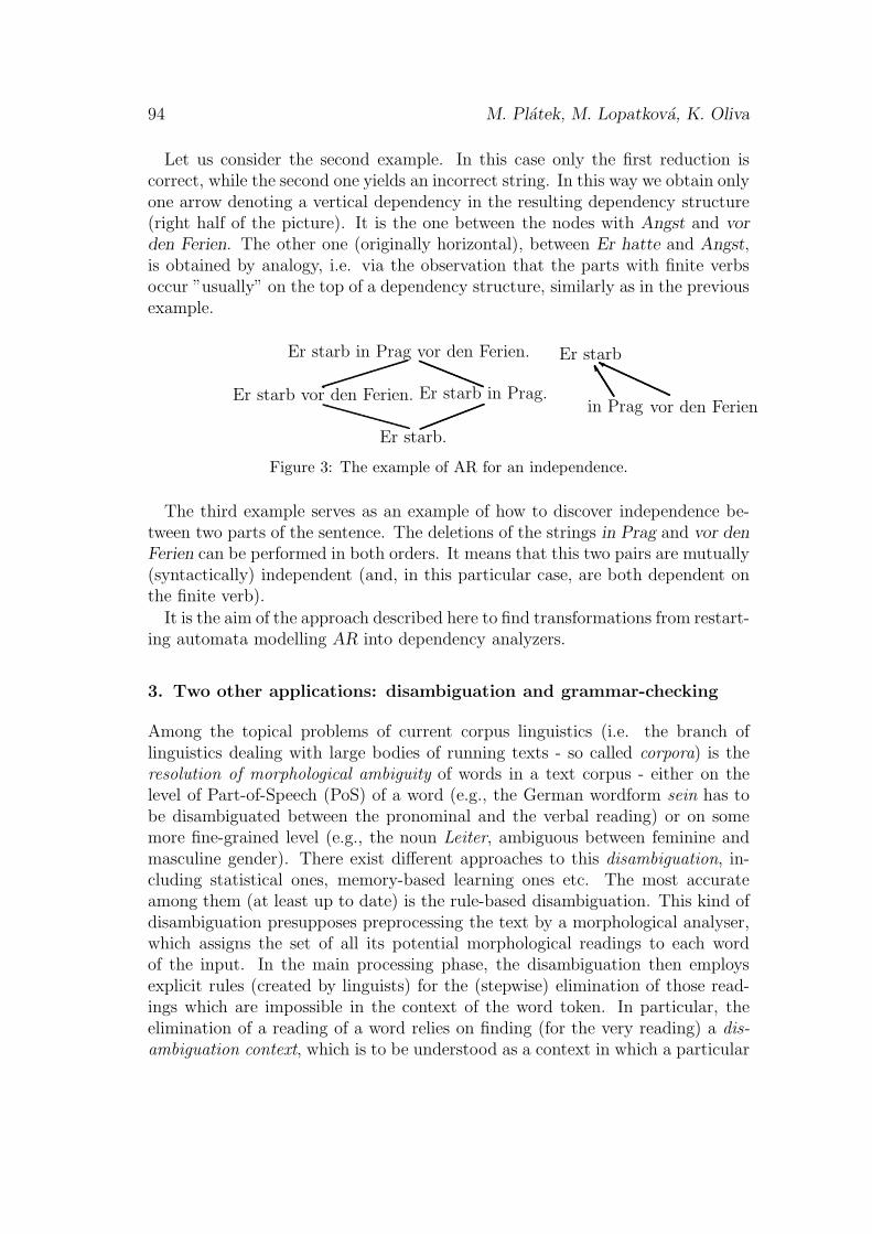
94 M. Platek, M. Lopatkova, K. Oliva
Let us consider the second example. In this case only the first reduction iscorrect, while the second one yields an incorrect string. In this way we obtain onlyone arrow denoting a vertical dependency in the resulting dependency structure(right half of the picture). It is the one between the nodes with Angst and vor
den Ferien. The other one (originally horizontal), between Er hatte and Angst,is obtained by analogy, i.e. via the observation that the parts with finite verbsoccur ”usually” on the top of a dependency structure, similarly as in the previousexample.
Er starb in Prag vor den Ferien.
Er starb vor den Ferien.
Er starb.
Er starb in Prag.
Er starb
in Prag vor den Ferien
]Y
Figure 3: The example of AR for an independence.
The third example serves as an example of how to discover independence be-tween two parts of the sentence. The deletions of the strings in Prag and vor den
Ferien can be performed in both orders. It means that this two pairs are mutually(syntactically) independent (and, in this particular case, are both dependent onthe finite verb).
It is the aim of the approach described here to find transformations from restart-ing automata modelling AR into dependency analyzers.
3. Two other applications: disambiguation and grammar-checking
Among the topical problems of current corpus linguistics (i.e. the branch oflinguistics dealing with large bodies of running texts - so called corpora) is theresolution of morphological ambiguity of words in a text corpus - either on thelevel of Part-of-Speech (PoS) of a word (e.g., the German wordform sein has tobe disambiguated between the pronominal and the verbal reading) or on somemore fine-grained level (e.g., the noun Leiter, ambiguous between feminine andmasculine gender). There exist different approaches to this disambiguation, in-cluding statistical ones, memory-based learning ones etc. The most accurateamong them (at least up to date) is the rule-based disambiguation. This kind ofdisambiguation presupposes preprocessing the text by a morphological analyser,which assigns the set of all its potential morphological readings to each wordof the input. In the main processing phase, the disambiguation then employsexplicit rules (created by linguists) for the (stepwise) elimination of those read-ings which are impossible in the context of the word token. In particular, theelimination of a reading of a word relies on finding (for the very reading) a dis-ambiguation context, which is to be understood as a context in which a particular

Restarting automata: Motivations and applications 95
reading of a particular word is impossible (and hence the reading can be safelyremoved, by means of which disambiguation is performed). Thus, e.g., in theclause weil niemand meinen Eltern einen lebenswurdigen Unterhalt versprechenkonnte the finite verb reading of meinen can be eliminated based on the occur-rence of the unambiguous finite verb konnte and on a rule postulating that inany correct German sentence, a comma or a coordinating conjunction must occursomewhere between two finite verbs (for a complete disambiguation, an applica-tion of another rule, leaning on some other context, would be needed in orderto remove the infinitival reading of meinen). While the creation of such rules isa linguistic-theoretical task, it is quite obvious that their application is an issuewhich is in fact identical to the idea of restarting automata. This can be seenfrom the following two points:
- each rule looks for the configuration it describes (i.e. for a particular readingwith its context), and when such a configuration is detected, the rule servesfor deleting the particular reading (leaving the context untouched); after theapplication of the rule, the whole process has to start again on the newly definedinput (i.e. input after the deletion), using some other rule (or maybe the sameone on another configuration within the sentence)
- successful application of one rule can trigger the application of another rule(the first rule disambiguates and hence gives rise to a context needed for theapplication of the second one); the subtle point here is that this is obviouslydependent not only on the rules, but also on the sentence to be disambiguated:two rules R1 and R2 applied in this order can work well for the sentence S1,while for another sentence S2 this order does not work, but the order R2, R1
would work. This problem has a straightforward and easy solution, however:given a set of rules R1, R2, ..., Rn, this set should be applied such that all possiblerule permutations (non-determinism) are simulated. Thus, any sentence may beprocessed, since also the order needed for this sentence is applied (if all are, thenalso the one needed) - and this is exactly what a non-deterministic restartingautomaton with deletion does.
Let it be mentioned in passing that the approach described above for disam-biguation can also be used for grammar-checking purposes. In particular, if themorphological analysis and the set of disambiguation rules are applied on a sen-tence, and if this results in deleting all readings of one word supplied by themorphological analyser, then it is obvious that the readings of this word are indisaccord with the readings of other words of the sentence, i.e. the sentence issyntactically ill-formed. Thus, the corresponding restarting automaton is in factable to discover (at least some) cases of ill-formed sentences, and in fact alsothe source of the error can be located as the ”last configuration before deletion”(at least in a ”reasonable” number of cases). Some grammar-checking techniquesbased on restarting automata are outlined in [2] and some new techniques of errorrecovery are currently studied.
96 M. Platek, M. Lopatkova, K. Oliva
Acknowledgements
We are indebted to J. Panevova for stimulating discussions concerning analysis byreduction. M. Platek and M. Lopatkova are supported by grants No. 201/02/1456of GACR and LN00A063 of MSMT CR. K. Oliva is supported by Grant No.P16614-G03 of FWF. OeFAI is supported by the Austrian Federal Ministry ofEducation, Science and Culture.
References
[1] P. Jancar, F. Mraz, M. Platek, J. Vogel: On Monotonic Automata with aRestart Operation. J. Autom. Lang. Comb. 4 (1999), 287-311.
[2] V. Kubon, M. Platek: A Grammar Based Approach to Grammar Checkingof Free Word Order Languages, In: Proceedings COLING 94, Vol.II, Kyoto,August, 1994, 906 - 910.
[3] F. Otto: Restarting Automata And Their Relations to the Chomsky hierarchy.In: Z. Esik, Z. Fulop (eds.): Developments in Language Theory, Proceedingsof DLT’2003, LNCS 2710, Springer Verlag, Berlin, 2003, 55 - 74.
[4] K. Oliva, P. Kveton and R. Ondruska: The Computational Complexity ofRule-Based Part-of-Speech Tagging. To appear in: Proceedings of TSD 2003,to be published in the LNAI Series by Springer Verlag.

SOME MORE REGULAR LANGUGAES THAT ARE
CHURCH ROSSER CONGRUENTIAL
Klaus Reinhardt
Institut fur Informatik, University of Tubingene-mail: [email protected]
and
Denis Therien
School of Computer Science, McGill Universitye-mail: [email protected]
ABSTRACT
We show that those languages, where the syntactic monoid is a finite group, areChurch Rosser Congruential Languages (CRCL). We then extend this result to theclass of regular languages whose syntactic monoid lies in the variety DO.
1. Introduction
In [1] McNaughton et al considered finite, length-reducing and confluent string-rewriting systems, which allow to find a unique irreducible shortest representingword for any given word: the Church-Rosser congruential languages (CRCL)are defined as the set of languages, which are the union of finitely many suchequivalence classes. This is defined formally as follows:
A language L ∈ A∗ is in CRCL if there exists a rewriting system R ⊆ {l 7→ r |l, r ∈ A∗, |l| > |r|} allowing derivations
αlβ =⇒R
αrβ with the property that if w∗
=⇒R
w′ and w∗
=⇒R
w′′ then there
is a v ∈ A∗ with w′ ∗=⇒
Rv and w′′ ∗
=⇒R
v and L is the finite union of sets
[we]R = {w | w ∗=⇒
Rwe} for finitely many we.
It is an open problem weather all regular languages are in CRCL.It was shown in [2] that some shuffle languages as well as Level 1 of the
Straubing-Therien hierarchy are in CRCL. Furthermore [2] describes a solutionfor the language (A2)∗ (words of even length on alphabet A = {a, b}), which is
97

98 K. Reinhardt, D. Therien
the smallest nontrivial example for our result since the syntactic monoid for (A2)∗
is the cyclic group Z2.Our approach is as follows: We refine the syntactic monoidM(L) := Σ∗/ ≡L for
the congruence relation ≡L defined by w ≡L v iff ∀u, x ∈ Σ∗ : uwx ∈ L↔ uvx ∈L. The refinement is defined by the construction of a confluent length-reducingstring-rewriting system R ⊂≡L with the property that words exceeding somelength contain an infix l with l 7→ r ∈ R, which leads to a finite ≡R⊇≡L havingthe property that every congruence class has a unique shortest representing word.
For the example (A2)∗ the string-rewriting system R = {aa 7→ λ, bab 7→b, bbb 7→ b} leads to the syntactic monoid consisting of the 10 elements[λ], [ab], [ba], [bb], [abba], [a], [b], [aba], [abb], [bba], where two words are equivalent,if their length, the number of a’s before the first b and the number of a’s afterthe last b differ by an even number and both contain or do not contain a b. Thefirst 5 refine [λ] and the last 5 refine [a] = [b] (two minimal representing stringssince |a| = |b|, which was the reason which made the refinement necessary).
2. The construction for a group
Theorem If the syntactic monoid M(L) is a group, then L ∈ CRCL. Further-more the equivalence relation ≡R⊇≡L is finite but for any length we can chooseR such that all words up to that length are irreducible.
Proof. For L = ∅ or L = {λ} this is trivial, the following is an induction overthe size of the alphabet of L. Let L be a language over the alphabet Σ ={b, a0, ..., as−1}, G = M(L) and n be a multiple of the order of all elementse ∈ G (Note here that n can be chosen arbitrarily large). We use sequences of
consecutive powers of words of the form γi := ban+(i Div s)i Mod s
or in other words γi+sj = ban+ji to build up representing words for each element
in G. For example [a0bba1a2] can be represented as
(ban0 )n−1(ban+1
0 )(ba2n0 )(ba2n+1
1 )(ba3n2 )n−1(ba3n+1
2 ) = γn−10 γsγsnγs(n+1)+1γ
n−1s2n+2γs(2n+1)+2.
Since G is finite, we can find anm such that for every e ∈ G there is a representingword we with [we] = e and bwe = γi0
0 γi11 ...γ
imm . Furthermore since |γ0| + 1 = |γs|,
we can pump i0 and is by some multiples of n for each e in a way such thatl ≤ |we| < l + n for some l chosen big enough.
By induction over the alphabet size we have a confluent, strictly length-reducing rewriting system Ra, which reduces each word w ∈ {a0, ..., as−1}∗ toan irreducible word ww ∈ Irra with [ww] = [w]. Let la := max{|w| | w ∈Irra}.Furthermore we may assume w.l.o.g. that {γ0, ..., γm} ⊆ bIrra (Choosing the n inthe induction large enough). Let
{α1, ...αp} := {w ∈ (bIrra)+ | w primitive and |w| ≤ n or w ∈ bIrra}.
In order to deal with all long cyclic repetitions of these words, we use therewriting-rules Rc = {αl+n
i b 7→ αlib | i ≤ p}. Relevant words not being a part of
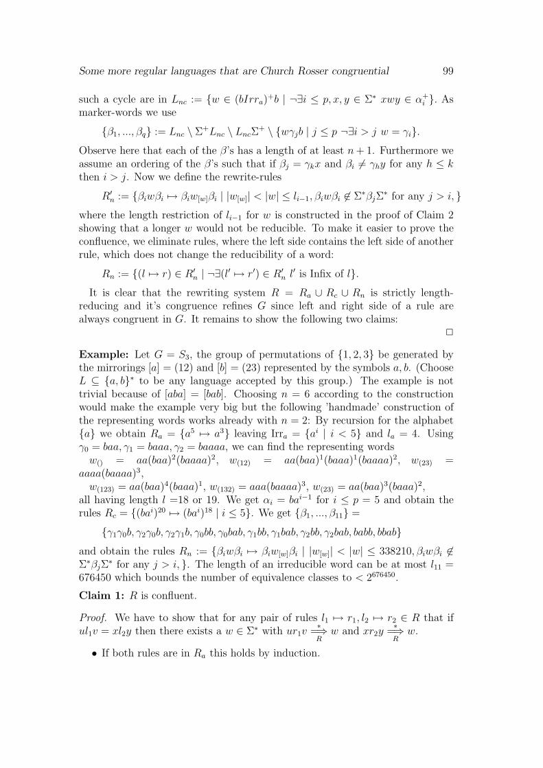
Some more regular languages that are Church Rosser congruential 99
such a cycle are in Lnc := {w ∈ (bIrra)+b | ¬∃i ≤ p, x, y ∈ Σ∗ xwy ∈ α+
i }. Asmarker-words we use
{β1, ..., βq} := Lnc \ Σ+Lnc \ LncΣ+ \ {wγjb | j ≤ p ¬∃i > j w = γi}.
Observe here that each of the β’s has a length of at least n+ 1. Furthermore weassume an ordering of the β’s such that if βj = γkx and βi 6= γhy for any h ≤ kthen i > j. Now we define the rewrite-rules
R′n := {βiwβi 7→ βiw[w]βi | |w[w]| < |w| ≤ li−1, βiwβi 6∈ Σ∗βjΣ
∗ for any j > i, }where the length restriction of li−1 for w is constructed in the proof of Claim 2showing that a longer w would not be reducible. To make it easier to prove theconfluence, we eliminate rules, where the left side contains the left side of anotherrule, which does not change the reducibility of a word:
Rn := {(l 7→ r) ∈ R′n | ¬∃(l′ 7→ r′) ∈ R′
n l′ is Infix of l}.
It is clear that the rewriting system R = Ra ∪ Rc ∪ Rn is strictly length-reducing and it’s congruence refines G since left and right side of a rule arealways congruent in G. It remains to show the following two claims:
2
Example: Let G = S3, the group of permutations of {1, 2, 3} be generated bythe mirrorings [a] = (12) and [b] = (23) represented by the symbols a, b. (ChooseL ⊆ {a, b}∗ to be any language accepted by this group.) The example is nottrivial because of [aba] = [bab]. Choosing n = 6 according to the constructionwould make the example very big but the following ’handmade’ construction ofthe representing words works already with n = 2: By recursion for the alphabet{a} we obtain Ra = {a5 7→ a3} leaving Irra = {ai | i < 5} and la = 4. Usingγ0 = baa, γ1 = baaa, γ2 = baaaa, we can find the representing wordsw() = aa(baa)2(baaaa)2, w(12) = aa(baa)1(baaa)1(baaaa)2, w(23) =
aaaa(baaaa)3,w(123) = aa(baa)4(baaa)1, w(132) = aaa(baaaa)3, w(23) = aa(baa)3(baaa)2,
all having length l =18 or 19. We get αi = bai−1 for i ≤ p = 5 and obtain therules Rc = {(bai)20 7→ (bai)18 | i ≤ 5}. We get {β1, ..., β11} =
{γ1γ0b, γ2γ0b, γ2γ1b, γ0bb, γ0bab, γ1bb, γ1bab, γ2bb, γ2bab, babb, bbab}and obtain the rules Rn := {βiwβi 7→ βiw[w]βi | |w[w]| < |w| ≤ 338210, βiwβi 6∈Σ∗βjΣ
∗ for any j > i, }. The length of an irreducible word can be at most l11 =676450 which bounds the number of equivalence classes to < 2676450.
Claim 1: R is confluent.
Proof. We have to show that for any pair of rules l1 7→ r1, l2 7→ r2 ∈ R that iful1v = xl2y then there exists a w ∈ Σ∗ with ur1v
∗=⇒
Rw and xr2y
∗=⇒
Rw.
• If both rules are in Ra this holds by induction.
100 K. Reinhardt, D. Therien
• If l1 7→ r1 ∈ Ra and l2 7→ r2 ∈ Rc ∪ Rn this holds since l1 ∈ {a0, ..., as−1}∗and l2 ∈ (bIrra)
+b can not overlap.
• If both rules are in Rc this holds since either l1 and l2 overlap only in a smallpart z, which is not changed by the rules, that means w.l.o.g. l1 = αl+n
i1b =
αl+n−1i1
z′z and l2 = αl+ni2b = zz′′αl+n−1
i2and thus w = uαl−1
i1z′zz′′αl−1
i2y or
otherwise αi1 is a rotation of αi2 and thus w = ur1v = xr2y.
• If l1 7→ r1 ∈ Rc and l2 7→ r2 ∈ Rn, again there can be only a short overlappingof the left sides inside a βi, which is not changed since the appearance ofαn+l
k is not allowed in l2 and βi cannot appear in α∗k by definition.
• If both rules are in Rn then either both rules have the same βi in whichcase w = uβiw[z]βiy for ul1v = xl2y = uβizβiy since positions of repeatedoccurances of βi as infix in a word must differ at least n, which garantiesthat w is shorter than ur1v and xr2y or otherwise with different βi1, βi2
with i1 < i2 there is again a short unchanged overlap since in the case thatβi2w
′βi2 ∈ Σ∗βi1Σ∗, we would have βi2w
′βi2 ∈ Σ∗βi1Σ∗βi1Σ
∗, since no βi2
can occur between two βi1’s but then l1 would be an infix of l2, which is notpossible according to the definition of Rn.
2
Claim 2: The number of congruence classes defined by R is finite.
Proof. We show by induction on h that any corresponding to R irreducible wordw, which does not contain any βj with j > h as infix, can only have some boundedlength.
The case h = 0: Assume there would be an arbitrarily long irreducible word.After reading a prefix in Irra, we see the first b, which is the beginning of an infixαi′ . If we continue reading, we can find k < l + n consecutive repetitions of αi′ ,before we find a different αj′, which is not a prefix of a word in αi′Σ
∗. Now thisinfix αk
i′αj′ must have an infix in Lnc and thus a minimal one in Lnc \ Σ+Lnc \LncΣ
+. Therfore the only possibility not to get a β as infix is that αj′ = γj for aj ≤ m and ¬∃i > j αi′ = γi, which can occur at most m times continuing to readthe word. This restricts the length of the word to ≤ l0 = (m+ 1)(l + n)(la + 1).
Step from h − 1 to h: By induction, the length of the prefix before the firstoccurance of of βh and the postfix after the last occurance of βh is bounded bylh. The same holds for the distance between two occurances of βh, but then thereduction-rules for βh ensure that it is even at most l+n and thus this even holdsfor the distance between the first and the last occurance of βh, which means wecan bound the length of the word by lh := 2lh−1 + l + n+ 2(la + 1).
Thus no irreducible word can be longer than lq. 2
Some more regular languages that are Church Rosser congruential 101
3. Extension to DO
The variety DO consists of the closure of group and letter-testing languages underunambiguous concatenation.
Theorem If the syntactic monoid M(L) of a regular language L is in the varietyDO, then L ∈ CRCL.
References
[1] R. McNaughton, P. Narendran, F.Otto. Church-Rosser Thue systems andformal languages. Journal of the ACM, 35:324-344, 1988.
[2] G. Niemann, J. Waldmann. Some regular languages that are Church-Rossercongruential. DLT 2001.
RELATIVISATIONS OF DISJUNCTIVENESS
Cristian S. Calude
Department of Computer Science, The University of AucklandPrivate Bag 92019, Auckland, New Zealand
e-mail: [email protected]
and
Ludwig Staiger
Martin-Luther-Universitat Halle-Wittenberg, Institut fur Informatik,von-Seckendorff-Platz 1, D - 06099 Halle, Germany
e-mail: [email protected]
ABSTRACT
The present paper proposes a generalisation of the notion of disjunctive (or rich)sequence, that is, of an infinite sequence of letters having each finite sequence as asubword.
Our aim is to give a reasonable notion of disjunctiveness relative to a given setof sequences F . We show that a definition like “every subword which can occur
infinitely often in F has to occur infinitely often in the sequence” fulfils propertiessimilar to the original unrelativised notion of disjunctiveness.
Finally, we investigate our concept of generalised disjunctiveness in spaces ofCantor expansions of reals.
Keywords: Disjunctive sequences, Cantor expansion, density, porosity.
A semi-infinite sequence is called disjunctive (or rich) if it has all finite wordsas subwords (infixes) (cf [8, 9]). This condition is, obviously, equivalent to havingevery finite word infinitely often as infix.
In connection with disjunctive sequences ξ over {0, . . . , r−1} their real counter-parts 0.ξ were considered. It is interesting to note that in contrast to propertieslike randomness or Kolmogorov complexity (cf. [1, 2, 7, 17]) disjunctiveness is notinvariant under base conversion, more precisely speaking, if ξ ∈ {0, . . . , r − 1}ω
and η ∈ {0, . . . , b − 1}ω satisfy 0.ξ = 0.η (as reals) then ξ might be disjunctivewhereas η need not be so. For a more detailed treatment see [6].
Along with the usual base r expansions of real numbers one can also considerso-called Cantor expansions. In general, a Cantor expansion of a real is an element
102

Relativisations of disjunctiveness 103
ξ ∈ X(f) where X(f) is a certain subset of the Baire space INω where the set ofallowed letters at position i (i ≥ 1) is specified as {0, . . . , f(i) − 1} (cf. [4, 5]):Let f(1), f(2), . . . , f(n), . . . be a fixed infinite sequence of positive integers greaterthan 1. Using a point we form the sequence 0.x1x2 . . . xi . . . such that xn ∈ IN, 0 ≤xn < f(n), for all n ≥ 1. The real number
α :=n∑
i=1
xi
f(1) · f(2) · · ·f(i)
has 0.x1x2 . . . as (one of) its Cantor expansion(s).It is easy to see that the set of subwords occurring in a sequence ξ ∈ X(f) :=
{x1x2 . . . xi . . . : 0 ≤ xi < f(i)} depends on the function f : IN → IN, and, more-over, some subword occurring once in some ξ ∈ X(f) might not occur infinitelyoften in any η ∈ X(f).
Thus the definition of disjunctiveness for Cantor expansions needs some gen-eralisation. In this paper we propose a possible modification of the notion ofdisjunctive sequence in the following way1: A sequence ξ ∈ F ⊆ INω is F -
disjunctive if and only if every infix which may occur infinitely often in some
sequence η ∈ F occurs infinitely often in ξ. Here, of course, the phrase “whichmay occur infinitely often in some sequence” needs further specification.
1. Preliminaries
1.1. Notation
By IN = {0, 1, 2, . . .} we denote the set of natural numbers. In order to treatarbitrary finite alphabets we let Xr := {0, . . . , r−1} be an alphabet of cardinality|Xr| = r, r ∈ IN, r ≥ 2. In this paper we will use finite alphabets Xr, r ∈ IN,and IN as a countably infinite alphabet. By X∗ we denote the set of finite strings(words) over the alphabet X, including the empty word e. We consider also thespace Xω of infinite sequences (ω-words) over X. For w ∈ X∗ and η ∈ X∗ ∪Xω
let w ·η be their concatenation. This concatenation product extends in an obviousway to subsets W ⊆ X∗ and B ⊆ X∗ ∪Xω.
By “⊑” we denote the prefix relation, and pref(B) :=⋃
η∈B pref(B) are thelanguages of finite prefixes of η and B, respectively. The set of subwords (infixes)of η ∈ X∗ ∪Xω will be denoted by infix(η) := {w : w ∈ X∗ ∧ ∃v(vw ⊑ η)}.
In the sequel, we shall confine ourselves to sets of the form X(f) ⊆ IN as definedin the introduction.2 Introducing a metric in X(f) as follows
ρf(ξ, η) := inf{ |w|∏
i=1
f(i)−1 : w < ξ ∧ w < η}
(1.1)
1We base our generalisation on infinite occurrences of subwords. This proposal seems to bejustified by the results of Section 2.
2For f ≡ r this covers also the case X(f) = Xωr .
104 C.S. Calude, L. Staiger
we make (X(f), ρf) a compact metric space. It is easily verified that ρf is indeeda metric which, in addition, satisfies the ultra-metric inequality.
ρf(ζ, ξ) ≤ max {ρf (ζ, η), ρf(ξ, η)} (1.2)
Open (in view of Eq. (1.2) they are simultaneously closed) balls in this space(X(f), ρf) are the sets X(f) ∩ w · INω. Then open sets in X(f) are of the formX(f)∩W ·INω where W ⊆ pref(X(f)). From this it follows that a subset F ⊆ X(f)
is closed if and only if pref(ξ) ⊆ pref(F ) implies ξ ∈ F .The closure of a subset F ⊆ X(f) in the space (X(f), ρf), that is, the smallest
closed subset of Xω containing F is denoted by C(F ). One has C(F ) = {ξ :pref(ξ) ⊆ pref(F )}.
It should be mentioned that, due to the special choice of the metric (seeEq. (1.1)), the following uniformity property for balls is satisfied.
∑
x∈Xf(|w|)+1
diamf(X(f) ∩ w · x · INω) = diamf (X
(f) ∩ w · INω) (1.3)
1.2. Density, Baire Category and Porosity
Next, we introduce the concept of topological density, Baire category and porosityfor our complete metric space (X(f), ρf ). (see e.g. [10, 11, 18])
A subset M ⊆ X(f) is called dense in X(f) provided its closure C(F ) is thewhole space X(f). A set M ⊆ X(f) is nowhere dense in (X(f), ρf ) provided itsclosure C(M) does not contain a nonempty open subset.
A set F is of first Baire category iff it is a countable union of nowhere densesets, otherwise it is of second Baire category. The complements of sets of firstBaire category are called residual.
The concept of porous subsets in general metric spaces is introduced e.g. in[18, Section 2.C]. We explain it for the space (X(f), ρf).
Let λ(E, u) := sup{diamf (w · INω ∩X(f)) : u ⊑ w ∧ w · INω ∩ E = ∅} be thediameter of a largest ball contained u · INω ∩X(f) but disjoint to E, and
p(E, ξ) := lim supu→ξ
λ(E, u)
diamf(u · INω ∩X(f))(1.4)
is the porosity of E at the point ξ. A set E ⊆ X(f) is called porous if p(E, ξ) > 0for all ξ ∈ X(f), and a set F ⊆ X(f) is called σ-porous iff it is a countable unionof porous sets. It is obvious that every porous set is nowhere dense, but theconverse need not be true (see [18]). It should be noted, however, that in (Xω
r , ρ)every nowhere dense set definable by a finite automaton is porous ([12, 15, 16]).
1.3. Disjunctive sequences in Xωr
Finally, we list some properties of the set of disjunctive sequences Dr ⊆ Xωr
known from [3, 16]
Relativisations of disjunctiveness 105
Theorem 1 1. Dr is a residual set in Xωr .
2. Xωr \Dr =
⋃
w∈X∗r
(
Xωr \X∗
r · w ·Xωr
)
=⋃
w∈X∗r
(X |w|r \ {w})ω
3. Xωr \Dr is the union of all nowhere dense ω-languages definable by a finite
automaton.
4. Xωr \Dr is σ-porous.
5. µ(Dr) = 1 for all non-degenerate product measures on Xωr .
2. Generalised Disjunctiveness
In this section we make precise what we mean when we say informally that anω-word ξ ∈ F should be called disjunctive if and only if every word w ∈ IN∗ whichcan appear infinitely often as an infix in F has to appear infinitely often as aninfix of ξ. To this end we observe that a necessary condition when a word w canappear infinitely often as an infix in F is the following one.
Let Infix∞(F ) := {w : ∃∞n∃u(|u| = n∧uw ∈ pref(F )}. An ω-word ξ is calledF -disjunctive provided ξ ∈ F and Infix∞(F ) = Infix∞(ξ) .
For general subsets of INω or X(f) this condition is still complicated to treat. Tothis end we introduce the following notion which, when satisfied for Infix∞(F ),will alleviate the investigation of disjunctive sequences. A set W ⊆ IN∗ is referredto as left prolongable if and only if for every w ∈ W there is a x ∈ IN such thatx · w ∈ W .
Proposition 2 Let Infix∞(F ) be left prolongable. Then infix(ξ) ⊇ Infix∞(F )implies Infix∞(ξ) ⊇ Infix∞(F ) for all ξ ∈ F .
The following example shows that prolongability is essential.
Example 1 Let F :=∏∞
i=2{i1, 00}. Then Infix∞(F ) = 0∗ ∪ 1 · 0∗, and, indeed,for η = 210ω we have infix(η) ⊇ Infix∞(F ) ⊃ Infix∞(η) = 0∗.
As a corollary to Proposition 2 we obtain properties of the set of all F -disjunctiveω-words similar to Property 2 in Theorem 1 for Dr.
Corollary 3 If Infix∞(F ) is left prolongable, thenDF =
⋂
w∈Infix∞(F )(F ∩ IN∗ · w · INω) is the set of all F -disjunctive ω-words,
and
F\DF =⋃
w∈Infix∞(F )(F \ IN∗ · w · INω) =
⋃
w∈Infix∞(F )
(
F∩|w|−1⋂
j=0
INj·(IN|w|\{w})ω
)
.
106 C.S. Calude, L. Staiger
3. Disjunctiveness in ultimately connected sets
Here we consider the case of a subset F of a Cantor space Xωr having the following
property.
∀u(u ∈ pref(F ) → ∃v(v ∈ X∗r ∧ u · v · F ⊆ F )) (3.5)
Those sets were called ultimately connected and can be characterised by the so-called stabiliser of F ⊆ Xω
r , Stab(F ) (cf. [13, 14]).
Stab(F ) := {w : w ∈ pref(E) \ {e} ∧ w · F ⊆ F} (3.6)
Stab(F ) is closed under concatenation, that is, is a subsemigroup of X∗r .
Proposition 4 An ω-language F ⊆ Xωr is ultimately connected if and only if
pref(F ) ⊆ pref(Stab(F ))
Examples of ultimately connected ω-languages are the so-called ω-power lan-guages W ω := {∏∞
i=1wi : wi ∈ W \ {e}}. Obviously, the stabiliser of an ω-powerlanguage W ω satisfies W ∗ \ {e} ⊆ Stab(W ω) ⊆ Stab(C(W ω)) ⊆ pref(W ω) andStab(W ω) ·W ω = W ω.
For ultimately connected ω-languages F the language Infix∞(F ) has the fol-lowing properties.
Proposition 5 Infix∞(F ) = infix(Stab(F )) and Infix∞(F ) is two-sided pro-longable.
Corollary 3 applies immediately to ultimately connected ω-languages.
Corollary 6 If F ⊆ Xωr is ultimately connected then
F \DF =⋃
w∈Stab(F )(F \X∗
r · w ·Xωr ) =
⋃
w∈Stab(F )
(
F ∩|w|−1⋂
j=0
Xjr ·(X |w|
r \{w})ω
)
.
We conclude the part on ultimately connected ω-languages by mentioning someresults from [14] similar to Theorem 1.3 concerning ω-languages definable by afinite automaton which are nowhere dense in F . To this end we mention thata set E ⊆ Xω
r is nowhere dense in F ⊆ Xωr if and only if ∀u(u ∈ pref(F ) →
∃v (v ∈ X∗r ∧ u · v ∈ pref(F ) \ pref(E))).
Lemma 7 If F ⊆ Xωr is ultimately connected and E is definable by a finite
automaton then
1. E is nowhere dense in F iff ∃w(w ∈ Stab(F )∧E ∩C(F ) ⊆ C(F )\Stab(F )∗ ·w ·Xω
r ), and
2. E is nowhere dense in F iff ∃w(w ∈ Stab(F ) ∧ E ⊆ C(F ) \ X∗r · w · Xω
r )provided E ⊆ C(F ).
Relativisations of disjunctiveness 107
4. Disjunctiveness for Cantor expansions
In this section we derive some simple properties of the set Infix∞(X(f)). Fromthese properties, in particular, we derive that Infix∞(X(f)) is left prolongable,whence properties like Proposition 2 and Corollary 3 hold for the set of all dis-junctive ω-words in X(f), Df , independently of the choice of f .
We start with a simple property.
Proposition 8 1. u · INω ⊆ IN∗ · w · INω iff w ∈ infix(u).
2. Let u ∈ pref(X(f)) and |u| ≤ n.Then 0n · w ∈ pref(X(f)) iff u · 0n−|u| · w ∈ pref(X(f)).
3. If w ∈ Infix∞(X(f)) then {0, 1}∗ · w · {0, 1}∗ ⊆ Infix∞(X(f)).
Lemma 9 Let κf(n) := lim supi→∞ min{f(i+ j) : 1 ≤ j ≤ n} ≥ r.Then {0, 1}∗ ·Xn
r · {0, 1}∗ ⊆ Infix∞(X(f)).
As an immediate consequence of Proposition 8.3 we obtain the announced prop-erty.
Corollary 10 Infix∞(X(f)) is left prolongable, for every function f : IN → IN \{0, 1}.
5. Topological Properties of X(f) \ IN∗ · w · INω
In this section we are going to investigate some topological properties of the setof disjunctive sequences in X(f). First we investigate the relationship to densityand measure. We start with a simple proposition which holds for all functionsf : IN → IN \ {0, 1}.
Lemma 11 The set X(f) \ IN∗ · w · INω is nowhere dense in (X(f), ρf ) wheneverw ∈ Infix∞(X(f)).
In contrast to Theorem 1.5 the measure property does not hold in general.
Example 2 Let µ be the measure on X(f) induced by the Lebesgue measure on[0, 1]. For the function f(i) := (i + 1)2 and the set F := X(f) \ IN∗ · 0 · INω =∏∞
i=1(Xf(i) \ {0}) we have µ(F ) =∏∞
i=1(1 − f(i)−1) =
∏∞
j=2(1 − j−2) > 0 .
From [18] it is known that a porous set F ⊆ X(f) is nowhere dense and hasmeasure µ(F ) = 0. As we have seen in Example 2 the complement of the setof disjunctive sequences in X(f) may have positive measure. Next we investigatehow this behaviour depends on the function f .
A first result and a comparison with Theorem 1 show that the case of boundedfunctions is similar to the case of constant alphabets.

108 C.S. Calude, L. Staiger
Lemma 12 If f : IN → IN is bounded then for every w ∈ Infix∞(X(f)) the setX(f) \ IN∗ · w · INω is porous in X(f).
Thus the case when f is unbounded needs special treatment. We obtain thefollowing sufficient condition for the non-porosity of sets X(f) \ IN∗ · w · INω.
Theorem 13 If f : IN → IN is unbounded and kf := sup{k :f−1(k) is infinite} < ∞ then for every i > kf and v ∈ {0, 1}∗ the setX(f) \ IN∗ · vi · INω is not porous in X(f).
We may, however, have also sets of the form X(f) \ IN∗ ·w · INω which are porous.
Example 3 Define
f(i) :=
n, if i = n2 for some n ∈ IN, and
2 , otherwise.
Then the set X(f) \ IN∗ · w · INω is porous in X(f) whenever w ∈ {0, 1}∗.
In particular, the condition of Theorem 13 is satisfied when f tends to infinity.
Corollary 14 If limn→∞ f(n) = ∞ then Infix∞(X(f)) = IN∗ and each set X(f) \IN∗ · w · INω is not porous in X(f).
References
[1] J.-Y. Cai, J. Hartmanis: On Hausdorff and Topological Dimensions ofthe Kolmogorov Complexity of the Real Line. J. Comput. System Sci. 49(1994) 3, 605–619.
[2] C.S. Calude, H. Jurgensen: Randomness as an Invariant for NumberRepresentations. In: Results and Trends in Theoretical Computer Science(H. Maurer, J. Karhumaki, G. Rozenberg Eds.), Lecture Notes inComput. Sci. 812, Springer-Verlag, Berlin 1994, 44–66.
[3] C.S. Calude, L. Priese, L. Staiger: Disjunctive Sequences: AnOverview. CDMTCS Research Report 063, Auckland (1997)
[4] S. Drobot: Real Numbers. Prentice-Hall, Englewood Cliffs, New Jersey,1964.
[5] G. H. Hardy, E. M. Wright: An Introduction to the Theory of Num-bers. Cambridge Univ. Press, London 1954.
[6] P. Hertling: Disjunctive ω-words and Real Numbers. J.UCS (Journal ofUniversal Computer Science) 2 (1996), 549 – 568.
[7] P. Hertling, K. Weihrauch: Random Elements in Effective Topologi-cal Spaces with Measure. Inform. and Comput. 181 (2003), 32–56.
Relativisations of disjunctiveness 109
[8] H. Jurgensen, H.J. Shyr, G. Thierrin: Disjunctive ω-languages. Elek-tron. Informationsverarb. Kybernetik EIK 19 (1983), 267–278.
[9] H. Jurgensen, G. Thierrin: On ω-languages whose Syntactic Monoidis Trivial. Intern. J. Comput. Inform Sci. 12 (1983), 359 -365.
[10] K. Kuratowski: Topology I. Academic Press, New York 1966.
[11] J.C. Oxtoby: Measure and Category. Springer-Verlag, Berlin 1971.
[12] L. Staiger: Regulare Nullmengen. Elektron. Informationsverarb. Kyber-netik EIK 12 (1976), 307–311.
[13] L. Staiger, A note on connected ω-languages. Elektron. Informationsverarb.Kybernetik EIK 16 (1980), 245–251.
[14] L. Staiger, On ω-power languages, In: New Trends in Formal Languages,Control, Cooperation, and Combinatorics, (Gh. Paun and A. Salomaa
Eds.), Lecture Notes in Comput. Sci. No. 1218, Springer–Verlag, Berlin.377–393.
[15] L. Staiger: Rich ω-words and Monadic Second-order Arithmetic. In:Computer Science Logic, 11th International Workshop, CSL’97, SelectedPapers (M. Nielsen and W. Thomas Eds.), Lecture Notes in Comput.Sci. 1414, Springer-Verlag, Berlin (1998), 478–490.
[16] L. Staiger: How Large is the Set of Disjunctive Sequences? J.UCS (Jour-nal of Universal Computer Science) 8 (2002), 348–362.
[17] L. Staiger: The Kolmogorov Complexity of Real Numbers. Theoret. Com-put. Sci. 284 (2002), 455 – 466.
[18] L. Zajıcek: Porosity and σ-porosity. Real Analysis Exch. 13 (1987-88),314–350.
ON THE SIZE OF HYBRID NETWORKS OF
EVOLUTIONARY PROCESSORS
Ralf Stiebe
Fakultat fur Informatik, Otto-von-Guericke-Universitat MagdeburgPF 4120, D-39016 Magdeburg, Germany
e-mail: [email protected]
ABSTRACT
We show that any recursively enumerable language can be generated by a hybridnetwork of evolutionary processors (HNEP) of constant size. Moreover, we showthat HNEPs of size 2 can generate non-context-free languages.
Keywords: Evolutionary processors, descriptional complexity.
In a series of papers, Mitrana and others introduced networks of evolutionaryprocessors and variants [1, 2, 3, 4]. Anevolutionary processor contains a set ofstrings and can perform the following elementary operations (evolution steps):insert a symbol, delete a symbol, replace a symbol by another symbol. Moreover,it can be required that insertions and deletions can only take place on the leftor right end. In a hybrid network of evolutionary processors (HNEP), a set ofprocessors is connected according to an underlying graph. Moreover, the pro-cessors have input and output filters (permitting and forbidding random contextconditions). In a communication step, any string matching the output conditionleaves a processor and enters a neighboring processor if it passes the input filter.A computation of an HNEP consists of an alternating sequence of evolutionaryand communication steps. The generated language is the set of all strings thatreach a specified output processor.
It is shown in [2] that any recursively enumerable language L ⊆ V ∗ can begenerated by an HNEP with 26 + 3|V | processors. Moreover, it is proved thatany HNEP with 1 processor generates a regular language and that there is anon-context-free language generated by an HNEP with 4 processors. We improvethese results as follows:
Theorem 1 There is a fixed graph G such that any recursively enumerable lan-guage L is generated by an HNEP with underlying graph G.
110
On the size of hybrid networks of evolutionary processors 111
Theorem 2 There is an HNEP with 2 processors that generates a non-context-free language.
References
[1] Juan Castellanos, Carlos Martın-Vide, Victor Mitrana, and Jose Sempere.Networks of evolutionary processors. Acta Informatica, 39:517–529, 2003.
[2] Erzsebet Csuhaj-Varju, Carlos Martın-Vide, and Victor Mitrana. Hybridnetworks of evolutionary processors are computationally complete. Submitted,2003.
[3] Carlos Martın-Vide, Victor Mitrana, Mario Perez-Jimenez, and FernandoSancho-Caparrini. Hybrid networks of evolutionary processors. In Geneticand Evolutionary Computation - GECCO 2003, LNCS, pages 401–412, 2003.
[4] Victor Mitrana. Some complexity aspects of hybrid networks of evolutionaryprocessors. In Proceedings of DCFS 2003, pages 53–65, 2003.
GI-Fachgruppe 0.1.5
”Automaten und Formale
Sprachen“
Wahl der Fachruppenleitung
Die Wahl der Leitung der GI-Fachgruppe 0.1.5 wurde am 1. Oktober 2003 im Rah-men der Fachgruppen-Sitzung auf dem 13. Theorietag
”Automaten und Formale
Sprachen“ in Herrsching durchgefuhrt. Anwesend waren folgende Fachgruppen-Mitglieder:
Suna Bensch (Potsdam), Henning Bordihn (Potsdam), Jurgen Dassow (Magde-burg), Henning Fernau (Tubingen), Rudolf Freund (Wien), Jens Glockler (Gie-ßen), Maia Hoeberechts (London, Ontario), Markus Holzer (Munchen), EkkartKindler (Paderborn), Daniel Kirsten (Paris), Andreas Klein (Kassel), Martin Ku-trib (Gießen), Martin Lange (Munchen), Martin Leucker (Uppsala), AndreasMalcher (Frankfurt), Frantisek Mraz (Prag), Marion Oswald (Wien), FriedrichOtto (Kassel), Martin Platek (Prag), Bernd Reichel (Magdeburg), Jens Reimann(Gießen), Klaus Reinhardt (Tubingen), Ludwig Staiger (Halle) und Ralf Stiebe(Magdeburg).
Zum Wahlleiter wurde Henning Fernau bestimmt. Der Wahlleiter stellte die 6Kandidaten vor. Von den 24 abgegebenen Stimmen waren 24 gultig. Es wurdengewahlt
Henning Bordihn (Potsdam), Jurgen Dassow (Magdeburg), Markus Holzer (Mun-chen), Martin Kutrib (Gießen) und Friedrich Otto (Kassel).
Alle Gewahlten nahmen die Wahl an. Das Wahlprotokoll wurde verlesen undgenehmigt.
113
Wahl des Fachgruppensprechers
Am 1. Oktober 2003 einigten sich die anwesenden Mitglieder der Fachgruppen-leitung darauf, daß Herr Otto das Amt des Sprechers und Herr Kutrib das Amtdes stellvertretenden Sprechers wahrnehmen werden. Dieser Vorschlag wurde ein-stimmig angenommen. Herr Dassow und Herr Kutrib nahmen die Wahl an.
114

TeilnehmerInnenliste
• Suna BenschInstitut fur InformatikUniversitat PotsdamAugust-Bebel-Straße 8914482 Potsdam
Tel.: +49-331-977-3028Fax: +49-331-977-3022
e-mail: [email protected]
• Eike BestDepartment fur InformatikUniversitat OldenburgFakultat II26111 Oldenburg
Tel.: +49-441-798-2973Fax: +49-441-798-2965
e-mail: [email protected]
• Henning BordihnInstitut fur InformatikUniversitat PotsdamAugust-Bebel-Straße 8914482 Potsdam
Tel.: +49-331-977-3027Fax: +49-331-977-3022
e-mail: [email protected]
• Jurgen DassowFakultat fur Informatik
115

TeilnehmerInnenliste 116
Otto-von-Guericke-Universitat MagdeburgPostfach 412039016 Magdeburg
Tel.: +49-391-67-18853Fax: +49-391-67-12018
e-mail: [email protected]
• Javier EsparzaInstitut fur Formale Methoden der InformatikUniversitat StuttgartUniversitatsstr. 3870569 Stuttgart
Tel.: +49-711-7816-455Fax: +49-711-7816-370
e-mail: [email protected]
• Henning FernauSchool of Electrical Engineering and Computer ScienceUniversity of NewcastleUniversity DriveCallaghan, NSW 2308Australia
Tel.: +61-2-4921-6076Fax: +61-2-4921-6929
e-mail: [email protected]
• Rudolf FreundInstitut fur ComputersprachenTechnische Universitat WienFavoritenstr. 9A-1040 WienOsterreich
Tel.: +43-1-58801-18542Fax: +43-1-58801-18599
e-mail: [email protected]
TeilnehmerInnenliste 117
• Jens GlocklerInstitut fur InformatikUniversitat GießenArndtstr. 235392 Gießen
Tel.: +49-641-99-32142Fax: +49-641-99-32149
e-mail: [email protected]
• Maia HoeberechtsDepartment of Computer ScienceUniversity of Western OntarioN6A 5B7 LondonOntario, Canada
Tel.:Fax:
e-mail: [email protected]
• Markus HolzerInstitut fur InformatikTechnische Universitat MunchenBoltzmannstraße 385748 Garching bei Munchen
Tel.: +49-89-289-17230Fax: +49-89-289-17207
e-mail: [email protected]
• Roman KonigInstitut fur Informatik IIIUniversitat Erlangen-NurnbergMartensstraße 391058 Erlangen
Tel.: +49-9131-8527921Fax: +49-9131-39388
e-mail: [email protected]
TeilnehmerInnenliste 118
• Ekkart KindlerInstitut fur InformatikUniversitat Paderborn33098 Paderborn
Tel.: +49-5251-60-3320Fax: +49-5251-60-3530
e-mail: [email protected]
• Daniel KirstenLIAFAUniversite Denis Diderot – Case 70142, place JussieuF-75251 Paris Cedex 05France
Tel.:Fax: +33-1-44276849
e-mail: [email protected]
• Andreas KleinFachbereich fur Mathematik und InformatikUniversitat KasselHeinrich-Plett-Straße 4034132 Kassel
Tel.: +49-561-804-4367Fax:
e-mail: [email protected]
• Martin KutribInstitut fur InformatikUniversitat GießenArndtstr. 235392 Gießen
Tel.: +49-641-99-32144Fax: +49-641-99-32149
e-mail: [email protected]
TeilnehmerInnenliste 119
• Martin LangeLFE Theoretische InformatikInstitut fur InformatikLudwig-Maximilians-UniversitatOettingenstr. 6780538 Munchen
Tel.: +49-89-2180 9313Fax: +49-89-2180 9338
e-mail: [email protected]
• Martin LeuckerDepartment of Computer ScienceUppsala UniversityBox 337SE-75105 UppsalaSweden
Tel.: +46-18-471-5779Fax:
e-mail: [email protected]
• Andreas MalcherFB InformatikJohann Wolfgang Goethe-UniversitatPostfach 11 19 3260054 Frankfurt am Main
Tel.: +49-69-798-28413Fax: +49-69-798-28334
e-mail: [email protected]
• Frantisek MrazDepartment of Computer ScienceCharles UniversityMalostranske nam. 25CZ-118 00 Praha 1Czech Republic
Tel.: +42-2-21914219Fax: +42-2-21914281
TeilnehmerInnenliste 120
e-mail: [email protected]
• Marion OswaldInstitut fur ComputersprachenTechnische Universitat WienFavoritenstr. 9A-1040 WienOsterreich
Tel.:Fax:
e-mail: [email protected]
• Friedrich OttoArbeitsgruppe Theoretische InformatikFachbereich Mathematik/InformatikUniversitat Gesamthochschule KasselHeinrich-Plett-Straße 4034132 Kassel
Tel.: +49-561-804-4573Fax: +49-561-804-4008
e-mail: [email protected]
• Martin PlatekKTIML MFFCharles UniversityMalostranske nam. 25CZ-118 00 Praha 1Czech Republic
Tel.:Fax:
e-mail: [email protected]
• Bernd ReichelFakultat fur InformatikOtto-von-Guericke-Universitat MagdeburgPostfach 412039016 Magdeburg
TeilnehmerInnenliste 121
Tel.: +49-391-67-12851Fax: +49-391-67-11250
e-mail: [email protected]
• Jens ReimannInstitut fur InformatikUniversitat GießenArndtstr. 235392 Gießen
Tel.: +49-641-99-32153Fax: +49-641-99-32149
e-mail: [email protected]
• Klaus ReinhardtWilhelm-Schickard Institut fur InformatikUniversitat TubingenSand 1372076 Tubingen
Tel.: +49-7071-29-77566Fax: +49-7071-29-5061
e-mail: [email protected]
• Karsten SchmidtInstitut fur InformatikHumboldt-Universitat zu BerlinUnter den Linden 610099 Berlin
Tel.: +49-30-2093-3083Fax:
e-mail: [email protected]
• Ludwig StaigerInstitut fur InformatikMartin-Luther-Universtitat Halle-WittenbergVon-Seckendorff-Platz 106099 Halle an der Saale
TeilnehmerInnenliste 122
Tel.: +49-345-5524714Fax: +49-345-5527009
e-mail: [email protected]
• Ralf StiebeFakultat fur InformatikOtto-von-Guericke-Universitat MagdeburgPostfach 412039016 Magdeburg
Tel.: +49-391-67-12457Fax: +49-391-67-12018
e-mail: [email protected]
• Bettina SunckelInstitut fur InformatikJohann Wolfgang Goethe-UniversitatPostfach 11 19 3260054 Frankfurt am Main
Tel.: +49- 69-7982 8419Fax: +49-69-7982 8334
e-mail: [email protected]


