Technische Universit¨ at Braunschweig Embedding Force Control in a Robot Control System TorstenKr¨oger Studienarbeit Betreuer: Dipl.-Ing. Bernd Finkemeyer 18. M¨ arz 2002 Institut f¨ ur elektrische Messtechnik und Grundlagen der Elektrotechnik Prof. Dr.-Ing. J.-Uwe Varchmin
Transcript
Technische Universitat Braunschweig
Embedding Force Control in a Robot Control System
Torsten Kroger
Studienarbeit
Betreuer: Dipl.-Ing. Bernd Finkemeyer
18. Marz 2002
Institut fur elektrische Messtechnik und
Grundlagen der Elektrotechnik
Prof. Dr.-Ing. J.-Uwe Varchmin
Erklarung
Hiermit erklare ich, dass die vorliegende Arbeit selbstandig nur unter Verwendung deraufgefuhrten Hilfsmittel von mir erstellt wurde.
Braunschweig, den 18. Marz 2002
Unterschrift
Kurzfassung
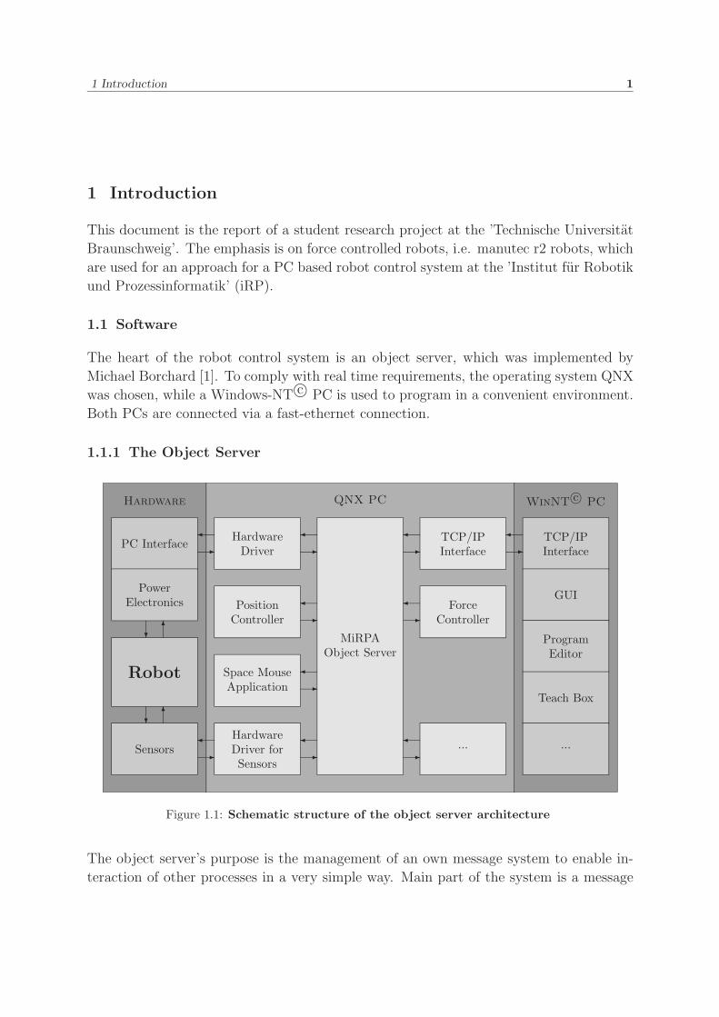
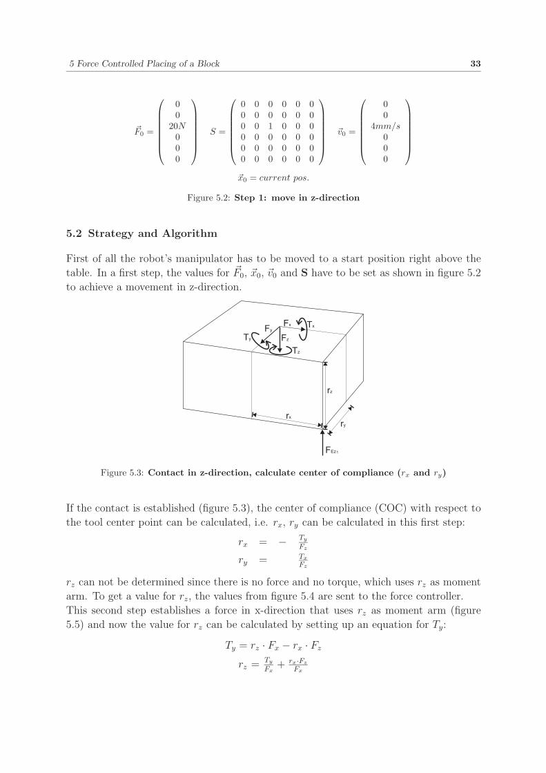
Das vorliegende Manuskript ist die Dokumentation einer Studienarbeit an der Techni-schen Universitat Braunschweig. Zielsetzung ist es, einen Kraftregler in einer vorhandenenRobotersteuerung zu implementieren. Diese Steuerung, der Treiber fur einen Kraft-/Momentensensor sowie der Treiber einer Space Mouse werden einleitend beschrieben.Nach der Vorstellung moglicher Kraftregelkonzepte folgt die Beschreibung des implemen-tierten Reglers, und abschließend wird eine Anwendung des Reglers dokumentiert, dessenZiel das kraftgeregelte Absetzen eines windschiefen Klotzes auf eine Ablage ist.
Abstract
This document is the report of a student research project at the ’Technische UniversitatBraunschweig’. Its aim is to embed a force controller into an existing robot control ar-chitecture. Introductory, this architecture, the driver for a force-torque sensor as wellthe driver for a Space Mouse are described. After the presentation of several force con-trol approaches, the implemented force controller is detailed. An application, the forcecontrolled placing a warped block, is documented finally.
Acknowledgements
During this student research project, I have interacted with many people. Each hashad some influence on the final version of this document. I greatly appreciate all thehelpful chats with Niels Otten during the time in the robot laboratory. My roommate,Christian Meiners, proofread this report and proposed some very good improvements inexpression as well as in spelling. Lastly, I would like to thank my lovely parents for theirunbelievable support during my years of study.
I.e. if the sensitivity is set to zero, the output values are the same as the input ones. The
1 Introduction 5
original values cover a range of approximately -360 to 360. To get uniform values, the
range delivered by the class SpaceMouse is set to -1000..1000. The range does not get
larger, if the sensitivity increases. The default is set to zero. Usually, it is not necessary
to change the value for sensitivity, because an own conversion has to be achieved anyway.
In general, the Space Mouse behaves very sensitive, even if its sensitivity is set to zero.
To get a real zero position and to avoid value changes by a very slight motion, the null
radius can be set with the function SetNullRadius(int rad). I.e. with a null radius of
zero, every motion around the zero point causes new values. With a larger null radius,
there is a virtual sphere, in which a movement is not recognized (actually two spheres,
one for the translatory and one for the rotatory degrees of freedom). With a value of
eight, movements within two percent of the whole range do not change the output values.
Default is 13.
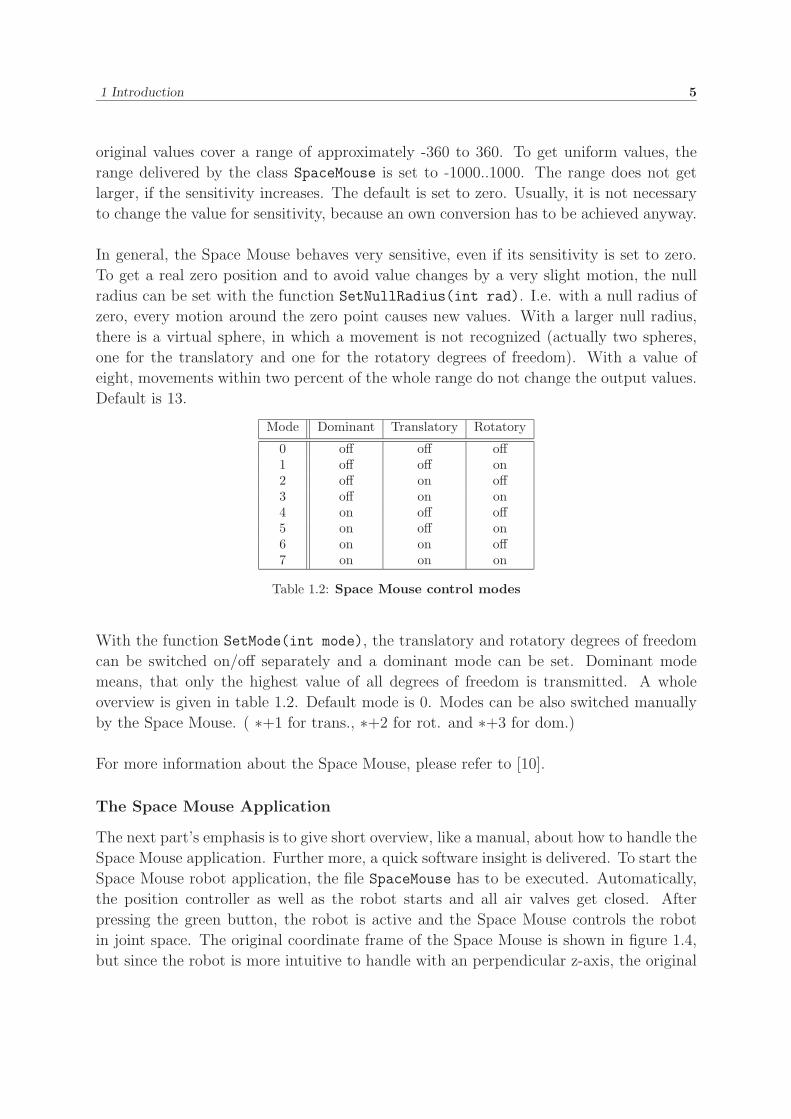
Mode Dominant Translatory Rotatory
0 off off off1 off off on2 off on off3 off on on4 on off off5 on off on6 on on off7 on on on
Table 1.2: Space Mouse control modes
With the function SetMode(int mode), the translatory and rotatory degrees of freedom
can be switched on/off separately and a dominant mode can be set. Dominant mode
means, that only the highest value of all degrees of freedom is transmitted. A whole
overview is given in table 1.2. Default mode is 0. Modes can be also switched manually
by the Space Mouse. ( ∗+1 for trans., ∗+2 for rot. and ∗+3 for dom.)
For more information about the Space Mouse, please refer to [10].
The Space Mouse Application
The next part’s emphasis is to give short overview, like a manual, about how to handle the
Space Mouse application. Further more, a quick software insight is delivered. To start the
Space Mouse robot application, the file SpaceMouse has to be executed. Automatically,
the position controller as well as the robot starts and all air valves get closed. After
pressing the green button, the robot is active and the Space Mouse controls the robot
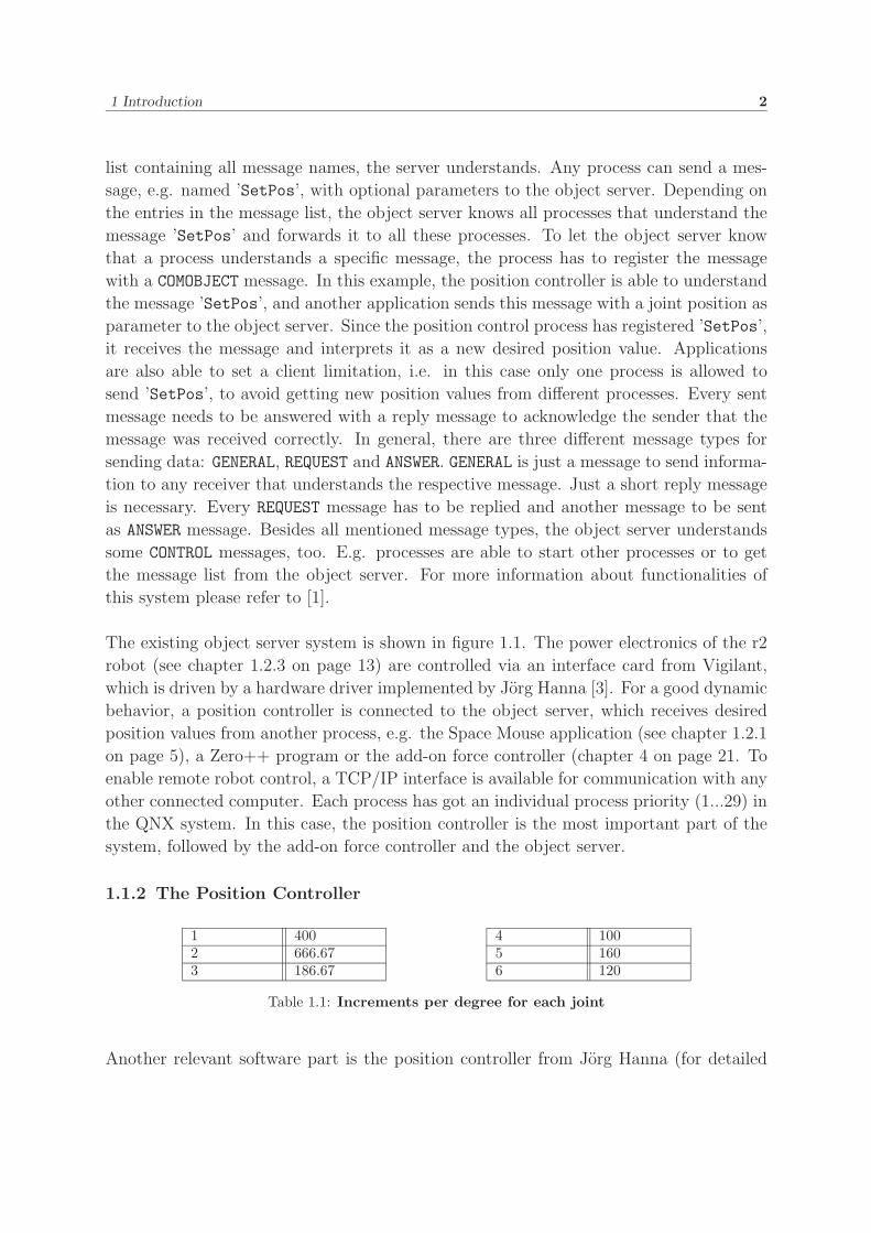
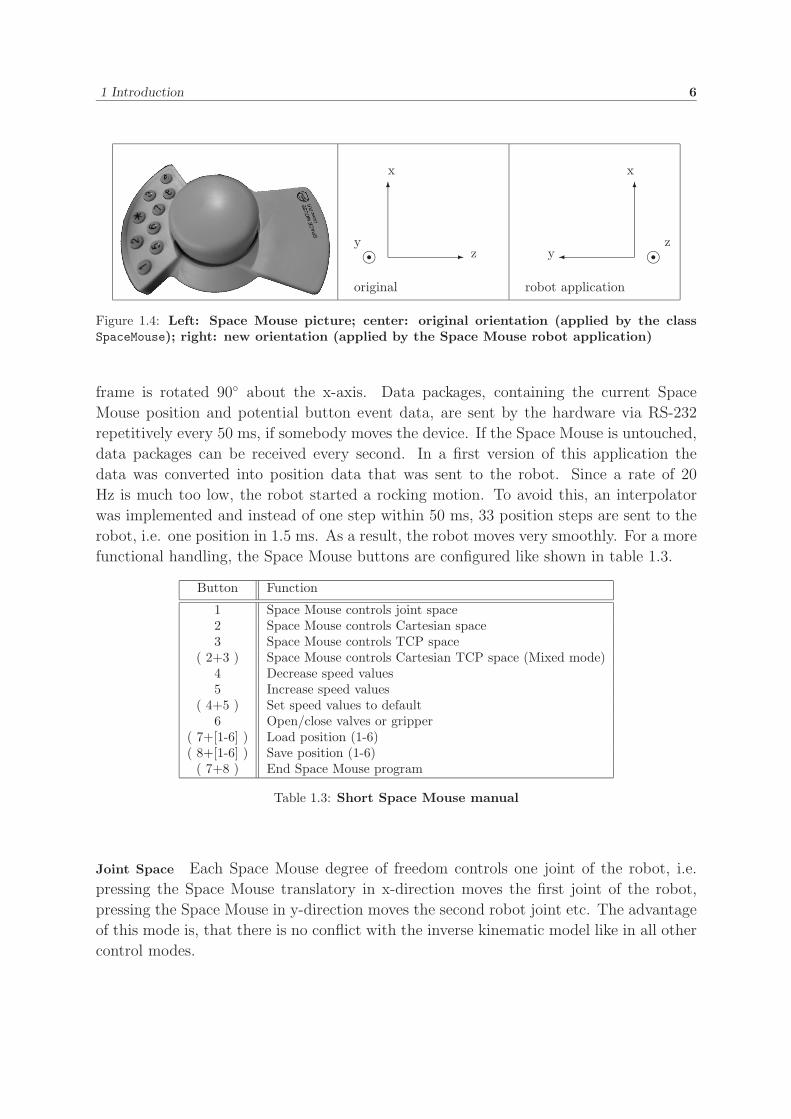
in joint space. The original coordinate frame of the Space Mouse is shown in figure 1.4,
but since the robot is more intuitive to handle with an perpendicular z-axis, the original
1 Introduction 6
�
� z
x
��y
original
�
�y
x
��z
robot application
Figure 1.4: Left: Space Mouse picture; center: original orientation (applied by the classSpaceMouse); right: new orientation (applied by the Space Mouse robot application)
frame is rotated 90◦ about the x-axis. Data packages, containing the current Space
Mouse position and potential button event data, are sent by the hardware via RS-232
repetitively every 50 ms, if somebody moves the device. If the Space Mouse is untouched,
data packages can be received every second. In a first version of this application the
data was converted into position data that was sent to the robot. Since a rate of 20
Hz is much too low, the robot started a rocking motion. To avoid this, an interpolator
was implemented and instead of one step within 50 ms, 33 position steps are sent to the
robot, i.e. one position in 1.5 ms. As a result, the robot moves very smoothly. For a more
functional handling, the Space Mouse buttons are configured like shown in table 1.3.
Button Function
1 Space Mouse controls joint space2 Space Mouse controls Cartesian space3 Space Mouse controls TCP space
( 2+3 ) Space Mouse controls Cartesian TCP space (Mixed mode)4 Decrease speed values5 Increase speed values
( 4+5 ) Set speed values to default6 Open/close valves or gripper
( 7+[1-6] ) Load position (1-6)( 8+[1-6] ) Save position (1-6)
( 7+8 ) End Space Mouse program
Table 1.3: Short Space Mouse manual
Joint Space Each Space Mouse degree of freedom controls one joint of the robot, i.e.
pressing the Space Mouse translatory in x-direction moves the first joint of the robot,
pressing the Space Mouse in y-direction moves the second robot joint etc. The advantage
of this mode is, that there is no conflict with the inverse kinematic model like in all other
control modes.
1 Introduction 7
Cartesian Space Button two switches to Cartesian control mode, i.e. the following trans-
formation is applied:
RTnew = TRotRPYSM · TTrans
SM · RTold
Where TRotRPYSM is a rotation frame containing the rotatory Space Mouse values, TTrans
SM
a translation frame that contains the translatory values and RTnew is the robot’s new
position w.r.t. the robot base frame, which is the reference frame. As a result the
absolute speed value for translatory movements is constant, but for rotatory movements
it depends on the distance to the corresponding rotation axis. To keep the absolute
velocity of the manipulator constant, a compensation factor, which contains the distance
to the respective axis, was integrated.
TCP Space Pressing button three puts the reference frame into the task frame, i.e. if
there is no tool, the task frame equals the tool center point frame (TCP), otherwise, there
is an offset frame TCPTTask that transforms the TCP frame to the task frame.
RTnew = RTold · TCPTTask · TTransSM · TRotRPY
SM · TCPTTask−1
Cartesian TCP Space (Mixed Mode) This control mode offers the most intuitive robot
control. Translatory movements are executed w.r.t. the robot base frame like in Cartesian
mode, but for rotatory movements the robot base frame is translatory shifted into the task
frame. As the separation of rotatory and translatory degrees of freedom are separated,
the transformation is more complex:
RTnew = RTTransold · TTrans
SM · RTRotRPYold · TCPTTrans
Task
· RTRotRPYold
−1 · TRotRPYSM · RTRotRPY
old · TCPTTransTask
−1
The syntax RTTransold means a translation frame, which contains only the old manipula-
tor position, but not its orientation. RTRotRPYold is the respective rotation frame of the
old manipulator position. This syntax is considered to rule for all other transformation
frames in the equation above. To comprehend the transformation completely a figure is
necessary, but since this document’s part is not the main one such an explanation was
abandoned.
1 Introduction 8
Several Other Functions The buttons four and five are responsible for the speed set
point, which can range from 1 to 100, default is 20. Pressing button four decreases the
speed by one integer, button five increases the speed. While pressing one of these buttons,
robot control is disabled. To accelerate speed setup, the Space Mouse’s head needs to
be touched and button four or five to be pressed. Attention: if the buttons are released
before the head of the Space Mouse, the robot may move unintentional. The default
speed value is set, when both buttons, four and five, are pressed simultaneously.
To open or close a gripper or to activate/deactivate a sucker, button six has to be hit.
To store a position, button eight and a number between one and six have to be pressed
simultaneously. To load a stored position, button seven and one of the numbers have
to be used. This way, the user is able to store six positions, which are available even
after ending the program, since they are stored in a file named ’pos.dat’. Hitting button
seven and eight simultaneously moves the robot to its default position, ends the position
controller and with it the robot and closes all valves.
Since there are still problems with the inverse kinematics, the user has to press the
∗-key when the robot needs to reconfigure itself. This way, the user is not appalled, if the
robot takes a new configuration. To disable this feature, the Space Mouse application
has to be started with the -e option.
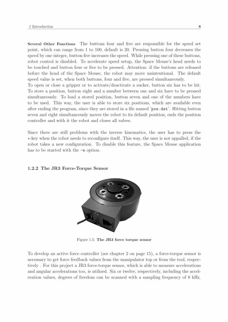
1.2.2 The JR3 Force-Torque Sensor
Figure 1.5: The JR3 force torque sensor
To develop an active force controller (see chapter 2 on page 15), a force-torque sensor is
necessary to get force feedback values from the manipulator top or from the tool, respec-
tively . For this project a JR3 force-torque sensor, which is able to measure accelerations
and angular accelerations too, is utilized. Six or twelve, respectively, including the accel-
eration values, degrees of freedom can be scanned with a sampling frequency of 8 kHz.
The signals are sent to a PC card that contains primarily a DSP and dual port RAM.
The 10 Mips DSP gets data from the sensor and transforms these data for the user, who
is able to determine a specific transformation from the center of the sensor to the task
frame. The resulting data is written into a dual port RAM that the DSP and the user
application can access simultaneously. Figure 1.5 shows the JR3 sensor. The top surface
is mounted on the robot’s manipulator and the bottom can be used for any tool. There
are two outlets to connect the sensor with the PC cards, the left one (with cable in fig-
ure 1.5) for force-torque data and the right one for acceleration values. The next part
describes the class FTS, which was implemented to drive the sensor. Afterwards a short
application example completes this section.
1 Introduction 10
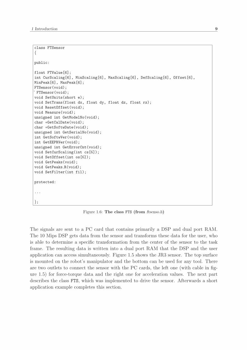
The Class FTS
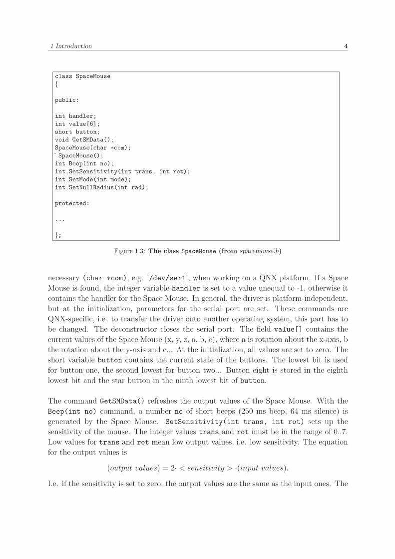
Figure 1.6 shows the source code of the respective class, afterwards the variable meanings
are described in table 1.4.
The constructor initializes the sensor: Model no, serial no, software version, software
release date, EEPROM version and the date of the last calibration are shown on screen
as well as the current offset and scaling values (i.e. default values). If there is no JR3 PC
card with sensor found, all values are set to -1. In a first version of the driver the values
for Offset[], MinScaling[], MaxScaling[] and DefScaling[] were set to default,
MinPeak[] and MaxPeak[] were read and reset, CurScaling[] was set to DefSacling[],
transformation was set to zero, units were set to international and filter two (125 Hz) was
activated. The disadvantage of this proceeding is the impossibility, to create a monitor
process, which is able to use the sensor values while another process (e.g. a controller)
uses the sensor either. As a result, this part of the initialization procedure was removed,
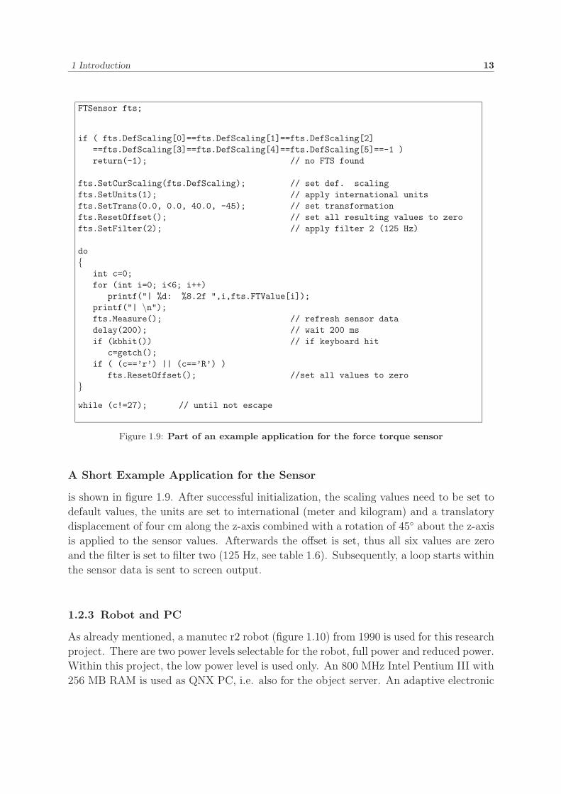
and the user application has to set up the sensor itself (see example in figure 1.9 on page
13). The deconstructor has no function. The command Measure() refreshes the sensor
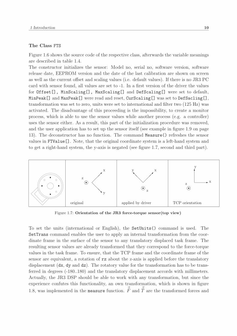
values in FTValue[]. Note, that the original coordinate system is a left-hand system and
to get a right-hand system, the y-axis is negated (see figure 1.7, second and third part).
����
����
x
y
��z
original
����
���
xy
��z
applied by driver
�
�y
x��
z
TCP orientation
Figure 1.7: Orientation of the JR3 force-torque sensor(top view)
To set the units (international or English), the SetUnits() command is used. The
SetTrans command enables the user to apply an internal transformation from the coor-
dinate frame in the surface of the sensor to any translatory displaced task frame. The
resulting sensor values are already transformed that they correspond to the force-torque
values in the task frame. To ensure, that the TCP frame and the coordinate frame of the
sensor are equivalent, a rotation of rz about the z-axis is applied before the translatory
displacement (dx, dy and dz). The rotatory value for the transformation has to be trans-
ferred in degrees (-180..180) and the translatory displacement accords with millimeters.
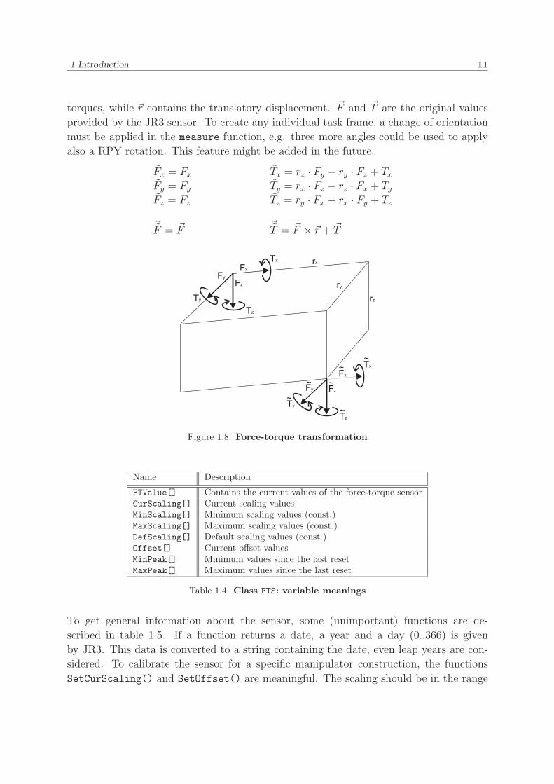
Actually, the JR3 DSP should be able to work with any transformation, but since the
experience confutes this functionality, an own transformation, which is shown in figure
1.8, was implemented in the measure function. �F and �T are the transformed forces and
1 Introduction 11
torques, while �r contains the translatory displacement. �F and �T are the original values
provided by the JR3 sensor. To create any individual task frame, a change of orientation
must be applied in the measure function, e.g. three more angles could be used to apply
also a RPY rotation. This feature might be added in the future.
Fx = Fx Tx = rz · Fy − ry · Fz + Tx
Fy = Fy Ty = rx · Fz − rz · Fx + Ty
Fz = Fz Tz = ry · Fx − rx · Fy + Tz
�F = �F �T = �F × �r + �T
Figure 1.8: Force-torque transformation
Name Description
FTValue[] Contains the current values of the force-torque sensorCurScaling[] Current scaling valuesMinScaling[] Minimum scaling values (const.)MaxScaling[] Maximum scaling values (const.)DefScaling[] Default scaling values (const.)Offset[] Current offset valuesMinPeak[] Minimum values since the last resetMaxPeak[] Maximum values since the last reset
Table 1.4: Class FTS: variable meanings
To get general information about the sensor, some (unimportant) functions are de-
scribed in table 1.5. If a function returns a date, a year and a day (0..366) is given
by JR3. This data is converted to a string containing the date, even leap years are con-
sidered. To calibrate the sensor for a specific manipulator construction, the functions
SetCurScaling() and SetOffset() are meaningful. The scaling should be in the range
1 Introduction 12
Name Description
GetModelNo() Returns the model number of the sensorGetCalDate() To get the last date of calibration (e.g. ’January 8 2001’)GetSoftwDate() Delivers the release date of the software (e.g. ’September 3 1996’)GetSerialNo() Interrogates the serial numberGetSoftwVer() Returns the software versionGetEEPRVer() To get the EEPROM version
Table 1.5: Class FTS: function description
given by MinScaling[] and MaxScaling[]. The command ResetOffset() takes the
values from filter two and changes the offset values such that the values of FTValue[] are
zero. This function is not really necessary, but it makes the chore much simpler. During
one of the commands to set scaling or offset, the DSP is busy for a short time interval,
i.e. refreshing the sensor values will be delayed. Depending on the circumstances, the
sensor works at, a low-pass filter has to be set. If the variable Filter is zero, no filter is
active. This value can be set via the method SetFilter(), as shown in table 1.6.
Fx 200 N 400 NFy 200 N 400 NFz 400 N 800 NTx 12 Nm 24 NmTy 12 Nm 24 NmTz 12 Nm 24 Nm
Table 1.7: JR3 Force-torque sensor: maximum forces and torques
To be sure, that the user recognizes every peak value, two special functions, GetPeaks()
and GetPeaks R(), are implemented. GetPeaks() refreshes the values MinPeak[] and
MaxPeak[] as well as GetPeaks R() does, but GetPeaks R() resets the original values to
start again with zero values. I.e. with GetPeaks R() the user receives values since the
last call, and with GetPeaks() the values since the initialization or since the last reset
with GetPeaks R(), respectively, are returned. All peak values depend on the filter (0..6),
i.e. when changing the filter, the peak values are reset. During one of the GetPeak com-
mands, the JR3 DSP is busy for a certain time, i.e. refreshing the sensor values is delayed.
1 Introduction 13
FTSensor fts;
if ( fts.DefScaling[0]==fts.DefScaling[1]==fts.DefScaling[2]==fts.DefScaling[3]==fts.DefScaling[4]==fts.DefScaling[5]==-1 )return(-1); // no FTS found
fts.SetCurScaling(fts.DefScaling); // set def. scalingfts.SetUnits(1); // apply international unitsfts.SetTrans(0.0, 0.0, 40.0, -45); // set transformationfts.ResetOffset(); // set all resulting values to zerofts.SetFilter(2); // apply filter 2 (125 Hz)
do{
int c=0;for (int i=0; i<6; i++)
printf("| %d: %8.2f ",i,fts.FTValue[i]);printf("| \n");fts.Measure(); // refresh sensor datadelay(200); // wait 200 msif (kbhit()) // if keyboard hit
c=getch();if ( (c==’r’) || (c==’R’) )
fts.ResetOffset(); //set all values to zero}while (c!=27); // until not escape
Figure 1.9: Part of an example application for the force torque sensor
A Short Example Application for the Sensor
is shown in figure 1.9. After successful initialization, the scaling values need to be set to
default values, the units are set to international (meter and kilogram) and a translatory
displacement of four cm along the z-axis combined with a rotation of 45◦ about the z-axis
is applied to the sensor values. Afterwards the offset is set, thus all six values are zero
and the filter is set to filter two (125 Hz, see table 1.6). Subsequently, a loop starts within
the sensor data is sent to screen output.
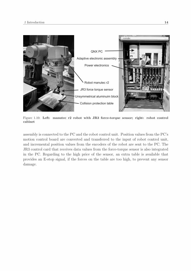
1.2.3 Robot and PC
As already mentioned, a manutec r2 robot (figure 1.10) from 1990 is used for this research
project. There are two power levels selectable for the robot, full power and reduced power.
Within this project, the low power level is used only. An 800 MHz Intel Pentium III with
256 MB RAM is used as QNX PC, i.e. also for the object server. An adaptive electronic
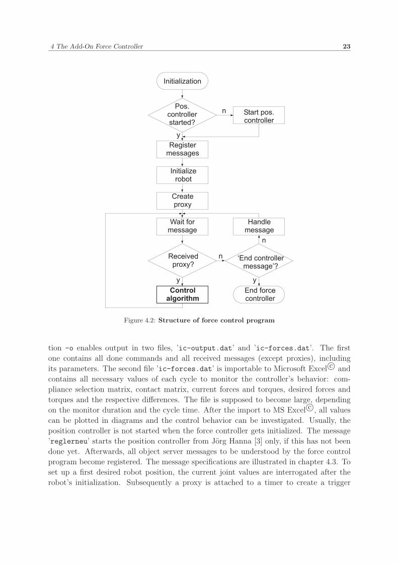
can be plotted in diagrams and the control behavior can be investigated. Usually, the
position controller is not started when the force controller gets initialized. The message
’reglerneu’ starts the position controller from Jorg Hanna [3] only, if this has not been
done yet. Afterwards, all object server messages to be understood by the force control
program become registered. The message specifications are illustrated in chapter 4.3. To
set up a first desired robot position, the current joint values are interrogated after the
robot’s initialization. Subsequently a proxy is attached to a timer to create a trigger
4 The Add-On Force Controller 24
signal, which occurs every two milliseconds, the force control cycle time. This factor is
very important. For better results a lower cycle time would surely bid better control
behavior, but since the behavior of the QNX PC is not deterministic for such values,
two milliseconds was chosen. The last command before the real control algorithm is the
sensor reset to get suggestive force-torque values. An endless loop, which can only be
interrupted by the ’EndICtrl’ message, starts and waits for a message. There are only
two kinds of messages that can be received: a proxy message or a message from the ob-
ject server. After the reception of a proxy message, the control algorithm (chapter 4.2) is
applied, respectively after reception of an object server message, it is handled as shown
in chapter 4.3.
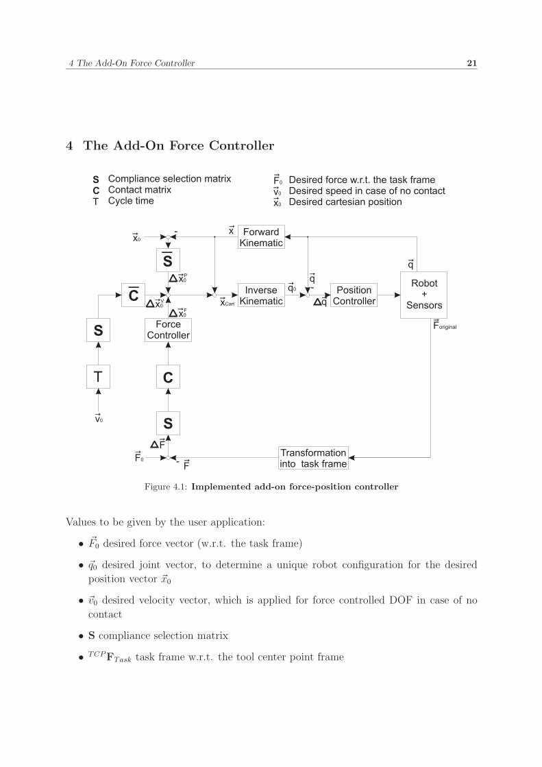
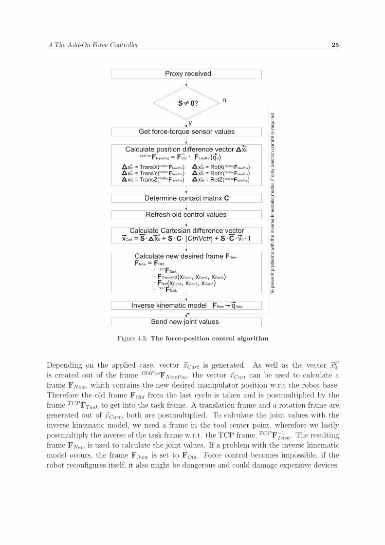
4.2 Control Algorithm
The bold block ’Control algorithm’ of the program flow chart shown in figure 4.2 is detailed
in this section. If a proxy message is received, one control cycle begins. One principal
weakness of the chosen control concept is the inverse kinematic model, whose result is not
unique for every frame. As already mentioned on page 22, the desired position is given in
joint values instead of a Cartesian position, i.e. if no force control (S = 0) is demanded,
the position values are looped through and are sent straight to the position controller.
If at least one DOF is force controlled, force-torque values are interrogated and a frameOldPosFNewPos is calculated. Here, only the desired position frame and the old position
from the last cycle are eyed to calculate this difference frame. The translatory fraction
(xP01
, xP02
, xP03
) as well as the rotatory one (xP04
, xP05
, xP06
) are stored in a position difference
vector �xP0 . The current sensor values are used to determine the diagonal six by six contact
matrix C. The discrete PID controller is described in chapter 4.4. Such a discrete PID
controller needs the controller input values from the last two cycles and the controller
output values from the last cycle. Thus, the old values are stored or the corresponding
variables are refreshed, respectively . Within the next step a Cartesian difference vector
�xCart is generated. This vector contains the Cartesian difference from the old position
of the last cycle to the new position of the current cycle. Depending on the compliance
selection matrix and the contact matrix, three cases can be distinguished:
1. The compliance selection matrix S for the corresponding DOF is zero, i.e. this DOF
is only position controlled.
2. The S matrix element for the corresponding DOF is one and the respective element
of the contact matrix C is zero, i.e. the DOF is force controlled, but the control
loop is not closed. For this case the corresponding velocity value of �v0 is applied.
3. The corresponding elements of S and C are both one, i.e. the force control loop for
this DOF is closed and the PID controller rules.
4 The Add-On Force Controller 25
Figure 4.3: The force-position control algorithm
Depending on the applied case, vector �xCart is generated. As well as the vector �xP0
is created out of the frame OldPosFNewPos, the vector �xCart can be used to calculate a
frame FNew, which contains the new desired manipulator position w.r.t the robot base.
Therefore the old frame FOld from the last cycle is taken and is postmultiplied by the
frame TCPFTask to get into the task frame. A translation frame and a rotation frame are
generated out of �xCart, both are postmultiplied. To calculate the joint values with the
inverse kinematic model, we need a frame in the tool center point, wherefore we lastly
postmultiply the inverse of the task frame w.r.t. the TCP frame, TCPF−1Task. The resulting
frame FNew is used to calculate the joint values. If a problem with the inverse kinematic
model occurs, the frame FNew is set to FOld. Force control becomes impossible, if the
robot reconfigures itself, it also might be dangerous and could damage expensive devices.
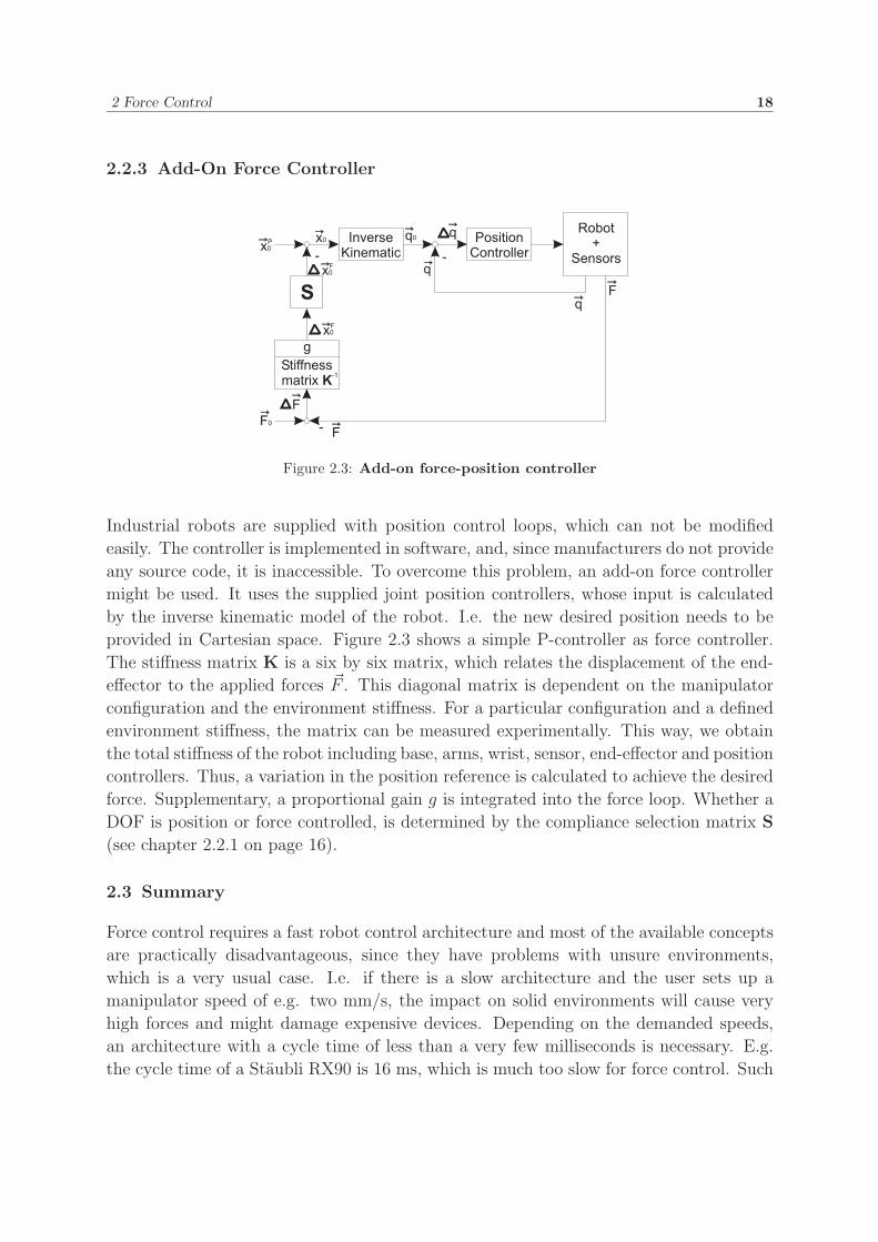
4 The Add-On Force Controller 26
Usually the inverse kinematic model is unique, and thus, the obtained joint values are
sent to the position controller.
4.3 Messages
Only the described control algorithm is insufficient for the user application, since more
control commands are necessary for a convenient user application. Besides a message
that contains the new desired set point (position, force, velocity in case of no contact and
compliance selection matrix), ’SetFPV’ (set force position value), some more messages
are necessary, e.g. to end the force controller, to setup the task frame and to get current
force-torque values. The fact, that the robot is an object of the r2 class and that the user
application program as well as the force control program needs access to the robot, is a
problem. There are two solutions: either a pointer to the r2 object is transmitted from the
force controller to the user application (or vice versa) or all required commands need to
be implemented. The second solution was chosen and three extra messages provide robot
commands: ’RobotMove’, ’SetRobotConf’ and ’GetCurPos’. A survey of all messages is
presented below.
EndICtrl
This simple GENERAL message ends the force-position controller, i.e. the force control
program ends the position controller, logs off from the object server and ends itself.
SetFPV
This is one of the most important messages, its type is also GENERAL, since no answer
is required. ’SetFPV’ is similar to the ’SetPos’ message (set position) for the position
controller, but instead of one parameter, four parameters are attached:
1. Six integer elements containing the desired joint values (i.e. the position) in incre-
ments.
2. A six-dimensional field of floating-point numbers, which contains the desired force
values in N for each DOF w.r.t. the task frame.
3. A single integer value, whose bits represent the diagonal elements of the compliance
selection matrix S. The least significant bit represents the first element of S etc.
4. Lastly, a vector that contains six velocities for the case of force control without
contact. These six floating-point values must be given in mm/s.
4 The Add-On Force Controller 27
SetTCPOffset
For a translatory displacement of the task frame w.r.t the tool center point frame, the
GENERAL message ’SetTCPOffset’ is used. Note: only a translatory displacement can be
applied, for another orientation, this command has to be expanded by RPY angles for
example, but this feature is supposed to be implemented in future time. A field of three
floating-point values has to be attached to this message. Each value represents the trans-
latory displacement in millimeters. On the basis of these magnitudes, a transformation
frame TCPFTask is generated and the sensor values are transformed into the task frame.
Desired forces are controlled in this frame.
If another program monitors the sensor values, this transformation is not applied, since
it is executed by the measure function of the FTS class and not by the JR3 DSP. For
correct monitor values, a pointer to the corresponding FTS object has to be sent to the
monitor program, which just has to interrogate the variable FTValue.
SetRotZ
If the coordinate systems are twisted by 45◦, it has to be compensated by this function,
that both, the manipulator frame and the force-torque sensor frame, are orientated in
the same manner. I.e. to obtain a force-torque sensor frame, which is coincident with the
tool center point frame, a rotation about the z-axis is applied. The angle in degrees about
the z-axis is attached to this message as integer value. In comparison to ’SetTCPOffset’
the transformation of this GENERAL message is executed by the JR3 DSP, i.e. a monitor
programm can eye the same values. Actually a rotation about the z-axis does not hit
every case, but for the r2 robot this simple transformation is enough. For any future
upgrades with more parameters, remember, that the JR3 DSP has problems with complex
transformations (see chapter 1.2.2 on page 8). Of course, this transformation is applied
before the transformation initialized by the ’SetTCPOffset’ message.
RobotMove
The original Move command of the r2 class needs to be replaced to enable the user
application smooth robot movements to a defined position. To acknowledge the user
application, when the movement is complete, the ’RobotMove’ message is a REQUEST
message. After reception of this message, the timer, which is attached to a proxy, is
disarmed and the Move command is executed. Its parameters are transferred with the
’RobotMove’ message as joint values, i.e. six floating-point magnitudes in radians. After
the complete movement, an ANSWER message with the current position is sent to the object
server and the timer is rearmed.
4 The Add-On Force Controller 28
SetRobotConf
Before the inverse kinematic model can be applied, the Denavit-Hartenbeg parameters
as well as acceleration and deceleration parameters need to be transmitted to the force
controller. All parameters are sent via this GENERAL message.
GetFTSValues
To provide the force feedback values to the user application, the REQUEST message ’GetFTSValues’
is applied. The ANSWER message is attended by a six-tuple of floating-point values con-
taining the current forces and torques that are measured in the respective task frame.
FTSReset
Another GENERAL message is ’FTSReset’, which zeroizes the force-torque values from the
sensor to get useful values for force control. This command should be achieved right
before force control is enabled.
GetCurPos
Actually, this REQUEST message equals the ’AktPos’ message provided by the position
controller. The user application sends this message, and the attachment of the ANSWER
contains six joint values in increments.
SetCtrlPara
During the setup of the control parameters (see chapter 4.4), the parameters themselves
had to be varied. Thus, a dynamic change of these parameters is necessary and is enabled
by this GENERAL message. A six-tuple of floating-point values, which contains the P-values,
the I-times and the D-times of the force as well as of the torque controller is attached as
parameter. Matching parameters are applied by default, i.e. it is not recommended to
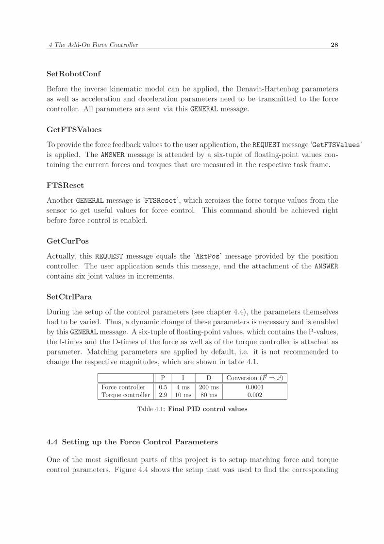
change the respective magnitudes, which are shown in table 4.1.
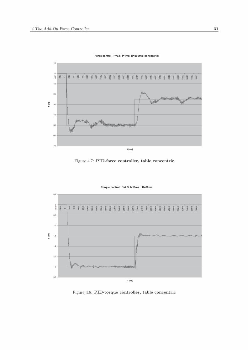
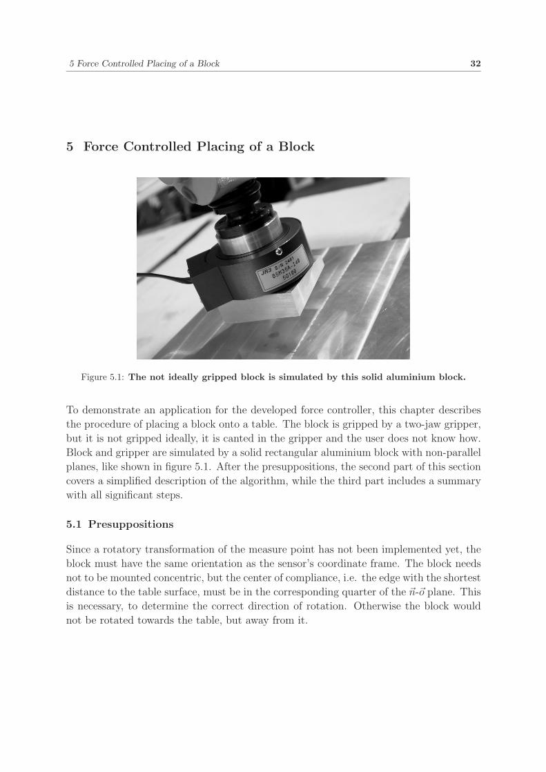
P I D Conversion (�F ⇒ �x)Force controller 0.5 4 ms 200 ms 0.0001Torque controller 2.9 10 ms 80 ms 0.002
Table 4.1: Final PID control values
4.4 Setting up the Force Control Parameters
One of the most significant parts of this project is to setup matching force and torque
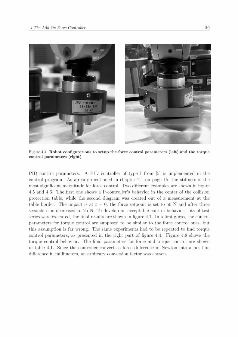
control parameters. Figure 4.4 shows the setup that was used to find the corresponding
4 The Add-On Force Controller 29
Figure 4.4: Robot configurations to setup the force control parameters (left) and the torquecontrol parameters (right)
PID control parameters. A PID controller of type I from [5] is implemented in the
control program. As already mentioned in chapter 2.1 on page 15, the stiffness is the
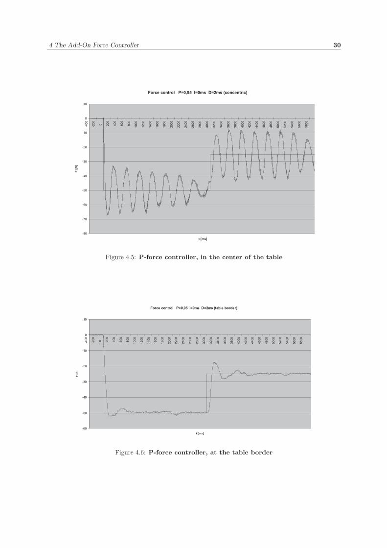
most significant magnitude for force control. Two different examples are shown in figure
4.5 and 4.6. The first one shows a P-controller’s behavior in the center of the collision
protection table, while the second diagram was created out of a measurement at the
table border. The impact is at t = 0, the force setpoint is set to 50 N and after three
seconds it is decreased to 25 N. To develop an acceptable control behavior, lots of test
series were executed, the final results are shown in figure 4.7. In a first guess, the control
parameters for torque control are supposed to be similar to the force control ones, but
this assumption is far wrong. The same experiments had to be repeated to find torque
control parameters, as presented in the right part of figure 4.4. Figure 4.8 shows the
torque control behavior. The final parameters for force and torque control are shown
in table 4.1. Since the controller converts a force difference in Newton into a position
difference in millimeters, an arbitrary conversion factor was chosen.
4 The Add-On Force Controller 30
Figure 4.5: P-force controller, in the center of the table
Figure 4.6: P-force controller, at the table border
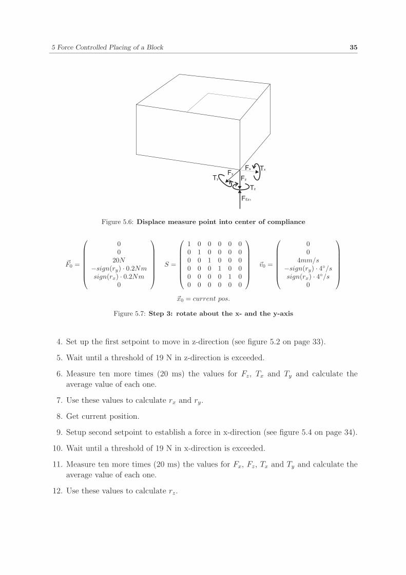
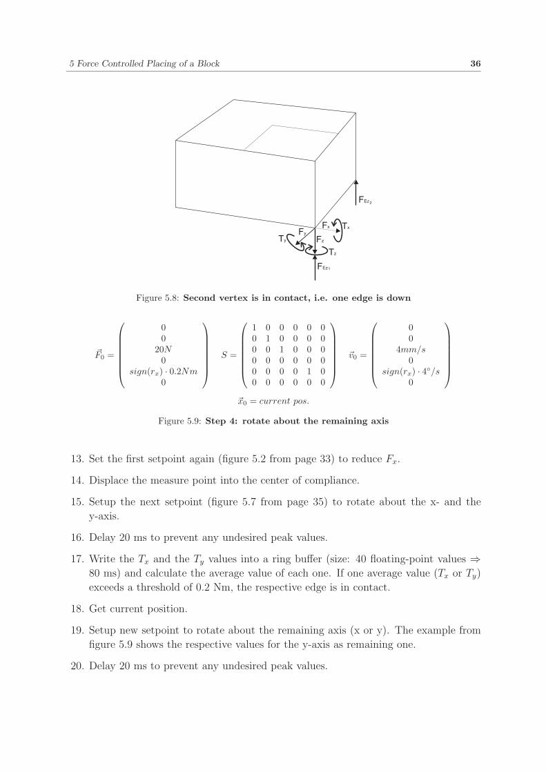
Figure 5.9: Step 4: rotate about the remaining axis
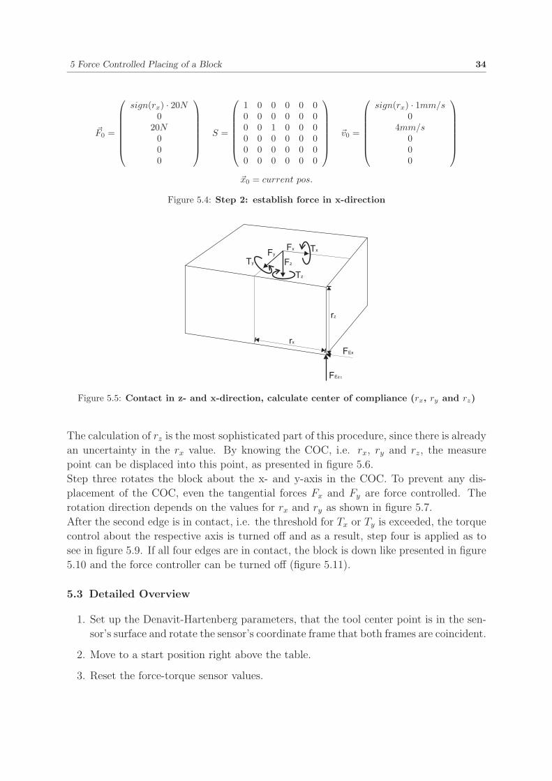
13. Set the first setpoint again (figure 5.2 from page 33) to reduce Fx.
14. Displace the measure point into the center of compliance.
15. Setup the next setpoint (figure 5.7 from page 35) to rotate about the x- and the
y-axis.
16. Delay 20 ms to prevent any undesired peak values.
17. Write the Tx and the Ty values into a ring buffer (size: 40 floating-point values ⇒80 ms) and calculate the average value of each one. If one average value (Tx or Ty)
exceeds a threshold of 0.2 Nm, the respective edge is in contact.
18. Get current position.
19. Setup new setpoint to rotate about the remaining axis (x or y). The example from
figure 5.9 shows the respective values for the y-axis as remaining one.
20. Delay 20 ms to prevent any undesired peak values.