Freie Universität Berlin Fachbereich Geowissenschaften Institut für Geographische Wissenschaften Physische Geographie Masterarbeit M. Sc. Geographie (Terrestrische Systeme) Soil Erosion Risk Assessment in the Upper Mefou Subcatchment, Southern Cameroon Plateau Application of the RUSLE3D in the humid tropics in the immediate vicinity of Yaoundé Fabian Becker Erstgutachterin: Prof. Dr. Brigitta Schütt Zweitgutachter: Prof. Dr. Tilman Rost Berlin, 11. Februar 2015
Transcript
Freie Universität BerlinFachbereich Geowissenschaften
Institut für Geographische WissenschaftenPhysische Geographie
Soil Erosion Risk Assessment in the Upper Mefou Subcatchment,Southern Cameroon Plateau
Application of the RUSLE3D in the humid tropics in the immediate vicinityof Yaoundé
Fabian Becker
Erstgutachterin: Prof. Dr. Brigitta SchüttZweitgutachter: Prof. Dr. Tilman Rost
Berlin, 11. Februar 2015
AcknowledgementsI would like to express my very great appreciation to my supervisor at Freie UniversitätBerlin, Prof. Dr. Brigitta Schütt, for constructive suggestions, helpful ideas and motivatingcomments. For co-supervision and various discussions, I am thankful to Prof. Dr. Karl TilmanRost (Freie Universität Berlin).During field work in November and December 2012 I met a lot of people from Université deYaoundé I who helped me and were open for discussion: Rodrigue Aime Feumba, MauriceOlivier Zogning Moffo, Alain Tchamagam Touko, Ruphine Lydie Mbezele Atengana, andProf. Dr. Nicolas Gabriel Andjica (Director de Ecole Normale Superieure). I would also liketo thank the people in the Upper Mefou subcatchment who where open to the field workwithin the project, especially the chiefs of the villages who made fieldwork more bearable.I wish to acknowledge the discussions during the “IWM for Upper Mefou Sub-catchment”-workshop at the Higher Teachers Training College in Yaoundé in 2013. Dr. Stefan Thiemann(IWM Expert GmbH, Kempten, Germany) and Anette Stumptner provided assistance duringfield work and at Freie Universität.Special thanks should be offered to all colleagues at Freie Univeristät Berlin. Methodologicalassistance and patience of Dr. Philipp Hoelzmann and M. Scholz from the Laboratory ofPhysical Geography were necessary for soil analysis—especially for the preparation of grainsize samples.My special thanks are extended to Norbert Anselm. A comprehensive exchange of ideas andsome critical comment helped a lot to process data for the thesis, not to mention some hintswhich avoided spending hours in R or Latex forums.To come to an end, I would like to thank Susanne and Heinz-Wilhelm Becker.
The author was financially supported by the German Academic Exchange Service (DAAD,Deutscher Akademischer Austauschdienst) through the university cooperation programme“Welcome to Africa” in the project Integrated Watershed Management Research and Devel-opment Capacity Building (IWM R&D CB) (2012–2015). The project is headed by FreieUniversitát Berlin; partners are Kenyatta University, Nairobi, Kenya, University of YaoundéI, Cameroon, University of Cape Town, South Africa, and United Nations University, Bonn,Germany.
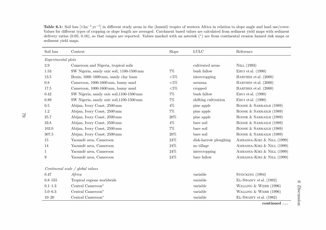
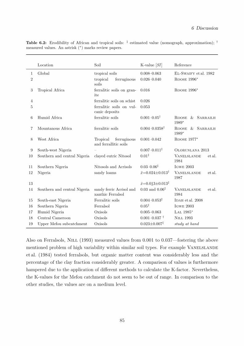
6.1 Soil loss in western Africa . . . . . . . . . . . . . . . . . . . . . . . . . . . . 796.2 Erodibility of African and tropical soils . . . . . . . . . . . . . . . . . . . . . 856.3 Influence of selected LS rill-to-interrill parameter on soil loss . . . . . . . . . 97
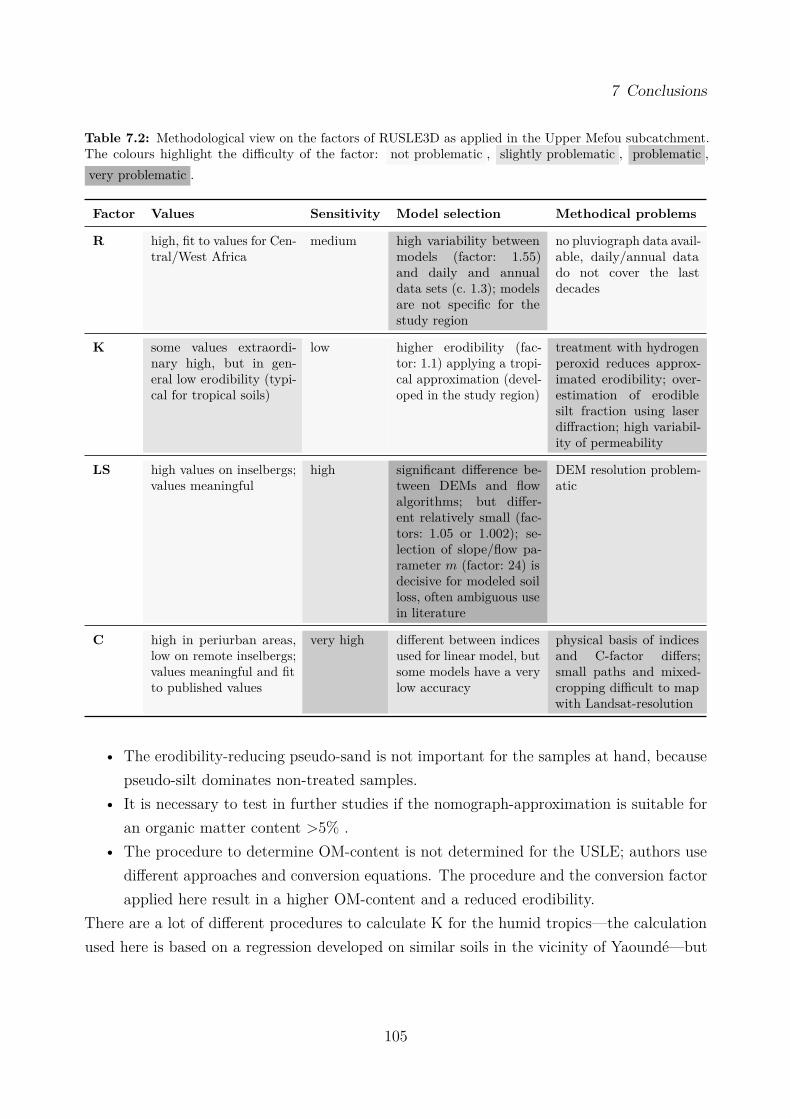
7.1 Summary: Erosion risk and recommended conservation measures . . . . . . . 1027.2 Methodolocial view on the factors of the RUSLE3D . . . . . . . . . . . . . . 105
List of Acronyms
ABAG Allgemeine Bodenabtragsgleichung (German for USLE)ARESED African Rainfall Erosivity Subregional Empirical DownscalingARS (United States Department of Agriculture) Agricultural Research ServiceASTER Advanced Spaceborne Thermal Emission and Reflection RadiometerC Cover and management factor (USLE)dBD dry Bulk Density (of sediments)D∞ Deterministic InfinityD8 Deterministic 8DEM Digital Elevation ModelDI Disturbance IndexDN Digital NumberETM+ (Landsat) Enhanced Thematic Mapper PlusFAO Food and Agriculture Organization (of the United Nations)GIS Geographic Information SystemIR InfraredIWM Integrated Watershed ManagementK Soil erodibility (USLE)KNMI Koninkijk Nederlands Meterologisch InstituutLS Slope angle and slope length factor (Topographic factor of the USLE)LULC Land Use and Land CoverLULCC Land Use and Land Cover ChangeMBA Multilevel B-Spline ApproximationMETI (Japan’s) Ministry of Economy, Trade and IndustryMFD Multiple Flow DirectionMFI Modified Fournier IndexMNT Modèle numérique de terrain (Digital Elevation Model)NASA (United States) National Aeronautics and Space AdministrationNDVI Normalized Difference Vegetation IndexNk Nkolbission (sample identifier)NSSH National Soil Survey Handbook (USDA)OC Organic Carbon
OFAT One-factor-at-a-time (sensitivity analysis)OLI Operational Land ImagerOM Organic MatterP Soil conservation factor (USLE)QA Quality Assessment (band of Landsat 8)R (programming language)R Rainfall erosivity factor (USLE)RSAGA R–System-for-Automated-Geoscientific-AnalysesRUSLE Revisited Universal Soil Loss EquationRUSLE3D threedimentional enhancement of the RUSLESAGA System for Automated Geoscientific AnalysesSDR Sediment Delivery RatioSEM Standard Error of the MeanSI Le Système International d’Unités, International System of UnitsSRTM Shuttle Radar Topography MissionSSY (Area) Specific Sediment YieldTC Total CarbonTCT Tasseled Cap TransformationsTIC Total Inorganic CarbonTOC Total Organic CarbonUS United States (of America, USA)USDA United States Department of AgricultureUSLE Universal Soil Loss EquationUSPED Unit Stream Power Erosion/DepositionWMO World Meteorological OrganizationWRS Worldwide Reference System (a global notion system for Landsat data)
IX
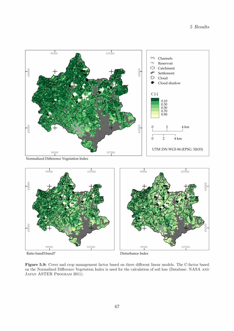
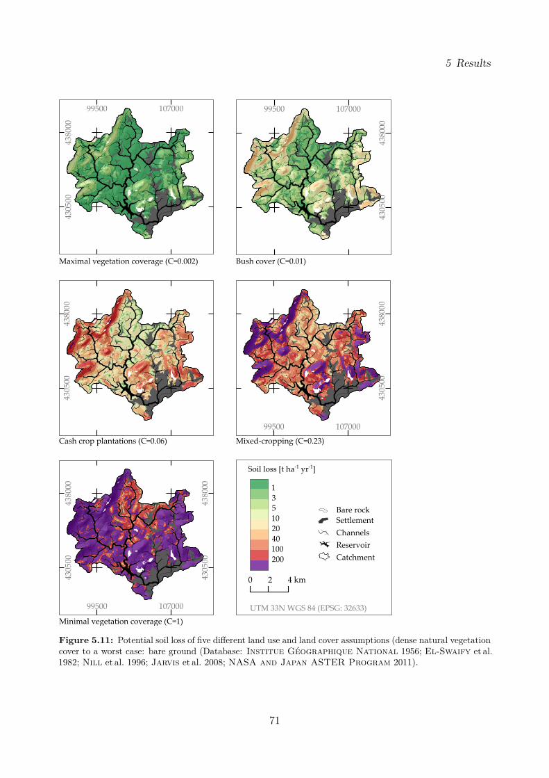
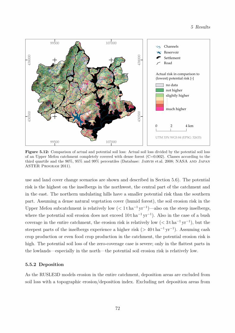
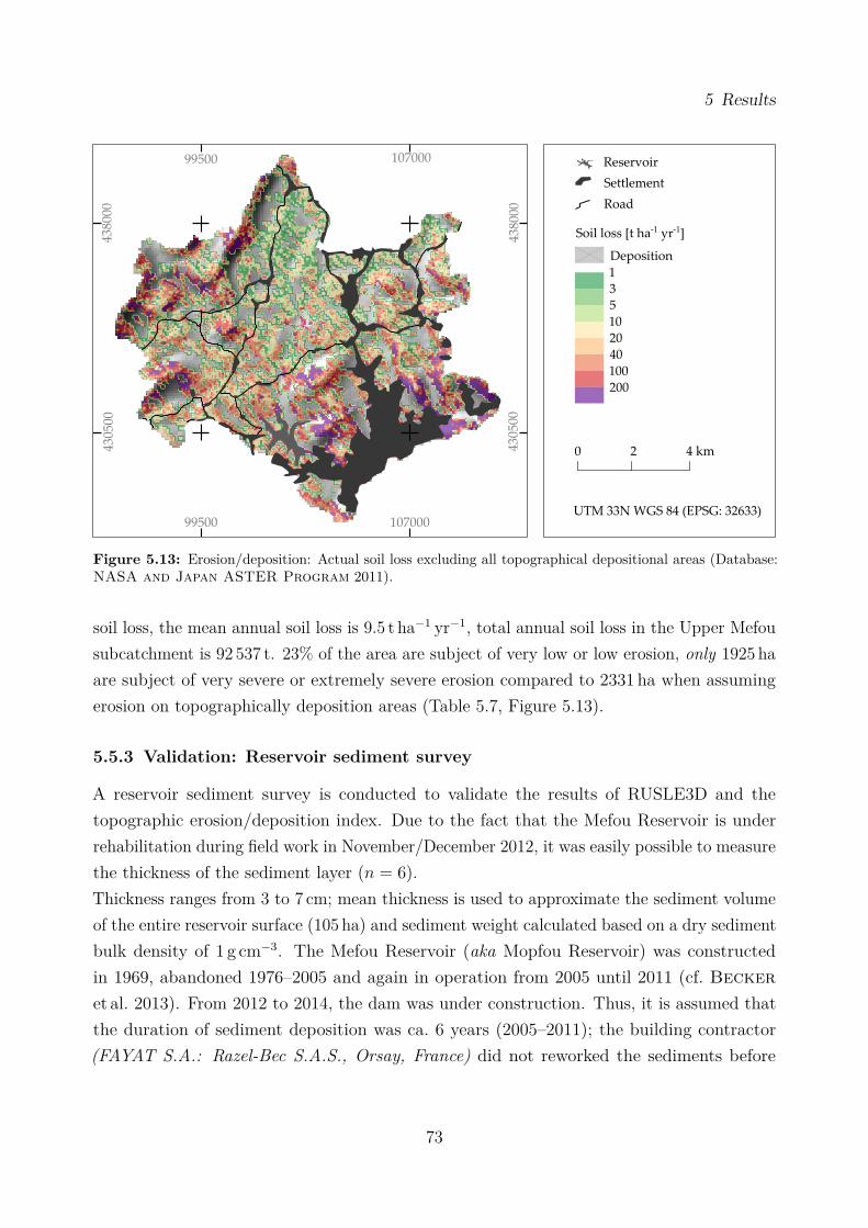
AbstractIn the humid tropics of the Southern Cameroon Plateau, the soil erosion risk (by water) isprincipally low to do a dense natural vegetation cover and a low erodibility of the “pseudo-sandy” soils. But due to deforestation and urban growth, land use is intensified and the soilerosion risk accelerated.In this context, the objective of the study at hand is firstly to assess the actual and potentialsoil erosion risk in the Upper Mefou subcatchment in the intermediate vicinity of Yaoundé.Secondly, the future risk is estimated based on four land use intensification scenarios and anassumed forest regrowth. The third objective is to discuss the applicability of a USLE-familymodel on the Southern Cameroon Plateau.Soil erosion risk is assessed using a three-dimensional enhancement of the ULSE, the RUSLE3D.An algebraic approximation of the USLE nomograph—adapted to tropical soils—is used toestimate soil erodibility (K): Grain size is measured using laser diffraction, organic matterusing an CNS-analyser and a carmhograph. Permeability is calculated on the basis of fieldmeasurements of infiltration rates using a minidisk infiltrometer. A linear model for thedaily rainfall–erosivity relationship from southeast Nigeria is applied to calculate the rainfallerosivity factor R. The cover and crop management factor C is modelled on the basis of alinear relationship between the NDVI of a Landsat 8 scene and ground truth values of C.The topographic potential factor LS is calculated on the basis of a SRTM Digital ElevationModel, where upslope contributing area is used instead of the USLE’s slope-length parameter.Deposition areas are masked using an erosion/deposition topographic index based on theunit stream power theory. The model accuracy is tested using the results of a reservoirsedimentation survey of the Mefou Reservoir and a one-factor-at-a-time sensitivity analysis.(1) In comparison to other studies in the humid tropics of Africa, modelled soil losses arerelatively high, but in the same order of magnitude. The validation shows that soil lossis somewhat overestimated. The high values might be explained by the steep relief of theinselbergs, which are pronounced in comparison to the relief Southern Cameroon Plateau.Rainfall is highly erosive, also when field preparation for cassava cultivation is still ongoing.The acutal erosion risk is especially high in periurban areas and around the Mefou Reservoir,where short-duration fallowing takes place and land use is more intensive, e. g. maize ormanioc monocropping. (2) The simulation of deforestation, land use intensification and anincrease in cash crop production is expected to result in a severe increase of soil loss, againespecially around Yaoundé and the reservoir, but also in the present rural areas. (3) An
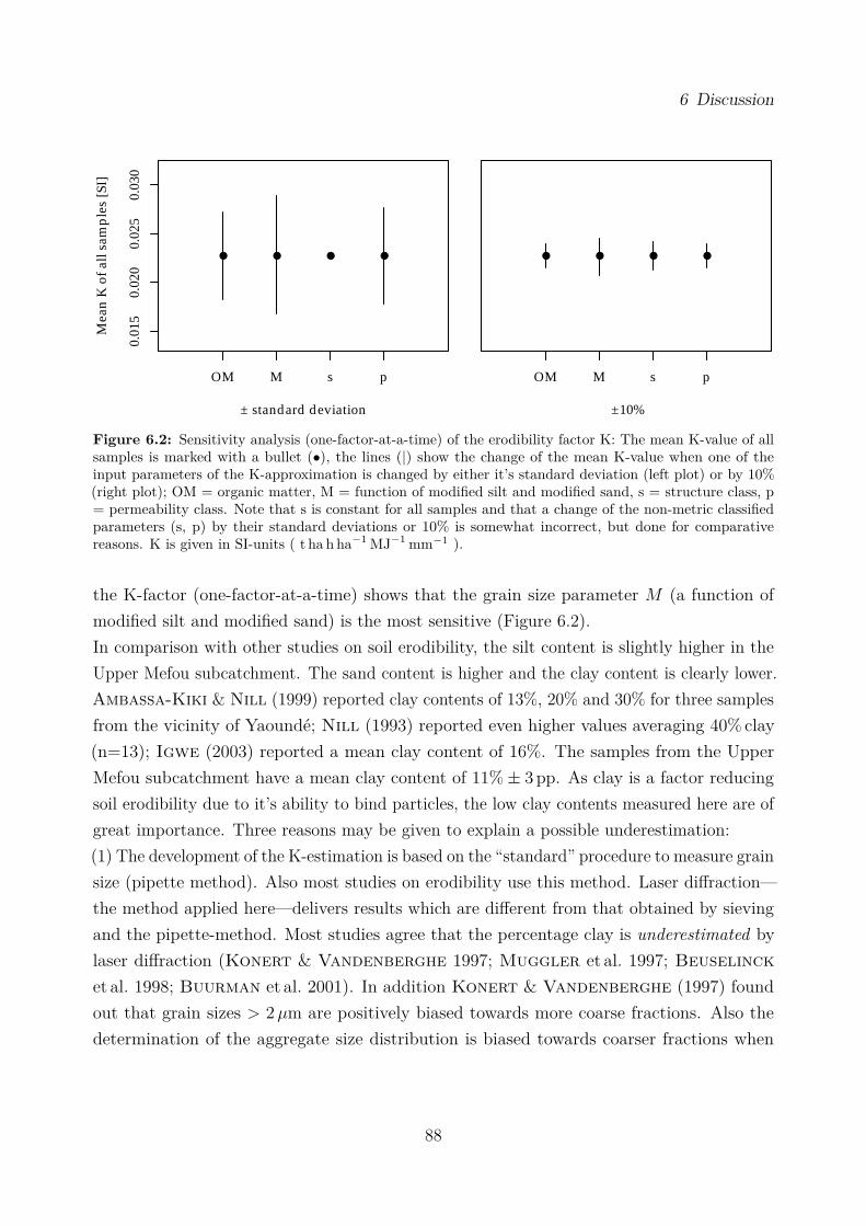
overestimation of soil loss might be attributed to a method inherent overestimation of thesilt and fine sand fraction by laser diffraction and a lack of observance of microaggregatesin the calculation of soil erodibility. The parameters of the tree dimensional topographicfactor need to be handled with care, as they are difficult to adapt to local conditions andhave a great impact on modelled soil loss. The cover and crop management factor values arerelatively reliable when compared with values from literature and field mapping.In conclusion, the RULSE3D seems to be applicable on the Southern Cameroon Plateau, asfactors can be adapted to local conditions and the values of the individual factor and grosssoil loss are not out of range. It is recommended to avoid cultivation on the slopes of theinselbergs and to reduce cultivation in the periurban areas and around the Mefou Reservoir.Cultivation should focus on the areas where a land use and land cover change would not affectthe erosion risk seriously. As the erosion risk is high where fallowing is short, a watershedmanagement concept and further research should focus on the fallow duration.
XI
RésuméDans la zone tropicale humide d’Afrique centrale le risque érosif des sols par l’eau est faible àcause de la couverture végétale dense ainsi que d’agrégation du sol. Des processus commela déforestation et l’urbanisation rapide et anarchique renforcent le risque érosif. Dans cecontexte la recherche vise premièrement un bilan du risque érosif dans le bassin versant de laMefou Supérieure à la périphérie de la ville de Yaoundé. En outre, les méthodes adaptées etappliquées sont à évaluer. Pour quantifier le risque érosif, le modèle empirique RUSLE3D —une version tridimensionnelle de l’USLE — a èté utilisée. L‘erodibilité des sols a èté évaluéepar une équation adaptée aux sols ferralitiques du Cameroun. La granulométrie a èté mesuréepar la diffraction laser et la matière organique par la combustion séchée au laboratoire,tandis que la perméabilité a èté mesurée par une infiltrometre disque-mini lors de l’enquêtesur le terrain. L’erosivité des pluies a èté évalué grâce à une procédure approximative desprécipitation journalière, qui a èté adaptée au climat de la zone. Le facteur culture–végétationet gestion a èté obtenu grâe à une fonction linéaire de l’indice de végétation par la différencenormalisée (NDVI), obtenue du satellite Landsat-8 et de la vérité-terrain. Le facteur detopographie–longueur/inclinaison a èté calculé sur la base du modèle numérique de terrain(MNT). L’inclinaison de la pente a èté calculée à l’aide d‘une méthode SIG normalisée,mais le longueur de la pente a èté remplacée par la surface spécifique du bassin aval. Lesdomaines de la déposition nette sont calculés sur la base d‘un indice topographique dérivédu modèle numérique USPED. Une comparaison de la production des sédiments modelé aubassin versant et les résultats de la relèvés de la sédimentation du réservoir ont permis devérifie les résultas. Il s’est averé que les résultats de RUSLE3D on èté surestimés, cependanils restent dans un même ordre de grandeur. En comparaison aux autres études dans leszones tropicales humides, l’érosion est plutôt faible. La granulométrie est un paramètre,qui pourrait être discuté regard des résultat. Le facteur de l’erodibilité est particulièrementsensitif à la variabilité de granulométrie; les résultats sont influencés par les méthodes de lapréparation des échantillons et la surestimation de la portion limone inhérente à la méthodede diffraction laser. Le risque érosif le plus élevé a été modèlé pour la zone des inselbergs,le territoire autour et au nord du barrage du Mopfou et autour des zones périurbaines deYaoundé. Les sols sont assez résistants à l’érosion, mais un peu moins résistants que lessols ferralitiques dans les autres bassins; la pluie est très érosive. Il y a quelques pentestrès escarpées où le risque érosif est relativement élevé. Les autres facteurs décisifs sont —entre autres — la culture (des champs) de manioc lors de mois de pluie forte, la réduction
de la mise en jachère, l’utilisation intensive de sol plus vaste dans la zone périurbaine etla monoculture de mais et de manioc. Le culture sur billons est pratiqué quelquefois endirection de la pente. Quatre scénarios démontrent que les changements dûs à l’utilisation ouà la couverture des sols influencent le risque érosif dans le bassin versant entier, toutefoisà des échelles différentes. Il est conseillé d’éviter la culture sur pente des inselbergs et deréduire la cultivation autour du réservoir et de la zone périurbaine. Les méthodes de cultureauront besoin d’ être adaptées au risque érosif.
XIII
1 IntroductionSoil erosion by water—i. e., natural erosion accelerated by human activities—is a majorconcern in various landscapes around the world; decreased soil fertility, degraded and unusablecultivation areas or completely removed soil layer are drastic consequences. The erodedsediments pollute rivers or wetlands and cause reservoir siltation; the capacity of reservoirsis reduced and the generation of hydroelectricity and water supply are limited. Althoughthe factors controlling the extent of soil erosion by water are not equally distributed aroundthe world, soil erosion might occur everywhere except the areas permanently covered by ice,snow or deserts.In the humid tropics, soil erosion is expected to be principally low: A dense vegetation andliter cover protects the surface from rainfall impact; due to aggregation, the erodibility of theoften well drained soils is relatively low. Nevertheless, intensity and volume of rainfall arevery high and soils are particularly located in unfavourable topographic positions.Two processes which are often observed in the humid tropics are urban growth and deforesta-tion or—more general—land use and land cover changes (DeFries et al. 2010, Achard et al.2002 or Lambin et al. 2003). Beside various other causes, these processes impact the extentof soil erosion. Urban growth results in an intensification of land use around the cities, ahigher portion of large-scale food production and cultivation on steep slopes. Consequently,the soil erosion risk increases. Deforestation and land use and land cover change result in areduction of the protective plant cover. Thus, the soil is prone to rainfall impact—the lowpotential risk for soil erosion increases, sometimes considerably.
Southern Cameroon Plateau
Also on the Southern Cameroon Plateau (Figure 1.1d), deforestation, urban growth andland use and land cover change are an issue. According to van Soest (1998), farming,forestry and the situation on the food market are major causes for deforestation in Cameroon.Sunderlin et al. (2000) report that the deforestation rate in southern Cameroon—aroundthe city of Yaoundé and in the periphery—is severe in comparison to other African countries.Deforestation is caused by the onset of the economic crisis in 1986, macroeconomic changes, ashift from production of cacao to plantain and population dynamics (Sunderlin et al. 2000).Mertens & Lambin (2000) report that the change from forest to non-forest affected 7.6%of the rainforest in southern Cameroon (1976–1991). Sietchiping (2003; 2004) reports a
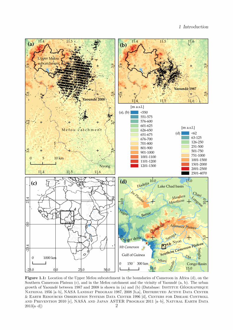
Figure 1.1: Location of the Upper Mefou subcatchment in the boundaries of Cameroon in Africa (d), on theSouthern Cameroon Plateau (c), and in the Mefou catchment and the vicinity of Yaoundé (a, b). The urbangrowth of Yaoundé between 1987 and 2008 is shown in (a) and (b) (Database: Institue GéographiqueNational 1956 [a–b], NASA Landsat Program 1987, 2008 [b,a], Distributed Active Data Center& Earth Resources Observation Systems Data Center 1996 [d], Centers for Disease Controlland Prevention 2010 [c], NASA and Japan ASTER Program 2011 [a–b], Natural Earth Data2013[a–d]) 2
1 Introduction
drastic increase of Yaoundé’s population and urban area (for the population development ofcolonial Yaoundé, cf. Franqueville 1979); also for Cameroon’s largest city and economiccenter Duala, a fast growing population is reported (Hanna & Hanna 2009). As statedbefore, urban growth and deforestation have an influence on soil erosion—the same goes forthe Southern Cameroon Plateau.The study at hand takes up these issues and focuses on the assessment of the actual, potentialand future soil erosion risk in the Upper Mefou subcatchment, a catchment located in theintermediate vicinity of periurban Yaoundé (Figure 1.1a,b).
Soil erosion modelling
Soil erosion modelling is a common approach for soil erosion risk assessment, besides fieldmapping of erosion damages, analysis of sediments and suspended load, exposed-root surveys,factor scoring or participative/expert approaches. In the humid tropics, soil erosion modellingis problematic: Most of the erosion models were developed and calibrated in a differentclimatic, topographic and geological setting, where cultivation is completely different. Someof the models were applied in the humid tropics, but the databases and validations—especiallyof empirical models—are not adapted to that region.In the study at hand, RUSLE3D, a three-dimensional modification of the Revisited UniversalSoil Loss Equation (RUSLE), and the topographic deposition routine of USPED (Unit StreamPower Erosion Deposition) will be applied in the Upper Mefou subcatchment. Althoughthere are a lot of restrictions and limitations of the USLE-family models, there are somegood reasons to use the RUSLE3D for soil erosion risk assessment in the Upper Mefousubcatchment: (i) The application of USLE-family models is discussed for the humid tropicsand some authors successfully applied the model in western Africa (Millward & Mersey1999; Angima et al. 2003 or Roose 1977; Mati & Veihe 2001); (ii) thus, the model outputsand the values of input parameters can be compared with other studies and put in context.(iii) A number of attempts were made to adapt the input factor to the humid tropics (rainfallerosivity: i. a. Salako et al. 1991; Bresch 1993; Yu 1998; Salako 2008; Salako 2010;Diodato et al. 2013; erodibility: i. a. Roose 1977; Vanelslande et al. 1987; Roose &Sarrailh 1989; Nill 1993; crop management and cover: i. a. Roose 1977; El-Swaifyet al. 1982; Nill 1993; Nill et al. 1996 ); (iv) USLE-family models can easily be used forsimulations. (v) empirical models—like the USLE— are recommended for the catchmentscale, whereas conceptual or physical models are recommended for a smaller scale; empiricalmodels are suitable for long term analysis (Volk et al. 2010); (vi) therefore, the erosion riskis well sufficiently assessed with an empirical model. (vii) Although the predicted soil loss
3
1 Introduction
values have to be analysed critically, RUSLE3D is suitable as a semi-quantitative tool for riskassessment (Vrieling et al. 2008); (viii) the model is suitable within the wider framework ofthe study, as it is important to use simple, low input models which can easily be implementedin widespread open source software. (ix) The easily understandable input parameters areappropriate for capacity building purposes.
Integrated Watershed Management
The study at hand is part of the international research and development project Enhancingcollaborative research and development capacities of German and Sub-Saharan African partnerson Integrated Watershed Management (IWM). The project focuses on the communicationgap between scientists, decision makers and local population with the goal to bridge thesegaps. In three partner countries (Cameroon, Kenya and South Africa) joint research of localand German students in so called “living laboratories” is conducted, where awareness raisingtakes place during field work. In addition, activities in the living laboratories should be usedfor teaching purposes and stakeholder workshops.The living laboratory in Cameroon is the Upper Mefou subcatchment, i. e., the headwaters ofthe Mefou River, a tributary of the Nyong River. The watershed is located in the humidtropics of the South Cameroon Plateau and comprises a periurban part of Yaoundé and arural part, which is covered with typical Guineo–Congolaise type rainforest and used forshifting cultivation, forestry and cash crop production. One feature of the catchment is theMefou Reservoir (Barrage du Mopfou), which is an important component of the urban watersupply of Yaoundé.Integrated Watershed Management (IWM) is a holistic approach: The management ofall resources in a watershed is included, both biophysical resources (water, soil, biomass)and human resources, which include the sociocultural, economic, political and institutionalconsiderations in a watershed (Easter & Hufschmidt 1985). IWM is a research anda management approach. Besides scientists, also non-governmental organizations, (local)administration and stakeholders participate (Förch & Schütt 2005). The IWM-processincludes a planning and an implementation step, i. e. the formation and design of activities andthe installation, operation, maintenance and evaluation of measures (Easter & Hufschmidt1985). The role of scientists is not at least the collection and analysis of basis informationand the identification of key problems. A watershed is the spatial basis of IWM. It is atopographic defined land area, which drains to one point of a stream (Ffolliott 2011). Theconcept is therefore based on natural boundaries. Administrative boundaries are neverthelessimportant, due to the fact that different institutional settings may exist in a watershed that
4
1 Introduction
is located in different administrative units (Easter & Hufschmidt 1985). The interactionbetween upland and downstream areas is an important part of IWM. As a watershed is not acontainer, off-site effects should not be ignored. The IWM-approach and soil erosion studiesare methodological linked. The watershed is a functional unit with physical relationships,which are also important for soil erosion, as it is the case for upstream–downstream linkages(Dixon & Easter 1991). Various studies combine erosion assessment and IWM, such asHoare (1991) in Thailand, Briones (1991) in a Philipine watershed or Beck et al. (2004)in Ethiopia. Soil erosion is apprised to be one of the major biophysical aspects in a watershedand linked to human disturbance (Hamilton & Pearce 1991). Erosion is one of the“challenges faced” in IWM (Gregersen et al. 2007: p. 6).During an initial implementation workshop of the IWM-project in Cameroon and during astakeholder workshop in the Upper Mefou subcatchment in November 2013 (Becker et al.2013) the problem of soil erosion was addressed, not least because of the potential siltationof the Mefou Reservoir and an impact on the quality of the water supply for Yaoundé.
Objectives
As one of the tasks of IWM is to “develop a rapid diagnostic methodology to access thecondition of watersheds and to formulate and evaluate possible course of actions” (Easter& Hufschmidt 1985: p. 2), the objectives of the study on hand are:
1. to assess the soil erosion risk in the study area,2. to evaluate the possible impacts of land use and land cover changes on the soil erosion
risk and3. to evaluate the applied methods to find out if they are suitable for the context of the
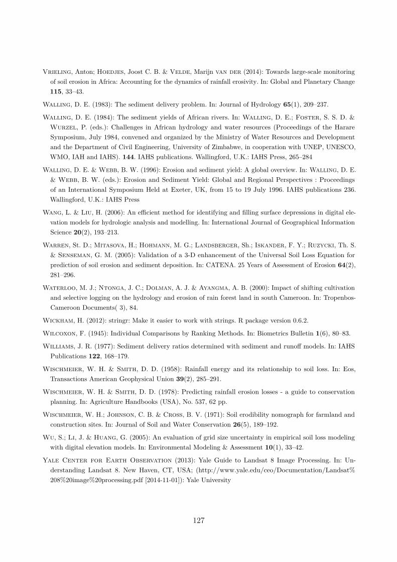
study catchment.Objective 1 includes the evaluation of the erosion determining factors as they are includedin the RUSLE3D-model: Rainfall erosivity, soil erodibility, topographic potential of erosion,land cover and crop management and conservation measures. The topographic potentialof deposition are calculated separately—based on a topographic erosion/deposition indexderived from USPED (Mitasova et al. 1996; Hofierka et al. 2009).In various studies, soil erosion risk assessment includes the calculation of the actual and longterm soil erosion risk—often with a USLE approach—and the future soil erosion risk (cf.Prasuhn et al. 2013). Therefore, Objective 2 comprises the development of potential landuse and land cover change scenarios and the assessment of the expected effect on soil erosion.In addition to actual and future soil loss, potential soil loss is calculated, which covers ina broadly sense the natural sphere of soil erosion (the physical parameters rainfall, relief,
5
1 Introduction
soils), but not the human activities (land use and land cover, soil conservation measures). Asthe term risk includes the “exposure to . . . the possibility of . . . unwelcome circumstances”(Oxford English Dictionary), soil erosion is not only estimated, but assessed in comparisonwith tolerable soil loss. As the USLE-familiy models are not developed for the characteristicof the study region, different approaches are used to calculate the input parameters of theRUSLE3D to show the problematic of the adaption of an approach to other conditions. Themain aim of Objective 3 is therefore to consider the applicability of the RUSLE3D on theSouthern Cameroon Plateau.Objective 3 should also be pursued by comparing the values of all input factors of RUSLE3Dwith the results of other studies in a similar context. This should firstly give informationon the plausibility of the modelled erosion values (fit-to-reality) and simultaneously allowto estimate if values are high or low. In addition the model results will be evaluated bycomparing soil erosion values and sediment yield data obtained by a reservoir sedimentationsurvey. A sensitivity analysis of the USLE-input parameters will be conducted to show theweighting of the input factors of the model (and a potential delicateness of errors).
6
2 State of the Art
2.1 Soil erosion
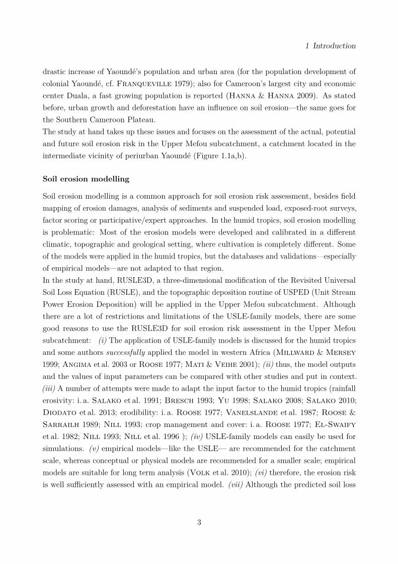
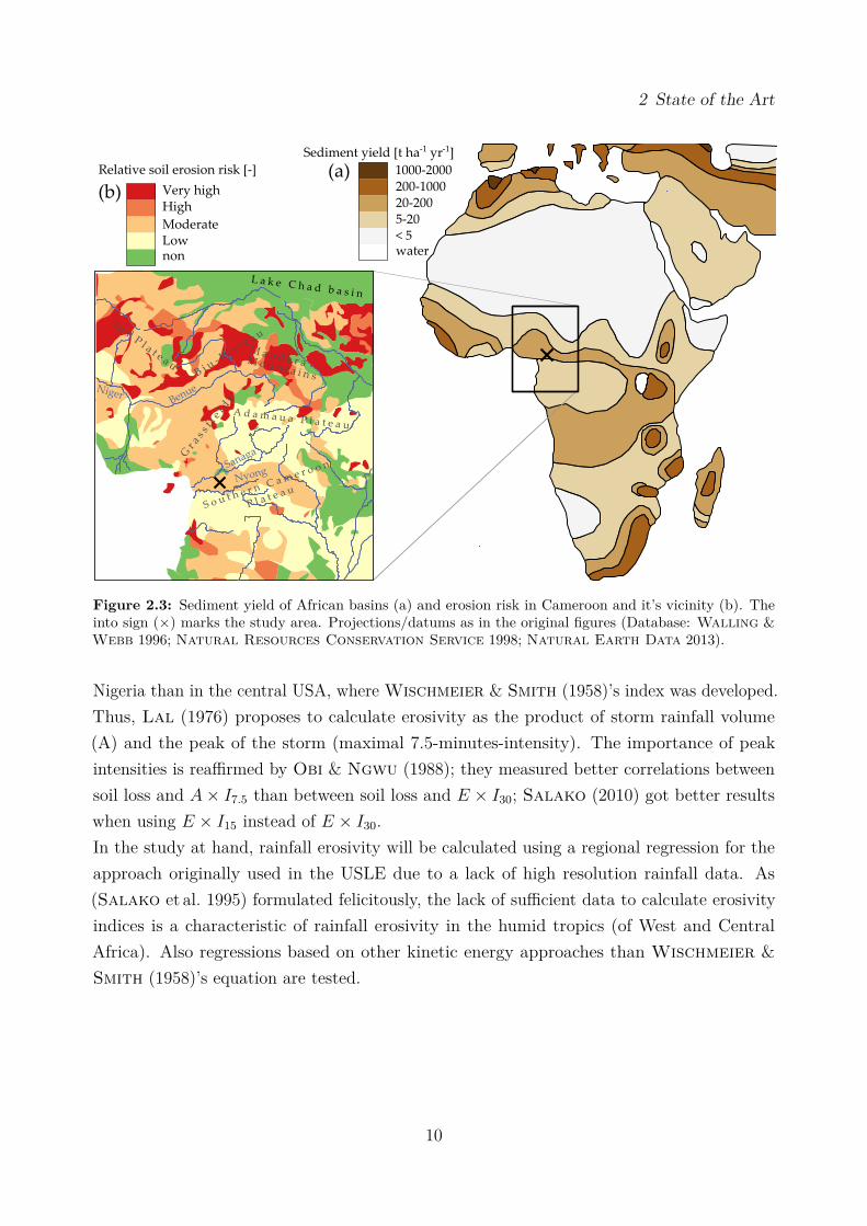
Erosion is a function of various parameters and controlled by the energy force of rainfall(erosivity) and the relief, the resistability of soil particles to detachment and transport(erodibility) and the protective function of vegetation cover and soil conservation measures(Morgan 2009; Figure 2.1). Eroded soil is deposited in the catchment on fields, on foot slopes,in floodplains, in channels or other sinks and depressions (Fryirs 2013). The sediment notstored in the catchment is the sediment yield (Figure 2.1). Topography and rainfall erosivityare mainly natural forces. The erodibility of a soil is first and foremost a natural characteristicbut is also influenced by human impact such as fertilization or overuse. (Ground) cover iseither natural or, as it is often the case, influenced by human land use.The energy of the forces varies between different landscapes around the world. Erosivity anderodibility in the humid tropics are quite different from the temperate or more dry regions;they are determined by different parameters. Therefore, the extent of soil erosion is specific.In tropical Africa, rainfall erosivity has the lowest variability between different places (factor:14–20, Nill 1997). Also the soil loss variability when applying different soil conservationmeasures is relatively low. The maximal factor is 1 representing a lack of conservationmeasures; the minimal factor is 1/25 (hillslope terracing). Both, erodibility and topographyvary on a wide scale in the tropics. Some soils have a 580-times higher erodibility value(determined with the USLE) than the least erodible soils. The impact of topography can bevery low on flat, short slopes and up to 640 times higher on steep, long slopes (Nill 1997).This variability is not specific for the tropics, as in a lot of other regions, both flat and steepslopes are located. According to Nill (1997), the crop cover was the highest relative distancebetween low and high values. For example, he reports an USLE-C-factor of 0.0002 for “densetropical forest or 100% mulch cover” and a value of 0.58 for plowed upland rice. Land useand land cover differs within small catchments, where soil erodibility and especially rainfallerosivity are relatively constant.For most of the Southern Cameroon Plateau a “medium” (Natural Resources Conser-vation Service 1998) soil loss amount is expected (Figure 2.3a). The annual sedimentyields in the region is estimated at 20–200 t ha−1 (Walling & Webb 1996). In comparisonto the Guinea savanna in the north and the Equatorial Forest in the south (especially in theCongo basin), the sediment yield is relatively high (Figure 2.3b).
2 State of the Art
Energy force
Protection
Resistance
Rainfall
Topography
Cover
Soil erodibility
Ground cover
Conservation measures
N a t u r a l s p h e r e H u m a n s p h e r e+= SOIL EROSION DEPOSITION SEDIMENT YIELD
Figure 2.1: The human and natural sphere of soil erosion.
Rainfall erosivity is relatively high in the humid tropics, whereas soil erodibility is expectedto be low (Figure 2.2, cf. Ambassa-Kiki & Nill 1999). Supposing a natural vegetationcover, sediment yield is low in the humid tropics (Figure 2.2, cf. Langbein & Schumm1958); due to land use and deforestation, the natural vegetation cover on the SouthernCameroon Plateau is disturbed and sediment yields might be much higher. Although theSouthern Cameroon Plateau is characterized by a moderate relief, the relief in the UpperMefou subcatchment is relatively high and steep; the Yaoundé massif is the highest massif onthe Plateau (Olivry 1986).
2.1.1 Erosivity of tropical rainfall
Rainfall erosivity in the tropics—and especially in the humid tropcis—is characterized by highamounts and high intensities and therefore a high kinetic energy (Vrieling et al. 2010). Incomparison to the other forces and parameters of soil loss, the erosive force is the strongest inthe humid tropics (Ambassa-Kiki & Nill 1999; Vrieling et al. 2010). Erosivity per rainfallamount is lower in the semi-arid tropics than in the humid tropics (Nill 1998). Besidesthe high annual rainfall totals (more than 10 000mm at Mount Cameroon), the drop-sizedistribution of tropical rains is often reported to be one reason for the high kinetic energy ofstorms. The energy of tropical large drops is higher due to a higher terminal velocity (VanDijk et al. 2002). In addition, larger drops occur more often during high intensity storms(Salako et al. 1995).The positive effect of wind on erosivity of tropical storm is often reported (Arnoldus 1980;Nill 1997), but not true for all locations (Salako et al. 1995). This emphasizes the highvariability of erosivity within the tropics.
8
2 State of the Art
Rel
ativ
e,an
nu
al,s
edim
ent,
yie
ld
Precipitation,[mm]
1000500 2000
approximated,relation
measured,relation,
So
il,e
rod
ibil
ity
,K,[
SI]
Rainfall,erosivity,R,[SI]
10,000 15,000 20,0005,000
0.00
10.
002
0.00
30.
004
humidmountainoussemi-humiddrytropical
Climate
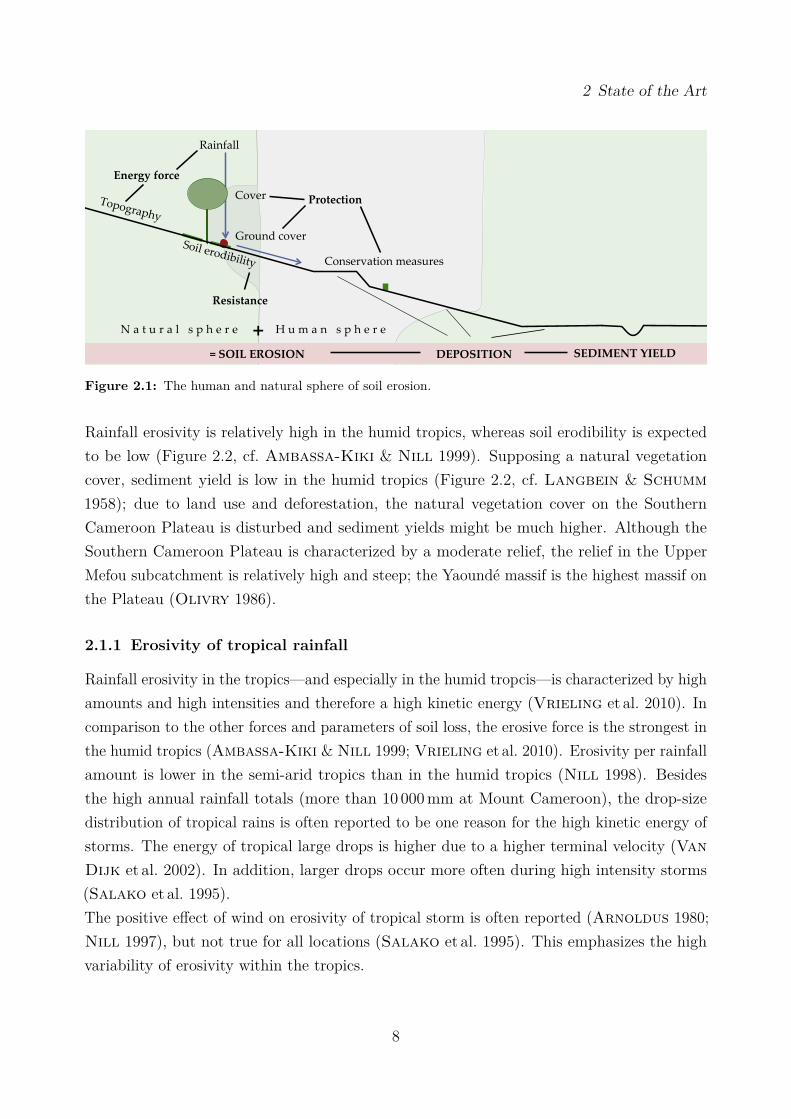
Figure 2.2: (a) Soil erodibility in relation to rainfall erosivity and precipitation regime (Roose & Sarrailh1989, dots, and Nill 1998, line) and (b) sediment yield as a function of precipitation obtained from reservoirdata from the US (Langbein & Schumm 1958); both USLE-factors in metric units (see Section 4.1). InLangbein & Schumm (1958)’s relation, the variation in annual sediment yield with precipitation is tracedto a change in natural vegetation cover. The annual precipitation at Nkolbisson, close to the Upper Mefousubcatchment, totals ca. 1600mm, what corresponds to an roughly approximated rainfall erosivity R-value of12100–13400 (Roose 1977).
55% of the rainfall events are short and characterized by an early intensity peak; 45% of therainfall events are long, but intensities are low (Salako et al. 1995; cf. Obi & Salako 1995).Both types have a high erosivity, one because of intensity, one because of volume (Salakoet al. 1995).The spatial distribution of erosivity within tropical West and Central Africa varies withaltitude, distance to coast and latitude. In the west, heavy rainstorms are more pronouncedthan in the East (Diodato et al. 2013). The highest erosivity values in Africa were foundon the western coasts of West and Central Africa (Vrieling et al. 2010), what might beexplained by wind systems. Erosivity per rainfall amount is generally higher at the coasts,whereas it is lower in the inland and even lower in the highlands, because mean drop sizesand intensities are lower in highlands (Nill 1997). For Cameroon, Nill (1997) reports arainfall–erosivity ratio of 10:124 for coastal stations, 10:111 for inland stations and 10:82 forhighland stations.
Erosivity of tropical rains in the USLE
In the USLE and it’s revision (Wischmeier & Smith 1978; Renard et al. 1997) rainfallerosivity is the product of the kinetic energy (E) of a storm and the maximal 30-minute-intensity (I30) (Wischmeier & Smith 1958). Lal (1976) investigated rainfall and soil lossnear Ibadan, Nigeria, and concludes that this relationship underestimates erosivity of tropicalrain. The slope of the regression between kinetic energy and rainfall amount is steeper in
9
2 State of the Art
ka[kb[
<s55-2020-200200-10001000-2000
water
ModerateLownon
HighVeryshigh
BenueNiger
Sanaga
Nyong
J o s s P l a t e a u
Gr a
s s f ie
l ds
M a n d a r a sM o u n t a i n s
A d a m a u a s P l a t e a u
B i u - P l a t e a u
S o u t h e r n s C a m e r o o n s
P l a t e a u
L a k e s C h a d s b a s i n
Sedimentsyields[tsha-1syr-1]
Relativessoilserosionsrisks[-]
Figure 2.3: Sediment yield of African basins (a) and erosion risk in Cameroon and it’s vicinity (b). Theinto sign (×) marks the study area. Projections/datums as in the original figures (Database: Walling &Webb 1996; Natural Resources Conservation Service 1998; Natural Earth Data 2013).
Nigeria than in the central USA, where Wischmeier & Smith (1958)’s index was developed.Thus, Lal (1976) proposes to calculate erosivity as the product of storm rainfall volume(A) and the peak of the storm (maximal 7.5-minutes-intensity). The importance of peakintensities is reaffirmed by Obi & Ngwu (1988); they measured better correlations betweensoil loss and A× I7.5 than between soil loss and E × I30; Salako (2010) got better resultswhen using E × I15 instead of E × I30.In the study at hand, rainfall erosivity will be calculated using a regional regression for theapproach originally used in the USLE due to a lack of high resolution rainfall data. As(Salako et al. 1995) formulated felicitously, the lack of sufficient data to calculate erosivityindices is a characteristic of rainfall erosivity in the humid tropics (of West and CentralAfrica). Also regressions based on other kinetic energy approaches than Wischmeier &Smith (1958)’s equation are tested.
10
2 State of the Art
2.1.2 Erodibility of tropical soils
On of the most important and most widely discussed factors determining erosion is theconcept of erodibility. Following the definition of Morgan (2009: p. 50) erodibility isthe “resistance of the soil to both detachment and transport”. Three assumptions are metas a common understanding of the concept: First, soil erodibility is valid for all watererosion processes; second, soil erodibility is a function of a limited number of measurablesoil properties; third, soil erodibility is constant for a specific period of time (Bryan et al.1989). Although topography and location parameters (e. g. slope) or the degree of physicalstress (e. g. tillage) influence soil erodibility, soil properties are deemed primary important(Bryan et al. 1989; Bryan 2000; Morgan 2009). These properties are texture, sear strength,infiltration capacity and organic and chemical components (binding agents). Sand and clayare more resistant to detachment and transport than silt; sand because more kinetic energyof overland flow is necessary to transport particles, clay because they are bound in complexes.Soils with a content of the silt fraction between 40 and 60% are most erodible (Morgan2009).Apparent particles but coarse sand are often aggregated. Aggregates are either formed byphysical stress or by binding agents (Bryan 2000). Macroaggregates are less susceptible todetachment and transport. Soil organic matter is the strongest binding agent in most soils.While humid acids, microbila debris, polysaccharides or mucilages stabilized microaggregates(< 250mm), plant debris, roots, hyphae, plant nuclei bind macroaggregates (> 250mm)(Edwards & Bremner 1967; Oades & Waters 1991; Bryan 2000). The type of organicmaterial is also important for it’s influence on erodibility, as litter and large plant remains donot influence aggregate stability (Morgan 2009). Also clay—depending on the mineralogy ofthe clay minerals—is a binding agent (clay flocs); the sodium adsorption ratio is responsiblefor differences in aggregate stability. The third type of binding agents are polyvalent metals(Edwards & Bremner 1967), often in a complex with clay and organic matter. Fortropical soils, they are more important than organic bonds (Oades & Waters 1991).Igwe et al. (1995) show that soil samples treated with sodium dithionite-citrate-bicarbonateto dissolve ferric oxides and aluminium oxides have higher clay contents; Mbagwu &Schwertmann (2006) gained similar results and measured an only slightly higher claycontent after the removing of organic matter with hydrogen peroxide. However, Barthèset al. (2008) measured a dissolution of water-stable aggregates correlated to organic mattercontent, but concluded that the correlation with sesquioxides for tropical soils is muchhigher and the relationship between organic matter content and aggregates depends onthese sesquioxides. Besides aggregate stability, also the size of aggregates, their shape and
11
2 State of the Art
their size homogenity is of importance. Macro- or microaggreagetes are bound by differentagents, which are characterized by a different susceptibility to dissolution. Size homogentiy ofaggregates affects pore volume and therefore infiltration capacity of soils. Infiltration capacitydetermines erodibility due to the fact that high infiltration capacity limits the proportionof overland low (Morgan 2009). Shear strength expresses the resistance of a soil to theenergy of flowing water (and gravitation). Together with the surface roughness, which bothdepend on soil texture, pore volume, shear strength and infiltration capacity are the mainhydrological parameters of soil erodibility. Antecedent water content is as much relevant:Overland flow is more probable on a wet soil; wet aggregates are less stable and surfacesealing might appear (Bryan 2000; Morgan 2009). Taking this parameters into account, itseems to be evident that erodibiltiy is very variable in space and time.As it is mentioned by El-Swaify et al. (1982) and Nill (1998) the variability of the erodibilityof tropical soils is extraordinary high; soils of the same order have different soil erodibility.The values range from 0.06 to 0.48 (El-Swaify et al. 1982) or from 0.0006 to 0.35 with amean of 0.08 ton acre h 100−1 acre−1 ft−1 tonf−1 in−1 (Nill 1998). In general, the erodibilityof tropical soils is classified as low due to a high content of weathering-resistant sand (highinfiltration capacity) organometallic complexes and Kaolinite as a binding agent. The siltfraction is often weathered.
Erodibility estimation
To be included in a soil erosion model, erodibility has to be measured or approximated;either by measuring soil loss under controlled conditions or by an index taking various soilproperties into consideration (Bryan 1968; Morgan 2009). One index is Middleton’sdispersion index, which is the ratio of the fraction of non-dispersed silt and clay and thefraction of dispersed silt and clay. Other early indices are based on the clay ratio (Bouyoucous’index), the amount, size and stability of aggregates (Gerdel’s index), organic matter (Peeleet al.’s index) or a complex interaction of grain size, permeability, absorption and dispersion(Bayer’s index; for an overview of the history of indices and formulas Bryan 1968; Morgan2009). In the USLE, erodibility is expressed by the K-factor, which is based on a unit plotdatabase. A nomograph was developed to estimate the K-factor based on organic mattercontent, grain size, permeability and soil structure. Due to the fact that the database of thenomograph is only valid for some parts of the US, the application of the K-factor for tropicalconditions is under discussion. Roose & Sarrailh (1989) found a good correlation betweennomograph approximations and measured K values, while others voiced criticism and foundlower correlations. Among others, Roth et al. (1974) developed a nomograph which is well
12
2 State of the Art
adapted to tropical conditions, taking aluminium and ferric oxide as well as silicon dioxideinto account. Nill (1993) developed a scheme to convert nomograph values into tropicalK-values. This scheme is used in the study at hand.
2.2 Soil erosion modelling
As models in general, erosion models are simplified depicted realities of a specific part ofthe landscape (Bork & Schröder 1996). Using parameters, factors, their constellationand interaction, erosion models are a representation of real erosion processes. Soil erosionmodels are an academic and land stewardship approach to cope with soil erosion. Amongother approaches—e. g. measurement, mapping and sediment sampling—soil erosion modelshave been developed within the last one hundred years. Especially after the Dust Bowlin the United States (1934–1940), attempts were made to focus on erosion models for soilconservation. As the number of models is huge and a lot of reviews and state-of-the-artdescriptions exist (Bork & Schröder 1996; Merritt et al. 2003; Morgan & Nearing2010; Borrelli 2011; Schmengler 2011) only a general view of different types of modelsis given in the following.Models are either empirical, physical or conceptual. Empirical models are based on empiricalmeasurements on plots or in catchments. The results are used to calculate regressions betweendifferent parameters. The problem of these models is that values measured at one location aredifficult to use in other climates, land use schemes, soils and topographic conditions. Physicalmodels in contrast are based on the principal laws of physics. Often physical models requiremore input than empirical models. Conceptual models are based on flows and storage in acatchment; they only generally describe the processes in a catchment (Merritt et al. 2003).All these types of models can be both, deterministic or stochastic. Deterministic modelsare based on a defined input value of a parameter, whereas stochastic models are based onprobability distributions of the input parameters. The temporal representation of modelsincludes temporally static input parameters or time-depended input parameters. Erosionmodels are event-based or continuous. Continuous models in turn can be based on meanvalues over a specific time period or represent the variability of processes over a longer period(Bork & Schröder 1996). The spatial representation of erosion models ranges from plotscale to basin scale (cf. Renschler & Harbor 2002). This is especially important due tothe fact that the contribution of different types of erosion (interrill, rill or gully erosion) tototal soil loss depends on scale (Evans & Brazier 2005). Also the proportion of erosion anddeposition varies with scale. On a small hillslope, deposition and sediment storage is much
13
2 State of the Art
smaller than in a catchment (De Vente et al. 2008). Thus, hillslope erosion models existas well as field, small catchment and catchment scale models (Merritt et al. 2003). Theinput parameters vary over the area of investigation when applying distributed models. Inputparameters are constant over the entire area in lumped models. The spacial discretizationdepends on whether models are based on homogeneous compartments of the landscape(subcatchments, hydrological response units), homogeneous portions of a slop in the directionof flow or regular portions of the landscape (grid cells; Bork & Schröder 1996). Functionalrelationships—especially important concerning the flow direction of water—are considered inthe first two approaches, but less integrated in the latter one.
The USLE-family
An empirical, deterministic and continuous erosion model is the Universal Soil Loss Equation(USLE). The USLE and its modifications are one of the most used erosion models worldwide. The USLE was developed in the United States in the late 1950s. First applicationstook place in the early 1960s in the Midwest (Renard et al. 1991); the first version ispublished in the USDA Agricultural Handbook 282. A second version of the Handbook waspublished in 1978 (USDA Agricultural Handbook 537, Wischmeier & Smith 1978) and isthe standard reference to the model. A revisited USLE (RUSLE) was first published in 1991and is described in the USDA Agricultural Handbook 703 (Renard et al. 1997). Furtherdevelopments are implemented in a more computerized version (RUSLE2, Foster et al. 2000;USDA Agricultural Research Service 2013). A 3-dimensional version of the RUSLEwas developed for GIS applications and convergent flow on catchment scale (RUSLE3D)and erosion and deposition modelling (USPED, Mitasova et al. 1996). Other models weredeveloped on the basis of the USLE, e. g. the sediment delivery model MUSLE (Williams1977) or the USLE-M (Kinnell & Risse 1998), which explicitly includes runoff.The original USLE is based on a huge database of values from a bare standard “Wischmeier”-plot with a length of 72.6 ft (22.13m), a wide of 6 ft (1.83m) and a slope of 9%, where soilloss is a linear function of erosivity and erodibility (cf. Wischmeier & Smith 1978).The results can be used to calculate soil loss on plots different from the standard plot. Factorsare used to get the soil loss for other land cover, topography or conservation measures. Theprocedures to calculate the factors are described in the USLE manual (Wischmeier &Smith 1978).The Revisited USLE includes some major improvements; all factors are calculated differently.A new rainfall–erosivity term was adapted which is based on a larger data set than the termused in the USLE. In addition, snow is included in the RUSLE (Renard et al. 1991; Bork
14
2 State of the Art
& Schröder 1996). The parameter of the slope length was modified and is now calculatedas a ratio of rill to interrill-erosion. While in the USLE C- and K-values are calculated onthe temporal basis of crop stages, they are calculated for half month intervals in the RUSLE.In addition, the C-factor in the RUSLE is based on several subfactors and is a function ofmulch or ground cover, crop residues, roots and a subsurface cover (Renard et al. 1991).The USLE’s C-factor is based on the weighted average soil loss ratio of a plot with the landcover under investigation and the standard plot. A critical slope length for conservationmeasures is newly integrated in the RUSLE’s P-factor (cf. Bork & Schröder 1996). Inthe RUSLE3D and the USPED model, slope length is replaced by upslope area, which takesconvergent flow into account. In addition, the Unit Stream Power Theory (Moore & Burch1986b) is used in the USPED model to calculate erosion and deposition (Mitasova et al.1996). The USLE assumes erosion on the entire plot/catchment.
USLE limitations
Although the USLE-family models received wide attention and are applied frequently, thereis a great deal of criticism. Some of the points commented are improved in the revisitedversion(s), but are nonetheless important to consider:
• the equation is based on mean values over a longer period. Thus, event-based erosion isnot calculated with the USLE (Merritt et al. 2003), although single events contributeto a high proportion to total soil loss.
• Although gully erosion or mass movements are largely responsible for total soil loss,they are not calculated with the USLE (Merritt et al. 2003).
• In the USLE—and most of its modifications and revisions but the USLE-M (Kinnell& Risse 1998)—runoff is not considered explicitly.
• The calculation of rainfall erosivity is based on a limited database; only drop sizemeasurements from 1943 in Washington, D.C., and velocity measurements from 1949were included (Bork & Schröder 1996);
• soil erodibility as in the USLE is only valid for silt contents less than 70%, which makesit difficult to apply the equation in loess soils. In addition, the erodibility increases withincreasing aggregate sizes, which is contrary to the actual process (Bork & Schröder1996);
• as it is shown by Dikau (1986), the equation is very sensitive to slope length andinaccuracies are very good correlated to slope length variations;
15
2 State of the Art
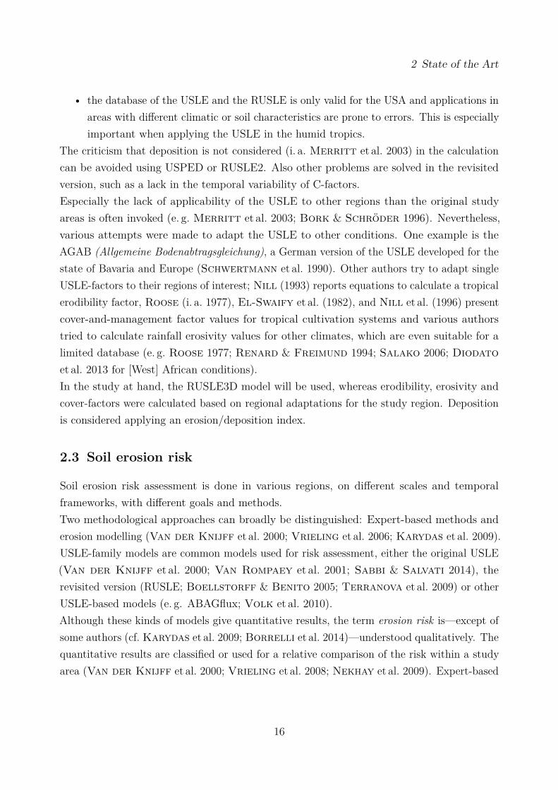
• the database of the USLE and the RUSLE is only valid for the USA and applications inareas with different climatic or soil characteristics are prone to errors. This is especiallyimportant when applying the USLE in the humid tropics.
The criticism that deposition is not considered (i. a. Merritt et al. 2003) in the calculationcan be avoided using USPED or RUSLE2. Also other problems are solved in the revisitedversion, such as a lack in the temporal variability of C-factors.Especially the lack of applicability of the USLE to other regions than the original studyareas is often invoked (e. g. Merritt et al. 2003; Bork & Schröder 1996). Nevertheless,various attempts were made to adapt the USLE to other conditions. One example is theAGAB (Allgemeine Bodenabtragsgleichung), a German version of the USLE developed for thestate of Bavaria and Europe (Schwertmann et al. 1990). Other authors try to adapt singleUSLE-factors to their regions of interest; Nill (1993) reports equations to calculate a tropicalerodibility factor, Roose (i. a. 1977), El-Swaify et al. (1982), and Nill et al. (1996) presentcover-and-management factor values for tropical cultivation systems and various authorstried to calculate rainfall erosivity values for other climates, which are even suitable for alimited database (e. g. Roose 1977; Renard & Freimund 1994; Salako 2006; Diodatoet al. 2013 for [West] African conditions).In the study at hand, the RUSLE3D model will be used, whereas erodibility, erosivity andcover-factors were calculated based on regional adaptations for the study region. Depositionis considered applying an erosion/deposition index.
2.3 Soil erosion risk
Soil erosion risk assessment is done in various regions, on different scales and temporalframeworks, with different goals and methods.Two methodological approaches can broadly be distinguished: Expert-based methods anderosion modelling (Van der Knijff et al. 2000; Vrieling et al. 2006; Karydas et al. 2009).USLE-family models are common models used for risk assessment, either the original USLE(Van der Knijff et al. 2000; Van Rompaey et al. 2001; Sabbi & Salvati 2014), therevisited version (RUSLE; Boellstorff & Benito 2005; Terranova et al. 2009) or otherUSLE-based models (e. g. ABAGflux; Volk et al. 2010).Although these kinds of models give quantitative results, the term erosion risk is—except ofsome authors (cf. Karydas et al. 2009; Borrelli et al. 2014)—understood qualitatively. Thequantitative results are classified or used for a relative comparison of the risk within a studyarea (Van der Knijff et al. 2000; Vrieling et al. 2008; Nekhay et al. 2009). Expert-based
16
2 State of the Art
methods generally only give relative results (e. g. Le Bissonnais et al. 2002; Bou Kheiret al. 2006; Vrieling et al. 2006). The results of an erosion risk assessment is consistentlya relative risk map of “hotspots” or priory areas, which show the spatial distribution ofthe erosion risk (Nigel & Rughooputh 2010; Volk et al. 2010). The goal of this riskmapping is risk management and erosion control—i. e. planning and implementation of soilconservation measurements (Vrieling et al. 2006)—, the identification of priority areas(Nigel & Rughooputh 2010) or policy development and decision-making (Le Bissonnaiset al. 2002; Boellstorff & Benito 2005; Mutekanga et al. 2010).Concerning these goals, the spatial scale of erosion risk assessment is important. On theEuropean and national scale, policy development (set-aside scenarios or agricultural supportplanning) is important, the planning of conservation measures is important on local scale.Especially the risk assessment on continental scale emphasize the relative character of erosionrisk, as it is difficult to model exact values on that scale (Vrieling et al. 2008). The areasof erosion risk studies range from small municipalities (Karydas et al. 2009) to nationalterritories (Le Bissonnais et al. 2002; Sabbi & Salvati 2014) or even the European Union(Van der Knijff et al. 2000) on the level of political hierarchies and from small watersheds(Vrieling et al. 2006; Borrelli & Schütt 2014) to large river basins (Zhang et al. 2010).Other studies assess erosion risk of regions or islands (Boellstorff & Benito 2005; BouKheir et al. 2006 or Nigel & Rughooputh 2010).Soil erosion risk is often seen as the interaction of different factors, which are either specificfor an area or human-induced. Therefore, there are other terms related to erosion risk. Nigel& Rughooputh (2010) define erosion risk as the interaction of erosion susceptibility (ofthe topography) and sensitivity (of the land cover) in combination with rainfall erosivity.Other authors use susceptibility more or less synonym to risk (Borrelli & Schütt 2014)or as an inherent character of a landscape (soil, topography, climate; Giordano n. d.). Theinherent susceptibility is expressed in many studies by the potential erosion of an area—ora “worst case scenario” (Renschler et al. 1999)—whereas the present land use and landcover determines the actual (or current) erosion risk (Mutekanga et al. 2010; Zhang et al.2010; Sabbi & Salvati 2014). This distinction is used by some authors to give erosion riska temporal dimension: The change of land use and land cover is used to calculate eitherhistorical (Mutekanga et al. 2010) or future erosion risk (Prasuhn et al. 2013). Also thepossible reduction of soil erosion risk is estimated (Karydas et al. 2009) or the erosion riskof environmental changes is evaluated (Zhang et al. 2010).Risk is interpreted in most studies as a relative term of assessed erosion in a study. Onlysome authors set erosion risk in context to the economic or ecological consequences of soil loss
17
2 State of the Art
(e. .g. costs of erosion or tolerable soil loss); e. g. Renschler et al. (1999) and Boellstorff& Benito (2005) or Giordano (n. d.) can be mentioned here. As risk is seen as a relativevalue, the results are not always validated, an exception being Le Bissonnais et al. (2002)or Borrelli et al. (2014).
18
3 Study areaThe Upper Mefou subcatchment is located in the Région du Centre (Central province) in theRepublic of Cameroon. The country belongs either to the West African or to the CentralAfrican subregion of the continent—depending on definition. While the small southeasternpart of the catchment is located in the Département du Mfoundi (Mfoundi division), alarger portion is within the boundaries of Lekié division. The catchment is located in fourarrondissements (subdivisions): Yaoundé VII, Yaoundé II, Lobo and Okola. Most of thevillages are located in Okola. Beyond this administrative structure, there is also a system ofheritage chiefdoms (traditional authorities, French: chefferies traditionnelles). The villages ofthe catchment are organized in this system and it’s different hierarchies, which comprises achef de troisième degré (chief of a village) and a chef de groupement and a chef supérieur. Theirrole is important concerning land ownership and land use (for the northwest of Cameroon:Diduk 1992).Within the framework of the Integrated Watershed Management project a bridge in Nkolbisson(3◦ 52′ 20.6′′N, 11◦ 27′ 02.2′′ E) marks the outlet of the project’s catchment. The outlet islocated between the confluence of the Mefou River and the Afeumev/Afemé River and themouth of the Abiergue River to the Mefou. The catchment area of the Upper Mefou is97 km2; the altitude ranges from 701m at the outlet to 1225m a. s. l. at the highest point inthe Yaoundé massif (Odou summit).The Mefou River is a right tributary of the Nyong, which forms one of the major river basinsin Cameroon and drains to the Bight of Bonny (Gulf of Guinea). The confluence is located10 km east of Mbalmayo (river-kilometre 345). The catchment area of the Mefou is about840 km2 (Olivry 1986). The northwestern divide of the Upper Mefou subcatchment is alsothe major Nyong–Sanaga divide.Upper Mefou discharge-data are not available at the moment, as it is the case for data ofthe Mefou Reservoir. A gauge close to the outlet is out of operation and in a dilapidatedcondition. Discharge was recorded in the past (Lefèvre 1966), but data are not available atthe present. Discharge of the Mefou is recorded at Etoa (235 km2, 672m a. s. l., observationperiod: 1966–1977) and Nsimalen (425 km2, 650m a. s. l., 1962–1977). The mean annualdischarge of the Mefou at Etoa is 3.3 and 6.1m3 s−1 at Nsimalen; the unit discharge is 14.1and 14.4 l s−1 km−1 respectively (Olivry 1979; Olivry 1986). Highest mean discharges wererecorded in October (7.7m3 s−1) and lowest in February (1.47m3 s−1; Mefou at Etoa; Olivry1979).
3 Study area42
7500
4275
00
4300
00
4300
00
4325
00
4325
00
4350
00
4350
00
4375
00
4375
00
4400
00
4400
00
97500
97500
100000
100000
102500
102500
105000
105000
107500
107500
110000
110000
Mokolo
Ebolsi
Mfo
undiLekié
LeboudipI
LeboudipII
Nkolbission
Ebot0Mefou
Minkouamios
Akolafid
EtoudNkolkos
OzompI
OzompIIOzompIII
Nkoabang
Nouma
Mess
ébé
Minlouma
MtRMess
a
MtRFébé
MbankoloMtRMbikanga
MtRNgoya
MtRNkoibanagaMtRNkolondon
Afeu
mevNkolafeme
Mefou
Mefo
u
Mefou
Isal
i
MtRBissa
EngaZ
amen
goé
Nkoi
Benyan
Nkolméyan
MtR
Odo
u
Metak
Ekondogo
MtRN
oum
a
Miv
iam
i-Z
ibi
Mba
m-Minko
um
Mbi
kal
Nko
lobo
t
MbokdoumAkouandoué
Nkolkoumou
Ongot
Eyang
DoumaEkékam
Nolékié
Nkolfep
Nkolnyada
NgoyapII
NgoyapI
Ekong
Nkong
Ebot
Obak
Yégeassi
NkolondenpII
Nkolesson
NkolondenpI
MtRLedjo
Mbankolo
Oliga
Oyomabang
Eling0Otoumba
Madagascar
Eba
YAOUNDÉ
MefoupReservoir
Channel
Reservoir
Settlement
Mountain
Summitp[m]
Divisionpboundary
Road
377–.77
.77–T77
T77–W77
W77–G77
G77–8777
8777–8877
8877–8977
8977–8177
Elevationp[mpa–s–l–]
UTMp11N
WGSpW2
EPSG4p19.11
7 9pkm8
Wes
tern
hills
Eas
tern
pmo
un
tain
s
Cen
tral
ph
ills
Southernphill
Nort
hwes
tern
pMounta
ins
Per
iurb
an
Rur
al
>pW37pmpa–s–l–
Inselbergs
Mfo
undiLekié
Figure 3.1: SRTM-based altitude ranges of the Upper Mefou subcatchment (90m-resolution, database:Institue Géographique National 1956; Jarvis et al. 2008).
Figure 3.2: Geological sketch map of Cameroon (Source: Champetier de Ribes et al. 1956; Nzenti et al.1988, modified).
3.1 Geology and relief
The Upper Mefou subcatchment is located in the Pan-African North-Equatorial fold belt(PANEFB; Nzenti et al. 2010). The PANEFB is divided in a northern, a central and asouthern domain (Nzenti et al. 2010). The southern domain is structured in the orogenicMbalmay and Yaoundé series of the Precambrian basement and the Archaen formations ofthe Congo Craton (Nzenti et al. 1988; Ngnotué et al. 2000). As it is shown in Figure 3.2the study area is located in the neoproterozoic Pan-African metasediments of the Yaoundéseries, a tectonic nappe overthrusting the Congo Craton (Champetier de Ribes et al. 1956;Nzenti et al. 1988). The Yaoundé series consists of medium to high-grade garnet-bearingmicaschists and geneisses (Yaoundé gneiss), metasediments of a Neoproterozoic greywack-shale sedimentary sequence, which recrystallised during a single tectonic event (620± 10Ma;Ngnotué et al. 2000). The layers of the Yaoundé series crop out on the inselbergs in thestudy area (cf. Nzenti et al. 1988).The relief of the Upper Mefou subcatchment is characterized by two distinct units: thelowlands corresponding to the peneplains of the Southern Cameroon Plateau (Martin 1967)and the inselbergs. Both belong to the Yaoundé massif. The inselbergs are located in the
21
3 Study area
central part of the catchment, in the west and in the north(west); also in the east and in theouter south inselbergs are part of the study catchment (Figure 3.1). The inselbergs are of theBornhardt type with very steep slopes, which are most pronounced in the northwest (Ekongoand Mbikal; see Figure 3.1). They originate from fluviomorphological selection following adislocation line (Eisenberg 2009). Although pedimentation is expected for most parts of theSouthern Cameroon Plateau, it is not the main geomorphological process in the catchment,as the terrain is undulating and therefore not typical (Ahnert 2009). Instead, hillslopepedimentation dominates the slopes of the inselbergs and valley floor pedimentation in thevalleys (Embrechts & De Dapper 1990).The hillslope pediments were formed during the more dry phases in the Quarternary, while thevalley floor pediments were formed during more humid phases. The pediments at the hillfootesare underlain by a Paleogene surface. At the summits of the inselbergs, the relief is Cretaceous(Embrechts & De Dapper 1990). The surface of the lowlands is undulating: the valleysof the river were cut in the older pediment surface during an arid phase; slope retreat andlateral erosion forma relatively plat valley bottom (Eisenberg 2009). Demi-oranges hillsare abundant in the lowlands of the catchment (Figure 3.1).
3.2 Soils
The soils in the study area are mainly Ferralsols, which are typical for the humid tropics. Thedevelopment of these soils is a product of high temperature, water availability and a relativemorphological stability, which allows a long duration of soil formation (>100 000 yrs). Underthese conditions, weathering is efficient. The weathering products are quartz and sesquioxides.In addition, Ferralsols are well drained, which favors hydrolysis and desilification (Deckerset al. 1998). Silicic acid react with hydroxides to form Kaolinit, a low cation-exchange capacityclay mineral. As Fe-hydroxides are mesostable and Fe-oxides are more stable, a relativeenrichment of Fe-oxides is observed, what explains the red colour of the soils (rubefication).The low cation-exchange capacity of the soils results in a low fertility, because the soil is notable to bind nutrients. The clay content of Ferralsols is relatively low due to high weatheringof minerals (Deckers et al. 1998). The texture of Ferralsols is dominated by aggregationand the forming of “pseudo-sand” or “pseudo-sand” (Embrechts & Sys 1988), productof the interaction of positively charged sesquioxides and negatively charged Kaolinite (cf.Blume et al. 2010). The permeability of the Ferralsols is high due to the high porosity. Atypical horizon sequence of a Ferralsol in the study (in French often sols rouges or sols jaunes)includes a thin humic A horizon, a ferric Bo horizon and a saprolite layer (Mala 1993). The
22
3 Study area
ferric Bo horizon is often divided in a subhorizon with the abundance of micro-aggregates,a second, more dense and sometimes plinthitic subhorizon and a third subhorizon withFe-oxide nodules. The subsequent saprolite layer is divided in the alloterite (structure of theparent material disappeared) and the isalterite, where the structure of the parent material ispreserved (Mala 1993). The regional pattern of soil on a typical hill in the area of the UpperMefou subcatchment is characterized by topography. While in the valley floors hydromorphicsoil dominate (Bachelier 1959), the soil on the slopes are Typical Ferralsols. The summitsof the hills are covered with soils with large blocky oxid nodules and no dense Bo horizon(Mala 1993). On some footslopes, more yellowish Ferralsols are located; in the thalweges,the soils are yellowish to reddish (Mala 1993). The difference in the soil colour mightbe explained by the ratio of goethite to hematit (Kämpf & Schwertmann 1983). Theratio is a function of ferrithydrite availability, soil organic matter content (Fe is fixed inFe–humus complexes), soil temperature (dehydration and the decomposition of soil organicmatter at higher temperatures), water availability and pH. Higher soil organic matter contentfavorus goethite, whereas higher soil temperature and higher or very low pH favors hematite(Kämpf & Schwertmann 1983; Deckers et al. 1998; Cornell & Schwertmann 2006).Especially in the wet-and-dry humid tropics, the water availability in different topographicalpositions is decisive (Tardy & Nahon 1985): the yellowish goethite is mainly dominantdownslope.
3.3 Climate
According to the Köppen–Geiger classification, the climate of the Upper Mefou subcatchmentis a tropical wet-and-dry equatorial Savanna climate with a dry winter (Aw; Kottek et al.2006; Peel et al. 2007). Depending on the observation period, the catchment is locatedon the border to the tropical monsoon climate (Am; Rubel & Kottek 2010). The meanannual temperature is higher than 18 ◦C (23.5◦C). The precipitation of the driest month(January) totals 22mm, mean annual rainfall totals 1628± 240mm (standard reference period,1960–1990, Yaoundé meteorological station, Peterson & Vose 1997, see 4.1).Minimal annual precipitation was measured in 1963 (1280mm) and a maximal precipitationin 1966 (2126mm). The lowest monthly mean temperature is 22.3 ◦C (July), the highest25.0 ◦C (February). A lowest monthly mean temperature measured in the observation periodis 21.4 (January 1987), the highest 26.1 ◦C (February 1978). January is the driest month,mean precipitation totals only 22mm; the wettest month is October with a mean totalprecipitation of 297mm. There is a second minimum in July (80mm) and a second maximum
23
3 Study area4
2444
6484
244
144
344
414
2434
J F M A M J J A S O N D
Mo
nth
lyCp
reci
pit
atio
nC[
mm
]
Tem
per
atu
reC[
°C]
YaoundéC,1964−19948sC1628CmmsC23g5°C
shortCdrywhumidCseason
longCdryseason
longCwetwrainyseason
shortCwetwrainyCseason
longCdryseason
Figure 3.3: Mean monthly precipitation (primary y-axis, blue bars) and mean monthly temperature(secondary y-axis, red line) of the Yaoundé meteorological station (1960–1990). Note the Walter–Lieth-scalingof the y-axis (Database: Peterson & Vose 1997).
in May (223mm; Figure 3.3). Thus, the annual distribution of rainfall is bimodal. The longrainy season is from March to June, followed by a short dry season (July and August), asecond, short rainy season in September and October and the long dry season from Novemberto January. Rainfall totals 706mm (43% of annual rainfall) in the long and 544mm (33%) inthe short rainy season; nevertheless, the rainfall intensity is higher in the short rainy season(mean monthly rainfall in the short rainy season is 272mm and 177mm in the long rainyseason). In the long dry season rainfall totals 204mm (51mmmonth−1); in the short, butmore wet, dry season rainfall totals 173mm (87mmmonth−1). In 16% of the years in theobservation period, January was without rain, February in 3% of the years and December in13% of the years. All other months—also July and August in the short dry season—alwaysreceived some rain.36% of the days are rainy (Nkolbisson meteorological station, 1956–1980; Comite In-terafricain D’Etudes Hydrauliques & Office de la Recherche Scientifiqueet Technique Outre-mer Service Hdrologique n. d., Comite InterafricainD’Etudes Hydrauliques et al. 1990); 31% of the days in the observation period receivedmore than 1mm and 12% of the days more than 12.7mm (an erosivity threshold, cf. Angulo-Martínez & Beguería 2009) and 1% of the days heavy rainfall (Pd ≥ 50mm). Themagnitude–frequency analysis of daily rainfall in the observation period shows that therecurrence interval of heavy rain is 122 days; the recurrence interval of rainfall exceeding
Figure 3.4: Magnitude–frequency analysis of daily rainfall (Ahnert 1982; Nkolbisson meteorologicalstation (1954–1980; database: Comite Interafricain D’Etudes Hydrauliques & Office de laRecherche Scientifique et Technique Outre-mer Service Hdrologique n. d., Comite Inter-africain D’Etudes Hydrauliques et al. 1990).
12.7mm is 8 days. The Magnitue–Frequency Index (GFI; Ahnert 2009) for Nkolbissonis GFI=(64.2;95.6). Thus, daily rainfall of 64.2mm or more is expected once a year, dailyrainfall exceeding 95.6mm every 10 years.The climatic pattern of the Upper Mefou subcatchment is dominated by the movementof the Innertropical Convergence Zone (ITCZ) (Goudie 1996). When the ITCZ is at it’ssouthernmost position in January, the climate of the Southern Cameroon Plateau is dominatedby northeasterly dry continental trade winds (Harmattan). This winds blow hot and dryair from the Sahara desert in the direction of the Gulf of Guinea. Monthly precipitationis at it’s minimum. With a change of solar radiation (tilt of Earth axis), the ITCZ movesin northward direction. The influence of the Hamattan decreases and humid monsoonalwinds from southwest grow on influence. In the first rainy season the area of low pressureof the ITCZ crosses the Southern Cameroon Plateau: Due to convergence, rainfall (mostlyas thunderstorms) increases. During the short dry season, the ITZC is at it’s northernmostposition at the tropic of cancer. Monsoonal winds from the Gulf of Guinea bring some rain.
25
3 Study area
3:7
3:7
4:2
11:2
11:2
11:7
11:7
EvergreenlforestlbandlsemiPdeciduouslforesth
SemiPdeciduouslforestlbandlevergreenlforesth
Yaoundé
DegradatedlsemiPdeciduouslforest
Degradatedlevergreenlforest
Domesticatedlforest
Woodlandlsavanna
Wetlandlforest
0 10 20lkm
Nyong
Mefou
Sanag
a
Yaoundé
UpperlMefousubcatchment
Cameroon
GeographiclcoordinatelsystemWGSl84EPSG:l4326
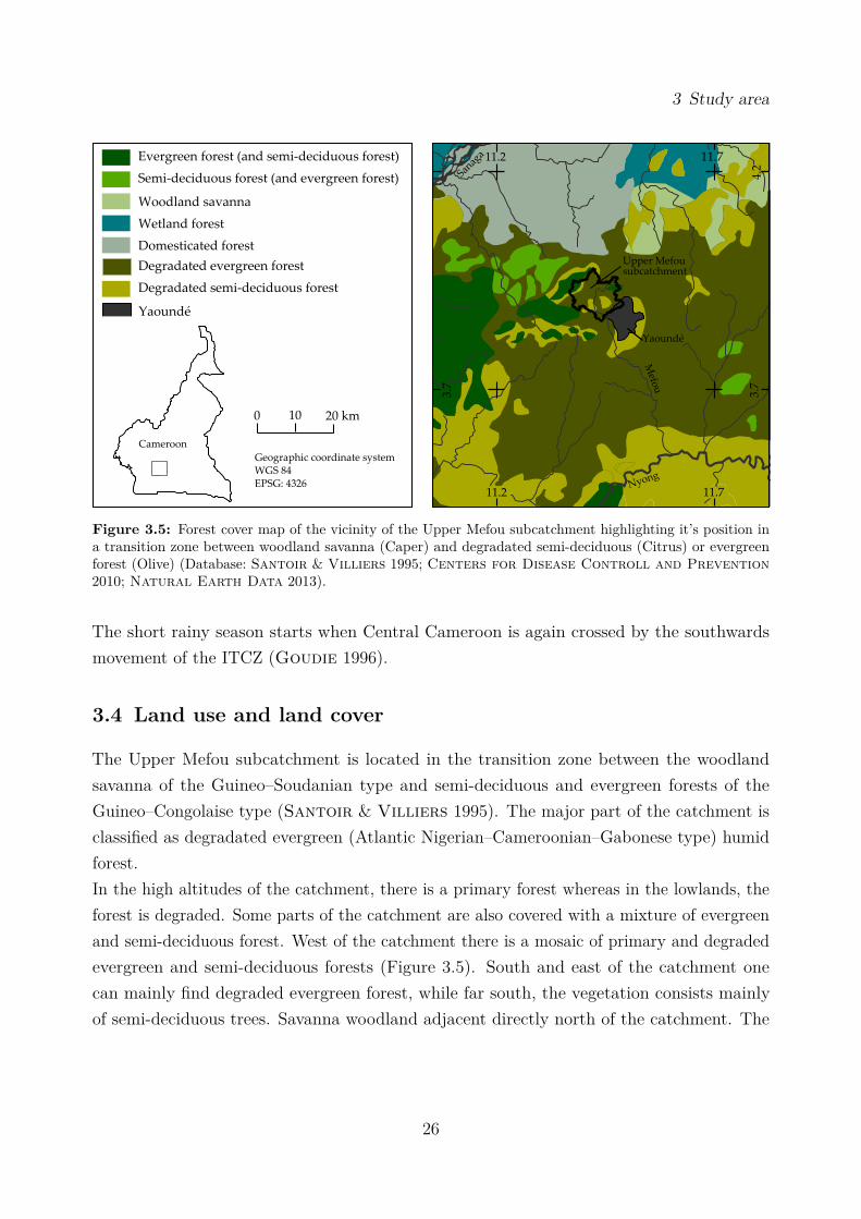
Figure 3.5: Forest cover map of the vicinity of the Upper Mefou subcatchment highlighting it’s position ina transition zone between woodland savanna (Caper) and degradated semi-deciduous (Citrus) or evergreenforest (Olive) (Database: Santoir & Villiers 1995; Centers for Disease Controll and Prevention2010; Natural Earth Data 2013).
The short rainy season starts when Central Cameroon is again crossed by the southwardsmovement of the ITCZ (Goudie 1996).
3.4 Land use and land cover
The Upper Mefou subcatchment is located in the transition zone between the woodlandsavanna of the Guineo–Soudanian type and semi-deciduous and evergreen forests of theGuineo–Congolaise type (Santoir & Villiers 1995). The major part of the catchment isclassified as degradated evergreen (Atlantic Nigerian–Cameroonian–Gabonese type) humidforest.In the high altitudes of the catchment, there is a primary forest whereas in the lowlands, theforest is degraded. Some parts of the catchment are also covered with a mixture of evergreenand semi-deciduous forest. West of the catchment there is a mosaic of primary and degradedevergreen and semi-deciduous forests (Figure 3.5). South and east of the catchment onecan mainly find degraded evergreen forest, while far south, the vegetation consists mainlyof semi-deciduous trees. Savanna woodland adjacent directly north of the catchment. The
26
3 Study area
lowlands around the Sanaga river are covered with floodplain forests or domesticated forests(Santoir & Villiers 1995).The forest in the study area is used for hunter and gatherers activities and for splash-and-burn agriculture. Food crops are produced on relatively small plots, which are typical foragriculture in southern and central Cameroon (Yemefack et al. 2006). Cultivated patchesare merged with primary and secondary forest as well as bush, fallows and plantations toa land cover mosaic. 13 to 15 patches per square kilometre are not seldom for the area(Yemefack et al. 2006). The most important crops are cassava (local name: mbon, binomialname: Manihot esculenta), maize (fon, Zea mays), groundnut (owondo, Arachis hypogea),sweet potato (mebouda, Ipomoea batatas) and tannia (mekaba, Xanthosoma sagittifiolium)(local names according to Mutsaers et al. 1981).Monocropping of maize or cassava are the most frequent forms of cropping, while variousforms of multiple mixed intercropping can be found (in order of abundance; own mapping,Nov/Dec 2012):
Taro (atu, Colocasia esculenta), okra (bitetam, Hibiscus esculentus), bitterleaf (ndoleh,Vernonia spp.), chili pepper (ondondo, Capsicum frutescens), tomato (ngoro, Lycopersiconesculentum) and fruit or oil trees like African oil palm (biton, Elaeis guineensis), papaya(fofo, Carica papaya), mango (Mangifera spp.) or plantain (ekon, Musa Plantain) are alsointercropped. The main-plants are mostly maize or cassava. Groundnut, cassava and maize
Table 3.1: Cropping calendar and rainfall during growing seasons. Timing and duration of work stepsaccording to farmer’s information, own observations and Nounamo & Yemafack (2000). An asterisk (∗)marks a month in which only cassava is planted. Mean rainfall of months in Nkolbisson (1956–1980; ComiteInterafricain D’Etudes Hydrauliques & Office de la Recherche Scientifique et TechniqueOutre-mer Service Hdrologique n. d., Comite Interafricain D’Etudes Hydrauliques et al. 1990).
Figure 3.6: Land cover in the rural (division Lekié) and periurban parts of the catchment (subdivisionsYaoundé II and VII). Note the low frequency of fallows and the higher extent of cropping areas in theperiurban part. Percentage of patches does not allow a statement about area proportions. Cropping areasin the periurban parts tend to be bigger than in the rural areas, where bush and forest patches are bigger(Source: own observations, Nov/Dec 2012).
are often grown on ridges, cassava also on small mounds. It is assumed that on mounds andridges, yields are higher (Howeler et al. 1993). Ridges are either contour parallel or not.Accordingly to the two distinct rainy seasons, there are also two growing seasons. Clearing forthe 1st growing seasons “essep” starts during the long dry period in December and January.Felling and burning begins in January and is normally finished until the end of February.Planting and seeding of the most crops takes place in March and April. In the Upper Mefousubcatchment, cassava is planted also in May, the month in the long wet season receiving mostrain (211mm). Also when the other crops are planted, rainfall is relatively high (Table 3.1).The crops of the first growing season are regularly harvested in July. The second growingseason “oyon” starts in June or July, felling and burning takes place during July and August,planting in August and September and harvesting in November or December. Again, cassavais planted somewhat later, in October.In the traditional shifting cultivation system, after one year of cultivation, fallowing starts.The typical plant succession of a fallow duration of 15–25 years (forest fallow) is crops andweets, grasses and herbs, woody herb, shrubs and trees (bush fallow) succeeded by forest(Nounamo & Yemafack 2000). Nevertheless, in the Upper Mefou subcatchment, the fallowperiod is often shorter. According to farmers, fallow duration is 1 to 15 years in the ruralparts of the catchments, while in the dense settled periurban parts and around the MefouReservoir, the fallow period is much shorter (1–6 yrs). Fields are often not cultivated for oneyear, but for up to 4 years. The rotation intensity (Ruthenberg & MacArthur 1980) is
28
3 Study area
therefore relatively high: In the rural parts, traditional shifting cultivation is still practiced;in the periurban parts, land use has often changed to semi-permanent cultivation (60% ofthe farmers) or even stationary cultivation with fallowing (20%). Only 20% of the farmerspractice shifting cultivation (personal communication with farmers in Nov/Dec 2012). Thisshift is not uncommon in central or southern Cameroon. Brown (2004) reports that in avillage in the vicinity of Yaoundé, two-thirds of the households do not practice forest fallow(>15 yrs), whereas it is practiced by three-quarters of the households in remote villages. Inanother study, which also covers the Mefou catchment, the shortening of fallowing (3–5 yrs) inthe more populated areas is observed for a long time (Mutsaers et al. 1981). A shorteningof the fallow period is explained by population pressure, a growing preference to fields closeto the villages and the expansion of cash crops (Nounamo & Yemafack 2000; Brown2004). As it is shown in Figure 3.6, fallowing is more common in the less populated ruralareas of the Mefou catchment than in the dense populated (periurban) areas . Also thecropping intensity is higher close to Yaoundé, whereas cash crop production (cacao, coffee) ismore common around the villages.
29
4 Methods and materialsThe study on hand focuses on three main objectives: The assessment of the actual andpotential soil erosion risk in the Upper Mefou catchment using the RULSE3D and anerosion/deposition index, the simulation of the impact of future land use scenarios on theerosion risk and the evaluation of the applied methods in a humid tropical catchment. Theevaluation includes a semi-quantitative validation of the erosion model results—a reservoirsediment survey—and a discussion of the values: comparison with values from literature anda sensitivity analysis. The main work flow is depicted in Figure 4.1.
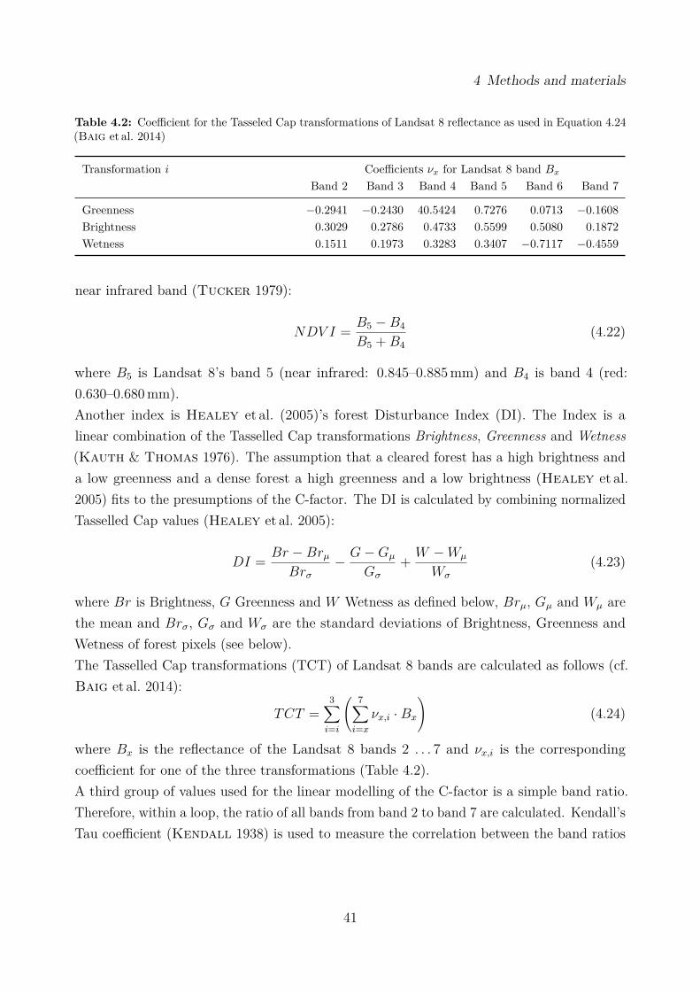
4.1 (Revisited) Universal Soil Loss Equation
The main focus of the study at hand is erosion modeling. During field work in November andDecember 2012, soil samples were collected, land use was taken down and sediments in theMefou Reservoir were observed. In addition, some non-structured interviews were conductedwith the help of a local interpreter.Erosion is modeled using the RUSLE3D, a three-dimensional enhancement of the RUSLE forthe catchment scale. The RULSE3D is principally based on the USLE, but the topographicfactor LS is replaced by a modified LS-factor, which can easily be computed in a GISenvironment and is suitable for a catchment-scale application of the USLE/RUSLE.In the original unit-plot-based USLE, soil loss (E0) is a function of rainfall erosivity and soilerodibility (Wischmeier & Smith 1978):
E0 = K ×R (4.1)
where K is a measure of soil erodibility in ton acre h 100−1 acre−1 ft−1 tonf−1 in−1 and Ris a measure of the rainfall erosivity in 100 ft ton-force in ac−1 h−1 yr−1. If the area underconsiderations deviates from the unit plot, Equation 4.1 has to be adjusted. Soil loss is thancalculated by multiplying E0 with ratios of the deviation of parameters different from theunit plot (Wischmeier & Smith 1978).
Assessment of the actual and potential soil erosion risk in the Upper Mefou subcatchment
O b j e c t i v e 2
Erosive impact of future land use
O b j e c t i v e 3Suitability of methods (for the humid tropics)
ValuesUofUKUTandURéUKéUCéULSRUformULiteature
Soil loss values (Acutal risk)
Figure 4.1: Flow chart of objectives, methods and materials. Parallelograms show input/output, rectanglesmeasurements (tiny contours) or main calculations (bold contours); ex expected main results are depictedwith filled parallelograms.
31
4 Methods and materials
where LS is a topographic factor, C a cover and crop management factor and P a soilconservation factor. The principles of determining K, R and the adjustment factors aredescribed in the following sections.
4.1.1 Rainfall erosivity factor (R)
As in the original version of the USLE, rainfall erosivity is expressed by the product of thetotal storm energy (E) times the maximum thirty minutes intensity (I30) in the RUSLE,where E is a function of the rainstorm intensity I. The calculation of I and therefore theR-factor requires the availability of high resolution pluviographic data. In the Upper Mefousubcatchment and it’s vicinity, such data is not available. The rain gauge data from thestation at Nkolbisson covers a period of 20 complete years of daily data (8458 days, Table 4.1).The station at Yaoundé covers a time series of 71 complete years of monthly data (1030 month,Table 4.1). Thus, the R-factor values of the Upper Mefou subcatchment have to be estimatedusing a validated regression.In the following, a set of approaches to approximate the R-factor is presented. These modelsare more or less specific for Cameroon, the humid tropics or at least West Africa. Anadditional overview of methods for R-estimations can be found in Borrelli (2011) and aspecific overview for Africa in Renard & Freimund (1994).Using the equation, special attention has to be paid to the units used. Some equationsare originally in US customary units (hundreds of foot tonforce inch acre-1 hour-1 year-1)and some in metric (SI) units (Megajoule millimetre hectar-1 hour-1 year-1). Also there aregood reasons to use the US system (Renard & Freimund 1994), in the thesis on handmetric units are used. To convert results of an equation in US-units, a conversion factor ofκR = 17.02 is used (Foster et al. 1981).
Roose’s rough approximation
One of the oldest and simplest approximation of the R-factor is the well established equationof Roose (1977):
R = Pa · (0.5± δ) · κR (4.3)
where Pa is the total annual precipitation, δ = 0.05 is a 5%-error and κR = 17.02 is theconversion factor.
32
4 Methods and materials
Table 4.1: Description of the rainfall stations and the data set used to calculate rainfall erosivity. Data fromYaoundé were download from the Koninkijk Nederlands Meterologisch Instituut (KNMI) Climate Explorer(climexp.knmi.nl).
01/1913–12/1926Data set Peterson & Vose (1997)∗ Comite Interafricain D’Etudes
Hydrauliques & Office de laRecherche Scientifique etTechnique Outre-mer ServiceHdrologique (n. d.)Comite Interafricain D’Etudes Hy-drauliques et al. (1990)
WMO station code 64950 –∗ Global Historical Climatology Network prcp from v2.prcp in v2.temperature.inv
The equation is based on a data set of 20 rainfall recording stations in West and CentralAfrica. It is not valid for coastal areas, mountainous regions and the transition zone betweenunimodal and bimodal rainfall distributions (Renard & Freimund 1994).
Modified Fournier Index
A second widespread erosivity index is Fournier’s index (Fournier 1960).
FI = Pmw2 · Pa−1 (4.4)
where FI is Fournier’s Index, Pmw is the amount of rainfall in the wettest month in a year inmillimetres and Pa is the total annual rainfall in millimetres.The index is often criticized due to it’s low reflection of erosivity (Morgan 2009). Thecontribution of other months than the wettest to erosion is underestimated by the index.Therefore, Arnoldus (1980) developed a new index, the Modified Fournier Index. Thisindex considers the rainfall of all months. Here, the increase of the rainfall in a month other
33
4 Methods and materials
than the wettest causes an increase of the erosivity value.
MFI =12∑i=1
(Pm2 · Pa−1) (4.5)
where MFI is the Modified Fournier Index, Pm is the amount of rainfall in a month m inmillimetre and Pa is the total annual rainfall in millimetre.To use the MFI in the RUSLE, the values have to be transformed into R-values. Onetransformation is modeled by Renard & Freimund (1994), which is based on the relationshipbetween MFI and measured R-values. Arnoldus (1980) used a similar relationship forAfrica. He found out that the correlation between FI and R at 14 not further describedstations in West Africa is relatively low (r = 0.36) . The regression between the MFI and Ris in contrast much better (r = 0.83) for the same stations.
R = 5.44 ·MFI − 416 (4.6)
A rainfall–R relationship for Cameroon
Bresch (1993) calculated a relationship between annual rainfall amounts and erosivity forCameroon. This regression is based on 18 stations in the semi-humid to humid parts of WestAfrica and Central Africa where rainfall totals 700–4000mma−1 (3–14 years; r2 = 0.91).
R = (11 + 0.012 · Pa)2 (4.7)
Salako’s model
A more spatially specific model to estimate the R-factor of the RUSLE was developedby Salako (2006). He uses long term pluviograph data from Ibadan and Onne (Port-Harcourt), both in Nigeria, to calculate the R-factor according to the procedures describedin Wischmeier & Smith (1978) or Brown & Foster (1987). These erosivitiy values areused to model the regression for daily and monthly data (Salako 2006):
R = a · P b (4.8)
where P is the rainfall amount in millimetre and a and b are site specific empirical modelparameters.
34
4 Methods and materials
For the humid forests in southern Nigeria a and b were calculated using the Port-Harcourtdatabase covering a period of 18 years or 2 106 days and a mean annual rainfall averaging2417mm (Salako 2008; Salako 2010) using Wischmeier’s storm erosivity index:
Ri = 0.130 · Pa1.070, Ri =365,366∑n=1
(0.113 · Pd1.205) (4.8a,b)
where Ri is the annual erosivity of a year i, Pa is the annual rainfall amount and Pd is thedaily rainfall amount.Values for a or b using the Brown–Foster Index are 0.223 or 2.057 for daily data an 0.302 or1.462 for annual rainfall data (Salako 2010). The coefficient of determination (r2) of allregressions is 0.97–0.98 (Salako 2008; Salako 2010).
African Rainfall Erosivity Subregional Empirical Downscaling (ARESED, Diodato et al.2013) is based on high resolution erosivity calculations over a long time span for severallocations in Africa. The information is interpolated and relationships between latitude,longitude and elevation are used to represent the spacial variability of rainfall over Africa.The horizontal spacial variability is a function of the seasonal migration of the InnertropicalConvergence Zone (latitude) and the higher energy load of heavy rainfall events in westernAfrica (Lal 1985). A weighted geographical scale factor (η) is developed by Diodato et al.(2013) to incorporate the variability in ARESED:
η = H · Z (4.9)
where H is a horizontal component and Z is a vertical component;
H = a · ϕ− b · λ3 + γ (4.10)
where ϕ is the latitude in decimal degree south, λ is the longitude of the study area in decimaldegree east, a = 0.01 and b = 0.00003 are scale parameters and γ = 10 is a shift parameter;
Z = 1−∆ · E (4.11)
where E is the elevation of the study area in metre above sea level and ∆ = 0.001 is anelevation scale parameter.
35
4 Methods and materials
The RUSLE’s rainfall erosivity factor (R) is (Diodato et al. 2013):
RARESED = η · φ · P85 · c (4.12)
where P85 is the 85%-percentile of the monthly precipitation data in millimetre, φ = 1 isa regional scaling operator and c = 1.271 is a shape parameter (Renard & Freimund1994).
4.1.2 Erodibility factor (K)
An erodibility nomograph (Wischmeier et al. 1971) is the most widely used tool to approxi-mate the erodibility factor K. In the USLE, erodibility is a function of grain size, organicmatter, soil structure and permeability. As presented in the RUSLE Handbook (Römkenset al. 1997), the nomograph can be replaced by an algebraic approximation of the K factor(Wischmeier & Smith 1978) if the silt fraction does not exceed 70%.
whereKalg is the approximated erodibility of the RUSLE K-factor nomograph in US customaryunits ( ton acre h 100−1 acre−1 ft−1 tonf−1 in−1 ), OM is the content of organic matter inpercent, mS is the fraction modified sand in percent (0.100–2.000mm, or very coarse sandto fine sand following the USDA size separates in percent; Soil Survey Division Staff1993), mU is the fraction modified silt in percent (0.002–0.100mm, or very fine sand and siltfollowing the USDA size separates; Soil Survey Division Staff 1993), s is the structureclass and p is the permeability class.The values can be converted to SI units using a conversion factor of κk = 7.59−1.As an application of the K-factor for relatively clay-rich, aggregated tropical soils is underdiscussion (El-Swaify et al. 1982; see Section 2.1) many approximations are used to betterrepresent the erodibility of these soils. In the study at hand, Nill (1993)’s approximationfor tropical soils is used, which has been tested in Cameroon for soils similar to the soil inthe Upper Mefou subcatchment.
Ktrop = a ·Kalg + b (4.14)
where Ktrop is an erodibility factor adapted to tropical conditions, Kalg is the K-factorapproximated as described in Equation 4.13 and a and b are soil specific parameters.
36
4 Methods and materials
Nill (1993) classified tropical soils from Cameroon and Nigeria into three groups with specificparameters. A soil is classified into one group where the following equations give the highestvalue:
where X1, X2 and X3 are the different groups, U is the fraction silt in percent, BD isthe bulk density in a depth of 5–10 cm in gramm per cubiccentimeter, OM is the contentorganic matter in percent and AGG is the content of dry-sieved 0.630–0.200mm aggregatesin percent.Bulk density was not measured for the soils in the Upper Mefou subcatchment during fieldwork. Therefore, mean empirical values from Nill’s study are used here (BD is 0.87 for X1
and X3 and 1.06 for X2). The same applies to pH (pH is 5.3 for X1, 5.1 for X2 and 5.0 forX3).The soil specific parameter a is 2.3 for group 1, 1.1 for group 2 and 0.03 for group 3; parameterb is 0.12 for group 1, 0 for group 2 and 0.006 for group 3 (Nill et al. 1996).
Grain size analysis
Modified silt and modified sand content are analysed by sieving and laser diffraction using aBeckman Coulter LS 13320 PIDS. The method is based on the assumption that the angleof laser diffraction of a particle decreases with increasing particle size. 117 detectors recordthe diffraction at a specific angle. Thus, the fraction of particle volume for each detectorand it’s mean grain size can be calculated based on the Frauenhofer theory and the Mietheory. The sample are sieved to the <1mm fraction and 2 g of each sample pretreatedseveral times with hydrogen peroxide (30% H2O2) to dissolve all organic material (Grayet al. 2010). As the samples have a relatively high content of organic material and fine grainfractions, dissolution is slow. To fasten up the process and to ensure that all organic materialis dissolved, the samples are put in a tempered shaking water bath. Water is separated fromthe samples by centrifugation to reinforce concentration levels of hydrogen peroxide. Whenno reaction is visible any more, the samples are divided and particle size is measured withthe Beckman Coulter. Two measurement runs are done per sample. The Beckman Coulteritself measures threefold; altogether a sixfold determination is done: mean values are used for
37
4 Methods and materials
further calculations. Additionally, three samples are also measured without pretreatment toverify the effect of non-removed organic material on grain size distributions.
Organic matter content
The organic matter content (OM) of 47 samples is analyzed by measuring total inorganiccarbon (TIC) and total carbon (TC):
OM = f · TOC = f · (TC − TIC) (4.16)
where TOC is the total organic carbon content in percent and f is a conversion factor.The “van Bemmelen factor” (f = 1.724) is often used for conversion, which traces back toSprengel 1826 (Pribyl 2010). A review of Pribyl (2010) shows that this factor is oftenmisused and lines of evidence in it’s calculation are not comprehensible. So in the study onhand, a more reliable factor f = 2 (Pribyl 2010) will be used, based on the assumption thatorganic material consists of 50% organic carbon.Total organic carbon is calculated as the difference between total carbon and inorganiccarbon. Total inorganic carbon is measured using a Carmhograph C-16 (co. H. WoesthoffMesstechnik). The fundamental operational principle is digestion in phosphoric acid (H3PO4)at a temperature being approximately 70 °C, the transfer of the released carbon dioxide indiluted sodium hydroxide and measurement of electrical conductivity differences of treatedand untreated sodium hydroxide. The conductivity difference of standards with a known TICcontent are used for a linear model of TIC values and conductivity differences (Appendix, p. iii).A LECO Truspec CHN–elemental analyzer is used to measure TC. The apparatus combuststhe sample in a stream of oxygen at 950 °C and uses an IR-detector to calculate the contentof TC from the CO2 concentration. Various standards are used for calibration.
Permeability
To calculate hydrological conductivity a Mini Disk infiltrometer (Decagon Devices, Inc.) wasused during field work. The volume of water infiltrating in the soil is measured at a specificinterval and a defined suction rate. As the suction rate is the a function of porosity, theselection of an adequate rate is texture-dependent. Because the soils in the study area havesandy texture, a suction rate of 2 is chosen (Decagon Devices 2012). The time intervalis adapted to the total duration of measurement. Up to 5 minutes, the level of the watercolumn is taken down every 0.5 minutes. In slow infiltrating soils, the level is taken downevery 2.5 minutes or every 5 minutes after 5 minutes.
38
4 Methods and materials
Hydraulic conductivity (k) is determined following the method of Zhang (1997):
k = CtAk
(4.17)
where Ct is the slope of the graph of cumulative infiltration at the time t against the squareroot of time (
where α and nk are the van-Genuchten parameters (Van Genuchten 1980), h0 is thesuction rate and r0 = 2.25 cm the radius of the mini disk; z is 2.92 for n ≥ 1.9 and 7.5 fornG < 1.9.The van-Genuchten parameters are taken from Carsel & Parrish (1988: p. 759). Ct isdetermined by a quadratic regression (2nd degree polynomial regression; Decagon Devices2012).
It = Ct ·√t2 + b ·
√t (4.19)
where b is a model parameter and It is the cumulative infiltration at time t.The quadratic regression is solved with the function nls of the stats-package in R (R CoreTeam 2013).
4.1.3 Land cover and management factor (C)
A Landsat 8 image is used to calculate the land cover and management factor (C). The imageis preprocessed and spectral information of pixels with well known C-factor information fromground-truthing is used to calculate a linear model of spectral information and the C-factor.The relationship calculated from the sampled point is than used to predict C-factor valuesfor the entire image; the predicted values are validated with a second set of ground-truthinformation.
Landsat 8 image
Landsat 8 is a medium-resolution satellite system and part of the Landsat continuity mission(30m resolution). Observations of the sensor Operational Land Imager (OLI) are similarto those of the previous sensor (EMT+). The bands of Landsat 8 are somewhat morenarrow than the bands of ETM+; two additional are added: a shorter blue wavelength bandand a second short infrared band for cirrus detection. Landsat 8 has 11 bands including
39
4 Methods and materials
two thermal bands and a panchromatic band (15m resolution). Wavelength informationis given below if necessary; descriptions of the system can be found in Irons et al. (2012)for the announcement of Landsat 8 and Roy et al. (2014) for details. The Landsat 8 sceneLC81850572014137LGN00 (WRS-path 185, WRS-row 57) used here was acquired on May5th 2014 and is clipped to the extent of the study area.
Landsat 8 preprocessing
Radiometric calibration of the Landsat 8 scene is done separately for each band. Due tothe fact that the raw scenes as provided by the USGS and available via the Earth Explorerconsist of quantized and calibrated scaled digital numbers (DN), the values at first have tobe converted to top-of-the-atmosphere reflectance (US Geological Survey 2013):
ρλ = Mρ ·DN + Sρsin θSE
(4.20)
where ρλ is the top-of-the-atmosphere planetary reflectance, Mρ is a band-specific multiplica-tive rescaling factor, Sρ is a band-specific additive rescaling factor, DN is the digital numberand θSE is the local sun elevation angle in degree.The rescaling factors and the sun elevation angle for the specific Landsat scene are givenin the meta data of the scene. All bands instead of temperature bands and the QualityAssessment (QA) band are calibrated.The 16-bit information of the QA band is used to detect clouds in the image; Bits 14 and 15can be translated to a confidence that the condition “cloudy” is fulfilled (00 is no cloud, 01 isa low confidence of clouds, 10 is a medium confidence of clouds and 11 is a high confidence ofclouds). In the study on hand, only high confidence of clouds are used to mask the clouds.Cloud shadows are masked using the normalized ratio of the short wavelength Coastal/AerosolBand 1 (B1) to Band 2 (B2) (Yale Center for Earth Observation 2013):
ACI = B1 −B2
B1 +B2(4.21)
Shadows have relatively high values. A non-shadow–shadow threshold is defined by a visualinterpretation of a true colour displayed Landsat scene.
Transformations, ratios and indices
Normalized Difference Vegetation Index (NDVI) values are often used to model C-factorvalues (De Jong 1994; Erencin 2000). The NDVI is the normalized ratio of the red to the
40
4 Methods and materials
Table 4.2: Coefficient for the Tasseled Cap transformations of Landsat 8 reflectance as used in Equation 4.24(Baig et al. 2014)
Transformation i Coefficients νx for Landsat 8 band Bx
where B5 is Landsat 8’s band 5 (near infrared: 0.845–0.885mm) and B4 is band 4 (red:0.630–0.680mm).Another index is Healey et al. (2005)’s forest Disturbance Index (DI). The Index is alinear combination of the Tasselled Cap transformations Brightness, Greenness and Wetness(Kauth & Thomas 1976). The assumption that a cleared forest has a high brightness anda low greenness and a dense forest a high greenness and a low brightness (Healey et al.2005) fits to the presumptions of the C-factor. The DI is calculated by combining normalizedTasselled Cap values (Healey et al. 2005):
DI = Br −BrµBrσ
− G−Gµ
Gσ
+ W −Wµ
Wσ
(4.23)
where Br is Brightness, G Greenness and W Wetness as defined below, Brµ, Gµ and Wµ arethe mean and Brσ, Gσ and Wσ are the standard deviations of Brightness, Greenness andWetness of forest pixels (see below).The Tasselled Cap transformations (TCT) of Landsat 8 bands are calculated as follows (cf.Baig et al. 2014):
TCT =3∑i=i
( 7∑i=x
νx,i ·Bx
)(4.24)
where Bx is the reflectance of the Landsat 8 bands 2 . . . 7 and νx,i is the correspondingcoefficient for one of the three transformations (Table 4.2).A third group of values used for the linear modelling of the C-factor is a simple band ratio.Therefore, within a loop, the ratio of all bands from band 2 to band 7 are calculated. Kendall’sTau coefficient (Kendall 1938) is used to measure the correlation between the band ratios
41
4 Methods and materials
and the C-factor values of the training data set (see below). The ratio with the highestcorrelation coefficient will be chosen for further analysis.
Linear models
General linear models are calculated to test the relationship between the C-factor from atraining data set with well known C-values and the indices and ratios.The training dataset contains a total number of 69 ground-truth point samples, of which 37are classified as dense forest and 32 as bare ground (C-factors 0.002 and 1.000; cf. El-Swaifyet al. 1982). These samples are visually interpreted Google Earth views, which are drawnusing the OpenLayers Plugin (Kalberer & Walker 2014) in QGIS 2.0.1 Dufour (QGISDevelopment Team 2013). A validation data set is generated the same way; the samplepoints of both are shown in the Appendix (p. v). The validation data set consists of 28 pointsclassified as dense forest and 25 as bare ground.Linear models are calculated using the Fitting Linear Model function in R (R Core Team2012). A visual interpretation of residual vs fitted values, a Scale–Location plot, a NormalQ–Q plot, a plot of the square root of the model residuals against the fitted values and aplot of Cook’s distance against leverage are used to test the model assumptions. In thecase the models do not meet the assumptions of normal distribution of the residuals andhomoscedasticity, the response variable C-factor is Box–Cox transformed (Box & Cox1964). For predicting the C-factors of the entire grid, the values will be transformed againif −1 ≥ lambda < 0.5. Otherwise, no re-transformation is necessary (Thome 2005). Theprediction of C is based on the regression equation given by the linear model.The estimated C-factor grid is reclassified in a last step. C-factor values below 0 and above 1are not possible by definition, so all values less than 0.002 are set to 0.002 (dense forest) andall values above 1 to 1.000 (bare ground).
4.1.4 Topographic factor (LS)
The dimentionless topographic factor (LS) of the RUSLE3D is calculated using the approachof Mitasova et al. (1996). In contradiction to the original version of the USLE (Wischmeier& Smith 1978), this approach is based on upslope contributing area instead of slope length.Upslope contributing area is defined as flow accumulation per unit contour width (Mitasovaet al. 1996)—i. e., the length of the uphill pathes of converging flow (Desmet & Govers1997). In a grid-based algorithm, a unit contour width equals the resolution of the DEM.The original USLE’s LS-factor is the ratio of soil loss from the area under investigation tothe standard plot from a length of 22.13m and a slope of 9% (Wischmeier & Smith 1978).
42
4 Methods and materials
LS is here a function of slope length and slope angle:
LS =(λ
λ0
)m (65.41 sin2 β + 4.56 sin β + 0.065
)(4.25)
where β is the slope angle in percent rise over run, λ is the slope length in feet, λ0 = 72.6 ft =22.1m is the length of the standard plot and m is a dimensionless parameter, which in itselfdepends on the slope angle and is 0.5 for a slope angle of 5.0% or more, 0.4 for slopes of 3.5%to 4.5%, 0.3 for slopes of 1.0% to 3.0% and 0.2 for slopes of less than 1.0%.Mitasova et al. (1996) modified the equation based on the unit stream power theory (Moore& Burch 1986a) to incorporate flow convergence and replaced λ by Acont to calculate themodified LS-factor of a grid cell r:
LSr = (m+ 1)(Acontλ0
)m (sin ββ0
)n(4.26)
where β0 = 9% = 5.14 ° is the slope of the standard plot, λ0 = 22.13 m is the slope length ofthe standard plot, Acont is the upslope contributing area in metre and m = 0.1 and n = 1.3are dimensionless parameters, adapted to a high vegetation cover and the absence of a rillnetwork during field work (cf. Mitasova et al. 1996; Hoffmann et al. 2013).An ASTER Global Digital Elevation Model V002 (30m resolution; NASA and JapanASTER Program 2011) and a SRTM DEM (90m resolution; United States GeologicalSurvey (USGS) 2012) are used to calculate upslope contributing area and slope in RSAGA(Brenning 2008) an interface between the statistic software R (R Core Team 2013) andSAGA GIS (System for Automated Geoscientific Analyses; Böhner et al. 2006; Conrad2006).
DEM preprocessing
A Multi Direction Lee Filter, an enhanced version of Lee’s Sigma Filter (Lee 1983), is appliedin a first step to reduce speckled noise and outliers of the DEMs. The advantage of thisalgorithm is that noise is detected and reduced without reducing the terrain information;narrow valleys, linear information and slopes will be preserved (Lee 1983). The original SigmaFilter is based on the assumptions that noise of an image follows a Gaussian distributionand is not correlated to the neighbouring pixel values. The filter algorithm relies on localstatistics; values exceeding the prior local variances are not included in the posterior meansof the filtered image (Lee 1983). In SAGA GIS, a Multi Direction Lee Filter is implementedwhich applies a Sigma Filter on the directional neighbourhood with minimum variance (Lee
43
4 Methods and materials
et al. 1998). The 16 possible neighbourhoods are shown in Selige et al. (2006). For estimatedrelative and absolute noise as well as for weighting, RSAGA defaults are used.In a second step, sinks are filled in the filtered DEM to avoid flow to artificial depressions inthe DEM. For a better representation of the stream network in the Mefou subcatchment,a stream grid, which is based on rasterized stream lines from a topographic map (1:50 000;Institue Géographique National 1956), is burned into the DEM (ε = 1.5 m).The fill algorithm used here is the technique developed by Wang & Liu (2006), which usesspill elevation and low-cost paths to fill depressions. Spill elevation is defined as the minimumelevation which is necessary to compute a depressionless grid. The technique starts at a bordercell of a grid and progressively tests if the flow of each grid cell is connected to the border. Ifnot, the value of the cell will be raised to spill elevation. A least-cost search is applied tofind the flow direction of each grid cell (Wang & Liu 2006). The Wang-and-Liu–algorithmimplemented in RSAGA slightly modifies the spill elevation using a minimum slope of eachgrid cell (0.01 °) to avoid areas without flow.
Computation of LS
The preprocessed DEMs are used to calculate the two input variables of Mitasova et al.’sLS-factor.A slope grid is calculated according to the method of Zevenbergen & Thorne (1987),which is based on the 2nd degree polynomial adjustment. This method is recommended byGarcia Rodriguez & Gimenez Suarez (2012) among others to be used in USLE-familiyerosion models.Flow accumulation (or: catchment area, upslope area) is calculated using both MultipleFlow Direction (MFD; Freeman 1991; Quinn et al. 1991 and Deterministic infinity (D∞;Tarboton 1997). The results are used to evaluate the influence of algorithm selection onthe LS-factor. Algorithms based on single flow, e. g. Deterministic 8 (D8) (O’Callaghan& Mark 1984) or Rho8 (Fairfield & Leymarie 1991), are not used due to their limitedrepresentation of real flow patterns and the overrating of grid cells with slightly higherelevation (Seibert & McGlynn 2007). This is especially important when working withfilled DEM, where the spill elevations of neighboring grid cells have low differences.As D8 and Rho8, D∞ is principally based on a single flow direction. But in contrast to thefirst mentioned algorithms, flow direction is not considered to be from one center of a grid cellto another center, but defined as the “steepest downward slope on planar triangular facetson a block-centered grid” (Tarboton 1997). The flow direction can be everything between
44
4 Methods and materials
0 and 2π, considering that 0, π/2, π and 3π/2 are the cardinals and π/4, 3π/4, 5π/4 or 7π/4are the diagonals of a rectangle drawn between the centers of the eight neighboring cells.The flow accumulation to the ith downhill grid cell is calculated as a proportion of flowbetween two downslope pixels. The proportion is the proximity of the flow direction angle tothe direction angle of the grid cell center (Tarboton 1997):
Ai = α2
(α2 + α1) · Ai−1 (4.27)
where Ai is flow accumulation of the ith downhill grid cell, A is the flow accumulation of theupslope grid cell, α1 and α2 are the angle between the flow direction and the verticals of thetriangular facets in flow direction.Thus, flow dispersion to two of eight neighboring pixels is possible (for a detailed descriptionof the procedure see Tarboton 1997).The MFD-algorithm is based on the principal that the outflow of an uphill cell is distributedto all of the eight neighboring downhill cells with lower elevation (Freeman 1991). Theproportion distributed to each cell is a function of the slope angle between an uphill and adownhill cell (tan β) and the effective contour length of the flow direction (Li), which dependson whether the flow direction is cardinal or diagonal. The amount of flow accumulation inthe ith downhill cell (Ai) is (Quinn et al. 1991):
Ai = (tan βi · Li)8∑
k=1(tan βk · Li)
· Ai−1 (4.28)
Computation in SAGA GIS starts at the grid cell with the highest value and is done parallellydownwards (SAGA module: Catchment Area [Parallel]).Using the output grid of both algorithms, upslope contributing area (Acont) is calculatedby dividing the grid values with the grid cell size. LS is than computed as described inEquation 4.26.
4.2 Net deposition areas
Both USLE, and RUSLE/RUSLE3D calculate only net erosion—also on areas experiencingnet deposition. To avoid the problem of an overestimation of total soil loss, deposition areasare identified using a topographic erosion/deposition index, which is based on the transportcapacity limited Unit Stream Power Erosion Deposition (USPED) model (Mitasova et al.
45
4 Methods and materials
1996; Mitas & Mitasova 1998):
ED = d (T · cosψ)/ dx + d (T · sinψ)/ dy (4.29)
where ED is erosion or deposition, T = A is the soil loss modeled with the RUSLE3D and ψis the terrain aspect.The derivatives are calculated with a slope algorithm in a GIS (Mitasova & Mitas 1999;Hofierka et al. 2009). Rainfall erosivity, soil erodibility and cover/crop managment, T canbe replaced by the topographic factor of the RUSLE3D to consider only the topographicpotential (Hofierka et al. 2009):
EDLS = d (1.4 · L× S · cosψ)/ dx + d (1.4 · L× S · sinψ)/ dy (4.30)
Here, L× S is calculated with the parameters used in Mitasova et al. (1996):
L× S =(Acont
22.13 m
)0.4×(
sin β5.16°
)1.3
(4.31)
4.3 Simulations
For managing purposes in the context of IWM—or more specific water management—thesimulation of the effect of future land use and land cover changes (LULCC) on the environmentis a well known tool (Dekkers & Koomen 2007; Heathcote 2009). Based on modeledsoil loss and the NDVI-approximated C-factor, the effect of five LULCC-scenarios on soillosses is simulated in the thesis on hand. Maps will be drawn which highlight areas of highexpected impact. A change of the C-factor corresponding to the LULCC is used as simulationinput. All other values and factors (R, K, LS, P) are kept constant (cf. Nearing et al. 2005;Terranova et al. 2009); possible changes of soil erodibility as a result of a changed cover orsoil conservation strategies are not taken into consideration.
Scenario 1: Mixed-cropping extensification In Scenario 1, it is assumed that—possiblydriven by a higher demand for food for a growing population in rural or periurban areas—food production in the area is expected to increase by forest clearance or a cultivation ofbush or fallows. The expansion of mixed-forest systems and the associated deforestationis described—at least as an ongoing process—by Imbernon & Branthomme (2001) andLambin et al. (2003) for tropical rainforests in central Cameroon. In addition, Sunderlinet al. (2000) (cf. Sayer et al. 2012) note that the intensification of food crops is a strategy to
46
4 Methods and materials
cope with an economic crisis. As it is described in Section 3.4, field covers a higher proportionof the land around dense settled areas. The scenario is implemented in a soil erosion modelby a change of the C-factor from 0.001–0.01 to 0.23 (Scenario 1a) and from 0.01–0.10 to0.23 (Scenario 1b). C-factors 0.001–0.01 are typical for dense forest, well established densebush and natural savanna-like vegetation. Values from 0.001 to 0.01 are typcial values forforests in the area (Roose 1977; El-Swaify et al. 1982; Nill et al. 1996); a C-value of 0.23is typical for mixed cropping systems in the area of Yaoundé (Nill et al. 1996). The rangefrom 0.01 to 0.10 covers spares bush and short time fallows (Nill et al. 1996).
Scenario 2: Mono-cropping intensification The second scenario takes account of theintensification of cropping, i. e. mixed-cropping systems will change to cassava or maizemono-cropping. Thus, C-factor inputs for erosion modelling are changed from 0.18–0.28 to0.36 (El-Swaify et al. 1982; Nill et al. 1996). As in Scenario 2, the intensification might becaused by economical problems (Sunderlin et al. 2000; Sayer et al. 2012) and the generaltrend to more intensive crop production for the food supply of Yaoundé (cf. Kotto-Sameet al. 1997).
Scenario 3: More cash crops In addition to an intensification of food production, alsothe production of cash crops might increase. In Scenario 3 it is therefore assumed that forestor dense shrub is converted to plantations—either to coffee, cacao or palm oil plantationsfor cash food production or to plantains for food production. C-factors are accordinglychanged from 0.001–0.01 to 0.06 (El-Swaify et al. 1982; Nill et al. 1996) to simulate theextensification of cash crop production.
Scenario 4: Forest regrowth The last scenario simulates the erosional impact of refor-estation measures; C-factors from 0.18 to 0.41 (mixed-cropping systems or monocropping)are converted to 0.01 (forest/bush).
4.4 Semi-quantitative validation
Validation approaches of soil erosion models include field mapping of erosion features, remotesensing, erosion plots, radioactive isotopes such as Cs-137, measurement of river sedimentload and reservoir siltation measurements (cf. Borrelli 2011). Due to the fact that mostof the methods are too time consuming and/or too expensive for the scale of the study athand, a reservoir sedimentation study is applied to validate the erosion model, which wasencouraged by the release of the Mefou Reservoir during field work in 2012.
47
4 Methods and materials
The reservoir sedimentation study is based on two main input variables namely sedimentvolume and trap efficiency (Verstraeten & Poesen 2002). The sediment volume isestimated by the following equation:
sediment volume = reservoir surface area× thickness× bulk density (4.32)
Reservoir surface area is calculated with a Geographical Information System, sedimentthickness was measured during field work and is averaged for calculation and typical valuesof sediment bulk density are taken from the literature.Sediment mass has to be set in relation to the operation time of the reservoir, the catchmentarea and the trap efficiency of the reservoir (cf. Verstraeten & Poesen 2002):
where SSYr is the area specific sediment yield in the reservoir.Trap effieciency is approximated using the Brown curve (Brown 1943) as used in Morris(1998) and Verstraeten & Poesen (2000), which is more easy to apply for metric unitswithout conversion. In the Brown curve, trap efficiency is a function of the catchment–capacityratio.To validate the model, SSYr is compared with the area specific sediment yield of thecatchment (SSYc), which is calculated as a function of the proportion of erosion from slopesand settlements/roads (empirical values from literature), the modelled gross erosion (E) andthe sediment delivery ratio (SDR), also taken from literature.SDR expresses the percentage of erosion which is not stored in the catchment in wetlands,floodplains, on fields, in bufferstripes, in topographical depression or on foodslopes.
SSYc = SDR× A× proportion of field erosion (4.34)
Due to the fact that values from literature are not site specific, a set of normal distributedvalues is used for sediment bulk density, SDR and the proportion of erosion from fields (meansand standard deviation are the means and standard deviation of all literature values used).
4.5 Statistics and reporting of figures
Mean, standard deviation, range, quartiles, maximum, minimum and ranges are reportedas described in statistics textbooks (Bahrenberg et al. 2010). Means are always reportedplus/minus their standard deviation (x̄ ± s). The standard error of the mean (SEM) is
48
4 Methods and materials
calculated by dividing the standard deviation of a sample by the square root of the samplesize. Outliers are eliminated applying the procedure descriptive in Bahrenberg et al. (2010):A value i is not used for further calculation or descriptive statistics if the value does not fitin the range of the mean of the sample without the proposed outlier plus/minus the fourfoldstandard deviation of the sample’s mean. Due to the fact that there is no standard procedureto describe significant figures, an approach based on the SEM is used here: A figure of amean is considered to be significant if the same figure of the mean’s SEM is non-zero. Forsome indices or values, is common to report two digits (e. g. NDVI). In this case—althoughthe first/second digit is not significant—two digits are reported, but the last significantfigure is emphasized with an underscore (e. g. a mean NDVI-value 0.52 is reported as 0.52 ifSEM=0.11). A figure of measured values is only significant if the correction of a value by it’serror obtained from the measurement of a standard sample would not completely change theinformation of that figure.Test statistics are used to test for difference of sample means. A t-test is used if the twosamples are normally distributed and the variances are homogeneous; a Wilcoxon-rank-sum-test (Wilcoxon 1945; Mann & Whitney 1947) is used if the two samples are notnormally distributed, but variances are homogeneous. (Other cases didn’t appear.) To testfor normal distribution, a Shapiro–Wilk test (Shapiro & Wilk 1965) is used; homegenity ofvariances is tested using a Levene Test (Levene 1960) for non-normal distributed valuesand a F-test of Equality of Variances for normal distributed values (Cornillon et al. 2012).The computation of the RUSLE3D is completely done in R; for the scripts of the model seethe DVD-appendix.
4.6 Computation
All statistics are computed using R (R Core Team 2013). Except of the Levene test(levene.test), all statistics and tests are part of the base version of R. Default settingas proposed in R are kept. Image processing, handling and analysis is done in R. A listof packages is given in Table 4.3. Maps are prepared with QGIS 2.0.1 Dafur (QGISDevelopment Team 2013). Plots are drawn in R (Table 4.3). Other Figures as well asmaps are finally drawn in Inkscape 0.48.4 (Albert et al. 2013).
49
4 Methods and materials
Table 4.3: Packages used in R (R Core Team 2013) for data processing and graphical or tabular output.
Package Description Reference
landsat preprocessing of landsat imagery (image-based radiometriccorrection)
Goslee 2011
raster reading, writing, manipulation and analysis of grid baseddata
Hijmans 2013
rgeos vector geometry (shapefiles) Bivand & Rundel 2013shapefiles handling of shapefiles Stabler 2013sp handling geospacial data in R Pebesma & Bivand 2005;
Bivand et al. 2013brgdal handling of geospacial data Bivand et al. 2013astringr handling of strings (manipulation of Beckman Coulter data) Wickham 2012RSAGA SAGA GIS interface for R Brenning 2008car Levene testplotrix making nice plots using R Lemon 2006xtable export of data frames from R to LaTeX Dahl 2014
50
5 Results
5.1 Rainfall erosivity
Rainfall erosivity in the Upper Mefou subcatchment is estimated using different approaches anddata sets. In Table 5.1 the mean annual R-values of Nkolbisson and Yaoundé are shown. The R-values differ clearly. For Nkolbisson, the highest R-value (15 658MJmmha−1 h−1 yr−1) is calcu-lated using the approximation of Bresch (1993); the lowest value (10 015 haMJmmha−1 h−1 yr−1)is calculated using the daily regression for Nigeria (Salako 2008). The value range of Roose(1977) is 12 259–14 983. The data of the climate station in Yaoundé are quite similar tothose of the station in Nkolbisson, with one exception: While the mean annual R-value usingthe approach of Diodato et al. (2013) is 10 033 for Nkolbisson, the R-value for Yaoundé is13 766.The standard error of the mean (SEM) of the Yaoundé-values is much smaller, due to thefact that a large data set is used for the calculation. Also the SEMs of the models differ. Forthe approach based on the Modified Fournier Index and Bresch’s regression, the error isrelatively high, while the error is clearly smaller when applying the approaches of Roose(1977) or Salako (2008). Due to a higher variability in the daily data set, the error usingthe Salako (2006)-approach is higher than the regression based on annual data.For further calculations—either the seasonal fluctuation of rainfall erosivity or soil loss—theFoster–Brown-based daily erosivity model of Salako (2008) will be used for two reasons:Firstly, models based on daily data sets are more reliable (see Section 6.3.3; Angulo-
Table 5.1: R-factor values calculated on the basis of different algorithms (∗ rainfall kinetic energy EL30 acc.to Wischmeier & Smith 1978, † EL30 acc. to Brown & Foster 1987)
all days (boxes and astersiks)rainy days (bars and line)'erosive' days (bars)
long dry long wet short dry short wet long drySEASONS
Figure 5.1: Annual cycle of rainfall erosivity calculated using the approach of Salako 2010 on the basisof daily values from Nkolbisson. The upper plot shows the percentage of rainy days and days with rainfalltotals >12.7mm (Wischmeier & Smith 1978), the lower plot shows daily rainfall erosivity of each month inthe years 1952–1980; boxes include dry days, while lines (mean) and shades (standard error of the mean)include only rainy days.
Martínez & Beguería 2009) and allow the calculation of seasonal erosivity; secondly, theseR-values fit very well to the wide range of the Roose–approach, what is not true for allapproaches.The seasonal variation of the R-values is shown in Figure 5.1. The barplot shows the frequencyof rainy days (Pd > 0.1mm) and erosive days (Pd > 12.7mm; cf. Angulo-Martínez &Beguería 2009); the boxplots show the mean daily R-values in each month. The lineindicates the seasonal variability of the R-factor of rainy days. December, January andFebruary in the long dry season and July and August in the short dry season are the monthswith the lowest mean daily R-values.In March to June and September and October mean daily R-values are much higher. Thedispersion of mean daily R-values varies with the month. There are some years with highmean daily R-values in the wet seasons, but also months with low values. Variability ismuch smaller in the dry seasons, especially in January. The highest mean daily R-valueis calculated for October. In the short wet season, the proportion of rainy days is around
52
5 Results
Table 5.2: Monthly mean of daily rainfall erosivitiy [MJmmha−1 h−1 yr−1]
Jan Feb Mar Apr May Jun Jul Aug Sep Oct Nov Dec Mean
three third (September: 61%, October: 67%); in January, only 7% of the days are rainy, inDecember only 10% are rainy. R-values of rainy days are higher in the short than in thelong rainy season, as it is the case for mean daily R-values of all days. Erosive days arethe most frequent in Mai (19%) September (22%) and October (29%), whereas they areseldom in January (2%), December (2%) and July (4%). In the long rainy season—except ofJune—and the short rainy season, more than one third of the rainy days are erosive days.In October, 44% of the rainy days are erosive days. Although January is the month withsmallest proportion of rainy days and low mean daily R-values, the R-values on rainy daysare relatively high (Table 5.2). Months with a high mean erosivity and a high proportion ofrainy or erosive days have also a higher erosivity of the rainy days. Erosive days of thesemonth are considerably less pronounced more erosive. Erosivity of erosive days in the longdry season is not clearly less than in some months of the long wet season (Table 5.2).
5.2 Soil erodibility
Organic matter
The measured organic matter content of 46 samples ranges from 1.6% to 9.4% with a mean of5.2± 1.8 pp. The highest OM values are measured on a fallow, a forest with intergrowing oilpalms, on a cacao plantation and on a mixed plantain–palm plantation (samples Nk13, NK26,Nk22 and Nk7). In contrast, samples with low OM values (<3%) are from maize–groundnutfields (Nk35), from mix-cropping fields with cassava as main plant and sweet potato orMacabo as second plants (Nk11 and Nk36) or from a recent cassava fallow (Nk28). A t-test1
of equal means shows that plantations and forest/bush have a significantly higher meanorganic matter content than fields; mean %OM of fields is 4.2, while the mean of plantationsis 6.5 and the mean of forests is 6.6. The means of other combinations of land use types(fallow, field, forest and plantation) are not significantly different; the mean %OM of fallowsis 5.4. The samples with a low OM content were collected around the Mefou Reservoir or inthe urban parts of the Upper Mefou subcatchment.
1deviance of %OM from normal distribution is rejected using a Shapiro–Wilk test (W=0.98, p>0.1);homogeneity of variances is confirmed with a F-test (F3−14,4−5=0.3889–1.7446, p>0.38)
53
5 Results
Permeability
Range and dispersion of permeability is very wide. The minimum value is ca. 0.016·10−3 cm s−1,measured in a forest with palms on a sandy loam. The maximum value of 3.290 · 10−3 cm s−1
is measured on a tomato field (Nk3: sandy loam). The mean permeability value is 0.5 ±0.6 10−3 cm s−1. For the use in the RUSLE, the values are classified in six permeability classesaccording to the National Soil Survey Handbook (NSSH) No. 430 (USDA 1983; Römkenset al. 1997). The majority of soils under investigation are classified as moderate, moderate torapid or slow to moderate infiltrating. Two soils are classified as rapidly infiltrating, whilefive soils, mainly covered with semi-natural vegetation or plantations, are classified as veryslow infiltrating. As it is shown in Figure 5.2, conductivity of a soil is a function of land useand land cover.Forest and bush soils have the lowest conductivity, while conductivity is higher on plantationsand fallows. The highest values are measured at fields, where the dispersion of the values isvery high; both relatively low values and high values are measured. The mean permeabilityof fields and forests or of fields and plantations differ significantly (Wilcoxon rank-sumtest, W=70 or W=95, p<0.05)2. The means of fields and fallows and fields, forests andplantations and forests and plantations do not significantly differ (W=12–19, p>0.05). Onfive fields with ridge tillage, infiltration was tested on the ridges and on the pathes betweenthe ridge. Conductivity values are up to ten times higher on ridges at three sides. Incontrast, on two ridges conductivity is up to twice lower in comparison with the intermediatepath. The mean conductivity on ridges is 0.66 · 10−3 cm s−1 , whereas the mean conductivityon the intermediate paths is 0.32 · 10−3 cm s−1. In relation to the high dispersion of theconductivity values (x̄ = 0.5±0.6 ·10−3 cm s−1) and the range of values as shown in Figure 5.2,neither values on ridges (0.3–1.27± 0.6 · 10−3 cm s−1) nor values on intermedia pathes (0.03–0.66 ± 0.6 · 10−3 cm s−1) are—except of one value—extraordinary high or extraordinarylow.
Grain size
The grain size of 38 samples is measured using laser diffraction. Expect of a few samples, allgrain size distributions have a similar shape. Sample Nk26 shows differences between thefirst and the second run, but mean values seem to be similar to the other results. Three
2Conductivity values differ significantly from normal distribution (Shapiro–Wilk test, W=0.643, p<0.05);the permeability- variances of the land use and land cover types are homogeneous (Levene’s Test forHomogeneity of Variance, F3,29=1.07, p>0.05). Thus, the Wilcoxon test is applied here
54
5 Results
●
●
Hyd
raul
ic c
ond
ucti
vity
[10
−3 c
m s
−1 ]
00.
10.
40.
91.
62.
53.
6
Fallow Field Forest/bush Plantation
Figure 5.2: Infiltration rates on different land use types. Note the non-linear scaling of the y-axis.
samples (Nk8, Nk18, Nk10F) have an extraordinary high content of fine silt (2–20 µm). Themean grain size distribution and the dispersion of sizes are shown in Figure 5.3.An average sample contains 11% clay, 22% silt and 67% sand, whereas the most frequentgrain size separate is medium sand (21%), followed by fine sand (19%) and coarse sand(18%).The variability between the samples is relatively low in the clay fraction and the coarsesilt to fine sand fractions, while in the fine silt fraction and especially in the medium andcoarse sand fraction, the deviation is high (Figure 5.3, grey shadow). Descriptive grain sizestatistics are calculated for the mean grain size of all samples following the approach of Folk& Ward (1957). The mean grain size (Mz) is 0.235mm, physically described as the fine sandseparate; the inclusive graphical standard deviation of the grain size distribution is 0.265mm.D10 = 2.000mm, D50 = 0.161mm and D90 = 0.653mm are quantiles of the cumulative curveof the mean grain size.For a RUSLE-based erosion model, modified sand (sand without very fine sand) and modifiedsilt (silt and very fine sand) are the relevant grain size separates, which are used to calculatethe erodibility factor K. Modified sand is the most dominant separate, with a mean proportionof 60%. Most of the samples contain between 50 and 60% or 60–70% modified sand (41% or28% of the samples). The mean content of modified silt is around 29%; 50% of the samplescontain 20–30% modified silt, 35% contain 30–40%.79% of the soils under investigation are classified as sandy loams, 13% as loamy sands, 7% asloam and 5% as silt loam according to the USDA classification system.
55
5 Results
0.00
0.01
0.02
0.03
0.04
0.05
Grain size [µm]
Vol
ume
[%]
2 20 50 100 250 500 1000 2000
010
2030
4050
6070
8090
100
Cum
ulat
ive
volu
me
[%]
C fiU coU vfiS fiS medS coS vcoS
Figure 5.3: Averaged grain size distribution of all samples analysed. The grey shadow marks the standarddeviation of the mean. The USDA grain size separates are used for classification (second x-axis, Soil SurveyDivision Staff 1993): C is clay, fiU is fine silt, coU is coarse silt, vfiS is very fine sand, fiS is fine Sand,medS is medium sand, coS is coarse sand and vcoS is very coarse sand.
Structure
The structure of the coarse soil aggregates was taken down during field work. Accordingto the USDA classification system used for the RULSE’s K-factor approximation (USDA1951), all samples are classified as soil structure class 3 (medium structure). The block-likeaggregates of the soil samples are described as medium subangular blocky (10–20mm). Themore spheroidic aggregates are as well classified as of a medium soil structure, due to amedium granular or crumb structure (2–5mm).
Erodibility
Erodibility factor values are calculated for 36 samples from 33 sites, where all necessaryparameters are available for calculation. The results of all samples are shown in Table 5.3; inFigure 5.4 the results are plotted in relation to the input parameters. The most frequentK-values groups are 0.015–0.020 and 0.025–0.030 ton acre h 100−1 acre−1 ft−1 tonf−1 in−1 (9and 12 samples in each of the groups). For one site, a K-value lower 0.010 is estimated,whereas three samples have an approximated K-value greater than 0.035; one of these hasvalues greater than 0.040. The mean K value is 0.023± 0.007; the values range from 0.009
56
5 Results
Table 5.3: K-values and input parameter for all samples. Soil structure class s is not printed because it isconstant (s=3). OM is organic matter, Ks is hydraulic conductivity, p is the permeability class, modS ismodified sand (250–2000µm), modU is modified silt (2–250µm), U is silt (2–100mm), AGG is the fraction ofaggregates 200–630mm, and Ktrop is the tropical K-value according to Nill (1993).
to a maximum of 0.041. Samples with a high content of the modified silt separate andaccordingly a low content of modified sand have the highest K-values (Figure 5.4). Thosesamples with more than 40% modified silt have K-values between 0.033 and 0.040. Siteswith a relatively low K-value are characterized by the lowest permeability class 1 and moreor less high organic material contents. The samples containing 7% or more percent organicmaterial have K-values less than 0.020. Low-K samples do not show a remarkable tendencyto a higher modified sand content (Figure 5.4). Sites with high K-values have more than 50%modified silt—what is remarkably high. But in contrast to the low K samples, these sites areonly classified in medium permeability classes (3–4) and have a mean organic matter content(Figure 5.4).Using the approach of Nill 1993, modified K-values (Ktrop) are calculated, which are betteradapted to tropical conditions. The approach is based on the classification on the soil samplesin one of three groups. All samples in the study on hand are classified in group 2 (seeEquation 4.15) based on pH, bulk density, %silt and the relative content of 200–630mmdry-sieved aggregates. As pH values and bulk density in 5–10 cm depth were not measuredduring field work or in the laboratory, mean values are taken from Nill’s study. Theproportion of the silt fraction is used as shown in Table 5.3, where also the portions of drysieved aggregates are given. The portion of the silt fraction ranges from 24% to 84% of airdried sample weights; the mean proportion of the 200–630mm-aggregates is 56± 23%. Thehigh variability in the dry-sieved aggregate content can not be explained by organic mattercontent, mean grain size or land use and land cover.Based on the measured values of the soil samples from the Upper Mefou subcatchment andthe relations calculated by Nill, the tropical K-value of the present soil samples is linearto the Wischmeier and Smith’s erodibility factor with a conversion factor of 1.1 (group 2 ofNill’s classification). The values of Ktrop are listed in Table 5.3.
Interpolated K-values
Although organic matter content and hydraulic conductivity partly show a significant dif-ference between the mean values of four land use types, there is no significant differencebetween the K-values of the land use types (Wilcoxon rank-sum test); the mean values ofthe modified silt or modified sand content did not differ significantly. Due to that fact, it isdeemed justifiable to use an interpolation method that is not driven by an external drift suchas land use.The Ktrop-values are interpolated using a Multilevel B-Spline Approximation (MBA) with4 iterations (i). The number of iterations is tested in loop with 1–8 iterations. Using i = 4
59
5 Results43
0500
4305
00
4380
00
4380
00
99500
99500
107000
107000UTMr33NrWGSr84rkEPSG:r32633K
Channels
Reservoir
Catchment
r0]010r0]015r0]020r0]025r0]030r0]035r0]040
0 2 4rkm
r
K_tropr[SI]
Figure 5.5: Interpolated Ktrop [ t ha h ha−1 MJ−1 mm−1 ] values using a Multilevel B-Spline Approximation.Coloured bullets (•) mark the location of the soil samples and their K-values.
has the advantage that the whole catchment does not have the same values—what is moreor less the case if i < 4. Then, also the dispersion of values is much lower than the actualdispersion of the samples. Using more iterations than 4 results in a great heterogeneity inareas with a high density of samples and the interpolation does not give a mean value forthat areas.The western inselbergs of the Upper Mefou subcatchment have the highest interpolatedK-values (0.030–0.0325, Figure 5.5). In the southeastern—more or less periurban—areas, thevalues are as well relatively high. The lowest values are interpolated for the northern areas ofthe catchment (0.0150–0.0175); there is a general tendency of lower values in the north andhigher values in the south. Around the Mefou Reservoir, K-values are on a medium level. Inthis area, the density of point samples is the highest, with approximated K-values less than0.010 and more than 0.040.
5.3 Topographic potential
Two derivates of a Digital Elevation Model (DEM) are used to model the topographicpotential of soil loss, the RUSLE3D’s LS factor. Catchment area per unit contour width
60
5 Results
(contributing area) is shown in Figure 5.6b (slope map: Appendix, p. vi); the multipleflow direction algorithm (MFD) and the deterministic infinity algorithm (D∞) are used tocalculate contributing area for both an ASTER and a SRTM DEM.Both algorithms to calculate catchment area show a similar pattern. According to the lowerresolution of the SRTM DEM, the flow pattern is coarser than the ASTER DEM; less flowlines are visible. Lines of concentrated flow using the ASTER DEM are more straight than theSRTM flow lines. In comparison to D∞, MFD shows extended areas with high flow aroundconcentrated flow lines (both DEMs). In Table 5.4 mean values of slope and catchmentarea per unit contour width are shown. The values of the different DEMs differ significantly(notches of a boxplot); mean flow accumulation per unit contour width is—regardless to thealgorithm used—higher when calculated on the basis of an ASTER DEM. In contrast, meanslope is higher when calculated for the SRTM DEM. The mean slope of both DEMs differsalso significantly (notches of a boxplot): the slope of the SRTM DEM is slightly higher.Due to the more realistic non-linear pattern of concentrated flow, ASTER-based LS-factorsare used to model soil loss in a further step. The D∞ flow algorithm is applied to calculatethe final LS-factor map, because high areas of concentrated flow around flow lines seem tobe unrealistic and do not match to what has been observed in the catchment during fieldwork.The LS-factor is mapped in Figure 5.6a. Most parts of the catchment, especially in thecentral north, northwest of the Mefou Reservoir and in the valley between the central andeastern inselbergs are characterized by a pattern of low LS-factors. The summits of therolling hills are characterized by very low values, whereas the slopes of the river valleys arecharacterized by slightly higher LS-factors. Due to concentrated flow, LS-values are veryhigh in streams. On the central hills, the hill in the western part of the catchment as well asin the mountains in the northwest and in the east, the LS-factor values are the highest.
Table 5.4: Mean values of DEM derivates using different algorithms and DEMs. Medians of all values aresignificantly different (notches of a boxplot: McGill et al. 1978).
Derivat, algorithm ASTER DEM (30m) SRTM DEM (90m)
Catchment area (per unit contour width)Deterministic Infinity 6715m 6066mMultiple Flow Direction 7431m 6235m
SlopeFit 2. Degree Polynom 14.6° 15.3°
61
5 Results43
0500
4305
00
4380
00
4380
00
99500
99500
107000
107000
0 2 4ekm
UTMe33NeWGSe84etEPSG:e32633c
LSe[-]0.250.5124
8
16
32
Reservoir
Catchment
(a) Map of the LS factor (m=0.1) calculated on the basis of an ASTER DEM and the D∞ flow routingalgorithm.
4h]5
]]4h
8]]]
995]] v]7]]]
4h]5
]]4h
8]]]
995]] v]7]]]
4h]5
]]4h
8]]]
995]] v]7]]]
4h]5
]]4h
8]]]
995]] v]7]]]
Det
erm
inis
tico
infi
nit
y
ASTERoDEMoGh]mP SRTMoG9]mP
Mu
ltip
leof
low
odir
ecti
on
v]]
v]C
v]h
v]4
v]5
v]6
v]7
UTMohhNoWGSo84oGEPSG:ohC6hhP
o
o
oo
4okm] C
Flowoaccumulationo[m²]
Reservoir
Catchment
(b) Map of flow accumulation calculated on the basis of an ASTER DEM and a SRTM DEM applying theflow routing algorithms D∞ and MFD.
Figure 5.6: Map of the LS factor used to calculate soil loss and different approaches to calculate flowaccumulation (Database: NASA and Japan ASTER Program 2011; United States GeologicalSurvey (USGS) 2012).
62
5 Results
5.4 Cover and crop management factor
Estimation
The cover and crop management factor C is estimated using a linear model of the reflectanceof a Landsat 8 scene and the C-factor values of bare ground and dense forest pixels as seenon Google Earth. Three different indices are used to appropriately represent reflectance ofdifferent land use and land cover types: A forest disturbance index (DI), the NormalizedDifference Vegetation Index (NDVI) and a band ratio. To select the most suitable band ratio,correlation coefficient of all possible band ratios and ground truth data is calculated, whereasthe ratio of band 5 (near infra-red; ) to band 7 (short wavelength infrared) gave the bestresults (τ = −0.71) and is accordingly used for further calculations.NDVI values are high for dense forest and low for bare ground. As shown in Figure 5.7a(boxes) the mean NDVI of forest pixels is 0.79± 0.02; the mean NDVI of bare ground pixelsis 0.22± 0.08. There are no outlying values (Figure 5.7a). The NDVI of bare soils have arelatively wide range (between 0.06 and 0.42), while the NDVI of forest cover ranges between0.73 and 0.82.The values of the disturbance index in comparison show a vague image (Figure 5.7b). Themean DI of forest pixels is 0.0± 1.0; the mean DI of bare ground pixels is −3.3± 2.7. As itis indicated by the high deviation of the mean, the ranges of the two land cover types areoverlapping: While the values for bare ground range from −8.2 to 4.6, the values for forestcover range from −1.7 to 2.2. The linear model plotted in Figure 5.7b shows that modeledbare ground and forest cover values will not differ significantly.The mean band ratio (5:7) for bare ground or forest is 1.4± 0.40 or 6.7± 0.49 (not shown).
C-factor validation and model selection
To select an appropriate model for a catchment wide C-factor, a validation data set of groundtruth data (Google Earth) of dense forest cover and bare ground pixels is used to test themodels of the indices/ratios. As it is shown in Figure 5.9 all indices/ratios gave good resultsfor bare ground; the mean difference between modelled and ground truth C-factor valuesis -0.07 using the Disturbance Index, 0.03 using the NDVI and 0.00 using the band ratio.Only the DI-based values have some outliers. DI is not considered to be valid, becausemodelled value for forest cover differ clearly from ground truth values (mean-deviance 0.2).The deviances of NDVI and the band ratio are both much smaller (Figure 5.8).A second validation is based on land use and land cover mapped during field work (Nov/Dec 2012).For all mapped land use and land cover types, mean, maximum and minimal published
63
5 Results
● ●●●
●● ●●●●
●●●●●●●●●●●●●●●●●●●●●
●●● ●●●●●● ●● ●● ● ●● ●●●●●●
●●●●●●●● ●●●● ●
● ●●●
0.2 0.4 0.6 0.8
NDVI
RU
SLE
's C
−Fa
ctor
00.
51
y = −1.68x + 1.35
●●
(a) Normalized Difference Vegetation Index
●●●●
●● ●● ●●
● ●●●●● ●● ●●●● ●●● ● ●● ●●●
● ●● ●●● ●●● ● ●● ●● ●● ● ●● ● ● ●
●●●●●● ● ●●●● ●●
●● ●●
−8 −6 −4 −2 0 2 4
DIR
USL
E's
C−
Fact
or
00.
51
y = 0.27x −0.13
●● ●●●
(b) Disturbance Index
Figure 5.7: Linear models and measured values for ground truth points with known C-Factor for bareground (C=1) and dense forest (C=0.002) as seen on a Google Earth image
C-factor values are taken from literature (Roose 1977; Nill et al. 1996) as shown in Table 5.6.Only 59% percent of the DI-modelled C-factor values fit to the range of literature C-values.Both NDVI or the band ratio-based values fit to the range much better (70% or 66%). Themean deviation of the modelled values from the mean literature values is the lowest forNDVI, while again the DI-based values are worse. The deviation of the NDVI-C-factor isalways smaller than 0.5 and in 41% of the samples smaller than 0.1. While the DI tends tooverestimate C-factor values, both NDVI and brand ratio underestimate C-Factor values.In 39% of the point samples, the NDVI modelled the most accurate values; the band ratioestimated best values in 29% and the DI in 32% of the cases.For further calculations, NDVI-derived C-factor values are used, because the index is thebest estimator for C-factor values, either using bare–forest samples or C-factors of mappedland use and land cover (literature values) for validation, the NDVI-based C-values give mostaccurate results (overall accuracy is 70%).
C-factor distribution in the Upper Mefou subcatchment
A map to the modelled C-factors is shown in Figure 5.9. The relatively flat areas in thenorth, the hills and mountains in the western part of the Mefou catchment as well as the hillin the east—in the catchment of the Afeumev river—and the central hills are the areas with
64
5 Results−1
.0−0
.50.
00.
51.
0
Estimator
Dif
fere
nce
usam
ple
d−
esti
mat
ed
F o re stu(C u= u0 .0 0 2 ,un = u2 8 )B a re ug ro u n d u(C u= u1 .0 ,un = u2 5 )
− 0.07 0.03 0 0.2 0.05 0.08
m eanudifference
D I N D V I B 5 / 7 D I N D V I B 5 / 7
Figure 5.8: Box plots of difference between modelled C-factor and a validation set of ground truthinformation for bare ground and dense forest as seen on a Google Earth image.
the highest density of low C-factors (<0.15). These values are typical values for dense forestor secondary forest and bushes. (Also plantations with low tree spacing have low C-factors.)C-factors between 0.15 and 0.3 are typical for mixed-cropping systems, sometimes withintergrowing trees. The areas with the highest density of such factors are the flat areas northof the Mefou Reservoir and some relatively steep slopes in the upstream areas of the Mefouriver. C-factors typical for mono-cropping systems range from 0.3 to 0.6; these values havebeen modelled for areas around the villages north of the reservoir and—more frequent—forareas around the densely settled parts of periurban Yaoundé and especially for areas in directvicinity of the Mefou Reservoir. Extremely high C-factors (>0.6) are modeled mainly forsparsely vegetated areas with rocky outcrops, such as the the slopes of the inselbergs close tothe reservoir and Yaoundé.
Table 5.5: Validation of C-factor estimation using field sampling of land use (n = 34).
Figure 5.9: Cover and crop management factor based on three different linear models. The C-factor basedon the Normalized Difference Vegetation Index is used for the calculation of soil loss (Database: NASA andJapan ASTER Program 2011).
67
5 Results
5.5 Erosion
5.5.1 Soil loss
Modelled soil loss of the Upper Mefou catchment ranges from very low to more than severe; themaximum area specific soil loss is 1878 t ha−1 yr−1, the mean soil loss is 20 t ha−1 yr−1; the totalamount of soil loss is 119 328 t yr−1. Based on the system of Van der Knijff et al. (2000),soil erosion in the Upper Mefou subcatchment is classified into nine soil loss classes, whichrange from very low (0–1 t ha−1 yr−1) up to more than extremely severe (> 200 t ha−1 yr−1).Very low and low erosion (classes 1 and 2) is modeled for 13.8% of the catchment area,moderate erosion for 6.9% of the catchment and high to severe erosion for 30.1% of thecatchment. 49.2% of the area are subject of very or extreme severe erosion (classes 6 and 7),whereas erosion exceeds 100 t ha−1 yr−1 in 10.4% of the catchment.As erosion has always to be seen in relation to soil loss tolerance, it is important to know thepercentage of area exceeding the acceptable threshold. A general value for the maximal toler-able soil loss is 12.5 t ha−1 yr−1 (USDA 1983), whereas for the tropics a value of 2 t ha−1 yr−1
is often used (cf. El-Swaify et al. 1982). In 63.1% of the Upper Mefou subcatchment, soilloss is higher than the global maximum value, and in 90.5% of the area higher than thetropical value.Mean annual modeled soil loss is the highest for areas with C-factors typical for all typesof agricultural land (123.8 t ha−1 yr−1; C-factor 0.18–0.41). Soil loss of mono-cropping areas(C-factor 0.18–0.28) is also extremely severe (111.67 t ha−1 yr−1). The soil loss of areas withC-factors higher than agricultural land (>0.41) are in contrast clearly less 90.0 t ha−1 yr−1.On areas covered with sparse bush, fallows or plantations, soil loss is clearly less, averaging31.2 t ha−1 yr−1; on forests, soil loss is even less (2.6 t ha−1 yr−1).Soil loss is higher on the steep slopes of the hills than on the flat areas of the catchment.Modeled erosion in nearly level and gently undulating areas (slope gradient classes 1 and 2;Wischmeier & Smith 1978) averages less than 0.9 t ha−1 yr−1, whereas erosion in class 3—strongly undulating areas—is 4.8 t ha−1 yr−1. Erosion on strongly rolling slopes (class 5) is15.8 t ha−1 yr−1 and 50.0 on steep slopes (class 7) and reaches 112.0 t ha−1 yr−1 on very steepslopes and 105.7 t ha−1 yr−1 on very extremely steep slopes (Table 5.7).A map of soil losses is shown in Figure 5.10. In the northern part of the catchment—in thewatersheds of the Isali, Nkoli and Benyam rivers south of the village of Nouma and aroundMétak—soil loss is low. Also in the flat valleys of the headwaters, soil erosion is relativelylow: This is true for the Mefou River in the northwest as well as the river in the northeastand the Afeumev River in the east. Areas with moderate soil loss values are located allover
68
5 ResultsBf
xéxx
Bfxé
xx
Bf8x
xx
Bf8x
xx
99éxx
99éxx
Ix7xxx
Ix7xxx
Bfxé
xx
Bfxé
xx
Bf8x
xx
Bf8x
xx
99éxx Ix7xxx
Bfxé
xx
Bfxé
xx
Bf8x
xx
Bf8x
xx
99éxx
99éxx
Ix7xxx
Ix7xxx
x A Btkm
x A Btkm
UTMtffNtWGSt8Bt-EPSG:tfAYffy
fxtmtresolution
Meantresampledt-éxxtmy Mintresampledt-éxxtmy
Soiltlosst[tthavItyrvI]
If
é
Ix
Ax
Bx
Ixx
Axx
Channels
Reservoir
Settlement
Cloudtshadow
Cloud
verytlow
low
moderate
highsevere
verytsevere
extremetsevere
x
moretthantsevere
Nkoi
Isali
Afeu
mev
Benyam
Mefou
Nouma
Métak
Méss
ébe
Minlouma
Nko
lméy
an
Mt Bissa
Mt M
bikangaM
essa
Mbankolo
Miv
iam
i-Z
ibi
Eko
ndog
o
Mbi
kal
Isali
Métak
Messa Mountain
Ix7xxx99éxx
Yaoundé
Mt
Odo
u
Figure 5.10: Map of modeled actual soil loss: The upper image shows soil loss in a 30m resolution, thelower left shows soil loss resampled to a 500m grid (mean of the 30m grid cells) and the lower right imageshows soil loss resampled to a 500m grid (minimal value of the 30m grid cells).
69
5 Results
Table 5.7: Classified soil loss values and mean values of the USLE input K, C and LS without and withdeposition areas
Erosion class (soil loss [ t ha−1 yr−1])(1) (2) (3) (4) (5) (6) (7) (8) (9)< 1 1–3 3–5 5–10 10–20 20–40 40–100 100–200 > 200
the catchment, but tend to be more frequent in the north than in the south (around theperiurban parts of Yaoundé and the Mefou Reservoir) of the catchment. High soil loss valuesshow a similar distribution pattern: low in the north and high in the periurban south andsouthwest. Areas experiencing severe and very severe erosion are located mainly in the southand the west of the catchment: in the periurban areas as well as on the steep inselbergs.Extremely severe soil loss is abundant around the Mefou Reservoir and on the slopes ofthe central inselbergs (Méssébe and Minlouma), the western inselbergs (Nkolméyan and MtBissa), the inselbergs in the east (Mt Mbikanga, Messa and Mbankolo) and the inselbergs inthe northwest (Mbikal, Mt Odou, Ekondogo and Miviami-Zibi). In the northwest, the valleyof the Mefou is excluded from extreme severe erosion, as it is the valley of the Afeumev riverin the east. The areas in close proximity to periurban Yaoundé are also subject of extremesevere erosion. Around the rural settlements, erosion is not higher, apart from the villagesin the northeast of the catchment. As it is shown in the coarse, resampled soil loss map(Figure 5.10), the main area of the highest loss values is around periurban Yaoundé and theMefou Reservoir, especially on steeper slopes.In Figure 5.11 the potential erosion risk is shown. In comparison to the actual erosion risk(Figures 5.10 and 5.13, Table 5.7), the potential erosion risk takes erodibility, erosivity andtopographic potential into account as well, but not the present vegetation cover. Therefore,the potential soil erosion risk of different types of land cover and land use is highlighted. (Land
Figure 5.11: Potential soil loss of five different land use and land cover assumptions (dense natural vegetationcover to a worst case: bare ground (Database: Institue Géographique National 1956; El-Swaify et al.1982; Nill et al. 1996; Jarvis et al. 2008; NASA and Japan ASTER Program 2011).
Figure 5.12: Comparison of actual and potential soil loss: Actual soil loss divided by the potential soil lossof an Upper Mefou catchment completely covered with dense forest (C=0.002). Classes according to thethird quartile and the 90%, 95% and 99% percentiles (Database: Jarvis et al. 2008; NASA and JapanASTER Program 2011).
use and land cover change scenarios are shown and described in Section 5.6). The potentialrisk is the highest on the inselbergs in the northwest, the central part of the catchment andin the east. The northern undulating hills have a smaller potential risk than the southernpart. Assuming a dense natural vegetation cover (humid forest), the soil erosion risk in theUpper Mefou subcatchment is relatively low (< 1 t ha−1 yr−1)—also on the steep inselbergs,where the potential soil erosion does not exceed 10 t ha−1 yr−1). Also in the case of a bushcoverage in the entire catchment, the erosion risk is relatively low (< 3 t ha−1 yr−1), but thesteepest parts of the inselbergs experience a higher risk (> 40 t ha−1 yr−1). Assuming cashcrop production or even food crop production in the catchment, the potential erosion risk ishigh. The potential soil loss of the zero-coverage case is severe; only in the flattest parts inthe lowlands—especially in the north—the potential soil erosion risk is relatively low.
5.5.2 Deposition
As the RUSLE3D models erosion in the entire catchment, deposition areas are excluded fromsoil loss with a topographic erosion/deposition index. Excluding net deposition areas from
72
5 Results43
0500
4305
00
4380
00
4380
00
99500
99500
107000
107000
0 2 4hkm
UTMh33NhWGSh84hpEPSG:h32633n
Soilhlossh[thha-1hyr-1]
13
5
10
20
40
100
200
Deposition
Reservoir
Settlement
Road
Figure 5.13: Erosion/deposition: Actual soil loss excluding all topographical depositional areas (Database:NASA and Japan ASTER Program 2011).
soil loss, the mean annual soil loss is 9.5 t ha−1 yr−1, total annual soil loss in the Upper Mefousubcatchment is 92 537 t. 23% of the area are subject of very low or low erosion, only 1925 haare subject of very severe or extremely severe erosion compared to 2331 ha when assumingerosion on topographically deposition areas (Table 5.7, Figure 5.13).
5.5.3 Validation: Reservoir sediment survey
A reservoir sediment survey is conducted to validate the results of RUSLE3D and thetopographic erosion/deposition index. Due to the fact that the Mefou Reservoir is underrehabilitation during field work in November/December 2012, it was easily possible to measurethe thickness of the sediment layer (n = 6).Thickness ranges from 3 to 7 cm; mean thickness is used to approximate the sediment volumeof the entire reservoir surface (105 ha) and sediment weight calculated based on a dry sedimentbulk density of 1 g cm−3. The Mefou Reservoir (aka Mopfou Reservoir) was constructedin 1969, abandoned 1976–2005 and again in operation from 2005 until 2011 (cf. Beckeret al. 2013). From 2012 to 2014, the dam was under construction. Thus, it is assumed thatthe duration of sediment deposition was ca. 6 years (2005–2011); the building contractor(FAYAT S.A.: Razel-Bec S.A.S., Orsay, France) did not reworked the sediments before
73
5 Results
Table 5.8: Input parameters and calculated values of the Mefou Reservoir sediment survey: Validation ofthe modeled soil loss values.
Parameter Value Source
Mefou ReservoirReservoir catchment ca. 70,9 km2 own calculationStorage capacity (before 2014) ca. 5 Mio.m3 FAO-AQUASTAT (2013)Trap efficiency 90% catchment–capacity ratio (cf.
Brown 1943; Verstraeten &Poesen 2000)
Surface area of the reservoir 105 ha Becker et al. (2013)Years of operation 2005–2011 (6 yrs) Becker et al. (2013)
Sediment yieldThickness of the sediment layer 4.85± 1.7 cm field survey (n=6)Sediment bulk density 1.00 g cm−3 own approximationSediment yield (SY) 8486± 2928 t yr−1
Area specific sediment yield (SSY) 1.20± 0.41 t ha−1 yr−1
Erosion in the reservoir catchment ca. 9.5 t yr−1yr−1
Sediment delivery ratio (SDR) 0.105± 0.077 El-Swaify et al. (1982) andEbisemiju (1990)
Proportion of soil loss from settle-ments, roads and trails
42%± 14.8 pp Douglas (2003), Rijsdijk(2005), and De Meyer et al.(2011a)
Area specific sediment delivery 1.62± 1.04 t ha−1 yr−1
the recommissioning of the dam 2013 (pers. comm., a construction worker, Nov. 2012,cf. Ott 2014). The trap efficiency (90%) is taken from the lower envelope of the Browncurve (Brown 1943; cf. Verstraeten & Poesen 2000) for a capacity–catchment ratio of5 000 000m3 : 70.9 km2; the lower envelope is suitable for fine sediments. Sediment deliveryof the catchment is estimated taking into account that modeled soil loss only includes soilloss from non-linear land use and land cover and only partly from settlements; an averageratio of soil loss from unconsolidated roads, trails and landing sites is taken from literature(42%± 14.8 pp); the sediment delivery of the reservoir catchment is increased proportionately(the contribution of roads and trails is discussed in detail in Section 6.2). Sediment deliveryratio (SDR) is taken from literature: As values for the humid tropics are rare, it is referred to
74
5 Results
two values only; SDR=0.05 (El-Swaify et al. 1982) and SDR=0.16 (Ebisemiju 1990). Themean of these values (SDR=0.105) and it’s standard deviation are used for calculation.The area specific sediment delivery (SSD) is 1.62± 1.04 t ha−1 yr−1, whereas the area specificsediment yield (SSY) is 1.20 ± 0.41 t ha−1 yr−1. Thus, SSD and SSY differ, but are notimportantly different.
5.6 Land use change scenarios
The change in annual soil loss of five land use change scenarios is calculated for the UpperMefou subcatchment. Scenario 1b is based on the transformation of forest to mixed-cropping.Total soil loss in this scenario increases from 20.0 t ha−1 yr−1 to 64 t ha−1 yr−1 (values excludingdeposition areas are given in Table 5.9).
Table 5.9: Modeled soil loss of five land use scenarios
Soil loss [ t ha−1 yr−1]Erosion Erosion/Deposition Area affected
Actual situation 20.1 9.5 100%
Scenario 1a: Transformation of forest tomixed-cropping
64.1 17.1 10%
Scenario 1b: Transformation of bush, planta-tions and fallows to mixed-cropping / shorterfallow period
67.9 18.8 52%
Scenario 2 : Land use intensification: Changefrom mixed-cropping to mono-crop cultivation
45.5 12.6 7%
Scenario 3 : Forest clearing and new planta-tions
47.5 13.0 10%
Scenario 4 : Forest regrowth – abandonmentof agricultural land
19.5 9.2 12%
Areas with an extreme increase of soil loss are mainly located on the slopes of the northwesterninselbergs and—to a clearly less extent—on the slopes of the eastern inselbergs and thewestern inselbergs.In the vicinity of Nouma in the central north of the catchment, soil loss would slightly increase.In the case of a change from fallows, bush or plantations to mixed-cropping, the mean annualsoil loss would increase to 47.5 t ha−1 yr−1; 52% of the catchments surface would be affected,where again on the northwestern inselbergs soil loss would increase, but the western aswell as the central hills and the hills in the east would be more clearly affected. Aroundperiburan Yaoundé and in the areas north of the Mefou Reservoir, soil loss would increase
Figure 5.14: Modeled change of soil loss for five land use/cover scenarios. Medium resolution (30m)information can be found on the digital appendix (Database: Jarvis et al. 2008; NASA and Japan ASTERProgram 2011).
76
5 Results
slightly. An intensification of land use—the use of mixed-cropping field for mono-cropping(Scenario 2)—would result in an increase of erosion to 26.5 t ha−1 yr−1. 7% of the area wouldbe subject of the change, which is mainly located around the Mefou Reservoir as well as in thesoutheastern periurban areas. Nevertheless, the entire catchment would be affect, excludingthe inselbergs in the northwest. Scenario 3—the use of forest areas for plantations—alsoaffects huge parts of the Upper Mefou subcatchment, but slightly more pronounced theinselbergs in the northwest. Areas around Yaoundé and the Mefou Reservoir are not subjectof change in that scenario. The overall soil loss would raise to 47.5 t ha−1 yr−1. The regrowthof forest in cultivated areas would result in a decreased soil loss (Table 5.9), especially someslopes of the western hill, areas around periurban Yaoundé and the Mefou Reservoir.
77
6 Discussion
6.1 Soil loss
The validation of the soil loss results shows that the modelled sediment delivery of thecatchment is similar to the sediment yield obtained by a reservoir sediment survey. Thus, themodelled results seem to be not far away from reality and at least in the order of magnitudeof the sediment yield.Excluding deposition areas, modelled actual soil loss in the Upper Mefou catchment averages9.5 t ha−1 yr−1; values for the lumped-erosion case of the RUSLE3D seem to be fairly to high.The potential soil loss under natural conditions is much lower (dense forest: 0.7 t ha−1 yr−1;bush: 3.4 t ha−1 yr−1).The value of 9.5 t ha−1 yr−1 fits in the overall range of values published for tropical regionsworld wide and also in the range of values for West and Central Africa (El-Swaify et al.1982). The general erosion hazard risk map of Fournier (as shown in El-Swaify et al. 1982)shows soil loss values for the Southern Cameroon Plateau between 10 and 20 t ha−1 yr−1. Thisis quite somewhat higher than the present values. However, Walling (1984) notes that thegeneral view of Fournier is substandard and maps soil losses between 1 and 10 t ha−1 yr−1 forthe Southern Cameroon Plateau. Walling & Webb (1996) mapped also values within thatrange (Table 6.1), which are all in accordance with the modelled values. General values forAfrica (Stocking 1984) are far below the present values, but also extrapolated over a hugearea including soil loss of e. g. deserts.In general, the intercomparability of different erosion studies is complex, due to varyingmethodology, topography, land use and land cover and soils. Most of the soil loss valuespublished for the wider study area are from plot experiments, where slope and vegetationcover are constant and slope length is short. Thus, the values in Table 6.1 give only anoverview of some typical values for different land uses.The published soil loss values of natural vegetation and bush fallows are low: all valuessummarized by El-Swaify et al. (1982) do not exceed 0.1 t ha−1 yr−1; Ehui et al. (1990)measured 0.42 t ha−1 yr−1 on a bush fallow in southwest Nigeria and Barthes et al. (2000)reports a loss of 0.8 t ha−1 yr−1 on a savanna plot in northern Cameroon. Erosion is up totwo orders of magnitude higher on bare plots. 33.8, 102 or 307.5 t ha−1 yr−1 soil loss weremeasured on 4%, 7% or 20% sloping plots near Abijan, Ivory Coast (cf. Roose & Sarrailh1989). Roose (1977) published even higher values up to 570 t ha−1 yr−1.
6D
iscussionTable 6.1: Soil loss [ t ha−1 yr−1] in different study areas in the (humid) tropics of western Africa in relation to slope angle and land use/cover.Values for different types of cropping or slope length are averaged. Catchment based values are calculated from sediment yield maps with sedimentdelivery ratios (0.05; 0.16), so that ranges are reported. Values marked with an asterisk (∗) are from continental erosion hazard risk maps orsediment yield maps.
Soil loss Context Slope LULC Reference
Experimental plots2.9 Cameroon and Nigeria, tropical soils cultivated areas Nill (1993)1.53 SW Nigeria, sandy oxic soil, 1100-1500mm 7% bush fallow Ehui et al. (1990)13.5 Benin, 1000–1600mm, sandy clay loam <5% intercropping Barthes et al. (2000)0.8 Cameroon, 1000-1600mm, loamy sand <5% savanna Barthes et al. (2000)17.5 Cameroon, 1000-1600mm, loamy sand <5% cropped Barthes et al. (2000)0.42 SW Nigeria, sandy oxic soil,1100-1500mm 7% bush fallow Ehui et al. (1990)0.89 SW Nigeria, sandy oxic soil,1100-1500mm 7% shifting cultivation Ehui et al. (1990)0.5 Abijan, Ivory Coast, 2500mm 4% pine apple Roose & Sarrailh (1989)1.2 Abijan, Ivory Coast, 2500mm 7% pine apple Roose & Sarrailh (1989)25.7 Abijan, Ivory Coast, 2500mm 20% pine apple Roose & Sarrailh (1989)33.8 Abijan, Ivory Coast, 2500mm 4% bare soil Roose & Sarrailh (1989)102.0 Abijan, Ivory Coast, 2500mm 7% bare soil Roose & Sarrailh (1989)307.5 Abijan, Ivory Coast, 2500mm 20% bare soil Roose & Sarrailh (1989)15 Yaoundé area, Cameroon 24% disk-harrow ploughing Ambassa-Kiki & Nill (1999)14 Yaoundé area, Cameroon 24% no tillage Ambassa-Kiki & Nill (1999)1 Yaoundé area, Cameroon 24% intercropping Ambassa-Kiki & Nill (1999)9 Yaoundé area, Cameroon 24% bare fallow Ambassa-Kiki & Nill (1999)
Continenal scale / global values0.47 Africa variable Stocking (1984)0.8–555 Tropical regions worldwide variable El-Swaify et al. (1982)0.1–1.3 Central Cameroon∗ variable Walling & Webb (1996)5.0–6.3 Central Cameroon∗ variable Walling & Webb (1996)10–20 Central Cameroon∗ variable El-Swaify et al. (1982)
continued . . .
79
6D
iscussion. . . continued
Soil loss Context Slope LULC Reference
1–10 Central Cameroon∗ variable Walling (1984)0.01–0.07 West Africa natural vegetation Roose (1977)0.1–90 West Africa cropland Roose (1977)3–570 West Africa bare fallow Roose (1977)
Both, published values for bare ground and natural vegetation fit to the modelled potentialsoil loss in the Upper Mefou subcatchment: Maximal values in the catchment are as high,especially on even steeper slopes, where the potential soil erosion risk is more than severe(> 200 t ha−1 yr−1). Nevertheless, pure bare soil is, except sports fields, not modelled in thestudy at hand, due to the fact that the coarse resolution of the erosion model (30×30m)results in mixed pixels (see Section 6.3.2). Assuming that the Upper Mefou subcatchmentwould only be covered with dense natural vegetation, soil loss would be below 1 t ha−1 yr−1(seeSection 5.5.1).The values measured on cultivated plots in Central/West Africa have a wide range (0.89–29.6 t ha−1 yr−1, Table 6.1). Under similar conditions, soil loss is clearly higher on steeperslopes (Roose & Sarrailh 1989): On a pineapple plot, average soil loss is 0.5, 1.2 or25.7 t ha−1 yr−1 at 4%, 7% or 20% slope. The mean catchment slope of the Upper Mefousubcatchment is 5.8%—however, the Bornhard type inselbergs are very steep. The results ofAmbassa-Kiki & Nill (1999) show that also the type of ploughing is a determining factorof soil erosion. In the study at hand, this could not be taken into account, what limits themeaning of the presented values to a broader scale.
Catchment sediment yield and erosion
In general, it is problematic to extrapolate plot values to catchments (i. a. Boardman 1998).Value comparison with those from catchment experiments might help to avoid that problem.In comparison to the amount of plot studies, these types of studies are seldom in West/CentralAfrica. In a catchment experiment in Ibadan, Nigeria, Lal (1996) applied different methodsof clearing and tillage: he measured a mean soil loss value of 3.1 t ha−1 yr−1. Values fromother catchment experiments or suspended load studies are also difficult to compare with thatof the study on hand, since they suffer from the sediment delivery problem. Sediment yieldshave to be converted to erosion, what is done here by applying a factor of 0.05 and 0.16. Onlyranges of values are given for catchment surveys (Table 6.1). On a broad scale, the basinerosion of the major rivers in western Africa can be consulted, although sediment deliverydepends on catchment size (Walling 1983). Soil erosion in the Congo basin is reported tobe 3.0–9.6 or 2.3–7.4 t ha−1 yr−1 (El-Swaify et al. 1982; Balek 2011). The erosion values ofthe study at hand are in the upper 10% of the first range and exeed the second range. Theyare also higher than the values of the Niger basin and the Niger–Benué basin (Table 6.1),where the basin characteristics are completely different. Values are in the range of that fromthe Benué basin (Table 6.1), where land cover is partly similar to the Southern CameroonPlateau. Sediment yield was measured in three small catchments (2.7–7.7 km2) in southern
81
6 Discussion
Cameroon, where land use is similar to that of the Upper Mefou catchment: Up to one thirdare agricultural areas (Waterloo et al. 2000; Ntonga et al. 2002). In the first investigationperiod (Waterloo et al. 2000) soil loss was 0.35–1.12 t ha−1 yr−1 in the Songkwé catchment,1.07–3.4 in the Nyangong catchment and 2.1–6.8 in the Biboo-Minwo catchment. Modelledsoil loss in the study at hand exceeds these values. Nevertheless, in the second investigationperiod in the same catchments, soil loss was partly higher due to clearing and logging. Thevalues fit to the range of the long-term Mefou-values. Soil loss in the second period was0.2–0.6 t ha−1 yr−1, 4.6–14.6 and 2.7–8.6 t ha−1 yr−1, respectively (Ntonga et al. 2002). Twothird of the values are again exceeded by the present soil loss, but the values of the UpperMefou catchments are in accordance with the values of the Nyangong catchment.Conservative ratios are used to convert sediment yields from the catchments in SouthernCameroon. If one would rely on catchment size for calculating the SDR, they would behigher (Roehl 1962, cited in Walling 1983). Thus it can be presumed that the soil lossrates of the present study exceed published values and are high, but they are in same orderof magnitude.
Values vs risk
The values of modelled potential as well as actual soil erosion are on the same level aspublished values. The mean soil loss of the catchment is nevertheless higher than the meansoil loss of other catchments in Cameroon as obtained by the analysis of sediment yields; thevalidation has shown that the modelled erosion is slightly overestimated. In addition, thehigh values of some areas in the study at hand (> 200 t ha−1 yr−1) are far from reality.As it is described in detail in Section 2.3, not the quantitative results of erosion modellingare important for soil erosion risk assessment, but only the relative values, which indicateareas of high risk. This is done in the study at hand. The map of the actual erosion riskshows where erosion is relatively high, the comparison of actual and potential erosion riskhighlights that erosion is extraordinary high around the reservoir and the periurban area andthe simulation of the future erosion risk shows where a land use and land cover change wouldhave the most severe impacts.
6.2 Soil erosion from roads and trails
As the discussed soil erosion risk does not take erosion from roads or tracks into account, itmight even be higher at some places.
82
6 Discussion
(a) Rill erosion on a yard adjacentto a church in a periurban settle-ment (Nkolbisson).
(b) Rill erosion and loss of fine ma-terial on an unpaved road in therural lowlands of the catchment.
(c) Small erosion feature on a trailused for the transport of water froma source in the headwaters.
Figure 6.1: Erosion features on roads, trails and settlement areas (Photos: F. Becker, December 2012)
Soil erosion from unconsolidated roads, paths and trails is a topic in the literature in variouscontexts (Forman & Alexander 1998), either in urban areas (Vogler & Butler 1996),hicking areas (Bratton et al. 1979) or even in an agricultural setting, where small trailsare used by farmers to reach their fields. The erosion impact of unconsolidated roads andtrails is determined by direct erosion on the surface or by landslides and gullies triggered byroad construction (Forman & Alexander 1998). Roads might also be a sediment trap orreduce runoff (Forman & Alexander 1998). While the latter effect will not be discussedhere, soil loss on unconsolidated roads and trails is important to be mentioned: The amountof soil eroded from roads is huge—and not considered in the RUSLE3D.In a two years study on St. Croix, Virgin Islands, Ramos-Scharrón et al. (2014) got soil lossvalues which were one to three orders of magnitude higher on unconsolidated roads than onhillslopes. Douglas (2003) conducted a short term experiment on forest roads after loggingon Malaysian Borneo. He measured a soil loss of 0.53 t ha−1 on a one-year-abandoned skidtrail, while the soil loss was only 0.38 t ha−1 in a primary forest. Also in tropical southeastAsia (Java), the contribution of non-vegetated surfaces to the total sediment yield was 38.8%,where the amount of soil eroded from trails (24.5%) was higher than from roads (4.3%) orsettlement (10.0%) (Rijsdijk 2005). De Meyer et al. (2011b) estimated soil loss ratesin the Lake Victoria Basin in Uganda and found out that erosion from roads and trailsconsiderably amounts to total erosion; while 7.5% of the sediment yield are from “landing
83
6 Discussion
sites”, 2.2% originate from footpaths and 19.5% from unpaved roads. In addition, they foundout that on older roads, erosion was less due to progressive compaction of the soil layer anda consequently reduced erodibility.Soil loss from roads, trails or settlement areas—which comes to 29%–58% in the mentionedstudies in the humid tropics—is not covered by the RUSLE3D. Thus, it can be assumed thattotal soil loss is higher in the Upper Mefou subcatchment than the modelled amount of 9 t yr−1.Small trails are common in the catchment. Especially around the Mefou Reservoir, whereland use is more extensive and intensive than in other parts of the catchment (see Section 3.4),these paths are frequent. Rill erosion on roads and settlement areas is frequent in thecatchment (Figure 6.1).
6.3 Erosion determining factors
As the application of USLE-family models in a context other than the original study areas iscomplicated, an application is only useful if all factors of the models are reasonably adapted tothe actual study area. Therefore it is imperative to discuss the results of the single factors.
6.3.1 Soil erodibility
The mean approximated K-values of the Upper Mefou subcatchment is 0.023± 0.007 [SI].Only 3 of 36 values exceed 0.03, only 1 is below 0.1. These values fit very well in the range ofvalues presented for tropical soils on a global or African scale (Table 6.2: items 1–7). They arealso in accordance with the values quoted by Roose (1977), who tested the application of theUSLE in West Africa and deemed the use of the erodibility nomograph acceptable for WestAfrican ferralitic soils. Studies with a regional focus on humid Nigeria draw a more ambivalentimage. While the values approximated by Olorunlana (2013) and Vanelslande et al.(1984) on clayed eutric Nitosols are far below the values of the present study (maximum:0.011, Table 6.2: 9–10), other studies found much higher values on Nitosols and Acrisols(Table 6.2: 11).This aspect emphasizes that not only the value range of tropical (West) African erodibilitiesis very high, also the variability on similar soil types might be enormous, what stresses theneed to have a more specific view on sandy loams and Ferralsols (Oxisols), which is the majortexture or soil type in the Upper Mefou subcatchment. The mean approximated erodibilityvalue of Nigerian sandy loams (n=14) given by Vanelslande et al. (1987) is similar tothe erodibility approximated for the Mefou catchment. The values for southern NigerianFerralsols are in generally higher than the values in the present hand (Table 6.2: 9–17, 12–14).
84
6 Discussion
Table 6.2: Erodibility of African and tropical soils: ‡ estimated value (nomograph, approximation); †measured values. An astrisk (∗) marks review papers.
Location Soil K-value [SI ] Reference
1 Global tropical soils 0.008–0.063 El-Swaify et al. 19822 tropical ferruginous
soils0.026–0.040 Roose 1996∗
3 Tropical Africa ferralitic soils on gran-ite
0.016 Roose 1996∗
4 ferralitic soils on schist 0.0265 ferralitic soils on vul-
canic deposits0.053
6 Humid Africa ferralitic soils 0.001–0.05† Roose & Sarrailh1989∗
7 Mountanous Africa ferralitic soils 0.004–0.0358† Roose & Sarrailh1989∗
8 West Africa Tropical ferruginousand ferrallitic soils
0.001–0.042 Roose 1977∗
9 South-west Nigeria – 0.007–0.011‡ Olorunlana 201310 Southern and central Nigeria clayed eutric Nitosol 0.01‡ Vanelslande et al.
198411 Southern Nigeria Nitosols and Acrisols 0.03–0.06‡ Igwe 200312 Nigeria sandy loams x̄=0.024±0.013† Vanelslande et al.
198713 x̄=0.013±0.013‡
14 Southern and central Nigeria sandy ferric Acrisol andxanthic Ferralsol
18 Central Cameroon Oxisols 0.001–0.037 † Nill 199319 Upper Mefou subcatchment Oxisols 0.023±0.007‡ study at hand
Also on Ferralsols, Nill (1993) measured values from 0.001 to 0.037—fostering the abovementioned problem of high variability within similar soil types. For example Vanelslandeet al. (1984) tested ferralsols, but organic matter content was considerably less and thepercentage of the clay fraction considerably greater. A comparison of values is furthermorehampered due to the application of different methods to calculate the K-factor. Nevertheless,the K-values for the Mefou catchment do not seem to be out of range. In comparison to theother studies, the values are on a medium level.
85
6 Discussion
Organic matter
Triple determination of the total inorganic carbon content of three samples shows thatmost of the variation is less than 0.1 pp with a maximum variation of 0.25 pp. TIC valuesmeasured for CaCo3 (12% TIC) range from 11.2% to 14.0%; the mean deviation from theexpectation is ca. 1 pp (8.6%). Although this error seems to be high, it might be acceptabledue to the relatively low overall TIC values (0.3%± 0.2 pp); the uncertainties will not resultin importantly wrong organic matter (OM) contents. Double determination of TC valuesrevealed that the error is less than 5%. When comparing the measured OM-values withpublished values from other sites with similar conditions, it is important to consider thatthere is no standard procedure to test for organic carbon; most studies used the Walkley–Black method, others dry combustion. The results of both methods have a high correlationcoefficient, but absolute values might differ due to differences in parameters (cf. Soon &Abboud 1991; Sleutel et al. 2007; Sato et al. 2014). What is also relevant is that theconversion factor to calculate OM from TOC differs between studies or is not reported. Thus,published values are given here, the values from publications only giving OC-values wereconverted with a factor 2 (Pribyl 2010). The difference between the traditional factor1.724 and 2 might also be relevant for total K-values or consequently soil loss values. HighOM-values of the study on hand might partly be explained by a high conversion factor.Ambassa-Kiki & Nill (1999) analysed organic carbon content (OC) of soils in the vicinityof Yaoundé, ranging from 1.1% at a bare-fallow to 3.2% in a secondary forest. The meanvalue of the OC-contents in the Upper Mefou catchment fits with this range (2.6%± 0.9 pp),but is relatively high. Also Nounamo (2001) reported slightly lower OC-values for the humidtropics of southern Cameroon (1.8–2.6% in sandy soils), whereas in a sandy loam in southernNigeria, OM-values were clearly lower (Obi & Nnabude 1988). The OC-values of Yemefack(2005) from Ferralsols in southern Cameroon’s forests—averaging 3.17%± 0.18pp—are incontrast higher than the values in the present study. In all the studies, OC/OM-contentsstrongly depend upon land use type or intensity (Yemefack 2005). Forest soils have thehighest values, whereas cultivated soils have medium values and bare-fallows the lowest values(Obi & Nnabude 1988; Ambassa-Kiki & Nill 1999; Nounamo 2001); in the Upper Mefoucatchment, forests and plantations have a significantly higher OM-content than fields, whereasthe difference between fallows and other land uses is not significantly different. Altogether,the values presented here fit to published values, but some are relatively high.A critical question concerning organic matter content is whether the applied formula tocalculate K-values is suitable for high OM-values. The erodibility nomograph (Wischmeieret al. 1971) is only valid for OM<4%. For the algebraic approximation, no maximum OM-
86
6 Discussion
content is mentioned in the RUSLE manual (Römkens et al. 1997). Still, El-Swaifyet al. (1982) notes that the nomograph—including the approximation—was developed from alimited database; the maximum OM-value of this database is 5.5%. Around half of the presentsamples exceed this value. As a definite conclusion on the suitability of the nomograph forhigh OM soils can not be drawn here, this point has at least to be considered when discussingK-values.
Permeability
The results of the infiltration testing demonstrate the parameter’s variability; the meanconductivity is 0.5 ± 0.6 · 10−3 cm s−1, but values range from 0.016 to 3.290 · 10−3 cm s−1.Conductivities measured by Waterloo et al. (2000) and Ntonga et al. (2002) tend to bemuch higher. They range from 0.9 to 9.7 · 10−3 cm s−1 on forest soils in southern Cameroon.Obi & Nnabude (1988) observed higher values as well, with a minimum of 2.5 · 10−3 cm s−1
and a maximum of 2.4 · 10−2 cm s−1. These differences do not necessarily point out thatthe values are incorrect. They rather show that infiltration and conductivity values cover awide range of values. The high values of Obi & Nnabude can be explained by a very highproportion in the sand fraction up to 90%. The values measured in the Mefou catchmentmay not be similar to other values from the ferralitic soil of the humid tropics, but fit to ageneralized table of conductivity and texture, as it is presented by Bear (1988).Measured infiltration in southern Nigeria is ordered from high to low rates as follows (Obi &Nnabude 1988): butterfly pea > Panicum > tilled cocoyam > non-tilled cocoyam > tilledgroundnut > non-tilled groundnut > bare fallow. This is quite different to the values at hand,where the values follow the order field > (bush) fallow > plantation > forest/bush. Only themeans of fields and forests and fields and plantations differ significantly. The order seemsto be the other way round: fields have greater values than fallow; natural vegetation hasthe lowest infiltration rate, not the highest. At least the high values of fields in the Mefoucatchments seems to be reasonable because of seed-bed preparation with hoes after clearance.The high influence of tillage is illustrated by higher infiltration values on ridges than betweenridges.
Grain size
The influence of grain size on approximated K-values is relatively high; firstly, two of fiveparameters of the nomograph—modified silt and modified sand—are grain size variables;secondly, the samples with high K-values have an outlying proportion of the silt separate,but only average values in the other parameters (Figure 5.4). The sensitivity analysis of
87
6 Discussion
● ● ● ●
0.01
50.
020
0.02
50.
030
± standard deviation
Mea
n K
of a
ll sa
mpl
es [S
I]
OM M s p
● ● ● ●
±10%
OM M s p
Figure 6.2: Sensitivity analysis (one-factor-at-a-time) of the erodibility factor K: The mean K-value of allsamples is marked with a bullet (•), the lines (|) show the change of the mean K-value when one of theinput parameters of the K-approximation is changed by either it’s standard deviation (left plot) or by 10%(right plot); OM = organic matter, M = function of modified silt and modified sand, s = structure class, p= permeability class. Note that s is constant for all samples and that a change of the non-metric classifiedparameters (s, p) by their standard deviations or 10% is somewhat incorrect, but done for comparativereasons. K is given in SI-units ( t ha h ha−1 MJ−1 mm−1 ).
the K-factor (one-factor-at-a-time) shows that the grain size parameter M (a function ofmodified silt and modified sand) is the most sensitive (Figure 6.2).In comparison with other studies on soil erodibility, the silt content is slightly higher in theUpper Mefou subcatchment. The sand content is higher and the clay content is clearly lower.Ambassa-Kiki & Nill (1999) reported clay contents of 13%, 20% and 30% for three samplesfrom the vicinity of Yaoundé; Nill (1993) reported even higher values averaging 40%clay(n=13); Igwe (2003) reported a mean clay content of 16%. The samples from the UpperMefou subcatchment have a mean clay content of 11%± 3pp. As clay is a factor reducingsoil erodibility due to it’s ability to bind particles, the low clay contents measured here are ofgreat importance. Three reasons may be given to explain a possible underestimation:(1) The development of the K-estimation is based on the “standard” procedure to measure grainsize (pipette method). Also most studies on erodibility use this method. Laser diffraction—the method applied here—delivers results which are different from that obtained by sievingand the pipette-method. Most studies agree that the percentage clay is underestimated bylaser diffraction (Konert & Vandenberghe 1997; Muggler et al. 1997; Beuselincket al. 1998; Buurman et al. 2001). In addition Konert & Vandenberghe (1997) foundout that grain sizes > 2µm are positively biased towards more coarse fractions. Also thedetermination of the aggregate size distribution is biased towards coarser fractions when
88
6 Discussion
using laser diffraction instead of dry or wet sieving (Beuselinck et al. 1999). Buurmanet al. (2001) demonstrated that factors of 0.42, 0.62 or 0.62 have to be used to get pipette-clayfrom laser-clay for fluvial, marine or loess deposits. Beuselinck et al. (1999) however notesthat there is no unique conversion factor for different soil types. The underestimation of theclay fraction might be explained by the platty, non-spheric shape of clay particles what doesnot meet the assumption of particle sphericity; laser diffraction is based on that assumption.Thus, non-spheric particles will have a greater volume. In addition, gas bubbles might causean overestimation of coarse fractions (Loizeau et al. 1994). The underestimation of the clayfraction is relevant for erodibility estimation; all samples in the study on hand will have toohigh K-values if the clay fraction is negatively biased—erodibility is overestimated.Nevertheless, the effect can be put in relative perspective; the underestimation of the lasermethod is relative to the overestimation of the pipette method, which is biased towardssmaller particle sizes (Buurman et al. 2001).Organic rich samples show a problematic weight–volume relationship if organic material isnot fully dissolved. Values delivered by laser diffraction are in percentage volume, while theclassical pipette values are in percent weight. Organic material has a lower density thanmineral components of soil.(2) Sample preparation for grain size determination included the treatment with hydrogenperoxide to dissolve organic matter. Due to a high content of organic matter, treatmentwas complicated and a lot of repetitions were necessary in the study at hand. For somesamples it might be true that not all organic material is dissolved completely. As it is shownin Figure 6.3, treated and non-treated samples have different grain size distributions. Thenon-treated samples have a higher proportion of particles in the fine silt separate. Thesamples Nk18, Nk8 and Nk10F for example show a high proportion in this separate, which ishigher than the fourfold standard deviation of the mean grain size of all samples. Especiallythe percentages of the silt fraction of these samples are probably overestimated, which willresult in a high K-value. This is true for the samples mentioned. A study comparing differentprotocols of hydrogen peroxid treatment and non-treatment got—in contrast—no dramaticdifferences in grain sizes in sediments, except for marshland samples (Gray et al. 2010).The samples from the Upper Mefou subcatchment were not treated with sodium dithionite-citrate-bicarbonate to dissolve sesquioxides. This might lead to an underestimation of the clayfraction: It is often supposed that sesquioxides are an important binding agent of aggregatesin ferralitic soils (Embrechts & Sys 1988; Bryan 2000). Macroaggregates (> 250µm) aremore likely dissolved when treated with hydrogen peroxide or even by sonification, becauseorganic components such as plant or root debris are the more important binding agents of
89
6 Discussion
Index
02.
55
7.5
C fiU coU vfiS fiS medS coS vcoS
clay silt sand
Nk22
Particle size [mm]
Frac
tion
[%]
02.
55
7.5
No treatment (mean)treatment (mean)No treatment (SEM)treatment (SEM)
Nk26
Particle size [mm]
Nk8Nk10FNk18Mean particle sizeStandard deviation4x standard deviation
0.002 0.02 0.05 0.1 0.25 0.5 1 2
02.
55
7.5
10
Nk8, Nk10F, Nk18
Figure 6.3: Comparison of samples treated with hydrogen peroxide and not chemically treated samples.The content of silt, modified silt and modified sand as well as erodibility values are given in Table 5.3.
90
6 Discussion
macroaggregates (Bryan 2000). Embrechts & Sys (1988) report a defragmentation of theaggregates in the upper horizon of soils on steep slopes, where the easily dispersable clay(EDC) is laterally transported. In the horizon with less EDC, aggregation is less due to alower portion of binding agents. Nevertheless, Embrechts & Sys (1988) highlight the roleof zoogenic aggregates in the near-surface horizons. This aggregates are dissolved with thepreparation procedure applied in the study at hand.Due to the role of less erodible aggregates, it is often assumed that treatment of samplesincreases the calculated erodibility. In the study at hand, the opposite is true: The samplesof only wetted and sonificated samples have a higher erodibility than pretreated samples.Large magroaggregates might be destroyed during the transport of samples from the studyarea in Cameroon to the laboratory at Freie Universität Berlin, but are nevertheless takeninto account in the structure-subfactor of the erodibility equation (see 4.1.2).El-Swaify et al. (1982) comment that testing of soil properties for the USLE is methodsensitive, especially grain size analysis. 10 Hawaiian soils showed—in comparison withapparent texture—a slightly higher K-value when treated only with water and a clearly lowerK-value when treated with sodium hydroxide (0.018± 0.007 < 0.018± 0.009 > 0.012± 0.008;El-Swaify et al. 1982). No standard procedure to determine the values of modified silt andmodified sand exists for the calculation of RUSLE’s K; neither for treatment nor for themethod to measure grain size.
Methodological limitations
The use of Wischmeier and Smith’s nomograph or it’s algebraic approximation for estimatingsoil erodibility is criticized by various others (El-Swaify et al. 1982; Vanelslande et al.1984; Vanelslande et al. 1987). In Table 6.2: 12–13 measured and approximated meanvalues are given for sandy loams in Nigeria. The measured values are approximately twicehigher than the approximated values, which leeds the authors to the conclusion that “Valuesof K estimated using the nomogram . . . do not give a satisfactory measure of erodibility forsome soils of the tropics” (Vanelslande et al. 1984). They propose to take reduction ofinfiltration rates due to surface sealing during rainfall events into account as well as ironoxides as binding agents. This aspect is taken up by Roth et al. (1974), who developed anomograph based on sesquioxides content. Because the role of bounding agents and aggregatestability and size distribution on erodiblity is discussed in Section 2.1.2, only a few remarkswill be given here. On one hand, the soils of the Mefou catchment were not tested foraggregate stability or mineral composition directly. But on the other hand, at least thepercentage of aggregates 0.2–0.63µm is used to calculate tropical K-values (Nill 1993). Due
91
6 Discussion
to the fact that the clay content is relatively low in the tested soils and the samples were nottreated with sodium dithionite-citrate-bicarbonate, aggregates are not completely dissolvedand considered in the calculation of soil erodibility as “pseudo-silt” or “pseudo-sand”. As themodels and relations of Nill (1993) are based on measured values, it seems to be reasonableto use the tropical K-value, although neither aggregate stability nor sesquioxides were tested.Some authors (Roose 1977) consider even estimations based on the Wischmeier–Smithnomograph for correct.
6.3.2 Cover and crop management factor
The Normalized Difference Vegetation Index (NDVI), and even the reflectance of LandsatTM band 5 and 7, are used to classify tropical land use and land cover in shifting cultivationsystems. The most relevant problem in doing so is the relation of field or patch sizes andsatellite resolution. As some of the patches in the study have only an area of 0.2 ha oreven less, a grid cell area of 0.09 ha (30×30m) seems to result in a high number of mixedpixels. In addition—as noted by Yemefack (2005)—most of the patches are covered withvegetation, whether cultivated areas or forests. Only roads or settled areas are withoutvegetation. Otherwise, Lucas et al. (2000) used low resolution images to discriminate variousregeneration states of tropical humid forests. Regarding the separability of different land useclasses, the number of explicit classes seems to be important when using Landsat-images.Often it is possible to discriminate between bare soil and forest with very high accuracy(Hartter et al. 2008). In a humid forest in southern Cameroon, the NDVI is a sufficientindex to separate bare ground from forest or cultivated areas (Yemefack et al. 2006).The NDVI of bare ground and dense forest as seen on a GoogleEarth-image was used tocalculate a linear model of the NDVI and RUSLE’s C-factor; C-factors of bare ground anddense forest are well known and are the maximal and minimal possible C-factor values.Using NDVI to model the C-factor is a well known approach which is applied in differentenvironments. In Taiwan, Lin et al. (2002) compared a NDVI-derived C-factor map with amap based on classified land use maps and obtained similar results. Garatuza-Payán et al.(2005) were able to explain 98% of the temporal variability of erosion with the variation ofNDVI values. Also Chilar (1987) succesfully used spectral reflectance to model soil erosion.In contrast, De Jong (1994) found a low correlation between NDVI and C-factor (r = −0.67).They explained the low accurancy of NDVI predicted C-factors with different methodologicalassumptions. The NDVI—and remotely sensed reflectance values in general—are highlysensitive to plant physiological structure and pigments, whereas the C-factor is an indicatorfor vegetation cover (De Jong 1994). Analysis of measured erosion and NDVI-modelled
92
6 Discussion
x times standard deviation
Rel
ativ
e so
il lo
ss [%
]
0.25 0.5 0 2 4
−40
0−
200
020
040
0
A0RKCLS
x times realtive 90%−quantile
Rel
ativ
e so
il lo
ss [%
]
0.25 0.5 0 2 4
Figure 6.4: Sensitivity analysis (OFAT method) of RUSLE’s input values and factors. The soil conservationfactor P is constant for the entire catchment and was therefore not tested. The left plot shows the responseof soil loss (A) to the change of one input factor by its standard deviation, the second a chance of one inputfactor to it’s 90%-quantile.
C-factors show that high erosion was incorrectly classified as severe and slight erosion wasclassified as nill (Asis & Omasa 2007). In this study, only a small number of C-factorpixels were classified in the group 0–0.1. However, Knijff et al. (2002) found out that thepredictability of C differs between pixels with small and pixels with great NDVI-values dueto the effect of mulch cover. Mulch is important for protection against raindrop impact andnormally included in the calculation of the C-factor, but not very well estimated by NDVIdue to the higher sensitivity to vitality than cover. Nagler et al. (2000) in contrast statesthat the NDVI relevant bands are indeed able to detect litter. Similar results are reportd byBiard & Baret (1997). In addition to Knijff et al. (2002), Meusburger et al. (2010)got good results for soils with a ground cover >50%; in their opinion, the albedo effect ofsoils is important only in that case. Taking into account that the ground cover in the Mefoucatchment is often greater than 50% and the fact that some authors successfully used theNDVI to model RUSLE’s C, the NDVI is used in the study at hand. Nevertheless, it has tobe taken in mind that erosion might tend to extreme low or extreme high values when usingNDVI to estimate C.Nill (1997) mentioned the high variability of the C-factor in the humid tropics, which isfar higher than the variability of the other factors. Also in the case of the the modelledC-values for the Upper Mefou subcatchment, the variability of the C-factors has the greatest
93
6 Discussion
impact on soil loss values (Figure 6.4). Thus, in some parts of the catchment, the C-factoris low (i. e., dense forest or bush) and high in other parts of the catchment (cultivated ordeforested areas). This is shown by comparing the actual soil loss and the potential soil lossin the catchment: Soil loss is much higher where the natural vegetation cover is disturbed.In the Upper Mefou subcatchment, this disturbance is related to settlements, especially theperiurban areas of Yaoundé. The consequences of deforestation and urban growth are alsoshown by other authors for the Southern Cameroon Plateau (van Soest 1998; Mertens &Lambin 2000; Sunderlin et al. 2000).The values of the modelled C-factor are typical for the humid tropics of West/Central Africa(Roose 1977; El-Swaify et al. 1982; Nill 1993; Nill et al. 1996; Nill 1997), as large areasare covered with dense forest or are used for intercropping. The distribution of C-values—higher values in the periurban areas and lower values in the rural areas—fit to the generaldescription of land use and land cover in the catchment (Section 3.4).
6.3.3 Rainfall
Eight models were applied to calculate the erosivity factor R of the RUSLE3D. This applicationof different approaches aims at testing the influence on model selection on the resultingR-value and thereby the uncertainty coming along with the selection of a specific model.Modelled R-values for the Nkolbisson station range from 10 015 to 15 658MJmmha−1 h−1 yr−1,depending on the approach. Values for Yaoundé are quite similar to those of Nkolbisson; thedifference is within the margins of the standard error of the mean. Thus, the considerablydifferent length of the observation periods does not effect the results. Nevertheless, it isimportant to note that precipitation totals changed during the record period of both stations,Yaoundé and Nkolbisson. Nicholson et al. (2012b) and Nicholson et al. (2012a) used semi-quantitative precipitation data (1801–1900) and rain gauge data (1901–1998) to compile arainfall data set for Africa. During the recording period of the Nkolbisson station (1956–1980),rainfall changed from precipitation totals higher than the mean to totals below the long termmean. From the mid 1970s until 1998, precipitation is far lower than from 1940 to the mid1970s and lower than the long-term average (Nicholson et al. 2012b). Also Le Barbé et al.(2002) show that precipitation in the two decades from 1950 to 1969 was higher than thestandard deviation of the long-term precipitation and lower than 1970–1997. A decrease ofthe precipitation up to 2010 is also reported (McSweeney et al. 2010a; McSweeney et al.2010b) The approximation in the study on hand based on the period 1956–1980 thereforeseems to overestimate present R-values. However, the long-term mean R-values from Yaoundé
94
6 Discussion
(1889–1996)—covering wet and dry periods—are not importantly different and it is thereforeappreciated that the R-values used are more or less acceptable.Moreover, the calculated R-values—irrespective of the applied model—fit to the range ofvalues published. Vrieling et al. (2010) and Vrieling et al. (2014) mapped satellite-basedR-values for all of Africa, where the values for the Southern Cameroon Plateau range from10 000 to 15 000. Also an isoerodent map of West Africa (Roose 1977) shows values inthe same order of magnitude (12 000–15 000); The values of Arnoldus (1980) are slightlyhigher. Fournier (1993) however notes that values in at least the grasslands of westernCameroon are slightly lower than the values for entire West Africa (Roose 1977), especiallyin mountainous regions. The seasonal variability and the higher standard deviation in monthswith higher erosivity are in accordance with other studies (Vrieling et al. 2014).In general, the regressions used to model R-values of the Upper Mefou subcatchment are notsite-specific. The databases used to get the regressions might include stations with more orless rainfall totals, with different intensities or a different rainfall regime. The only approachtaking spatial variability into account is the ARESED model (Diodato et al. 2013). In thestudy at hand, the results of this approach seem to be problematic due to a great differencebetween the results of Yaoundé and Nkolbisson.The data sets of the regressions and the present study are not identical, what might alsoeffect the accuracy of the modelled results (Vrieling et al. 2014).Spatial variability of rainfall in the Upper Mefou subcatchment was not taken into accountin the present study. According to Kiet (1972), annual rainfall totals in Yaoundé dependon altitude and varied between 1579 and 1940mm in 1970–1971 for an altitude range ofapproximately 400m. Unfortunately, Kiet does not give any regression equations or sufficientmaps to develop a reliable altitude–rainfall relationship.Lastly, it should be noted that all erosivity models used here are based on either R-valueas calculated in the USLE or it’s revisited version. It is under discussion if the energy andintensity relationships of both equations are reliable (Van Dijk et al. 2002); short durationintensities might be underestimated (Vrieling et al. 2014). Other indices of tropical rainfallwere developed (see Section 2.1.1, Lal 1976; Obi & Ngwu 1988), but no regression for alimited database exists. An lower erosivity when applying RUSLE-based estimations thanUSLE-based estimations (Yu 1998) is not true for the study at hand (Table 5.1).
6.3.4 Topographic factor
The topographic factor of the USLE and its revisions is—especially in the last two decades—the most widely discussed input factor. In contrast to the other factors of the USLE, which
95
6 Discussion
can relatively easy be implemented in Geographical Information Systems (GIS), the originalLS-factor (Wischmeier & Smith 1978) is difficult to implement. In the study on hand, themodification of Mitasova et al. (1996) was therefore used to model the topographic potentialof erosion, which is based on catchment area. Various other studies use the approach in theRULSE3D or the USPED model and deem the results to be plausible (Warren et al. 2005;Kumar & Kushwaha 2013; Stanchi et al. 2013; Zhang et al. 2013). Some problems ofthe application of the concept in the present study nevertheless have to be discussed.The DEM used to calculate slope angle and catchment area is an SRTM DEM with a horizontalresolution of 90m. In comparison to other studies, this is a very coarse resolution (i. a.Mitasova et al. 1996: 30m, Kumar & Kushwaha 2013: 20m, and Garcia Rodriguez& Gimenez Suarez 2012: 10m). Zhang et al. (2008) work out that a 30m SRTM DEMis not suitable for erosion prediction with the WEPP model; they achieved better resultswith a 10m DEM. More quantitative, Kienzle (2004) cites values from KwaZulu-Natal inSouth Africa where mean soil loss calculated with a 100m DEM was not clearly differentfrom a 50m-DEM soil-loss (31.3 and 35.4 t ha−1 yr−1 respectively); however, maximum valuesof the finer DEM were twice higher. Wu et al. (2005) applied a modified USLE and got athird higher soil loss when using a 10m DEM instead of a 100m DEM. Mutua et al. (2006)obtained satisfactory validated soil loss values from a 90m DEM in Kenya. Slope valuescalculated on aggregated DEMs from point data of a catchment in the Salzgitter Mountains,Weser Upland, Germany, were lower for coarse DEMs (e. g. 7.05% vs. 5.45% when comparingslope angles derived from a 25m DEM and a 100m DEM respectively; Kienzle 2004).Similar results were obtained for mean slope and for maximum slope (Thieken et al. 1999).In the study at hand, slope derived from a 90m DEM was slightly higher than the slopederived from the 30m ASTER DEM. Comparing a 30m DEM with a high resolution DEM,Easter et al. (2000) note that DEM derivative based on a high number of grid cells— whatapplies for slope and especially for catchment area—are erroneous even if the DEM is not,what might be explained by the fault propagation. In a comparative study in a “gentlyrolling landscape” in northern Germany, the catchment-area-based mean slope-length-factor(L) was slightly more than two times higher when using a 90m DEM in comparison to a 1mreference DEM; also dispersion was higher (Liu et al. 2011). In contrast, in a subcatchmentof the Potomac River, Ridge-and-Valley Appalachians, higher LS factors (LS>2.5) were morefrequent when using a 10m DEM instead of DEMs with resolutions 30–250m (Wu et al.2005). As it is shown in Figure 5.6b and Table 5.4 catchment area (per unit contour width)is lower for the coarse 90m SRTM DEM than for the 30m ASTER DEM. In conclusion, theSRTM DEM applied in the study at hand seems—regarding resolution—to underestimate
96
6 Discussion
Table 6.3: Influence of selected LS rill-to-interrill parameter (m) on soil loss. Values are factors of totalsoil loss in relation to m = 0.4, which is the commonly used value (i. a. Mitasova et al. 1996). A graphicalrepresentation of the influence of m on LS/S—the slope length component of the topographic factor—is shownin the the Appendix (p. viii). In the study on hand, m = 0.1 is used to calculate RUSLE3D’s topographicfactor LS.
m = 0.1 m = 0.2 m = 0.3 m = 0.4 m = 0.5 m = 0.6
soil loss factor 0.35 0.49 0.70 1.00 1.46 2.17
the S factor and in some cases also L and therefore also soil loss; while some authors deemerosion estimated with a coarse DEM for not reliable, others obtained good results.The selection of flow routing algorithms also influences the LS factor. The LS-factor calculatedon basis of the Multidirectional flow algorithm (Freeman 1991; Quinn et al. 1991) got moreextended areas with high catchment area in valleys than the two-directional flow algorithm(Tarboton 1997). Thus, the mean LS-factor of the Upper Mefou subcatchment was higherin the first case. Liu et al. (2011) notes that the selection of one from five algorithms wasless important for a low resolution DEM in northern Germany; for a more pronouncedrelief, it might be more important. The D∞-algorithm applied in the study at hand isrecommended—at least for a 10m DEM—for LS calculation by Garcia Rodriguez &Gimenez Suarez (2012), who tested nine algorithms in the Arroyo del Lugar basin, CentralSpain. Also Hoffmann et al. (2013) suggest to use the D∞-algorithm to compute LS.Besides catchment area and slope angle, two parameters are used to calculate Mitasovaet al. (1996)’s LS. The slope parameter n will not be discussed here, due to the fact thatn = 1.3, as proposed by Mitasova et al., is widely used and accepted. For the water/flowparameter m different values were used, which are also different from the originally proposedvalues (m = 0.4 or m = 0.6). Wischmeier & Smith (1978) calculated m as a function ofslope angle; in the RUSLE (Renard et al. 1997) m is defined as the rill–interrill ratio, whichis also a function of slope. Mitasova et al. (1996) describes m as an exponent reflecting theinteraction of different types of flow and soil detachment and transport. For a combinationof sheet flow and turbulent flow, m is 0.4, whereas for prevailing rill and gully erosion andhighly turbulent flow, m is 0.6. The underlying assumption is that flow on steeper slopesis more turbulent (Hoffmann et al. 2013). The hydrological effect of vegetation covermight also be incorporated in the parameter. Mitasova et al. (1996) propose m = 0.6 fordisturbed vegetation, m = 0.5 for sparse grassland, m = 0.4 for grassland and m = 0.2 forforests, Hoffmann et al. (2013) propose to use m = 0.4 for catchments with alternatingland use and m = 0.1 for a dense plant cover. Other authors used m = 0.6 or m = 0.4for forests (Simms et al. 2003; Ferreira et al. 2008), however, without elaborating on the
97
6 Discussion
reasons to choose these values. In the study at hand, m = 0.1 is selected. On the onehand because of an absence of pronounced rills in the catchment after rainfall, on the otherhand due to a relatively dense vegetation cover. However, it should be noted that basedon slope angle, m should be higher. Soil loss values would be much higher in the UpperMefou catchment if m > 0.1 (Table 6.3), what emphasizes the influence of the LS-factor andthe parameter selection on total soil loss values in the catchment. Nevertheless, the oftenreported overestimation of soil loss by the USLE is i. a. attributed to slope length: Dikau(1986) showed that the ratio of modelled to measured value is a function of slope length, withhigher ratios on longer slopes. So, a low m-value seems to be appropriate here.To close with the comments on the topographic potential of erosion in the catchment,the general usability of Mitasova et al.’s approach should be discussed. Several authorsbrought out that manual methods to calculate LS underestimate the topographic potential(Hoffmann et al. 2013). Thus, in comparison to other studies, the soil loss values in thestudy at hand might be relatively high. For the methodological discussion if Mitasova et al.’smethod is theoretically a sufficient replacement of the original LS-factor see the comments ofDesmet & Govers (1997) and the reply of Mitasova et al. (1997).The problem of cut-off of flow paths is also relevant for the study at hand, where smalltracks and roads are relevant for runoff and erosion (see Section 6.2, cf. Liu et al. 2011).Deposition areas are excluded in the study at hand using the unit stream power basedtopographic erosion/deposition potential index, which is elaborated in Hofierka et al. (2009)(cf. Mitasova et al. 1996; Mitas & Mitasova 1998; Mitasova & Mitas 2001).
6.4 Validation
The validation applied in the study at hand is only a very rough approximation. Sedimentlayer thickness in the reservoir was only measured at a few sites, where dispersion of thethickness is wide; thickness divers within the bathmetry of the lake and the position inrelation to outflow and inflow.The dry bulk density of the sediments in the Mefou Reservoir was only approximated andis assumed to be constant over the entire reservoir. This is fairly difficult. In their studyon retention ponds in Central Belgium, Verstraeten & Poesen (2001: p. 375) concludethat “frequent and dense sampling of sediments is necessary to calculate a representativevalue of the dry sediment bulk density”. They found a dry sediment bulk density (dBD) of1.02–1.66 g cm−3 in the Hammeveld pond, where dBD is not only a function of texture, butalso of distance from inlet and water depth. The overall coefficient of variation of their pond
98
6 Discussion
dBDs ranged from 7 to 80%; the error of using prediction equations ranged from −72 to+16%. A comparability low dBD in the study at hand prevents from overestimation of thesediment yield. The value of 1.00 g cm−3 used here fits very well to a value presented fora lake in the vicinity of the Mefou Reservoir (x̄=1.06 g cm−3, Lac Municipale de Yaoundé,Naah 2013).Also the calculation of trap efficiency—based on catchment area and reseroir capacity—isproblematic, as it might also be a function of timing and amount of inflow. The reservoirsused to develop the Brown curve are not automatically suitable for other climates than theclimate of the original area (Brune 1953). Also the velocity of the water in a reservoiris a factor influencing trap efficiency, as it is implemented in the Churchhill curve and it’srevisited versions (cf. Bube & Trimble 1986). Nevertheless, the Brown curve is still amethod accepted for reservoirs (Verstraeten & Poesen 2000). The application of a moreappropriate curve is limited by data availability and still, the curves are not adapted to theclimate of the present study area.Excluding the operation period 1969–1976 from the sedimentation duration deems acceptable,as sediments might be naturally removed after 1976; they were intentionally removed in 2005.It is until now not known that there has been some removal of sediments on a large scale afterthe beginning of the rehabilitation of the dam in 2011. Only some very small businesses uselake sediments to sell it as construction material, what might not have affected the locationsof sediment sampling.The most critical point of the reservoir sediment survey is the sediment delivery ratio (SDR;Walling 1983). In the study at hand, an average value from literature is used. Only twovalues were found, which are more or less suitable for the humid tropics. SDRs are normallycalculated as a function of catchment size. It is assumed that most sediments are deliveredfrom steeper slopes, which have a higher percentage in small catchments. In addition,possibilities of sediment storage are larger in huge catchments (Ferro & Minacapilli1995). Other equations calculate SDR as a function of length of the major stream andaltitude difference between outlet and the watershed devides of it’s headwaters areas (Roehl1962). Some of these equations would result in a clearly higher SDR of the Mefou Reservoircatchment. Their application is nevertheless problematic as they are strongly influenced bylocal parameters (Ferro & Minacapilli 1995; De Vente et al. 2007) and are not suitablefor land use and land cover or flow and soil characteristics in the humid tropics; sedimentconnectivity might also be different (cf. Walling 1983; Bracken & Croke 2007; Fryirs2013). The lack of studies coping with SDRs in the humid tropics is brought in by Lal(1985) and later repeated by the same author (Lal 2005).
99
6 Discussion
The contribution of unconsolidated roads, trails and landing sites to soil loss, which is animportant factor of the validation, is discussed in Section 6.2.
100
7 ConclusionsSoil erosion risk and conservation
Soil erosion in the Upper Mefou catchment is relatively high compared to other regions withsimilar climate or soils in West and Central Africa; in some regions in the humid tropics soilloss is, however, far lower or even higher. Besides uncertainties in modeling—there are somefactors of soil erosion which cause high soil loss in the catchment. In a huge proportion of thewatershed, soil loss exceeds the tolerable soil loss for tropical soils. However, the potentialerosion risk in the catchment is low.
(I) Annual rainfall erosivity in the catchment is very high—the intra-annual variabilityof erosivity is distinct: Rainfall erosivity is the highest in April, September andOctober. “Erosive” rainfall has a short recurrence interval and a lot of wet days in therainy seasons are erosive. In April and September, planting of maize, sweet potato,groundnut, beans, etc. is still ongoing. In October, planting of cassava is ongoing.Harvest, clearing and felling/burning takes place during dry season, where erosive daysare seldom and erosivity is low.It is fairly difficult to change rainfall erosivity. That’s why recommended measures toreduce the impact of rainfall is to adapt the planting of cassava to seasonal rainfallerosivity—i. e., avoiding to seed cassava beyond mid September.
(II) The soils in the study area are quite resistant against soil erosion. Compared to otherstudies on tropical (ferralitic) soils in West and Central Africa, soil erodibility is ona medium level. Soils are fairly more erodible than the most resistant soils in otherstudies in the region, but also fairly less erodible than the most erodible soils in thehumid tropics. Organic matter content of the soils is high, but low in some soils withmaize or cassava monocropping. This is especially true for soils around the MefouReservoir and the periurban parts of the catchment, where the fallow duration is muchshorter. Permeability is high on cultivated soils, but there are also some less drainingsoils. Most of the soils tested are sandy; only a few samples have a relatively high siltcontent. Erodibility is relatively high in the western part of the catchment and in theperiurban areas or around the Mefou Reservoir. As present land use has no significanteffect on soil erodibility, the length of the fallow period might explain the variation oferodibility.
7C
onclusions
Table 7.1: Tabular summary of the soil erosion risk assessment (Objective 1 and 2) and proposed soil conservation measures. The first twocolumns and rows are faithful to the principles of erosion depicted in Figure 2.1; the conservation measures are roughly ranked by their suspectedfeasibility and straightforwardness of implementation: + easily practicable; ° practicable; − hardly practicable.
Risk assessment ConservationForces/difficulties Resistance and protection
Natural sphere• avoidance of deforestation/cultivation of steep inselbergs +
• reduction of cultivation in the periurban areas −• protection zone around the reservoir °• potential of relatively low erosion risk cultivation in the
northern lowlands +
• contour parallel ridge tillage +
• upkeep of tillage system which reduces the permeability ofsoils +
• avoidance of structure-destabilizing tillage methods +
• adaption of cropping calendar to rainfall erosivity °• manuring: control of organic carbon +
• avoidance of bare areas in villages °• buffer strips around fields in areas with extensive
cultivation +
• reduction of erosion on roads and paths:water diversion °, stabilization with vegetation −; avoidanceof the construction of new roads (highest soil loss on newroads) °
• reduction of rainfall erosivity −
• high rainfall erosivity• steep inselbergs (high topo-
graphic erosion potential)• location in the transition zone
between dense equatorial for-est, semi-deciduous forest andsavanna
• low tolerable soil loss
• very low potential soil erosionrisk
• dense natural vegetation• low soil erodibility• low to nill erosivity in Decem-
ber and January• relatively gentle lowlands
Human sphere
• intensive farming in periurbanareas
• short fallowing in periurban ar-eas
• bare roads and pathes (highsediment delivery)
• relatively high erodibility inperiurban areas
• seeding of cassava during thewet/erosive season
• no contour-parallel ridgetillage
• intercropping of different crops• intercropping of plan-
tain/palms and food crops• low erosion risk in long time
ity compared to bush/forest• manuring practiced (reduced
erodibility)
102
7 Conclusions
Conservation strategies to reduce soil erodibility in the catchment might include alonger fallow period and a shorter duration of cultivation as organic carbon is higherunder bush/fallow; erodibility is lower in areas with longer fallow duration and ashorter cultivation period. As the permeability of tilled soils is much higher, ridgetillage is a possibility to reduce soil erodibility.
(III) The topographic potential of erosion is very high on the inselbergs, especially thosein the northwest of the catchment. Using parameters proposed for the setting of thecatchment to calculate LS, the topographic potential is mainly dominated by slopesteepness. There are areas on the foot slopes of the inselbergs and in the lowlandswhere deposition exceeds erosion. These areas are less prone to erosion.The change of the impact of topography on soil erosion is generally reduced bymechanical measures, such as terraces. In the Upper Mefou subcatchment, it does notseem to be necessary to implement such techniques. There is a large portion of flat andgentle land, where the erosion risk is relatively low, even if intercropping is practised.Thus, it is recommended to exclude the slopes of the inselbergs from cultivation andalso construction.
(IV) As a system of mosaic shifting-cultivation is practised in the catchment, land use isfragmented and distribution of the protective cover is divers. Nevertheless, thereis a tendency of a less protective cover around the Mefou Reservoir and periurbanareas, whereas there is a higher protective cover around the villages and a quite higherprotective cover on the inselbergs in the northwest of the catchment . Ridge tillagemight reduce the erosion risk—however, ridges are not always contour-parallel. Ashort fallow period—especially in the periurban areas—results in a long-term reducedmean vegetation cover and therefore increases the risk of soil erosion. Mono-croppingis also not seldom in the catchment, what in addition accelerates the risk of soilerosion, as maize or cassava do not have a high ground cover. Due to the system ofsplash-and-burn farming, litter cover is reduced. Land use and land cover are of specialimportance for soil loss in the Mefou catchment, as other factors—soil organic matterand infiltration capacity—are controlled by land use significantly.A long fallow period is important—also for a protective vegetation cover. Intercroppingshould always be preferred instead of monocropping. Especially intercropping of cassavaand sweet potato or beans protects the soil from erosion and is better recommendedthan other intercroppings as two different stories are covered by the different crops.Again, the area around the reservoir and the periurban part of the catchment shouldbe focused on firstly, as monocropping, especially of maize, is more frequent here. The
103
7 Conclusions
actual tillage practices in the catchment help to increase permeability and therefore toreduce erodibility; ridge tillage helps to protection against soil erosion. Nevertheless,is is recommended to implement only contour-parallel ridges. Otherwise, erosionis accelerated. Ridges might be favored over mounds, as they are a more effectiveconservation measure: Mounds might even accelerate the risk of soil erosion as themicrotopography of mouds foster soil erosion (cf. Nill 1997).
Changing land use – changing erosion risk
The soil erosion risk in the catchment is strongly influenced by land use: The potential riskis very low, the actual risk is relatively high, but the “worst case” potential risk (a barecatchment) is severe.According to the five scenarios, land use and land cover change (LULCC) scenarios haveeffects on different areas of the catchment. Intensification or extensification of food cropproduction has the most severe effects around the Mefou Reservoir and in the periurbanareas, deforestation has the most severe effects on the inselbergs; deforestation for cash cropproduction has a slightly smaller impact than land use intensification. A more severe impactis modelled for the transformation of forest or bush/fallow to cultivated land. As land usechange is mainly driven by a macroeconomic situation, the reasons and extent of LULCCmight be complicated to change within the framework of IWM. Nevertheless, the main aimshould be to protect areas where LULCC might have the most severe consequences— inperiurban Yaoundé and on the slopes of the inselbergs.
Methodological implications
As erosion modelling using USLE-family models has it’s limitations—especially in the humidtropics—, some concluding remarks should be given concerning the methodology of the study(Table 7.2):
• The selection of a suitable slope length parameter for the calculation of the topographicfactor in RUSLE3D remains difficult as it is not well documented which value shouldbe used for humid tropical conditions.
• Pretreatment of grain size samples effects both, sand content and silt content; non-treated samples have a higher silt/pseudo-silt content and a higher erodibility; althoughpretreatment with hydrogen peroxide destroys macroaggregates (and therefore pseudo-sand), relative sand content is higher in pretreated samples—and erodiblity thereforelower.
104
7 Conclusions
Table 7.2: Methodological view on the factors of RUSLE3D as applied in the Upper Mefou subcatchment.The colours highlight the difficulty of the factor: not problematic , slightly problematic , problematic ,very problematic .
Factor Values Sensitivity Model selection Methodical problems
R high, fit to values for Cen-tral/West Africa
medium high variability betweenmodels (factor: 1.55)and daily and annualdata sets (c. 1.3); modelsare not specific for thestudy region
no pluviograph data avail-able, daily/annual datado not cover the lastdecades
K some values extraordi-nary high, but in gen-eral low erodibility (typi-cal for tropical soils)
low higher erodibility (fac-tor: 1.1) applying a tropi-cal approximation (devel-oped in the study region)
treatment with hydrogenperoxid reduces approx-imated erodibility; over-estimation of erodiblesilt fraction using laserdiffraction; high variabil-ity of permeability
LS high values on inselbergs;values meaningful
high significant difference be-tween DEMs and flowalgorithms; but differ-ent relatively small (fac-tors: 1.05 or 1.002); se-lection of slope/flow pa-rameter m (factor: 24) isdecisive for modeled soilloss, often ambiguous usein literature
DEM resolution problem-atic
C high in periurban areas,low on remote inselbergs;values meaningful and fitto published values
very high different between indicesused for linear model, butsome models have a verylow accuracy
physical basis of indicesand C-factor differs;small paths and mixed-cropping difficult to mapwith Landsat-resolution
• The erodibility-reducing pseudo-sand is not important for the samples at hand, becausepseudo-silt dominates non-treated samples.
• It is necessary to test in further studies if the nomograph-approximation is suitable foran organic matter content >5% .
• The procedure to determine OM-content is not determined for the USLE; authors usedifferent approaches and conversion equations. The procedure and the conversion factorapplied here result in a higher OM-content and a reduced erodibility.
There are a lot of different procedures to calculate K for the humid tropics—the calculationused here is based on a regression developed on similar soils in the vicinity of Yaoundé—but
105
7 Conclusions
there is no standard procedure. Procedures how to determine OM and grain size differ a lotand might result in different erodibility values. Thus, it is recommended to develop such aprocedure. At least it should be kept in mind that approximated K-values are always methodsensitive and procedures should be compared before comparing values of K or soil loss. Thehigh variability of the erodibility of tropical soils—as reported by El-Swaify et al. (1982)and Nill (1997; 1998)—might not be alone a characteristic of the specific soils, but also aresult of methodological sensitivity.The same is true for rainfall erosivity values: Disregarding the estimation approach, rainfallerosivity in the Upper Mefou subcatchment is always very high; nevertheless, the amplitudeof difference is wide—depending on temporal data resolution and the applied regressionequation. The topographic factor LS is not sensitive to data input and algorithm selection:The difference between LS based on an ASTER DEM and a SRTM DEM as well as betweenthe flow algorithms MFD and D∞ is significant, but not weighty.
Final remarks
The goodness-of-fit of the mean catchment erosion/deposition values and the results of therough validation show that the application of the RUSLE3D model is—apart from somelimitations—possible in the catchment. Nevertheless, the quantitative values have not to betaken at face value; for a semi-quantitative risk assessment, they are good relative valuesto map areas with high potential, actual and future risk. The identification of areas with ahigher risk using the RUSLE3D model is therefore possible and fits to the observations madein the field, gathered by interviews or obtained doing literature reviewing: Urban growth,deforestation and land use intensification and extensification accelerate the naturally low soilerosion, as the erodibility might increase and the protective cover is reduced—also on longterm due to a reduced fallow duration. The inselberg-topography of the catchment results inhigh erosion (risk) in some areas in the catchment, especially of those inselbergs close to theMefou Reservoir and periurban Yaoundé. Here, future land use changes are followed by anaccelerated soil erosion risk.On the entire Southern Cameroon Plateau, the soil erosion risk might be lower than in thestudy area: the Yaoundé mountains are one of the prominent mountains on the Plateau;their summit is the highest elevation at least in the Nyong basin. The location of the UpperMefou subcatchment in the vicinity of Yaoundé is also a unique feature of the catchment andan important cause of a high erosion risk.Within the framework of the project Integrated Watershed Management Research and Devel-opment Capacity Building it should be aspired to reduce the soil erosion and to focus on areas
106
7 Conclusions
around the Mefou Reservoir and the periurban parts of Yaoundé in a catchment managementplan.
107
ReferencesAchard, F.; Eva, H. D.; Stibig, H.-J.; Mayaux, P.; Gallego, J.; Richards, T. & Malingreau, J.-P.
(2002): Determination of Deforestation Rates of the World’s Humid Tropical Forests. In: Science 297(5583),999–1002.
Ahnert, F. (1982): Untersuchungen über das Morphoklima und die Morphologie des Inselberggebietes vonMachakos, Kenia. In: Ahnert, F.; Rohdenburg, H. & Semmel, A. (eds.): Beiträge zur Geomorphologieder Tropen: (Ostafrika, Brasilien, Zentral- u. Westafrika). Catena Supplement 2. Braunschweig, Germany:Catena Verlag, 1–72
Ahnert, F. (2009): Einführung in die Geomorphologie. 4th ed. Stuttgart, Germany: UTB. 393 pp.
Ambassa-Kiki, R. & Nill, D. (1999): Effects of different land management techniques on selected topsoilproperties of a forest Ferralsol. In: Soil and Tillage Research 52(3), 259–264.
Angima, S. D.; Stott, D. E.; O’Neill, M. K.; Ong, C. K. & Weesies, G. A. (2003): Soil erosion predictionusing RUSLE for central Kenyan highland conditions. In: Agriculture Ecosystems & Environment 97(1),295–308.
Angulo-Martínez, M. & Beguería, S. (2009): Estimating rainfall erosivity from daily precipitation records:A comparison among methods using data from the Ebro Basin (NE Spain). In: Journal of Hydrology379(1), 111–121.
Arnoldus, H. (1980): An Approximation of the Rainfall Factor in the Universal Soil Loss Equation. In:De Boodt, M. & Gabriels, D. (eds.): Assessment of Erosion. Chichester, U. K. [u.a.]: John Wiley &Sons
Asis, A. M. de & Omasa, K. (2007): Estimation of vegetation parameter for modeling soil erosion usinglinear Spectral Mixture Analysis of Landsat ETM data. In: ISPRS Journal of Photogrammetry and RemoteSensing 62(4), 309–324.
Bachelier, G. (1959): Etude pédologique des sols de Yaoundé : Contribution à l’étude de la pédogenèse dessols ferrallitiques. In: Agronomie Tropicale 14(3), 279–305.
Bahrenberg, G.; Giese, E. & Nipper, J. (2010): Univariate und bivariate Statistik. 5th ed. TeubnerStudienbücher der Geographie. Stuttgart, Germany: Teubner.
Baig, M. H. A.; Zhang, L.; Shuai, T. & Tong, Q. (2014): Derivation of a tasselled cap transformationbased on Landsat 8 at-satellite reflectance. In: Remote Sensing Letters 5(5), 423–431.
Balek, J. (2011): Hydrology and Water Resources in Tropical Africa. Developments in Water Science.Amsterdam, Netherlands: Elsevier. 212 pp.
Barthes, B.; Azontonde, A.; Boli, B. Z.; Prat, C. & Roose, E. (2000): Field-scale run-off and erosion inrelation to topsoil aggregate stability in three tropical regions (Benin, Cameroon, Mexico). In: EuropeanJournal of Soil Science 51(3), 485–495.
Barthès, B. G.; Kouakoua, E.; Larré-Larrouy, M.-Ch.; Razafimbelo, T. M.; Luca, E. F. de;Azontonde, A.; Neves, C. S. V. J.; Freitas, P. L. de & Feller, Ch. L. (2008): Texture and sesquioxideeffects on water-stable aggregates and organic matter in some tropical soils. In: Geoderma 143(1), 14–25.
Bear, J. (1988): Dynamics of Fluids in Porous Media. Mineola, NY, USA: Dover Publications. 396 pp.
Beck, J.; Busch, K.; Eckhart, E.; Frayer, J.; Hahl, R.; Hundhausen, C.; Reiche, S.; Schwertfechter,Ch.; Stumptner, A.; Abebe, T.; Amare, G.; Ayalew, N.; Bantie, W.; Berhe, T.; Kiros, N.; Legesse,G.; Muluneh, Z.; Siynum, B.; Tafere, M. & Walelign, Z. (2004): Soil Erosion Risk and Water balanceof the Gina River Catchment. In: Schütt, B. (ed.): Watershed Management in the Abaya-Chamo Basin,South Ethiopia. 20. Occasional Paper Geographie. Berlin, Germany, 15–73.
Becker, F.; Day, J.; Belle, J.; Ndam, J. R.; Atibu, P. K.; Feumba, R. F. & Thiemann, S. (2013): IntegratedWatershed Management for Upper Mefou Sub-catchment Area – An Overview. Integrated WatershedManagement Research and Development Capacity Building. Yaoundé, Cameroon: Freie Universität Berlin,IWM Expert GmbH and Université de Yaoundé I.
Beuselinck, L.; Govers, G.; Poesen, J.; Degraer, G. & Froyen, L. (1998): Grain-size analysis by laserdiffractometry: comparison with the sieve-pipette method. In: CATENA 32(3), 193–208.
Beuselinck, L.; Govers, G. & Poesen, J. (1999): Assessment of micro-aggregation using laser diffractometry.In: Earth Surface Processes and Landforms 24(1), 41–49.
109
Böhner, J.; McCloy, K. R. & Strobl, J. (2006): SAGA-analysis and modelling applications. 115. GöttingerGeographische Abhandlungen. Göttingen, Germany: University of Goettingen. 130 pp.
Biard, F. & Baret, F. (1997): Crop residue estimation using multiband reflectance. In: Remote Sensing ofEnvironment 59(3), 530–536.
Bivand, R. & Rundel, C. (2013): rgeos: Interface to Geometry Engine - Open Source (GEOS). R packageversion 0.3-2.
Bivand, R.; Keitt, T. & Rowlingson, B. (2013a): rgdal: Bindings for the Geospatial Data AbstractionLibrary. R package version 0.8-14.
Bivand, R. S.; Pebesma, E. & Gómez-Rubio, V. (2013b): Applied Spatial Data Analysis with R. 2nd ed.Berlin and Heidelberg, Germany: Springer. 405 pp.
Blume, H.-P.; Brümmer, G. W.; Horn, R.; Kandeler, E.; Kögel-Knabner, I.; Kretzschmar, R.;Stahr, K.; Wilke, B.-M.; Welp, G. & Thiele-Bruhn, S. (2010): Scheffer/Schachtschabel: Lehrbuch derBodenkunde. 16th ed. Heidelberg and Berlin, Germany: Spektrum Akademischer Verlag. 570 pp.
Boardman, J. (1998): An average soil erosion rate for Europe: Myth or reality? In: Journal of Soil andWater Conservation 53(1), 46–50.
Boellstorff, D. & Benito, G. (2005): Impacts of set-aside policy on the risk of soil erosion in centralSpain. In: Agriculture, Ecosystems & Environment 107(2), 231–243.
Bork, H.-R. & Schröder, A. (1996): Quantifizierung des Bodenabtrags anhand von Modellen. In: Blume,H. P.; Felix-Henningsen, P.; Fischer, W. R.; Frede, H.-G.; Guggenberger, G.; Horn, R. & Stahr,K. (eds.): Handbuch der Bodenkunde. Weinheim, Germany: Wiley-VCH, 1–44
Borrelli, P. (2011): Risk Assessment of Human-induced Accelerated Soil Erosion Porcesses in the Inter-mountain Watersheds of Central Italy. A Case Study of the Upper Turano Watershed (Latium-Abruzzi).Dissertation. Berlin, Germany: Freie Universität Berlin, Department of Earth Sciences. 255 pp.
Borrelli, P. & Schütt, B. (2014): Assessment of soil erosion sensitivity and post-timber-harvesting erosionresponse in a mountain environment of Central Italy. In: Geomorphology 204, 412–424.
Borrelli, P.; Märker, M.; Panagos, P. & Schütt, B. (2014): Modeling soil erosion and river sedimentyield for an intermountain drainage basin of the Central Apennines, Italy. In: CATENA 114, 45–58.
Bou Kheir, R.; Cerdan, O. & Abdallah, Ch. (2006): Regional soil erosion risk mapping in Lebanon. In:Geomorphology 82(3), 347–359.
Box, G. E. P. & Cox, D. R. (1964): An analysis of transformations. In: Journal of the Royal StatisticalSociety, 211–252.
Bracken, L. L. & Croke, J. (2007): The concept of hydrological connectivity and its contribution tounderstanding runoff-dominated geomorphic systems. In: Hydrological Processes 21(13), 1749–1763.
Bratton, S. P.; Hickler, M. G. & Graves, J. H. (1979): Trail erosion patterns in Great Smoky MountainsNational Park. In: Environmental Management 3(5), 431–445.
Brenning, A. (2008): Statistical geocomputing combining R and SAGA: The example of landslide suscepti-bility analysis with generalized additive models. In: Böhner, J.; Blaschke, T. & Montanarella, L.
110
(eds.): SAGA – Seconds Out. Hamburger Beiträge zur Physischen Geographie und Landschaftsökologie 19.Hamburg, Germany: Universität Hamburg, 23–32
Bresch, J. (1993): Die Erosivität der Niederschläge Kameruns. Unpublished Master’s thesis. Munich,Germany: Technische Universität München.
Briones, N. D. (1991): Estimating Erosion Cost: A Philippine Case Study in the Lower Agno River Watershed.In: Easter, K. W.; Dixon, J. A. & Hufschmidt, M. M. (eds.): Watershed Resources Management –Studies from Asia and the Pacific. ISEAS Envornment and Development Series. Honolulu, HI, USA andSingapore: East-West Center and Institue of Southeast Asian Studies, 191–204
Brown, C. B. (1943): Discussion of Sedimentation in reservoirs, by J. Witzig. In: Proceedings of the AmericanSociety of Civil Engineers 69, 1493–1500.
Brown, D. R. (2004): Beyond Boserup: Cameroonian Agroforestry Systems in Space and Time. SSRNScholarly Paper ID 601278. Rochester, NY: Social Science Research Network.
Brown, L. C. & Foster, G. R. (1987): Storm Erosivity Using Idealized Intensity Distributions. In:Transactions of the American Society of Agricultural Engineers 30(2), 379–386.
Brune, G. M. (1953): Trap efficiency of reservoirs. In: Eos, Transactions American Geophysical Union 34(3),407–418.
Bryan, R. B. (1968): The development, use and efficiency of indices of soil erodibility. In: Geoderma 2(1),5–26.
Bryan, R. B. (2000): Soil erodibility and processes of water erosion on hillslope. In: Geomorphology 32(3),385–415.
Bryan, R. B.; Govers, G. & Poesen, J. (1989): The concept of soil erodibility and some problemsof assessment and application. In: CATENA. Selected papers of the Fourth Benelux Colloquium onGeomorphological Processes 16(4), 393–412.
Bube, K. P. & Trimble, St. W. (1986): Revision of the Churchill Reservoir Trap Efficiency Curves UsingSmoothing Splines. In: JAWRA Journal of the American Water Resources Association 22(2), 305–305.
Buurman, P.; Pape, Th.; Reijneveld, J. A.; De Jong, F. & Van Gelder, E. (2001): Laser-diffractionand pipette-method grain sizing of Dutch sediments: correlations for fine fractions of marine, fluvial, andloess samples. In: Geologie en Mijnbouw 80(2), 49–58.
Carsel, R. F. & Parrish, R. (1988): Developing joint probability distributions of soil water retentioncharacteristics. In: Water Resources Research 24(5), 755–769.
Centers for Disease Controll and Prevention, (ed.): (2010): World Country Admin BoundaryShapefile with FIPS Codes. Epi Info data set. http://geocommons.com/overlays/33578.html (2014-10-30):GeoCommons.
Champetier de Ribes, G.; Cirotteau, A. & Leroy, B. (1956): Carte Géologique du Cameroun. Ed. byGazel, J. & Guiraudie, Ch. Red. by Société Nouvelle de Cartographie & Direction des Mineset de la Géologie du Cameroun. Paris, France.
Chilar, J. (1987): A Methodology for Mapping and Monitoring Cropland Soil Erosion. In: Canadian Journalof Soil Science 67(3), 433–444.
111
Comite Interafricain D’Etudes Hydrauliques & Office de la Recherche Scientifique etTechnique Outre-mer Service Hdrologique: République du Cameroun. Précipitations Journaliéresde L’Origine des Stations a 1972. Tome 1. n. p.
Comite Interafricain D’Etudes Hydrauliques; Agene pour la Securite de la NavigationAerienne & Institut Francais de Recherche Scientifique pour la Developpement en Co-operation Laboratoire D’Hydrologie, (eds.): (1990): Republique du Cameroun. PrecipitationsJournalieres de 1973 a 1980. Ouagadougou, Burkina Faso [u.a.]
Conrad, O. (2006): SAGA — Entwurf, Funktionsumfang und Anwendung eines Systems für AutomatisierteGeowissenschaftliche Analysen. Dissertation. Göttingen, Germany: University of Göttingen.
Cornell, R. M. & Schwertmann, U. (2006): The Iron Oxides: Structure, Properties, Reactions, Occurrencesand Uses. Hoboken, NJ, USA: John Wiley & Sons. 707 pp.
Cornillon, P.-A.; Guyader, A.; Husson, F.; Jegou, N.; Josse, J.; Kloareg, M.; Matzner-Lober, E.& Rouvière, L. (2012): R for Statistics. Boca Ration, FL, USA: CRC Press. 322 pp.
Dahl, D. B. (2014): xtable: Export tables to LaTeX or HTML. R package version 1.7-3. http://CRAN.R-project.org/package=xtable.
De Jong, S. M. (1994): Derivation of vegetative variables from a landsat tm image for modelling soil erosion.In: Earth Surface Processes and Landforms 19(2), 165–178.
De Meyer, A.; Poesen, J.; Isabirye, M.; Deckers, J. & Raes, D. (2011a): Soil erosion rates in tropicalvillages: A case study from Lake Victoria Basin, Uganda. In: CATENA 84(3), 89 –98.
De Meyer, A.; Poesen, J.; Isabirye, M.; Deckers, J. & Raes, D. (2011b): Soil erosion rates in tropicalvillages: A case study from Lake Victoria Basin, Uganda. In: CATENA 84(3), 89–98.
De Vente, J.; Poesen, J.; Arabkhedri, M. & Verstraeten, G. (2007): The sediment delivery problemrevisited. In: Progress in Physical Geography 31(2), 155–178.
De Vente, J.; Poesen, J.; Verstraeten, G.; Van Rompaey, A. & Govers, G. (2008): Spatially distributedmodelling of soil erosion and sediment yield at regional scales in Spain. In: Global and Planetary Change60(3), 393–415.
Decagon Devices, Inc., (ed.): (2012): Mini Disk Infiltrometer – User’s Manual. 10th ed. Pullman, WA,USA.
Deckers, J. A.; Nachtergaele, F. & Spaargaren, O. C. (1998): World Reference Base for Soil Resources:Introduction. Leuven, Belgium: ACCO. 172 pp.
DeFries, R. S.; Rudel, Th.; Uriarte, M. & Hansen, M. (2010): Deforestation driven by urban populationgrowth and agricultural trade in the twenty-first century. In: Nature Geoscience 3(3), 178–181.
Dekkers, J. & Koomen, E. (2007): Land-Use Simulation For Water Management. In: Koomen, E: Stillwell,J.; Bakema, A. & Scholten, H. J. (eds.): Modelling Land-Use Change. The GeoJournal Library 90.Luxemburg, Berlin: Springer, 355–374
Desmet, P. J. J. & Govers, G. (1997): Comment on ’Modelling topographic potential for erosion anddeposition using GIS’. In: International Journal of Geographical Information Science 11(6), 603–610.
112
Diduk, S. (1992): The Paradoxes of Changing Land Tenure in Kedjom Chiefdoms, Northwest Province,Cameroon. In: Paideuma 38, 195–217.
Dikau, R. (1986): Experimentelle Untersuchungen zu Oberflächenabfluß und Bodenabtrag von Meßparzellenund landwirtschaftlichen Nutzflächen. Heidelberger Geographische Arbeiten 81. Heidelberg, Germany: also:Dissertation, Heidelberg University. 195 pp.
Diodato, N.; Knight, J. & Bellocchi, G. (2013): Reduced complexity model for assessing patterns ofrainfall erosivity in Africa. In: Global and Planetary Change 100, 183–193.
Distributed Active Data Center & Earth Resources Observation Systems Data Center (1996):Global 30-Arc-Second Elevation Data Set. Sioux Falls, SD, USA: US Geological Survey.
Dixon, J. A. & Easter, K. W. (1991): Integrated Watershed Management: An Approach to ResourceManagement. In: Easter, K. W.; Dixon, J. A. & Hufschmidt, M. M. (eds.): Watershed ResourcesManagement – Studies from Asia and the Pacific. ISEAS Envornment and Development Series. Honolulu,HI, USA and Singapore: East-West Center and Institue of Southeast Asian Studies, 3–16
Douglas, I. (2003): Predicting road erosion rates in selectively logged tropical rain forests. In: Boer, D.de; Froehlich, W.; Mizuyama, T. & Pietroniro, A. (eds.): Erosion Prediction in Ungauged Basins:Integrating Methods and Techniques. 257. Wallingford, U.K.: IAHS Press
Easter, K. W. & Hufschmidt, M. M. (1985): Integrated watershed management research for developingcountries. Honolulu: Environment, Policy Institute, East-West Center, Honolulu, Hawain, the US Agencyfor International Development, the University of Minnesota, and the Unvierstiy of Arizona, 39.
Easter, K. W.; Chadwick, O. A. & Kyriakidis, P. C. (2000): Error in a USGS 30-meter digital elevationmodel and its impact on terrain modeling. In: Journal of Hydrology 233(1), 154–173.
Ebisemiju, F. S. (1990): Sediment delivery ratio prediction equations for short catchment slopes in a humidtropical environment. In: Journal of Hydrology 114(1), 191 –208.
Edwards, A. P. & Bremner, J. M. (1967): Microaggregates in Soils. In: Journal of Soil Science 18(1),64–73.
Ehui, S. K.; Kang, B. T. & Spencer, D. S. C. (1990): Economic analysis of soil erosion effects in alleycropping, no-till and bush fallow systems in South Western Nigeria. In: Agricultural Systems 34(4),349–368.
Eisenberg, J. (2009): Morphogenese der Flusseinzugsgebiete von Nyong und Ntem in Süd-Kamerun unterBerücksichtigung neotektonischer Vorgänge. Dissertation. Frankfurt/Main, Germany: Johann WolfgangGoethe-University Frankfurt, Department of Geosciences/Geography.
El-Swaify, S. A.; Dangler, E. W. & Armstrong, C. L. (1982): Soil Erosion by Water in the Tropics. 24.Research Extention Series. Honolulu.
Embrechts, J. & De Dapper, M. (1990): Morphologie, genèse et sédimentologie des pédiments de versantde la région du Mont-Fébé (Cameroun méridional). In: Lanfranchi, R. & Schwartz, D. (eds.): PaysagesQuaternaires de l’Afrique Central Atlantique. Editions de l’ORSTOM, Collection: Didactiques. Paris,France, 138–154
113
Embrechts, J. & Sys, C. (1988): Genesis of subsurface horizons of a soil catena in a humid tropical climate(Yaounde, Cameroon). In: CATENA 15(1), 53–63.
Erencin, Z. (2000): C-Factor mapping using Remote Sensing and GIS : a case study of Lom Sak / Lom Kao,Thailand. Research Paper. Gießen, Germany: Justus Liebig University Giessen.
Evans, R. & Brazier, R. (2005): Evaluation of modelled spatially distributed predictions of soil erosion bywater versus field-based assessments. In: Environmental Science & Policy 8(5), 493–501.
Fairfield, J. & Leymarie, P. (1991): Drainage networks from grid digital elevation models. In: WaterResources Research 27(5), 709–717.
FAO-AQUASTAT (2013): Dams of Cameroon [CMR_dams_eng.xls]. In: The Geo-referenced database onDams in Africa. 3rd ed. http://www.fao.org/nr/water/aquastat/dams/index.stm (2014-10-11): FAO
Ferreira, A. G.; Gonçalves, A. C. & Dias, S. S. (2008): Avaliação da Sustentabilidade dos SistemasFlorestais em Função da Erosão. In: Silva Lusitana 16 (Especial), 55–67.
Ferro, V. & Minacapilli, M. (1995): Sediment delivery processes at basin scale. In: Hydrological SciencesJournal 40(6), 703–717.
Ffolliott, P. F. (2011): Integrated Watershed Management: A Comprehensive Approach to Land Steward-ship. In: Hydrology and Water Resources in Arizona and the Southwest 41.
Folk, R. L. & Ward, W. C. (1957): Brazos River bar: a study in the significance of grain size parameters.In: Journal of Sedimentary Research 27(1).
Forman, R. T. T. & Alexander, L. E. (1998): Roads and Their Major Ecological Effects. In: AnnualReview of Ecology and Systematics 29(1), 207–231.
Foster, G. R.; McCool, D. K.; Renard, K. G. & Moldenhauer, W. C. (1981): Conversion of theuniversal soil loss equation to SI metric units. In: Journal of Soil and Water Conservation 36(6), 355–359.
Foster, G. R.; Yoder, D. C.; McCool, D. K.; Weesies, G. A.; Toy, T. J. & Wagner, L. E. (2000):Improvements in science in RUSLE2. In: Proceedings of the 2000 ASAE Annual International Meeting,Milwaukee, Wisconsin, USA, 9-12 July 2000. St. Joseph, MI, USA: American Society of AgriculturalEngineers, 1–19
Fournier, J. (1960): Climate et Erosion. Paris, France: Presses Universitaires de France.
Fournier, J. (1993): Agressivite Climatique et Risques Erosifs dans la Region de Dschang - Ouest Cameroun.Dschang: Departement de Foresterie - Universite de Dschang.
Franqueville, A. (1979): Croissance démographique et immigration à Yaoundé. In: Les Cahiers d’Outre-Mer128, 321–354.
Förch, G. & Schütt, B. (2005): Watershed Management – An Introduction. In: FWU Water ResourcesPublications 4, 119–133.
Freeman, T. G. (1991): Calculating catchment area with divergent flow based on a regular grid. In: Computers& Geosciences 17(3), 413–422.
Fryirs, K. (2013): (Dis)Connectivity in catchment sediment cascades: a fresh look at the sediment deliveryproblem. In: Earth Surface Processes and Landforms 38(1), 30–46.
114
Garatuza-Payán, J.; Sánchez-Andrés, R.; Sánchez-Carrillo, S. & Navarro, J. M. (2005): Usingremote sensing to investigate erosion rate variability in a semiarid watershed, due to changes in vegetationcover. In: Walling, D. E. & Horowitz, A. J. (eds.): Sediment Budgets. Wallingford, U. K.: IAHS Press
Garcia Rodriguez, J. L. & Gimenez Suarez, M. C. (2012): Methodology for estimating the topographicfactor LS of RUSLE3D and USPED using GIS. In: Geomorphology 175–176, 98–106.
Giordano, A.: The corine project on soil erosion risk and land quality. In: Land Use, Land Cover and SoilSciences( 3), 144–170.
Goslee, S. C. (2011): Analyzing Remote Sensing Data in R: The landsat Package. In: Journal of StatisticalSoftware 43(4), 1–25.
Goudie, A. S. (1996): Climate: Past and Present. In: Adams, W. M.; Goudie, A. S. & Orme, A.R. (eds.):The physical geography of Africa. Oxford regional environments. Oxford, U. K. [u.a.]: Oxford Univ. Press
Gray, A. B.; Pasternack, G. B. & Watson, E. B. (2010): Hydrogen peroxide treatment effects on theparticle size distribution of alluvial and marsh sediments. In: The Holocene 20(2), 293–301.
Gregersen, H. M.; Ffolliott, P. F. & Brooks, K. N. (2007): Integrated Watershed Management: Con-necting People to Their Land and Water. Wallingford, U.K. and Cambridge, MA, USA: CAB International.217 pp.
Hamilton, L. S. & Pearce, A. J. (1991): Biophysical Aspects in Watershed Management. In: Easter,K. W.; Dixon, J. A. & Hufschmidt, M. M. (eds.): Watershed Resources Management – Studies fromAsia and the Pacific. ISEAS Envornment and Development Series. Honolulu, HI, USA and Singapore:East-West Center and Institue of Southeast Asian Studies, 33–52
Hanna, W. J. & Hanna, J. J. (2009): Urban Dynamics in Black Africa (sic!): An Interdisciplinary Approach.Piscataway, NJ, USA: Transaction Publishers. 274 pp.
Hartter, J.; Lucas, Ch.; Gaughan, A. E. & Lizama Aranda, L. (2008): Detecting tropical dry forestsuccession in a shifting cultivation mosaic of the Yucatán Peninsula, Mexico. In: Applied Geography 28(2),134–149.
Healey, S. P.; Cohen, W. B.; Zhiqiang, Y. & Krankina, O. N. (2005): Comparison of Tasseled Cap-basedLandsat data structures for use in forest disturbance detection. In: Remote Sensing of Environment 97(3),301–310.
Heathcote, I. W. (2009): Integrated Watershed Management: Principles and Practice. Hoboken, NJ, USA:John Wiley & Sons. 465 pp.
Hijmans, R. J. (2013): raster: raster: Geographic data analysis and modeling. R package version 2.1-66.http://CRAN.R-project.org/package=raster.
Hoare, J. A. (1991): The Role of Extension: A Northern Thailand Watershed Case Study. In: Easter, K. W.;Dixon, J. A. & Hufschmidt, M. M. (eds.): Watershed Resources Management – Studies from Asia andthe Pacific. ISEAS Envornment and Development Series. Honolulu, HI, USA and Singapore: East-WestCenter and Institue of Southeast Asian Studies, 159–176
115
Hoffmann, A.; Naves Silva, M. L.; Curi, N.; Klinke, G. & Freitas, D. A. F. de (2013): Development ofTopographic Factor Modeling for Application in Soil Erosion Models. In: Hernandez Soriano, M. C.(ed.): Soil Processes and Current Trends in Quality Assessment. Rijeka, Croatia: InTech
Hofierka, J.; Mitášová, H. & Neteler, M. (2009): Chapter 17 Geomorphometry in GRASS GIS. In:Reuter, H. I. & Hengl, T. (eds.): Developments in Soil Science. 33. Geomorphometry Concepts, Software,Applications. Amsterdam, Netherlands: Elsevier, 387–410
Howeler, R. H.; Ezumah, H. C. & Midmore, D. J. (1993): Tillage systems for root and tuber crops in thetropics. In: Soil and Tillage Research. Soil Tillage for Agricultural Sustainability 27(1), 211–240.
Idah P. A.and Mustapha, H. I.; Musa, J. J. & Dike, J. (2008): Determination of Erodibility Indices ofSoils in Owerri West Local Government Area of Imo State, Nigeria. In: Assumption University Journal ofTechnology 12(2), 130–133.
Igwe, C. A. (2003): Erodibility of soils of the upper rainforest zone, southeastern Nigeria. In: Land Degradationand Development 14(3), 323–334.
Igwe, C. A.; Mbagwu, J. S. C. & Akamigbo, F. O. R. (1995): Physical properties of soils of southeasternNigeria and the role of some aggregating agents in their stability. In: Soil science 160(6), 431–441.
Imbernon, J. & Branthomme, A. (2001): Characterization of landscape patterns of deforestation in tropicalrain forests. In: International Journal of Remote Sensing 22(9), 1753–1765.
Institue Géographique National (1956): Carte au 1/50.000 (Type Outre-Mer) Cameroun: Yaoundé 3 d– Nkolbisson (feuille NA-32-XXIV-3d). Ed. by Ministre des Traveux Publics et des Transports.Paris, France.
Irons, J. R.; Dwyer, J. L. & Barsi, J. A. (2012): The next Landsat satellite: The Landsat Data ContinuityMission. In: Remote Sensing of Environment. Landsat Legacy Special Issue 122, 11–21.
Jarvis, A.; Reuter, H. I.; Nelson, A. & Guevara, E. (2008): SRTM 90m Digital Elevation Database v2;SRTM3N03E011V2; acquisition date: 2000-02-11.
Kalberer, P. & Walker, M. (2014): QGIS OpenLayers plugin. In collab. with Motta, L.; Akagi, M.;Minpa, L.; Duivenvoorde, R.; Kelso, N. V.; Larosa, S.; Fischer, J. E.; Mohamed, F. & Morten, A.Zurich, Switzerland.
Karydas, Ch. G.; Sekuloska, T. & Silleos, G. N (2009): Quantification and site-specification of the supportpractice factor when mapping soil erosion risk associated with olive plantations in the Mediterraneanisland of Crete. In: Environmental monitoring and assessment 149(1-4), 19–28.
Kauth, R. J. & Thomas, G. S. (1976): The tasselled cap–a graphic description of the spectral-temporaldevelopment of agricultural crops as seen by Landsat. In: Proceedings of the Symposium on MachineProcessing of Remotely Sensed Data. 159. West Lafayette, IN, USA: LARS Symposia, 4B–41–4B–51
Kendall, M. G. (1938): A New Measure of Rank Correlation. In: Biometrika 30(1), 81–93.
Kienzle, St. (2004): The Effect of DEM Raster Resolution on First Order, Second Order and CompoundTerrain Derivatives. In: Transactions in GIS 8(1), 83–111.
116
Kiet, S. (1972): Hydrologie d’un Bassin de Zone Urbaine. Le Bassin Versant de Yaoundé. Yaoundé, Cameroon:Office de la Recherche Scientifique et Technieque Outre-mer - Centre O.R.S.T.O.M. de Yaoundé – Sectiond’Hydrologie.
Kinnell, P. I. A. & Risse, L. M. (1998): USLE-M: empirical modeling rainfall erosion through runoff andsediment concentration. In: Soil Science Society of America Journal 62(6), 1667–1672.
Kämpf, N. & Schwertmann, U. (1983): Goethite and hematite in a climosequence in southern Brazil andtheir application in classification of kaolinitic soils. In: Geoderma 29(1), 27–39.
Knijff, J. M. van der; Jones, R. J. A. & Montanarella, L. (2002): Soil erosion risk assessment inItaly. In: Rubio, J. L.; Morgan, R. P. C.; Asins, S. & Andreu, V. (eds.): Man and soil at the ThirdMillennium. Proceedings International Congress of the European Society for Soil Conservation, Valencia,Spain, 28 March-1 April, 2000. Volume 2. Logroño, Spain: GEOFORMA Edicions S.L., 1903–1917
Konert, M. & Vandenberghe, J. (1997): Comparison of laser grain size analysis with pipette and sieveanalysis: a solution for the underestimation of the clay fraction. In: Sedimentology 44(3), 523–535.
Kottek, M.; Grieser, J.; Beck, Ch.; Rudolf, B. & Rubel, F. (2006): World Map of the Köppen-Geigerclimate classification updated. In: Meteorologische Zeitschrift 15(3), 259–263.
Kotto-Same, J.; Woomer, P. L.; Appolinaire, M. & Louis, Z. (1997): Carbon dynamics in slash-and-burnagriculture and land use alternatives of the humid forest zone in Cameroon. In: Agriculture, Ecosystems &Environment 65(3), 245–256.
Kumar, S. & Kushwaha, S. P. S. (2013): Modelling soil erosion risk based on RUSLE-3D using GIS in aShivalik sub-watershed. In: Journal of Earth System Science 122(2), 389–398.
Lal, R. (1976): Soil erosion on Alfisols in Western Nigeria: II. Effects of mulch rates. In: Geoderma 16(5),377–387.
Lal, R. (1985): Soil erosion and sediment transport research in tropical Africa. In: Hydrological SciencesJournal 30(2), 239–256.
Lal, R. (1996): Deforestation and land-use effects on soil degradation and rehabilitation in western Nigeria.III. Runoff, soil erosion and nutrient loss. In: Land Degradation & Development 7(2), 99–119.
Lal, R. (2005): Challenges in Agriculture and Forest Hydrology in the Humid Tropcis. In: Bonell, M.;Hufschmidt, M. M. & Gladwell, J. S. (eds.): Hydrology and Water Management in the HumidTropics: Hydrological Research Issues and Strategies for Water Management. Cambridge, U.K.: CambridgeUniversity Press, 395–404
Lambin, E. F.; Geist, H. J. & Lepers, E. (2003): Dynamics of Land-Use and Land-Cover Change in TropicalRegions. In: Annual Review of Environment and Resources 28(1), 205–241.
Langbein, W. B. & Schumm, S. A. (1958): Yield of sediment in relation to mean annual precipitation. In:Transactions, American Geophysical Union 39(6), 1076.
Le Barbé, L.; Lebel, T. & Tapsoba, D. (2002): Rainfall Variability in West Africa during the Years1950–90. In: Journal of Climate 15(2), 187–202.
Le Bissonnais, Y.; Montier, C.; Jamagne, M.; Daroussin, J. & King, D. (2002): Mapping erosion riskfor cultivated soil in France. In: CATENA 46(2), 207–220.
117
Lee, J.-S.; Papathanassiou, K. P.; Ainsworth, T. L.; Grunes, M. R. & Reigber, A. (1998): A newtechnique for noise filtering of SAR interferometric phase images. In: IEEE Transactions on Geoscienceand Remote Sensing 36(5), 1456–1465.
Lee, Jong-Sen (1983): Digital image smoothing and the sigma filter. In: Computer Vision, Graphics, andImage Processing 24(2), 255–269.
Lefèvre, R. (1966): Etude Hydrologique de la Mefou Supérieure. Yaoundé, Cameroon: Office de la RechercheScientifique et Technique Outre-Mer – Section d’Hydrologie.
Lemon, J. (2006): Plotrix: a package in the red light district of R. In: R News 6(4), 8–12.
Levene, Howard (1960): Robust tests for equality of variances1. In: Olkin, I.; Ghurye, S. G.; Hoeffding,W.; Madow, W. G. & Mann, H. B. (eds.): Contributions to probability and statistics: Essays in honor ofHarold Hotelling. Standford, CA, USA: Stanford University Press, 278–292
Lin, Ch.-Y.; Lin, W.-T. & Chou, W.-Ch. (2002): Soil erosion prediction and sediment yield estimation: theTaiwan experience. In: Soil and Tillage Research 68(2), 143–152.
Liu, H.; Kiesel, J.; Hörmann, G. & Fohrer, N. (2011): Effects of DEM horizontal resolution and methodson calculating the slope length factor in gently rolling landscapes. In: Catena 87(3), 368–375.
Loizeau, J.-L.; Arbouille, D.; Santiago, S. & Vernet, J.-P. (1994): Evaluation of a wide range laserdiffraction grain size analyser for use with sediments. In: Sedimentology 41(2), 353–361.
Lucas, R. M.; Honzak, M.; Curran, P. J.; Foody, Giles M. & Nguele, D. T. (2000): Characterizingtropical forest regeneration in Cameroon using NOAA AVHRR data. In: International Journal of RemoteSensing 21(15), 2831–2854.
Mala, O. (1993): Différenciations pédologiques dans la région de Yaoundé (Cameroun): Transformation d’unsol ferrallitique rouge en sol à horizon jaune et relation ave l’évolution du modelé. Dissertation. Paris,France: Pierre and Marie Curie University (Paris 6).
Mann, H. B. & Whitney, D. R. (1947): On a Test of Whether one of Two Random Variables is StochasticallyLarger than the Other. In: The Annals of Mathematical Statistics 18(1), 50–60.
Martin, D. (1967): Géomorphologie et sols ferrallitiques dans le Centre Cameroun. In: Cahiers ORSTOM,Série Pédologie 5(2), 189–218.
Mati, B. M. & Veihe, A. (2001): Application of the USLE in a Savannah environment: Comparativeexperiences from East and West Africa. In: Singapore Journal of Tropical Geography 22(2), 138–155.
Mbagwu, J.S.C. & Schwertmann, U. (2006): Some factors affecting clay dispersion and aggregate stabilityin selected soils of Nigeria. In: International Agrophysics 20(1), 23–30.
McGill, R.; Tukey, J. W. & Larsen, W. A. (1978): Variations of Box Plots. In: The American Statistician32(1), 12–16.
McSweeney, C.; Lizcano, G.; New, M. & Lu, X. (2010a): The UNDP Climate Change Country Profiles:Improving the Accessibility of Observed and Projected Climate Information for Studies of Climate Changein Developing Countries. In: Bulletin of the American Meteorological Society 91(2), 157–166.
McSweeney, C.; New, M. & Lizcano, G. (2010b): UNDP Climate Change Country Profiles - Cameroon.Oxford.
118
Merritt, W. S.; Letcher, R. A. & Jakeman, A. J. (2003): A review of erosion and sediment transportmodels. In: Environmental Modelling & Software 18(8), 761–799.
Mertens, B. & Lambin, E. F (2000): Land-cover-change trajectories in southern Cameroon. In: Annals ofthe association of American Geographers 90(3), 467–494.
Meusburger, K.; Bänninger, D. & Alewell, C. (2010): Estimating vegetation parameter for soil erosionassessment in an alpine catchment by means of QuickBird imagery. In: International Journal of AppliedEarth Observation and Geoinformation 12(3), 201–207.
Millward, A. A & Mersey, J. E (1999): Adapting the RUSLE to model soil erosion potential in amountainous tropical watershed. In: CATENA 38(2), 109–129.
Mitas, L. & Mitasova, H. (1998): Distributed soil erosion simulation for effective erosion prevention. In:Water Resources Research 34(3), 505–516.
Mitasova, H. & Mitas, L. (1999): Erosion/deposition modeling with USPED using GIS. url: http://www4.ncsu.edu/~hmitaso/gmslab/denix/usped.html.
Mitasova, H. & Mitas, L. (2001): Multiscale soil erosion simulations for land use management. In: Harmon,R. S. & Doe III, W. W. (eds.): Landscape Erosion and Landscape Evolution Modeling, 321–347
Mitasova, H.; Hofierka, J.; Zlocha, M. & Iverson, L. R. (1996): Modelling topographic potential forerosion and deposition using GIS. In: International journal of geographical information systems 10(5),629–641.
Mitasova, H.; Hofierka, J.; Zlocha, M. & Iverson, J. (1997): Reply to Comment by Desmet and Govers.In: International Journal of Geographical Information Science 11(6), 611–618.
Moore, I. D. & Burch, G. J. (1986a): Physical basis of the length-slope factor in the Universal Soil LossEquation. In: Soil Science Society of America Journal 50(5), 1294–1298.
Moore, I. D. & Burch, G. J. (1986b): Sediment Transport Capacity of Sheet and Rill Flow: Application ofUnit Stream Power Theory. In: Water Resources Research 22(8), 1350–1360.
Morgan, R. P. C. (2009): Soil Erosion and Conservation. Hoboken, NJ, USA: John Wiley & Sons. 315 pp.
Morgan, R. P. C. & Nearing, M. A., (eds.): (2010): Handbook of Erosion Modelling. Hoboken, NJ, USA:John Wiley & Sons.
Morris, G. L. (1998): Reservoir Sedimentation Handbook: Design and Management of Dams, Reservoirs,and Watersheds for Sustainable Use. New York City, NY, USA: McGraw Hill Professional. 850 pp.
Muggler, C. C.; Pape, Th. & Buurman, P. (1997): Laser grain-size determination in soil genetic studies, 2.Clay content, clay formation, and aggregation in some Brazilian Oxisols. In: Soil Science 162(3), 219–228.
Mutekanga, F. P.; Visser, S. M. & Stroosnijder, L. (2010): A tool for rapid assessment of erosion riskto support decision-making and policy development at the Ngenge watershed in Uganda. In: Geoderma160(2), 165–174.
Mutsaers, H. J. W.; Mbouémboué, P. & Boyomo, M. (1981): Traditional food crop growing in theYaoundé area (Cameroon) Part II. Crop associations, yields and fertility aspects. In: Agro-Ecosystems6(4), 289–303.
Mutua, B. M.; Klik, A. & Loiskandl, W. (2006): Modelling soil erosion and sediment yield at a catchmentscale: The case of Masinga catchment, Kenya. In: Land Degradation and Development 17(5), 557–570.
Naah, M. (2013): Impact Temporel du Développement Urbain du Bassin Versant de la Rivière Mingoa sur laQualite du Lac Municipal de Yaoundé (Cameroun). Dissertation. Marne-la-Vallée, France: Institut dessciences et technologies de Paris (Paris Institute of Technology) – École des Ponts ParisTech.
Nagler, P. L.; Daughtry, C. S. T. & Goward, S. N. (2000): Plant Litter and Soil Reflectance. In: RemoteSensing of Environment 71(2), 207–215.
NASA and Japan ASTER Program (2011): Advanced Spaceborne Thermal Emission and Reflection Ra-diometer (ASTER) Global Digital Elevation Model (GDEM) Version 002 — scene: ASTGDEMV20N03E011,acquisition date: 2011-10-7. Ed. by U.S. National Aeronautics and Space Administration (NASA)& Japan’s Ministry of Economy, Trade, and Industry (METI).
NASA Landsat Program (1987): LT51850571987287XXX01_B5 (1987-10-14). Landsat Thematic Mappermulti-spectral (L5). Sioux Falls, SD, USA: US Geological Survey.
Natural Resources Conservation Service (1998): Vulnerability to Water Erosion Map. Washington,D.C., USA: United States Department of Agriculture.
Nearing, M. A.; Jetten, V.; Baffaut, C.; Cerdan, O.; Couturier, A.; Hernandez, M.; Le Bissonnais,Y.; Nichols, M. H.; Nunes, J. P.; Renschler, C. S.; Souchère, V. & Oost, K. van (2005): Modelingresponse of soil erosion and runoff to changes in precipitation and cover. In: CATENA. Soil Erosionunder Climate Change: Rates, Implications and Feedbacks Soil Erosion under Climate Change: Rates,Implications and Feedbacks 61(2), 131–154.
Nekhay, O.; Arriaza, M. & Boerboom, L. (2009): Evaluation of soil erosion risk using Analytic NetworkProcess and GIS: A case study from Spanish mountain olive plantations. In: Journal of EnvironmentalManagement 90(10), 3091–3104.
Ngnotué, T.; Nzenti, J. P.; Barbey, P. & Tchoua, F. M. (2000): The Ntui-Betamba high-grade gneisses:a northward extension of the Pan-African Yaoundé gneisses in Cameroon. In: Journal of African EarthSciences 31(2), 369–381.
Nicholson, Sh. E.; Dezfuli, A. K. & Klotter, D. (2012a): A Two-Century Precipitation Dataset for theContinent of Africa. In: Bulletin of the American Meteorological Society 93(8), 1219–1231.
Nicholson, Sh. E.; Klotter, D. & Dezfuli, A. K. (2012b): Spatial reconstruction of semi-quantitativeprecipitation fields over Africa during the nineteenth century from documentary evidence and gauge data.In: Quaternary Research 78(1), 13–23.
Nigel, Rody & Rughooputh, Soonil D.D.V. (2010): Soil erosion risk mapping with new datasets: Animproved identification and prioritisation of high erosion risk areas. In: CATENA 82(3), 191–205.
Nill, D. (1993): Soil erosion from natural and simulated rain in forest-, savannah- and highland areas ofhumid to sub-humid West Africa and influence of management. Dissertation. Munich, Germany: TechnischeUniversität München.
Nill, D. (1997): Valuation of Erosion-determining-factors and their Quantitative Influence on Soil Loss inTropical Africa. In: Auerswald, K.; Stanjek, H. & Bigham, J. M. (eds.): Soils and environment – Soilprocesses from mineral to landscape scale. Advances in Geology 30. Reiskirchen, Germany: Catena Verlag,55–67
Nill, D. (1998): Bodenschutzprobleme in Entwicklungsländern: Geoökologische Einflussfaktoren. In: Richter,G. (ed.): Bodenerosion: Analyse und Bilanz eines Umweltproblems. Darmstadt, Germany: WissenschaftlicheBuchgesellschaft, 222–230
Nill, D.; Schwertmann, U.; Sabel-Koschella, U.; Bernard, M. & Breuer, J. (1996): Soil Erosionby Water in Africa – Principles, Prediction and Protection. Rossdorf, Germany: TZ Verlagsgesellschaft.292 pp.
Nounamo, L. (2001): Farming Systems in the Evergreen Forest of Southern Cameroon: Shifting Cultivationand Soil Degradation. Kribi, Cameroon: Tropenbos-Cameroon. 62 pp.
Nounamo, L. & Yemafack, M. (2000): Shifting Cultivation in the Evergreen Forest of Southern Cameroon:Farming Systems and Soil Degradation: Final Report. Kribi, Cameroon: The Tropenbos-Cameroon Project.54 pp.
Ntonga, J. C.; Waterloo, M. J. & Ayangma, A. B. (2002): Hydrology, Erosion and Nutrient Cycling in aForest Ecosystem in South Cameroon. 10. Documents. Tropenbos-Cameroon Programme. 61 pp.
Nzenti, J. P.; Barbey, P.; Macaudiere, J. & Soba, D. (1988): Origin and evolution of the late precambrianhigh-grade Yaounde Gneisses (Cameroon). In: Precambrian Research 38(2), 91–109.
Nzenti, J. P.; Abaga, B.; Suh, Ch. E. & Nzolang, Ch. (2010): Petrogenesis of peraluminous magmas fromthe Akum-Bamenda Massif, Pan-African Fold Belt, Cameroon. In: International Geology Review 53(10),1121–1149.
Oades, JM & Waters, AG (1991): Aggregate hierarchy in soils. In: Soil Research 29(6), 815–828.
Obi, M. E. & Ngwu, O. E. (1988): Characterization of the rainfall regime for the prediction of surface runoffand soil loss in southeastern Nigeria. In: Beitraege zur tropischen Landwirtschaft und Veterinaermedizin26(1), 39–46.
Obi, M. E. & Nnabude, P. C. (1988): The effects of different management practices on the physical propertiesof a sandy loam soil in southern Nigeria. In: Soil and Tillage Research 12(1), 81–90.
Obi, M. E. & Salako, F. K. (1995): Rainfall parameters influencing erosivity in southeastern Nigeria. In:CATENA 24(4), 275–287.
O’Callaghan, J. F. & Mark, D. M. (1984): The extraction of drainage networks from digital elevationdata. In: Computer vision, graphics, and image processing 28(3), 323–344.
Olivry, J.-C. (1979): Monographie du Nyong et des fleuves cotiers : Tome 1 : Facteurs conditionnels desrégimes hydrologiques. Report. Yaoundé, Cameroon, 523 p.
Olivry, J.-C. (1986): Fleuves et Rivières du Cameroun. Report 9. Paris, France. 733 pp.
121
Olorunlana, F. A. (2013): Evaluation of erodibility indices in Akoko region of Ondo state, Nigeria. In:Global Journal of Biology, Agriculture & Health Sciences 2(2), 86–89.
Ott, W. (2014): Access to Drinking Water and Stakeholder Action – Drinking Water Governance in Cameroonfrom a Political–Ecological Perspective. Case Study: Upper Mefou Watershed, Cameroon. Master’s Thesis.Berlin, Germany: Freie Universität Berlin, Department of Earth Sciences. 97 pp.
Pebesma, E. & Bivand, R. S. (2005): Classes and methods for spatial data in R. In: R News 5(2).
Peel, M. C.; Finlayson, B. L. & McMahon, T. A. (2007): Updated world map of the Köppen-Geigerclimate classification. In: Hydrol. Earth Syst. Sci. 11(5), 1633–1644.
Peterson, Th. C. & Vose, R. S. (1997): An overview of the Global Historical Climatology Networktemperature database. In: Bulletin of the American Meteorological Society 78(12), 2837–2849.
Prasuhn, V.; Liniger, H.; Gisler, S.; Herweg, K.; Candinas, A. & Clément, J.-P. (2013): A high-resolution soil erosion risk map of Switzerland as strategic policy support system. In: Land Use Policy 32,281–291.
Pribyl, D. W. (2010): A critical review of the conventional SOC to SOM conversion factor. In: Geoderma156(3), 75–83.
QGIS Development Team (2013): QGIS Geographic Information System. http://www.qgis.org.
Quinn, P.; Beven, K.; Chevallier, P. & Planchon, O. (1991): The prediction of hillslope flow paths fordistributed hydrological modelling using digital terrain models. In: Hydrological Processes 5(1), 59–79.
R Core Team (2012): R: A Language and Environment for Statistical Computing. Vienna, Austria: RFoundation for Statistical Computing.
R Core Team (2013): R: A Language and Environment for Statistical Computing. Vienna, Austria: RFoundation for Statistical Computing.
Ramos-Scharrón, C. E.; Reale-Munroe, K. & Atkinson, S. C. (2014): Quantification and modeling offoot trail surface erosion in a dry sub-tropical setting. In: Earth Surface Processes and Landforms 39(13),1764–1777.
Renard, K. G. & Freimund, J. R. (1994): Using monthly precipitation data to estimate the R-factor in therevised USLE. In: Journal of Hydrology 157(1), 287–306.
Renard, K. G.; Foster, G. R.; Weesies, G. A. & Porter, J. P (1991): RUSLE: Revised universal soilloss equation. In: Journal of Soil and Water Conservation 46(1), 30–33.
Renard, K. G.; Foster, G. R.; Weesies, G. A.; McCool, D. K. & Yoder, D. C. (1997): Predictingsoil erosion by water: a guide to conservation planning with the Revised Universal Soil Loss Equation(RUSLE). In: Agriculture Handbook( 703), 384.
Renschler, C. S.; Mannaerts, C. & Diekkrüger, B. (1999): Evaluating spatial and temporal variabilityin soil erosion risk—rainfall erosivity and soil loss ratios in Andalusia, Spain. In: CATENA 34(3), 209–225.
Renschler, Ch. S. & Harbor, J. (2002): Soil erosion assessment tools from point to regional scales—therole of geomorphologists in land management research and implementation. In: Geomorphology in thePublic Eye: Political Issues, Education, and the Public 47(2), 189–209.
122
Rijsdijk, A. (2005): Evaluating sediment sources and delivery in a tropical volcanic watershed. In: Horowitz,A. J. & Walling, D. E. (eds.): Sediment Budgets 2. Wallingford, U.K.: IAHS Press, 16–23
Römkens, M. J. M.; Young, R. A.; Poesen, J. W. A.; McCool, D. K.; El-Swaify, S. A.; Bradford, J. M.& Renard, K. G. (1997): Chapter 3. Soil Erodibility Factor (K). In: Renard, K. G.; Foster, G. R.;Weesies, G. A.; McCool, D. K. & Yoder, D. C. (eds.): Predicting Soil Erosion by Water: A Guideto Conservation Planning With the Revised Universal Soil Loss Equation (RUSLE). 703. AgriculturalHandbook
Roehl, J. W. (1962): Sediment source areas, delivery ratios and influencing morphological factors. In:International Association of Scientific Hydrology 59, 202–213.
Roose, E. (1996): Land husbandry: components and strategy. 70. Rome, Italy: FAO.
Roose, E. J. (1977): Use of the universal soil loss equation to predict erosion in West Africa. In: anonymous(ed.): Soil erosion: prediction and control : the proceedings of a National Conference on Soil Erosion, May24-26, 1976, Purdue University, West Lafayette, Indiana. Ankeny, IA, USA: Soil Conservation Society ofAmerica, 60–74
Roose, Eric & Sarrailh, Jean-Marie (1989): Erodibilité de quelques sols tropicaux. Vingt années de mesureen parcelles d’érosion sous pluies naturelles. In: Cahiers Orstom Série Pédologie, Bondy 25, 7–30.
Roth, Ch. B.; Nelson, D. W. & Römkens, M. J. M. (1974): Prediction of subsoil erodibility using chemical,mineralogical and physical parameters. Washington, D. C., USA: Office of Research and Development, USEnvironmental Protection Agency. 132 pp.
Roy, D. P.; Wulder, M. A.; Loveland, T. R.; C.E., Woodcock; Allen, R. G.; Anderson, M. C.; Helder,D.; Irons, J. R.; Johnson, D. M.; Kennedy, R.; Scambos, T. A.; Schaaf, C. B.; Schott, J. R.;Sheng, Y.; Vermote, E. F.; Belward, A. S.; Bindschadler, R.; Cohen, W. B.; Gao, F.; Hipple, J. D.;Hostert, P.; Huntington, J.; Justice, C. O.; Kilic, A.; Kovalskyy, V.; Lee, Z. P.; Lymburner, L.;Masek, J. G.; McCorkel, J.; Shuai, Y.; Trezza, R.; Vogelmann, J.; Wynne, R. H. & Zhu, Z.(2014): Landsat-8: Science and product vision for terrestrial global change research. In: Remote Sensing ofEnvironment 145, 154–172.
Rubel, F. & Kottek, M. (2010): Observed and projected climate shifts 1901–2100 depicted by world mapsof the Köppen-Geiger climate classification. In: Meteorologische Zeitschrift 19(2), 135–141.
Ruthenberg, H. & MacArthur, J. D. (1980): Farming systems in the tropics. Oxford, U.K.: ClarendonPress. 476 pp.
Sabbi, A. & Salvati, L. (2014): Searching for a downward spiral? Soil erosion risk, agro-forest landscapeand socioeconomic conditions in Italian local communities. In: Land Use Policy 41, 388–396.
Salako, F. K. (2006): Rainfall temporal variability and erosivity in subhumid and humid zones of southernNigeria. In: Land Degradation & Development 17(5), 541–555.
Salako, F. K. (2008): Rainfall variability and kinetic energy in Southern Nigeria. In: Climatic Change 86(1),151–164.
Salako, F. K. (2010): Development of isoerodent maps for Nigeria from daily rainfall amount. In: Geoderma156(3), 372–378.
123
Salako, F. K.; Obi, M. E. & Lal, R. (1991): Comparative assessment of several rainfall erosivity indices inSouthern Nigeria. In: Soil Technology 4(1), 93–97.
Salako, F. K.; Ghuman, B. S. & Lal, R. (1995): Rainfall erosivity in south-central Nigeria. In: SoilTechnology 7(4), 279–290.
Santoir, C. & Villiers, J. F. (1995): Atlas Régional Sud Cameroun – Végétation. ORSTOM Éditiones.Toulouse, France.
Sato, J. H.; Figueiredo, C. C.; Marchão, R. L.; Madari, B. E.; Benedito, L. E. C.; Busato, J. G. &Souza, D. M. de (2014): Methods of soil organic carbon determination in Brazilian savannah soils. In:Scientia Agricola 71(4), 302–308.
Sayer, J. A.; Endamana, D.; Ruiz-Perez, M.; Boedhihartono, A. K.; Nzooh, Z.; Eyebe, A.; Awono, A.& Usongo, L. (2012): Global financial crisis impacts forest conservation in Cameroon. In: InternationalForestry Review 14(1), 90–98.
Schmengler, A. C. (2011): Modeling soil erosion and reservoir sedimentation at hillslope and catchmentscale in semi-arid Burkina Faso. Dissertation. Bonn, Germany: Rheinischen Friedrich-Wilhelms-Universitätzu Bonn – Hohe Landwirtschaftliche Fakultät.
Schwertmann, U.; Vogl, W. & Kainz, M. (1990): Bodenerosion durch Wasser. Vorhersage des Abtragsund Bewertung von Gegenmassnahmen. 2. Aufl. Ulmer (Eugen). 64 pp.
Seibert, J. & McGlynn, B. L. (2007): A new triangular multiple flow direction algorithm for computingupslope areas from gridded digital elevation models. In: Water Resources Research 43(4), W04501.
Selige, Th.; Böhner, J. & Ringeler, A. (2006): Processing of SRTM X-SAR Data to correct interferometricelevation models for land surface process applications. In: Göttinger Geographische Abhandlungen 115,97–104.
Shapiro, S. S. & Wilk, M. B. (1965): An analysis of variance test for normality (complete samples). In:Biometrika 52(3), 591–611.
Sietchiping, R. (2003): Évolution de l’espace urbain de Yaoundé, au Cameroun, entre 1973 et 1988 partélédétection. In: Télédétection 3, 229–236.
Sietchiping, R. (2004): A Geographic Information Systems and Cellular Automata-Based Model of Infor-mal Settlement Growth. Ph. D. thesis. Melbourne, Australia: The University of Melbourne, School ofAnthropology, Geography and Environmental Studies. 233 pp.
Simms, A.; Woodroffe, C. & Jones, B. (2003): Application of RUSLE for erosion management in a coastalcatchment, southern NSW. In: Proceedings of the MODSIM 2003: International Congress on Modellingand Simulation, volume 2, Integrative Modelling of Biophysical, Social and Economic Systems for ResourceManagment Solutions (14-17 July 2003). Faculty of Science - Papers. Townsville, Australia: University ofWollongon
Sleutel, S.; De Neve, S.; Singier, B. & Hofman, G. (2007): Quantification of organic carbon in soils: Acomparison of methodologies and assessment of the carbon content of organic matter. In: Communicationsin soil science and plant analysis 38(19), 2647–2657.
124
Soil Survey Division Staff (1993): Soil survey manual. 18. U.S. Department of Agriculture Handbook.Washington, D.C., USA: USDA Soil Conservation Service.
Soon, Y. K. & Abboud, S. (1991): A comparison of some methods for soil organic carbon determination. In:Communications in Soil Science and Plant Analysis 22(9), 943–954.
Stabler, B. (2013): shapefiles: Read and Write ESRI Shapefiles. R package version 0.7.
Stanchi, S.; Freppaz, M.; Godone, D. & Zanini, E. (2013): Assessing the susceptibility of alpine soils toerosion using soil physical and site indicators. In: Soil Use and Management 29(4), 586–596.
Stocking, D. E. (1984): Rates of erosion and sediment yield in the African environment. In: Walling, D. E.;Foster, S. S. D. & Wurzel, P. (eds.): Challenges in African hydrology and water resources. Proceedingsof the Harare Symposium, July 1984, convened and organized by the Ministry of Water Resources andDevelopment and the Department of Civil Engineering, University of Zimbabwe, in cooperation withUNEP, UNESCO, WMO, IAH and IAHS. 144. IAHS publications. Wallingford, U.K.: IAHS Press, 265–284
Sunderlin, W. D.; Ndoye, O.; Bikié, H.; Laporte, N.; Mertens, B. & Pokam, J. (2000): Economic crisis,small-scale agriculture, and forest cover change in southern Cameroon. In: Environmental Conservation27(3), 284–290.
Tarboton, D. G. (1997): A new method for the determination of flow directions and upslope areas in griddigital elevation models. In: Water Resources Research 33(2), 309–319.
Tardy, Y. & Nahon, D. (1985): Geochemistry of laterites, stability of Al-goethite, Al-hematite, and Fe3+-kaolinite in bauxites and ferricretes: an approach to the mechanism of concretion formation. In: Am. J.Sci 285(10), 865–903.
Terranova, O.; Antronico, L.; Coscarelli, R. & Iaquinta, P. (2009): Soil erosion risk scenarios in theMediterranean environment using RUSLE and GIS: An application model for Calabria (southern Italy).In: Geomorphology 112(3), 228–245.
Thieken, A. H.; Lücke, A.; Diekkrüger, B. & Richter, O. (1999): Scaling input data by GIS forhydrological modelling. In: Hydrological Processes 13(4), 611–630.
Thome, H. (2005): Zeitreihenanalyse: eine Einführung für Sozialwissenschaftler und Historiker. Munich,Germany: Oldenbourg Verlag. 400 pp.
Tucker, C. J. (1979): Red and photographic infrared linear combinations for monitoring vegetation. In:Remote Sensing of Environment 8(2), 127–150.
United States Geological Survey (USGS) (2012): Shuttle Radar Topography Mission, 3 Arc Secondscene SRTM3N03E011V2, Filled Finished-B, aquisition date: 2010-02-11. Ed. by Global Land CoverFacility, University of Maryland. College Park, MD, USA.
US Geological Survey (2013): Using the USGS Landsat 8 Product. url: http://landsat.usgs.gov/Landsat8_Using_Product.php (visited on 10/30/2014).
USDA (1951): Soil Survey Manual. U.S. Government Printing Office. 538 pp.
USDA (1983): National Soil Survey Handbook (NSSH) No. 430.
USDA Agricultural Research Service (2013): Science Documentation Revised niversal Soil LossEquation Version 2 (RUSLE2) (for the model with release date of May 20, 2008). Washington, D.C., USA.330 pp.
Van der Knijff, J. M.; Jones, R. J. A. & Montanarella, L. (2000): Soil erosion risk assessment inEurope. n. p.: European Soil Bureau, European Commission.
Van Dijk, A. I. J. M; Bruijnzeel, L. A & Rosewell, C. J (2002): Rainfall intensity–kinetic energyrelationships: a critical literature appraisal. In: Journal of Hydrology 261(1), 1–23.
Van Genuchten, M. T. (1980): A closed-form equation for predicting the hydraulic conductivity ofunsaturated soils. In: Soil Science Society of America Journal 44(5), 892–898.
Van Rompaey, A. J. J.; Govers, G.; Van Hecke, E. & Jacobs, K. (2001): The impacts of land use policyon the soil erosion risk: a case study in central Belgium. In: Agriculture, Ecosystems & Environment 83(1),83–94.
van Soest, D. P. (1998): Tropical Deforestation: An Economic Perspective. Dissertation. Tilburg University.268 pp.
Vanelslande, A.; Rousseau, P.; Lal, R.; Gabriels, D. & Ghuman, B. S. (1984): Testing the applicabilityof a soil erodibility nomogram for some tropical soils. In: IAHS Publications 144, 463–473.
Vanelslande, A.; Lal, R. & Gabriels, D. (1987): The erodibility of some Nigerian soils: A comparisonof rainfall simulator results with estimates obtained from the Wischmeier nomogram. In: HydrologicalProcesses 1(3), 255–265.
Verstraeten, G. & Poesen, J. (2000): Estimating trap efficiency of small reservoirs and ponds: methodsand implications for the assessment of sediment yield. In: Progress in Physical Geography 24(2), 219–251.
Verstraeten, G. & Poesen, J. (2001): Variability of dry sediment bulk density between and withinretention ponds and its impact on the calculation of sediment yields. In: Earth Surface Processes andLandforms 26(4), 375–394.
Verstraeten, G. & Poesen, J. (2002): Using sediment deposits in small ponds to quantify sediment yieldfrom small catchments: possibilities and limitations. In: Earth Surface Processes and Landforms 27(13),1425–1439.
Vogler, J. B. & Butler, D. R. (1996): Pedestrian- and Bicycle-Induced Path Erosion on a UniversityCampus. In: Physical Geography 17(5), 485–494.
Volk, M.; Möller, M. & Wurbs, D. (2010): A pragmatic approach for soil erosion risk assessment withinpolicy hierarchies. In: Land Use Policy 27(4), 997–1009.
Vrieling, A.; Sterk, G. & Vigiak, O. (2006): Spatial evaluation of soil erosion risk in the West UsambaraMountains, Tanzania. In: Land Degradation & Development 17(3). WOS:000238455400005, 301–319.
Vrieling, A.; Jong, St. M. de; Sterk, G. & Rodrigues, S. C. (2008): Timing of erosion and satellitedata: A multi-resolution approach to soil erosion risk mapping. In: International Journal of Applied EarthObservation and Geoinformation 10(3), 267–281.
Vrieling, A.; Sterk, G. & Jong, S. M. de (2010): Satellite-based estimation of rainfall erosivity for Africa.In: Journal of Hydrology 395(3), 235–241.
126
Vrieling, Anton; Hoedjes, Joost C. B. & Velde, Marijn van der (2014): Towards large-scale monitoringof soil erosion in Africa: Accounting for the dynamics of rainfall erosivity. In: Global and Planetary Change115, 33–43.
Walling, D. E. (1983): The sediment delivery problem. In: Journal of Hydrology 65(1), 209–237.
Walling, D. E. (1984): The sediment yields of African rivers. In: Walling, D. E.; Foster, S. S. D. &Wurzel, P. (eds.): Challenges in African hydrology and water resources (Proceedings of the HarareSymposium, July 1984, convened and organized by the Ministry of Water Resources and Developmentand the Department of Civil Engineering, University of Zimbabwe, in cooperation with UNEP, UNESCO,WMO, IAH and IAHS). 144. IAHS publications. Wallingford, U.K.: IAHS Press, 265–284
Walling, D. E. & Webb, B. W. (1996): Erosion and sediment yield: A global overview. In: Walling, D. E.& Webb, B. W. (eds.): Erosion and Sediment Yield: Global and Regional Perspectives : Proceedingsof an International Symposium Held at Exeter, UK, from 15 to 19 July 1996. IAHS publications 236.Wallingford, U.K.: IAHS Press
Wang, L. & Liu, H. (2006): An efficient method for identifying and filling surface depressions in digital ele-vation models for hydrologic analysis and modelling. In: International Journal of Geographical InformationScience 20(2), 193–213.
Warren, St. D.; Mitasova, H.; Hohmann, M. G.; Landsberger, Sh.; Iskander, F. Y.; Ruzycki, Th. S.& Senseman, G. M. (2005): Validation of a 3-D enhancement of the Universal Soil Loss Equation forprediction of soil erosion and sediment deposition. In: CATENA. 25 Years of Assessment of Erosion 64(2),281–296.
Waterloo, M. J.; Ntonga, J. C.; Dolman, A. J. & Ayangma, A. B. (2000): Impact of shifting cultivationand selective logging on the hydrology and erosion of rain forest land in south Cameroon. In: Tropenbos-Cameroon Documents( 3), 84.
Wickham, H. (2012): stringr: Make it easier to work with strings. R package version 0.6.2.
Wilcoxon, F. (1945): Individual Comparisons by Ranking Methods. In: Biometrics Bulletin 1(6), 80–83.
Williams, J. R. (1977): Sediment delivery ratios determined with sediment and runoff models. In: IAHSPublications 122, 168–179.
Wischmeier, W. H. & Smith, D. D. (1958): Rainfall energy and its relationship to soil loss. In: Eos,Transactions American Geophysical Union 39(2), 285–291.
Wischmeier, W. H. & Smith, D. D. (1978): Predicting rainfall erosion losses - a guide to conservationplanning. In: Agriculture Handbooks (USA), No. 537, 62 pp.
Wischmeier, W. H.; Johnson, C. B. & Cross, B. V. (1971): Soil erodibility nomograph for farmland andconstruction sites. In: Journal of Soil and Water Conservation 26(5), 189–192.
Wu, S.; Li, J. & Huang, G. (2005): An evaluation of grid size uncertainty in empirical soil loss modelingwith digital elevation models. In: Environmental Modeling & Assessment 10(1), 33–42.
Yale Center for Earth Observation (2013): Yale Guide to Landsat 8 Image Processing. In: Un-derstanding Landsat 8. New Haven, CT, USA; (http://www.yale.edu/ceo/Documentation/Landsat%208%20image%20processing.pdf [2014-11-01]): Yale University
127
Yemefack, M. (2005): Modelling and Monitoring Soil and Land Use Dynamics within Shifting AgriculturalLandscape Mosaic Systems in Southern Cameroon. Dissertation. The Netherlands: ITC Enschede andUtrecht University.
Yemefack, M.; Bijker, W. & De Jong, St. M. (2006): Investigating relationships between Landsat-7ETM+ data and spatial segregation of LULC types under shifting agriculture in southern Cameroon. In:International Journal of Applied Earth Observation and Geoinformation. Perspectives on modelling andmanaging geospatial Data 8(2), 96–112.
Yu, B. (1998): Rainfall erosivity and its estimation for Australia’s tropics. In: Soil Research 36(1), 143–166.
Zevenbergen, L. W. & Thorne, C. R. (1987): Quantitative analysis of land surface topography. In: EarthSurface Processes and Landforms 12(1), 47–56.
Zhang, H.; Yang, Q.; Li, R.; Liu, Q.; Moore, D.; He, P.; Ritsema, C. J. & Geissen, V. (2013): Extensionof a GIS procedure for calculating the RUSLE equation LS factor. In: Computers & Geosciences 52,177–188.
Zhang, J. X.; Chang, K.-T. & Wu, J. Q. (2008): Effects of DEM resolution and source on soil erosionmodelling: A case study using the WEPP model. In: International Journal of Geographical InformationScience 22(8), 925–942.
Zhang, R. (1997): Determination of Soil Sorptivity and Hydraulic Conductivity from the Disk Infiltrometer.In: Soil Science Society of America Journal 61, 1024–1030.
Zhang, X.; Wu, B.; Ling, F.; Zeng, Y.; Yan, N. & Yuan, Ch. (2010): Identification of priority areas forcontrolling soil erosion. In: CATENA 83(1), 76–86.
128
Appendix
DVD
A DVD is attached to the thesis, which contains all raw data as well as all R-scripts forpreprocessing, data preparation, calculation and modeling.Explanations for all files on the DVD are given in README.txt-files in the folders.
4305
00
4305
00
4380
00
4380
00
99500
99500
107000
107000
0 2 4skm
UTMs33NsWGSs84s,EPSG:s32633_
Channels
Reservoir
Catchment
s
s
ss
s
s
s
11]256s
R_Salakos[SI]
Climatesstation
Nkolbisson
Figure 7.1: Map of the R-factor, which is kept constant over the entire catchment. The location of themeteorological station in Nkolbisson is marked with a bullet (•).
ii
●
●
● ●
●●
●●
●
0 200 400 600 800 1000 1200 1400
0.00
0.02
0.04
0.06
0.08
0.10
0.12
0.14
Weight−normalized conductivity difference
TIC
y = 0.000092 * x + 0
R^2 = 0.999; p < 0.001
Figure 7.2: Linear model of total organic carbon (TOC) calibration. Conductivity differences (Woesthoffcarmhograph) of standards were measured and weight-normalized; the relationship between the differencesand the known TIC was than used to calculate the TIC from measured conductivity differences of the soilsamples.
Figure 7.3: Erosion/deposition areas calculated with the Topographic erosion potential index. For calculatingerosion risk, all areas with net deposition were excluded from erosion modeled with RUSLE3D.
iv
4300
00
4300
00
4400
00
4400
00
1270000 1280000
0 2 4 kmCalibration
C=0C=1
ValidationC=0C=1C=0-1
Mefou ReservoirCatchment
Google Satellite
Figure 7.4: Point samples of ground-truthing (training and validation data set) based on the GoogleEarthimage (green and orange bullets and triangles) and field observation (black bullets).
v
Figure 7.5: Slope map of the Upper Mefou subcatchment. Classification of slope according to the system ofWischmeier & Smith (1978).
vi
Figure 7.6: Selection of laser diffraction results of an unproblematic sample (Nk1) and some erroneoussamples.
vii
m = 0.6m = 0.5m = 0.4
m = 0.3m = 0.2m = 0.1
1
2
4
8
16
32
64
128
256
512
1024
0
LS/S [-]
LS/S = (m+1) × (A/22.12)m
Figure 7.7: Graphical representation of the influence of the rill-to-interill ratio m on LS/S—the slope lengthcomponent of the RUSLE’s topographic factor.
viii
ErklärungHiermit versichere ich, dass ich die vorliegende Arbeit mit dem Titel Soil Erosion RiskAssessment in the Upper Mefou Subcatchment, Southern Cameroon Plateau eigenständig undnur mit den angegebenen Hilfsmitteln verfasst habe.
Die Arbeit hat in dieser oder anderer Form in keinem anderen Prüfungsverfahren vorgelegen.