Institut für Technische Informatik und Kommunikationsnetze Eidgenössische Technische Hochschule Zürich Swiss Federal Institute of Technology Zurich Ecole polytechnique fédérale de Zurich Politecnico federale di Zurigo Parallel Image Registration in Distributed Memory Environments Master Thesis of Michael Kuhn MA-2004-05 Nizhny Novgorod, 3. Oktober 2004 Supervisor: Prof. Victor P. Gergel Co-Supervisors: Placi Flury, Ulrich Fiedler Professor: Bernhard Plattner
Transcript
Institut für
Technische Informatik und
Kommunikationsnetze
Eidgenössische Technische Hochschule Zürich Swiss Federal Institute of Technology Zurich Ecole polytechnique fédérale de ZurichPolitecnico federale di Zurigo
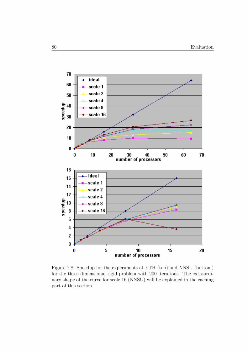
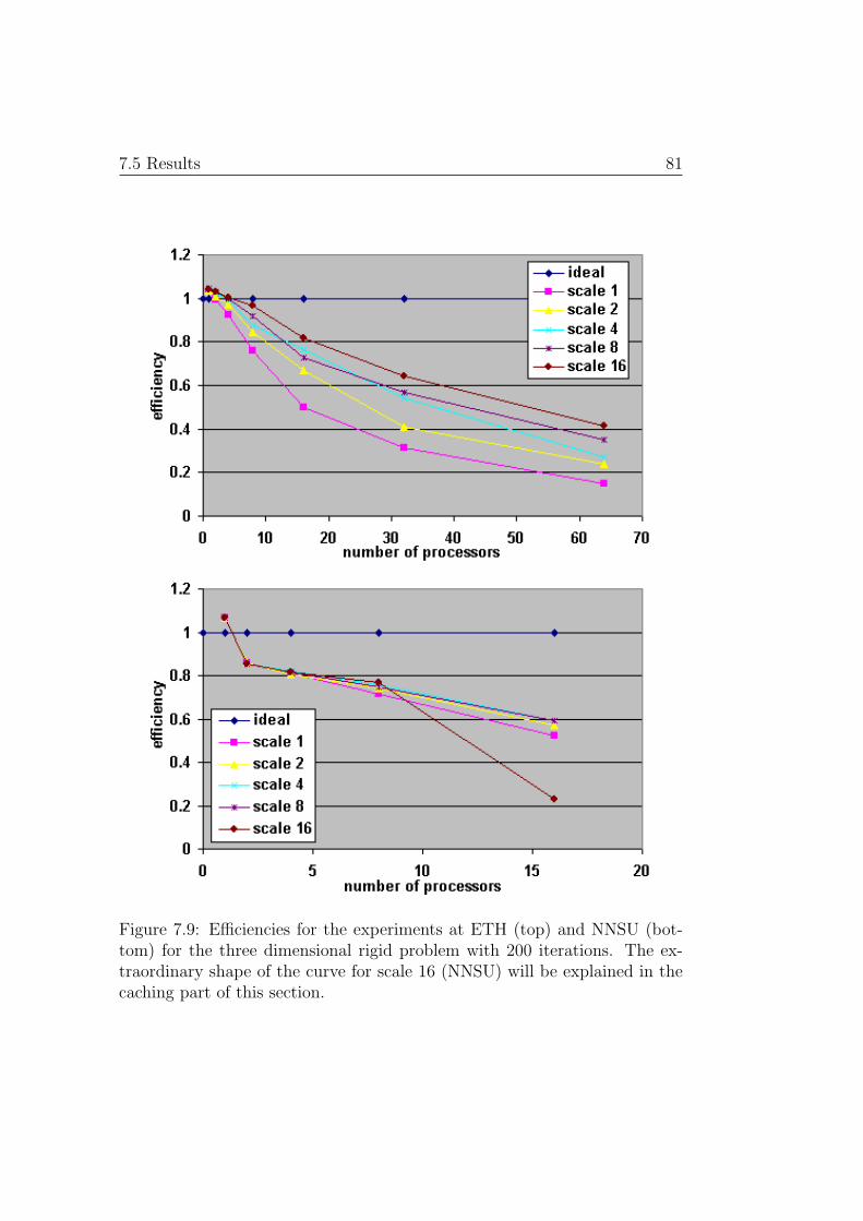
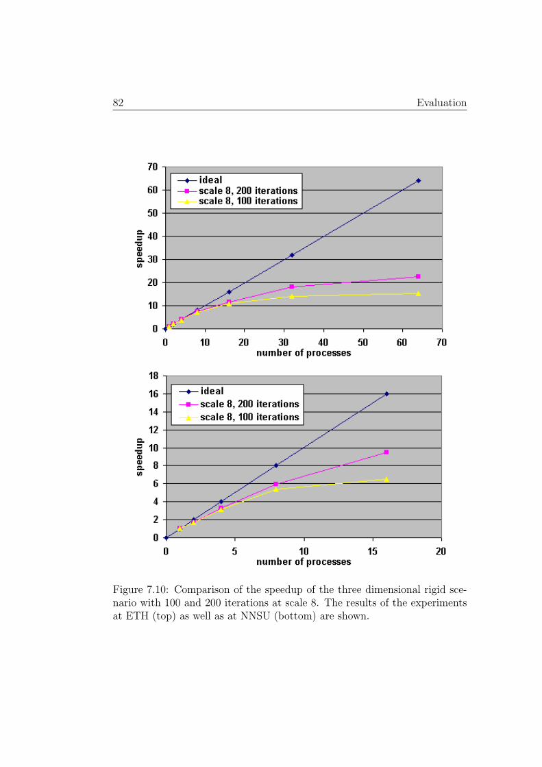
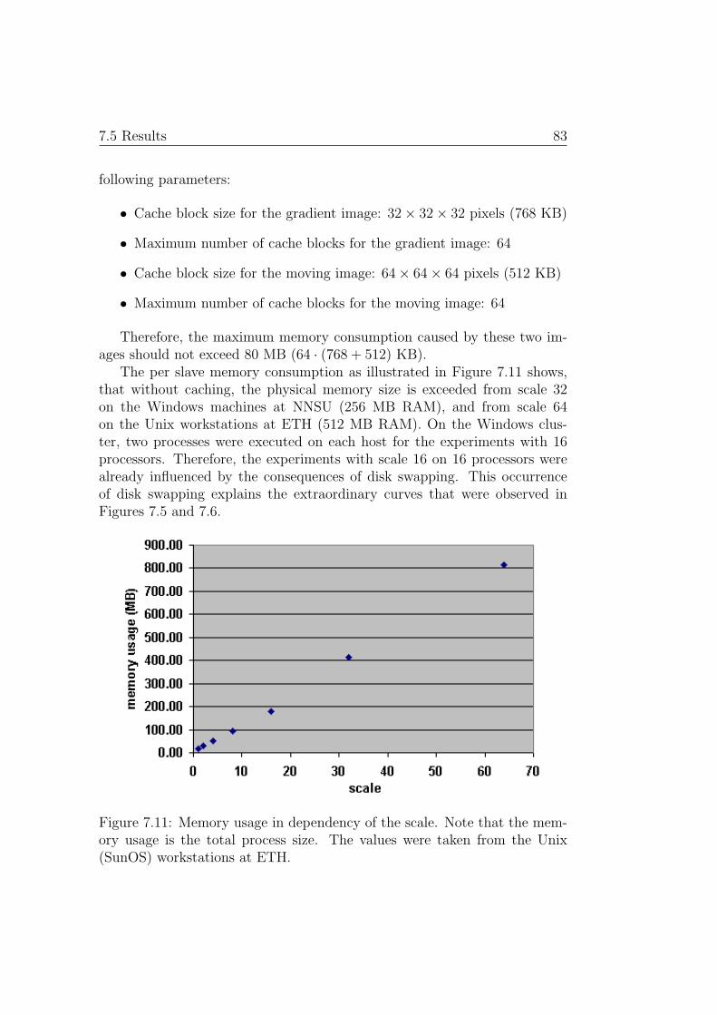
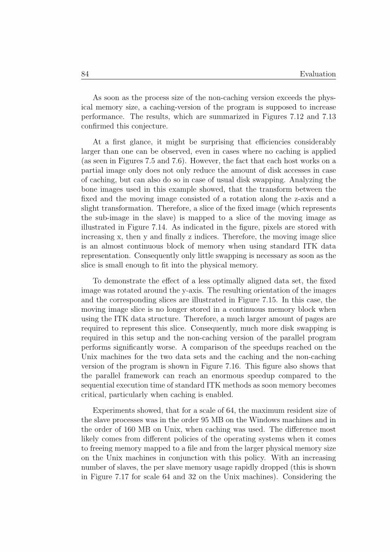
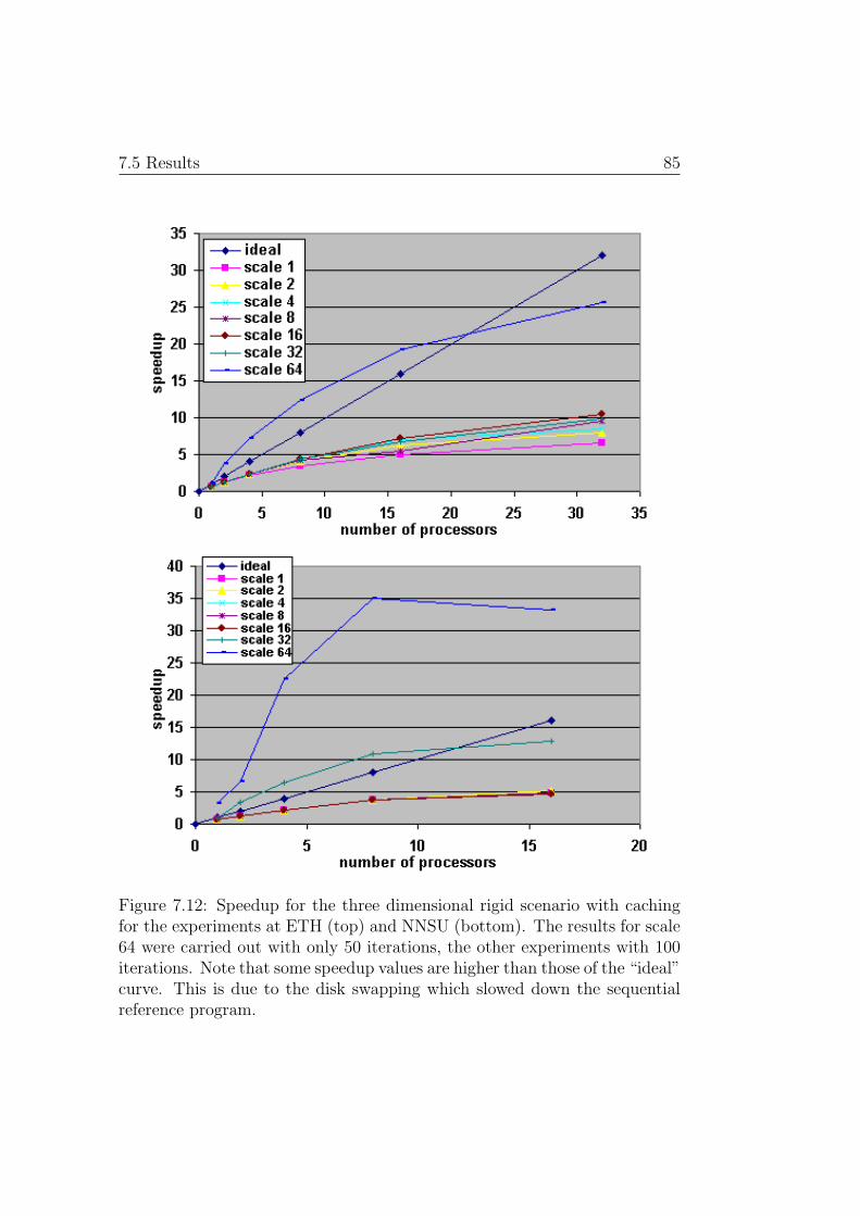
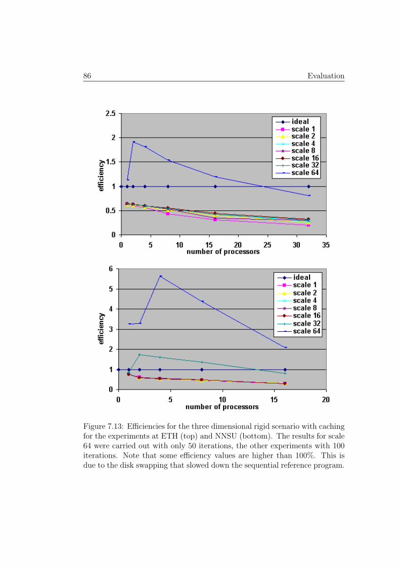
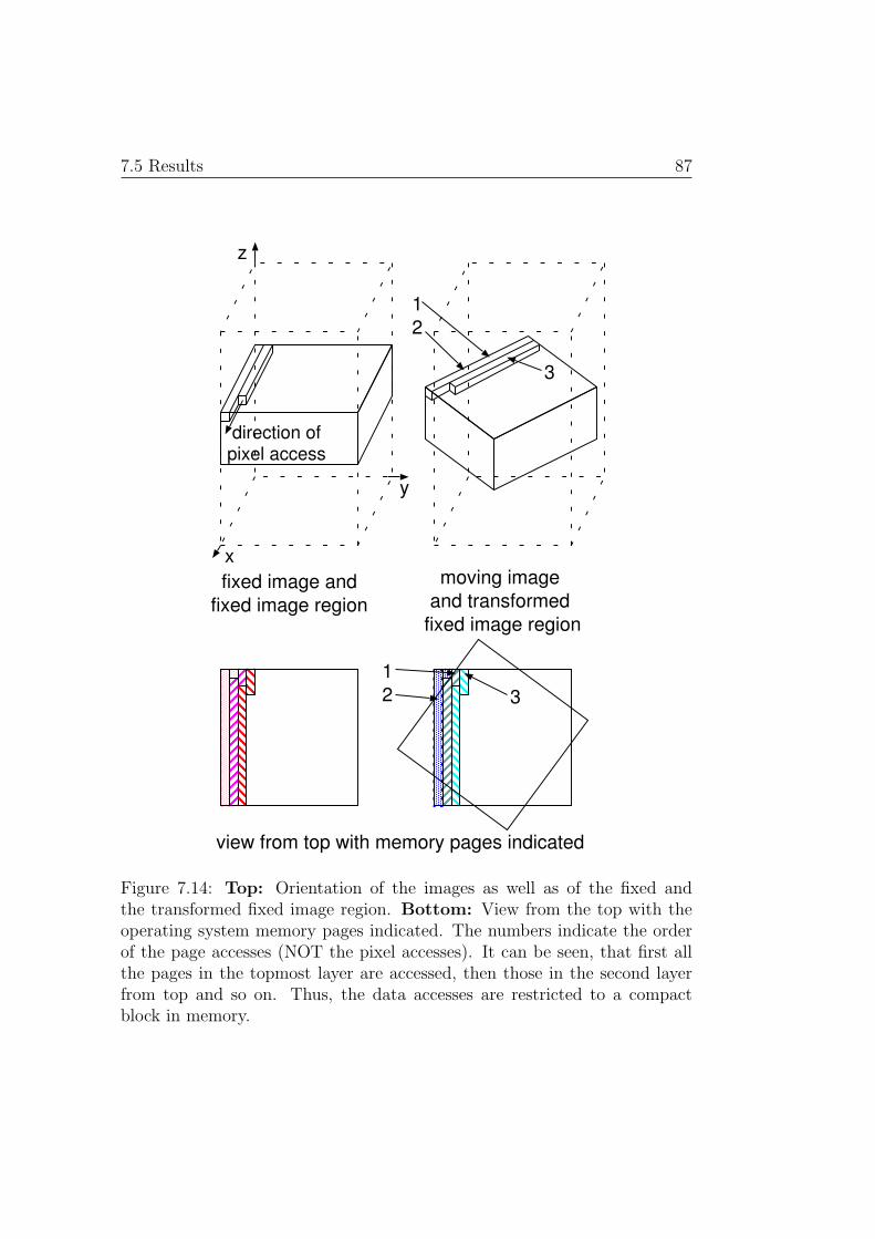
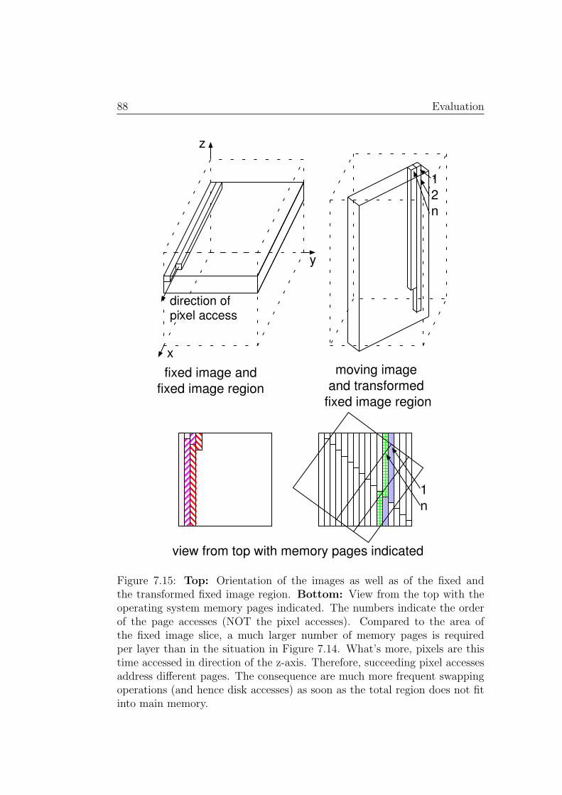
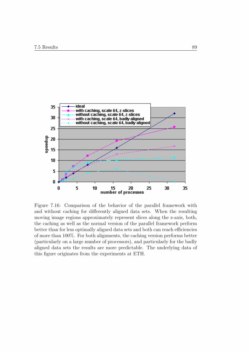
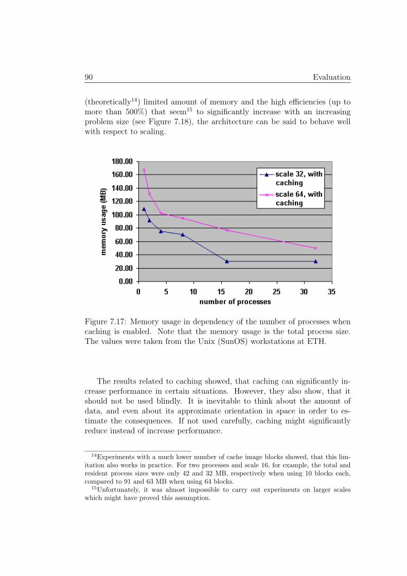
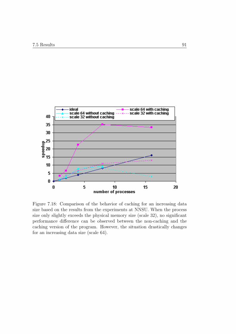
Image registration is the task of finding a spatial transformation that opti-mally maps one image onto another one. Thereby, usually a global optimumon a similarity function (metric) is searched. Out of the huge variety ofdifferent registration problems, many are computationally intensive and re-quire large amounts of memory. None of the most prevalent software librariesfor image registration provides parallel computing methods for distributedmemory environments, although the task has successfully been parallelizedin several projects. Therefore, this thesis addresses the extension of one ofthe most important libraries with a framework for parallel image registrationin distributed memory systems, such as clusters of workstations. The devel-oped framework is based on a distributed calculation of the metric function(as opposed to parallel optimization). The distribution is coordinated by ageneric module which serves as the basis for the parallelization of new met-ric functions and at the same time hides the parallelization details from theuser. Maximum flexibility with respect to the underlying hardware is en-sured by an abstract communication layer and a caching mechanism allowsto process even large images without exceeding the physical memory of theparticipating nodes. By interacting with the numerous components providedby the library, the framework can address a rich variety of different registra-tion problems, which is exemplarily demonstrated in three scenarios. Basedon these scenarios experiments have been carried out on different platforms.They show that in some cases a near linear speedup can be reached even on alarge number of processes despite of the generic character of the methods andthat the framework performs particularly well in data intensive applicationsbecause of the avoidance of disk swapping due to the combination of cachingand the accumulated memory capacity in a cluster.
In der Bildregistrierung (Image Registration) geht es darum, eine raumlicheTransformation zu finden, welche ein Bild optimal auf ein anderes abbildet.
iv Abstract
Dazu wird ublicherweise ein globales Optimum auf einer Vergleichsfunkti-on (Metrik) gesucht. Aus der grossen Auswahl verschiedener Registrierungs-probleme sind viele rechenaufwendig und haben einen grossen Speicherbe-darf. Keine der am weitesten verbreiteten Software Bibliotheken fur Bild-registrierung verfugt uber Parallel-Computing-Methoden fur Umgebungenmit verteiltem Speicher, obwohl das Problem in verschiedenen Projekten er-folgreich parallelisiert wurde. Deshalb widmet sich diese Arbeit der Erwei-terung einer der wichtigsten Bibliotheken mit einem Framework fur paral-lele Bildregistrierung fur Systeme mit verteiltem Speicher, wie zum BeispielWorkstation-Clusters. Das entwickelte Framework basiert auf einer verteil-ten Berechnung der Vergleichsfunktion (im Gegensatz zu paralleler Optimie-rung). Die Verteilung wird koordiniert durch ein generisches Modul, welchesals Basis fur die Parallelisierung neuer Metriken dient und gleichzeitig dieParallelisierungsdetails vor dem Benutzer verbirgt. Ein abstrakter Kommu-nikationslayer garantiert maximale Flexibilitat im Bezug auf die zu Grundeliegende Hardware-Architektur, und durch einen Caching-Mechanismus wirdes moglich, auch grosse Bilder zu bearbeiten ohne dabei die Arbeitsspeicher-Kapazitat der beteiligten Knoten zu ubersteigen. Die Interaktion mit denzahlreichen Komponenten, welche die Bibliothek zur Verfugung stellt, er-laubt den Einsatz des Framework in einer breiten Auswahl von Problemenim Gebiet der Bildregistrierung. Dies wird anhand dreier Beispiel-Szenariosexemplarisch demonstriert. Aufbauend auf diesen Szenarios wurden Experi-mente auf verschiedenen Plattformen durchgefuhrt. Diese zeigen, dass trotzdes generischen Charakters der Methoden in gewissen Fallen ein beinahelinearer Speedup erreicht werden kann, und dass das Framework in daten-intensiven Problemen besonders gute Ergebnisse erzielt. Dies, da durch eineKombination von Caching und der akkumulierten Speicherkapazitat einesClusters das in sequenziellen Programmen auftretende Disk-Swapping ver-mieden werden kann.
A.4 Organization of the Work . . . . . . . . . . . . . . . . . . . . 126
B Time Table 129
Bibliography 133
Index 138
viii CONTENTS
Chapter 1
Introduction
Image registration is the process of establishing a point-by-point correspon-dence between two images of a scene. The images can thereby be acquired bydifferent sensors or by the same sensor in different points in time or from adifferent point of view. Image registration is applied in several fields, such asin medical imaging, in stereo vision applications, for motion analysis, objectlocalization or image fusion.
The correspondence between the images is defined by a spatial transfor-mation, which is usually computed by an optimization process. Thereby anoptimizer searches a global optimum on a function which defines a similaritymeasure (metric function1) between the images dependent on their relativeposition.
For more profound information about image registration please refer toSection 2.1.
Different software packages, libraries and frameworks exist that carry outimage registration. Some of the most prevalent tools are the Automated Im-age Registration (AIR) package [1], the Flexible Image Registration Toolbox(FLIRT) [2], the VTK CISG Registration Toolkit [3], the Image ProcessingToolbox of Mathworks (for Matlab) and the Insight Segmentation and Reg-istration Toolkit (ITK) [4]. Among these projects, ITK is the most genericand extensive approach. Apart from the Image Processing Toolbox of Math-works, all the above mentioned packages are open source projects that arefreely available. However, only the Insight Segmentation and RegistrationToolkit can be used free of charge in commercial applications.
Dependent on the application, image registration can be a resource de-manding task. The main problems are the sometimes large amounts of data,
1the similarity function is often called metric function, even though it does not neces-sarily meet the definition of a metric in the mathematical sense
2 Introduction
that can easily exceed the physical memory size of a state of the art com-puter, as well as the search space, which can reach a considerable size2 in someproblems. Exploring large search spaces and data sets inherently causes longcomputing times. What makes things even worse is the fact, that for largeimages, computers can run out of available physical memory. The resultingdisk swapping causes a considerable increase in computing time.
Parallel computing has proven to be an efficient technique to solve both,memory and performance problems. Most specialists dealing with image reg-istration are not familiar with parallel and distributed computing techniques.To bridge the gap between specialists of different disciplines, Squyres et al.[5] as well as Seinstra and Koelma [6] propose to integrate parallel computingmethods into image processing libraries. Despite of the fact, that such meth-ods have successfully been applied to specific image registration problems,no generic software modules exist that address the image registration taskby means of parallel computing.
This thesis addresses the problem of parallelizing the image registrationtask and thereby tackles performance as well as memory issues. The goalwas to develop methods that act as generic modules which can be used ina multitude of registration problems. This should be achieved by extendingan existing library. To account for the diversity of the addressed registrationproblems the methods had to be designed for clusters of workstations (whichare cheap and highly available) rather than for dedicated parallel computers.
Parallelization methods for optimization tasks can be divided into coarseand fine grained. While in coarse grained methods multiple independentfunction evaluations are parallely executed, fine grained methods calculatethe basic computational steps in parallel. According to Eldred and Schimel[7], the parallel efficiency for coarse grained methods is usually better, andbest performance and scalability can be achieved by combining coarse andfine grained methods.
Applying this scheme to image registration shows that there are basicallytwo strategies: parallelizing the optimization method or parallelizing the met-ric function evaluation. These strategies can also be combined. Approachesbased on both, parallel optimization as well as parallel metric function eval-uation have successfully been realized before.
When applying coarse grained methods, memory issues still remain criti-cal, since each function evaluation requires the whole data set. Furthermore,coarse grained methods usually scale only within a limited range. Several
2For deformable problems, search spaces of up to 9.8 × 10⁶ parameters have beenreported. However, more typical are search spaces from about six to a few hundredparameters.
3
voxel based registration techniques are well suited for fine grained parallelcomputation based on parallel metric function evaluation. This thesis con-centrates on exactly these techniques.
A generic module for parallel metric computation has been developed,which extends the basic registration framework of the ITK library. Togetherwith the huge diversity of registration components within ITK, this moduleallows the use in a multitude of applications. A caching mechanism has beenintroduced that takes advantage of the fact that each processor works ona partial image only when parallely evaluating a metric function. Enablingthis mechanism allows to treat even large data size problems with a moderateamount of memory.
The developed methods have been integrated into three different scenariosand thereby successfully been tested for suitability in two and three dimen-sional, rigid and non-rigid as well as intra- and inter-modal registration. Ontwo different cluster systems, more that 1000 experiments have been carriedout. Thereby the speedup3 compared to the equivalent scenarios composedof standard ITK modules as well as scalability issues have been examined.The analysis of time spent in different parts of the code further allowed togain an insight into strengths and deficiencies of the developed framework.
It could be shown, that in some cases, a speedup of more than 15 can bereached on 16 and of over 50 on 64 processors. The use of caching, togetherwith the accumulated memory capacity of a cluster made it even possible toreach parallel efficiencies4 of far more than 100% compared to a sequentialprogram that causes the operating system to start disk swapping.
As a conclusion from these results, it can be said that the ITK library wassuccessfully extended by a generic framework for parallel image registration,which allows to treat even memory intensive problems.
The rest of this thesis is structured as follows:
Background: This chapter gives background information to image regis-tration, parallel computing and ITK and thereby introduces the mostimportant terms.
Related Work: The Related Work chapter first discusses the motivationof the project in more detail, based on work previously done in thearea. Then an overview of alternatives to parallel computing to addressthe performance and memory problems in image registration is given.Finally, other projects that address image processing and registrationby means of parallel computing are reviewed.
3See Section 2.2 for a definition.4See Section 2.2 for a definition.
4 Introduction
Problem Statement: The Problem statement chapter explains the prob-lem tackled by this thesis in detail.
Requirement Specification: This chapter defines the exact scope of thethesis. It covers requirements and restrictions on the support of reg-istration methods and the underlying hardware as well as an the ex-tendibility of the developed methods.
Distributed Registration Framework: The developed methods are pre-sented and explained in the Distributed Registration Framework chap-ter. Concepts as well as implementation are discussed in-depth. Areader that intends to use or extend the developed modules is stronglyencouraged to read this chapter.
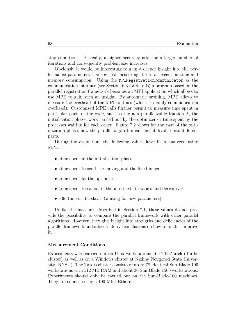
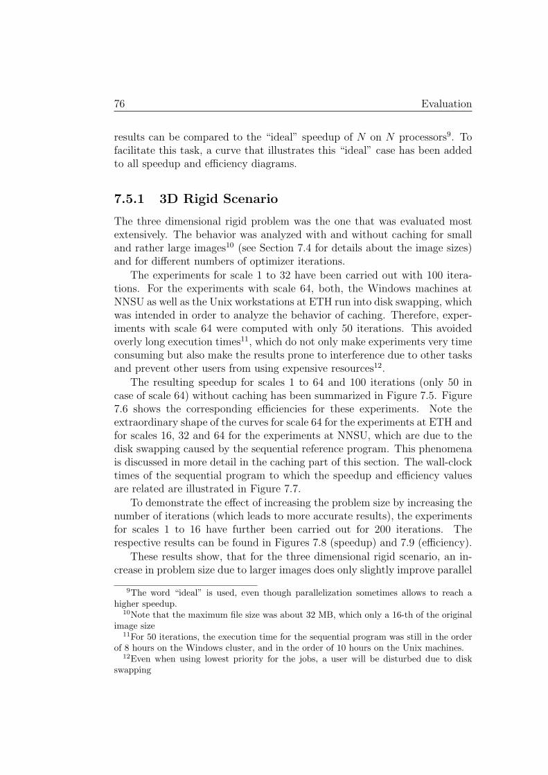
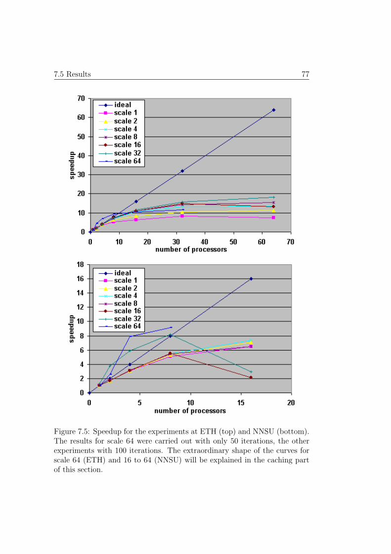
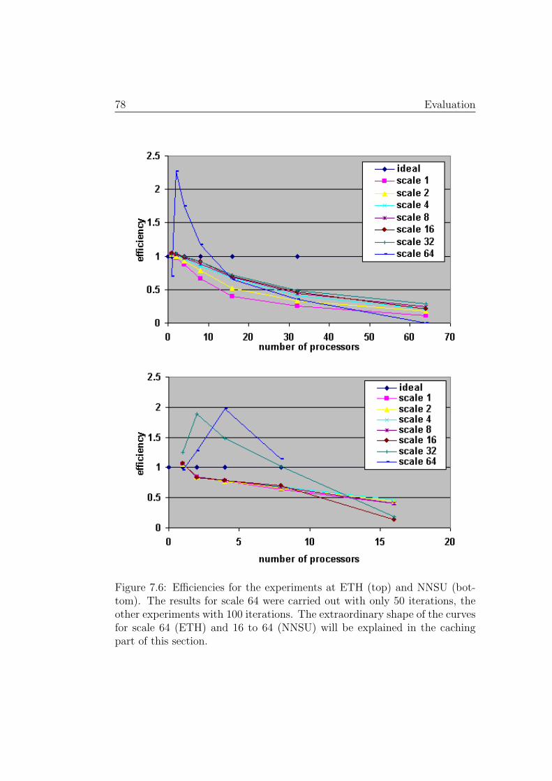
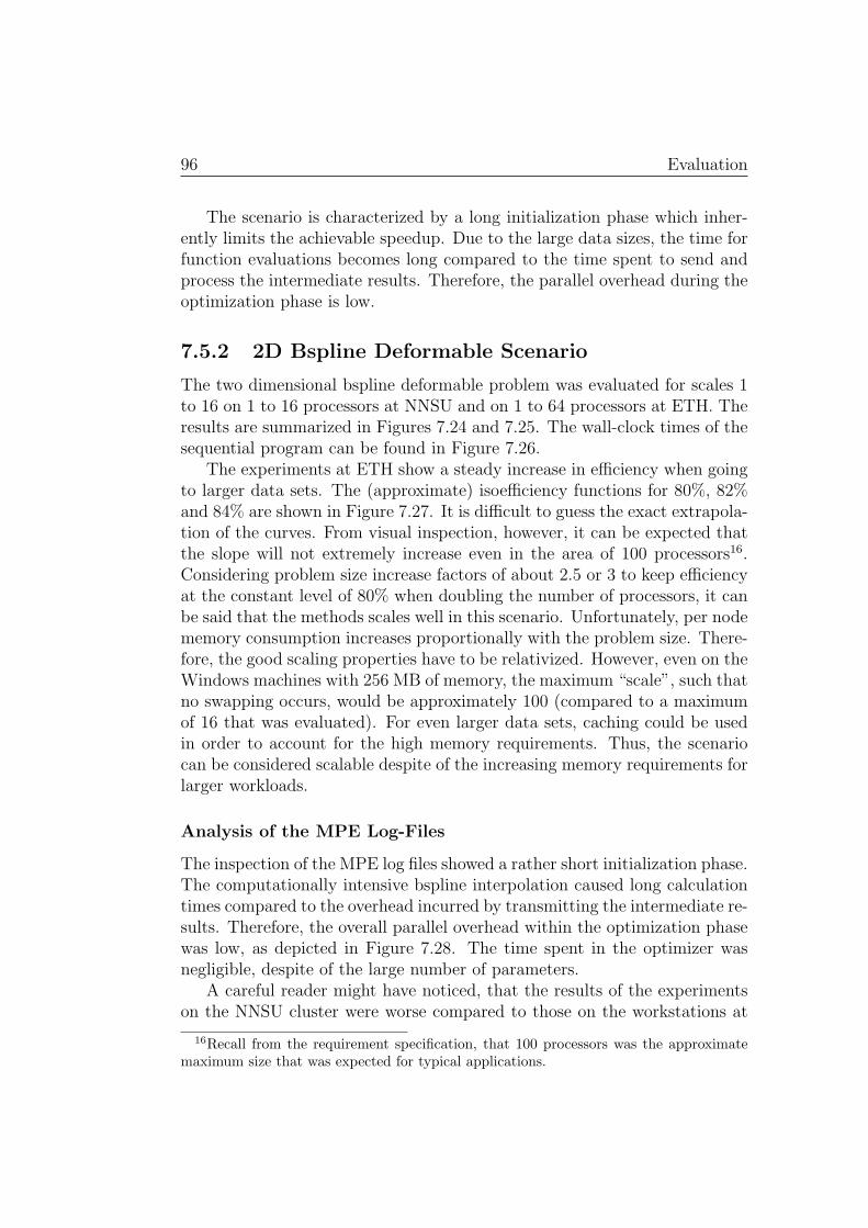
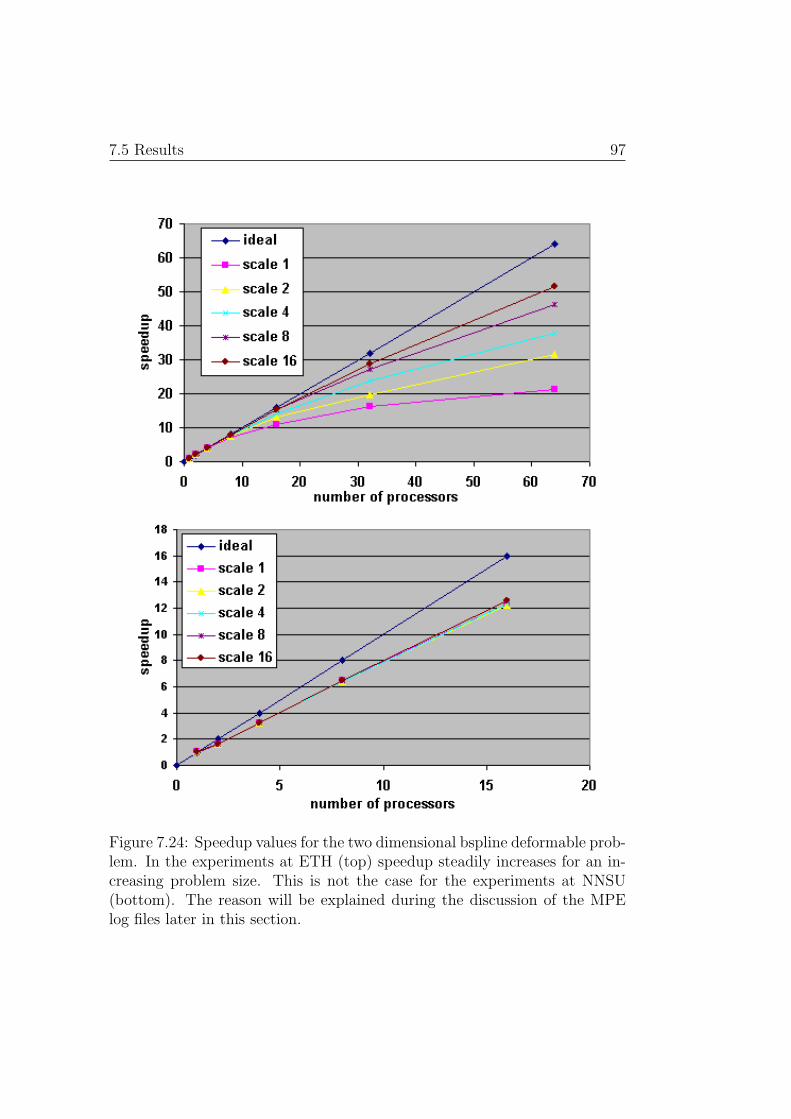
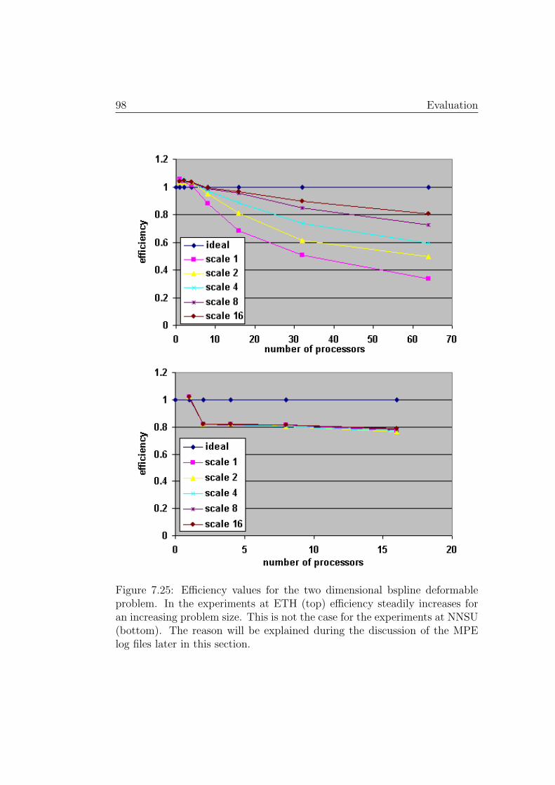
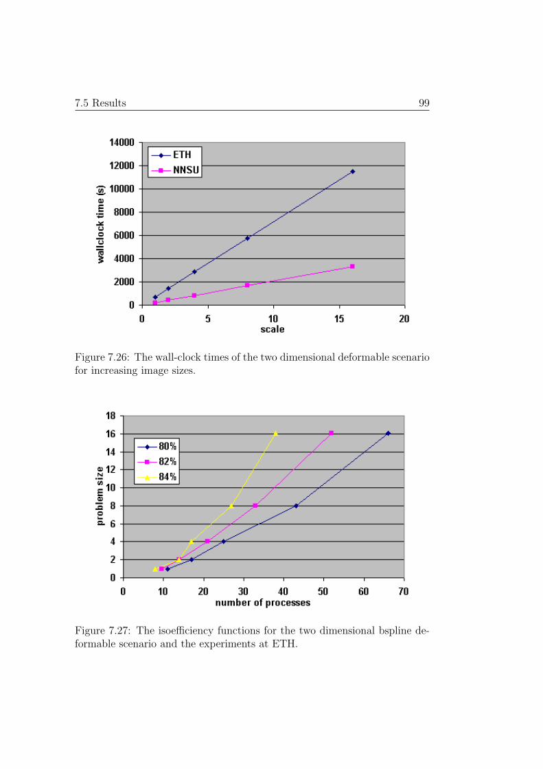
Evaluation: The Evaluation chapter discusses the methodology as well asthe results of the evaluation of the developed framework.
Future Work: This chapter outlines, how the framework can further beimproved.
Conclusion: The Conclusion chapter gives a concise review of what hasbeen reached by this thesis and what has been left over to futureprojects.
Chapter 2
Background
2.1 Image Registration
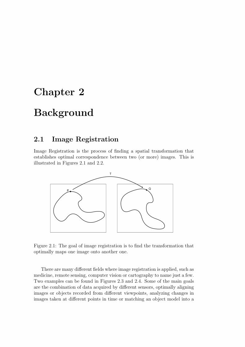
Image Registration is the process of finding a spatial transformation thatestablishes optimal correspondence between two (or more) images. This isillustrated in Figures 2.1 and 2.2.
P
T
Q
Figure 2.1: The goal of image registration is to find the transformation thatoptimally maps one image onto another one.
There are many different fields where image registration is applied, such asmedicine, remote sensing, computer vision or cartography to name just a few.Two examples can be found in Figures 2.3 and 2.4. Some of the main goalsare the combination of data acquired by different sensors, optimally aligningimages or objects recorded from different viewpoints, analyzing changes inimages taken at different points in time or matching an object model into a
6 Background
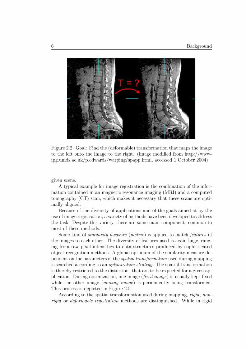
Figure 2.2: Goal: Find the (deformable) transformation that maps the imageto the left onto the image to the right. (image modified from http://www-ipg.umds.ac.uk/p.edwards/warping/spapp.html, accessed 1 October 2004)
given scene.A typical example for image registration is the combination of the infor-
mation contained in an magnetic resonance imaging (MRI) and a computedtomography (CT) scan, which makes it necessary that these scans are opti-mally aligned.
Because of the diversity of applications and of the goals aimed at by theuse of image registration, a variety of methods have been developed to addressthe task. Despite this variety, there are some main components common tomost of these methods.
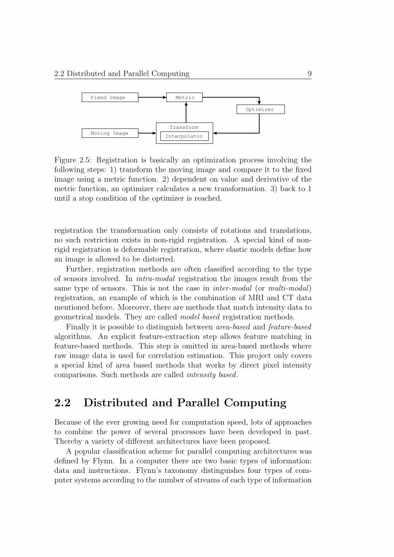
Some kind of similarity measure (metric) is applied to match features ofthe images to each other. The diversity of features used is again huge, rang-ing from raw pixel intensities to data structures produced by sophisticatedobject recognition methods. A global optimum of the similarity measure de-pendent on the parameters of the spatial transformation used during mappingis searched according to an optimization strategy. The spatial transformationis thereby restricted to the distortions that are to be expected for a given ap-plication. During optimization, one image (fixed image) is usually kept fixedwhile the other image (moving image) is permanently being transformed.This process is depicted in Figure 2.5.
According to the spatial transformation used during mapping, rigid , non-rigid or deformable registration methods are distinguished. While in rigid
2.1 Image Registration 7
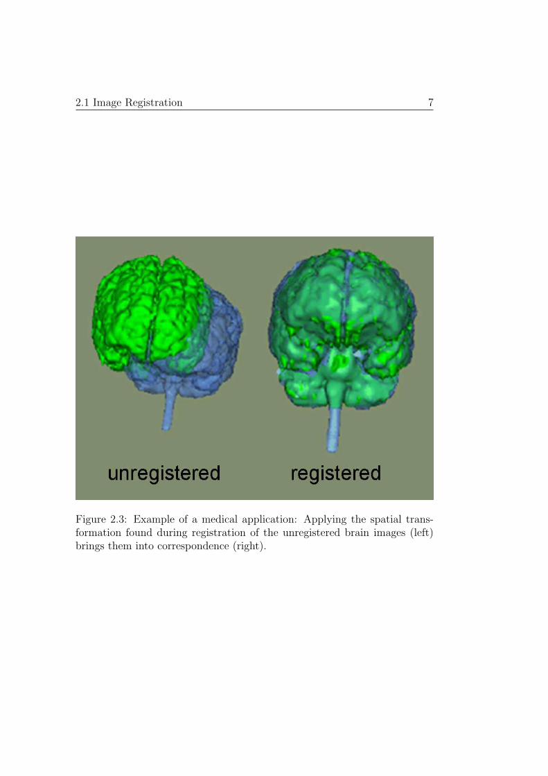
Figure 2.3: Example of a medical application: Applying the spatial trans-formation found during registration of the unregistered brain images (left)brings them into correspondence (right).
8 Background
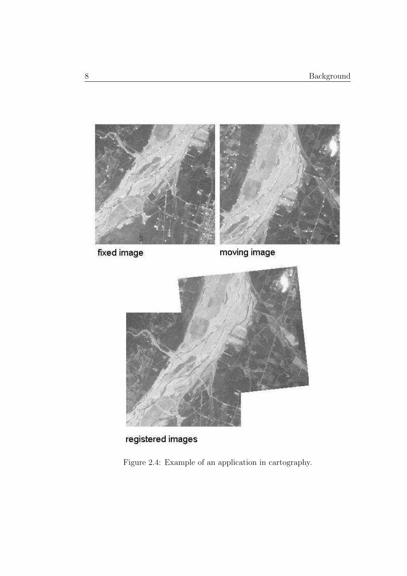
Figure 2.4: Example of an application in cartography.
2.2 Distributed and Parallel Computing 9
Fixed Image
Moving Image
Metric
Optimizer
Interpolator
Transform
Figure 2.5: Registration is basically an optimization process involving thefollowing steps: 1) transform the moving image and compare it to the fixedimage using a metric function. 2) dependent on value and derivative of themetric function, an optimizer calculates a new transformation. 3) back to 1until a stop condition of the optimizer is reached.
registration the transformation only consists of rotations and translations,no such restriction exists in non-rigid registration. A special kind of non-rigid registration is deformable registration, where elastic models define howan image is allowed to be distorted.
Further, registration methods are often classified according to the typeof sensors involved. In intra-modal registration the images result from thesame type of sensors. This is not the case in inter-modal (or multi-modal)registration, an example of which is the combination of MRI and CT datamentioned before. Moreover, there are methods that match intensity data togeometrical models. They are called model based registration methods.
Finally it is possible to distinguish between area-based and feature-basedalgorithms. An explicit feature-extraction step allows feature matching infeature-based methods. This step is omitted in area-based methods whereraw image data is used for correlation estimation. This project only coversa special kind of area based methods that works by direct pixel intensitycomparisons. Such methods are called intensity based .
2.2 Distributed and Parallel Computing
Because of the ever growing need for computation speed, lots of approachesto combine the power of several processors have been developed in past.Thereby a variety of different architectures have been proposed.
A popular classification scheme for parallel computing architectures wasdefined by Flynn. In a computer there are two basic types of information:data and instructions. Flynn’s taxonomy distinguishes four types of com-puter systems according to the number of streams of each type of information
10 Background
[8]:
• Single Instruction Single Data (SISD): these are usual sequential com-puters
• Multiple Instruction Single Data (MISD): such systems are rather un-usual, however there exist some kind of pipeline architectures that fitthis definition.
• Single Instruction Multiple Data (SIMD): a typical example for suchan architecture is a vector processor
• Multiple Instruction Multiple Data (MIMD): there are several systemsmatching this definition, a cluster of workstations for example.
Often the class of MIMD systems is further subdivided into shared mem-ory and distributed memory systems. In shared memory systems all proces-sors work on the same, shared address space. In distributed memory systems,on the other hand, each processor has assigned its own memory which otherprocessors cannot directly access. The most prevalent means of communica-tion in such systems is message passing.
Systems based on message passing often build up on libraries that takecare of the involved low level details, such as buffering, data type conversionin heterogeneous clusters or error handling. The most important librariesare the Parallel Virtual Machine (PVM) and different implementations ofthe Message Passing Interface (MPI) standard.
While Flynn’s taxonomy classifies parallel hardware architectures, thereis a similar scheme for parallel programming models. It distinguishes betweensingle program multiple data (SPMD) and multiple program multiple data(MPMD) programs. While in SPMD architectures the same program is runon every processing node, different pieces of software carry out the calculationin the MPMD case.
MPMD architectures are typical in applications where entirely differentcalculations have to be carried out on different nodes. Often, these calcu-lations are thereby applied to the same set of data. This kind of parallelarchitecture is also referred to task parallelism. SPMD programs are usuallyapplied when the same operations are applied to different parts of the data.This case is also referred to as data parallelism.
Often, one process slightly differs from the rest in the SPMD case. Thiscan be achieved by adding conditional statements that assign a special taskto the process with rank 0. The rank of a process is a unique identifier thatis assigned to each process. Usually, process ranks are integers that range
2.2 Distributed and Parallel Computing 11
from 0 to the n− 1 where n is the number of processes participating in thecalculation.
The methods developed throughout this project are designed for dis-tributed memory MIMD systems. The process with rank 0 has a specialtask assigned and the modules can be deployed in SPMD as well as MPMDprograms.
The quality of a parallel program is often measured in terms of two pa-rameters: parallel speedup and parallel efficiency . Parallel speedup is definedas
SN = TS/TN
where TS is the execution time of the best sequential algorithm1 and TN
is the execution time on N processors.Parallel efficiency is defined as
EN = SN/N
where N is the number of processors.An example should show the meaning of these measures: If the fastest
sequential algorithm executes in 8 seconds (TS = 8), and the parallel algo-rithm takes 2 seconds on 5 processors (N = 5, T5 = 2) we get a speedup S5
of 4. A speedup of 4 using 5 processors can be considered as an efficiency of80%, excatly as denoted by the measure E5.
There are different kinds of parallelization overhead that inherently limitspeedup. Often this overhead is due to the necessary interprocess commu-nication an is mainly characterized by the number and sizes of messages indistributed memory systems, and by synchronization issues in shared mem-ory systems. Further, parallel programs may perform poorly because of un-equally loaded nodes. Nodes might stay idle because they are waiting forothers to complete their task. Sophisticated load balancing algorithms wereproposed to handle this problem. Finally, there is limiting factor which isknown as Amdahl’s Law . Amdahl’s Law states that the maximum speedupthat can be reached by a parallel program is
S ≤ 1
f + (1− f)/N
1Note that it is difficult to define TS , because it is not clear which processor (a sin-gle processor in the parallel environment? the fastest available serial processor?) shouldbe taken as reference and because it is not generally possible to define the best sequen-tial algorithm because of several reasons such as memory versus performance trade-off,dependency on different problem properties or changes over time.
12 Background
where N is the number of processors and f is the non-parallelizable (andhence 1− f the parallelizable) fraction of the code [9]. This is a theoreticallimit, in practice this speedup will not be reached because of the paralleliza-tion overhead mentioned before.
Amdahl’s law can be modified to take into account the problem size W(which is basically the same as TS) as well as any overhead Tpo caused by theparallelization [10]:
SN =W
fW + (1− f)(W/N) + Tpo
=N
1 + (N − 1)f + NTpo
W
→ 1
f + Tpo
W
for N →∞
These equations show, that the non-parallelizable fraction, as well as theparallelization overhead should be minimized in order to achieve optimalspeedup.
2.3 ITK and its Architecture
The Insight Segmentation and Registration Toolkit (ITK) is an open-sourceimage processing library written in C++. It was designed to support theVisual Human Project [11] and mainly focuses on medical image segmen-tation and registration. ITK was developed by six principal organizationsand funded by the National Library of Medicine at the National Institutes ofHealth. However, many other organizations and individuals have been help-ing to evolve the software. Even though ITK is already a large package, it isstill rapidly growing. Reasons for that are the fact that ITK is open sourceand can be used free of charge even in commercial applications, as well asthe good support and documentation provided by the main developers.
Different technical features have been incorporated into ITK. These aremotivated by a design and implementation philosophy outlined in the ITKStyle Guide [12] and the ITK Readme [13]. The following sections are in-tended to give an overview of the most important architectural features.Some general design decisions are covered by Section 2.3.1. A discussionof the core feature of the ITK architecture, a pipeline mechanism for dataprocessing, follows in Section 2.3.2. Section 2.3.3 finally gives an overviewof the architecture of the basic registration framework within ITK. A de-
2.3 ITK and its Architecture 13
tailed overview of ITK and its concepts and classes can be found in the ITKSoftware Guide [4].
2.3.1 General Features
ITK is designed to be compilable on multiple platforms, that is on several im-portant C++ compilers and on different operating systems such as Windows,Unix or MacOSX.
To ensure a common build procedure on all platforms, CMake is used.CMake is a cross-platform build environment that allows to translate genericmakefiles into makefiles for a particular compiler.
Besides the support for different operating systems and compilers, ITKfurther provides bindings to other programming languages, namely TCL,Python, and Java.
To keep the algorithms and modules applicable to a large variety of differ-ent problems, ITK makes extensive use of generic programming techniques.To achieve high performance and at the same time keep the architecturegeneric, many modules are templatized, which allows to make decisions atcompile rather than at run time. The itk::Image class, for example, is tem-platized over the pixel type and the number of dimensions. In addition topixel-type images, other data representations such as point sets and meshesare supported. In a generic programming model, there are objects that store,and objects that operate on data. Objects that store data are also referredto as containers and objects that operate on it as algorithms. Often, a thirdclass of objects, the so called iterators are introduced. Iterators provide ageneric interface for algorithms to access data within containers and are animportant part of the programming model of ITK.
Another part of this programming model are the so called smart pointers ,which have been introduced because C++ does not take care about memoryallocation and freeing. Most objects within ITK are referenced by smartpointers that realize reference counting and automatically release memorythat is not used any longer. Further features are object factories, whichallow extensions of the system at run-time, a command-observer design pat-tern used for event handling and a pipeline architecture for data processing.This pipeline architecture is the core concept within ITK and it is thereforediscussed in more detail in the following section.
2.3.2 Pipeline Architecture and Data Streaming
Basically, two types of objects are involved in data processing: data objectssuch as images and meshes that represent data, and process objects that
14 Background
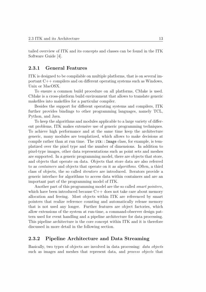
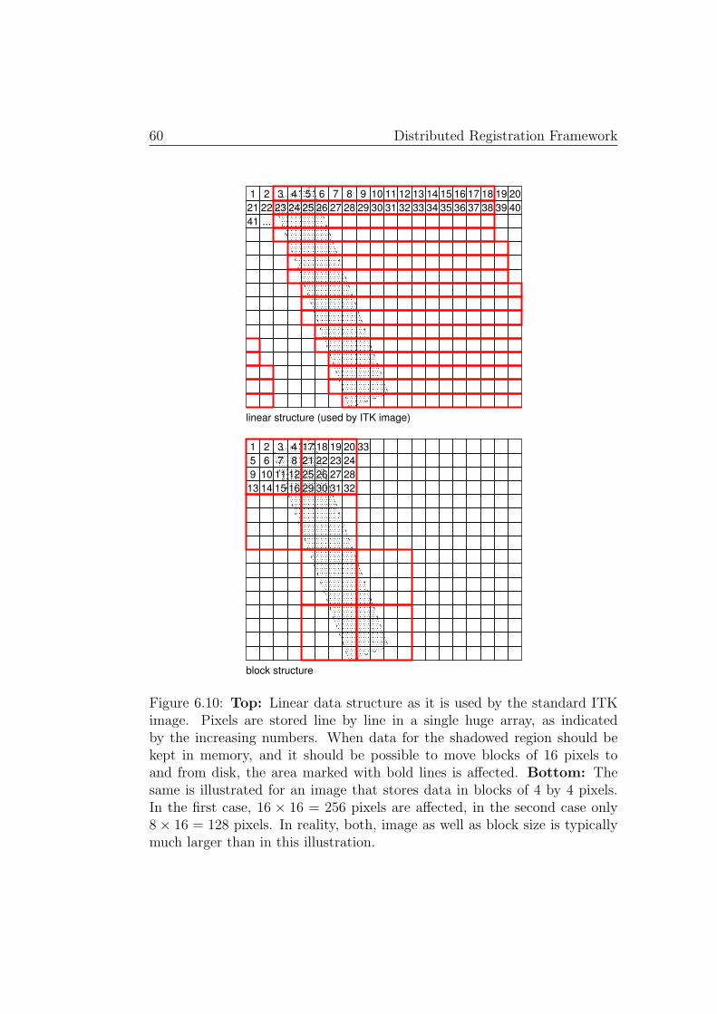
operate on data objects. These classes are connected by a data-flow pipelinemechanism as depicted in Figure 2.6. At the beginning of a pipeline, there isa process object usually referred to as source (a file-reader, for example). Itsoutput is an ITK data object. To this data object, another process object(a filter) is attached which again produces a data object and so on. Thepipeline is finally terminated by a so called mapper , a special process objectthat writes data to a file or any other output system.
...source dataobject filter filter data
object mapper
Figure 2.6: Illustration of the pipeline mechanism within ITK: process ob-jects are connected to data objects, which in turn are connected to otherprocess objects again.
This architecture does not only describe the flow of data, but also incor-porates some sophisticated concepts. It takes care of memory managementand makes sure the pipeline is always up to date while guaranteeing thatonly those sections are executed that have changed. It further enables datastreaming and multi threading (see below).
Within the pipeline, there is some trade off between memory efficiencyand execution speed. That is, once a filter has calculated its output, thisoutput can be kept in memory for re-usage, or the memory can be releasedand the filter has to re-execute if the output is needed again at a later pointin time. Therefore, each filter has a release data flag which optionally canbe set by the user. This allows to optimally adjust the pipeline behavior tothe application needs.
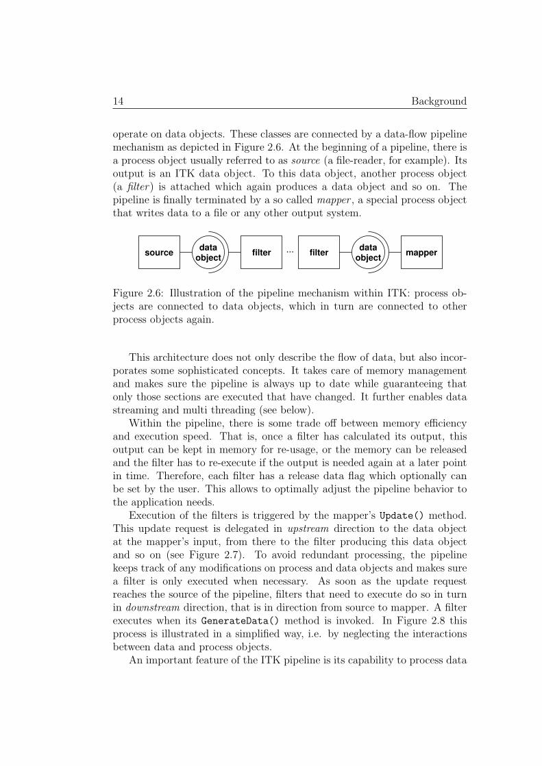
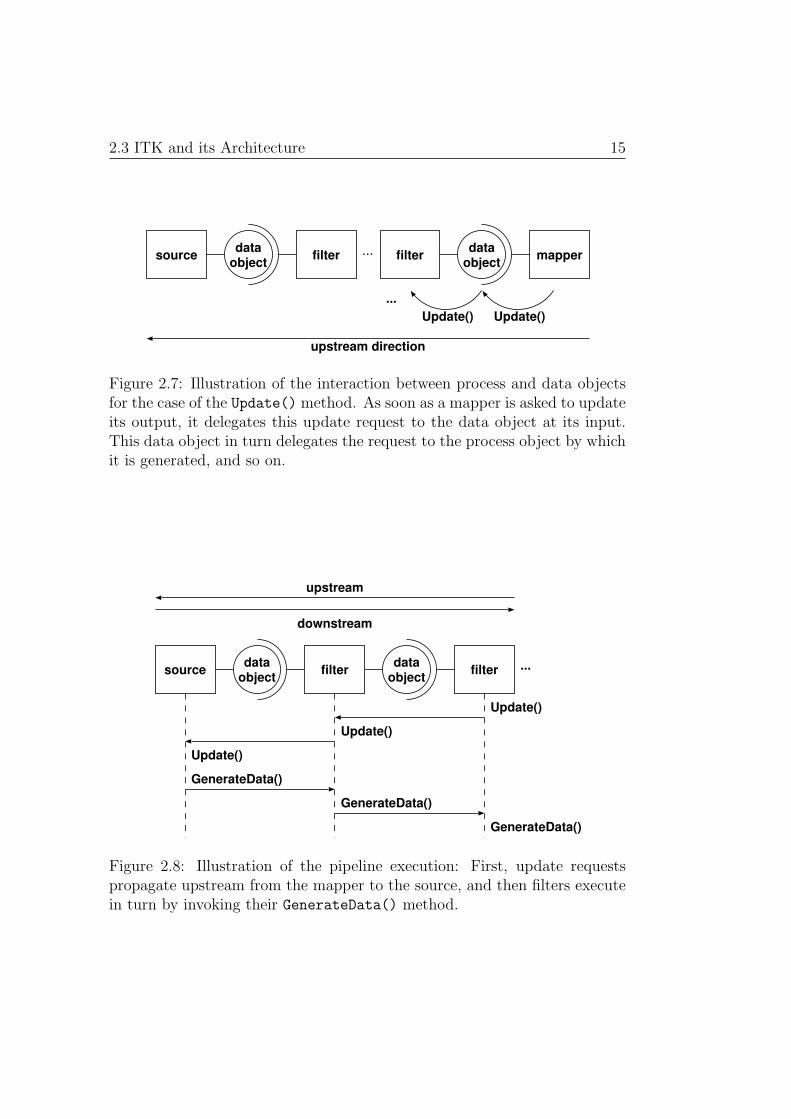
Execution of the filters is triggered by the mapper’s Update() method.This update request is delegated in upstream direction to the data objectat the mapper’s input, from there to the filter producing this data objectand so on (see Figure 2.7). To avoid redundant processing, the pipelinekeeps track of any modifications on process and data objects and makes surea filter is only executed when necessary. As soon as the update requestreaches the source of the pipeline, filters that need to execute do so in turnin downstream direction, that is in direction from source to mapper. A filterexecutes when its GenerateData() method is invoked. In Figure 2.8 thisprocess is illustrated in a simplified way, i.e. by neglecting the interactionsbetween data and process objects.
An important feature of the ITK pipeline is its capability to process data
2.3 ITK and its Architecture 15
...source dataobject filter filter data
object mapper
...Update() Update()
upstream direction
Figure 2.7: Illustration of the interaction between process and data objectsfor the case of the Update() method. As soon as a mapper is asked to updateits output, it delegates this update request to the data object at its input.This data object in turn delegates the request to the process object by whichit is generated, and so on.
source dataobject filter data
object filter ...
Update()
Update()
GenerateData()
GenerateData()
Update()
GenerateData()
upstream
downstream
Figure 2.8: Illustration of the pipeline execution: First, update requestspropagate upstream from the mapper to the source, and then filters executein turn by invoking their GenerateData() method.
16 Background
in pieces. This concept, which is named streaming , permits to apply thefilters within the pipeline on sub-images and to reassemble the whole imageat the end of the pipeline. Therefore, even very large images can be processedwithout exceeding physical memory size. Obviously, not every filter can beapplied to partial images, because of global data dependencies. Therefore,only parts of the toolkit are streaming capable. Even though some metricfunctions are suited to be applied to partial images, none of the registrationmethods within ITK supports streaming at the time of this writing.
Filters that support streaming are well suited for parallel computation.Therefore, they usually support multi-threaded execution. The basic con-cept, splitting data into pieces for processing, is the same. Thus, multi-threading comes at little cost when building up on the streaming architecture.A filter simply has to implement the ThreadedGenerateData() method in-stead of the GenerateData() method in order to be multi-threading capable.
The processing of sub-images is realized by a concept consisting of threedifferent image regions. These regions are the largest possible region, whichrepresents the entire dataset, the buffered region, which is a contiguous blockof memory allocated by filters to hold their output and the requested re-gion which is the part of the dataset that a filter is asked to process. AnImageRegionSplitter allows to divide the image region into several re-quested regions which are then processed one after the other.
The Update() method of data objects, invokes three methods:
• DataObject::UpdateOutputInformation()
• DataObject::PropagateRequestedRegion()
• DataObject::UpdateOutputData()
The output information consists of meta-data which allows to map thepixel coordinate system to a position in real world. It has to be changedwhen an image is shrunk, for example.
As indicated by its name, PropagateRequestedRegion() asks a preced-ing filter for an output of requested size. Sometimes a filter cannot satisfy thisrequest and produces a larger output. Further, a filter might need a largerregion at its input in order to generate its output. This occurs, for example,when some additional boundary pixels are required by a filter kernel.
The third method called by Update() is UpdateOutputData(), which de-termines whether a particular filter needs to execute. Once a filter executes,all filters downstream have to do so as well.
2.3 ITK and its Architecture 17
2.3.3 Basic Registration Framework
Since the multitude of registration problems asks for different methods tosolve them, ITK provides different registration frameworks, each suitable forsome particular applications.
There exist four registration frameworks within ITK, three of which areonly suited for specialized tasks. Two of these specialized frameworks treatdifferent deformable registration problems and the third makes model toimage registration2 possible. Besides these very specialized methods, a basicimage registration framework allows to solve a multitude of more generalregistration tasks. It provides intensity based algorithms for registrationproblems defined by global transforms as well as for some simple deformableproblems. This project only covers the basic registration framework, thearchitecture of which is discussed within this section.
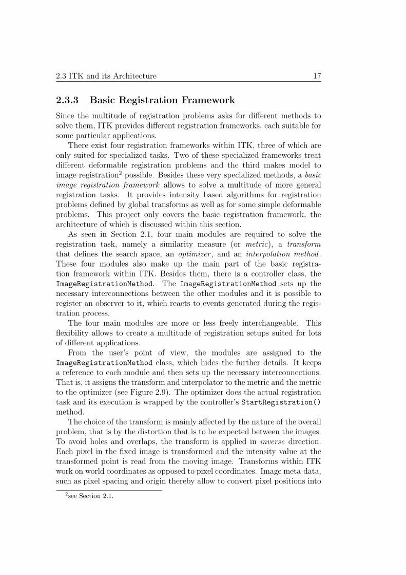
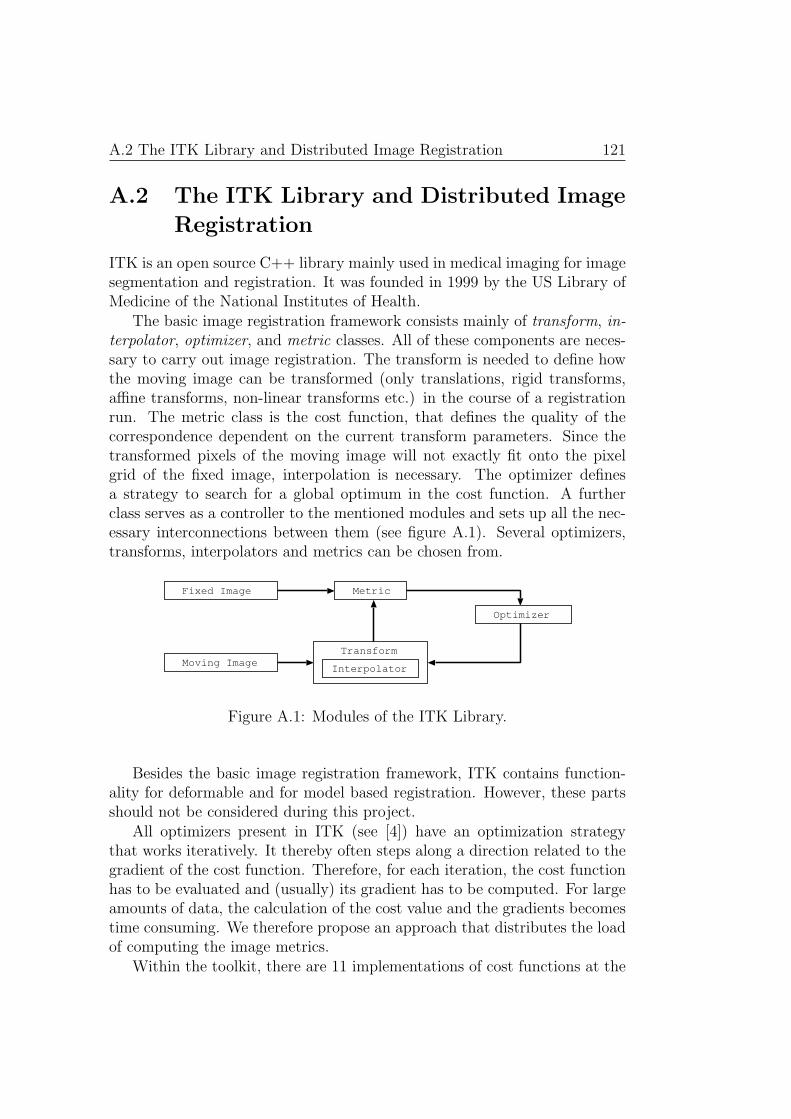
As seen in Section 2.1, four main modules are required to solve theregistration task, namely a similarity measure (or metric), a transformthat defines the search space, an optimizer , and an interpolation method .These four modules also make up the main part of the basic registra-tion framework within ITK. Besides them, there is a controller class, theImageRegistrationMethod. The ImageRegistrationMethod sets up thenecessary interconnections between the other modules and it is possible toregister an observer to it, which reacts to events generated during the regis-tration process.
The four main modules are more or less freely interchangeable. Thisflexibility allows to create a multitude of registration setups suited for lotsof different applications.
From the user’s point of view, the modules are assigned to theImageRegistrationMethod class, which hides the further details. It keepsa reference to each module and then sets up the necessary interconnections.That is, it assigns the transform and interpolator to the metric and the metricto the optimizer (see Figure 2.9). The optimizer does the actual registrationtask and its execution is wrapped by the controller’s StartRegistration()method.
The choice of the transform is mainly affected by the nature of the overallproblem, that is by the distortion that is to be expected between the images.To avoid holes and overlaps, the transform is applied in inverse direction.Each pixel in the fixed image is transformed and the intensity value at thetransformed point is read from the moving image. Transforms within ITKwork on world coordinates as opposed to pixel coordinates. Image meta-data,such as pixel spacing and origin thereby allow to convert pixel positions into
2see Section 2.1.
18 Background
ImageRegistrationMethod
Optimizer
Metric
Interpolator
Transform
Figure 2.9:
world coordinates. Using world coordinates for example guarantees that evennon-isotropic images are correctly treated.
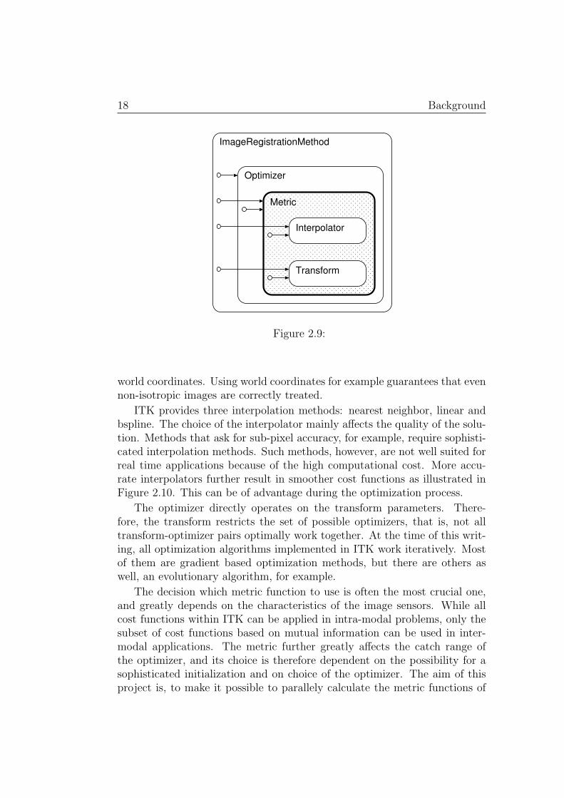
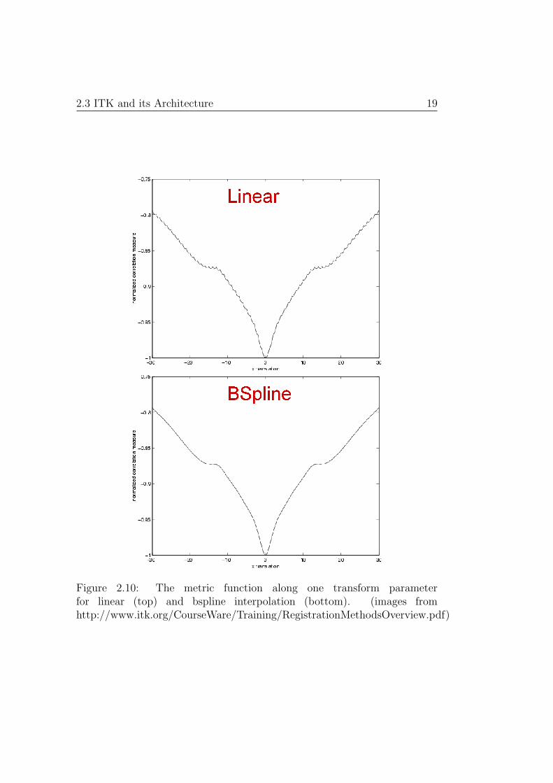
ITK provides three interpolation methods: nearest neighbor, linear andbspline. The choice of the interpolator mainly affects the quality of the solu-tion. Methods that ask for sub-pixel accuracy, for example, require sophisti-cated interpolation methods. Such methods, however, are not well suited forreal time applications because of the high computational cost. More accu-rate interpolators further result in smoother cost functions as illustrated inFigure 2.10. This can be of advantage during the optimization process.
The optimizer directly operates on the transform parameters. There-fore, the transform restricts the set of possible optimizers, that is, not alltransform-optimizer pairs optimally work together. At the time of this writ-ing, all optimization algorithms implemented in ITK work iteratively. Mostof them are gradient based optimization methods, but there are others aswell, an evolutionary algorithm, for example.
The decision which metric function to use is often the most crucial one,and greatly depends on the characteristics of the image sensors. While allcost functions within ITK can be applied in intra-modal problems, only thesubset of cost functions based on mutual information can be used in inter-modal applications. The metric further greatly affects the catch range ofthe optimizer, and its choice is therefore dependent on the possibility for asophisticated initialization and on choice of the optimizer. The aim of thisproject is, to make it possible to parallely calculate the metric functions of
2.3 ITK and its Architecture 19
Figure 2.10: The metric function along one transform parameterfor linear (top) and bspline interpolation (bottom). (images fromhttp://www.itk.org/CourseWare/Training/RegistrationMethodsOverview.pdf)
20 Background
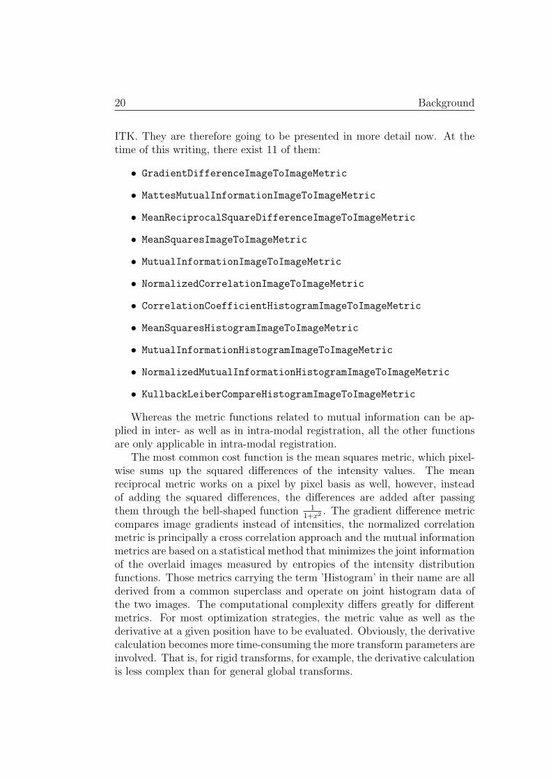
ITK. They are therefore going to be presented in more detail now. At thetime of this writing, there exist 11 of them:
Whereas the metric functions related to mutual information can be ap-plied in inter- as well as in intra-modal registration, all the other functionsare only applicable in intra-modal registration.
The most common cost function is the mean squares metric, which pixel-wise sums up the squared differences of the intensity values. The meanreciprocal metric works on a pixel by pixel basis as well, however, insteadof adding the squared differences, the differences are added after passingthem through the bell-shaped function 1
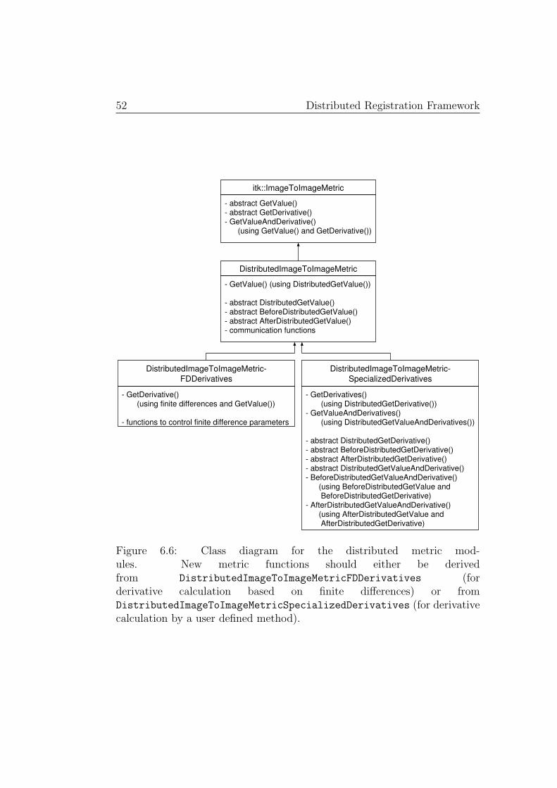
1+x2 . The gradient difference metriccompares image gradients instead of intensities, the normalized correlationmetric is principally a cross correlation approach and the mutual informationmetrics are based on a statistical method that minimizes the joint informationof the overlaid images measured by entropies of the intensity distributionfunctions. Those metrics carrying the term ’Histogram’ in their name are allderived from a common superclass and operate on joint histogram data ofthe two images. The computational complexity differs greatly for differentmetrics. For most optimization strategies, the metric value as well as thederivative at a given position have to be evaluated. Obviously, the derivativecalculation becomes more time-consuming the more transform parameters areinvolved. That is, for rigid transforms, for example, the derivative calculationis less complex than for general global transforms.
2.3 ITK and its Architecture 21
An extension of the basic image registration framework described aboveis the multi-resolution registration framework. It consists of the same basicmodules but operates on two so called image pyramids instead of two simpleimages as its input. An image pyramid represents an image at different res-olution levels. The framework takes care of all the necessary steps involvedwhen switching from one to the next resolution level. Multi-resolution reg-istration can considerably reduce computing time for large input images,and often the optimization process becomes more robust since there are lessundesired local optima for low resolution images (refer also to Section 3.2).
22 Background
Chapter 3
Related Work
3.1 Motivation
A huge diversity of different methods have been developed to address the im-age registration problem. Some of them demand for long calculation times.Dependent on the application, the main reasons for this computational ex-pense are the sometimes large image sizes [14, 15, 16], the large numberof parameters involved in the transform that creates a huge search space[15, 17] and the fact, that finding a global optimum on a highly non-linearmetric function is a complex task that asks for time consuming optimizationmethods [18, 19].
For registrations based on linear transformations, encountered executiontimes on a single processor on state of the art hardware at the respective timeof writing were 3-4 minutes for a resolution of 128×128×21 pixels [20] (1998),between 10 and 80 minutes for an image resolution of 125× 125× 250 pixels[16] (2003) and about 45 minutes for approximately 256 × 256 × 50 pixels[21] (1998). In deformable applications, the search space can be significantlylarger, which results in a considerable increase in computational complexity[15]. In such problems, computing times of up to 330 minutes were reportedby Rohlfing and Maurer [15] in 2003 and in 1996 Christensen et al. [17]stated that the calculation of a deformable registration problem with 9.8×10⁶
transform parameters on a 128 × 128 × 100 voxel volume can take up to 7days on a 150 MHz MIPS R4400.
Besides increasing the number of arithmetic operations, large data sizescan also cause problems with the memory constraints given by off-the-shelfcomputers [16, 21]. Image resolutions of more than 500×500×500 pixels arenot unusual in medical applications [16, 22]. Such images require storage inthe order of the available physical memory on a typical workstation computer.
24 Related Work
Exceeding physical memory causes disk swapping and therefore a drasticincrease in computing time. The problem of data size is likely to even increasein future, because of ever more data produced by ever better acquisitiondevices [14] and because of a trend from 2D to 3D image processing [21].
In some registration applications, long computing times are unacceptable.Among them are real time applications such as in range data analysis [23] orsensor fusion [24], applications that have to cope with the huge amount ofdata daily produced by a large amount sensors [14] and clinical applicationsthat ask for fast imaging in intra-operative situations as well as to cut downtime between scan and surgery [15, 21, 25].
Besides an enormously higher computing power, parallel computing canalso provide a solution to memory problems by using the aggregated memorycapacity provided by all nodes participating in the computation [14, 26, 27].This encourages the use of parallel computing in image registration appli-cations when performance is a problem. Since image processing experts areusually not quite familiar with parallel computing, different groups suggestedto hide the parallelization details of image processing tasks by the develop-ment of parallel image processing libraries, such as presented in [5], [28] and[6]. At the time of this writing, no such libraries exist that provide genericbuilding blocks for a multitude of registration applications in a distributedmemory parallel processing environment.
3.2 Alternative Approaches to Cut Down
Computing Time
Reducing execution time is an issue in image registration applications, andparallel computing is a possible solution to it, as outlined in the precedingsection. However, parallel computing asks for expensive resources. Thereforeit is a must to consider other alternatives that cut down computing timesprior to applying parallel computing methods. In image registration, thiscan be achieved by data as well as search space reduction [14].
Two main strategies are applied to reduce data sizes: Registration of sub-images only [14] and multi-resolution registration as applied in [14], [20] or[21]. The idea of the multi-resolution approach is to start at a low imageresolution to roughly approach the final solution and to successively refinethe image resolution to eventually reach the required accuracy.
Another idea to reduce data is the application of some kind of featureextraction prior to registration, instead of working on full pixel intensity val-ues. This, however, can lead to information loss which might be undesirable
3.3 Parallel and Distributed Computing in Image Processing andRegistration 25
in applications that ask for high accuracy [20].
The most important step in search space reduction is the applicationof an appropriate optimization method, that efficiently explores the searchspace. To avoid getting stuck in a local optimum on the metric function,often global optimization methods such as genetic algorithms are appliedas in [14], [18] or [19]. These methods, however, are usually more timeconsuming than local optimization methods [18, 19]. Another approach toavoid local optima is to provide an initial guess transform prior to applyinga local optimization method [16, 19, 21]. Finally, it is possible to rely onthe multi-resolution approach described above, which is more robust withrespect to getting trapped in a local optimum, since less of them exist at alow resolution level [20, 21].
Further search space reduction techniques can be found in deformableproblems. Examples are successive grid refinement [15] or compensation forglobal differences by applying a registration based on global transforms priorto the deformable registration [21].
All of these methods provide efficient ways to optimize image registrationperformance. However, they also show certain drawbacks. Data reductiontechniques such as sub-image registration or feature extraction might causeless accurate registration results and search space reduction techniques donot solve the memory problems caused by large data sets. The same holdsfor the multi-resolution approach as soon as it comes to working on the high-est resolution level. These drawbacks can be overcome by applying parallelcomputing methods.
3.3 Parallel and Distributed Computing in
Image Processing and Registration
Even though communication overhead is one of the most important reasonsthat limits the speedup of parallel applications, many authors state, thatimage processing tasks are good candidate for parallel computing because ofthe large data sizes involved [5, 9, 26, 27, 29, 30]. The inherent overhead ofdata distribution can only be overcome by parallel file system [5].
However, the fact that many image processing tasks are inherently parallel[5, 28, 31] often outweighs the problems caused by the data amounts andallows to achieve near linear speedup [5, 28]. Often, data parallelism isapplied to account for the localized operations in low level algorithms [9]and to cope with the involved data amounts [29]. Different strategies havebeen proposed to reduce transmission times of large amounts of data. These
26 Related Work
include using IP-Multicast [32, 33] for communication involving many nodesand compressing data prior to transmitting it, which sometimes allows toachieve an increased throughput. However this greatly depends on data andsystem properties [34, 35].
Image registration methods exhibit components that have some degreeof natural parallelism. Typically, either the optimization method or thecost function is parallelized. However, other approaches exist as well, suchas parallely calculating general matrix operations [24], solving differentialequations [17] or decomposing wavelets [36].
Among optimization methods, the most popular candidates for paral-lelization are evolutionary algorithms, as applied in [14], [18] and [19]. Themain reason for this popularity is the inherent parallel character of such al-gorithms as pointed out by Salomon et al. [19]. However, other optimizationmethods, such as the simplex algorithm, have successfully been parallelizedas well [15].
Many intensity based cost functions work on a pixel-by-pixel basis, ex-actly as typical low level image algorithms do. Approaches that take advan-tage of this inherently parallel nature of metric functions are presented in[15], [21], [23] and [25].
Eldred and Schimel [7] discuss the problem of parallel optimization froma more theoretical point of view. To avoid the scaling problems of paralleloptimization methods and at the same time taking advantage of their parallelnature, a combination with parallel function evaluation is proposed. Thisapproach has been applied to image registration by Rohlfing and Maurer[15] by combining parallel optimization with parallel metric calculation.
Parallel image processing has been deployed on different hardware archi-tectures. While some of them take advantage of the high number of process-ing units in an SIMD system [17, 24, 36], others trust in the higher flexibilityof dedicated MIMD architectures [15, 19, 21]. Further, several approachesbuild upon clusters of workstations [14, 18, 23, 25, 39, 40]. These systemsusually provide less computing power than dedicated architectures, howevertheir low cost, the high availability and the simplicity of adding further nodesoutweigh this disadvantage in many applications [37].
According to Fleury et al. [38], shared memory systems are better suitedfor image processing applications because they avoid excessive memory tomemory movements, and Downton and Crooks [9] state, that, while sharedmemory systems have successfully been applied in practice, there are prob-lems in reaching real-time performance with clusters of workstations. Otherexamples however show, that cluster and grid computing can be an alterna-tive to shared memory systems [5, 14, 18, 23, 25, 28, 29, 30, 39, 40]. Con-sidering future trends, the authors of [9] state, that MIMD systems built
3.3 Parallel and Distributed Computing in Image Processing andRegistration 27
from common microprocessors are likely to rule out dedicated parallel pro-cessors and they expect a trend towards switch based networks (as opposed topoint-to-point interconnections) and towards topology independent parallelalgorithms.
28 Related Work
Chapter 4
Problem Statement
As shown in Section 3.1, there are several factors that can cause image regis-tration to take more computing time than desired for a particular application.The most important factors are the large data sizes and search spaces. Eventhough there are several methods that reduce computing times on single pro-cessor systems, there are applications where it makes sense to use parallelcomputing methods. The main reasons that speak in favor of parallel com-puting are memory issues and the often inherent parallel character of theproblem.
The goal of this project is to speed up the image registration task bymeans of parallel computing methods in a distributed memory environment.Generic methods applicable in various applications should be developed in away that they are available to a wide audience. Thereby particular attentionshould be paid to applications involving large amounts of data.
The methods have to be integrated into the basic image registrationframework of ITK (see Section 2.3). That way, it is ensured that the re-sulting framework is generally applicable and available to a wide range ofusers. The implementation finally has to be investigated with respect toperformance and scalability.
As seen before, there are two main strategies to parallelize the image reg-istration task: Parallelizing the optimization method or parallelizing the costfunction evaluation. When applying parallel optimization, each processingnode requires a full copy of each, the fixed and the moving image. Theseimages have to be distributed as well as stored in main memory. When,on the other hand, the load of calculating the cost function is distributed,each processing node typically works on a partial image only. Therefore, inprinciple only one copy of each, the fixed and the moving image has to bedistributed and only partial images have to be kept in memory at each pro-cessing node. Efficiently coping with large data sizes is a main goal of this
30 Problem Statement
project. Therefore, the developed methods should be based on distributedmetric calculation rather than parallel optimization. Further, only intensitybased metric functions has to be considered. Such functions are usually wellsuited for parallelization as shown in Section 3.3.
Despite of the advantageous characteristics of parallel metric calculationwhen large data sizes are involved, network traffic and memory issues arestill likely to become a serious problem. These issues have to be consideredparticularly carefully and sophisticated data management techniques shouldbe incorporated if necessary.
To achieve the outlined goals, the project is organized in the followingfour major subtasks:
• specification of the detailed requirements of the implemented software(functional specification),
• design of an architecture for distributed image registration that fits intothe existing toolkit (ITK),
• implementation of the proposed architecture,
• investigation of the performance increase and the scalability.
Each of these subtasks is going to be discussed separately in the followingsections.
4.1 Requirement Specification
First, a requirement specification with a clear interaction and service modelhas to be defined. This model is the foundation for identifying the possibili-ties for parallelization and distribution and helps to delimit the scope of thethesis. The requirement specification should enfold the set of registrationproblems that has to be covered by the developed methods. Further it hasto define the requirements on scalability, on the amount and kind of datathat has to be supported and on hardware properties such as constraints onheterogeneous computer systems differing in processing power and memory,or on constraints and requirements of the communication subsystem.
4.2 Architecture Design
An architecture for distributed image registration based on parallel metriccalculation that fits smoothly into the existing part of ITK has to be designed.
4.3 Implementation 31
Thereby the overall architecture of the toolkit should be taken into account,allowing flexible extensions of the proposed architecture in future. Suchan extension could be the combination of the distributed metric calculationwith parallel optimization or the development of further distributed costfunctions. Besides pure computational speedup, the architecture should takeinto account memory issues and network traffic.
The design of such an architecture involves the following steps:
• studying the architecture of ITK and the characteristics of all costfunctions used in the basic image registration framework of the toolkit.Methods only applied in deformable and model based registrationshould only roughly be looked at, keeping future extensions in mind.The cost functions should mainly be investigated with respect to theirfeasibility for parallel calculation (local vs. global data dependencies)and with respect to their relations to other methods within the toolkit.Such relations can be similar mathematical characteristics as well asrelations within C++ (inheritance).
• based on above investigation of ITK as well as the previously definedrequirements, a design should be specified that exactly states whichparts of ITK should be implemented in a distributed manner and howthis should be done.
• above design should be refined by stating how to deal with issues con-cerning the underlying hardware as they are to be expected accordingto the requirement specification. Particular attention should be paidto data management issues.
• based on these considerations an architecture has to be proposed thataddresses all issues discussed before.
4.3 Implementation
Even though making the code official part of ITK is not the goal of thisproject, it should be written such that an integration can be achieved at alater point in time. Therefore, the code should be written with the ITKStyle Guide in mind, and tests on different platforms, as they are supportedby ITK, should be carried out during the implementation process. The re-quirements and restrictions of ITK should also be considered when choosinga particular interprocess communication infrastructure.
32 Problem Statement
4.4 Evaluation
The implemented architecture has to be investigated with respect to scala-bility and parallel efficiency for scenarios that cover the previously definedrequirements. Memory consumption as well as computation time should beconsidered theoretically as well as in experiments.
A sophisticated methodology has to be thought of that allows to quan-titatively assess the implementation. This methodology should define whichparts are evaluated, to what they are compared and how the measurementsare carried out.
Chapter 5
Requirement Specification
5.1 Image Registration Methods
The existing approaches to parallel image registration, as presented in Section3.3, all focus on particular problems. None of them provides the flexibilityto solve a wide variety of different registration tasks. To create such a flex-ible parallel image registration toolkit is exactly what this project aims at.The idea is to extend a widely used image registration library, the InsightSegmentation and Registration Toolkit (ITK), with parallel computing meth-ods. ITK is mainly thought for and used in medical applications, howeverits generic architecture allows the use in other fields as well.
As shown in Section 2.3.3, there exist several registration frameworkswithin ITK. During this project only the most generally applicable of them,the basic image registration framework, has to be extended. Further, onlythe load of calculating intensity based metric functions is addressed by thisproject, as stated in Section 4.
The characteristics of such functions are quite diverse. While some ofthem have local data dependencies only, others work on intermediate repre-sentations gathered from the whole image. The architecture of the methodsdeveloped throughout this project have to cover all of them.
To ensure maximum flexibility of the resulting framework, any of thefurther components required in image registration, namely transform, inter-polator and optimizer, have to be supported by the distributed methods.Particular attention should be paid to those components that cause highcomputational complexity.
It is important to note that the methods mentioned before need to becovered only by the design. Not all configurations have to be evaluated, andmainly in the case of metric functions, not all of them have to be imple-
34 Requirement Specification
mented. In a first step, a prove of concept implementation with a simplecost function, such as the mean squares metric, should be realized. Then,a metric function applicable in inter-modal registration problems, i.e. onebased on mutual information, can be parallelized.
5.2 Distributed Architectures
It cannot be expected that there is dedicated parallel hardware around intypical (i.e. medical) application fields of ITK. One option to overcome thisproblem is by remote access to high performance computers. However, thisis typically expensive and makes dependent from the provider of the system.As mentioned in Section 3.3, cluster computing can provide a powerful andaffordable alternative to dedicated parallel hardware. Therefore, the targetenvironment on which the extended library should be applicable are clustersof workstations. Typical cluster sizes might range from a few, say three orfour, computers within a laboratory in a hospital up to a hundred and morenodes in research labs. Any of these clusters should be supported by thearchitecture. Because of the typically large amounts of data involved, a fastnetwork (100 Mbps and more) will be indispensable and can be considereda prerequisite during architecture design. As a topology, a datagram basednetwork is assumed, which virtually connects all nodes to each other andwhich uses the IP protocol to address them. Further, it can be expectedthat the nodes within the cluster are located close to each other, that is inthe same building or complex, which results in low network delays. It isassumed that TCP is used at the transport layer, which leads to reliablecommunication links.
Unfortunately, clusters of workstations have the disadvantage of un-equally loaded nodes, as seen in Section 3.3. For an effective operationin a real world application, sophisticated load-balancing algorithms there-fore have to be provided. In a first step only a simple static load balancingscheme needs to be implemented. This assumes identical workstations withinthe cluster that are equally loaded at any time. However, the architectureshould be designed such, that the extension with advanced dynamic load bal-ancing methods is possible in future. This allows the use in heterogeneousclusters with unequally loaded nodes.
5.3 Requirements on Data to be Processed 35
5.3 Requirements on Data to be Processed
The diversity of typical applications of ITK asks for different image types andmethods, such as 2D rigid or 3D deformable registration. The parallel frame-work is supposed to cover the same types of data as the basic registrationframework of ITK.
As mentioned before, parallel computing is usually interesting where largevolumes of data are involved. Therefore, images that contain up to severalhundred millions of pixels (and hence require several hundred megabytes forstorage) have to be processable.
As shown in Section 3.3, data compression prior to transmission over anetwork can increase overall throughput. This, however, greatly dependson the data involved and on the underlying network. Therefore the archi-tecture should allow to add compression methods developed for particularapplications and particular data in future.
5.4 Requirements on Extensibility
ITK is a rapidly evolving library. Therefore, it is essential to keep the archi-tecture flexible, allowing extensions in future.
As mentioned earlier, the architecture has to be designed such that metricfunctions added to the toolkit in future can profit from the parallel computingmethods developed throughout this project. This will in general not bepossible without extra work, but the additional effort required to integrate anew function into the distributed framework should be as low as possible.
It would be interesting to design the architecture such that support formulti-threading, as it is provided by other ITK methods, can be added atlittle cost in future. That way, shared memory systems could easily takeadvantage of the developed methods.
5.5 Summary
5.5.1 Image Registration Methods
Supported by the Architecture
• only intensity based methods
• only the load of calculating the metric functions needs to be parallelized
• only the basic image registration framework
36 Requirement Specification
• all metric functions within the basic registration framework
• all transformation methods within the basic registration framework
• all optimization strategies within the basic registration framework
• all interpolation methods within the basic registration framework
Covered by the Implementation
• at least one typical metric function has to be parallelized
• several combinations of modules should be tested
5.5.2 Distributed Architectures
Supported by the Architecture
• clusters of workstations
– from 3 to 100 hosts
– connected by a switched network allowing a throughput of100 Mbps and more
– using the IP protocol to address hosts
– hosts located not far from each other
– reliable communication links (assuming TCP as transport proto-col)
– unequal processing power and load
Covered by the Implementation
Experiments have to be carried out on at least one typical cluster accordingto the description above. Only a static load balancing scheme has to beimplemented, i.e. processing power and load can assumed to be identical forall hosts.
5.5.3 Requirements on Data to be Processed
Covered by the Architecture
• 2 and 3 dimensional data
• large images (several hundred millions of pixels)
5.5 Summary 37
• use of the streaming capabilities of the toolkit to process large data
• possibility to preprocess data by compression methods prior to sending
Covered by the Implementation
• support for 2 and 3 dimensional data
• streaming support for large data
• no compression methods have to be implemented
5.5.4 Requirements on Extensibility
• other registration frameworks and methods do not have to be consid-ered
• it should be possible to add new metric functions at little cost
• if possible with reasonable effort, the architecture should be designedsuch that it can later be extended to fully support the multi-threadingcapabilities of the toolkit.
38 Requirement Specification
Chapter 6
Distributed RegistrationFramework
6.1 Overview
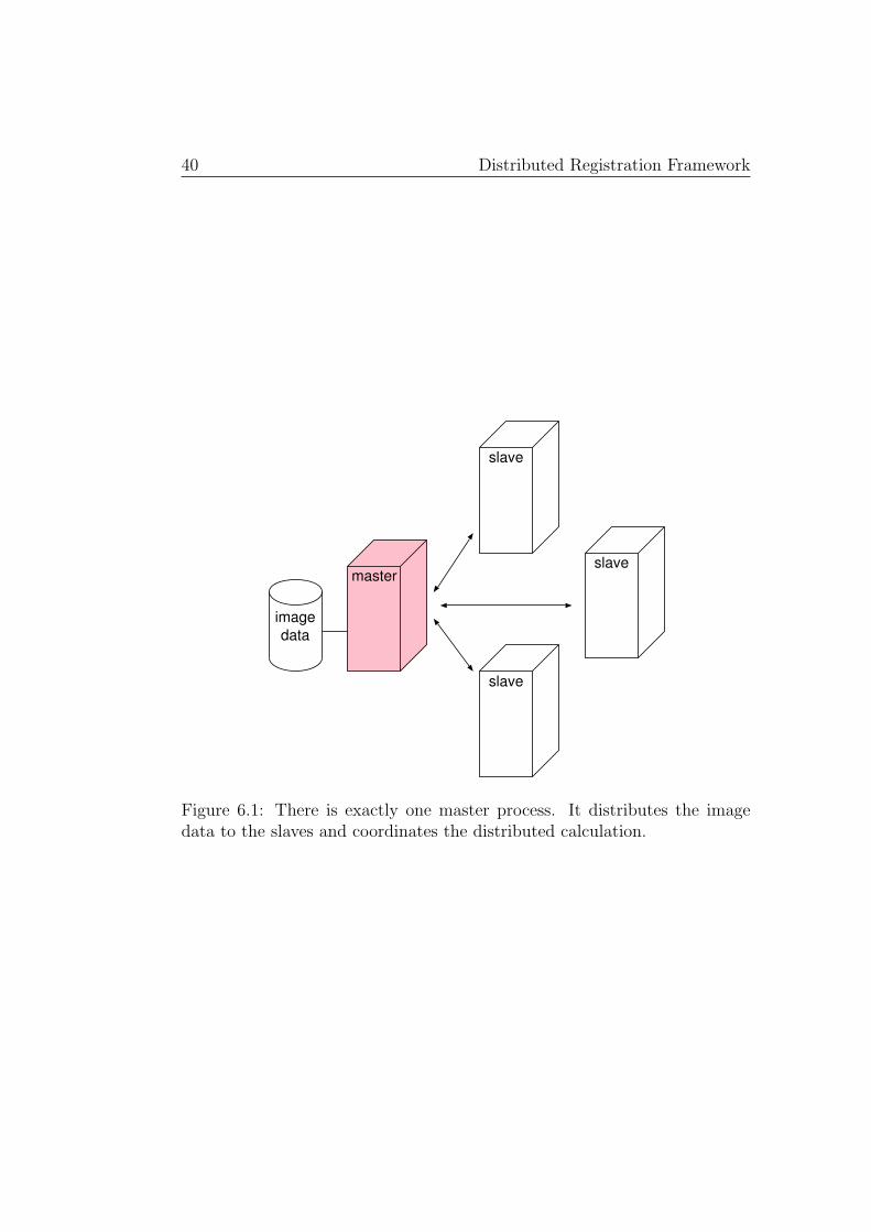
The distributed registration framework extends the existing registrationframework by adding support for parallel metric calculation in a distributedmemory environment. The distributed metric calculation is organized ina master-slave manner as illustrated in Figure 6.1. The master process islocated on the same node as the image data. It is responsible for data dis-tribution as well as for the communication between the existing registrationframework and the slave nodes and it hides the distribution details from theuser. The slaves do the major part of the metric function evaluation andwork in parallel which leads to the targeted speedup. To each slave a regionof the fixed image is assigned. For this part, the respective slave calculatessome intermediate metric value. In intensity based metric functions, such anintermediate value is calculated based on the comparison of each pixel of theassigned fixed image region with the respective pixel of the moving image.The master provides the slaves with the data they need to carry out theircalculations. It further coordinates all steps required to collect and processthe partial results and passes the final result to the registration framework.
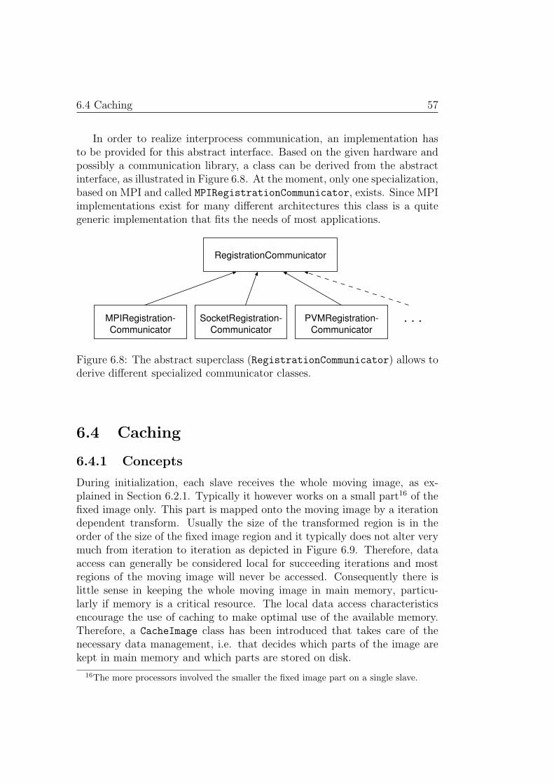
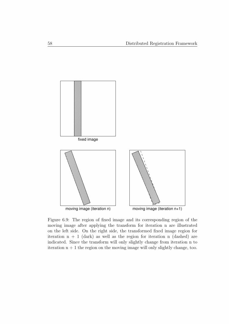
Besides the assigned fixed image region, each slave is provided with thewhole moving image to make sure it has all necessary data at its disposal inorder to calculate the intermediate metric value. Typically, only a small partof this image is accessed, however. Therefore a caching mechanism that canoptionally be enabled has been introduced. This caching mechanism togetherwith the subdivision of the fixed image makes sure that even for large datasize problems memory consumption in the slaves is kept low.
40 Distributed Registration Framework
imagedata
master
slave
slave
slave
Figure 6.1: There is exactly one master process. It distributes the imagedata to the slaves and coordinates the distributed calculation.
6.2 Distributed Metric 41
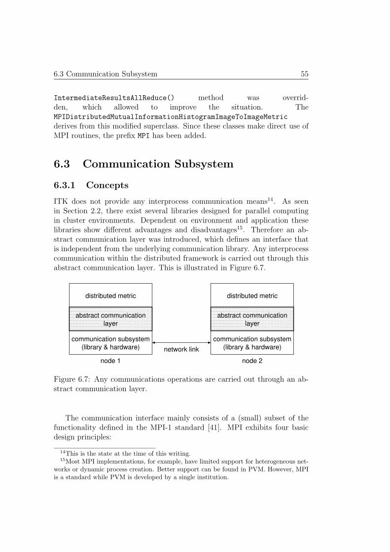
Within the whole distributed framework, an abstract interface is used forall communication tasks. This ensures maximum flexibility with respect tothe underlying hardware and communication subsystem.
These concepts are implemented using the following basic classes:
• DistributedImageToImageMetric
• RegistrationCommunicator
• CacheImage
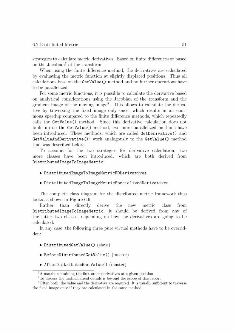
The core element of the distributed registration framework is theDistributedImageToImageMetric class, which is divided into a master anda slave part. It is derived from the itk::ImageToImageMetric class whichserves as a superclass to all similarity functions used within the basic regis-tration framework of ITK.
The DistributedImageToImageMetric class is an abstract superclass. Inorder to create a specialized similarity function, some virtual methods haveto be implemented by derived classes. These functions define the way theactual similarity measure is calculated and therefore determine the actualbehavior of the metric.
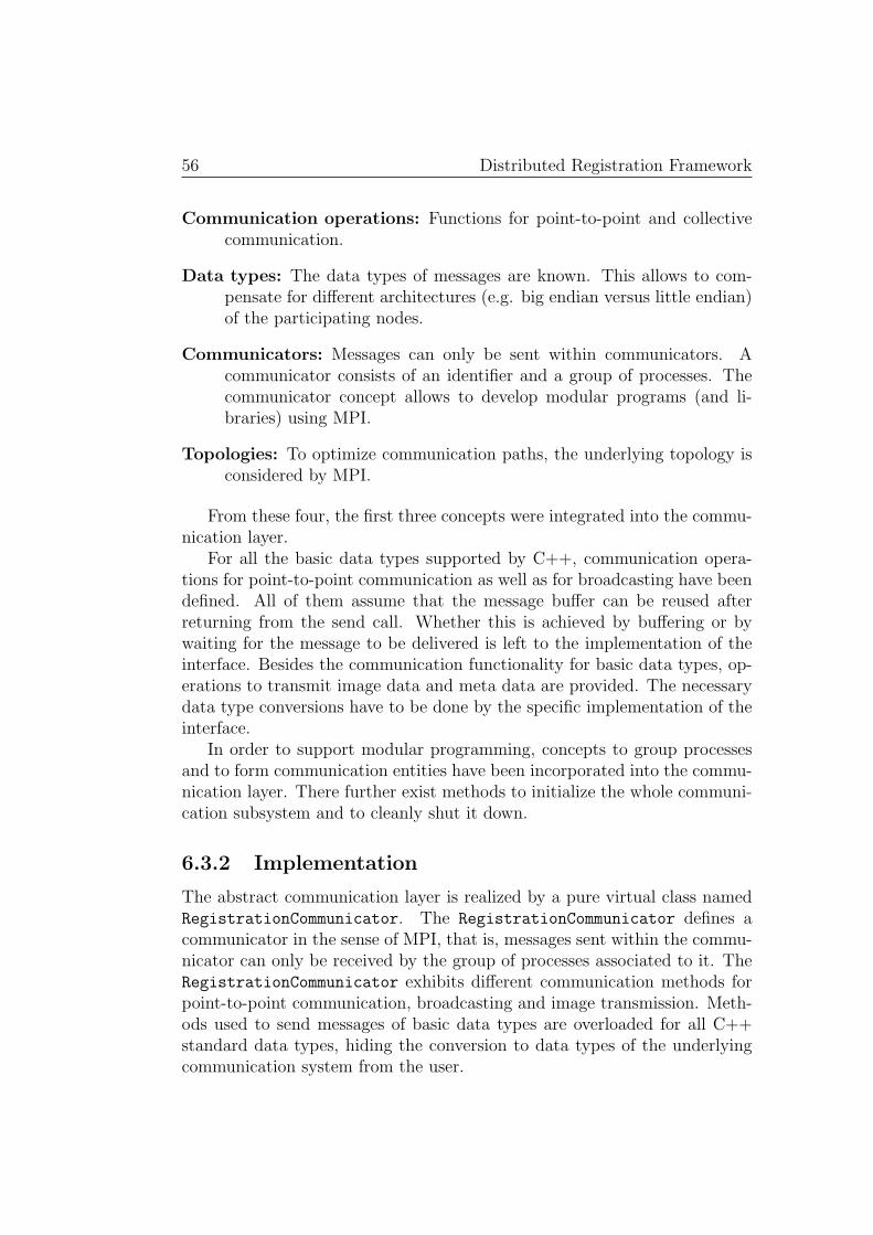
Communication is realized through an abstract class calledRegistrationCommunicator, which provides an interface for all thenecessary communication tasks. Specialized implementations of this inter-face allow to adapt the registration framework to different parallel hardwareand communication libraries. At the moment, only one specialization basedon MPI is realized.
A CacheImage organizes its data in a block structure and makes surethat only recently accessed blocks are kept in main memory, while others arestored on disk. A user can choose whether images are stored as cache- or asusual images, which perform better as long as memory is not critical.
6.2 Distributed Metric
6.2.1 Concepts
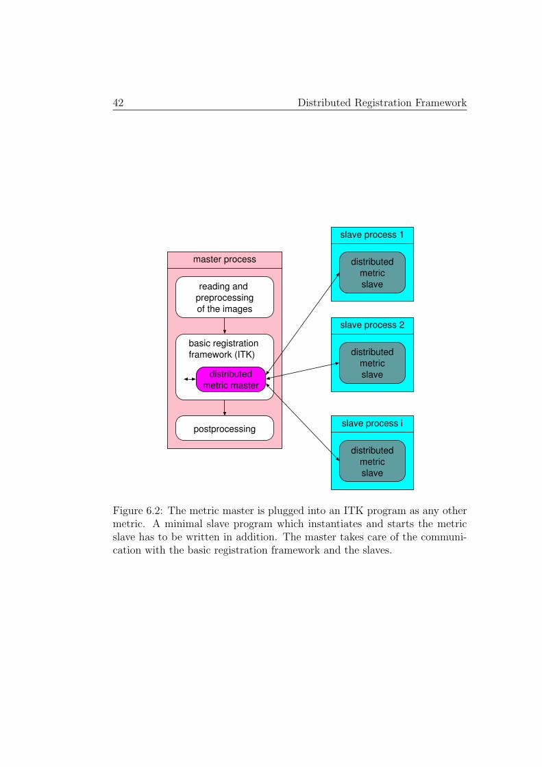
The DistributedImageToImageMetric is the core of the distributed regis-tration framework. It is a closed module which can be plugged into the basicregistration framework, and which consists of a master and a slave part. Themaster part coordinates the whole calculation and thereby hides the distri-bution details from the user while the slaves do the actual work. This basicsetup is illustrated in Figure 6.2.
42 Distributed Registration Framework
master process
reading and preprocessingof the images
basic registrationframework (ITK)
distributedmetric master
postprocessing
slave process 1
distributedmetricslave
slave process 2
distributedmetricslave
slave process i
distributedmetricslave
Figure 6.2: The metric master is plugged into an ITK program as any othermetric. A minimal slave program which instantiates and starts the metricslave has to be written in addition. The master takes care of the communi-cation with the basic registration framework and the slaves.
6.2 Distributed Metric 43
The whole registration process consists of two major stages: Initializationand optimization. They are treated separately in the following sections.
Initialization
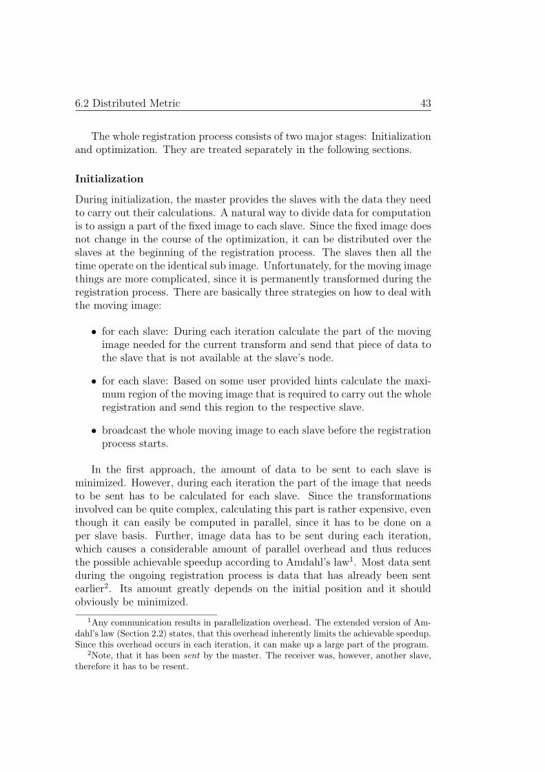
During initialization, the master provides the slaves with the data they needto carry out their calculations. A natural way to divide data for computationis to assign a part of the fixed image to each slave. Since the fixed image doesnot change in the course of the optimization, it can be distributed over theslaves at the beginning of the registration process. The slaves then all thetime operate on the identical sub image. Unfortunately, for the moving imagethings are more complicated, since it is permanently transformed during theregistration process. There are basically three strategies on how to deal withthe moving image:
• for each slave: During each iteration calculate the part of the movingimage needed for the current transform and send that piece of data tothe slave that is not available at the slave’s node.
• for each slave: Based on some user provided hints calculate the maxi-mum region of the moving image that is required to carry out the wholeregistration and send this region to the respective slave.
• broadcast the whole moving image to each slave before the registrationprocess starts.
In the first approach, the amount of data to be sent to each slave isminimized. However, during each iteration the part of the image that needsto be sent has to be calculated for each slave. Since the transformationsinvolved can be quite complex, calculating this part is rather expensive, eventhough it can easily be computed in parallel, since it has to be done on aper slave basis. Further, image data has to be sent during each iteration,which causes a considerable amount of parallel overhead and thus reducesthe possible achievable speedup according to Amdahl’s law1. Most data sentduring the ongoing registration process is data that has already been sentearlier2. Its amount greatly depends on the initial position and it shouldobviously be minimized.
1Any communication results in parallelization overhead. The extended version of Am-dahl’s law (Section 2.2) states, that this overhead inherently limits the achievable speedup.Since this overhead occurs in each iteration, it can make up a large part of the program.
2Note, that it has been sent by the master. The receiver was, however, another slave,therefore it has to be resent.
44 Distributed Registration Framework
It would of course be desirable to know the total region required by eachslave in advance. Then this region could be sent at the beginning of theregistration process and no further calculation and communication overheadoccurs. However, it is a highly non-trivial task to calculate this region inadvance. Only sophisticated user input would allow to do that. The resultinginterface most likely became very complicated and hence difficult to handleand prone to mistakes.
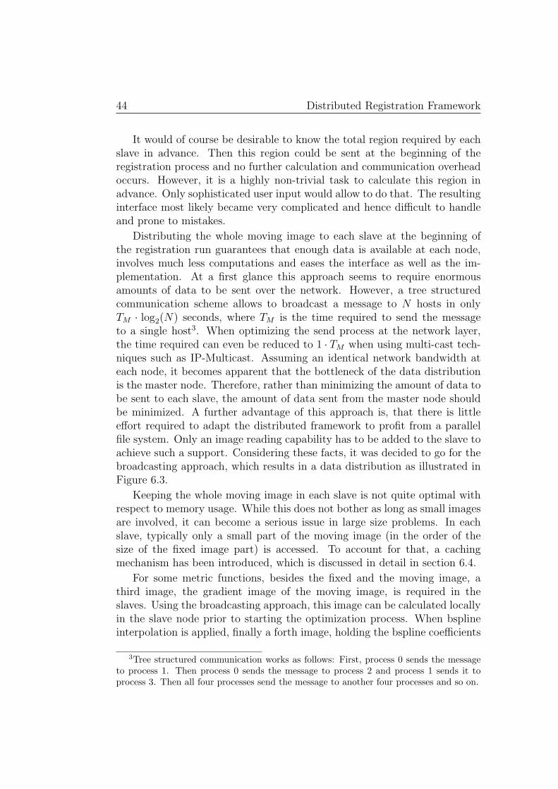
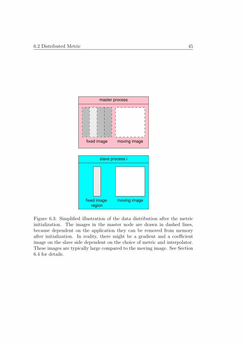
Distributing the whole moving image to each slave at the beginning ofthe registration run guarantees that enough data is available at each node,involves much less computations and eases the interface as well as the im-plementation. At a first glance this approach seems to require enormousamounts of data to be sent over the network. However, a tree structuredcommunication scheme allows to broadcast a message to N hosts in onlyTM · log2(N) seconds, where TM is the time required to send the messageto a single host3. When optimizing the send process at the network layer,the time required can even be reduced to 1 · TM when using multi-cast tech-niques such as IP-Multicast. Assuming an identical network bandwidth ateach node, it becomes apparent that the bottleneck of the data distributionis the master node. Therefore, rather than minimizing the amount of data tobe sent to each slave, the amount of data sent from the master node shouldbe minimized. A further advantage of this approach is, that there is littleeffort required to adapt the distributed framework to profit from a parallelfile system. Only an image reading capability has to be added to the slave toachieve such a support. Considering these facts, it was decided to go for thebroadcasting approach, which results in a data distribution as illustrated inFigure 6.3.
Keeping the whole moving image in each slave is not quite optimal withrespect to memory usage. While this does not bother as long as small imagesare involved, it can become a serious issue in large size problems. In eachslave, typically only a small part of the moving image (in the order of thesize of the fixed image part) is accessed. To account for that, a cachingmechanism has been introduced, which is discussed in detail in section 6.4.
For some metric functions, besides the fixed and the moving image, athird image, the gradient image of the moving image, is required in theslaves. Using the broadcasting approach, this image can be calculated locallyin the slave node prior to starting the optimization process. When bsplineinterpolation is applied, finally a forth image, holding the bspline coefficients
3Tree structured communication works as follows: First, process 0 sends the messageto process 1. Then process 0 sends the message to process 2 and process 1 sends it toprocess 3. Then all four processes send the message to another four processes and so on.
6.2 Distributed Metric 45
master process
fixed image moving image
slave process i
fixed image region
moving image
Figure 6.3: Simplified illustration of the data distribution after the metricinitialization. The images in the master node are drawn in dashed lines,because dependent on the application they can be removed from memoryafter initialization. In reality, there might be a gradient and a coefficientimage on the slave side dependent on the choice of metric and interpolator.These images are typically large compared to the moving image. See Section6.4 for details.
46 Distributed Registration Framework
needs to be kept in the slaves. Typically, the gradient as well as the coefficientimage are large compared to the moving and the fixed image. Since the accesscharacteristics are equal to those for the moving image, the same cachingmechanism can be applied in order to cut down memory usage.
Optimization phase
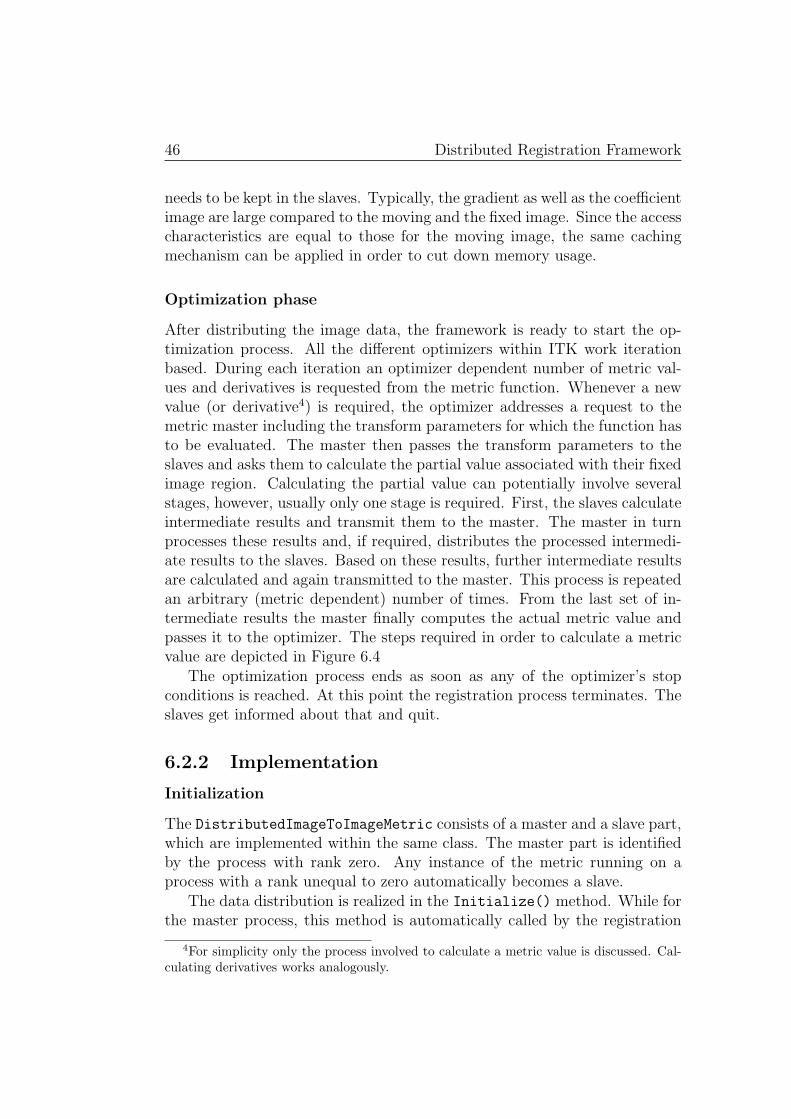
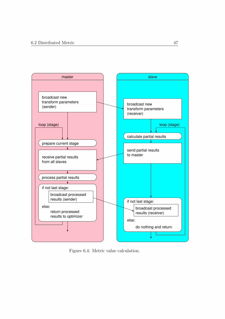
After distributing the image data, the framework is ready to start the op-timization process. All the different optimizers within ITK work iterationbased. During each iteration an optimizer dependent number of metric val-ues and derivatives is requested from the metric function. Whenever a newvalue (or derivative4) is required, the optimizer addresses a request to themetric master including the transform parameters for which the function hasto be evaluated. The master then passes the transform parameters to theslaves and asks them to calculate the partial value associated with their fixedimage region. Calculating the partial value can potentially involve severalstages, however, usually only one stage is required. First, the slaves calculateintermediate results and transmit them to the master. The master in turnprocesses these results and, if required, distributes the processed intermedi-ate results to the slaves. Based on these results, further intermediate resultsare calculated and again transmitted to the master. This process is repeatedan arbitrary (metric dependent) number of times. From the last set of in-termediate results the master finally computes the actual metric value andpasses it to the optimizer. The steps required in order to calculate a metricvalue are depicted in Figure 6.4
The optimization process ends as soon as any of the optimizer’s stopconditions is reached. At this point the registration process terminates. Theslaves get informed about that and quit.
6.2.2 Implementation
Initialization
The DistributedImageToImageMetric consists of a master and a slave part,which are implemented within the same class. The master part is identifiedby the process with rank zero. Any instance of the metric running on aprocess with a rank unequal to zero automatically becomes a slave.
The data distribution is realized in the Initialize() method. While forthe master process, this method is automatically called by the registration
4For simplicity only the process involved to calculate a metric value is discussed. Cal-culating derivatives works analogously.
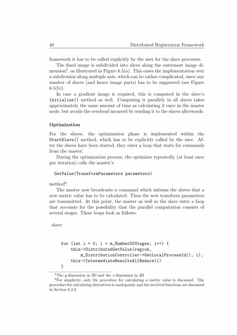
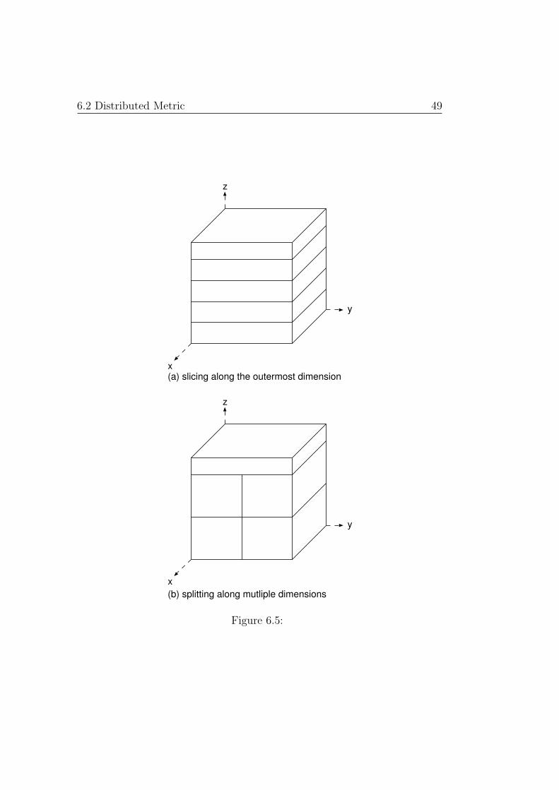
framework it has to be called explicitly by the user for the slave processes.The fixed image is subdivided into slices along the outermost image di-
mension5, as illustrated in Figure 6.5(a). This eases the implementation overa subdivision along multiple axis, which can be rather complicated, since anynumber of slaves (and hence image parts) has to be supported (see Figure6.5(b)).
In case a gradient image is required, this is computed in the slave’sInitialize() method as well. Computing it parallely in all slaves takesapproximately the same amount of time as calculating it once in the masternode, but avoids the overhead incurred by sending it to the slaves afterwards.
Optimization
For the slaves, the optimization phase is implemented within theStartSlave() method, which has to be explicitly called by the user. Af-ter the slaves have been started, they enter a loop that waits for commandsfrom the master.
During the optimization process, the optimizer repeatedly (at least onceper iteration) calls the master’s
GetValue(TransformParameters parameters)
method6.The master now broadcasts a command which informs the slaves that a
new metric value has to be calculated. Then the new transform parametersare transmitted. At this point, the master as well as the slave enter a loopthat accounts for the possibility that the parallel computation consists ofseveral stages. These loops look as follows:
The slaves first calculate the intermediate results for the current stage byinvoking their DistributedGetValue() method and then send them to themaster. To ease the send process, all intermediate results are transmitted asan array of type double. The master first receives the intermediate resultsfrom all the slaves, then processes them and finally redistributes the processedresults to the slaves, if the current stage is not yet the last one.
The IntermediateResultsAllReduce() method was introduced, be-cause in some cases this operation can be performed more efficiently thanshown here. If a more efficient solution exists, a derived metric class canrealize it by overriding IntermediateResultsAllReduce().
After exiting the loops, the final metric value is stored on the metricmaster. The master’s GetValue() function now returns this value to theregistration framework. The slave, on the other hand, waits for a new com-mand to be processed.
Above steps are repeated for each iteration during the optimization pro-cess. Eventually, the optimizer reaches one of its stop conditions and theoptimization process - and the registration run - terminates. At that time,the slaves are waiting for another command to be processed. Therefore, anexit command is sent to all the slaves which now terminate.
6.2.3 Creating new Metric Functions
The basic idea to create a new metric function is to derive a specializedclass from the DistributedImageToImageMetric. However, there are two
6.2 Distributed Metric 51
strategies to calculate metric derivatives: Based on finite differences or basedon the Jacobian7 of the transform.
When using the finite difference method, the derivatives are calculatedby evaluating the metric function at slightly displaced positions. Thus allcalculations base on the GetValue() method and no further operations haveto be parallelized.
For some metric functions, it is possible to calculate the derivative basedon analytical considerations using the Jacobian of the transform and thegradient image of the moving image8. This allows to calculate the deriva-tive by traversing the fixed image only once, which results in an enor-mous speedup compared to the finite difference methods, which repeatedlycalls the GetValue() method. Since this derivative calculation does notbuild up on the GetValue() method, two more parallelized methods havebeen introduced. These methods, which are called GetDerivative() andGetValueAndDerivative()9 work analogously to the GetValue() methodthat was described before.
To account for the two strategies for derivative calculation, twomore classes have been introduced, which are both derived fromDistributedImageToImageMetric:
The complete class diagram for the distributed metric framework thuslooks as shown in Figure 6.6.
Rather than directly derive the new metric class fromDistributedImageToImageMetric, it should be derived from any ofthe latter two classes, depending on how the derivatives are going to becalculated.
In any case, the following three pure virtual methods have to be overrid-den:
• DistributedGetValue() (slave)
• BeforeDistributedGetValue() (master)
• AfterDistributedGetValue() (master)
7A matrix containing the first order derivatives at a given position8To discuss the mathematical details is beyond the scope of this report9Often both, the value and the derivative are required. It is usually sufficient to traverse
the fixed image once if they are calculated in the same method.
52 Distributed Registration Framework
itk::ImageToImageMetric
- abstract GetValue()- abstract GetDerivative()- GetValueAndDerivative() (using GetValue() and GetDerivative())
DistributedImageToImageMetric
- GetValue() (using DistributedGetValue())
- abstract DistributedGetValue()- abstract BeforeDistributedGetValue()- abstract AfterDistributedGetValue()- communication functions
DistributedImageToImageMetric-FDDerivatives
- GetDerivative() (using finite differences and GetValue())
- functions to control finite difference parameters
- abstract DistributedGetDerivative()- abstract BeforeDistributedGetDerivative()- abstract AfterDistributedGetDerivative()- abstract DistributedGetValueAndDerivative()- BeforeDistributedGetValueAndDerivative() (using BeforeDistributedGetValue and BeforeDistributedGetDerivative)- AfterDistributedGetValueAndDerivative() (using AfterDistributedGetValue and AfterDistributedGetDerivative)
Figure 6.6: Class diagram for the distributed metric mod-ules. New metric functions should either be derivedfrom DistributedImageToImageMetricFDDerivatives (forderivative calculation based on finite differences) or fromDistributedImageToImageMetricSpecializedDerivatives (for derivativecalculation by a user defined method).
6.2 Distributed Metric 53
The core method is the DistributedGetValue() method, which calcu-lates the partial results for each stage10.
The partial results have to be stored in the class memberm IntermediateResults, which is an array of type double. The first ar-ray index is used by the master to identify the process. For the slaves, andtherefore within the DistributedGetValue() method, this index is alwayszero. The second array index denotes the stage and the third index is usedto identify the n-th value of the intermediate result for the current stage11.The number of pixels considered during the calculation of the partial resulthave to be stored in the m NumberOfPixels member variable.
The method BeforeDistributedGetValue() allows to perform somesteps that prepare the master to receiving the partial results. Often, nospecial steps have to be carried out. In this case, the method can just consistof an empty implementation.
The method AfterDistributedGetValue() finally processes the partialresults provided by the slaves. In the final stage, the result of the processingstep has to be stored in the m Measure member variable. It is the value storedin this variable, which is returned to the registration framework as the valueof the metric function.
For many metric functions these are all the steps that have to be doneto make them available to the distributed framework. However, thereare some further cases that have to be considered. If a metric is derivedfrom the DistributedImageToImageMetricSpecializedDerivatives
class, it has further to implement the DistributedGetDerivative(),the BeforeDistributedGetDerivative(), theAfterDistributedGetDerivative(), and optionally theDistributedGetValueAndDerivative() method.
As mentioned earlier, the IntermediateResultsAllReduce() methodcan be overridden in order to profit from a more efficient method to pro-cess and redistribute the intermediate results.
Further, in some cases the predefined format for storage of intermediateresults might not be suited. In order to properly treat a custom formatfor intermediate results, the following communication methods have to beoverridden:
• SendIntermediateResultsToMaster()
• ReceiveIntermediateResultsFromSlaves()
10usually only one stage is involved, however sometimes it might make sense to calculatethe metric value in a multiple stage process
11An intermediate result can consist of several values, that are transmitted as arrays.The third index points to the n-th value inside this array
54 Distributed Registration Framework
• SendProcessedIntermediateResultsToSlaves()
• ReceiveProcessedIntermediateResultsFromMaster()
6.2.4 Implemented Metric Functions
Based on above guidelines, the following metric functions have been imple-mented:
The first two metric functions both implement a mean squares12 measure.While the first metric calculates derivatives based on finite differences, thesecond one uses a more efficient method based on a gradient image and theJacobian of the transform.
The third metric serves as an abstract superclass for metric func-tions that operate on the joint histogram of the two images. TheDistributedMeanSquaresHistogramImageToImageMetric as well as theMutualInformationHistogramImageToImageMetric directly build uponthis superclass. As indicated by their names, they define a mean squaresmeasure and a measure based on mutual information, respectively13. Themutual information metric is applicable in inter- as well as intra-model ap-plications.
The histogram based metric functions incur a large com-munication overhead, as will be shown in Section 7.5.3.In the MPIDistributedHistogramImageToImageMetric, the
12Squared error or the pixel intensities divided by the number of pixels considered inorder to normalize the value.
13There are two reasons that legitimate the existence of this third mean squares met-ric: First, it often requires a lower number of multiplications than the other approaches.Second, since in a histogram several intensity values can be subsumed into one bin, theresult is not necessarily the same as for the other approaches.
6.3 Communication Subsystem 55
IntermediateResultsAllReduce() method was overrid-den, which allowed to improve the situation. TheMPIDistributedMutualInformationHistogramImageToImageMetric
derives from this modified superclass. Since these classes make direct use ofMPI routines, the prefix MPI has been added.
6.3 Communication Subsystem
6.3.1 Concepts
ITK does not provide any interprocess communication means14. As seenin Section 2.2, there exist several libraries designed for parallel computingin cluster environments. Dependent on environment and application theselibraries show different advantages and disadvantages15. Therefore an ab-stract communication layer was introduced, which defines an interface thatis independent from the underlying communication library. Any interprocesscommunication within the distributed framework is carried out through thisabstract communication layer. This is illustrated in Figure 6.7.
abstract communicationlayer
communication subsystem(library & hardware)
distributed metric
abstract communicationlayer
communication subsystem(library & hardware)
distributed metric
network link
node 1 node 2
Figure 6.7: Any communications operations are carried out through an ab-stract communication layer.
The communication interface mainly consists of a (small) subset of thefunctionality defined in the MPI-1 standard [41]. MPI exhibits four basicdesign principles:
14This is the state at the time of this writing.15Most MPI implementations, for example, have limited support for heterogeneous net-
works or dynamic process creation. Better support can be found in PVM. However, MPIis a standard while PVM is developed by a single institution.
56 Distributed Registration Framework
Communication operations: Functions for point-to-point and collectivecommunication.
Data types: The data types of messages are known. This allows to com-pensate for different architectures (e.g. big endian versus little endian)of the participating nodes.
Communicators: Messages can only be sent within communicators. Acommunicator consists of an identifier and a group of processes. Thecommunicator concept allows to develop modular programs (and li-braries) using MPI.
Topologies: To optimize communication paths, the underlying topology isconsidered by MPI.
From these four, the first three concepts were integrated into the commu-nication layer.
For all the basic data types supported by C++, communication opera-tions for point-to-point communication as well as for broadcasting have beendefined. All of them assume that the message buffer can be reused afterreturning from the send call. Whether this is achieved by buffering or bywaiting for the message to be delivered is left to the implementation of theinterface. Besides the communication functionality for basic data types, op-erations to transmit image data and meta data are provided. The necessarydata type conversions have to be done by the specific implementation of theinterface.
In order to support modular programming, concepts to group processesand to form communication entities have been incorporated into the commu-nication layer. There further exist methods to initialize the whole communi-cation subsystem and to cleanly shut it down.
6.3.2 Implementation
The abstract communication layer is realized by a pure virtual class namedRegistrationCommunicator. The RegistrationCommunicator defines acommunicator in the sense of MPI, that is, messages sent within the commu-nicator can only be received by the group of processes associated to it. TheRegistrationCommunicator exhibits different communication methods forpoint-to-point communication, broadcasting and image transmission. Meth-ods used to send messages of basic data types are overloaded for all C++standard data types, hiding the conversion to data types of the underlyingcommunication system from the user.
6.4 Caching 57
In order to realize interprocess communication, an implementation hasto be provided for this abstract interface. Based on the given hardware andpossibly a communication library, a class can be derived from the abstractinterface, as illustrated in Figure 6.8. At the moment, only one specialization,based on MPI and called MPIRegistrationCommunicator, exists. Since MPIimplementations exist for many different architectures this class is a quitegeneric implementation that fits the needs of most applications.
RegistrationCommunicator
SocketRegistration-Communicator
MPIRegistration-Communicator
PVMRegistration-Communicator
. . .
Figure 6.8: The abstract superclass (RegistrationCommunicator) allows toderive different specialized communicator classes.
6.4 Caching
6.4.1 Concepts
During initialization, each slave receives the whole moving image, as ex-plained in Section 6.2.1. Typically it however works on a small part16 of thefixed image only. This part is mapped onto the moving image by a iterationdependent transform. Usually the size of the transformed region is in theorder of the size of the fixed image region and it typically does not alter verymuch from iteration to iteration as depicted in Figure 6.9. Therefore, dataaccess can generally be considered local for succeeding iterations and mostregions of the moving image will never be accessed. Consequently there islittle sense in keeping the whole moving image in main memory, particu-larly if memory is a critical resource. The local data access characteristicsencourage the use of caching to make optimal use of the available memory.Therefore, a CacheImage class has been introduced that takes care of thenecessary data management, i.e. that decides which parts of the image arekept in main memory and which parts are stored on disk.
16The more processors involved the smaller the fixed image part on a single slave.
Figure 6.9: The region of fixed image and its corresponding region of themoving image after applying the transform for iteration n are illustratedon the left side. On the right side, the transformed fixed image region foriteration n + 1 (dark) as well as the region for iteration n (dashed) areindicated. Since the transform will only slightly change from iteration n toiteration n + 1 the region on the moving image will only slightly change, too.
6.4 Caching 59
In order to efficiently move data portions from main memory to disk andvice versa, data is preferably stored in a block structure rather than line byline as this is done in ITK. This is depicted in Figure 6.10. Therefore, theCacheImage organizes its data in blocks. Whenever a pixel is accessed, itis checked whether the corresponding block resides in main memory. If not,the new block is loaded from disk and the block that has not been accessedfor the longest time is released from main memory.
To avoid occupying large amounts of swap space that could be used byother processes, data on disk is stored in a regular file. Memory mappedaccess is used in order to perform read and write operations on the file.
In case of the moving image, the CacheImage is integrated into aCacheInterpolator. Three of them exist, in accordance with the threeinterpolator types (nearest neighbor, linear and bspline) present in ITK. Incase of the gradient image, the cache image is directly located in the metricslaves.
The gradient image is large compared to the moving image, because apixel consists of a floating point value for each derivative. Typically it con-sumes between 8 and 24 times as much memory as the moving image17.Caching this image reduces the memory consumption during the ongoingoptimization process. However, the memory peak resulting during the cre-ation of the gradient image can already cause serious problems. A systemmight run out of physical memory which causes swapping and slows downthe creation process. What makes things worse is the fact that there are op-erating systems18, that do not allow a process to return freed memory to theoperating system. Therefore, the process size will not drop even during opti-mization, where due to caching only small amounts of memory are used. Theunused memory (which is most likely swapped out) reduces the swap spaceavailable to other processes. Because of these problems, the memory peakoccurring during gradient image generation should be avoided. The stream-ing concept of ITK allows to create images in pieces. Creating the gradientimage block by block and directly writing these blocks to disk avoids theundesirable memory peak.
In memory uncritical problems, the framework performs better withoutcaching. Therefore, it is by default disabled. In order to enable caching, acached interpolator has to be provided in case of the moving image, and aflag has to be set in case of the gradient image.
17A pixel of the moving image is typically represented by one or two bytes and a deriva-tive typically by a double value which takes 8 bytes. In 2D there are 2 derivatives yielding16 bytes, and in 3D there are 3 derivatives yielding 24 bytes per pixel.
Figure 6.10: Top: Linear data structure as it is used by the standard ITKimage. Pixels are stored line by line in a single huge array, as indicatedby the increasing numbers. When data for the shadowed region should bekept in memory, and it should be possible to move blocks of 16 pixels toand from disk, the area marked with bold lines is affected. Bottom: Thesame is illustrated for an image that stores data in blocks of 4 by 4 pixels.In the first case, 16 × 16 = 256 pixels are affected, in the second case only8× 16 = 128 pixels. In reality, both, image as well as block size is typicallymuch larger than in this illustration.
6.4 Caching 61
6.4.2 Implementation
Pixels that do not belong to the fixed image are accessed after apply-ing a transform. Therefore, any pixel values are retrieved by the image’sGetPixel() method and no iterators are used. This fact considerable easesthe implementation of an image that stores data in blocks, since no compli-cated iterators that need to traverse these blocks have to be implemented.Rather, any index calculation can be carried out within the GetPixel()
method. Index calculations turn out to be more complex than for usualimage data structures, despite the use of index tables to speed them up.Consequently pixel access performs worse when CacheImages are used.
The block handling is also realized in the GetPixel() method. Thewhole data is written into an ordinary file, block by block. Memory mappedfile access allows to efficiently move blocks to and remove them from mainmemory. A FileMapper class wraps the mapping process in order to hide thedifferences of memory mapped file access in Windows and Unix. Whenevera pixel is accessed and the corresponding block does not reside in memory,the respective region of the file is mapped to a new view. The view of theblock that has not been accessed for the longest time is unmapped.
Caching of the moving image is realized by new interpolator classes,namely
• NearestNeighborCacheInterpolateImageFunction
• LinearCacheInterpolateImageFunction
• BSplineCacheInterpolateImageFunction
Two main reasons led to the decision that the cache image should becreated within the interpolator and not within the metric class. A firstreason is, that the bspline interpolator works on a coefficient image, ratherthan directly on the moving image. This coefficient image is the one that hasto be cached, and it has to be created inside of the interpolator. Creating thecached image inside the nearest neighbor and the linear interpolator allowsto treat all the cases almost identically. A second reason that speaks in favorof wrapping the cache image inside the interpolator are several type conflictsthat would have had to be resolved when storing the image in the metric.
Caching of the gradient image is realized inside the metric class. In orderto avoid the undesired memory peak, the gradient image is created blockby block and these blocks are directly written disk. Since the gradient filterapplied in ITK image metrics does not support streaming it was replaced bya combination of a smoothing filter (itk::DiscreteGaussianImageFilter)
62 Distributed Registration Framework
and a simpler gradient filter (itk::GradientImageFilter) that is streamingcapable.
Chapter 7
Evaluation
When evaluating a parallel realization of an algorithm, several measures areof interest. The measures used to assess the methods developed through-out this project are briefly introduced within the following section. Then asoftware library (MPE) that allows the examination of performance param-eters within a parallel program is presented followed by the discussion of themethodology, the scenarios used for, and the results of the evaluation of thedistributed registration framework.
7.1 Measures
Usually, people are interested in the reduction of computing time in the firstplace. Recall from Section 2.2, that reduction in computing time is definedas parallel speedup
SN = TS/TN (7.1)
and that another, closely related measure called parallel efficiency
EN = SN/N (7.2)
has been introduced. In these formulas, N denotes the number of proces-sors, TN the execution time of the parallel program on N processors, and TS
the execution time of the best sequential algorithm on one processor. Notethat it is generally difficult to define TS, because of several reasons. Whichalgorithm performs best can depend on several factors, the best algorithmcan change over time (since new, better algorithms are developed) and it isnot clear on which hardware the time is measured. Therefore, in practice TS
64 Evaluation
usually denotes the execution time of a good sequential algorithm1.
The parallel efficiency usually depends on the number of processors as wellas on the problem size W (using the definition of [42](p. 129), W becomesbasically equal to TS
2). Due to non parallelizable code and an increasingcommunication as well as synchronization overhead, the parallel efficiencydecreases with an increasing number of processors. On the other hand, anincreasing problem size often increases efficiency, since the calculation timeincreases relative to the overhead. A system that allows to keep the efficiencyat a fixed value for an increasing number of processors, if the problem sizeis adjusted accordingly, is called scalable. The function that defines how Whas to be increased with respect to N in order to keep the efficiency fixed iscalled isoefficiency function. To look at this phenomena more closely, let usdefine the total overhead
To = N · TN −W , (7.3)
which subsumes any work that is not incurred by the fastest known se-quential algorithm. As seen before, the total overhead is a function of theproblem size as well as the number of processors: To(N, W ). Using equation7.3, the parallel execution time can be written as a function of the problemsize, the number of processes and the total overhead function:
TN =W + To(W, N)
N
Substituting TN in equations 7.1 and 7.2 results in the following expres-sion for the parallel efficiency:
EN =1
1 + To(N, W )/W(7.4)
From equation 7.4 it becomes apparent, that the efficiency does notchange if To(N, W )/W is constant. Replacing EN in 7.4 with the desiredvalue E for the efficiency and reformulating the equation yields:
W =E
1− ETo(N, W ) (7.5)
1For the evaluation of the parallel registration framework, TS was the time used by anequivalent program composed of standard ITK modules.
2The authors of [42] state, that problem size should be proportional to the total numberof basic computational steps involved, which is proportional to TS . If the unit to measureW is normalized accordingly, W thus becomes equal to TS . This is arguable when factorslike disk swapping slow down the computation.
7.2 The Multi Processing Environment (MPE) Library 65
This is an implicit representation of the isoefficiency function. Oftenequation 7.5 can be reformulated such that W is expressed as a function ofN , which results in an explicit representation of the isoefficiency function.
The isoefficiency function defines the ease with which the efficiency ofa parallel system can be kept fixed by increasing the problem size. It cantherefore be considered as a measure for scalability . A “small” isoefficiencyfunction denotes that a little increase of the problem size is sufficient inorder to maintain the efficiency for an increasing number of processors, whichmeans that the algorithm scales well.
With a growing problem size, memory requirements usually increase.Therefore, memory requirements have to be considered carefully when ana-lyzing scalability. Often it is assumed that the amount of available memorygrows equally to the number of processors (this is quite reasonable for clustercomputing). It is then possible to change above definition of a scalable systemby adding a memory constraint: A system is scalable if the efficiency can bekept fixed for a growing number of processes by increasing the problem sizesuch that the memory requirement per processor is constant (or decreasing).
7.2 The Multi Processing Environment
(MPE) Library
The Multi Processing Environment (MPE) library [43] provides features forgraphics output, debugging and performance analysis of MPI programs. Itis an open source library developed at the Argonne National Laboratory.Here, only a brief introduction to the functionality for performance analysisis given.
The performance analysis using MPE is based on logging of events usinghighly accurate time stamps. There is an automatic mode that enclosesevery MPI routine with calls to the MPE library which in turn creates anentry in a log file for the beginning and the end of the routine. Further, itis possible to create user defined events by inserting according calls to theMPE library into the code. MPE gathers all the information logged by thedifferent processes, corrects the possible misalignment and drift of clocks andfinally creates a single log file.
Typically a log file generated by MPE is viewed by some graphical toolthat displays all the logged events as time-lines. The most popular viewer isJumpshot , which comes with the MPE distribution. An example of a time-line representation of an MPE log file using Jumpshot is shown in Figure7.1.
66 Evaluation
Figure 7.1: A screenshot of the Jumpshot output of an MPE log file. Therows represent the single processes and the x-direction the elapsed time sinceprocess start. Colored boxes depict states (such as computing time, broadcastoperations, etc.) and arrows indicate point to point communications.
7.3 Methodology 67
Inserting timing statements into a program obviously incurs some over-head. In our case, this overhead is small with respect to computing timesand can safely be neglected during performance analysis. However, whendeveloping an application based on the parallel registration framework thisoverhead is not desired. MPE logging is only in effect if MPE is linked tothe program. Since this decision is made at link time, no overhead occurs ifMPE is not linked. In order to disable custom calls to MPE routines, a com-piler directive has been defined that allows to switch these calls on and off atcompile time and which can be set using CMake3 during the configurationof the parallel registration framework.
7.3 Methodology
The goal of the evaluation was to examine the developed methods with re-spect to speedup, efficiency and scalability. When analyzing the scalability,memory issues were taken into account.
These measures were acquired for three different sample scenarios. A sam-ple scenario consists of a combination of metric function, optimizer, transformand interpolator with their respective parameters.
Speedup and efficiency can be quantified for a fixed problem size by mea-suring the execution times of the parallel program as well as of the “best” se-quential algorithm. The “best” sequential algorithm required to get the timeTS is considered to be the equivalent algorithm implemented using standardITK modules. TS is measured on a single node of the workstation cluster.Execution time is measured as wall-clock time, which is the time (such as thesystem time) elapsed between the process start and its termination. Usingwall-clock time is common practice when evaluating parallel performance.
In order to evaluate the scalability, it is necessary to adjust the problemsize and to closely watch the memory consumption, as explained in Section7.1. Therefore, for each scenario memory usage as well as speedup has to beexamined for an increasing problem size. The increase in problem size canbe quantified by measuring the increase of TS
4. To modify the problem size,obviously the size of the input images can be changed. For larger imagesmore pixels have to be compared and consequently problem size increases.An other option to get a larger problem size is to ask for higher accuracy.This can be achieved by adjusting the optimizer parameters that define the
3A makefile generation tool4This is arguable in cases where the sequential program is slowed down due to disk
swapping.
68 Evaluation
stop conditions. Basically, a higher accuracy asks for a larger number ofiterations and consequently problem size increases.
Obviously it would be interesting to gain a deeper insight into the per-formance parameters than by just measuring the total execution time andmemory consumption. Using the MPIRegistrationCommunicator as thecommunication interface (see Section 6.3 for details) a program based on theparallel registration framework becomes an MPI application which allows touse MPE to gain such an insight. By automatic profiling, MPE allows tomeasure the overhead of the MPI routines (which is mainly communicationoverhead). Customized MPE calls further permit to measure time spent inparticular parts of the code, such as the non parallelizable fraction f , theinitialization phase, work carried out by the optimizer or time spent by theprocesses waiting for each other. Figure 7.2 shows for the case of the opti-mization phase, how the parallel algorithm can be subdivided into differentparts.
During the evaluation, the following values have been analyzed usingMPE:
• time spent in the initialization phase
• time spent to send the moving and the fixed image
• time spent by the optimizer
• time spent to calculate the intermediate values and derivatives
• idle time of the slaves (waiting for new parameters)
Unlike the measures described in Section 7.1, these values do not pro-vide the possibility to compare the parallel framework with other parallelalgorithms. However, they give insight into strengths and deficiencies of theparallel framework and allow to derive conclusions on how to further improveit.
Measurement Conditions
Experiments were carried out on Unix workstations at ETH Zurich (Tardiscluster) as well as on a Windows cluster at Nizhny Novgorod State Univer-sity (NNSU). The Tardis cluster consists of up to 78 identical Sun-Blade-100workstations with 512 MB RAM and about 30 Sun-Blade-1500 workstations.Experiments should only be carried out on the Sun-Blade-100 machines.They are connected by a 100 Mbit Ethernet.
7.3 Methodology 69
command + parameters
prepare partialresults
process partialresults
calculate partialresults
partialresults
GetValue
Value
process value(optimizer)
GetValue
...
master
registrationframework metric
slave
communication overhead
parallel fraction
non parallel fraction (metric)
non parallel fraction (optimizer)
Figure 7.2:
70 Evaluation
The Windows cluster at NNSU consists of 2 servers with 4 Pentium-III700 MHz CPUs each, 12 servers with 2 Pentium-III 1 GHz CPUs each, and 12workstations with a single Pentium-IV 1.3 GHz CPU. The different machineshave 512, 256 and 128 MB of RAM, respectively. The server machines areconnected with a 1000 Mbit, and the workstations with a 100 Mbit Ethernetnetwork.
Any experiments for speedup and efficiency were carried out at least threetimes. The workstations at ETH were not guaranteed to be free of interfer-ence originating from other users. Further, any jobs had to be run withlowest priority (nice 19). This caused a significant load imbalance. Since theparallel framework does not provide dynamic load balancing, only the resultwith the lowest interference (i.e. the experiment with the lowest wall-clocktime) was taken.
On the windows cluster at NNSU eight Pentium-III 1 GHz machines (i.e.16 processors) could be reserved to carry out the experiments. Since theywere supposed to be free of interfering load5, averages times were taken forthe results acquired by the experiments on this system.
The master-slave architecture of the parallel registration frameworkcauses one process (the master process) to be idle most of the time. Thisprocess can be run on the same processor as one of the slave processes, asillustrated in Figure 7.3 (a). In this setup, N + 1 processes (1 master and Nslaves) are run on N processors.
Unfortunately, it was cumbersome to automatically run a large numberof experiments like that at the Unix cluster at ETH. Therefore, the N + 1processes were run on N + 1 processors as illustrated in Figure 7.3 (b).Speedup and efficiency values were, however, calculated with respect to N6.Some specially set up experiments proved, that no change in performancecan be observed between the two configurations.
The Windows cluster also caused difficulties to run experiments as shownin Figure 7.3, since each node consists of two CPUs there. The operatingsystem would automatically place the second process on the second CPU.Therefore, only the experiments on 16 processors (with 17 processes) wererun in the configuration as shown in Figure 7.3 (a).
During all the experiments, MPE logging was enabled. The overheadwith respect to timing is supposed to be negligible. However, the memory
5Unfortunately this was not entirely true as will be shown in Section 7.4.2. However,the load was the same for all experiments.
6Parallel speedup and efficiency are defined with respect to the number of processors.Strictly speaking, they would therefore have had to be related to N + 1 when usingconfiguration (b). However the results would have become difficult to interpret and wouldnot have reflected the actual character of the parallelization.
7.3 Methodology 71
. . .master
slave 1
1
slave 2
2
slave N
N
(a) N+1 processes (master + N slaves) on N processors
. . .
master
1
slave 1
2
slaveN-1
N
slave N
N+1
(b) N+1 processes (master + N slaves) on N+1 processors
Figure 7.3: The parallel framework can be run in two different configurations.In configuration (a), N slaves sit on N processors. Thereby, one processoris shared between a slave an the master. Since the master is idle most ofthe time, performance is not affected. In configuration (b), each process sitson its own CPU. Experiments have been carried out with configuration (b)(except of those on 16 processors at NNSU).
72 Evaluation
measurements might have been influenced by the logging process, since forperformance reasons, log files are kept in main memory until process termi-nation.
7.4 Sample Scenarios
Three sample scenarios addressing different registration tasks have been cre-ated to evaluate the parallel registration framework. These scenarios arebriefly presented in the following sections.
7.4.1 Three Dimensional Rigid Problem
The first scenario addresses a rigid registration problem in 3 dimensions. Thescenario consists of the following components:
Two micro CT images7 of a mouse femur taken from different points ofview serve as the input to the program. The original images have a resolutionof 512 × 512 × 1006 pixels encoded with 2 bytes (65536 gray levels). Thisresults in approximately 500 MB per image. For the experiments, the imageswere downscaled to the following resolutions:
• scale 1: 52× 52× 101 pixels (534 KB)
• scale 2: 65× 65× 127 pixels (1048 KB)
• scale 4: 82× 82× 160 pixels (2102 KB)
• scale 8: 103× 103× 202 pixels (4186 KB)
• scale 16: 130× 130× 254 pixels (8384 KB)
7The images originate from Steven Boyd, PhD, Department of Mechanical and Manu-facturing Engineering, University of Calgary, Canada.
7.4 Sample Scenarios 73
• scale 32: 163× 163× 320 pixels (16606 KB)
• scale 64: 205× 205× 403 pixels (33079 KB)
The most important property of the scenario is the large amount of datawhen using full resolution. The optimizer requires gradients which are cal-culated by the metric by a closed form rather than by finite differences.Therefore, a gradient image has to be calculated in the initialization step.This causes a rather large non-parallelizable fraction of the code8 as well asincreased memory requirements because of the large gradient image.
7.4.2 Two Dimensional Problem based on Bspline De-formable Transform
The second scenario addresses a simple deformable problem in two dimen-sions. It consists of the following components:
The deformation field is defined by a bspline deformable transform. Anexample of such a deformation field is illustrated in Figure 7.4. For thescenario, grid-points on a grid of size 5 × 5 were displaced to well definedpositions. Since third order bsplines were used, the total number of transformparameters was (5 + 3)× (5 + 3) = 64.
Two slices of a brain image (one of which was intentionally deformed)taken from the ITK examples serve as the input to the program. The originalimages have a size of 221× 257 pixels encoded with 1 byte (256 gray-levels).For the experiments, they were upscaled to the following resolutions:
• scale 1: 221× 257 (56 KB)
• scale 2: 313× 364 (112 KB)
8The whole gradient image is calculated on all the slaves, which is basically equivalent tocalculating it once non-parallelized. This step could be parallelized however (see Section 8).
74 Evaluation
Figure 7.4: The bspline deformable transform allows to define a de-formation field by displacing grid-points. The deformation in betweenthe grid points is calculated using bspline interpolation.(image modifiedfrom http://www.cs.rpi.edu/courses/spring04/imagereg/lectureBSplines.ppt(29 September 2004))
• scale 4: 442× 514 (222 KB)
• scale 8: 626× 727 (445 KB)
• scale 16: 884× 1028 (888 KB)
Due to the computationally intensive bspline interpolator, it takes ratherlong to calculate a single metric value (and derivative) despite of the smallimages. A gradient as well as a coefficient image are required due to themetric and the interpolator, resulting in rather large memory requirementscompared to the small input images.
7.4.3 Two Dimensional Affine Problem
The third scenario addresses a two dimensional affine problem. It consists ofthe following components:
The input images were again taken from the ITK examples. They rep-resent slices of a brain and one of them was intentionally deformed. Thefollowing resolutions were used for the experiments:
• scale 1: 221× 257 (56 KB)
• scale 2: 313× 364 (112 KB)
• scale 4: 442× 514 (222 KB)
• scale 8: 626× 727 (445 KB)
• scale 16: 884× 1028 (888 KB)
Due to the use of a mutual information based similarity function, thescenario is applicable to inter-modal registration problems. Because of thetypically rather noisy character of mutual information based metrics, evo-lutionary optimization algorithms are supposed to be a good choice. Theapplied one plus one evolutionary optimizer does not require any gradientsto be calculated. Since further, a relatively simple interpolator was used andthe images are rather small, the time to calculate one metric value becomeslow. However, the optimizer requires a large amount of iterations in orderto achieve satisfying results which causes the overall computing time to belarge.
7.5 Results
The developed parallel registration framework was evaluated in more than1000 experiments. The following sections try to summarize the results. Theycan be compared to results reached by other projects addressing image reg-istration by cluster computing. The approach of Chalermwat [14] reachedefficiencies of about 85% on 8, between 70% and 80% on 16, between 45%and 60% on 32, and between 20% and 50% on 64 processors. Other projectsachieved efficiencies of approximately 70% on 8 and 50% on 14 [25] or of 85%to 90% on 8 and between 60% and 70% on 16 processors [23]. Further, the
76 Evaluation
results can be compared to the “ideal” speedup of N on N processors9. Tofacilitate this task, a curve that illustrates this “ideal” case has been addedto all speedup and efficiency diagrams.
7.5.1 3D Rigid Scenario
The three dimensional rigid problem was the one that was evaluated mostextensively. The behavior was analyzed with and without caching for smalland rather large images10 (see Section 7.4 for details about the image sizes)and for different numbers of optimizer iterations.
The experiments for scale 1 to 32 have been carried out with 100 itera-tions. For the experiments with scale 64, both, the Windows machines atNNSU as well as the Unix workstations at ETH run into disk swapping, whichwas intended in order to analyze the behavior of caching. Therefore, exper-iments with scale 64 were computed with only 50 iterations. This avoidedoverly long execution times11, which do not only make experiments very timeconsuming but also make the results prone to interference due to other tasksand prevent other users from using expensive resources12.
The resulting speedup for scales 1 to 64 and 100 iterations (only 50 incase of scale 64) without caching has been summarized in Figure 7.5. Figure7.6 shows the corresponding efficiencies for these experiments. Note theextraordinary shape of the curves for scale 64 for the experiments at ETH andfor scales 16, 32 and 64 for the experiments at NNSU, which are due to thedisk swapping caused by the sequential reference program. This phenomenais discussed in more detail in the caching part of this section. The wall-clocktimes of the sequential program to which the speedup and efficiency valuesare related are illustrated in Figure 7.7.
To demonstrate the effect of increasing the problem size by increasing thenumber of iterations (which leads to more accurate results), the experimentsfor scales 1 to 16 have further been carried out for 200 iterations. Therespective results can be found in Figures 7.8 (speedup) and 7.9 (efficiency).
These results show, that for the three dimensional rigid scenario, an in-crease in problem size due to larger images does only slightly improve parallel
9The word “ideal” is used, even though parallelization sometimes allows to reach ahigher speedup.
10Note that the maximum file size was about 32 MB, which only a 16-th of the originalimage size
11For 50 iterations, the execution time for the sequential program was still in the orderof 8 hours on the Windows cluster, and in the order of 10 hours on the Unix machines.
12Even when using lowest priority for the jobs, a user will be disturbed due to diskswapping
7.5 Results 77
Figure 7.5: Speedup for the experiments at ETH (top) and NNSU (bottom).The results for scale 64 were carried out with only 50 iterations, the otherexperiments with 100 iterations. The extraordinary shape of the curves forscale 64 (ETH) and 16 to 64 (NNSU) will be explained in the caching partof this section.
78 Evaluation
Figure 7.6: Efficiencies for the experiments at ETH (top) and NNSU (bot-tom). The results for scale 64 were carried out with only 50 iterations, theother experiments with 100 iterations. The extraordinary shape of the curvesfor scale 64 (ETH) and 16 to 64 (NNSU) will be explained in the cachingpart of this section.
7.5 Results 79
Figure 7.7: The wall-clock times for the sequential program of the threedimensional rigid scenario.
efficiency. Since larger images ask for more memory resources, scalability inthe sense of the extended definition, which asks for constant memory con-sumption (see Section 7.1) is poor. When the problem size is increased byincrementing the number of iterations, memory requirements remain con-stant. At the same time a significant improvement of parallel efficiency canbe observed as illustrated in Figure 7.10. According to the formal definitionof Section 7.1, the program can therefore be considered scalable. This con-clusion is, however, dangerous. Which number of iterations is reasonable ishighly dependent on the problem and the required accuracy13. In the threedimensional rigid scenario that was evaluated, the improvement in accuracystagnated between 200 and 300 iterations.
Caching
The caching mechanism (see Section 6.4) was introduced to avoid the problemof an increasing per processor memory consumption for larger and larger datasizes, which inevitably causes the processing nodes to start disk swapping ata certain point. Any experiments using caching were carried out with the
13Factors such as the quality of the initial guess (if present), the optimization method,or the smoothness of the metric function greatly affect the convergence.
80 Evaluation
Figure 7.8: Speedup for the experiments at ETH (top) and NNSU (bottom)for the three dimensional rigid problem with 200 iterations. The extraordi-nary shape of the curve for scale 16 (NNSU) will be explained in the cachingpart of this section.
7.5 Results 81
Figure 7.9: Efficiencies for the experiments at ETH (top) and NNSU (bot-tom) for the three dimensional rigid problem with 200 iterations. The ex-traordinary shape of the curve for scale 16 (NNSU) will be explained in thecaching part of this section.
82 Evaluation
Figure 7.10: Comparison of the speedup of the three dimensional rigid sce-nario with 100 and 200 iterations at scale 8. The results of the experimentsat ETH (top) as well as at NNSU (bottom) are shown.
7.5 Results 83
following parameters:
• Cache block size for the gradient image: 32× 32× 32 pixels (768 KB)
• Maximum number of cache blocks for the gradient image: 64
• Cache block size for the moving image: 64× 64× 64 pixels (512 KB)
• Maximum number of cache blocks for the moving image: 64
Therefore, the maximum memory consumption caused by these two im-ages should not exceed 80 MB (64 · (768 + 512) KB).
The per slave memory consumption as illustrated in Figure 7.11 shows,that without caching, the physical memory size is exceeded from scale 32on the Windows machines at NNSU (256 MB RAM), and from scale 64on the Unix workstations at ETH (512 MB RAM). On the Windows clus-ter, two processes were executed on each host for the experiments with 16processors. Therefore, the experiments with scale 16 on 16 processors werealready influenced by the consequences of disk swapping. This occurrenceof disk swapping explains the extraordinary curves that were observed inFigures 7.5 and 7.6.
Figure 7.11: Memory usage in dependency of the scale. Note that the mem-ory usage is the total process size. The values were taken from the Unix(SunOS) workstations at ETH.
84 Evaluation
As soon as the process size of the non-caching version exceeds the phys-ical memory size, a caching-version of the program is supposed to increaseperformance. The results, which are summarized in Figures 7.12 and 7.13confirmed this conjecture.
At a first glance, it might be surprising that efficiencies considerablylarger than one can be observed, even in cases where no caching is applied(as seen in Figures 7.5 and 7.6). However, the fact that each host works on apartial image only does not only reduce the amount of disk accesses in caseof caching, but can also do so in case of usual disk swapping. Analyzing thebone images used in this example showed, that the transform between thefixed and the moving image consisted of a rotation along the z-axis and aslight transformation. Therefore, a slice of the fixed image (which representsthe sub-image in the slave) is mapped to a slice of the moving image asillustrated in Figure 7.14. As indicated in the figure, pixels are stored withincreasing x, then y and finally z indices. Therefore, the moving image sliceis an almost continuous block of memory when using standard ITK datarepresentation. Consequently only little swapping is necessary as soon as theslice is small enough to fit into the physical memory.
To demonstrate the effect of a less optimally aligned data set, the fixedimage was rotated around the y-axis. The resulting orientation of the imagesand the corresponding slices are illustrated in Figure 7.15. In this case, themoving image slice is no longer stored in a continuous memory block whenusing the ITK data structure. Therefore, a much larger amount of pages arerequired to represent this slice. Consequently, much more disk swapping isrequired in this setup and the non-caching version of the parallel programperforms significantly worse. A comparison of the speedups reached on theUnix machines for the two data sets and the caching and the non-cachingversion of the program is shown in Figure 7.16. This figure also shows thatthe parallel framework can reach an enormous speedup compared to thesequential execution time of standard ITK methods as soon memory becomescritical, particularly when caching is enabled.
Experiments showed, that for a scale of 64, the maximum resident size ofthe slave processes was in the order 95 MB on the Windows machines and inthe order of 160 MB on Unix, when caching was used. The difference mostlikely comes from different policies of the operating systems when it comesto freeing memory mapped to a file and from the larger physical memory sizeon the Unix machines in conjunction with this policy. With an increasingnumber of slaves, the per slave memory usage rapidly dropped (this is shownin Figure 7.17 for scale 64 and 32 on the Unix machines). Considering the
7.5 Results 85
Figure 7.12: Speedup for the three dimensional rigid scenario with cachingfor the experiments at ETH (top) and NNSU (bottom). The results for scale64 were carried out with only 50 iterations, the other experiments with 100iterations. Note that some speedup values are higher than those of the “ideal”curve. This is due to the disk swapping which slowed down the sequentialreference program.
86 Evaluation
Figure 7.13: Efficiencies for the three dimensional rigid scenario with cachingfor the experiments at ETH (top) and NNSU (bottom). The results for scale64 were carried out with only 50 iterations, the other experiments with 100iterations. Note that some efficiency values are higher than 100%. This isdue to the disk swapping that slowed down the sequential reference program.
7.5 Results 87
fixed image andfixed image region
moving image and transformed
fixed image region
view from top with memory pages indicated
12
3
12
3
x
y
z
direction ofpixel access
Figure 7.14: Top: Orientation of the images as well as of the fixed andthe transformed fixed image region. Bottom: View from the top with theoperating system memory pages indicated. The numbers indicate the orderof the page accesses (NOT the pixel accesses). It can be seen, that first allthe pages in the topmost layer are accessed, then those in the second layerfrom top and so on. Thus, the data accesses are restricted to a compactblock in memory.
88 Evaluation
12n
fixed image andfixed image region
moving image and transformed
fixed image region
1n
view from top with memory pages indicated
direction ofpixel access
x
z
y
Figure 7.15: Top: Orientation of the images as well as of the fixed andthe transformed fixed image region. Bottom: View from the top with theoperating system memory pages indicated. The numbers indicate the orderof the page accesses (NOT the pixel accesses). Compared to the area ofthe fixed image slice, a much larger number of memory pages is requiredper layer than in the situation in Figure 7.14. What’s more, pixels are thistime accessed in direction of the z-axis. Therefore, succeeding pixel accessesaddress different pages. The consequence are much more frequent swappingoperations (and hence disk accesses) as soon as the total region does not fitinto main memory.
7.5 Results 89
Figure 7.16: Comparison of the behavior of the parallel framework withand without caching for differently aligned data sets. When the resultingmoving image regions approximately represent slices along the z-axis, both,the caching as well as the normal version of the parallel framework performbetter than for less optimally aligned data sets and both can reach efficienciesof more than 100%. For both alignments, the caching version performs better(particularly on a large number of processors), and particularly for the badlyaligned data sets the results are more predictable. The underlying data ofthis figure originates from the experiments at ETH.
90 Evaluation
(theoretically14) limited amount of memory and the high efficiencies (up tomore than 500%) that seem15 to significantly increase with an increasingproblem size (see Figure 7.18), the architecture can be said to behave wellwith respect to scaling.
Figure 7.17: Memory usage in dependency of the number of processes whencaching is enabled. Note that the memory usage is the total process size.The values were taken from the Unix (SunOS) workstations at ETH.
The results related to caching showed, that caching can significantly in-crease performance in certain situations. However, they also show, that itshould not be used blindly. It is inevitable to think about the amount ofdata, and even about its approximate orientation in space in order to es-timate the consequences. If not used carefully, caching might significantlyreduce instead of increase performance.
14Experiments with a much lower number of cache image blocks showed, that this lim-itation also works in practice. For two processes and scale 16, for example, the total andresident process sizes were only 42 and 32 MB, respectively when using 10 blocks each,compared to 91 and 63 MB when using 64 blocks.
15Unfortunately, it was almost impossible to carry out experiments on larger scaleswhich might have proved this assumption.
7.5 Results 91
Figure 7.18: Comparison of the behavior of caching for an increasing datasize based on the results from the experiments at NNSU. When the processsize only slightly exceeds the physical memory size (scale 32), no significantperformance difference can be observed between the non-caching and thecaching version of the program. However, the situation drastically changesfor an increasing data size (scale 64).
92 Evaluation
Analysis of the MPE Log-Files
When analyzing the MPE log files, it becomes apparent that a considerableamount of time is spent in the initialization process. With approximately 65seconds, or approximately 2% of the total execution time, this part seemssmall when looking at Figure 7.19. However, Amdahl’s law states, that thisalready limits the maximally reachable speedup to about 50. Even worse,Figure 7.20 reveals, that due to a more complicated data distribution, theinitialization phase takes even more time on a larger number of processes (ap-proximately 135 seconds in this example with 33 processors) and it becomesalso optically visible that the time spent for initialization significantly affectsspeedup, even though the overhead within the optimization phase is ratherlow. The long initialization phase also explains the significant improvementin speedup when increasing the number of iterations.
When looking more closely at this initialization phase, as this is donein Figure 7.21, it becomes apparent that particularly on a low or moderatenumber of processors, a significant part of this initialization phase consists ofgradient image calculation and that further a lot of time is spent by sendingimage data. Section 8 will show, how the time for gradient image calculationcan be reduced and methods will be presented that allow to send image datain a smaller amount of time.
Figure 7.19: Jumpshot diagram for two processes. To the left, the initializa-tion phase (violet) can be seen. It makes up only a small part of the totalcomputation time.
7.5 Results 93
Figure 7.20: Jumpshot diagram for N = 32. The initialization phase to theleft (mainly green) makes up a considerable part of the overall wall-clocktime in this case.
Figure 7.21: The initialization phase (violet) basically consists of sending themoving image (light blue to the left), calculating the gradient image (gray)and sending the fixed image regions (green).
94 Evaluation
The log files further show, that only a negligible part of the time is spentin the other non-parallelizable code segments, such as the optimizer and thepost processing of the intermediate results. However, a significant overheadis generated by load imbalance. Figure 7.22 shows a case, where many slaveshave to wait for one process that sits on a CPU that was (most likely) sloweddown by other user processes. Further load imbalance is caused by a nonequally distributed workload due to unequal region splitting (slice thicknesscan vary by one pixel, since it has to be an integer number) and due toregions that are not mapped onto the moving image and thus produce lesswork. This problem is is illustrated in Figure 7.23.
Figure 7.22: The second last processor is (most likely) not free of load fromother users. Therefore, all the other processes have to wait for it (light blue).The large block that is mainly red (computing time) shows that the programcould perform much better. The thin white lines within this block are thepoint to point operations that transmit the intermediate results.
Summary
Speedup and efficiency figures for the three dimensional rigid example arein the order of those reached by other projects. The use of caching furtherallows to treat large data size problems with high efficiency on a large numberof processes, due to a low memory usage.
7.5 Results 95
Figure 7.23: The computing times (red) of the first 5 slaves are longer, sincethey work on a larger image region. The image size in z-direction was 101pixels, which resulted in 27 slices of 3 and 5 slices of 4 pixels width. Theslice of the last slave was most likely not entirely mapped onto the movingimage, which resulted in even less work.
96 Evaluation
The scenario is characterized by a long initialization phase which inher-ently limits the achievable speedup. Due to the large data sizes, the time forfunction evaluations becomes long compared to the time spent to send andprocess the intermediate results. Therefore, the parallel overhead during theoptimization phase is low.
7.5.2 2D Bspline Deformable Scenario
The two dimensional bspline deformable problem was evaluated for scales 1to 16 on 1 to 16 processors at NNSU and on 1 to 64 processors at ETH. Theresults are summarized in Figures 7.24 and 7.25. The wall-clock times of thesequential program can be found in Figure 7.26.
The experiments at ETH show a steady increase in efficiency when goingto larger data sets. The (approximate) isoefficiency functions for 80%, 82%and 84% are shown in Figure 7.27. It is difficult to guess the exact extrapola-tion of the curves. From visual inspection, however, it can be expected thatthe slope will not extremely increase even in the area of 100 processors16.Considering problem size increase factors of about 2.5 or 3 to keep efficiencyat the constant level of 80% when doubling the number of processors, it canbe said that the methods scales well in this scenario. Unfortunately, per nodememory consumption increases proportionally with the problem size. There-fore, the good scaling properties have to be relativized. However, even on theWindows machines with 256 MB of memory, the maximum “scale”, such thatno swapping occurs, would be approximately 100 (compared to a maximumof 16 that was evaluated). For even larger data sets, caching could be usedin order to account for the high memory requirements. Thus, the scenariocan be considered scalable despite of the increasing memory requirements forlarger workloads.
Analysis of the MPE Log-Files
The inspection of the MPE log files showed a rather short initialization phase.The computationally intensive bspline interpolation caused long calculationtimes compared to the overhead incurred by transmitting the intermediate re-sults. Therefore, the overall parallel overhead within the optimization phasewas low, as depicted in Figure 7.28. The time spent in the optimizer wasnegligible, despite of the large number of parameters.
A careful reader might have noticed, that the results of the experimentson the NNSU cluster were worse compared to those on the workstations at
16Recall from the requirement specification, that 100 processors was the approximatemaximum size that was expected for typical applications.
7.5 Results 97
Figure 7.24: Speedup values for the two dimensional bspline deformable prob-lem. In the experiments at ETH (top) speedup steadily increases for an in-creasing problem size. This is not the case for the experiments at NNSU(bottom). The reason will be explained during the discussion of the MPElog files later in this section.
98 Evaluation
Figure 7.25: Efficiency values for the two dimensional bspline deformableproblem. In the experiments at ETH (top) efficiency steadily increases foran increasing problem size. This is not the case for the experiments at NNSU(bottom). The reason will be explained during the discussion of the MPElog files later in this section.
7.5 Results 99
Figure 7.26: The wall-clock times of the two dimensional deformable scenariofor increasing image sizes.
Figure 7.27: The isoefficiency functions for the two dimensional bspline de-formable scenario and the experiments at ETH.
100 Evaluation
Figure 7.28: Even for 64 slaves, the communication overhead (light blue) islow compared to the computing times (red) in the bspline scenario.
ETH. They also showed a significant efficiency decrease when incrementingthe number of processors from one to two. Inspection of the log files showed,that one host (the second one) performed slightly worse in all the examples(including those for the other scenarios)17. This is depicted in Figure 7.29.Due to the low overall overhead in the bspline deformable scenario, the in-fluence of this slower node was particularly high in this case.
Summary
The bspline deformable problem is characterized by a short initializationphase as well as a small parallel overhead during optimization. Therefore,high efficiencies can be reached. Because of the small initialization phase, theproblem scales well as long as memory is not critical. Most likely, cachingallows to keep up this scalability even for memory intensive tasks, however,this has not experimentally been proved.
7.5.3 2D Affine Scenario
The two dimensional affine scenario was evaluated for scales 1 to 16 and100 iterations. Since a histogram based metric was applied, the intermediate
17The reason is, that this node acts as a file server for the cluster.
7.5 Results 101
Figure 7.29: On the Windows cluster at NNSU, one node (the second one,3rd row) is slightly more loaded than the others since it acts as a file serverfor the cluster. Therefore, the other nodes permanently have to wait (lightblue) for this one.
results were large in this example (a whole 64×64 histogram), which resultedin a high communication overhead. Therefore, the effect of overriding theIntermediateResultsAllReduce() method (see Sections 6.2.2 and 6.2.3)was evaluated in this example.
The results of the variant without overriding theIntermediateResultsAllReduce() method are summarized in Fig-ures 7.30 and 7.31 and the wall-clock times of the sequential programare illustrated in Figure 7.32. For low scales they show poor efficiencies.However, a significant increase of parallel efficiency can be achieved whengoing to larger problem sizes. For scale 16 the results of this example canalready compete with those of other projects. The isoefficiency functions for56%, 60% and 64% are shown in Figure 7.33.
Overriding IntermediateResultsAllReduce
The treatment of intermediate results of theDistributedImageToImageMetric is not optimal when in each stagea large number of intermediate results has to be transmitted an processed.A large number of processors causes a large number of point-to-point
102 Evaluation
Figure 7.30: Speedup values for the two dimensional affine problem. Inthe experiments at ETH (top) speedup even decreases for a high number ofprocessors due to the high communication overhead. This was not the casefor the experiments at NNSU (bottom), where the nodes were connected bya faster 1Gbit Ethernet.
7.5 Results 103
Figure 7.31: Speedup values for the two dimensional affine problem. Thebetter results at NNSU (bottom) compared to those at ETH (top) mainlyresult from the faster 1Gbit interconnection network at NNSU.
104 Evaluation
Figure 7.32: The wall-clock times of the sequential program for the twodimensional affine scenario.
Figure 7.33: Isoefficiency of the two dimensional affine problem for the ex-periments at ETH.
7.5 Results 105
messages, that all have to be received at the master node. All the resultshave then to be post processed by a singe node (the master node). Further,intermediate results are by default transmitted as values of type double,which is not always appropriate.
Post processing of the partial histograms produced by a histogram basedmetric consists of simply adding the respective bin frequencies. This canefficiently be done in a tree structure18, which reduces the amount of messagesthat have to be received by the master from N to log2(N). Further, thehistogram values represent frequencies that do not require a double valuebut can be represented by integers, which reduces the message size by afactor of two.
Exactly these modifications (representing histogram bins us-ing integers and summing the bins up using a tree structure19)have been incorporated into the histogram metric by overriding theIntermediateResultsAllReduce() method. The results for this scenariowith the modified metric function are shown in Figures 7.34 and 7.35. Ascan be seen, many of the efficiency values are lower than when using thenon-modified metric, which might seem disappointing. When, however, theisoefficiency functions illustrated in Figure 7.36 are compared to those ofthe non-modified example (Figure 7.33), it becomes obvious that the scalingbehavior has significantly improved. While the slopes of the curves rapidlyincrease in the non-modified case, those of the modified metric are almostconstant.
Analysis of the MPE Log-Files
The MPE log files of the non-modified metric showed, that on a large numberof processors, the communication overhead dominates over the computingtime during the optimization phase. This is illustrated in Figure 7.37 for33 processors and scale 16. Reducing message size by better the use of abetter suited data type and replacing the point to point communication byMPI Reduce() allowed to improve the situation, as shown in Figure 7.38.However, the overhead is still considerable. Therefore, efficiency drasticallyincreases for larger data sizes that lead to longer computing times at thesame communication cost during the optimization phase.
18I.e. in a first step, any two neighboring processes add their histograms. The resultsare stored on any process with even rank. In a second step, these new histograms (onlyhalf of the number of the original partial histograms exists now) are again added, and theresults are stored in the processes with ranks 0, 4, 8, . . ., and so on.
19Which can easily be achieved by calling MPI Reduce() (at least when using the MPICHimplementation of MPI)
106 Evaluation
Figure 7.34: Speedup values for the modified two dimensional affine prob-lem that uses MPI Reduce() for the processing of the partial results. Theexperiments were carried out at ETH.
Summary
For small problem sizes, parallel speedup and efficiency are poor in the twodimensional affine scenario. However, the situation significantly improveswhen going to larger data sizes. Introducing an improved processing of theintermediate histograms generated in the slaves resulted in isoefficiency func-tions that speak for good scalability properties.
7.5 Results 107
Figure 7.35: Efficiency values for the modified two dimensional affine prob-lem that uses MPI Reduce() for the processing of the partial results. Theexperiments were carried out at ETH.
108 Evaluation
Figure 7.36: Isoefficiency functions for the modified two dimensional affineproblem that uses MPI Reduce() for the processing of the partial results.The almost linear functions indicate good scalability. The experiments werecarried out at ETH.
Figure 7.37: A large number of point to point communications (white arrows)that transmit messages of a considerable size (64 · 64 · 8 bytes) cause a lot ofoverhead and dominate over the computing time (red).
7.5 Results 109
Figure 7.38: Using MPI Reduce() and a better data representation, the com-munication overhead can considerably be reduced compared to the one de-picted in Figure 7.37. However, it is still large compared to the computingtimes (red).
110 Evaluation
Chapter 8
Future Work
8.1 Reducing Parallel Overhead
8.1.1 Need for Dynamic Load Balancing
As already mentioned in section 5.2, dynamic load balancing is indispensablewhen deploying parallel computing methods on clusters of work stations in“real world” environments (such as a hospital). The experiments carriedout on the Tardis cluster at ETH, which could not entirely be protectedagainst interference caused by other users, showed that the parallel registra-tion framework is no exception.
One way to extend the framework with dynamic load balancing is the useof progress monitoring inside the slaves. Whenever a certain percentage (say,5%) of the assigned fixed image region is completed, a slave process couldsend a message to the master. As soon as one slave has finished its work, themaster could send a part (say, the last 5%) of the fixed image region of theslowest process to this fastest process which in turn calculates the associatedintermediate values. The slowest slave would then be informed about thatand finish its calculation after 95% of its region1. Since typically the perfor-mance of a single node does not change very much from one iteration to thenext, the newly distributed image regions should be kept in memory in orderto minimize the cost of sending image data in succeeding iterations. In casecaching is enabled, care has to be taken that data locality is preserved. Thiscan for example be achieved by only allowing neighboring nodes to take overwork from each other.
Depending on the data and the number of processes, the subdivision of
1Obviously, further parts can be redistributed, such that the slowest slave only requiresto process 90% or 85% (etc.) of its region.
112 Future Work
image regions could be done along the outermost (as already done for initialdistribution) or the second last2 image dimension.
Obviously it is not possible to integrate dynamic load balancing into theparallel registration framework without creating some new parallel overhead.As seen in Figure 7.22, an important reason that lowers efficiency for a largenumber of processes is synchronization overhead due to slow nodes. There-fore, the performance increase due to better loaded nodes is likely to faroutweigh this newly introduced overhead.
8.1.2 Optimizing Initialization Phase
IP-Multicast
During initialization, the moving image is broadcasted to all slaves. The cur-rent implementations uses the MPI Bcast() method to do so. MPI Bcast()
internally builds up on point-to-point communications. A tree structure al-lows to broadcast a message in TM · log2(N) seconds (where N is the numberof processes and TM the time to send the message over the network once). Ithas been shown, that for large messages (such as messages consisting of imagedata definitely are), the use of IP-Multicast can considerably reduce transmis-sion time, since only one message (instead of log2(N)) has to be sent by theroot node [32, 33]. Using IP-Multicast can therefore reduce the initial com-munication overhead which inherently limits the achievable speedup accord-ing to Amdahl’s law. A free implementation that integrates IP-Multicast intoMPI can be found at http://www.boulder.swri.edu/~ptamblyn/ais/3.
Data Compression
As stated in Section 3.3, compressing data prior to sending it over the net-work can sometimes increase throughput. This, however, greatly dependson the kind of data, the available computing power, and the communica-tion subsystem. In case a configuration of these components speaks in favorof compression, a user can override the image send and receive methods ofthe RegistrationCommunicator by versions that compresses data prior totransmission (send) and uncompresses them after reception (receive). Thegoal of adding such compression methods is obviously to reduce the timespent in the initialization phase. Therefore, it is of particular interest if alarge number of processors is involved in the computation.
2I.e. x in 2D and y in 3D.3State 21.09.2004
8.2 Parallel Registration Framework and Shared Memory Systems 113
Parallel Gradient Image Calculation
As can be seen in Section 7.5.1, Figure 7.21, a considerable amount of timeduring initialization is consumed by gradient image calculation. Each slavecalculates the whole gradient image. Consequently this work is carried out ntimes (where n is the number of slave processes). This is basically equivalentto non-parallelizable code which inherently limits the achievable speedupaccording to Amdahl’s law. Since the gradient image filter used in the parallelframework is streaming capable (i.e. allows to treat images region by region),the work of calculating the gradient image could be parallelized, such thateach slave only calculates one n-th ( 1
n) of the gradient image and broadcasts
its part to the other slaves. Provided, that the interconnection network isfast, the speedup due to this parallelization probably outweighs the time lostbe exchanging image data among the slaves4.
8.2 Parallel Registration Framework and
Shared Memory Systems
ITK has some built in support for parallel computing onshared memory systems. At the time of this writing, onemetric function (MatchCardinalityImageToImageMetric) pro-vides support for multi-threaded processing. In analogy withthe DistributedImageToImageMetric’s DistributedGetValue(),BeforeDistributedGetValue() and AfterDistributedGetValue()
methods, it owns the methods ThreadedGetValue(),BeforeThreadedGetValue() and AfterThreadedGetValue(). Thesemethods carry out exactly the same work as their counterparts in thedistributed framework.
Analyzing the architecture has shown, that a threaded metric super-class could be introduced, similar to the DistributedImageToImageMetric
which serves as the superclass for all the metric classes of the parallel frame-work for distributed memory systems. Let us assume such a threadedmetric superclass exists, is called ThreadedImageToImageMetric and de-rives from itk::ImageToImageMetric. Then, a special version of the
4An example should give a rough idea: The calculation time for an image of 130×130×254 pixels (which yields a gradient image size of roughly 100 MB) took approximately 26seconds (at ETH). Ideally 100 MB can be sent over a a 100 Mbps network in approximately8 seconds. On n = 16 slaves, the calculation of one gradient image part takes about26/16 = 1.6 seconds. Thus, a parallel version ideally calculates the gradient image in8 + 1.6 = 9.6 instead of 26 seconds.
114 Future Work
DistributedImageToImageMetric could be created, that keeps an instanceof such a ThreadedImageToImageMetric. Within the slaves, the fixed andthe moving image, as well as the interpolator could be assigned to thethreaded metric member5. The DistributedGetValue() method would thenbecome a simple wrapper around the ThreadedGetValue() method of thethreaded metric that makes sure the results are copied into the data struc-tures needed to transmit them over the network. The pre- and post pro-cessing methods could analogously be wrapped. That way, any threadingcapable metric could be equipped with the functionality of the distributedmetric.
Instead of creating a new metric function deriving from theDistributedImageToImageMetric, new metric functions could be derivedfrom the ThreadedImageToImageMetric and then be made available to theparallel registration framework for distributed memory systems by this wrap-per module.
5Note that this does not involve copying large amounts of data, since only pointers tothe images have to be copied.
Chapter 9
Conclusion
During this project, a generic parallel registration framework for distributedmemory systems, such as clusters of workstations, has been developed. Theframework builds upon and extends the ITK library, one of the most prevalentsoftware toolkits in the area of image registration. Thereby the developedmethods hide the parallelization details from the user and can thus be ap-plied without in-depth knowledge about parallel computing. The multitudeof modules available in the ITK library together with their universal char-acter allows to embed the parallel framework into a large variety of differentapplications.
A generic module for distributed metric calculation has been developed,which allows to implement a multitude of intensity based metric functionswith little effort. Exemplarily, metric functions that define mean squares aswell as mutual information measures have been realized.
An abstract communication layer has been introduced to ensure thatthe methods can be deployed on different hardware architectures with littlemodifications. This layer has been implemented for the MPI standard, whichallows the use of the unmodified framework on most distributed memory sys-tems. Finally, a caching mechanism has been proposed to deal with memoryintensive problems.
An extensive evaluation in more that 1000 experiments showed that:
• the framework can be applied in various registration problems, includ-ing:
– two and three dimensional problems.
– rigid and deformable problems.
– inter- and intra-modal problems.
116 Conclusion
• high speedup values up to a large number of processors can be achievedin some problems.
• the framework scales well in most problems.
• in problems demanding for large amounts of memory, parallel efficien-cies of more than 100% can be reached compared to sequential programsthat cause disk swapping.
• extensions that improve performance in special situations can be addedat little cost.
• the framework can be used in Windows as well as Unix clusters.
The evaluation, however, also revealed, that particularly in three dimen-sional problems, a long initialization phase inherently limits the reachablespeedup and that the lack of dynamic load balancing negatively affectsperformance in heterogeneous clusters as well as in clusters that are notfree of interfering load. The need for dynamic load balancing as well asthe optimization of the initialization phase could be addressed by futureprojects. In addition, such projects could tackle problems related to the useof the parallel framework in shared memory systems.
In dieser Arbeit wurde ein generisches Framework entwickelt, welches par-allele Bildregistrierung in Systemen mit verteiltem Speicher, wie zum BeispielWorkstation-Clusters, ermoglicht. Das Framework basiert auf und erweitertdie ITK Bibliothek, welche eines der weitestverbreiteten Software-Toolkitsim Bereich der Bildregistrierung darstellt. Die entwickelten Methoden ver-bergen die Parallelisierungsdetails vor dem Benutzer, so dass sie auch oh-ne tiefgrundiges Wissen uber Parallel-Computing eingesetzt werden konnen.Der universelle Charakter und die Vielzahl der von der ITK Bibliothek zurVerfugung gestellten Module erlauben es, das Framework in eine grosse Aus-wahl verschiedener Anwendungen zu integrieren.
Fur die verteilte Berechnung der Metrikfunktion wurde ein generischesModul entwickelt, welche es ermoglicht, mit geringem Aufwand eine Vielzahlvon intensitatsbasierten Vergleichsfunktionen zu implementieren. Exempla-risch wurden Metriken realisiert, welche auf den Massen “Mean-Squares” und“Mutual Information” beruhen.
Ein abstrakter Kommunikationslayer wurde eingefuhrt, um sicherzustel-len, dass lediglich kleine Modifikationen notig sind um das Framework auf den
117
verschiedensten Hardware-Architekturen einzusetzen. Dieser Layer wurde furden MPI-Standard implementiert, wodurch die meisten Systeme mit verteil-tem Speicher abgedeckt sind und sich eine Modifikation des Frameworks ganzerubrigt. Schliesslich wurde ein Caching-Mechanismus vorgeschlagen und um-gesetzt, um auch memoryintensive Probleme behandeln zu konnen.
Eine umfangreiche Evaluation, bestehend aus mehr als 1000 Experimen-ten, hat gezeigt, dass:
• das Framework in verschiedenartigen Bildregistrierungsproblemen ein-gesetzt werden kann, darunter gehoren:
– zwei- und dreidimensionale Probleme.
– Probleme welche auf starren Transformationen beruhen, sowie sol-che, in welchem die Transformation durch ein allgemeines Defor-mationsfeld gegeben ist.
– inter- und intra-modale Probleme.
• in gewissen Problemen hohe Speedup-Werte auf bis zu einer grossenAnzahl von Prozessoren erreicht werden konnen.
• das Framework in den meisten Problemen gute Skalierungseigenschaf-ten aufweist.
• in Problemen mit grossem Speicherbedarf im Vergleich zu sequenziellenProgrammen, welche zu Disk-Swapping fuhren, eine parallele Effizienzvon mehr als 100% erreicht werden kann.
• mit kleinem Aufwand Erweiterungen eingebracht werden konnen, wel-che die Performance in speziellen Situationen steigern.
• das Framework sowohl in Windows- als auch in Unix-Clustern einsetz-bar ist.
Allerdings hat die Evaluation auch aufgezeigt, dass besonders in drei-dimensionalen Problemen eine lange Initialisierungsphase den erreichbarenSpeedup inharent limitiert, und dass das Fehlen einer dynamischen Lastver-teilungsstrategie die Performance in heterogenen Clustern, sowie in Clusternmit unterschiedlich belasteten Knoten, negativ beeintrachtigt. ZukunftigeProjekte konnten sich deshalb sowohl der Entwicklung eines dynamischenLastverteilsungsmechanismus als auch der Optimierung der Initialisierungs-phase widmen. Ausserdem konnten solche Projekte Probleme angehen, wel-che sich im Zusammenhang mit der Verwendung des Frameworks in Shared-Memory-Systemen ergeben.
118 Conclusion
Appendix A
Original Task Description
A.1 Introduction
Image registration is the process of establishing a point-by-point correspon-dence between two images of a scene. The images can thereby be acquiredby different sensors (inter-modal registration) or by the same sensor in dif-ferent points in time (intra-modal registration). The image registration taskcan be further divided into rigid and non-rigid registration depending on thetransform allowed to map one image onto the other.
Image registration is applied in several fields, such as in medical imaging,in stereo vision applications, for motion analysis, object localization or imagefusion.
From the algorithmic point of view, image registration is basically an op-timization problem. Usually a cost function is used, that defines the qualityof the correspondence between the images depending on their relative posi-tion. On this function, a global optimum is searched. In the course of theoptimization, usually one image is kept fixed (fixed image) and the other one(moving image) is transformed until an optimal correspondence is found.
Different software packages, libraries and frameworks exist that carry outimage registration. Some of the most prevalent tools are the Automated Im-age Registration (AIR) package ([1]), the Flexible Image Registration Tool-box (FLIRT) ([2]), the VTK CISG Registration Toolkit ([3]), the Image Pro-cessing Toolbox of Mathworks (for Matlab) and the Insight Segmentationand Registration Toolkit (ITK) [4]. Among these projects, ITK is the mostgeneric and extensive approach. Apart from the Image Processing Toolbox ofMathworks, all the above mentioned packages are open source projects thatare freely available. However, only the Insight Segmentation and RegistrationToolkit can be used in commercial applications.
120 Original Task Description
Particularly in 3D applications, image registration can be a computa-tionally intensive task as shown in [16] and [2]. The main problems are thesometimes large amounts of data, e.g. a µCT image of a mouse femur asused in [16] has a size of approximately 500MB. Since a cost function oftentakes into account every single pixel (or voxel), such data amounts resultin long calculation times. What makes things even worse is the fact, thatfor large images computers soon run out of available physical memory. Theensueing disk swapping causes considerable performance loss and an increasein calculation time.
The usage of distributed computing techniques can solve both, mem-ory as well as performance problems. There exist several approaches thataddress the image registration problem, and optimization problems in gen-eral, with parallel computing techniques ([44], [14], [45], [19], [25], [7], [46],[47]). Parallization methods for optimization tasks are divided into coarsegrained and fine grained methods. While in coarse grained methods multi-ple independent function evaluations are executed in parallel, fine grainedmethods calculate the basic computational steps in parallel. According to [7]the parallel efficiency for coarse grained methods is usually better, and bestperformance and scalability can be achieved by combining coarse and finegrained methods. When addressing the parallel computation of the imageregistration task, usually coarse grained approaches based on evolutionaryalgorithms are applied ([44], [14], [45], [19]). Evolutionary algorithms areoften used in optimization problems and are well suited for a coarse graineddistribution, since the same function has to be evaluated several times fordifferent samples.
However, memory issues still remain critical when applying coarse grainedmethods. Furthermore, coarse grained methods usually scale only within avery limited range. Several voxel based registration techniques appear tobe well suited for fine grained parallel computation, thus allowing to definepromissing methods for addressing scalability and memory issues.
In this thesis, distributed computing techniques should be integrated intothe ITK library and the performance increase as well as the scalability of finegrained methods should be investigated. The ITK library was chosen becauseof the above mentioned advantages over other libraries.
A.2 The ITK Library and Distributed Image Registration 121
A.2 The ITK Library and Distributed Image
Registration
ITK is an open source C++ library mainly used in medical imaging for imagesegmentation and registration. It was founded in 1999 by the US Library ofMedicine of the National Institutes of Health.
The basic image registration framework consists mainly of transform, in-terpolator, optimizer, and metric classes. All of these components are neces-sary to carry out image registration. The transform is needed to define howthe moving image can be transformed (only translations, rigid transforms,affine transforms, non-linear transforms etc.) in the course of a registrationrun. The metric class is the cost function, that defines the quality of thecorrespondence dependent on the current transform parameters. Since thetransformed pixels of the moving image will not exactly fit onto the pixelgrid of the fixed image, interpolation is necessary. The optimizer definesa strategy to search for a global optimum in the cost function. A furtherclass serves as a controller to the mentioned modules and sets up all the nec-essary interconnections between them (see figure A.1). Several optimizers,transforms, interpolators and metrics can be chosen from.
Fixed Image
Moving Image
Metric
Optimizer
Interpolator
Transform
Figure A.1: Modules of the ITK Library.
Besides the basic image registration framework, ITK contains function-ality for deformable and for model based registration. However, these partsshould not be considered during this project.
All optimizers present in ITK (see [4]) have an optimization strategythat works iteratively. It thereby often steps along a direction related to thegradient of the cost function. Therefore, for each iteration, the cost functionhas to be evaluated and (usually) its gradient has to be computed. For largeamounts of data, the calculation of the cost value and the gradients becomestime consuming. We therefore propose an approach that distributes the loadof computing the image metrics.
Within the toolkit, there are 11 implementations of cost functions at the
Whereas the metric functions related to mutual information can be ap-plied in inter- as well as in intra-modal registration, all the other functionsare only applicable in intra-modal registration.
The most common cost function is the mean squares metric, which pix-elswise sums up the squared differences of the intensity values. The meanreciprocal metric works on a pixel by pixel basis as well, however, instead ofadding the squared differences, the differences are added after passing themthrough the bell-shaped function 1
1+x2 . The gradient difference metric com-pares image gradients instead of intensities, the normalized correlation metricis principally a cross correlation approach and the mutual information met-rics are based on a statistical method that minimizes the joint informationof the overlaid images measured by entropies of the intensity distributionfunctions. Those metrics carrying the term ’Histogram’ in their name are allderived from a common superclass and operate on joint histogram data ofthe two images. The computational complexity differs greatly for differentmetrics. For most optimization strategies, the metric value as well as thederivative at a given position have to be evaluated. Obviously, the gradientcalculation becomes more time-consuming the more transform parametersare involved (i.e. for rigid transforms, gradient calculation is less complex asin the case when general non-linear transforms are allowed).
A.3 Problem Statement 123
While some metrics (like the mean squares or the mean reciprocal metric)only contain local data dependencies, this does not hold for other metrics,what makes it more difficult to calculate them in parallel.
As already stated before, within ITK it seems to be reasonable to dis-tribute the load of metric calculations. Other approaches, like distributingthe optimization process are possible as well but show some disadvantages.Most of the optimizers are based on a gradient descent idea. In principle, cal-culating these gradients can easily be distributed in a coarse grained mannerby calculating the cost function for some slightly displaced positions on dif-ferent machines. This approach makes sense for some cost functions, whereanalytical solutions for the gradient calculation are not available or not ef-ficient. However, the scalability for this technique is very limited and eachinvolved computer needs to work on the whole images which might causememory problems as well as unnecessary high network traffic. For a 3D rigidregistration working with 6 degrees of freedom (i.e. transform parameters),for example, 13 computers could be involved (for each parameter a displace-ment in both directions has to be calculated). In total, the calculations wouldbe carried out on 13 copies of the fixed as well as the moving image and thesecopies would have to be distributed over the network. Other coarse grainedmethods raise the same problems.
To allow flexible scalability and to avoid the necessity of several imagecopies, the problem should be tackled by distributing the calculation of theimage metrics in a fine grained manner. This essentially means to divide theimage into partial images and to compute the metric value based on calcu-lations applied to them. The single calculations should thereby be carriedout on computers connected by a network. Except of the overhead, onlyone copy of each, the fixed and the moving image has to be distributed inthis setup. Network traffic still might become a serious problem in such anenvironment, because of the large data amounts and the permanent displace-ment of the moving image (which probably makes up most of the overheadmentioned above). A good data management will be indispensable and itcould be worth considering methods like data compression, or maybe evenprediction to tackle the problem. Based on an architecture that allows dis-tributed metric calculation, a combination with coarse grained methods couldbe interesting as proposed by [7]. However, this is not the aim of this project.
A.3 Problem Statement
The master thesis consists of the following main tasks:
• specification of the detailed requirements of the implemented software
124 Original Task Description
(functional specification),
• design of an architecture for distributed image registration that fits intothe existing toolkit (ITK),
• implementation of the proposed architecture,
• investigation of the performance increase and the scalability.
A.3.1 Requirement Specification
In order to set up a clear requirement specification the student starts with thedefinition of a clear interaction and service model. This model will be thefoundation for identifying the possibilities for parallelization and distribu-tion, but it will also help in delimiting the scope of the thesis. The deducedrequirement specification will enfold the set of registration problems thathave to be covered by the distributed registration methods developed dur-ing this project, i.e. inter– vs. intra–modal registration, rigid vs. non–rigidregistration,etc. It further comprises the requirements on scalability, on theamount of data that is to be supported, and on hardware profiles e.g. on con-straints on heterogenous computers systems differing in processing power andmemory, or on constraints and requirements of the communication system.
A.3.2 Architecture Design
An architecture for distributed image registration should be designed thatfits smoothly into the existing part of ITK. The basic idea is to considerfine grained methods, i.e. the parallel calculation of cost functions. Therebythe overall architecture of the toolkit should be taken into account, allowingflexible extensions of the proposed architecture in future. Such an extensioncould be the combination of the distributed metric calculation with coarsegrained methods or the development of further distributed cost functions.
Besides pure computational speedup, the architecture should take intoaccount memory issues and network traffic. Memory issues have shown tobe a major problem in [16], since for large amounts of data the physicallyavailable memory has been exceeded. Because of these large data amounts,data exchange over the network will most likely become a serious issue aswell.
The design of such an architecture involves the following steps:
• studying the architecture of ITK and the characteristics of all costfunctions used in the basic image registration framework of the toolkit.
A.3 Problem Statement 125
Methods only applied in deformable and model based registrationshould only roughly be looked at, keeping future extensions in mind.The cost functions should mainly be investigated with respect to theirfeasibility for parallel calculation (local vs. global data dependencies)and with respect to their relations to other methods within the toolkit.Such relations can be similar mathematical characteristics as well asrelations within C++ (inheritance).
• based on above investigation of ITK as well as the previously definedrequirements, a design should be specified that exactly states whichparts of ITK should be implemented in a distributed manner and howthis should be done.
• above design should be refined by stating how to deal with issues con-cerning the underlying hardware as they are to be expected accordingto the requirement specification. Particular attention should be paidto data management issues.
• based on these considerations an architecture should be proposed thataddresses all issues discussed before.
A.3.3 Implementation
The previously specified architecture should be implemented such that it runson all platforms supported by ITK. The choice of the interprocess commu-nication infrastructre will be decided upon an anaylysis of the requirementsand the design choice. A lightweight solution is however suggested. Dur-ing the whole implementation process, tests on different platforms should becarried out.
The coding styles defined in the ITK Style Guide will be followed when-ever possible. Making the code official part of ITK is not the main goalof the project since it is difficult to estimate the work necessary to do so.Therefore, only in case there is enough time left and the procedure provesnot to be extraordinarily time consuming this work can be done within theproject. However, the code should be written such that an integration intoITK can later be achieved.
A.3.4 Evaluation
The implemented architecture should be investigated with respect to scala-bility and parallel efficiency for scenarios that cover the previously defined
126 Original Task Description
requirements. Memory consumption as well as computation time should beconsidered theoretically as well as in experiments.
A sophisticated methodology has to be thought of that allows to quan-titatively assess the implementation. This methodology should define whichparts are evaluated, to what they are compared and how the measurementsare carried out.
A.4 Organization of the Work
• The student has to arrange weekly meetings with his supervisor. Inthese meetings the student is exepeced to inform on the progress of thework, on encountered problems and proposed solutions. It is mandatorythat the student is well prepared for these meetings.
• By the end of the second week the student is expected to present thefinal timetable of the thesis. The rough timetable defined in advanceshould be refined and discussed with Prof. Gergel. The timetable hasto identify important milestones of the project. Milestones are sub–goals that, upon reaching them, may implying decisions on furtherproceeding.
• By the end of the first 6 weeks the student has to issue a pre–versionof the table of contents of the thesis documentation. It should bediscussed with Prof. Gergel and sent to the supervisors at ETH suchthat they can add remarks.
• The student will have to make a short report at about the end of monththree. The report will be presented to Prof. Platter. It has to give abrief overview on the current state of the project and the ongoing andplanned steps. (The report will most likely be hold as a telephoneconference.)
• The documentation of the thesis is carried out in parallel to theproject’s progress. Two intermediate reports should be issued and sentto the assistants at ETH, the first after 2 and the second after 4 months.The documentation can be made with any word processor, though werecommend to use LATEX.
• After the end of the thesis, when back in Switzerland, the student isto present his achievements in a 15 minutes talk at a group/institutemeeting at TIK. The presentation slides have to be sent to the assistantsat ETH by the end of the project.
A.4 Organization of the Work 127
• The documentation of the project is to be written in English. Theabstract and the executive summary however need to be written inboth English and German. In the appendix the taks description andthe timeplan have to be included. The student is to deliver 4 copies ofthe documentation.
• The whole work has to be archived on CDROM (including presentationslides). Please check that the documentation, the code, and all sourcesare available in a printable, or executable, and useable shape.
128 Original Task Description
Appendix B
Time Table
Week 1-4: 5 April - 2 May
– Refine this time table.
· 18 April: Hand in the refined time table.
– Prepare a presentation to be held at NNSU
· 15 April: Hold the presentation.
– Set up the development environment:
∗ make sure there is a linux and a windows environment avail-able
∗ install software
· LATEX
· compiler (gcc, VC++)
· ITK and related sofware (cmake, cvs?)
– Find out about related work:
∗ image registration
∗ which job to assign to which processor in a distributed envi-ronment
∗ communication means in a distributed environment
– Define the requirement specification according to the task descrip-tion.
Week 5: 3 May - 9 MayAnalyze the ITK architecture.
· 9 May: Hand in the table of contents of the report.
130 Time Table
· Milestone: All the information necessary to define how the final so-lution should look like is gathered.
Week 6-7: 10 May - 18 MayDefine an architecture for the distributed part that fits into the existingtoolkit.
· Milestone: Based on above defined architecture the exact requirementsfor the communication subsystem can now be seen.
Week 7: 19 May - 23 MayEvaluate different methods to implement the communication meansand choose a method suitable for the proposed architecture.
· 23 May: Hand in the first intermediate report.
Week 8-13: 24 May - 4 JulyImplementation of the basic architecture (framework for communica-tion and distribution of classes that should be calculated in parallel)
· Week 13: Phone conference with professor Plattner.
Week 14-16: 5 July - 25 JulyImplementation of one scenario as a proof of concept for the previouslydefined and implemented architecture.
· 25 July: Hand in the second intermediate report.
· Milestone: If the proof of concept was successful and enough time isremaining, proceed according to the timetable. If there is not enoughtime left, proceed with the evaluation such that at least one scenariois evaluated. If the proof of concept was not successful, reconsider thearchitecture.
Week 17-19: 26 July - 15 AugustImplementation of further scenarios.
Week 20-21: 16 August - 29 AugustDefinition of a methodology for the evaluation of the architecture
Week 22-23: 30 August - 12 SeptemberMake theoretical calculations and carry out the experiments accordingto the defined evaluation methodology.
Week 24-26: 13 September - 3 OctoberBuffer for delays as well as time to prepare the presentation.
[2] Jenkinson M., Smith S.: Optimisation in Robust Linear Registrationof Brain Images, Technical Report TR00MJ2, Oxford Centre for Func-tional Magnetic Resonance Imaging of the Brain (FMRIB), 2000
[3] Hartkens D., Rueckert T., Schnabel J.A., Hawkes D.J., Hill D.L.G.:VTK CISG Registration Toolkit: An Open Source Software Package forAffine and Nonrigid Registration of Single- and Multimodal 3D images,Bildverarbeitung fr die Medizin, 2002
[4] Ibanez L., Schroeder W., Ng L., Cates J.: The ITK Software Guide,Kitware Inc., 2003
[5] Squyres J. M., Lumsdaine A., Stevenson R. L.: A toolkit for parallelimage processing, SPIE Annual Meeting, San Diego, 1998
[6] Seinstra F. J., Koelma D.: Transparent Parallel Image Processing byway of a Familiar Sequential API, International Conference on PatternRecognition (ICPR’00), Volume 4, Barcelona, Spain, 2000
[7] Eldred M.S., Schimel B.D.: Extended Parallelism Models for Optimiza-tion on Massively Parallel Computers, Proceedings of the 3rd WorldCongress of Structural and Multidisciplinary Optimization, Buffalo, NY,1999
[8] Pacheco P. S.: Parallel Programming with MPI, Morgan Kaufmann Pub-lishers, Inc., USA, 1997
[9] Downton A., Crookes D.: Parallel Architectures for Image Processing,Electronics and Communication Engineering Journal, vol. 10, No. 3,pp.139-151, 1998
134 BIBLIOGRAPHY
[10] Hwang K., Zhiwei X.: Scalable Parallel Computing, The McGraw-HillCompanies, USA, 1998
[11] The Visual Human Project,http://www.nlm.nih.gov/research/visible/visible human.html, accessed6 July 2004
[12] The Insight Consortium: ITK Style Guide,www.itk.org/cgi-bin/cvsweb.cgi/Insight/Documentation/Style.pdf?cvsroot=Insight&rev=1.4, accessed 28 April 2004
[13] An Introduction to the Insight Segmentation & Registration Toolkit,http://www.itk.org/cgi-bin/viewcvs.cgi/README.html?cvsroot=Insight&rev=1.17, accessed 28 April 2004
[14] Chalermwat P.: High Performance Automatic Image Registration forRemote Sensing, Dissertation, George Mason University, Fairfax, Vir-ginia, 1999
[15] Rohlfing T., Maurer C. R.: Nonrigid Image Registration in Shared-Memory Multiprocessor Environments With Application to Brains,Breasts, and Bees, IEEE Transactions on Information Technology inBiomedicine, Vol. 7, No. 1, 2003
[16] Moser S., Kuhn M.: Development of Intra-Modality Image RegistrationMethods for Assessment of Micro-Structural Bone Adaption, StudentThesis, University of Calgary, Canada, 2003
[17] Christensen G. E., Miller M. I., Vannier M. W., Grenander U.: Individ-ualizing Neuroanatomical Atlases Using a Massively Parallel Computer,IEEE Computing, vol. 29, no. 1, 1996
[18] Jiang T., Fan Y.: Parallel Genetic Algorithm for 3D Medical ImageAnalysis, IEEE Int. Conf. on System, Man and Cybernetics, Tunesia,2002
[19] Salomon M., Perrin G.R., Heitz F.: Parallelizing differential evolutionfor 3D medical image registration, research report, 2000
[20] Thevenaz P., Ruttimann U. E., Unser M.: A Pyramid Approach to Sub-Pixel Registration Based on Intensity, IEEE Transactions On Image Pro-cessing, vol. 7, no. 1, 1998
BIBLIOGRAPHY 135
[21] Warfield S., Jolesz F. A., Kikinis R.: A High Performance ComputingApproach to the Registration of Medical Imaging Data, Parallel Com-puting, Vol. 24, no. 9-10, pp. 1345-1468, 1998
[22] Baowei F., Wietholt Ch., Clough A. V., Dawson Ch. A., Wilson D.L.: Automatic Registration and Fusion of High Resolution Micro-CTand Lung Perfusion SPECT Images of the Rat, Engineering in Medic-ing and Biology Society, Proceedings of the 25th Annual InternationalConference of the IEEE, 2003
[23] Langis Ch., Greenspan M., Godin Guy: The Parallel Iterative ClosestPoint Algorithm Proceedings of the Third International Conference on3D Digital Imaging and Modeling (3DIM), Quebec, Canada, 2001
[24] Li H, Zhou Y. T., Chellappa R.: SAR/IR Sensor Image Fusion andReal-Time Implementation, Signals, Systems and Computers, 1995
[25] Sermesant M., Clatz O., Li Z., Lantri S., Delingette H., Ayache N.: AParallel Implementation of Non-Rigid Registration Using a VolumetricBiomechanical Model, WBIR, Philadelphia, PA, USA, 2003
[26] Chan K. L., Tsui W. M., Chan H. Y., Wong H. Y., Lai H. C.: Paral-lelising Image Processing Algorithms, IEEE Tencon’93, Bejing, China,1993
[27] Riyait V. S., Lawlor M. A., Adams A. E., Hinton O., Sharif B.: Real-Time Synthetic Aperture Sonar Imaging Using a Parallel Architecture,IEEE Transactions on image processing, VOL. 4, NO. 7, July 1995
[29] Young J. K., Byung K. K.: Load Balancing Algorithm for Parallel VisionSystem using COTS PCs and Networks, ServiceRob 2001, Santorini,Greece, 2001
[30] Hastings S., Kurc T., Langella S., Catalyurek U., Pan T., Saltz J.: Im-age Processing for the Grid: A Toolkit for Building Grid-enabled ImageProcessing Applications, The 3rd IEEE/ACM International Symposiumon Cluster Computing and the Grid (CCGrid 2003), 2003
[31] Erenyi I., Fazekas Z.: Mapping Image Processing Algorithms ontoAbstract Multiprocessors, IEEE Colloquium on ‘Mathematical Mod-elling and Simulation of Industrial and Economic Processes’ (DigestNo.1994/168), 1994
136 BIBLIOGRAPHY
[32] Yuan X., Daniels S., Faraj A., Karwande A.: Group ManagementSchemes for Implementing MPI Collective Communication over IP-Multicast, The 6th International Conference on Computer Science andInformatics, Durham, NC, 2002
[33] Chen H. A., Carrasco Y. O., Apon A. W.: MPI Collective Opera-tions over IP Multicast, Proceedings of the 3rd Workshop on PersonalComputer-based Networks of Workstations (PC-NOW 2000), 2000
[34] Hanushevsky A., Trunov A., Cottrell L.: Peer-to-Peer Computing forSecure High Performance Data Copying, Computing in High Energyand Nuclear Physics CHEP’01, Beijing, 2001
[35] How Network Compression Can Increase WAN Capacity Up to4X, http://www.packeteer.com/resources/prod-sol/Acceleration.pdf,accessed 27 April 2004
[36] LeMoinge J.: Towards a Parallel Registration of Multiple ResolutionRemote Sensing Data, Proceedings of IGARSS’95, Firenze, Italy, 1995
[37] Shivaratri N. G., Krueger P., Singhal M.: Load Distributing for LocallyDistributed Systems, IEEE Computer 25, pp 33-44, 1992
[38] Fleury M., Sava H., Downton A. C., Clark A. F.: A Real-Time ParallelImage Processing Model, Proceedings of IEE 6th International Confer-ence on Image Processing and its Applications IPA’97, volume 1, pages174-178, 1997.
[39] Lee C., Hsu C. C., Yai S. B., Huang W. C., Lin W.C.: DistributedRobust Image Mosaics, International Conference on Pattern RecognitionICPR98, 1998
[40] Giancaspro A., Candela L., Lopinto E., Lore V. A., Milillo G.: SARImages Co-registration Parallel Implementation, Geoscience and RemoteSensing Symposium IGARSS, 2002
[42] Kumar V., Grama A., Gupta A., Karypis G.: Introduction to ParallelComputing: Design and Analysis of Algorithms, Benjamin-CummingsPublishing Company, Inc., Reedwood City, Canada, 1994
BIBLIOGRAPHY 137
[43] MPE - Multi Processing Environment,http://www-unix.mcs.anl.gov/mpi/www/www4/MPE.html, accessed29 September 2004
[44] Chalermwat P., El-Ghazawi T., LeMoigne J.: GA-based Parallel ImageRegistrataion on Parallel Clusters, IPPS/SPDP Workshops, San Juan,Puerto Rico, USA, 1999