Doctoral Thesis, Published Version Mucha, Philipp On Simulation-based Ship Maneuvering Prediction in Deep and Shallow Water Verfügbar unter/Available at: https://hdl.handle.net/20.500.11970/105067 Vorgeschlagene Zitierweise/Suggested citation: Mucha, Philipp (2017): On Simulation-based Ship Maneuvering Prediction in Deep and Shallow Water. Standardnutzungsbedingungen/Terms of Use: Die Dokumente in HENRY stehen unter der Creative Commons Lizenz CC BY 4.0, sofern keine abweichenden Nutzungsbedingungen getroffen wurden. Damit ist sowohl die kommerzielle Nutzung als auch das Teilen, die Weiterbearbeitung und Speicherung erlaubt. Das Verwenden und das Bearbeiten stehen unter der Bedingung der Namensnennung. Im Einzelfall kann eine restriktivere Lizenz gelten; dann gelten abweichend von den obigen Nutzungsbedingungen die in der dort genannten Lizenz gewährten Nutzungsrechte. Documents in HENRY are made available under the Creative Commons License CC BY 4.0, if no other license is applicable. Under CC BY 4.0 commercial use and sharing, remixing, transforming, and building upon the material of the work is permitted. In some cases a different, more restrictive license may apply; if applicable the terms of the restrictive license will be binding.
Transcript
Doctoral Thesis, Published Version
Mucha, PhilippOn Simulation-based Ship Maneuvering Prediction in Deepand Shallow Water
Vorgeschlagene Zitierweise/Suggested citation:Mucha, Philipp (2017): On Simulation-based Ship Maneuvering Prediction in Deep andShallow Water.
Standardnutzungsbedingungen/Terms of Use:
Die Dokumente in HENRY stehen unter der Creative Commons Lizenz CC BY 4.0, sofern keine abweichendenNutzungsbedingungen getroffen wurden. Damit ist sowohl die kommerzielle Nutzung als auch das Teilen, dieWeiterbearbeitung und Speicherung erlaubt. Das Verwenden und das Bearbeiten stehen unter der Bedingung derNamensnennung. Im Einzelfall kann eine restriktivere Lizenz gelten; dann gelten abweichend von den obigenNutzungsbedingungen die in der dort genannten Lizenz gewährten Nutzungsrechte.
Documents in HENRY are made available under the Creative Commons License CC BY 4.0, if no other license isapplicable. Under CC BY 4.0 commercial use and sharing, remixing, transforming, and building upon the materialof the work is permitted. In some cases a different, more restrictive license may apply; if applicable the terms ofthe restrictive license will be binding.
On Simulation-based Ship Maneuvering Prediction in Deep and
Shallow Water
Von der Fakultät für Ingenieurwissenschaften, Abteilung Maschinenbau
und Verfahrenstechnik
der
Universität Duisburg-Essen
zur Erlangung des akademischen Grades
eines
Doktors der Ingenieurwissenschaften
Dr.-Ing.
genehmigte Dissertation
von
Philipp Muchaaus
Duisburg
Gutachter: Univ.-Prof. Dr.-Ing. Bettar Ould el MoctarUniv.-Prof. Ph.D. Paul D. Sclavounos
Tag der mündlichen Prüfung: 09.01.2017
Abstract
A simulation-based framework for the prediction of ship maneuvering in deep and shal-low water is presented. A mathematical model for maneuvering represented by couplednonlinear differential equations stemming from Newtonian mechanics is derived. Hydro-dynamic forces are modeled by multivariat polynomials, and therein included are coeffi-cients representing ship-specific hydrodynamic properties which are determined by wayof captive maneuvering tests using Computational Fluid Dynamics (CFD). The develop-ment and evaluation of efficacy of the proposed framework encompasses verification andvalidation studies on numerical methods for maneuvering and flows around ships in shal-low water. The flow field information available from numerical simulations are used todiscuss hydrodynamic phenomena related to viscous and free surface effects, as well assquat.
Kurzfassung
Ein Verfahren zur simulationsbasierten Vorhersage der Bewegungen von Schiffen beimManövrieren in tiefem und flachem Wasser wird vorgestellt. Für diesen Zweck wirdein mathematisches Modell formuliert, das unter Anwendung Newton’scher Mechanikdurch gekoppelte nichtlineare Differentialgleichungen repräsentiert wird. Hydrodyna-mische Kräfte werden durch multivariate Polynome beschrieben, deren schiffspezifischeKoeffizienten hydrodynamische Eigenschaften darstellen, die auf Basis der numerischenLösung der Navier-Stokes Gleichungen bestimmt werden. Die Grundlage des vorgestell-ten Verfahrens zur Parameteridentifikation bilden gefesselte Manövrierversuche auf idea-lisierten Bahnverläufen. Gegenstand der Entwicklung des simulationsbasierten Verfahrenssind Untersuchungen zur Verifikation und Validierung der numerischen Methode, sowiedie Diskussion der Hydrodynamik von Schiffsumströmungen bei geringer Kielfreiheit.Dazu zählen der Einfluss von Viskosität, schiffsinduzierte Änderungen der Wasserober-fläche und Änderungen der Schwimmlage infolge von Squat.
Acknowledgments
I am grateful of the support associated with this work from Professor Bettar el Moctar. Iacknowledge his guidance, collaboration and critical reflection on my work, which havebeen of great help in conducting the presented research. Besides, I am thankful for thefunding and support of research activities associated with this thesis from the FederalWaterways Engineering and Research Institute (Bundesanstalt für Wasserbau, BAW) andThorsten Dettmann of BAW. Special acknowledgments are referred to Professor Paul D.Sclavounos of MIT, with whom I discussed dedicated problems centered on ship hydro-dynamics during my graduate studies, which have benefited my work and which becamea valuable asset for my research. I acknowledge the provision of experimental data byorganizations referenced in the thesis. I benefited from a number of discussions along theway. I express particular appreciation for the collaboration with Thomas Schellin, OlavRognebakke and Alexander von Graefe of DNV GL, Ganbo Deng of École Centrale deNantes and Tim Gourlay of Curtin University. I appreciate discussions about - and beyond- engineering with my fellow student Max Montenbruck. First and foremost, I thank myfamily for their great support.
Contents
Notation 13
1 Introduction 17
1.1 State of the art . . . . . . . . . . . . . . . . . . . . . . . . . . . . . . . . 181.2 State of the art . . . . . . . . . . . . . . . . . . . . . . . . . . . . . . . . 191.3 Objectives and organization of the thesis . . . . . . . . . . . . . . . . . . 20
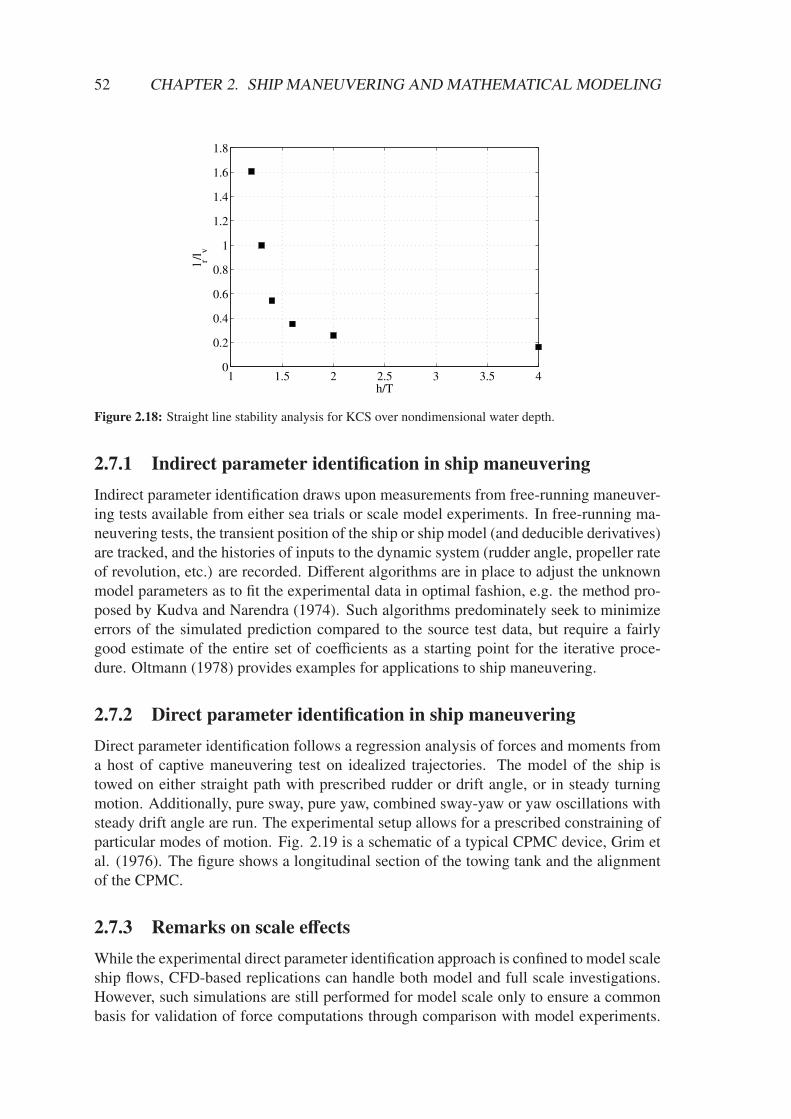
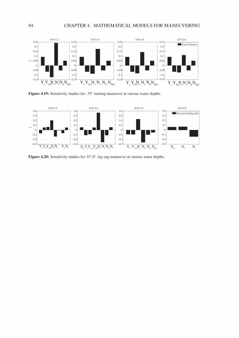
4.16 Zig-zag maneuver phase diagrams at various water depths I . . . . . . . . 924.17 Zig-zag maneuver phase diagrams at various water depths II . . . . . . . 934.18 Spiral curves of zig-zag maneuvers in shallow water . . . . . . . . . . . . 934.19 Sensitivity studies for a turning maneuver at various water depths . . . . . 944.20 Sensitivity studies for a zig-zag maneuver at various water depths . . . . 94
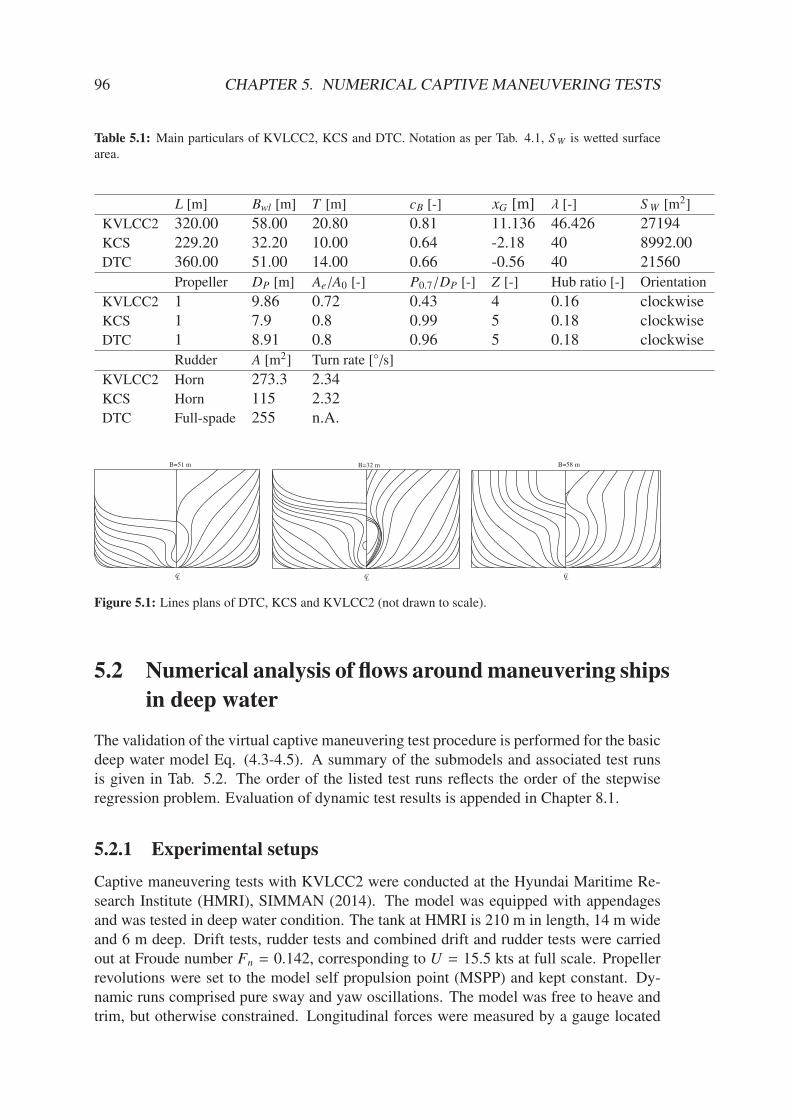
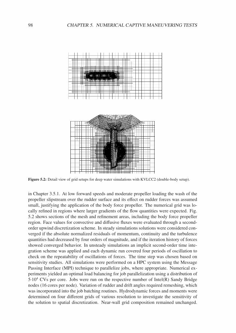
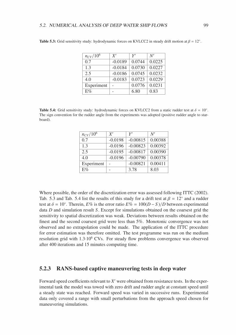
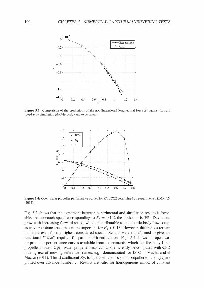
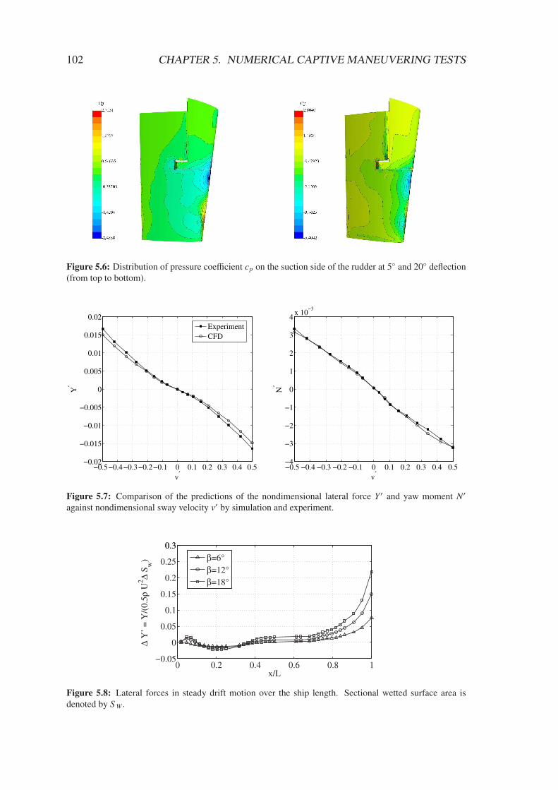
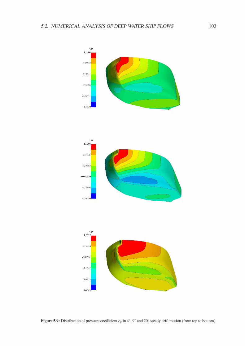
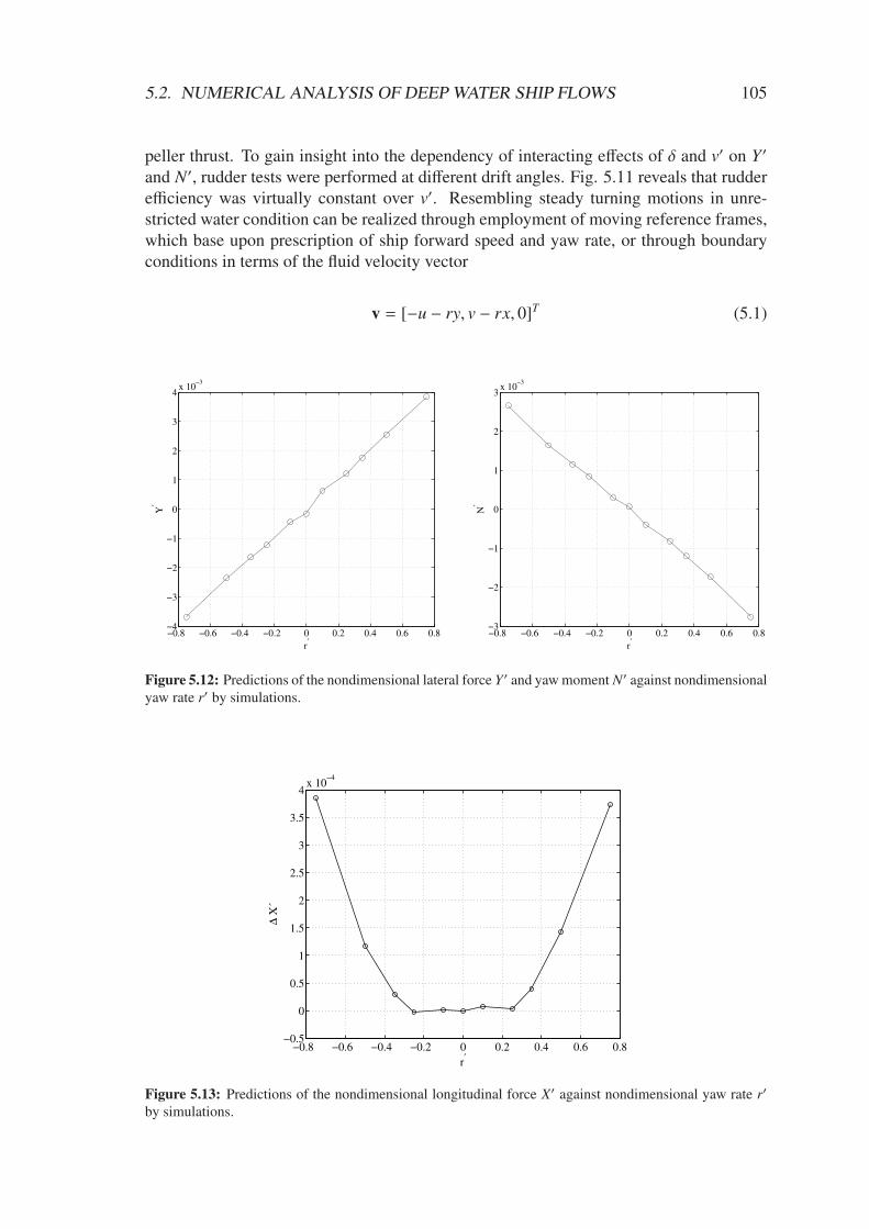
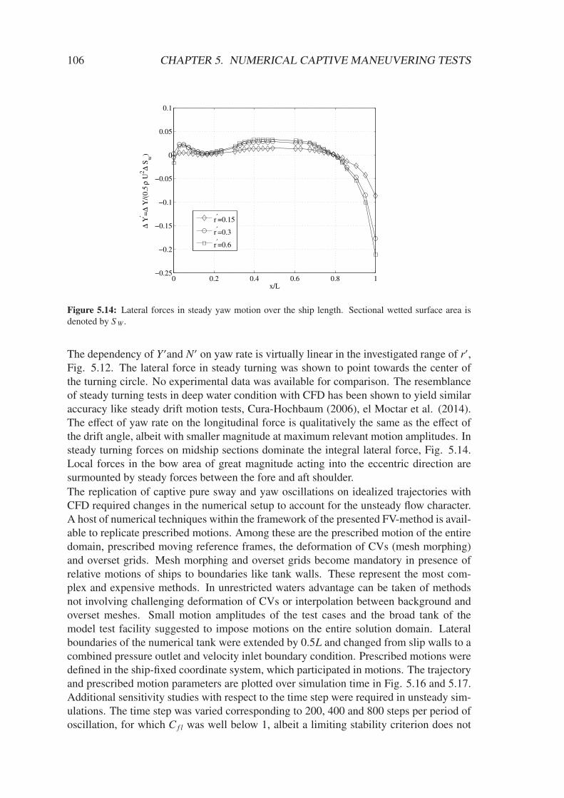
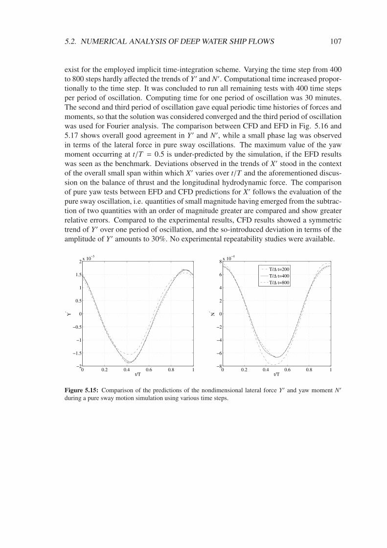
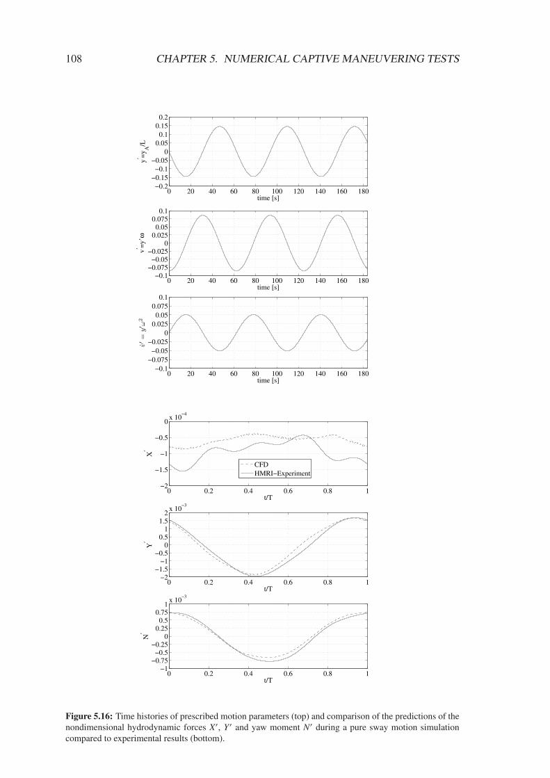
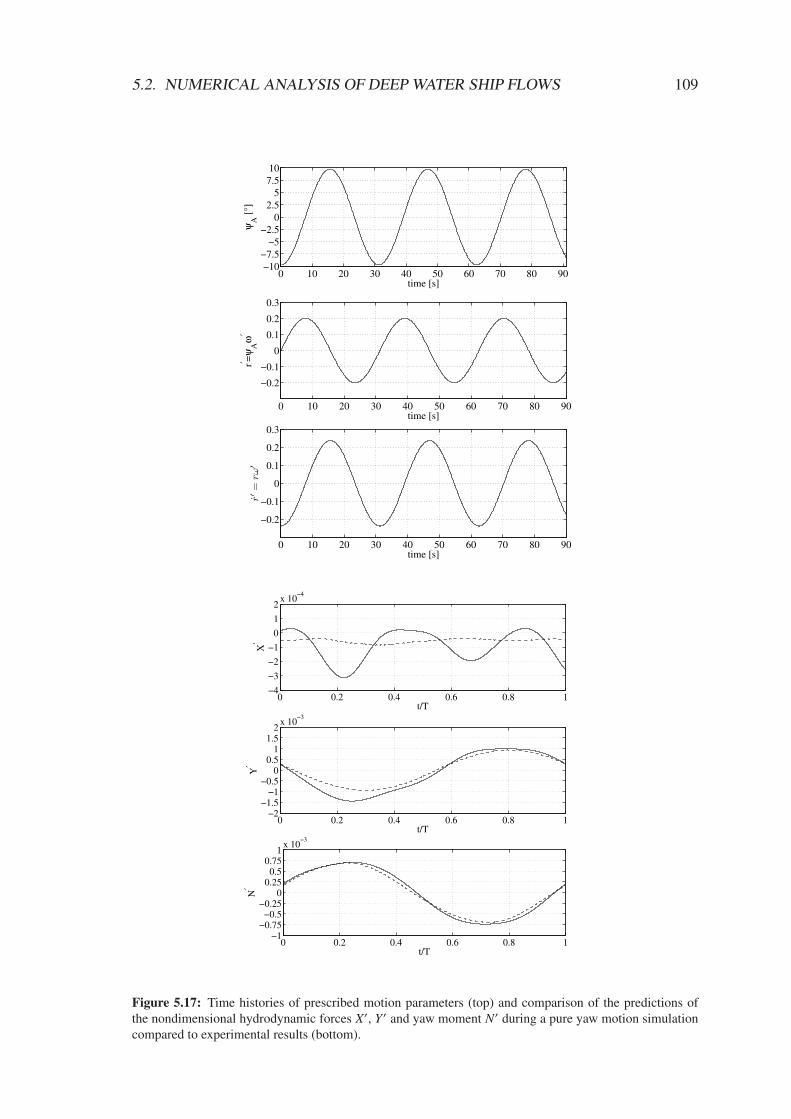
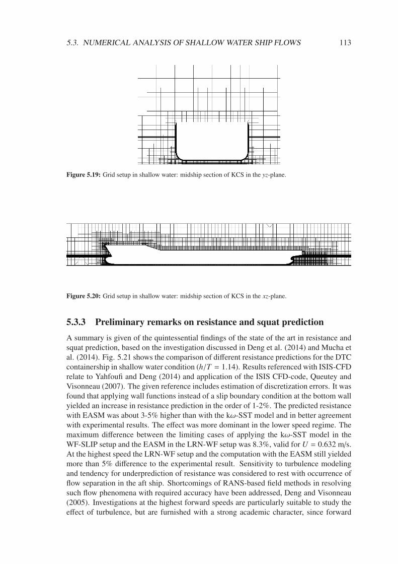
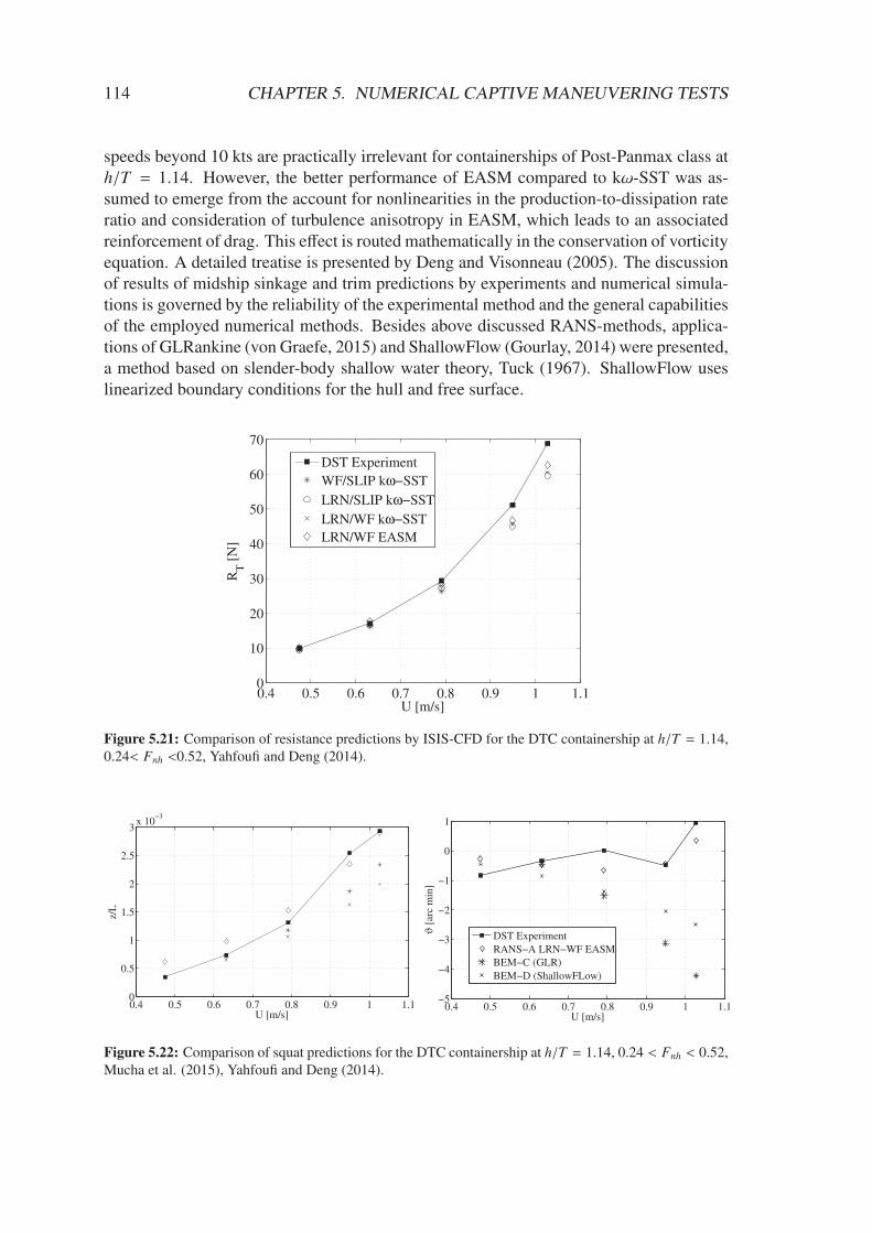
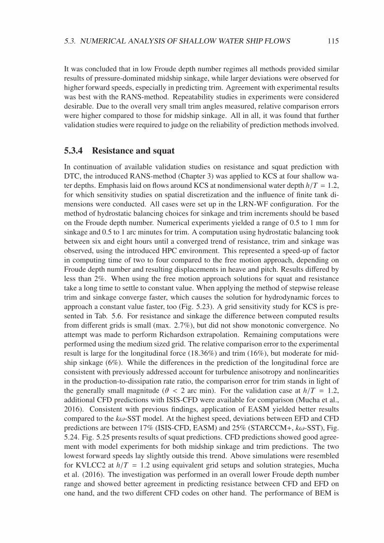
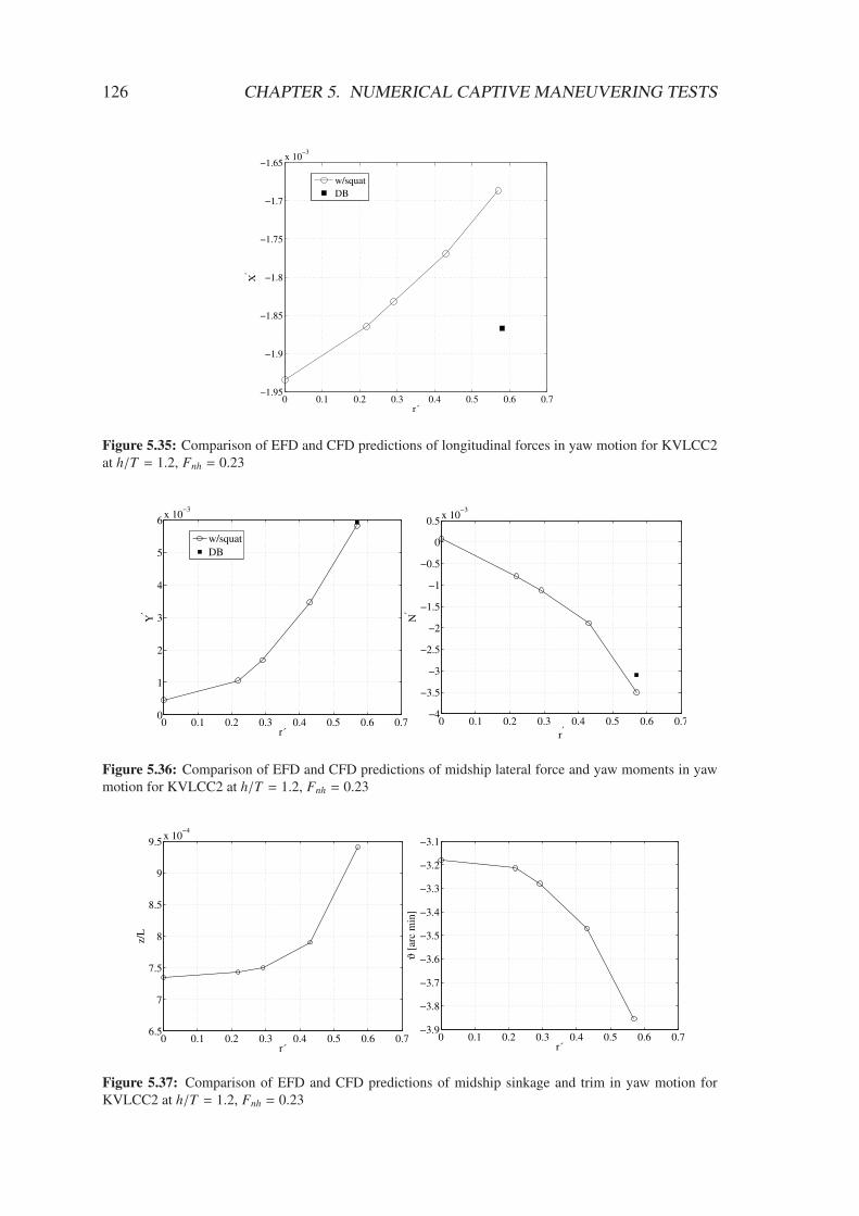
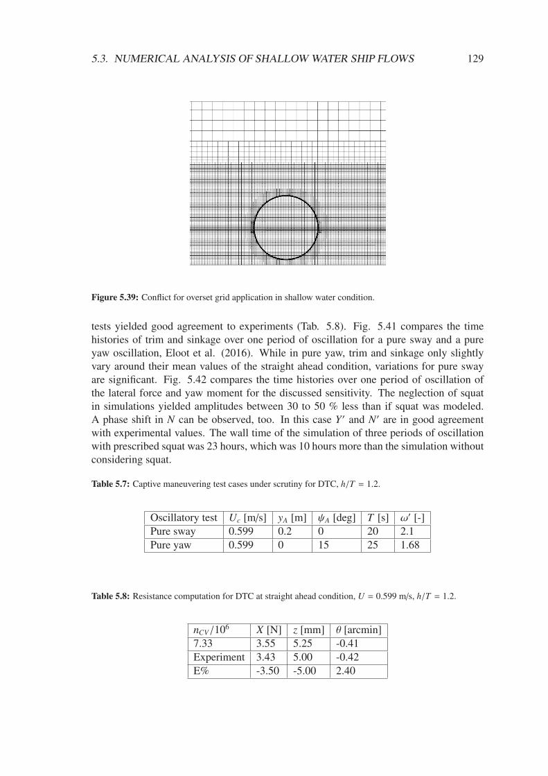
5.1 Lines plans of DTC, KCS and KVLCC2 . . . . . . . . . . . . . . . . . . 965.2 Detail view of grid setups for deep water simulations with KVLCC2 . . . 985.3 Resistance tests in deep water . . . . . . . . . . . . . . . . . . . . . . . . 1005.4 Propeller performance curves in deep water . . . . . . . . . . . . . . . . 1005.5 Rudder tests in deep water . . . . . . . . . . . . . . . . . . . . . . . . . 1015.6 Distribution of the pressure coefficient over the rudder surface . . . . . . 1025.7 Drift tests in deep water . . . . . . . . . . . . . . . . . . . . . . . . . . . 1025.8 Forces on segmented model in drift motion . . . . . . . . . . . . . . . . 1025.9 Distribution of the pressure coefficient over the hull in drift motion . . . . 1035.10 Drift and rudder tests in deep water I . . . . . . . . . . . . . . . . . . . . 1045.11 Drift and rudder tests in deep water II . . . . . . . . . . . . . . . . . . . 1045.12 Yaw tests in deep water I . . . . . . . . . . . . . . . . . . . . . . . . . . 1055.13 Yaw test in deep water II . . . . . . . . . . . . . . . . . . . . . . . . . . 1055.14 Forces on segmented model in yaw motion . . . . . . . . . . . . . . . . . 1065.15 Pure sway motion test in deep water I . . . . . . . . . . . . . . . . . . . 1075.16 Pure sway motion test in deep water II . . . . . . . . . . . . . . . . . . . 1085.17 Pure yaw motion test in deep water . . . . . . . . . . . . . . . . . . . . . 1095.18 Yaw with drift tests in deep water . . . . . . . . . . . . . . . . . . . . . . 1105.19 Grid setup in shallow water I . . . . . . . . . . . . . . . . . . . . . . . . 1135.20 Grid setup in shallow water II . . . . . . . . . . . . . . . . . . . . . . . . 1135.21 Shallow water resistance predictions for DTC . . . . . . . . . . . . . . . 1145.22 Shallow water squat predictions for DTC . . . . . . . . . . . . . . . . . . 1145.23 Resistance predictions in shallow water . . . . . . . . . . . . . . . . . . 1165.24 Resistance predictions in shallow water . . . . . . . . . . . . . . . . . . 1175.25 Squat predictions in shallow water . . . . . . . . . . . . . . . . . . . . . 1175.26 Scalar plots of wakes at different h/T . . . . . . . . . . . . . . . . . . . 1185.27 Detail view of free surface panels and triangular panels on the hull of KCS. 1195.28 Influence of squat on resistance . . . . . . . . . . . . . . . . . . . . . . . 1205.29 Analysis of friction resistance in various shallow water conditions. . . . . 1215.30 Longitudinal forces in drift motion in shallow water . . . . . . . . . . . . 1225.31 Forces in drift motion in shallow water . . . . . . . . . . . . . . . . . . . 1225.32 Squat in drift motion in shallow water . . . . . . . . . . . . . . . . . . . 1225.33 Squat effect on free surface elevation . . . . . . . . . . . . . . . . . . . . 1235.34 Lateral forces over segmented ship length of KCS. . . . . . . . . . . . . 1245.35 Longitudinal forces in yaw motion in shallow water . . . . . . . . . . . . 1265.36 Forces in yaw motion in shallow water . . . . . . . . . . . . . . . . . . . 1265.37 Squat in yaw motion in shallow water . . . . . . . . . . . . . . . . . . . 1265.38 Conflict for mesh morphing in shallow water condition . . . . . . . . . . 1285.39 Conflict for overset grid application in shallow water condition. . . . . . . 1295.40 Time histories of squat during captive maneuvering experiments with DTC 130
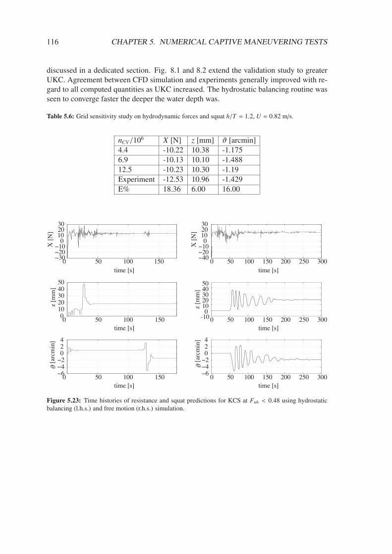
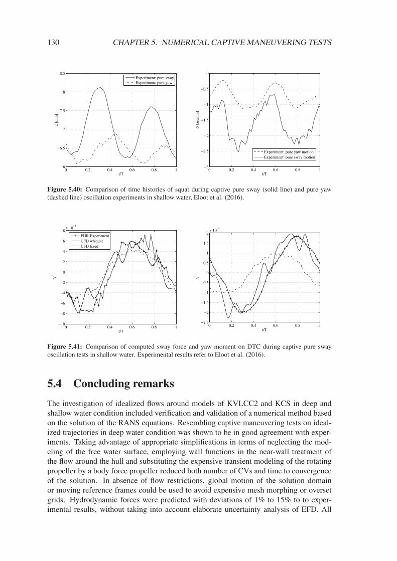
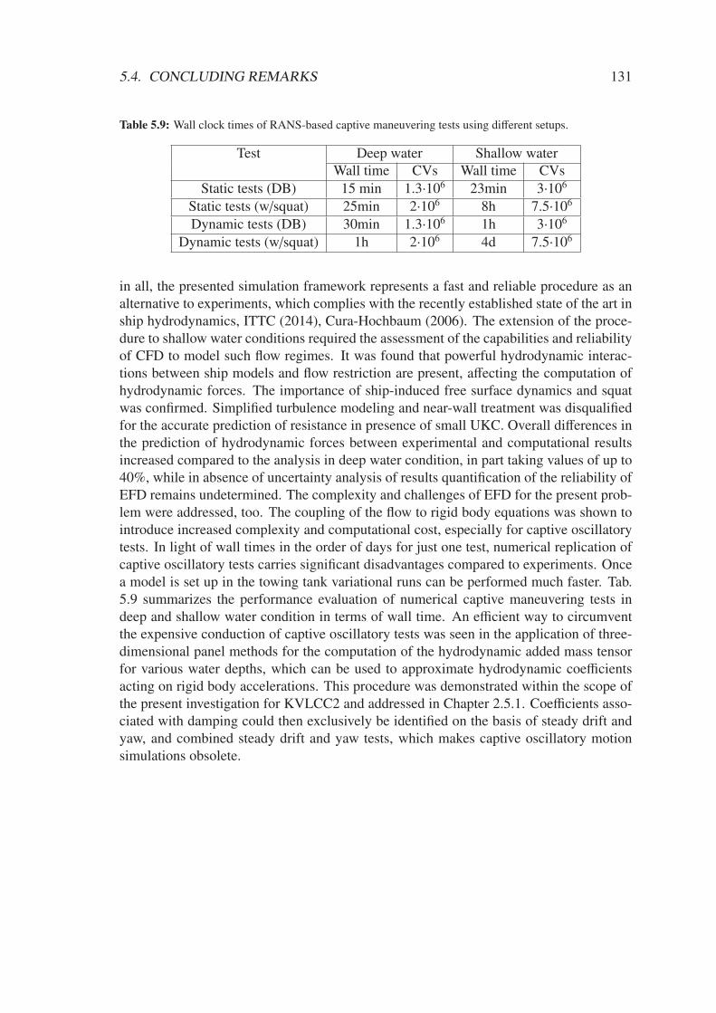
5.41 Influence of squat on hydrodynamic forces in captive maneuvering tests . 130
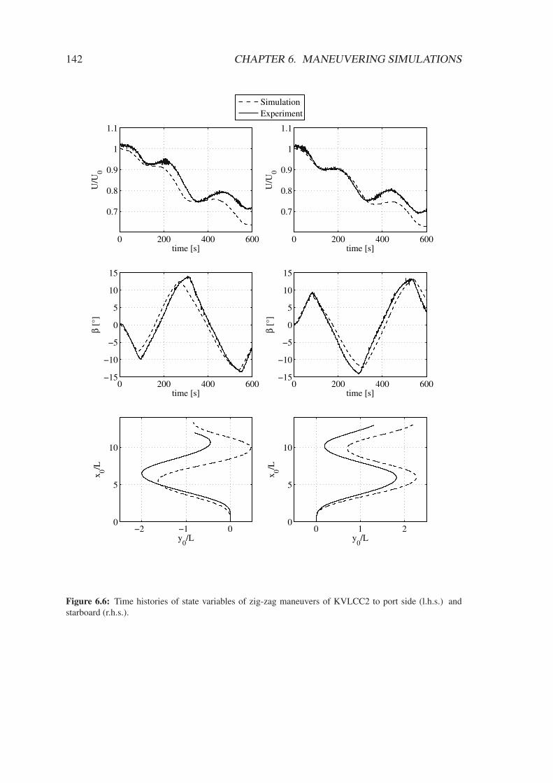
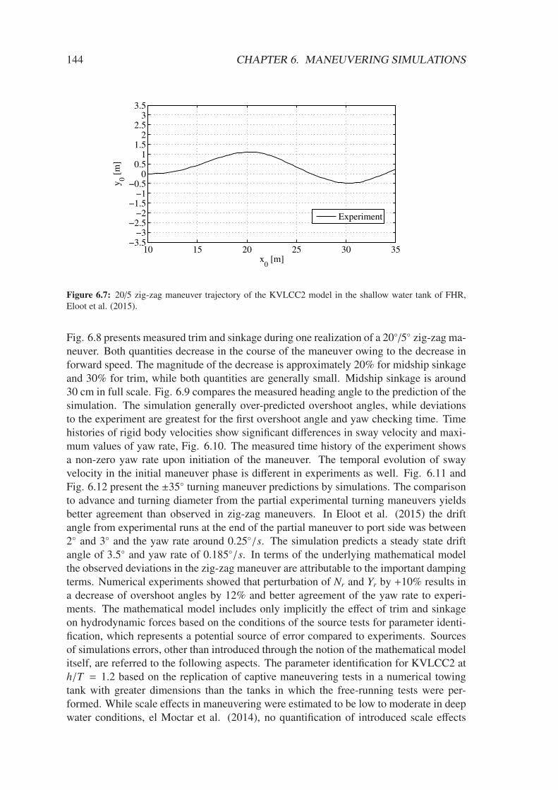
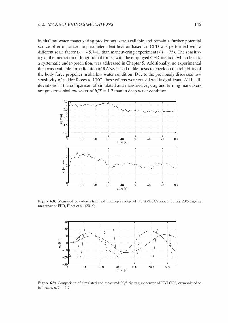
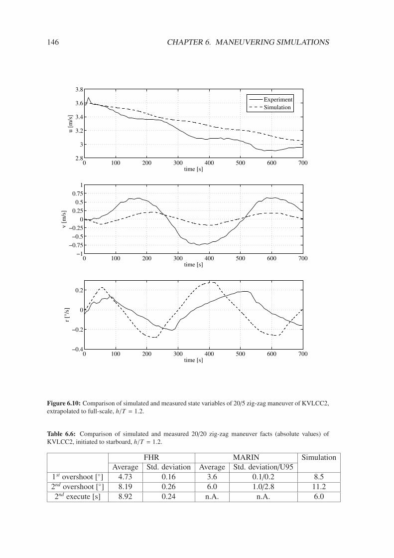
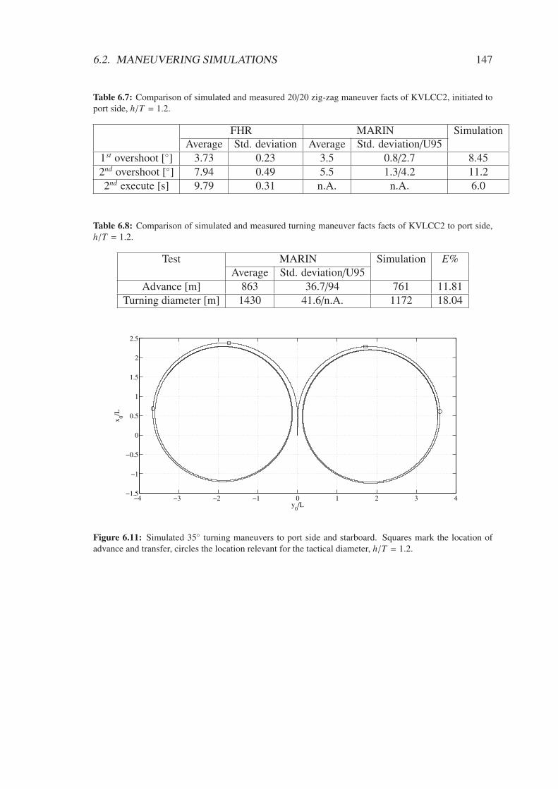
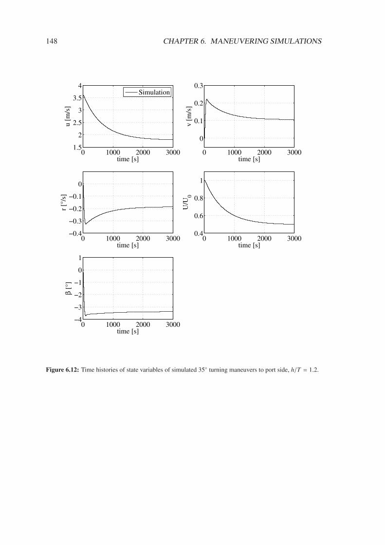
6.1 Turning maneuver study of KVLCC2 in deep water I . . . . . . . . . . . 1366.2 Turning maneuver study of KVLCC2 in deep water II . . . . . . . . . . . 1386.3 Turning maneuver study of KVLCC2 in deep water III . . . . . . . . . . 1396.4 Zig-zag maneuver study of KVLCC2 in deep water I . . . . . . . . . . . 1406.5 Zig-zag maneuver study of KVLCC2 in deep water II . . . . . . . . . . . 1416.6 Zig-zag maneuver study of KVLCC2 in deep water III . . . . . . . . . . 1426.7 Zig-zag maneuver trajectory in shallow water . . . . . . . . . . . . . . . 1446.8 Squat during zig-zag maneuver in shallow water . . . . . . . . . . . . . . 1456.9 Zig-zag maneuver study of KVLCC2 in shallow water I . . . . . . . . . . 1456.10 Zig-zag maneuver study of KVLCC2 in shallow water II . . . . . . . . . 1466.11 Turning maneuver of KVLCC2 in shallow water I . . . . . . . . . . . . . 1476.12 Turning maneuver of KVLCC2 in shallow water II . . . . . . . . . . . . 148
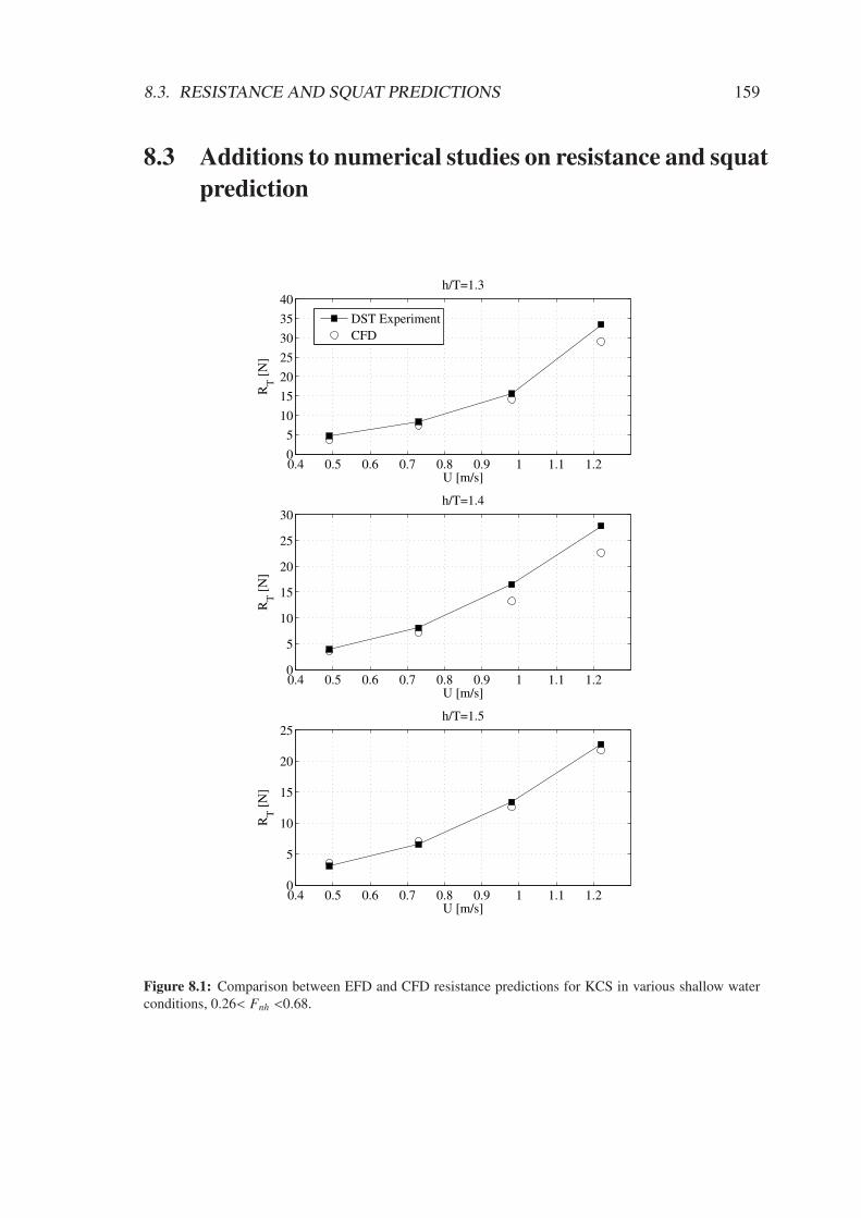
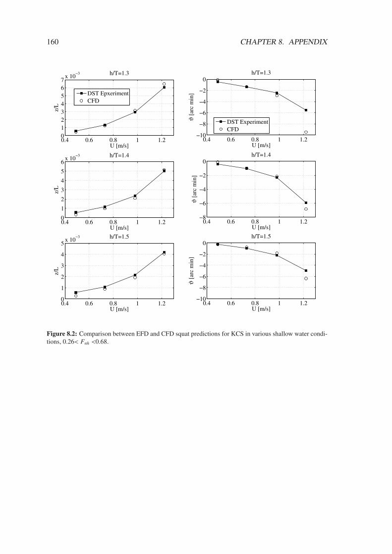
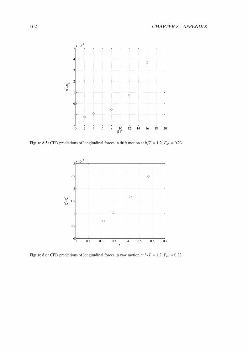
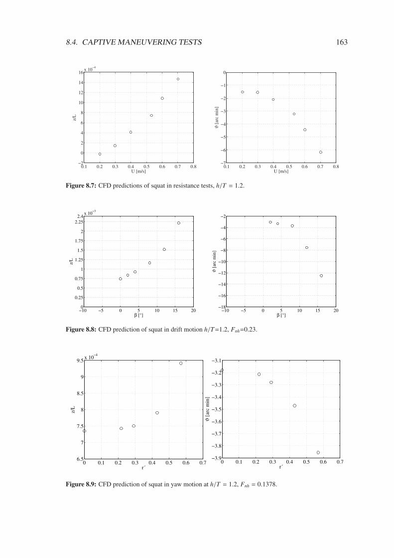
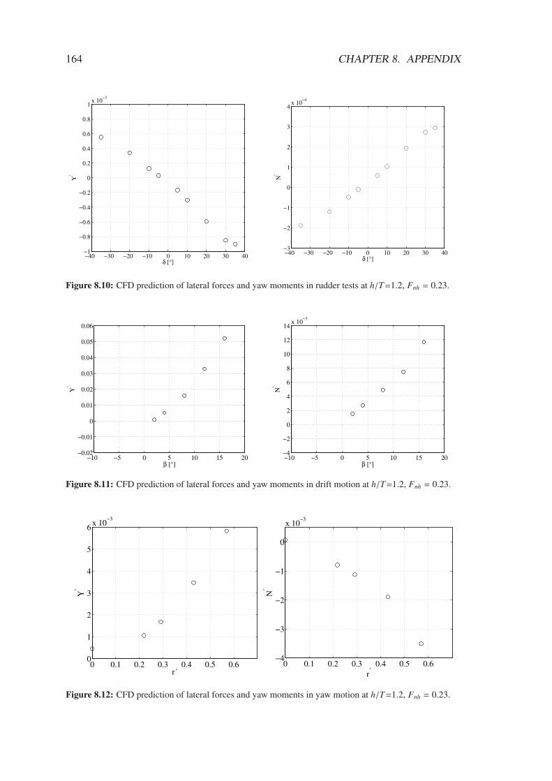
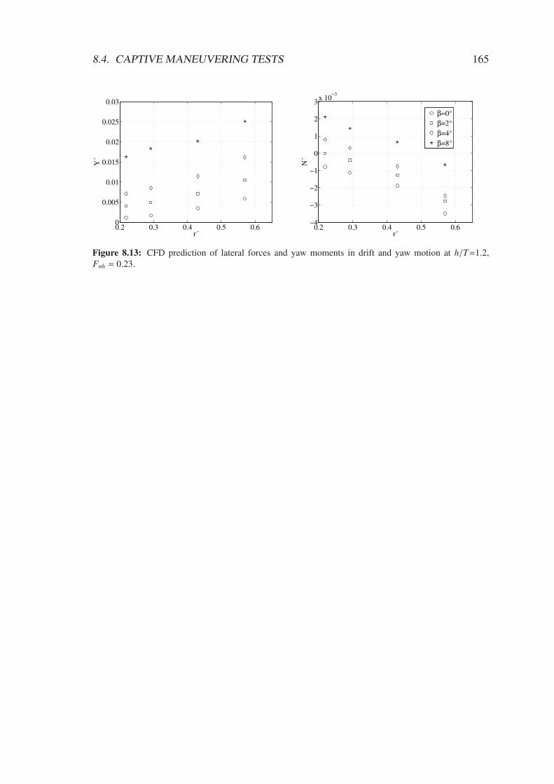
8.1 Resistance predictions in various shallow water conditions . . . . . . . . 1598.2 Squat predictions in various shallow water conditions . . . . . . . . . . . 1608.3 Shallow water resistance prediction . . . . . . . . . . . . . . . . . . . . 1618.4 Longitudinal forces in rudder tests in shallow water . . . . . . . . . . . . 1618.5 Longitudinal forces drift motion in shallow water . . . . . . . . . . . . . 1628.6 Longitudinal forces yaw motion in shallow water . . . . . . . . . . . . . 1628.7 Shallow water squat prediction . . . . . . . . . . . . . . . . . . . . . . . 1638.8 Forces in rudder tests in shallow water . . . . . . . . . . . . . . . . . . . 1638.9 Squat in yaw motion in shallow water . . . . . . . . . . . . . . . . . . . 1638.10 Forces in rudder tests in shallow water . . . . . . . . . . . . . . . . . . . 1648.11 Forces in drift tests in shallow water . . . . . . . . . . . . . . . . . . . . 1648.12 Forces in yaw motion in shallow water . . . . . . . . . . . . . . . . . . . 1648.13 Forces in rudder tests in shallow water . . . . . . . . . . . . . . . . . . . 165
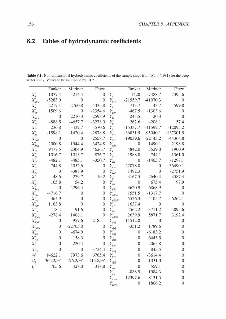
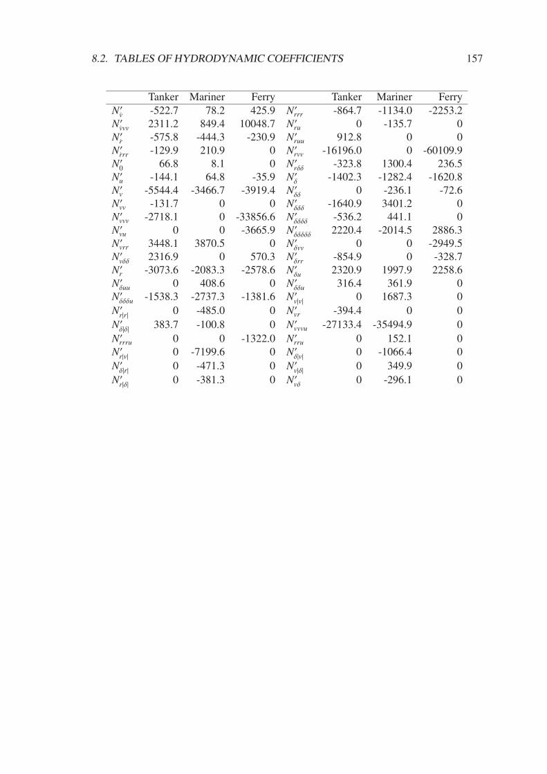
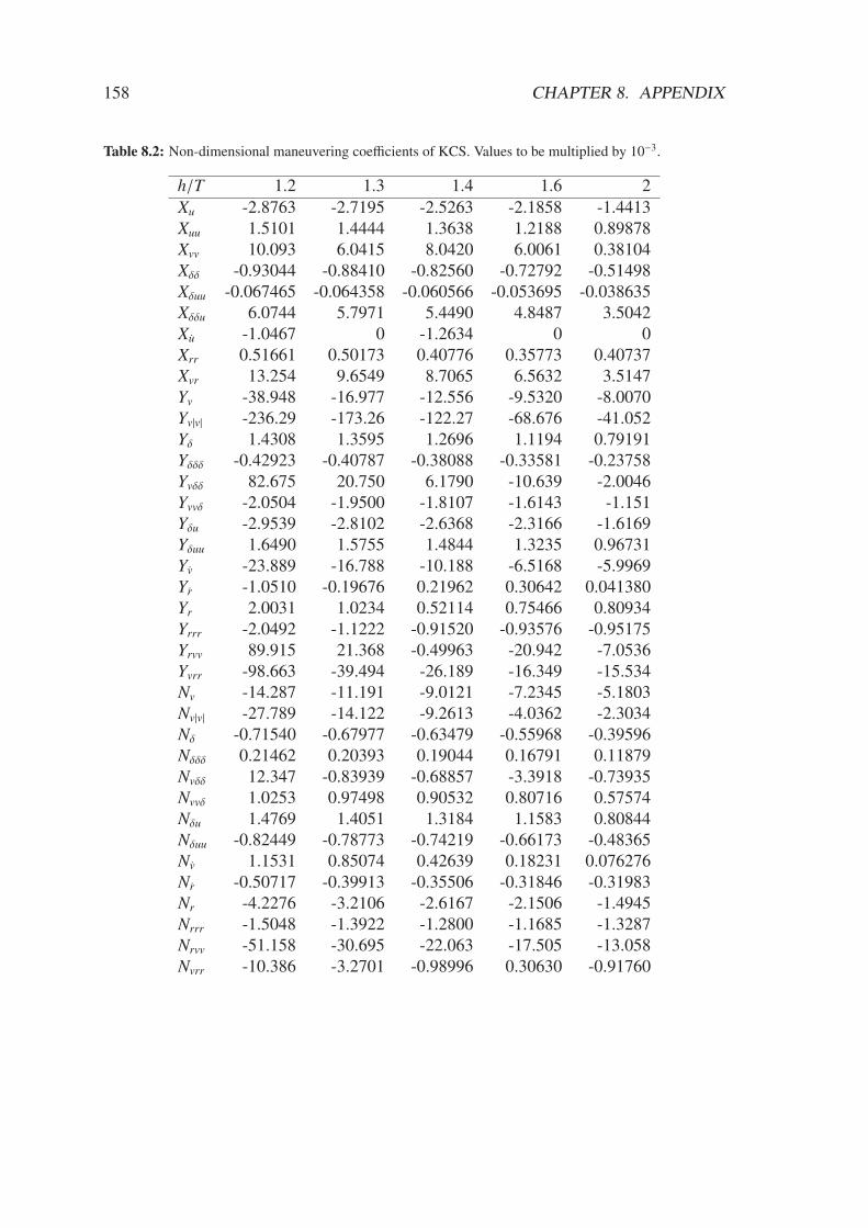
List of Tables
2.1 Number of test runs in experimental designs . . . . . . . . . . . . . . . . 57
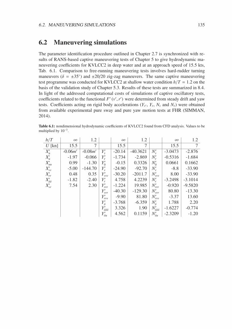
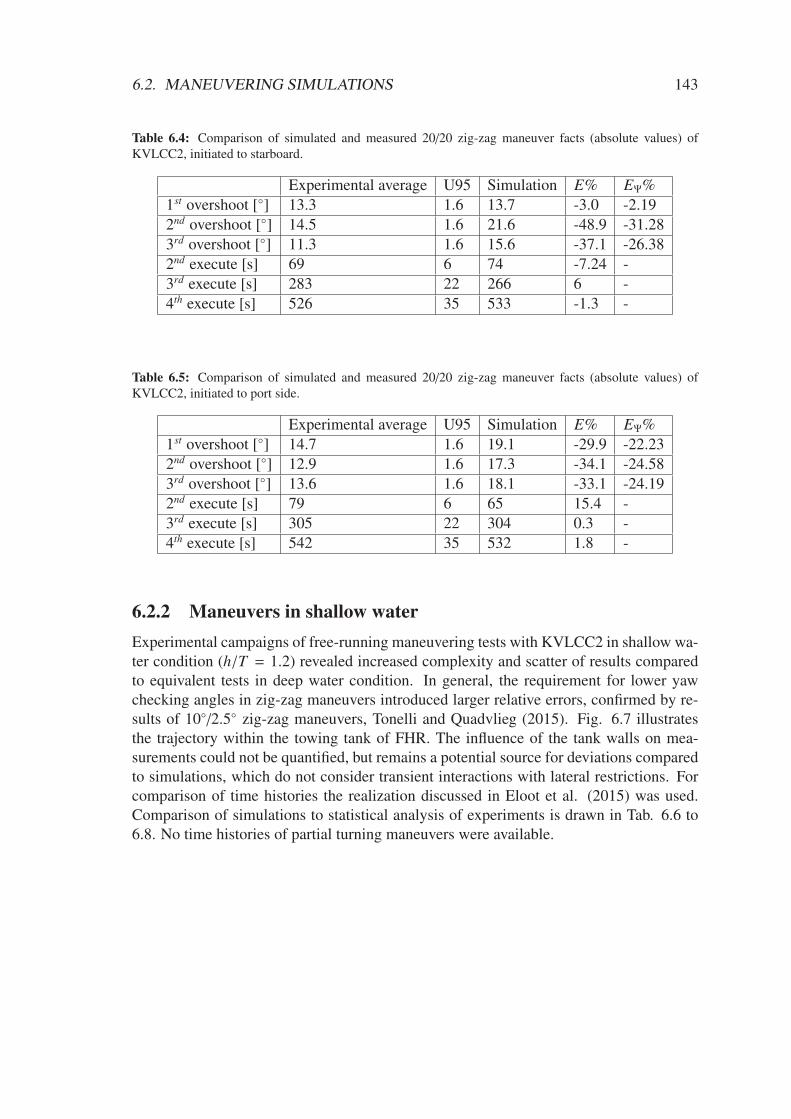
6.1 Table of hydrodynamic coefficients of KVLCC2 . . . . . . . . . . . . . . 1356.2 Turning maneuver study of KVLCC2 in deep water IV . . . . . . . . . . 1376.3 Turning maneuver study of KVLCC2 in deep water V . . . . . . . . . . . 1376.4 Zig-zag maneuver study of KVLCC2 in deep water IV . . . . . . . . . . 1436.5 Zig-zag maneuver study of KVLCC2 in deep water IV . . . . . . . . . . 1436.6 Zig-zag maneuver study of KVLCC2 in shallow water facts I . . . . . . . 1466.7 Zig-zag maneuver in shallow water facts II . . . . . . . . . . . . . . . . . 1476.8 Turning maneuver of KVLCC2 in shallow water III . . . . . . . . . . . . 147
The prediction of maneuverability is a classic problem in ship hydrodynamics. Likewise,ship motions in restricted waters have been studied for a long time. In the open sea, wherethe major part of ship journeys takes place, the focus lies on the prediction of propulsioncharacteristics and wave-induced motions in stochastic environments. Ship maneuvering,however, is relevant in coastal areas and harbor approaches, where space is limited, traf-fic heavier, and where hydrodynamic interaction effects are present, increasing hazards.The renewed attention referred to maneuvering prediction in general, and its extensionto restricted waters in particular, is attributable to three trends. First, ships are becomingbigger in size while existing waterways are not growing at the same pace. Consequently,waterway administrations are strongly interested in ship motion predictions in the contextof the entering of ports and channel systems. Further incentives emerge from the applica-tion of ship handling simulators, which widely come into operation for training of nauticalstaff, but which are increasingly being used for navigability analyses too. Such investiga-tions require accurate modeling of ship motions and validation of simulations. Second,a novel regulatory framework following the call for green shipping brings attention tominimum power requirement estimation to ensure safe and economic ship operation inadverse conditions. In light of an expected trend towards an overall decrease in powerinstallation, predictions of wave and shallow water impacts on maneuvering performanceare needed for the design of efficient and safely operable ships. Third, numerical meth-ods and computational resources have advanced to turn simulation-based analyses of shipflows into a competitive alternative to experiments. While models for ship maneuvering inshallow water have been proposed and investigated based on experimental fluid dynamics,little is known about the performance and reliability of entirely simulation-based meth-ods. The complexity of the task rests with the modeling of turbulence, free surface effectsand rigid body motions. Among the latter particular attention is directed to ship squat.Computational Fluid Dynamics (CFD) is meanwhile applicable to a host of problemsin ship hydrodynamics, including maneuvering. The solution of the Reynolds-averagedNavier-Stokes (RANS) equations is the predominate choice for CFD applications in shiphydrodynamics. Yet, the need exists for further assessment of reliability, especially forshallow water problems. Notwithstanding the advance of CFD, potential flow methodsstill embody a valuable and cost-efficient tool for hydrodynamic analyses. Against thebackground of an anticipated increasing relevance of viscous effects in restricted water itis desirable to explore performance, prospects and limitations of such numerical methods.
18 CHAPTER 1. INTRODUCTION
1.1 State of the art in ship maneuvering prediction
The study of ship maneuverability started with the invention and use of surface vessels,because ship pilots and designers were interested in the response characteristics to com-manded changes of the direction of ship motions, which ties in with the fundamental defi-nition of maneuvering given in the Principles of Naval Architecture (PNA), Mandel (1965)and Crane et al. (1989). Over millennia the role of ships in trade, transport, warfare andleisure has continuously become more important; and so did the interest in performanceestimation and improvement increase. A compact summary of the scientific dedication tothe problem of maneuverability analysis up to the mid-1960s is given in Newman (1966).A more comprehensive treatment of the recent history of related research can be foundin Sutulo and Guedes Soares (2011). Practical aspects of ship maneuverability are abun-dantly covered by Brix (1993). A notable work towards the formulation of mathematicalmodels for maneuvering prediction is presented in Davidson and Schiff (1946), who de-rived a linear framework of ship maneuvering equations of motion in the horizontal plane.Nomoto et al. (1957) discussed a model for dynamics in yaw, which has widely been ap-plied to heading control problems. Successive investigations and developments towardsnonlinear extensions are related to Norrbin (1960) or Wagner-Smith (1971). An impor-tant contribution to the mathematical modeling of maneuvering is referred to Abkowitz(1964), who formulated maneuvering equations in six degree-of-freedom (DoF) based onmodified Taylor-series expansions of functionals of hydrodynamic forces. Such modelsuse multivariat algebraic polynomials to account for dependencies of forces on rigid bodymotions and control surface variables and involve a host of coefficients describing hydro-dynamic properties. Above introduced ideas of Abkowitz (1964) received great attentionin the hydrodynamic community with the introduction of mechanic oscillators at exper-imental facilities, which started at David Taylor Model Basin (DTMB), Gertler (1959),Goodman (1966). Such devices, which came to be called Planar Motion Mechanisms(PMM), enabled prescribed and captive motions of ship models in towing tanks, whichcould be used to study motions relevant for maneuvering, e.g. pure sway or pure yawoscillations. Evaluation of such tests with respect to identification of maneuvering co-efficients is covered in Strøm-Tejsen and Chislett (1966). A facility for planar motiontesting of ship models arose in Hamburg, Germany, in the context of the joint researchpool for shipbuilding, designated Sonderforschungsbereich Schiffbau 98 (SFB 98), Grimet al. (1976). The particular device installed was a Computerized Planar Motion Car-riage (CPMC), which enabled large amplitude motions with high precision in trajectoryprescription and measurement. Main contributions to mathematical modeling of maneu-vering within SFB 98 relate to Oltmann and Sharma (1984) and Wolff (1981). Oltmann(1978), Oltmann and Wolff (1979) and Wolff (1981) discussed the operation of the CPMCfor captive and free-running maneuvering tests and synchronization of results for systemidentification of maneuvering models. Fedajevski and Sobolev (1964) discussed the mod-eling of hydrodynamic damping forces by second-order modulus functions based on thehydrodynamic drag concept, which was later extended by Hooft (1994). Widely refer-enced contributions refer to the Japanese Maneuvering Modeling Group (JMMG, Ogawa,1977), e.g. Inoue (1981), Yasukawa and Yoshimura (2014). Models proposed by JMMGdraw upon decomposed formulations of force effects and application of experiments, the-ory and empirics to identify emerging maneuvering coefficients. The use of slender-body
1.2. STATE OF THE ART 19
theory in the ship maneuvering context is covered by Newman (1978) and Söding (1982c).Important theoretical contributions on consideration of time-dependent modeling of shipmotions accounting for fluid memory effects were made by Cummins (1962) and Ogilvie(1964). A broad overview of established maneuvering models tailored to different appli-cation domains is given in Fossen (2011). Full-scale maneuvering sea trials have beenthe method of choice to analyze maneuvering performance in absence of computationalmethods and experiments and are practically relevant for maneuvering criteria by the In-ternational Maritime Organisation (IMO), MSC 137(76) (2002). Published reports in-cluding results for validation purposes for the Mariner standard ship and a tanker relateto Morse and Price (1961) and Ogawa (1971). The advance of computational methodsand the increase in computational power enabled numerical studies into ship flows aroundmaneuvering ships using CFD. While initially valuable insight into steady drift and yawmotions, as well as rudder forces was gained, Sato (1998) and el Moctar (2001a, 2001b),such methods were soon able to replicate captive model tests, and it became feasibleto derive maneuvering coefficients with CFD, Cura-Hochbaum (2006). Applications tomaneuvering prediction in deep water were verified and validated in the SIMMAN work-shop, Stern et al. (2011). Primary investigations were confined to double-body flows.More complex cases involving the modeling of the free surface and ship motions weredealt with preliminary only in deep water conditions. Recently, direct CFD simulationsof rudder maneuvers were performed, which model the appended hull geometry and re-solve ship motions transiently, using available numerical techniques for consideration ofpropeller and rudder motions. These simulations are time-consuming and rendered in-feasible for parametric investigations. Only few publications are available, Carrica et al.(2013), Mofidi and Carrica (2014), el Moctar et al. (2014). A general evaluation of capa-bilities and prospects of CFD can be found in Larsson and Bertram (2003) and Larssonet al. (2013). A regular survey of related research activities is done by the ManeuveringCommittee of the International Towing Tank Conference (ITTC, 2014).
1.2 State of the art in ship hydrodynamics in restricted
waters
Weinblum (1934), Brard (1951), Schuster (1952) and Silverstein (1957) addressed theissue of ship motions in shallow water relatively early compared to the treatise of maneu-vering in deep water. Prediction of shallow water effects on forward motion, involving thechange in ship resistance and consideration of squat, was notably dealt with by Kreitner(1934), Havelock (1939) and Thews and Landweber (1935). The summary of Tuck (1978)is a comprehensive dedication to ship hydrodynamic problems encountered in restrictedwaters. The attention in research was mainly drawn to the prediction of ship-induced shal-low water waves, the formulation of forces on the hull in presence of vertical and lateralrestrictions and consequences for ship motions. Shallow water ship waves were studied byChen (1999), Chen and Sharma (1995), Sharma and Chen (2000) and Jiang (2003) usingdepth-averaged flow equations of Boussinesq-type. Notable contributions in conjunctionwith ship-induced shallow water waves also relate to Li and Sclavounos (2002) and Alamand Mei (2008). In response to parallel developments and better understanding of slender-body theory for the formulation of ship motions in deep water, Tuck (1963, 1966, 1967)
20 CHAPTER 1. INTRODUCTION
and Tuck and Taylor (1970) studied the extension of the mathematical framework to finitewater depth. Newman (1969), Beck et al. (1975), Beck (1977), Breslin (1972) and Nor-rbin (1971) studied forces on ships in channels using slender-body theory. Zhao (1986)presented related applications to ship maneuvering in shallow water and included compar-isons to experimental studies by Fujino (1968, 1972, 1984). Interaction effects with banksand ships are addressed in Tuck and Newman (1978), who developed formulations of thesway force and yaw moment for two bodies moving on a parallel path for the shallow anddeep water case, and Yeung (1978). Söding (2005) presented the study of overtaking ma-neuvers with panel methods, which are extended in von Graefe (2015). Straight line sta-bility and control related problems in restricted waters leaning on hydrodynamic analysiswith a Rankine panel method were discussed in Thomas and Sclavounos (2006). Norrbin(1971) discussed consequences of finite water depth for mathematical models for maneu-vering. Inoue (1969) studied linear and nonlinear lifting theory applied to flows aroundships in shallow water on the basis of the ideas presented in Bollay (1936). Systematicexperimental investigations on the influence of water depth and consequences for variousmathematical maneuvering models were performed by Fujino (1968) and Gronarz (1993,1997). Experimental studies on ship-ship interaction and bank-effects were performed byVantorre et al. (2002), Eloot and Vantorre (2009) and Lataire and Vantorre (2008). Elootet al. (2015) and Tonelli and Quadvlieg (2015) reported on efforts of validation of shal-low water maneuvering simulations through free-running experiments. The prediction ofsquat is of paramount importance in under-keel clearance (UKC) management for shipsand has been receiving great attention in the hydrodynamic community. Definition of ter-minology is provided by Tuck (1978). Gourlay (2000, 2001, 2006, 2008, 2011) appliedTuck’s theories to a host of squat problems. Millward (1992) summarized theoretical andempirical squat prediction methods. Graff et al. (1964) discussed a detailed study onsquat prediction through model experiments. Early application of CFD to lifting flows inshallow water was confined to inviscid or double-body simulations, neglecting both freesurface disturbances and squat, e.g. Gronarz (1997). Deng et al. (2014) represents arelevant contribution with respect to the reliability of CFD for application to squat and re-sistance predictions. Comparing investigations of different numerical methods are foundin Mucha and el Moctar (2014) and Mucha et al. (2014, 2016). A review of activitiesin the field is found in regular reports of the Manoeuvring Committee of ITTC and theproceedings of the International Conference on Ship Manouevring in Shallow and Con-fined Waters (MASHCON), e.g. Eloot and Vantorre (2009). Applications of CFD to flowsaround ships in shallow water have recently been addressed at MASHCON, Uliczka et al.(2016).
1.3 Objectives and organization of the thesis
The thesis at hand aims to assess the capabilities of a simulation-based framework forthe prediction of rudder maneuvers in deep and shallow water. It is organized accord-ing to three objectives. In a first step, a review of relevant established approaches tothe modeling of hydrodynamic forces in the maneuvering equations of motion was con-ducted. Particular attention was referred to coefficient-based mathematical models, whichare represented mathematically by a set of coupled nonlinear differential equations in the
1.3. OBJECTIVES AND ORGANIZATION OF THE THESIS 21
framework of Newtonian mechanics, and which draw upon the formulation of hydrody-namic forces in maneuvering through multivariat polynomials. The specific formulationof the model structure for the purposes of this thesis included the discussion and for-mulation of suitable parameter identification procedures for the emerging hydrodynamiccoefficients. The parameter identification method leaned on the performance of captivemaneuvering tests on idealized trajectories. Taking the perspective of the early stage ofship design, when generally no experimental data is available, such motivated simulationmethods allow systematic variations of water depth and synchronization with underlyingmathematical models and require only a three-dimensional virtual, geometric representa-tion of the ship. In a second step, the performance and reliability of a RANS-based CFDmethod for parameter identification was assessed through comparison with experiments.Special emphasis was laid on ship-induced free surface disturbances and the prediction ofthe decrease of UKC through dynamic sinkage and trim (squat), which was expected tobe important for the computation of forces and moments on maneuvering ships in shallowwater. Comparison was drawn to other numerical methods for hydrodynamic analyses. Ina third step, above framework was applied to maneuvering prediction on shallow water fora candidate ship and compared to available time responses of free-running maneuveringexperiments with scale models.
22 CHAPTER 1. INTRODUCTION
2. Theory of Ship Maneuvering and
Mathematical Modeling
This chapter introduces ship maneuverability and maneuvering theory constituting the ba-sis for the development of the simulation-based maneuvering prediction framework. Thediscussion of maneuverability includes a general definition, presentation of maneuveringrequirements and established methodology for evaluation purposes. Equations of motionof maneuvering ships are formulated through application of classic Newtonian mechanicsfor rigid bodies. The problem of modeling hydrodynamic forces in maneuvering is intro-duced. The discussion starts with deep water conditions and related established concepts.Following a general treatise of hydrodynamic effects on maneuvering in shallow water,these concepts are scrutinized in terms of their capabilities to take mathematical accountof these effects. Special attention is given to multivariat polynomial models. Suitableparameter identification procedures are addressed.
2.1 Definitions and frames of reference
An earth-fixed inertial reference frame OxOyOzO, defined by origin O and right-handedCartesian axes xO, yO, zO, is introduced. Origin O is located at the calm water level. AxesxO and yO are mutually perpendicular in the horizontal plane and zO points downwards.
X, xs, u
U
β
δ Y, ys, v
N, ψ , rΨ
x
y
Z, zs, w
K, φ, p
x
y
z
X, xs, u
Y, ys, v
N, ψ , r
O
O
O
O
O
O
OSS
M, ϑ, q
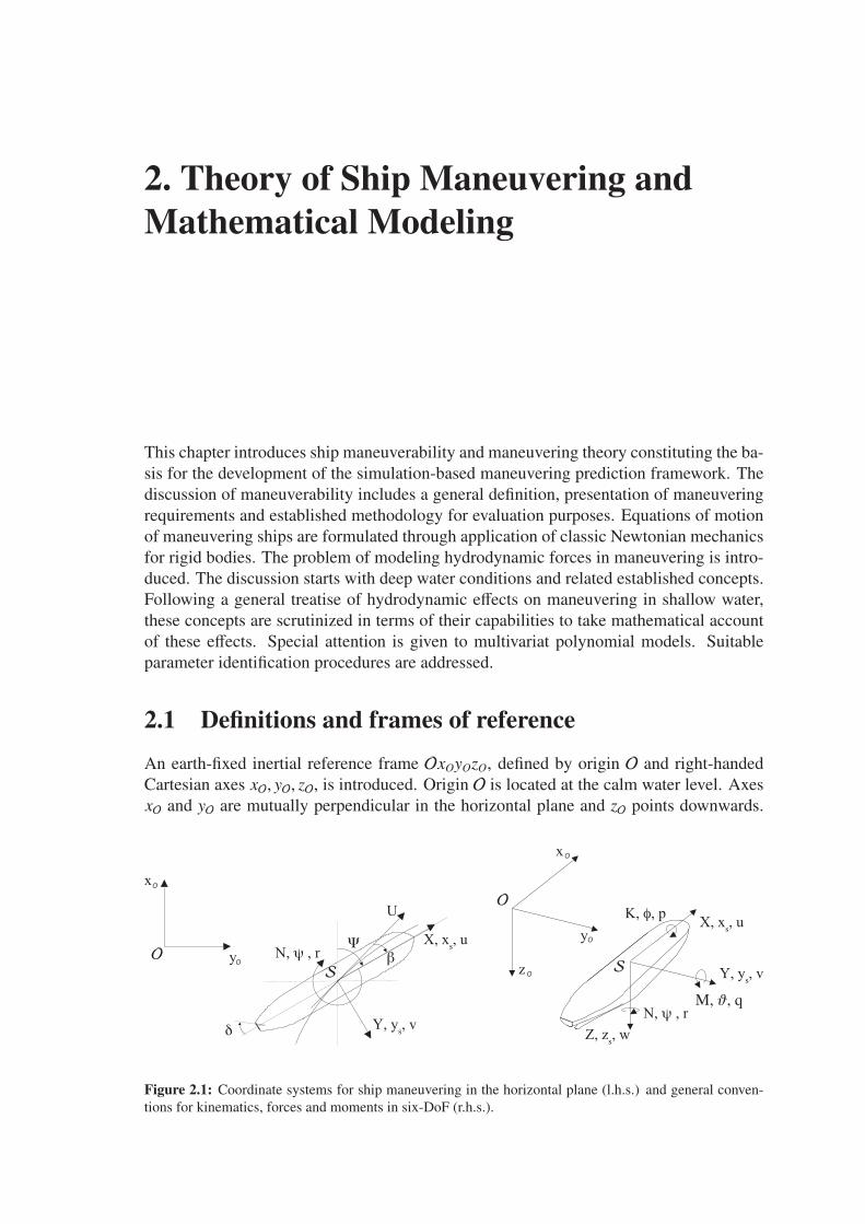
Figure 2.1: Coordinate systems for ship maneuvering in the horizontal plane (l.h.s.) and general conven-tions for kinematics, forces and moments in six-DoF (r.h.s.).
24 CHAPTER 2. SHIP MANEUVERING AND MATHEMATICAL MODELING
Additionally, a body-fixed reference frame Sxyz, defined by origin S and right-handedCartesian axes x, y, z, is used. Axis x points into the ship’s forward direction, lays inthe xy-plane of symmetry and coincides with the calm waterline. Axis y points posi-tively to starboard and axis z positively downward. Generalized coordinates of the shipare Cartesian coordinates xO, yO, zO in the earth-fixed frame, with generalized velocitiesVO =
[
xO, yO, zO]T , and with Eulerian anglea orientation φ (around x-axis), θ (around y-
axis) and ψ (around z-axis). Angular velocities are part of vector ΩO =[
φ, θ, ψ]T
. Inmaneuvering theory, it is common practice to use the projections of instantaneous groundvelocity vector V = [u, v,w]T and angular velocity vector Ω =
[
p, q, r]T onto the ship-
fixed reference frame Sxyz. The transformation between the reference systems conse-quently follows as per
and cφ = cos φ, cθ = cos θ, cψ = cosψ and sφ = sin φ, sθ = sin θ, sψ = sinψ. Consistentwith Fig. 2.1, instantaneous ship speed U in the xy-plane (w=0) is defined as
U =√
u2 + v2 (2.4)
and ship heading Ψ is related to the horizontal orientation of the ship with respect toOxOyO. Drift angle β is given by
β = arcsin (v/ − u) (2.5)
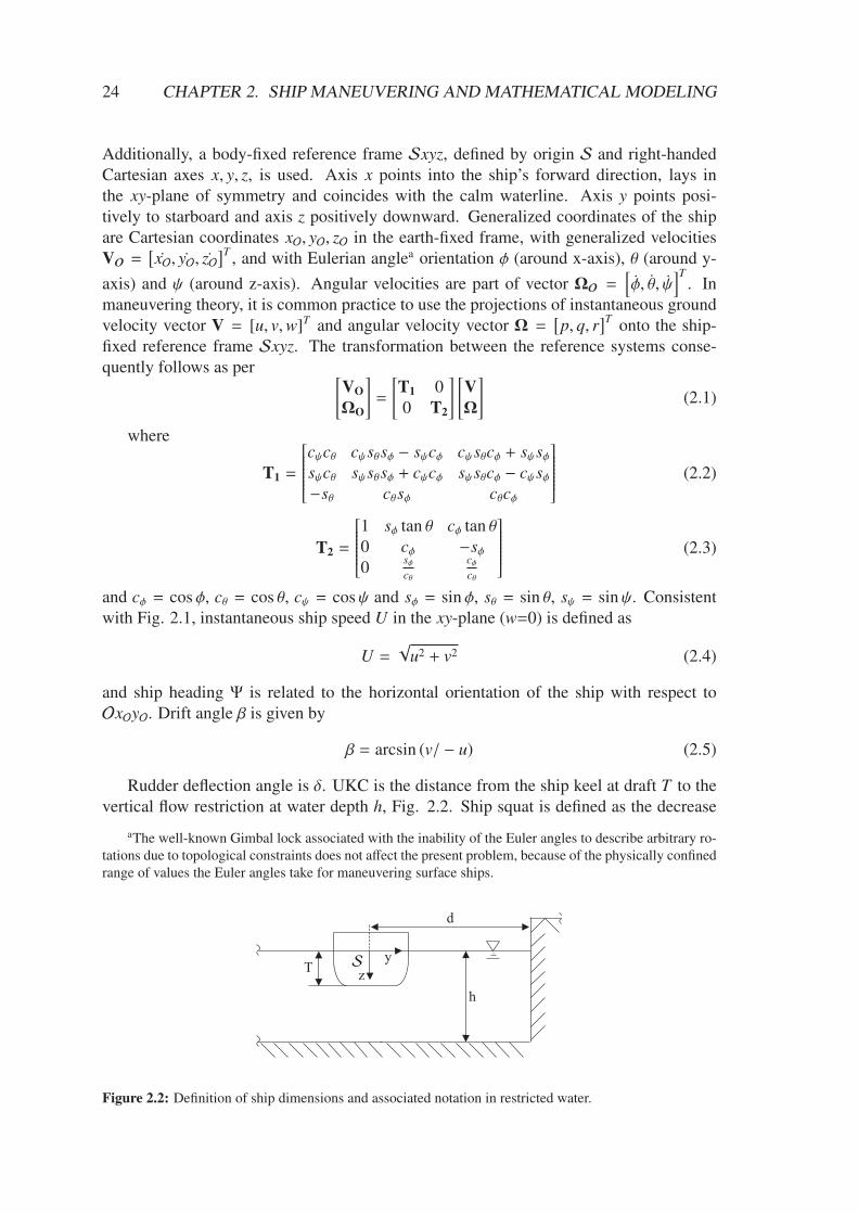
Rudder deflection angle is δ. UKC is the distance from the ship keel at draft T to thevertical flow restriction at water depth h, Fig. 2.2. Ship squat is defined as the decrease
aThe well-known Gimbal lock associated with the inability of the Euler angles to describe arbitrary ro-tations due to topological constraints does not affect the present problem, because of the physically confinedrange of values the Euler angles take for maneuvering surface ships.
z
yT
h
d
S
Figure 2.2: Definition of ship dimensions and associated notation in restricted water.
2.2. MANEUVERABILITY ASSESSMENT 25
of UKC in response to pressure variations along the ship hull underway, which cause theship to adjust her dynamic floating position in terms of a vertical translation (sinkage)and a rotational displacement in pitch mode of motion (trim), accompanied by a changeof the ambient free water surface level. The six-DoF hydrodynamic forces and momentsare denoted by X,Y,Z,K,M,N, Fig. 2.1. In straight ahead motion, ship resistance RT
equals the negative longitudinal hydrodynamic force X. Following common practice inship hydrodynamic analysis, results are presented in nondimensional form, where appro-priate. Nondimensional quantities are furnished with a prime, e.g. u′. Basic quantitiesfor nondimensionalization, if not stated otherwise, are water density ρ, ship speed U, andship length between perpendiculars L. For a generalized force component F it follows
F′ =F
0.5ρU2L2(2.6)
and for a generalized moment M with L as the characteristic length
M′ =M
0.5ρU2L3(2.7)
Rigid body velocities are made nondimensional as per
u′ =u
U; v′ =
v
U; r′ =
rL
U(2.8)
Further, propeller advance number J is introduced as per
J =Up
nDp(2.9)
where Up is propeller inflow velocity, see Eq. (2.49) , n propeller rate of revolution andDp propeller diameter. For ease of comparison with relevant references, therein estab-lished notation for particular expressions is adopted. This tangibly affects the notation forhydrodynamic forces, moments and rigid body velocities, i.e.
F2 ≡ Y,M3 ≡ N,V1 ≡ u,V2 ≡ v,Ω3 ≡ r
The established notation of Imlay (1961) denotes entries of the added mass tensor ai j asgiven in Newman (1978), see Eq. (2.25), by variables of hydrodynamic forces carryingindices of respective rigid body accelerations or velocities, e.g. a11 ≡ Xu, a22 ≡ Yv.
2.2 Maneuverability assessment
Ship maneuverability concerns dynamic response characteristics of ships to commandedchanges in direction of travel or speed through theur control surfaces, Newman (1966).Conventional control surfaces are rudders, propellers and fins. Bow and stern thrusters,as well as azimuthal pod-driven thrusters represent unconventional maneuvering devices.Maneuverability requirements refer to course, lane, or speed changing and keeping, aswell as to positioning. Maneuverability is rated based on the costs employed to meet theserequirements, e.g. the time to complete a maneuver, applied control effort or change of
26 CHAPTER 2. SHIP MANEUVERING AND MATHEMATICAL MODELING
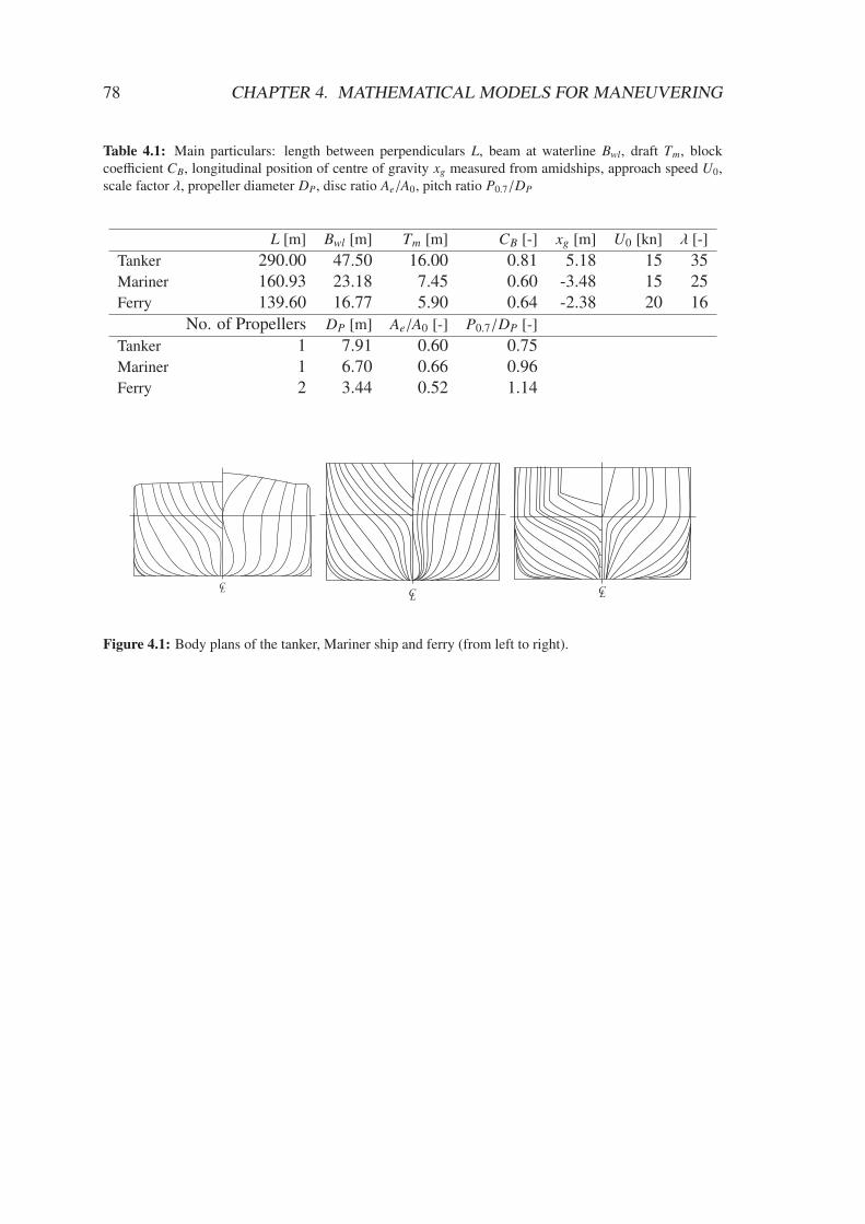
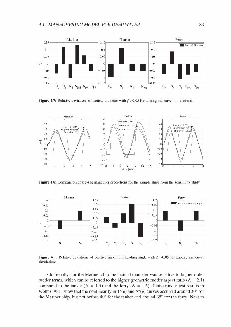
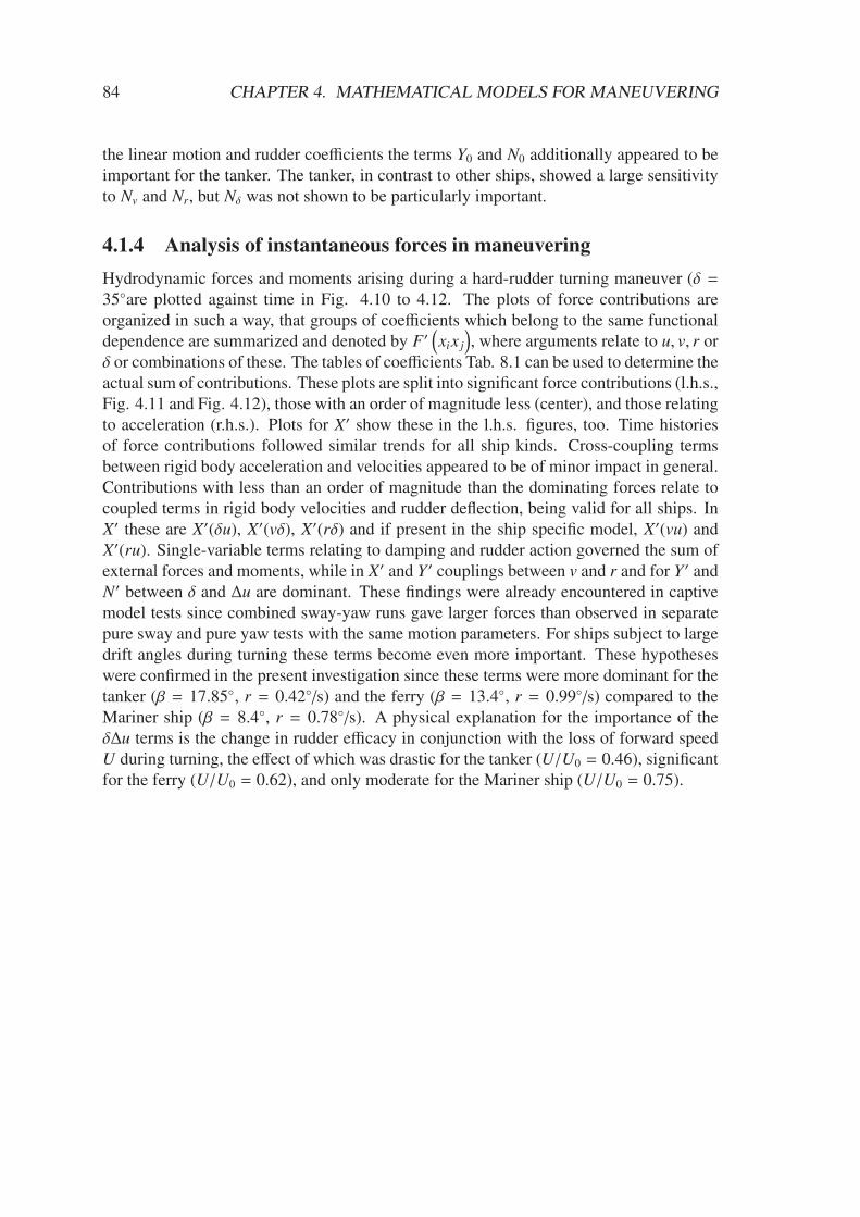
forward speed in response to maneuvering. Conventionally, these properties are checkedin sea trials with appropriate standard maneuvers. Associated guidelines and recommen-dations are issued by IMO (2002) and the maneuvering trial code of ITTC (1975). IMO’scriteria are non-binding, but the display of a poster on-board ships informing about gen-eral maneuvering properties is mandatory, IMO (1987). Sea trials represent the real sys-tem behavior free of scale effects or model assumptions, which are encountered in modelexperiments and simulation-based predictions. On other hand, environmental conditionslike winds, waves or currents impair the assessment of calm water maneuverability. Seatrials are also infeasible in the early stage of new ship designs in absence of sister ships,which emphasizes the need for alternative prediction methods. A host of standard ma-neuvers is available to study maneuverability. For the particular purpose of validationstudies for benchmarking of different prediction methods turning and zig-zag maneuvershave been established in the hydrodynamic community. Hard-rudder turning maneuversinvolve large-amplitude motions in sway and yaw, including excitations of nonlinear ef-fects , while zig-zag maneuvers offer valuable insight into the flow when control surfacesare dynamically varied in sign. The experimental analysis of maneuverability in shallowwater through maneuvering trials is impaired, because it is hard to find a test region withthe desired uniform water depth. According to the Permanent International Associationof Navigation Congresses (PIANC, 1992) extreme shallow water condition is present forwater depth to draft ratio h/T ≤ 1.2, Fig. 2.2. If UKC is in the order of anticipatedsquat for practically relevant forward speeds, ship operation has inevitably to be adaptedto prevent grounding. In laterally restricted waters, ship-induced wave loads on banksinfluence the choice of appropriate forward speeds. Apart from these special problems, inany restricted water, increasing hydrodynamic forces in all modes of motion are causativeto the increased response time to commanded changes in horizontal motion, as will beaddressed further down the line. Typical forward speeds of sea-going vessels with draftsin the order of 7 m (e.g. Feeders) to 20 m (e.g. Very Large Crude Carriers) lay between6 and 10 kts in presence of UKC of 20% of ship draft. These operational facts will beshown to affect the mathematical modeling of maneuvering in confined waters, too.
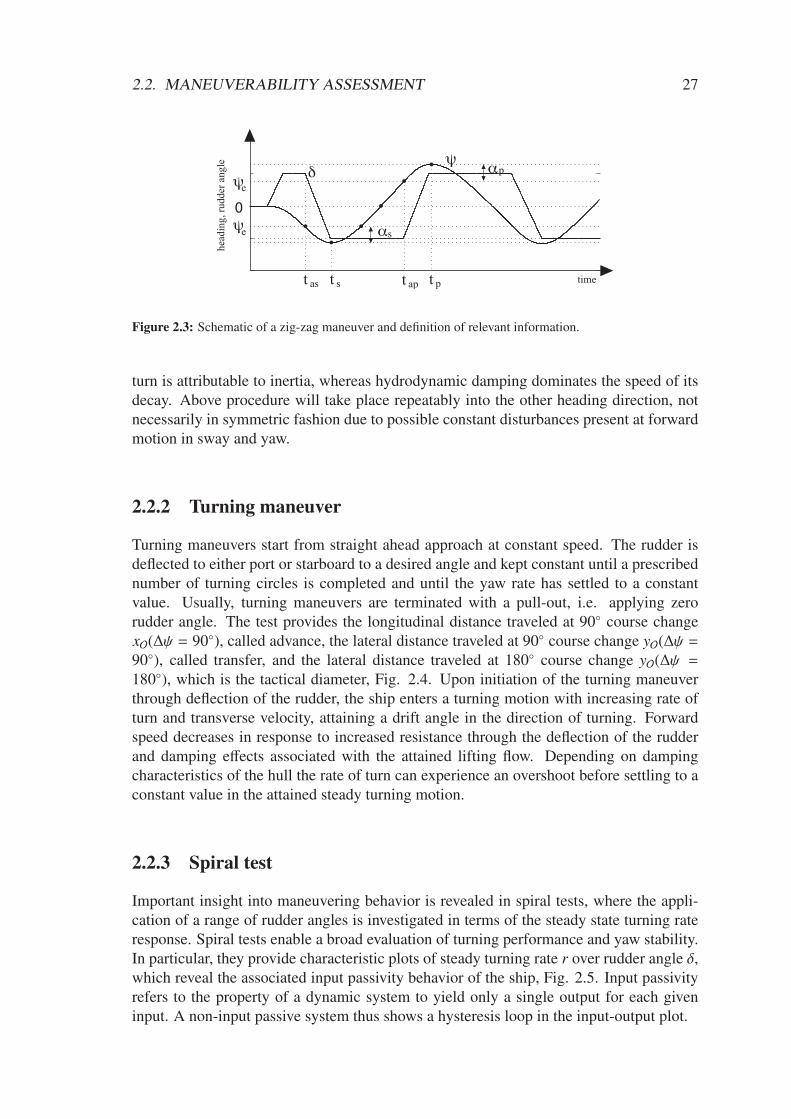
2.2.1 Zig-zag maneuver
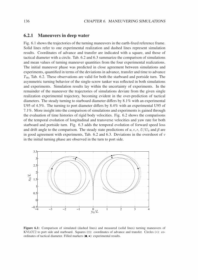
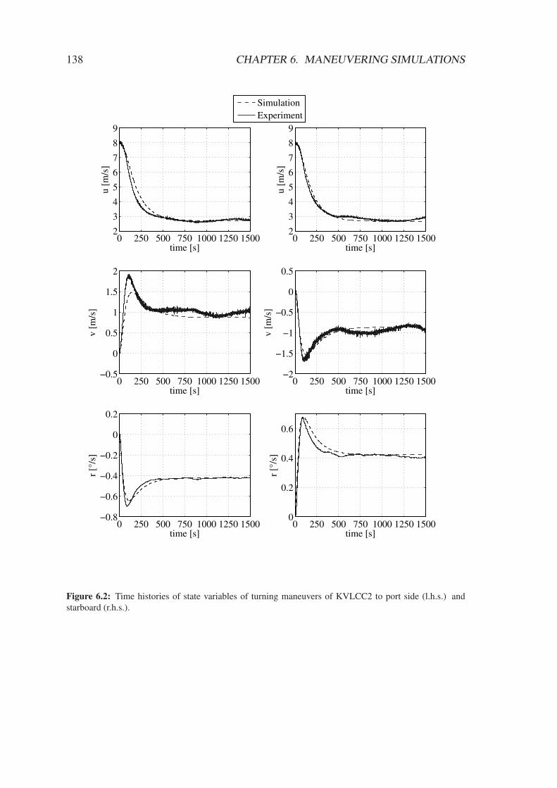
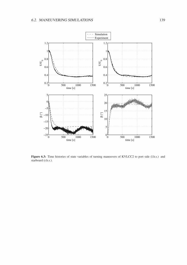
Zig-zag maneuvers start from straight ahead approach at constant speed. The rudder isdeflected to a desired angle. Typical values are 10, 20 or 35. Upon the desired changeof heading ∆Ψe counter-rudder is applied until the same course change ∆Ψe with respectto the initial course is reached in the opposite direction, Fig. 2.3. Typical values are 10
or 20. This procedure is repeated for an appropriate number of runs. The test gives ini-tial turning time tas, yaw checking time ts, overshoot angles to starboard αs and port sideαp. Upon initiation of the maneuver through deflection of the rudder, the ship enters aturning motion with increasing rate of turn and transverse velocity, attaining a drift anglein the direction of turning. Forward speed decreases in response to increased resistancethrough the deflection of the rudder and damping effects associated with the attained lift-ing flow. Upon application of counter-rudder, the rate of turn reaches its maximum andis decreased thereafter, still turning the ship into the same direction, until the rate of turnbecomes zero and the change in actual heading reaches its maximum. The difference toprescribed change of heading ∆Ψe is the overshoot angle. The gradual decrease in rate of
2.2. MANEUVERABILITY ASSESSMENT 27
δψ
0
ψ
ψ
t
α
as
e
e
t s
s
time
hea
din
g, ru
dder
angle
αp
t p t ap
Figure 2.3: Schematic of a zig-zag maneuver and definition of relevant information.
turn is attributable to inertia, whereas hydrodynamic damping dominates the speed of itsdecay. Above procedure will take place repeatably into the other heading direction, notnecessarily in symmetric fashion due to possible constant disturbances present at forwardmotion in sway and yaw.
2.2.2 Turning maneuver
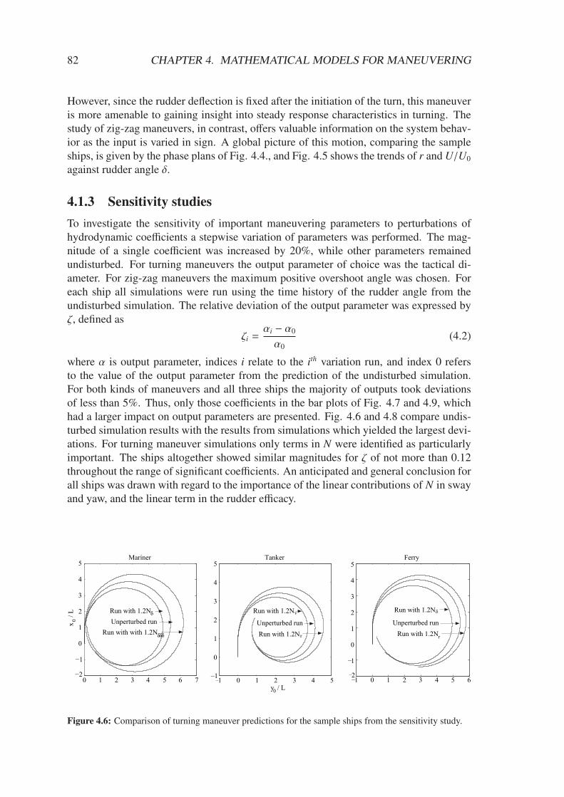
Turning maneuvers start from straight ahead approach at constant speed. The rudder isdeflected to either port or starboard to a desired angle and kept constant until a prescribednumber of turning circles is completed and until the yaw rate has settled to a constantvalue. Usually, turning maneuvers are terminated with a pull-out, i.e. applying zerorudder angle. The test provides the longitudinal distance traveled at 90 course changexO(∆ψ = 90), called advance, the lateral distance traveled at 90 course change yO(∆ψ =90), called transfer, and the lateral distance traveled at 180 course change yO(∆ψ =180), which is the tactical diameter, Fig. 2.4. Upon initiation of the turning maneuverthrough deflection of the rudder, the ship enters a turning motion with increasing rate ofturn and transverse velocity, attaining a drift angle in the direction of turning. Forwardspeed decreases in response to increased resistance through the deflection of the rudderand damping effects associated with the attained lifting flow. Depending on dampingcharacteristics of the hull the rate of turn can experience an overshoot before settling to aconstant value in the attained steady turning motion.
2.2.3 Spiral test
Important insight into maneuvering behavior is revealed in spiral tests, where the appli-cation of a range of rudder angles is investigated in terms of the steady state turning rateresponse. Spiral tests enable a broad evaluation of turning performance and yaw stability.In particular, they provide characteristic plots of steady turning rate r over rudder angle δ,which reveal the associated input passivity behavior of the ship, Fig. 2.5. Input passivityrefers to the property of a dynamic system to yield only a single output for each giveninput. A non-input passive system thus shows a hysteresis loop in the input-output plot.
28 CHAPTER 2. SHIP MANEUVERING AND MATHEMATICAL MODELING
y0(ψ=180°)y
0(ψ=90°)
x0(ψ=90°)
x0(δ=0°)
transfer tactical diameter
rudder execute
advance
Figure 2.4: Schematic of a turning maneuver and definition of relevant information.
−40 −30 −20 −10 0 10 20 30 40−1.5
−1
−0.5
0
0.5
1
1.5
δ [°]
rʹ
Figure 2.5: Spiral test results showing r against δ for a ship with input passivity (squares) and a ship withoutinput passivity (circles).
2.3 Maneuvering prediction
For simulation-based predictions and analyses of maneuvering a mathematical systemdescription is required. In developing a mathematical framework for maneuvering pre-diction it is assumed that ship shape, mass and mass distribution do not change in time.Consistent with this notion classic rigid body dynamics apply. The inertial response char-acteristics of ships are available from mechanics, while the sum of external forces andmoments is unknown. Formulations of hydrodynamic forces embracing all known flowphenomena, amenable to solution within short time, are not available. Difficulties in mod-eling hydrodynamic forces for maneuvering ships are related to the influence of viscosity
2.3. MANEUVERING PREDICTION 29
and ship-induced free surface disturbances. The constitution of a model structure dependson the application domain. Compared to the simulation of arbitrary ship motions involv-ing different engine settings, reduction in complexity and parameter identification effortare possible for the prediction of rudder maneuvers for a given engine operational con-dition. A mathematical description for inertial response characteristics is obtained fromNewtonian mechanics. The conservation of momentum is postulated by Newton’s SecondLaw:
F = md
dt
(
VO +ΩO × rg
)
(2.10)
where F = [X,Y,Z]T is external force vector and t is time. Distances to the center of
gravity (CoG) in the ship-fixed system are given by rg =[
xg, yg, zg
]T. Eq. (2.10) is valid, if
Coriolis and centripetal effects due to the rotation of the earth are neglected. Conservationof moment of momentum H satisfies
M =d
dtH + rg × m
d
dt
(
VO +ΩO × rg
)
(2.11)
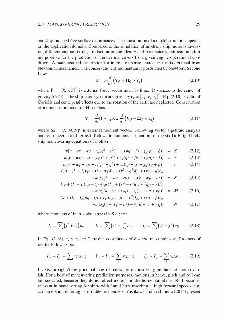
where M = [K,M,N]T is external moment vector. Following vector algebraic analysisand rearrangement of terms it follows in component notation for the six-DoF rigid bodyship maneuvering equations of motion
In Eq. (2.18), xi, yi, zi are Cartesian coordinates of discrete mass points mi Products ofinertia follow as per
Ixy = Iyx =∑
i
xiyimi; Ixz = Izx =∑
i
xizimi; Iyz = Izy =∑
i
yizimi (2.19)
If axis through S are principal axes of inertia, terms involving products of inertia van-ish. For a host of maneuvering prediction purposes, motions in heave, pitch and roll canbe neglected, because they do not affect motions in the horizontal plane. Roll becomesrelevant in maneuvering for ships with flared lines traveling at high forward speeds, e.g.containerships entering hard-rudder maneuvers. Yasukawa and Yoshimura (2014) present
30 CHAPTER 2. SHIP MANEUVERING AND MATHEMATICAL MODELING
a detailed investigation into the effect of roll motions on maneuvering. Operational con-ditions in shallow water do usually not excite significant roll motions. However, in driftmotions at low UKC low-pressure fields can be generated on the leeward side in the bilgeregion. The particular role of heave and pitch in the modeling of maneuvering in shallowwater is central to Chapter 2.5. The transverse CoG for port-starboard symmetric shipslays on the centerline, hence yg = 0. Under these assumptions, the equations of motionfor conventional surface ships can be studied in the horizontal plane comprising surge,sway and yaw
m(
u − vr − xgr2)
= X (2.20)
m(
v + ur + xgr)
= Y (2.21)
Izr + mxg (v + ur) = N (2.22)
2.4 Hydrodynamic forces and moments
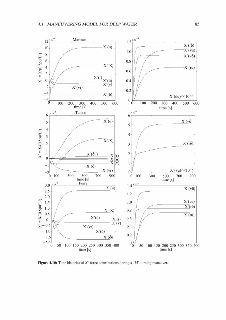
Having obtained a mathematical formulation of the inertial response characteristics of ma-neuvering surface vessels, the solution of the maneuvering equations requires knowledgeof hydrodynamic forces on the r.h.s. of Eq. (2.20-2.22). Discussions of modeling hy-drodynamic forces start with the unrestricted flow condition. Ship maneuvering involveslarge-amplitude motions in sway and yaw, which give rise to free surface disturbances andvorticity shed from the ship hull. These effects impair the formulation of a holistic theory,which would enable for a solution in practically reasonable time. There are theoretical andexperimental grounds to assume that in a given fluid, hydrodynamic forces on maneuver-ing ships depend on the shape of the hull, rigid body kinematics, control surface inputand external disturbances. Following the principle of divide and conquer, a pragmaticmodeling approach emerged in the hydrodynamic community to express the forces fol-lowing a decomposition of force effects. Decompositions have been established based onfundamental concepts of fluid dynamics. Predominately, this resulted in mathematical for-mulations for hydrodynamic forces in terms of coefficients, which represent ship-specifichydrodynamic properties, acting on state and control surface variables within the frame-work of coupled nonlinear differential equations of motion. The efforts associated withthe formulation and parameter identification of such motivated models are circumventedby transient numerical computations with field methods, which offer fine resolution of theflow around maneuvering ships in space and time by solving the Navier-Stokes equations.Hydrodynamic forces are available from the numerical solution itself, demonstrated byel Moctar et al. (2014) and Carrica et al. (2013) for standard rudder maneuvers in deepwater. Transient numerical computations were shown to be very expensive and requiredthe presence of High Performance Computing (HPC) environments. The time required toobtain the prediction of a standard rudder maneuver at a given operational condition is inthe order of several days to weeks, el Moctar et al. (2014), and rendered impractical forparametric investigations. When attempting to arrive at simplified models, the problememerges of identifying above introduced ship-specific hydrodynamic coefficients. On onehand, so-called modular models have been established. Force effects are formulated forthe ship hull and control surfaces separately; and these modules may include decomposi-tions themselves. Modular models are advocated by the possibility to study variations in
2.4. HYDRODYNAMIC FORCES AND MOMENTS 31
single system components in an economic way, as terms unaffected by variations remainconstant. On other hand, so-called global models seek to find hydrodynamic propertiesby integral evaluation of forces on the ship including all system contributions of the fullyequipped ship. Often, they are established to cover only a limited perturbation range froma given approach condition to a maneuver. Within the notion of global models interactionsbetween the hull and control surfaces are included in the coefficients without additionalmodeling or identification effort. Global models thus appeal to investigations of standardrudder maneuvers at a given approach speed. Parameter identification of global modelsis a pure exercise of model experiments and regression analysis. Disadvantages associ-ated with modular models are the need for further modeling assumptions with regard tointeractions of system components. Prior to the formulation of a model for the presentpurpose of demonstrating simulation-based maneuvering predictions in deep and shallowwater, a summary is given of the concept of the decomposition of forces, which facilitatesthe comprehension of force effects in maneuvering.
2.4.1 Decomposition of force effects
Hydrodynamic forces are seen as a superposition of various force effects. A typical de-composition for a generalized force and moment component F was discussed by Sharma(1982) and takes the form
F = FI + FL + FCF + FR + FP (2.23)
where index I stands for ideal flow, L for lift, CF for cross-flow, R is referred rudders, andP to propellers. Forces FI relate to inertial forces as present in inviscid and vorticity-freeflow. Lift forces FL emerge from the introduction of vorticity and associated effects fromthe general theory of wings including lift and induced drag in oblique flows. Cross-flowforces FCF include pressure and friction resistance to the ship hull in drift and yaw andcombined drift-yaw motion. Inertial force contributions are significant in accelerationphases, and usually an order of magnitude less than the dominating lift and cross-flowforces. Forces induced by propeller action mainly concern the longitudinal mode of mo-tion, as propeller thrust seeks to cancel ship resistance to forward motion. However, inmaneuvering propeller blades in oblique flow can generate lateral forces which typicallyare an order of magnitude less than thrust, but affect the sway and yaw modes of motion.Above decomposition motivated the formulation of a modular mathematical model forarbitrary rudder-engine maneuvers within the four-quadrants of ship operation, where-upon the different force contributions are expressed as functions only to the four anglesaddressing the states of engine operation (forward/reverse) and direction of motion (for-ward/backward), Oltmann and Sharma (1979):
β; γ = arctan(rL
2u
)
; δe = δ + βR; ǫp = arctan
(Cp
Up
)
(2.24)
In Eq. (2.24) γ is yaw angle , δe is effective rudder angle taking into account the rudderdrift angle βR, see Eq. (2.42), ǫp propeller advance angle, Cp = 0.7πnDp, with n propellerrevolutions and Dp propeller diameter.
32 CHAPTER 2. SHIP MANEUVERING AND MATHEMATICAL MODELING
Ideal flow effects
A quintessential finding from potential flow theory is that forces acting on arbitrarilyshaped bodies moving arbitrarily in an unbounded, ideal fluid are related to entries of thehydrodynamic added mass tensor, Newman (1978)
ai j = ρ
∫
S
φi
∂φ j
∂ndS . (2.25)
where S is body surface and n its normal vector. Dependencies between the added masstensor and rigid body kinematics are established through Kirchoff’s (1869) equations forfluid kinetic energy. Upon the introduction of symmetry properties of the ship hull withrespect to the waterline and midship plane, Sharma (1982) formulated the ideal flow forceeffects in component notation as per
XI = Xuu − Yvrv − Yrr2 (2.26)
YI = Yvv − Xuru − Yrr (2.27)
NI = Nrr + (Yv − Xu) uv + Nv (v + ur) (2.28)
Eq. (2.28) includes the well-known broaching moment term (Yv − Xu) uv, which came tobe called Munk moment, Munk (1924).
Lifting flow effects
Lifting flow effects are seen as potential flow effects under consideration of vortices of abody in oblique flow. In this concept, a ship is considered as a wing of aspect ratio 2T/L.Classic wing theories of Prandtl and Tietjens (1957) were applied to a ship by Sharma(1982). Lifting forces are formulated as functions of aspect ratio, drift angle, stagnationpressure and effective inflow at the transom of the ship, and moments are found frommultiplication with appropriate lever arms. The respective forms of XL, YL and NL read
XL =ρ
2LT
u(
−√c1v +√
c2r0.5L sgn u)2
√u2 + v2 + 0.5L2
[
1 − d1v2 + d2r20.5L2
u2 + v2 + r2 + 0.5L2
]
(2.29)
YL =ρ
2LT
[ −c1u2v√u2 + v2
(
1 +d1v2
u2 + v2
)
+c2u |u| r0.5L√u2 + v2 + 0.5L2
(
1 +d2r20.5L2
u2 + v2 + 0.5L2
)]
(2.30)
NL =ρ
2L2T
[
e1u |u| v√u2 + v2
(
1 +d1v2
u2 + v2
)
− e2u2r0.5L√u2 + v2 + 0.5L2
(
1 +d2r20.5L2
u2 + v2 + 0.5L2
)]
(2.31)
where c1 is drift coefficient, c2 is yaw coefficient, di, i = 1, 2, are combined drift andyaw coefficients and ei, i = 1, 2, are lever arm coefficients for drift and yaw, respectively.Coefficients are found from drift, yaw and combined drift and yaw experiments, Sharma(1982). Bollay (1936) studied the flow past wings of low-aspect ratio in the nonlinearlifting theory of rectangular plates. A fundamental conclusion was that bound vorticeswere assumed to be constant along the wing span, elliptically distributed along the chordand leave the tip of the chord as a horse-shoe vortex trailing at an angle half of the angleof attack. Inoue (1969) presents an application to ship flows.
2.4. HYDRODYNAMIC FORCES AND MOMENTS 33
−1 −0.8 −0.6 −0.4 −0.2 0 0.2 0.4 0.6 0.8 10
1
2
3
4
5
c D
x/l
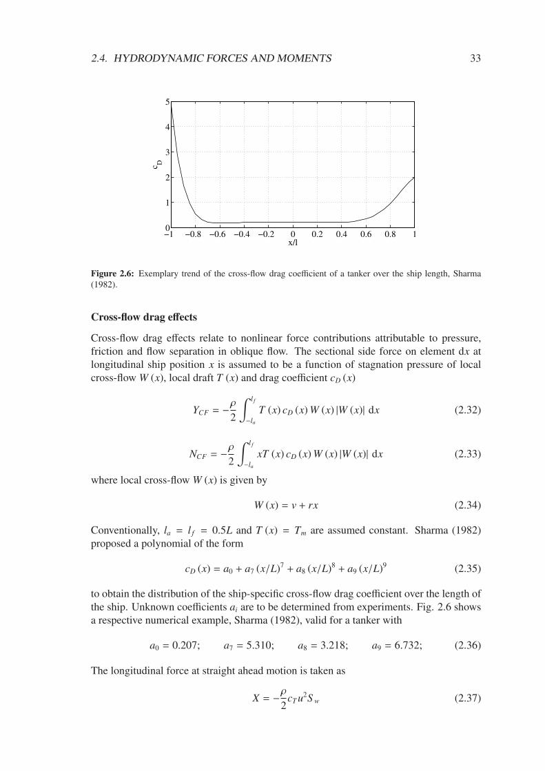
Figure 2.6: Exemplary trend of the cross-flow drag coefficient of a tanker over the ship length, Sharma(1982).
Cross-flow drag effects
Cross-flow drag effects relate to nonlinear force contributions attributable to pressure,friction and flow separation in oblique flow. The sectional side force on element dx atlongitudinal ship position x is assumed to be a function of stagnation pressure of localcross-flow W (x), local draft T (x) and drag coefficient cD (x)
YCF = −ρ
2
∫ l f
−la
T (x) cD (x) W (x) |W (x)| dx (2.32)
NCF = −ρ
2
∫ l f
−la
xT (x) cD (x) W (x) |W (x)| dx (2.33)
where local cross-flow W (x) is given by
W (x) = v + rx (2.34)
Conventionally, la = l f = 0.5L and T (x) = Tm are assumed constant. Sharma (1982)proposed a polynomial of the form
cD (x) = a0 + a7 (x/L)7+ a8 (x/L)8
+ a9 (x/L)9 (2.35)
to obtain the distribution of the ship-specific cross-flow drag coefficient over the length ofthe ship. Unknown coefficients ai are to be determined from experiments. Fig. 2.6 showsa respective numerical example, Sharma (1982), valid for a tanker with
The longitudinal force at straight ahead motion is taken as
X = −ρ2
cT u2S w (2.37)
34 CHAPTER 2. SHIP MANEUVERING AND MATHEMATICAL MODELING
where S w is wetted surface area, and relies on conventional drag coefficients from the
ITTC 1978 method, ITTC (1999)
cT = (1 + k) cF (Re) + cW (Fn) (2.38)
where cF is determined from the plate friction correlation line, cW is wave resistance
coefficient and k form factor, found from experiments. Reynolds number is Re and Froude
number Fn, see Chapter 4. Hooft (1994) covers theoretical considerations on the cross-flow drag concept.
Rudder forces
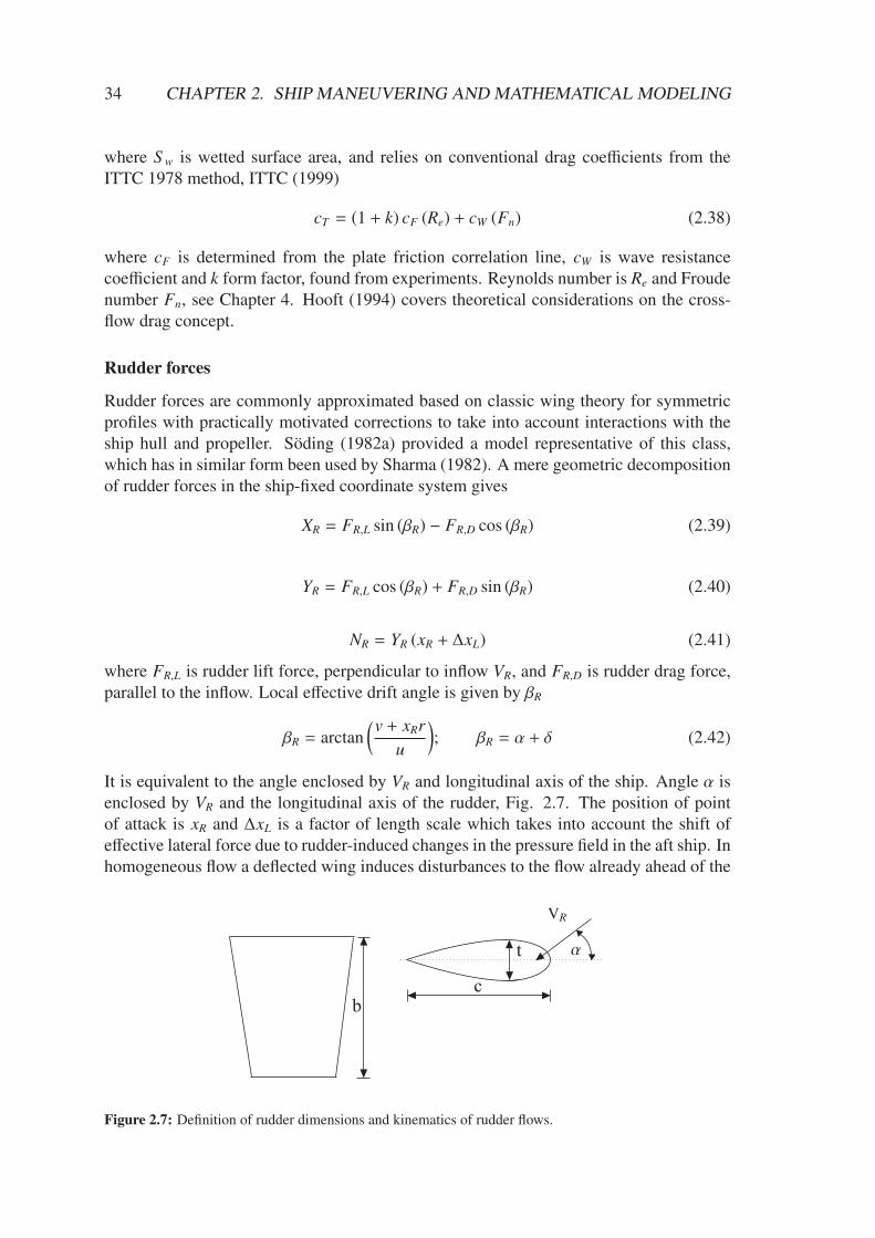
Rudder forces are commonly approximated based on classic wing theory for symmetricprofiles with practically motivated corrections to take into account interactions with theship hull and propeller. Söding (1982a) provided a model representative of this class,which has in similar form been used by Sharma (1982). A mere geometric decompositionof rudder forces in the ship-fixed coordinate system gives
XR = FR,L sin (βR) − FR,D cos (βR) (2.39)
YR = FR,L cos (βR) + FR,D sin (βR) (2.40)
NR = YR (xR + ∆xL) (2.41)
where FR,L is rudder lift force, perpendicular to inflow VR, and FR,D is rudder drag force,parallel to the inflow. Local effective drift angle is given by βR
βR = arctan(v + xRr
u
)
; βR = α + δ (2.42)
It is equivalent to the angle enclosed by VR and longitudinal axis of the ship. Angle α isenclosed by VR and the longitudinal axis of the rudder, Fig. 2.7. The position of pointof attack is xR and ∆xL is a factor of length scale which takes into account the shift ofeffective lateral force due to rudder-induced changes in the pressure field in the aft ship. Inhomogeneous flow a deflected wing induces disturbances to the flow already ahead of the
t
cb
VR
α
Figure 2.7: Definition of rudder dimensions and kinematics of rudder flows.
2.4. HYDRODYNAMIC FORCES AND MOMENTS 35
tip upstream. This effect is intensified through the presence of the hull, which impedes the
balance of the mentioned disturbances as encountered in free inflow. A pressure difference
between port and starboard results, increasing the total rudder-induced force on the hulland rudder and shifting its effective point of attack in positive x-direction. At the sametime, the presence of the hull affects the effective inflow to the rudder. Consistent withclassic wing theory, FR,L and FR,D are found from
FR,L = 0.5ρcR,LV2RAR; FR,D = 0.5ρcR,DV2
RAR (2.43)
where AR is rudder surface area, cR,L is rudder lift coefficient and cR,D is rudder dragcoefficient, approximated by
cR,L =2πΛ (Λ + 1)
(Λ + 2)2sinα + cQ sinα |sinα| cosα (2.44)
where Λ = b2/AR is geometric rudder aspect ratio and cQ induced-drag coefficient inlateral rudder inflow. For drag coefficient cR,D it follows
cR,D =1πΛ
(
2πΛ (Λ + 1)
(Λ + 2)2sinα
)2
+ cQ
∣∣∣sin3 α
∣∣∣ + 2cF (2.45)
Usually, cR,L, cQ, and cR,D are found from model tests and are available in tables of dif-ferent profiles and Reynolds numbers, Abbott and Doenhoff (1959), Whicker and Fehlner(1958), Thieme (1992). The propeller slipstream affects the rudder inflow as propellerracing increases the effective wash on the rudder surface. Söding (1982a) suggests to takethe local velocity of a location far behind the propeller as
VR = u (1 − w)√
1 + cT H (2.46)
where cT H = 8KT/(J2π) is thrust load coefficient and w is nominal wake fraction numberand thrust coefficient KT defined in Eq. (2.47). Similar approximations for finite positionsbehind the propeller are found in Sharma (1982) and Gutsche (1952). In Söding (1982a,1982b) the particular arrangement of the rudder in the aft ship, including the clearanceto the hull or the free surface, factor into the formulations of rudder forces in terms ofcoefficients, which in the reference are suggested to be available from BEM computationsusing lifting line theory. Theoretical treatise of lifting line theory is given in Newman(1978). Oltmann and Sharma (1979) demonstrate the application of such rudder forcemodels to a maneuvering model for simulation of arbitrary engine-rudder maneuvers.A representative example for the use of semi-empirical hull-propeller-rudder interactioncoefficients in maneuvering models is given in Yasukawa and Yoshimura (2015). The flowaround rudders in homogeneous flow, and in the case of fully-appended ships involvinghull-propeller-rudder interactions were shown to be accurately predictable with CFD, elMoctar (2001b).
Propeller forces
Propeller forces for maneuvering models can be obtained from open-water propeller per-formance curves derived for different operational settings, and wake and thrust deduction
36 CHAPTER 2. SHIP MANEUVERING AND MATHEMATICAL MODELING
0 0.1 0.2 0.3 0.4 0.5 0.6 0.7 0.80
0.1
0.2
0.3
0.4
0.5
0.6
0.7
J
KT,
10
KQ
, η
10KQ
KT
η
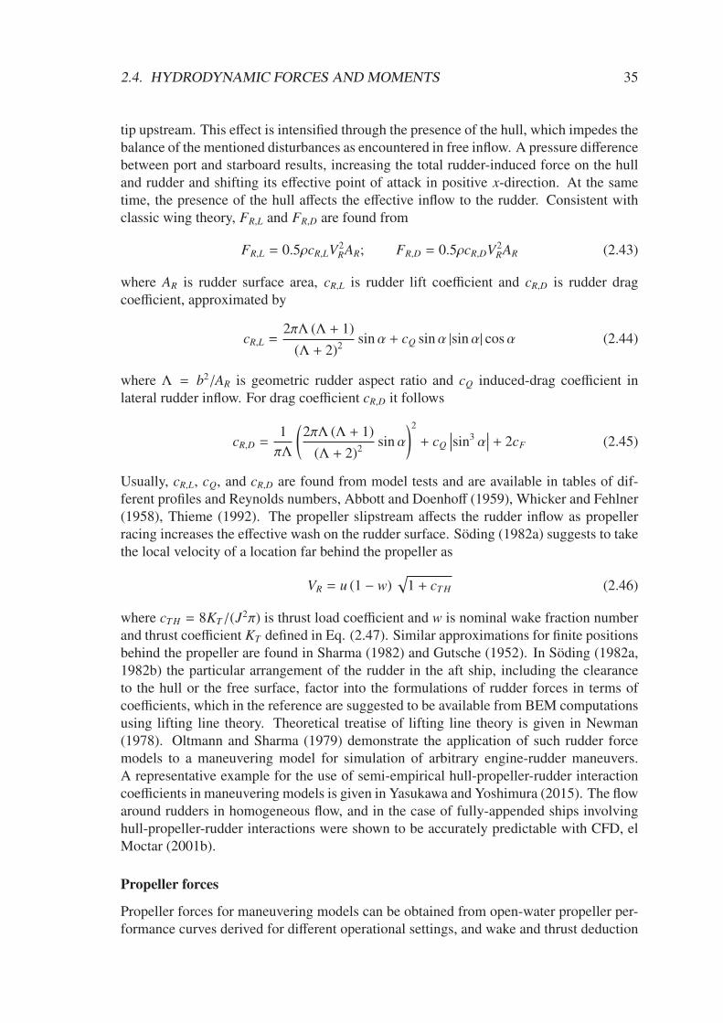
Figure 2.8: Open water propeller performance diagramme.
factors found from propulsion tests, Sharma (1982). The results of such tests are thrust
coefficient KT and torque coefficient KQ, Fig. 2.8
KT =T
ρn2D4p
(2.47)
KQ =Q
ρn2D5p
(2.48)
which are functions of J, using by local inflow speed
Up = u (1 − w) (2.49)
In the longitudinal mode of motion, the propeller force contribution would enter the r.h.s.
of the maneuvering equations as
Xp = T (1 − t) (2.50)
where t is thrust deduction factor. Thrust and torque affect maneuvering in terms of the
effective wash on the rudder surface. In oblique flows the propeller generates lateral
forces which can significantly contribute to the balance of forces and moments. Then, the
effective angle of attack αe varies as a function of the blade’s circumferential position θ.
This gives rise to transverse forces on the propeller shaft, a transverse shift of the center
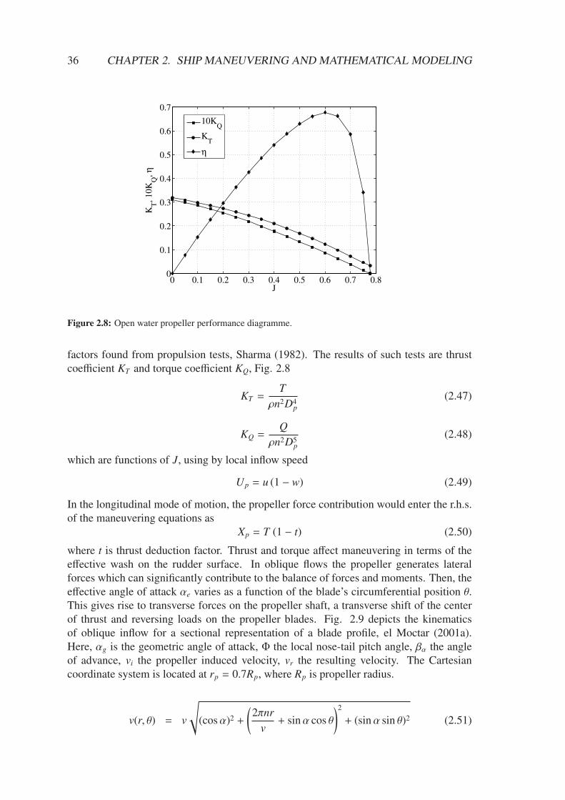
of thrust and reversing loads on the propeller blades. Fig. 2.9 depicts the kinematics
of oblique inflow for a sectional representation of a blade profile, el Moctar (2001a).
Here, αg is the geometric angle of attack, Φ the local nose-tail pitch angle, βα the angleof advance, vi the propeller induced velocity, vr the resulting velocity. The Cartesiancoordinate system is located at rp = 0.7Rp, where Rp is propeller radius.
v(r, θ) = v
√
(cosα)2 +
(
2πnr
v+ sinα cos θ
)2
+ (sinα sin θ)2 (2.51)
2.4. HYDRODYNAMIC FORCES AND MOMENTS 37
2πnr
xp
yp
yp
zpω
βαΦ
αgαe
vr vi
vα
v
v
θ = 0
θ = 90
α
α
Figure 2.9: Kinematics of oblique propeller inflow, reproduced from el Moctar and Bertram (2000).
βα = tan−1
( v cosα
πnr + v sinα cos θ
)
(2.52)
The x-axis points into the ship’s forward direction, the y-axis points to portside and thez-axis points upwards. The sign of the angle of inflow α is positive in Fig. 2.9. In acylindrical coordinate system fixed to the propeller axis, Eq. (2.51) follows for the inflowvelocity vα. If the blades runs against the oblique flow, propeller forces increase withthe increase of angle of attack and velocity. If the blade runs with the oblique flow inthe other half of the rotation, the opposite effect takes place, but forces decrease by asmaller magnitude. The resulting mean thrust and torque are larger than in homogeneousinflow and functions of J and α; and a transverse force perpendicular to the propeller axisarises. The point of attack of mean thrust moves towards the side the blade runs against,which induces a moment about the vertical axis in Sxyz. The distance of this shift alsoincreases with J and α. El Moctar and Bertram (2000) showed from numerical analysisthat the mean lateral force generated by horizontal oblique inflow can be 18% of propellerthrust, and the shift of the thrust point of attack can be 10% of the propeller radius forJ = 0.7. In the numerical example the drift angle of the investigated tanker was β = 12.The presence of the hull diminishes this effect due to its flow-directing function to thepropeller. Maneuvering model tests or CFD computations which include the propellerconsider these effects in measuring or computing integral forces and moments on the hull.
Influence of engine dynamics
Hull forces are increased in maneuvering. Propeller torque increases to an upper thresh-old in response, determined by the engine characteristics, and decreases correspondinglythe propeller rate of revolution. The so-emerging interaction between hull, propeller andengine affects rudder forces. Engine dynamics are usually excluded in ordinary maneu-vering simulations which seek to compute general maneuvering properties from standardmaneuvers, but are an essential requirement for ship handling simulations. Related dis-cussions on the impact on maneuvering is provided in el Moctar and Cura-Hochbaum(2005) and el Moctar et al. (2014).
38 CHAPTER 2. SHIP MANEUVERING AND MATHEMATICAL MODELING
2.4.2 Multivariat polynomial models
The first consequent formulation of a global maneuvering model using multivariat alge-braic polynomials for an integral evaluation of forces and moments for the fully-equippedship in a given fluid is related to Abkowitz (1964). The starting point are Taylor-seriesexpansions in powers of the variables of a functional like
F = f(
x0, y0, ψ, u, v, r, u, v, r, δ, δ, δ)
(2.53)
The functional may be extended by propeller revolution n, or any other parameter con-sidered to affect F. This notion presumes continuous functions and derivatives for theconsidered range of operation. It follows
X(x) ≈ X(x0) +n∑
i=1
∂X(x)∂xi
∣∣∣∣∣x0
∆xi +12∂2X(x)
∂x2i
∣∣∣∣∣∣x0
∆x2i +
16∂3X(x)
∂x3i
∣∣∣∣∣∣x0
∆x3i + ...
(2.54)
Y(x) ≈ Y(x0) +n∑
i=1
∂Y(x)∂xi
∣∣∣∣∣x0
∆xi +12∂2Y(x)
∂x2i
∣∣∣∣∣∣x0
∆x2i +
16∂3Y(x)
∂x3i
∣∣∣∣∣∣x0
∆x3i + ...
(2.55)
N(x) ≈ N(x0) +n∑
i=1
∂N(x)∂xi
∣∣∣∣∣x0
∆xi +12∂2N(x)
∂x2i
∣∣∣∣∣∣x0
∆x2i +
16∂3N(x)
∂x3i
∣∣∣∣∣∣x0
∆x3i + ...
(2.56)
wherex =
[
x0, y0, ψ, u, v, r, u, v, r, δ, δ, δ]T
(2.57)
and the perturbation from the equilibrium state is ∆x = x − x0 = [∆x1,∆x2,∆x3, ...,∆xn]T .The established notation (Imlay, 1961) for the emerging partial derivatives is
Yv =∂Y
∂v
∣∣∣∣∣x=x0
,Yvv =12∂2Y
∂v2
∣∣∣∣∣∣x=x0
, · · · (2.58)
as an example for the derivative in Y with respect to v. For higher-order terms the index ispowers of v. The so-defined coefficients are called hydrodynamic derivatives. From a for-mal point of view, the emerging unknown coefficients do not represent derivatives, but theterminology has widely been adopted in the ship hydrodynamic community, (Sutulo andGuedes Soares, 2011). In the remainder, they will be called hydrodynamic coefficients.Above approach is valid for an equilibrium point from which the motion of interest de-parts. Often this is the straight ahead condition at a certain approach speed U0, with v, rand δ being zero. Assuming that the longitudinal hull force cancels the propeller thrust T ,no net force acts on the ship hull in this condition, X0 = T . The expansion results in a largenumber of unknown hydrodynamic coefficients. Initial assumptions to reduce the numberof parameters are that force and moment contributions related to rudder action solely de-pend on rudder deflection δ, rather than its temporal derivatives. Forces are also assumedto be independent of initial position x0, y0, and orientation ψ0. Further, if accelerationforces exclusively result from inertia properties not interacting with viscous effects, asdictated by potential flow theory, only linear terms have to be retained. In ship maneuversexhibiting large departures from the equilibrium state, nonlinearities are dominant raisingthe questions of which powers in the expansion are relevant. Following Abkowitz (1964)
2.4. HYDRODYNAMIC FORCES AND MOMENTS 39
it was sufficient to include the nonlinearity up to third order. A detailed discussion of
relevant powers in the expansion is governed by geometric properties in conjunction with
physical considerations treated separately for surge, sway and yaw. Hence, port-starboardsymmetry of ships suggests only to keep even powers of v, r and δ in X. Considering thatthese force contributions depend on angle of attack, itself influenced by forward velocityu, it follows that these forces vary with u. With these considerations, the nonlinear formof X reads
where ∆u = u −U0 is the perturbation from the approach speed. In deriving formulationsfor Y and N, the same arguments are invoked, considering that along with symmetryconsiderations, terms for v, r and δ are now odd functions. Additionally, if for zerorudder deflection the ship has a turning moment N0 and a side force Y0, these terms areconsidered as well as combinations with ∆u to account for their change with forwardspeed. Analogous forms of Y and N, correspondingly, under these assumptions read
Hydrodynamic coefficients are usually determined through model experiments. Here, twokinds of parameter identification methods are available. In direct parameter identificationcoefficients are found from systematic captive model tests and regression analysis of re-sulting force records. In indirect parameter identification, time histories of state variablesand inputs of free-running tests are processed with appropriate identification algorithms.For various coefficients, empirical formulas exist (Clarke et al., 1983), stemming frommodel tests and having limited use for ships and operational conditions outside of theframework of this investigation.
General objections
Fundamental objections associated with the presented approach were communicated ini-tially in conjunction with the advance of PMM experiments, which had their birth innaval hydrodynamics at David Taylor Model Basin (DTMB), Gertler (1959) and Good-man (1966). The summary mainly refers to Newman (1966) and SFB 98, Oltmann (1978).Abkowitz’s model assumes that hydrodynamic forces and moments are analytic functionsonly of instantaneous accelerations, velocities and displacements, i.e. that they remain in-dependent of the history of the hull-water interaction. A more exact model would consideralso the dependence of F on past motions by means of a convolution integral, as presentedby Cummins (1962). Physical phenomena giving rise to memory effects primarily dependon free surface disturbances and vorticity. The use of slow motion hydrodynamic coef-ficients is referred to the relatively long time, during which the dynamic response of aship to a commanded change in the direction of motion takes place. Identification of hy-drodynamic coefficients was predominately done via captive oscillatory model tests, and
40 CHAPTER 2. SHIP MANEUVERING AND MATHEMATICAL MODELING
frequency effects were also of concerns in model tests themselves. ITTC recommended
guidelines and procedures (2014) and reference therein treat this particular problem, see
also a study by Renilson (1986). The guidelines can generally not be transferred straight-forwardly to the shallow water case, because both free surface disturbances and vorticitychange, and it is anticipated that they are functions of oscillation frequency. Fundamentalobjections associated with the presented approach were communicated initially in con-junction with the advance of PMM experiments, which had their birth in naval hydro-dynamics at David Taylor Model Basin (DTMB), Gertler (1959) and Goodman (1966).The summary mainly refers to Newman (1966) and SFB 98, Oltmann (1978). Abkowitz’smodel assumes that hydrodynamic forces and moments are analytic functions only of in-stantaneous accelerations, velocities and displacements, i.e. that they remain independentof the history of the hull-water interaction. A more exact model would consider also thedependence of F on past motions by means of a convolution integral, as presented byCummins (1962). Physical phenomena giving rise to memory effects primarily depend onfree surface disturbances and vorticity. The use of slow motion hydrodynamic coefficientsis referred to the relatively long time, during which the dynamic response of a ship to acommanded change in the direction of motion takes place. Identification of hydrodynamiccoefficients was predominately done via captive oscillatory model tests, and frequency ef-fects were also of concerns in model tests themselves. ITTC recommended guidelinesand procedures (2014) and reference therein treat this particular problem, see also a studyby Renilson (1986). The guidelines can generally not be transferred straightforwardly tothe shallow water case, because both free surface disturbances and vorticity change, andit is anticipated that they are functions of oscillation frequency.
Model specific objections
The second major objection in Newman (1966) relates to the proposed Taylor-series ex-pansion wherein the side force is expressed as an odd function in cubic power of v, at-tributable to port-starboard symmetry. However, Newman (1966) remarks that both intheory and experiment for slender bodies with transverse symmetry in steady drift motionthe side force contribution associated with flow separation drag is of second-order of driftangle β:
Y ≈ A sin 2β + B sin β |sin β| (2.61)
≈ 2Aβ + Bβ |β| + O(
β3)
In Eq. (2.61) A and B are constant unknown coefficients. Emphasizing that force con-tributions associated with lifting-surface theory in an ideal fluid can be expressed withthe Taylor-series approach, Newman (1966) concludes that both second- and third-orderterms should appear in the side force and yaw moment of a nonlinear model. In thiscontext, special attention is drawn to extrapolation since separation drag is amenable toReynolds scaling rather than Froude similarity. However, the validity of these assump-tions remains questionable for bluff ships which exceed beam to length ratios of 0.15. Forsingle-screw ships model assumptions from symmetry considerations are controversial.Oltmann and Wolff (1979) argue that the mere introduction of constant side force andyaw moment terms Y0,N0 is too simple and consequent modifications to the model extendto the consideration of odd powers in the expansion for X and even powers in Y and N,
2.5. SHALLOW WATER EFFECTS ON MANEUVERING 41
respectively. Moreover, they also call for a modification of rudder coefficients towards
higher-order terms than O(
δ4)
, to more accurately capture flow separation at large rudderdeflections. The argumentation is challenged by scale effects involved in the extrapolationof the results from regression analysis performed at model scale to the dimensions of theship, since stall conditions are dependent on Reynolds number. Stall occurs at greaterangles with increasing Reynolds number. Oltmann and Wolff (1979) also plea for consid-ering cross-couplings between acceleration and velocities, and the nonlinear dependenceon accelerations, which is neglected in Abkowitz’s model. Other experimental investi-gations back the simplification, Strøm-Tejsen and Chislett (1966). Of additional concernis if the identified significance of the contributions in idealized captive model tests is en-countered in simulated free-running maneuvers and full-scale ship flows. Viallon et al.(2012) argue that neither polynomials of order higher than three, nor terms consideringacceleration-velocity coupling must be used in ship maneuvering. Sutulo and GuedesSoares (2011) address the issue of multicollinearity and over-parametrization in conjunc-tion with the use of both second-order modulus functions and third-order polynomialsto express damping forces. Experimental evidence contributing to the discussion is pre-sented in Kose (1982), who concluded with the recommendation for the use of algebraicpolynomials of order three. Multivariat polynomial models are readily applicable to theformulation of hull forces in a modular maneuvering model, too. A popular approachis to substitute the separate treatment of ideal, lifting and cross-flow effects by introduc-ing mulitivariat polynomials of the rigid body kinematic variables. For consideration ofa wide operational range of rigid body kinematic variables, models have been proposedusing Fourier series in terms of drift and yaw angle instead of polynomials of v and r, e.g.Gronarz (1997).
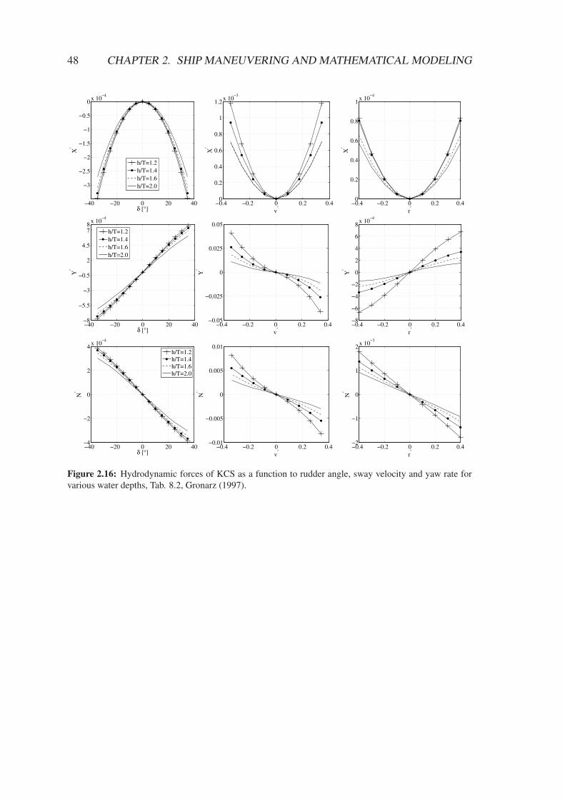
2.5 Shallow water effects on maneuvering
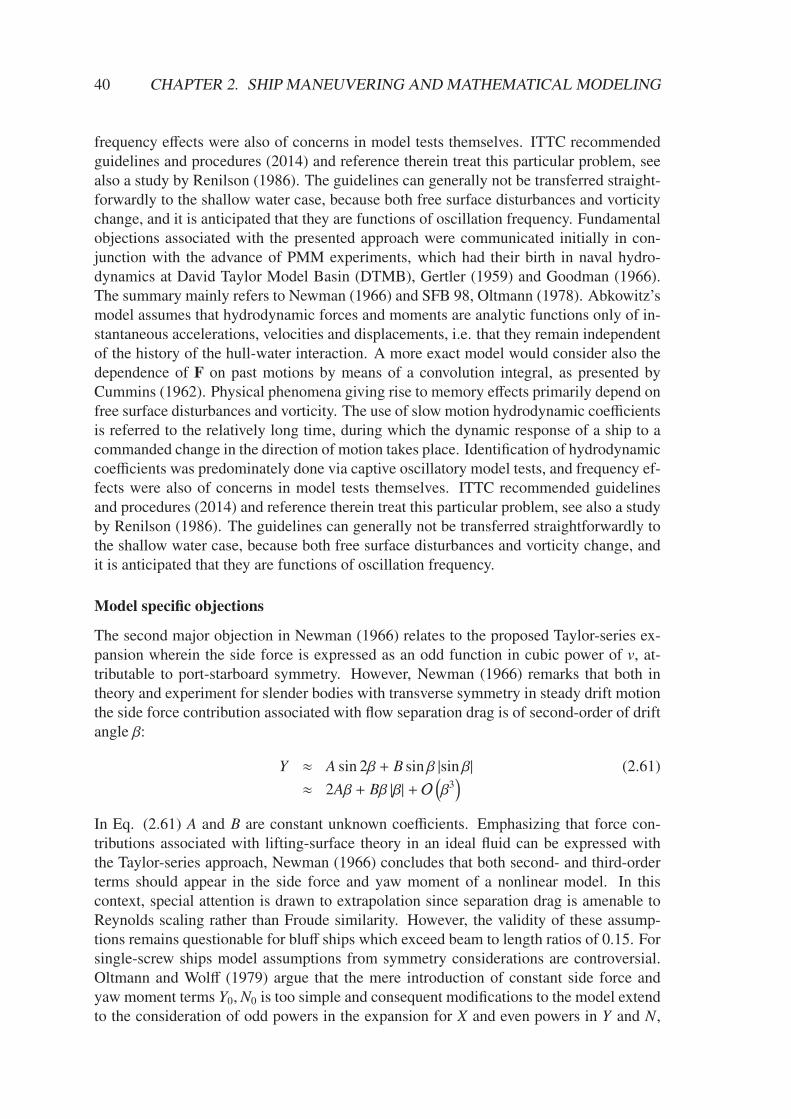
Ship motions in shallow water involve hydrodynamic interactions with vertical flow re-strictions, affecting the dynamic floating position of ships underway and hydrodynamicproperties relating to inertia, lift and cross-flow forces. A detailed treatise of maneuveringforces in shallow water is given in the following, based on the extension of the decom-position of forces for the deep water case. Prior to this discussion, main hydrodynamicinteractions in shallow and confined water are discussed. Hydrodynamic interaction ef-fects in shallow water mean water-depth dependent changes in the pressure field ambientto the ship. These effects can be related to the principle of conservation of energy alonga streamline in ideal flow, postulated by Bernoulli’s equation. According to the Bernoulliequation a decrease in the flow cross-section results in a concurrent increase of the flowvelocity and decrease of pressure. Consequences of Bernoulli’s effect for floating bod-ies are dynamic adjustments of the floating position and orientation. Ships in forwardmotion experience a vertical displacement in the heave mode (sinkage) and a rotationaldisplacement in the pitch mode (trim), accompanied by a decrease of the mean ambientwater level, decreasing UKC, Fig. 2.10. Such decrease in UKC is called squat. Froma ship hydrodynamic point of view, the classification of shallow water flows has to takeinto account a suitable quantity of dimension of velocity. For analysis of forward motionthe Froude depth number Fnh = u/
√
gh has been established. In the sub-critical flow
42 CHAPTER 2. SHIP MANEUVERING AND MATHEMATICAL MODELING
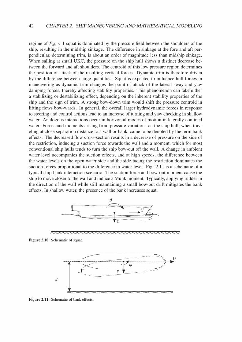
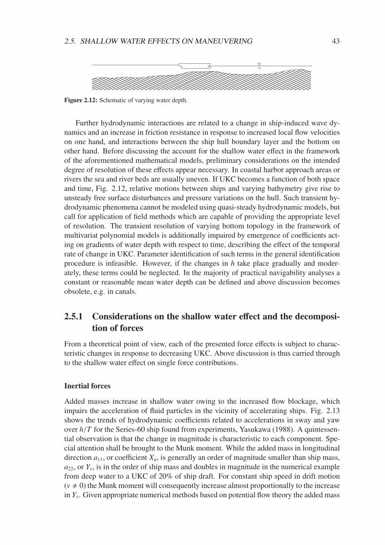
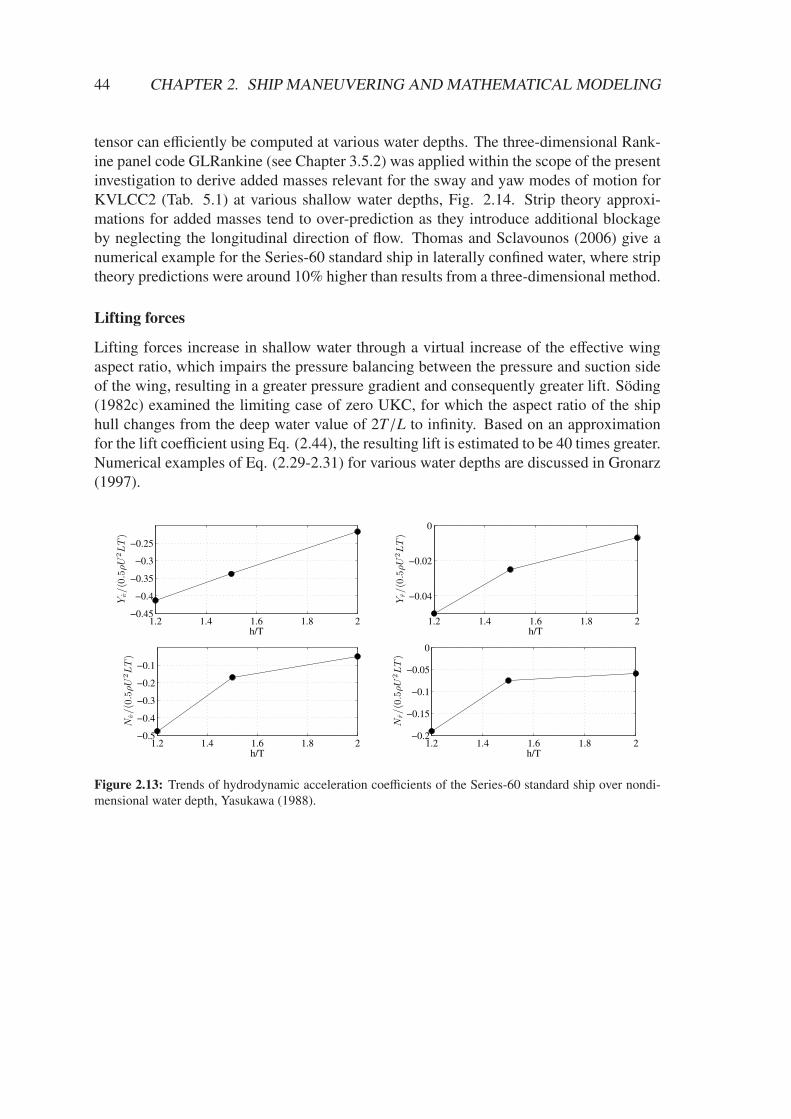
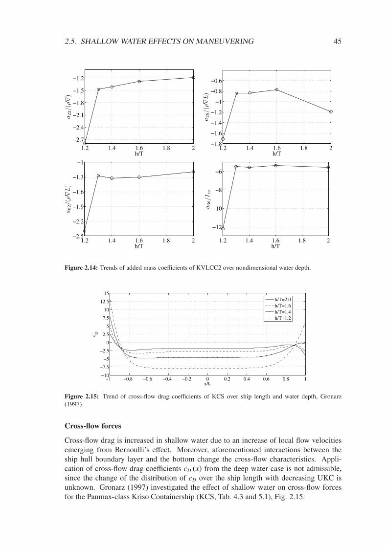
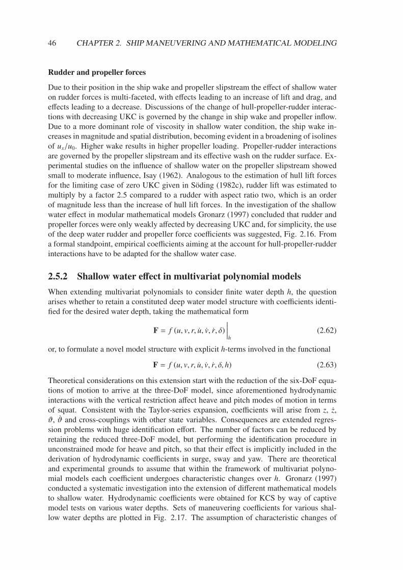
regime of Fnh < 1 squat is dominated by the pressure field between the shoulders of the
ship, resulting in the midship sinkage. The difference in sinkage at the fore and aft per-pendicular, determining trim, is about an order of magnitude less than midship sinkage.When sailing at small UKC, the pressure on the ship hull shows a distinct decrease be-tween the forward and aft shoulders. The centroid of this low pressure region determinesthe position of attack of the resulting vertical forces. Dynamic trim is therefore drivenby the difference between large quantities. Squat is expected to influence hull forces inmaneuvering as dynamic trim changes the point of attack of the lateral sway and yawdamping forces, thereby affecting stability properties. This phenomenon can take eithera stabilizing or destabilizing effect, depending on the inherent stability properties of theship and the sign of trim. A strong bow-down trim would shift the pressure centroid inlifting flows bow-wards. In general, the overall larger hydrodynamic forces in responseto steering and control actions lead to an increase of turning and yaw checking in shallowwater. Analogous interactions occur in horizontal modes of motion in laterally confinedwater. Forces and moments arising from pressure variations on the ship hull, when trav-eling at close separation distance to a wall or bank, came to be denoted by the term bankeffects. The decreased flow cross-section results in a decrease of pressure on the side ofthe restriction, inducing a suction force towards the wall and a moment, which for mostconventional ship hulls tends to turn the ship bow-out off the wall. A change in ambientwater level accompanies the suction effects, and at high speeds, the difference betweenthe water levels on the open water side and the side facing the restriction dominates thesuction forces proportional to the difference in water level. Fig. 2.11 is a schematic of atypical ship-bank interaction scenario. The suction force and bow-out moment cause theship to move closer to the wall and induce a Munk moment. Typically, applying rudder inthe direction of the wall while still maintaining a small bow-out drift mitigates the bankeffects. In shallow water, the presence of the bank increases squat.
ϑ
z
U
Figure 2.10: Schematic of squat.
ψ
y
d
U
Figure 2.11: Schematic of bank effects.
2.5. SHALLOW WATER EFFECTS ON MANEUVERING 43
Figure 2.12: Schematic of varying water depth.
Further hydrodynamic interactions are related to a change in ship-induced wave dy-namics and an increase in friction resistance in response to increased local flow velocitieson one hand, and interactions between the ship hull boundary layer and the bottom onother hand. Before discussing the account for the shallow water effect in the frameworkof the aforementioned mathematical models, preliminary considerations on the intendeddegree of resolution of these effects appear necessary. In coastal harbor approach areas orrivers the sea and river beds are usually uneven. If UKC becomes a function of both spaceand time, Fig. 2.12, relative motions between ships and varying bathymetry give rise tounsteady free surface disturbances and pressure variations on the hull. Such transient hy-drodynamic phenomena cannot be modeled using quasi-steady hydrodynamic models, butcall for application of field methods which are capable of providing the appropriate levelof resolution. The transient resolution of varying bottom topology in the framework ofmultivariat polynomial models is additionally impaired by emergence of coefficients act-ing on gradients of water depth with respect to time, describing the effect of the temporalrate of change in UKC. Parameter identification of such terms in the general identificationprocedure is infeasible. However, if the changes in h take place gradually and moder-ately, these terms could be neglected. In the majority of practical navigability analyses aconstant or reasonable mean water depth can be defined and above discussion becomesobsolete, e.g. in canals.
2.5.1 Considerations on the shallow water effect and the decomposi-
tion of forces
From a theoretical point of view, each of the presented force effects is subject to charac-teristic changes in response to decreasing UKC. Above discussion is thus carried throughto the shallow water effect on single force contributions.
Inertial forces
Added masses increase in shallow water owing to the increased flow blockage, whichimpairs the acceleration of fluid particles in the vicinity of accelerating ships. Fig. 2.13shows the trends of hydrodynamic coefficients related to accelerations in sway and yawover h/T for the Series-60 ship found from experiments, Yasukawa (1988). A quintessen-tial observation is that the change in magnitude is characteristic to each component. Spe-cial attention shall be brought to the Munk moment. While the added mass in longitudinaldirection a11, or coefficient Xu, is generally an order of magnitude smaller than ship mass,a22, or Yv, is in the order of ship mass and doubles in magnitude in the numerical examplefrom deep water to a UKC of 20% of ship draft. For constant ship speed in drift motion(v , 0) the Munk moment will consequently increase almost proportionally to the increasein Yv. Given appropriate numerical methods based on potential flow theory the added mass
44 CHAPTER 2. SHIP MANEUVERING AND MATHEMATICAL MODELING
tensor can efficiently be computed at various water depths. The three-dimensional Rank-ine panel code GLRankine (see Chapter 3.5.2) was applied within the scope of the presentinvestigation to derive added masses relevant for the sway and yaw modes of motion forKVLCC2 (Tab. 5.1) at various shallow water depths, Fig. 2.14. Strip theory approxi-mations for added masses tend to over-prediction as they introduce additional blockageby neglecting the longitudinal direction of flow. Thomas and Sclavounos (2006) give anumerical example for the Series-60 standard ship in laterally confined water, where striptheory predictions were around 10% higher than results from a three-dimensional method.
Lifting forces
Lifting forces increase in shallow water through a virtual increase of the effective wingaspect ratio, which impairs the pressure balancing between the pressure and suction sideof the wing, resulting in a greater pressure gradient and consequently greater lift. Söding(1982c) examined the limiting case of zero UKC, for which the aspect ratio of the shiphull changes from the deep water value of 2T/L to infinity. Based on an approximationfor the lift coefficient using Eq. (2.44), the resulting lift is estimated to be 40 times greater.Numerical examples of Eq. (2.29-2.31) for various water depths are discussed in Gronarz(1997).
1.2 1.4 1.6 1.8 2−0.45
−0.4
−0.35
−0.3
−0.25
Yv/(0
.5ρU
2L
T)
h/T1.2 1.4 1.6 1.8 2
−0.04
−0.02
0
h/T
Yr/(0
.5ρU
2L
T)
1.2 1.4 1.6 1.8 2−0.5
−0.4
−0.3
−0.2
−0.1
h/T
Nv/(0
.5ρU
2L
T)
1.2 1.4 1.6 1.8 2−0.2
−0.15
−0.1
−0.05
0
h/T
Nr/(0
.5ρU
2L
T)
Figure 2.13: Trends of hydrodynamic acceleration coefficients of the Series-60 standard ship over nondi-mensional water depth, Yasukawa (1988).
2.5. SHALLOW WATER EFFECTS ON MANEUVERING 45
1.2 1.4 1.6 1.8 2
−2.7
−2.4
−2.1
−1.8
−1.5
−1.2
h/T
a22/(
ρ∇
)
1.2 1.4 1.6 1.8 2−1.8
−1.6
−1.4
−1.2
−1
−0.8
−0.6
h/T
a26/(ρ∇
L)
1.2 1.4 1.6 1.8 2−2.5
−2.2
−1.9
−1.6
−1.3
−1
h/T
a62/(ρ∇
L)
1.2 1.4 1.6 1.8 2
−12
−10
−8
−6
h/T
a66/I
zz
Figure 2.14: Trends of added mass coefficients of KVLCC2 over nondimensional water depth.
−1 −0.8 −0.6 −0.4 −0.2 0 0.2 0.4 0.6 0.8 1−10
−7.5
−5
−2.5
0
2.5
5
7.5
10
12.5
15
x/L
c D
h/T=2.0
h/T=1.6
h/T=1.4
h/T=1.2
Figure 2.15: Trend of cross-flow drag coefficients of KCS over ship length and water depth, Gronarz(1997).
Cross-flow forces
Cross-flow drag is increased in shallow water due to an increase of local flow velocitiesemerging from Bernoulli’s effect. Moreover, aforementioned interactions between theship hull boundary layer and the bottom change the cross-flow characteristics. Appli-cation of cross-flow drag coefficients cD (x) from the deep water case is not admissible,since the change of the distribution of cD over the ship length with decreasing UKC isunknown. Gronarz (1997) investigated the effect of shallow water on cross-flow forcesfor the Panmax-class Kriso Containership (KCS, Tab. 4.3 and 5.1), Fig. 2.15.
46 CHAPTER 2. SHIP MANEUVERING AND MATHEMATICAL MODELING
Rudder and propeller forces
Due to their position in the ship wake and propeller slipstream the effect of shallow water
on rudder forces is multi-faceted, with effects leading to an increase of lift and drag, andeffects leading to a decrease. Discussions of the change of hull-propeller-rudder interac-tions with decreasing UKC is governed by the change in ship wake and propeller inflow.Due to a more dominant role of viscosity in shallow water condition, the ship wake in-creases in magnitude and spatial distribution, becoming evident in a broadening of isolinesof ux/u0. Higher wake results in higher propeller loading. Propeller-rudder interactionsare governed by the propeller slipstream and its effective wash on the rudder surface. Ex-perimental studies on the influence of shallow water on the propeller slipstream showedsmall to moderate influence, Isay (1962). Analogous to the estimation of hull lift forcesfor the limiting case of zero UKC given in Söding (1982c), rudder lift was estimated tomultiply by a factor 2.5 compared to a rudder with aspect ratio two, which is an orderof magnitude less than the increase of hull lift forces. In the investigation of the shallowwater effect in modular mathematical models Gronarz (1997) concluded that rudder andpropeller forces were only weakly affected by decreasing UKC and, for simplicity, the useof the deep water rudder and propeller force coefficients was suggested, Fig. 2.16. Froma formal standpoint, empirical coefficients aiming at the account for hull-propeller-rudderinteractions have to be adapted for the shallow water case.
2.5.2 Shallow water effect in multivariat polynomial models
When extending multivariat polynomials to consider finite water depth h, the questionarises whether to retain a constituted deep water model structure with coefficients identi-fied for the desired water depth, taking the mathematical form
F = f (u, v, r, u, v, r, δ)∣∣∣∣∣h
(2.62)
or, to formulate a novel model structure with explicit h-terms involved in the functional
F = f (u, v, r, u, v, r, δ, h) (2.63)
Theoretical considerations on this extension start with the reduction of the six-DoF equa-tions of motion to arrive at the three-DoF model, since aforementioned hydrodynamicinteractions with the vertical restriction affect heave and pitch modes of motion in termsof squat. Consistent with the Taylor-series expansion, coefficients will arise from z, z,ϑ, ϑ and cross-couplings with other state variables. Consequences are extended regres-sion problems with huge identification effort. The number of factors can be reduced byretaining the reduced three-DoF model, but performing the identification procedure inunconstrained mode for heave and pitch, so that their effect is implicitly included in thederivation of hydrodynamic coefficients in surge, sway and yaw. There are theoreticaland experimental grounds to assume that within the framework of multivariat polyno-mial models each coefficient undergoes characteristic changes over h. Gronarz (1997)conducted a systematic investigation into the extension of different mathematical modelsto shallow water. Hydrodynamic coefficients were obtained for KCS by way of captivemodel tests on various water depths. Sets of maneuvering coefficients for various shal-low water depths are plotted in Fig. 2.17. The assumption of characteristic changes of
2.5. SHALLOW WATER EFFECTS ON MANEUVERING 47
each coefficient over water depth was confirmed. Most coefficients change in nonlinear
fashion and undergo significant amplification. Coefficients related to rigid body velocities
represent damping terms, including lift and cross-flow effects, which also increase withdecreasing UKC. An additional observation is that with increasing UKC the trend of thecoefficients appears to strive asymptotically towards an anticipated deep water value. Formaneuverability analysis at a desired shallow water depth using multivariat polynomialmodels hydrodynamic coefficients should thus be determined at just this desired waterdepth. In presence of multiple water depth-specific sets of coefficients it is possible toapply regression analysis to approximate a set of coefficients for a water depth which wasnot investigated explicitly, but lays within the range of available data. Gronarz (1997)addressed suitable interpolation schemes, e.g. using cubic splines, but concluded thatleast-squares curve fitting using power functions specific to each coefficient was moreappropriate. This approach takes the form
F = f (u, v, r, u, v, r, δ)︸ ︷︷ ︸
f0
+ fn (T/h)n (2.64)
where f0 refers to the basic deep water functional and fn (T/h) is the shallow water exten-sion in yet to be determined power of T/h. The power functions were shown to providesmooth trends of each coefficient over the water depth and to be suitable to model theasymptotic trend approaching the deep water case. The dependence of hydrodynamicforces on squat on one hand, and the dependence of squat on forward speed on otherhand, brings to the attention the relevance of terms which arise from the expansion of∆u and consider the effect of forward speed changes on F. A concluding remark on thesuitability of multivariat polynomials to model hydrodynamic forces in maneuvering re-lates to the theoretical notion of the frequency-invariance of hydrodynamic coefficientsand the change in inertial response characteristics anticipated for ship maneuvering inshallow water. Ships in confined water are operated at low speeds and experience in-creased hydrodynamic forces acting upon the hull in response to commanded changes indirection. The increase in both inertia and damping forces on the hull increases the timespan during which the state variables in a maneuver vary, or settle to a steady state, whichcaters to the notion of quasi-steady models. In this context, the discussion of forwardspeed perturbation terms deserves a review, because of the generally low forward speedsand anticipated low forward speed losses in shallow water. Challenges arise for the iden-tification of multivariat polynomial models in conjunction with the flow restriction andhydrodynamic interactions (squat) in captive maneuvering tests. In experimental shallowwater towing tank setups finite tank dimensions add to the flow blockage, and the setupis prone to be affected by wave reflection initiated in the acceleration phase of the model.These effects are to be seen as a constraining factor for the choice of prescribed motionparameters in surge, sway and yaw. Particularities and challenges of identification andregression analysis will be addressed later.
48 CHAPTER 2. SHIP MANEUVERING AND MATHEMATICAL MODELING
−40 −20 0 20 40
−3
−2.5
−2
−1.5
−1
−0.5
0x 10
−4
δ [°]
X′
−0.4 −0.2 0 0.2 0.40
0.2
0.4
0.6
0.8
1
1.2x 10
−3
v′
X′
−0.4 −0.2 0 0.2 0.40
0.2
0.4
0.6
0.8
1x 10
−4
r′
X′
h/T=1.2
h/T=1.4
h/T=1.6
h/T=2.0
−40 −20 0 20 40−8
−5.5
−3
−0.5
2
4.5
78
x 10−4
δ [°]
Y′
−0.4 −0.2 0 0.2 0.4−0.05
−0.025
0
0.025
0.05
v′
Y′
−0.4 −0.2 0 0.2 0.4−8
−6
−4
−2
0
2
4
6
8x 10
−4
r′
Y′
h/T=1.2
h/T=1.4
h/T=1.6
h/T=2.0
−40 −20 0 20 40−4
−2
0
2
4x 10
−4
δ [°]
N′
−0.4 −0.2 0 0.2 0.4−0.01
−0.005
0
0.005
0.01
v′
N′
−0.4 −0.2 0 0.2 0.4−2
−1
0
1
2x 10
−3
r′
N′
h/T=1.2
h/T=1.4
h/T=1.6
h/T=2.0
Figure 2.16: Hydrodynamic forces of KCS as a function to rudder angle, sway velocity and yaw rate for
various water depths, Tab. 8.2, Gronarz (1997).
2.5. SHALLOW WATER EFFECTS ON MANEUVERING 49
1 1.5 2 2.5 3 3.5 4−300
−250
−200
−150
−100
h/T
Xu
1 1.5 2 2.5 3 3.5 480
100
120
140
160
h/T
Xu
u
1 1.5 2 2.5 3 3.5 40
500
1000
1500
h/T
Xvr
1 1.5 2 2.5 3 3.5 4−4000
−3000
−2000
−1000
0
h/T
Yv
1 1.5 2 2.5 3 3.5 4−3
−2
−1
0x 10
4
h/T
Yv|v|
1 1.5 2 2.5 3 3.5 450
75
100
125
150
h/T
Yδ
1 1.5 2 2.5 3 3.5 450
100
150
200
250
h/T
Yr
1 1.5 2 2.5 3 3.5 4−250
−200
−150
−100
−50
h/T
Yrrr
1 1.5 2 2.5 3 3.5 4−5000
0
5000
10000
h/T
Yrvv
1 1.5 2 2.5 3 3.5 4−10000
−7500
−5000
−2500
0
h/T
Yvrr
1 1.5 2 2.5 3 3.5 4−1500
−1250
−1000
−750
−500
h/T
Nv
1 1.5 2 2.5 3 3.5 4−3000
−2000
−1000
0
h/T
Nv|v|
1 1.5 2 2.5 3 3.5 4−80
−60
−40
−20
h/T
Nδ
1 1.5 2 2.5 3 3.5 4−500
−400
−300
−200
−100
h/T
Nr
1 1.5 2 2.5 3 3.5 4−200
−175
−150
−125
−100
h/T
Nrrr
1 1.5 2 2.5 3 3.5 4−6000
−4000
−2000
0
h/T
Nrvv
1 1.5 2 2.5 3 3.5 4−1500
−1000
−500
0
500
h/T
Nvrr
Figure 2.17: Hydrodynamic maneuvering coefficients of KCS over nondimensional water depth multiplied
by 1000, Gronarz (1997).
50 CHAPTER 2. SHIP MANEUVERING AND MATHEMATICAL MODELING
2.6 Linear equations of motion and straight line stability
analysis
For maneuvering problems involving small deviations in sway and yaw from a mean ship
trajectory constant cruise speed (U ≈ U0) can be assumed and a sway-yaw-subsystemmodel can be established. The linear time-invariant framework of maneuvering dynamicsenables classic investigation of inherent system stability properties, which are useful forgeneral maneuvering performance evaluation, e.g. straight line motion stability. If onlylinear terms are retained, the maneuvering equations of motion can be rewritten as
Mx + Nx = FRδ (2.65)
M =
[
−Yv + m −Yr + mxg
−Nv + mxg −Nr + Iz
]
N =
[
−Yv −Yr + mU0
−Nv −Nr + mxgU0
]
x = [v r]T
FR = [Yδ Nδ]T
with state vector x (t), mass and inertia matrix M, hydrodynamic damping matrix N, andrudder force vector FR, constituting a classic mass-damper system. The latter can readilybe arranged in state-space representation for time-invariant linear systems with systemmatrix A = −M−1N, input vector B =M−1F and input u (t) = δ
x(t) = Ax(t) + Bu(t) (2.66)
with general solution
x(t) = eAtx(0) +∫ t
0eA(t−τ)Bu(τ) dτ (2.67)
In absence of controls Eq. (2.67) reduces to
x(t) = eAtx0 (2.68)
and the inherent stability behavior of the dynamic system can be studied by turning tothe eigenvalues λ of A, where eigenvalues with positive real part, ℜ(λ) > 0, give wayto unbounded amplification in response to arbitrary external excitations. It can be shownfrom evaluation of the characteristic polynomial
|A − λI| = 0 (2.69)
|M| λ2 − (A11 + A22) λ +|N||M|2
= 0 (2.70)
and by application of Vieta’s rule that stability is guaranteed for
− (A11 + A22)|M| > 0 ∧ |N|
|M|3> 0 (2.71)
2.7. PARAMETER IDENTIFICATION 51
where
A11 = −1
|M|
∣∣∣∣∣∣
M22 M12
N21 N11
∣∣∣∣∣∣; A22 = −
1
|M|
∣∣∣∣∣∣
M11 M21
N12 N22
∣∣∣∣∣∣
(2.72)
The l.h.s. criterion is always met, because both − (A11 + A22) and |M| are always positive
for ships, which leaves the stability criterion rest with the sign of the determinant of the
damping matrix, which after rearrangement of terms yields
|N| = Yv (Yr − mU0)
(Nr − mxgU0
Yr − mU0
− Nv
Yv
)
> 0 (2.73)
The analysis of hydrodynamic coefficients related to damping
Yv < 0; Nr < 0; Nv < 0; Yr > 0 (2.74)
reveals that Yv (Yr − mU0) is always positive. In general, the sign of Nv is ambiguous,
as it can indeed be a (albeit small) positive value. The nature of the arrangement of
terms in the damping matrix enables an illustrative discussion from a physical standpoint,
Abkowitz (1964), Söding (1982c). Rearrangement of terms in Eq. (2.73) allows the
expression in terms of the point of attack of the lateral yaw damping force with respect to
the longitudinal axis x as
lr =Nr − mxgU0
Yr − mU0
(2.75)
and the point of attack of the lateral sway damping force with respect to axis x as
lv =Nv
Yv(2.76)
which furnishes the discussion of straight line stability with the general conclusion that a
ship is stable, if the lateral yaw damping force attacks ahead of the lateral sway damping
force
lr > lv (2.77)
Available water depth-dependent hydrodynamic coefficients (Fig. 2.17) for KCS wereused to study the shallow water effect on straight line stability. Results are organized in aplot showing the ratio lr/lv over h/T , Fig. 2.18. A value of one indicates the above definedstability threshold.
2.7 Parameter identification
The presented mathematical models include unknown ship-specific parameters, which inabsence of analytic methods for determination require experiments for identification. Pa-rameter identification procedures encompass the design of experiments in accordance withthe mathematical model, the conduction of the experimental programme and a suitablemathematical method to synchronize experimental results with the mathematical model.This section deals with identification procedures for multivariat polynomial models rely-ing on captive maneuvering tests on idealized trajectories, albeit large parts of the pre-sented methodology are also applicable to other maneuvering models. In the ship hydro-dynamic community a differentiation has been established between so-called indirect anddirect parameter identification, which will be defined in the remainder.
52 CHAPTER 2. SHIP MANEUVERING AND MATHEMATICAL MODELING
1 1.5 2 2.5 3 3.5 40
0.2
0.4
0.6
0.8
1
1.2
1.4
1.6
1.8
h/T
l r/lv
Figure 2.18: Straight line stability analysis for KCS over nondimensional water depth.
2.7.1 Indirect parameter identification in ship maneuvering
Indirect parameter identification draws upon measurements from free-running maneuver-ing tests available from either sea trials or scale model experiments. In free-running ma-neuvering tests, the transient position of the ship or ship model (and deducible derivatives)are tracked, and the histories of inputs to the dynamic system (rudder angle, propeller rateof revolution, etc.) are recorded. Different algorithms are in place to adjust the unknownmodel parameters as to fit the experimental data in optimal fashion, e.g. the method pro-posed by Kudva and Narendra (1974). Such algorithms predominately seek to minimizeerrors of the simulated prediction compared to the source test data, but require a fairlygood estimate of the entire set of coefficients as a starting point for the iterative proce-dure. Oltmann (1978) provides examples for applications to ship maneuvering.
2.7.2 Direct parameter identification in ship maneuvering
Direct parameter identification follows a regression analysis of forces and moments froma host of captive maneuvering test on idealized trajectories. The model of the ship istowed on either straight path with prescribed rudder or drift angle, or in steady turningmotion. Additionally, pure sway, pure yaw, combined sway-yaw or yaw oscillations withsteady drift angle are run. The experimental setup allows for a prescribed constraining ofparticular modes of motion. Fig. 2.19 is a schematic of a typical CPMC device, Grim etal. (1976). The figure shows a longitudinal section of the towing tank and the alignmentof the CPMC.
2.7.3 Remarks on scale effects
While the experimental direct parameter identification approach is confined to model scaleship flows, CFD-based replications can handle both model and full scale investigations.However, such simulations are still performed for model scale only to ensure a commonbasis for validation of force computations through comparison with model experiments.
2.7. PARAMETER IDENTIFICATION 53
V
Figure 2.19: Schematic of a CPMC device, Grim et al. (1976).
Extrapolation to full-scale maneuvering predictions relies on Froude similarity. Notwith-standing the fact that the majority of force effects in maneuvering are expected to bepressure-dominated, a discussion of scale effects appears necessary for the framework ofthe present investigation. CFD is increasingly being used to gain more insights into scaleeffects involved in maneuvering. El Moctar et al. (2014) give a summary on anticipatedinfluences on maneuvering due to different Reynolds number flows. Main scale effects areassociated with different wake numbers, the lack of a friction deduction force in maneu-vering experiments and different engine characteristics. These effects will differ betweensingle-screw and twin-screw ships. For a single-screw ship, the higher wake number andpropeller loading have opposite effects on rudder forces. Ideally, the errors cancel com-pletely. For a twin-screw ship, the wake effect is weak as the propellers operate in morehomogeneous flow. The propeller loading effect remains for twin-screw ships. Hence,twin-screw ships are assumed to have stronger scale effects. Recent studies in deep waterconditions reveal experimental evidence that scale effects involved in ship maneuveringin deep water remain moderate, Lantermann et al. (2015).
2.7.4 Analysis of captive steady motion tests
Linear curve fitting based on least-squares minimization is the predominate choice toanalyze captive steady motion tests. The classic linear regression problem of generalizedform is stated as
Φi = f (xi)a + ǫi i = 1, 2, ...N (2.78)
where Φi is response of experiment i, f (xi) vector of regressors, x vector of factors, a
vector of regression parameters and ǫi random measurement error. Captive static maneu-vering tests comprise a host of steady motion runs in which one or more parameters arevaried over a desired number of factors
x = [x1, x2, ..., xm]T (2.79)
In experiments time histories of forces and moments of each run are averaged to givesteady state results. Repeatability studies involve statistical evaluation. In steady CFD
54 CHAPTER 2. SHIP MANEUVERING AND MATHEMATICAL MODELING
simulations results are used after satisfaction of a defined convergence criterion of a single
simulation, not involving random scatter. These results populate response vector Φ
Φ = [Φ1,Φ2, ...,ΦN]T (2.80)
Usually, the number of responses m is greater than the number of unknown parameters n,
but at least has to be equal. In least-squares approaches, unknown regression parameters
a = [a0, a1, ..., an]T (2.81)
are found by minimizing the residual vector using the Euclidean norm
min∥∥∥AaT −Φ
∥∥∥
2
2(2.82)
to give the system of linear equations
AT Aa = ATΦ (2.83)
where A is called design matrix and composed according to
as Moore-Penrose inverse of A. The goodness of the fit is checked by coefficient of deter-mination R2
R2 =
∑Ni=1( f (xi, a) − Φ)2
∑Ni=1(Φi − Φ)2
(2.86)
and
Φ =1N
N∑
i=1
Φi (2.87)
R2 of 1 means all data points actually lay on the curve fit. Upper and lower bounds ofconfidence pcb for computed factors within above framwork can be obtained by
pcb = a ± t√
S (2.88)
where a is the fitted coefficient, t is a factor based on Student’s distribution function andthe anticipated confidence level - a common choice is 95% - and S stems from the productof the diagonal elements of the variance matrix and mean-square error. The differencebetween the lower and upper confidence bounds indicate the level of uncertainty involvedin the curve fitting.
2.7. PARAMETER IDENTIFICATION 55
a) b)
c) d)
yAψA
Figure 2.20: Schematic of captive maneuvering tests: a) Pure sway, b) Pure yaw, c) Yaw with drift, d)
Sway-yaw (asynchronous)
2.7.5 Analysis of captive dynamic motion tests
Captive dynamic maneuvering tests are prescribed harmonic motions in sway, yaw, ora combination of sway-yaw superposed to steady forward motion. Fig. 2.20 illustratesthe trajectories and orientation of the model in pure sway, pure yaw, sway-yaw (hereasynchronous) or yaw oscillation with fixed drift angle. Above motions are characterizedby parameters:
ω′ =ωL
Uc(2.89)
v′ = yAω′ (2.90)
r′ = ψAω′ (2.91)
where ω′ is nondimensional frequency of oscillation stemming from ω = 2π/T , where Tis oscillation period. Steady forward speed of the carriage device is Uc, yA is the maximumtransverse displacement of the prescribed harmonic trajectory and ψA is the maximumyaw angular displacement. ITTC (2014) provides recommendations for the choice ofnondimensional frequency ω′. For dynamic tests the periodic time series of measured orcomputed forces are subjected to Fourier analysis to give force contributions in-phase andout-of-phase with the trajectory. The underlying assumption is that the force record is2π-periodic and can be approximated by the Fourier series
f (t) = a0 +
∞∑
k=1
(ak cos kt + bk sin kt) (2.92)
with coefficients
a0 =1T
∫ T
0f (t) dt (2.93)
ak =2T
∫ T
0f (t) cos kt dt (2.94)
bk =2T
∫ T
0f (t) sin kt dt (2.95)
56 CHAPTER 2. SHIP MANEUVERING AND MATHEMATICAL MODELING
Two methods can be employed for the tests, i.e. the so-called multiple-run and the single-run method. Following the multiple-run method coefficients are found from processingdata from a series of tests over a range of frequencies. Coefficients for the mathemati-cal model are then found by extrapolation to zero-frequency. Fig. 2.21 illustrates resultsfor first-order hydrodynamic coefficients related to inertia and damping from a series ofpure sway motion tests with a spheroid of typical ship dimensions, Mucha and el Moctar(2013). The l.h.s. plot shows Yv as a function of ω2 and for two amplitudes yA. Yv takeshigher norm values the smaller the frequency gets, this trend approaches the referencevalue of a22/(ρ∇) from potential flow theory, Newman (1978). The lowest frequency cor-responds to the smallest ITTC recommendation ω′ = 0.25 and the highest frequency isequivalent to ω′ = 4. Results scatter around the reference value by maximum 5%. Ther.h.s. plots show the Fourier decomposed force contributions without normalization as afunction of sway velocity yAω and acceleration yAω
2. By varying the frequency mem-ory effects and nonlinearities involved in the test procedure can be identified, Renilson(1986). The difference between the amplitude curves indicates memory effects. The devi-ation of these curves from a straight line reveals nonlinearities. In the single-run methoddata from a single run are evaluated. Both motion amplitude and oscillation frequency aresubject to constraints, e.g. finite tank dimensions. In general, frequencies must be chosenin accordance with the underlying mathematical model, which by virtue of the conceptof slow-motion hydrodynamic coefficients prohibits the use of high frequencies. To cir-cumvent non-stationary lift and memory effects a maximum ω′ of typically 1-2 for swayand 2-3 for yaw tests is recommended. Comparable values result from considerationson lateral wake patterns. Considerations on errors in the accuracy of the trajectory yieldcompromise values for ω′ in the range of 2-4 for yaw tests, and 0.25-2 for pure sway tests.Additionally, the circular frequency must not be selected in the vicinity of the eigenfre-quency of the carriage and measurement system. The same applies to possible resonancewith the water in the tank to avoid standing waves. The number of oscillations per test runis again limited by tank dimensions, but should at least be three. In the practical parame-ter identification setup this guideline almost exclusively prevailed over inference of moresophisticated established identification procedures stemming from system theory, whichensure mathematically that input signals were suitable for the excitation of the dynamicsof the system and ensure convergence of the parameter identification procedure, Kudvaand Narendra (1974) and Yuan and Wonham (1977). In general, for common ship modelsizes between 5-7 m in length, satisfactory practical experience was gained with motionperiods around T = 20 s, Wolff (1981), Cura (2008). First-order force contributions mightbe determined from low-amplitude tests, e.g. v′ ≤ 0.1, r′ ≤ 0.4. For higher-order contri-butions large-amplitude tests must be performed to excite nonlinearities in the responsesto prescribed motions, e.g. v′ ≥ 0.25, r′ ≥ 0.5. Special attention is referred to applicationof captive tests in shallow water, where flow blockage gives rise to dynamic sinkage andtrim of ship models, which limits the range of motion amplitudes. Also, the different na-ture of free surface disturbances brings to the attention the questions of memory effects,and the expected change of flow characteristics with respect to viscosity raises concernsabout the validity of Froude scaling.
2.7. PARAMETER IDENTIFICATION 57
0 1 2 3 4 5 6 7 8
x 10−3
−0.98
−0.97
−0.96
−0.95
−0.94
−0.93
−0.92
−0.91
−0.9
ω2 [rad/s2]
Yv/(ρ∇
)
yA
=1m
yA
=2m
Potential flow theory
0 1 2 3 4 5 6 7 8
x 10−3
−0.07
−0.06
−0.05
−0.04
−0.03
−0.02
−0.01
0
Yv/(0
.5ρB
TU
2)
yAω2 [m/s2]0.03 0.04 0.05 0.06 0.07 0.082
2.5
3
3.5
4
4.5
5
5.5
6x 10
−3
Yv/(0
.5ρB
TU
2)
yAω [m/s]
Figure 2.21: Frequency dependence study on hydrodynamic coefficients of a spheroid.
Table 2.1: Required number of test runs in different experimental designs, Sutulo and Guedes Soares
Efficient setups of maneuvering tests can be achieved through application of the theory ofthe experimental design and optimization, Hahn (1984) and Steinberg and Hunter (1984).Sutulo and Guedes Soares (2002) provide a discussion on this theory and extend it to theapplication of optimized designs for ship maneuvering experiments. The present treatiseis based on these references. In light of the need for a database of responses to performthe presented linear regression analysis, the problem emerges of rapidly increasing exper-imental costs with increasing number of independent variables (factors), if the intuitiveconcept of one-factor-at-a-time variation is applied using a certain number of test runs(levels) for each factor. Such designs are called full-factorial designs. If only a few fac-tors are involved, e.g. transverse velocity v, yaw rate r and rudder angle δ (i.e. threefactors), the additional experimental cost of full-factorial designs will be moderate. How-ever, if more factors are involved, e.g. forward speed u and water depth h (i.e. five factors)full-factorial designs become uneconomic. A first step to economic designs is the explo-ration of mathematical properties of the particular regression problem, e.g. a third-orderpolynomial requires the least-squares evaluation of (just) four responses. However, gen-erating more responses would serve as redundancy and feedback on the validity of theunderlying model assumptions. Such designs are called saturated designs. Tab. 2.1 istaken from Sutulo and Guedes Soares (2002) to illustrate the problem in terms of requirednumber of test runs for various design concepts and factors. The number of responses
58 CHAPTER 2. SHIP MANEUVERING AND MATHEMATICAL MODELING
N to be generated by an experimental programme is linked to the number of regression
coefficients n by
N = νn (2.96)
where ν is called redundancy factor. Consistent with introductory discussions ν = 1 is
the saturated design and hence, ν ≥ 1 always. The concept of the optimized experimental
design is to find the optimal distribution of test parameter combinations (factor points) in
the design domain. Among the various optimization criteria available, the so-called D-optimality has received special attention, Sutulo and Guedes Soares (2002). The referenceleans on the pioneering contributions of the general theory of experimental design andoptimization algorithms, e.g. Mitchell (1974) and Welch (1984). The D-criterion seeks tominimize the average variance of the regression parameter estimates, i.e. minimizing themagnitude of the determinant of the variance matrix
min D = min(
AT A)−1
(2.97)
Particular challenges in the optimization are the performance of the actual iterative searchalgorithm and the selection of initial conditions required to solve the optimization prob-lem . Sutulo and Guedes Soares (2002) demonstrated the efficacy of D-optimized exper-imental designs for a typical maneuvering model with 20 unknown coefficients relatingto three factors β, r and δ, which achieved an eight- to nine-fold saving in the number oftest runs compared to a full-factorial design without significantly trading accuracy of theregression.
3. Numerical Fluid Dynamics for Ship
Flows
The analysis of fluid motions stems from the mass, momentum and energy conservation
equations based on principles of classic continuum mechanics and the generalized trans-port theorem. It is represented mathematically by a set of partial differential equations.Variations of flow variables transported through a given control domain are seen to bedriven by convection, diffusion and sources or sinks within the control domain. For flowsaround ship the formulation of these equations is relevant for either water only, or formulti-phase flows including air. Upon determination of the flow variables velocity andpressure, integral quantities like forces and moments on ships can be deduced, whichenable the computation of rigid body motions in fluids. This chapter presents the fun-damental concepts of modeling fluid dynamics for flows around ships, encompassing thediscussion of the mathematical framework and techniques for numerical solution withCFD and a Rankine panel Boundary Element Method (BEM). Fundamentals of fluid dy-namics and numerical methods are mainly summarized from Fox et al. (2010), Ferzigerand Peric (2002) and Newman (1978).
3.1 Definitions and frames of reference
Fluid dynamics are formulated for an earth-fixed inertial reference frame in a Cartesian co-ordinate system. The x-axis points upstream, the y-axis leftward and the z-axis is directedupwards. The longitudinal fluid particle velocity is denoted by u, transverse velocity v andvertical velocity w. Cartesian positions are included in vector x. The fluid velocity vectoris denoted v. Conservation equations are formulated in Eulerian sense for an arbitrarycontrol volume (CV) enclosed by surface S and fixed in space. Face normals n point outof CVs. When appropriate, index notation is used, where xi refers to Cartesian coordinatesx, y, z and vi to the Cartesian components of velocity vector v, where i = 1, 2, 3.
3.2 Classification of fluid flows for ship hydrodynamics
Prior to formulating flow equations a basic classification of fluids based on their prop-erties is made to find simplified mathematical descriptions tractable for solution within
60 CHAPTER 3. NUMERICAL FLUID DYNAMICS FOR SHIP FLOWS
reasonable time in an engineering context. Flows around ships can be assumed incom-pressible, which states that the ratio of a characteristic fluid velocity u and speed of soundus, called Mach number and denoted by M = u/us, is not greater than 0.3. In incompress-ible flows fluid density is constant. For gas phases common speed ranges of ships alsoyield incompressible flows, and it is a reasonable assumption to take air as an ideal gas.Real fluid flows are viscous. The presence of shear stresses between two fluid particlesrequires steadiness of the tangential velocity between them. At solid boundaries this re-sults in equal velocities of the boundary and the fluid on the boundary surface. Viscousflow is formulated for Newtonian fluids, assuming that shear stresses are a linear functionof the wall tangential fluid velocity. Another feature of flows around ships is turbulence.Turbulent flows exhibit random velocity fluctuations in space and time. Both the influ-ence of viscosity and turbulence can be related to the ratio of kinetic to viscous energy,called Reynolds number and denoted by Re = uL/ν, where L is characteristic length andν kinematic fluid viscosity. However, for a host of problems in ship hydrodynamics theviscous wall boundary layer is relatively thin and it is a reasonable approach to assume in-viscid flow, reducing the computational cost of numerical solutions considerably. Finally,ship flows include waves, the prediction of which requires a formulation for the watersurface elevation in space and time, too. Ship waves are gravity surface waves, which arerelated to the ratio of kinetic to gravitational energy, called Froude number and denotedby Fn = u/
√gL.
3.3 Formulation of fluid motions
The starting point is the formulation of conservation of mass and momentum. In integralvector notation the mass conservation equation reads
ρ∂
∂t
∫
V
dV + ρ
∫
S
v · n dS = 0 (3.1)
In incompressible flows the first term in Eq. (3.1) is zero. However, it is retained here,because it becomes non-zero for moving grid problems which will be discussed later. Eq.(3.1) is called the continuity equation. The conservation of momentum is given by
ρ∂
∂t
∫
V
v dV + ρ
∫
S
(vv) · n dS =
∫
S
T · n dS + ρ
∫
V
b dV (3.2)
In Eq. (3.2), b is a vector describing a force per unit mass and T denotes the stress tensor
T = pI + τ (3.3)
where p is pressure and τ the shear stress tensor, which in Cartesian component and indexnotation reads
τi j = µ
(
∂vi
∂x j+∂v j
∂xi
)
(3.4)
where µ is dynamic viscosity. Eq. (3.1-3.2) form the Navier-Stokes equations.
3.3. FORMULATION OF FLUID MOTIONS 61
3.3.1 Turbulence
Turbulent flows are characterized by fluctuations in space and time over a wide range of
scales. A dominant property is the mix of transported flow quantities, called turbulent
diffusion, because it is responsible for the reduction of kinetic energy. An accurate nu-merical prediction of turbulent transport of momentum has to encompass the resolutionof turbulence-induced eddies of all scales, which can be achieved by solving the Navier-Stokes equations free of any approximations, other than those needed for numerical so-lution, called Direct Numerical Simulation (DNS). DNS requires a fine discretization ofcomputational domains and is computationally expensive. To reduce this cost approxima-tions for small-scale turbulent structures can be introduced, while large-scale fluctuationsare still resolved within the exact framework of flow equations. This approach is knownas Large Eddy Simulation (LES). Further trading accuracy against cost, a general aver-aging of flow equations with respect to time, space or a set of flow realizations can bedone. This method refers to Reynolds-averaged Navier Stokes (RANS) equations and hasbecome the choice over DNS and LES for the majority of analyses of flows around ships.Assuming a statistically steady flow the velocity and pressure field can be expressed asthe sum of a mean value and its fluctuation, here given symbolically by φ
φ (x, t) = φ (x, t) + φ′ (x, t) (3.5)
where
φ (x, t) =1T
∫ T
0φ (x, t) dt (3.6)
andφ (x, t)′ = 0 (3.7)
The time intervall T ideally runs to infinity but must be sufficiently large compared tothe fluctuation time scale. In unsteady flows, the mean value is found from ensembleaveraging
φ (x, t) =1N
N∑
n=1
φn (x, t) (3.8)
where the number of ensembles N ideally runs to infinity but must be sufficiently largeto compensate fluctuation effects. Upon introduction to the Navier-Stokes equations, itfollows
ρ∂
∂t
∫
V
dV + ρ
∫
S
v · n dS = 0 (3.9)
∂
∂t
∫
V
ρv dV +
∫
S
ρ(
v v + v′v′)
· n dS =
∫
S
T · n dS +
∫
V
ρb dV (3.10)
The emerging ρv′iv′j terms are known as the Reynolds stresses. The averaging of the prod-
uct of these fluctuations does not cancel them out because their correlation function cantake a non-zero value. The presence of these terms leads to the so-called closure problem.For practical applications approximations have been formulated. These predominatelydraw upon semi-empirical approaches like the concept of eddy viscosity. Eddy viscosity
62 CHAPTER 3. NUMERICAL FLUID DYNAMICS FOR SHIP FLOWS
models base on the assumption that turbulent effects can be considered as to act like in-creased viscosity, which in mathematical sense leads to equations of equivalent form asthe viscous stresses
ρv′iv′j = −µt
(
∂vi
∂x j+∂v j
∂xi
)
+23δi jρk (3.11)
and
v′iφ′ = −Γt
∂φ
∂xi(3.12)
where µt is turbulent eddy viscosity, k is turbulent kinetic energy, Γt is turbulent diffusioncoefficient and δi j is Kronecker delta. Turbulent viscosity and diffusivity are defined as:
µt = Cµρk2
ǫ(3.13)
andΓt =
µt
σφ
(3.14)
where σφ is the turbulent Schmidt number which is determined empirically. Two transportequations need to be solved to obtain k and ǫ:
∂ (ρk)∂t+∂(
ρv jk)
∂x j=
∂
∂x j
((
µ +µt
σk
)
∂k
∂x j
)
+ Pk − ρǫ (3.15)
∂ (ρǫ )∂t
+∂(
ρv jǫ)
∂x j= Cǫ1Pk
ǫ
k− ρCǫ2
ǫ2
k+
∂
∂x j
(
µt∂ǫ
σǫ∂x j
)
(3.16)
where Pk is turbulent production rate, σǫ is turbulent dissipation number and Cǫ1 and Cǫ2
are nondimensional coefficients quantified in Launder and Spalding (1974). This modelis known as the kǫ-model. Another widespread turbulence model which involves twoadditional transport equations is the kω-model. Here, ω is specific turbulent dissipation.The two transport equations for k and ω read
∂ (ρk)∂t+∂(
ρv jk)
∂x j= Pk − ρβ∗kω +
∂
∂x j
[(
µ +µt
σ∗k
)
∂ω
∂x j
]
(3.17)
∂ (ρω )∂t
+∂(
ρv jω)
∂x j= αPk
ω
k− ρβω2 +
∂
∂x j
[(
µ +µt
σ∗ω
)
∂ω
∂x j
]
(3.18)
with turbulent Prandtl numberσk and coefficients β, β∗ and α, quantified in Wilcox (1988).Within this concept turbulent eddy viscosity is proportional to the ratio of turbulent kineticenergy and specific dissipation:
µt ∝k
ω(3.19)
Menter (1994) developed the shear stress transport (SST) kω-model which seeks to com-bine the benefits of the kω- and kǫ-models by switching between them in the free-streamand near-wall region. Special attention is brought to the near-wall treatment of flowequations, and associated discretization and solution procedures. In light of high and
3.3. FORMULATION OF FLUID MOTIONS 63
anisotropic fluctuations of turbulent flow variables in the vicinity of walls, a very fine
grid resolution normal to the boundary becomes necessary when pursuing to integrate the
RANS-equations down to the wall. For high Reynolds number flows with a thin viscoussub-layer fine near-wall grid resolution and the resulting increase in computational effortis unfavorable. In near-wall turbulence modeling, wall functions are alternatively used tocircumvent this problem. Wall functions base on the assumption of a logarithmic velocityprofile normal to the wall:
u+ =um
√
|τw| /ρ=
1κ
ln(
y+)
+ B (3.20)
where um is mean wall-parallel velocity, τw wall shear stress, κ von Kármán’s constant, y+
nondimensional wall distance, defined as
y+ =ρy
√
|τw| /ρµ
(3.21)
with y the distance from the wall to the first cell computation point and B a roughnesscoefficient. Wall-functions are referred to high y+, or high Reynolds number models.Linear eddy viscosity models have been shown to yield deviations in predicting local andintegral flow quantities in presence of vorticity generation from turbulence anisotropywhich is pronounced for hulls with distinct streamline curvature, Deng and Visonneau(1999, 2005). Reynolds stress models (RSM) abandon the eddy viscosity concept andseek to compute the stress tensor directly, Launder et al. (1975). Application of RSM isoften impaired by numerical stability problems. Rodi (1976) proposed an algebraic stressmodel (ASM) stemming from the so-called weak equilibrium condition and including anonlinear treatment of the production-to-dissipation rate ratio. Issues regarding robustnesshave been circumvented by an explicit solution scheme, Gatski and Speziale (1993). Dengand Visonneau (2005) discuss the application of explicit algebraic stress models (EASM)to flows around ship. Discussions of turbulent flows are presented in detail in Pope (2000).
3.3.2 Pressure coupling
The momentum conservation equations contain the pressure gradient ∇p, but a separateequation to be solved for the pressure is missing. A solution to the problem can be foundfrom the application of projection methods, Chorin (1967). Projection methods decouplethe computation of the velocity and pressure field making use of Helmholtz decompo-sition. The fundamental idea behind Helmholtz decomposition is to look upon a givenvector field as the sum of a divergence-free and an irrotational vector field. Following thisnotion an intermediate velocity field is determined, which at this point does not satisfy thecontinuity equation, but can be used to map the pressure onto the divergence-free velocityfield and correct the velocity and pressure thereafter. The divergence of the momentumconservation equation in conjunction with the continuity equation can be used to derive aPoisson type equation for pressure of the form
∂
∂xi
(
∂p
∂xi
)
= − ∂
∂xi
∂(
ρviv j
)
∂x j
(3.22)
64 CHAPTER 3. NUMERICAL FLUID DYNAMICS FOR SHIP FLOWS
Instead of this equation the solution method implemented in the solver described in Sec-tion 3.5.1 uses a pressure-correction equation which is derived from the discretized conti-nuity and momentum equations following the Semi-Implicit Method for Pressure-linkedEquations (SIMPLE) algorithm proposed by Caretto et al. (1972). A compact summaryof the iterative solution procedure for incompressible flows is as follows:
1. Solve the linearized momentum equations with a pressure estimate from the previ-ous iteration or time step
2. Find the intermediate velocity field and the emerging mass-imbalance due to viola-tion of the continuity equation
3. Use this mass-imbalance to correct the pressure field and find the velocity fieldwhich finally satisfies the continuity equation
4. Repeat 1-3 until both mass and and momentum conservation equations are satisfied
Upon solution for the pressure forces and moments on a ship hull and appendages are fi-nally found from integration of the pressure over the wetted ship and appendages surfaces
F =
∫
S
(p + τw) · n dS (3.23)
M =
∫
S
(p + τw) · (r × n) dS (3.24)
where r denotes the vector comprising the distances of boundary face centroids to thecoordinate system’s origin.
3.4 Potential flow
The computation of water-depth dependent added mass tensors described in Section 2.5.1was performed with a panel code in potential flow regime. Besides, the performanceof such methods of squat computations was investigated. If viscous effects are assumednegligible the stress tensor in the Navier-Stokes equation can be discarded. This invokesa simplified expression of the momentum conservation equations
∂
∂t
∫
V
ρv dV +
∫
S
ρ (vv) · n dS =
∫
S
pI · n dS +
∫
V
ρb dV (3.25)
which are known as Euler’s equations. A further simplifying assumption is irrotationalflow. Mathematically, vanishing vorticity of the flow reads
∇ × v = 0 (3.26)
The conservation of circulation H states that for any given closed body shape movingwith an ideal fluid, acted upon only by conservative forces, H is constant, which is knownas Kelvin’s theorem. It can be shown that, under these assumptions, a velocity potentialφ(x, t) exists, relating to the velocity vector by
v = ∇φ (3.27)
3.4. POTENTIAL FLOW 65
Plugged into the continuity equation a Laplace equation for the velocity potential results
∆φ = 0 (3.28)
where ∆ is the Laplace operator. For flows around ships with given constant velocity U
the velocity field within a moving Cartesian coordinate system (z points upwards and is
located at the undisturbed free water surface) is expressed by
v = ∇φ + [−U, 0, 0]T x (3.29)
An equation for the pressure in the inviscid flow regime can be derived from Euler’s
equations. If the external force term is assumed only to consider gravitational force per
unit volume, i.e. Fb =[
0, 0, ρgz]
it follows
∂φ
∂t+
1
2|∇φ|2 = −1
ρ(p + ρgz) +C (t) (3.30)
which is known as Bernoulli’s equation. The arbitrary constant C = C(t) does not affect
the gradient of φ and is omitted in the remainder of the summary.
3.4.1 Boundary value problem
Above framework of equations in conjunction with appropriate formulations of flow con-ditions on the boundaries of the fluid domain constitutes a boundary value problem. TheLaplace equation is valid for φ in the entire fluid domain. Boundary conditions antici-pating expressions for the fluid velocity are set on boundary surfaces, where no fluid isallowed to flow through. The moving ship hull surface is impermeable and it holds
(U + ∇φ) · n = 0 (3.31)
For non-moving walls it follows∇φ · n = 0 (3.32)
On the free water surface with vertical displacement ζ = ζ (x, y, t) the total pressure p isequal to atmospheric pressure pa. With Bernoulli’s equation it follows
gζ +∂φ
∂t+ U · ∇φ + 1
2|∇φ|2 = 0 (3.33)
which is known as the dynamic boundary condition. The velocity field is coupled to freesurface dynamics by
∂ζ
∂t+ (U + ∇φ) · n = 0 (3.34)
which is known as the kinematic boundary condition. In unrestricted flow ∇φ must go tozero as z goes to infinity. Appropriate radiation conditions have to be fulfilled on the freesurface to ensure that ship-induced waves propagate downstream. Examples are given inJensen (1986).
66 CHAPTER 3. NUMERICAL FLUID DYNAMICS FOR SHIP FLOWS
3.5 Numerical solution of flow equations
Continuous formulations of fluid dynamics have to be brought into discrete representation
to allow for numerical solution. The categorization of viscous and inviscid flows leads to
the separate treatise of a field and a boundary value problem.
3.5.1 Field method for viscous flows
The commercial CFD application STAR-CCM+ and its Finite Volume (FV) method wereapplied in this investigation, CD-adapco (2016). Tying in with the main reference, Ferzigerand Peric (2002), formulations of the discretized equations are given in generic represen-tation. FV methods compose solution domains of a finite number of CVs which can bearbitrarily shaped. For each CV the conservation equations of the respective flow modelare formulated. The solution to a generic transport equation of the form
∂
∂t
∫
V
ρφ dV +
∫
S
ρφv · n dS =
∫
S
Γφ∇φ · n dS +
∫
V
qφ dV (3.35)
involves approximation of convective and diffusive fluxes which are represented by sur-face and volume integrals. The discussion and choice of appropriate discretization schemesis driven by the trade of discretization order of accuracy against computational effort. Astraightforward application is the midpoint rule, expressing the integral as the product ofthe mean value, index m, of the integrand over S . For convective terms this reads
∫
S
ρφv · n dS ≈ (ρφv)m S (3.36)
Variable values at face centroids are taken to represent the mean value over area S , whichrepresents a second-order approximation of the integrals. Since unknown variables arecomputed at CV centroids, interpolation has to be used to obtain values at cell faces.In STAR-CCM+ upwind-biased approximations of first and second order are available,based on variable values and their gradients at CV centers upstream of cell faces. Themidpoint rule can also be applied to diffusive fluxes
∫
S
Γφ∇φ · n dS ≈(
Γφ∇φ)
mS (3.37)
Gradients of φ at CV centers are approximated using midpoint rule:
(
∂φ
∂xi
)
P0
≈∫
V
∂φ
∂xidV
∆V(3.38)
Gauss’ theorem is used to convert volume integrals in above equation into surface integralsover all faces of CVs: ∫
V
∂φ
∂xidV
∆V=
∫
S
φii · n dS (3.39)
The r.h.s is approximated as in Eq. (3.36). An alternative approach is to express thedifference between variable values at CV center P0 and centers of neighbor CVs P j as:
φP j − φP0= (∇φ)P0
·(
xP j − xP0
)
(3.40)
3.5. NUMERICAL SOLUTION OF FLOW EQUATIONS 67
where ∇φ represents gradient vector and x position vector. Since in 3D the number of
neighbors is larger than three, least-square methods are used to explicitly compute threecomponents of the gradient vector (derivatives of φ w.r.t. x, y, z) from an over-determinedsystem of equations. The gradient at face centroids is computed by linear interpolationfrom cell centers on either side, Ferziger and Peric (2002).
Boundary conditions
Domain boundaries require assignment of appropriate flow conditions on and beyondboundaries. In the conventional numerical towing tank setup upstream boundaries specifyflow velocity, volume fraction and pressure in multi-phase flows, turbulent kinetic energyand dissipation rate. Outlet boundaries are usually positioned far downstream, wherezero-gradient conditions can be applied. Velocities are thus obtained by extrapolationfrom cells next to boundaries and a uniform (for internal flows) or hydrostatic (for free-surface flows) pressure distribution is specified. They can be formulated to take intoaccount inflow in terms of the normal component of boundary recirculation. Conventionalremaining domain boundary types are planes of symmetry and so-called slip walls, statingzero normal-face velocity. Walls with zero-tangential face velocity, attributable to friction,are called no-slip walls.
Multiphase flows
The introduced FV method leans on the Volume of Fluid (VoF) method for the modelingof multi-phase flows. The free surface displacement is found from an additional trans-port equation for volume fraction αi = Vi/V of fluid phase i and appropriate boundaryconditions, Muzaferija and Peric (1999), which reads
∂
∂t
∫
V
αi dV +
∫
S
αiv · n dS = 0 (3.41)
The application of the VoF method imposes fine grid resolution requirements on the phaseboundary interface region. High-Resolution Interface Capturing (HRIC) is used to achievetracking of sharp interfaces between phases. Simpler convection schemes were shownto be highly diffusive in resolving phase volume fraction propagation, Ferziger and Peric(2002). Alternative free surface treatment in CFD is described in the introduced literature.
Unsteady flows
For time-varying flows an implicit time integration scheme at three time levels n is used
d
dt
∫
V
ρφ dV ≈ 3(ρφ)n+1 − 4(ρφ)n + (ρφ)n−1
2∆tV (3.42)
where ∆t is time step. The Courant number C f l is introduced as
C f l =u∆t
∆x(3.43)
where ∆x is grid spacing. Unlike in explicit integration schemes a stability criterion w.r.t.C f l does not exists for implicit schemes. However, consistent with aforementioned prop-erties of HRIC schemes there are restrictions for C f l for flows involving the free surface.
68 CHAPTER 3. NUMERICAL FLUID DYNAMICS FOR SHIP FLOWS
Solution of the algebraic system of equations
Having found approximations for all terms of the conservation equations enables for solv-ing a resulting algebraic equation of the form
CP0φP0+
N∑
j=1
CP jφP j = bP0(3.44)
where φP0are unknown variables in centers of CVs and φP j are unknown variables in
neighboring CVs j. Coefficients CP0, CP j , bP0
stem from approximations involved in Eq.(3.35). The so-constituted system of nonlinear coupled equations is solved by an iter-ative algorithm, which successively solves for one dependent variable and came to becalled segregated solution scheme. Upon linearization of Eq. (3.44) using Picard itera-tions a system of equations is obtained with a sparse, diagonally dominant system matrix,which can be handled efficiently with appropriate solvers. In light of the anticipated greatdimensions of the resulting matrices, direct solvers based on Gauss elimination or LU de-composition are not suitable. The present method uses algebraic multi-grid methods andconjugate gradient type solvers, CD-adapco (2016). This particular solution procedure isreferred to so-called inner iterations. The update of coefficients based on the solution ofEq. (3.44) is repeated in so-called outer iterations until a prescribed convergence criterionis met. The present method checks for the decrease of the absolute normalized residualRkφ
Rkφ =
N∑
i=1
∣∣∣bP0−CP0
φP0+
N j∑
j=1CP jφP j
∣∣∣
N j∑
i=1
∣∣∣CP0
φP0
∣∣∣
≤ ǫ (3.45)
where k is running index of iterations and ǫ a prescribed fraction of the initial value of theabsolute normalized residual R0
φ. When using unstructured grids, special modificationshave to be applied in the overall solution procedure to account for arising irregularities inthe relations between neighboring CVs, Ferziger and Peric (2002).
Rigid body motions
Various hydrodynamic studies of ship maneuverability require modeling of rigid bodymotions. For direct consideration of rigid body motions in response to fluid forces theevaluation of Eq. (3.23-3.24) is coupled to rigid body Eq. (2.10-2.11) and solved usingappropriate integration schemes. Often it is desirable to constrain motions, if their influ-ence on trajectories is assumed negligible. In this case rigid body equations of motionare modified in terms of zero-displacement conditions in the respective modes of motion.Details on practical realization are given in Hadžic et al. (2002) and Brunswig and elMoctar (2004).
Global motion of solution domains
Motions in absence of flow restrictions can be considered by relative velocities and re-formulation in moving reference frames. Then, the form of equations is no longer in
3.5. NUMERICAL SOLUTION OF FLOW EQUATIONS 69
Eulerian, but coupled Arbitrary Lagrangian-Eulerian (ALE) sense. This approach is notper se conserving mass, and to guarantee the satisfaction of the continuity equation anadditional condition demanding the conservation of space is set
∂
∂t
∫
V
dV − ρ∫
S
vS dS = 0 (3.46)
where vS is surface velocity. A rigorous derivation of so-defined flow equations is givenin Ferziger and Peric (2002).
Rotating body motions
Moving reference frames can be taken advantage of in a host of rotating body motionproblems which are assumed steady or weakly unsteady. Classic applications refer torotor-stator problems, as encountered in the replication of open water propeller perfor-mance tests. The solution domain is composed of an axially symmetric inner sub-domain,within which the rotation of the flow is defined and which is matched to the outer flowfield at interfaces. A more complex approach uses sliding grid interfaces. Here, the innersub-domain performs prescribed rotations and outer and inner flow fields are matched bymeans of the generalized grid interface (GGI) technique. The least expensive and mostsimplified method to consider the effect of propellers in ship flows stems from introductionof body forces to the momentum equations in the propeller region, circumventing both themodeling of the propeller geometry and realization of rotation. Rudimentary body forcepropellers take into account only radially distributed source terms based on interpolationfrom apriori determined rotor performance curves using a mean inflow velocity ahead ofthe propeller region. More elaborate techniques consider the angle of attack and changein radial distribution of the aft-body flow, which in turn requires generation of appropriatelook-up tables. The latter approach allows for efficient synergies with BEM, e.g. basedon lifting line theory or Vortex-Lattice methods, which are able to give thrust and torquecoefficients in a time-efficient manner. The capabilities and performance of CFD methodsto generate propeller performance curves were addressed in previous chapters. The par-ticular method applied in the present investigation defines the body force propeller regionin terms of its position, thickness tp, hub ratio rh and operational point (here prescriptionof rate of revolutions). A small distance upstream of the propeller region a polar plane isdiscretized in accordance with the dimensions of the propeller region and used to computeradially distributed mean inflow velocities to determine advance number J, which in turnfeeds the interpolation for KT and KQ, as per Eq. (2.47-2.48). The radial distribution ofbody forces stems from the vortex theory of Goldstein (1929), whereupon
Fb,x = Axrs√
1 − rs (3.47)
Fb,θ = Aθ
rs√
1 − rs
rs(
1 − rh)
+ rh(3.48)
and
rs =
( rrp− rh
)
(
1 − rh) (3.49)
70 CHAPTER 3. NUMERICAL FLUID DYNAMICS FOR SHIP FLOWS
where r is radial position and rp radial position of the propeller tip. Longitudinal body
force is Fb,x and tangential body force is Fb,θ. Coefficients Ax and Aθ are quantified in
CD-adapco (2016).
Grid deformation
Relative motions between bodies and boundaries can be modeled by deformation of thecomputational grid in response to rigid body displacements, known as mesh morphing.The deformation imposed on the numerical grid uses multi-quadratic interpolation, Hardy(1990), moving vertices of CVs, but retaining the overall grid topology. The actual motionof vertices follows
d (x) =N∑
j=1
ri jλ j + α (3.50)
where d is known displacement vector, x vertex position vector, ri j radial basis functionacting on respective entries i, j of expansion vector λ and α is a vector to bind excessiveexpansion for large x. Appropriate conditions have to be set at domain boundaries. Themethod of the present study allows for definition of a thinned vertex field to be takeninto account for the morphing procedure, which spares out a prescribed number of controlpoints in the evaluation of Eq. (3.50). Challenges refer to computational expense, becausematrices involved in the morphing process can become dense, and grid resolution require-ments are imposed in conjunction with motion amplitudes. CVs which are being stretchedto the point of taking unfavorable aspect ratios or zero volume, lead to the disintegrationof simulations. The algorithm implemented in the overall solution method involves ap-plication of the Fast Multi-pole Method (FMM, Beatson et. al, 2006) and a conjugategradient method, which is preconditioned with Krylov subspace algorithms, Faul et al.(2005), Gumerov and Duraiswami (2007).
Overset grids
Overset grid methods allow multiple grids within one computational background domainto overlap arbitrarily, thus enabling relative body motion simulations. The method wasproposed, developed and discussed by Atta (1981), Benek et al. (1983), Dougherty(1985), Heshaw (1985), Chesshire and Heshaw (1990) and Hadžic (2005). Overlappinggrids are interconnected by classification into discretization, interpolation and inactive(hole) cells in overlapping regions. Discretization cells are involved in the approximationof governing flow equations and take the role of a donor, interpolation cells take up theinformation on the state of the flow from the donor cells and represent the receptor, whileinactive cells are separated from the computational domain by virtual boundaries in thebackground mesh. The interpolation is based on the general form
φPi =
ND∑
j=1
αwkφDk (3.51)
where φPi is the interpolated function value at node Pi, φDk is the donor function valueand αwk a weighting factor stemming from the employed interpolation scheme, which areusually of linear type. The method is not per se mass conservative, because mass fluxes are
3.5. NUMERICAL SOLUTION OF FLOW EQUATIONS 71
not balanced explicitly in the framework of the interpolation schemes. Methods to ensure
conservative inter-grid interpolation are discussed in Chesshire and Heshaw (1994). Inthe present method mass conservation can be enforced at overset interfaces by balancingmass in the pressure-correction equation or by balancing fluxes at interface boundaries,CD-adapco (2016). Special techniques are available for close proximity configurations orintersection of overset and background meshes.
3.5.2 Boundary Element Method for potential flows
The method GLRankine was applied in this investigation for the computation of water-depth dependent added mass tensors and squat in steady forward motion. The followingdescriptions stem from Söding (1993, 2012), von Graefe (2015) and references therein.In boundary element methods, only the boundaries of the solution domain are discretized.GLRankine relies on unstructured first-order triangular panels on the submerged ship sur-face and block-structured quadrilateral panels are employed on the free surface. Rankinesources are distributed following the desingularization method. The Laplacian is satisfiedby the formulation of the induced potential
G(
x, ξ j
)
=4π
∣∣∣x − ξ j
∣∣∣
(3.52)
where ξ j denotes source location points, and the linear combination
φ = φ (x) =n∑
j=1
q jG(
x, ξ j
)
(3.53)
with unknown strengths q j, consistent with the method of fundamental solutions, Fair-weather and Karageorghis (1998). Following the desingularization method the locationof sources ξ is at small distances from each panel outside of the fluid domain, and bound-ary conditions are fulfilled in average over each panel. Source strengths q j are chosento enforce the body boundary conditions, introduced by Eq. (3.31-3.34). The detailedsolution algorithm is presented in von Graefe (2015).
Pressure computation
Knowledge of φ enables computation of pressure p at each panel τ with Bernoulli’s equa-tion for steady flow
p =12ρ(
|U|2 − |U + ∇φ|2)
− ρgz (3.54)
Hydrostatic pressure is evaluated exactly through knowledge of the vertical component zat each panel’s center. According to Söding (1993) the dynamic pressure is obtained withaverage velocity ∇φ, which is available through evaluation of the tangential velocity ateach panel found from linear approximation of potentials at each corner of the panel.
72 CHAPTER 3. NUMERICAL FLUID DYNAMICS FOR SHIP FLOWS
Free surface conditions
In order to fulfill boundary conditions on the free surface, the residuum ri for panel τi is
formulated, equivalent to the flux through a panel
ri =
n∑
j=1
q j
∫
τi
G(
x, ξ j
)
· n dS − U
∫
τi
n dS = 0 (3.55)
An iterative solution algorithm of Newton-type is used
n∑
j=1
dri
dq j∆q jν + rνi = 0 (3.56)
where source strengths are updated within each iteration ν. To account for dependence ofζ = ζ (x, y) on potential φ, being a function of q j, the derivative of the residuum on thefree surface is introduced
dri
dq j=∂ri
∂q j+∂ri
∂ζ
∂ζ
∂q j(3.57)
Details on the numerical treatment are given in von Graefe (2015). After each iteration ζis updated.
Radiation condition
Radiation conditions ensure physically consistent solutions of the boundary value prob-lem by enforcing downstream propagating ship waves. The present method draws uponthe technique of shifting sources downstream, which is free of numerical damping, Jensen(1986). Associated challenges for numerical solution due to reconditioning of the equa-tion system are covered by von Graefe (2015).
Other boundary conditions
For low Froude numbers ship waves become shorter, which results in finer discretizationrequirements for the free surface. Consistent with the double-body approach a symmetryplane condition of Neumann-type can be employed at the height of the free surface
∂φ
∂z= 0 (3.58)
using the method of images, Newman (1978). In this approach, no panels are needed onthe free surface level, and boundary conditions are fulfilled automatically using imagesof Rankine sources. This approach can be used to model any plane boundary parallel tothe direction of inflow. Alternatively, for channel walls or flat bottoms, triangular panelswith Neumann-type conditions might be used. For high Froude numbers the free surfaceis assumed to be attached to the lower edge of the ship transom and the atmosphericpressure assumption is valid. In the present method free surface panels are adapted tothe transom lower edge, Raven (1996). Breaking waves are suppressed by artificial wavedamping, von Graefe (2015).
3.6. VERIFICATION AND VALIDATION 73
Computation of trim and sinkage
Trim and sinkage are found upon determination of forces and moments from hydrostatic
balancing. The equilibrium floating position is found if the following iteration converges
and the vertical force Z and the pitch moment M become zero[
Zν
Mν
]
+
[
∆Zν
∆Mν
]
= 0 (3.59)
where ∆Zν and ∆Mν are the change of force and moment due to the change in midship
sinkage ∆zν and trim angle ∆θν in iteration step ν. The iteration scheme follows the linear
equations system constituted by[
∆Zν
∆Mν
]
=
[∆Z∆z
∆Z∆θ
∆M∆z
∆M∆θ
] [
∆zν
∆θν
]
(3.60)
Assuming dominance of hydrostatic terms ∆Z and ∆M are approximated accordingly to
yield[
Zν
Mν
]
= ρg
[
AW AW xcwl
AW xcwl Ixwl
] [
∆zν
∆θν
]
(3.61)
where AW is waterline area, xcwl waterline area centroid and Ixwl waterline second mo-ment of area. The total change of trim and sinkage is finally found from integration overall iteration steps. Upon determination of the new ship position and orientation, the dy-namic boundary condition is used to find the new free surface elevation, waterline andgrid positions. The convergence criterion is a decrease of the maximum residuum to 2%of maximum residuum of the first two iterations, and a variation of the wave resistance ofless than 1% between two successive iterations.
3.6 Verification and validation
Verification and validation exercises refer to the analysis of numerical simulation resultsin terms of their uncertainties and comparison to benchmark experimental data. The ob-jective is to obtain quantification of the fidelity of a numerical simulation result. Veri-fication describes the assessment of uncertainties involved in the numerical simulation.Main sources of error and uncertainty are iterations, spatial and temporal discretization.Other parameters might be added in special cases. Validation describes the comparison ofnumerical simulation results to experimental benchmark data involving estimated experi-mental uncertainties.
3.6.1 Recommended procedures and guidelines
ITCC (2002) provides recommended procedures and guidelines on verification and valida-tion in the context of uncertainty analysis in CFD. Further reading refers to Roache (1998)and references within ITTC (2002). The recommended approach is to assess numericalerrors in regard to iterations, grid spacing, time steps and other parameters considered asource of error to arrive at an aggregated numerical solution error δ∗S N , which is used tocorrect a given simulation result S
S C = S − δ∗S N (3.62)
74 CHAPTER 3. NUMERICAL FLUID DYNAMICS FOR SHIP FLOWS
where S C is the resulting numerical benchmark result. Numerical errors are to be obtained
from parameter refinement studies, varying one parameter at a time. Refinement ratio rk
is defined as
rk =∆xk,m
∆xk,m−1
(3.63)
where m ≥ 2 is the refinement stage index of kth input parameter ∆x. At least three stages
are required to obtain convergence ratio
Rk =S k2− S k1
S k3− S k2
(3.64)
which yields either monotonic convergence (0 < Rk < 1), oscillatory behavior (Rk <
0) or divergence (Rk > 1). In case of monotonic convergence generalized Richardson
extrapolation is used to estimate the leading order term of the power series expansion of
δ∗k. Estimated numerical error and order of accuracy follow as per
pk =ln R−1
k
ln rk(3.65)
and
δ∗k1=
S k2− S k1
rpk
k − 1(3.66)
Formulations change with number of available solution and resulting change in the order
of the power expansion. Uncertainties and correction factors are derived on the basis of
Eq. (3.65-3.66), ITTC (2002). Validation is based on the comparison error E
E = D − S (3.67)
between experimental data D and simulation result S taking into account determined er-rors and uncertainties.
3.6.2 Alternative procedure
Problems of the method recommended by ITTC (2002) concerning application to transientflow computations were addressed by Oberhagemann (2016). Given the discretization ofboth space and time, it would be reasonable to pursue refinement strategies with constantC f l number in order to uniformly consider both grid spacing and time integration step.Oberhagemann (2016) showed that non-uniform refinement was shown to conflict withbounds of solution validity in the asymptotic approach region. The references provides analtered formulation of discretization error estimation.
4. Formulation of Mathematical Models
for Maneuvering
The general review of established concepts for the mathematical modeling of maneuver-ing is concluded with the derivation of a model using multivariat polynomials for theprediction of arbitrary rudder maneuvers in deep and shallow water. Available sets of co-efficients from captive maneuvering experiments were used to perform system dynamicand sensitivity analyses to establish model structures which are relevant for the CFD-based parameter identification procedure of the general simulation-based maneuveringprediction framework.
4.1 Maneuvering model for deep water conditions
In light of the abundance of published and validated maneuvering models using multi-variat polynomials, it appeared advisable to draw the development upon an appropriatecandidate model. The model presented in Wolff (1981) was chosen to be the baselineof this investigation. The generalized modified form of hydrodynamic forces in the ma-neuvering equations is presented in Eq. (4.1), where F stands for either X,Y,N and isleveled with appropriate powers of u. The model of Eq. (4.1) includes previously dis-cussed modifications and extensions to Abkowitz’s (1964) model as a result of extensiveexperimental studies into the effect of nonlinearities and frequency dependencies in thecourse of SFB 98. Wolff (1981) determined maneuvering properties of five representativeship models based on captive model tests. Wolff’s work has been validated using bothfree-running model and full-scale measurements to verify the reconstruction of the timeresponses of the real systems. The purpose was to provide a benchmark for such modeltests and the maneuvering performance of a tanker, a bulker, a Mariner ship, a container-ship and a ferry. Based on the evaluation of captive maneuvering tests through stepwiseand multiple least-squares regression analysis a formal decision was made on which termsin Eq. (4.1) were retained or discarded for each particular ship type. The method providedthe reduction of variance with respect to force contributions as a measure of goodness ofcurve fitting. Details of the particular procedure are given in Wolff (1981) and Oltmann(1978). Parts of the present investigation were discussed in Mucha and el Moctar (2015).
In arriving at a model structure for the purposes of the present work above model was ex-plored in terms of performance and sensitivities, and additional criteria were formulated.The minimum complexity principle was pursued, which seeks to involve as few regressorsas possible without forfeiting accuracy, and to avoid excessive higher-order terms to en-hance robustness, Sutulo and Kim (1998). Further incentives to arrive at models with suchcharacteristics emerged from considerations on parameter identification procedures in thecontext of the model extension to various shallow water depths, which involve an addi-tional factor in the regression problem and increased costs. A framework for simulation ofarbitrary rudder maneuvers was developed. Maneuvering Eq. (2.20-2.22) were rearrangedfor rigid body accelerations and integrated in time using Euler’s difference method. Thesolution was performed in nondimensional representation. The entire range of publishedturning and zig-zag maneuvers was simulated to verify trajectories and temporal evolutionof state variables.
4.1.1 Model test setup and conditions
The models were free to heave and pitch, but otherwise constrained and fixed to theCPMC. The propeller rates for the investigated test speeds were chosen for self-propulsionof the ship models. The tanker, the Mariner ship and the twin-screw ferry were investi-gated. The tanker represented a bluff single-screw ship, the Mariner ship a more slenderand widely studied ship. The twin-screw ferry was of interest because the presence of twopropellers and associated symmetry properties affect the mathematical model. Their mainparticulars are given in Tab. 4.1 and their lines plans shown in Fig. 4.1. Hydrodynamiccoefficients are presented in Tab. 8.1. The tanker was fitted with a simplex rudder, theMariner ship with a semi-spade rudder and the ferry with a semi-spade rudder with fixedfin.
4.1.2 Validation of time responses
Simulations for all ships using coefficients of Tab. 8.1 were validated using free-runningzig-zag maneuvers available in Wolff (1981). Besides, for the Mariner ship a host of re-sults from model tests (Oltmann, 1979) and sea trial measurement campaigns (Morse andPrice, 1961) was available. A detailed evaluation of the comparison is given in Oltmann(1979). Agreement with free-running model tests was altogether good. Maneuveringperformance of the full-scale tanker was investigated by Ogawa (1971) and shows fairagreement to predictions based on Wolff’s simulations. Exemplary, Fig. 4.2 shows thesimulated zig-zag maneuver for the model of the Mariner ship compared to Wolff’s mea-surements. Fig. 4.3 illustrates results from the full-scale turning maneuver simulation.
78 CHAPTER 4. MATHEMATICAL MODELS FOR MANEUVERING
Table 4.1: Main particulars: length between perpendiculars L, beam at waterline Bwl, draft Tm, block
coefficient CB, longitudinal position of centre of gravity xg measured from amidships, approach speed U0,
scale factor λ, propeller diameter DP, disc ratio Ae/A0, pitch ratio P0.7/DP
Figure 4.1: Body plans of the tanker, Mariner ship and ferry (from left to right).
4.1. MANEUVERING MODEL FOR DEEP WATER 79
−30 −20 −10 0 10 20 30−0.4
−0.3
−0.2
−0.1
0
0.1
0.2
0.3
ψ [°]
r´=
rL
/u
−0.2 −0.15 −0.1 −0.05 0 0.05 0.1 0.15−0.4
−0.3
−0.2
−0.1
0
0.1
0.2
0.3
v´ = v/u
r =
rL
/u
0 10 20 30 40 50 60−8
−6
−4
−2
0
2
4
6
8
y0 [m]
−40
−30
−20
−10
0
10
20
30
40
δ [°]
0 10 20 30 40 50 60−40
−20
0
20
40
y,δ,β [°]
0 10 20 30 40 50 60−1.6
−1.2
−0.8
−0.4
0
0.4
0.8
1.2
1.6
u,v [m/s]
−40
−30
−20
−10
0
10
20
30
40
δ [°]
0 10 20 30 40 50 60−4
−3
−2
−1
0
1
2
3
4
r [°/s]
time [s]
−40
−30
−20
−10
0
10
20
30
40
δ [°]
δ
y0
δ
δ
δ
v
u
β
ψ
r
Measurement (Wolff, 1981) Simulation
Figure 4.2: Simulation of the 20/10 zig-zag maneuver for the Mariner ship at model scale. Phase plans(top) and time histories of state variables and rudder angle (bottom).
80 CHAPTER 4. MATHEMATICAL MODELS FOR MANEUVERING
0
-100
-200
100
100 200 300 400 500 600 700 800 900 1000
200
300
400
500
600
700
-300
x [
m]
y [m]0
0
0
t= 1 min
t= 2 min
t= 3 min
t= 4 min
t= 5 min
t= 6 min
t= 7 min
t= 8 min
0 100 200 300 400 500−1000
−750
−500
−250
0
250
500
750
1000
y0 [m]
−40
−30
−20
−10
0
10
20
30
40
δ [°]
0 100 200 300 400 500−40
−20
0
20
40
ψ,δ
,β [°
]
0 100 200 300 400 500−20
−15
−10
−5
0
5
10
15
20
u,v [kn]
−40
−30
−20
−10
0
10
20
30
40
δ [°]
0 100 200 300 400 500−1
−0.75
−0.5
−0.25
0
0.25
0.5
0.75
1
r [°/s]
time [s]
−40
−30
−20
−10
0
10
20
30
40
δ [°]
v
u
δ
β
δ
ψ
r
δ
δ
y0
Figure 4.3: Simulation of the -35 turning maneuver for the Mariner ship at full-scale. Turning trajectory(top) and time histories of state variables and rudder angle (bottom).
4.1. MANEUVERING MODEL FOR DEEP WATER 81
The presented model was considered validated to reproduce the behavior of the real sys-tem, and the investigation was aimed at identifying the importance of single functionaldependencies. A fundamental selection of terms and reduction of the model was alreadydone via regression analysis and could be seen as an objective, yet formal judgment, sinceit relates only to the goodness of curve-fitting. The next step was to focus on the ac-tual maneuvering prediction and quantify selected output parameters as coefficients wereeither varied in magnitude or sub-functionals were neglected completely. Additionally,instantaneous forces were compared to monitor their magnitude and significance duringmaneuvering. The investigation of dynamics of hard-rudder turning maneuvers was ofspecial interest with regard to anticipated nonlinearities in forces arising from the rudderdeflection and rigid body velocities.
−40 −30 −20 −10 0 10 20 30 40−0.4
−0.3
−0.2
−0.1
0
0.1
0.2
0.3
0.4
0.5
ψ [°]
r’ =
rL
/u
−0.2 −0.1 0 0.1 0.2−0.4
−0.3
−0.2
−0.1
0
0.1
0.2
0.3
0.4
v’ = v/u
r’ =
rL
/u
Mariner
Tanker
Ferry
Figure 4.4: Phase plans of 20/20 zig-zag maneuver for all ships at full-scale.
−40 −30 −20 −10 0 10 20 30 40−1.5
−1.25
−1
−0.75
−0.5
−0.25
0
0.25
0.5
0.75
1
1.25
1.5
δ [°]
r [°
/s]
−40 −30 −20 −10 0 10 20 30 400
0.1
0.2
0.3
0.4
0.5
0.6
0.7
0.8
0.9
1
δ [°]
U/U
0 [
−]
Mariner
Tanker
Ferry
Figure 4.5: Spiral curve r against δ and trends of U/U0 for all ships at full-scale.
82 CHAPTER 4. MATHEMATICAL MODELS FOR MANEUVERING
However, since the rudder deflection is fixed after the initiation of the turn, this maneuver
is more amenable to gaining insight into steady response characteristics in turning. The
study of zig-zag maneuvers, in contrast, offers valuable information on the system behav-ior as the input is varied in sign. A global picture of this motion, comparing the sampleships, is given by the phase plans of Fig. 4.4., and Fig. 4.5 shows the trends of r and U/U0
against rudder angle δ.
4.1.3 Sensitivity studies
To investigate the sensitivity of important maneuvering parameters to perturbations ofhydrodynamic coefficients a stepwise variation of parameters was performed. The mag-nitude of a single coefficient was increased by 20%, while other parameters remainedundisturbed. For turning maneuvers the output parameter of choice was the tactical di-ameter. For zig-zag maneuvers the maximum positive overshoot angle was chosen. Foreach ship all simulations were run using the time history of the rudder angle from theundisturbed simulation. The relative deviation of the output parameter was expressed byζ, defined as
ζi =αi − α0
α0(4.2)
where α is output parameter, indices i relate to the ith variation run, and index 0 refersto the value of the output parameter from the prediction of the undisturbed simulation.For both kinds of maneuvers and all three ships the majority of outputs took deviationsof less than 5%. Thus, only those coefficients in the bar plots of Fig. 4.7 and 4.9, whichhad a larger impact on output parameters are presented. Fig. 4.6 and 4.8 compare undis-turbed simulation results with the results from simulations which yielded the largest devi-ations. For turning maneuver simulations only terms in N were identified as particularlyimportant. The ships altogether showed similar magnitudes for ζ of not more than 0.12throughout the range of significant coefficients. An anticipated and general conclusion forall ships was drawn with regard to the importance of the linear contributions of N in swayand yaw, and the linear term in the rudder efficacy.
0 1 2 3 4 5 6 7
−1
0
1
2
3
4
5
x0/ L
Mariner
−1 0 1 2 3 4 5−1
0
1
2
3
4
5
y0/ L
Tanker
−1 0 1 2 3 4 5 6−2
−1
0
1
2
3
4
5Ferry
Run with 1.2NrRun with with 1.2N
δδδ
Unperturbed run Unperturbed run
Run with 1.2Nr
Unperturbed run
Run with 1.2NδRun with 1.2Nδ Run with 1.2Nv
−2
Figure 4.6: Comparison of turning maneuver predictions for the sample ships from the sensitivity study.
4.1. MANEUVERING MODEL FOR DEEP WATER 83
−0.1
−0.05
0
0.05
0.1
0.15ζ
Mariner
−0.1
−0.05
0
0.05
0.1
0.15Tanker
−0.1
−0.05
0
0.05
0.1
0.15Ferry
Tactical diameter
Nr
Nv
Nv
Nr
Nδ
Nr|v|
Nδ|δ|N
δδδ Nv
Nr
Nδ N
δuN
δN
rvvN
δu
−0.15− 0.15− 0.15
Figure 4.7: Relative deviations of tactical diameter with ζ >0.05 for turning maneuver simulations.
0 2 4 6 8 10 12−40
−30
−20
−10
0
10
20
30
40
50
time [min]
Tanker
0 1 2 3 4−40
−30
−20
−10
0
10
20
30
40
Ferry
0 1 2 3 4 5−40
−30
−20
−10
0
10
20
30
40
ψ,δ[°]
Mariner
Run with 1.2Nv
Run with 1.2NrUnperturbed runRun with 1.2Nr
Run with 1.2Nδ
Run with 1.2Nr
Unperturbed runRun with 1.2NvUnperturbed run
Figure 4.8: Comparison of zig-zag maneuver predictions for the sample ships from the sensitivity study.
−0.15
−0.1
−0.05
0
0.05
0.1
0.15
0.2
ζ
Mariner
0.15
− 0.1
0.05
0
0.05
0.1
0.15
0.2
0.25Tanker
−0.15
−0.1
−0.05
0
0.05
0.1
0.15
0.2Ferry
Maximum heading angle
Nδ
NδN
vN
r Y0
Yv
N0
Nv
Nr
Nr
−
−
−0.2−0.2−0.2
Figure 4.9: Relative deviations of positive maximum heading angle with ζ >0.05 for zig-zag maneuversimulations.
Additionally, for the Mariner ship the tactical diameter was sensitive to higher-orderrudder terms, which can be referred to the higher geometric rudder aspect ratio (Λ = 2.1)compared to the tanker (Λ = 1.5) and the ferry (Λ = 1.6). Static rudder test results inWolff (1981) show that the nonlinearity in Y ′(δ) and N′(δ) curves occurred around 30 forthe Mariner ship, but not before 40 for the tanker and around 35 for the ferry. Next to
84 CHAPTER 4. MATHEMATICAL MODELS FOR MANEUVERING
the linear motion and rudder coefficients the terms Y0 and N0 additionally appeared to be
important for the tanker. The tanker, in contrast to other ships, showed a large sensitivity
to Nv and Nr, but Nδ was not shown to be particularly important.
4.1.4 Analysis of instantaneous forces in maneuvering
Hydrodynamic forces and moments arising during a hard-rudder turning maneuver (δ =35are plotted against time in Fig. 4.10 to 4.12. The plots of force contributions areorganized in such a way, that groups of coefficients which belong to the same functionaldependence are summarized and denoted by F′
(
xix j
)
, where arguments relate to u, v, r orδ or combinations of these. The tables of coefficients Tab. 8.1 can be used to determine theactual sum of contributions. These plots are split into significant force contributions (l.h.s.,Fig. 4.11 and Fig. 4.12), those with an order of magnitude less (center), and those relatingto acceleration (r.h.s.). Plots for X′ show these in the l.h.s. figures, too. Time historiesof force contributions followed similar trends for all ship kinds. Cross-coupling termsbetween rigid body acceleration and velocities appeared to be of minor impact in general.Contributions with less than an order of magnitude than the dominating forces relate tocoupled terms in rigid body velocities and rudder deflection, being valid for all ships. InX′ these are X′(δu), X′(vδ), X′(rδ) and if present in the ship specific model, X′(vu) andX′(ru). Single-variable terms relating to damping and rudder action governed the sum ofexternal forces and moments, while in X′ and Y ′ couplings between v and r and for Y ′ andN′ between δ and ∆u are dominant. These findings were already encountered in captivemodel tests since combined sway-yaw runs gave larger forces than observed in separatepure sway and pure yaw tests with the same motion parameters. For ships subject to largedrift angles during turning these terms become even more important. These hypotheseswere confirmed in the present investigation since these terms were more dominant for thetanker (β = 17.85, r = 0.42/s) and the ferry (β = 13.4, r = 0.99/s) compared to theMariner ship (β = 8.4, r = 0.78/s). A physical explanation for the importance of theδ∆u terms is the change in rudder efficacy in conjunction with the loss of forward speedU during turning, the effect of which was drastic for the tanker (U/U0 = 0.46), significantfor the ferry (U/U0 = 0.62), and only moderate for the Mariner ship (U/U0 = 0.75).
4.1. MANEUVERING MODEL FOR DEEP WATER 85
0 100 200 300 400 500 600−6
−4
−2
0
2
4
6
8
10
12x 10
−4
X´-X´
X´ = X/(0.5
ρu²L²)
time [s]
Mariner
X´(u)
X´(u)
X´(v)
X´(r)
X´(δ)
X´(vr)
0 100 200 300 400 500 6000
0.2
0.4
0.6
0.8
1.0
1.2x 10
−4
X´(δu)<<10 ³
time [s]
X´(vδ)
X´(rδ)X´(vu)
X´(ru)0
−
0 100 300 500 700 900−2
−1
0
1
2
3
4
5
6x 10
− 3 Tanker
0 100 300 500 700 9000
1
2
3
4
5
6
X´ = X/(0.5
ρu²L²)
time [s] time [s]
x 10−4
X´-X´
X´(u)
0
X´(δu) X´(r)X´(u)X´(v)
X´(vr)X´(δ)
X´(vδ)
X´(rδ)
X´(vu)<<10 ³−
0 50 100 150 200 250 300 350 400−2.0
−1.5
−1.0
− 0.5
0
0.5
1.0
1.5
2.0
2.5
3.0− Ferry
0 50 100 150 200 250 300 350 4000
0.2
0.4
0.6
0.8
1.0
1.2
1.4x 10
− 4
X´(vδ)
X´(vu)
X´(rδ)
X´(ru)
X´(u)
X´-X 0
X´(u) X´(r)X´(v)
X´(vr)
X´(δu)
X´(δ)
time [s] time [s]
X´ = X/(0.5
ρu²L²)
x 103
Figure 4.10: Time histories of X′-force contributions during a -35 turning maneuver.
86 CHAPTER 4. MATHEMATICAL MODELS FOR MANEUVERING
0 100 200 300 400 500 600−1.5
−1
−0.5
0
0.5
1
1.5
2
2.5
3
3.5 x 10− 3
0 100 200 300 400 500 600
−2.5
− 2
−1.5
−1
−0.5
0
0.5
1
1.5 x 10− 4 Mariner
0 20 40 60 80 100 120−0.5
0
0.5
1
1.5
2
2.5
3 x 10− 4
Y´ = Y/(0.5
ρu²L²)
time [s]
Y´
Y´(v)
Y´(vr)
Y´(rv)
Y´(r)
Y´(δ)
Y´(δu)
Y´(δr)Y´(rδ)
Y´(δv)
Y´(vδ)
Y´(vu)
Y´(u)
Y´(ru)Y´(v)
Y´(r)<<10 ³
Y´(rrr)<<10 ³Y´(vvv) −
−
0 200 400 600 800−4
−2
0
2
4
6
8
10x 10
− 3
0 200 400 600 800−5
−4
−3
−2
−1
0
1
2
3
4
5x 10
− 4 Tanker
0 20 40 60 80 100 120−0.5
0
0.5
1
1.5
2
2.5
3
3.5x 10
− 4
Y´ = Y/(0.5
ρu²L²)
time [s]
Y´
Y´(v)
Y´(vr)
Y´(rv)
Y´(r)
Y´(δ)
Y´(δu)
Y´(rδ)
Y´(δr)
Y´(u)
Y´(v)
Y´(vvv)
Y´(r)<<10 ³ Y´(rrr)<<10 ³−−
0 100 200 300 400−3
−2
−1
0
1
2
3
4
5x 10
−3
0 100 200 300 400−5
−4
−3
−2
−1
0
1
2
3
4
5 x 10⁻⁴ Ferry
0 20 40 60 80 100 120−1
0
1
2
3
4
5
6
7
8
9x 10
−4
time [s]
Y´(v)
Y´
Y´(vr)
Y´(r)
Y´(rv)
Y´(δu)
Y´(δ)
Y´(ru)
Y´(u)
Y´(vδ)
Y´(rδ)
Y´(v)
Y´ = Y/(0.5
ρu²L²)
Y´(r)<<10 ³−
Figure 4.11: Time histories of Y ′-force contributions during a -35 turning maneuver.
4.1. MANEUVERING MODEL FOR DEEP WATER 87
0 100 200 300 400 500 600−10
−5
0
5x 10
−4
0 100 200 300 400 500 6006
−4
−2
0
2
4
6
8
10
12x 10
−5 Mariner
0 20 40 60 80 100 120−3
−2.5
−2
−1.5
−1
−0.5
0
0.5x 10
−6
−2.5
−7.5
−
2.5
time [s]
N´ = N/(0.5
ρu²L³)
N´
N´(v)
N´(δ)
N´(δu)
N´(vr)
N´(r)N´(vu)N´(ru)N´(u)
N´(rv)
N´(δr)
N´(δv)
N´(rδ)
N´(v)
N´(r)
N´(rrr)
N´(vvv)
N´(vδ)
0 200 400 600 800−2.5
−2
−1.5
−1
−0.5
0
0.5
1
1.5
2x 10
−3
0 200 400 600 800−3
−2
−1
0
1
2
3
4x 10
−4 Tanker
0 20 40 60 80 100 120−2
0
2
4
6
8
10
12
14
16x 10
−6
N´(v)
N´(r) N´(vvv)
N´(rrr)
N´(u)
N´(δr)
N´(rδ)
N´(rv)
N´(vδ)
N´
N´(v)
N´(δ)
N´(δu)
N´(vr)
N´(ru)
N´(r)
N´(vu)
time [s]
N´ = N/(0.5
ρu²L³)
0 100 200 300 400−1.5
−1
−0.5
0
0.5
1
1.5x 10
−3
0 100 200 300 400−6
−4
−2
0
2
4
6
8
10
12x 10
−5 Ferry
0 20 40 60 80 100 120−5
−4
−3
−2
−1
0
1x 10
−5
time [s]
N´ = N/(0.5
ρu²L³)
N´
N´(v)
N´(δ)
N´(δu)
N´(r)
N´(v)
N´(r)
N´(vvv)
N´(ru)
N´(u)
N´(rv)
N´(δv)
N´(δr)
N´(vδ)
Figure 4.12: Time histories of N′-moment contributions during a -35 turning maneuver.
88 CHAPTER 4. MATHEMATICAL MODELS FOR MANEUVERING
4.1.5 Model reduction
The role of particular coefficients should in general be debated carefully under considera-tion of the simplifications and assumptions of multivariat polynomial models themselves,in light of the complexity of ship flows in maneuvering. From a strictly formal point ofview a mathematical model with estimated coefficients from regression analysis must notbe changed in terms of discarding, blending or introducing novel contributions. However,once coefficients are estimated, checking responses of the system can serve as a feedbackto change the model structure and re-estimate the coefficients in a new regression, Su-tulo and Guedes Soares (2011). The instantaneous force analysis helped to decide uponterms with minor influence in the balance of forces, which might be dropped withouttrading accuracy in simulations. A direct parameter identification approach benefits ifterms were neglected which necessitate separate test runs, and if this neglection was validfor all considered modes of motion. In cases where these conditions were not entirelymet reducing these terms would just reduce the number of coefficients. To arrive at afinal model structure, which is consistent with the concept of minimum complexity, thetime response and sensitivity study is extended in terms of discarding functionals meetingabove criteria, i.e. F′(rδ), F′(vδ), F′(ru) and F′(vu). Tab. 4.2 shows the results of thisinvestigation, listing both turning and zig-zag maneuver parameters. Tactical diameter,advance, and steady state values of turning rate, drift angle and forward speed were cho-sen for the turning motion and the two largest overshoot angles from zig-zag tests. Thefirst column lists coefficients of minor impact during turning, and associated lines presentthe relative deviation from the full-set of coefficients in turning maneuver simulation. Ifthese deviations were be less than 5%, an additional zig-zag maneuver simulation wasrun. If the magnitude of deviation was confirmed therein, the coefficient was consideredirrelevant and discarded in the specific model. The setting of the threshold for the decisionwas influenced by the objective of the maneuvering investigation in general. If the shipwas in either way far from violating the performance criteria of IMO, the tolerance foracceptable deviations could reasonably have been less strict. The presented approach isconservative since re-estimation of reduced models through a new regression is expectedto decrease deviations in Tab. 4.2. Following the discussion on the order of polynomialsand the trading of identification effort against inclusion of less significant terms the basicmodel structure is chosen as per
X = Xuu + Xu∆u + Xuu∆u2 + Xδδδ2 + Xvvv
2 + Xrrr2 + Xvrvr (4.3)
Y = Yvv + Yrr + Y0 + Yvv + Yvvvv3 + Yrr + Yrrrr
3 + Yδδ + Yδδδδ3 (4.4)
+ +Yvrrvr2 + Yrvvrv2 + Yδuδ∆u
N = Nvv + Nrr + N0 + Nvv + Nvvvv3 + Nrr + Nrrrr
3 + Nδδ + Nδδδδ3 (4.5)
+ +Nvrrvr2 + Nrvvrv2 + Nδuδ∆u
The model of Eq. (4.3-4.5) is full in terms of the assumed nonlinearity in v, r and δ in allmodes of motion. Important couplings between sway velocity and yaw rate is includedby terms consistent with the assumed polynomial order. Finally, the change in rudder effi-cacy in response to forward speed variation is considered through the δ∆u terms. Modelsof similar structure are discussed by Cura-Hochbaum (2008). In presence of experimental
4.2. MANEUVERING MODEL FOR SHALLOW WATER 89
Table 4.2: Relative deviations of selected turning maneuver (columns 2-6) and zig-zag maneuver (columns7 and 8) output parameters in response to perturbations.
time responses the search for a suitable model structure can be improved. A formal ap-proach from regression analysis is the method of stepwise forward regression, which startsfrom the basic linear model and suggests to successively add the one regressor among allcandidates within one iteration step which brings the maximum reduction in mean squareerror compared to the experiment, Draper and Smith (1998). It applied to regression mod-els for maneuvering by Viallon et al. (2012). It is also possible to feed indirect parameteridentification algorithms with initial values of coefficients found from above procedurefor tuning in mathematical optimization sense.
4.2 Maneuvering model for shallow water conditions
The investigations into the model structure for the deep water case are synchronized withthe theoretical treatise of shallow water effects in multivariat polynomial models. The ex-tended investigation relied on available sets of coefficients for KCS (Gronarz, 1997) foundfrom captive maneuvering tests on different water water depths, tailored to an apriori de-fined model structure, see Tab. 8.2. For the purpose of the present investigation thesecoefficients populated the maneuvering equations of motions, which were solved to gen-erate time responses of turning and zig-zag maneuvers, which helped to clarify whether
90 CHAPTER 4. MATHEMATICAL MODELS FOR MANEUVERING
Table 4.3: Main particulars of KCS in addition to Tab. 5.1. T f is draft at fore perpendicular and Ta draft at
aft perpendicular.
T f [m] Ta [m] xG [m] λ [-]9.60 10.50 -2.18 40
C L
Figure 4.13: Lines plan of KCS.
such models were generally capable of reproducing the effect of decreasing UKC on ma-neuverability. However, no comparison to free-running maneuvering tests was available,and henceforth, only qualitative conclusions could be drawn. Geometries and conditionsof KCS are summarized in Tab. 4.3, Tab. 5.1 and Fig. 4.13. Investigated water depths forthe scope of this work corresponded to h/T values of 1.2, 1.4, 1.6 and 2.0.
4.2.1 Time responses
Hard-rudder turning maneuvers with rudder deflection of δ = 35 were simulated at anapproach speed of 16 kts, which was the reference speed in the underlying parameteridentification and valid for all water depths, Gronarz (1997). The trajectories reveal thatadvance, transfer and tactical diameter increase with decreasing UKC, attributable to in-creased inertia and damping, which was already reflected in the plots of hydrodynamiccoefficients over h/T , Fig. 2.17. The increase in damping in the sway and yaw modeof motion is apparent in the time histories of yaw rate and drift angle, Fig. 4.14. Theincreased resistance to turning and lateral motion was also reflected in the evolution ofship speed, which took a longer time to settle to a constant value. The loss of forwardspeed from the approach condition decreased with decreasing UKC. The overriding roleof hydrodynamic damping with decreasing UKC is emphasized in the study of zig-zagmaneuvers. Here, a -35/5 maneuver was studied. Overshoot angles show a nonlinearincrease with increasing UKC, Fig. 4.15. The phase plots 4.16 and 4.17 provide fur-ther insight into hydrodynamic damping characteristics, as phase trajectories expand withincreasing UKC. The steady-state time responses of r over different inputs δ representadditional evidence for the drastic change of damping characteristics in shallow water.The smaller the water depth, the smaller the magnitude of steady-state yaw rate and itsgradient in terms of the rudder angle. Input passivity was observed for all water depths,while the curves for greater UKC tend to take the shape of a hysteresis loop, Fig. 4.18.
4.2. MANEUVERING MODEL FOR SHALLOW WATER 91
−5 −4 −3 −2 −1 0 1−1
−0.5
0
0.5
1
1.5
2
2.5
3
3.5
4
y/L
x/L
h/T=1.6
h/T=1.4h/T=1.2
h/T=2.0
0 100 200 300 400 500 600 700 800 9000
0.25
0.5
0.75
1
1.25
1.5
r [°
/s]
0 100 200 300 400 500 600 700 800 9000
5
10
15
20
β [
°]
0 100 200 300 400 500 600 700 800 9000.4
0.5
0.6
0.7
0.8
0.9
1
time [s]
U/U
0
h/T=1.2
h/T=1.6
h/T=2.0
h/T=1.4
h/T=1.2
h/T=1.4
h/T=2.0
h/T=2.0
h/T=1.6
h/T=1.6
h/T=1.4h/T=1.2
Figure 4.14: Turning maneuver trajectories and time histories of state variables of 35 turning maneuver at
various water depths.
92 CHAPTER 4. MATHEMATICAL MODELS FOR MANEUVERING
0 100 200 300 400 500 600−50
−40
−30
−20
−10
010
20
30
40
50
ψ [°]
time [s]
h/T=1.4
h/T=1.6
h/T=1.2
h/T=2.0
0 100 200 300 400 500 600−2
−1
0
1
2
r [°/s]
0 100 200 300 400 500 600−20−15−10−505101520
β [°]
0 100 200 300 400 500 600
0.7
0.8
0.9
1
time [s]
U/U
0
h/T=1.2
h/T=1.4h/T=1.6
h/T=2.0
h/T=1.2
h/T=1.4h/T=1.6
h/T=2.0
h/T=1.2 h/T=1.4
h/T=1.6
h/T=2.0
Figure 4.15: Time histories of heading angle and state variables of 35/5 zig-zag maneuver at variouswater depths.
−50−40−30−20−10 0 10 20 30 40 50−1
−0.75
−0.5
−0.25
0
0.25
0.5
0.75
1
r′
ψ [°]
h/T=1.2
−50−40−30−20−10 0 10 20 30 40 50−1
−0.75
−0.5
−0.25
0
0.25
0.5
0.75
1
r′
ψ [°]
h/T=1.4
−50−40−30−20−10 0 10 20 30 40 50−1
−0.75
−0.5
−0.25
0
0.25
0.5
0.75
1
r′
ψ [°]
h/T=1.6
−50−40−30−20−10 0 10 20 30 40 50−1
−0.75
−0.5
−0.25
0
0.25
0.5
0.75
1
r′
ψ [°]
h/T=2.0
Figure 4.16: Phase diagrams r over ψ of 35/5 zig-zag maneuver at various water depths.
4.2. MANEUVERING MODEL FOR SHALLOW WATER 93
−0.4−0.3−0.2−0.1 0 0.1 0.2 0.3 0.4−1
−0.8
−0.6
−0.4
−0.2
0
0.2
0.4
0.6
0.8
1r′
v′
h/T=1.2
−0.4 −0.3 −0.2 −0.1 0 0.1 0.2 0.3 0.4−1
−0.8
−0.6
−0.4
−0.2
0
0.2
0.4
0.6
0.8
1
r′v
′
h/T=1.4
−0.4 −0.3 −0.2 −0.1 0 0.1 0.2 0.3 0.4−1
−0.8
−0.6
−0.4
−0.2
0
0.2
0.4
0.6
0.8
1
r′
v′
h/T=1.6
−0.4−0.3−0.2−0.1 0 0.1 0.2 0.3 0.4−1
−0.8
−0.6
−0.4
−0.2
0
0.2
0.4
0.6
0.8
1
r′
v′
h/T=2.0
Figure 4.17: Phase diagrams r over v of 35/5 zig-zag maneuver at various water depths.
−40 −30 −20 −10 0 10 20 30 40−1.5
−1
−0.5
0
0.5
1
1.5
δ [°]
r′
h/T=1.2
h/T=1.4
h/T=1.6
h/T=2.0
−40 −30 −20 −10 0 10 20 30 400.4
0.5
0.6
0.7
0.8
0.9
1
δ [°]
U/U
0
h/T=1.2
h/T=1.4
h/T=1.6
h/T=2.0
Figure 4.18: Spiral test results at various water depths.
4.2.2 Sensitivity analysis
For both kinds of maneuvers hydrodynamic coefficients were successively perturbed byan increase of 20% and time responses were compared to the results of the unperturbedmodel simulation. Fig. 4.19 presents those perturbed coefficients which led to a relativedeviation ζ greater than 5%. For the turning maneuver the same coefficients were identi-fied sensitive for all water depths, albeit with different magnitude. Sensitivity was higherthe smaller UKC. The paramount importance of linear damping terms in sway and yaw,as well as linear term of rudder action was confirmed. A different behavior was observedfor the zig-zag maneuver, Fig. 4.20. Coefficients Nv and Nr were identified sensitive atall water depths, and their perturbation yielded the largest deviations in tactical diameter.The significance of other linear terms as Yv, Yδ and Nδ was confirmed, whereas some co-efficients proved sensitive only at distinct water depths, albeit at the lower threshold of the5% criterion, e.g. Xu and Yδvv. It was concluded that within the presented framework ofmultivariat polynomial models the shallow water effect on maneuverability can be mod-eled. Validation to time responses is still to be conducted. This was done for the entiresimulation-based method and is presented in Chapter 6.
94 CHAPTER 4. MATHEMATICAL MODELS FOR MANEUVERING
YvY
δvvN
vN
rN
δN
δδv
- 0.15
- 0.1
- 0.05
0
0.05
0.1
0.15
0.2
0.25
ζ
h/T=1.2
- 0.15
- 0.1
- 0.05
0
0.05
0.1
0.15
0.2
0.25h/T=1.4
- 0.1
- 0.05
0
0.05
0.1
0.15
0.2
0.25h/T=1.6
- 0.1
- 0.05
0
0.05
0.1
0.15
0.2
0.25h/T=2.0
Tactical diameter
YvY
δvvN
vN
rN
δN
δδvY
vY
δvvN
vN
rN
δN
δδvY
vY
δvvN
vN
rN
δN
δδv
- 0.15 - 0.15
Figure 4.19: Sensitivity studies for -35 turning maneuver at various water depths.
YvY
δY
δvvN
vN
rY
vN
r
−0.3
−0.2
−0.1
0
0.1
0.2
0.3
0.4
ζ
XuY
vY
vvvY
δvvN
vN
rN
δN
r
−0.3
−0.2
−0.1
0
0.1
0.2
0.3
0.4
YvY
vvvN
vN
rN
δN
δu
−0.3
−0.2
−0.1
0
0.1
0.2
0.3
0.4
Xu
Nv
Nr
−0.3
−0.2
−0.1
0
0.1
0.2
0.3
0.4
Maximum heading angle
h/T=1.2 h/T=1.4 h/T=1.6 h/T=2.0
Figure 4.20: Sensitivity studies for 35/5 zig-zag maneuver at various water depths.
5. Numerical Analysis of Captive
Maneuvering Tests
This chapter encompasses validation exercises on numerical methods for hydrodynamic
analyses related to maneuvering in deep and shallow water. It presents the results of the
CFD-based parameter identification procedure. Comparison to experimental data servesas the reference for the assessment of the reliability of simulations. Following the in-troduction of candidate ships and experimental setups, the general strategy for captivemaneuvering tests in deep water with CFD is presented. Aforegoing to the extension ofsimulations to shallow water was a numerical study on the prediction of squat in straightahead and lifting flow conditions. Given the flow field information available from CFDsimulations, special hydrodynamic issues of flows around ships in shallow water are ad-dressed. Problems under scrutiny concern viscous and free surface effects.
5.1 Candidate ships
Three ship test cases are investigated. Kriso Very Large Crude Carrier (KVLCC) 2 isa modern tanker design. KVLCC2 was abundantly investigated in CFD benchmarkingworkshops for resistance, maneuvering and seakeeping, Larsson et al. (2003). Measure-ments from free-running maneuvering tests with KVLCC2 in deep and shallow water wereavailable through SIMMAN (2014), Quadvlieg and Brouwer (2011), Tonelli and Quad-vlieg (2015), Eloot et al. (2015). The parameter identification procedure was appliedto KVLCC2 to derive maneuvering coefficients and perform a comparing investigationsof maneuvering simulations to measurements in Chapter 6. Duisburg Test Case (DTC)and KCS represent containership designs of the Post-Panmax and Panmax generation, re-spectively. Measurements from experimental investigations with KCS in shallow waterwere available from Gronarz et al. (2009). Geometries are publicly available, SIMMAN(2014), el Moctar et al. (2012). No full-scale representations exist. Main particulars andinformation on rudders and propellers valid for this chapter are given in Tab. 5.1 and Fig.5.1.
96 CHAPTER 5. NUMERICAL CAPTIVE MANEUVERING TESTS
Table 5.1: Main particulars of KVLCC2, KCS and DTC. Notation as per Tab. 4.1, S W is wetted surface
area.
L [m] Bwl [m] T [m] cB [-] xG [m] λ [-] S W [m2]KVLCC2 320.00 58.00 20.80 0.81 11.136 46.426 27194KCS 229.20 32.20 10.00 0.64 -2.18 40 8992.00DTC 360.00 51.00 14.00 0.66 -0.56 40 21560
Figure 5.1: Lines plans of DTC, KCS and KVLCC2 (not drawn to scale).
5.2 Numerical analysis of flows around maneuvering ships
in deep water
The validation of the virtual captive maneuvering test procedure is performed for the basicdeep water model Eq. (4.3-4.5). A summary of the submodels and associated test runsis given in Tab. 5.2. The order of the listed test runs reflects the order of the stepwiseregression problem. Evaluation of dynamic test results is appended in Chapter 8.1.
5.2.1 Experimental setups
Captive maneuvering tests with KVLCC2 were conducted at the Hyundai Maritime Re-search Institute (HMRI), SIMMAN (2014). The model was equipped with appendagesand was tested in deep water condition. The tank at HMRI is 210 m in length, 14 m wideand 6 m deep. Drift tests, rudder tests and combined drift and rudder tests were carriedout at Froude number Fn = 0.142, corresponding to U = 15.5 kts at full scale. Propellerrevolutions were set to the model self propulsion point (MSPP) and kept constant. Dy-namic runs comprised pure sway and yaw oscillations. The model was free to heave andtrim, but otherwise constrained. Longitudinal forces were measured by a gauge located
5.2. NUMERICAL ANALYSIS OF DEEP WATER SHIP FLOWS 97
Table 5.2: Overview of the captive maneuvering test programme and relevant functionals of hydrodynamic
at LCG and transverse forces were measured by two gauges 1 m boward and aftward ofamidships, respectively. No repeatability studies were available.
5.2.2 Numerical setups
The commercial solver STARCCM+ (CD-adapco, 2016) was applied. The method fol-lows the formulation of the FV-method presented in Chapter 3. The solution domain wasdiscretized using unstructured hexahedral CVs. On the surface of the ship prismatic cellswere used to achieve better resolution of the near-wall flow and boundary layer. These lay-ers were aligned in accordance with the targeted nondimensional wall distance y+ ≈ 60 ofthe wall function used in the framework of the applied turbulence model kω-SST, Menter(1994). One ship length upstream of the fore perpendicular a velocity inlet boundary con-dition was set. Two ship lengths downstream a pressure outlet condition held. The widthof the numerical tank equaled the width of the tank from the model test facility. Freeslip conditions were applied to the tank walls and the bottom. In light of the low Froudenumber a double-body flow was realized, employing a symmetry condition at the heightof the draft. The propeller was modeled through body forces using the method described
98 CHAPTER 5. NUMERICAL CAPTIVE MANEUVERING TESTS
Figure 5.2: Detail view of grid setups for deep water simulations with KVLCC2 (double-body setup).
in Chapter 3.5.1. At low forward speeds and moderate propeller loading the wash of thepropeller slipstream over the rudder surface and its effect on rudder forces was assumedsmall, justifying the application of the body force propeller. The numerical grid was lo-cally refined in regions where larger gradients of the flow quantities were expected. Fig.5.2 shows sections of the mesh and refinement areas, including the body force propellerregion. Face values for convective and diffusive fluxes were evaluated through a second-order upwind discretization scheme. In steady simulations solutions were considered con-verged if the absolute normalized residuals of momentum, continuity and the turbulencequantities had decreased by four orders of magnitude, and if the iteration history of forcesshowed converged behavior. In unsteady simulations an implicit second-order time inte-gration scheme was applied and each dynamic run covered four periods of oscillation tocheck on the repeatability of oscillations of forces. The time step was chosen based onsensitivity studies. All simulations were performed on a HPC system using the MessagePassing Interface (MPI) technique to parallelize jobs, where appropriate. Numerical ex-periments yielded an optimal load balancing for job parallelization using a distribution of5·104 CVs per core. Jobs were run on the respective number of Intel(R) Sandy Bridgenodes (16 cores per node). Variation of rudder and drift angles required remeshing, whichwas incorporated into the job batching routines. Hydrodynamic forces and moments weredetermined on four different grids of various resolution to investigate the sensitivity ofthe solution to spatial discretization. Near-wall grid composition remained unchanged.
5.2. NUMERICAL ANALYSIS OF DEEP WATER SHIP FLOWS 99
Table 5.3: Grid sensitivity study: hydrodynamic forces on KVLCC2 in steady drift motion at β = 12.
Table 5.4: Grid sensitivity study: hydrodynamic forces on KVLCC2 from a static rudder test at δ = 10.The sign convention for the rudder angle from the experiments was adopted (positive rudder angle to star-board).
Where possible, the order of the discretization error was assessed following ITTC (2002).Tab. 5.3 and Tab. 5.4 list the results of this study for a drift test at β = 12 and a ruddertest at δ = 10. Therein, E% is the error ratio E% = 100(D− S )/D between experimentaldata D and simulation result S . Except for simulations obtained on the coarsest grid thesensitivity to spatial discretization was weak. Deviations between results obtained on thefinest and the second coarsest grid were less than 5%. Monotonic convergence was notobserved and no extrapolation could be made. The application of the ITTC procedurefor error estimation was therefore omitted. The test programme was run on the mediumresolution grid with 1.3·106 CVs. For steady flow problems convergence was observedafter 400 iterations and 15 minutes computing time.
5.2.3 RANS-based captive maneuvering tests in deep water
Forward speed coefficients relevant to X′ were obtained from resistance tests. In the exper-imental tank the model was towed with zero drift and rudder angle at constant speed untila steady state was reached. Forward speed was varied in successive runs. Experimentaldata only covered a range with small perturbations from the approach speed chosen formaneuvering simulations.
Figure 5.3: Comparison of the predictions of the nondimensional longitudinal force X′ against forward
speed u by simulation (double-body) and experiment.
0 0.1 0.2 0.3 0.4 0.5 0.6 0.7 0.80
0.1
0.2
0.3
0.4
0.5
0.6
0.7
J
KT, 10K
Q, η
10KQ
KT
η
Figure 5.4: Open-water propeller performance curves for KVLCC2 determined by experiments, SIMMAN(2014).
Fig. 5.3 shows that the agreement between experimental and simulation results is favor-able. At approach speed corresponding to Fn = 0.142 the deviation is 5%. Deviationsgrow with increasing forward speed, which is attributable to the double-body flow setup,as wave resistance becomes more important for Fn > 0.15. However, differences remainmoderate even for the highest considered speed. Results were transformed to give thefunctional X′ (∆u′) required for parameter identification. Fig. 5.4 shows the open wa-ter propeller performance curves available from experiments, which fed the body forcepropeller model. Open water propeller tests can also efficiently be computed with CFDmaking use of moving reference frames, e.g. demonstrated for DTC in Mucha and elMoctar (2011). Thrust coefficient KT , torque coefficient KQ and propeller efficiency η areplotted over advance number J. Results are valid for homogeneous inflow of constant
5.2. NUMERICAL ANALYSIS OF DEEP WATER SHIP FLOWS 101
speed in a circulating tank. Propeller revolutions were altered in successive runs. Fig.
5.5 presents the comparison of measured and computed side force Y ′ and yaw moment
N′ for various fixed rudder angles. While the agreement is generally favorable for side
forces between δ = −15 and 10, deviations are observed at greater rudder angles, and
for yaw moments in the negative rudder angle range. Yaw moment predictions show a
distinct asymmetry with respect to to the origin at δ = 0, where greater absolute yaw mo-ments result if the rudder was turned to starboard. This asymmetry is more pronouncedin measurements compared to CFD predictions. While integral side forces on the ship inresponse to rudder deflection are dominated by pressure-dominated side forces on the rud-der, the yaw moment on the ship is affected by the pressure field in the aft ship, which isaltered by the propeller and deflected rudder. The application of the body force propelleraffects the modeling of hull-propeller-rudder interactions and might be associated withabove observations. Uncertainty analysis of measurements and simulations involving theactual propeller geometry and rotation would provide more insight into observed devia-tions. Fig. 5.6 shows the distribution of pressure coefficient cp = p/
(
0.5ρU2)
over thesuction side of the rudder blade in comparison of rudder deflection angles of δ = 5 andδ = 20. Consistent with the theory of wings, the relative low pressure field on the bladeat rudder angle of δ = 20 is more distinct than for δ = 5, generating lift. Additional testswere simulated at a forward speed corresponding to U/U0 = 0.4, which served as inputto the identification of coefficients related to the functional F′ (δ∆u′).Experiments and simulations agree well in the comparison of Y ′ and N′ in steady drift mo-tion, Fig. 5.7. Deviations for v′ = 0.5, corresponding to a drift angle of β = 30 amount to7%, which is assumed to rest with turbulence modeling and free surface effects. Fig. 5.9shows the distribution of cp over the windward side of the wetted hull surface comparingdrift angles of β = 4, β = 9 and β = 20. Consistent with the notion of lifting flows, thestagnation pressure field increases in magnitude and extent the higher the drift angle. Thepressure differences between the wind- and leeward side increase. The numerical solutionwas used to plot the distribution of ∆Y over the ship length by integrating the pressure andshear stress over segments of the ship hull. In line with the analysis of the distribution ofcp, ∆Y ′ increases towards the bow Fig. 5.8.
−40 −30 −20 −10 0 10 20 30 40−2
−1.5
−1
−0.5
0
0.5
1
1.5
2x 10
−3
δ [°]
Y′
−40 −30 −20 −10 0 10 20 30 40−8
−6
−4
−2
0
2
4
6
8
10x 10
−4
δ [°]
N′
Experiment
CFD
Figure 5.5: Comparison of the predictions of the nondimensional lateral force Y ′ and yaw moment N′
against rudder deflection angle δ by simulation and experiment. The sign convention for the rudder anglefrom the experiments was adopted (positive rudder angle to starboard).
Figure 5.10: Comparison of the predictions of the nondimensional lateral force Y ′ and yaw moment N′
against nondimensional sway velocity v′ by simulation and experiment.
−40 −30 −20 −10 0 10 20 30 40−0.15
−0.1
−0.05
0
0.05
0.1
0.15
0.2
δ [°]
Y′
−40 −30 −20 −10 0 10 20 30 40−0.04
−0.03
−0.02
−0.01
0
0.01
0.02
0.03
0.04
0.05
0.06
δ [°]
N′
β=20°
β=12°
β=4°
β=0°
β=−4°
β=−12°
β=20°
β=12°
β=4°
β=0°
β=−4°
β=−12°
Figure 5.11: Comparison of the predictions of the nondimensional lateral force Y ′ and yaw moment N′
against rudder angle δ by simulations for different β. The sign convention for the rudder angle from the
experiments was adopted (positive rudder angle to starboard).
Fig. 5.10 shows the trends of ∆X′ over δ and over v′, where the straight ahead resistance
was subtracted from the CFD solution to establish a common basis for the comparison
with EFD, i.e. for computation it holds ∆X′ = X′ − X′0. While the CFD solution refers
to the computed longitudinal force on the hull, measurements include both the longitudi-nal force and propeller thrust, i.e for experiments it holds ∆X′ = X′ − T ′. The residualnon-zero value for ∆X′ from measurements results from the subtraction of two measuredforces of similar magnitude, and is small compared to the magnitude of the forces. Largedeviations in the relative comparison error were between experiments and CFD were ob-served for small rudder angles. In the ship-fixed coordinate system ∆X′ increases withincreasing rudder deflection, as the lifting surface induces an additional resistance to theforward motion of the ship. In drift motion ∆X′ decreases with increasing v′ until the netlongitudinal hull force at β = 90 becomes zero and the system force equals just the pro-
5.2. NUMERICAL ANALYSIS OF DEEP WATER SHIP FLOWS 105
peller thrust. To gain insight into the dependency of interacting effects of δ and v′ on Y ′
and N′, rudder tests were performed at different drift angles. Fig. 5.11 reveals that rudder
efficiency was virtually constant over v′. Resembling steady turning motions in unre-stricted water condition can be realized through employment of moving reference frames,which base upon prescription of ship forward speed and yaw rate, or through boundaryconditions in terms of the fluid velocity vector
v = [−u − ry, v − rx, 0]T (5.1)
−0.8 −0.6 −0.4 −0.2 0 0.2 0.4 0.6 0.8−4
−3
−2
−1
0
1
2
3
4x 10
−3
r′
Y′
−0.8 −0.6 −0.4 −0.2 0 0.2 0.4 0.6 0.8−3
−2
−1
0
1
2
3x 10
−3
r′
N′
Figure 5.12: Predictions of the nondimensional lateral force Y ′ and yaw moment N′ against nondimensionalyaw rate r′ by simulations.
−0.8 −0.6 −0.4 −0.2 0 0.2 0.4 0.6 0.8−0.5
0
0.5
1
1.5
2
2.5
3
3.5
4x 10
−4
r′
∆ X
´
Figure 5.13: Predictions of the nondimensional longitudinal force X′ against nondimensional yaw rate r′
Figure 5.14: Lateral forces in steady yaw motion over the ship length. Sectional wetted surface area is
denoted by S W .
The dependency of Y ′and N′ on yaw rate is virtually linear in the investigated range of r′,Fig. 5.12. The lateral force in steady turning was shown to point towards the center of
the turning circle. No experimental data was available for comparison. The resemblance
of steady turning tests in deep water condition with CFD has been shown to yield similar
accuracy like steady drift motion tests, Cura-Hochbaum (2006), el Moctar et al. (2014).The effect of yaw rate on the longitudinal force is qualitatively the same as the effect ofthe drift angle, albeit with smaller magnitude at maximum relevant motion amplitudes. Insteady turning forces on midship sections dominate the integral lateral force, Fig. 5.14.Local forces in the bow area of great magnitude acting into the eccentric direction aresurmounted by steady forces between the fore and aft shoulder.The replication of captive pure sway and yaw oscillations on idealized trajectories withCFD required changes in the numerical setup to account for the unsteady flow character.A host of numerical techniques within the framework of the presented FV-method is avail-able to replicate prescribed motions. Among these are the prescribed motion of the entiredomain, prescribed moving reference frames, the deformation of CVs (mesh morphing)and overset grids. Mesh morphing and overset grids become mandatory in presence ofrelative motions of ships to boundaries like tank walls. These represent the most com-plex and expensive methods. In unrestricted waters advantage can be taken of methodsnot involving challenging deformation of CVs or interpolation between background andoverset meshes. Small motion amplitudes of the test cases and the broad tank of themodel test facility suggested to impose motions on the entire solution domain. Lateralboundaries of the numerical tank were extended by 0.5L and changed from slip walls to acombined pressure outlet and velocity inlet boundary condition. Prescribed motions weredefined in the ship-fixed coordinate system, which participated in motions. The trajectoryand prescribed motion parameters are plotted over simulation time in Fig. 5.16 and 5.17.Additional sensitivity studies with respect to the time step were required in unsteady sim-ulations. The time step was varied corresponding to 200, 400 and 800 steps per period ofoscillation, for which C f l was well below 1, albeit a limiting stability criterion does not
5.2. NUMERICAL ANALYSIS OF DEEP WATER SHIP FLOWS 107
exist for the employed implicit time-integration scheme. Varying the time step from 400to 800 steps hardly affected the trends of Y ′ and N′. Computational time increased propor-tionally to the time step. It was concluded to run all remaining tests with 400 time stepsper period of oscillation. Computing time for one period of oscillation was 30 minutes.The second and third period of oscillation gave equal periodic time histories of forces andmoments, so that the solution was considered converged and the third period of oscillationwas used for Fourier analysis. The comparison between CFD and EFD in Fig. 5.16 and5.17 shows overall good agreement in Y ′ and N′, while a small phase lag was observedin terms of the lateral force in pure sway oscillations. The maximum value of the yawmoment occurring at t/T = 0.5 is under-predicted by the simulation, if the EFD resultswas seen as the benchmark. Deviations observed in the trends of X′ stood in the contextof the overall small span within which X′ varies over t/T and the aforementioned discus-sion on the balance of thrust and the longitudinal hydrodynamic force. The comparisonof pure yaw tests between EFD and CFD predictions for X′ follows the evaluation of thepure sway oscillation, i.e. quantities of small magnitude having emerged from the subtrac-tion of two quantities with an order of magnitude greater are compared and show greaterrelative errors. Compared to the experimental results, CFD results showed a symmetrictrend of Y ′ over one period of oscillation, and the so-introduced deviation in terms of theamplitude of Y ′ amounts to 30%. No experimental repeatability studies were available.
0 0.2 0.4 0.6 0.8 1−2
−1.5
−1
−0.5
0
0.5
1
1.5
2x 10
−3
t/T
Y′
0 0.2 0.4 0.6 0.8 1−8
−6
−4
−2
0
2
4
6
8x 10
−4
t/T
N′
T/∆ t=200
T/∆ t=400
T/∆ t=800
Figure 5.15: Comparison of the predictions of the nondimensional lateral force Y ′ and yaw moment N′
during a pure sway motion simulation using various time steps.
Figure 5.18: Comparison of the predictions of the nondimensional hydrodynamic forces during yaw oscil-lation simulations with fixed drift angles.
Fig. 5.18 shows results from harmonic yaw tests with fixed drift angle, which were usedto derive the combined sway-yaw coefficients. The constant drift angle in yaw oscillationsinduced a constant lateral force and yaw moment, which shifts the periodic time historiesof forces and moments along the ordinate according to the orientation of the ship. Theperiodic trend of longitudinal force X′ underwent amplitude amplifications in response toinduced drag arising from drifting.
5.3 Numerical analysis of flows around maneuvering ships
in shallow water
The extension of simulations to shallow water conditions brings attention to several em-ployed simplifications for deep water conditions. This discussion is driven by concernsregarding the reliability of turbulence models and the validity of the wall function ap-proach, as well as the modeling and significance of free surface effects and squat. Inlight of the anticipated increase in complexity of simulations, the extension of simula-tions started with straight ahead conditions, laying emphasis on resistance and squat pre-dictions, before transferring to steady lifting flows and finally, to dynamic captive motiontests in shallow water. There are theoretical and experimental grounds to anticipate thateffects of turbulence and viscosity are more dominant in shallow water than in deep water
5.3. NUMERICAL ANALYSIS OF SHALLOW WATER SHIP FLOWS 111
flow regimes. This conflict is aggravated by the predominate investigation of ship flows
at model scale to establish a common basis for validation through comparison with ex-periments, because viscous effects are overbooked in lower Reynolds number regimes.For the particular problem of squat prediction these hypotheses were confirmed in thePreSquat workshop (Mucha et al., 2014) and related studies, Deng et al. (2014), Muchaet al. (2016). A quintessential finding referred to appropriate treatment of near-wall shipflows. Wall functions are commonly applied in routine computations in industrial contextsto economize on computational resources. They have been shown to yield good resultsfor resistance prediction of conventional displacement ships in unrestricted waters, andpressure-dominated flows around propellers and rudders, Larsson et al. (2003), Larrson etal. (2013). Their application to ship flows in shallow water remained questionable. Whilethe neglection of modeling the free water surface for unconfined flows of small to moder-ate Froude number has widely been shown to be admissible, the physics of flows aroundships in shallow water make the extension to two-phase modeling mandatory. Pressurevariations in response to the blockage of the flow translate into variations of the free sur-face ambient to ships which in turn govern the dynamic floating position. These effectsare a function of Froude depth number. Given the general capabilities to model both freesurface dynamics and rigid body motions the objective was to assess the functionality andreliability of CFD, extending previous numerical studies on idealized flows around ma-neuvering ships, which drew upon fixed floating position and rigid free surface condition.
5.3.1 Experimental Setups
Model experiments were performed in the shallow water tanks of the Development Centrefor Ship Technology and Transport Systems (DST) in Duisburg, Germany, Gronarz et al.(2009). The tank is operated at actual desired water depths up to approximately 1.1 m,rather than using so-called false bottoms in actual deep water tanks. Captive maneuveringtests in shallow water were carried out with a bare hull model of KCS at scale 40 at variouswater depths and forward speeds corresponding to Froude depth numbers between Fnh =
0.27 and Fnh = 0.68. Measurements of forces were performed using a PMM carriage,which differs from the conventional towing carriage for resistance predictions. The setupof the PMM device was adjusted as to allow heave and pitch motions, but constrain allother modes of motion. Sinkage was measured by means of laser plates at positions 1.44 mand -1.33 m with respect to amidships. Static trim was zero. Conditions are summarized inTab. 5.1. The towing tank at DST is 200 m long and 10 m wide. The following discussionon resistance and squat prediction includes investigations with a model of DTC, whichwere carried out at DST for the aforementioned PreSquat workshop. While validationexercises involve the replication of experimental setups in the numerical towing tank, inpractice the interest in ship motions often centers on open water predictions. Thus, itwas desirable to check for the influence of tank walls on hydrodynamic forces and squat.The width of conventional towing tanks is in the order of one and a half to two times thelength of the model ship. Wave reflections and flow blockage might affect measurements.Flow blockage was anticipated to increase squat and lateral forces in lifting flows. Theseaspects were taken up in sensitivity studies.
The account for the two-phase flow required the extension of the solution domain intothe air phase. The domain extended about 0.5L above the ship. The grid was locallyrefined around the free water surface level in accordance with requirements of the HRICscheme of the introduced VoF method. Near the outlet boundary the grid was coarsenedin horizontal directions to allow introduction of numerical damping of the downstreampropagating ship waves. Additional grid refinement was allocated to the UKC and sternregion. Near-wall grid resolution depended on the wall treatment approach and targetedy+. In case of applying a Low-Reynolds number turbulence model it was y+ ≤ 1. Fig. 5.19and 5.20 represent detail views of sections of the grid in the yz- and xz-plane amidships forKCS valid for the Low-Reynolds number setup. Tab. 5.5 introduces abbreviations used inthe discussion of numerical analyses. In the remainder, particular near-wall treatments atthe hull and tank bottom are described using these abbreviations. LRN-WF refers to Low-Reynolds number treatment on the hull and wall function on the tank bottom, e.g. Thenumber of CVs for the LRN-WF setup is usually 50 to 100 % higher than for WF-SLIP,and six to seven times higher than for double-body computations in deep water. A slipwall condition is usually applied to the tank bottom. However, in ship flows with smallUKC a boundary layer may develop, and inflicting zero face-tangential velocity (no-slipwall) yields the physically consistent boundary condition. Wall functions were applied atthe tank bottom. Bottom cells are assigned the velocity of the undisturbed flow to resem-ble relative motions between the ship and the bottom (moving no-slip). Two methods aredistinguished in the computation of squat, which require coupling of the flow and rigidbody equations of motion. The first method is the one of actual transient resolution, here-after called free motion approach. The second method uses quasi-hydrostatic balancing,where the actual coupling is circumvented by stepwise release of the rigid body based onprescribed increments for sinkage and trim on one hand, and convergence criteria withinthe iterations of the stepwise release on other hand. The application of this approachis only admissible in steady or weakly unsteady flows. Stepwise hydrostatic balancingmitigates the well-known shock effect - i.e. divergence of the numerical solution due tosevere rigid body motions in the initialization of the numerical solution, during which thepressure field around the ship is physically inconsistent. Due to port-starboard symmetryof conventional ship hulls, the question arose whether only half of the fluid domain couldbe modeled in straight ahead condition and a Neumann-type boundary condition in theplane of symmetry could map the solution onto the domain image. From a theoreticalstandpoint possible occurrence of flow separation, vortex shedding and associated asym-metry in the flow around the ship in shallow water make modeling of the entire domainmandatory.
Table 5.5: Abbreviations used in hydrodynamic analyses.
LRN WF SLIP DBLow-Reynolds number Wall function Slip wall Double-body
5.3. NUMERICAL ANALYSIS OF SHALLOW WATER SHIP FLOWS 113
Figure 5.19: Grid setup in shallow water: midship section of KCS in the yz-plane.
Figure 5.20: Grid setup in shallow water: midship section of KCS in the xz-plane.
5.3.3 Preliminary remarks on resistance and squat prediction
A summary is given of the quintessential findings of the state of the art in resistance andsquat prediction, based on the investigation discussed in Deng et al. (2014) and Mucha etal. (2014). Fig. 5.21 shows the comparison of different resistance predictions for the DTCcontainership in shallow water condition (h/T = 1.14). Results referenced with ISIS-CFDrelate to Yahfoufi and Deng (2014) and application of the ISIS CFD-code, Queutey andVisonneau (2007). The given reference includes estimation of discretization errors. It wasfound that applying wall functions instead of a slip boundary condition at the bottom wallyielded an increase in resistance prediction in the order of 1-2%. The predicted resistancewith EASM was about 3-5% higher than with the kω-SST model and in better agreementwith experimental results. The effect was more dominant in the lower speed regime. Themaximum difference between the limiting cases of applying the kω-SST model in theWF-SLIP setup and the EASM in the LRN-WF setup was 8.3%, valid for U = 0.632 m/s.At the highest speed the LRN-WF setup and the computation with the EASM still yieldedmore than 5% difference to the experimental result. Sensitivity to turbulence modelingand tendency for underprediction of resistance was considered to rest with occurrence offlow separation in the aft ship. Shortcomings of RANS-based field methods in resolvingsuch flow phenomena with required accuracy have been addressed, Deng and Visonneau(2005). Investigations at the highest forward speeds are particularly suitable to study theeffect of turbulence, but are furnished with a strong academic character, since forward
speeds beyond 10 kts are practically irrelevant for containerships of Post-Panmax class ath/T = 1.14. However, the better performance of EASM compared to kω-SST was as-sumed to emerge from the account for nonlinearities in the production-to-dissipation rateratio and consideration of turbulence anisotropy in EASM, which leads to an associatedreinforcement of drag. This effect is routed mathematically in the conservation of vorticityequation. A detailed treatise is presented by Deng and Visonneau (2005). The discussionof results of midship sinkage and trim predictions by experiments and numerical simula-tions is governed by the reliability of the experimental method and the general capabilitiesof the employed numerical methods. Besides above discussed RANS-methods, applica-tions of GLRankine (von Graefe, 2015) and ShallowFlow (Gourlay, 2014) were presented,a method based on slender-body shallow water theory, Tuck (1967). ShallowFlow useslinearized boundary conditions for the hull and free surface.
0.4 0.5 0.6 0.7 0.8 0.9 1 1.10
10
20
30
40
50
60
70
U [m/s]
RT [
N]
DST Experiment
WF/SLIP kω−SST
LRN/SLIP kω−SST
LRN/WF kω−SST
LRN/WF EASM
Figure 5.21: Comparison of resistance predictions by ISIS-CFD for the DTC containership at h/T = 1.14,0.24< Fnh <0.52, Yahfoufi and Deng (2014).
0.4 0.5 0.6 0.7 0.8 0.9 1 1.10
0.5
1
1.5
2
2.5
3x 10
−3
U [m/s]
z/L
0.4 0.5 0.6 0.7 0.8 0.9 1 1.1−5
−4
−3
−2
−1
0
1
U [m/s]
ϑ [
arc
min
]
DST Experiment
RANS−A LRN−WF EASM
BEM−C (GLR)
BEM−D (ShallowFLow)
Figure 5.22: Comparison of squat predictions for the DTC containership at h/T = 1.14, 0.24 < Fnh < 0.52,Mucha et al. (2015), Yahfoufi and Deng (2014).
5.3. NUMERICAL ANALYSIS OF SHALLOW WATER SHIP FLOWS 115
It was concluded that in low Froude depth number regimes all methods provided similar
results of pressure-dominated midship sinkage, while larger deviations were observed forhigher forward speeds, especially in predicting trim. Agreement with experimental resultswas best with the RANS-method. Repeatability studies in experiments were considereddesirable. Due to the overall very small trim angles measured, relative comparison errorswere higher compared to those for midship sinkage. All in all, it was found that furthervalidation studies were required to judge on the reliability of prediction methods involved.
5.3.4 Resistance and squat
In continuation of available validation studies on resistance and squat prediction withDTC, the introduced RANS-method (Chapter 3) was applied to KCS at four shallow wa-ter depths. Emphasis laid on flows around KCS at nondimensional water depth h/T = 1.2,for which sensitivity studies on spatial discretization and the influence of finite tank di-mensions were conducted. All cases were set up in the LRN-WF configuration. For themethod of hydrostatic balancing choices for sinkage and trim increments should be basedon the Froude depth number. Numerical experiments yielded a range of 0.5 to 1 mm forsinkage and 0.5 to 1 arc minutes for trim. A computation using hydrostatic balancing tookbetween six and eight hours until a converged trend of resistance, trim and sinkage wasobserved, using the introduced HPC environment. This represented a speed-up of factorin computing time of two to four compared to the free motion approach, depending onFroude depth number and resulting displacements in heave and pitch. Results differed byless than 2%. When using the free motion approach solutions for squat and resistancetake a long time to settle to constant value. When applying the method of stepwise releasetrim and sinkage converge faster, which causes the solution for hydrodynamic forces toapproach a constant value faster, too (Fig. 5.23). A grid sensitivity study for KCS is pre-sented in Tab. 5.6. For resistance and sinkage the difference between computed resultsfrom different grids is small (max. 2.7%), but did not show monotonic convergence. Noattempt was made to perform Richardson extrapolation. Remaining computations wereperformed using the medium sized grid. The relative comparison error to the experimentalresult is large for the longitudinal force (18.36%) and trim (16%), but moderate for mid-ship sinkage (6%). While the differences in the prediction of the longitudinal force areconsistent with previously addressed account for turbulence anisotropy and nonlinearitiesin the production-to-dissipation rate ratio, the comparison error for trim stands in light ofthe generally small magnitude (ϑ < 2 arc min). For the validation case at h/T = 1.2,additional CFD predictions with ISIS-CFD were available for comparison (Mucha et al.,2016). Consistent with previous findings, application of EASM yielded better resultscompared to the kω-SST model. At the highest speed, deviations between EFD and CFDpredictions are between 17% (ISIS-CFD, EASM) and 25% (STARCCM+, kω-SST), Fig.5.24. Fig. 5.25 presents results of squat predictions. CFD predictions showed good agree-ment with model experiments for both midship sinkage and trim predictions. The twolowest forward speeds lay slightly outside this trend. Above simulations were resembledfor KVLCC2 at h/T = 1.2 using equivalent grid setups and solution strategies, Muchaet al. (2016). The investigation was performed in an overall lower Froude depth numberrange and showed better agreement in predicting resistance between CFD and EFD onone hand, and the two different CFD codes on other hand. The performance of BEM is
discussed in a dedicated section. Fig. 8.1 and 8.2 extend the validation study to greater
UKC. Agreement between CFD simulation and experiments generally improved with re-gard to all computed quantities as UKC increased. The hydrostatic balancing routine wasseen to converge faster the deeper the water depth was.
Table 5.6: Grid sensitivity study on hydrodynamic forces and squat h/T = 1.2, U = 0.82 m/s.
Figure 5.23: Time histories of resistance and squat predictions for KCS at Fnh < 0.48 using hydrostaticbalancing (l.h.s.) and free motion (r.h.s.) simulation.
5.3. NUMERICAL ANALYSIS OF SHALLOW WATER SHIP FLOWS 117
0.4 0.5 0.6 0.7 0.8 0.9 12
4
6
8
10
12
14
16
18
20
22
U [m/s]
RT [
N]
DST Experiment
ISIS−CFD LRN−WF EASM
LRN−WF kω−SST
Figure 5.24: Comparison between EFD and CFD resistance predictions for KCS at h/T = 1.2, 0.29 <
Fnh < 0.57. Results were generated for Mucha et al. (2016): ISIS-CFD (Deng), BEM-ShallowFlow(Gourlay).
0.4 0.5 0.6 0.7 0.8 0.9 10
0.5
1
1.5
2
2.5
3
3.5x 10
−3
U [m/s]
z/L
0.4 0.5 0.6 0.7 0.8 0.9 1−6
−5
−4
−3
−2
−1
0
U [m/s]
ϑ [
arc
min
]
DST Experiment
ISIS−CFD LRN−WF EASM
LRN−WF kω−SST
BEM−GLR
BEM−ShallowFlow
Figure 5.25: Comparison between EFD and CFD squat predictions for KCS at h/T = 1.2, 0.29 < Fnh <
0.57. Results were generated for Mucha et al. (2016): ISIS-CFD (Deng), BEM-ShallowFlow (Gourlay).
Figure 5.26: Scalar plots of ux/u0 in the propeller plane of KCS for h/T = 1.2, 1.3, 1.4 and 1.5..
Nondimensional axial velocity fields ux/u0 in a section through the propeller region pro-vide insight into ship-bottom interactions over h/T . The decrease in UKC affects theshape of the ship wake in terms of a general widening of the isolines of equal ux/u0 to-wards the bottom and an expansion of regions of zero-axial velocities. These observationsrelate to the introduced discussion on turbulence modeling in RANS-based methods, butraise additional questions of general character on their capabilities to account for possibleoccurrence of flow recirculation in such flow regimes and the associated unsteady natureof the flow.
Squat predictions with BEM
The Rankine panel code GLRankine (GLR) was applied to test cases at h/T = 1.2 for thepresent investigation. Results generated with ShallowFlow (Gourlay, 2014) were avail-able from Mucha et al. (2016) and are included in the discussion. A typical computationalsetup of GLRankine comprised between 1000 and 1800 panels. Fig. 5.27 shows the dis-tribution of quadrilateral panels on the free surface in the vicinity of the ship hull, andthe triangular panel grid on the ship hull. The domain extended three ship lengths down-stream and three ship lengths upstream, according to recommendations from numerical
5.3. NUMERICAL ANALYSIS OF SHALLOW WATER SHIP FLOWS 119
experiments, von Graefe (2015). Computations were performed on an ordinary desktop
PC (2.4GHz, 4GB RAM) and took between one and four hours, depending on the Froude
depth number and convergence criteria. Since the objective of the computations was to
determine sinkage and trim, the default convergence criterion related to wave resistance
could be relaxed, decreasing computational costs. ShallowFlow provided results readily
within minutes. The case with the lowest speed was not run with GLRankine due to di-vergence in the overall computational setup. Low forward speeds give small ship wavelengths, which require small panel sizes and high computational effort. These challengescould be circumvented with double-body simulations, demonstrated with GLRankine invon Graefe (2015). For DTC (Fig. 5.22) and KCS (Fig. 5.24) both BEMs showed in-creasing deviations to experimental results with increasing speed. In the lower speedregime ShallowFlow yielded good agreement with experiments and GLRankine. As Fnh
increased above 0.6 ShallowFlow significantly under-predicted sinkage. This was referredto the increasing importance of nonlinear effects at all speeds in narrow canals, or at highspeed in wide canals. Experimentally predicted trim angles were generally small, whichhas to be taken into account in the discussion of relative comparison errors. These ob-servations were consistent with the established notion that sinkage is dominating in thesubcritical speed regime, i.e. midship sinkage is an order of magnitude greater than thedifference between sinkage at the fore and aft perpendicular. Both BEMs predicted astrong bow-down trim increasing with increasing forward speed. BEMs under-predictedsinkage and over-predicted trim in the higher forward speed regime. The Rankine panelmethod was again seen to be closer to model test results at Fnh > 0.6. The overall morebow-down trim predictions of BEMs encountered in investigations with DTC and KCSwere referred to the neglect of the viscous boundary layer and its thickening towards thestern. Squat is governed by a low-pressure region between the fore and aft shouldersand the position of the longitudinal center of buoyancy. While midship sinkage dependson the magnitude of the resulting pressure field, dynamic trim is driven by the differ-ence between downward forces of large magnitude at the fore and aft shoulder, and thus,particularly sensitive with regard to numerical prediction. Small changes in submergedvolume change the balance of forces, which is discussed for squat of various container-ship shapes in Gourlay et al. (2015). In light of higher Reynolds numbers in full-scaleship flows BEMs are expected to show improved agreement when compared to full scalemeasurements. The same conclusion is drawn with respect to flows in moderate shallowwater. For model scale ship flows systematic experimental studies might be translated intoempirical corrections for sinkage and trim, as demonstrated in Gourlay et al. (2015).
Figure 5.27: Detail view of free surface panels and triangular panels on the hull of KCS.
To gain insight into the influence of squat on resistance simulations for KCS at h/T = 1.2
were run by constraining heave and pitch motions. Fig. 5.28 shows that in low and mod-erate forward speed regime differences remain small to moderate, while the case withhighest Froude depth number Fnh = 0.57 shows a deviation of 17%. Previous investiga-tions confirmed the increasing importance of trim contributions to resistance. The meansinkage of the midship region leads to a mean decrease of the free water surface levelbetween the fore and aft shoulders, which affects the primary wave system of the ship.Different vertical positions of the fore and aft shoulder, as well as the bulbous bow, whichare caused by trim, alter the secondary wave system, which governs wave resistance.
0.4 0.5 0.6 0.7 0.8 0.9 12
4
6
8
10
12
14
16
18
U [m/s]
RT [
N]
CFD w/squat
CFD w/o squat
Figure 5.28: Comparison of CFD resistance predictions with and without taking into account squat forKCS at h/T = 1.2, 0.29 < Fnh < 0.57.
Analysis of friction resistance
RANS simulations offer separate analysis of friction resistance RF . Fig. 5.29 presents thechange of RF over h/T from the KCS investigation and the plate friction correlation lineused in the ITTC 78 formula, where
RF = 0.5ρcFU2S w (5.2)
and
cF =0.075
(
log Re − 2)2
(5.3)
Eq. (5.3) does not take into account the Froude depth number and is therefore only validfor the deep water case. CFD results refer to forces obtained from the integration of shearstresses over the wetted hull surface. The evaluation of the change of friction resistancewith decreasing UKC shows that in low and moderate forward speed regime differencesremain small to moderate, while the case for highest Froude depth number
5.3. NUMERICAL ANALYSIS OF SHALLOW WATER SHIP FLOWS 121
0.4 0.5 0.6 0.7 0.8 0.9 10
1
2
3
4
5
6
7
8
9
10
11
12
U [m/s]
RF [
N]
CFD, h/T=1.2
ITTC formula
CFD, h/T=1.3
CFD, h/T=1.5
Figure 5.29: Analysis of friction resistance in various shallow water conditions.
shows a deviation of 33% compared to the friction correlation line. The increase in shear
stresses with decreasing UKC is considered to preliminarily stem from the increase in
local flow velocities in response to increased flow blockage.
5.3.5 Lifting flows
The investigation of lifting flows around the candidate ships in shallow water encom-passed the simulation of idealized maneuvering motions, i.e. drift and turning motions.The focal point of interests laid on the prediction of lateral forces and yaw moments,as well the dependency of squat on drift angle and yaw rate. While steady drift mo-tions are inherent part of experimental studies, model experiments with ships in steadyturning motion in shallow water condition are seldom, because they require space whichconventional rectangular shallow water towing tanks do not have. The analysis of ide-alized maneuvering motions in shallow water with respect to turning thus usually relieson captive oscillatory motion tests in the yaw mode of motion. Measurements of forceson the bare hull model of KCS from steady drift motion tests were available for variouswater depths and forward speeds, Gronarz et al. (2009). CFD analyses focused on theinvestigation water depth of h/T = 1.2 and an approach speed corresponding to 8 kts infull scale. Ship models in drift motion increase the effective blockagea in towing tankssignificantly. Therefore, simulations considering finite tank width were compared to sim-ulations in open water condition. To gain insight into the sensitivity of hydrodynamicforces to squat in steady drift motion, additional simulations were run with fixed floatingposition. Fig. 5.30 to 5.32 present the results of the analysis. The under-prediction oflongitudinal forces in shallow water condition with the employed numerical method wasaddressed in previous sections and is causative to the deviations observed in the drift tests,too. Experimental uncertainty was not assessed, but was expected to be greater than indeep water conditions. The observed trend of X′ over drift angle shows distinct deviationsfrom the theoretically assumed quadratic dependency.
aBy effective blockage the ratio between the projected frontal area of the ship and the tank cross-sectionin the yz-plane is meant.
Figure 5.30: Comparison of EFD and CFD predictions of longitudinal forces in drift motion for KCS at
h/T = 1.2, Fnh = 0.38.
0 2 4 6 8 10 12 14 160
0.005
0.01
0.015
0.02
0.025
0.03
0.035
0.04
β [°]
Y′
0 2 4 6 8 10 12 14 160
0.002
0.004
0.006
0.008
0.01
0.012
β [°]
N′
DST−Experiment
CFD tank
CFD open water
CFD open water, w/o squat
Figure 5.31: Comparison of EFD and CFD predictions of lateral forces and yaw moments in drift motion
for KCS at h/T = 1.2, Fnh = 0.38.
0 2 4 6 8 10 12 14 160.5
0.75
1
1.25
1.5
1.75
2
2.25
2.5
2.75
3x 10
−3
β [°]
z/L
0 2 4 6 8 10 12 14 16−14
−12
−10
−8
−6
−4
−2
0
β [°]
ϑ [
arc
min
]
DST−Experiment
CFD tank
CFD open water
Figure 5.32: Comparison of EFD and CFD predictions of midship sinkage and trim in drift motion for KCS
at h/T = 1.2, Fnh = 0.38
5.3. NUMERICAL ANALYSIS OF SHALLOW WATER SHIP FLOWS 123
Agreement of predictions of Y ′ between simulations which resembled the towing tank
dimensions are best, with a maximum deviation of 5%. Beyond β = 8 simulations mod-eling laterally unrestricted flow, and simulations with fixed floating position in laterallyunrestricted flow showed increasing deviations. At β = 16 the deviation of the open wa-ter case was 11% and the deviation of the open water and fixed floating position case was24% compared to the numerical towing tank case. The evaluation of the comparison of N′
follows in analogy. Squat was shown to amplify significantly with increasing drift angle.This observation complies with the notion of a strong dependency of squat on the effectiveblockage. With the ship drifting at an angle of β = 16, sinkage almost doubled, whilethe bow-down trim became almost four times greater than in straight ahead condition.Sinkage in laterally unrestricted water was between 20% and 30% less than computed inthe towing tank setup. Experimental results for midship sinkage show aforementionedirregularities with respect to anticipated trend over the drift angle, too. The bow-downtrim resulted in increased differences in the water level in the bow area between the wind-and leeward sides. Fig. 5.33 compares the free surface elevation around KCS in a driftmotion of β = 12 including squat and with fixed floating position. The decrease in localUKC is visible. Significant differences extend from the bow position to the fore shoulder,visible through the altered wave pattern.
ζ [m]0.05
0.02
-0.01
-0.04
-0.07
-0.10
ζ [m]0.05
0.02
-0.01
-0.04
-0.07
-0.10
V / V
1.0
0.8
0.6
0.4
0.2
0.0
wV / V
1.0
0.8
0.6
0.4
0.2
0.0
w
Figure 5.33: Detail view of the computed free surface elevation around KCS at 12 drift angle with free(l.h.s.) and fixed floating position (neglection of dynamic squat, r.h.s.). Bottom figures show computedvolume fractions of water (red) and air (blue) at a section in the bow area.
Figure 5.34: Lateral forces over segmented ship length of KCS.
The different water levels induced an increase of Y ′ and yaw moment N′. Such force
contributions are anticipated to be proportional to ρg∆ζ, integrated over the ship length,
where ∆ζ is the local water level difference. The effect is a function of Fnh. The study of
the distribution of lateral forces over the ship length from the validation studies in deep
water is taken up to investigate the dependency on h/T . A practically relevant moderate
drift angle of β = 6 and forward speed corresponding to 7 kts in full scale is chosen. Fig.
5.34 shows the side forces on the segmented ship hull from double-body simulations indeep water, h/T = 1.5 and h/T = 1.2. Additionally, for the very shallow water case asimulation was run including the effects of the free surface and squat. The lower the UKC,the higher the magnitude of the forces in the fore ship. Besides, the point from where sideforces increase towards the bow-area, shifts from a point near the fore shoulder towardsamidships x/L = 0.5.Since no experimental data was available for the numerical analysis of steady turning mo-tions with KCS, simulations with KVLCC2 (Tab. 5.1) conducted in the context of theparameter identification procedure (Chapter 6.2, Tab. 6.1) are presented for discussion.Owing to the nature of steady turning motions and the aforementioned numerical resem-blance in open water condition using moving reference frames, sensitivity studies on tankwall influences are obsolete. Consistent with steady turning simulations in deep and openwater condition (Chapter 5.2.3) the domain extended uniformly three ship lengths intoall horizontal dimensions and the velocity field was prescribed according to the desiredturning motion. The investigated range of turning rates r′ corresponded to turning di-ameters between 3.5L and 9.5L, valid for an equivalent forward speed of U = 7 kts infull-scale. Fig. 5.35 to Fig. 5.37 present the trends of nondimensional hydrodynamicforces and squat over turning rate. The anticipated increase of all computed quantitieswith increasing turning rate is observed, albeit in significantly different fashion. As ex-pected the dependency of X′ on r′ resemblances a quadratic trend, and the dependencyof Y ′ and N′ on r′ suggests a cubic trend. Midship sinkage showed a moderate increasewith turning rate, as the computed value at the maximum turning rate increased only by37% compared to the straight ahead condition. More striking is the observed weak sensi-
5.3. NUMERICAL ANALYSIS OF SHALLOW WATER SHIP FLOWS 125
tivity of trim, which remains almost constant over r′ with an increase of just 22% at the
highest turning rate. These observations differ from the analysis of steady drift motions
at the same operational point (Fig. 8.8). Here, an equivalent increase in sinkage and trim
is observed already at small drift angles β < 5. At low forward speeds and moderate
turning rates turning motions are more similar to the straight ahead condition than drift
motions, involving weaker cross-flow along the length of the hull. Besides, the numeri-cal setup for steady turning motion did not consider tank walls and associated increasedblockage. These observations suggested to assess how double-body simulations compareto simulations taking into account the free surface and squat. The steady turning motioncorresponding to a turning diameter of 3.5L (r′ = 0.58) was chosen for this investiga-tion. The double-body simulation gave results in terms of Y ′ and N′, which were in goodagreement with aforementioned simulations. However, the prediction of X′ differed by16%.
Figure 5.35: Comparison of EFD and CFD predictions of longitudinal forces in yaw motion for KVLCC2
at h/T = 1.2, Fnh = 0.23
0 0.1 0.2 0.3 0.4 0.5 0.6 0.70
1
2
3
4
5
6x 10
−3
r´
Y′
0 0.1 0.2 0.3 0.4 0.5 0.6 0.7−4
−3.5
−3
−2.5
−2
−1.5
−1
−0.5
0
0.5x 10
−3
r′
N′
w/squat
DB
Figure 5.36: Comparison of EFD and CFD predictions of midship lateral force and yaw moments in yaw
motion for KVLCC2 at h/T = 1.2, Fnh = 0.23
0 0.1 0.2 0.3 0.4 0.5 0.6 0.76.5
7
7.5
8
8.5
9
9.5x 10
−4
r´
z/L
0 0.1 0.2 0.3 0.4 0.5 0.6 0.7−3.9
−3.8
−3.7
−3.6
−3.5
−3.4
−3.3
−3.2
−3.1
r´
ϑ [
arc
min
]
Figure 5.37: Comparison of EFD and CFD predictions of midship sinkage and trim in yaw motion for
KVLCC2 at h/T = 1.2, Fnh = 0.23
5.3. NUMERICAL ANALYSIS OF SHALLOW WATER SHIP FLOWS 127
Captive oscillatory motion tests
Numerical simulations of oscillatory motion tests in shallow water conditions impose in-creased complexity to the numerical method. Relative motions between ships and thetank prohibit the application of moving reference frames or global motion of the solutiondomain. Only grid deformation and overset grid methods are able to account for suchrelative motions. The study of steady drift motion simulations revealed the importanceof free surface effects and squat for moderate to high sway velocities. It remains to bedetermined whether the numerical method is capable of modeling prescribed oscillatorymotions in presence of the free surface and small UKC, while trim and sinkage remainunconstrained. Further considerations relate to the overall high number of CVs requiredfor simulations of ship flows in shallow water in conjunction with the temporal resolu-tion of the prescribed oscillatory motion tests. The evaluation of the convergence historyof forces, moments, sinkage and trim showed that in shallow water flow regimes the so-lution takes a longer time to converge than in deep water. Mesh morphing was shownto perform well for squat predictions in straight ahead, and steady drift and yaw motioncondition using the method of hydrostatic balancing, but oscillatory motion tests requiretransient coupling of the flow and rigid body equations of motion. In this context, themain problem of mesh morphing refers to the deformation of CVs in both vertical andhorizontal direction, and the stretching in response to trim and yaw motions. Fig. 5.39illustrates the limitations of the mesh morphing method with regard to the modeling ofsuch motions in shallow water using a spheroid as an academic sample body. Exemplary,a mesh around the spheroid (initial UKC: 20% of ship draft) of dimensions typical to shipgeometries was deformed following typical amplitudes in sway and heave. Given a re-quired fine degree of mesh resolution there exists a limit for concurrent stretching of CVsin horizontal and vertical direction. Pure yaw, and combined yaw and sway oscillationswith free floating position represent the extreme case, as CVs are required to participatein rigid body motions in the yaw, sway, heave and pitch mode of motions. Numericalexperiments confirmed that CVs compressed in response to such motions are prone toattaining zero volume at practically reasonable grid resolution and relevant motion ampli-tudes. Mesh morphing routines are able to project prescribed motions in lateral directionto the bottom CVs, which could relax above conflict. The method of overlapping gridsholds inherent advantages in terms of feasible motion amplitudes in the modeling of rel-ative motions between background and overset meshes. However, application of oversetgrids requires a certain number of CVs between moving bodies and interface boundariesto enable interpolation between acceptor and donor cells. It is generally desirable to ex-tend the overset region boundaries sufficiently far away from the moving body boundary,where flow gradients are anticipated to be lower. In light of the interpolation betweendonor and acceptor cells, fine meshes with low aspect ratio are desirable. Such require-ments create a conflict for the present problem of ships moving at small UKC, becauseit was shown that anisotropic refinement in the UKC area is favorable to keep computa-tional costs reasonably low. Moreover, the transient resolution of CV motions becomesthe limiting criterion for the time step, rather than the transient resolution of the flow. Arule of thumb is to employ a time step which ensures that the smallest CV involved in theinterpolation does not move more than half of its characteristic length in the direction ofmotion, which for captive oscillatory motion tests results in time steps which can be three
Figure 5.38: Conflict for mesh morphing in captive oscillatory tests.
to four times smaller than required for single domain computations, illustrated in Fig.
5.39. For small UKC a problem emerges from oscillations in heave and pitch, which
the overset region participates in and which cause the overset region to intersect with the
background domain boundary. Special numerical techniques have been developed to al-low such intersections. For example, overset CVs leaving the background mesh can beexcluded from the interpolation procedures, CD-adapco (2016). However, the numericalsolution is prone to deteriorate in such cases. To circumvent above problems, it appearsfavorable to combine the overset grid with the mesh morphing technique. Motions in thehorizontal plane, which are one or two orders of magnitude greater than displacementsin heave and trim, could be modeled using overset grids, while mesh morphing accountsfor squat within the overset region. This approach was discussed for pure sway and pureyaw motion tests by Deng et al. (2016). However, numerical stability could only be as-sured at high computational cost. The solution required initialization in straight aheadcondition and employing a pre-deformation of the mesh based on the anticipated meansquat to account for dynamic variations in heave and pitch during captive oscillations insway and yaw. The resulting wall clock time was ten days for resembling six periodsof oscillations. Owing to overall low to moderate motion amplitudes in maneuvering atshallow water, the question arose, whether it was necessary to perform captive oscillatorysimulations with free floating condition, or, whether simplifications in terms of modelingsquat were admissible. Experimental data for benchmarking of numerical captive oscilla-tory tests were available for DTC, Eloot et al. (2016). Numerical results were availablefor comparison from Deng et al. (2016). Pure sway and pure yaw oscillations were per-formed at λ = 89.11, h/T = 1.2 and Fnh = 0.433, corresponding to 11 kts in full-scale.Investigated test parameters are summarized in Tab. 5.7. To check for the sensitivity ofhydrodynamic forces to squat, circumventing the computational expensive initializationof the flow and motion, the strategy of the simulations was to compare tests with fixedfloating position to tests in which dynamic sinkage and trim were prescribed based on thetime histories available from experiments. Grid generation and case setup followed thestrategy from the validation studies in Chapter 5.3.4. Preliminarily conducted resistance
5.3. NUMERICAL ANALYSIS OF SHALLOW WATER SHIP FLOWS 129
Figure 5.39: Conflict for overset grid application in shallow water condition.
tests yielded good agreement to experiments (Tab. 5.8). Fig. 5.41 compares the time
histories of trim and sinkage over one period of oscillation for a pure sway and a pure
yaw oscillation, Eloot et al. (2016). While in pure yaw, trim and sinkage only slightly
vary around their mean values of the straight ahead condition, variations for pure sway
are significant. Fig. 5.42 compares the time histories over one period of oscillation of
the lateral force and yaw moment for the discussed sensitivity. The neglection of squat
in simulations yielded amplitudes between 30 to 50 % less than if squat was modeled.
A phase shift in N can be observed, too. In this case Y ′ and N′ are in good agreement
with experimental values. The wall time of the simulation of three periods of oscillation
with prescribed squat was 23 hours, which was 10 hours more than the simulation without
considering squat.
Table 5.7: Captive maneuvering test cases under scrutiny for DTC, h/T = 1.2.
Oscillatory test Uc [m/s] yA [m] ψA [deg] T [s] ω′ [-]Pure sway 0.599 0.2 0 20 2.1Pure yaw 0.599 0 15 25 1.68
Table 5.8: Resistance computation for DTC at straight ahead condition, U = 0.599 m/s, h/T = 1.2.
nCV/106 X [N] z [mm] θ [arcmin]7.33 3.55 5.25 -0.41Experiment 3.43 5.00 -0.42E% -3.50 -5.00 2.40
Figure 5.40: Comparison of time histories of squat during captive pure sway (solid line) and pure yaw
(dashed line) oscillation experiments in shallow water, Eloot et al. (2016).
0 0.2 0.4 0.6 0.8 1−10
−8
−6
−4
−2
0
2
4
6
8x 10
−3
t/T
Y′
FHR Experiment
CFD w/squat
CFD fixed
0 0.2 0.4 0.6 0.8 1−2.5
−2
−1.5
−1
−0.5
0
0.5
1
1.5
2x 10
−3
t/T
N′
Figure 5.41: Comparison of computed sway force and yaw moment on DTC during captive pure sway
oscillation tests in shallow water. Experimental results refer to Eloot et al. (2016).
5.4 Concluding remarks
The investigation of idealized flows around models of KVLCC2 and KCS in deep and
shallow water condition included verification and validation of a numerical method based
on the solution of the RANS equations. Resembling captive maneuvering tests on ideal-ized trajectories in deep water condition was shown to be in good agreement with exper-iments. Taking advantage of appropriate simplifications in terms of neglecting the mod-eling of the free water surface, employing wall functions in the near-wall treatment ofthe flow around the hull and substituting the expensive transient modeling of the rotatingpropeller by a body force propeller reduced both number of CVs and time to convergenceof the solution. In absence of flow restrictions, global motion of the solution domainor moving reference frames could be used to avoid expensive mesh morphing or oversetgrids. Hydrodynamic forces were predicted with deviations of 1% to 15% to to exper-imental results, without taking into account elaborate uncertainty analysis of EFD. All
5.4. CONCLUDING REMARKS 131
Table 5.9: Wall clock times of RANS-based captive maneuvering tests using different setups.
Test Deep water Shallow waterWall time CVs Wall time CVs
Static tests (DB) 15 min 1.3·106 23min 3·106
Static tests (w/squat) 25min 2·106 8h 7.5·106
Dynamic tests (DB) 30min 1.3·106 1h 3·106
Dynamic tests (w/squat) 1h 2·106 4d 7.5·106
in all, the presented simulation framework represents a fast and reliable procedure as analternative to experiments, which complies with the recently established state of the art inship hydrodynamics, ITTC (2014), Cura-Hochbaum (2006). The extension of the proce-dure to shallow water conditions required the assessment of the capabilities and reliabilityof CFD to model such flow regimes. It was found that powerful hydrodynamic interac-tions between ship models and flow restriction are present, affecting the computation ofhydrodynamic forces. The importance of ship-induced free surface dynamics and squatwas confirmed. Simplified turbulence modeling and near-wall treatment was disqualifiedfor the accurate prediction of resistance in presence of small UKC. Overall differences inthe prediction of hydrodynamic forces between experimental and computational resultsincreased compared to the analysis in deep water condition, in part taking values of up to40%, while in absence of uncertainty analysis of results quantification of the reliability ofEFD remains undetermined. The complexity and challenges of EFD for the present prob-lem were addressed, too. The coupling of the flow to rigid body equations was shown tointroduce increased complexity and computational cost, especially for captive oscillatorytests. In light of wall times in the order of days for just one test, numerical replication ofcaptive oscillatory tests carries significant disadvantages compared to experiments. Oncea model is set up in the towing tank variational runs can be performed much faster. Tab.5.9 summarizes the performance evaluation of numerical captive maneuvering tests indeep and shallow water condition in terms of wall time. An efficient way to circumventthe expensive conduction of captive oscillatory tests was seen in the application of three-dimensional panel methods for the computation of the hydrodynamic added mass tensorfor various water depths, which can be used to approximate hydrodynamic coefficientsacting on rigid body accelerations. This procedure was demonstrated within the scope ofthe present investigation for KVLCC2 and addressed in Chapter 2.5.1. Coefficients asso-ciated with damping could then exclusively be identified on the basis of steady drift andyaw, and combined steady drift and yaw tests, which makes captive oscillatory motionsimulations obsolete.
This chapter concludes the investigation of simulation-based ship maneuvering predic-tions of standard rudder maneuvers in deep and shallow water. Comparison is drawn toexperiments with a free-running model of the KVLCC2 tanker, Quadvlieg and Brouwer(2011), Tonelli and Quadvlieg (2015) and Eloot et al. (2015), all of which were conceivedfor the SIMMAN (2008, 2014) workshops. Available experimental analyses compriserepeatability studies and uncertainty analyses, which is of particular value for validationexercises of mathematical models for maneuvering simulations. Comparing investigationsentail predictions of turning and zig-zag maneuvers.
6.1 Experimental setups
Quadvlieg and Brouwer (2011) present experimental analyses of maneuvering in deepwater for KVLCC2. A scale models of KVLCC2 (λ = 45.741, Tab. 5.1) was tested in thebasin of MARIN. The procedures for turning and zig-zag maneuvers essentially followeddescriptions given in Chapter 2.2. The model was accelerated to the desired approachspeed, and then manually released. The position of the free-sailing model with respectto the carriage was recorded by means of an optical measurement system. The carriageposition itself was measured with rulers. Rigid body velocities followed from processingof position signals, the rudder angle was measured using potentiometers and rate of turnwas measured with a yaw velocity sensor. Results were scaled to the dimensions of theship using Froude similarity. The approach speed corresponded to 15.5 kts in full scale.Propeller rate of revolution was kept constant throughout the tests. Repeatability studiesconcerned the -10/10 zig-zag and -35 turning maneuvers, for which four realizationswere run. Uncertainty analysis leaned on the ISO Guide for Uncertainty in Measurement(GUM) procedures, e.g. Coleman and Steele (2009) and ITTC (2008). It sought to obtaina quantification of uncertainty for a given measured quantity taking into account mea-surement uncertainty, repeatability studies and uncertainty propagation analysis. Mea-surement uncertainty concerns random and systematic errors involved in application ofsensors or any measurement equipment. Repeatability studies provide scatter in resultsfrom a number of test runs and stochastic uncertainties. Uncertainty propagation analysesdeal with the quantification of how uncertainty in input variables translates to uncertaintyin output variables. Confidence levels are used to generate confidence intervals. A con-ventional level is the 95% confidence level (U95). In Quadvlieg and Brouwer (2011), the
134 CHAPTER 6. MANEUVERING SIMULATIONS
total U95 uncertainty for a measurement variable is given by
U95 =
√
U952m + U952
r + U952p (6.1)
where U95m is measurement uncertainty, U95r is repeatability uncertainty and U95p is
propagation uncertainty. Uncertainties were applied to the remaining maneuvers of the
experimental programme, for which only one realization was run. The investigation of
Tonelli and Quadvlieg (2015) represents an extension of above outlined experimental
analyses to maneuvering in shallow water. When conducting such free-running tests inshallow water towing tanks several issues arise in terms of the anticipated altered maneu-vering behavior of the models on one hand, and measurement techniques and uncertaintyanalyses on other hand. Experiments at MARIN were carried out in the shallow watertank, which is 220 m long, 15.8 m wide and adjustable to a maximum water depth of 1.15m. The model of KVLCC2 was tested at a scale factor λ = 75 and an approach speed of 7kts corresponding to the speed of the ship (Tab. 5.1). The water depth under investigationcorresponded to h/T = 1.2. Waviness of the concrete tank bottom was shown to be lessthan 10% of UKC, as required by ITTC (2014). Due to the increased space required forturning maneuvers at the given approach speed and shallow water condition in conjunc-tion with finite basin dimensions, turning maneuvers could only be run partially. Eloot etal. (2015) report on free-running model tests with the same model of KVLCC2 at FHR.There the model was accelerated by the carriage and released upon meeting of prescribedinitial conditions. The tank at FHR is 68 m long, 7m wide and adjustable to a maximumwater depth of 0.5 m. Zigz-zag maneuver parameters were chosen to 10/5 and 20/5.The 35 turning maneuver was terminated upon change of heading of 90 at MARIN and40 at FHR compared to the initial heading. Results from repeatability studies at FHRwere translated into mean values and standard deviations. Quantification of uncertaintiesfollowing Eq. (6.1) was not done.
6.2. MANEUVERING SIMULATIONS 135
6.2 Maneuvering simulations
The parameter identification procedure outlined in Chapter 2.7 is synchronized with re-sults of RANS-based captive maneuvering tests of Chapter 5 to give hydrodynamic ma-neuvering coefficients for KVLCC2 in deep water and at an approach speed of 15.5 kts,Tab. 6.1. Comparison to free-running maneuvering tests involves hard-rudder turningmaneuvers (δ = ±35) and ±20/20 zig-zag maneuvers. The same captive maneuveringtest programme was conducted for KVLCC2 at shallow water condition h/T = 1.2 on thebasis of the validation study of Chapter 5.3. Results of these tests are summarized in 8.4.In light of the addressed computational costs of simulations of captive oscillatory tests,coefficients related to the functional F′ (v′, r′) were determined from steady drift and yawtests. Coefficients acting on rigid body accelerations (Yv′ , Yr, Nv and Nr) were obtainedfrom available experimental pure sway and pure yaw motion tests at FHR (SIMMAN,2014).
Table 6.1: nondimensional hydrodynamic coefficients of KVLCC2 found from CFD analysis. Values to bemultiplied by 10−3.
Fig. 6.1 shows the trajectories of the turning maneuvers in the earth-fixed reference frame.Solid lines refer to one experimental realization and dashed lines represent simulationresults. Coordinates of advance and transfer are indicated with a square, and those oftactical diameter with a circle. Tab. 6.2 and 6.3 summarize the comparison of simulationsand mean values of turning maneuver quantities from the four experimental realizations.The initial maneuver phase was predicted in close agreement between simulations andexperiments, quantified in terms of the deviations in advance, transfer and time to advanceT90, Tab. 6.2. These observations are valid for both the starboard and portside turn. Theasymmetric turning behavior of the single-screw tanker was reflected in both simulationsand experiments. Simulation results lay within the uncertainty of experiments. In theremainder of the maneuver the trajectories of simulations deviate from the given singlerealization experimental trajectory, becoming evident in the over-prediction of tacticaldiameters. The steady turning to starboard diameter differs by 8.1% with an experimentalU95 of 4.5%. The turning to port diameter differs by 8.4% with an experimental U95 of7.1%. More insight into the comparison of simulations and experiments is gained throughthe evaluation of time histories of rigid body velocities. Fig. 6.2 shows the comparisonsof the temporal evolution of longitudinal and transverse velocities and yaw rate for bothstarboard and portside turn. Fig. 6.3 adds the temporal evolution of forward speed lossand drift angle to the comparison. The steady state predictions of u, v, r, U/U0 and β arein good agreement with experiments, Tab. 6.2 and 6.3. Deviations in the overshoot of vin the initial turning phase are observed in the turn to port side.
−4 −3 −2 −1 0 1 2 3 4−0.5
0
0.5
1
1.5
2
2.5
3
3.5
x 0/L
y0/L
Figure 6.1: Comparison of simulated (dashed lines) and measured (solid lines) turning maneuvers ofKVLCC2 to port side and starboard. Squares (): coordinates of advance and transfer. Circles (): co-ordinates of tactical diameter. Filled markers (, •): experimental results.
6.2. MANEUVERING SIMULATIONS 137
Table 6.2: Comparison of simulated and measured turning maneuver facts (absolute values) of KVLCC2
Figure 6.2: Time histories of state variables of turning maneuvers of KVLCC2 to port side (l.h.s.) and
starboard (r.h.s.).
6.2. MANEUVERING SIMULATIONS 139
0 500 1000 15000.2
0.4
0.6
0.8
1
1.2
time [s]
U/U
0
0 500 1000 15000.2
0.4
0.6
0.8
1
1.2
time [s]
U/U
0
0 500 1000 1500−25
−20
−15
−10
−5
0
5
time [s]
β [
°]
0 500 1000 15000
5
10
15
20
25
time [s]
β [
°]
Simulation
Experiment
Figure 6.3: Time histories of state variables of turning maneuvers of KVLCC2 to port side (l.h.s.) and
starboard (r.h.s.).
140 CHAPTER 6. MANEUVERING SIMULATIONS
The comparison of simulated and experimental zig-zag maneuvers starting to both portand starboard is added to the validation study. Contrary to the study of turning maneu-vers, the dynamic variation of the rudder angle in zig-zag maneuvers reveals the capa-bilities of generating and reducing turning rate, which addresses from the mathematicalmodeling point of view both damping and inertial characteristics. Fig. 6.4 shows the timehistories of heading and rudder angle of ±20/20 maneuvers. Both simulations and exper-iments predict a different behavior between the port and starboard initiations, while themaneuver initiated to port shows overall higher overshoot angles. The turning maneuversshowed that there were slight differences in the overshoot of the dynamic response in vand r between simulations and experiments, while the steady state responses agreed well.In zig-zag maneuvers rudder is applied based on the transient evolution of heading angle.Small differences in rudder execution times are thus carried through the entire maneu-ver and propagate initial deviations in heading angle, becoming evident in the trajectoryplots. The initial conditions of the plotted single realization of the experiment were un-known and, recalling the model acceleration strategy which seeks to keep the model onstraight course, v and r might have been non-zero upon initiation of the maneuver. In thecontext of the characteristic of the zig-zag maneuver, simulations resemble the maneu-vering behavior observed in the experiment with satisfactory agreement. Differences arequantified in Tab. 6.4 and 6.5. Comparison error EΨ% considers absolute heading angle.
0 100 200 300 400 500 600−40
−30
−20
−10
0
10
20
30
40
50
60
time [s]
ψ,
δ [
°]
0 100 200 300 400 500 600−40
−30
−20
−10
0
10
20
30
40
time [s]
ψ,
δ [
°]
Simulation
Experiment
Figure 6.4: Comparison of simulated and measured 20/20 zig-zag maneuvers of KVLCC2 to port side(l.h.s.) and starboard (r.h.s.).
6.2. MANEUVERING SIMULATIONS 141
0 200 400 6004
5
6
7
8
9
time [s]
u [
m/s
]
0 200 400 6004
5
6
7
8
9
time [s]
u [
m/s
]
0 200 400 600−1.5
−1
−0.5
0
0.5
1
1.5
time [s]
v [
m/s
]
0 200 400 600−2
−1
0
1
2
time [s]
v [
m/s
]
0 200 400 600−1
−0.5
0
0.5
1
time [s]
r [°
/s]
0 200 400 600−1
−0.5
0
0.5
1
time [s]
r [°
/s]
Simulation
Experiment
Figure 6.5: Time histories of state variables of zig-zag maneuvers of KVLCC2 to port side (l.h.s.) andstarboard (r.h.s.).
142 CHAPTER 6. MANEUVERING SIMULATIONS
0 200 400 600
0.7
0.8
0.9
1
1.1
time [s]
U/U
0
0 200 400 600
0.7
0.8
0.9
1
1.1
time [s]
U/U
0
0 200 400 600−15
−10
−5
0
5
10
15
time [s]
β [
°]
0 200 400 600−15
−10
−5
0
5
10
15
time [s]
β [
°]
−2 −1 00
5
10
y0/L
x0/L
0 1 20
5
10
y0/L
x0/L
Simulation
Experiment
Figure 6.6: Time histories of state variables of zig-zag maneuvers of KVLCC2 to port side (l.h.s.) andstarboard (r.h.s.).
6.2. MANEUVERING SIMULATIONS 143
Table 6.4: Comparison of simulated and measured 20/20 zig-zag maneuver facts (absolute values) ofKVLCC2, initiated to starboard.
Experimental campaigns of free-running maneuvering tests with KVLCC2 in shallow wa-ter condition (h/T = 1.2) revealed increased complexity and scatter of results comparedto equivalent tests in deep water condition. In general, the requirement for lower yawchecking angles in zig-zag maneuvers introduced larger relative errors, confirmed by re-sults of 10/2.5 zig-zag maneuvers, Tonelli and Quadvlieg (2015). Fig. 6.7 illustratesthe trajectory within the towing tank of FHR. The influence of the tank walls on mea-surements could not be quantified, but remains a potential source for deviations comparedto simulations, which do not consider transient interactions with lateral restrictions. Forcomparison of time histories the realization discussed in Eloot et al. (2015) was used.Comparison of simulations to statistical analysis of experiments is drawn in Tab. 6.6 to6.8. No time histories of partial turning maneuvers were available.
144 CHAPTER 6. MANEUVERING SIMULATIONS
10 15 20 25 30 35−3.5
−3−2.5
−2−1.5
−1−0.5
00.5
11.5
22.5
33.5
x0 [m]
y0 [
m]
Experiment
Figure 6.7: 20/5 zig-zag maneuver trajectory of the KVLCC2 model in the shallow water tank of FHR,Eloot et al. (2015).
Fig. 6.8 presents measured trim and sinkage during one realization of a 20/5 zig-zag ma-neuver. Both quantities decrease in the course of the maneuver owing to the decrease inforward speed. The magnitude of the decrease is approximately 20% for midship sinkageand 30% for trim, while both quantities are generally small. Midship sinkage is around30 cm in full scale. Fig. 6.9 compares the measured heading angle to the prediction of thesimulation. The simulation generally over-predicted overshoot angles, while deviationsto the experiment are greatest for the first overshoot angle and yaw checking time. Timehistories of rigid body velocities show significant differences in sway velocity and maxi-mum values of yaw rate, Fig. 6.10. The measured time history of the experiment showsa non-zero yaw rate upon initiation of the maneuver. The temporal evolution of swayvelocity in the initial maneuver phase is different in experiments as well. Fig. 6.11 andFig. 6.12 present the ±35 turning maneuver predictions by simulations. The comparisonto advance and turning diameter from the partial experimental turning maneuvers yieldsbetter agreement than observed in zig-zag maneuvers. In Eloot et al. (2015) the driftangle from experimental runs at the end of the partial maneuver to port side was between2 and 3 and the yaw rate around 0.25/s. The simulation predicts a steady state driftangle of 3.5 and yaw rate of 0.185/s. In terms of the underlying mathematical modelthe observed deviations in the zig-zag maneuver are attributable to the important dampingterms. Numerical experiments showed that perturbation of Nr and Yr by +10% results ina decrease of overshoot angles by 12% and better agreement of the yaw rate to experi-ments. The mathematical model includes only implicitly the effect of trim and sinkageon hydrodynamic forces based on the conditions of the source tests for parameter identi-fication, which represents a potential source of error compared to experiments. Sourcesof simulations errors, other than introduced through the notion of the mathematical modelitself, are referred to the following aspects. The parameter identification for KVLCC2 ath/T = 1.2 based on the replication of captive maneuvering tests in a numerical towingtank with greater dimensions than the tanks in which the free-running tests were per-formed. While scale effects in maneuvering were estimated to be low to moderate in deepwater conditions, el Moctar et al. (2014), no quantification of introduced scale effects
6.2. MANEUVERING SIMULATIONS 145
in shallow water maneuvering predictions were available and remain a further potential
source of error, since the parameter identification based on CFD was performed with a
different scale factor (λ = 45.741) than maneuvering experiments (λ = 75). The sensitiv-ity of the prediction of longitudinal forces with the employed CFD-method, which lead toa systematic under-prediction, was addressed in Chapter 5. Additionally, no experimentaldata was available for validation of RANS-based rudder tests to check on the reliability ofthe body force propeller in shallow water condition. Due to the previously discussed lowsensitivity of rudder forces to UKC, these effects were considered insignificant. All in all,deviations in the comparison of simulated and measured zig-zag and turning maneuversare greater at shallow water of h/T = 1.2 than in deep water condition.
0 10 20 30 40 50 60 70 800
0.5
1
1.5
2
2.5
3
3.5
4
4.5
time [s]
z [m
m]
0 10 20 30 40 50 60 70 800
1
2
3
4
time [s]
ϑ [
arc
min
]
Figure 6.8: Measured bow-down trim and midhsip sinkage of the KVLCC2 model during 20/5 zig-zagmaneuver at FHR, Eloot et al. (2015).
0 100 200 300 400 500 600−30
−20
−10
0
10
20
30
time [s]
ψ,
δ [
°]
Figure 6.9: Comparison of simulated and measured 20/5 zig-zag maneuver of KVLCC2, extrapolated tofull-scale, h/T = 1.2.
146 CHAPTER 6. MANEUVERING SIMULATIONS
0 100 200 300 400 500 600 7002.8
3
3.2
3.4
3.6
3.8
time [s]
u [
m/s
]
0 100 200 300 400 500 600 700−1
−0.75
−0.5
−0.25
0
0.25
0.5
0.75
1
time [s]
v [
m/s
]
0 100 200 300 400 500 600 700−0.4
−0.2
0
0.2
time [s]
r [°
/s]
Experiment
Simulation
Figure 6.10: Comparison of simulated and measured state variables of 20/5 zig-zag maneuver of KVLCC2,extrapolated to full-scale, h/T = 1.2.
Table 6.6: Comparison of simulated and measured 20/20 zig-zag maneuver facts (absolute values) ofKVLCC2, initiated to starboard, h/T = 1.2.
FHR MARIN SimulationAverage Std. deviation Average Std. deviation/U95
Figure 6.11: Simulated 35 turning maneuvers to port side and starboard. Squares mark the location ofadvance and transfer, circles the location relevant for the tactical diameter, h/T = 1.2.
148 CHAPTER 6. MANEUVERING SIMULATIONS
0 1000 2000 30001.5
2
2.5
3
3.5
4
time [s]
u [
m/s
]
0 1000 2000 3000
0
0.1
0.2
0.3
time [s]
v [
m/s
]
0 1000 2000 3000−0.4
−0.3
−0.2
−0.1
0
time [s]
r [°
/s]
0 1000 2000 30000.4
0.6
0.8
1
time [s]
U/U
0
0 1000 2000 3000−4
−3
−2
−1
0
1
time [s]
β [
°]
Simulation
Figure 6.12: Time histories of state variables of simulated 35 turning maneuvers to port side, h/T = 1.2.
7. Summary
Investigations into a simulation-based framework of the prediction of ship maneuvering indeep and shallow water were presented. The increasing need for ship motion predictionsin response to growing ship dimensions and requirements for energy-efficiency calls forthe assessment of the reliability of computational methods, because sea trials and modelexperiments are not always feasible, e.g. in the early stages of ship design.Different approaches to the mathematical modeling of hydrodynamic forces in the ma-neuvering equations of motion were reviewed and analyzed. A mathematical model formaneuvering was derived, represented by a set of coupled nonlinear differential equa-tions in the framework of Newtonian mechanics. Hydrodynamic forces are therein seento be functions of rigid body kinematics, control inputs and water depth. Multivariatpolynomials stemming from Taylor-series expansions express these forces in terms ofship-specific hydrodynamic inertial and damping coefficients of different order. Basedon physical notion, mathematical properties and sensitivity studies a model structure forarbitrary rudder maneuvers in three degrees of freedom at a given operational point wasestablished. The physics of ship flows in shallow water were discussed, related to themathematical modeling of maneuvering, and helped to identify how strong different con-tributions to the balance of forces are affected by shallow water effects. Approaches toincorporate the effect of shallow water were suggested. Parameter identification proce-dures for such models, which have been developed in the hydrodynamic community sincethe introduction of captive maneuvering experiments, were reviewed and synchronizedwith the mathematical model. Contrary to sea trials captive maneuvering tests offer theanalysis of hydrodynamic forces on ships in idealized flow condition in terms of rigidbody kinematics, control inputs and water depth. The theory of experimental design wasaddressed to explore associated optimization prospects with regard to parameter identifi-cation effort.Captive maneuvering tests were performed for a tanker in deep water condition using CFDand the results were compared to experimental data. Tying in with the state of the art fa-vorable agreement for both captive tests for parameter identification and maneuverabilityanalyses involving the prediction of turning and zig-zag maneuvers was observed, turningthe computational method into a competitive alternative to experiments. Moreover, takingadvantage of admissible simplifications of CFD simulations in deep water, the computa-tional effort was shown to be acceptably low. The simulation-based framework gave a setof maneuvering coefficients for arbitrary rudder maneuvers within short time using mod-erate computational resources.
150 CHAPTER 7. SUMMARY
A straightforward extension of simulations to shallow water was impaired by fundamental
questions on the reliability of CFD for flows around ships in shallow water. In presence
of pressure variations on and around the ship hull in flows with low UKC crucial aspects
in the setup of simulations refer to the modeling of dynamic responses of the free water
surface and motions of the ship. Besides, the analysis of hydrodynamic interactions be-tween the hull and the vertical restriction revealed the sensitivity of viscosity-dominatedlongitudinal forces to near-wall treatment of the hull and tank bottom. The requirementfor smaller scale flow models than dictated by the RANS equations to account for theunsteadiness of the flow and recirculation in the aft ship was addressed.The numerical prediction of squat was shown to be favorable in comparison to experi-ments up to Froude depth numbers of 0.5. Hydrodynamic analysis stemming from po-tential flow theory represent an efficient and accurate tool compared to expensive CFDsimulations, but were shown to yield increasing deviations in higher Froude depth num-ber regimes. The investigation of lifting flows with CFD confirmed the anticipated de-pendency of hydrodynamic forces and squat on forward speed, drift angle, yaw rate andUKC. The squat effect on forces was shown to be driven by trim. Besides, the blockageinduced by lateral restrictions in towing tanks were shown to affect hydrodynamic forceson ship models in large amplitude drift motion, raising questions on tank effects in captiveexperimental maneuvering tests. For low to moderate drift angles and yaw rates the squateffect on forces was shown to be moderate.Resembling prescribed oscillatory motion tests in shallow water with CFD bears essentialchallenges for the numerical handling of rigid body motions relative to flow restrictions,raising the computational effort to an extent which makes the method less competitive toexperimental analysis. In the context of entirely simulation-based parameter identifica-tion procedures, an alternative is seen in the application of BEM for the computation ofthe added mass tensor and its relation to maneuvering hydrodynamic coefficients, whichact on rigid body accelerations. The identification of damping coefficients then leans en-tirely on steady drift and yaw motion tests. All in all, the validation study of numericalcaptive maneuvering tests confirmed the potential for ship flow investigations in shal-low water and parameter identification for various mathematical models for maneuvering.When applied to ship handling simulation models, special attention is referred to the fourquadrants of ship operation, the modeling of which involves a wide range of motion pa-rameters. In this context, a particular advantage of CFD-based analysis is the capabilityof ensuring open water conditions, contrary to model experiments.While the capabilities of multivariat polynomial models to predict the altered maneuver-ing behavior in shallow water was demonstrated before, the present application providesa quantification of the reliability through comparison with experimental benchmark. Thepresented simulation-based maneuvering framework yielded good agreement with exper-iments in deep water condition. Larger deviations were observed in shallow water maneu-vering predictions, albeit these also stand in the context of the complexity and challengesinvolved in conducting free-running maneuvering experiments. Experiments themselvesshowed increased sensitivity and uncertainty compared to deep water conditions. Giventhe complexity of the physics and the simplicity of the mathematical model, the perfor-mance of the method is altogether considered favorable.The general objective of developing CFD for the application to ship hydrodynamics isdriven by the idea of obtaining a generic numerical method, which would enable abandon-
151
ing the established segmented approach, in which specific fields are tackled with specific
flow models. Sparing a discussion on the rationale behind this approach, the present inves-tigation contributed to the conclusion that the modeling of complex flows around ships, asencountered in maneuvering in shallow water, still imposes challenges to simulation engi-neering and computational resources, which impair the routine application to parametricinvestigations and the ultimate transformation from a tool for academic investigations toa tool for industrial use. The academic treatise of CFD applications for ship flows stillalmost exclusively focuses on investigations at model scale, to maintain a common basisfor benchmarking with experiments. However, once applied to full scale ship flows, thepresented method takes a unique selling point, as captive maneuvering tests for parameteridentification are only feasible virtually.Concerted future research efforts in CFD will most likely be directed towards the develop-ment of hybrid flow models which seek to provide a small-scale resolution of the flow inthe near-field and simplified forms of the Navier-Stokes equations in appropriate regionsof the solution domain. The extension of investigations involving direct simulation of ma-neuvering with rotating propellers and moving rudders on the basis of the Navier-Stokesequations to shallow water is expected to draw increasing attention, too.
152 CHAPTER 7. SUMMARY
8. Appendix
8.1 Parameter identification for captive oscillatory ma-
neuvering tests
The prescribed motion in pure sway for given Uc is
8.3 Additions to numerical studies on resistance and squat
prediction
0.4 0.5 0.6 0.7 0.8 0.9 1 1.1 1.20
5
10
15
20
25
30
35
40
RT [
N]
U [m/s]
h/T=1.3
0.4 0.5 0.6 0.7 0.8 0.9 1 1.1 1.20
5
10
15
20
25
30
RT [
N]
U [m/s]
h/T=1.4
0.4 0.5 0.6 0.7 0.8 0.9 1 1.1 1.20
5
10
15
20
25
RT [
N]
U [m/s]
h/T=1.5
DST Experiment
CFD
Figure 8.1: Comparison between EFD and CFD resistance predictions for KCS in various shallow water
conditions, 0.26< Fnh <0.68.
160 CHAPTER 8. APPENDIX
0.4 0.6 0.8 1 1.20
1
2
3
4
5
6
7x 10
−3
U [m/s]
z/L
h/T=1.3
0.4 0.6 0.8 1 1.20
1
2
3
4
5
6x 10
−3
U [m/s]
z/L
h/T=1.4
0.4 0.6 0.8 1 1.20
1
2
3
4
5x 10
−3
U [m/s]
z/L
h/T=1.5
DST Epxeriment
CFD
0.4 0.6 0.8 1 1.2−10
−8
−6
−4
−2
0
U [m/s]
ϑ [
arc
min
]
h/T=1.3
0.4 0.6 0.8 1 1.2−8
−6
−4
−2
0
U [m/s]
ϑ [
arc
min
]
h/T=1.4
0.4 0.6 0.8 1 1.2−10
−8
−6
−4
−2
0
U [m/s]
ϑ [
arc
min
]
h/T=1.5
DST Experiment
CFD
Figure 8.2: Comparison between EFD and CFD squat predictions for KCS in various shallow water condi-tions, 0.26< Fnh <0.68.
8.4. CAPTIVE MANEUVERING TESTS 161
8.4 Numerical captive maneuvering test results for KVLCC2
in shallow water
0.1 0.2 0.3 0.4 0.5 0.6 0.70
2.5
5
7.5
10
12.5
15
17.5
20
22.5
25
U [m/s]
RT [
N]
Figure 8.3: CFD prediction of resistance, h/T = 1.2.
−40 −30 −20 −10 0 10 20 30 40−3
−2.5
−2
−1.5
−1
−0.5
0x 10
−4
δ [°]
X′ −
X′ 0
Figure 8.4: CFD predictions of longitudinal forces in rudder tests at h/T=1.2, Fnh = 0.23.
162 CHAPTER 8. APPENDIX
0 2 4 6 8 10 12 14 16 18 20−2
−1
0
1
2
3
4
5x 10
−3
β [°]
X′ −
X′ 0
Figure 8.5: CFD predictions of longitudinal forces in drift motion at h/T = 1.2, Fnh = 0.23.
0 0.1 0.2 0.3 0.4 0.5 0.6 0.70
0.5
1
1.5
2
2.5
3x 10
−4
r´
X′ −
X′ 0
Figure 8.6: CFD predictions of longitudinal forces in yaw motion at h/T = 1.2, Fnh = 0.23.
8.4. CAPTIVE MANEUVERING TESTS 163
0.1 0.2 0.3 0.4 0.5 0.6 0.7 0.8−2
0
2
4
6
8
10
12
14
16x 10
−4
U [m/s]
z/L
0.1 0.2 0.3 0.4 0.5 0.6 0.7 0.8−7
−6
−5
−4
−3
−2
−1
0
U [m/s]
ϑ [
arc
min
]
Figure 8.7: CFD predictions of squat in resistance tests, h/T = 1.2.
−10 −5 0 5 10 15 200
0.25
0.5
0.75
1
1.25
1.5
1.75
2
2.25
2.4x 10
−3
β [°]
z/L
−10 −5 0 5 10 15 20−18
−16
−14
−12
−10
−8
−6
−4
−2
β [°]
ϑ [
arc
min
]
Figure 8.8: CFD prediction of squat in drift motion h/T=1.2, Fnh=0.23.
0 0.1 0.2 0.3 0.4 0.5 0.6 0.76.5
7
7.5
8
8.5
9
9.5x 10
−4
r´
z/L
0 0.1 0.2 0.3 0.4 0.5 0.6 0.7−3.9
−3.8
−3.7
−3.6
−3.5
−3.4
−3.3
−3.2
−3.1
r´
ϑ [
arc
min
]
Figure 8.9: CFD prediction of squat in yaw motion at h/T = 1.2, Fnh = 0.1378.
164 CHAPTER 8. APPENDIX
−40 −30 −20 −10 0 10 20 30 40−1
−0.8
−0.6
−0.4
−0.2
0
0.2
0.4
0.6
0.8
1x 10
−3
δ [°]
Y′
−40 −30 −20 −10 0 10 20 30 40−3
−2
−1
0
1
2
3
4x 10
−4
δ [°]
N′
Figure 8.10: CFD prediction of lateral forces and yaw moments in rudder tests at h/T=1.2, Fnh = 0.23.
−10 −5 0 5 10 15 20−0.02
−0.01
0
0.01
0.02
0.03
0.04
0.05
0.06
β [°]
Y′
−10 −5 0 5 10 15 20−4
−2
0
2
4
6
8
10
12
14x 10
−3
β [°]
N′
Figure 8.11: CFD prediction of lateral forces and yaw moments in drift motion at h/T=1.2, Fnh = 0.23.
0 0.1 0.2 0.3 0.4 0.5 0.60
1
2
3
4
5
6x 10
−3
r´
Y′
0 0.1 0.2 0.3 0.4 0.5 0.6−4
−3
−2
−1
0
x 10−3
r′
N′
Figure 8.12: CFD prediction of lateral forces and yaw moments in yaw motion at h/T=1.2, Fnh = 0.23.
8.4. CAPTIVE MANEUVERING TESTS 165
0.2 0.3 0.4 0.5 0.60
0.005
0.01
0.015
0.02
0.025
0.03
r´
Y´
0.2 0.3 0.4 0.5 0.6−4
−3
−2
−1
0
1
2
3x 10
−3
r´
N´
β=0°
β=2°
β=4°
β=8°
Figure 8.13: CFD prediction of lateral forces and yaw moments in drift and yaw motion at h/T=1.2,
Fnh = 0.23.
References
Abbott, I., Doenhoff, A., 1959, A theory of wing sections, Dover
Abkowitz, M.A., 1964, Lectures on Ship Hydrodynamics - Steering andManeuverability, Hydro- og Aeordynamisk Laboratorium, Lyngby, Report No. Hy-5
Alam M.R., Mei, C.C., 2008, Transcritical ship waves in a randomly uneven channel,Journal of Fluid Mechanics, 616:397-417
Atta, E. H., 1981, Component adaptive grid interfacing, 19th Aerospace SciencesMeeting, Aerospace Sciences Meetings, AIAA Paper 810382
Beatson, R.K., Powell, M.J.D. and Tan, A.M, 2006, Fast evaluation of polyharmonicsplines in three dimensions, Transactions of Mathematics and its Applications, IMAJ,27(3):427-450
Beck, R.F., Newman, J.N., Tuck, E.O., 1975, Hydrodynamic Forces on Ships in DredgedChannels, Journal of Ship Research, 19:166-171
Beck, R.F., 1977, Forces and moments on a ship moving in a canal, Journal of ShipResearch, 21(2):107-119
Benek, J. A., Steger, J. L., Dougherty, F. C., 1983, A flexible grid embedding techniquewith application to the Euler equations, AIAA Paper 831944
Bollay, W., 1936, A New Theory For Wings Of Small Aspect Ratio, PhD Thesis,California Institute of Technology
Brard, R., 1951, Maneuvering of ships in deep water, in shallow water, and in canals,Trans. Soc. Nav. Arch. Mar. Eng. 59:229-57
Breslin, J.P., 1972, Theory for the first-order gravitational effects on ship forces andmoments in shallow water, Journal of Hydronautics, 6:110-111
Brunswig, J., El Moctar, O., 2004, Prediction of Ship Motions in Waves Using RANSE,Proc. of the 7th Numerical Towing Tank Symposium
Caretto, L.S., Gosman, A.D., Patankar, S.V., and Spalding, D.B., 1972, Two calculationprocedures for steady, three-dimensional flows with recirculation, Proc. of the 3rdInternational Conference on Numerical Methods Fluid Dynamics
Carrica, P., Ismail, F., Hyman, M., Bhushan, S., Stern, F., 2013, Turn and zigzagmaneuvers of a surface combatant using URANS approach with dynamic overset grids,Journal of Marine Science and Technology, 18(2):166-181
CD-adapco, 2016, STARCCM+-User-Guide 11.02.012
Chen, X.N., Sharma, S.D., 1995, A slender ship moving at a near-critical speed in ashallow channel, Journal of Fluid Mechanics, 291:263-285
Chen, X.-N., 1999, Hydrodynamics of Wave-Making in Shallow Water, PhD-Thesis,University of Stuttgart, Shaker Verlag
Chesshire, G., Heshaw, W. D., 1990, Composite overlapping meshes for the solution ofpartial differential equations, Journal of Computational Physics 90:1-64.
Chesshire, G., Heshaw, W. D., 1994, A scheme for conservative interpolation onoverlapping grids, SIAM Journal on Scientific Computation 15:819-845.
Chorin, A.J., 1967, A Numerical Method for Solving Incompressible Viscous FlowProblems, Journal of Computational Physics, 135:118-125
Clarke, D., Gedling, P., Hine, G., 1983, The Application of Manoeuvring Criteria in HullDesgin Using Linear Theory, Trans. of RINA 125
Coleman, H.W., Steele, W.G., 2009, Experimentation, Validation and UncertaintyAnalysis for Engineers, Wiley
Cummins, W.E., 1962, The Impulse Response Function And Ship Motions, David TaylorModel Basin, Hydrodynamics Laboratory Research and Development Report 1661
Crane, C.L., Eda, H. and Landsburg, A.C., 1989, Controllability, E. V. Lewis (Ed.),Principles of Naval Architecture, 3:191-422, SNAME
Cura-Hochbaum, A., 2006, Virtual PMM Tests for Manoeuvring Prediction, Proc. of the26th ONR Symposium on Naval Hydrodynamics
Deng, G.B., Visonneau, M., 1999, Comparison of explicit algebraic stress models andsecond-order turbulence closures for steady flows around ships, Proc. of the 7thInternational Conference on Numerical Ship Hydrodynamics
Deng, G.B., Visonneau, M., 2005, Three-dimensional Flow Computation with ReynoldsStress and Algebraic Stress Models, Engineering Turbulence Modelling and Experiments6:389-398.
Deng, G.B., Guilmineau, E., Leroyer, A., Queutey, P., Visonneau, M. and Wackers, J.,2014, Simulation of container ship in shallow water at model scale and full scale, Proc.of the 3rd National CFD Workshop for Ship and Offshore Engineering
Dougherty, F. C., 1985, Development of Chimera Grid Scheme with Applications toUnsteady Problems, PhD thesis, Stanford University
El Moctar, O., Bertram, V., 2000, RANS Simulation of Propeller in Oblique Flow, Proc.of the 3rd Numerical Towing Tank Symposium
El Moctar, O., 2001a, Numerische Berechnung von Strömungskräften beim Manövrierenvon Schiffen, PhD-Thesis, Technical University of Hamburg-Harburg (in German)
El Moctar, O., 2001b, Numerical Computations of Flow Forces in Ship Manoeuvring,Ship Technology Research: Schiffstechnik, 9:98-123
El Moctar, O., Cura-Hochbaum, A., 2005, Hydrodynamische Belastungen vonSchiffsrudern beim Manövrieren von Schiffen, Jahrbuch der Schiffbautechnischen
Gesellschaft (in German)
El Moctar, O.,Shigunov, V., Zorn, T., 2012, Duisburg Test Case: Post-PanamaxContainer Ship for Benchmarking, Ship Technology Research: Schiffstechnik,
59(3):51-64
El Moctar, O., Lantermann, U., Mucha, P., Höpken, J., Schellin, T.E., 2014, RANS-BasedSimulated Ship Maneuvering Accounting for Hull-Propulsor-Engine Interaction, Proc.of the 30th ONR Symposium of Naval Hydrodynamics
Eloot, K., Vantorre, M., 2009, Proceedings of the First International Conference on ShipManoeuvring in Shallow and Confined Water: Bank Effects, RINA, Ghent University
Eloot, K., Delefortrie, G., Vantorre, M., Quadvlieg, F., 2015, Validation of ShipManoeuvring in Shallow Water Through Free-Running Tests, Proceedings of the 34thASME International Conference on Ocean, Offshore and Arctic Engineering,OMAE2015-41912
Fairweather, G., Karageorghis, A., 1998, The method of fundamental solutions forelliptic boundary value problems, Advances in Computational Mathematics, 9:65-95
Faul, A.C., Goodsell, G. and Powell, M.J.D., 2005, A Krylov subspace algorithm formultiquadric interpolation in many dimensions, IMA Journal of Numerical Analysis,25:1-24.
Fedajevsky, K.K., Sobolev, G.V., 1964, Control and Stability in Ship Design, State UnionShipbuilding, Leningrad (St. Petersburg)
Ferziger, J., Peric, M., 2002, Computational Methods for Fluid Dynamics, Springer
Fossen, T.I., 2011, Marine Craft Hydroynamics and Motion Control, Wiley
Fujino, M., 1968, Experimental Studies on Ship Maneuverability in Restricted Waters,International Shipbulding Progress, 15:279-301
Fujino, M., 1972, New Experimental Results of Forced Yaw Tests in Shallow Water, Naut.Report No. 5001:1-29, Department of Naval Architecture University of Tokyo
Fujino, M., Ishiguro, T., 1984, A Study of the Mathematical Model DescribingManoeuvering Motions in Shallow Water - Shallow Water Effects onRudder-Effectiveness Parameters, Journal of the Society of Naval Naval Architects ofJapan, 156:180-192
Gatski, T.B., Speziale, C.G., 1993 On explicit algebraic stress models for complexturbulent flows. Journal of Fluid Mechaniccs, 254:59-78
Gertler. M., 1959, The DTMB Planar-Motion-Mechanism system, Symposium onTowing Tank Facilities, Zagreb
Goldstein, S., 1929, On the vertex theory of screw propellers, PhD-Thesis, University ofGöettingen
Goodman, A., 1966, Experimental techniques and methods of analysis used insubmerged body research, Proc. of the 3rd Symposium on Naval Hydrodynamics
Gourlay, T.P., 2000, Mathematical and computational techniques for predicting the squatof ships, PhD-Thesis, University of Adelaide
Gourlay, T.P., Tuck, E.O., 2001, The Maximum Sinkage of a Ship, Journal of ShipResearch, 45:50-58
Gourlay, T.P., 2006, Flow beneath a ship at small underkeel clearance, Journal of ShipResearch, 50(3):250-258
Gourlay, T.P., 2011, A brief history of mathematical ship-squat prediction, focussing onthe contributions of E.O. Tuck, Journal of Engineering Mathematics, 70(1-3):5-16
Gourlay, T.P., 2014, ShallowFlow: A Program to Model Ship Hydrodynamics in ShallowWater Proc. of the ASME 33rd International Conference on Ocean, Offshore and ArcticEngineering, OMAE2014-23291.
Gourlay, T., Jeong, H.H., Mucha, P., Uliczka, K., 2015, Sinkage and Trim of ModernContainer Ships in Shallow Water, Proc. of the Australasian Coasts and Ports Conference
Graff, W., Kracht, A., Weinblum, G., 1964, Some extensions of D.W. Taylor’s standardseries, Transactions of SNAME 72:375-401
Grim, 0., Oltmann, P., Sharma, S.D., Wolff, K., 1976, CPMC - A Novel Facility forPlanar Motion Testing of Ship Models, Proc. of the 11th Symp. on NavalHydrodynamics
Gronarz, A., 1993, A Mathematical Model for Manoeuvring Simulation on ShallowWater, Proc. of MARSIM 1993
Gronarz, A., 1997, Rechnerische Simulation der Schiffsbewegung beim Manövrierenunter besonderer Berücksichtigung der Abhängigkeit von der Wassertiefe, PhD-Thesis,Unversity of Duisburg (in German)
Gronarz, A., Broß, H., Mueller-Sampaio, C., Jiang, T., Thill, C., 2009, SIMUBIN -Modellierung und Simulation der realitaetsnahen Schiffsbewegungen aufBinnenwasserstraßen, (in German). Report 1939 B. Development Centre for ShipTechnology and Transport Systems (DST).
Gumerov, N.A. and Duraiswami, R., 2007, Fast radial basis function interpolation viapreconditioned Krylov iteration, SIAM Journal on Scientific Computing, 29:1876-1899.
Gutsche, F., 1955, Die Induktion der axialen Strahlzusatzgeschwindigkeit in derUmgebung der Schraubenebene, Schiffstechnik, 12(13) (in German)
Hadžic, I., Xing, Y., Peric, M., 2002, Simulation turbulenter Strömung undströmungsbedinger Bewegung schwimmender Körper, Schriftenreihe 618, TechnicalUniversity of Hamburg-Harburg (in German)
Hadžic, H., 2005, Development and Application of a Finite Volume Method for theComputation of Flows Around Moving BOdies on Unstructured, Overlapping Grids,
Ph.D. Thesis, Technical University of Hamburg-Harburg
Hahn, G. J., 1984, Experimental design in the complex world, Technometrics, 26:19-31.
Hardy, R. L., 1990, Theory and applications of the multiquadric-biharmonic method,Computers Math. Applications, 19:163-208.
Havelock, T.H., 1939, Note on the sinkage of a ship at low speeds, Zeitschrift fürAngewandte Mathematik und Mechanik 19:458
Heshaw, W. D., 1985, Part II: Composite Overlapping Grid Techniques, PhD thesis,California Institute of Technology
Hooft, J.P., 1994, The Cross-Flow Drag on A Manoeuvring Ship, Ocean Engineering,210(3):329-432
Imlay, F.H., 1961, The Complete Expressions for "Added Mass" of a Rigid Body Movingin an Ideal Fluid, David Taylor Model Basin, Washington D.C., Report No. 1528
Inoue, S., Murayama, K., 1969, Calculation ofTurning Ship Derivatives in ShallowWater. Trans. of the West-Japan Society of N.A.
Inoue, S., Hirano, M., Kijima, K. and Takashina, J., 1981, A practical calculation methodof ship maneuvering motion, International Shipbuilding Progress X 28(325):207-222.
Isay, W.H., 1962, Der Schraubenpropeller nahe der freien Wasseroberfläche und inFlachwasser, Ingenieur-Archiv, XXXI. Band (in German)
Jensen, G., Söding, H., Mi, Z.-X., 1986, Rankine soruce methods for numerical solutionsof the steady wave resistance problem, Proc. of the 16th Symposium on NavalHydrodynamics
Kirchhoff, G., 1869, Über die Bewegung eines Rotationskörpers in einer Flüssigkeit,Crelle’s Journal, 71:237-273 (in German)
Kose, K., 1982, On a new mathematical model of manoeuvring motions of a ship and itsapplications, International Shipbuilding Progress 29(336):205-220.
Kreitner, J., 1934, Ueber den Schiffswiderstand auf beschraenktem Wasser, Werft,Reederei, Hafen, 15 (in German)
Kudva, P., Narendra, K.S., 1974, An Identification Procedure for Discrete MulitvariableSystems, IEEE Transactions on Automatic Control, 19(5):549-552
Lantermann, U., Höpken, J., el Moctar, O., 2015, Maßstabseffekte und Umwelteinflüssebei der Vorhersage des Manövrierverhaltens seegehender Schiffe -PREMAN, Berichtzum Teilvorhaben MANÖ-DYN, BMWI FK 03SSX324B (in German)
Larsson, L., Stern, F., Bertram, V., 2003 Benchmarking of Computational FluidDynamics for Ship Flows: The Gothenburg 2000 Workshop, Journal of Ship Research,47(1):63-81
Larsson, L., Stern, F. and Visonneau, M., 2013, Numerical Ship Hydrodynamics,
Springer
Lataire, E., Vantorre, M., 2008, Ship-Bank Interaction Induced by Irregular BankGeometries, Proc. of the 27th Symposium in Naval Hydrodynamics, Seoul, Korea
Launder, B.E., Reece, G.J., Rodi, W., 1975, Progress in the Development ofReynolds-Stress Turbulent Closures, Journal of Fluid Mechanics, 68(3):537-566
Li, Y., Sclavounos, P.D., 2002, Three-dimensional nonlinear solitary waves in shallowwater generated by an advancing disturbance, Journal of Fluid Mechanics, 470:338-410
Mandel, P., 1965, Ship maneuvering and control, In J.P. Comstock (Ed.), Principles ofNaval Architecture, pp. 463-606, SNAME
Millward, A., 1992, A comparison of the theoretical and empirical prediction of squat inshallow water, International Shipbuilding Progress, 417:69-78
Mitchell , T. J., 1974, An algorithm for the constructions of D-optimal experimentaldesigns, Technometrics, 16:203-210.
Mofidi, A., Carrica, P., 2014, Simulation of zigzgag maneuvers for a containership withdirect moving rudder and propeller, Computers & Fluids, 96:191-203
Morse, R.V., Price, D., 1961, Maneuvering Characteristics of the Mariner Type Ship(USS Compass Island) in Calm Seas, Sperry Gyroscope Co., Syasset N.Y., Publ. No.GJ-2232-1019
Mucha, P., el Moctar, O., 2011, Numerical analysis of propeller loads for a driftingcontainer vessel using RANSE, Proc. of the 14th Numerical Towing Tank Symposium
Mucha, P., el Moctar, O., 2013 Identification of Hydrodynamic Derivatives for ShipManeuvering Prediction in Restricted Waters, Proceedings of the 16th NumericalTowing Tank Symposium, Mülheim (GER)
Mucha, P., el Moctar, O., Böttner, C.U., 2014, Technical note: PreSquat - Workshop onNumerical Prediction of Ship Squat in Restricted Waters, Ship Technology Research -Schiffstechnik. 61(3)162-165
Mucha, P., el Moctar, O., 2014, Numerical Prediction of Resistance and Squat for aContainership in Shallow Water, Proc. of the 17th Numerical Towing Tank Symposium
Mucha, P., el Moctar, O., 2015, Revisiting mathematical models for maneuveringprediction based on modified Taylor-series expansions, Ship Technology Research:Schiffstechnik, 62(2):81-96
Mucha, P., Deng, G., Gourlay, T., el Moctar, O., 2016, Validation Studies on NumericalPrediction of Ship Squat and Resistance in Shallow Water, Proc. of the 4th InternationalConference on Ship Manoeuvring in Shallow and Confined Water with Special Focus onShip Bottom Interaction
Munk, M. M., 1924, The aerodynamic forces on air-ship hulls, Technical Report 184,
NACA
Muzaferija, S., Peric, M., 1999, Computation of free-surface flows usinginterface-tracking and interface-capturing methods, Chapter 2 in O. Mahrenholtz and M.
Markiewicz (Ed.), Nonlinear Water Wave Interaction, Computational Mechanics
Publications, WIT Press, Southamption
Newman, J.N., 1966, Some Hydrodynamic Aspects of Ship Maneuverability, Proc. of the
6th Symposium on Naval Hydrodynamics
Newman, J.N., 1969, Lateral Motion of a Slender Body between Two Parallel Walls,
Journal of Fluid Mechanics, 39(1):97-115
Newman, J.N., 1978, Marine Hydrodynamics, MIT Press
Nomoto, K., Taguchi, T., Honda, K., Hirano, S, 1957, On the steering qualities of ships,International Shipbuilding Progress 4(35)354-370.
Norrbin, N., 1960, A study of course keeping and maneuvering performance, Publ.Swedish State Shipbuilding Experinemntal Tank, No. 45, Reprinted in Proc. 1stSymposium on Ship Maneuverability, David Taylor Model Basin, 1960, DTMB ReportNo. 1461
Norrbin, N.H., 1971, Theory and Observations on the Use of a Mathematical Model forShip Manoeuvring in Deep and Confined Waters, Statens Skeppsprovninganstalt,Gothenburg, Publ. No. 68
Oberhagemann, J., 2016, On Prediction of Wave-Induced Loads and Vibration of ShipStructures with Finite Volume Fluid Dynamic Methods, PhD-Thesis, University ofDuisburg-Essen
Ogawa, A., 1971, Calculations on the steered motion of a ship under the action ofextrnal forces, Selected Papers from J.S.N.A. Japan, 7:124-137
Ogawa A., Koyama T., Kijima K., 1977, MMG report-I, on the mathematical model ofship manoeuvring, Bull. Soc. Naval Archit. Jpn 575:22-28 (in Japanese)
Ogilvie, T.F., 1964, Recent progress toward the understanding and prediction of shipmotions, Proc. of The Fifth Symposium on Naval Hydrodynamics
Oltmann, P., 1978, Bestimmung der Manövriereigenschaften aus den Bahnkurvenfreimanövrierender Schiffsmodelle, Institut für Schiffbau, Hamburg, Bericht Nr. 364 (inGerman)
Oltmann, P., Wolff., K., 1979, Vergleichende Untersuchung über das Manövrierverhaltendes MARINER-Standardschiffes, Institut für Schiffbau, Hamburg, Report Nr. 385 (inGerman)
Oltmann, P., Sharma, S.D., 1984, Simulation of Combined Engine and RudderManeuvers, Institut für Schiffbau, Hamburg, Bericht Nr. 385
Pope, S., 2000, Turbulent flows, Cambridge University Press
Quadvlieg, F., Brouwers, J., 2011, KVLCC2 Benchmark Data Including UncertaintyAnalysis To Support Manoeuvring Predictions, International Conference on
Computational Methods in Marine Engineering, MARINE 2011
Queutey, P. and Visonneau, M., 2007, An interface capturing method for free-surfacehydrodynamic flows, Computers & Fluids, 36(9):1481-1510
Raven, H., 1996, A Solution Method for the Nonlinear Ship Wave Resistance Problem,PhD-Thesis, Technical University of Delft
Renilson, M.R., 1986, A Note on the Fluid Memory Effects and Non-linearities Involvedin Oscillatory Ship Model Manoeuvring Experiments, Proc. of the 9th Australian FluidMechanics Conference
Roache, P.S, 1998, Verification and Validation in Computational Science andEngineering, Hermosa Publ.
Rodi, W., 1976, A new algebraic relation for calculating the Reynolds stresses, ZAMM,56:219-221, 1976.
Sato, T., Izumi, K., Miyata, H., 1998, umerical simulation of maneuvering motion, Proc.of the 22nd Symposium on Naval Hydrodynamics
Schuster, S., 1952, Untersuchung über Strömungs- und Widerstandsverhältnisse bei derFahrt von Schiffen auf beschränktem Wasser, Jahrbuch der STG (in German)
Sharma, S.D., Chen, X.N., 2000, Interaction of ship waves with river banks and unevenbottom, Proc. of 4th International Conference on Hydrodynamics, Yokohoma, 157
Sharma, S.D., 1982, Kräfte am Unter- und Überwasserschiff, 18. Fortbildungskurs,Institut für Schiffbau, Universität Hamburg (in German)
Silverstein, B. L., 1957, Linearized Theory of the Interaction of Ships, PhD Thesis,University of California, Berkeley
SIMMAN, 2014, Workshop on Workshop on Verification and Validation of ShipManeuvering Simulation Methods, http//simman2014.dk, called 03/12/2014
Smitt, L.W., Chislett, M.S., 1974, Large Amplitude PMM Tests and ManoeuvringPredictions for a MARINER Class Vessel, Proc. of the 10th Symposium on NavalHydrodynamics
Stern, F., Agdrup, K., Kim, S.Y., Hochbaum, A.C., Rhee, K.P., Quadvlieg, F., Perdon, P.,Hino, T., Broglia, R., Gorski, J., 2011, Experience from SIMMAN 2008: The FirstWorkshop on Verification and Validation of Ship Maneuvering Simulation Methods,Journal of Ship Research, 55(2):135-147
Strøm-Tejsen, J., Chislett, M.S., 1966, A Model Testing Technique and Method ofAnalysis for the Prediction of Steering and Manoeuvring Qualities of Surface Vessels,Proc. 6th Symp. on Naval Hydrodynamics
Söding, H., 1982a, Ruderkräfte, 18. Fortbildungskurs, Institut für Schiffbau, Universität
Hamburg (in German)
Söding, H., 1982b, Prediction of steering capabilities, Schiffstechnik, 3
Söding, H., 1982c, Manövrieren von Schiffen, Lecture Notes, Institut für Schiffbau,
Universität Hamburg (in German)
Söding, H., 1993, A method for accurate force calculation in potential flow, Ship
Technology Research/Schiffstechnik, 40:176-186
Söding, H., 2005, Analysis of Overtaking Manouvres in a Narrow Waterway, ShipTechnology Research, 52(4):189-193
Söding, H., von Gräefe, A., el Moctar, O., Shigunov, V., 2012, Rankine source methodfor seakeeping predictions, Proceedings of the 31st Interantional Conference on Ocean,Offshore and Arctic Engineering, OMAE2012-83450
Steinberg, D. M., Hunter ,W. G., 1984, Experimental design: review and comment,Technometrics, 26:19-31.
Sutulo, S., Kim, S.Y., 1998, Systematic Approach to PMM/Rotating Arm ExperimentPlanning, Parameter Estimation, and Uncertainty Analysis, International Symposiumand Workshop on Forces Acting on a Maneuvering Vessel
Sutulo, S., Guedes Soares, C., 2002, An Algorithm for Optimized Design of ManeuveringExperiments, Journal of Ship Research, 46(3):214-227
Sutulo, S., Guedes Soares, C., 2011, Mathematical models for simulation of manoeuvringperformance of ships, Marine Technology and Engineering, Taylor and Francis Group
The International Maritime Organization (IMO), 1987, Provision and Display ofManoeuvring Information on Board Ships, Resolution A.601(15)
The International Maritime Organization (IMO), 2002, Standards for ShipManoeuvrability, Resolution MSC.137(76)
The International Towing Tank Conference, 1975, Maneuvering Trial Code, Proc. of14th ITTC
The International Towing Tank Conference - Recommended Procedures and Guidelines,1999, 1978 ITTC Performance Prediction Method, 7.5-02-03-01.4, http://ittc.info
The International Towing Tank Conference - Recommended Procedures and Guidelines,2002, CFD General Uncertainty Analysis in CFD Verification and ValidationMethodology and Procedures , 7.5-03-01-01, http://ittc.info
The International Towing Tank Conference, 2002, Recommended Procedures Full ScaleMeasurements Manoeuvrability Full Scale Manoeuvring Trials Procedure ITTCRecommended Procedures, 7.5-04-02-01
The International Towing Tank Conference Recommended Procedures and Guidelines,2008, Testing and Extrapolation Methods - Manoeuvrability Free Running Model Tests,7.5-02-06-01, http://ittc.info
The International Towing Tank Conference, 2011, The Manoeuvring Committee - Finalreport and recommendations to the 26th ITTC Proc. of 26th ITTC, Volume I
The International Towing Tank Conference - Recommended Procedures and Guidelines,2014, Captive Model Test Procedures, 7.5-02-06-02, http://ittc.info
The International Towing Tank Conference Recommended Procedures and Guidelines,2011, Validation of Manoeuvring Simulation Models, 7.5-02-06-03, http://ittc.info
The International Towing Tank Conference - Recommended Procedures and Guidelines,2011, Recommended Procedures and Guidelines on Use of RANS Tools for ManoeuvringPrediction, 7.5-03-04-01, http://ittc.info
The International Towing Tank Conference, 2014, Final Report and Recommendations ofthe Manoeuvring Committee to the 27th ITTC, Proc. of 27th ITTC
The World Association of Waterborne Transport Infrastructure (PIANC), 1992,Capabilities of ship manoeuvring simulations models for approach channels in fairwaysand harbours, Report of working group no. 20 of permanent technical committee II,supplement to PIANC bulletin no. 77
Thews, J.G., Landweber, L., 1935, The influence of shallow water on the resistance of acruiser model, United States Experimental Model Basin report 408
Thieme, H., 1962, Zur Formgebung von Schiffsrudern, Jahrbuch der SchiffbautechnischeGesellschaft, Springer (in German)
Thomas, B. S., Sclavounos, P. D., 2006. Optimal Control Theory Applied to ShipManeuvering in Restricted Waters, Readings in Marine Hydrodynamics, Volume to bePublished in Honor of Professor J. Nicholas Newman
Tonelli, R., Quadvlieg, F., 2015, New Benchmark Data For Manoeuvring In ShallowWater Based on Free Running Manouevring Tests Including Uncertainty of The ResultsProceedings of the ASME... OMAE Paper No. 42254
Tuck, E.O., 1963, The steady Motion of a Slender Ship, PhD-Thesis, University ofCambridge
Tuck, E.O., 1966, Shallow-water Flows Past Slender Bodies, Journal of FluidMechanics, 26:81-95
Tuck, E.O., 1967, Sinkage and Trim in Shallow Water of Finite Width, Schiffstechnik,14:92-94
Tuck, E.O., Taylor, P.J., 1970, Shallow Water Problems in Ship Hydrodynamics, Proc. of8th Symposium on Naval Hydrodynamics
Tuck, E.O., Newman, J.N., 1978, Hydrodynamic Interactions Between Ships, Proc. ofthe 12th Symposium on Naval Hydrodynamics
Tuck, E.O., 1978, Hydrodynamic Problems of Ships in Restricted Waters, Ann. Rev.Fluid Mechanics, 10:33-46
Uliczka, K. Böttner, C.U., Kastens, M., Eloot, K., Delefortrie, G., Vantorre, M.,
Candries, M., Lataire, E., 2016, Proceedings of the 4th International Conference on ShipManoeuvring in Shallow and Confined Water with Special Focus on Ship BottomInteraction, Hamburg
Vantorre, M., Verzhbitskaya, E., Laforce, E., 2002, Model Test Based Formulations ofShip-Ship Interaction, Schiffstechnik, 49:124-141
Viallon, M., Sutulo, S., Guedes Soares, C., 2012, On the Order of Polynomial RegressionModels for Manoeuvring Forces, Manoeuvring and Control of Marine Craft, IFAC,9(1):13-18
Visonneau, M., Guilmineau, E., Quetuey, P., Wackers, J., Deng, G.B., 2014, Assessmentof Statistic and Hybrid LES Turbulence Closures for Complex Free-Surface FlowSimulation with Combined Grid Refinement Criteria, Proc. of the 30th Symposium onNaval Hydrodynamics
Von Graefe, A., 2014, Rankine-source method for ship-ship interaction and shallowwater flows, PhD-Thesis, University of Duisburg-Essen
Wagner-Smith, L., 1971, Steering and Manoeuvring of Ships Full Scale and ModelTests, European Shipbuilding, 20(1)
Weinblum, G., 1934, Theoretische Untersuchung der Strämungsbeeinflussung zweierSchiffe aufeinander beim gegenseitigen Begegnen und Überholen auf tiefem undbeschränktem Wasser, Schiffbau (in German)
Welch, W. J., 1984, Computer-aided design of experiments for response estimation.Technometrics, 26:217-224.
Whicker, L.F., Fehlner, L.F., 1958, Free-stream characteristics of a family of low aspectratio control surfaces for application to ship design, DTMB Report 933, David TaylorModel Basin, Washington D.C.
Wilcox, D.C.,1988, Re-assessment of the scale-determining equation for advancedturbulence models, AIAA Journal, 26(11):1299-1310.
Wolff, K., 1981, Ermittlung der Manövriereigenschaften fünf repräsentativerSchiffstypen mit Hilfe von CPMC-Modellversuchen, Institut für Schiffbau, Hamburg,Bericht Nr. 412 (in German)
Yahfoufi, N., Deng, 2013, Resistance prediction of the DTC container ship model inshallow water, Submission to the PreSquat Workshop, Mülheim, Germany
Yasukawa, H., 1988, A Theoretical Study of Hydrodynamic Derivatives on ShipManeuvering in Restricted Water, Proc. of the Spring Meeting of The Society of NavalArchitects of Japan
Yasukawa, H., Yoshimura, Y., 2015, Introduction of MMG standard method for shipmaneuvering predictions, Journal of Maritime Science and Technology, 20(1):37-52
Yeung, R.W., 1978, On the interactions of slender ships in shallow water, Journal of
Fluid Mechanics, 85(1):143-159
Yuan, J., Wonham, W., 1977, Probing Signals for Model Reference Identification, IEEETransactions on Automatic Control, 22(4):530-538
Zhao, Y.X., 1986, Hydroynamische Kräfte an manövrierenden Schiffen auf flachemWasser, Institut für Schiffbau der Universität Hamburg, Bericht Nr. 466 (in German)