Eberhard Karls Universität Tübingen Mathematisch-Naturwissenschaftliche Fakultät Fachbereich Geowissenschaften Fachbereich Biologie Master Thesis in Geoecology (M.Sc.) Water quality and sustainability of the water retention landscape at Tamera ecovillage, south Portugal Sarah Daum Supervisors: Prof. Dr. Stefan Haderlein Prof. Dr. Heinz-R. Köhler Dr. Christine Laskov Tübingen, January 22, 2014
Transcript
Eberhard Karls Universität Tübingen
Mathematisch-Naturwissenschaftliche Fakultät
Fachbereich Geowissenschaften
Fachbereich Biologie
Master Thesis
in
Geoecology (M.Sc.)
Water quality and sustainability of the water retention landscape at Tamera
ecovillage, south Portugal
Sarah Daum
Supervisors:
Prof. Dr. Stefan Haderlein
Prof. Dr. Heinz-R. Köhler
Dr. Christine Laskov
Tübingen, January 22, 2014
Declaration of originality
I hereby declare that this thesis and the work reported herein was composed by and
originated entirely from me. Information derived from the work of others has been
acknowledged in the text and references are given in the list of sources. Persons who
substantially supported me in my work are listed in the acknowledgements. This work
has not been previously or concurrently used in parts or as a whole within other exam
processes.
Tübingen, January 22, 2014
Sarah Daum
3
Abstract
Fresh water supply is a major challenge to agriculture in semi-arid zones and deep
groundwater pumping for irrigation is applied widely in such regions to span droughts.
But climate change and overexploitation of groundwater reservoirs foster instability and
qualitative degradation of aquifers, thus adaptation measures to increasing water
scarcity such as the construction of fresh water reservoirs from surface runoff were
applied during the last decades. Small scale retention basins seem to be ecologically
more appropriate in comparison to large dam systems, as construction of large dams
causes deforestation and harmful impacts on wildlife. In this context, a water retention
landscape with various small artificial lakes was constructed on the area of Tamera
ecovillage in south Portugal to enable agricultural irrigation and land regeneration.
Additionally, water supply of the village is fed by bank filtrate from one of the artificial
lakes. To evaluate water quality and sustainability of the water retention landscape,
biogeochemical and hydrological analyses were conducted mainly in the time between
November 2012 and April 2013. Isotope analysis of δ 18O and δ ²H values from ground-
and surface waters of the study area in conjunction with chloride concentrations and
conductivity values were used to investigate interactions between ground- and surface
waters. Great seasonal variations of ground- and surface water quality were observed.
Although most lakes were observed to be in eutrophic states, the obtained samples from
the water supply system did not exceed EU thresholds for drinking water. The artificial
lakes were observed to contribute to groundwater recharge, but to conclude for long
term trends further monitoring is needed. Therefore suggestions for such monitoring
had been made, as the water retention landscape could serve as model project for
agricultural regeneration of semi-arid regions.
Zusammenfassung
In semiariden Klimazonen limitiert der Zugang zu Süßwasser die landwirtschaftliche
Produktion, weshalb Grundwasser zur Bewässerung in diesen Regionen oft aus großen
Tiefen gefördert wird, um Trockenheitsperioden zu überbrücken. Doch Klimawandel
und Übernutzung der Aquifere gefährden Qualität und Stabilität der
Grundwasserreservoirs, weshalb als Anpassungsmaßnahme an zunehmende
Wasserverknappung während der letzten Jahrzehnte Wasserspeicher für
Oberflächenabfluss errichtet wurden. Dabei scheinen kleine Wasserreservoirs
ökologisch sinnvoller zu sein, da der Bau großer Talsperren Abholzung und
Habitatverluste von Wildtieren mit sich zieht. In diesem Zusammenhang wurde eine
Wasserretentionslandschaft mit verschiedenen kleinen künstlichen Seen auf dem
Gelände des Ökodorfes Tamera in Südportugal angelegt. Dies sollte die Bewässerung
von landwirtschaftlichen Flächen sowie eine allgemeine Regeneration der Landschaft
ermöglichen. Zudem wird die Trinkwasserversorgung des Dorfs aus Uferfiltrat von
einem der künstlichen Seen gespeist. Um Wasserqualität und Nachhaltigkeit der
Wasserretentionslandschaft zu evaluieren, wurden im Rahmen dieser Studie
biogeochemische und hydrogeologische Messungen hauptsächlich zwischen November
2012 und April 2013 durchgeführt. δ 18O- und δ ²H-Werte wurden zusammen mit
Chloridkonzentrationen und Leitfähigkeiten der Grund- und Oberflächengewässer auf
dem Gelände für die Erforschung von Wechselwirkungen zwischen Grund- und
Oberflächengewässern verwendet. Es wurden große saisonale Schwankungen in der
Qualität von Grund- und Oberflächengewässern beobachtet. Auch wenn der Großteil der
Seen als eutroph eingestuft wurde, lagen die gemessenen Ionenkonzentrationen der
Trinkwasserproben unterhalb der EU-Grenzwerte für Trinkwasser. Außerdem wurde
aufgezeigt, dass die Seen zur Grundwasserneubildung beitragen, aber um Rückschlüsse
auf längerfristige Auswirkungen der Seen auf das Grundwasser ziehen zu können sind
weitere Studien nötig. Dazu wurden Methoden für ein längerfristiges Monitoring
vorgeschlagen, welches auch im Hinblick auf die Modellfunktion der
Wasserretentionslandschaft für die landwirtschaftliche Regeneration semiarider
Gebiete interessant ist.
5
Table of contents
List of figures ...................................................................................................................................... 8
List of tables ........................................................................................................................................ 9
Study area ................................................................................................................................................... 13
Aim of the study ....................................................................................................................................... 17
2. Material and Methods .............................................................................................................. 18
2.2 Measurements of groundwater tables ..................................................................................... 24
2.3 Measurements with multiparameter probe........................................................................... 24
2.4 Sulfide test ........................................................................................................................................... 25
3.2. Water supply ..................................................................................................................................... 44
3.3. Surface water .................................................................................................................................... 45
3.3.1. Lake 1 ........................................................................................................................................... 45
Ion concentrations ......................................................................................................................... 45
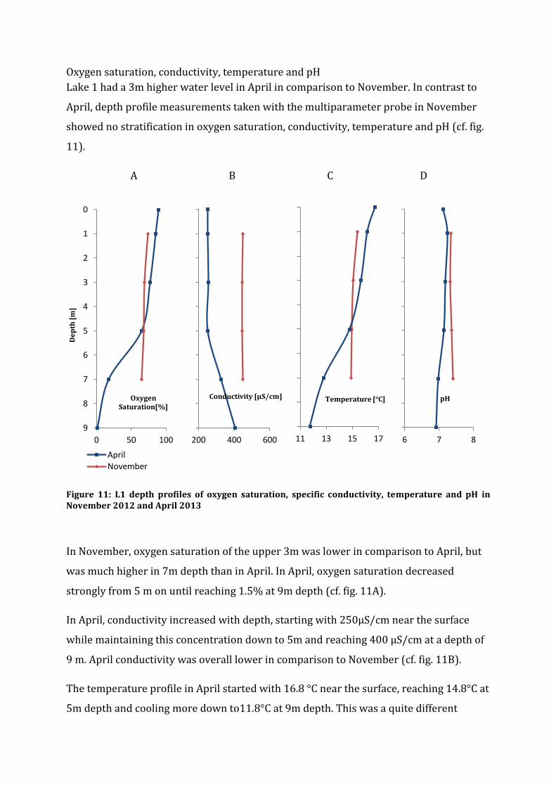
Oxygen saturation, conductivity, temperature and pH ................................................... 50
3.3.2 Lake 1 Inflows ........................................................................................................................... 51
3.3.3 Lake 2 ............................................................................................................................................ 51
3.3.4 Lake 3 ............................................................................................................................................ 52
3.3.5. Lake 4 ........................................................................................................................................... 52
Ion Concentrations ........................................................................................................................ 52
Ion balances ...................................................................................................................................... 54
Oxygen saturation, conductivity, temperature and pH ................................................... 54
3.3.6 Lake 5 ............................................................................................................................................ 55
Lake water trophic state .............................................................................................................. 69
Stratification of L1 and L4 .......................................................................................................... 70
Lake water quality ......................................................................................................................... 72
Differences between lakes .......................................................................................................... 75
4.1.6 Rain water ................................................................................................................................... 75
4.1.7 Ion Balances ............................................................................................................................... 76
4.1.8 Isotopic composition of ground- and surface waters ..................................................... 76
4.2. Interactions between ground- and surface water .............................................................. 78
4.2.1 Groundwater leakage into lakes......................................................................................... 78
4.2.2 Lake 4 leakage into SW1........................................................................................................ 80
4.2.3 L1 leakage into S3 .................................................................................................................... 81
4.3 Water supply ...................................................................................................................................... 81
4.4. Waste water management ........................................................................................................... 83
Figure 1: Map of Iberian Peninsula with marked location of the study area. Source:
Google maps ................................................................................................................................................... 13
Figure 2: Geomorphology of the study area, the red line marks land boundary of Tamera
ecovillage. Source: Instituto Geográfico do Exésito Portugal, Carta Militar N° 545 ........... 14
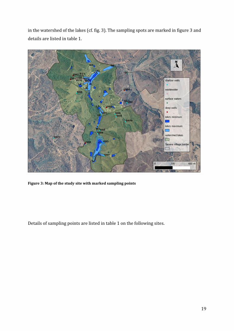
Figure 3: Map of the study site with marked sampling points ................................................... 19
Figure 4: Water tables of shallow wells 1-10 from October 2012 to November 2013. SW1
was only measured in November 2012 and April 2013 during sampling. ............................ 34
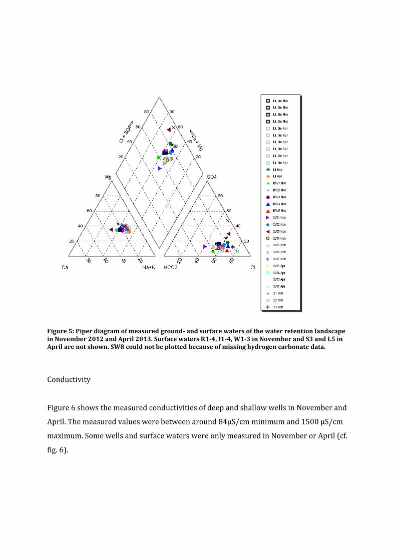
Figure 5: Piper diagram of measured ground- and surface waters of the water retention
landscape in November 2012 and April 2013. Surface waters R1-4, I1-4, W1-3 in
November and S3 and L5 in April are not shown. SW8 could not be plotted because of
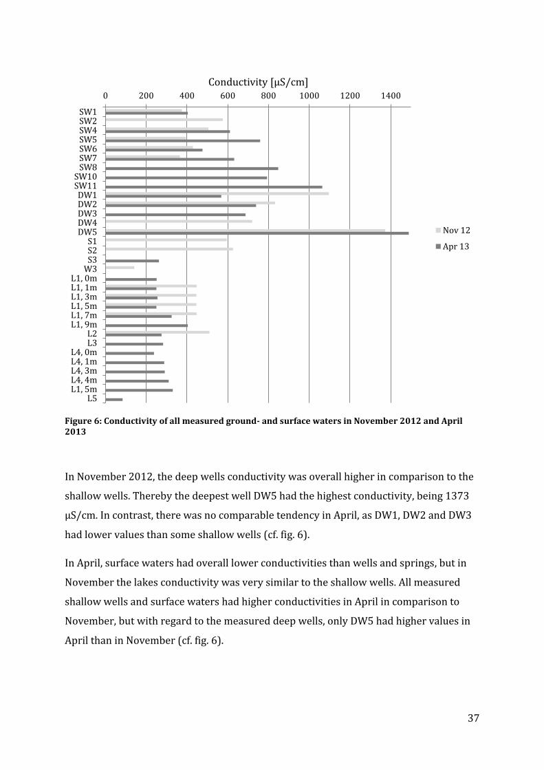
Figure 6: Conductivity of all measured ground- and surface waters in November 2012
and April 2013 ............................................................................................................................................... 37
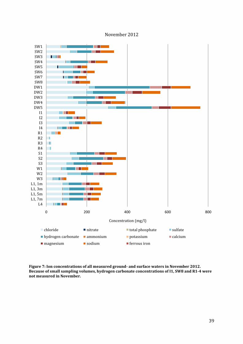
Figure 7: Ion concentrations of all measured ground- and surface waters in November
2012. Because of small sampling volumes, hydrogen carbonate concentrations of I1,
SW8 and R1-4 were not measured in November. ............................................................................ 39
Figure 8: Ion concentrations of all measured ground- and surface waters in April 2013 40
Figure 9: Depth profiles of measured ortho and total phosphate concentrations of L1 in
November 2012 and April 2013 ............................................................................................................. 48
Figure 10: Depth profiles of measured Nitrate and Ammonium concentrations of L1 in
November 2012 and April 2013 ............................................................................................................. 49
Figure 11: L1 depth profiles of oxygen saturation, specific conductivity, temperature and
pH in November 2012 and April 2013 ................................................................................................. 50
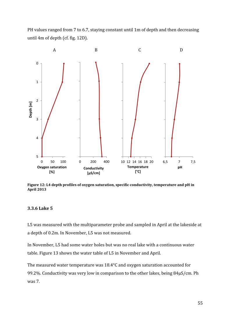
Figure 12: L4 depth profiles of oxygen saturation, specific conductivity, temperature and
pH in April 2013 ............................................................................................................................................ 55
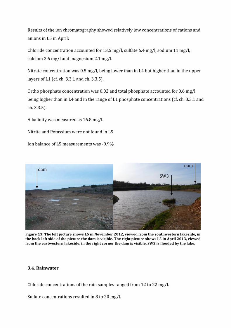
Figure 13: The left picture shows L5 in November 2012, viewed from the southwestern
lakeside, in the back left side of the picture the dam is visible. The right picture shows L5
in April 2013, viewed from the eastwestern lakeside, in the right corner the dam is
visible. SW3 is flooded by the lake. ........................................................................................................ 56
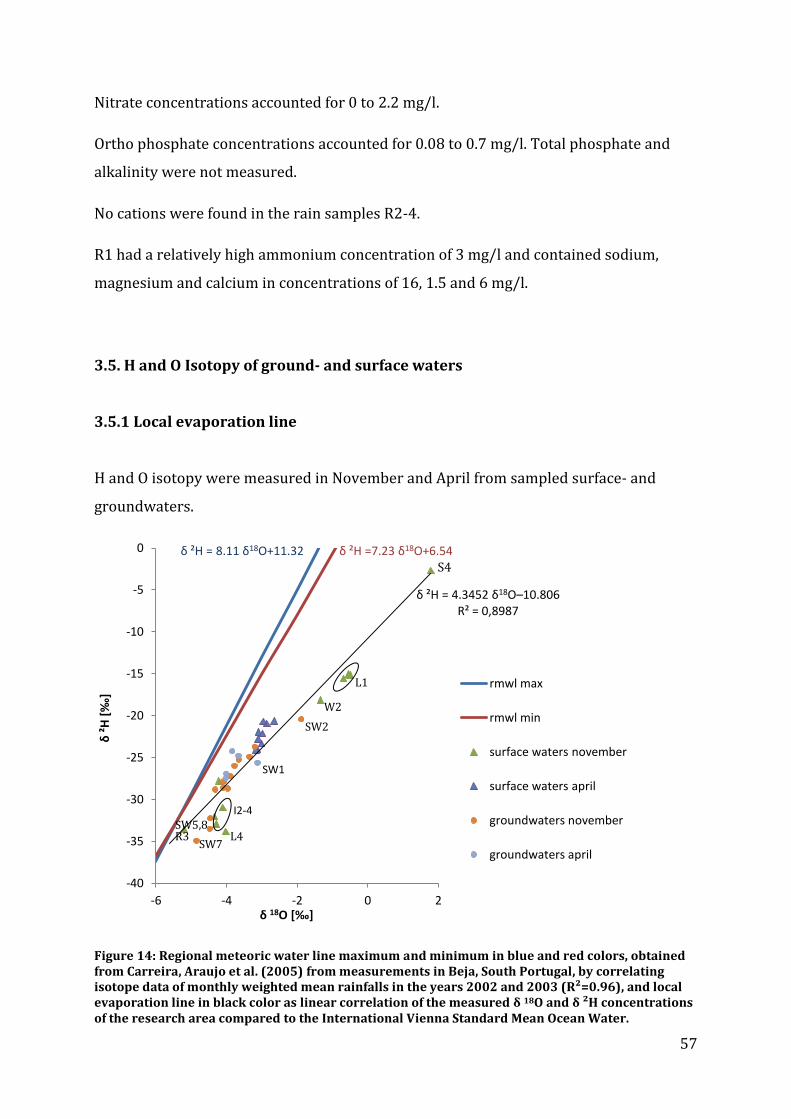
Figure 14: Regional meteoric water line maximum and minimum in blue and red colors,
obtained from Carreira, Araujo et al. (2005) from measurements in Beja, South Portugal,
by correlating isotope data of monthly weighted mean rainfalls in the years 2002 and
2003 (R²=0.96), and local evaporation line in black color as linear correlation of the
measured δ 18O and δ ²H concentrations of the research area compared to the
International Vienna Standard Mean Ocean Water. ....................................................................... 57
Figure 15: L1 depth profiles of δ 18O and δ ²H values, as compared to International
Vienna Standard Mean Ocean Water, measured in November 2012 and April 2013 ....... 59
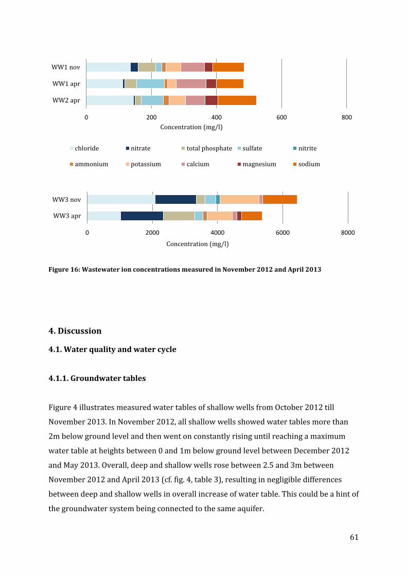
Figure 16: Wastewater ion concentrations measured in November 2012 and April 2013
Table 4: Conductivity correlation coefficients (R²) for linear correlation of the respective
cations and anions with conductivity, calculated for November 2012 and April 2013
samples from all measured deep and shallow wells. ..................................................................... 38
Table 5: SW1 and L4 δ 18O and δ ²H values, as compared to international Vienna
Standard Mean Ocean Water, measured in November 2012 and April 2013. Standard
deviation of δ 18O analysis is ±0.15‰, standard deviation of δ ²H is ±1‰. ......................... 60
Table 6: List of sampling data for temperature, conductivity, dissolved oxygen (DO) and
pH of ground-and surface waters in November 2012....................................................................... 3
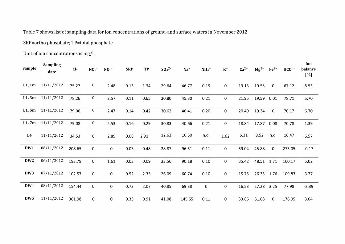
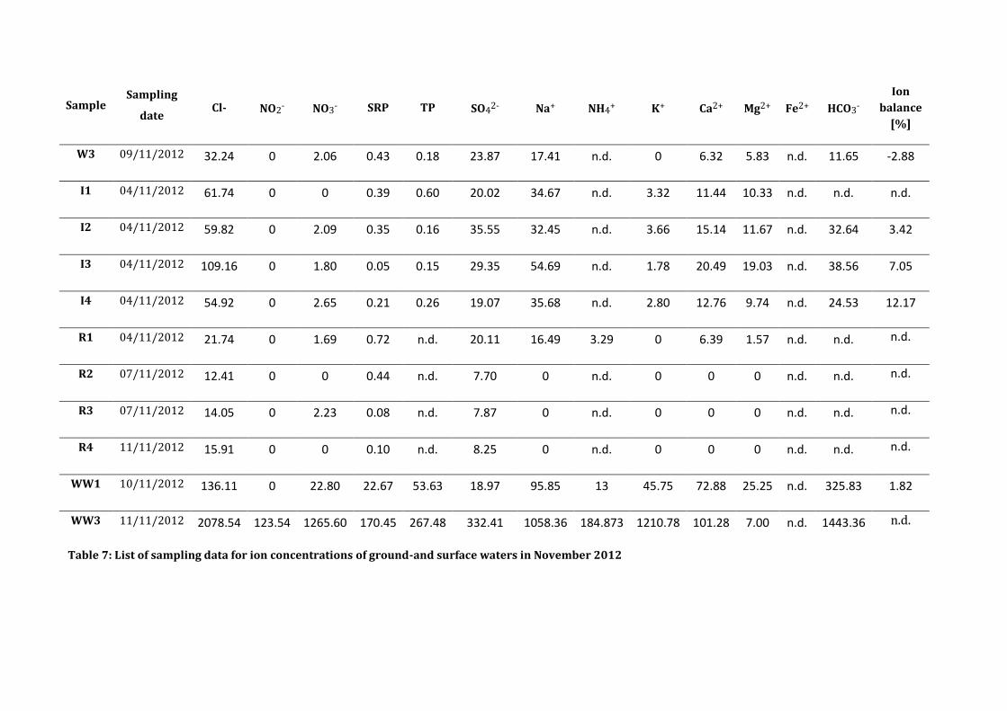
Table 7: List of sampling data for ion concentrations of ground-and surface waters in
November 2012 ............................................................................................................................................... 6
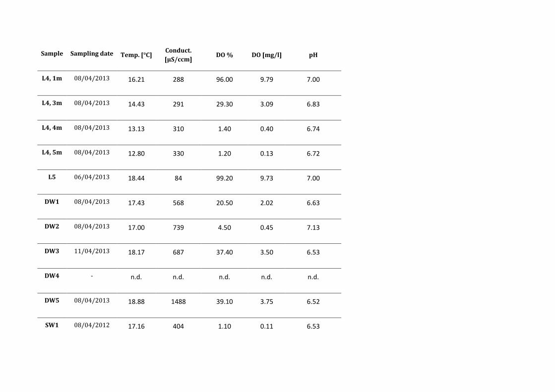
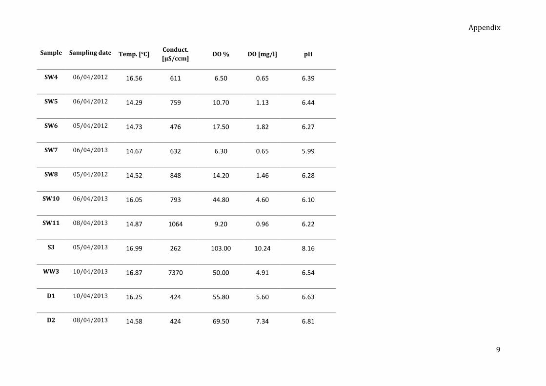
Table 8: list of sampling data for temperature, conductivity, dissolved oxygen (DO) and
pH of ground-and surface waters in April 2013 ............................................................................... 10
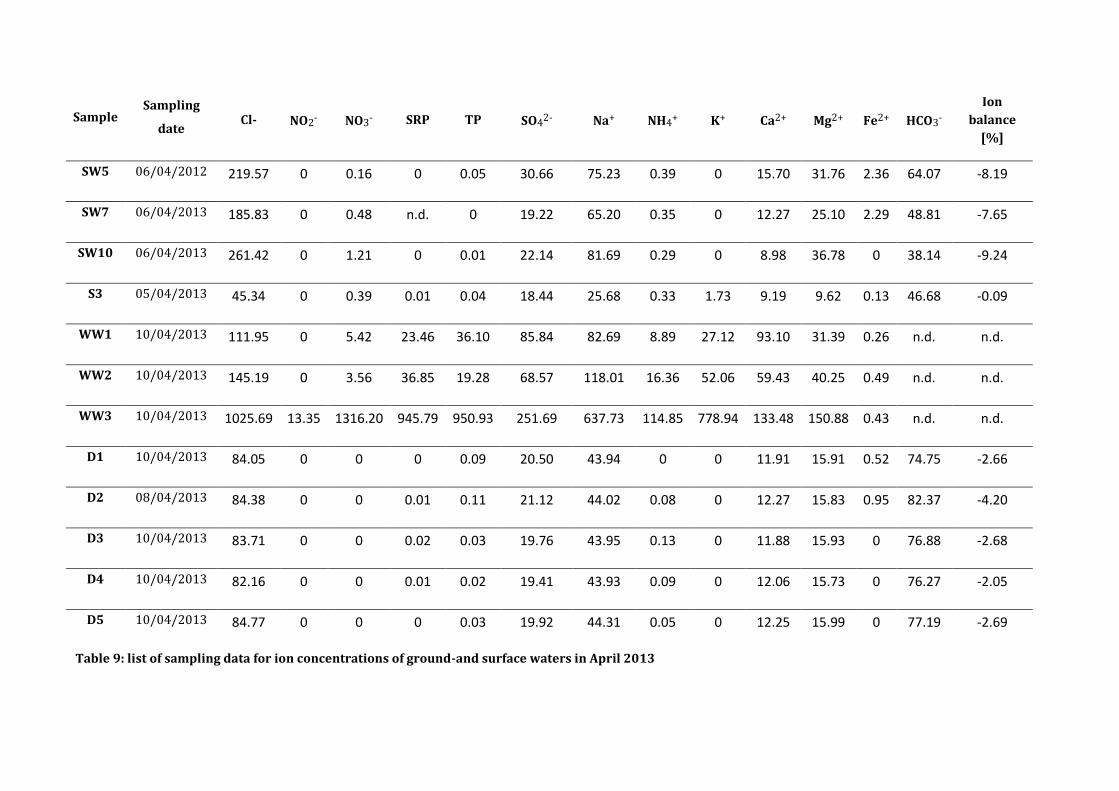
Table 9: list of sampling data for ion concentrations of ground-and surface waters in
April 2013 ........................................................................................................................................................ 12
Abbreviations
cf. compare
ch. chapter
cm centimeter
e.g. for example
fig. figure
g grams
km kilometers
l liters
m meters
mamsl meters above means sea level
mbgl meters below ground level
mg milligrams
µg micrograms
ml milliliters
mm millimeters
µS microsiemens
n.d. no data
VISMOV Vienna Standard Mean Ocean Water
GISP Greenland Ice Sheet Precipitation
SLAP Standard Light Antarctic Precipitation
11
1. Introduction
Water is a critical natural resource and its availability affects social, economic and
ecological sustainability. For humans and ecosystems water quality is as important as
water quantity (UNESCO 2012).
Many ecosystem services are derived directly from water and agricultural activities
especially in semi-arid and arid climate zones depend on the availability of fresh water
(UNESCO 2012).
The use of solely groundwater or in conjunction with surface water is of vital
importance in these zones in order to alleviate the effects of drought. But aquifer
recharge in semi-arid and arid zones is lower than in wet areas, because of low and
uneven temporally distributed precipitation (Estrela, Marcuello et al. 1996).
Groundwater abstraction rates for agricultural purposes have tripled worldwide over
the past 50 years and withdrawals in many basins are exceeding the recharge rates and
thus cannot be considered to be sustainable (UNESCO 2012).
As consequence of groundwater over-exploitation significant losses of habitat and
biodiversity were observed as well as impacts on the ecological integrity of streams and
wetlands (Ribeiro and daCunha 2010).
Furthermore, climate change causes major threats to global water supply such as
instability and degradation of freshwater reservoirs. Adaptation measures to extreme
weather events and increasing hydrological variability include surface and groundwater
storage in constructed reservoirs, wetlands and soil (UNESCO 2012).
In the case of Portugal, climate change contributes to an increase of water scarcity in the
south Portuguese semi-arid regions Alentejo and Algarve (Cunha, Ribeiro et al. 2006).
These regions are characterized by irregular water resources and a climate with very
hot and dry summers and cold and sometimes rainy winters. Rainfall is concentrated in
a short period of time during the wet season from November to February with irregular
cycles as periods of drought can last for three or more consecutive years (EEA 2010).
Construction of large reservoirs such as the Alqueva dam located in Alentejo region,
whose reservoir is considered to be Europe's largest artificial lake, provide fresh water
supply for agricultural, urban and industrial areas of the region, even during times of
prolonged drought (EEA 2010).
But large dam construction in water deficient areas is often controversial. Apart from
providing water storage, economical benefits and renewable energy, the flooding caused
by large dams causes disruptions in the local ecosystems (Santos, Pedroso et al. 2008).
Among them are deforestation, habitat loss and fragmentation, decline in distribution
ranges of wild animal species, lower freshwater flows downstream and thus intrusion of
saline waters into previously freshwater locations (Domingues, Sobrino et al. 2007,
Santos, Pedroso et al. 2008, Pereira and Figueiredo 2009).
Hence, water storage in soils and wetlands as well as small reservoirs for rainwater
harvesting seem to be more appropriate. Rainwater harvesting, which is broadly defined
as the collection and storage of surface runoff, has been neglected in agricultural water
supply even of a long history in traditional water supply for agricultural purposes
(Wisser, Frolking et al. 2010).
Especially the significance of rainwater harvesting in small reservoirs has been
underlined by several studies in semi-arid zones (Smith, Renwick et al. 2002, Liebe, van
de Giesen et al. 2005, Wisser, Frolking et al. 2010).
Water storage in soils of the Alentejo region seems to be rather low, as soils of the
region, derived from schist or granite, are mainly characterised bv scarcity in organic
matter, thinness and low water storage capacity (Correia 1993). Additionally, soil
erosion as a result of deforestation, agricultural mechanization and often very strong
rainfall events, contribute to low water absorption by soils of the region.
Besides the described challenges, land degradation and rural depopulation make
sustainable development of Alentejo region difficult, especially with regard to
agriculture and land management (Correia 1993). These developments seem to be
connected to increasing weather extremes and water scarcity of surface and
groundwater during the dry period (Correia 1993, EEA 2010).
To foster land and soil regeneration, various small reservoirs have been built since 2007
on the area of Tamera ecovillage, which is located in southwestern Alentejo. Rainwater
harvesting by small reservoirs enables agricultural production and local water supply
(Holzer 2012). This so called water retention landscape was assumed to raise
groundwater recharge rates by reservoir leakage into aquifers and thus to foster
reforestation and land regeneration, as previous attempts of deforestation failed due to
poor soils and dryness (Holzer 2012).
13
Study area
This study was conducted in the area of Tamera ecovillage in southwest Alentejo (cf. fig.
1), measuring 140 km² and located at Monte do Cerro which is part of the parish
Reliquias, in the Portuguese municipality of Odemira. GPS data is: 37°42´54” North,
8°30´57” West.
Figure 1: Map of Iberian Peninsula with marked location of the study area. Source: Google maps
The semi-arid climate of the area is characterized by long dry summers, where
temperatures often attain 30-4O°C, sometimes over 40°C. Annual precipitation is
concentrated in the wet period from September to April and averages about 600 mm,
but can reach between 400 and 1200mm. Precipitation during the wet season is
irregularly distributed and shows great annual fluctuations (Correia 1993). Very high
values of potential evapotranspiration, surpassing 1000 mm, mainly occur during the
period from July to September (Chambel and Almeida 1998).
Average groundwater recharge accounts for around 2-5% of annual precipitation
(Ribeiro and daCunha 2010).
Geomorphological structures of the region are extensive flat areas with some residual
relief. The study area lies between 130 and 200 mamsl in a small valley surrounded by
hills of about 200 mamsl height and other valleys (cf. fig. 2), leading into a greater valley
with a small stream. The valley of the study site is oriented south-north and opens at the
northern end (cf. fig. 2).
Figure 2: Geomorphology of the study area, the red line marks land boundary of Tamera ecovillage. Source: Instituto Geográfico do Exésito Portugal, Carta Militar N° 545
15
Rocks of the region are part of the most recent sediments of the South Portuguese Zone,
a main geostructural domain of the Iberian Peninsula Precambrian and Paleozoic Shield,
derived from sedimentary and volcanic rocks and compressed during the Hercynian
Orogeny (Chambel and Almeida 1998). The South Portuguese Zone consists mainly of
metamorphic rocks such as shales, schists, phylites, greywackes, quartzites and acid and
basic metavolcanic rocks. Rocks are formed by quartz, feldspar (mainly calcium
feldspars), micas and clay minerals, particularly caolinite, illite and chlorite. In some
parts of the region, carbonates, pyrite and haematite occur in smaller percentages
(Pinho, Duarte et al. 2007).
Outcropping shales of the study area are part of the Mira formation, a subdivision of the
Baixo Alentejo Flysch Group, which is one of the domains of the South Portuguese Zone,
consisting of deepwater turbiditic sediments more than 5 km thick (Fernandes, Orge et
al. 2008). Age of Mira formation is late Viséan to early Bashkirian in the Carboniferous
respective 345 to 315 million years (Pereira, Matos et al. 2007)
Hard rock aquifers with low permeabilities characterize the hydrogeology of the region,
resulting in low aquifer yields, except zones of high fracturing (Chambel 2006).
Groundwater in the South Portuguese Zone has a deficient quality with high values of
electrical conductivity and sodium-chloride as dominant hydrogeochemical facies
(Chambel and Almeida 1998).
For the South Portuguese Zone, three aquifer systems are proposed by Chambel and
Almeida (1998): a superficial water table aquifer on a weathered and fractured zone in
the first 50 meters, followed by an intermediate aquifer with low permeability but
widely spaced vertical fractures which can function as high conductive channels. Finally,
a deeper system of highly fractured pyrite masses and rocks in the deepest zones is
proposed. However in some places only the first two systems would be present
(Chambel and Almeida 1998). Changes of the hydraulic head lead to the interaction of all
three systems so that the intermediate system acts as a channel connecting upper and
deeper system (Chambel and Almeida 1998).
Soils of the study site are heavy Luvisols in the valleys and Leptosols on the hills with pH
around 6.
The cultivated landscape in the Alentejo region is characterized by the traditional agro-
silvo-pastoral system, a dispersion of individual trees or groups of trees, associated with
animal grazing and cultivation. Occurring trees are Quercus suber, Quercus rotundifolia,
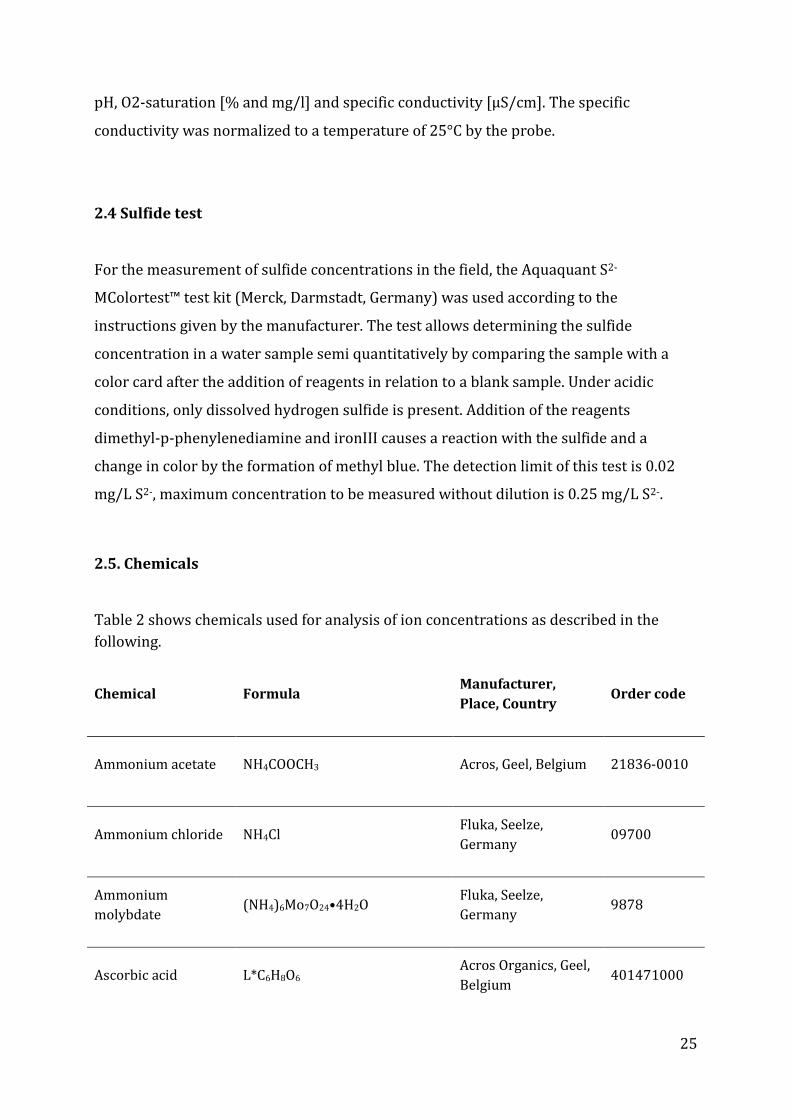
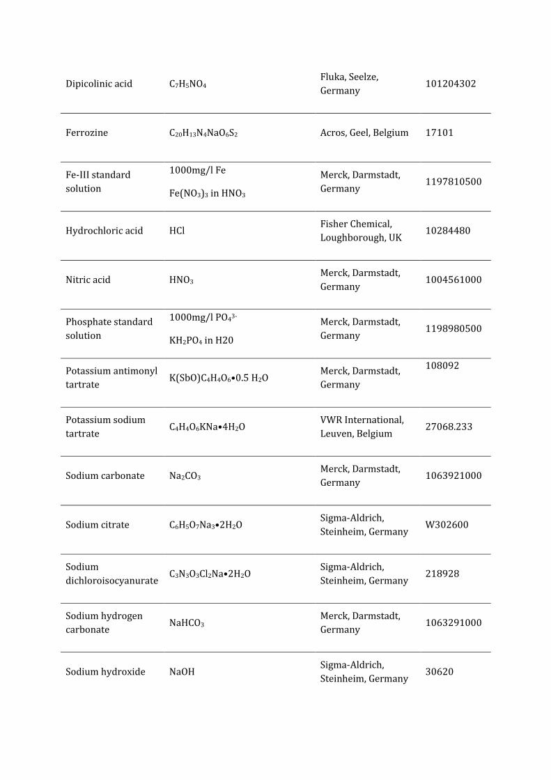
Photometric measurements were made with a photoLab 6600 UV-Vis
spectrophotometer (WTW, Weilheim, Germany), using 1cm disposable polystyrol
cuvettes and 5cm glass cuvettes.
2.6.1 Orthophosphate and total phosphate
For the determination of ortho- and total phosphate concentrations of the samples a
photometric method based on a modified version of Murphy and Riley (1962) was
applied. Briefly, ortho-phosphate and molybdate build up phosphor-molybdate
heteropolyacid under acidic conditions, while the following addition of ascorbic acid
reduces the molybdate, forming a deep blue complex that is measured with a
photometer.
Samples for the measurement of total phosphate underwent an oxidative pretreatment
to digest the biomass in the unfiltered samples. Therefore 5 ml of each sample were put
in high-pressure testing tubes with an addition of 250 μl of sodium peroxodisulfate
(5%). Afterwards, the samples were autoclaved for 2 hours at 121°C.
For the photometric measurement of orthophosphate and total phosphate the following
reagents were prepared:
Molybdate sulfuric acid:
For 50 ml, 0.035 g potassium antimonyl tartrate were dissolved in 10ml of millipore
water.
Then 1.3g ammonium molybdate were dissolved in another 10 ml of millipore water. 25
ml of a 1:1 diluted sulfuric acid were prepared in a 50 mL flask. In the following the
molybdate solution and the tartrate solution were added and then everything was
diluted to 50 ml. On the day of the analysis, a 6.25 dilution with millipore water was
prepared.
10% ascorbic acid:
1g of ascorbic acid was diluted with 10ml of millipore water. On the day of the analysis,
the solution was diluted 25 times with millipore water.
Standard series were prepared with a phosphate (PO43-) stock solution (1000mg/l).
2ml of a 1:1 mixture of ascorbic acid (10%) and molybdate sulfuric acid were mixed
with 1ml of sample or standard and filled into a 1cm plastic or 5cm glass cuvette,
according to the expected concentration. After a reaction time of 30 minutes, the
extinction was measured with a wavelength of 710 nm with the photometer. 5 to 8
standards were used to construct a calibration curve of each measurement (R2 ranged
from 0.98 to 0.99).
2.6.2 Ammonium
The measurement of NH4-N was done with a modified method after Krom (1980). The
method is based on the substitution reaction of ammonium with sodium
29
dichloroisocyanurate to chloramines. In presence of sodium nitroprusside, which acts as
a catalyst, the chloramines form blue-greenish indophenol complexes.
For the measurement four reagents were prepared:
A) Buffer solution
For 250 ml, 8.25g potassium sodium tartrate were dissolved in 125 ml millipore water,
then 6g sodium citrate were added. Finally the solution was diluted with millipore water
to 250 ml. The pH was controlled to be 5.2 and was optionally adjusted with 6N HCl.
B) Sodium salicylate solution
2.5 g sodium hydroxide were dissolved in 50 ml millipore water and then 8g of sodium
salicylate were added. Then the solution was diluted with millipore water to 100 ml.
C) Sodium nitroprusside solution
0.1 g sodium nitroprusside were dissolved in 100 ml millipore water.
Reagents B and C were mixed in the ratio of 2:1 (v:v) on the day of analysis.
D) Sodium dichlorisocyanurate solution
This solution was prepared freshly on the day of analysis. For 50ml, 0.2 g sodium
dichlorisocyanurate were dissolved in 50 ml millipore water.
Standards were prepared with ammonium chloride. For the analysis 1ml of reagent A
was given into a 1cm polystyrol cuvette and 600μl of the mixture of B and C were added.
Then 1 ml of the sample or standard was added and finally 400 μl of solution D were
given into the cuvette.
Furthermore, the cuvette was closed with a lid, shaken shortly and left in the dark. After
a reaction time of one hour the extinction was measured with a wavelength of 660 nm. 6
standards were used to construct a calibration curve of each measurement (R2 was
0.99).
2.6.3 Ferrous iron
The determination method of ferrous iron was based on a modified version of Stookey
(1970). It relies on the principle that ferrous iron reacts with ferrozine in a 1:3 ratio:
three molecules of ferrozine form a purple, water soluble complex with one Fe2+-ion at
pH 4 to 9.
For the quantification the following reagents were prepared:
Ferrozine solution:
250 g (50% w/v) ammonium acetate and 0.5 g (0.1% w/v) ferrozine were dissolved in
500 ml millipore water. The solution was stored in the dark at 4°C.
10% ascorbic acid:
10g of ascorbic acid were dissolved in 100 ml millipore water. This solution was only
used for the preparation of the standards.
50% sulfuric acid:
A 1:1 (v/v) dilution of sulfuric acid with millipore water was prepared.
For the preparation of the standards, a Fe-III standard solution (1000 mg/l) was used
together with the sulfuric acid and ascorbic acid solutions.
0.5 ml of the prepared sulfuric acid with the respective amount of stock solution were
put into a flask, then 1ml of ascorbic acid was added to reduce iron-III to iron-II and
finally the solution was diluted with millipore water to a volume of 50ml.
For measuring of ferrous iron concentrations in the samples 1 ml of ferrozine reagent
and 1 ml of sample or standard were filled into a 1 cm disposable polystyrol cuvette. The
samples were kept dark and after a reaction time of 10 minutes the extinction was
31
measured with a wavelength of 562 nm. 8 standards were used to construct a
calibration curve of each measurement (R2 was 0.99).
2.7 Titrimetric determination of alkalinity
For the determination of alkalinity, 50 ml of the water sample were titrated with 0.05 N
HCl until reaching a pH of 4.2. Meanwhile the sample was mixed continuously with the
acid by a magnetic stirrer and the pH was controlled with a pH electrode.
The titrated volume of acid was used to calculate the corresponding alkalinity by using
equation 1.
Calk is the alkalinity in mmol/l, CHCl represents the concentration of the acid in mol/l, VHCL is the
volume of the titrated HCL and Vsample the volume of the sample, the unit of the volumes is ml.
At a pH of 4.2, HCO3- is the most dominant species of the carbonates, so the
concentration of HCO3-was assumed to equal the alkalinity (Neal 1988).
2.8 Ion Chromatography and calculation of the ion balance
For the determination of various cation and anion concentrations in the water samples
the ion chromatograph 883 Basic IC plus (Metrohm, Filderstadt, Germany) was used,
connected to an 863 Compact IC Autosampler (Metrohm, Filderstadt, Germany). The
columns Metrosept C4-250/4.0 and Supp 4-250/4.0 (Metrohm, Filderstadt, Germany)
were used for cation and anion analysis.
For the measurement of the cations magnesium, calcium, potassium and sodium a
solution of 1.7 mmol/l nitric acid and 0.7 mmol/l dipicolinic acid was used as an eluent.
For the measurement of the anions sulfate, nitrate, nitrite and chloride, the eluent
consisted of 1 mmol/l sodium carbonate and 4 mmol/l sodium hydrogen carbonate.
Samples with sulfide content were degassed with nitrogen before measurement. The
waste water samples were diluted with millipore water by factors between 10 and 20
for the ion chromatographic analysis.
To estimate the quality of the measured ion concentrations, an ion balance was
calculated for every sample. Therefore all measured cation and anion concentrations
were transformed into normal concentrations by applying equation 2.
Then the normal concentrations were summed up for the ion balance with the use of
equation 3.
Ion balances up to ±5% were regarded as a tolerable quality (Hölting and Coldewey
2013).
2.9 Isotope analysis
2.9.1 Measurement of δ18O isotopy
10 ml screwcap exetainer vials were filled with a gas mixture of 0.3% CO2 in helium with
a purity of 99.996% and then closed with a membrane cap liner.
In the following approximately 500μl of the sample were injected with a syringe through
the membrane into the vial. In order to allow 18O equilibration between CO2 and H2O,
samples were kept closed for 24 hours. Afterwards, the samples were quantified
through injection with a Gas Bench II (Finnigan-Thermo Fisher Scientific, Schwerte,
Germany) in a MAT 252 mass spectrometer (Finnigan-Thermo Fisher Scientific,
Schwerte, Germany) by using helium as carrier gas and the continuous flow method.
Standard deviation of this analysis was about 0.15‰.
33
2.9.2 Measurement of ²H isotopy
During the analysis the water samples were reduced by chromium to H2 in an H-Device
(Thermo Fisher Scientific, Schwerte, Germany) at 800°C. The H2 was then quantified in
the mass spectrometer MAT 252 (Thermo Fisher Scientific, Schwerte, Germany) with
the dual-inlet method without any carrier gas.
The repeatability of this method is about ±1‰.
Calibration was done with the three international standards of VSMOV (δ18O=0‰,
δ²H=0‰), GISP (δ18O =-24.75‰, δ²H =-189.9‰, relative to VSMOV) and SLAP
(δ 18O =-55.5‰, δ²H =-428‰, relative to VSMOV).
3. Results
3.1. Groundwater
3.1.1. Groundwater tables
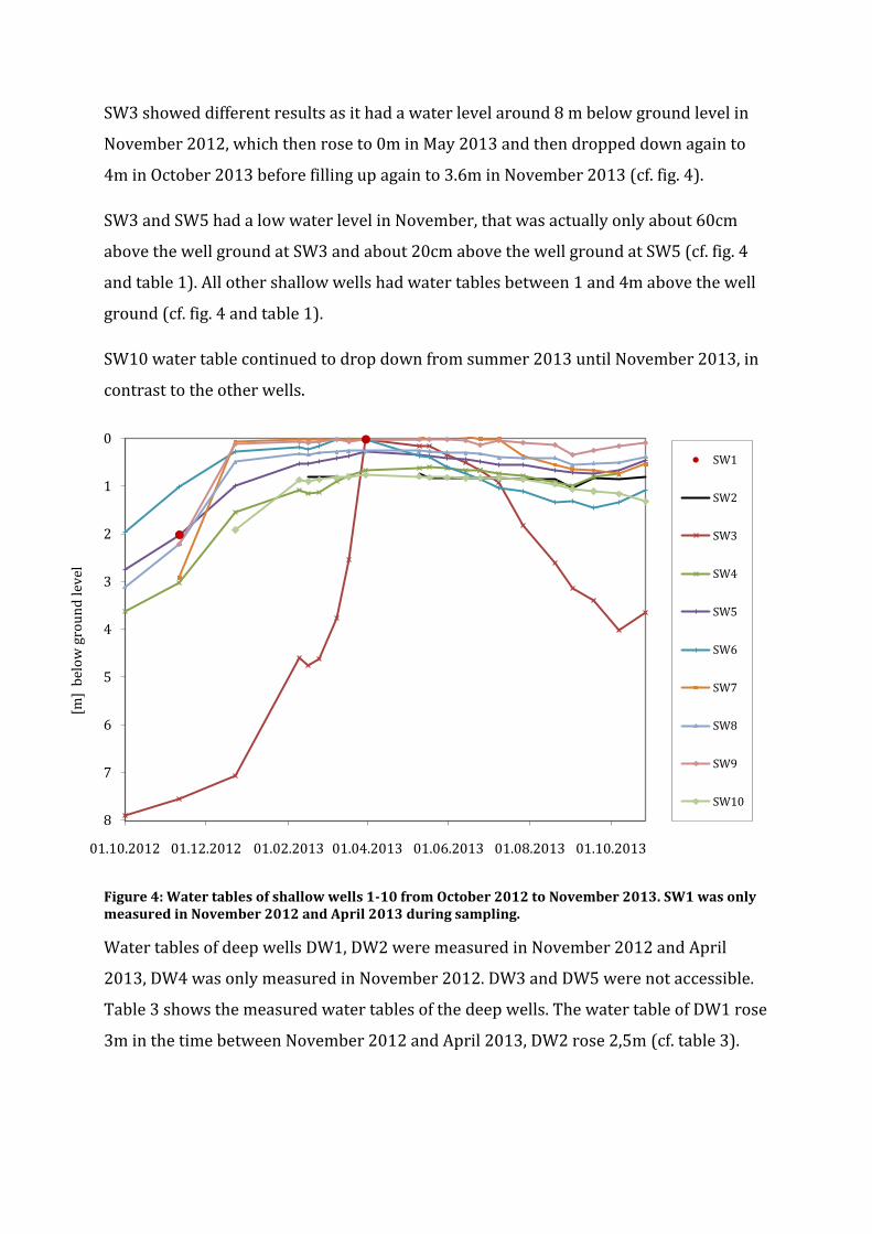
Figure 4 shows the measured water tables of shallow wells from October 2012 till
November 2013. In November 2012, water tables of all shallow wells were more than
2m below ground level and were constantly rising until reaching a maximum water table
at heights between 0 and 1m below ground level in the time between December 2012
and May 2013.
All measured shallow wells except SW3 and SW6 stayed at their maximum height for
around two months between March and June 2012 and then slowly dropped down to
water levels between 0 and 1.5m below ground level in September 2013, before filling
up again in November 2013 to heights between 0 and 1 m below ground level (cf. fig. 4).
SW1, which was measured only in November 2012 and April 2013 during sampling,
showed a water table of 2m below ground in November and 0m below ground level in
April. In April, the grassland area around SW1 was swampy and at some locations
around 10cm of water had risen out of the ground on the soil surface.
SW3 showed different results as it had a water level around 8 m below ground level in
November 2012, which then rose to 0m in May 2013 and then dropped down again to
4m in October 2013 before filling up again to 3.6m in November 2013 (cf. fig. 4).
SW3 and SW5 had a low water level in November, that was actually only about 60cm
above the well ground at SW3 and about 20cm above the well ground at SW5 (cf. fig. 4
and table 1). All other shallow wells had water tables between 1 and 4m above the well
ground (cf. fig. 4 and table 1).
SW10 water table continued to drop down from summer 2013 until November 2013, in
contrast to the other wells.
Figure 4: Water tables of shallow wells 1-10 from October 2012 to November 2013. SW1 was only measured in November 2012 and April 2013 during sampling.
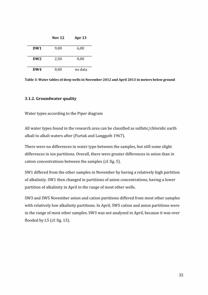
Water tables of deep wells DW1, DW2 were measured in November 2012 and April
2013, DW4 was only measured in November 2012. DW3 and DW5 were not accessible.
Table 3 shows the measured water tables of the deep wells. The water table of DW1 rose
3m in the time between November 2012 and April 2013, DW2 rose 2,5m (cf. table 3).
Table 3: Water tables of deep wells in November 2012 and April 2013 in meters below ground
3.1.2. Groundwater quality
Water types according to the Piper diagram
All water types found in the research area can be classified as sulfatic/chloridic earth
alkali to alkali waters after (Furtak and Langguth 1967).
There were no differences in water type between the samples, but still some slight
differences in ion partitions. Overall, there were greater differences in anion than in
cation concentrations between the samples (cf. fig. 5).
SW1 differed from the other samples in November by having a relatively high partition
of alkalinity. SW1 then changed in partitions of anion concentrations, having a lower
partition of alkalinity in April in the range of most other wells.
SW3 and SW5 November anion and cation partitions differed from most other samples
with relatively low alkalinity partitions. In April, SW5 cation and anion partitions were
in the range of most other samples. SW3 was not analyzed in April, because it was over
flooded by L5 (cf. fig. 13).
Figure 5: Piper diagram of measured ground- and surface waters of the water retention landscape in November 2012 and April 2013. Surface waters R1-4, I1-4, W1-3 in November and S3 and L5 in April are not shown. SW8 could not be plotted because of missing hydrogen carbonate data.
Conductivity
Figure 6 shows the measured conductivities of deep and shallow wells in November and
April. The measured values were between around 84µS/cm minimum and 1500 µS/cm
maximum. Some wells and surface waters were only measured in November or April (cf.
fig. 6).
37
Figure 6: Conductivity of all measured ground- and surface waters in November 2012 and April 2013
In November 2012, the deep wells conductivity was overall higher in comparison to the
shallow wells. Thereby the deepest well DW5 had the highest conductivity, being 1373
µS/cm. In contrast, there was no comparable tendency in April, as DW1, DW2 and DW3
had lower values than some shallow wells (cf. fig. 6).
In April, surface waters had overall lower conductivities than wells and springs, but in
November the lakes conductivity was very similar to the shallow wells. All measured
shallow wells and surface waters had higher conductivities in April in comparison to
November, but with regard to the measured deep wells, only DW5 had higher values in
April than in November (cf. fig. 6).
0 200 400 600 800 1000 1200 1400
SW1 SW2 SW4 SW5 SW6 SW7 SW8
SW10 SW11 DW1 DW2 DW3 DW4 DW5
S1 S2 S3
W3 L1, 0m L1, 1m L1, 3m L1, 5m L1, 7m L1, 9m
L2 L3
L4, 0m L4, 1m L4, 3m L4, 4m L1, 5m
L5
Conductivity [µS/cm]
Nov 12
Apr 13
Assuming one aquifer system for all wells because of the described similarities of ion
partitions shown in the Piper diagram, ions were correlated with conductivity to get an
overview of the whole areas hydrogeological situation. Overall, there was a strong
correlation with a linear relationship for all wells in November and April between
conductivity and chloride concentrations, sodium concentrations and conductivity, as
well as for magnesium and conductivity (cf. table 4). Higher ion concentrations
correlated with higher conductivities. No clear pattern was found for calcium and
hydrogen carbonate concentrations, and no correlation for sulfate concentrations and
conductivity.
Cl- Na+ Mg2+ Ca2+ HCO3- SO43-
April 2013 0.94 0.94 0.93 0.07 0.24 0.3
November 2012 0.97 0.97 0.98 0.63 0.6 0
Table 4: Conductivity correlation coefficients (R²) for linear correlation of the respective cations and anions with conductivity, calculated for November 2012 and April 2013 samples from all measured deep and shallow wells.
Ion concentrations
Figure 7 and 8 show the measured ion concentrations of all ground- and surface waters
in November and April. Groundwaters differed from surface waters in both months in
ion concentrations. Details are described in the following and can be found in the
appendix.
39
Figure 7: Ion concentrations of all measured ground- and surface waters in November 2012. Because of small sampling volumes, hydrogen carbonate concentrations of I1, SW8 and R1-4 were not measured in November.
Nitrate concentration was 0.5 mg/l, being lower than in L4 but higher than in the upper
layers of L1 (cf. ch. 3.3.1 and ch. 3.3.5).
Ortho phosphate concentration was 0.02 and total phosphate accounted for 0.6 mg/l,
being higher than in L4 and in the range of L1 phosphate concentrations (cf. ch. 3.3.1 and
ch. 3.3.5).
Alkalinity was measured as 16.8 mg/l.
Nitrite and Potassium were not found in L5.
Ion balance of L5 measurements was -0.9%
3.4. Rainwater
Chloride concentrations of the rain samples ranged from 12 to 22 mg/l.
Sulfate concentrations resulted in 8 to 20 mg/l.
dam dam
SW3
Figure 13: The left picture shows L5 in November 2012, viewed from the southwestern lakeside, in the back left side of the picture the dam is visible. The right picture shows L5 in April 2013, viewed from the eastwestern lakeside, in the right corner the dam is visible. SW3 is flooded by the lake.
57
Nitrate concentrations accounted for 0 to 2.2 mg/l.
Ortho phosphate concentrations accounted for 0.08 to 0.7 mg/l. Total phosphate and
alkalinity were not measured.
No cations were found in the rain samples R2-4.
R1 had a relatively high ammonium concentration of 3 mg/l and contained sodium,
magnesium and calcium in concentrations of 16, 1.5 and 6 mg/l.
3.5. H and O Isotopy of ground- and surface waters
3.5.1 Local evaporation line
H and O isotopy were measured in November and April from sampled surface- and
groundwaters.
Figure 14: Regional meteoric water line maximum and minimum in blue and red colors, obtained from Carreira, Araujo et al. (2005) from measurements in Beja, South Portugal, by correlating isotope data of monthly weighted mean rainfalls in the years 2002 and 2003 (R²=0.96), and local evaporation line in black color as linear correlation of the measured δ 18O and δ ²H concentrations of the research area compared to the International Vienna Standard Mean Ocean Water.
δ ²H = 4.3452 δ18O–10.806 R² = 0,8987
-40
-35
-30
-25
-20
-15
-10
-5
0
-6 -4 -2 0 2
δ ²
H [
‰]
δ 18O [‰]
rmwl max
rmwl min
surface waters november
surface waters april
groundwaters november
groundwaters april
δ ²H =7.23 δ18O+6.54 δ ²H = 8.11 δ18O+11.32
I2-4
SW1
L1
W2
SW7 SW5,8
SW2
L4 R3
S4
Figure 14 shows the local evaporation line in comparison to the regional meteoric water
line obtained from Carreira, Araujo et al. (2005), where the deviation of the local
evaporation line shows an existing influence of evaporation on the waters in the
research area. November surface waters S4, L1 and W2 showed the strongest influence
by evaporation, having the heaviest isotopies. In contrast, November samples SW5, 7
and 8 as well as I2-4 and L4 had the lightest isotopies and were therefore the nearest
samples to the rainwater isotopie of R3. April samples differed clearly between surface-
and ground waters, where ground waters had lighter isotopies than surface waters (cf.
fig. 14).
According to Gibson, Edwards et al. (1993) mean annual rain isotopic compositon of the
study site was calculated to be -5.877 ‰ δ 18O and -36.342 ‰ δ ²H, marking the
intersection of regional meteoric water line and local evaporation line.
3.5.2 Isotopic depth profile of L1
L1 isotopy was heavier in November than in April (cf. fig. 15). November δ 18O and δ ²H
values did not show stratification in lake water isotopy. In April, a clear stratification
was detectable, as in depth of 7 and 9m δ 18O and δ ²H values were significantly heavier
in comparison to the upper water layers of L1 (cf. fig. 15).
59
Figure 15: L1 depth profiles of δ 18O and δ ²H values, as compared to International Vienna Standard Mean Ocean Water, measured in November 2012 and April 2013
3.5.3 Isotopy of SW1 and L4
To detect possible influences of L4 on SW1, isotopic data of both waters were measured.
Oxygen and Hydrogen isotopies of SW1 and L4 differed in November with a difference of
0.83‰ for δ 18O and 10.07‰ for δ ²H, where SW1 isotopy was overall heavier than L4
isotopy. In April, the opposite was the case and the differences were relatively small,
being 0.14‰ for δ 18O and 3.51‰ for δ ²H (cf. table 5).
-3.11
-3.13
-3.17
-2.86
-2.65
-0.69
-0.50
-0.55
0
1
2
3
4
5
6
7
8
9
10
-4 -3 -2 -1 0
de
pth
[m
]
δ 18O [‰]
-22.78
-24.04
-24.12
-20.94
-20.66
-15.56
-15.15
-15.01
-25 -20 -15 -10
δ ²H [‰]
April
November
δ 18O [‰] δ ²H [‰]
Nov 2012 Apr 2013 Nov2012 Apr 2013
SW1 -3,20 -3,12 -23,73 -25,62
L4 -4,03 -2,98 -33,80 -22,11
Table 5: SW1 and L4 δ 18O and δ ²H values, as compared to international Vienna Standard Mean Ocean Water, measured in November 2012 and April 2013. Standard deviation of δ 18O analysis is ±0.15‰, standard deviation of δ ²H is ±1‰.
3.6. Wastewaters
WW1 and WW3 were measured in November 2012 and April 2013, WW2 was measured
in April only. Figure 16 shows ion concentrations of the wastewaters. WW3 had ion
concentrations around ten times higher than WW1 and WW2, with higher
concentrations in November than in April. Ion concentrations of WW2 in April were
lower than WW1 concentrations. WW1 had almost constant ion concentrations in both
months, but less nitrate, total phosphate, ammonium and potassium in April than in
November (cf. fig. 16).
Total nitrogen concentrations of WW1 being 15.2 mg/l in November and 8.1 mg/l in
April did not exceed EU maximum concentrations for urban waste water in sensitive
areas of 15mg/l total nitrogen (EU 1991) in both months. Total phosphorus values
exceeded EU maximum concentration for urban waste water of 2mg/l total phosphorus
for sensitive areas in both months (EU 1991), being 12.7mg/l in November and 8.5 mg/l
in April.
61
Figure 16: Wastewater ion concentrations measured in November 2012 and April 2013
4. Discussion
4.1. Water quality and water cycle
4.1.1. Groundwater tables
Figure 4 illustrates measured water tables of shallow wells from October 2012 till
November 2013. In November 2012, all shallow wells showed water tables more than
2m below ground level and then went on constantly rising until reaching a maximum
water table at heights between 0 and 1m below ground level between December 2012
and May 2013. Overall, deep and shallow wells rose between 2.5 and 3m between
November 2012 and April 2013 (cf. fig. 4, table 3), resulting in negligible differences
between deep and shallow wells in overall increase of water table. This could be a hint of
the groundwater system being connected to the same aquifer.
0 200 400 600 800
WW1 nov
WW1 apr
WW2 apr
Concentration (mg/l)
chloride nitrate total phosphate sulfate nitrite
ammonium potassium calcium magnesium sodium
0 2000 4000 6000 8000
WW3 nov
WW3 apr
Concentration (mg/l)
The rise in water tables in November 2012 indicates the beginning of the rainfall period
and shows the immediate reaction of the vadose zone to the precipitation. In 2012, the
first rain of the season was observed at 3rd of November. On 11th of November, water
tables of all shallow wells (SW3, 4, 5, 6, 8) had already risen up for at least 30cm (cf. fig.
4). Thus, the vadose zone is assumed to be highly permeable, which might be due to rock
fractionations and quartz veins in the upper weathered and fractured zone of the
topmost geologic layer (Chambel and Almeida 1998).
Most wells stayed at their maximum water table for around two months between March
and May 2012 and then slowly dropped to a water level between 0 and 1.5m below
ground level in September 2013. In November 2013 water tables filled up again
reaching 0 to 1 m below ground level (cf. fig. 4). The rise of water tables in November
2013 indicates the beginning of the rainfall period in winter 2013/14. The dropdown in
summer may be a result of evaporation and probably underground runoff through the
vadose zone. Especially in the swampy areas of the valley evaporation might have had
great impact on water tables as well as on salt accumulation in the soil (Chambel and
Almeida 1998).
The rising and falling of the shallow wells reflect weather conditions throughout 2013,
as water tables reached their minimum and maximum in times with longest dry spell
and most rainfalls, August and March, respectively (Weather Station Beja 2013).
This shows that water tables of all shallow wells are reacting almost simultaneously to
the weather conditions. However shallow wells differed in maximum water tables as
well as in rising and falling velocities of the water tables (cf. fig. 4). This indicates
varying hydrogeological situations of the single wells, probably caused by their
geographic locations. Furthermore, vegetation covers seem to have great impact on
water tables as watersheds of SW3, SW7 and SW6 with no or low tree covers (cf. table
1), showed a faster decline of water tables compared to other shallow wells with
vegetation covers like SW8 and SW9 (cf. fig. 4 and table 1). Lower groundwater recharge
rates in forested areas have also been reported by Scanlon, Keese et al. (2006).
Water table of SW10 continued to drop down from summer 2013 until November 2013
(cf. fig. 4). This could be a consequence of its location at 180mamsl in a steep
63
neighboring valley (cf. table. 1), where the first winter rainfalls most probably seep fast
through the unsaturated zone into the lower parts of the landscape. Another reason
could be the forested area around SW10 preventing substantial groundwater recharge
during the beginning of the wet season, as forest cover strongly influences groundwater
recharge rates (Scanlon, Keese et al. 2006). SW7 filled up relatively quickly in November
2012 (cf. fig. 4), which underlines the assumption that wells in deforested zones of the
research area recharge and discharge more quickly.
Water tables of SW3 strongly differed from other shallow wells, with water levels
around 8 m below ground level in November 2012. In May 2013 water level rose till 0m
and dropped to 4m in October 2013, before filling up again to 3.6m in November 2013
(cf. fig. 4). As SW3 is located at the edge of the retention space of L5 (cf. table 1, fig. 13), it
can be assumed to be highly influenced by water masses accumulating during the
rainfall period in the retention area of L5. L5 was built in the year 2011, when very poor
rainfalls in winter 2011/12 were reported (Weather Station Beja 2011, Weather Station
Beja 2012). L5 filled up with noticeable water masses for the first time during winter
2012/13, during relatively high rainfalls (Weather Station Beja 2013). Therefore time
was not sufficient for accumulation of organic and anorganic sediments at the bottom of
the lake, which would substantially lower the hydraulic permeability of the retention
space (Hölting and Coldewey 2013). As L5 is located in the upper part of the valley, it
can be assumed that parts of the water masses which accumulated during the rain
period in L5 ran down over time into the valley through the vadose zone. This might
have caused water tables to fall more quickly in the area around the lake compared to
other areas of the research site. The underground runoff could explain the depression of
the SW3 water table curve in February 2013, when low rainfalls probably did not
from L5 might percolate into the valley and contribute to runoff at the end of the valley.
In April 2013, water table of L5 did not reach the level of the dam, resulting in no
significant above ground outflow of the lake in winter 2012/13 into the valley.
Furthermore, evaporation on the surface of L5 might have had a great impact on the
local water tables around the lake and thus on well 3, which might have caused the steep
decline of SW3 water tables during summer 2013 (cf. fig. 4).
In November, SW3 ion concentrations were much lower than ion concentrations of
other ground- and surface waters and similar to rainwater (cf. fig. 7). Thus no
groundwater flow into SW3 in November 2012 is assumed. Instead accumulated old rain
water in the well might have caused lower ion concentrations. In the same time L5 was
nearly empty, which means there was no possibility of inflowing water from L5 into
SW3. With rising ground- and surface water tables in the area, SW3 probably filled up
with groundwater throughout winter 2012/13 and was flooded with surface water of L5
at the end of the wet period (cf. fig. 13). Water tables equilibrated at minimum levels of
4m below ground until October 2013 (cf. fig. 4).
The rising and falling of SW3 reflects reported weather conditions much more extremely
than the water tables of the other shallow wells. Hence, SW3 seems to be affected much
more by weather extremes than the other wells of the area. With prospective rising
water tables of L5, this pattern might change in future and could be issue of further
research.
4.1.2 Water types
Water types found in the area correspond to data for the South Portuguese Zone of
Chambel and Almeida (1998), who defined sodium-chloride to be the dominant
hydrogeochemical facies. According to the obtained correlation values, sodium chloride
and magnesium concentrations are the main causes for high conductivities of
groundwaters in the area (cf. table 4).
Differences in water type of ground- and surface waters were relatively small, with the
exception of SW3 and SW5 in November (cf. fig. 5). In November both wells showed low
water tables, with 60cm and 20 cm above the well ground for SW3 and SW5,
respectively (cf. fig. 4 and table 1). SW3 had very low ion concentrations and SW5 had a
very low alkalinity in November (cf. fig. 7 and 8). Therefore both wells might have
contained considerable amounts of rainwater at that time, as rain samples had lower ion
concentrations compared to wells and there was no possible groundwater inflow into
SW5 and SW3 in November. Around 3m away from SW5, water hole W3 is located,
which had a very low conductivity and ion concentrations similar to rainwater in
65
November. The water of W3 can be assumed to be rain water accumulating in the water
hole from the road nearby. This water then might have percolated into SW5.
Thus, the analyzed ground- and lake waters might be part of one aquifer system, as the
differences in water type are relatively small and differences of SW3 and SW5 are
probably caused by high mixing ratios of rain. As DW5 is about 60m deep, it could be
part of the intermediate aquifer system proposed by Chambel and Almeida (1998),
situated from 50m of depth on. The slightly remote position of DW5 in the Piper
diagram could be a hint for this assumption. But as described by Chambel and Almeida
(1998), the upper and intermediate aquifer systems can be connected by vertical rock
fractures that lead to interaction of both systems. Therefore DW5 can be assumed to be
influenced by the upper aquifer.
4.1.3 Conductivity of wells
The pattern of deeper ground waters having higher conductivities (cf. fig. 6) matches
with the results of Chambel and Almeida (1998). According to the authors, this would be
a consequence of minerals dissolving from the genuine rocks and migration of connate
waters due to tectonic stresses, whereby deep mineralized waters would ascend mainly
through the highly fractured rocks.
The relatively high conductivities of the shallow wells in April could be a consequence of
salts originating from the subsoil and rocks, that are being dissolved by percolating rain
water and accumulate in the groundwater (Chambel and Almeida 1998). But the
percolating rain water might dilute the conductivity of deeper layers of groundwater,
due to their relatively high conductivity (cf. fig. 6). This would explain equilibrating
conductivities of deep and shallow wells in April to each other and leads to the
assumption of a less stratified aquifer in this time period.
In this context, higher conductivities might indicate lower recharge rates. As
conductivity correlates with chloride concentrations (cf. table 4), this also could be
assumed for recharge, which accords to the results of deVries, Selaolo et al. (2000). This
would mean that the intermediate aquifer zone connected to DW5 has lower recharge
rates than the upper zone connected to the shallow wells, DW1 and DW2, which had
overall lower conductivities than DW5. DW5 has a possible intersection with the
intermediate aquifer, as discussed already above. As the intermediate aquifer was
described to have low permeability (Chambel and Almeida 1998), percolating rain water
might not reach DW5 directly and thus may not dilute DW5 ion concentrations.
Additionally, Hill and Neal (1997) reported deeper groundwater levels to be controlled
by weathering kinetics and residence times rather than by flow mechanisms.
Furthermore, shallow wells seem to have much higher recharge rates than deep wells of
the research area, as chloride concentrations in shallow wells showed consistently lower
values compared to deep wells (cf. fig. 7). However, recharge rates of the single wells
seem to differ, as different increases in chloride concentrations between November
2012 and April 2013 (cf. fig. 7 and 8) were measured.
DW5 was the only deep well with a higher conductivity in April than in November (cf.
fig. 6), but DW3 and DW4 were not measured in both months. Therefore only DW1 and
DW2 can be compared with DW5 with regard to changes in conductivity. DW5 higher
conductivity in April could be influenced by the pumping, as DW5 is the only deep well
which is still being pumped for watering and filling a small pond. Pumping might suck
mineral particles into the area around the pump and prevent recharge, which then
causes higher conductivities. As DW5 can be assumed to be part of the intermediate
aquifer, the geochemical processes in the groundwater connected to DW5 might differ
from the upper aquifer system. As flow mechanisms in the intermediate and deep
aquifer are not known, this remains issue to further research.
Because of high conductivity of DW5, its water should not be used for irrigation, to
prevent possible soil salinisation (Sequeira 2010).
4.1.4 Groundwater quality
Chloride, sodium, sulfate, magnesium and calcium in the water cycle
As discussed above, chloride could be used as an indicator for groundwater recharge
and thus different increases in chloride measured in the shallow wells between
67
November and April generally could indicate different recharge rates for the aquifer
layers around the different shallow wells.
As a general trend, all shallow wells chloride, sodium and magnesium concentrations in
April were higher compared to November (cf. fig. 7 and 8). It seems that chloride,
sodium and magnesium concentrations of the shallow wells were increased by
percolating winter rainfalls, which probably transported the ions from the subsoil into
the aquifer. This matches with the observed correlations between conductivity and
chloride, sodium and magnesium concentrations, which can be assumed to be the most
dynamic ions of the system and to accumulate in the percolating rain water.
Shallow wells sulfate concentrations did not change between the seasons, except at SW1
and SW5 (cf. fig. 7 and 8). The slight decline of SW1 sulfate concentration could be
explained by sulfate reduction to sulfide as a result of anoxic conditions (Miao, Brusseau
et al. 2012) caused by over flooding of the area around SW1 in April. Higher sulfate
concentrations in November 2012 in SW5 could be caused by evaporation leading to
concentration of sulfate. As SW5 had a very low water table in November 2012 (cf. fig.
4), the relation between surface and water volume in the well could trigger sulfate
concentration by evaporation. Overall, sulfate concentrations of the wells seemed to be
relatively stable throughout the seasons and only to be affected by changes in redox
conditions or evaporation.
Calcium did not seem to play a considerable role in the water cycle, as concentrations
stayed stable throughout the seasons and were relatively low (cf. fig. 7 and 8).
Thus, the main parameters indicating recharge of the aquifer system in the research
area can be characterized to be chloride, sodium and magnesium. Chloride can be
assumed to originate partly from the chloride containing rain (cf. fig. 7), furthermore
chloride, sodium and magnesium might be dissolved by percolating rain water from the
subsoil and vadose zone, where salts accumulate by evaporation through the dry season
(Chambel and Almeida 1998).
Nitrate, ammonium, phosphate and potassium
Nitrate, phosphate and potassium concentrations of the wells decreased between
November 2012 and April 2013 (cf. ch. 3.1.2). This might be a consequence of dilution by
rain water percolating into the aquifer as discussed above.
Most shallow wells contained nitrate in November and April (cf. ch. 3.1.2). Overall, the
range of nitrate concentrations in the wells was in the range of drinking water quality
(EU 1998) and very low in comparison to nitrate concentrations in agricultural regions
of southern Portugal, which can reach up to 50mg/l (Paralta, Carreira et al. 2007,
Ribeiro and daCunha 2010). SW1 contained no nitrate in both seasons, but low
concentrations of ammonium in April and low potassium concentrations in both seasons
were measured (cf. ch. 3.1.2). Ammonium and potassium concentrations were in the
range of maximum concentrations for drinking water (EU 1998). Thus influence of
agricultural systems on geochemical parameters of SW1 seems to be in an acceptable
range. Total phosphate concentrations of some shallow wells were relatively high,
reaching up to 4.5 mg/l (cf. ch. 3.1.2). This could be a consequence of the sampling
technique, which enabled sediments from the bottom of the well to enter the
groundwater sampler. Thus, total phosphate results probably do not correspond to total
phosphate concentrations of the wells, which might be much lower. Ortho phosphate
concentrations were in the range of drinking water quality (EU 1998).
Overall, agricultural effects on the groundwater concentrations of nitrate, phosphate and
potassium in the research area seem to be negligible under the current crop growing
methods.
Alkalinity
Higher alkalinities of the shallow wells in April (cf. ch. 3.1.2) could be a result of
carbonates being transported by rain percolation from the subsoil and vadose zone into
the groundwater. SW1 had a lower alkalinity in April 2013 than in November 2012 (cf.
ch. 3.1.2) and might have been influenced by the water quality of L4, as discussed in
chapter 4.2.2.
Ferrous iron
Most wells showed relatively high ferrous iron concentrations (cf. ch. 3.1.2), which
might be a result of the local geology and the generally low oxygen saturation levels of
69
the groundwaters. Ferrous iron concentrations of most wells exceeded the limit for
drinking water of 0.5 mg/l (EU 1998).
Oxygen saturation
The generally low oxygen saturation levels of the groundwaters (cf. ch. 3.1.2) might be
caused by chemical and microbial oxidation of the sulfide containing genuine rocks as
well as overall microbial consumption of oxygen (Wunderly, Blowes et al. 1996).
Overall, with the newly implemented use of surface water for irrigation, a shift in
groundwater quality could be possible with possibly higher recharge rates (Stigter,
Carvalho Dill et al. 2006). This could also affect vegetation of the area.
4.1.5 Lakes
Lake water trophic state
According to Dokulil, Hamm et al. (2001), L1, L4 and L5 can be classified as meso- to
eutrophic systems, as their total nitrogen and phosphate concentrations that accounted
for maximal 1 mg/l nitrogen and for 20 to >100 mg/m³ phosphate (cf. ch. 3.3). Nitrogen
concentrations of the lakes did not exceed the mesotrophic limit, but total phosphate
concentrations of L1 and L4 in November were even above the eutrophic limit of
100mg/m³ and in the range of hypertrophic systems. High total phosphate
concentrations in November might partly be a result of microbial activity (Jansson
1988), possible phosphate release from the sediment (Boström, Andersen et al. 1988)
and particle input by surface runoff into the lakes (Sonzogni, Chapra et al. 1982),
especially in L1 which was observed to have various inflows. The sediment particles
caused yellow-brown colors of the lakes in November and April, and very low visibility
depths located very near to the surface of the lakes.
Even that L5 is very young, April phosphate and nitrate concentrations were already in
the mesotrophic range (cf. ch. 3.3) and could indicate a possible future meso- to
eutrophic lake ecology.
Future monitoring of the lakes trophic state seems to be essential because of already
relatively high phosphate concentrations.
Stratification of L1 and L4
Since L1 and L4 ion concentrations and conductivity increased overall with depth (cf. fig.
8, fig. 11B and 12B), density of deeper layers in L1 and L4 can be assumed to be higher
in comparison to the upper layers in the water column in April. As November ion
concentrations and conductivity of L1 were overall much higher than in April, but
similar to April values at 9m of depth, a layer of older salty water at the bottom of L1 in
April can be assumed, which remained due to higher density (Boehrer and Schultze
2008). Consequently, it can be assumed that old lake water stayed in the deeper layers
as new water originating from rain and surface runoff accumulated on top during winter
rainfalls, after the mixing period in autumn. In November, there was no evidence for
stratification of L1, as ion concentrations, conductivity, temperature, oxygen saturation
and pH did not show any stratification (cf. fig. 8 and 11). This could possibly indicate
monomictic behavior of L1, coinciding with the findings of Morais, Serafim et al. (2007).
According to the authors, wind and decrease in temperature cause a complete mixing of
water bodies in October. Hence, a mixing of the deeper layers with the upper layers in
autumn and winter can be assumed, ceasing at the end of the rain season, when
stratification occurs. According to Morais, Serafim et al. (2007), this pattern was also
observed in a South Portuguese water reservoir, with a mixing period in autumn and
winter and a very defined stratification period from May to September.
With regard to the mixing type of L1, it must be considered that the system is very young
and dynamic, because of high oscillations in water table and the recent construction of
the water retention spaces since 2006. Hence, the observed trend of monomictic
behavior of L1 might change over time. Additionally, as this study observed only one
year the overall mixing type of the lake might differ from the observed trend on the long
run. Therefore, further studies about stratification and lake water quality should be
conducted over longer time periods.
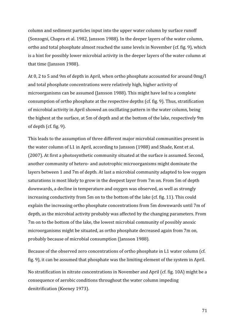
Total phosphate concentrations of L1 decreased with depth in November (cf. fig. 9),
which could be a result of higher microbial activity in the upper layers of the water
71
column and sediment particles input into the upper water column by surface runoff
(Sonzogni, Chapra et al. 1982, Jansson 1988). In the deeper layers of the water column,
ortho and total phosphate almost reached the same levels in November (cf. fig. 9), which
is a hint for possibly lower microbial activity in the deeper layers of the water column at
that time (Jansson 1988).
At 0, 2 to 5 and 9m of depth in April, when ortho phosphate accounted for around 0mg/l
and total phosphate concentrations were relatively high, higher activity of
microorganisms can be assumed (Jansson 1988). This might have led to a complete
consumption of ortho phosphate at the respective depths (cf. fig. 9). Thus, stratification
of microbial activity in April showed an oscillating pattern in the water column, being
the highest at the surface, at 5m of depth and at the bottom of the lake, respectively 9m
of depth (cf. fig. 9).
This leads to the assumption of three different major microbial communities present in
the water column of L1 in April, according to Jansson (1988) and Shade, Kent et al.
(2007). At first a photosynthetic community situated at the surface is assumed. Second,
another community of hetero- and autotrophic microorganisms might dominate the
layers between 1 and 7m of depth. At last a microbial community adapted to low oxygen
saturations is most likely to grow in the deepest layer from 7m on. From 5m of depth
downwards, a decline in temperature and oxygen was observed, as well as strongly
increasing conductivity from 5m on to the bottom of the lake (cf. fig. 11). This could
explain the increasing ortho phosphate concentrations from 5m downwards until 7m of
depth, as the microbial activity probably was affected by the changing parameters. From
7m on to the bottom of the lake, the lowest microbial community of possibly anoxic
microorganisms might be situated, as ortho phosphate decreased again from 7m on,
probably because of microbial consumption (Jansson 1988).
Because of the observed zero concentrations of ortho phosphate in L1 water column (cf.
fig. 9), it can be assumed that phosphate was the limiting element of the system in April.
No stratification in nitrate concentrations in November and April (cf. fig. 10A) might be a
consequence of aerobic conditions throughout the water column impeding
denitrification (Keeney 1973).
Slight decrease in ammonium concentrations connected to slightly increasing nitrate
concentrations at the bottom of L1 in April (cf. fig. 10B) leads to the assumption of
microbial nitrification (Keeney 1973). April and November ammonium concentrations
were very similar, in contrast to other ion concentrations. This might be a consequence
of constant ammonium inputs by surface runoff, rain and groundwater.
Nitrogen concentrations of L1 did not seem to limit microbial activity, as no zero
concentrations in ammonium and nitrate were observed (cf. fig. 10), even that
concentrations were low. Thus, constant nitrogen inputs into L1 could be a possible
cause, which might lead to nitrogen accumulation over time.
In April, L4 showed stratification in conductivity, oxygen saturation, pH and
temperature similar to L1 with a slighter increase in conductivity with depth (cf. fig. 11,
12). As L4 is overall shallower than L1, this might be a possible cause for a less defined
stratification in conductivity in April (Boehrer and Schultze 2008).
Lake water quality
L5 ion concentrations were very low (cf. fig. 8), but nitrate and phosphate
concentrations were in range of L1 and L4 (cf. ch. 3.3). L5 was built in 2011 and filled for
the first time in winter 2012/13 with considerable amounts of rain and surface runoff.
The very low ion concentrations reflect the origin of the lake water directly from rain.
Lower ion concentrations and conductivities of L1 in April in comparison to November
(cf. fig. 7 and 8) might be caused by dilution from rain and surface runoff accumulating
in the lakes, as analyses of surface runoff suggests considerable amounts of anion inputs
by rain (cf. fig. 7). As the inflows I1-4 were measured at the beginning of the rainfall
period in November 2012, it can be assumed that they transported salts and particles
accumulated in the subsoil during the dry season (Chambel and Almeida 1998) to a
greater extent in November as at the end of the wet season, where most particles and
salts might have been washed out already. Thus, ion concentration input into the lakes
by inflowing surface runoff might have been much lower at the end of the wet season
(Hill and Neal 1997), which could explain the relatively low ion concentrations of the
lakes in April 2012 in relation to the ion concentrations of I1-4 in November.
73
Furthermore, the positions of L1 November and April samples in the Piper diagram
indicate slight dilution of L1, as partitions of ion slightly changed between the seasons,
but ion concentrations did change substantially (cf. fig. 5,7,8). Input by surface runoff
into L1 might have changed ion composition, which could explain the slight change of L1
position in the Piper diagram between the seasons.
Especially potassium input seemed to be relatively high, as potassium concentrations, in
contrast to all other measured ions of L1, were even higher than in November, (cf. ch.
3.3).
Overall low ion concentrations of L4 in November (cf. fig. 7) might indicate low
influences of groundwater on the lake during the dry season. But it has to be considered,
that only the surface of the lake was analyzed and thus no assumptions can be made for
the deeper layers of L4 in November. In April, L4 had overall higher or similar ion
concentrations in comparison to November. Especially L4 sodium, chloride and
alkalinity concentrations were much elevated in April (cf. ch. 3.3). The change of
position in the Piper diagram of L4 between the seasons indicates a change in water
composition (cf. fig. 5). This might have been caused by ion inputs from surface runoff,
rain and groundwater inflow during the wet season. L4 is shallower and smaller than L1
(cf. table 1 and fig. 3) and thus has a smaller volume, which means that the ion inputs
during the wet season could probably raise lake water ion concentrations to a greater
extent and much more quickly than in L1.
L4 phosphate and nitrate concentrations did not follow this pattern, as November values
were higher than April values (cf. ch. 3.3). This could be a result of phosphate fixation in
the sediment during winter (Boström, Andersen et al. 1988, Gächter and Müller 2003) as
well as of dilution by rain and inflows. In comparison with L1, April L4 nitrate
concentrations were still higher (cf. ch.3.3).
The relatively high nutrient concentrations of L4 in comparison to L1 (cf. ch. 3.3.1 and
3.3.5) might be a result of the location of L4. It is situated below agricultural terraces,
from where leaching of nutrients is bound to occur (cf. table 1) (Paralta, Carreira et al.
2007).
Very low oxygen saturation levels in April at the bottom of L1 and L4 indicate possible
anoxia in the sediment (cf. fig. 11A and 12A). Upwelling of low oxygen waters from the
deeper layers at the beginning of the mixing period in autumn can cause generally low
oxygen concentrations throughout the water column and affect biological communities
(Morais, Serafim et al. 2007).
Anoxia in the sediment of L1 and L4 during summer could cause phosphate release from
the sediment and might affect the benthic fauna (Boers and van Hese 1988, Boström,
Andersen et al. 1988, Karlson, Rosenberg et al. 2002). Hence, phosphate released by the
sediment in summer probably mixes into the water column during the mixing period in
autumn. This could promote primary production and growth of cyanobacteria (Morais,
Serafim et al. 2007) The observed high November ortho and total phosphate
concentrations of L1 and L4 underline these assumptions (cf. fig. 9 and chapter 3.3.).
Furthermore, particulate phosphate input from surface runoff might have substantially
contributed to the overall high total phosphate concentrations of the lakes. This
assumption is strengthened by the observation that the lakes water was very turbid in
November. Particulate phosphate from runoff might exhibit low bioavailability
(Sonzogni, Chapra et al. 1982) and thus might not be able to contribute to microbial
growth in a great extent.
As the sediment layer of L1, L4 and L5 is relatively young and thus probably still thin,
processes of phosphate immobilization and release by the sediment might develop over
time with more intensity. This could increase the risk of cyanobacteria bloom in
summer, when high light and eventually low nitrate availabilities foster cyanobacterial
growth (Morais, Serafim et al. 2007). Cyanobacteria can produce metabolites, such as
microcystins, which were reported to be toxic to wildlife and livestocks and might cause
human fatalities (Mez, Beattie et al. 1997, Jochimsen, Carmichael et al. 1998).
Additionally, phosphate can be expected to further accumulate in the lakes, due to the
measured high ortho phosphate concentrations of rainfall and phosphate input by
temporary inflows (cf. fig. 7). As reported by Price (1999), nutrient leaching from
agricultural areas and municipal sources increase the risk of toxic algae bloom that
could affect the water supply. Therefore the prevention of anthropogenic and
agricultural phosphate inputs into the lakes is crucial for future lake ecology and
sustainability of the research area.
75
Relatively high ion concentrations of L1 and high conductivities of L2 and L3 in
November (cf. fig. 6 and 7) could cause increases in soil and groundwater salinity when
used for irrigation (Stigter, Carvalho Dill et al. 2006, Sequeira 2010).
Overall, seasonal variations of the water quality observed in the research area covered a
wide range, as a result of climate seasonality and particularly rainfall and solar heating
(Chapman 1996). Because of this, establishment of seasonal monitoring programmes for
estimations of water quality is essential (Simeonov, Stratis et al. 2003, Serafim, Morais et
al. 2006). Additionally, monitoring of soil salinity should be applied.
Differences between lakes
Slight to moderate variations in temperature, pH and oxygen saturation between the
analyzed lakes of the research area (cf. ch. 3.3) indicate varying ecological situations of
the single lakes, reflecting the different geographical locations and lake morphologies as
well as environments of the lakes, some of them influenced by agriculture. Overall
similarities in conductivity and stratification indicate rather small differences in lake
ecology and stratification between the lakes. But differences in nutrient concentrations,
probably caused by varying agricultural influences on the single lakes, should be
considered for further monitoring.
4.1.6 Rain water
Chlorite, sulfate, phosphate and nitrate inputs by rain seem to contribute substantially
to the respective ion concentrations of surface- and groundwaters in the research area
(cf. fig. 7 and ch. 3.4). Particularly chloride input by rain has to be considered for further
monitoring studies, if chloride mass balances would be applied (Gee, Zhang et al. 2005) .
The research site is located at 30km distance to the coast of the Atlantic and thus can be
assumed to be influenced by chloridic rains coming from the sea. Ion concentrations of
rain seem to oscillate, as rain ion concentrations differed between the samples (cf. fig. 7).
Chlorite, sulfate, phosphate and nitrate concentrations in surface waters of the area
seem to be influenced not by rain ion inputs alone, as surface water ion concentrations
were overall higher than rain ion concentrations (cf. fig. 7 and 8). Other possible ion
inputs into surface waters might originate from surface runoff and/or groundwater.
Sample R1 showed abnormally high ion concentrations, especially ammonium, which
could be a result of oscillations in the atmosphere ion concentrations or contamination
during sampling or analysis (cf. fig. 7).
4.1.7 Ion Balances
Some samples had ion balances exceeding ±5%. The maximum deviance was 12% at I4
in November and -9% at SW10 in April. These could be caused by sampling and
transport or might be a result of cations bond in chemical complexes that could not be
broken up during analysis (Hölting and Coldewey 2013). Most ion balances were in the
appropriate range of ±5%, thus the obtained results provide overall reliable
informations about water quality in the research area.
4.1.8 Isotopic composition of ground- and surface waters
δ 18O and δ ²H results indicate a trend of heavier waters in the northern and lower area
of the research area (cf. fig. 14). In detail, S1, W2 and L1 that are situated at the northern
end of the valley (cf. fig. 3) showed a relatively heavy isotopic signature, while SW5, 7
and 8 and L4, located in the southern and steeper part of the valley, exhibited relatively
light isotopic signatures more similar to rain water (cf. fig. 3 and 14).
Thus, the influence of evaporation on the waters during their way down through the
valley is reflected on the isotopic data, as evaporation causes enrichment in both heavy
isotopes, δ 18O and δ ²H (Gibson, Edwards et al. 1993). According to the authors,
meteoric waters that have undergone evaporation display systematic enrichment in
both δ 18O and δ ²H, resulting in a divergence from the meteoric water line along
evaporation lines with slopes of less than 8 and often in the range 4 to 6. The obtained
evaporation line matches these findings.
77
Another factor contributing to changes in isotopic water composition could be microbial
activity as microorganisms contribute to isotope fractionation by assimilating the lighter
isotopes (Knöller, Vogt et al. 2006).
Rain sample R3 showed an influence of evaporation, as its location was closer to the
local evaporation line than to the meteoric water line (cf. fig. 14). This might be a result
of the sampling procedure in an open beaker for several hours.
The calculated mean annual isotopic signature of rain almost matches the isotopic
composition of R3 (cf. ch. 3.5.1). But isotopic compositions of rain in the research area
might vary throughout the seasons, because of temperature-dependent effects during
condensation of atmospheric vapor and air-mass history. As consequence, variations in
the isotopic composition of precipitation result in seasonal shifts along the meteoric
water line (Dansgaard 1964).
Isotopic signature of L1 indicates the origin from rain combined with influences of
evaporation as δ 18O and δ ²H values are much heavier than rain values and located near
to the evaporation line (cf. fig. 14).
In April, a clear overall difference between ground- and surface water isotopic
signatures was observed, most probably due to greater influence by evaporation (cf. fig.
14). In contrast, isotopic signatures in November indicate great variation in evaporation
influences on waters of the research area. The influence of evaporation was greater in
November than in April (cf. fig. 14). Less variation of April isotopic signatures can be
assumed to be caused by dilution of the waters with rain during the wet season. This
reflects seasonal climatic variations of dry and hot summers and wet winters as well as
the different hydrogeological situations of the single wells and water bodies. Therefore it
has to be taken into account that quality of waters in the research area is influenced by
varying parameters.
Isotopic stratification of L1 matches the results obtained from ion concentrations and
the hypothesis of disposition of old lake water in the deeper layers in April (cf. fig. 15).
In November, isotopic signatures showed no stratification of the water column,
matching the results of ion concentrations and other parameters (cf. fig. 15).
Isotopic signatures of November indicate elevated influence of evaporation on L1 water
compared to April, due to enrichment of heavy isotopes in November. This matches the
climatic seasonality of the region.
4.2. Interactions between ground- and surface water
4.2.1 Groundwater leakage into lakes
Groundwater leakage into L1 can be assumed to occur mostly in the deeper layers of the
lake, where possible intersections with the groundwater table would be located. But
isotopic signatures of L1 indicate no substantial influence of groundwater in the deeper
layers. Groundwater leakage into L1 would be reflected on the isotopic results measured
in L1, but L1 November isotopic results were much lower than groundwater isotopic
results (cf. fig. 14 and 15). Therefore little influence of groundwater leakage on L1 in
November can be assumed. A possible groundwater inflow into L1 in April seems to be
relatively small, as April isotopic compositions of L1 were clearly enriched by heavy
isotopes compared to groundwater, especially in the lower layers of the lake (cf. fig. 14
and 15).
In order to determine annual volumes of eventually inflowing groundwater into L1, lake
water and groundwater samples from the area around L1 should be analyzed
throughout the year. This would enable to apply stable isotope mass balance with mean
annual δ 18O and δ ²H values from rain, lake and groundwater (Krabbenhoft, Bowser et
al. 1990).
In November, conductivity of L1 and L2 was similar to conductivity of shallow wells,
whereas conductivities in April of all measured lakes showed lower values than
conductivities of all wells (cf. fig. 6). Similar conductivities of shallow wells, L1 and L2
might indicate a rather high influence of groundwater on the lakes during the dry
season. But isotopic signatures revealed no similarities between L1 and the shallow or
deep wells in November, which contradicts the assumption of inflowing groundwater in
November. The relatively high lake water conductivities in November can be assumed to
be a result of evaporation. As isotopic composition of L2 was not measured in
November, groundwater inflow into L2 in November is not known.
79
L4 showed ion concentrations very similar to rain water in November; hence mainly
rainwater might have been in the lake.
The relatively low lake water conductivities of all measured lakes in April (L1, L2, L3, L4,
L5) could be a hint for a low influence of groundwater on lake water compositions
during the wet season (cf. fig. 6). This matches the position of the surface waters in April
above the groundwaters on the evaporation line (cf. fig. 14), indicating no similarities
between ground- and surface waters, except for SW1.
Conductivity of L5 in April was very low and ion concentrations were similar to rain
water (cf.fig. 6, 7 and 8) which underlines the assumption of no remarkable amounts of
groundwater in the lake at that time.
Water tables of SW3 could give a rough idea of interactions between SW3 and L5. In
comparison to October 2012, SW3 had a much higher water table in October 2013 (cf.
fig. 4). As discussed in chapter 4.1.1, SW3 water table seems to be highly influenced by
L5. The difference of SW3 water tables in October 2012 and October 2013 was about
4m, which is much more than the difference between October 2012 and 2013 of other
shallow wells showing differences of around 2.5m (cf. fig. 4). This could be a result of the
construction of L5. But to know the volume of exfiltrating water, data of the leakage
coefficients of the lake sediments and lake floors are needed to apply Darcy´s law
(Hölting and Coldewey 2013). These values could not be measured and should be
analyzed for further research.
To compare yearly mean water tables of SW3 over longer time periods with varying
annual precipitations, more research has to be done. Then a possible influence of L5 on
the surrounding groundwater tables might be confirmed or rejected.
Hence, SW3 could be useful for monitoring groundwater tables in the water retention
space of L5 during summer when water of L5 is not flooding SW3, but probably
influences the groundwater tables of the area. If L5 water tables would be monitored as
well, it would be possible to detect exfiltration into the groundwater in the area around
SW3 by comparing water tables of SW3 and L5 (Hölting and Coldewey 2013).
4.2.2 Lake 4 leakage into SW1
Isotope analysis results of SW1 and L4 show no clear influence of L4 on SW1 in
November, but standard deviations of April δ 18O values of SW1 and L4 were
overlapping (cf. table 5). This might indicate SW1 to be influenced by L4 in April.
Standard deviations of SW1 and L4 δ ²H values did not overlap in April, but values were
close to each other (cf. table 5). Additionally, SW1 isotopic values measured in April
were located between surface and groundwater isotopic compositions (cf. fig. 14).
Furthermore, SW1 April conductivity and ion concentrations were very low in
comparison to other shallow wells and similar to L4 (cf. fig. 6, 7 and 8).
Thus, it can be assumed that April SW1 water was leaking water from L4 probably
mixed with some groundwater. Especially measured chloride concentrations go in line
with this assumption, as April SW1 chloride concentrations were very low in
comparison to the other wells and similar to L4 concentrations (cf. fig. 8).
In November, SW1 seemed to be influenced mainly by groundwater, as ion
concentrations, conductivity and isotopy were in the range of most other shallow wells
(cf. fig. 6, 7, 8, 14 and table 5). However, an influence of L4 on SW1 cannot be excluded
for November.
As SW1 seemed to be fed mainly by groundwater in November 2012, possible effects on
the local groundwater table by pumping during the dry season might occur. This could
eventually lead to consequences for the surrounding vegetation and has to be
considered for further monitoring. But as L5 can be expected to fill up over time and to
influence the quantity of groundwater in the valley, the groundwater situation in SW1
area might change during the next years.
Furthermore, sodium and chloride concentrations of SW1 and SW4 increased much less
between the seasons compared to concentrations of other shallow wells (cf. fig. 7 and 8).
As SW1 and SW4 are located in the valley below L5 and L4, both wells can be assumed to
be influenced by leaking lake water, showing relatively low sodium and chloride
concentrations in April (cf. fig. 8 and ch. 4.1).
81
Therefore, water quality of the water supply in the village seems to be highly dependent
on L4 and probably also L5 water quality. The influence of L5 on SW1 might increase
over time.
4.2.3 L1 leakage into S3
Similar ion concentrations in November of S3 and L1 indicate a possible leakage of L1
into S3. However, a strong influence by groundwater on S3 cannot be excluded, as S3 ion
concentrations were in the range of groundwater ion concentrations of November (cf.
fig. 7). S3 showed the highest enrichment of heavy isotopes compared to all other waters
of the research area. Thus, S3 can be assumed to have been highly influenced by
evaporation, as S3 water accumulated below the L1 dam in a shallow basin exposed to
the sun. Isotopic results did not show similarities between S3 and L1 in November and
between S3 and groundwater (cf. fig. 14). Therefore it can be assumed that only small
amounts of water came out of the spring at that time.
In April, S3 was flooded by L1 outflow through pipes in the middle of L1 dam, thus April
conductivity and ion concentrations of S3 were almost identical with L1 (cf. fig. 6 and 8).
4.3 Water supply
SW1 provides drinking water for the village, which in terms of ion concentrations has
good quality (cf. ch. 3.2). If current agricultural practices in the watershed of SW1 do not
change the water can be expected to stay safe with regards to these parameters. The
implementation of SW1 marks a step towards sustainable water supply compared to the
former practice of deep well pumping. This is especially true as the well seems to be fed
by the overlying lake L4 (cf. ch. 4.2.2) which was still filled with water in November
2012, after almost two years of very poor rainfall (Weather Station Beja 2011, Weather
Station Beja 2012). In fact, nowadays the water supply of the village not only relies on
groundwater but to a great extent on the water retention space of L4 and probably the
overlying retention spaces of L5 and other smaller lakes. This can be assumed to
contribute to the groundwater flow in the valley, where SW1 is located (cf. ch. 4.2.2 and
4.1.1). But it has to be considered, that with future accumulation of sediments in L4 and
L5, leakage of the lakes might reduce, because of decreased permeability of sediment
layers at the lake bottoms (Hölting and Coldewey 2013).
L4 was assumed to be influenced by nutrient leaching from the surrounding agricultural
terraces (cf. ch. 4.1.5). Therefore regular control of SW1 water quality is crucial.
Another important issue connected to lake water nutrient contents is the possible
growth of cyanobacteria (Morais, Serafim et al. 2007), which could affect human and
animals health (cf. ch. 4.1.5). The growth of blue-green algae during the dry season has
been reported e.g. for the water reservoir Alqueva Dam in South Portugal, which was
classified as eutrophic system (Morais, Serafim et al. 2007). Since substantial
cyanobacteria growth is connected to high water temperatures and high phosphate
concentrations (Morais, Serafim et al. 2007), critical formation of blue-green algae in
lakes on the research site might occur in summer, when water concentrations of
phosphate rise substantially. However, blooms in winter have been reported for South
Portuguese waters as well (Galvao, Reis et al. 2008). This could happen, when
agricultural and land management practices would change, e.g. by introduction of
livestock, waste water disposal into the lakes or higher application of fertilizers in the
catchment area.
Without fail, regular seasonal monitoring of the water qualities on the research site is
crucial for safe water supply and environmental conservation.
Ion concentrations of the analyzed tap water samples did not exceed threshold limits (cf.
ch. 3.2.), except for iron concentrations of the storage tanks. Measured ferrous iron
concentrations in the water supply chain leads to the assumption of substantial amounts
of iron accumulating in the pipe system connected directly to SW1. As ferrous iron
concentrations in the water in the storage tanks was much lower compared to the water
of SW1 (cf. ch. 3.2.), absent iron can be assumed to remain in the pipes as a corrosive
layer on the pipe walls (Lin, Ellaway et al. 2001) or to accumulate in parts at the bottom
of the storage tanks as iron(III).
To prevent possible further corrosion of the pipes and to lower ferrous iron
concentration in the water supply, measures that aerate the water directly after leaving
the well should be applied. Aeration followed by rapid sand filtration is usually
83
recommended for oxidizing ferrous iron in waters with high iron concentration, which is
cheaper than application of chemicals so that costs for chemicals can be avoided (Wong
1984).
4.4. Waste water management
The effectiveness of the septic tank seems to be quite good, as WW2 nutrient
concentration was around ten times lower than WW3 concentrations in April (cf. fig.
16). But as WW1 reed bed phosphorus outputs were exceeding EU limits in both months
and differences in nutrient concentrations between WW1 and WW2 were relatively
small (cf. fig. 16 and ch. 3.6), the capacity of the reed bed seems not to be appropriate.
Therefore the size of the reed bed should be adjusted or waste water treatment should
be improved elsewise.
4.5 Monitoring
4.5.1 Water quality and lake ecology
As mentioned above, further monitoring of water quality of the research area in relation
to water supply is crucial for safe water supply. Because of high seasonal and
interannual climatologic variations, monitoring that provides representative and
reliable informations about water qualities is crucial (Simeonov, Stratis et al. 2003,
Serafim, Morais et al. 2006).
Especially possible nutrient input by agriculture and eventual municipal discharge as
well as cyanobacteria density should be measured regularly (cf. ch.4.1.5 and 4.3).
Monitoring of lake stratifications would help to understand lake ecology and to track
possible changes in lake ecology over time, especially with regard to eutrophication (cf.
ch. 4.1.5). This could be of special interest in case of further aquaculture application.
The observed variations in lake ecology between the different lakes of the research site
might lead to differing effects of possibly changing environmental parameters, such as
mean annual temperature, wind velocity, nutrient input and surface runoff. This should
be considered for further monitoring.
Additionally, monitoring of waste water nutrient loads is essential for environmental
conservation (cf. ch.4.4).
4.5.2 Groundwater recharge
To monitor sustainability of the water supply at Tamera ecovillage quantitatively,
recharge rates together with extraction rates should be evaluated regularly. Higher
extraction rates than recharge rates over long time periods would lead to
overexploitation.
Various direct and indirect methods for monitoring groundwater recharge on the
research site could be applied as listed in Paralta and Oliveira (2005) and Scanlon, Healy
et al. (2002). Among them are:
-Measurement of piezomteric fluctuations
Monitoring of water tables and precipitation over long time periods with fixed data
loggers and measurements of the hydraulic conductivity could be applied for measuring
the relationship between groundwater table and recharge rates and thus enable
assessment of long term effects of the water retention landscape on groundwater tables.
Thereby comparison between groundwater tables of the study site and of neighboring
valleys would enable to evaluate effects of the water retention landscape on
groundwater dynamics on the study site in comparison to aquifers of non-influenced
valleys.
85
-Water and physical balance studies
By implementation of a local weather station and analysis of weather data, exact
precipitation and evapotranspiration values could be obtained for physical balance
studies.
Additionally, monitoring of precipitation and water volumes of the area accompanied by
constant measurements of outflowing water masses from the research area would
enable water balance studies.
4.5.3 Tracer techniques
Application of long term chloride mass balance studies could help to understand
groundwater recharge processes of the research area in more detail. Required data
include annual precipitation, total chloride input from dry fallout and precipitation, as
well as pore water chloride concentrations (Gee, Zhang et al. 2005).
Long term evaluation of lake, groundwater and rain δ 18O and δ ²H values would enable
further studies about ground-and lake water interactions by applying the stable isotope
mass balance method (Krabbenhoft, Bowser et al. 1990).
Conclusions
Overall great seasonal variations of ground- and surface water quality in the water
retention landscape were observed. Consequently seasonal measurements of water
quality and groundwater recharge are crucial for further monitoring. Influences of
agriculture and evaporation might affect water quality of artificial lakes and aquifer of
the water retention landscape over time. But if current agricultural practice is continued
and regular monitoring of water quality is applied, water supply seems to be safe in
terms of the measured biogeochemical parameters.
The measured high nutrient outputs from the waste water system of the village into the
surrounding surface waters lead to the conclusion that a change in waste water
management of the village is needed. The reed bed should be adjusted to the discharge
rates of the settlement and monitoring of nutrient outflows into surface waters from the
reed bed should be applied regularly in order to prevent further eutrophication of the
lakes.
L4 and L1 seemed to leak into the aquifer system at the beginning of the wet season and
leakage of L5 during the wet season was assumed. No substantial groundwater inflow
into the lakes was found. However, it is not sure whether lakes of the water retention
landscape exfiltrate into the aquifer constantly.
Finally it can be concluded that the water supply at Tamera ecovillage by the artificial
lakes of the water retention landscape secures sustainable water supply from surface
runoff and rain, thus being much more sustainable than the former deep well pumping
in the area. This could be a model for agricultural and land regeneration of semi-arid
regions.
87
Acknowledgements
I want to thank Dr. Christine Laskov and Prof. Dr. Heinz-R. Köhler for supervising this
work and thus enabling this study. Especially good advices from Christine Laskov
supported this study substantially.
I am very grateful to Monika Hertel for her support during the lab analysis and for
always lending a helping hand. I also want to thank Bernd Steinhilber for supporting me
in the isotope analysis.
Furthermore my thanks go to Christoph Ulbig from the ecology team of Tamera who
provided me with data and was always open to my questions. Additionally, I am greatful
to the inhabitants of Tamera ecovillage for providing me with everything I needed
during the sampling.
My thanks go to Hans-Martin Krause for proofreading the text with great dedication and
for lending a helping hand during the sampling.
Special thanks go to Jürgen Daum, Susanne Hartleb, Sylvia Paglialonga, Peter and Rosa
Hartleb, Dave Tijok, Anke Brüchert, Hans-Martin Freudenreich, Helene Elsässer, Petra
Schumacher and Julian Wider for supporting this study financially.
I am very grateful for all the support I received from friends and family during the work
on this study.
References
Boehrer, B. and M. Schultze (2008). "Stratification of lakes." Reviews of Geophysics 46(2): RG2005.
Boers, P. C. M. and O. van Hese (1988). "Phosphorus release from the peaty sediments of the Loosdrecht Lakes (The Netherlands)." Water Research 22(3): 355-363.
Boström, B., et al. (1988). Exchange of Phosphorus Across the Sediment-Water Interface. Phosphorus in Freshwater Ecosystems. G. Persson and M. Jansson, Springer Netherlands. 48: 229-244.
Carreira, P. M. M., et al. (2005). Isotopic composition of rain and water vapour samples from Lisbon region: a characterization of monthly and daily events. Isotopic composition of precipitation in the Mediterranean Basin in relation to air circulation patterns and climate. Vienna, Austria, Isotope Hydrology Section, International Atomic Energy Agency.
Chambel, A. (2006). Groundwater in semi-arid mediterranean areas. Groundwater and Ecosystems-NATO science series: Earth and environmental sciences. A. Baba, F. W. F. Howard and O. Gunduz, Springer.
Chambel, A. and C. Almeida (1998). Origin of highly mineralised waters in a semi-aridarea of the South Portugueses Zone (Portugal). XXVIII Congress of the International Association of Hydrogeologists and the annual meeting of the American Institute of Hydrologists. B. e. al. Las Vegas, Nevada, USA.
Chapman, D. (1996). Water Quality Assessments - A Guide to Use of Biota, Sediments and Water in Environmental Monitoring-Second Edition Cambridge , GB, Chapman & Hall.
Correia, T. P. (1993). "Threatened landscape in Alentejo, Portugal: the ‘montado’ and other ‘agro-silvo-pastoral’ systems." Landscape and Urban Planning 24(1–4): 43-48.
Cunha, L. V., et al. (2006). Alterações Climáticas em Portugal: Cenários, Impactos e Medidas de Adaptação, projecto SIAM II. Lisbon, Portugal.
Dansgaard, W. (1964). "Stable isotopes in precipitation." Tellus 16(4): 436-468.
deVries, J. J., et al. (2000). "Groundwater recharge in the Kalahari, with reference to paleo-hydrologic conditions." Journal of Hydrology 238: 110–123.
Dokulil, M., et al. (2001). Ökologie und Schutz von Seen. Stuttgart, UTB.
Domingues, R. B., et al. (2007). "Impact of reservoir filling on phytoplankton succession and cyanobacteria blooms in a temperate estuary." Estuarine, Coastal and Shelf Science 74(1–2): 31-43.
EEA (2010). Freshwater - National Responses (Portugal) The European environment – state and outlook 2010. Copenhagen, Denmark, European Environment Agency.
Estrela, T., et al. (1996). Water resources problems in southern Europe - An overview report. Copenhagen, Denmark, European Environment Agency.
EU (1991). Directive 91/271/EEC concerning urban waste-water treatment COM/89/0518 E. Council. Brussels, Belgium.
89
EU (1998). Directive on the quality of water intended for human consumption. C. o. Europe, Official Journal of the European Communities 330: 32-54.
Fernandes, P., et al. (2008). Geochemistry of the Baixo Alentejo Flysch Group, South Portuguese Zone: Implications for provenance and palaeoweathering Goldschmidt. Vancouver, Canada.
Furtak, H. and H. R. Langguth (1967). Zur hydrochemischen Kennzeichnung von Grundwässern und Grundwassertypen mittels Kennzahlen. IAH-Congress. Hannover, Germany. 7: 86-96.
Gächter, R. and B. Müller (2003). Why the phosphorus retention of lakes does not necessarily depend on the oxygen supply to their sediment surface. Limnology and Oceanography. Waco, TX, ETATS-UNIS, American Society of Limnology and Oceanography. 48: 929-933.
Galvao, H. M., et al. (2008). "Cyanobacterial blooms in natural waters in southern Portugal: a water management perspective." Aquatic Microbial Ecology 53(1): 29-140.
Gee, G. W., et al. (2005). "Chloride Mass Balance." Vadose Zone J. 4(1): 72-78.
Gibson, J. J., et al. (1993). "Estimating Evaporation Using Stable Isotopes: Quantitative Results and Sensitivity Analysis forTwo Catchments in Northern Canada." Nordic Hydrology 24: 79-94.
Hill, T. and C. Neal (1997). "Spatial and temporal variation in pH, alkalinity and conductivity in surface runoff and groundwater for the Upper River Severn catchment." Hydrology and Earth System Sciences 1(3): 697-715.
Hölting, B. and W. G. Coldewey, Eds. (2013). Hydrogeologie. Berlin Heidelberg, Springer Verlag.
Holzer, S. (2012). Desert or Paradise: Restoring Endangered Landscapes Using Water Management, including Lake and Pond Construction. East Meon, England, Permanet Publications.
Jansson, M. (1988). Phosphate Uptake and Utilization by Bacteria and Algae. Phosphorus in Freshwater Ecosystems. G. Persson and M. Jansson, Springer Netherlands. 48: 177-189.
Jochimsen, E. M., et al. (1998). "Liver Failure and Death after Exposure to Microcystins at a Hemodialysis Center in Brazil." New England Journal of Medicine 338(13): 873-878.
Karlson, K., et al. (2002). Temporal and spatial large-scale effects of eutrophication and oxygen deficiency on benthic fauna in Scandinavian and Baltic waters: A review. Boca Raton, FL, ETATS-UNIS, CRC Press.
Keeney, D. R. (1973). "The Nitrogen Cycle in Sediment-Water Systems1." J. Environ. Qual. 2(1): 15-29.
Knöller, K., et al. (2006). "Sulfur and Oxygen Isotope Fractionation during Benzene, Toluene, Ethyl Benzene, and Xylene Degradation by Sulfate-Reducing Bacteria." Environmental Science & Technology 40(12): 3879-3885.
Krabbenhoft, D. P., et al. (1990). "Estimating groundwater exchange with lakes: 1. The stable isotope mass balance method." Water Resources Research 26(10): 2445-2453.
Krom, M. D. (1980). "Spectrophotometric determination of ammonia: a study of a modified Berthelot reaction using salicylate and dichloroisocyanurate." Analyst 105(1249): 305-316.
Liebe, J., et al. (2005). "Estimation of small reservoir storage capacities in a semi-arid environment: A case study in the Upper East Region of Ghana." Physics and Chemistry of the Earth, Parts A/B/C 30(6–7): 448-454.
Lin, J., et al. (2001). "Study of corrosion material accumulated on the inner wall of steel water pipe." Corrosion Science 43(11): 2065-2081.
Mez, K., et al. (1997). "Identification of a microcystin in benthic cyanobacteria linked to cattle deaths on alpine pastures in Switzerland." European Journal of Phycology 32(2): 111-117.
Miao, Z., et al. (2012). "Sulfate reduction in groundwater: characterization and applications for remediation." Environmental Geochemistry and Health 34(4): 539-550.
Morais, M. M., et al. (2007). Monitoring the water quality in Alqueva Reservoir, Guadiana River, southern Portugal. Berlin, Germany, Technische Uni Berlin.
Murphy, J. and J. P. Riley (1962). "A modified single solution method for the determination of phosphate in natural waters." Analytica Chimica Acta 27(0): 31-36.
Neal, C. (1988). "Bicarbonate estimation from alkalinity determinations for neutral to acidic low alkalinity natural waters: theoretical considerations " Hydrological Sciences 33(6): 619-624.
Paralta, E., et al. (2007). Assessing agriculture pollution in the Beja aquifer using nitrogen isotopes, South Portugal. International Symposium on Advances in Isotope Hydrology and its Role in Sustainable Water Resources Management. Vienna, Austria, International Atomic Energy Agency.
Paralta, E. and M. Oliveira (2005). Assesing and modelling hard rock aquifer recharge based on complementary methodologies-a cas study in the "Gabbros of Beja" aquifer system (South Portugal). 2nd Workshop of the Iberian Regional Working Group on Hardrock Hydrogeology. Evora, Portugal.
Pereira, M. and D. Figueiredo (2009). "Effects of the Alqueva Dam Reservoir on the Distribution of Steppe Birds." Physical Geography 30(1): 43-63.
Pereira, Z., et al. (2007). "Devonian and Carboniferous palynostratigraphy of the South Portuguese Zone, Portugal –An overview." Comunicações Geológicas 94: 53-79.
Pinho, A. B., et al. (2007). The Baixo Alentejo (Portugal) flysch rocks. The Second Half Century of Rock Mechanics, Three Volume Set, Taylor & Francis.
Price, D. R. H. (1999). "Do reservoirs need ecological management?" Hydrobiologia 395-396(0): 117-121.
Ramos, C. and E. Reis (2002). "Floods in southern Portugal: their physical and human causes, impacts and human response." Mitigation and Adaptation Strategies for Global Change 7(3): 267-284.
Ribeiro, L. and L. V. daCunha (2010). Portuguese groundwater report. Groundwater in the Southern Member States of the European Union: an assessment of current knowledge and future prospects, European Academies Science Advisory Council.
Santos, M., et al. (2008). "Assessing dam implementation impact on threatened carnivores: the case of Alqueva in SE Portugal." Environmental Monitoring and Assessment 142(1-3): 47-64.
Scanlon, B. R., et al. (2002). "Choosing appropriate techniques for quantifying groundwater recharge." Hydrogeology Journal 10(1): 18-39.
91
Scanlon, B. R., et al. (2006). "Global Synthesis of Groundwater Recharge in Semiarid and Arid Regions." Hydrological Processes 20: 3335-3370.
Sequeira, E. (2010). Desertification and salinisation in the Alentejo region, Portugal. Implementing the EU Water Framework Directive: A seminar series on water. Brussels, Belgium, WWF with the support of the European Commission and TAIEX.
Serafim, A., et al. (2006). "Spatial and temporal heterogeneity in the Alqueva reservoir, Guadiana river, Portugal." Limnetica 25(3): 771-786.
Shade, A., et al. (2007). "Interannual dynamics and phenology of bacterial communities in a eutrophic lake." Limnology and Oceanography 52(2): 487-494.
Simeonov, V., et al. (2003). "Assessment of the surface water quality in Northern Greece." Water Research 37(17): 4119-4124.
Smith, S. V., et al. (2002). "Distribution and significance of small, artificial water bodies across the United States landscape." Science of The Total Environment 299(1–3): 21-36.
Sonzogni, W. C., et al. (1982). "Bioavailability of Phosphorus Inputs to Lakes1." J. Environ. Qual. 11(4): 555-563.
Stigter, T. Y., et al. (2006). "Impact of the shift from groundwater to surface water irrigation on aquifer dynamics and hydrochemistry in a semi-arid region in the south of Portugal." Agricultural Water Management 85(1–2): 121-132.
Stookey, L. L. (1970). "Ferrozine---a new spectrophotometric reagent for iron." Analytical Chemistry 42(7): 779-781.
UNESCO (2012). Managing Water under Uncertainty and Risk. The United Nations World Water Development Report 4. Paris, France, United Nations Educational, Scientific and Cultural Organization
Weather Station Beja, P. (2011). "Historical weather 2011." Retrieved 31.12.2013, 2013, from http://weatherspark.com/history/32364/2011/Beja-Portugal.
Weather Station Beja, P. (2012). "Historical weather 2012." Retrieved 31.12.2013 2013, from https://weatherspark.com/history/32364/2012/Beja-Portugal.
Weather Station Beja, P. (2013). "Historical weather 2013." Retrieved 31.12.2013, 2013, from https://weatherspark.com/history/32364/2013/Beja-Portugal.
Wisser, D., et al. (2010). "The significance of local water resources captured in small reservoirs for crop production – A global-scale analysis." Journal of Hydrology 384(3–4): 264-275.
Wong, J. M. (1984). "Chlorination-filtration for iron and manganese removal." Journal of the American Water Works Association 76(1): 76-79.
Wunderly, M. D., et al. (1996). "Sulfide mineral oxidation and subsequent reactive transport of oxidation products in mine tailings impoundments: A numerical model." Water Resources Research 32(10): 3173-3187.