Kinematics of 3D Folding Structures for Nanostructured Origami TM Diplomarbeit submitted by cand.-ing. Tilman Buchner December, 2003 Department of Mechanical Engineering 3D Optical Systems Group Prof. George Barbastathis, PhD RHEINISCH- WESTFÄLISCHE TECHNISCHE HOCHSCHULE AACHEN Werkzeugmaschinenlabor Steuerungstechnik und Automatisierung Prof. Dr.-Ing. Dr.-Ing. E.h. M. Weck Advisor: Dipl.-Ing. Frank Possel-Dölken
Transcript
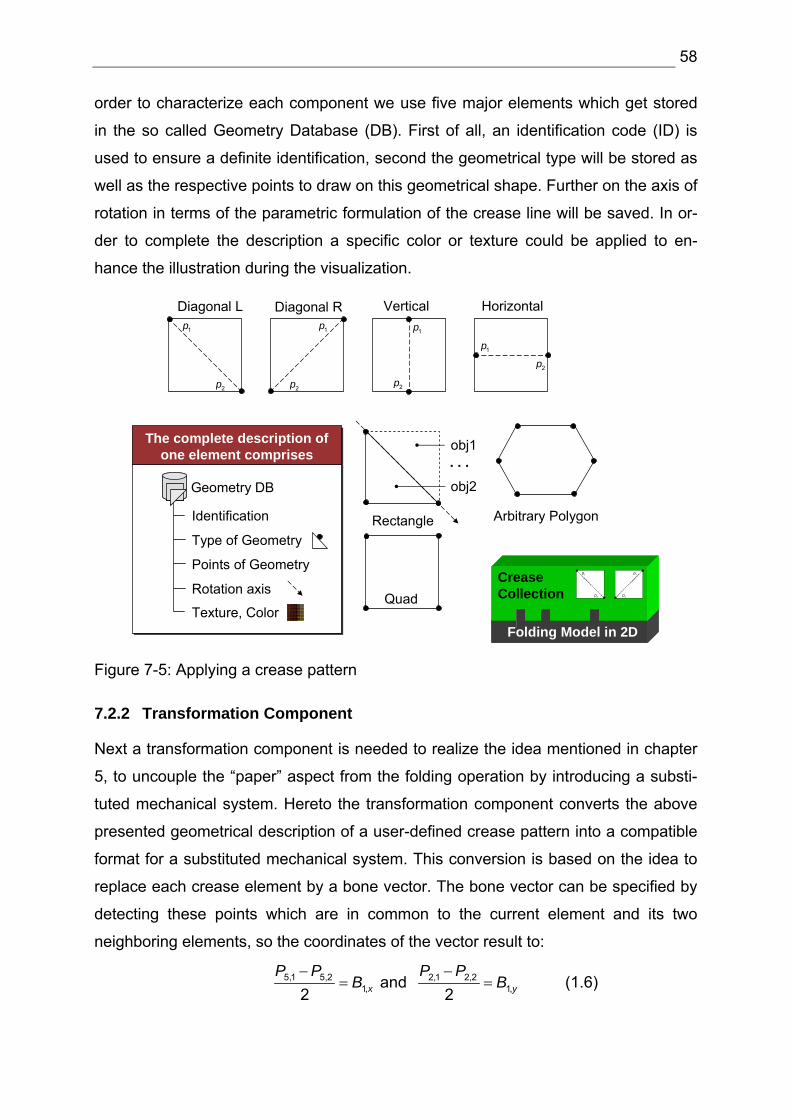
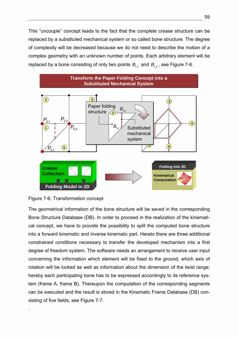
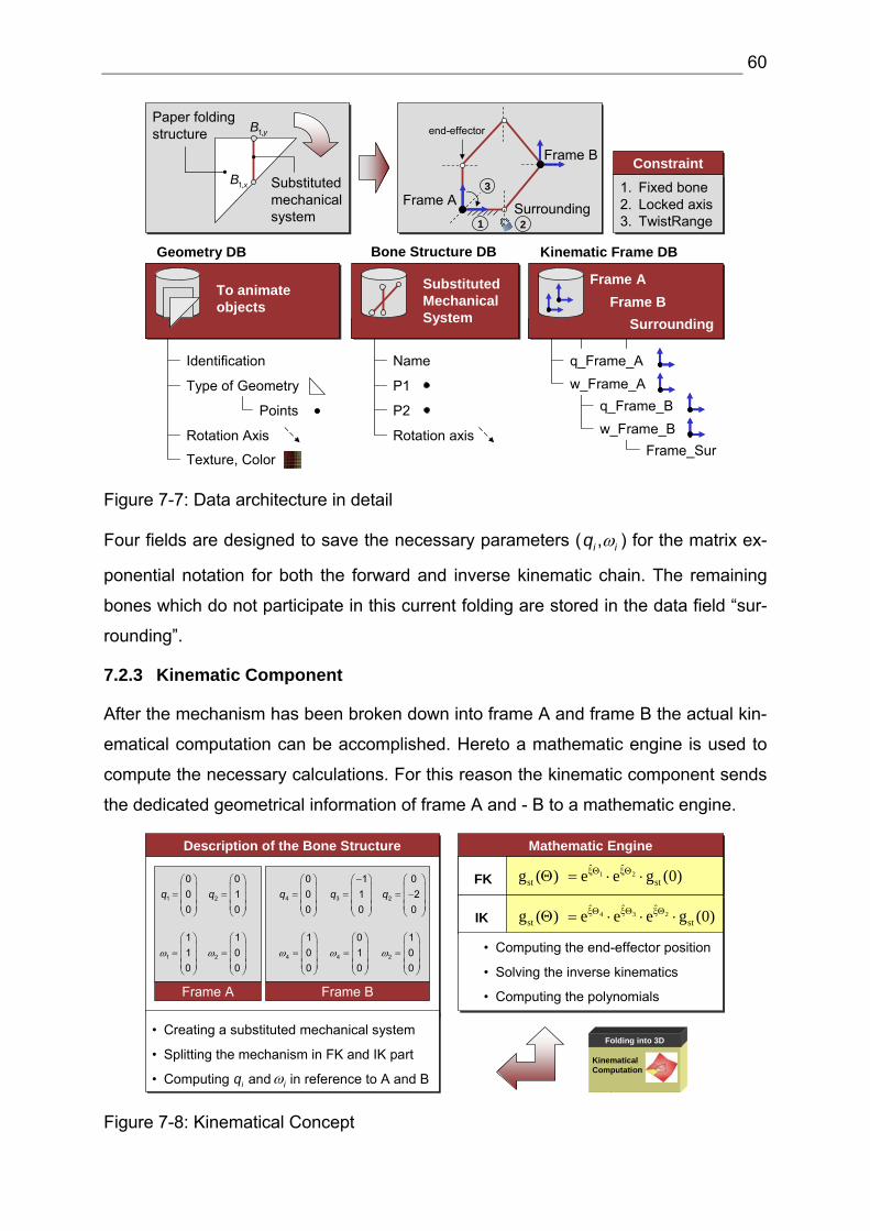
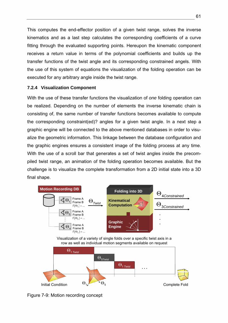
Kinematics of 3D Folding Structures for Nanostructured OrigamiTM
Diplomarbeit
submitted by
cand.-ing. Tilman Buchner
December, 2003
Department of Mechanical Engineering
3D Optical Systems Group
Prof. George Barbastathis, PhD
RHEINISCH-WESTFÄLISCHETECHNISCHEHOCHSCHULEAACHEN
Werkzeugmaschinenlabor
Steuerungstechnik und Automatisierung
Prof. Dr.-Ing. Dr.-Ing. E.h. M. Weck
Advisor: Dipl.-Ing. Frank Possel-Dölken
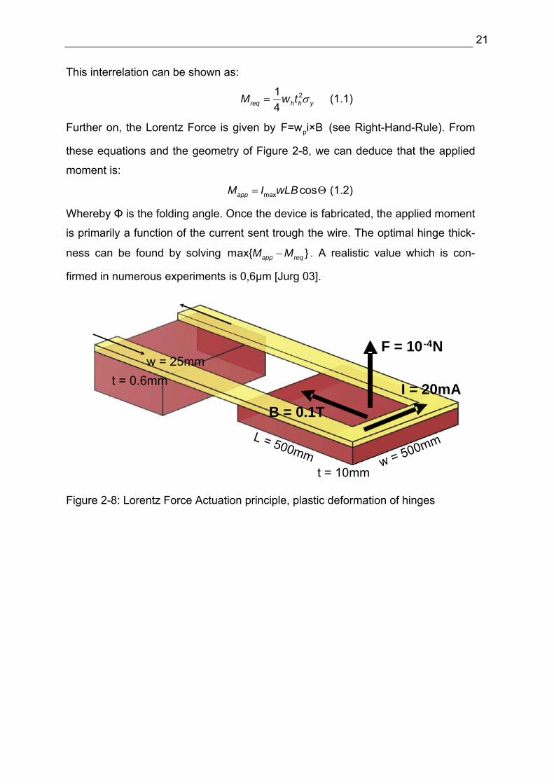
1
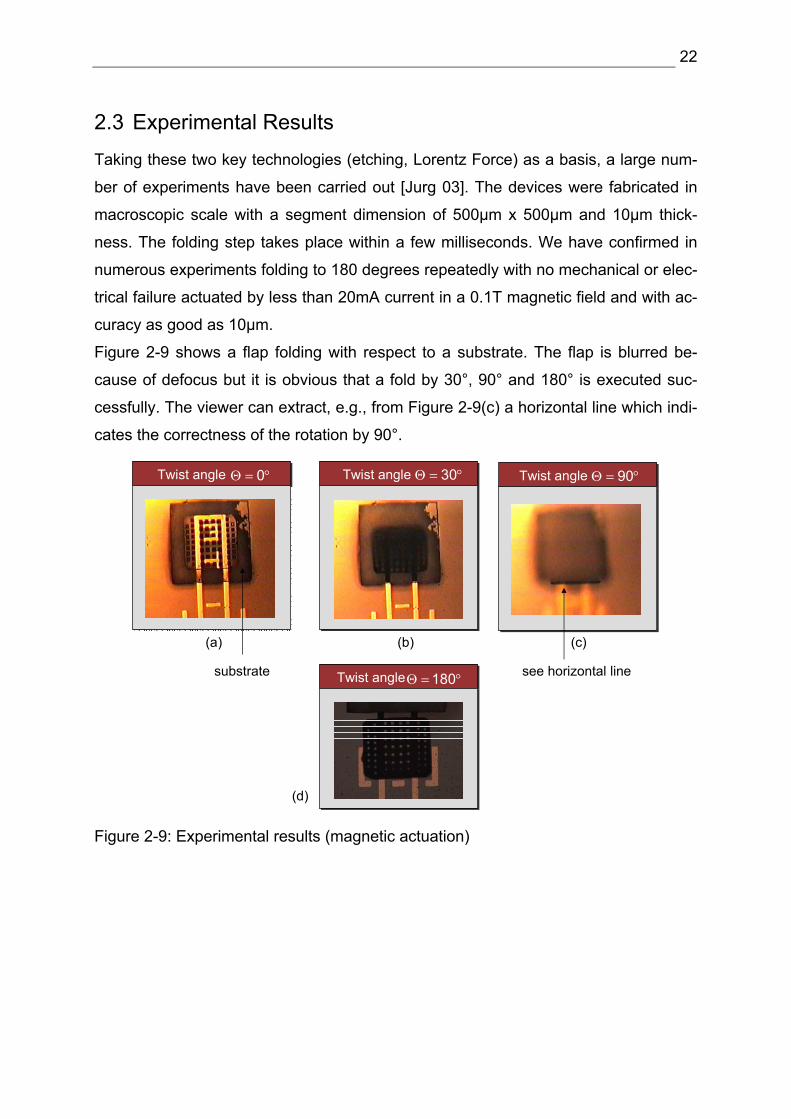
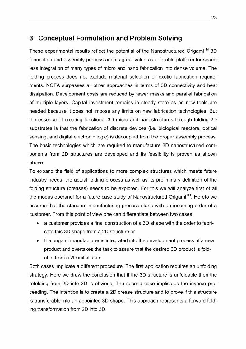
Abstract The 3D Optical Systems Group at MIT investigates Nanostructured OrigamiTM 3D fabrication and assembly. The idea is to assemble complex hybrid (chemical or bio-logical reactors, optical sensing, digital electronic logic, mechanical motion) systems in 3D by using exclusively 2D lithography technology. The 3D shape is obtained by folding the initial 2D membrane in a prescribed way, in a manner reminiscent of the Japanese art of origami (paper-folding). The patterning method (2D nanolithography, nanoimprinting and other techniques) as well as the actuation principle (Lorentz force actuation) which is responsible for initializing the folding process have already been developed and established. The knowledge of the dynamic folding process itself, needed to reach any desired 3D shape from a 2D initial state is to-date unexplored. Hence, the primary objective of this thesis is to determine the motions required to reach the goal (folded state) from a given initial state (unfolded). Hereto general folding operations will be analyzed and a new method to describe its kinematics for any arbitrary structure will be developed. We propose to use origami mathematics in combination with kinematical formulations in the area of robotics and gearing. The most attractive feature of origami is that one can construct a wide variety of complex shapes using a few axioms, simple fixed ini-tial conditions and one mechanical operation, a fold. In a second step, the idea will be pursued to transfer this paper folding concept to a more generally admitted ap-proach which uncouples the paper aspect from the folding operation. Hereby a com-bination of bodies, which are connected by joints, is used to describe the crease structure. As a result, the crease structure is represented in terms of a closed-loop Multi Body System (MBS) with the property that a change of relative motion at one location in-duces a change of relative motion elsewhere. To describe this system, a well-known mathematical method, called screw calculus will be applied. Screw calculus is based on Poinsot’s result that an arbitrary rigid body motion can be described in terms of a translation cascaded with a rotation around the translation axis. The “screw” then is a matrix exponential describing the motion. By cascading several screws together one can describe the motion of articulated rigid body systems, such as robotic manipula-tors and, in our case, origami. The results of the theoretical investigation will be implemented in a design and simu-lation software tool. The application has features to verify and create folding struc-tures as well as to visualize the folding operation on the basis of the above men-tioned kinematics approach.
2
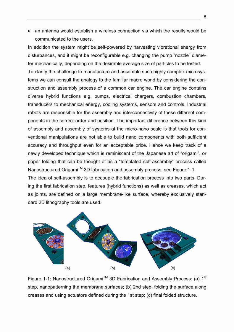
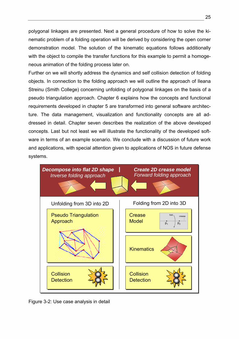
List of Figures Figure 1-1: Nanostructured OrigamiTM 3D Fabrication and Assembly Process. ......... 8
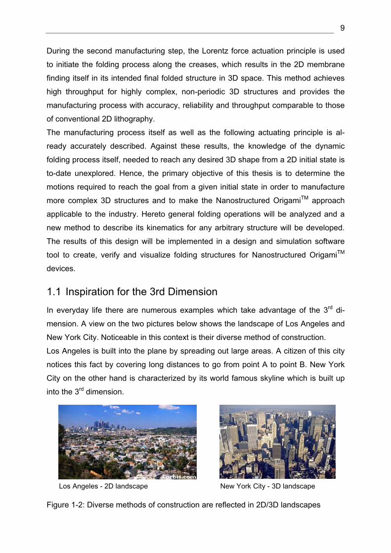
Figure 1-2: Diverse methods of construction are reflected in 2D/3D landscapes ....... 9
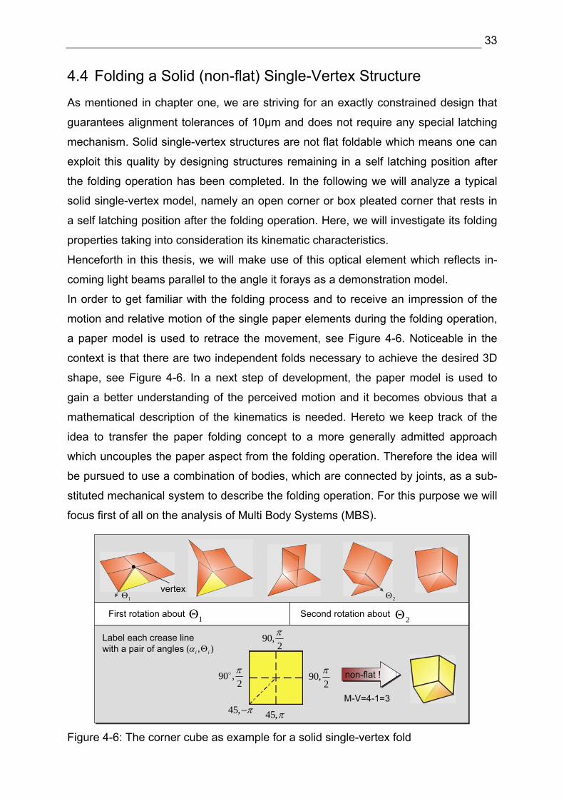
Figure 4-8: Kinematical classification of Multi Body Systems
In order to model this spherical mechanism, joints are necessary to connect two ele-
ments of a MBS with each other. In general, it establishes 6-f holonomic constraints
between these two elements depending on the degree of freedom f. The relative mo-
tion of two bodies connected with a joint could be described with so-called natural or
relative joint co-ordinates β. The natural joint co-ordinates are the angle of rotation
i iβ = Θ and/or displacement i isβ = . Figure 4-9 gives a review of the three basic
joints which can be used to assemble joints with more than 1 DOF by series connect-
ing of these swivel – and shear joints.
36
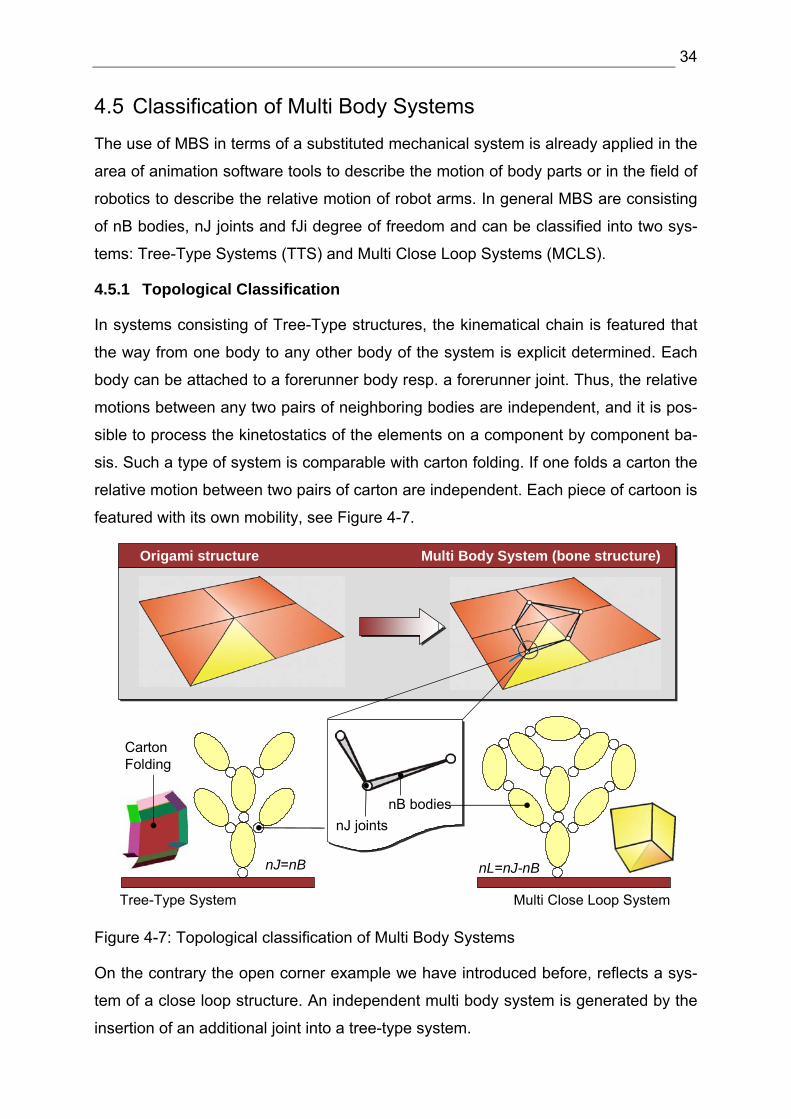
The most general joint is the helical joint (H). Special cases of this joint are the revo-
lute joint (R) (flank lead=0) as well as the prismatic joint (P) (flank lead=1).
In order to create a substituted mechanical system which reflects the kinematical
quality of an open corner we will model the creases as joints, and the uncreased re-
gions as massless rigid bodies, see Figure 4-9. Hereto we will select revolute joints in
combination with massless rigid bodies to simulate the spherical movement.
Helical Joint (H)
Gf 1=Helical Joint (H)
Gf 1=Revolute Joint (R)
Gf 1=Revolute Joint (R)
Gf 1=Prismatic Joint (P)
Gf 1=Prismatic Joint (P)
Gf 1=
Massless rigid body
Revolute axis
Revolute joint
Figure 4-9: Necessary joint configuration to model an openCorner The mobility of such a system represents a mechanism with two degrees of freedom
(DoF). This means the object does not move uniquely from 2D into the final 3D
shape. To move the substituted mechanical system in analogy to the paper folding
model from the 2D initial state into the desired 3D shape we have to fix one body to
the ground and lock one axis of rotation to create a constrained mechanism. This
mechanism moves uniquely from 2D into 3D and is called a spherical 4R overcon-
strained mechanism [Diet 03]. After the first fold has been completed, the neighbor-
ing axis of rotation gets locked and the former locked axis gets twisted. With this
strategy, locking one axis and getting a constrained mechanism with DOF equal to
one, we can transfer the substituted mechanical system related to the paper model in
two steps into the final 3D shape.
37
The characteristic of an overconstrained mechanism is mobility over a finite range of
motion. Further on it must be mentioned that the Gruebner criteria with which it is
possible to compute the mobility of general MBS can not applied to this kind of
mechanism. In general one can compute the mobility of a system containing joints
and with one link fixed to the ground with the Gruebner criteria whereby iu repre-
sents the constraints and if the freedom of a joint:
6 ( 1) with 6
6 ( 1) 6
6 ( 1)
6 (5 5 1) 6 1 1
B i i i
B i
B i i
i
M n u u f
n f
n j f
= ⋅ − − + =
= ⋅ − − −
= ⋅ − − +
= ⋅ − − − − = −
∑∑
∑
∑
(1.3)
But there is a restriction of Gruebners formula if the mechanism is characterized as
an overconstrained mechanism; equation (1.3) delivers a false result (-1) because
particular connections are interdependent.
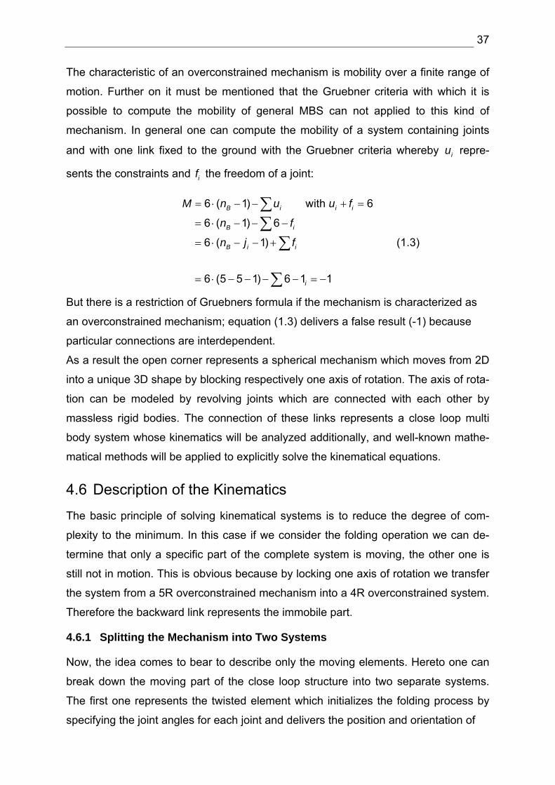
As a result the open corner represents a spherical mechanism which moves from 2D
into a unique 3D shape by blocking respectively one axis of rotation. The axis of rota-
tion can be modeled by revolving joints which are connected with each other by
massless rigid bodies. The connection of these links represents a close loop multi
body system whose kinematics will be analyzed additionally, and well-known mathe-
matical methods will be applied to explicitly solve the kinematical equations.
4.6 Description of the Kinematics
The basic principle of solving kinematical systems is to reduce the degree of com-
plexity to the minimum. In this case if we consider the folding operation we can de-
termine that only a specific part of the complete system is moving, the other one is
still not in motion. This is obvious because by locking one axis of rotation we transfer
the system from a 5R overconstrained mechanism into a 4R overconstrained system.
Therefore the backward link represents the immobile part.
4.6.1 Splitting the Mechanism into Two Systems
Now, the idea comes to bear to describe only the moving elements. Hereto one can
break down the moving part of the close loop structure into two separate systems.
The first one represents the twisted element which initializes the folding process by
specifying the joint angles for each joint and delivers the position and orientation of
38
Multi Close Loop System
Revolute Joint (R)Spherical Motion
Forward Kinematic Inverse Kinematic
End-Effector
Figure 4-10: How to model the kinematics
the end effector, a classical Forward Kinematic (FK) approach. The second part tries
to track the predetermined end effector position and represents an Inverse Kinematic
(IK) problem which is well known and already established in robotics, see Figure
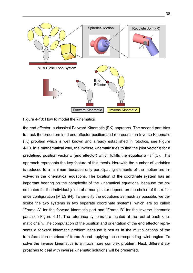
4-10. In a mathematical way, the inverse kinematic tries to find the joint vector q for a
predefined position vector x (end effector) which fulfills the equation 1( )q f x−= . This
approach represents the key feature of this thesis. Herewith the number of variables
is reduced to a minimum because only participating elements of the motion are in-
volved in the kinematical equations. The location of the coordinate system has an
important bearing on the complexity of the kinematical equations, because the co-
ordinates for the individual joints of a manipulator depend on the choice of the refer-
ence configuration [MrLS 94]. To simplify the equations as much as possible, we de-
scribe the two systems in two separate coordinate systems, which are so called
“Frame A” for the forward kinematic part and “Frame B” for the inverse kinematic
part, see Figure 4-11. The reference systems are located at the root of each kine-
matic chain. The computation of the position and orientation of the end effector repre-
sents a forward kinematic problem because it results in the multiplications of the
transformation matrices of frame A and applying the corresponding twist angles. To
solve the inverse kinematics is a much more complex problem. Next, different ap-
proaches to deal with inverse kinematic solutions will be presented.
39
Forward Kinematics Inverse Kinematics
end-effector
( )0 1
R dx
Θ⎛ ⎞= ⎜ ⎟⎝ ⎠
1q f (x)−=
User specifies joint angleComputer finds position of end-effector
User specifies end-effector positionComputer finds angles
( )0 1 11 2
0 1 11 1 2 2
( )
... ( )
( ) ( ) ... ( )
nn
n nn n
x f q
T T T x q
T q T q T q x
−
−
=
= ⋅ ⋅ ⋅
= ⋅ ⋅ ⋅
A B(0,0)
1Θ
2Θ
1l
2l
1l
2l3l
1Θ
2Θ
(0,0)
several solutions
3Θ
Figure 4-11: Splitting the system into a forward and inverse kinematic part
4.6.2 Solving the Inverse Kinematics
Inverse kinematics offers three ways how to get a solution. Possible methods are
algebraic, geometric and iterative. Algebraic and geometric methods provide an ex-
act solution and belong to the group of analytic solutions. If there are more solutions
then these methods provide all possible solutions. If the end-effector is inaccessible
then there is no solution available. Iterative methods offer a general solution of in-
verse kinematics and represent a numerical approach. Their disadvantage is that
they converge to only one solution even if there are several ones or they find a clos-
est solution if it doesn’t exist [Kang 00].
Geometric methods use the knowledge of the manipulator geometry. This method
bears the disadvantage that solutions for one manipulator cannot be transferred to a
manipulator with different geometry. In order to solve inverse kinematics with alge-
braic methods we need to solve equations for N degrees of freedom. Every joint
holds a transformation matrix iM that consists of a translational and rotational part,
both relative to its parents. The overall transformation is given by the product of the
matrices along the path from the base frame coordinate system to the end effector
by 1 2 1...i iM M M M M−= .
40
With the use of this matrix multiplication M the forward kinematics can be computed
in terms of the position and orientation of the end effector. The position and orienta-
tion of the end effector vector x in the parent's coordinate system is found by multi-
plying the position vector of the end effectorq , in its own coordinate system with the
transformation matrix M.
( )x f q= (1.4)
In contrast to that, the inverse kinematics is needed to compute the state vector q for
a given position and orientation of the end effector x which is the inverse function of
(1.4)
1( )q f x−= (1.5)
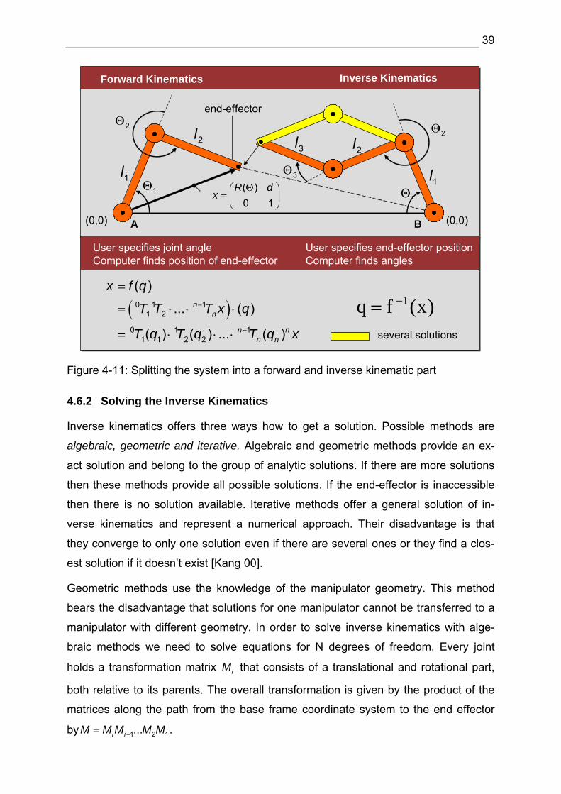
The solution of (1.5) is not simple because the function f is not linear and consisting
of terms of cosine and sine to describe the manipulator geometry. There is a one-
valued function for (1.4) but for (1.5) there are more solutions q for one x as illus-
trated in Figure 4-11.
Analytic Solution Numerical Solution
1 1cos( )a Θ 2 1 2cos( )a Θ +Θ x
y
1Θ
2Θ
1 1cos( )a Θ 2 1 2cos( )a Θ +Θ x
y
1Θ
2Θ
( )f Θ
x xδ+
goalx
( )goalf x
x
( )f Θ
x xδ+
goalx
( )goalf x
x
Iterate1( )J xδ δ−Θ = Θ
( )f δΘ + Θ
1 1
1 2
2 2
1 2
1 1 2 1 2 2 1 2
1 1 2 1 2 2 1 2
sin sin( ) sin( )cos cos( ) cos( )
f fx x
Jf fx x
a a aa a a
δ δδ δδ δδ δ
⎡ ⎤⎢ ⎥⎢ ⎥=⎢ ⎥⎢ ⎥⎣ ⎦− Θ − Θ +Θ − Θ +Θ⎡ ⎤
= ⎢ ⎥Θ + Θ +Θ Θ +Θ⎣ ⎦
1 1 1 2 1 2
1 1 1 2 1 2
( ) cos( ) cos( )( ) sin( ) sin( )
x f a ay f a a= Θ = Θ + Θ +Θ
= Θ = Θ + Θ +Θ
Equations can be solved analytically2 equations 2 variables
1 2... ...Θ = ∧ Θ =Solution
Figure 4-12: Two different solutions of the inverse kinematic equations
If the manipulator is changing its geometrical conformation, a numerical solution like
the iterative approach offers a nice opportunity to compute its inverse kinematics. An
Iterative solution is based on matrix inversion or on any form of optimization.
41
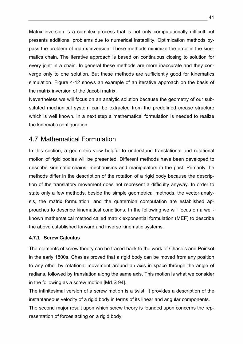
Matrix inversion is a complex process that is not only computationally difficult but
presents additional problems due to numerical instability. Optimization methods by-
pass the problem of matrix inversion. These methods minimize the error in the kine-
matics chain. The Iterative approach is based on continuous closing to solution for
every joint in a chain. In general these methods are more inaccurate and they con-
verge only to one solution. But these methods are sufficiently good for kinematics
simulation. Figure 4-12 shows an example of an iterative approach on the basis of
the matrix inversion of the Jacobi matrix.
Nevertheless we will focus on an analytic solution because the geometry of our sub-
stituted mechanical system can be extracted from the predefined crease structure
which is well known. In a next step a mathematical formulation is needed to realize
the kinematic configuration.
4.7 Mathematical Formulation
In this section, a geometric view helpful to understand translational and rotational
motion of rigid bodies will be presented. Different methods have been developed to
describe kinematic chains, mechanisms and manipulators in the past. Primarily the
methods differ in the description of the rotation of a rigid body because the descrip-
tion of the translatory movement does not represent a difficulty anyway. In order to
state only a few methods, beside the simple geometrical methods, the vector analy-
sis, the matrix formulation, and the quaternion computation are established ap-
proaches to describe kinematical conditions. In the following we will focus on a well-
known mathematical method called matrix exponential formulation (MEF) to describe
the above established forward and inverse kinematic systems.
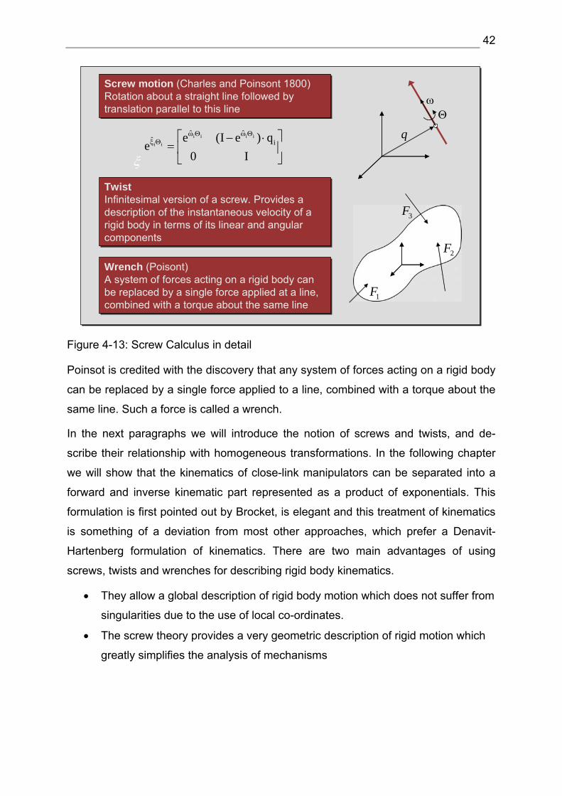
4.7.1 Screw Calculus
The elements of screw theory can be traced back to the work of Chasles and Poinsot
in the early 1800s. Chasles proved that a rigid body can be moved from any position
to any other by rotational movement around an axis in space through the angle of
radians, followed by translation along the same axis. This motion is what we consider
in the following as a screw motion [MrLS 94].
The infinitesimal version of a screw motion is a twist. It provides a description of the
instantaneous velocity of a rigid body in terms of its linear and angular components.
The second major result upon which screw theory is founded upon concerns the rep-
resentation of forces acting on a rigid body.
42
Screw motion (Charles and Poinsont 1800)Rotation about a straight line followed by translation parallel to this line
Screw motion (Charles and Poinsont 1800)Rotation about a straight line followed by translation parallel to this line
TwistInfinitesimal version of a screw. Provides a description of the instantaneous velocity of a rigid body in terms of its linear and angular components
TwistInfinitesimal version of a screw. Provides a description of the instantaneous velocity of a rigid body in terms of its linear and angular components
Wrench (Poisont)A system of forces acting on a rigid body can be replaced by a single force applied at a line, combined with a torque about the same line
Wrench (Poisont)A system of forces acting on a rigid body can be replaced by a single force applied at a line, combined with a torque about the same line
1F
2F
3F
q
ω
ξ
Θ
i i i ii i
ˆ ˆˆ ie (I e ) q
e0 I
ω Θ ωΘξ Θ ⎡ ⎤− ⋅
= ⎢ ⎥⎣ ⎦
Figure 4-13: Screw Calculus in detail
Poinsot is credited with the discovery that any system of forces acting on a rigid body
can be replaced by a single force applied to a line, combined with a torque about the
same line. Such a force is called a wrench.
In the next paragraphs we will introduce the notion of screws and twists, and de-
scribe their relationship with homogeneous transformations. In the following chapter
we will show that the kinematics of close-link manipulators can be separated into a
forward and inverse kinematic part represented as a product of exponentials. This
formulation is first pointed out by Brocket, is elegant and this treatment of kinematics
is something of a deviation from most other approaches, which prefer a Denavit-
Hartenberg formulation of kinematics. There are two main advantages of using
screws, twists and wrenches for describing rigid body kinematics.
• They allow a global description of rigid body motion which does not suffer from
singularities due to the use of local co-ordinates.
• The screw theory provides a very geometric description of rigid motion which
greatly simplifies the analysis of mechanisms
43
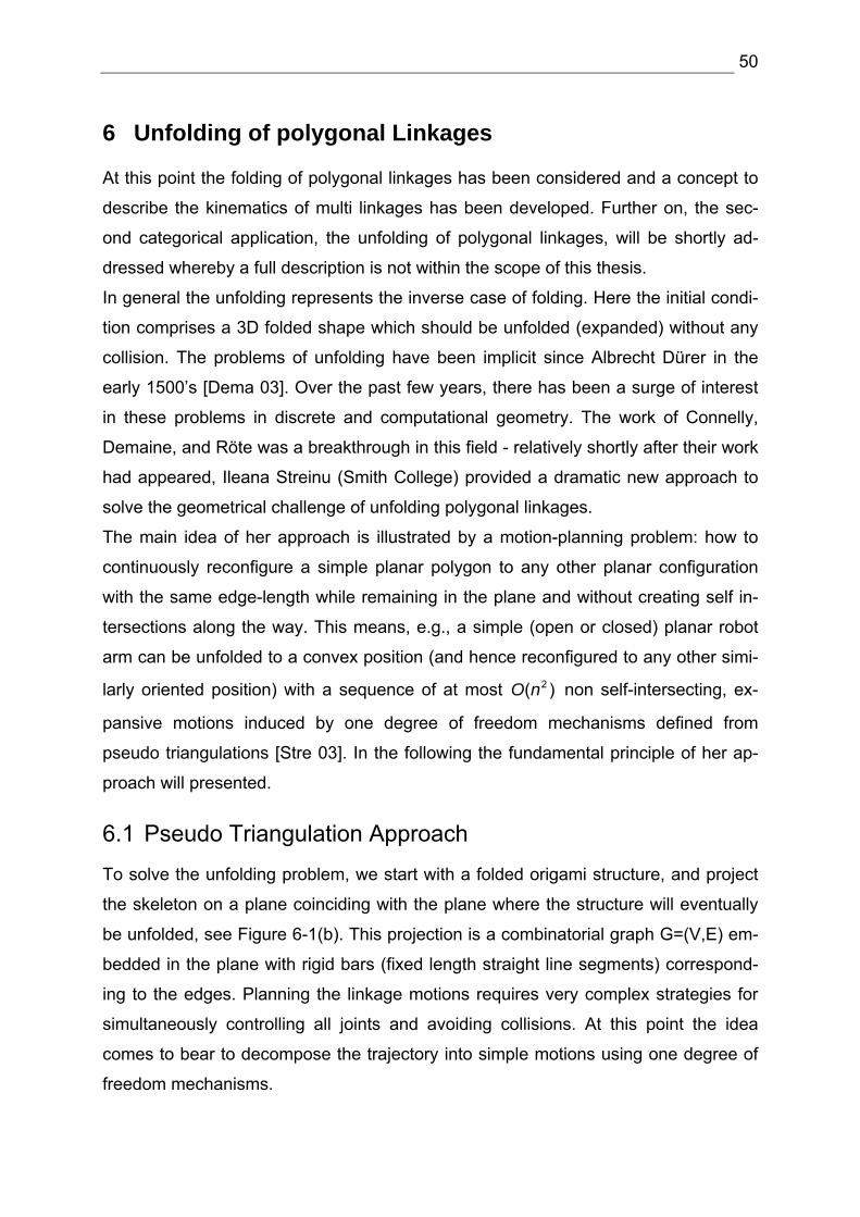
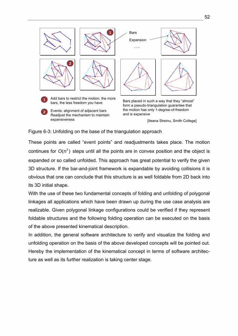
5 Folding of Polygonal Linkages
All requirements to start describing the folding of polygonal linkages are set. The
topological and kinematical classification is presented as well as a mathematical for-
mulation in terms of the exponential matrix formulations is defined. In a next step the
above developed concept, to apply a substituted mechanical system to a paper fold-
ing model, will be reconstructed in detail on a demonstration model.
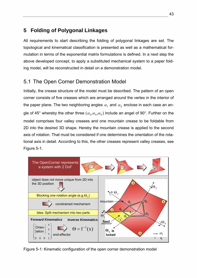
5.1 The Open Corner Demonstration Model
Initially, the crease structure of the model must be described. The pattern of an open
corner consists of five creases which are arranged around the vertex in the interior of
the paper plane. The two neighboring angles 1α and 2α enclose in each case an an-
gle of 45° whereby the other three ( 3 4 5, ,α α α ) include an angel of 90°. Further on the
model comprises four valley creases and one mountain crease to be foldable from
2D into the desired 3D shape. Hereby the mountain crease is applied to the second
axis of rotation. That must be considered if one determines the orientation of the rota-
tional axis in detail. According to this, the other creases represent valley creases, see
Figure 5-1.
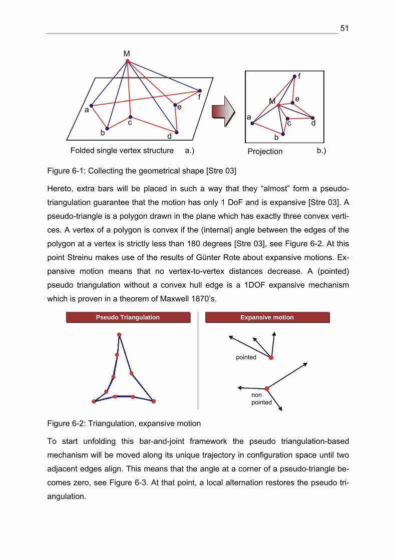
The OpenCorner represents a system with 2 DoF
object does not move unique from 2D into the 3D position
constrained mechanism
Blocking one rotation angle (e.g. )
Idea: Split mechanism into two parts
Forward Kinematics Inverse Kinematics
end-effector
xyz
0 0 0 1
⎛ ⎞⎜ ⎟⎜ ⎟⎜ ⎟⎜ ⎟⎜ ⎟⎝ ⎠
1f (x)−Θ =
3Θ
4Θ1Θ
2Θ
5Θ is locked
5Θ is locked
5Θ
Orien-tation
⎛ ⎞⎜ ⎟⎜ ⎟⎜ ⎟⎝ ⎠
fixedfixed
iωiq
mountain
1q
2q 3q
4q5q
1α
1
2
3
4
5
Figure 5-1: Kinematic configuration of the open corner demonstration model
44
After the crease structure is defined, the substituted mechanical system can be ap-
plied. As mentioned in chapter 4 the spherical movement will be modeled by revolute
joints which are connected with rigid bodies around the vertex. Therefore each
crease line will be replaced with a revolute joint consisting of a line item specification
in respect to its corresponding reference system and an orientation with regard to the
rotational direction (mountain or valley crease). Among each other, all joints are con-
nected by bodies to form a close loop structure, see Figure 5-1.
Transferred to the exponential matrix notation this means that each joint is character-
ized by the point nq , where the axis of rotation is going through and the unit vector iω
in the direction of the twist axis. Hereby the joint vectors nq are pointing from the cor-
responding reference system to the joints. In the first instance, all joint vectors will be
described in reference to a base co-ordinate system in the interior of the plane. If all
creases are replaced by joints and described with the use of the two parameters nq
and iω , the actual description of the folding operation can be as follows.
Similar to the paper folding model, where one holds a fragment stationary, and fold
the rest of the paper flat along the proposed crease line, one body (1) will be con-
nected to the ground. Hereupon two possible axes of rotation 1 2( , )Θ Θ to initialize the
folding operation come to bear, see Figure 5-1.
Spherical motion from 2D into 3D
1Θ
2Θ
3Θ
4Θ
Frame AFrame A
Frame BFrame B
End-EffectorInverse Kinematics (IK)
Forward Kinematics (FK)
modeled with revolute joints
d
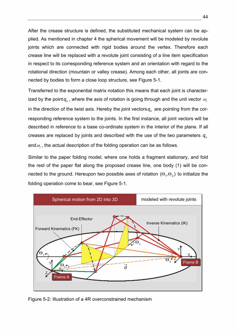
Figure 5-2: Illustration of a 4R overconstrained mechanism
45
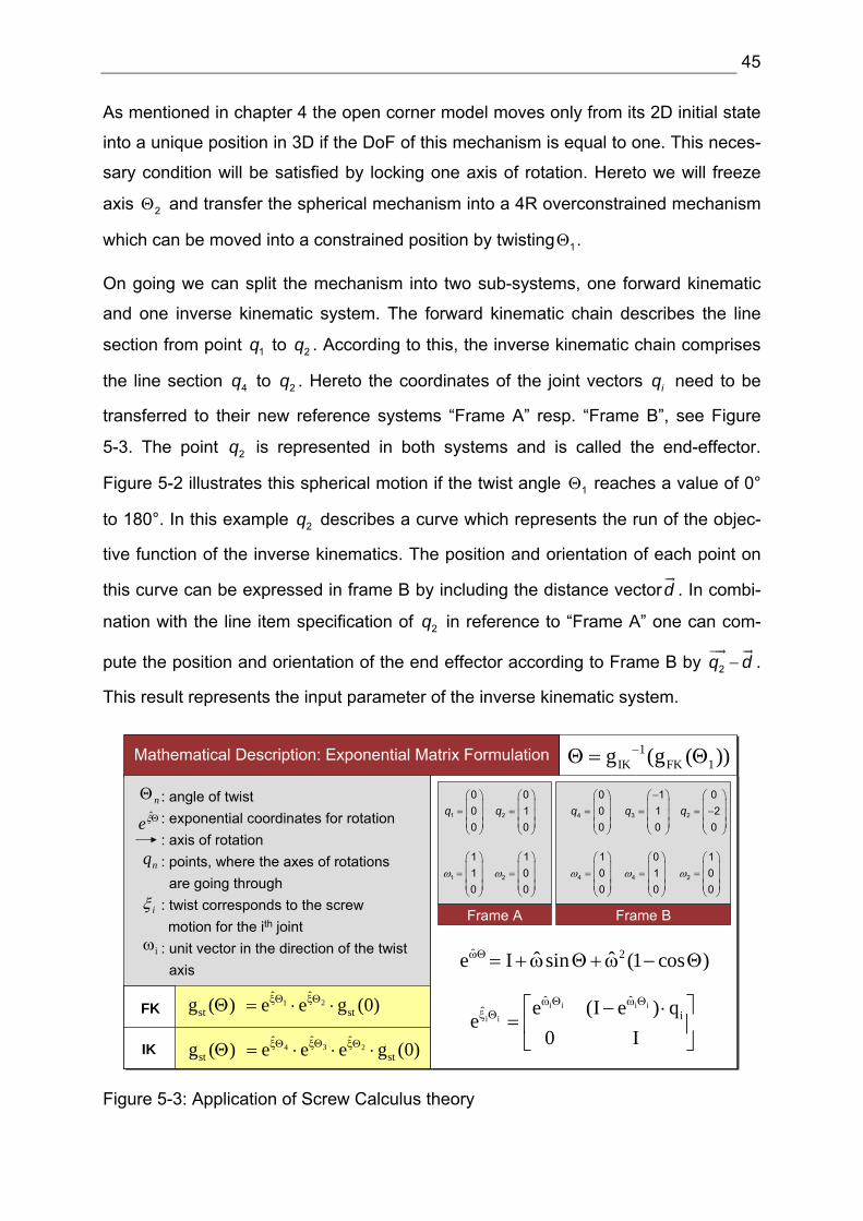
As mentioned in chapter 4 the open corner model moves only from its 2D initial state
into a unique position in 3D if the DoF of this mechanism is equal to one. This neces-
sary condition will be satisfied by locking one axis of rotation. Hereto we will freeze
axis 2Θ and transfer the spherical mechanism into a 4R overconstrained mechanism
which can be moved into a constrained position by twisting 1Θ .
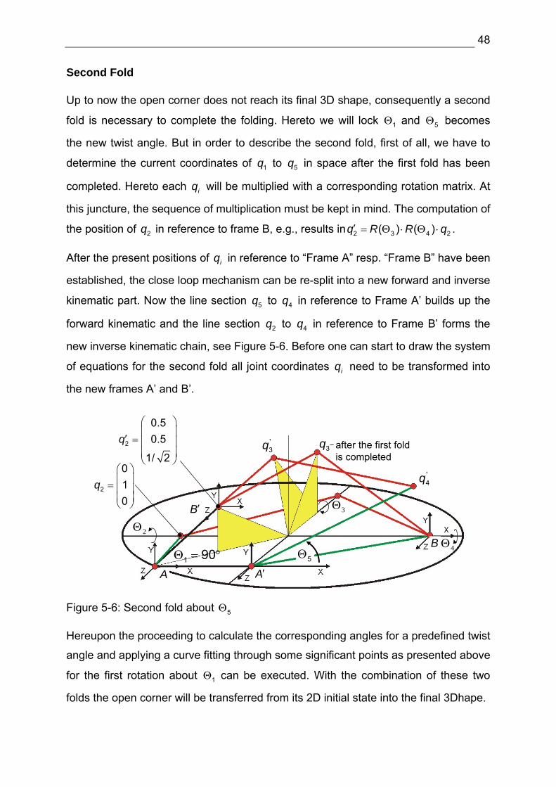
On going we can split the mechanism into two sub-systems, one forward kinematic
and one inverse kinematic system. The forward kinematic chain describes the line
section from point 1q to 2q . According to this, the inverse kinematic chain comprises
the line section 4q to 2q . Hereto the coordinates of the joint vectors iq need to be
transferred to their new reference systems “Frame A” resp. “Frame B”, see Figure
5-3. The point 2q is represented in both systems and is called the end-effector.
Figure 5-2 illustrates this spherical motion if the twist angle 1Θ reaches a value of 0°
to 180°. In this example 2q describes a curve which represents the run of the objec-
tive function of the inverse kinematics. The position and orientation of each point on
this curve can be expressed in frame B by including the distance vectord . In combi-
nation with the line item specification of 2q in reference to “Frame A” one can com-
pute the position and orientation of the end effector according to Frame B by 2q d− .
This result represents the input parameter of the inverse kinematic system.
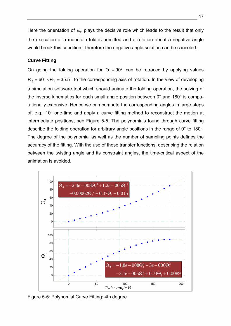
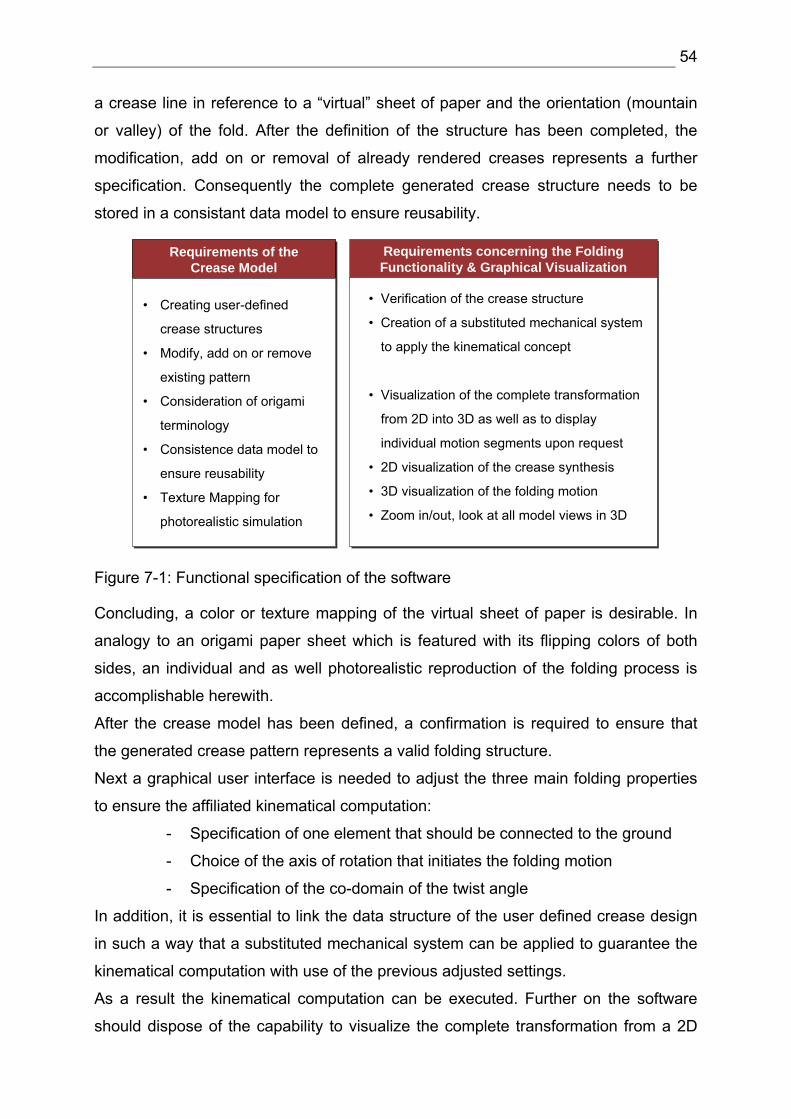
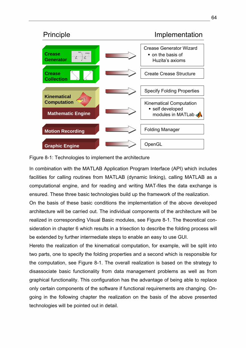
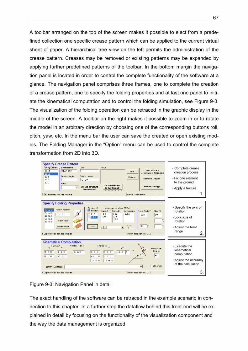
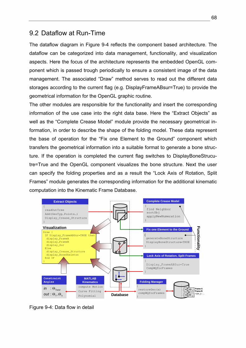
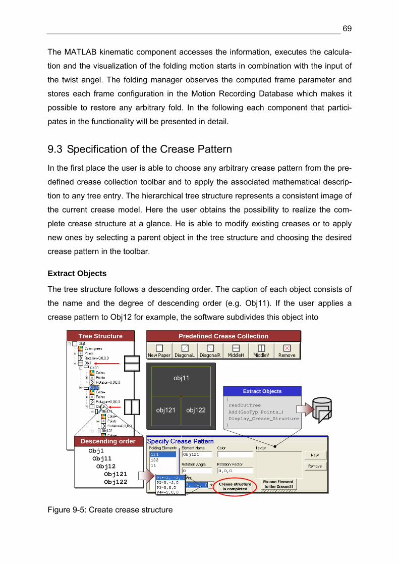
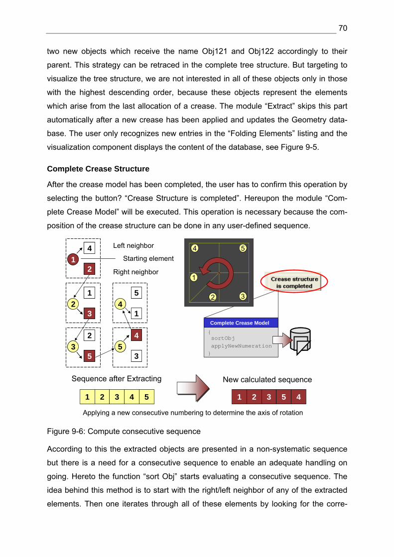
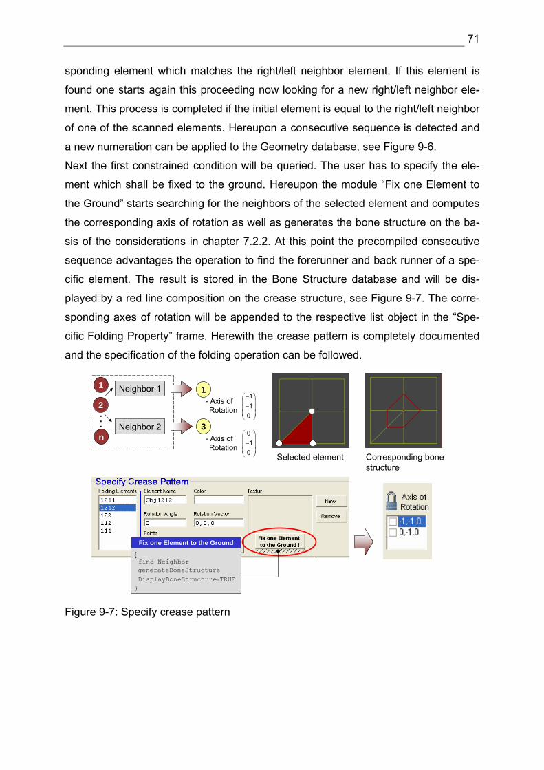
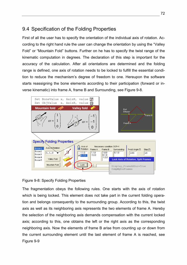
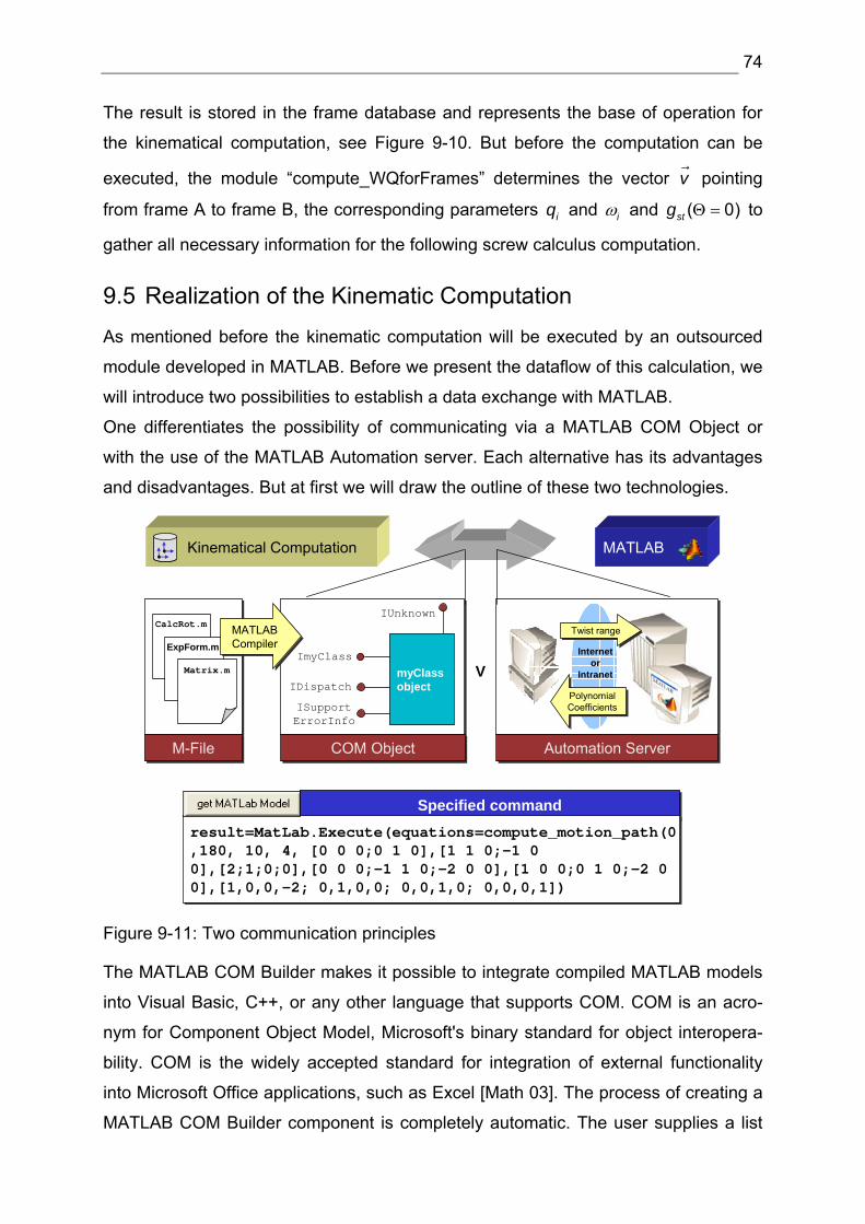
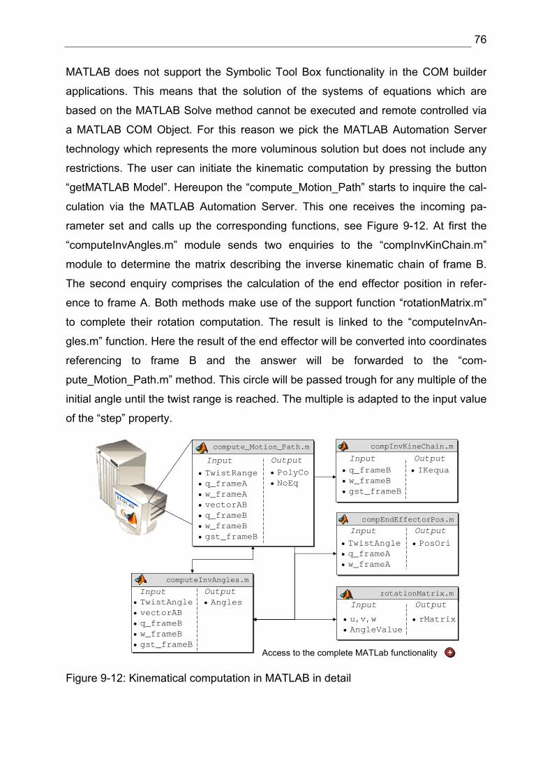
9.6 Graphical Visualization with the use of OpenGL
The visualization architecture of the folding process is directed to the functional prin-
ciple of OpenGL. OpenGL is a software interface to graphic hardware. This interface
consists of 250 distinct commands to specify the objects and operations to produce
interactive 3D applications. OpenGL is designed as a streamlined, hardware-
independent interface to be implemented on many different hardware platforms
[WND+ 99]. One of the most important characteristics of OpenGL is that it does not
provide high-level commands for describing models of 3D objects. This means the
development of a graphic model is built up from a small set of geometric primitives –
points, lines and polygons that are specified by their vertices.
In order to render a graphic scene consisting of a number of polygons, its object co-
ordinates need to be determined/computed first. The object coordinates comprise the
points that describe the shape of the model in 3D space. In order to draw these ob-
jects on a flat 2D computer screen, an additional transformation of these coordinates
into 2D screen coordinates is required. This proceeding is executed in the so called
OpenGL Geometric Pipeline and is illustrated ongoing. First of all we will focus on the
creation of the object coordinates of our folding model.
In order to display the geometrical shape of a folding model, we primarily make use
of the two primitive geometric objects, a triangle and a quadrilateral polygon. A com-
position of these objects builds up the folding model. The necessary information de-
scribing their shape will be delivered as a dataset of the Kinematic Frame database.
The rotation angle of each element relative to its forerunner or back runner is as well
known in terms of the twist angle and the computed constraint angles for each point
of time during the folding operation.
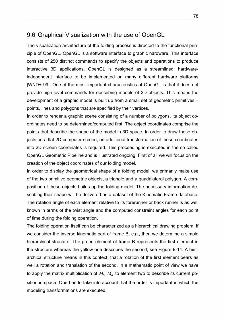
The folding operation itself can be characterized as a hierarchical drawing problem. If
we consider the inverse kinematic part of frame B, e.g., then we determine a simple
hierarchical structure. The green element of frame B represents the first element in
the structure whereas the yellow one describes the second, see Figure 9-14. A hier-
archical structure means in this context, that a rotation of the first element bears as
well a rotation and translation of the second. In a mathematic point of view we have
to apply the matrix multiplication of 3 4M M⋅ to element two to describe its current po-
sition in space. One has to take into account that the order is important in which the
modeling transformations are executed.
79
This matrix multiplication is implemented in OpenGL by using a matrix stack. A matrix
stack is an efficient way to track matrices while traversing a transform hierarchy [Con
03]. This is particularly useful when you are drawing complicated objects that are
built up from simpler ones as well as to save and restore certain transformations.
At any point in a drawing, there is a current matrix on top of the matrix stack, com-
posed of all transformations thus far. In this particular example the matrix transforma-
tion M4 will be set to the first current matrix stack. The current matrix stack (M4) will
be defined with the OpenGL command pushMatrix and canceled with the according
popMatrix order. All geometrical transformations between these two operations will
be executed in reference to the current matrix stack (M4). This technique allows to
determine the object coordinates of each element of the folding model in 3D space
by applying the precompiled angle positions to the corresponding matrix stack.
ConstraintAngles
1 n
: : ..
Twistinout
Θ
Θ Θ
ConstraintAngles
1 n
: : ..
Twistinout
Θ
Θ Θ
Draw IF Display_FrameABSur=TRUE thendisplay_FrameAdisplay_FrameBdisplay_SurElsedisplay_Crease_Structuredisplay_BoneSkeletonEnd IF
Draw IF Display_FrameABSur=TRUE thendisplay_FrameAdisplay_FrameBdisplay_SurElsedisplay_Crease_Structuredisplay_BoneSkeletonEnd IF
Display FrameB glPushMatrixFor x=1 to NoObjglRotate( ,x,y,z)glBegin Obj(x)glVertex x,y,z…glEndNext x
glPopMatrix
Obj 4
Obj 3
4M
3M
3 4M M⋅
Obj 2 Obj 1
Obj 5
Frame A Frame B Surrounding
1M
Hierarchical representation of the Matrix Stack
Θ4M
3M
Ope
nGL
⎥⎥⎥⎥
⎦
⎤
⎢⎢⎢⎢
⎣
⎡
wzyx
Objectcoordinates
1M
Figure 9-14: Computing the object coordinates
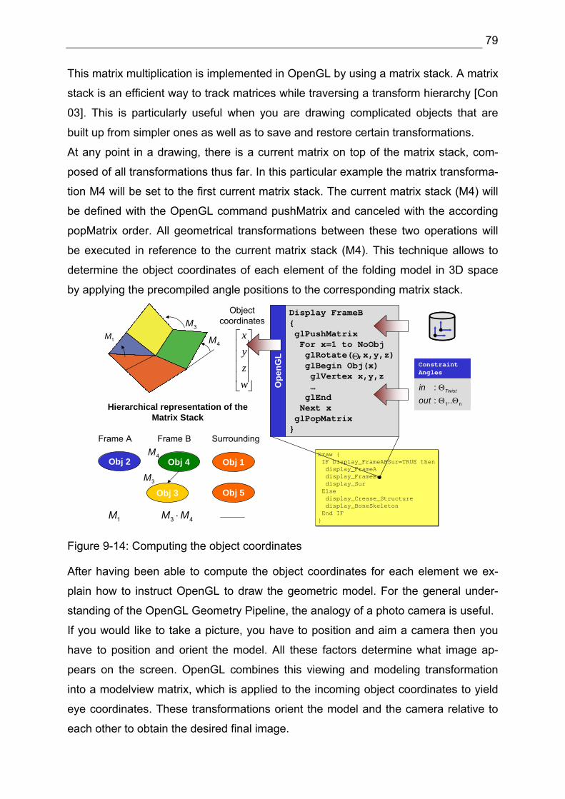
After having been able to compute the object coordinates for each element we ex-
plain how to instruct OpenGL to draw the geometric model. For the general under-
standing of the OpenGL Geometry Pipeline, the analogy of a photo camera is useful.
If you would like to take a picture, you have to position and aim a camera then you
have to position and orient the model. All these factors determine what image ap-
pears on the screen. OpenGL combines this viewing and modeling transformation
into a modelview matrix, which is applied to the incoming object coordinates to yield
eye coordinates. These transformations orient the model and the camera relative to
each other to obtain the desired final image.
80
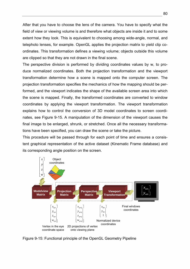
After that you have to choose the lens of the camera. You have to specify what the
field of view or viewing volume is and therefore what objects are inside it and to some
extent how they look. This is equivalent to choosing among wide-angle, normal, and
telephoto lenses, for example. OpenGL applies the projection matrix to yield clip co-
ordinates. This transformation defines a viewing volume; objects outside this volume
are clipped so that they are not drawn in the final scene.
The perspective division is performed by dividing coordinates values by w, to pro-
duce normalized coordinates. Both the projection transformation and the viewport
transformation determine how a scene is mapped onto the computer screen. The
projection transformation specifies the mechanics of how the mapping should be per-
formed, and the viewport indicates the shape of the available screen area into which
the scene is mapped. Finally, the transformed coordinates are converted to window
coordinates by applying the viewport transformation. The viewport transformation
explains how to control the conversion of 3D model coordinates to screen coordi-
nates, see Figure 9-15. A manipulation of the dimension of the viewport causes the
final image to be enlarged, shrunk, or stretched. Once all the necessary transforma-
tions have been specified, you can draw the scene or take the picture.
This procedure will be passed through for each point of time and ensures a consis-
tent graphical representation of the active dataset (Kinematic Frame database) and
its corresponding angle position on the screen.
Objectcoordinates
⎥⎥⎥⎥
⎦
⎤
⎢⎢⎢⎢
⎣
⎡
wzyx
Vertex in the eye coordinate space
2D projections of vertex onto viewing plane
⎥⎥⎥⎥⎥
⎦
⎤
⎢⎢⎢⎢⎢
⎣
⎡
eye
eye
eye
eye
wzyx
⎥⎥⎥⎥⎥
⎦
⎤
⎢⎢⎢⎢⎢
⎣
⎡
proj
proj
proj
proj
wzyx
⎥⎥⎥
⎦
⎤
⎢⎢⎢
⎣
⎡
1dev
dev
yx
Normalized device coordinates
Final windowscoordinates
ProjectionMatrix
PerspectiveMatrix
ModelviewMatrix
ViewportTransformation
win
win
xy⎡ ⎤⎢ ⎥⎣ ⎦
Figure 9-15: Functional principle of the OpenGL Geometry Pipeline
81
9.7 Realization of the Folding Manager
So far the implementation of the visualization of one fold is completed. As mentioned
before, to ensure the transformation from a 2D initial state into the desired 3D shape
we are interestied in displaying several folds in a row resp. to repeat selective sec-
tions of one fold upon request. This required functional specification is implemented
in the Folding Manager.
The Folding Manager can be addressed in the menu “Option”. After the first fold has
been completed, the user presses the button “StoreCurrentGeometry” and generates
a new starting position to trigger any other fold. The procedure “restoreGeo” calcu-
lates the current position of each element participating in the folding in 3D space.
Further on it stores the new position in the Geometry database and generates on the
basis of this data a new bone structure frame, see Figure 9-16. Hereto the position of
each point of the folding model needs be multiplied with a corresponding transforma-
tion matrix which describes its current position in space. In order to compute the ma-
trix multiplication we make use of a self developed MATLAB COM Object, the so
called Transformation library which provides the function “computeRotatedPoint” to
the “restoreGeo” procedure of the Visual Basic host application.
5Θ
0 180°→ °0 90°→ °2 Folds
1Θ
Folding ManagerrestoreGeo(x)compWQforFrames
Folding ManagerrestoreGeo(x)compWQforFrames
Frame A1Θ
( )1 ...f Θ =nΘ
Frame BFrame A
1Θ( )1 ...f Θ =
nΘFrame B
Figure 9-16: Functional principle of the Folding Manager
82
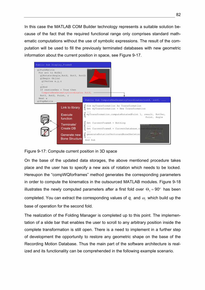
In this case the MATLAB COM Builder technology represents a suitable solution be-
cause of the fact that the required functional range only comprises standard math-
ematic computations without the use of symbolic expressions. The result of the com-
putation will be used to fill the previously terminated databases with new geometric
information about the current position in space, see Figure 9-17.
Public Sub Display_FrameBPublic Sub Display_FrameB
glPushMatrixFor x=1 to NoObjglRotate(Angle,RotX, RotY, RotZ)glBegin Obj(x)glVertex x,y,z…glEndIf restoreGeo = True then ComputeNewGeometryCoordinates RotX,RotY, RotZ, Point, r
Next xglPopMatrix
glPushMatrixFor x=1 to NoObjglRotate(Angle,RotX, RotY, RotZ)glBegin Obj(x)glVertex x,y,z…glEndIf restoreGeo = True then ComputeNewGeometryCoordinates RotX,RotY, RotZ, Point, r
Next xglPopMatrix Public Sub ComputeNewGeometryCoordinates(rotX, rotY, ...
Dim myTransformation As TransformationSet myTransformation = New Transformation ...myTransformation.computeRotatedPoint 1, result, RotVec,
Point, Angle
Set CurrentFrameA = Nothing...Set CurrentFrameA = CurrentDatabase.createSurrounding...generateRotationVectorandBoneSkeleton...End Sub
Generate new Bone Structure
Terminate/ Create DB
Execute function
Link to library
Figure 9-17: Compute current position in 3D space
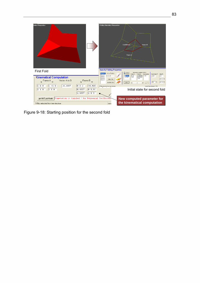
On the base of the updated data storages, the above mentioned procedure takes
place and the user has to specify a new axis of rotation which needs to be locked.
Hereupon the “compWQforframes” method generates the corresponding parameters
in order to compute the kinematics in the outsourced MATLAB modules. Figure 9-18
illustrates the newly computed parameters after a first fold over 1 90Θ = ° has been
completed. You can extract the corresponding values of iq and iω which build up the
base of operation for the second fold.
The realization of the Folding Manager is completed up to this point. The implemen-
tation of a slide bar that enables the user to scroll to any arbitrary position inside the
complete transformation is still open. There is a need to implement in a further step
of development the opportunity to restore any geometric shape on the base of the
Recording Motion Database. Thus the main part of the software architecture is real-
ized and its functionality can be comprehended in the following example scenario.
83
First Fold
Initial state for second fold
New computed parameter for the kinematical computationNew computed parameter for the kinematical computation
Figure 9-18: Starting position for the second fold
84
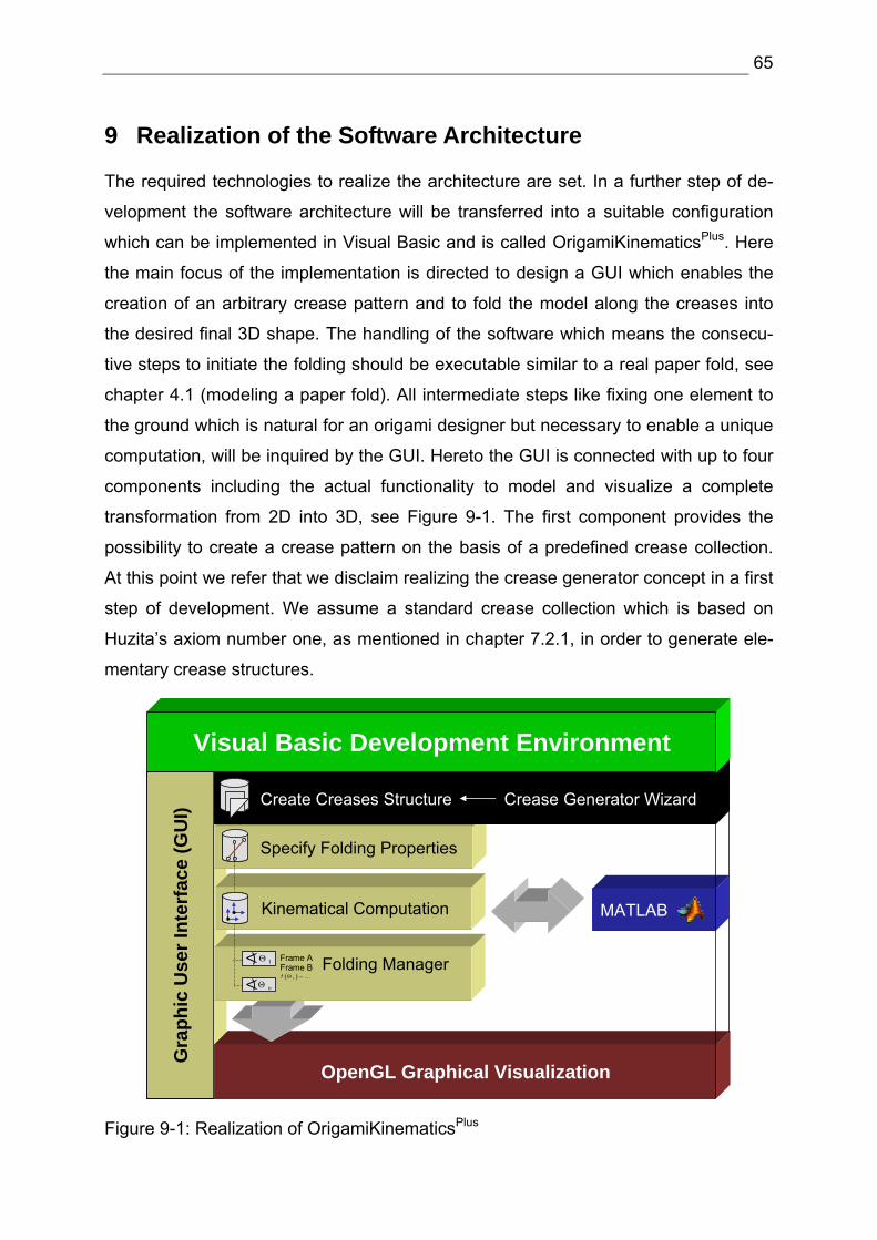
10 Example Scenario
Concluding, the functionality of the software package will be illustrated in an example
scenario. The scenario comprises three steps and describes the simulation of an
open corner getting folded from its 2D initial state into the intended 3D shape.
At first the creation of the corresponding crease structure will be addressed shortly.
Next we will discuss a particular case and try to fold an invalid crease structure. Si-
multaneously, possibilities will be presented in order to deal with this special configu-
ration. On the base of a valid crease pattern the complete transformation of the dem-
onstration model will be pointed out in detail. This operation is illustrated in terms of
the result of the mathematical computation as well as in screen shots visualizing the
transformation. At last the multifariousness of the graphic rendering will be demon-
strated.
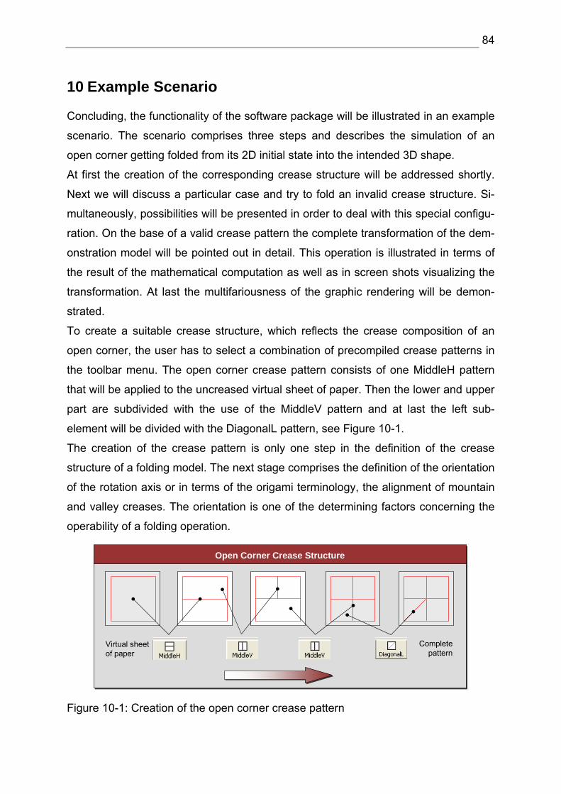
To create a suitable crease structure, which reflects the crease composition of an
open corner, the user has to select a combination of precompiled crease patterns in
the toolbar menu. The open corner crease pattern consists of one MiddleH pattern
that will be applied to the uncreased virtual sheet of paper. Then the lower and upper
part are subdivided with the use of the MiddleV pattern and at last the left sub-
element will be divided with the DiagonalL pattern, see Figure 10-1.
The creation of the crease pattern is only one step in the definition of the crease
structure of a folding model. The next stage comprises the definition of the orientation
of the rotation axis or in terms of the origami terminology, the alignment of mountain
and valley creases. The orientation is one of the determining factors concerning the
operability of a folding operation.
Open Corner Crease StructureOpen Corner Crease Structure
Virtual sheet of paper
Complete pattern
Figure 10-1: Creation of the open corner crease pattern
85
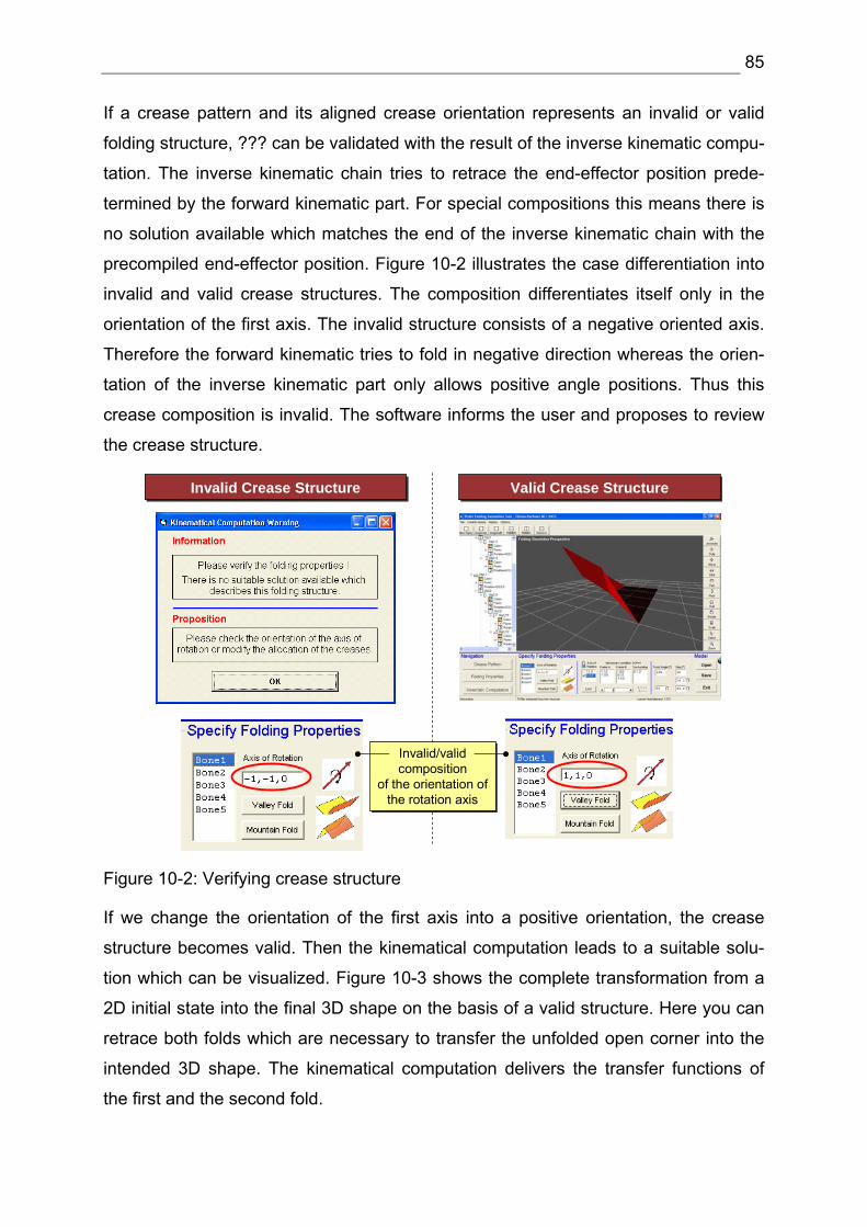
If a crease pattern and its aligned crease orientation represents an invalid or valid
folding structure, ??? can be validated with the result of the inverse kinematic compu-
tation. The inverse kinematic chain tries to retrace the end-effector position prede-
termined by the forward kinematic part. For special compositions this means there is
no solution available which matches the end of the inverse kinematic chain with the
precompiled end-effector position. Figure 10-2 illustrates the case differentiation into
invalid and valid crease structures. The composition differentiates itself only in the
orientation of the first axis. The invalid structure consists of a negative oriented axis.
Therefore the forward kinematic tries to fold in negative direction whereas the orien-
tation of the inverse kinematic part only allows positive angle positions. Thus this
crease composition is invalid. The software informs the user and proposes to review
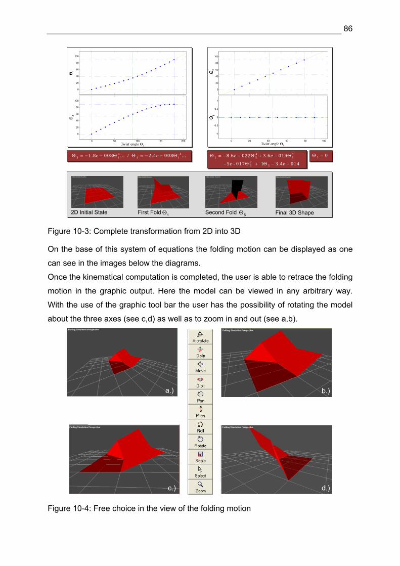
Final 3D Shape2D Initial State First Fold Second Fold1Θ 5Θ
Figure 10-3: Complete transformation from 2D into 3D
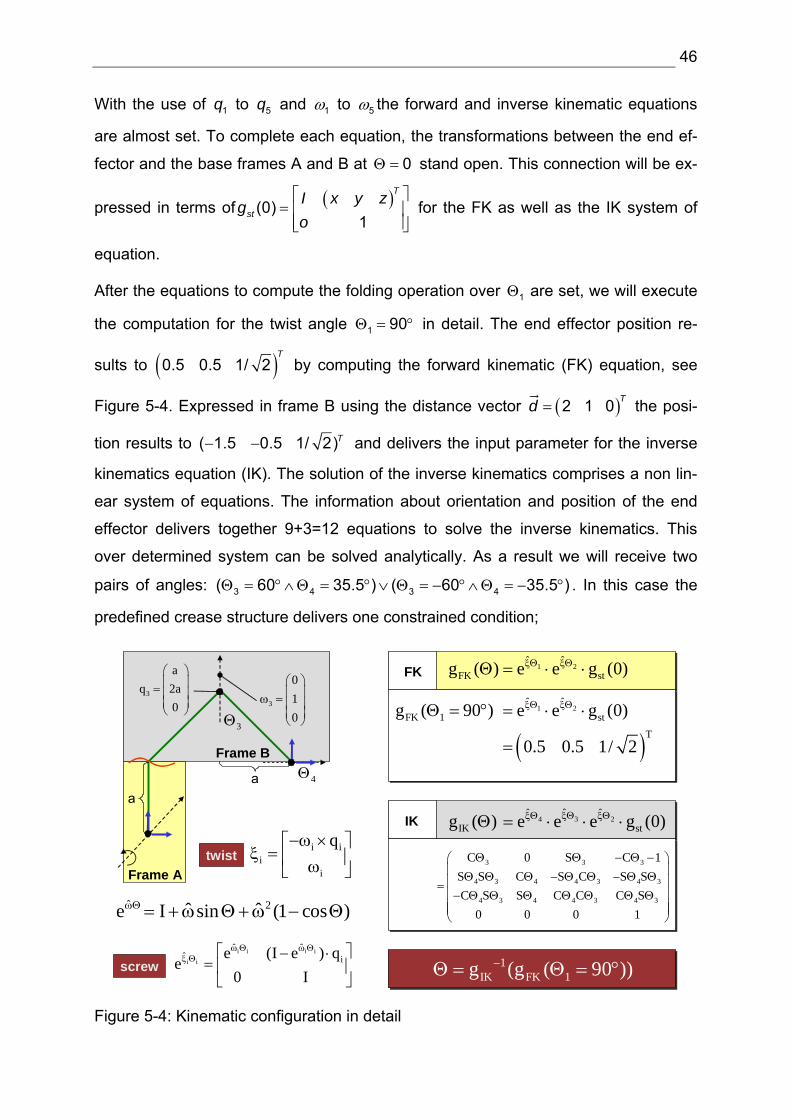
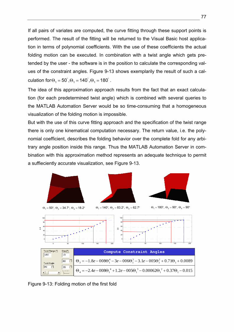
On the base of this system of equations the folding motion can be displayed as one
can see in the images below the diagrams.
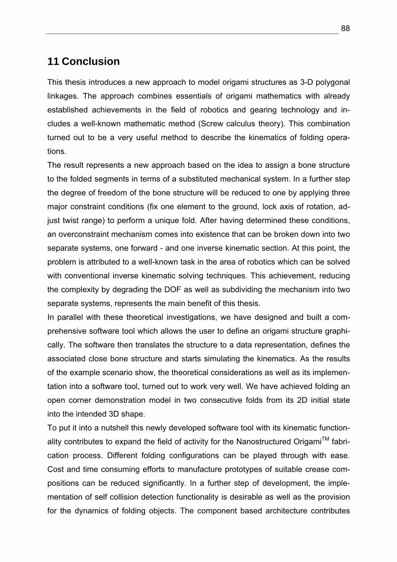
Once the kinematical computation is completed, the user is able to retrace the folding
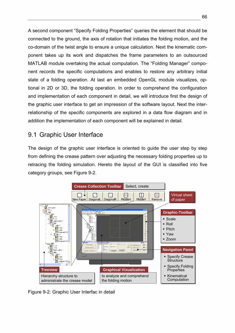
motion in the graphic output. Here the model can be viewed in any arbitrary way.
With the use of the graphic tool bar the user has the possibility of rotating the model
about the three axes (see c,d) as well as to zoom in and out (see a,b).
a.) b.)
c.) d.)
Figure 10-4: Free choice in the view of the folding motion
87
The opportunity to observe the model from all sides, from the top, from behind or
from the bottom of the model, supports the comprehension of the folding motion. Es-
pecially concerning typical engineering tasks, this photorealistic visualization contrib-
utes to retrace the construction. Finally, the fading of a grid relieves the orientation in
3D space by rotating the model.
88
11 Conclusion
This thesis introduces a new approach to model origami structures as 3-D polygonal
linkages. The approach combines essentials of origami mathematics with already
established achievements in the field of robotics and gearing technology and in-
cludes a well-known mathematic method (Screw calculus theory). This combination
turned out to be a very useful method to describe the kinematics of folding opera-
tions.
The result represents a new approach based on the idea to assign a bone structure
to the folded segments in terms of a substituted mechanical system. In a further step
the degree of freedom of the bone structure will be reduced to one by applying three
major constraint conditions (fix one element to the ground, lock axis of rotation, ad-
just twist range) to perform a unique fold. After having determined these conditions,
an overconstraint mechanism comes into existence that can be broken down into two
separate systems, one forward - and one inverse kinematic section. At this point, the
problem is attributed to a well-known task in the area of robotics which can be solved
with conventional inverse kinematic solving techniques. This achievement, reducing
the complexity by degrading the DOF as well as subdividing the mechanism into two
separate systems, represents the main benefit of this thesis.
In parallel with these theoretical investigations, we have designed and built a com-
prehensive software tool which allows the user to define an origami structure graphi-
cally. The software then translates the structure to a data representation, defines the
associated close bone structure and starts simulating the kinematics. As the results
of the example scenario show, the theoretical considerations as well as its implemen-
tation into a software tool, turned out to work very well. We have achieved folding an
open corner demonstration model in two consecutive folds from its 2D initial state
into the intended 3D shape.
To put it into a nutshell this newly developed software tool with its kinematic function-
ality contributes to expand the field of activity for the Nanostructured OrigamiTM fabri-
cation process. Different folding configurations can be played through with ease.
Cost and time consuming efforts to manufacture prototypes of suitable crease com-
positions can be reduced significantly. In a further step of development, the imple-
mentation of self collision detection functionality is desirable as well as the provision
for the dynamics of folding objects. The component based architecture contributes
89
outstandingly to this development. Completing the functionality range, it is of major
interest to include the inverse case in future which means the unfolding of polygonal
linkages by implementing Ileana Streinu’s pseudo triangulation approach.
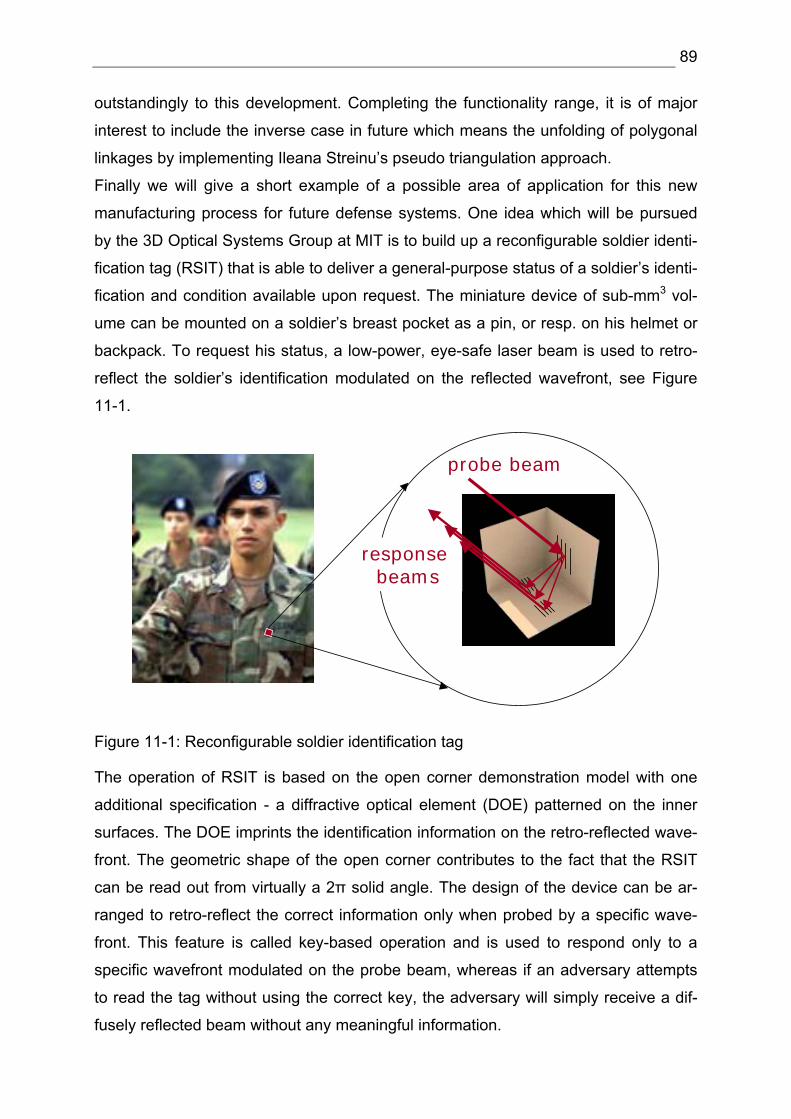
Finally we will give a short example of a possible area of application for this new
manufacturing process for future defense systems. One idea which will be pursued
by the 3D Optical Systems Group at MIT is to build up a reconfigurable soldier identi-
fication tag (RSIT) that is able to deliver a general-purpose status of a soldier’s identi-
fication and condition available upon request. The miniature device of sub-mm3 vol-
ume can be mounted on a soldier’s breast pocket as a pin, or resp. on his helmet or
backpack. To request his status, a low-power, eye-safe laser beam is used to retro-
reflect the soldier’s identification modulated on the reflected wavefront, see Figure
11-1.
probe beam
response beams
Figure 11-1: Reconfigurable soldier identification tag
The operation of RSIT is based on the open corner demonstration model with one
additional specification - a diffractive optical element (DOE) patterned on the inner
surfaces. The DOE imprints the identification information on the retro-reflected wave-
front. The geometric shape of the open corner contributes to the fact that the RSIT
can be read out from virtually a 2π solid angle. The design of the device can be ar-
ranged to retro-reflect the correct information only when probed by a specific wave-
front. This feature is called key-based operation and is used to respond only to a
specific wavefront modulated on the probe beam, whereas if an adversary attempts
to read the tag without using the correct key, the adversary will simply receive a dif-
fusely reflected beam without any meaningful information.
90
For this purpose, the DOEs are patterned via lithography on the flat surfaces during
the 1st step of the Nanostructured OrigamiTM process. In a second step of manufac-
turing, the RSIT folds itself into the intended position which results in high yield and
low cost. This feature enables as well the reconfigurability during the operation. This
means that the RSIT can fold itself to change its operation, e.g., to flip itself around to
retro-reflect confusing information to adversaries.
This example illustrates outstandingly the technological benefit of the Nanostructured
OrigamiTM technology. The determining factor of this application is the folding mecha-
nism. Other by folding, gratings cannot be fabricated on “vertical” walls with conven-
tional lithography! To obtain a retro-reflector with DOE, as shown in Figure 11-1, the
only other alternative would be to manually assemble discrete elements, which would
be expensive and prone to inaccuracies and low yield. Thus, the Nanostructured Ori-
gamiTM technology in combination with the presented achievements concerning the
folding of polygonal linkage opens up new vistas for a wide range of future applica-
tions in both military as well as commercial arenas [Bar 03].
91
12 Abbreviations
2D Two Dimensional
3D Three Dimensional
API Application Interface
CC Crease Collection
CG Crease Generator
COM Component Object Model
DARPA Defense Advanced Research Projects Agency
DB Database
DNA Deoxyribonucleic Acid
DOE Diffractive Optical Element
DOF Degree of Freedom
FK Forward Kinematic
GUI Graphic User Interface
ID Identification Code
IK Inverse Kinematic
MATLAB Matrix Laboratory
MBS Multi Body System
MCLS Multi Close Loop System
MEF Matrix Exponential Formulation
MEMS Micro Electro Mechanical System
MIT Massachusetts Institute of Technology
RSIT Reconfigurable Soldier Identification Tag
TTS Tree Type System
VLSI Very Large Scale Integrator
92
13 References
[AmSo 00] Amato, N.; Song, G.: Motion Planning Approach to Folding: From Pa-per Craft to Protein Structured Prediction, Technical Report 00-001 Department of Computer Science Texas A&M University Jan 17,2000
[AoId+ 03] Aoki, K.; Ideki, T., et. al.: Microassembly of Semiconductor Three Di-mensional Photonic Crystals, Nature Materials, Vol. 2, February 2003
[Barb 03] Conversation with: Prof. George Barbastathis, 3D Optical Systems Group, MIT 2003, date: 05. Oct. 2003
[BeHu 02a] Belcastro, S.; Hull, T.: A Mathematical Model for non-Flat Origami; Ori-gami3, The Third International Meeting of Origami Science, Mathemat-ics and Education published by AK Peters, 2002
[BeHu 02b] Belcastro, S.; Hull, T.: Modelling the folding of paper into three dimen-sional using affine transformations, Linear Algebra and its Application 348 (2002) pp.273-282
[BJH+ 03] Barbastathis, G.; Jurga, S.; Hidrovo, C.; Niemczura, J. Et al.: Nanostrucutred Origami, IEEE-Nano 2003, August 12, 2003
[BTC+ 97] Bowden, N.; Terfort, A.; Carbeck J.; Whitesides, G.: Self-Assembly of Mesoscale Objects into Ordered Two-Dimensional Arrays, Science, Vol. 276, April 1997
[Con 03] Controlling the Order of Transformations: GL3.2 Version 4.1 for AIX: Programming Concepts, http://as400bks.rochester.ibm.com/doc_link/en_US/a_doc_lib/aixprggd/gl32prgd/cntrltransfrms.htm publication date: -, released order date: 15 Dec. 2003
[Dema 03] Demaine, E.D.: Folding and Unfolding Linkages, Paper, and Polyhedra, Department of Computer Science, University of Waterloo
[Diet 03] Conversation with: Univ.-Prof. Dipl.-Ing. Dr.techn. Peter Dietmaier, In-stitut für allgemeine Mechanik, Technische Universität Graz, date: 28. Oct. 2003
[Hull 94] Hull, T.: On the Mathematics of Flat Origamis, Congressus Numeran-tium, Vol. 100 (1994) pp. 215-224
[Hull xx] Hull, T.: Counting Mountain-Valley Assignments for Flat Folds”, Ars Combinatoria, Department of Mathematics, Merrimack College, North Andover, MA 01845
[Huzi 03] Huzita's axioms, Wikipedia the free encyclopedia http://en2.wikipedia.org/wiki/Huzita’s_axioms publication date:17 Jun. 2003, released order date: 19 Nov. 2003
[Huzi 92] Huzita, H.: Understanding Geometry through Origami Axioms, Pro-ceedings of the First International Conference on Origami in Education and Therapy (COET91), J. Smith ed., British Origami Society, 1992, pp. 37-70
93
[IsOH 98] Isao, S.; Osamu, K.; Hirofumi, M.: 3D Micro-structures Folded by Lor-entz Force, The Eleventh Annual International Workshop on Micro Electro Mechanical Systems, 1998
[Jurg 03] Jurga, S.; 3D Micro and Nanomanufacturing via Folding of 2D Mem-branes, Master thesis MIT, June 2003
[Lee 02] Lee, T.H.: A Vertical Leap for Microchips, Scientific American, January 2002
[Math 03] The MathWorks, Inc: What is MATLAB ? http://www.mathworks.com/access/helpdesk/help/techdoc/learn_matlab/learn_matlab.shtml publication date: 2003, released order date: 10 Dec. 2003
[Matr 03] Matrix Semiconductor, http://www.matrixsemi.com/3dtech.shtml?26, released order date: 05 Dec. 2003
[Micro 98] Microelectromechanical Systems (MEMS), Commerce Business Daily, Publication Date: November 6, 1998; Issue No.: PSA-2217
[Mitc 03] Mitchell, D.: Origami Heaven, http://www.origamiheaven.com released order date: 01 Dec. 2003
[Nagp 00] Nagpal, R.: Origami Programmable Cell Sheet, Amorphous Computing Group, MIT Artificial Intelligence Lab, Dec. 2000
[Open 03] OpenGL.org: OpenGL - The Industry's Foundation for High Perforance Graphics, http://www.opengl.org/about/overview.html#1 publication date: 2003, released order date: 10 Dec. 2003
[Pal 96] Palmer, B.; Tree Rings http://www.conservation.state.mo.us/conmag/1996/oct/7.html publication date: Oct. 1996, released order date: 24 Oct. 2003
[Schm 02] Schmolesky, M.: The Primary Visual Cortex http://webvision.med.utah.edu/VisualCortex.html publication date: Dec. 2002, released order date: 01 Dec. 2003
[Sent 01] Senturia, S.D.: Microsystem Design, MIT, KAP 2001
[Stre 03] Streinu, Ileana: A Combinatorial Approach to Planar Non-colliding Ro-bot Arm Motion Planning, Department of Computer Science, Smith Col-lege, Northampton, MA USA
[Tang 00] Tang, C.W.: DARPA MEMS PROGRAM, Vision statement http://www.darpa.mil/mto/mems/vision/index.html, publication date: Jan. 2000, released order date: 02 Nov. 2003
94
[Tris 03] Tristram, C.: The Transistor Reinventing, MIT Technology Review 09/2003 p. 56
[Weiss 99] Weissstein, E. W.: Origami, Wolfram Research, 1999 CRC Press LLC http://mathworld.wolfram.com/Origami.html publication date:1999, released order date: 19 Nov. 2003
[WND+ 99] Woo, M.; Neider, J.; Davis, T.; Shreiner, D.: OpenGL Programming Guide, Third Edition, Addison-Wesley, 1999
[ZhJS 99] Zhang, X.; Jiang, X.N.; Sun, C.: Micro-Stereolithography of Polymeric and Ceramic Microstructures, Sensors and Actuators 77, 149-156, 1999.