Iterative springback compensation of NUMISHEETbenchmark #1

R.A. Lingbeek∗,†, J. Huétink∗∗, S. Ohnimus† and J. Weiher†

∗Netherlands Institute for Metals Research, Rotterdamseweg137, 2628 AL Delft, The Netherlands†INPRO Innovationsgesellschaft für fortgeschrittene Produktionssysteme in der Fahrzeugindustrie mbH

Hallerstraße 1, D-10587 Berlin∗∗University of Twente, Faculty of Engineering Technology, P.O. Box 217, 7500 AE Enschede, The Netherlands

Abstract. Upon unloading after the forming stage, a sheet metal product will spring back due to internal stresses. Springbackis a major problem for process-planning engineers. In industrial practise, deformations due to springback are compensatedmanually, by doing extensive measurements on prototype parts, and altering the tool geometry by hand. This is a timeconsuming and costly operation. In this paper the application of two compensation algorithms, based on the finite elementsimulation of the forming process are discussed. The smooth displacement adjustment (SDA) method and the springforward(SF) method have been applied to several industrial products, such as the NUMISHEET 2005 benchmark#1. With the SDAmethod successful compensations have been carried out. For the SF method some principal problems remain.

Keywords: Sheet metal forming, Springback, CompensationPACS: <81.20.Hy>

INTRODUCTION

Compensating springback during tool design is one

of the greatest challenges for the process engineers.

Currently this is a process of trial and error. First, the

product shape deviation is measured. Then a manual

tool redesign is carried out. The prototype tools have to

be reworked and another prototype part is produced. If

the geometry is still not satisfactory more tool redesigns

have to be carried out until the shape deviation is reduced

sufficiently. Obviously, this is a time consuming and

costly process.

Now that the simulation of the deep drawing process

and the calculation of springback have become possible,

the opportunity arises to compensate the toolset using

simulation data. Because the geometries of the simulated

FE blank-mesh can be evaluated in more detail the

compensation can now be more accurate. Also, the cost

and duration of FE simulations are much lower than the

production of a prototype part, so considerably more

tool-geometries can be evaluated in a short time.

The two most effective algorithms for springback com-

pensation are called ’Displacement Adjustment’ or DA-

method and the ’Spring Forward’ or SF-method [1].

The DA-method [2] [3] performed very well on some

academic example products, but for industrial products

some practical issues had to be solved. This resulted in

the Smooth Displacement Adjustment or SDA-method

[4].

THE SDA METHOD

The DA compensation is directly based on the spring-

back displacement. Regard the reference or desired ge-

ometry R, given as a collection of n points in ℜ3 and the

springback geometry S

R = {ri|ri ∈ ℜ3},0 < i < n (1)

S = {si|si ∈ ℜ3},0 < i < n (2)

The compensated geometry C is now calculated as fol-

lows:

C = R+a(S−R) (3)

The factor a is the overbending factor. It is generally neg-

ative and in practise it’s value varies between -2.5 and

-0.6, depending on the product geometry and forming

process. a(S−R) is called the shape modification field

Φ. The DA method can also be applied iteratively. The

first compensated geometry C is now referred to as C1

, and with this geometry a new FE simulation is carried

out. The resulting springback mesh S1 is now used to

modify C1 , delivering the second compensated geome-

try C2 . Note that R and S1 are the results from different

FE simulations. The iterative formulation of equation 3

in iteration j is:

C j+1 = C j +a(S j −R) (4)

The advantage of iterative application is that the process

engineer does not need to guess an overbending factor

because the tool geometry converges to it’s optimal

328

shape iteratively. Another advantage is that, depend-

ing on the product’s geometry and forming process,

the accuracy can also be raised. The factor a is still

present in the formula to gain control over the amount

of compensation that is applied per iteration. A value

of 1.0 is recommended. However, in some cases this

leads to large changes in shape of the tool geometry.

This may cause the springback behavior of the forming

process to change, resulting in convergence problems.

In this case is recommended to start with a lower a-value.

The compensation field Φ = a(S j − R) is only known

on the nodes of the reference mesh R. This means that

only the product itself can be compensated. To be able

to apply the shape modification field Φ to any mesh,

including the generally larger and topologically different

tool meshes, or even the analytically defined CAD

geometries, the discrete field needs to be approximated

and extrapolated by an analytical function Ψ . With

this addition, the method is now called the Smooth

Displacement Adjustment (SDA) method [4].

The approximation function needs to be very flexible in

order to capture small shape deviations, but it also needs

to remain stable so no unwanted waviness is introduced

in the compensated geometry. To achieve this, a trivariate

B-spline volume is used:

Ψ(x,y,z) = ∑i

∑j∑k

Ni,p(x)N j,p(y)Nk,p(z)Pi, j,k (5)

where Pi, j,k is a three dimensional array with so-called

’control points’, and Ni,p a B-spline basis function. Least

squares fitting is used to find the optimal set of control

points in with the following equation:

|Φ−Ψ(x,y,z)|L2 → min (6)

Now geometries with arbitrary topology can be compen-

sated in the same way as equation 3:

C j+1 = C j +Ψ j(C j) (7)

For a detailed discussion on the calculation of the ap-

proximation function the reader is referred to [4] and in

[5] an extensive description of industrial application is

provided.

COMPENSATING THE NUMISHEET

BENCHMARK PRODUCT

In various publications, springback compensation was

carried out for relatively simple products. The main focus

is the hat-profile, which is basically an elastoplastic 2D

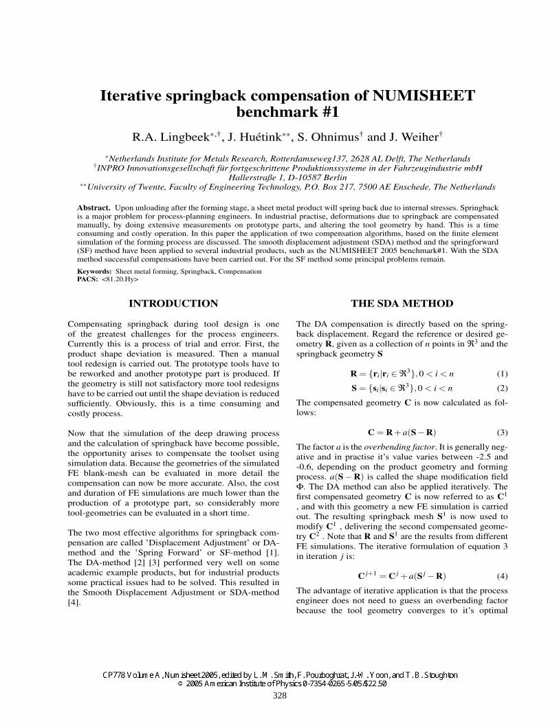
Figure 1. The forming process in PAM-STAMP

bending problem. In reality, springback depends not only

on bending stresses but also on in-plane stresses. This is

important for the compensation. Since the tool geometry

is changed, and not the geometry of the product itself,

the result of the compensation also depends on the be-

havior of the deep drawing process with respect to small

changes in the tool geometry. For 2D bending problems

this response is mainly linear and the results of the (S)DA

algorithm are very good.

A free bending product

The following example process consists of the free

bending of a strip. The process is a simplification of a

real industrial process, and is shown in figure 1. The

process has been modeled in PAM-STAMP 2G 2004.

The forming process was calculated with an explicit

solver, for the springback phase the implicit solver was

used.

The SDA code was implemented in C++. The program

is able to set-up and start PAM-STAMP simulations and

to evaluate the results of the simulation and compensate

the tool meshes, no user interaction is required. During

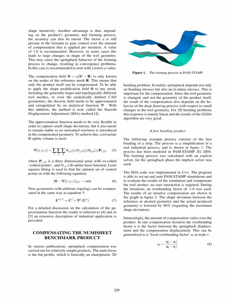
the iterations, an overbending factor of -1.0 was used.

The results of an iterative compensation are shown in

the graph in figure 2. The shape deviation between the

reference or desired geometry and the actual produced

geometry is lowered by 96% (regarding the maximum

shape deviation).

Interestingly, the amount of compensation varies over the

product. In one compensation iteration the overbending

factor a is the factor between the springback displace-

ment and the compensation displacement. This can be

generalized to a ’local overbending factor’ ai at node i:

ai =|ci − ri|

|si − ri|(8)

329

Figure 2. Shape deviation during compensation

Note that for a one-step iteration this value is of course

identical for each node. In the middle of the blank, ai is

about -1.30 (the industry rule-of-thumb), at the sides it is

much lower, around -0.60.

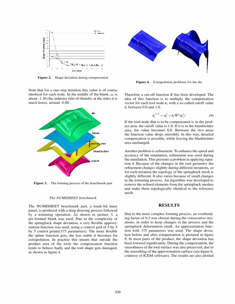
Figure 3. The forming process of the benchmark part

The NUMISHEET benchmark

The NUMISHEET benchmark part, a trunk-lid inner

panel, is produced with a deep drawing process followed

by a trimming operation. As shown in picture 3, a

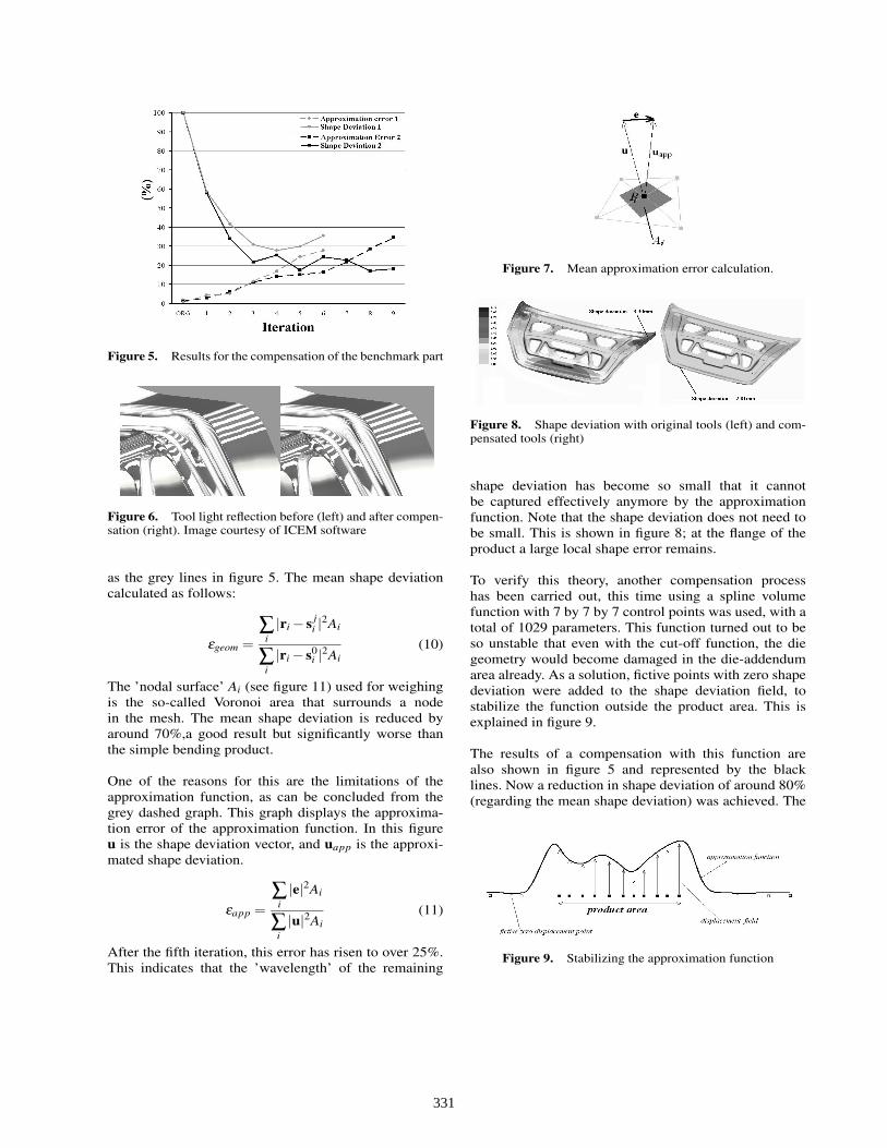
pre-formed blank was used. Due to the complexity of

the springback shape deviation, a very flexible approxi-

mation function was used, using a control grid of 5 by 5

by 5 control points(375 parameters). The more flexible

the spline function gets, the less stable it becomes for

extrapolation. In practise this means that outside the

product area of the tools the compensation function

tends to behave badly and the tool shape gets damaged,

as shown in figure 4.

Figure 4. Extrapolation problems for the die

Therefore a cut-off function K has been developed. The

idea of this function is to multiply the compensation

vector for each tool node ci with a so-called cutoff value

ki between 0.0 and 1.0.

cj+1i = c

ji + kiΨ

j(c ji ) (9)

If the tool-node that is to be compensated is in the prod-

uct area, the cutoff value is 1.0. If it is in the blankholder

area, the value becomes 0.0. Between the two areas

the function value drops smoothly. In this way, detailed

compensation is possible, while leaving the blankholder

area unchanged.

Another problem is refinement. To enhance the speed and

accuracy of the simulation, refinement was used during

the simulation. This presents a problem in applying equa-

tion 4. Because of the changes in the tool geometry the

refinement changes slightly during different iterations, so

for each iteration the topology of the springback mesh is

slightly different. It also varies because of small changes

in the trimming process. An algorithm was developed to

remove the refined elements from the springback meshes

and make them topologically identical to the reference

mesh.

RESULTS

Due to the more complex forming process, an overbend-

ing factor of 0.3 was chosen during the consecutive iter-

ations, in order to keep changes to the process and the

springback deformation small. An approximation func-

tion with 375 parameters was used. The shape devia-

tion before and after compensation is pictured in figure

8. In most parts of the product, the shape deviation has

been lowered significantly. During the compensation, the

smoothness of the tool surface was also preserved, due to

the smoothing of the approximation surface (see figure 6,

courtesy of ICEM software). The results are also plotted

330

Figure 5. Results for the compensation of the benchmark part

Figure 6. Tool light reflection before (left) and after compen-sation (right). Image courtesy of ICEM software

as the grey lines in figure 5. The mean shape deviation

calculated as follows:

εgeom =

∑i

|ri − sji |

2Ai

∑i

|ri − s0i |

2Ai

(10)

The ’nodal surface’ Ai (see figure 11) used for weighing

is the so-called Voronoi area that surrounds a node

in the mesh. The mean shape deviation is reduced by

around 70%,a good result but significantly worse than

the simple bending product.

One of the reasons for this are the limitations of the

approximation function, as can be concluded from the

grey dashed graph. This graph displays the approxima-

tion error of the approximation function. In this figure

u is the shape deviation vector, and uapp is the approxi-

mated shape deviation.

εapp =

∑i

|e|2Ai

∑i

|u|2Ai

(11)

After the fifth iteration, this error has risen to over 25%.

This indicates that the ’wavelength’ of the remaining

Figure 7. Mean approximation error calculation.

Figure 8. Shape deviation with original tools (left) and com-pensated tools (right)

shape deviation has become so small that it cannot

be captured effectively anymore by the approximation

function. Note that the shape deviation does not need to

be small. This is shown in figure 8; at the flange of the

product a large local shape error remains.

To verify this theory, another compensation process

has been carried out, this time using a spline volume

function with 7 by 7 by 7 control points was used, with a

total of 1029 parameters. This function turned out to be

so unstable that even with the cut-off function, the die

geometry would become damaged in the die-addendum

area already. As a solution, fictive points with zero shape

deviation were added to the shape deviation field, to

stabilize the function outside the product area. This is

explained in figure 9.

The results of a compensation with this function are

also shown in figure 5 and represented by the black

lines. Now a reduction in shape deviation of around 80%

(regarding the mean shape deviation) was achieved. The

Figure 9. Stabilizing the approximation function

331

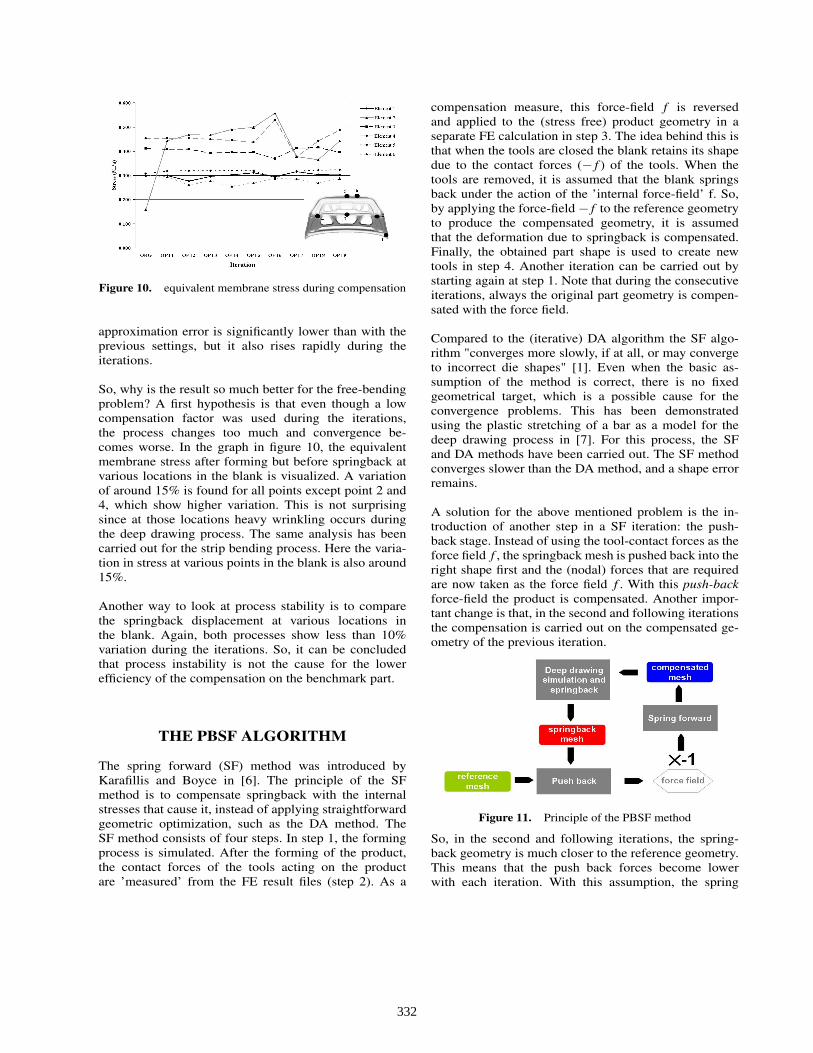
Figure 10. equivalent membrane stress during compensation

approximation error is significantly lower than with the

previous settings, but it also rises rapidly during the

iterations.

So, why is the result so much better for the free-bending

problem? A first hypothesis is that even though a low

compensation factor was used during the iterations,

the process changes too much and convergence be-

comes worse. In the graph in figure 10, the equivalent

membrane stress after forming but before springback at

various locations in the blank is visualized. A variation

of around 15% is found for all points except point 2 and

4, which show higher variation. This is not surprising

since at those locations heavy wrinkling occurs during

the deep drawing process. The same analysis has been

carried out for the strip bending process. Here the varia-

tion in stress at various points in the blank is also around

15%.

Another way to look at process stability is to compare

the springback displacement at various locations in

the blank. Again, both processes show less than 10%

variation during the iterations. So, it can be concluded

that process instability is not the cause for the lower

efficiency of the compensation on the benchmark part.

THE PBSF ALGORITHM

The spring forward (SF) method was introduced by

Karafillis and Boyce in [6]. The principle of the SF

method is to compensate springback with the internal

stresses that cause it, instead of applying straightforward

geometric optimization, such as the DA method. The

SF method consists of four steps. In step 1, the forming

process is simulated. After the forming of the product,

the contact forces of the tools acting on the product

are ’measured’ from the FE result files (step 2). As a

compensation measure, this force-field f is reversed

and applied to the (stress free) product geometry in a

separate FE calculation in step 3. The idea behind this is

that when the tools are closed the blank retains its shape

due to the contact forces (− f ) of the tools. When the

tools are removed, it is assumed that the blank springs

back under the action of the ’internal force-field’ f. So,

by applying the force-field − f to the reference geometry

to produce the compensated geometry, it is assumed

that the deformation due to springback is compensated.

Finally, the obtained part shape is used to create new

tools in step 4. Another iteration can be carried out by

starting again at step 1. Note that during the consecutive

iterations, always the original part geometry is compen-

sated with the force field.

Compared to the (iterative) DA algorithm the SF algo-

rithm "converges more slowly, if at all, or may converge

to incorrect die shapes" [1]. Even when the basic as-

sumption of the method is correct, there is no fixed

geometrical target, which is a possible cause for the

convergence problems. This has been demonstrated

using the plastic stretching of a bar as a model for the

deep drawing process in [7]. For this process, the SF

and DA methods have been carried out. The SF method

converges slower than the DA method, and a shape error

remains.

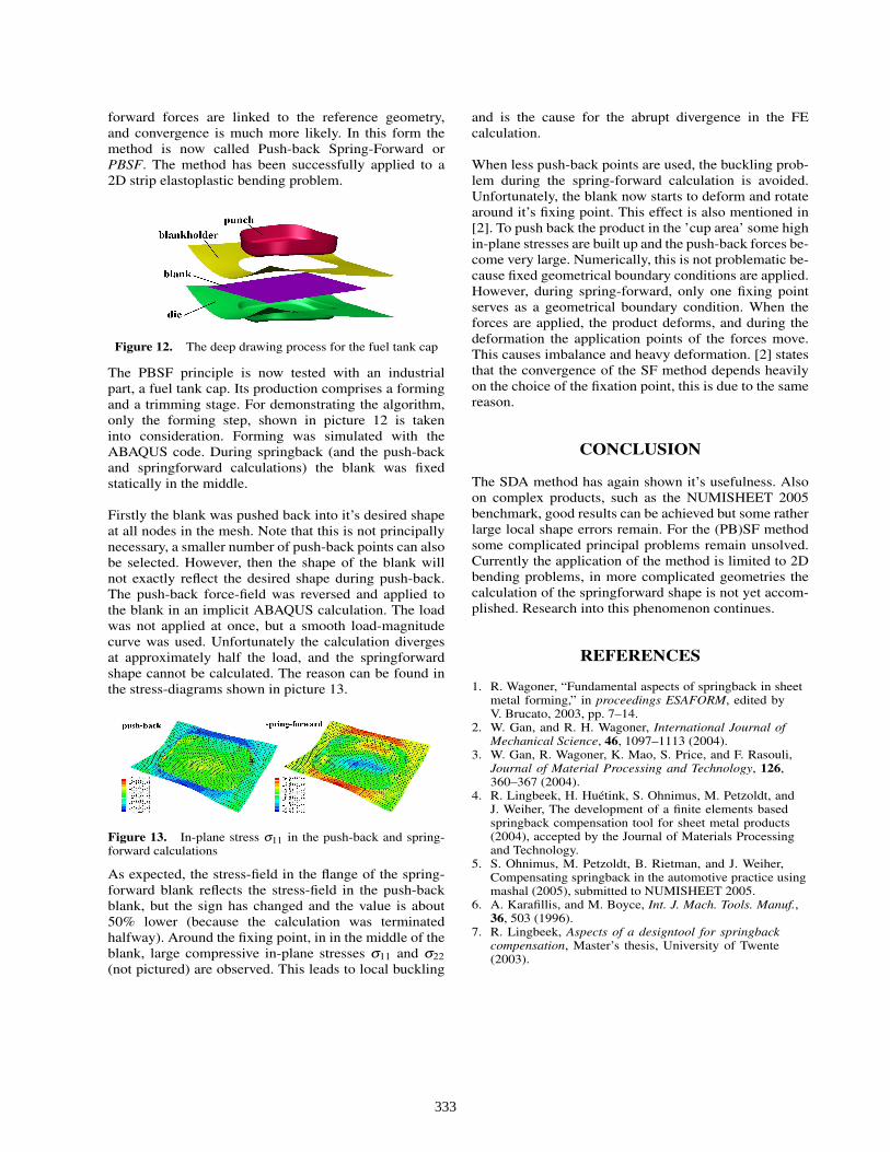
A solution for the above mentioned problem is the in-

troduction of another step in a SF iteration: the push-

back stage. Instead of using the tool-contact forces as the

force field f , the springback mesh is pushed back into the

right shape first and the (nodal) forces that are required

are now taken as the force field f . With this push-back

force-field the product is compensated. Another impor-

tant change is that, in the second and following iterations

the compensation is carried out on the compensated ge-

ometry of the previous iteration.

Figure 11. Principle of the PBSF method

So, in the second and following iterations, the spring-

back geometry is much closer to the reference geometry.

This means that the push back forces become lower

with each iteration. With this assumption, the spring

332

forward forces are linked to the reference geometry,

and convergence is much more likely. In this form the

method is now called Push-back Spring-Forward or

PBSF. The method has been successfully applied to a

2D strip elastoplastic bending problem.

Figure 12. The deep drawing process for the fuel tank cap

The PBSF principle is now tested with an industrial

part, a fuel tank cap. Its production comprises a forming

and a trimming stage. For demonstrating the algorithm,

only the forming step, shown in picture 12 is taken

into consideration. Forming was simulated with the

ABAQUS code. During springback (and the push-back

and springforward calculations) the blank was fixed

statically in the middle.

Firstly the blank was pushed back into it’s desired shape

at all nodes in the mesh. Note that this is not principally

necessary, a smaller number of push-back points can also

be selected. However, then the shape of the blank will

not exactly reflect the desired shape during push-back.

The push-back force-field was reversed and applied to

the blank in an implicit ABAQUS calculation. The load

was not applied at once, but a smooth load-magnitude

curve was used. Unfortunately the calculation diverges

at approximately half the load, and the springforward

shape cannot be calculated. The reason can be found in

the stress-diagrams shown in picture 13.

Figure 13. In-plane stress σ11 in the push-back and spring-forward calculations

As expected, the stress-field in the flange of the spring-

forward blank reflects the stress-field in the push-back

blank, but the sign has changed and the value is about

50% lower (because the calculation was terminated

halfway). Around the fixing point, in in the middle of the

blank, large compressive in-plane stresses σ11 and σ22

(not pictured) are observed. This leads to local buckling

and is the cause for the abrupt divergence in the FE

calculation.

When less push-back points are used, the buckling prob-

lem during the spring-forward calculation is avoided.

Unfortunately, the blank now starts to deform and rotate

around it’s fixing point. This effect is also mentioned in

[2]. To push back the product in the ’cup area’ some high

in-plane stresses are built up and the push-back forces be-

come very large. Numerically, this is not problematic be-

cause fixed geometrical boundary conditions are applied.

However, during spring-forward, only one fixing point

serves as a geometrical boundary condition. When the

forces are applied, the product deforms, and during the

deformation the application points of the forces move.

This causes imbalance and heavy deformation. [2] states

that the convergence of the SF method depends heavily

on the choice of the fixation point, this is due to the same

reason.

CONCLUSION

The SDA method has again shown it’s usefulness. Also

on complex products, such as the NUMISHEET 2005

benchmark, good results can be achieved but some rather

large local shape errors remain. For the (PB)SF method

some complicated principal problems remain unsolved.

Currently the application of the method is limited to 2D

bending problems, in more complicated geometries the

calculation of the springforward shape is not yet accom-

plished. Research into this phenomenon continues.

REFERENCES

1. R. Wagoner, “Fundamental aspects of springback in sheetmetal forming,” in proceedings ESAFORM, edited byV. Brucato, 2003, pp. 7–14.

2. W. Gan, and R. H. Wagoner, International Journal ofMechanical Science, 46, 1097–1113 (2004).

3. W. Gan, R. Wagoner, K. Mao, S. Price, and F. Rasouli,Journal of Material Processing and Technology, 126,360–367 (2004).

4. R. Lingbeek, H. Huétink, S. Ohnimus, M. Petzoldt, andJ. Weiher, The development of a finite elements basedspringback compensation tool for sheet metal products(2004), accepted by the Journal of Materials Processingand Technology.

5. S. Ohnimus, M. Petzoldt, B. Rietman, and J. Weiher,Compensating springback in the automotive practice usingmashal (2005), submitted to NUMISHEET 2005.

6. A. Karafillis, and M. Boyce, Int. J. Mach. Tools. Manuf.,36, 503 (1996).

7. R. Lingbeek, Aspects of a designtool for springbackcompensation, Master’s thesis, University of Twente(2003).

333