Investigation of Wall Pressure Fluctuations Induced by Turbulent Boundary Layer Flow with Pressure Gradients Bei der Fakultät für Maschinenbau der Technischen Universität Carolo-Wilhelmina zu Braunschweig zur Erlangung der Würde eines Doktor-Ingenieurs (Dr.-Ing.) genehmigte Dissertation von: Nan Hu geboren in (Geburtsort): Beijing, China eingereicht am: 04.01.2018 mündliche Prüfung am: 29.05.2018 Vorsitz: Jun.-Prof. Dr. R. A. D. Akkermans Gutachter: Prof. Dr.-Ing. J. W. Delfs Prof. Dr.-Ing. W. Schröder 2018
Transcript
Investigation of Wall Pressure Fluctuations Inducedby Turbulent Boundary Layer Flow with Pressure
Gradients
Bei der Fakultät für Maschinenbau
der Technischen Universität Carolo-Wilhelmina zu Braunschweig
zur Erlangung der Würde
eines Doktor-Ingenieurs (Dr.-Ing.)
genehmigte Dissertation
von: Nan Hugeboren in (Geburtsort): Beijing, China
Vorsitz: Jun.-Prof. Dr. R. A. D. AkkermansGutachter: Prof. Dr.-Ing. J. W. Delfs
Prof. Dr.-Ing. W. Schröder
2018
Abstract
Wall pressure fluctuations induced by turbulent boundary layer flow is one major sourceof cabin noise. Not only the pressure fluctuation magnitude but also the spatial andtemporal properties of the fluctuations are relevant for the resulting surface vibration andthe noise radiated into the cabin. The one- and two-point properties of the wall pressurefluctuations are studied experimentally and numerically in thesis thesis.The wall pressure fluctuations beneath a turbulent boundary layer with zero and non-
zero pressure gradients were measured at a flat plate configuration in the AeroacousticWind Tunnel Braunschweig. The fluctuating pressure was measured by an L-shaped arrayof subminiature pressure transducers. The mean flow velocity profiles and the Reynoldsstresses within the turbulent boundary layer were obtained using single and crossed hot-wire anemometers, respectively. Adverse and favorable pressure gradients were realizedby installing a turnable NACA 0012 airfoil above the plate. The one-point spectrum, thecorrelation in the streamwise and spanwise directions and the convection velocity for thewall pressure field are analyzed. The effect of the pressure gradients on the wall pressurefluctuations and the corresponding relevant boundary layer parameters are discussed.Based on the measured data and a dataset of four other experiments at three other test
facilities, an empirical model of wall pressure spectra for adverse pressure gradient bound-ary layers is proposed. Goody’s model, which is the most used wall pressure spectrummodel for zero pressure gradient boundary layers, is served as the basis for the developmentof the new model. Predictions of the new model and comparisons with other publishedwall pressure spectral models for adverse pressure gradient boundary layers are made forthe selected dataset. The new model shows good prediction accuracy for the selecteddataset and a significant improvement compared to the other published models.Furthermore, pressure fluctuations within turbulent boundary layers on a flat plate
configuration are simulated using synthetic isotropic and anisotropic turbulence generatedby the Fast Random Particle-Mesh Method. The averaged turbulence statistics neededfor the stochastic realization is provided by a Reynolds averaged Navier-Stokes simulation.Anisotropy of integral lengths scales and Reynolds stress tensors are implemented for therealization of anisotropic turbulence. To determine the fluctuating pressure, a Poisson’sequation is solved with unsteady right-hand side source terms derived from the syntheticturbulence realization. The Poisson’s equation is solved via fast Fourier transform usingHockney’s method. Due to its efficiency, the applied procedure enables us to study, for highReynolds number flow, the effect of variations of the modelled turbulence characteristicson the resulting wall pressure spectrum. The contributions to wall pressure fluctuationsfrom the mean-shear turbulence interaction term and the turbulence-turbulence interactionterm are studied separately. The results show that both contributions have the same orderof magnitude. Simulated one-point spectra and two-point correlations of wall pressurefluctuations are analyzed in detail. Convective features of the fluctuating pressure field arewell determined. Good agreement for the characteristics of the wall pressure fluctuationsis found between the numerical results and databases from the present measured data andother investigators.
Zusammenfassung
Die durch turbulente Grenzschichtströmung induzierten Wanddruckschwankungen sindeine Hauptquelle von Kabinenlärm. Für die resultierende Oberflächenschwingung und dasin die Kabine abgestrahlte Geräusch sind nicht nur die Druckschwankungsstärke, son-dern auch die räumlichen und zeitlichen Eigenschaften der Schwankungen relevant. DieEin- und Zweipunkt-Eigenschaften der Wanddruckschwankungen werden in dieser Arbeitexperimentell und numerisch untersucht.Die Wanddruckschwankungen in einer turbulenten Grenzschicht mit Null- und Nicht-
Null-Druckgradienten wurden im Aeroakustischen Windkanal Braunschweig an einer fla-chen Plattenkonfiguration gemessen. Der schwankende Druck wurde mit einer L-förmigenAnordnung von Subminiatur-Druckwandlern gemessen. Die mittleren Geschwindigkeits-profile und die Reynoldsspannungen innerhalb der turbulenten Grenzschicht wurden unterVerwendung von einzelnen bzw. gekreuzten Hitzdrahtanemometern ermittelt. Positiveund negative Druckgradienten wurden durch die Installation eines drehbaren NACA 0012Profils über der Platte generiert. Das Einpunkt-Spektrum, die Korrelation in der Strö-mungsrichtung und der Querrichtung und die Konvektionsgeschwindigkeit für den Wand-druck werden analysiert. Die Auswirkung der Druckgradienten auf die Wanddruckschwan-kungen und die entsprechenden relevanten Grenzschichtparameter werden diskutiert.Basierend auf den gemessenen Daten und einem Datensatz von vier weiteren Experi-
menten an drei weiteren Versuchsanlagen wird ein empirisches Modell vonWanddruckspek-tren für positive Druckgradientengrenzschichten vorgeschlagen. Das Modell von Goody,welches das am meisten verwendete Wanddruckspektrum für Grenzschichten mit Null-Druckgradienten ist, dient als Grundlage für die Entwicklung des neuen Modells. Vorher-sagen des neuen Modells und Vergleiche mit anderen veröffentlichten Wanddruckspek-tralmodellen für Grenzschichten mit positiven Druckgradienten werden für den ausgewähl-ten Datensatz durchgeführt. Das neue Modell zeigt eine gute Vorhersagegenauigkeit fürden ausgewählten Datensatz und eine signifikante Verbesserung im Vergleich zu den an-deren veröffentlichten Modellen.Außerdem werden Druckschwankungen innerhalb turbulenter Grenzschichten auf einer
flachen Plattenkonfiguration mit den synthetischen isotropen und anisotropischen Tur-bulenzen simuliert, wobei diese durch die Fast Random Particle-Mesh-Methode erzeugtwerden. Die gemittelte Turbulenzstatistik, die für die stochastische Modellierung benötigtwird, wird durch eine Reynolds-gemittelte Navier-Stokes Simulation bereitgestellt. Aniso-tropie von Längenskalen und Reynolds-Spannungstensoren werden für die Modellierungvon anisotropen Turbulenzen implementiert. Um den schwankenden Druck zu bestim-men, wird eine Poisson-Gleichung mit instationären rechtsseitigen Quellterme gelöst, deraus der synthetischen Turbulenzerzeugung abgeleitet wird. Die Poisson-Gleichung wirdmittels schneller Fourier-Transformation unter Verwendung der Hockney-Methode gelöst.Aufgrund seiner Effizienz ermöglicht es das angewandte Verfahren, den Einfluss von Varia-tionen der modellierten Turbulenzeigenschaften auf das resultierende Wanddruckspek-trum für eine hohe Reynoldszahl-Strömung zu untersuchen. Die Beiträge zu Wanddruck-schwankungen aus dem Mittelscherung-Turbulenz-Wechselwirkungsterm und dem Turbu-lenz-Turbulenz-Wechselwirkungsterm werden getrennt untersucht. Die Ergebnisse zeigen,dass beide Beiträge die gleiche Größenordnung haben. Simulierte Einpunkt-Spektren
und Zweipunkt-Korrelationen von Wanddruckschwankungen werden im Detail analysiert.Konvektive Eigenschaften des fluktuierenden Druckfeldes werden gut bestimmt. Einegute Übereinstimmung hinsichtlich der Eigenschaften der Wanddruckschwankungen findetsich zwischen den numerischen Ergebnissen, den vorliegenden Messdaten und externenForschungsergebnissen.
vi
Acknowledgement
The results of this work have been achieved within the DLR project Comfort and EfficiencyEnhancing Technologies (CENT). The completion of the Ph.D study is a learning process,not only in the scientific field, but also on a personal level. All happiness and frustrationduring the study are important life experience for me. Without the help of my supervisor,my colleagues and my family, I would have never accomplished the study. Therefore, Iwould like to thank all of you for your support and encouragement.First of all, I would like to thank my supervisor Prof. Dr.-Ing. Jan Delfs for the valuable
discussions and advices throughout the study that helped to improve the quality of thecurrent work. My special thanks go to the reviewer Prof. Dr.-Ing.Wolfgang Schröder andthe chairman Jun.-Prof. Dr. Rinie Akkermans. I would like also to thank my indispensablementors Dr.-Ing.Roland Ewert and Dr.-Ing.Michaela Herr for sharing their knowledgeand experience in numerical and experimental aeroacoustics and also in scientific writings.Furthermore, many thanks are due to my office mate M. Sc.Karl-Stephane Rossignol forthe pleasant professional and personal conversations. I would like also to thank my col-leagues Dipl.-Ing.Nils Reiche and Dr.-Ing. Christina Appel for their help of the numericalstudies and Dipl.-Ing.Michael Pott-Pollenske, Dipl.-Ing.Heino Buchholz, Danica Knoblichand Jan Täger for their support and assurance for the performance of the experiments.Last, but not the least, I am especially grateful to my parents and my wife for their
encouragement during my Ph.D study and also my life’s tough times.
βδ, β∆ Clauser’s equilibrium parameter related to other boundary layer parameters,(δ,∆)/Q· dp/dx
βδ∗ , βθ boundary layer thickness and displacement thickness based Clauser’s equilib-rium parameter, (δ∗, θ)/τw · dp/dx
∆ boundary layer defect thickness, δ∗√
2/Cf , or Laplace operator ∇·∇
δ boundary layer thickness or Dirac delta function
δ∗ boundary layer displacement thickness
∆δ/δ∗ boundary layer related parameter, δ/δ∗
Γ coherence
κ Von Kármán constant
Ui spatial white noise
∇ gradient of
∇· divergence of
∇× curl of
ν kinematic viscosity
ω angular frequency
Φ spectrum
φm moving axis spectrum
Πθ Cole’s wake parameter related to the boundary layer momentum thickness,0.8 · (βθ + 0.5)3/4
Πδ∗ Cole’s wake parameter, 0.8 · (βδ∗ + 0.5)3/4
ρ density
ρ′ density fluctuations
ρ0 mean ambient density
xi
Contents
τw wall shear stress
θ boundary layer momentum thickness or phase difference
a0 speed of sound
Cf skin friction coefficient, τw/Q
Cp pressure coefficient
f frequency
G Gaussian filter kernel
H boundary layer shape parameter, δ/δ∗
k wavenumber
l length scale
p pressure
p′ pressure fluctuations
Q dynamic pressure, 0.5ρU20 , or the source term of the Poisson’s equation
R correlation
r distance
RT time scale ratio, (δ/Ue)/(ν/u2τ )
Reτ wall shear stress based Reynolds number, uτδ/ν
Reθ boundary layer momentum thickness based Reynolds number, U0θ/ν
Reδ, Re∆ Reynolds number related to other boundary layer parameters, (δ,∆)Ue/ν
t, τ time
u velocity
u′ velocity fluctuations
u+ dimensionless velocity, u/uτ
uτ friction velocity,√τw/ρ
uc, Uc convection velocity
Ue, U0 boundary layer edge velocity and local free-stream velocity
x, y, z spatial coordinates
y+ dimensionless wall-normal coordinate, yuτ/ν
xii
Contents
Abbreviations
1,2,3-D one, two, three-dimensional
AOA angle of attack
APG adverse pressure gradient
AWB Aeroacoustic Wind Tunnel Braunschweig
CFAS Catlett et al.
CFD computational fluid dynamics
CFL Courant-Friedrichs-Lewy
DNS direct numerical simulation
FPG favorable pressure gradient
FRPM Fast Random Particle-Mesh Method
KBLWK Kamruzzaman et al.
LES large eddy simulation
MS mean-shear term
NACA National Advisory Committee for Aeronautics
PSD power spectral density
RANS Reynolds-averaged Navier-Stokes
RRM Rozenberg et al.
TT turbulence-turbulence term
XFOIL Subsonic Airfoil Development System
ZPG zero pressure gradient
xiii
1 Introduction
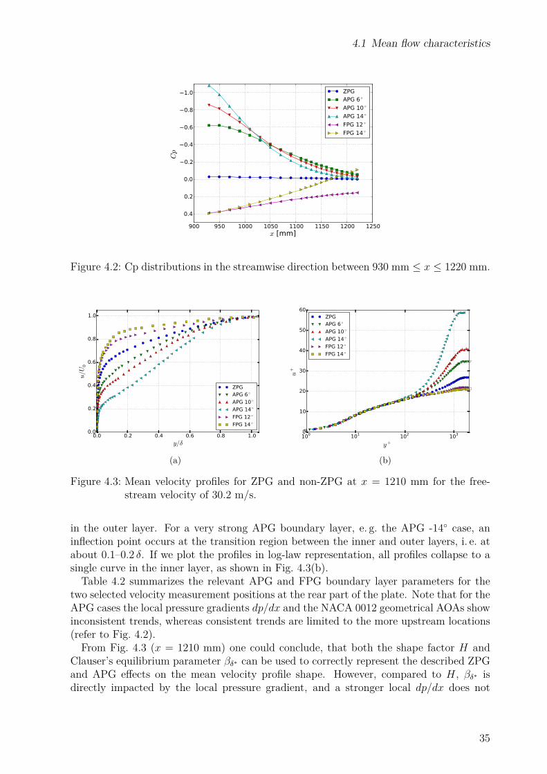
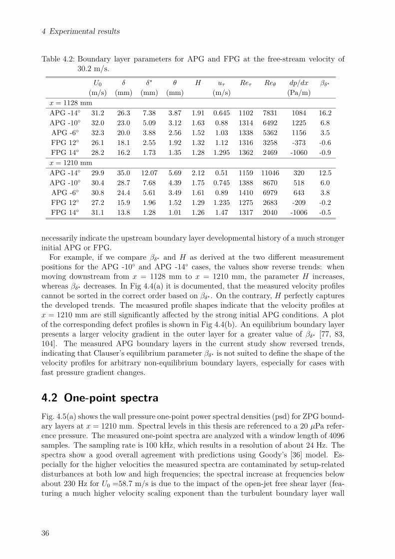
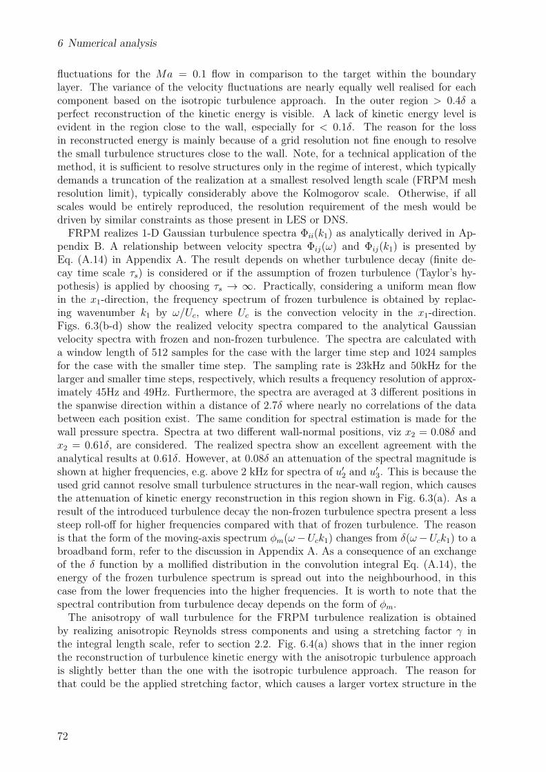
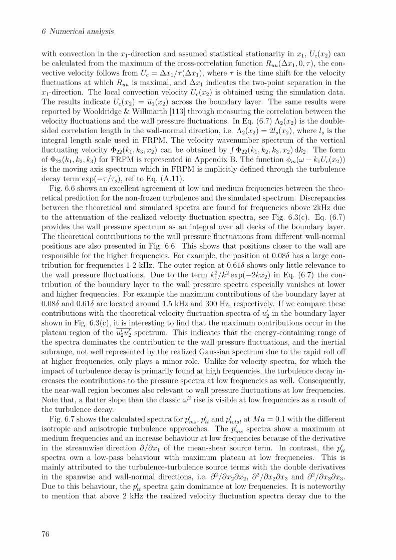
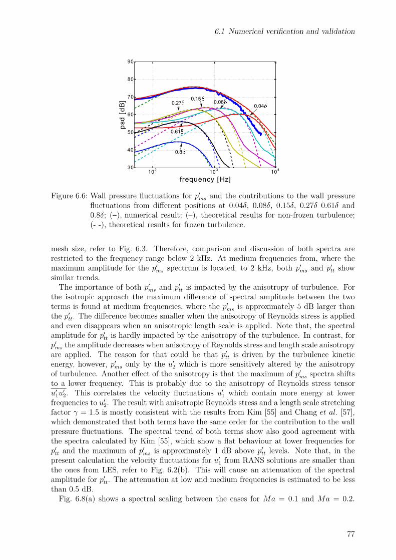
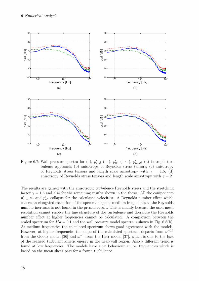
1.1 Motivation and backgroundAeroacoustics is a relatively new branch of aerodynamics and it has gained more impor-tance due to the increasing demand for noise reduction and comfort in the field of aircraft,vehicles and wind turbines. Wall pressure fluctuations beneath a turbulent boundary layerare a fundamental topic in flow-induced noise. One major concern is the noise transmissionthrough the elastic structure below the surface due to the fluctuating pressure excitationon the surface. The pressure fluctuations caused by the fluctuating velocities, exert anunsteady loading on the surface and consequently the induced surface vibration radiatesnoise, which makes the wall pressure fluctuations an important noise source for the cabin,especially for the aircraft cabin. This phenomenon has become more important with the re-duction of jet and fan noise during the development of the jet engine over the past decades.Nowadays, the noise caused by wall pressure fluctuations beneath a turbulent boundarylayer becomes a major source for aircraft cabin noise in cruise flight [1, 2]. Since cabinnoise belongs to one of the decisive conditions for the airline passenger comfort, predictionand reduction of turbulent boundary layer induced wall pressure fluctuations become moreinvolved in the aircraft design process. To achieve a low-noise design, a deep understandingof this phenomenon and applicable design tools are required. The knowledge on wall pres-sure fluctuations gained over the past decades is mostly restricted to non-ac-/deceleratedtime averaged flows, i.e. mean flows characterized by zero pressure gradient (ZPG). How-ever, in reality, a non-ZPG boundary layer occurs in most cases. Therefore, there is a highdemand for investigations of the effect of pressure gradients on wall pressure fluctuations.Furthermore, numerical tools based on resolving (fully or partially) wall turbulence arehardly applicable for practical design applications (characterized by Reynolds numbers onthe order of 100M) due to the extremely high computational costs. Therefore, an efficientnumerical method, which can represent the most important features of the wall pressurefield relevant to cabin noise excitation, is of particular interest.The phenomenon of the turbulent boundary layer induced wall pressure fluctuations was
pioneered by Kraichnan [3] and Willmarth [4] in the 1950s. The theoretical work fromKraichnan identified that the pressure fluctuations within an incompressible boundarylayer is governed by a Poisson’s equation and the fluctuating pressure is caused by a linearmean-shear turbulence interaction term and a non-linear turbulence-turbulence interactionterm. Willmarth measured some properties for the one-point statistics of the wall pressurefluctuations at different Reynolds numbers and Mach numbers. Since then, extensivetheoretical and experimental work has been done to investigate the characteristics of thewall pressure field. Focus of the investigations has not only been on the one-point statistics,but also on the two-point statistics because of the importance of the space-time featuresto the surface structural response.A comprehensive understanding of the wall pressure field was firstly gained by the
experimental results from Willmarth & Wooldridge [5]. They measured both one- andtwo-point statistics of the wall pressure fluctuations beneath a thick ZPG boundary layer
1
1 Introduction
in a subsonic wind tunnel and analyzed the properties of the pressure field extensively.Such measurements concentrated on investigations of the wall pressure power spectra,space-time correlations, cross-spectra while investigations on the convective features wereconducted by Bull [6], Blake [7], Farabee & Casarella [8] and Leclercq & Bohineust [9].In the meantime, there has been growing interest in direct measurements of the wall
pressure wavenumber-frequency spectra. The wavenumber-frequency spectra are just an-other interpretation of the space-time properties, and can provide a more intuitive meansof analysis of the structure-vibrational response to the wall pressure excitation. In theearly stage, Blake & Chase [10] and Farabee & Geib [11] used spatial-filtering to measurethe wavenumber-frequency spectra by a couple of microphones arranged in the streamwisedirection. With the development of measuring devices and processing techniques, Abra-ham & Keith [12], Arguillat et al. [13], Ehrenfried & Koop [14] and Gabriel et al. [15]measured the wavenumber-frequency spectra by using array technology. In their measure-ments the convective ridge and the acoustic part can be well identified. However, due tothe applied array size and the background noise of the test facilities, the obtained spectrain the low-wavenumber or low-frequency range were still not conclusive.Another general difficulty of experimentally acquiring the wall pressure fluctuations is
to precisely measure the spectra in the high-frequency or high-wavenumber range. Dueto the averaging effect on waves by a sensor surface, an attenuation of the wall pressuremagnitude will be measured at a high wavenumber range with respect to the sensor size.This effect was first studied by Corcos [16], who established the relationship betweenthe sensor size and the caused spectral attenuation beneath a turbulent boundary layer.Later, experimental and theoretical studies on this effect were given by Gilchrist [17],White [18], Chase [19] and Bull [20]. To circumvent this problem, the ’effective’ sensorsurface needs to be reduced. Therefore, sensors with a pinhole setup were often applied.Even with the pinhole configuration, the measurable frequency range is limited by theHelmholtz resonance frequency. To be able to measure at higher frequencies, a higherresonance frequency is essential, i.e. a smaller sensor is required. In recent experimentalstudies, sub-miniature pressure sensors were more and more applied. By now, the smallestavailable sensor for the pressure measurement has a diameter of 1.6 mm. Note, even withthe smallest size, a flush-mounted sensor is still too ’large’ for measuring the wall pressurein the high frequency range.Besides wind tunnel measurements, measurements of the wall pressure fluctuations have
been also carried out directly on airplanes. The measurement station was placed at thewing in the early flight tests [21, 22]. In the later tests [23, 24, 25, 26], the focus laid on theturbulent boundary layer induced cabin noise and therefore pressure fluctuations on thefuselage were measured. A highlight of the most recent flight test was the measurementof wavenumber-frequency spectra using array technology [27].There has always been an interest in the prediction of the magnitude and the space-
time features of the wall pressure field. Theoretical works of prediction of the mean squarepressure were given by Kraichnan [3], Lilley [28], Meecham & Tavis [29] and Chase [30].Later, Farabee & Casarella [8] and Viazzo et al. [31] estimated the magnitude by inte-grating the one-point spectra in the frequency domain with consideration of the Reynoldsnumber effect. One-point spectral models were proposed by Robertson [32], Chase [30],Efimtsov [33], Howe [34], Smol’yakov [35], Goody [36] and Herr [37]. Most of the modelswere derived for prediction of low-speed ZPG boundary layers. Robertson’s and Efimtsov’smodels were derived based on in-flight measurements.
2
1.2 State of the art
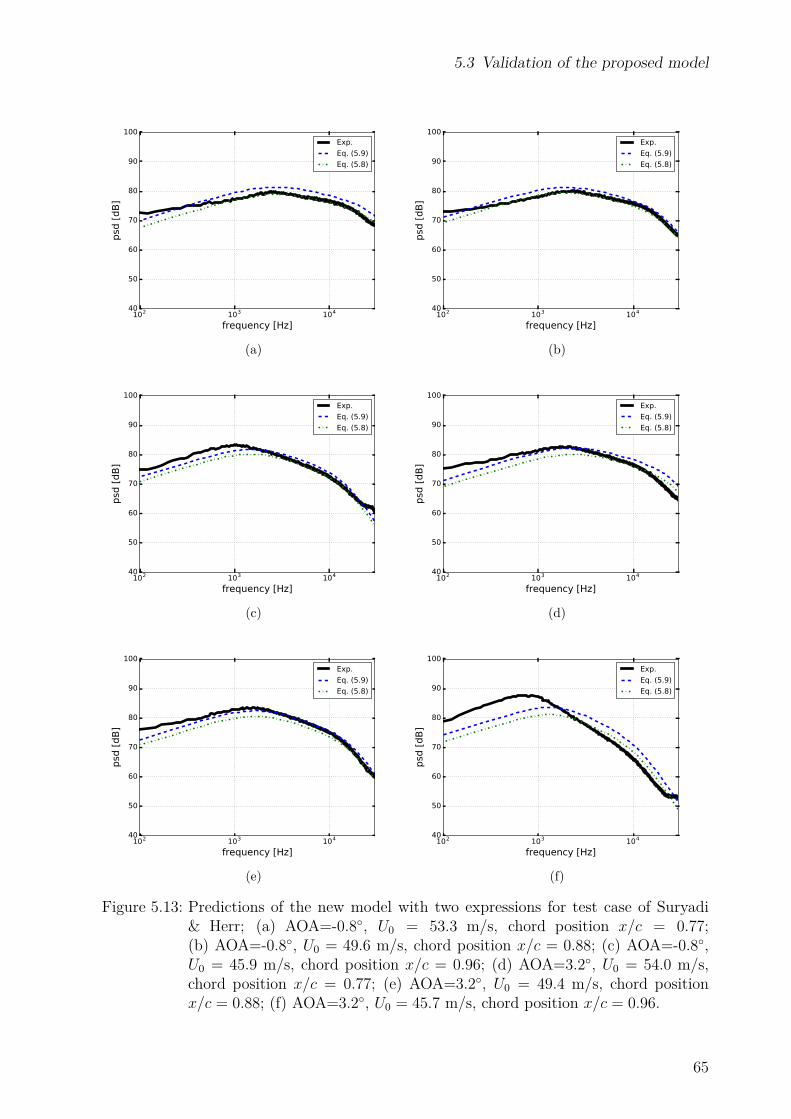
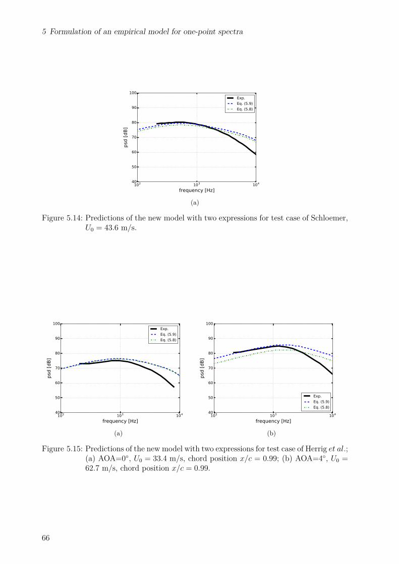
Schloemer [38] was the first to measure wall pressure fluctuations under non-ZPGs.Later, Burton [39], Blake [40] and Simpson [41] further studied this problem under differ-ent flow conditions. Recent measurements were given by Herrig [42], Catlett et al. [43],Salze et al. [44] and Suryadi & Herr [45]. Rozenberg et al. [46], Kamruzzaman et al. [47]and Catlett et al. [48] proposed one-point spectral models for wall pressure fluctuationsunder adverse pressure gradient (APG) boundary layers.Furthermore, the one-point spectra can be also calculated using integration methods
developed by Panton & Linebarger [49] and Blake [50]. The method requires some pa-rameters of the boundary layers, such as mean velocity profiles, Reynolds stresses andturbulent length scales.A model for the description of the space-time correlations was first proposed by Corcos
[51]. Based on experimental results, Corcos found the existence of similarities of thewall pressure cross-spectra for both streamwise and spanwise directions and proposeda cross-spectral model with consideration of the correlation decay and the convectivefeatures of the wall pressure field. Chase [30] did a comprehensive theoretical study ofcharacteristics of wall pressure fluctuations and proposed a model in the wavenumber-frequency domain. The compressibility was not taken into account in the proposed models,which was discussed in the works of Ffowcs Williams [52] and Chase [53].With the booming development of computer technology, the numerical simulation has
become a powerful resource for investigating the fluctuating pressure field. Direct numer-ical simulation (DNS) and large eddy simulation (LES) for the wall pressure fluctuationshave been published by Spalart [54], Kim [55], Choi & Moin [56], Chang et al. [57], Vi-azzo et al. [31] and Gloerfelt & Berland [58]. The properties of wall pressure fluctuations,which are not possible or hard to measure experimentally, can be studied through nu-merical work and new insight can be gained. Although the turbulent boundary layercan be solved by DNS and LES, due to the extremely expensive computation resourcesthe application is generally restricted to generic studies for low and medium Reynoldsnumbers.For a practical application, the requirements on computational resources need to be
further reduced. Stochastic models for calculating the wall pressure fluctuations wereapplied in the works of Siefert et al. [59] and Alaoui et al. [60]. Siefert et al. synthesizeddirectly the wall pressure fluctuation field concentrating on realization of the relevantfeatures for excitation on a surface structure. The method used by Alaoui et al. was basedon the coherent vortex structure of a hairpin model.A summary of the so far acquired knowledge on wall pressure fluctuations beneath
a turbulent boundary layer was given by Willmarth [61] and Bull [62]. A comprehensiveoverview on the subject of wall pressure fluctuations, including also the structural responseand the induced sound radiation was given in the monograph of Blake [50].
1.2 State of the artA brief summary of the background knowledge on wall pressure fluctuations beneath aturbulent boundary layer is given in the previous section. The investigations were mainlyconcentrated on studies of the sources, the one- and two-point statistics of the pressurefield. Some relevant knowledge acquired so far will be addressed in this section.Kraichnan [3] reformulated the Navier-Stokes equations, and derived a Poisson’s equa-
3
1 Introduction
tion, which governs the pressure fluctuations within an incompressible turbulent bound-ary layer. The source terms consisting of a mean-shear turbulence interaction term∂2uiu
′j/∂xi∂xj and a turbulence-turbulence interaction term ∂2(u′iu′j−u′iu′j)/∂xi∂xj, where
ui is the ith cartesian mean flow velocity component and u′i represents the respective ve-locity fluctuation component, are placed on the right-hand side of the Poisson’s equation.The former and the latter denote the interaction between the mean flow and the turbulentfluctuations and the interaction between the turbulent fluctuations themselves, respec-tively. The mean-shear term is a linear term and also called the ’rapid’ term, because ofthe rapid response to a change of the mean flow condition. The turbulence-turbulenceterm is a non-linear term and also called the ’slow’ term due to the slow reaction of thechange through the turbulence-turbulence interactions [55].Determination of the relative influence of each source term on the wall pressure fluctu-
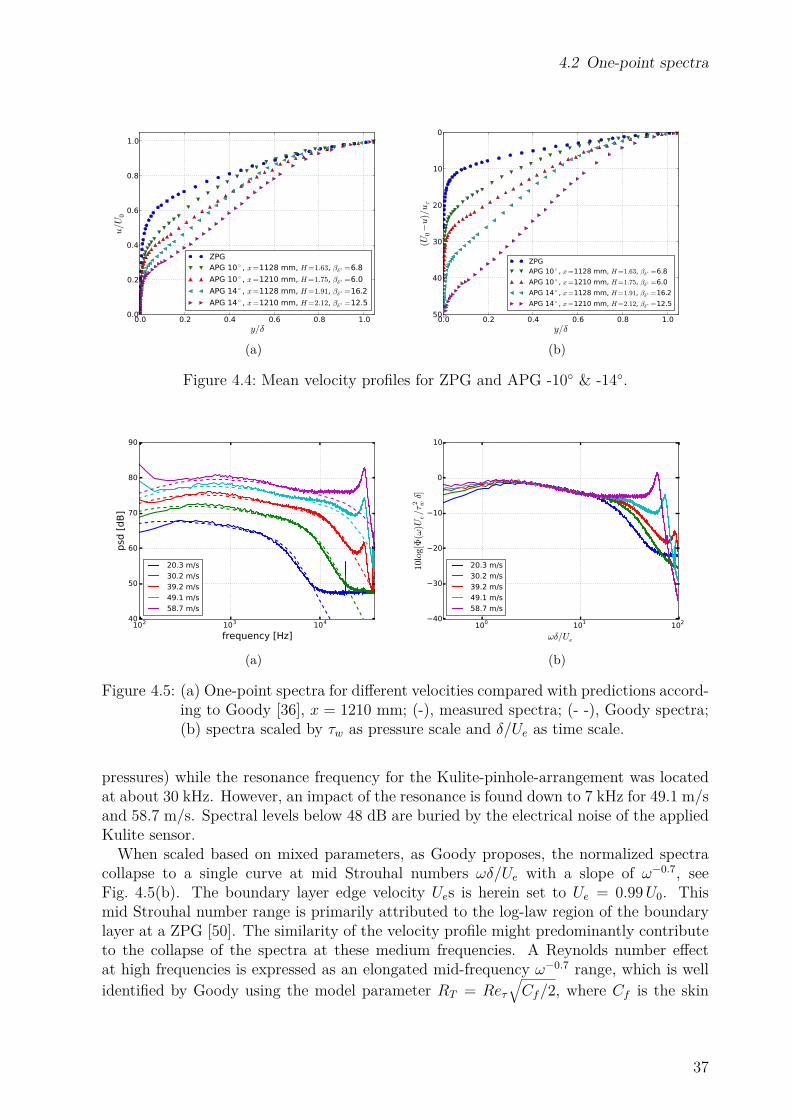
ations has always been of particular interest, because in general only the dominant sourceterm needs to be considered. However, a distinction of the contributions and the impor-tance of both source terms is difficult to be achieved experimentally; most works on thistopic were conducted theoretically. Kraichnan [3], Hodgson [22] and Meecham & Tavis [29]calculated the contribution from the turbulence-turbulence term based on an assumptionof isotropic turbulence with a Gaussian correlation and concluded that the mean-shearterm is the dominant source term for the wall pressure fluctuations. Corcos [51] estimatedthe importance between both sources by comparing the calculated auto-correlation of themean-shear term and the measured auto-correlation and found the magnitude of wall pres-sure fluctuations from the mean-shear term to be somewhat more than 3 dB larger thanfrom the turbulence-turbulence term. Chase [30] did a comprehensive theoretical work onmodeling the wall pressure spectra contributed from both sources and obtained a similarresult as concluded by Corcos. Peltier & Hambric [63] calculated the one-point spectrabased on the turbulence statistics provided by Reynolds-averaged Navier-Stokes equations(RANS) calculations. The result showed that the dominance of the mean-shear term ismore pronounced for a favorable pressure gradient (FPG) boundary layer. An experimen-tal work was conducted by Johansson [64], who used a conditional averaging technique tomeasure the relationship between the fluctuating flow field and the wall pressure fluctua-tions. The results indicated the mean-shear term plays a dominating role.Other than experiments, numerical methods can provide the opportunity to distinguish
the pressure fluctuation contribution of the source terms. In contrast to the previous con-clusion that the wall pressure fluctuations are mostly contributed by the mean-shear term,the numerical results from Kim [55] and Chang et al. [57] show a comparable magnitudeof the wall pressure fluctuations contributed by both source terms.The wall pressure wavenumber-frequency spectrum for the mean-shear term can be ana-
lytically calculated by integrating the source with the appropriate Green’s function for thePoisson’s equation. For this purpose, information of mean flow velocities, Reynolds stressesand turbulence spectra within the boundary layer is needed. Panton & Linebarger [49]applied a double integral in the wall-normal direction involving a wavenumber-frequencyvelocity fluctuation spectrum Φ22(x2, x
′2,k, ω), where x2 denotes the coordinate in the wall-
normal direction, k the planar wavenumber vector and ω the angular frequency. Blake[50] further simplified the method into a single integral with introduction of an integrallength scale of turbulence.A key parameter for this method is the turbulence length scale, which can directly
influence the wall pressure spectral magnitude and also the modelled velocity spectra and
4
1.2 State of the art
consequently the wall pressure spectra. However, an exact knowledge of the length scalewithin the boundary layer is still lacking. For application of this method, the value of thelength scale is normally modelled through theoretical assumptions [50, 65], experimentalresults [66, 67, 68] or RANS calculations [69]. A comparison of the value of the length scaleobtained by some selected applications is given by Herr et al. [70]. The results showedthat differences in the value of the length scale are observed between the experimentalresult and the RANS result, and also among the RANS calculations themselves.Anisotropy of wall turbulence is also a relevant feature for calculation of the wall pres-
sure. The velocity spectrum of anisotropic turbulence is different from isotropic turbulence.Therefore, the wall pressure spectrum can be affected by anisotropy. Panton & Linebarger[49] and Kamruzzaman et al. [68] studied the effect of anisotropic turbulence on the ve-locity spectrum and the wall pressure spectrum. A LES work which was concentrated onstudies of anisotropic turbulence length scales was conducted by Sillero et al. [71]. The re-sults determined that the turbulent length scale of the streamwise fluctuating componentis much larger than the spanwise and wall-normal fluctuating components.Another important issue for prediction of the wall pressure spectrum is the decay prop-
erty of turbulence convection (de-correlation with time) which, however, has only beenlittle studied. In most works, Taylor’s frozen turbulence hypothesis [72] was assumed, i.e.the wavenumber spectrum is interchangeable with the frequency spectrum according tok1 = ω/Uc, where k1 denotes the wavenumber in the streamwise direction and Uc is theconvection velocity. Assumptions departing from a Dirac-like function δ(ω−k1Uc) and in-cluding the de-correlation with time were proposed by Blake [50] and Parchen [65]. Chase[30] discussed that the de-correlation causes a frequency spreading, which is important forthe wavenumber spectrum, especially for the low wavenumber range.Blake [50] calculated the wall pressure frequency spectrum for the mean-shear term by
taking advantage of the assumption of frozen turbulence. The results demonstrated aspectral behavior of ω2, ω−1 and ω−5 in the low-, medium- and high-frequency regions,respectively. He argued that the ω2 behavior at low frequencies is a result of contributionsby the sources across the boundary layer, the ω−1 behavior at medium frequencies iscontributed from the logarithmic region of the boundary layer and the sublayer regionis responsible for the ω−5 behavior at high frequencies. The spectral form with threedifferent-behavior regions has also been identified in the experimental results, however,with some differences in the spectral slope. The high-frequency rapid decrease with aslope of approximately ω−5 was verified by many researchers [7, 8, 73, 74, 44]. The slopein the mid-frequency decreasing region was mostly measured in a range from ω−0.6 to ω−0.8
[7, 8, 74, 9, 44], which is smaller than the theoretical prediction ω−1. At low frequencies,the increase with a slope between ω0.2 and ω0.8 was reported [6, 7, 8, 9, 44]. An increaseof the ω2 increasing behavior has been only measured at the very lowest frequency range(f < 10 Hz, ωδ/Ue < 0.08) by Farabee & Casarella [8] using noise cancellation technique.The theoretical work from Chase [30] argued that the frequency spreading due to theturbulence de-correlation (which is not included in the prediction from Blake) can increasethe spectral level at very low frequencies and the contribution of the turbulence-turbulenceterm, which has a much flatter slope at low frequencies, has also an impact for the low-frequency region. These effects can flatten the spectral slope at low frequencies.Panton & Linebarger [49] estimated the importance of different boundary layer regions
(only the mean-shear term considered) to the wall pressure spectra. The results indicatedthat the wake region and the logarithmic region dominate the contribution to the low
5
1 Introduction
wavenumber range of the wall pressure. The contribution from the wake region to the lowwavenumber range further increases in the boundary layer under an APG. This feature wasalso found by Peltier & Hambric [63]. However, the contribution of the sources decreasesvery quickly with the increasing wavenumber and wall-normal distance to the wall. Thislets the contribution from the wake region die out at higher wavenumbers and the higherthe wavenumber is, the more important the region closer to the wall becomes. At veryhigh wavenumbers, the wall pressure is almost only contributed by the sublayer region.Besides the calculation, wall pressure fluctuations have been modeled by many re-
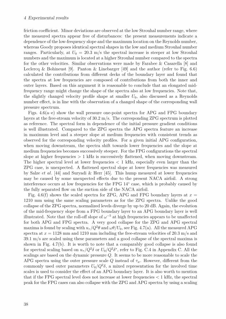
searchers. Of particular interest is the modeling of the one- and two-point statisticsrelevant to the structural excitation. Goody [36] proposed an empirical one-point wallpressure spectral model for ZPG boundary layers. The model was derived based on themeasured spectra by seven different experiments. Taking advantage of self-similarity of themeasured spectra, a spectral formulation is built by an increase with ω2 at low frequencies,a decrease with approximate ω−0.775 at medium frequencies and a rapid drop with ω−5 athigh frequencies. A highlight of this model is that the change of the mid-frequency spectralextension due to the Reynolds number effect was considered by introducing a timescalefactor.In practice, non-ZPG flows are of more interest. Recently, more studies concentrating
on effects of the pressure gradient on the wall pressure fluctuations have been conducted.Rozenberg [46] analyzed the different spectral features between the boundary layer under aZPG and an APG based on some selected experimental and numerical results, and showedthat a large inaccuracy in the spectral prediction occurs if the Goody model is applied foran APG case. Therefore, modeling of the wall spectrum for the APG boundary layer isof particular interest. It is, however, a difficult task. One major reason is because self-similarity of wall pressure spectra under APGs does not exist even approximitely. Basedon the observation that an APG increases the spectral peak level and the spectral dropin the mid-frequency range compared to the ZPG case, Rozenberg modified the Goodymodel involving some boundary layer parameters, e.g. boundary layer thickness basedparameters and Clauser’s equilibrium parameter, to capture the spectral changing trenddue to the presence of the pressure gradient. Later, other one-point spectral models forAPG boundary layers were proposed by Kamruzzaman et al. [47] and Catlett et al. [48]based on the similar concept.To predict the feature of wall-pressure two-point statistics, Corcos [51] found that self-
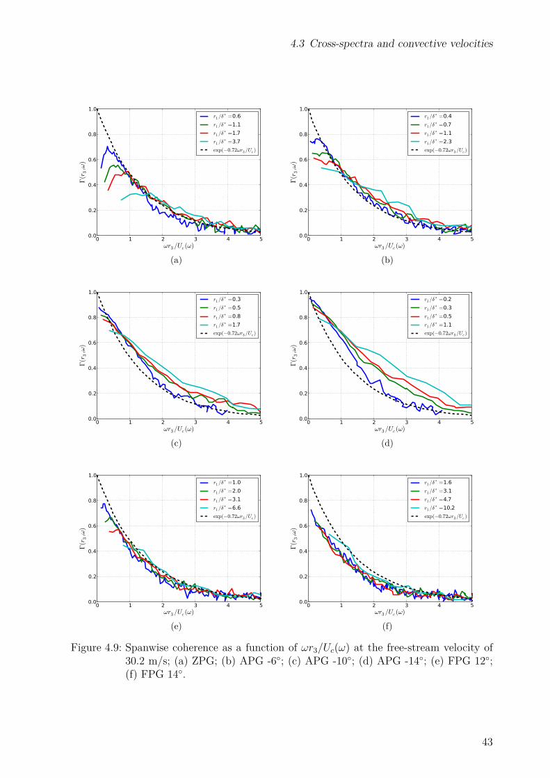
similarity also exists for the spectral coherence in both streamwise and spanwise directionsand the coherence at different distances in each direction can be well described by a singleexponential function, e.g. exp(−α|ωr1/Uc|), where α is an empirical constant and r1 isthe streamwise distance. Based on this observation, a cross-spectral model was proposed.The model involves a constant in each exponential function to define the rate of the de-correlation, which needs to be determined empirically. So far, the experimental resultsfrom the literature indicated that the value of the constant for the streamwise directiondepends on the Reynolds number, whereas for the spanwise direction it does not. Notethat, due to the formulation of the exponential function, the coherence approaches unitywhen the distance between two points or the spectral frequency is close to zero. However,it is the case only when the distance approaches zero. Experimental results [6, 8, 9] showedthat the coherence drops at low frequencies and this also means the Corcos model cannotpredict accurately the coherence in the low-frequency range. This feature of decreasingcoherence at low frequencies was reproduced by the theoretical work from Chase [30],
6
1.3 Scope and objectives
who calculated the wall pressure features for both mean-shear and turbulence-turbulenceterms in the wavenumber domain with consideration of the effect of decaying convectiveturbulence.
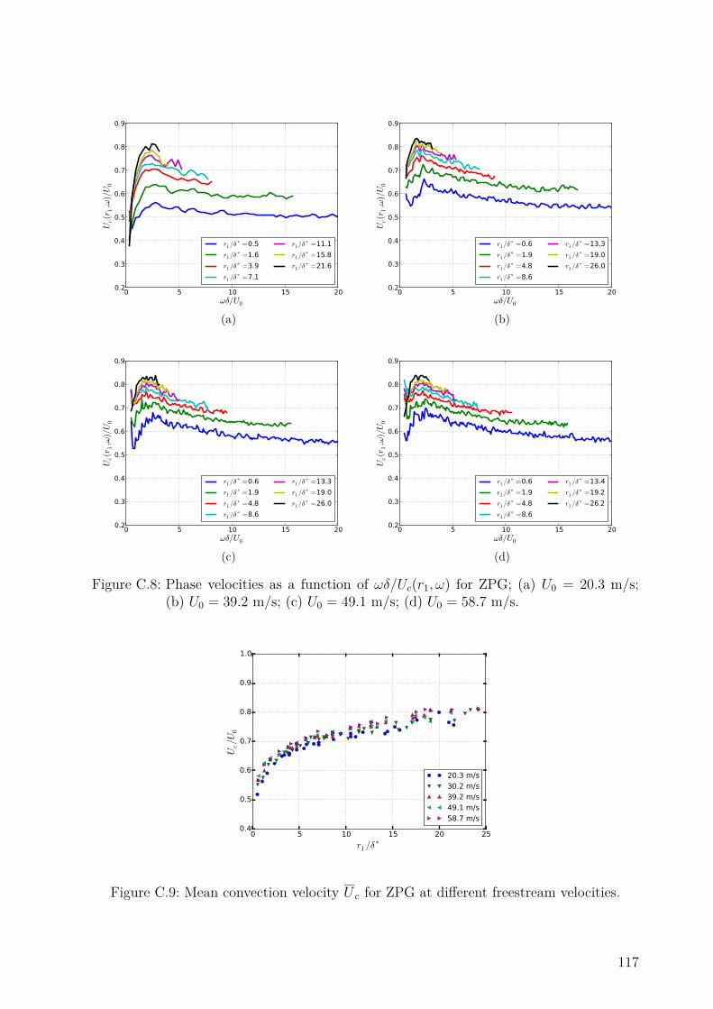
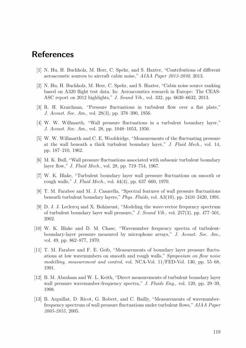
1.3 Scope and objectivesIn the present work, features of the wall pressure field are investigated experimentallyand numerically. A generic test setup is established in the Aeroacoustic Wind TunnelBraunschweig (AWB), which is able to generate both zero and non-ZPG turbulent bound-ary layers. Since, in reality, decelerated/accelerated flows occur most often and sincewall pressure fluctuations under non-zero pressure gradient flows have not been studiedas extensively as under zero pressure gradients, major efforts of the present experimentalinvestigation are made to study the effect of mean flow pressure gradients on wall pressurefluctuations.Wall pressure one- and two-point statistics (in the streamwise and spanwise directions)
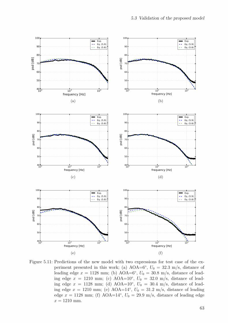
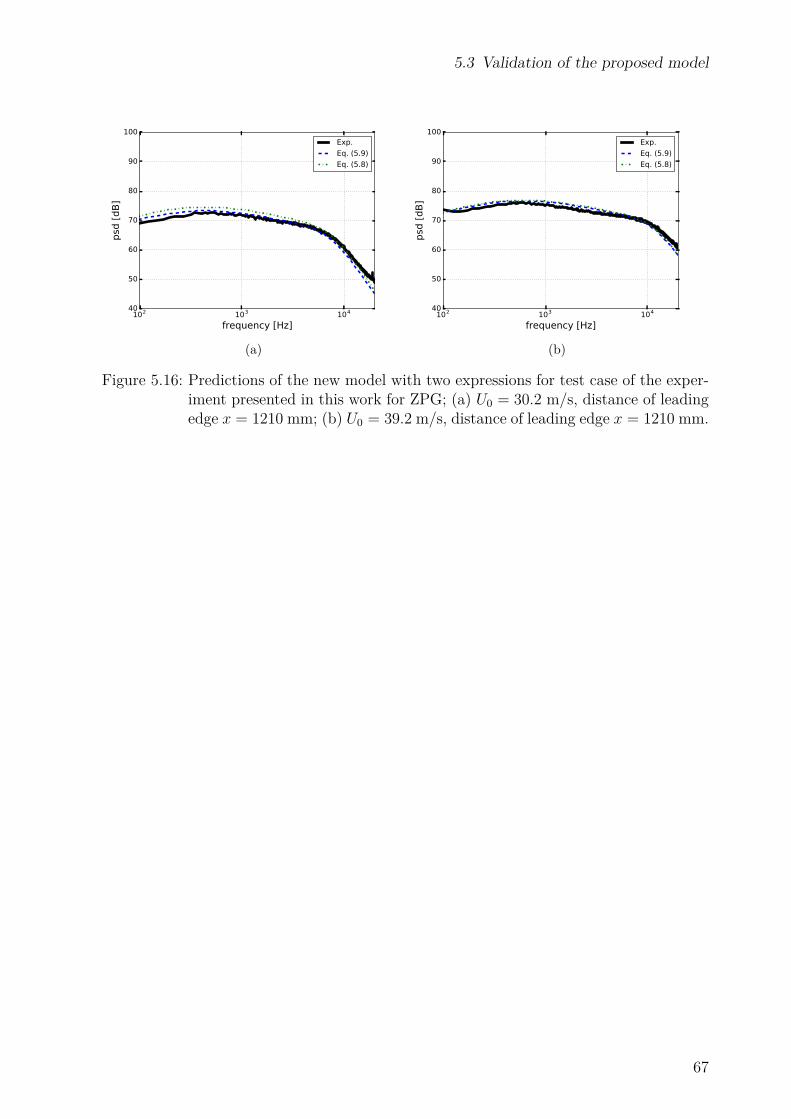
under zero and non-ZPG also including the respective flow properties within the boundarylayer are measured and studied. The effect of the pressure gradient on the boundary layermean velocity profile, on the wall pressure one-point spectra, on the wall pressure coherencein the streamwise and spanwise directions and on the wall pressure convection velocitiesare analyzed and discussed. The pressure gradient influences the boundary layer propertiesand consequently the features of the wall pressure fluctuations. The relationship betweenthe boundary layer properties and the wall pressure one-point spectra is investigated basedon the present experimental results. Furthermore, a spectral model to predict wall pressureone-point spectra under APGs (incorporating ZPGs) is proposed. The Goody model,which is suitable for ZPG cases, is used as the basis for developing the model. The basicconcept of the model is to use the boundary layer parameters to predict the spectral formdeparting from ZPG cases caused by presence of the pressure gradient. Predictions fromthe proposed model and other published models (for the APG cases) are made for fivetest cases at four different test facilities. Comparisons and assessments of the models aregiven.Another goal of the experiment is to establish a database as the validation basis for nu-
merical simulations. The numerical simulation is another means to investigate the featuresof the wall pressure fluctuations. As mentioned before, due to the extremely high com-putational resources required, the simulations are restricted to low and medium Reynoldsnumbers. A more efficient numerical procedure is developed in this work. A stochas-tic method is used to generate synthetic turbulence with prescribed features from whichpressure fluctuations are deduced. The approach enables the study of what effects thevariation of turbulence characteristics and key parameters have on the resulting turbulentwall pressure fluctuations. The relative efficiency of the approach enables the study ofhigh Reynolds numbers and the conduct of parametric studies.For an incompressible flow, the fluctuating pressure field can be expressed with the Pois-
son’s equation. The equation is solved in the present work by using a free-space Green’sfunction and solving the convolution with a spatial fast Fourier transform utilizing Hock-ney’s method [75]. Both the mean-shear and the turbulence-turbulence terms occurringon the right-hand side of the Poisson’s equation are considered in the present study. Fur-thermore, synthetic isotropic and also anisotropic turbulence are applied to calculate the
7
1 Introduction
pressure fluctuations.The present procedure aims not to resolve the smallest eddies present in the turbulent
boundary layer, since they are normally responsible for the high frequencies of the wallpressure spectra. For example, for most practical applications of flow-induced structuralvibration the high frequencies are irrelevant due to the poor transmission efficiency.The features for the wall pressure fluctuations are thoroughly analyzed and compared
with published results from the literature. Importance of both the mean-shear and theturbulence-turbulence terms for the wall pressure fluctuations and the effect of the tur-bulence anisotropy are discussed. Furthermore, simulations for the present experimentalcases are conducted. The numerical results for the wall pressure one- and two-point fea-tures are compared to the experimental results.
1.4 OutlineChapter 2 provides the necessary fundamentals on wall pressure fluctuations beneath tur-bulent boundary layers, consisting of the derivation and the solution of the Poisson’sequation for pressure fluctuations within the boundary layer and empirical models forone-point spectra and coherences. The experimental test setups, measurement techniquesand the applied numerical approach are described in Chapter 3. Experimental resultsare discussed in Chapter 4, mainly concentrating on the mean flow properties, the wallpressure one-point spectra, the cross-spectra and the convection velocities. Based on theexperimental results, a one-point spectral model for zero and APG cases is proposed inChapter 5. Also comparison with other exiting models is provided. In Chapter 6, simu-lated one-point spectra and two-point cross-correlations of wall pressure fluctuations areanalyzed in detail. The numerical approach is verified and validated by comparing withthe theoretical results and the experimental results from the literature and the presentexperiment. Conclusions and outlook are addressed in Chapter 7.
8
2 Fundamentals of wall pressure fluctuationsbeneath turbulent boundary layers
In this chapter, the fundamentals of the wall pressure fluctuations beneath turbulentboundary layers are provided. For an incompressible flow, the pressure fluctuations withinthe turbulent boundary layer can be determined by Poisson’s equation. A mathematicalderivation of Poisson’s equation and the analytical solution of it for the wall pressurespectrum contributed from the mean-shear term are given in section 2.1. Furthermore, abrief summary of the empirical models for prediction of the wall pressure spectrum andthe cross-spectrum are provided in section 2.2.
2.1 Theoretical approaches2.1.1 Poisson’s equation for pressure fluctuations within boundary
layersThe differential forms of the conservation equations for mass and momentum are
∂ρ
∂t+∇· ρu = 0 , (2.1)
∂ρu∂t
+∇· ρuu +∇p = ∇· τ , (2.2)
where ∇· is the divergence operator, ρ is fluid density, t is time, u is the flow velocityvector, p is pressure and τ is the deviatoric stress tensor. In terms of the pressure fluc-tuations, the deviatoric stress tensor τ is generally not relevant. Therefore, for deviationof Poisson’s equation to govern the pressure fluctuations within the boundary layer, τ isneglected.Taking the partial time derivative of Eq. (2.1) and the divergence of Eq. (2.2) and
neglecting of τ , the Eq. (2.1) and Eq. (2.2) become
∂2ρ
∂t2+∇· ∂ρu
∂t= 0 , (2.3)
∇· ∂ρu∂t
+∇·∇· ρuu + ∆p = 0 . (2.4)
Combining Eq. (2.3) and Eq. (2.4), we obtain
−∆p = ∇·∇· ρuu − ∂2ρ
∂t2. (2.5)
The density ρ may be split into a averaged mean part ρ and a fluctuating part ρ′,expressed as ρ = ρ + ρ′. We limit our discussion to a steady flow, i.e. ∂ρ/∂t = 0. Thus,Eq. (2.5) becomes
−∆p = ∇·∇· ρuu − ∂2ρ′
∂t2. (2.6)
9
2 Fundamentals of wall pressure fluctuations beneath turbulent boundary layers
Isentropy a20ρ′ = p′ applies approximately whenever the flow is cold and the Mach numbers
are subsonic as is true for all cases studied here. Here a0 denotes the speed of sound inthe medium, Eq. (2.6) can be written as
1a2
0
∂2p′
∂t2−∆p = ∇·∇· ρuu . (2.7)
Taking the time average of Eq. (2.7), we obtain
−∆p = ∇·∇· ρuu . (2.8)
The same as dealing with ρ, we split the pressure into p = p+p′ and put it into Eq. (2.7),reads
1a2
0
∂2p′
∂t2−∆p−∆p′ = ∇·∇· ρuu . (2.9)
Substituting Eq. (2.8) into Eq. (2.9),
1a2
0
∂2p′
∂t2−∆p′ = ∇·∇· (ρuu − ρuu) . (2.10)
We can also split the flow velocity into the density weighted time averaged (Favre-averaged) mean part and the fluctuating part, i.e. u = u + u ′′ with u = ρu/ρ. Thus, ρuuand ρuu can be expressed as
ρuu = ρ(u + u ′′)(u + u ′′) = ρ(uu + uu ′′ + u ′′u + u ′′u ′′) , (2.11)ρuu = ρuu + ρuu ′′ + ρu ′′u + ρu ′′u ′′ = ρ(uu + u ′′u ′′) . (2.12)
Putting the obtained expression for ρuu and ρuu into Eq. (2.10), we obtain
1a2
0
∂2p′
∂t2−∆p′ = ∇·∇·
(ρ(uu ′′ + u ′′u + u ′′u ′′ − u ′′u ′′) + ρ′(uu + uu ′′ + u ′′u + u ′′u ′′)
If we write Eq. (2.14) in a Cartesian coordinate system, it becomes
∆p′ = −ρ0
(2∂2uiu
′j
∂xi∂xj+∂2(u′iu′j − u′iu′j)
∂xi∂xj
). (2.15)
For a mean flow in the x1 direction and a well-developed quasi-parallel two-dimensional (2-D) incompressible turbulent boundary layer, i.e. ∂ui/∂xi = 0, u2,3 → 0 and ∂u1/∂x1,3 → 0,Poisson’s equation becomes
∆p′ = −ρ0
(2∂u1
∂x2
∂u′2∂x1
+∂2(u′iu′j − u′iu′j)
∂xi∂xj
). (2.16)
10
2.1 Theoretical approaches
2.1.2 Solutions to Poisson’s equationThe source term on the right-hand side of Eq. (2.16) comprises two parts. The firstpart is the mean-shear turbulence interaction term and the second part is the turbulence-turbulence interaction term. If the boundary is a rigid flat surface, the fluctuating pressurecan be calculated from the convolution of the free-space Green’s function of the Poisson’sequation with the right-hand side source term, i.e.,
p′(x, t) =∫
Vs+V′sQ(y, t) ·G(x− y) dV (y), (2.17)
where
Q(y, t) = −ρ0
(2∂u1
∂x2
∂u′2∂x1
+∂2(u′iu′j − u′iu′j)
∂xi∂xj
), (2.18)
G(x− y) = − 14π|x− y|
. (2.19)
In Eq. (2.17) the integration is carried out over the original source area Vs plus a sourcearea V′s that represents an image of Vs mirrored at the solid wall in order to realize theappropriate wall boundary condition (∂p/∂n)x2=0 = 0 of the pressure fluctuations [50].At the plane surface, the pressure fluctuations contributed from the virtual mirrored
source is identical to the one from the real source. Restricting the source term within theboundary layer and putting Eq. (2.19) into the Eq. (2.17), the expression for calculatingthe wall pressure fluctuations can be written as
p′(x1, 0, x3, t) = − 12π
∫δ
Q(y, t)r
dV (y), (2.20)
where r = |x− y| and δ denotes the boundary layer thickness. It is more convenientto analyze the stochastic wall pressure fluctuations in wavenumber-frequency domain bytaking three-dimensional (3-D) Fourier transform,
where k and xs are the wave vector and spatial vector in the surface plane, i.e. k = (k1, k3)and xs = (x1, x3). Substituting Eq. (2.20) into Eq. (2.21) and taking the Fourier transformwith respect to t, we obtain
p′(k, ω) = − 1(2π)3
∫δQ(y, ω)
∞∫−∞
∞∫−∞
exp (−ik · xs)r
dS(xs) dV (y). (2.22)
From the identity (refer to [50]),
12π
∞∫−∞
∞∫−∞
exp (−ik · xs + ik0r)r
dS(xs) =i exp
(iy2
√k2
0 − k2)
exp(−ik · ys)√k2
0 − k2, (2.23)
where |k| = k =√k2
1 + k23, k0 = ω/a0 and ys = (y1, y3), Eq. (2.22) for a0 →∞ and k0 = 0
becomes,p′(k, ω) = − 1
(2π)2
∫δQ(y, ω)exp(−ky2) exp(−ik · ys)
kdV (y). (2.24)
11
2 Fundamentals of wall pressure fluctuations beneath turbulent boundary layers
UsingQ(k, ω) = 1
(2π)2
∫δQ(y, ω) exp(−ik · ys) dV (y), (2.25)
Eq. (2.24) finally yields,
p′(k, ω) = −δ∫
0
Q(k, ω)exp(−ky2)k
dy2. (2.26)
The source term Q consists of two parts, i.e. the mean-shear term and the turbulence-turbulence term,
Q = Qms +Qtt, (2.27)where
Qms = −2ρ0∂u1
∂x2
∂u′2∂x1
, (2.28)
Qtt = −ρ0∂2(u′iu′j − u′iu′j)
∂xi∂xj. (2.29)
Since the Poisson’s equation is linear, the mean-shear term and the turbulence-turbulenceterm can be separately solved, thus,
p′ms(k, ω) = −δ∫
0
Qms(k, ω)exp(−ky2)k
dy2, (2.30)
p′tt(k, ω) = −δ∫
0
Qtt(k, ω)exp(−ky2)k
dy2. (2.31)
The source term for the mean-shear term follows,
Qms(k, ω) = 1(2π)2
∞∫−∞
∞∫−∞
Qms(ys, ω) exp(−ik · ys) dS(ys). (2.32)
Combining with Eq. (2.28), Eq. (2.32) becomes
Qms(k, ω) = −2ρ0∂u1
∂x2
1(2π)2
∞∫−∞
∞∫−∞
∂u′2∂x1
(ys, ω) exp(−ik · ys) dS(ys) (2.33)
= −2ρ0∂u1
∂x2ik1u
′2(k, ω). (2.34)
The same process for the turbulence-turbulence terms, the terms becomeQtt11(k, ω) = ρ0k
21u′1u′1(k, ω), (2.35)
Qtt12(k, ω) = −ρ0ik1∂u′1u
′2
∂x2(k, ω), (2.36)
Qtt13(k, ω) = ρ0k1k3u′1u′3(k, ω), (2.37)
Qtt22(k, ω) = −ρ0∂2u′2u
′2
∂x2∂x2(k, ω), (2.38)
Qtt23(k, ω) = −ρ0ik3∂u′2u
′3
∂x2(k, ω), (2.39)
Qtt33(k, ω) = ρ0k23u′3u′3(k, ω). (2.40)
12
2.1 Theoretical approaches
For the mean-shear term, an analytical solution can be derived. Combining Eq. (2.30)and Eq. (2.34), the pressure fluctuations contributed from the mean-shear term can becalculated with
p′ms(k, ω) =δ∫
0
2ρ0∂u1
∂x2ik1u
′2(k, ω)exp(−ky2)
kdy2. (2.41)
Using Eq. (2.41), the wall pressure spectrum for the mean-shear term can be derived as
where R22(y2 − y′2) represents the correlation for the velocity fluctuations u′2 between thewall-normal positions y2 and y′2. By integrating R22(y2− y′2) in the wall-normal direction,we obtain the integral length scale Λ22,
Λ22(y2) =δ∫
0
R22(y2 − y′2) dy′2. (2.45)
Integrating over y′2 and with the help of Eqs. (2.44–2.45) and an approximation of R22(y2−y′2) = Λ22(y2, y
′2)δ(y2 − y′2), the solution of the wall pressure spectrum for the mean-shear
where Φ22(y2, k1, k3) is the velocity wavenumber spectrum, Uc denotes the eddy convectivevelocity and φm(ω−Uck1) is the so-called moving axis spectrum, e.g. for frozen turbulenceφm(ω−Uck1) = δ(ω−Uck1). Taking integration of Eq. (2.46) in the wavenumber domainand combining Eq. (2.47), we obtain the solution for the spectrum Φppms(ω)
Φppms(ω) = 4ρ20
δ∫0
∞∫−∞
∞∫−∞
k21k2 exp(−2ky2)
[∂u1(y2)∂x2
]2
Φ22(y2, k1, k3)
φm(ω − Uck1)Λ22(y2) dk1dk3dy2. (2.48)
With this expression, the wall pressure spectrum Φppms(ω) contributed from the mean-shear term can be evaluated if the parameters δ, ∂u1(y2)/∂x2, Φ22(y2, k1, k3), φm(ω−Uck1)and Λ22(y2) are provided. However, only the boundary layer thickness δ and the wall-normal gradient of the mean velocity u1 can be easily measured or estimated by RANS
13
2 Fundamentals of wall pressure fluctuations beneath turbulent boundary layers
calculations. The other parameters are hard or not possible to measure, which are usuallyestimated by assumptions. Note that, the result of the wall pressure spectrum is influencedby the following factors: 1, the integral area, which is generally defined by the boundarylayer thickness δ; 2, the gradient of the mean velocity profile ∂u1(y2)/∂x2, i.e. the shapeof the mean velocity profile; 3, the wavenumber velocity spectrum Φ22(y2, k1, k3); 4, themoving axis spectrum φm(ω − Uck1), i.e. decay of the convective eddies; 5, the integrallength scale Λ22(y2). And following influences of these factors can be summarized: 1, athicker δ can lead to a larger pressure spectral level; 2, a different boundary layer profileshape may change the shape of the wall pressure spectrum and also the locations of thesource weighting for the wall pressure fluctuations. This indicates that the wall pressurespectral shape of zero or non-zero pressure gradient boundary layers could be different; 3,an increase of the intensity of the velocity fluctuations Φ22 will increase the spectral leveland a different shape of the spectrum Φ22(y2, k1, k3) may influence of the wall pressurespectral shape; 4, the moving axis spectrum φm(ω−Uck1) represents the turbulence decayduring convection and combines the spectrum in the wavenumber domain and in thefrequency domain, e.g. for a frozen turbulence k1 = ω/Uc. The spectrum of φm will affectthe distribution of the energy and consequently the shape of the wall pressure spectrum; 5,an increase of the length scale Λ22(y2) will increase the spectral level and also impacts thespectrum of Φ22(y2, k1, k3), which can shift the energy from a higher wavenumber regionto a lower wavenumber region.
2.2 Empirical model approaches2.2.1 One-point spectral modelSpectral model for zero pressure gradient boundary layers
Prediction of the wall pressure spectra is of great practical interest. Many spectral models[32, 30, 76, 34, 35, 36, 37] for zero pressure gradient (ZPG) boundary layers were proposed.The most used one is Goody’s model [36], which is briefly summarized below in thissection. Goody utilized self-similarity of wall pressure fluctuation spectra induced byZPG boundary layers and incorporates Reynolds number effects in the high frequencyrange with a time scale ratio RT , expressed as
Φ(ω)Ueτ 2wδ
= a· (ωδ/Ue)b
[(ωδ/Ue)c + d]e + [fRgT · (ωδ/Ue)]h
, (2.49)
where Ue is the boundary layer edge velocity, defined as 0.99U0 (U0 is the local free-streamvelocity). The value of parameters a− h was obtained by fitting measurement data fromthe literature, a = 3, b = 2, c = 0.75, d = 0.5, e = 3.7, f = 1.1, g = −0.57 and h = 7. Theycontrol the shape of the non-dimensional spectrum. The formulated spectrum has threedifferent regions with different spectral slopes. The spectrum increases at low frequencies,decreases at medium frequencies and rolls off rapidly at high frequencies. The spectralslopes in the different frequency ranges are driven by a combination of b, c, e and h. Theparameter b fixes the slope at low frequencies, the function c· e−b is in charge of the slopeat medium frequencies and h−b at high frequencies. The formulated spectrum of Goody’smodel has a shape with a slope of ω2 at low frequencies, ω−0.775 at medium frequenciesand ω−5 at high frequencies. The spectral amplitude is adjusted by the value of a. The
14
2.2 Empirical model approaches
parameters f , g combined with RT determine the extension of the mid-frequency range,e.g. a larger RT corresponds to a longer extension of the slope at medium frequencies intohigher frequencies. The spectral peak location is affected by the value of d.
Spectral model for adverse pressure gradient boundary layers
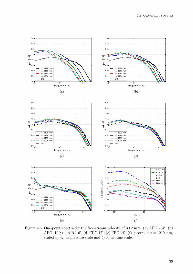
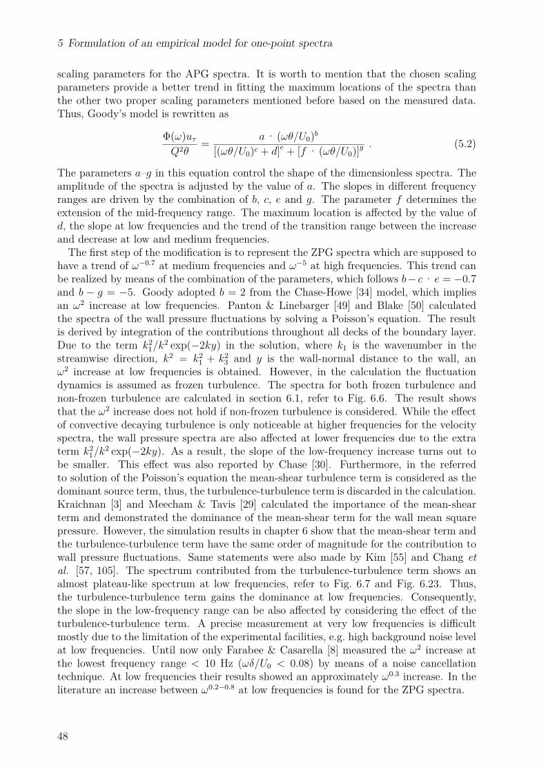
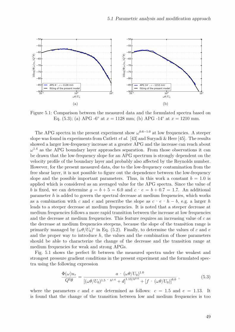
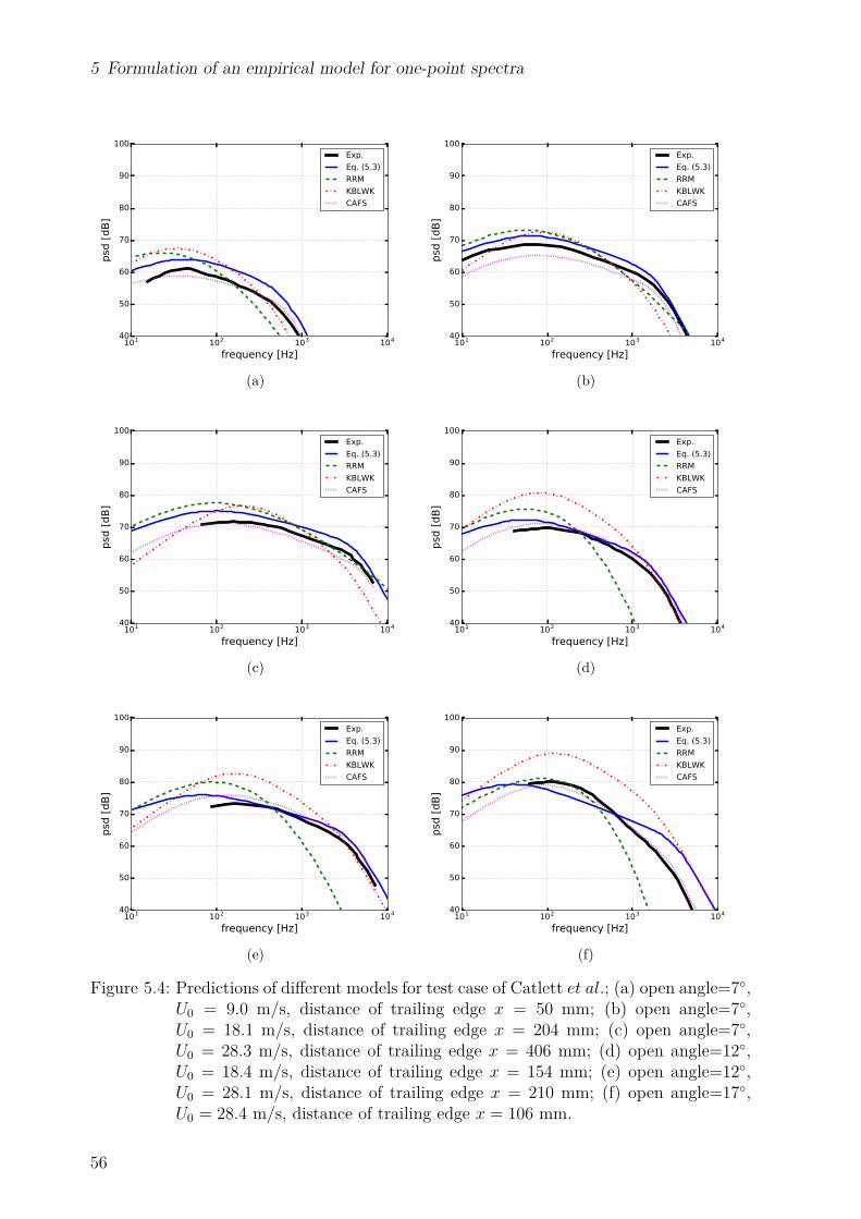
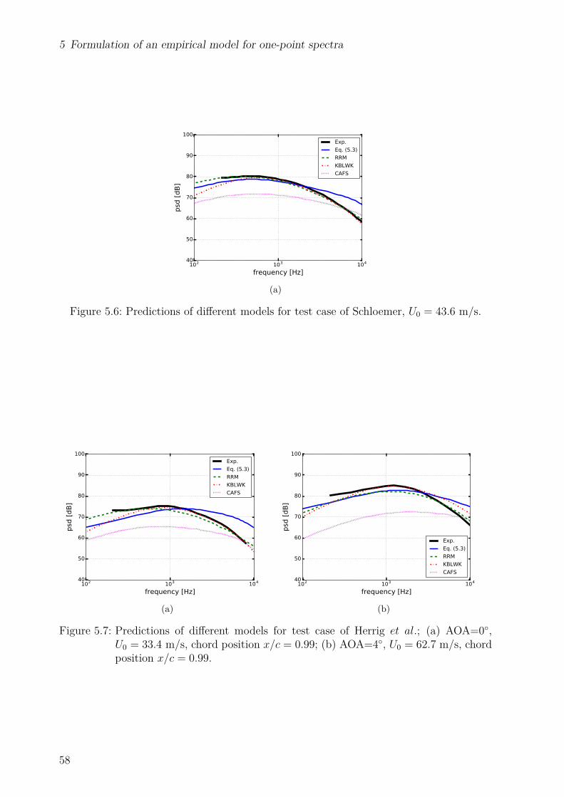
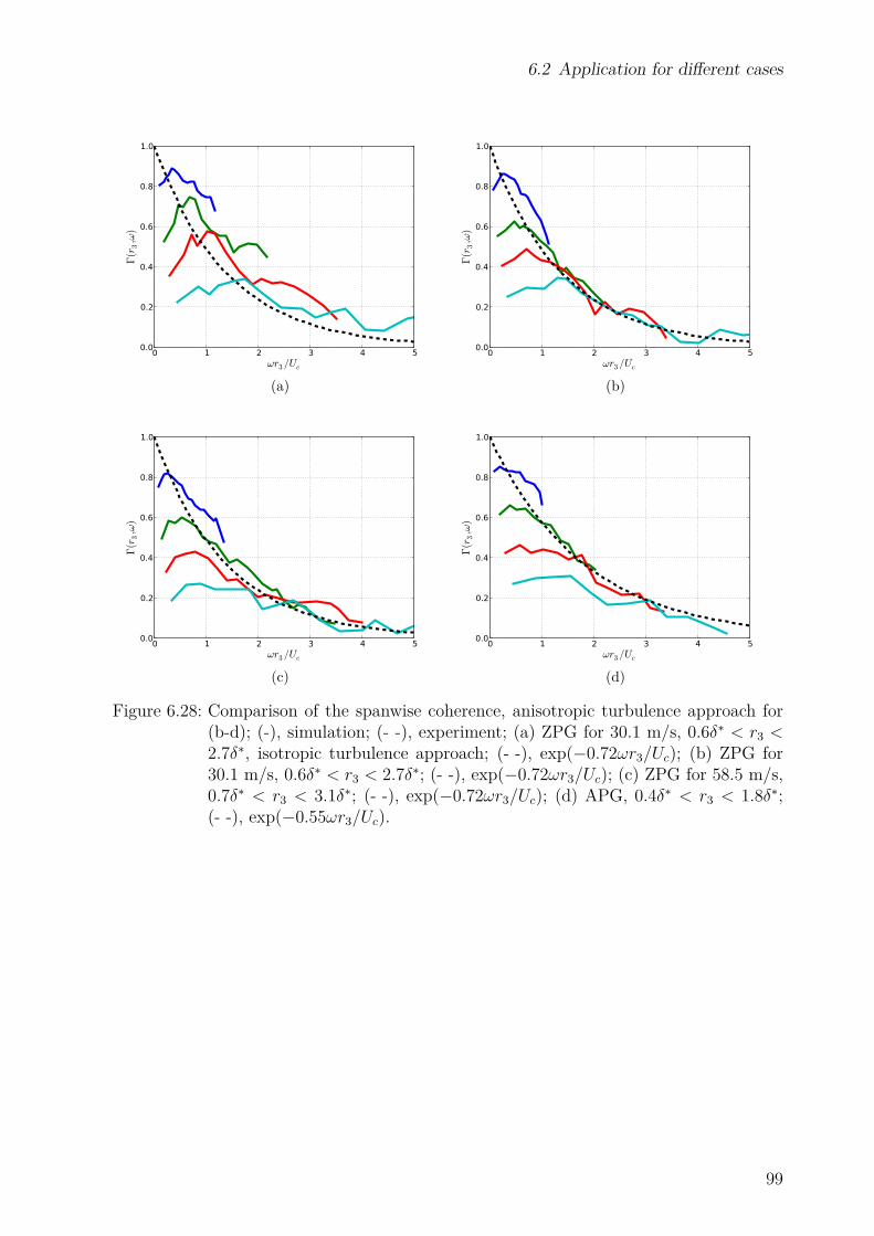
The wall pressure spectra induced by non-ZPG boundary layers become more complicatedand can not be well predicted by Goody’s model. Experimental studies [38, 39, 40, 41,42, 43, 44, 45] for pressure gradient effects on wall pressure fluctuations showed that thewall pressure spectra lose their self-similarity. A group of sensors was installed at differentstreamwise positions to measure the spectral development due to the impact of pressuregradients [43, 45]. For adverse pressure gradient (APG) boundary layers, the spectralslope at medium frequencies becomes successively steeper moving downstream. This isbecause the boundary layer development is influenced by the APG for a longer distanceat downstream positions. Furthermore, the stronger the pressure gradient, the steeper themid-frequency slope is.Several empirical models for APG boundary layers were proposed to predict the changing
trends from ZPG to APG boundary layers. A brief summary of the published spectralmodels for APG boundary layers is provided below.Rozenberg et al. [46] (RRM) analyzed the spectral variation between ZPG and APG
boundary layers from some experimental and numerical results and summarized the chang-ing trends through a combination of boundary layer characteristic parameters. Based onthe basic form of Goody’s model, an empirical spectral model including APG effects wasproposed by Rozenberg et al. [46], expressed as
Clauser’s equilibrium parameter βθ [77] is used to manage the slope variation at mediumfrequencies, the larger the value of βθ, the steeper the slope. The formulated spectrumshifts to a higher frequency and a larger amplitude as ∆δ/δ∗ increases. Both βθ and ∆δ/δ∗
are in charge of the spectral amplitude.Kamruzzaman et al. [47] (KBLWK) proposed a spectral model for the prediction of the
airfoil trailing edge noise. The wall pressure fluctuation spectra as measured by differentinvestigators [42, 78, 79, 80, 81, 82] were used to develop the model. The formulation ofthe model reads
2 Fundamentals of wall pressure fluctuations beneath turbulent boundary layers
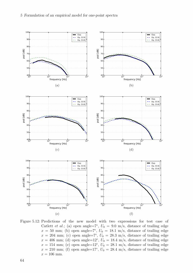
where βδ∗ = δ∗/τw · dp/dx, in which dp/dx represents the pressure gradient in the stream-wise direction, Πδ∗ = 0.8 · (βδ∗ + 0.5)3/4 and m = 0.5 · (H/1.31)0.3. Except for the mid-frequency extension determined by RT , the formulated spectrum has a constant shape fordifferent pressure gradient configurations, i.e. a constant decreasing slope of approximatelyω−2 at medium frequencies and a constant spectral peak location at the non-dimensionalfrequency. The spectral amplitude is adjusted by a combination of Clauser’s equilibriumparameter βδ∗ [83], Cole’s wake parameter Πδ∗ [84, 85] and boundary layer shape factorH.Catlett et al. [43, 48] (CFAS) measured the wall pressure fluctuations on tapered trailing
edge sections of a flat plate with three different opening angles and proposed an empiricalspectral model based on the measured data, which reads
where βδ,∆ = (δ,∆)/Q· dp/dx, Reδ,∆ = (δ,∆)Ue/ν and ∆ = δ∗√
2/Cf . The parametersa−h are derived by fitting to the measured spectra. The constants aG−hG from Goody’smodel with correspondent positions in Eq. (2.52) are replaced with the functions basedon boundary layer parameters, except for b = 2, which stands for an ω2 increase at lowfrequencies. The spectral amplitude, peak location and slope at medium frequencies areaffected by Clauser’s equilibrium parameter and Reynolds numbers defined with differentlength scales.
2.2.2 Cross-spectral modelThe combined spatio-temporal properties of the wall pressure fluctuations are also impor-tant features in terms of the flow-induced surface vibration. The space-time correlationfor the wall pressure fluctuations over (x1, x3) plane is defined by,
Rpp(x, r, τ) =< p′(x, t)p′(x + r, t+ τ) > (2.53)
where x = (x1, x3) and r = (r1, r3). Rpp(x, r, τ) denotes the correlation at the surfacepoint (x1, x3). If the wall pressure fluctuation field can be treated as a homogeneous field,so the correlation is not location-dependent, Rpp(x, r, τ) ∼ Rpp(r, τ). This assumption iswell fulfilled for fully developed 2-D turbulent boundary layers at high Reynolds numbers.Thus, the cross-spectrum can be defined by
Φpp(r1, r3, ω) = 12π
∞∫−∞
Rpp(r1, r3, τ) exp(−iωτ) dτ, (2.54)
16
2.2 Empirical model approaches
The most used model for describing the spatial and temporal properties of the wallfluctuating pressure field is the one proposed by Corcos [51]. He chose a separation formto model the cross-spectrum also regarding the convecting effects of the fluctuating field,expressed as
where Φpp(ω) is the wall pressure one-point spectrum, A(ωr1/Uc) and B(ωr3/Uc) representthe coherence function for the streamwise and spanwise directions and exp(iωr1/Uc) de-notes the phase difference due to the (passive) convection of the fluctuating field. Corcosfound similarity of the coherences in both streamwise and spanwise directions, and thecoherences can be well expressed by using exponential functions. Thus, the formulationof Corcos’s model reads
where α and β are empirical constants which can be determined from the measurement.The values of α and β represent the loss in coherence of the wall pressure fluctuations in thestreamwise and spanwise directions, respectively. A larger value implies a stronger decay.From the literature, we found 0.1 < α < 0.15 for ZPG boundary layers on a smooth surface.The value is Reynolds number dependent. Generally, for a larger Reynolds number thevalue of α is rather smaller, which may indicate the decay of the pressure fluctuation fieldis smaller. The turbulent flow on a rough surface causes a stronger turbulence decay inthe streamwise direction, which leads to a larger value of α = 0.32 measured by Blake [50].The decay is also larger for APG boundary layers. The stronger the pressure gradient, thelarger the value of α [48]. In contrast, for a favorable pressure gradient (FPG) boundarylayer, the value tends to be smaller. The value of β implies the size of the correlatedstructure in the spanwise direction. The value of β is found around β = 0.7 − 0.72.There is no evidence found that the value is dependent on the Reynolds number. ForAPG boundary layers, the value tends to be smaller which indicates a larger correlatedstructure in the spanwise direction.The coherence for the wall pressure fluctuations is defined by,
Note that, in this expression the coherence approaches 1 when r1,3 → 0 or ω → 0. The firstcondition r1,3 → 0 indicates that a closer distance has a larger coherence and the coherencebetween the same position is equal to 1. This is verified by the definition of the coherence,according to Eq. (2.57). The second condition ω → 0 indicates that the coherence increasesas the frequency decreases. This is true for the higher frequencies, where the similarity of
17
2 Fundamentals of wall pressure fluctuations beneath turbulent boundary layers
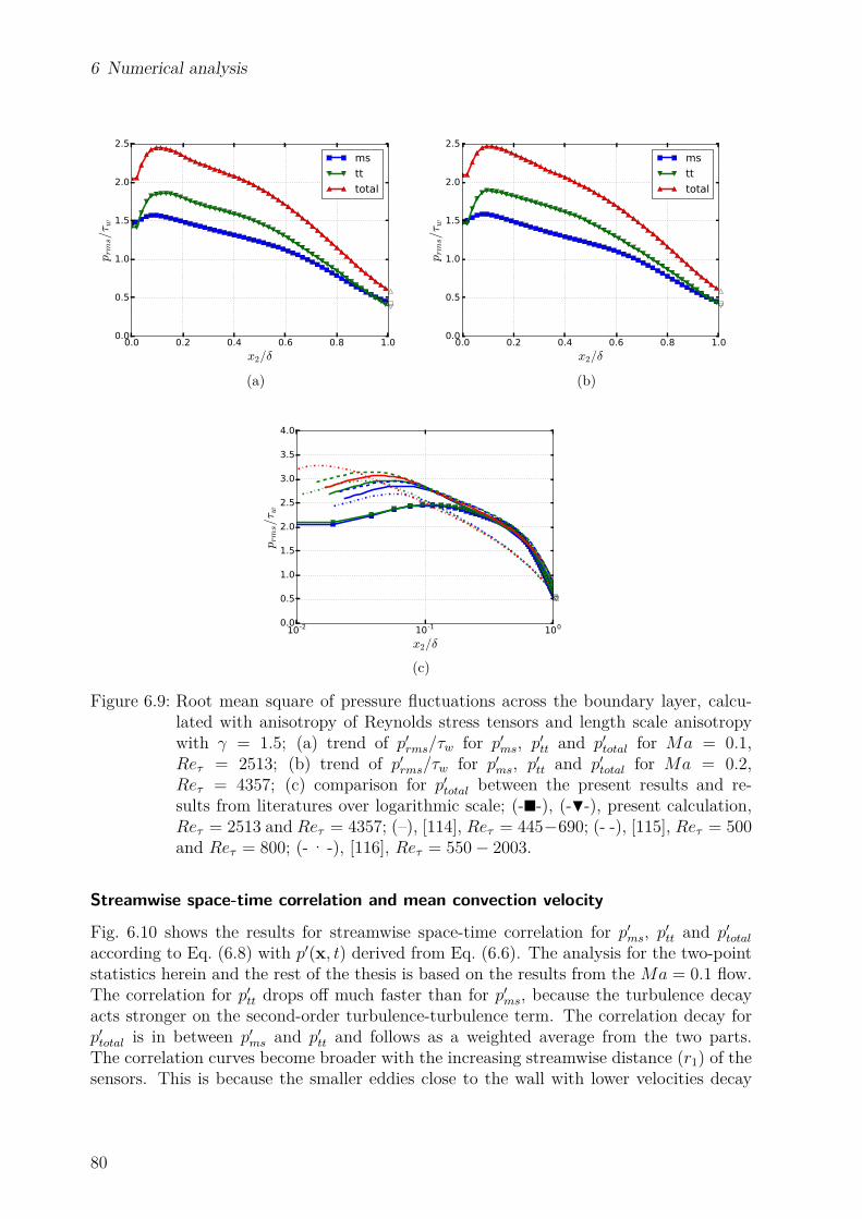
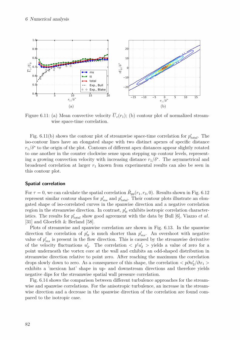
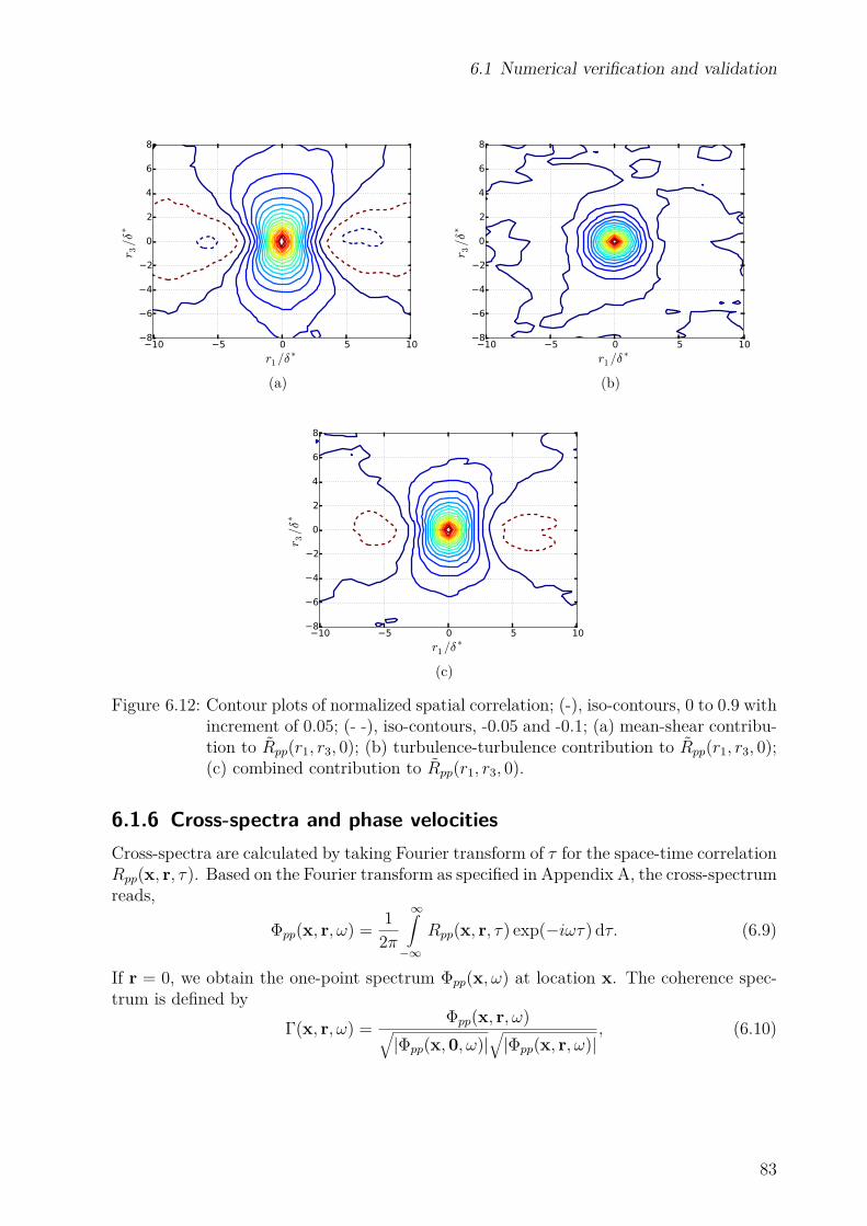
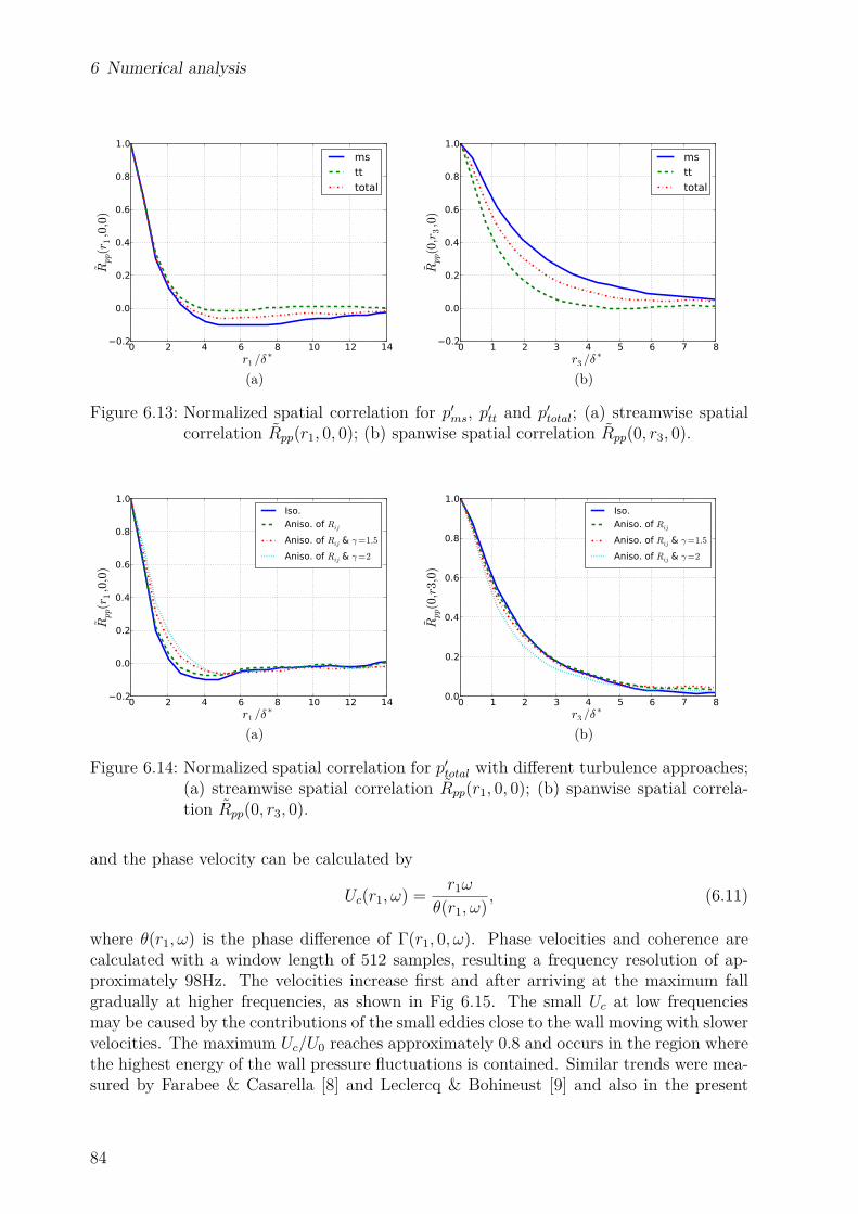
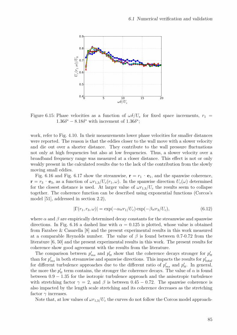
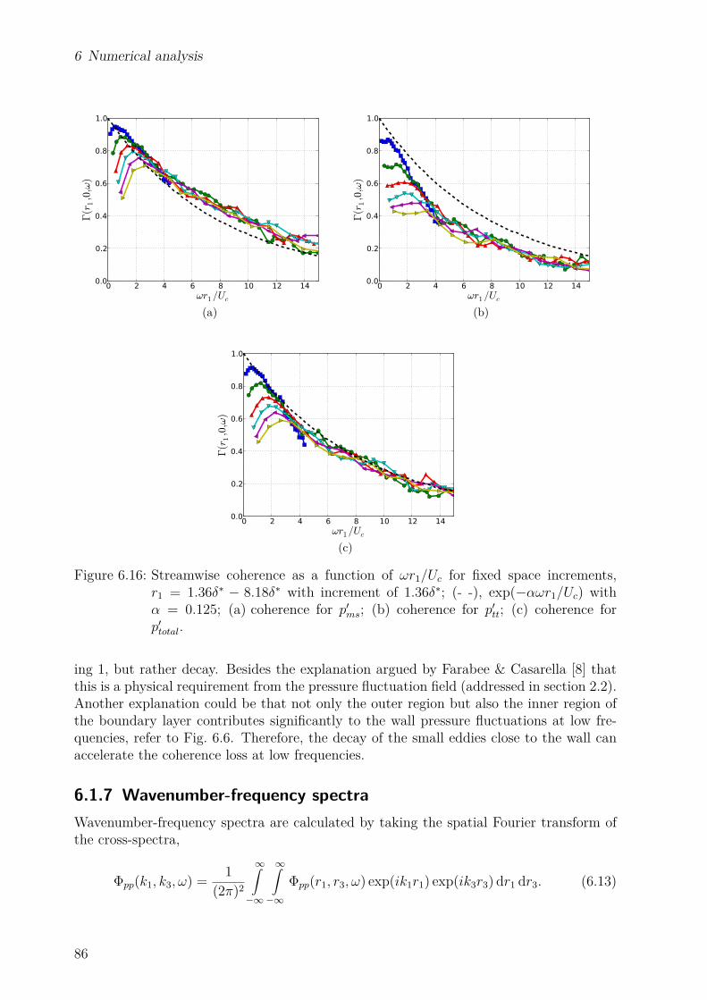
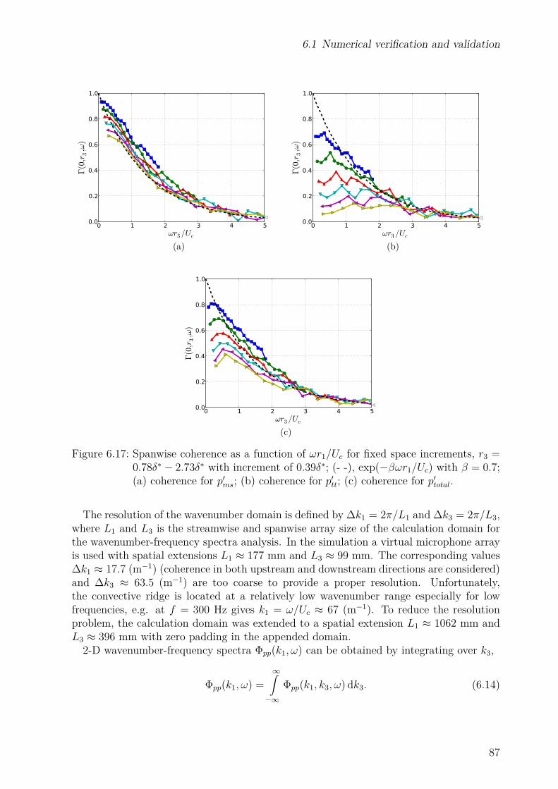
the coherence holds. Measurements [6, 8, 9] showed that a loss in similarity occurs at lowfrequencies and the coherence decreases consequently. Farabee & Casarella [8] argued thatthe decrease in the coherence is a physical requirement, otherwise, the eddies could producelow-frequency fluctuations which would convect without decay over an infinite distance.A cutoff frequency for the coherence is found located between 1.3 < ωδ/Uc < 2.7. Thecutoff frequency decreases as the distance r1 increases. A noteworthy finding is that thecutoff frequency occurs at the region where the spectral maximum of the wall pressurefluctuations is located. This may indicate that the lowest-decay eddies contribute the mostto the wall pressure fluctuations.
18
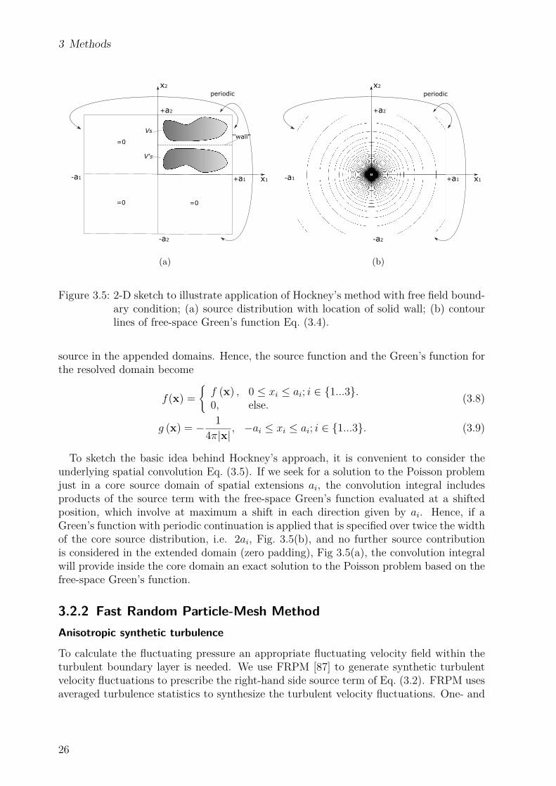
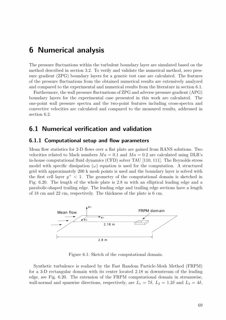
3 MethodsThe characteristics of wall pressure fluctuations beneath turbulent boundary layers wereexperimentally and numerically investigated. Experiments were conducted at a flat platemodel in the Aeroacoustic Wind Tunnel Braunschweig (AWB) [86]. Effects of the pressuregradients on the characteristics of the wall pressure fluctuations were studied by installingan adjustable National Advisory Committee for Aeronautics (NACA) 0012 airfoil witha chord length of 40 cm above the flat plate. The static wall pressure was measuredin the streamwise and spanwise directions on the plate model by static pressure ports.The dynamic wall pressure was measured by an ’L-shaped’ array of subminiature Kulitepressure transducers. In addition, the mean velocity profiles and the Reynolds stresstensors within the turbulent boundary layer were obtained using hot wire anemometers.Details of the test setups and the measurement techniques are described in section 3.1.The wall pressure fluctuations are obtained by solving Poisson’s equation. The source
terms on the right-hand side of the Poisson’s equation including the mean-shear and theturbulence-turbulence terms are realized using synthetic isotropic and anisotropic turbu-lence generated by the Fast Random Particle-Mesh Method (FRPM) [87]. The averagedturbulence statistics needed for the stochastic realization is provided by the Reynolds av-eraged Navier-Stokes (RANS) calculation. Anisotropy of the turbulence length scales canbe applied using different integral length scales in different directions. Reynolds stressanisotropy can be gained by using a scaling tensor for the relation between the anisotropicstress provided by the RANS calculation and the respective isotropic expression for theReynolds stress. The Poisson’s equation is solved by using the convolution theorem inthe wavenumber domain with a free-space Green’s function. For an exact realization ofthe Green’s function in conjunction with a Fourier transform method on a finite domain,Hockney’s method [75] is applied to the Poisson problem. A brief description of the appliednumerical method is provided in section 3.2.
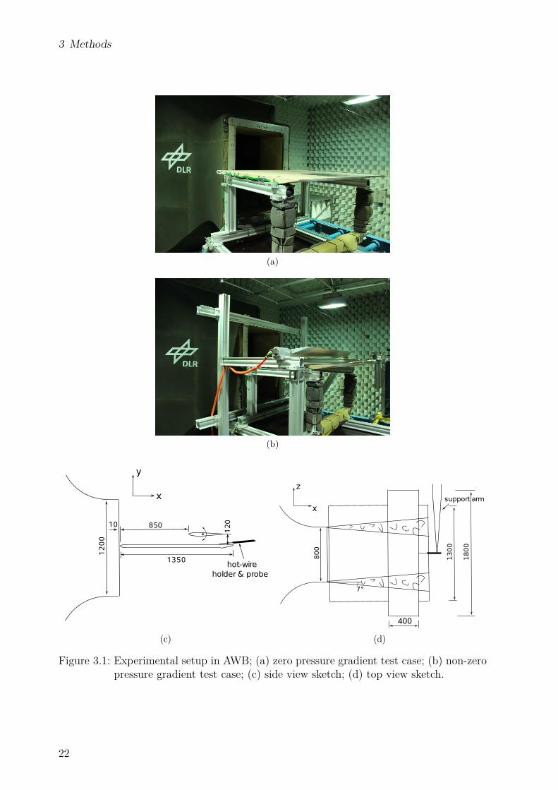
3.1 Experimental test cases3.1.1 Test setupsThe wall pressure fluctuations beneath a turbulent boundary layer with zero and non-zeropressure gradients were measured at a plate model in the open-jet anechoic test section ofthe AWB. Details of the experimental setup are documented in Fig. 3.1. A flat woodenplate was placed 10 mm downstream of the nozzle exit in the nozzle mid-height position.The plate surface was aligned with the flow direction.To design the plate model, following considerations were made. The background noise
of the AWB increases significantly at low frequencies < 300 Hz [86], which may disturb thelow frequency range of the wall pressure spectra, especially for higher flow velocities. Inorder to measure at least the maximum of the wall pressure spectra without disturbances,the spectral maximum should be located at > 300 Hz. Considering a thicker boundarylayer thickness for adverse pressure gradient (APG) boundary layers and the respective
19
3 Methods
frequency shift for the spectral maximum to lower frequencies, the maximum for the zeropressure gradient (ZPG) boundary layers should be located at much larger than 300 Hz,especially for higher flow velocities. The maximum position for the ZPG boundary layerscan be estimated based on ωmaxδ/Ue ≈ 2 [36], where ωmax denotes the angular frequencyof the spectral maximum, δ is the boundary layer thickness and Ue is the boundary layeredge velocity. For example, for a given velocity the thicker the boundary layer thicknessis, the lower the maximum frequency is. For this reason, a very thick boundary layerthickness at the measurement position is not desired. On the other hand, the boundarylayer thickness at the measurement position should also be thick enough, so that the log-law region of the boundary layer can be resolved experimentally based on the availablemeasurement equipment, so that consequently, the wall shear stress can be well estimated.Summing up, a boundary layer thickness on the order of 2 cm satisfies the above criteria.A 2 cm boundary layer thickness denotes an approximate 4 mm log-law region, whichcan be well measured and determined. Meanwhile, the maximum is estimated located atabout 950 Hz for Ue = 60 m/s, which is much larger than the criterion 300 Hz. To developa boundary layer of 2 cm thickness on a flat plate, the needed length downstream fromthe plate nose can be estimated according to δ ≈ 0.37x/Re1/5
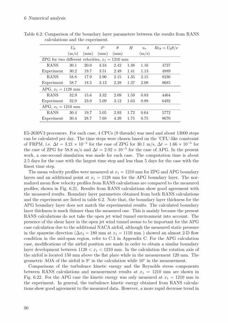
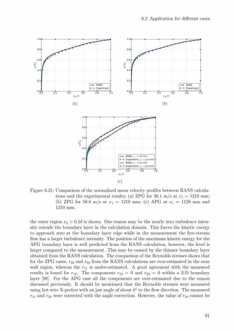
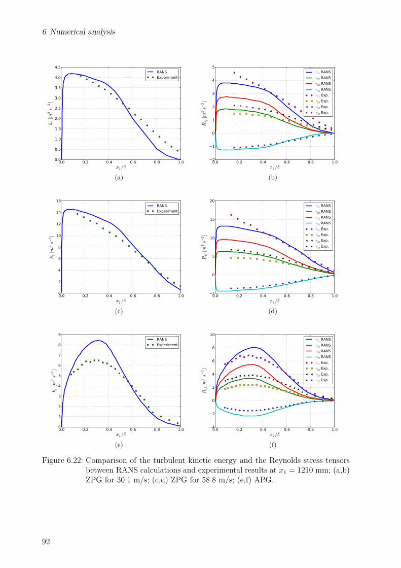
x [88], where x denotes thestreamwise distance away from the leading edge and Rex is the streamwise distance basedReynolds number. This results in a length of about 1.2 m. Furthermore, the measurementposition (about 1.2 m downstream of the leading edge of the plate) should be far enoughaway from the trailing edge of the plate, so that there is no disturbances from the trailingedge at the measurement position. On the other hand, to determine the Reynolds stress ofthe boundary layer, a crossed hot-wire placed parallel or with a possible small angle to theplate surface is required. This is because, to measure the spanwise velocity fluctuations,a yaw-angle in the wall-normal direction may induce measurement error and the errorcannot be corrected based on the yaw-angle calibration. Therefore, the distance betweenthe measurement position and the trailing edge of the plate is limited by the accessibledistance of the hot-wire probe away from the support arm of the traverse system (seeFigs. 3.1(b,d)), which is about 180 mm. This allows the support arm to be placed behindthe plate, which enables the hot-wire probe to be set with a small angle to the platesurface.The thickness of the plate should be large enough to ensure the setup is stable and allow
to insert the sensors and the cables. Thus, a length of 1350 mm and a thickness of 42 mmfor the plate model were chosen. The plate span is needed to be larger than the nozzle exitin order to prevent the interaction of the AWB open-jet shear layers between the top andbottom sides of the plate. The spreading angle of the free shear layer can be estimated atabout 7◦ [89]. The spreading angle of the shear layer on a plate may be larger than of afree shear layer. Thus, an angle of 10◦ was used to estimate the spreading distance of theshear layer at the trailing edge of the plate, which results in a distance of about 240 mm.Finally, a plate span of 1300 mm was determined, which is 250 mm wider than the nozzleexit on each side, see Fig. 3.1(d).A 125 mm long superellipse (n = 3) shaped leading-edge part was selected to avoid flow
separation [90] and manufactured by 3-D printing. Both sides of the plate were tripped at120 mm behind the leading-edge tip with 0.3 mm zigzag trip strips. A 12◦ beveled trailingedge on the bottom side of the plate was used to realize a ZPG turbulent boundary layeron the topside in the rear area [91]. The 5-mm thick trailing-edge tip was extended byfoam serrations to avoid vortex shedding and to reduce trailing-edge noise.
20
3.1 Experimental test cases
Pressure gradients were realized by placing an adjustable NACA 0012 airfoil with400 mm chord length and 1800 mm span width above the plate, see Fig. 3.1. The airfoilwas installed 120 mm above the plate relative to the wing’s chord at the geometric angleof attack (AOA) of 0◦. The rotation axis was at 41% of the chord length. The geometricAOA of the airfoil was varied between -14◦ and 14◦. The leading edge of the airfoil waslocated at x = 850 mm (x = 0 for the leading-edge tip of the plate). Both sides of theairfoil were tripped at 20% chord length with 0.4 mm zigzag trip strips to avoid a possiblelaminar vortex shedding noise originated at the large AOA.
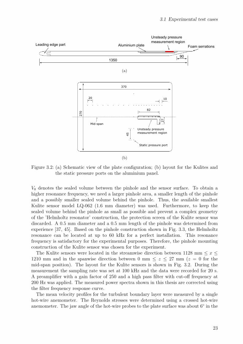
3.1.2 Measurement techniquesA 370 mm long, 270 mm wide and 5 mm thick aluminium panel equipped with 25 staticpressure ports and twelve Kulite pressure transducers was placed at mid-span in the rearportion of the plate, see Fig. 3.2. The rear edge of the panel was located at 90 mmupstream of the trailing edge of the plate. The static pressure ports (0.5 mm diameter)covered 290 mm in the streamwise direction and 180 mm in the spanwise direction.The wall pressure fluctuations were measured by twelve pinhole-mounted Kulite pressure
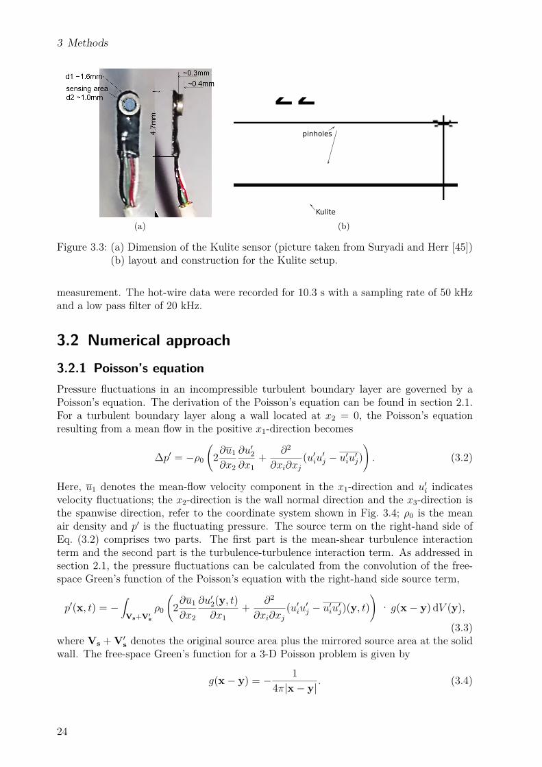
transducers without the protection screen, model LQ-062-0.35 bar. The diameter of thepinhole was 0.5 mm and the depth was 0.5 mm. The Kulite sensor with a diameter of1.6 mm was glued with silicone in a 1.8 mm diameter hole behind the pinhole. A photoand an installation sketch of the Kulite sensor is shown in Fig. 3.3.The selection of the Kulite sensor and the pinhole construction was determined based
on the following considerations. To measure the wall pressure fluctuations, two types ofmounting constructions, namely flush mounting and pinhole mounting, can be used.In general, for the flush mounting construction the sensor size is too large to measure
the wall pressure fluctuations at high frequencies. An attenuation of the measured wallspectra at high frequencies will be caused due to the finite sensor size. This is becausethe sensor measures an averaged pressure fluctuations over the whole sensor area, andthe higher the frequency is (smaller wave length), the stronger the attenuation is. Anoticeable attenuation of about 1 dB may occur at about ωr/Uc = 0.3, estimated basedon the Corcos correction [16], where r is the sensor radius and Uc is the convective velocityof the wall pressure fluctuations, which is usually estimated between Uc = 0.6 − 0.8U0.Thus, the frequency range without attenuation (<1 dB) for the wall pressure spectra canbe estimated for a given flow velocity and sensor size. The smallest available Kulite sensorhas a diameter of 1.6 mm with a so called ’B-screen’ (eight 0.2 mm diameter holes around a1.2 mm diameter circle), so the radius of the effective sensor area can be roughly estimatedto be 0.6 mm. For a flow velocity U0 = 60 m/s and Uc estimated at 0.7U0, the frequencyrange without attenuation is estimated to extend to about 3.3 kHz, which is too low toinvestigate the features of the wall pressure fluctuations. Therefore, the flush mountingconstruction was discarded.For the pinhole mounting construction, the key criterion is the Helmholtz resonance
frequency. It should be high enough to avoid its impact on the measured wall pressurespectra. The Helmholtz resonance frequency can be estimated by
fres = a0
2π
√S0
V0 ·L, (3.1)
where S0 and L denote the pinhole area and the length of the pinhole, respectively, and
21
3 Methods
(a)
(b)
1200
10 850
120
1350
x
y
hot-wire holder & probe
(c)
400
80
0
13
00
18
00
x
z
support arm
7°
(d)
Figure 3.1: Experimental setup in AWB; (a) zero pressure gradient test case; (b) non-zeropressure gradient test case; (c) side view sketch; (d) top view sketch.
22
3.1 Experimental test cases
Leading edge part Aluminium plate
Unsteady pressure measurement region
Foam serrations
135090
(a)
370
20 10
82
45
27
270
Unsteady pressure measurement region
Static pressure port
Mid-span
(b)
Figure 3.2: (a) Schematic view of the plate configuration; (b) layout for the Kulites andthe static pressure ports on the aluminium panel.
V0 denotes the sealed volume between the pinhole and the sensor surface. To obtain ahigher resonance frequency, we need a larger pinhole area, a smaller length of the pinholeand a possibly smaller sealed volume behind the pinhole. Thus, the available smallestKulite sensor model LQ-062 (1.6 mm diameter) was used. Furthermore, to keep thesealed volume behind the pinhole as small as possible and prevent a complex geometryof the ’Helmholtz resonator’ construction, the protection screen of the Kulite sensor wasdiscarded. A 0.5 mm diameter and a 0.5 mm length of the pinhole was determined fromexperience [37, 45]. Based on the pinhole construction shown in Fig. 3.3, the Helmholtzresonance can be located at up to 60 kHz for a perfect installation. This resonancefrequency is satisfactory for the experimental purposes. Therefore, the pinhole mountingconstruction of the Kulite sensor was chosen for the experiment.The Kulite sensors were located in the streamwise direction between 1128 mm ≤ x ≤
1210 mm and in the spanwise direction between 0 mm ≤ z ≤ 27 mm (z = 0 for themid-span position). The layout for the Kulite sensors is shown in Fig. 3.2. During themeasurement the sampling rate was set at 100 kHz and the data were recorded for 20 s.A preamplifier with a gain factor of 250 and a high pass filter with cut-off frequency at200 Hz was applied. The measured power spectra shown in this thesis are corrected usingthe filter frequency response curve.The mean velocity profiles for the turbulent boundary layer were measured by a single
hot-wire anemometer. The Reynolds stresses were determined using a crossed hot-wireanemometer. The jaw angle of the hot-wire probes to the plate surface was about 6◦ in the
23
3 Methods
(a)
pinholes
Kulite
(b)
Figure 3.3: (a) Dimension of the Kulite sensor (picture taken from Suryadi and Herr [45])(b) layout and construction for the Kulite setup.
measurement. The hot-wire data were recorded for 10.3 s with a sampling rate of 50 kHzand a low pass filter of 20 kHz.
3.2 Numerical approach3.2.1 Poisson’s equationPressure fluctuations in an incompressible turbulent boundary layer are governed by aPoisson’s equation. The derivation of the Poisson’s equation can be found in section 2.1.For a turbulent boundary layer along a wall located at x2 = 0, the Poisson’s equationresulting from a mean flow in the positive x1-direction becomes
∆p′ = −ρ0
(2∂u1
∂x2
∂u′2∂x1
+ ∂2
∂xi∂xj(u′iu′j − u′iu′j)
). (3.2)
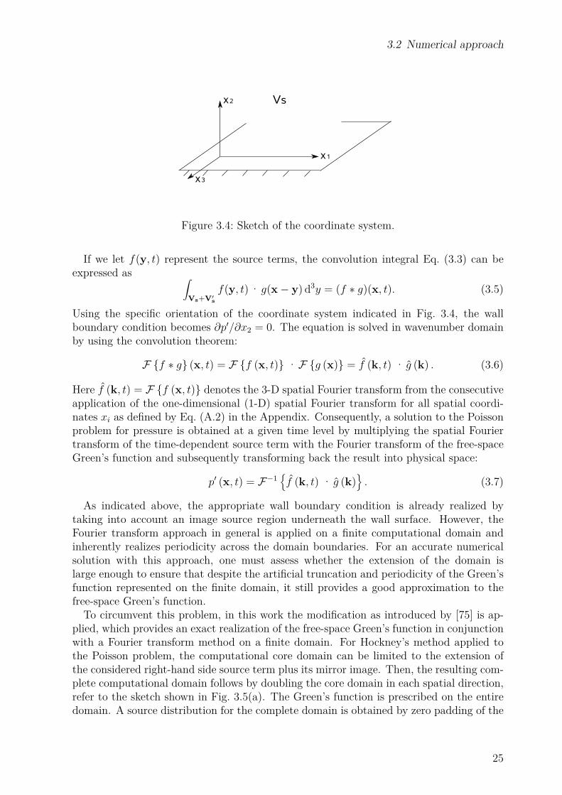
Here, u1 denotes the mean-flow velocity component in the x1-direction and u′i indicatesvelocity fluctuations; the x2-direction is the wall normal direction and the x3-direction isthe spanwise direction, refer to the coordinate system shown in Fig. 3.4; ρ0 is the meanair density and p′ is the fluctuating pressure. The source term on the right-hand side ofEq. (3.2) comprises two parts. The first part is the mean-shear turbulence interactionterm and the second part is the turbulence-turbulence interaction term. As addressed insection 2.1, the pressure fluctuations can be calculated from the convolution of the free-space Green’s function of the Poisson’s equation with the right-hand side source term,
p′(x, t) = −∫
Vs+V′sρ0
(2∂u1
∂x2
∂u′2(y, t)∂x1
+ ∂2
∂xi∂xj(u′iu′j − u′iu′j)(y, t)
)· g(x− y) dV (y),
(3.3)where Vs + V′s denotes the original source area plus the mirrored source area at the solidwall. The free-space Green’s function for a 3-D Poisson problem is given by
g(x− y) = − 14π|x− y|
. (3.4)
24
3.2 Numerical approach
x2
x3
x1
Vs
Figure 3.4: Sketch of the coordinate system.
If we let f(y, t) represent the source terms, the convolution integral Eq. (3.3) can beexpressed as ∫
Using the specific orientation of the coordinate system indicated in Fig. 3.4, the wallboundary condition becomes ∂p′/∂x2 = 0. The equation is solved in wavenumber domainby using the convolution theorem:
F {f ∗ g} (x, t) = F {f (x, t)} ·F {g (x)} = f (k, t) · g (k) . (3.6)
Here f (k, t) = F {f (x, t)} denotes the 3-D spatial Fourier transform from the consecutiveapplication of the one-dimensional (1-D) spatial Fourier transform for all spatial coordi-nates xi as defined by Eq. (A.2) in the Appendix. Consequently, a solution to the Poissonproblem for pressure is obtained at a given time level by multiplying the spatial Fouriertransform of the time-dependent source term with the Fourier transform of the free-spaceGreen’s function and subsequently transforming back the result into physical space:
p′ (x, t) = F−1{f (k, t) · g (k)
}. (3.7)
As indicated above, the appropriate wall boundary condition is already realized bytaking into account an image source region underneath the wall surface. However, theFourier transform approach in general is applied on a finite computational domain andinherently realizes periodicity across the domain boundaries. For an accurate numericalsolution with this approach, one must assess whether the extension of the domain islarge enough to ensure that despite the artificial truncation and periodicity of the Green’sfunction represented on the finite domain, it still provides a good approximation to thefree-space Green’s function.To circumvent this problem, in this work the modification as introduced by [75] is ap-
plied, which provides an exact realization of the free-space Green’s function in conjunctionwith a Fourier transform method on a finite domain. For Hockney’s method applied tothe Poisson problem, the computational core domain can be limited to the extension ofthe considered right-hand side source term plus its mirror image. Then, the resulting com-plete computational domain follows by doubling the core domain in each spatial direction,refer to the sketch shown in Fig. 3.5(a). The Green’s function is prescribed on the entiredomain. A source distribution for the complete domain is obtained by zero padding of the
25
3 Methods
x1+a1
x2
+a2
''wall''Vs
V's
=0
=0=0
periodic
-a1
-a2
(a)
x1+a1
x2
+a2
-a1
-a2
periodic
(b)
Figure 3.5: 2-D sketch to illustrate application of Hockney’s method with free field bound-ary condition; (a) source distribution with location of solid wall; (b) contourlines of free-space Green’s function Eq. (3.4).
source in the appended domains. Hence, the source function and the Green’s function forthe resolved domain become
f(x) ={f (x) , 0 ≤ xi ≤ ai; i ∈ {1...3}.0, else. (3.8)
g (x) = − 14π|x| , −ai ≤ xi ≤ ai; i ∈ {1...3}. (3.9)
To sketch the basic idea behind Hockney’s approach, it is convenient to consider theunderlying spatial convolution Eq. (3.5). If we seek for a solution to the Poisson problemjust in a core source domain of spatial extensions ai, the convolution integral includesproducts of the source term with the free-space Green’s function evaluated at a shiftedposition, which involve at maximum a shift in each direction given by ai. Hence, if aGreen’s function with periodic continuation is applied that is specified over twice the widthof the core source distribution, i.e. 2ai, Fig. 3.5(b), and no further source contributionis considered in the extended domain (zero padding), Fig 3.5(a), the convolution integralwill provide inside the core domain an exact solution to the Poisson problem based on thefree-space Green’s function.
3.2.2 Fast Random Particle-Mesh MethodAnisotropic synthetic turbulence
To calculate the fluctuating pressure an appropriate fluctuating velocity field within theturbulent boundary layer is needed. We use FRPM [87] to generate synthetic turbulentvelocity fluctuations to prescribe the right-hand side source term of Eq. (3.2). FRPM usesaveraged turbulence statistics to synthesize the turbulent velocity fluctuations. One- and
26
3.2 Numerical approach
two-point statistics are realized. The basic idea is to generate a fluctuating velocity vectorfrom the convolution of spatial white noise Ui with a spatial Gaussian filter kernel G,
u′i(x, t) = aik(x)∫Vsεklm
∂G (x− x′)∂xl
Um(x′, t)d3x′ (3.10)
where εklm denotes the Levi-Civita symbol (permutation tensor), x = (x1, x2, x3)T definesfield coordinates and x′ = (x′1, x′2, x′3)T defines white noise field coordinates. The Gaussianfilter is defined by the consecutive application of 1-D Gaussian filters based on separatelength scales li for each spatial direction,
The tensor aik provides the proper scaling so that the anisotropic Reynolds stress tensorcan be realized by the synthesized fluctuating velocity fields. Note, the summation rule isapplied over all equal indices.In this work a generic study is conducted on the influence of length scale anisotropy
on the resulting wall pressure spectrum. For this purpose, anisotropy in length scalesis considered using separate filter length scales li in the streamwise, wall-normal andspanwise directions, respectively. Furthermore, the streamwise length scale is increased bya stretching factor γ compared to the wall normal scale, l1 = γl2, whereas the length scalesin the wall-normal and spanwise directions are kept equal, l2 = l3. For the present study,the stretching factor is treated as a constant parameter throughout the computationaldomain. Note, in general three spatial length scales are associated with each Reynoldsstress component, yielding a third-rank tensor with 18 generally non-equal components.This anisotropic length scale information is not provided by RANS. In [92] an approach tostochastically model anisotropic length scales from RANS parameters for non-equilibriumturbulence has been proposed.In general, the length scale from RANS ls is considered as a scalar scale representing
all anisotropic scales [93] assuming the relationship ls = (l1l2l3)1/3, which yields l2 = l3 =lsγ−1/3.The scalar turbulent length scale ls is determined from the RANS solution via
ls = clCµ
√ktω, (3.13)
where kt = Rii/2 is the turbulent kinetic energy and ω is the specific rate of dissipation.The constant Cµ = 0.09 and cl is estimated to be 0.54 [94], so the prefactor cl/Cµ ' 6.0.The white noise field Ui is defined in a Lagrangian frame moving at local flow velocity U.
Altogether, the properties of white noise are defined in a fixed Eulerian frame by
where the bracket means an ensemble average, δij is the Kronecker symbol and δ(r−Uτ)describes frozen turbulence moving with the flow velocity U. Additional temporal turbu-lence decay can be modeled by a Langevin equation, which introduces the de-correlation in
27
3 Methods
the two-points statistics [87]. In the Eulerian frame a modification of the cross-correlationis given by
In this expression exp(−|τ |/τs) describes the turbulence decay, i.e. the field is spatiallywhite and correlated in time with time scale τs. The local time scale can be determinedfrom RANS solutions by
τs = cτls√kt, (3.17)
where the prefactor cτ needs to be determined. [95] modeled the time scale in a k−ε modeland determined the prefactor empirically by fitting experimental results of jet flows, whichresulted in cτ ' 0.91. In this work, a constant cτ = 1.2 is applied which is based on aconsistent result of the streamwise coherence of the wall pressure fluctuations comparedto the experimental results. The additional effect of the temporal turbulence decay forturbulence velocity fluctuation spectra is discussed in Appendix A.
Scaling tensor
For a stationary turbulent problem, straightforward manipulation of expression Eq. (3.10)yields the Reynolds stresses expressed in terms of the scaling tensor,
Rij(x) =⟨u′i(x, t)u′j(x, t)
⟩= aik(x)ajn(x)
∫Vsεklmεnop
∂G (x− x′)∂xl
∂G (x− x′′)∂xo
〈Um(x′, t)Up(x′′, t)〉 d3x′d3x′′ (3.18)
Based on Eq. (3.16) with τ = 0 and r = 0, the integration over the delta function relatedto x′′ can be carried out. Using the definition
Iij(x) :=∫Vs
∂G (x− x′)∂xi
∂G (x− x′)∂xj
d3x′, (3.19)
the Reynolds stresses eventually read (dependence on spatial coordinate not explicitlyshown)
Rij = aikajnεmlkεmonIlo. (3.20)Furthermore, using the identity εmlkεmon = δloδkn − δlnδko, it follows
Rij = aikajlSkl, (3.21)
where Skl = δklImm − Ilk defines a symmetric diagonal matrix, since Ilk = 0 for l 6= k asa result of its definition Eq. (3.19) with filter function Eq. (3.11). Let skm = c(k)δkm (thebrackets indicate omission of the summation rule) denote the diagonal matrix that followsby taking the square root of the diagonal elements of Skl = c(k)c(l)δkl (i.e. Skl = skmslm)and let rij denote the Cholesky decomposition of the Reynolds stress tensor, i.e. Rij =rimrjm, then the scaling tensor needed to evaluate Eq. (3.10) is defined by rim = aikskm,respectively,
aik = rik/c(k). (3.22)From the previous discussion it follows that the scaling explicitly is defined by c(k) =√Ill − Ik(k).
28
3.2 Numerical approach
Using the definition of the integral Eq. (3.19) together with the length scale defini-tions from the beginning of this section and applying the definition of the Gaussian filter,Eq. (3.11), the scaling parameters c(k) can be explicitly evaluated, yielding
c(1) =√πlsγ
1/3, c(2) =√πls2
√1 + γ2
γ2/3 , c(3) =√πls2
√1 + γ2
γ2/3 . (3.23)
Next, the Cholesky decomposition of the in general anisotropic Reynolds stress tensorRij from RANS with Reynolds stress model is deduced from
(rij) =
√R11 0 0
R21/r11
√R22 − r2
21 0R31/r11 (R32 − r21r31)/r22
√R33 − r2
31 − r232
, (3.24)
which can be solved starting with the first row and using successively for the evaluationof the consecutive rows already computed components of rij.According to this procedure, the tensor Skl can be Cholesky decomposed into the matrix
skm and the final scaling matrix follows by multiplying rim with the inverse of skm, aik =rims
−1km. The properties as defined by Eq. (3.19) guarantee that Skl is diagonal and can be
used to derive the scaling c(k) by taking the square root and the inverse of the diagonalelements, which essentially represents the Cholesky decomposition of Skl and leads toscaling equation (3.22).Eventually, the final anisotropic simulation is conducted by using the such determined
scaling matrix aik.
Isotropic turbulence
For isotropic turbulence the following relationships hold: aik(x) → a(x)δik, γ = 1 (i.e.l1 = l2 = l3 = ls), R11 = R22 = R33 = 2/3kt, and Rij = 0 for i 6= j. Consequently, fromEq. (3.22) the scalar scaling function for isotropic turbulence infers as
a (x) =
√√√√ 23π
kt (x)ls (x) . (3.25)
Furthermore, for homogeneous isotropic turbulence a = const. and integral Eq. (3.10)can be rewritten as
u′ = ∇× φφφ, (3.26)with φφφ = (φ1, φ2, φ3)T and
φi :=∫Vsa GUid3x′. (3.27)
The two-point correlations of the velocity fluctuations realise the normalized correlationtensor of homogeneous isotropic turbulence Rij(r) for two points xi and xj with distancer = |xi − xj| and the expected relationship between streamwise and spanwise correlationfunctions f(r) and g(r), respectively [96],
Rij = (f(r)− g(r))rirjr2 + g(r)δij, (3.28)
g(r) = f(r) + r
2df(r)dr
. (3.29)
29
3 Methods
For a Gaussian filter kernel defined by Eq. (3.11), the resulting streamwise correlationfunction for homogeneous isotropic turbulence is also a Gaussian [97] defined by
f(r) = exp(−πr
2
4l2s
). (3.30)
Based on the specific scaling of the Gaussian filter function Eq. (3.11), which leads to thestreamwise correlation Eq. (3.30), the length scale used therein complies with the integrallength scale L derived from the streamwise function,
L :=∫ ∞
0f(r)dr = ls. (3.31)
The length scale related to the spanwise correlation function obeys∫ ∞0
g(r)dr = ls2 . (3.32)
Numerical realization
For the quadrature of the integral in Eq. (3.10) the computational domain is formallysplit into equal sized non-overlapping control volumes δVp of constant size, continuouslycovering the resolved source domain without holes. A random particle is assigned tothe center of each control volume xp. All resulting particles are moving with their localconvection velocity at the particle location. The control volumes are bounded by liquid-linesurfaces, i.e. the boundary surface is drifting with the flow and in incompressible flow thecontrol volume δVp is invariant over time. The extension of the procedure to compressibleflow was discussed in [87]. Random variables are attached to each particle. Their randomvariates at time level tn+1 formally are defined by the integral over the control volume ofthe stochastic fields at the current time level, i.e.,
rn+1ip :=
∫δVpUi(x′, tn+1)d3x′. (3.33)
The notion ’random variate’ is used here to indicate the specific value of a random variableat a specific time level, e.g. random variates rn+1
ip indicate the value of random variablesrip at time level n+ 1. Eventually, the convolution Eq. (3.10) is approximated at discretetime level n+ 1 by summation over all control volumes,
u′n+1i (x) '
∑p
aikεklm∂
∂xlG(x− xp) rn+1
mp . (3.34)
Numerically, only random variables rmp are realized and the stochastic field Ui serves onlyto facilitate the derivation of a discretized random process to generate the actual variatesof each random variable.The numerical procedure to realize the simulation steps as discussed before relies on
an additional block structured mesh that defines the domain where synthetic turbulenceis generated, hereafter denoted as ’FRPM domain’. In this work a Cartesian equidistantmesh is used. However, also general curvilinear meshes could be used. The mean flow aswell as the local amplitude scaling function of the fluctuations, Eq. (3.25), and the locallength and time scales, Eq. (3.13) and (3.17), respectively, are evaluated from the RANSsolution and interpolated onto the FRPM mesh.
30
3.2 Numerical approach
For frozen turbulence, the random value carried by each particle is constant over time.Hence, its value is generated when a random particle is entering the computational do-main and kept constant while the particle is convected through the computational domain.When a random particle is leaving the computational domain it is reseeded with an up-dated random value at the upstream boundary so that the number of particles remainsinvariant and the mean particle density is conserved.For decaying turbulence a discretized Langevin equation is solved for each random
variate, refer to Ref. [87], whose discretized form reads [98]
rn+1ip =
(1− ∆t
τs
)rnip +
(2δVp ∆t
τs
)1/2
σnip, (3.35)
where σnip are mutually uncorrelated standardized Gaussian random variates, which areindependent of themselves at different times (
⟨σnip⟩
= 0,⟨σnipσ
mjq
⟩= δijδpqδnm), and which
are independent of rmip at past times (e.g.,⟨σnipr
mjq
⟩= 0 for tm ≤ tn. The time increment
between time levels tn+1 and tn is given by ∆t < τs. Furthermore, δVp indicates the controlvolume associated with each particle according to Eq. (3.33).For frozen turbulence (τs →∞), from the previous procedure it follows that rn+1
ip = rnip,i.e. the random variate is invariant over time. For frozen turbulence, the initial varianceof the random variate associated with each particle scales with δVp, i.e. the inverse localparticle density.Mean flow and other quantities needed at a specific particle position are obtained similar
to particle-in-cell (PIC) methods by trilinear mapping of the mean-flow information storedon the FRPM patch mesh from the corners of a specific hosting cell to the actual particleposition inside the cell.The complete algorithm to generate a fluctuating velocity field at time level n + 1 can
be summarized as follows:• based on the mean-flow velocity at the particle position, move the particles from old
position at time level n to the new one at time level n+ 1,
• realize with Eq. (3.35) new variates of all random variables attached to each particle,
• distribute random variates via discretized convolution Eq. (3.34) onto the sourcedomain,
• evaluate the right-hand side source term of the Poisson’s equation (3.2) and solve itvia Hockney’s method to predict the wall pressure at time level n+ 1.
The discretized convolution consists of a projection step, where the random variates aremapped from the actual particle position to the surrounding hosting cell nodes and thespatial filter steps are pursued sequentially on the FRPM mesh along each coordinatedirection using direction-dependent filter length scales li.In order to avoid a particle convecting on further away than into a cell attached to
the actual hosting cell, the maximum time step is limited by a Courant–Friedrichs–Lewy(CFL)–like condition based on the mesh spacing and the local mean-flow convection ve-locity.A discussion of the methods applied for the seeding of particles at inflow boundaries (and
removal at outflow boundaries) and the efficient realization of the discrete convolution viarecursive Gaussian filters can be found in Refs. [87] and [99].
31
4 Experimental results
In this chapter, the experimental results for the zero and non-zero pressure gradient bound-ary layer configurations are shown and discussed. Firstly, the mean flow characteristicsare obtained and summarized in section 4.1. The analysis of the measured one-point wallpressure spectra and their two-point features, namely the cross-spectra and the convectivevelocities, are discussed in section 4.2 and section 4.3.
4.1 Mean flow characteristicsThe mean velocity profiles for the zero pressure gradient (ZPG) cases were measuredat x = 1210 mm. The measurement position is about 60δ (boundary layer thicknessat the measurement location) distance downstream from the leading edge of the plateand is the location of the most downstream Kulite sensors. Five test velocities between20 m/s < U0 < 59 m/s were selected for ZPG flow measurements. Spanwise measurementsconfirmed an approximate 500-mm extent of uniform 2-D flow conditions at x = 1210 mm,refer to Figs. C.1-C.2 in Appendix C. ZPG conditions in the current study effectivelycorrespond to weak adverse pressure gradient (APG) conditions, i. e. to dCp/dx ≤ 0.1 m−1
between 930 mm ≤ x ≤ 1220 mm (refer also to Fig. 4.2).Fig. 4.1 shows the measured ZPG mean velocity profiles for all test velocities. The mean
velocities for locations y < 1.5 mm are estimated using Spalding’s equation [100],
y+ = u+ + e−κB[eκu
+ − 1− κu+ − (κu+)2
2 − (κu+)3
6
], (4.1)
where u+ = u/uτ and y+ = yuτ/ν. The friction velocity uτ is obtained by fitting themeasurement data to the log-law region. The present estimate applies constant κ = 0.41and B = 5.0 [101]. Spalding’s formula comprises all boundary layer regions in one singleexpression and provides an excellent fit from the sublayer to the log-law region [85].When normalized with the local free-stream velocity U0 and the boundary layer thick-
ness δ, Fig. 4.1(a), the profiles for U0 ≥ 39.2 m/s exhibit identical shapes, whereas thelower Reynolds number cases (20.3 m/s and 30.2 m/s) slightly deviate. The relevant char-acteristic parameters for the ZPG boundary layers are listed in Table 4.1. Accordingly,the observed scatter of the normalized velocity profiles for varying test speeds is well rep-resented by the shape factor H, where H = 1.42 for 20.3 m/s and H = 1.41 for 30.2 m/sare a little larger than H = 1.37–1.38 for the higher velocities. Following Clauser [77], His a function of Rex for equilibrium boundary layers, e.g. for 106 < Rex < 107 ZPG valuesof H are expected to vary between 1.26–1.35. Nikuradse [102] measured the boundarylayer for pipe flow in a range of 1.7 · 106 ≤ Rex ≤ 1.8 · 107. He found a universal meanvelocity distribution which is independent of Rex within the measurement range and de-rived constant H = 1.3. In a more recent study from Chauhan et al. [103], they collectedan extensive experimental dataset and established a relationship between the shape factorH and the boundary layer based Reynolds number. In the range of 3500 < Reθ < 8700,
33
4 Experimental results
0.0 0.2 0.4 0.6 0.8 1.0
y/δ
0.0
0.2
0.4
0.6
0.8
1.0
u/U
0
20.3 m/s
30.2 m/s
39.2 m/s
49.1 m/s
58.7 m/s
(a)
100 101 102 103
y+
0
5
10
15
20
25
30
u+
20.3 m/s
30.2 m/s
39.2 m/s
49.1 m/s
58.7 m/s
(b)
Figure 4.1: Boundary layer mean velocity profiles for ZPG at velocities between 20 m/s <U0 < 59 m/s, x = 1210 mm.
Table 4.1: Boundary layer parameters for ZPG.U0 δ δ∗ θ H uτ Rex = Reτ = Reθ = dp/dx βδ∗
the shape factor is between 1.35–1.4. Overall, the obtained values of H from the currentmeasurement are slightly larger than the results from the literature, which is probably dueto the present little APG in the plate rear region.APG boundary layers were realized by means of the NACA 0012 airfoil at geometric
angles of attack (AOAs) of -6◦, -10◦ and -14◦, and favorable pressure gradient (FPG)boundary layers at 12◦ and 14◦. The following analysis of the data under pressure gra-dients is limited to the free-stream velocity of 30.2 m/s. Fig. 4.2 shows the measureddistributions of the pressure coefficient Cp between 930 mm ≤ x ≤ 1220 mm. Due to thepresence of the airfoil, the shear layer from the nozzle and the flow field underneath theairfoil can be impacted, e.g. an acceleration of the flow underneath the airfoil will cause alocally lower pressure, which can suck the shear layer towards the midline. The measuredCp distributions in the spanwise direction confirmed a nearly 2-D flow condition in themeasurement region, refer to C.3 in Appendix C.Velocity profiles were measured at two positions x = 1128 mm and x = 1210 mm, where
the most upstream and downstream Kulite sensors were located. Fig. 4.3 shows the meanvelocity profiles for ZPG, APG and FPG boundary layers at x = 1210 mm. The measuredtrends show good agreement with the experimental results from the literature [85]. TheFPG boundary layer shows a larger velocity increase in the inner layer, when comparedto the ZPG case. Contrarily, the APG boundary layer exhibits a steeper velocity increase
34
4.1 Mean flow characteristics
900 950 1000 1050 1100 1150 1200 1250x [mm]
1.0
0.8
0.6
0.4
0.2
0.0
0.2
0.4
Cp
ZPGAPG 6 ◦
APG 10 ◦
APG 14 ◦
FPG 12 ◦
FPG 14 ◦
Figure 4.2: Cp distributions in the streamwise direction between 930 mm ≤ x ≤ 1220 mm.
0.0 0.2 0.4 0.6 0.8 1.0
y/δ
0.0
0.2
0.4
0.6
0.8
1.0
u/U
0
ZPGAPG 6 ◦
APG 10 ◦
APG 14 ◦
FPG 12 ◦
FPG 14 ◦
(a)
100 101 102 103
y+
0
10
20
30
40
50
60
u+
ZPGAPG 6 ◦
APG 10 ◦
APG 14 ◦
FPG 12 ◦
FPG 14 ◦
(b)
Figure 4.3: Mean velocity profiles for ZPG and non-ZPG at x = 1210 mm for the free-stream velocity of 30.2 m/s.
in the outer layer. For a very strong APG boundary layer, e. g. the APG -14◦ case, aninflection point occurs at the transition region between the inner and outer layers, i. e. atabout 0.1–0.2 δ. If we plot the profiles in log-law representation, all profiles collapse to asingle curve in the inner layer, as shown in Fig. 4.3(b).Table 4.2 summarizes the relevant APG and FPG boundary layer parameters for the
two selected velocity measurement positions at the rear part of the plate. Note that for theAPG cases the local pressure gradients dp/dx and the NACA 0012 geometrical AOAs showinconsistent trends, whereas consistent trends are limited to the more upstream locations(refer to Fig. 4.2).From Fig. 4.3 (x = 1210 mm) one could conclude, that both the shape factor H and
Clauser’s equilibrium parameter βδ∗ can be used to correctly represent the described ZPGand APG effects on the mean velocity profile shape. However, compared to H, βδ∗ isdirectly impacted by the local pressure gradient, and a stronger local dp/dx does not
35
4 Experimental results
Table 4.2: Boundary layer parameters for APG and FPG at the free-stream velocity of30.2 m/s.
necessarily indicate the upstream boundary layer developmental history of a much strongerinitial APG or FPG.For example, if we compare βδ∗ and H as derived at the two different measurement
positions for the APG -10◦ and APG -14◦ cases, the values show reverse trends: whenmoving downstream from x = 1128 mm to x = 1210 mm, the parameter H increases,whereas βδ∗ decreases. In Fig 4.4(a) it is documented, that the measured velocity profilescannot be sorted in the correct order based on βδ∗ . On the contrary, H perfectly capturesthe developed trends. The measured profile shapes indicate that the velocity profiles atx = 1210 mm are still significantly affected by the strong initial APG conditions. A plotof the corresponding defect profiles is shown in Fig 4.4(b). An equilibrium boundary layerpresents a larger velocity gradient in the outer layer for a greater value of βδ∗ [77, 83,104]. The measured APG boundary layers in the current study show reversed trends,indicating that Clauser’s equilibrium parameter βδ∗ is not suited to define the shape of thevelocity profiles for arbitrary non-equilibrium boundary layers, especially for cases withfast pressure gradient changes.
4.2 One-point spectraFig. 4.5(a) shows the wall pressure one-point power spectral densities (psd) for ZPG bound-ary layers at x = 1210 mm. Spectral levels in this thesis are referenced to a 20 µPa refer-ence pressure. The measured one-point spectra are analyzed with a window length of 4096samples. The sampling rate is 100 kHz, which results in a resolution of about 24 Hz. Thespectra show a good overall agreement with predictions using Goody’s [36] model. Es-pecially for the higher velocities the measured spectra are contaminated by setup-relateddisturbances at both low and high frequencies; the spectral increase at frequencies belowabout 230 Hz for U0 =58.7 m/s is due to the impact of the open-jet free shear layer (fea-turing a much higher velocity scaling exponent than the turbulent boundary layer wall
36
4.2 One-point spectra
0.0 0.2 0.4 0.6 0.8 1.0y/δ
0.0
0.2
0.4
0.6
0.8
1.0
u/U
0
ZPGAPG 10 ◦ , x=1128 mm, H=1.63, βδ ∗ =6.8
APG 10 ◦ , x=1210 mm, H=1.75, βδ ∗ =6.0
APG 14 ◦ , x=1128 mm, H=1.91, βδ ∗ =16.2
APG 14 ◦ , x=1210 mm, H=2.12, βδ ∗ =12.5
(a)
0.0 0.2 0.4 0.6 0.8 1.0y/δ
0
10
20
30
40
50
(U0−u)/uτ
ZPGAPG 10 ◦ , x=1128 mm, H=1.63, βδ ∗ =6.8
APG 10 ◦ , x=1210 mm, H=1.75, βδ ∗ =6.0
APG 14 ◦ , x=1128 mm, H=1.91, βδ ∗ =16.2
APG 14 ◦ , x=1210 mm, H=2.12, βδ ∗ =12.5
(b)
Figure 4.4: Mean velocity profiles for ZPG and APG -10◦ & -14◦.
102 103 104
frequency [Hz]
40
50
60
70
80
90
psd
[dB
]
20.3 m/s
30.2 m/s
39.2 m/s
49.1 m/s
58.7 m/s
(a)
100 101 102
ωδ/Ue
40
30
20
10
0
10
10lo
g[Φ
(ω)U
e/τ
2 wδ]
20.3 m/s
30.2 m/s
39.2 m/s
49.1 m/s
58.7 m/s
(b)
Figure 4.5: (a) One-point spectra for different velocities compared with predictions accord-ing to Goody [36], x = 1210 mm; (-), measured spectra; (- -), Goody spectra;(b) spectra scaled by τw as pressure scale and δ/Ue as time scale.
pressures) while the resonance frequency for the Kulite-pinhole-arrangement was locatedat about 30 kHz. However, an impact of the resonance is found down to 7 kHz for 49.1 m/sand 58.7 m/s. Spectral levels below 48 dB are buried by the electrical noise of the appliedKulite sensor.When scaled based on mixed parameters, as Goody proposes, the normalized spectra
collapse to a single curve at mid Strouhal numbers ωδ/Ue with a slope of ω−0.7, seeFig. 4.5(b). The boundary layer edge velocity Ues is herein set to Ue = 0.99U0. Thismid Strouhal number range is primarily attributed to the log-law region of the boundarylayer at a ZPG [50]. The similarity of the velocity profile might predominantly contributeto the collapse of the spectra at these medium frequencies. A Reynolds number effectat high frequencies is expressed as an elongated mid-frequency ω−0.7 range, which is wellidentified by Goody using the model parameter RT = Reτ
√Cf/2, where Cf is the skin
37
4 Experimental results
friction coefficient. Minor deviations are observed at the low Strouhal number range, wherethe measured spectra appear free of disturbances: the present measurements indicate adependence of the low-frequency slope and the maximum location on the Reynolds number,whereas Goody proposes identical spectral shapes in the low and medium Strouhal numberranges. Particularly, at U0 = 20.3 m/s the spectral increase is steeper at low Strouhalnumbers and the maximum is located at a higher Strouhal number compared to the spectrafor the other velocities. Similar observations were made by Farabee & Casarella [8] andLeclercq & Bohineust [9]. Panton & Linebarger [49] and the author (refer to Fig. 6.6)calculated the contributions from different decks of the boundary layer and found thatthe spectra at low frequencies are composed of contributions from both the inner andouter layers. Based on this argument it is reasonable to conclude that an elongated mid-frequency range might change the shape of the spectra also at low frequencies. Note that,the slightly changed velocity profile shape at smaller U0, also discussed as a Reynoldsnumber effect, is in line with the observation of a changed shape of the corresponding wallpressure spectrum.Figs. 4.6(a–e) show the wall pressure one-point spectra for APG and FPG boundary
layers at the free-stream velocity of 30.2 m/s. The corresponding ZPG spectrum is plottedas reference. The spectral form in dependence of the initial pressure gradient conditionsis well illustrated. Compared to the ZPG spectra the APG spectra feature an increasein maximum level and a steeper slope at medium frequencies with consistent trends asobserved for the corresponding velocity profiles. For a given initial APG configuration,when moving downstream, the spectra shift towards lower frequencies and the slope atmedium frequencies becomes successively steeper. For the FPG configurations the spectralslope at higher frequencies > 1 kHz is successively flattened, when moving downstream.The higher spectral level at lower frequencies < 1 kHz, especially even larger than theZPG case, is unexpected. A flattened spectral slope at lower frequencies was measuredby Salze et al. [44] and Suryadi & Herr [45]. This hump measured at lower frequenciesmay be caused by some unexpected effects due to the present NACA airfoil. A stronginterference occurs at low frequencies for the FPG 14◦ case, which is probably caused bythe fully separated flow on the suction side of the NACA airfoil.Fig. 4.6(f) shows the scaled spectra for ZPG, APG and FPG boundary layers at x =
1210 mm using the same scaling parameters as for the ZPG spectra. Unlike the goodcollapse of the ZPG spectra, normalized levels diverge by up to 20 dB. Again, the evolutionof the mid-frequency slope from a FPG boundary layer to an APG boundary layer is wellillustrated. Note that the roll-off slope of ω−5 at high frequencies appears to be unaffectedfor both APG and FPG spectra. A very good collapse for the ZPG and APG spectralmaxima is found by scaling with uτ/Q2θ and ωθ/U0, see Fig. 4.7(a). All the measured APGspectra at x = 1128 mm and 1210 mm including the free-stream velocities of 20.3 m/s and39.1 m/s are scaled using these parameters and a good collapse of the spectral maxima isshown in Fig. 4.7(b). It is worth to note that a comparably good collapse is also foundfor spectral scaling based on uτ/Q2δ or U0/Q
2δ∗, refer to Fig. C.4 in Appendix C. All thescalings are based on the dynamic pressure Q. It seems to be more reasonable to scale theAPG spectra using the outer pressure scale Q instead of τw. However, different from thecommonly used outer parameters U0/Q
2δ, a mixed representation for the involved timescales is used to consider the effect of an APG boundary layer. It is also worth to mentionthat if the FPG spectral level does not increase at lower frequencies < 1 kHz, the spectralpeak for the FPG cases can also collapse with the ZPG and APG spectra by using a scaling
38
4.2 One-point spectra
102 103 104
frequency [Hz]
50
55
60
65
70
75
80
85
90
psd
[dB
]
x= 1128 mm
x= 1168 mm
x= 1195 mm
x= 1210 mm
ZPG
(a)
102 103 104
frequency [Hz]
50
55
60
65
70
75
80
85
90
psd
[dB
]
x= 1128 mm
x= 1168 mm
x= 1195 mm
x= 1210 mm
ZPG
(b)
102 103 104
frequency [Hz]
50
55
60
65
70
75
80
85
90
psd
[dB
]
x= 1128 mm
x= 1168 mm
x= 1195 mm
x= 1210 mm
ZPG
(c)
102 103 104
frequency [Hz]
50
55
60
65
70
75
80
85
90psd
[dB
]
x= 1128 mm
x= 1168 mm
x= 1195 mm
x= 1210 mm
ZPG
(d)
102 103 104
frequency [Hz]
50
55
60
65
70
75
80
85
90
psd
[dB
]
x= 1128 mm
x= 1168 mm
x= 1195 mm
x= 1210 mm
ZPG
(e)
100 101
ωδ/Ue
20
15
10
5
0
5
10
15
20
10lo
g[Φ
(ω)U
e/τ
2 wδ]
APG 14 ◦
APG 10 ◦
APG 6 ◦
ZPGFPG 12 ◦
FPG 14 ◦
(f)
Figure 4.6: One-point spectra for the free-stream velocity of 30.2 m/s; (a) APG -14◦; (b)APG -10◦; (c) APG -6◦; (d) FPG 12◦; (e) FPG 14◦; (f) spectra at x = 1210 mm,scaled by τw as pressure scale and δ/Ue as time scale.
39
4 Experimental results
10-1 100 101
ωθ/U0
90
85
80
75
70
65
60
55
50
10lo
g(Φ
(ω)u
τ/Q
2θ)
ZPG
APG 6 ◦
APG 10 ◦
APG 14 ◦
(a)
10-1 100 101
ωθ/U0
90
85
80
75
70
65
60
55
50
10lo
g(Φ
(ω)u
τ/Q
2θ)
(b)
Figure 4.7: Spectra scaled by uτ/Q2θ and θ/U0; (a) spectra for ZPG and APG at x =
1210 mm for the free-stream velocity of 30.2 m/s; (b) spectra for APG 6◦, 10◦and 14◦ at x = 1128 mm and x = 1210 mm for the free-stream velocities of20.3 m/s, 30.2 m/s and 39.2 m/s.
based on Q, refer to Fig. C.5 in Appendix C.
4.3 Cross-spectra and convective velocitiesFrom the two-point statistics obtained from the sensors located in different streamwise andspanwise positions, the spatial and temporal properties of the wall fluctuating pressurefield can be studied. Corcos [51] used exponential functions (addressed in section 2.2)to characterize the streamwise and spanwise coherences of the pressure field by takingadvantage of the similarity of the coherence decay, expressed as
where α and β are empirical constants which are in charge of prescribing the turbulencedecay in the streamwise and spanwise directions, respectively. The value of α depends onthe Reynolds number. Generally, a smaller value relates to a larger Reynolds number. Inthe present measurement for ZPG boundary layers the obtained value of α decreases from0.15 to 0.125 as the Reynolds number Reτ increases from 1040 to 2499. A similar trendwas reported by Farabee & Casarella [8], with α = 0.145 for Reτ = 1169 and α = 0.125for Reτ = 2010. The obtained value of β shows no noticeable dependence on Reynoldsnumber, β = 0.72 for all measured velocities in ZPG boundary layers. The value of β isreported only in few experiments. Bull [6] obtained β = 0.715 in a ZPG boundary layer,which is consistent with the present results.In Eq. (4.2), Uc is the convective phase velocity of the wall fluctuating pressure field and
it is defined by Uc(r1, ω) = r1ω/θ(r1, ω), where θ(r1, ω) is the phase difference of Γ(r1, 0, ω).The phase velocity depends on the streamwise separations. To present the coherence witha separation of r1 in the streamwise direction, a phase velocity Uc(r1, ω) obtained at thesame streamwise separation is used. However, the application for the phase velocity Uc inthe spanwise direction is not explicit. Bull [6] used an averaged Uc(ω) obtained from the
40
4.3 Cross-spectra and convective velocities
streamwise direction. Brooks & Hodgson [82] applied a streamwise separation dependentUc(r1, ω), which used r1 = r3 to calculate the spanwise coherence at a separation of r3. Itis the authors’ understanding that a phase velocity Uc(r1 → 0, ω) which indicates the localphase velocity is more meaningful to apply. However, Uc(r1 → 0, ω) cannot be measured.In this work the phase velocity Uc(ω) obtained from the two closest sensors r1 = 2 mm atthe most downstream direction is used to represent the spanwise coherence.Figs. 4.8-4.9 show the streamwise and spanwise coherences at the free-stream velocity
of 30.2 m/s for ZPG, APG and FPG boundary layers, respectively. A window length of2048 samples is used to calculate the coherence. The streamwise coherence for APG andFPG boundary layers are only calculated from the sensors located between 1183 mm<x <1210 mm where very similar spectra are measured. This implies a similar boundarylayer condition within this range. The spanwise coherence was measured at x =1210 mm.The streamwise and spanwise coherence curves for the ZPG boundary layer collapse athigher frequencies and can be well fitted by the exponential functions with α = 0.14 andβ = 0.72, see Figs. 4.8(a)-4.9(a). The obtained exponential function for prescribing thestreamwise and spanwise coherences of the ZPG boundary layer is also plotted in theresults for APG and FPG boundary layers for comparison. It is worth to note that theconvection of the flow field results in an offset for samples in the streamwise direction andtherefore reduces the obtained streamwise coherence [25]. To reduce this effect, the timeshift between the different streamwise positions is calculated using the mean flow velocityUc(r1) and the time shift is applied to calculate the streamwise coherence.Figs. 4.8(b-d) show the streamwise coherence for APG boundary layers. It clearly illus-
trates that an APG boundary layer causes an increased coherence decay in the streamwisedirection. The larger the APG, the stronger the decay. This implies the APG enhancesthe turbulence decay rate during the eddies downstream convection in the boundary layer.Similar observations were reported by Schloemer [38], Brooks & Hodgson [82] and Catlettet al. [48]. Note that, even for the strongest initial APG (APG -14◦ case) the streamwisecoherence shows the similarity scaling behavior, although the trend can be not necessarilycharacterized using a single exponential function. The larger frequencies share a strongerdecay rate (a larger constant for the exponential function), this feature may be related tothe different phase velocity trends from low frequencies to higher frequencies between ZPGand APG boundary layers, see Fig. 4.10. The phase velocity of the APG boundary layersshows that the velocity at higher frequencies is much smaller than at lower frequenciescompared to the ZPG boundary layer, and a smaller velocity means a longer travel timeover a constant distance which could cause a larger decay. Figs. 4.8(e-f) show a slightlyincreased streamwise coherence in FPG boundary layers.Figs. 4.9(b-f) show a smaller decay rate for the spanwise coherence in an APG boundary
layer and a larger decay rate in a FPG boundary layer. Note that the coherence curvescollapse in FPG boundary layers but not any more in strong APG boundary layers, e.g.the APG -10◦ and APG -14◦ cases.Fig. 4.10 shows the convective phase velocities at the free-stream velocity of 30.2 m/s
for ZPG, APG and FPG boundary layers. A larger velocity is measured at a largerstreamwise distance for all the configurations. This is because the smaller eddies closeto the wall moving with a slower velocity decay faster as convecting downstream, thusat the larger distance the velocity is rather attributed to the larger eddies moving with ahigher velocity. It is found that the obtained velocity decreases for an APG boundary layercompared to the ZPG boundary layer while it increases for a FPG boundary layer. This
41
4 Experimental results
0 2 4 6 8 10 12 14ωr1/Uc (r1 ,ω)
0.0
0.2
0.4
0.6
0.8
1.0
Γ(r
1,ω
)
r1/δ∗ =0.6
r1/δ∗ =1.7
r1/δ∗ =4.3
r1/δ∗ =7.7
r1/δ∗ =12.0
r1/δ∗ =17.1
r1/δ∗ =23.4
exp(−0.14ωr1/Uc )
(a)
0 2 4 6 8 10 12 14ωr1/Uc (r1 ,ω)
0.0
0.2
0.4
0.6
0.8
1.0
Γ(r
1,ω
)
r1/δ∗ =0.4
r1/δ∗ =0.7
r1/δ∗ =1.1
r1/δ∗ =1.6
r1/δ∗ =2.3
r1/δ∗ =2.7
r1/δ∗ =3.7
r1/δ∗ =4.5
r1/δ∗ =4.8
exp(−0.14ωr1/Uc )
(b)
0 2 4 6 8 10 12 14ωr1/Uc (r1 ,ω)
0.0
0.2
0.4
0.6
0.8
1.0
Γ(r
1,ω
)
r1/δ∗ =0.3
r1/δ∗ =0.5
r1/δ∗ =0.8
r1/δ∗ =1.2
r1/δ∗ =1.7
r1/δ∗ =2.0
r1/δ∗ =2.7
r1/δ∗ =3.3
r1/δ∗ =3.5
exp(−0.14ωr1/Uc )
(c)
0 2 4 6 8 10 12 14ωr1/Uc (r1 ,ω)
0.0
0.2
0.4
0.6
0.8
1.0
Γ(r
1,ω
)
r1/δ∗ =0.2
r1/δ∗ =0.3
r1/δ∗ =0.5
r1/δ∗ =0.7
r1/δ∗ =1.1
r1/δ∗ =1.2
r1/δ∗ =1.7
r1/δ∗ =2.1
r1/δ∗ =2.2
exp(−0.14ωr1/Uc )
(d)
0 2 4 6 8 10 12 14ωr1/Uc (r1 ,ω)
0.0
0.2
0.4
0.6
0.8
1.0
Γ(r
1,ω
)
r1/δ∗ =1.0
r1/δ∗ =2.0
r1/δ∗ =3.1
r1/δ∗ =4.6
r1/δ∗ =6.6
r1/δ∗ =7.7
r1/δ∗ =10.7
r1/δ∗ =12.8
r1/δ∗ =13.8
exp(−0.14ωr1/Uc )
(e)
0 2 4 6 8 10 12 14ωr1/Uc (r1 ,ω)
0.0
0.2
0.4
0.6
0.8
1.0
Γ(r
1,ω
)
r1/δ∗ =1.6
r1/δ∗ =3.1
r1/δ∗ =4.7
r1/δ∗ =7.0
r1/δ∗ =10.2
r1/δ∗ =11.7
r1/δ∗ =16.4
r1/δ∗ =19.5
r1/δ∗ =21.1
exp(−0.14ωr1/Uc )
(f)
Figure 4.8: Streamwise coherence as a function of ωr1/Uc(r1, ω) at the free-stream velocityof 30.2 m/s; (a) ZPG; (b) APG -6◦; (c) APG -10◦; (d) APG -14◦; (e) FPG 12◦;(f) FPG 14◦.
42
4.3 Cross-spectra and convective velocities
0 1 2 3 4 5ωr3/Uc (ω)
0.0
0.2
0.4
0.6
0.8
1.0
Γ(r
3,ω
)
r1/δ∗ =0.6
r1/δ∗ =1.1
r1/δ∗ =1.7
r1/δ∗ =3.7
exp(−0.72ωr3/Uc )
(a)
0 1 2 3 4 5ωr3/Uc (ω)
0.0
0.2
0.4
0.6
0.8
1.0
Γ(r
3,ω
)
r1/δ∗ =0.4
r1/δ∗ =0.7
r1/δ∗ =1.1
r1/δ∗ =2.3
exp(−0.72ωr3/Uc )
(b)
0 1 2 3 4 5ωr3/Uc (ω)
0.0
0.2
0.4
0.6
0.8
1.0
Γ(r
3,ω
)
r1/δ∗ =0.3
r1/δ∗ =0.5
r1/δ∗ =0.8
r1/δ∗ =1.7
exp(−0.72ωr3/Uc )
(c)
0 1 2 3 4 5ωr3/Uc (ω)
0.0
0.2
0.4
0.6
0.8
1.0Γ(r
3,ω
)r1/δ
∗ =0.2
r1/δ∗ =0.3
r1/δ∗ =0.5
r1/δ∗ =1.1
exp(−0.72ωr3/Uc )
(d)
0 1 2 3 4 5ωr3/Uc (ω)
0.0
0.2
0.4
0.6
0.8
1.0
Γ(r
3,ω
)
r1/δ∗ =1.0
r1/δ∗ =2.0
r1/δ∗ =3.1
r1/δ∗ =6.6
exp(−0.72ωr3/Uc )
(e)
0 1 2 3 4 5ωr3/Uc (ω)
0.0
0.2
0.4
0.6
0.8
1.0
Γ(r
3,ω
)
r1/δ∗ =1.6
r1/δ∗ =3.1
r1/δ∗ =4.7
r1/δ∗ =10.2
exp(−0.72ωr3/Uc )
(f)
Figure 4.9: Spanwise coherence as a function of ωr3/Uc(ω) at the free-stream velocity of30.2 m/s; (a) ZPG; (b) APG -6◦; (c) APG -10◦; (d) APG -14◦; (e) FPG 12◦;(f) FPG 14◦.
43
4 Experimental results
0 5 10 15 20
ωδ/U0
0.2
0.3
0.4
0.5
0.6
0.7
0.8
0.9
Uc(r
1,ω
)/U
0
r1/δ∗ = 0.6
r1/δ∗ = 1.7
r1/δ∗ = 4.3
r1/δ∗ = 7.7
r1/δ∗ = 12.0
r1/δ∗ = 17.1
r1/δ∗ = 23.4
(a)
0 5 10 15 20
ωδ/U0
0.2
0.3
0.4
0.5
0.6
0.7
0.8
0.9
Uc(r
1,ω
)/U
0
r1/δ∗ = 0.4
r1/δ∗ = 1.1
r1/δ∗ = 2.7
r1/δ∗ = 4.8
r1/δ∗ = 7.5
r1/δ∗ = 10.7
(b)
0 5 10 15 20
ωδ/U0
0.2
0.3
0.4
0.5
0.6
0.7
0.8
0.9
Uc(r
1,ω
)/U
0
r1/δ∗ = 0.3
r1/δ∗ = 0.8
r1/δ∗ = 2.0
r1/δ∗ = 3.5
r1/δ∗ = 5.5
r1/δ∗ = 7.8
(c)
0 5 10 15 20
ωδ/U0
0.2
0.3
0.4
0.5
0.6
0.7
0.8
0.9
Uc(r
1,ω
)/U
0
r1/δ∗ = 0.2
r1/δ∗ = 0.5
r1/δ∗ = 1.2
r1/δ∗ = 2.2
r1/δ∗ = 3.5
r1/δ∗ = 5.0
(d)
0 5 10 15 20
ωδ/U0
0.2
0.3
0.4
0.5
0.6
0.7
0.8
0.9
Uc(r
1,ω
)/U
0
r1/δ∗ = 1.0
r1/δ∗ = 3.1
r1/δ∗ = 7.7
r1/δ∗ = 13.8
r1/δ∗ = 21.4
r1/δ∗ = 30.6
(e)
0 5 10 15 20
ωδ/U0
0.2
0.3
0.4
0.5
0.6
0.7
0.8
0.9
Uc(r
1,ω
)/U
0
r1/δ∗ = 1.6
r1/δ∗ = 4.7
r1/δ∗ = 11.7
r1/δ∗ = 21.1
r1/δ∗ = 32.8
(f)
Figure 4.10: Phase velocities as a function of ωδ/Uc(r1, ω); (a) ZPG; (b) APG -6◦; (c) APG-10◦; (d) APG -14◦; (e) FPG 12◦; (f) FPG 14◦.
44
4.3 Cross-spectra and convective velocities
0 5 10 15 20 25 30
r1/δ∗
0.3
0.4
0.5
0.6
0.7
0.8
0.9
Uc/U
0
ZPGAPG, 6 ◦
APG, 10 ◦
APG, 14 ◦
FPG, 12 ◦
FPG, 14 ◦
Figure 4.11: Mean convective velocity U c at the free-stream velocity of 30.2 m/s.
trend is primarily a result of the different mean velocity profile shapes for the boundarylayers. The important portion y < 0.5δ in the boundary layer for the wall pressurefluctuations owns a larger mean flow velocity u/U0 for the FPG boundary layer than theAPG boundary layer, see Fig. 4.3(a). The smallest mean flow velocity in this portion isfound in the APG -14◦ case with the smallest convective velocities.Another view on the convective features can be obtained from the mean convection veloc-
ity U c computed using the time shift τ of the maximum correlation for a fixed streamwiseseparation r1, U c(r1) = r1/τ(r1). The results for ZPG, APG and FPG boundary layers atthe free-stream velocity of 30.2 m/s are shown in Fig. 4.11. It shows the same trend asobtained from the phase velocity, namely a FPG boundary layer has a faster convectivevelocity while an APG boundary layer a slower one. The maximum mean convective ve-locity approaches 0.82U0 for the FPG boundary layer and < 0.7U0 for the strong APGboundary layer of 14◦. The maximum mean convective velocity implies the position ofthe ’longest lived’ eddies in the boundary layer, if we assume the obtained velocity originsfrom the region of the boundary layer where the eddies convect with the same velocity. Itis found that the position of the ’longest lived’ eddies moves far away from the wall froma FPG boundary layer to an APG boundary, see Fig. 4.3(a).
45
5 Formulation of an empirical model forone-point spectra
From the analysis of the one-point spectra in section 4.2, we found a good collapse of thespectral maxima by using the outer parameters to scale the spectra for zero and adversepressure gradients, refer to Fig. 4.7. A clear trend for the slope at medium frequencies anda nearly unchanged high-frequency roll-off slope were observed. From these observations,we are encouraged to develop an empirical spectral model for adverse pressure gradient(APG) wall pressure fluctuations based on a modification of the zero pressure gradient(ZPG) wall pressure spectrum.The measured data presented in this work are used to discuss the effect of the APG on
the spectral form. The Goody model is used as the basic form and the impact of each ofits parameters on the spectral form is discussed. A modification of the Goody model ismade to be able to predict the measured data for the APG cases. The detailed discussionand derivation of the modification is addressed in section 5.1.In section 5.2, datasets from five different experiments at four different test facilities,
covering a large range of Reynolds number 2.6 · 103 < Reθ < 1.9 · 104, are selected toinvestigate the proposed modification in section 5.1 and the published APG wall pressurespectral models. Predictions of the APG cases from the selected datasets also includingone ZPG test case are made and compared to the measured spectra. Features of eachpublished model and the proposed modification are discussed.Based on the comparison and discussion made in section 5.2, an improvement of the
proposed modification in section 5.1 is made in section 5.3. The final formulation of thenew empirical model for the APG wall pressure spectra (also capable to predict the ZPGspectra) is proposed. The prediction of the proposed new model shows good agreementwith the measured spectra.
5.1 Parametric analysis and modification approachTo some extent, the APG spectra have similar trends as the ZPG spectra, refer to Fig. 4.7.The spectra increase first at low frequencies, then drop at medium frequencies and roll offat high frequencies. Goody’s model can well represent these trends for ZPG spectra inthe three different ranges, especially at medium and high frequencies. From this point itis appropriate to take Goody’s model as the starting point. Goody’s model is expressedas
Φ(ω)Ueτ 2wδ
= a· (ωδ/Ue)b[(ωδ/Ue)c + d]e + [f · (ωδ/Ue)]g
, (5.1)
where the value of the parameters a–g was obtained by fitting the measurement data fromthe literature, a = 3, b = 2, c = 0.75, d = 0.5, e = 3.7, f = 1.1R−0.57
T and g = 7. Goodyused Ue/τ 2
wδ and ωδ/Ue as scaling parameters for the ZPG spectra. However, based on theprevious discussion in section 4.2 it is more appropriate to use uτ/Q2θ and ωθ/U0 as the
47
5 Formulation of an empirical model for one-point spectra
scaling parameters for the APG spectra. It is worth to mention that the chosen scalingparameters provide a better trend in fitting the maximum locations of the spectra thanthe other two proper scaling parameters mentioned before based on the measured data.Thus, Goody’s model is rewritten as
The parameters a–g in this equation control the shape of the dimensionless spectra. Theamplitude of the spectra is adjusted by the value of a. The slopes in different frequencyranges are driven by the combination of b, c, e and g. The parameter f determines theextension of the mid-frequency range. The maximum location is affected by the value ofd, the slope at low frequencies and the trend of the transition range between the increaseand decrease at low and medium frequencies.The first step of the modification is to represent the ZPG spectra which are supposed to
have a trend of ω−0.7 at medium frequencies and ω−5 at high frequencies. This trend canbe realized by means of the combination of the parameters, which follows b− c· e = −0.7and b − g = −5. Goody adopted b = 2 from the Chase-Howe [34] model, which impliesan ω2 increase at low frequencies. Panton & Linebarger [49] and Blake [50] calculatedthe spectra of the wall pressure fluctuations by solving a Poisson’s equation. The resultis derived by integration of the contributions throughout all decks of the boundary layer.Due to the term k2
1/k2 exp(−2ky) in the solution, where k1 is the wavenumber in the
streamwise direction, k2 = k21 + k2
3 and y is the wall-normal distance to the wall, anω2 increase at low frequencies is obtained. However, in the calculation the fluctuationdynamics is assumed as frozen turbulence. The spectra for both frozen turbulence andnon-frozen turbulence are calculated in section 6.1, refer to Fig. 6.6. The result showsthat the ω2 increase does not hold if non-frozen turbulence is considered. While the effectof convective decaying turbulence is only noticeable at higher frequencies for the velocityspectra, the wall pressure spectra are also affected at lower frequencies due to the extraterm k2
1/k2 exp(−2ky). As a result, the slope of the low-frequency increase turns out to
be smaller. This effect was also reported by Chase [30]. Furthermore, in the referredto solution of the Poisson’s equation the mean-shear turbulence term is considered as thedominant source term, thus, the turbulence-turbulence term is discarded in the calculation.Kraichnan [3] and Meecham & Tavis [29] calculated the importance of the mean-shearterm and demonstrated the dominance of the mean-shear term for the wall mean squarepressure. However, the simulation results in chapter 6 show that the mean-shear term andthe turbulence-turbulence term have the same order of magnitude for the contribution towall pressure fluctuations. Same statements were also made by Kim [55] and Chang etal. [57, 105]. The spectrum contributed from the turbulence-turbulence term shows analmost plateau-like spectrum at low frequencies, refer to Fig. 6.7 and Fig. 6.23. Thus,the turbulence-turbulence term gains the dominance at low frequencies. Consequently,the slope in the low-frequency range can be also affected by considering the effect of theturbulence-turbulence term. A precise measurement at very low frequencies is difficultmostly due to the limitation of the experimental facilities, e.g. high background noise levelat low frequencies. Until now only Farabee & Casarella [8] measured the ω2 increase atthe lowest frequency range < 10 Hz (ωδ/U0 < 0.08) by means of a noise cancellationtechnique. At low frequencies their results showed an approximately ω0.3 increase. In theliterature an increase between ω0.2−0.8 at low frequencies is found for the ZPG spectra.
48
5.1 Parametric analysis and modification approach
10-1 100 101
ωθ/U0
90
85
80
75
70
65
60
55
50
10lo
g(Φ
(ω)u
τ/Q
2θ)
APG 6 ◦ , x= 1128 mm
fitting of the present model
(a)
10-1 100 101
ωθ/U0
90
85
80
75
70
65
60
55
50
10lo
g(Φ
(ω)u
τ/Q
2θ)
APG 14 ◦ , x= 1210 mm
fitting of the present model
(b)
Figure 5.1: Comparison between the measured data and the formulated spectra based onEq. (5.3); (a) APG -6◦ at x = 1128 mm; (b) APG -14◦ at x = 1210 mm.
The APG spectra in the present experiment show ω0.6−1.0 at low frequencies. A steeperslope was found in experiments from Catlett et al. [43] and Suryadi & Herr [45]. The resultsshowed a larger low-frequency increase at a greater APG and the increase can reach aboutω1.4 as the APG boundary layer approaches separation. From those observations it canbe drawn that the low-frequency slope for an APG spectrum is strongly dependent on thevelocity profile of the boundary layer and probably also affected by the Reynolds number.However, for the present measured data, due to the low-frequency contamination from thefree shear layer, it is not possible to figure out the dependence between the low-frequencyslope and the possible important parameters. Thus, in this work a constant b = 1.0 isapplied which is considered as an averaged value for the APG spectra. Since the value ofb is fixed, we can determine g = b + 5 = 6.0 and c· e = b + 0.7 = 1.7. An additionalparameter h is added to govern the spectral decrease at medium frequencies, which worksas a combination with c and e and prescribe the slope as c· e·h − b, e.g. a larger hleads to a steeper decrease at medium frequencies. It is noted that a steeper decrease atmedium frequencies follows a more rapid transition between the increase at low frequenciesand the decrease at medium frequencies. This feature requires an increasing value of c asthe decrease at medium frequencies steepens, because the slope of the transition range isprimarily managed by (ωθ/U0)c in Eq. (5.2). Finally, to determine the values of c and eand the proper way to introduce h, the values and the combination of those parametersshould be able to characterize the change of the decrease and the transition range atmedium frequencies for weak and strong APGs.Fig. 5.1 shows the perfect fit between the measured spectra under the weakest and
strongest pressure gradient conditions in the present experiment and the formulated spec-tra using the following expression
Φ(ω)uτQ2θ
= a· (ωθ/U0)1.0
[(ωθ/U0)1.5·h1.6 + d]1.13/h0.6+ [f · (ωθ/U0)]6.0
, (5.3)
where the parameters c and e are determined as follows: c = 1.5 and e = 1.13. Itis found that the change of the transition between low and medium frequencies is too
49
5 Formulation of an empirical model for one-point spectra
fast to be governed by a linear dependence of h, i.e. (ωθ/U0)1.5·h. A formulation of(ωθ/U0)1.5·h1.6 can fairly well identify the change of the transition range. Furthermore, tokeep a linear dependence between the change of the spectral slope at medium frequenciesand the parameter h, i.e. c· e·h − b ≈ 1.7 ·h − 1, a h0.6 is introduced as 1.13/h0.6.Consequently, four parameters, namely a, d, h and f , remain to be determined and thisis done by fitting all measured APG spectra according to Eq. (5.3). The task now is tofind some dependencies between these parameters and the potential determining boundarylayer parameters. The considerations are as follows: 1, the amplitude manager a dependson the parameter d. 2, the mid-frequency slope controller h is directly impacted by theboundary layer velocity profile. From the former discussion, the shape factor H is a properchoice as it directly correlates to the mean velocity profile. 3, the parameter d impactsthe spectral maximum location. It is considered that it could be dependent on both themean velocity profile and the Reynolds number. During the tests it was found that thecombination of ReθH and Reθ/(δ/δ∗) show good results. To keep the model as simpleas possible by avoiding to introduce new parameters, ReθH is chosen. 4, the parameterf determines the extension of the mid-frequency decrease range and should depend onReτ . Goody used ReT = Reτ
√Cf/2 to prescribe the extension and good agreement to the
experimental results is shown. However, for the applied time scale parameters ωθ/U0, Reτshows a better agreement to the results. Fig. 5.2 shows the best-fit lines for the parametersagainst the selected parameters. Thus, these parameters as a function of the boundarylayer parameters can be determined as follows:
The curves of the resulting functions fit well for the determined values of the parameters,especially for h and f . This indicates that the selected boundary layer parameters canwell feature the change of the wall pressure spectra under APGs.
5.2 Comparison with published modelsIn this section, the formulation Eq. (5.3) proposed in the previous section is compared withthe other published APG pressure spectral models described in section 2.2. The majordifferences between the present formulation and the published models are as follows: 1, thepresent formulation uses a more representative normalization with uτ/Q
2θ for the APGspectra instead of Ue/τ 2
wδ, δ∗ used in the other models. 2, the present formulation uses the
shape factor H to operate on the mid-frequency decreasing slope. Contrarily, the othermodels, except the Kamruzzaman et al. [47] (KBLWK) model which has a constant slopeat medium frequencies, use the Clauser’s equilibrium parameter as the driving parameter,which based on the former discussion is not necessarily appropriate for applying in a non-equilibrium APG boundary layer. 3, the parameter b which manages the low-frequencyincrease is changed to be b = 1.0 in the present formulation. In the other models, b = 2 isused which is adopted from Goody’s model.Five different experiments at four different test facilities to measure wall pressure fluc-
tuations beneath APG boundary layers are selected to investigate the spectral models.
50
5.2 Comparison with published models
1.2 1.4 1.6 1.8 2.0 2.2 2.4
H
0.6
0.8
1.0
1.2
1.4
1.6
1.8
2.0
h
(a)
5000 10000 15000 20000 25000
ReθH
10-3
10-2
10-1
100
d
(b)
0.00 0.05 0.10 0.15 0.20
d
2
4
6
8
10
12
14
16
18
20
a·1
07
(c)
103
Reτ
10-1
100
f
(d)
Figure 5.2: Determined values of the parameters and best-fit lines according to Eqs. (5.4-5.7).
Additionally, one beneath ZPG boundary layers is also included. APG boundary layers ofthe selected experiments were realized on three different conceptions: on a flat plate withairfoils on top of it (the experiment presented in this work and Schloemer [38]), on taperedtrailing edges of a flat plate (Catlett et al. [43, 48]) and on airfoils (Suryadi & Herr [45]and Herrig et al. [42]). A brief summary of the experimental setups will be provided here.For detailed description of the experiments the reader is referred to the respective papers.The experimental setup presented in this work can be found in section 3.1.Schloemer conducted measurements in the low-turbulence subsonic wind tunnel at
Stevens Institute of Technology. A flat plate was installed in the closed test section.Wall pressure spectra were measured by flush-mounted Atlantic Research type LD 107-Mtransducers with approximately 1.5 mm diameter. An APG was achieved by a half NACA0015 airfoil attached on the top channel wall. Wall pressure spectra and flow propertiesmeasured by hot-wire anemometers were only provided for one single position.Catlett et al. carried out measurements in the open jet section of the Anechoic Flow Fa-
cility at the Naval Surface Warfare Center, Carderock Division. Wall fluctuating pressureswere measured with instrumented inserts containing flush mounted surface microphones
51
5 Formulation of an empirical model for one-point spectra
on tapered trailing edge sections of a flat plate with three different wedge angles (7◦,12◦ and 17◦ relating to the plate plane). Flow parameters were measured by hot-wireanemometers at several different streamwise positions. However, the flow measurementswere limited to the wake region only and the mean flow velocity of the inner layer wasestimated by a best fit to the theoretical boundary layer profiles.Suryadi & Herr measured the wall pressure fluctuations with pinhole Kulite sensors on
a DU96 airfoil at chord positions between x/c = 0.77 − 0.96 in the Aeroacoustic WindTunnel Braunschweig (AWB). Boundary layer parameters at the measurement positionsare evaluated by XFOIL calculations. The values of pressure gradients were derived fromthe measured data. Data from three streamwise positions on the suction side of the airfoilat two angles of attack (AOAs) of −0.8◦ and 3.2◦ are collected for the comparison.Herrig et al. measured the wall fluctuating pressure spectra with flush-mounted 1.6 mm
diameter Kulite sensors with the so called B-screen (eight 0.2 mm diameter holes arounda 1.2 mm diameter circle) at the chord position x/c ≈ 0.99 on a NACA 0012 airfoil ina closed test section in the Laminar Wind Tunnel of the University of Stuttgart. Flowproperties are provided by XFOIL calculations. Data from AOAs of 0◦ and 4◦ on thesuction side of the NACA 0012 airfoil were collected in this section.Mean flow properties of turbulent boundary layers from the selected datasets are sum-
marized in Table 5.1. In the literature, the local free-stream velocity U0 is provided for theflat plate boundary layers (the cases of the experiment presented in this work and Schloe-mer) and the boundary layer edge velocity Ue is provided for the boundary layers measuredon tapered trailing edges or on airfoils (the cases of Catlett et al., Suryadi & Herr andHerrig et al.). For convenience, the boundary layer edge velocity is converted into the localfree-stream velocity using the relationship Ue = 0.99U0. The positions listed in the testcase of the experiment presented in this work are measured as the distance downstream ofthe leading edge, in the test case of Catlett et al. are the distance upstream of the trailingedge. Boundary layer parameters from the test case of Catlett et al., they are measured asacquired by digitizing the plots of measured mean flow properties [48]. However, pressuregradient values from this test case are not available and these are estimated by making abest-fit to the provided prediction of the Catlett et al. [43, 48] (CFAS) model.Figs. 5.3-5.7 show comparison of the predicted spectra for APG test cases between the
models, Fig. 5.8 for ZPG cases.Spectra from the Rozenberg et al. [46] (RRM) model present no clearly different slopes
between medium and high frequencies, except for the cases for ZPGs and very weak APGs,e.g. the experiment presented in this work, AOA=6◦ at x = 1128 mm, where the spectraroll off at high frequencies with a much faster slope than the measured ones. The reasonfor that is the function A2 = min(3, 19/
√RT ) + 7 in Eq. (2.50), which could result in a
faster roll-off at high frequencies for a small RT . A poor prediction of the spectral slopeat medium frequencies for the test case of Catlett et al. is shown in Fig. 5.4. For the testcases of the experiment presented in this work, Catlett et al. and Suryadi & Herr morethan 5 dB discrepancy in the peak level is found and the maximum discrepancy is about12 dB found in the test case of Suryadi & Herr. Good agreement with the test cases ofSchloemer and Herrig et al. is obtained.The KBLWK model formulates a constant spectral slope at low, medium and high
frequencies, only the extension of the mid-frequency range and the spectral amplitudeare governed by boundary layer parameters. Therefore, a slope variation at mediumfrequencies due to APG effects shown in test cases of the experiment presented in this
52
5.2 Comparison with published models
Table 5.1: Boundary layer parameters from the experimental test cases.Position U0 δ δ∗ θ H uτ Reτ Reθ dp/dx βδ∗
5 Formulation of an empirical model for one-point spectra
work, Catlett et al. and Suryadi & Herr can not be predicted and the predicted slope atmedium frequencies is too steep for ZPG cases. A good prediction of the peak amplitudeis obtained except for the test case of Catlett et al., which shows a discrepancy of 10 dB.The spectral peak location is well predicted for most test cases. Good agreement withmeasured spectra at positions in the vicinity of trailing edge is shown in Figs. 5.5(c,f) andFig. 5.7.The CFAS model underpredicts the spectral amplitude for all test cases except for the
case of Catlett et al.. The discrepancy can be larger than 15 dB. The trend of variation ofthe spectral slope at medium frequencies is not well predicted, e.g. a contradictory trendis shown in Figs. 5.3(a,f) and Figs. 5.5(a,f), where the slope at medium frequencies shouldbe steeper due to a stronger APG.The formulation Eq. (5.3) predicts well the spectral slope at medium frequencies and
the roll-off frequency at high frequencies for test cases of the experiment presented inthis work, Catlett et al. and Suryadi & Herr, except for one case with open angle=17◦ ofCatlett et al., which may be caused by a boundary layer separation occurring upstream ofthe measurement position. A good prediction of the peak amplitude is obtained, exceptfor the test case of Suryadi & Herr, which is mainly due to the imprecisely predictedspectral peak location. A slope of ω at low frequencies used in this model shows a betteragreement with the measured spectra than the other models which possess an ω2 slope.
5.3 Validation of the proposed modelThe proposed model should be capable to predict the trend of the mid-frequency slopechange due to APG effects, the extension of the mid-frequency range, the spectral peakamplitude and the peak location. From the previous discussion, it is shown that theformulation Eq. (5.3) predicts well the slope change at medium frequencies using theboundary layer shape factor as the driving parameter. Furthermore, good agreementof the spectral slope at low and high frequencies with the measured spectra is shown.The peak amplitude is well predicted except for one test case, which is mainly causedby an imprecise prediction of the peak location. Therefore, the proposed model will bebased on the formulation Eq. (5.3) and aims to improve the prediction of the spectralpeak location. Note that, the KBLWK model formulates a constant peak location in thenon-dimensional frequency domain and the prediction of the peak location shows goodagreement with measured spectra.Fig. 5.9 shows the scaled spectra from the test cases listed in Table 5.1. Configurations
not included in this plot are: 1, spectra measured in the vicinity of the trailing edge, i.e.measurements from Suryadi & Herr at x/c = 0.96 and Herrig et al.. For these configu-rations spectra may likely be impacted by the trailing edge scatter effect. Furthermore,the boundary layer parameter provided by XFOIL calculations may be imprecise in thevicinity of the trailing edge, especially for a larger AOA [106]. 2, the measurement positionlocated not far downstream from a boundary layer separation, i.e. the measurement fromCatlett et al. with open angle of 17◦.An noteworthy finding from Fig. 5.9 is that the scaled spectra can be divided into three
groups. Group I for the cases of the experiment presented in this work and Schloemer,APG boundary layers developed at a flat plate with airfoils mounted above, 18.8 mm ≤δ ≤ 35.0 mm; group II for the case of Catlett et al., APG boundary layers developed
54
5.3 Validation of the proposed model
102 103 104
frequency [Hz]
40
50
60
70
80
90
100
psd
[dB
]
Exp.
Eq. (5.3)
RRM
KBLWK
CAFS
(a)
102 103 104
frequency [Hz]
40
50
60
70
80
90
100
psd
[dB
]
Exp.
Eq. (5.3)
RRM
KBLWK
CAFS
(b)
102 103 104
frequency [Hz]
40
50
60
70
80
90
100
psd
[dB
]
Exp.
Eq. (5.3)
RRM
KBLWK
CAFS
(c)
102 103 104
frequency [Hz]
40
50
60
70
80
90
100
psd
[dB
]Exp.
Eq. (5.3)
RRM
KBLWK
CAFS
(d)
102 103 104
frequency [Hz]
40
50
60
70
80
90
100
psd
[dB
]
Exp.
Eq. (5.3)
RRM
KBLWK
CAFS
(e)
102 103 104
frequency [Hz]
40
50
60
70
80
90
100
psd
[dB
]
Exp.
Eq. (5.3)
RRM
KBLWK
CAFS
(f)
Figure 5.3: Predictions of different models for test case of the experiment presented in thiswork; (a) AOA=6◦, U0 = 32.3 m/s, distance of leading edge x = 1128 mm;(b) AOA=6◦, U0 = 30.8 m/s, distance of leading edge x = 1210 mm;(c) AOA=10◦, U0 = 32.0 m/s, distance of leading edge x = 1128 mm;(d) AOA=10◦, U0 = 30.4 m/s, distance of leading edge x = 1210 mm;(e) AOA=14◦, U0 = 31.2 m/s, distance of leading edge x = 1128 mm;(f) AOA=14◦, U0 = 29.9 m/s, distance of leading edge x = 1210 mm.
55
5 Formulation of an empirical model for one-point spectra
101 102 103 104
frequency [Hz]
40
50
60
70
80
90
100
psd
[dB
]
Exp.
Eq. (5.3)
RRM
KBLWK
CAFS
(a)
101 102 103 104
frequency [Hz]
40
50
60
70
80
90
100
psd
[dB
]
Exp.
Eq. (5.3)
RRM
KBLWK
CAFS
(b)
101 102 103 104
frequency [Hz]
40
50
60
70
80
90
100
psd
[dB
]
Exp.
Eq. (5.3)
RRM
KBLWK
CAFS
(c)
101 102 103 104
frequency [Hz]
40
50
60
70
80
90
100psd
[dB
]Exp.
Eq. (5.3)
RRM
KBLWK
CAFS
(d)
101 102 103 104
frequency [Hz]
40
50
60
70
80
90
100
psd
[dB
]
Exp.
Eq. (5.3)
RRM
KBLWK
CAFS
(e)
101 102 103 104
frequency [Hz]
40
50
60
70
80
90
100
psd
[dB
]
Exp.
Eq. (5.3)
RRM
KBLWK
CAFS
(f)
Figure 5.4: Predictions of different models for test case of Catlett et al.; (a) open angle=7◦,U0 = 9.0 m/s, distance of trailing edge x = 50 mm; (b) open angle=7◦,U0 = 18.1 m/s, distance of trailing edge x = 204 mm; (c) open angle=7◦,U0 = 28.3 m/s, distance of trailing edge x = 406 mm; (d) open angle=12◦,U0 = 18.4 m/s, distance of trailing edge x = 154 mm; (e) open angle=12◦,U0 = 28.1 m/s, distance of trailing edge x = 210 mm; (f) open angle=17◦,U0 = 28.4 m/s, distance of trailing edge x = 106 mm.
56
5.3 Validation of the proposed model
102 103 104
frequency [Hz]
40
50
60
70
80
90
100
psd
[dB
]
Exp.
Eq. (5.3)
RRM
KBLWK
CAFS
(a)
102 103 104
frequency [Hz]
40
50
60
70
80
90
100
psd
[dB
]
Exp.
Eq. (5.3)
RRM
KBLWK
CAFS
(b)
102 103 104
frequency [Hz]
40
50
60
70
80
90
100
psd
[dB
]
Exp.
Eq. (5.3)
RRM
KBLWK
CAFS
(c)
102 103 104
frequency [Hz]
40
50
60
70
80
90
100
psd
[dB
]Exp.
Eq. (5.3)
RRM
KBLWK
CAFS
(d)
102 103 104
frequency [Hz]
40
50
60
70
80
90
100
psd
[dB
]
Exp.
Eq. (5.3)
RRM
KBLWK
CAFS
(e)
102 103 104
frequency [Hz]
40
50
60
70
80
90
100
psd
[dB
]
Exp.
Eq. (5.3)
RRM
KBLWK
CAFS
(f)
Figure 5.5: Predictions of different models for test case of Suryadi & Herr,; (a) AOA=-0.8◦,U0 = 53.3 m/s, chord position x/c = 0.77; (b) AOA=-0.8◦, U0 = 49.6 m/s,chord position x/c = 0.88; (c) AOA=-0.8◦, U0 = 45.9 m/s, chord positionx/c = 0.96; (d) AOA=3.2◦, U0 = 54.0 m/s, chord position x/c = 0.77;(e) AOA=3.2◦, U0 = 49.4 m/s, chord position x/c = 0.88; (f) AOA=3.2◦,U0 = 45.7 m/s, chord position x/c = 0.96.
57
5 Formulation of an empirical model for one-point spectra
102 103 104
frequency [Hz]
40
50
60
70
80
90
100
psd
[dB
]
Exp.
Eq. (5.3)
RRM
KBLWK
CAFS
(a)
Figure 5.6: Predictions of different models for test case of Schloemer, U0 = 43.6 m/s.
102 103 104
frequency [Hz]
40
50
60
70
80
90
100
psd
[dB
]
Exp.
Eq. (5.3)
RRM
KBLWK
CAFS
(a)
102 103 104
frequency [Hz]
40
50
60
70
80
90
100
psd
[dB
]
Exp.
Eq. (5.3)
RRM
KBLWK
CAFS
(b)
Figure 5.7: Predictions of different models for test case of Herrig et al.; (a) AOA=0◦,U0 = 33.4 m/s, chord position x/c = 0.99; (b) AOA=4◦, U0 = 62.7 m/s, chordposition x/c = 0.99.
58
5.3 Validation of the proposed model
102 103 104
frequency [Hz]
40
50
60
70
80
90
100
psd
[dB
]
Exp.
Eq. (5.3)
RRM
KBLWK
CAFS
(a)
102 103 104
frequency [Hz]
40
50
60
70
80
90
100
psd
[dB
]
Exp.
Eq. (5.3)
RRM
KBLWK
CAFS
(b)
Figure 5.8: Predictions of different models for test case of the experiment presented in thiswork for ZPG; (a) U0 = 30.2 m/s, distance of leading edge x = 1210 mm;(b) U0 = 39.2 m/s, distance of leading edge x = 1210 mm.
10-1 100 101
ωθ/U0
100
90
80
70
60
50
40
10lo
g[Φ
(ω)u
τ/Q
2θ]
(a)
Figure 5.9: Spectra scaled by uτ/Q2θ and θ/U0 from test cases of the experiment presentedin this work, Schloemer (-), Catlett et al. (- -) and Suryadi & Herr (-.).
59
5 Formulation of an empirical model for one-point spectra
10-1 100 101
ωθ/U0
120
110
100
90
80
70
60
10lo
g[Φ
(ω)u
τ/Q
2ref]
(a)
10-1 100 101
ωθ/U0
120
110
100
90
80
70
60
10lo
g[Φ
(ω)u
τ/Q
2l ref
]
H= 1. 4, Reτ = 1500
H= 1. 8, Reτ = 1500
H= 2. 2, Reτ = 1500
(b)
Figure 5.10: (a) Spectra scaled by uτ/Q2lref and θ/U0 from test cases of the experimentpresented in this work, Schloemer (-), Catlett et al. (- -) and Suryadi &Herr (-.); (b) spectra from Eq. (5.9) with different boundary layer shapefactors.
at a tapered trailing edge section of a flat plate, 66.5 mm ≤ δ ≤ 91.2 mm; group IIIfor the case of Suryadi & Herr, APG boundary layers developed on the airfoil suctionside, 6.1 mm ≤ δ ≤ 13.2 mm. The spectral peaks of each group collapse well by itself,which may indicate a good scaling of the spectral peak is given when boundary layersexperience a similar development history or the boundary layer thicknesses have the sameorder. Although a good peak collapse is shown in each test case by itself, the differencesin peak amplitude are still about 10 dB between different test configurations.Nevertheless, the spectral peak location is located in a small range between ωθ/U0 of
0.2 − 0.35. Based on the good prediction of the peak location from the KBLWK modelwith a constant for predicting the peak location, a constant value for the parameter d inthe denominator in Eq. (5.3) is searched, with which the peak can be located in the rangebetween ωθ/U0 of 0.2 − 0.35, and a value of d = 0.07 is found. The spectral amplitudein Eq. (5.3) is nearly independent on the choice of the value of d at higher frequencies.Therefore, the amplitude function can keep the form as it is. Thus, the model Eq. (5.3) isrewritten as
where log10(d) = −5.8 · 10−5 ·ReθH − 0.35 and h = 1.169 ln(H) + 0.642. Note that, afunction of the boundary layer shape factor H and the momentum Reynolds number Reθis used in this expression to compensate the difference of peak amplitude between eachtest cases, i.e if the spectral peak collapses well for each test case, a constant can be placedherein instead of the function of H and Reθ.A good collapse of the spectral peak is found using uτ/Q2lref as the pressure scaling
parameter, shown in Fig. 5.10(a), where lref = 1 m served as a reference length insteadof the common boundary layer based length scale. This may imply that, for the APGcases the spectral peak is weakly dependent on the boundary layer thickness. The uτ
60
5.3 Validation of the proposed model
is dependent on the shape factor and the boundary layer thickness, e.g. a larger shapefactor and a thicker boundary layer thickness lead to a smaller uτ . This feature fromuτ seems to be able to reflect the APG effects on the spectral peak level. Based on thewell scaled spectra from the different configurations, the function of H and Reθ used inEq. (5.8) for adjusting the spectral amplitude can be replaced by a constant, namely avalue of 3.1 · 10−9 is found to achieve good agreement with the measured spectra. A newexpression of the model reads
where lref = 1 m and h = 1.169 ln(H) + 0.642. Fig. 5.10(b) shows the formulated spectrafrom Eq. (5.9) for three different boundary layer shape factors at Reynolds number Reτ =1500. Peak amplitude and location of the formulated spectra are in good agreement withthe measured spectra, see comparison between Fig. 5.10(a) and Fig. 5.10(b).Figs. 5.11-5.15 show predictions from the proposed model with two different expressions
from Eq. (5.8) and Eq. (5.9) for the APG test cases, and Fig. 5.16 for the ZPG case. Bothexpressions of the proposed model show good agreement with the measured spectra. Thespectral slope over the whole frequency range is well predicted.Exceptions are the slope at medium and high frequencies for measurements from Schloe-
mer and Herrig et al.. For those measurements, flush-mounted sensors with diameters of1.5 mm and 1.6 mm were used to measure the wall pressure fluctuations, which causean attenuation in spectral amplitude at medium and high frequencies due to the largesensor size. Although the measured spectra were corrected using the Corcos correction[16], uncertainties at higher frequencies could still be caused, which may explain the dif-ference at higher frequencies between the prediction and those measurements. The Corcoscorrection assumed a uniform sensitivity for the sensors, whereas an actual sensor has adeflective sensitivity, e.g. for a condenser microphone the sensitivity has the maximum atthe center and decreases near the edge. Blake [50] showed that the measured acceptance ofa condenser microphone at higher wavenumber domain could be more than 5 dB smallerthan the calculated theoretical acceptance with a uniform sensitivity. The difference isnoticeable from ωUc/r > 1. This discrepancy at the acceptance will cause a smaller am-plitude at higher frequencies even after using the Corcos correction. A new (own) result[107] for the wall pressure spectra measured by flush-mounted 2.54mm diameter Kulitesensors with the so called B-screen for ZPG boundary layers using an almost identicalexperimental setup as the setup presented in section 3.1 shows an under-correction usingthe Corcos correction from about ωUc/r > 0.5. However, a different conclusion for theCorcos correction was made from Lueptow [108], who argued that the Corcos correctionover-corrects the wall spectra at higher frequencies. The reason for the different resultsis because different acceptances of the sensors were used. The one Lueptow applied isgiven by Smol’yakov and Tkachenko [109], who assumed an idealized deflection sensorand described its sensitivity distribution with the first vibration mode of the membranewith a Bessel function. The formulated acceptance has a larger value at higher wavenum-ber domain than the one with a uniform sensitivity. Another issue which should be alsoconsidered when using the Corcos correction is that the wall pressure convection velocityis much smaller for an APG boundary layer than for a ZPG boundary. To the author,it makes more sense to use the phase velocity determined from the closest distance (theorder of the sensor size). The convection velocity Uc(ω) for an APG boundary layer at the
61
5 Formulation of an empirical model for one-point spectra
closest distance could be less than 0.3U0 at higher frequencies, refer to Fig. 4.10, whichis much slower than the usually used 0.6− 0.8U0. The too large convection velocity usedin the Corcos correction will lead to an under-correction for the wall spectra. Further-more, the APG increases the streamwise turbulence decay compared to the ZPG. A largerturbulence decay can further increase the attenuation due to the finite sensor size.Besides the sensor effect, as discussed previously, the trailing edge scatter effect and
a possible inaccuracy of the boundary layer parameters in the vicinity of trailing edgeprovided by XFOIL calculation could produce the prediction uncertainty and increase thediscrepancy compared to the measured spectra. This issue affects the results for the caseof Herrig et al. and the case of Suryadi & Herr at x/c = 0.96, and the discrepancy is largerat a larger AOA. A poor prediction is made for the case of Catlett et al. with an openangle of 17◦, which is probably due to a separated boundary layer located near upstreamof the measurement position. In addition, a good prediction is also obtained for the ZPGboundary layers.
62
5.3 Validation of the proposed model
102 103 104
frequency [Hz]
40
50
60
70
80
90
100
psd
[dB
]
Exp.
Eq. (5.9)
Eq. (5.8)
(a)
102 103 104
frequency [Hz]
40
50
60
70
80
90
100
psd
[dB
]
Exp.
Eq. (5.9)
Eq. (5.8)
(b)
102 103 104
frequency [Hz]
40
50
60
70
80
90
100
psd
[dB
]
Exp.
Eq. (5.9)
Eq. (5.8)
(c)
102 103 104
frequency [Hz]
40
50
60
70
80
90
100
psd
[dB
]Exp.
Eq. (5.9)
Eq. (5.8)
(d)
102 103 104
frequency [Hz]
40
50
60
70
80
90
100
psd
[dB
]
Exp.
Eq. (5.9)
Eq. (5.8)
(e)
102 103 104
frequency [Hz]
40
50
60
70
80
90
100
psd
[dB
]
Exp.
Eq. (5.9)
Eq. (5.8)
(f)
Figure 5.11: Predictions of the new model with two expressions for test case of the ex-periment presented in this work; (a) AOA=6◦, U0 = 32.3 m/s, distance ofleading edge x = 1128 mm; (b) AOA=6◦, U0 = 30.8 m/s, distance of lead-ing edge x = 1210 mm; (c) AOA=10◦, U0 = 32.0 m/s, distance of lead-ing edge x = 1128 mm; (d) AOA=10◦, U0 = 30.4 m/s, distance of lead-ing edge x = 1210 mm; (e) AOA=14◦, U0 = 31.2 m/s, distance of leadingedge x = 1128 mm; (f) AOA=14◦, U0 = 29.9 m/s, distance of leading edgex = 1210 mm.
63
5 Formulation of an empirical model for one-point spectra
101 102 103 104
frequency [Hz]
40
50
60
70
80
90
100
psd
[dB
]
Exp.
Eq. (5.9)
Eq. (5.8)
(a)
101 102 103 104
frequency [Hz]
40
50
60
70
80
90
100
psd
[dB
]
Exp.
Eq. (5.9)
Eq. (5.8)
(b)
101 102 103 104
frequency [Hz]
40
50
60
70
80
90
100
psd
[dB
]
Exp.
Eq. (5.9)
Eq. (5.8)
(c)
101 102 103 104
frequency [Hz]
40
50
60
70
80
90
100psd
[dB
]Exp.
Eq. (5.9)
Eq. (5.8)
(d)
101 102 103 104
frequency [Hz]
40
50
60
70
80
90
100
psd
[dB
]
Exp.
Eq. (5.9)
Eq. (5.8)
(e)
101 102 103 104
frequency [Hz]
40
50
60
70
80
90
100
psd
[dB
]
Exp.
Eq. (5.9)
Eq. (5.8)
(f)
Figure 5.12: Predictions of the new model with two expressions for test case ofCatlett et al.; (a) open angle=7◦, U0 = 9.0 m/s, distance of trailing edgex = 50 mm; (b) open angle=7◦, U0 = 18.1 m/s, distance of trailing edgex = 204 mm; (c) open angle=7◦, U0 = 28.3 m/s, distance of trailing edgex = 406 mm; (d) open angle=12◦, U0 = 18.4 m/s, distance of trailing edgex = 154 mm; (e) open angle=12◦, U0 = 28.1 m/s, distance of trailing edgex = 210 mm; (f) open angle=17◦, U0 = 28.4 m/s, distance of trailing edgex = 106 mm.
64
5.3 Validation of the proposed model
102 103 104
frequency [Hz]
40
50
60
70
80
90
100
psd
[dB
]
Exp.
Eq. (5.9)
Eq. (5.8)
(a)
102 103 104
frequency [Hz]
40
50
60
70
80
90
100
psd
[dB
]
Exp.
Eq. (5.9)
Eq. (5.8)
(b)
102 103 104
frequency [Hz]
40
50
60
70
80
90
100
psd
[dB
]
Exp.
Eq. (5.9)
Eq. (5.8)
(c)
102 103 104
frequency [Hz]
40
50
60
70
80
90
100
psd
[dB
]Exp.
Eq. (5.9)
Eq. (5.8)
(d)
102 103 104
frequency [Hz]
40
50
60
70
80
90
100
psd
[dB
]
Exp.
Eq. (5.9)
Eq. (5.8)
(e)
102 103 104
frequency [Hz]
40
50
60
70
80
90
100
psd
[dB
]
Exp.
Eq. (5.9)
Eq. (5.8)
(f)
Figure 5.13: Predictions of the new model with two expressions for test case of Suryadi& Herr; (a) AOA=-0.8◦, U0 = 53.3 m/s, chord position x/c = 0.77;(b) AOA=-0.8◦, U0 = 49.6 m/s, chord position x/c = 0.88; (c) AOA=-0.8◦,U0 = 45.9 m/s, chord position x/c = 0.96; (d) AOA=3.2◦, U0 = 54.0 m/s,chord position x/c = 0.77; (e) AOA=3.2◦, U0 = 49.4 m/s, chord positionx/c = 0.88; (f) AOA=3.2◦, U0 = 45.7 m/s, chord position x/c = 0.96.
65
5 Formulation of an empirical model for one-point spectra
102 103 104
frequency [Hz]
40
50
60
70
80
90
100
psd
[dB
]
Exp.
Eq. (5.9)
Eq. (5.8)
(a)
Figure 5.14: Predictions of the new model with two expressions for test case of Schloemer,U0 = 43.6 m/s.
102 103 104
frequency [Hz]
40
50
60
70
80
90
100
psd
[dB
]
Exp.
Eq. (5.9)
Eq. (5.8)
(a)
102 103 104
frequency [Hz]
40
50
60
70
80
90
100
psd
[dB
]
Exp.
Eq. (5.9)
Eq. (5.8)
(b)
Figure 5.15: Predictions of the new model with two expressions for test case of Herrig et al.;(a) AOA=0◦, U0 = 33.4 m/s, chord position x/c = 0.99; (b) AOA=4◦, U0 =62.7 m/s, chord position x/c = 0.99.
66
5.3 Validation of the proposed model
102 103 104
frequency [Hz]
40
50
60
70
80
90
100
psd
[dB
]
Exp.
Eq. (5.9)
Eq. (5.8)
(a)
102 103 104
frequency [Hz]
40
50
60
70
80
90
100
psd
[dB
]
Exp.
Eq. (5.9)
Eq. (5.8)
(b)
Figure 5.16: Predictions of the new model with two expressions for test case of the exper-iment presented in this work for ZPG; (a) U0 = 30.2 m/s, distance of leadingedge x = 1210 mm; (b) U0 = 39.2 m/s, distance of leading edge x = 1210 mm.
67
6 Numerical analysis
The pressure fluctuations within the turbulent boundary layer are simulated based on themethod described in section 3.2. To verify and validate the numerical method, zero pres-sure gradient (ZPG) boundary layers for a generic test case are calculated. The featuresof the pressure fluctuations from the obtained numerical results are extensively analyzedand compared to the experimental and numerical results from the literature in section 6.1.Furthermore, the wall pressure fluctuations of ZPG and adverse pressure gradient (APG)
boundary layers for the experimental case presented in this work are calculated. Theone-point wall pressure spectra and the two-point features including cross-spectra andconvective velocities are calculated and compared to the measured results, addressed insection 6.2.
6.1 Numerical verification and validation6.1.1 Computational setup and flow parametersMean flow statistics for 2-D flows over a flat plate are gained from RANS solutions. Twovelocities related to Mach numbers Ma = 0.1 and Ma = 0.2 are calculated using DLR’sin-house computational fluid dynamics (CFD) solver TAU [110, 111]. The Reynolds stressmodel with specific dissipation (ω) equation is used for the computation. A structuredgrid with approximately 200 k mesh points is used and the boundary layer is solved withthe first cell layer y+ < 1. The geometry of the computational domain is sketched inFig. 6.20. The length of the whole plate is 2.8 m with an elliptical leading edge and aparabolic-shaped trailing edge. The leading edge and trailing edge sections have a lengthof 18 cm and 22 cm, respectively. The thickness of the plate is 6 cm.
2.8 m
Mean flow FRPM dom ain
x1
x2
x3
2.18 m
Figure 6.1: Sketch of the computational domain.
Synthetic turbulence is realized by the Fast Random Particle-Mesh Method (FRPM)for a 3-D rectangular domain with its center located 2.18 m downstream of the leadingedge, see Fig. 6.20. The extension of the FRPM computational domain in streamwise,wall-normal and spanwise directions, respectively, are L1 = 7δ, L2 = 1.2δ and L3 = 4δ,
where δ denotes the boundary layer thickness at the center of the domain. Since Hockney’smethod demands for a grid with 2N mesh points in each direction, a Cartesian grid with128 × 64 × 128 points is chosen for the calculations. A smaller time step is needed forthe Ma = 0.2 case due to the Courant-Friedrichs-Lewy (CFL)-like constraint of FRPM,refer to section 2.2. Therefore, two time steps i.e. ∆t = 4.37 × 10⁻⁵ and ∆t = 2 × 10⁻⁵
are used, the smaller one for the Ma = 0.2 case and the Ma = 0.1 case with detailedtwo-point statistics analysis, while the larger one was used for other Ma = 0.1 cases.The calculations are run on a desktop computer with Inter Xeon E5-2630 2.4GHz CPUs.Each calculation for the pressure fluctuations is computed with 4 CPUs (8 threads) andthe calculation time for 1s with the coarser time step is approximately 450 CPU hoursand approximately 1000 hours for the case with the smaller time step. For the presentsimulations, a detailed two-point statistics analysis is conducted for the Ma = 0.1 caseand 2 s real time; all other cases utilize 1 s simulation time samples.The characteristics of the turbulent boundary layer at the center position of the domain
(x1 = 2.18 m) are listed in table 6.2. The obtained boundary layer shape factors H = 1.34for Reθ = 8257 and H = 1.31 for Reθ = 14668 show very good agreement ( ± 1%)with the prediction from Chauhan et al. [103]. The mean velocity profiles show goodagreement with the LES result from Eitel-Amor et al. [112] at a comparable Reynoldsnumber, see Fig. 6.2(a). Figs. 6.2(b)-(e) show comparison of the Reynolds stress betweenRANS solutions and the numerical datasets. The RANS results underpredict the Reynoldsstress tensor u′1u′1 in the sublayer and the logarithmic region compared to the LES results.The Reynolds stress tensor components u′2u′2 and u′3u
′3 show good agreement with the
LES results, except for some discrepancies in the region very close to the wall. For a2-D boundary layer, the Reynolds stress tensors u′1u′3 and u′2u′3 are equal to 0 [98]. Thelength scale predicted by Eq. (3.13) as an averaged isotropic length scales is compared tothe experimental results from Kamruzzaman et al. [68] in Fig. 6.2(f). The smaller valueis the measured length scale for u′2 and was measured at 1% chord length downstreamof the trailing edge of a NACA 0012 airfoil at 0◦ angle of attack (AOA). The larger oneis the modified length scale obtained by using an isotropic turbulence approach to fitthe measured velocity fluctuation spectra. The length scale from RANS solutions fit themodified length scale better in the outer layer and the measured one in the inner layer.
6.1.2 Turbulence velocity fluctuations realizationTurbulent velocity fluctuations realized by FRPM are used to prescribe the fluctuatingsource terms of the Poisson’s equation (3.2) to derive unsteady wall pressure fluctuations.In a first step, isotropic fluctuations are realized by using a constant (isotropic) lengthscale in the spatial filter function Eq. (3.11) for each direction, i.e. l1 = l2 = l3 = ls.Furthermore, an isotropic scaling according to Eq. (3.25) is used. Fig. 6.3(a) shows thereconstructed turbulence kinetic energy and the reconstructed variance of the velocity
70
6.1 Numerical verification and validation
100 101 102 103
y +
5
10
15
20
25
30
U+
(a)
100 101 102 103
y +
0.0
0.5
1.0
1.5
2.0
2.5
3.0
√ u 1u
1/uτ
(b)
100 101 102 103
y +
0.0
0.2
0.4
0.6
0.8
1.0
1.2
1.4
√ u 2u
2/u
τ
(c)
100 101 102 103
y +
0.0
0.2
0.4
0.6
0.8
1.0
1.2
1.4
1.6
1.8√ u 3
u3/u
τ
(d)
100 101 102 103
y +
0.0
0.2
0.4
0.6
0.8
1.0
1.2
√ −u
1u
2/u
τ
(e)
0.0 0.2 0.4 0.6 0.8 1.0
x2/δ
0.00
0.05
0.10
0.15
0.20
0.25
0.30
0.35
0.40
0.45
l/δ
(f)
Figure 6.2: Boundary layer parameters at x1 = 2.18 m along direction normal to thewall; (–), RANS solutions with Ma = 0.1 at Reθ = 8257 with blue lines andMa = 0.2 at Reθ = 14668 with green lines; (- -), LES results from [112] atReθ = 7500; �, measured length scale and •, modified length scale for anisotropic turbulence approach from [68] at Reθ = 5363, (a) mean flow profile;(b)-(e) root-mean-squared Reynolds stress tensor elements; (f) length scalefrom Eq. (3.13).
71
6 Numerical analysis
fluctuations for the Ma = 0.1 flow in comparison to the target within the boundarylayer. The variance of the velocity fluctuations are nearly equally well realised for eachcomponent based on the isotropic turbulence approach. In the outer region > 0.4δ aperfect reconstruction of the kinetic energy is visible. A lack of kinetic energy level isevident in the region close to the wall, especially for < 0.1δ. The reason for the lossin reconstructed energy is mainly because of a grid resolution not fine enough to resolvethe small turbulence structures close to the wall. Note, for a technical application of themethod, it is sufficient to resolve structures only in the regime of interest, which typicallydemands a truncation of the realization at a smallest resolved length scale (FRPM meshresolution limit), typically considerably above the Kolmogorov scale. Otherwise, if allscales would be entirely reproduced, the resolution requirement of the mesh would bedriven by similar constraints as those present in LES or DNS.FRPM realizes 1-D Gaussian turbulence spectra Φii(k1) as analytically derived in Ap-
pendix B. A relationship between velocity spectra Φij(ω) and Φij(k1) is presented byEq. (A.14) in Appendix A. The result depends on whether turbulence decay (finite de-cay time scale τs) is considered or if the assumption of frozen turbulence (Taylor’s hy-pothesis) is applied by choosing τs → ∞. Practically, considering a uniform mean flowin the x1-direction, the frequency spectrum of frozen turbulence is obtained by replac-ing wavenumber k1 by ω/Uc, where Uc is the convection velocity in the x1-direction.Figs. 6.3(b-d) show the realized velocity spectra compared to the analytical Gaussianvelocity spectra with frozen and non-frozen turbulence. The spectra are calculated witha window length of 512 samples for the case with the larger time step and 1024 samplesfor the case with the smaller time step. The sampling rate is 23kHz and 50kHz for thelarger and smaller time steps, respectively, which results a frequency resolution of approx-imately 45Hz and 49Hz. Furthermore, the spectra are averaged at 3 different positions inthe spanwise direction within a distance of 2.7δ where nearly no correlations of the databetween each position exist. The same condition for spectral estimation is made for thewall pressure spectra. Spectra at two different wall-normal positions, viz x2 = 0.08δ andx2 = 0.61δ, are considered. The realized spectra show an excellent agreement with theanalytical results at 0.61δ. However, at 0.08δ an attenuation of the spectral magnitude isshown at higher frequencies, e.g. above 2 kHz for spectra of u′2 and u′3. This is because theused grid cannot resolve small turbulence structures in the near-wall region, which causesthe attenuation of kinetic energy reconstruction in this region shown in Fig. 6.3(a). As aresult of the introduced turbulence decay the non-frozen turbulence spectra present a lesssteep roll-off for higher frequencies compared with that of frozen turbulence. The reasonis that the form of the moving-axis spectrum φm(ω−Uck1) changes from δ(ω−Uck1) to abroadband form, refer to the discussion in Appendix A. As a consequence of an exchangeof the δ function by a mollified distribution in the convolution integral Eq. (A.14), theenergy of the frozen turbulence spectrum is spread out into the neighbourhood, in thiscase from the lower frequencies into the higher frequencies. It is worth to note that thespectral contribution from turbulence decay depends on the form of φm.The anisotropy of wall turbulence for the FRPM turbulence realization is obtained
by realizing anisotropic Reynolds stress components and using a stretching factor γ inthe integral length scale, refer to section 2.2. Fig. 6.4(a) shows that in the inner regionthe reconstruction of turbulence kinetic energy with the anisotropic turbulence approachis slightly better than the one with the isotropic turbulence approach. The reason forthat could be the applied stretching factor, which causes a larger vortex structure in the
72
6.1 Numerical verification and validation
0.0 0.2 0.4 0.6 0.8 1.0
x2/δ
0
1
2
3
4
5
6kt,uiui
kt Input
kt FRPM
u1u1 FRPM
u2u2 FRPM
u3u3 FRPM
(a)
102 103 104
frequency [Hz]
70
60
50
40
30
20
10l
og(u
1u
1)
0.08δ, FRPM
0.08δ, analytic, frozen
0.08δ, analytic, non-frozen
0.61δ, FRPM
0.61δ, analytic, frozen
0.61δ, analytic, non-frozen
(b)
102 103 104
frequency [Hz]
70
60
50
40
30
20
10lo
g(u
2u
2)
0.08δ, FRPM
0.08δ, analytic, frozen
0.08δ, analytic, non-frozen
0.61δ, FRPM
0.61δ, analytic, frozen
0.61δ, analytic, non-frozen
(c)
102 103 104
frequency [Hz]
70
60
50
40
30
20
10lo
g(u
3u
3)
0.08δ, FRPM
0.08δ, analytic, frozen
0.08δ, analytic, non-frozen
0.61δ, FRPM
0.61δ, analytic, frozen
0.61δ, analytic, non-frozen
(d)
Figure 6.3: Realisation of the velocity fluctuations from FRPM within the boundary layerbased on the isotropic turbulence approach; (a) turbulent kinetic energy re-construction; (b) u′1 spectra; (c) u′2 spectra;(d) u′3 spectra; for frozen (τs →∞)and non-frozen (τs from Eq. (3.17)) turbulence.
streamwise direction and thus benefitting from a higher points-per-wavelength value on theused FRPM grid owing to the coarsest resolution in the streamwise direction. Fig. 6.4(b)shows the realized Reynolds stress components, the ratio between them follows the ratiofrom the RANS solution shown in Fig. 6.2.
6.1.3 One-point spectraThe source term of the Poisson’s equation (3.2) comprises two contributions, viz the mean-shear turbulence interaction term and the turbulence-turbulence interaction term. Since
73
6 Numerical analysis
0.0 0.2 0.4 0.6 0.8 1.0
x2/δ
0
1
2
3
4
5
6
kt
Input
FRPM, Isotropy
FRPM, Anisotropy
(a)
0.0 0.2 0.4 0.6 0.8 1.0
x2/δ
2
1
0
1
2
3
4
5
uiuj
u1u1
u2u2
u3u3
u1u2
(b)
Figure 6.4: Realisation of the velocity fluctuations from FRPM within the boundary layerwith both the isotropic and anisotropic turbulence approach, stretching fac-tor γ = 1.5; (a) turbulent kinetic energy reconstruction; (b) Reynolds stresstensors.
the Poisson’s equation is linear, the pressure fluctuations can be separately solved,
where p′ms denotes the pressure fluctuations for the mean-shear term and p′tt for theturbulence-turbulence term. Index (I) denotes the options to realise the integral. In-tegration by parts allows to shift the derivatives acting on terms with fluctuating velocityto the Green’s function, providing two other options:
p′(II)ms (x, t) = 2ρ0
∫Vs+V′s
∂u1
∂x2u′2(y, t) · ∂g(x− y)
∂x1d3y, (6.3)
p′(II)tt (x, t) = ρo
∫Vs+V′s
∂
∂xi(u′iu′j − u′iu′j)(y, t) · ∂g(x− y)
∂xjd3y, (6.4)
p′(III)tt (x, t) = −ρ0
∫Vs+V′s
(u′iu′j − u′iu′j)(y, t) · ∂2g(x− y)∂xi∂xj
d3y. (6.5)
Hence, instead of numerical derivatives of the velocity fluctuations analytical derivativesof the Green’s function occur. The realized Reynolds stress is taken as input values foru′iu′j. Finally, Eqs. (6.1) and (6.3) represent two approaches for p′ms and Eqs. (6.2), (6.4)
and (6.5) give three for p′tt.Fig. 6.5 shows the one-point spectra for the wall pressure fluctuations at Ma = 0.1
calculated with isotropic turbulence. Both approaches for p′ms show nearly identical results.This indicates that either the approach with ∂u′2/∂x1 or with ∂g/∂x1 is well suited for thegiven computational setup. Comparable results for p′tt are obtained for both approachesusing ∂g/∂xj or ∂2g/∂xi∂xj, respectively. In contrast, large discrepancies are obtained by
74
6.1 Numerical verification and validation
102 103 104
frequency [Hz]
40
50
60
70
80
90
psd
[dB
]
g, approach (I)
g/ x1 , approach (II)
(a)
102 103 104
frequency [Hz]
40
50
60
70
80
90
psd
[dB
]
g, approach (I)
g/ xj , approach (II)
2 g/ xi xj , approach (III)
(b)
Figure 6.5: Wall pressure fluctuations for different approaches; (a) spectra for p′ms;(b) spectra for p′tt.
the approach with ∂2(u′iu′j − u′iu′j)/∂xi∂xj · g. This is because of the involved numericalerrors by calculating the double derivative ∂2/∂x2∂x2 in the last couple of cell layers closeto the wall.To avoid the singularity of the Green’s function a minimum threshold rmin is applied.
The value of rmin is set to be equal to the mesh size in x2-direction which is the finestresolution of the used grid. Note that, the local pressure fluctuations within the boundarylayer can be altered by the choice of rmin for approaches involving g or ∂2g/∂xi∂xj. Incontrast, the approach with ∂g/∂xj is independent of rmin, insofar its value is not largerthan the smallest mesh size of the used grid. From the results for p′ms and p′tt and the goodsolution for the singularity problem, it is concluded that the approach based on ∂g/∂xjprovides the best consistent numerical realization. Thus, p′total is calculated with
p′total(x, t) = p(II)ms (x, t) + p
(II)tt (x, t)
= ρ0
∫Vs+V′s
{2∂u1
∂x2u′2(y, t) · ∂g(x− y)
∂x1+ ∂
∂xi(u′iu′j − u′iu′j)(y, t) · ∂g(x− y)
∂xj
}d3y.
(6.6)Theoretically, the wall pressure spectrum for p′ms defined by Φppms(ω) can be analyti-
cally solved for statistically stationary turbulence using the mean-flow one-point statisticstogether with the two-point cross-correlation model that underlies the synthetic turbulencegeneration. The deviation of the analytical solution of Eq. (6.1) is given in section 2.1, itreads
Φppms(ω) = 4ρ20
δ∫0
∞∫−∞
∞∫−∞
k21k2 exp(−2kx2)[∂u1(x2)
∂x2]2Φ22(k1, k3, x2)
φm(ω − k1Uc(x2))Λ2(x2) dk1 dk3 dx2, (6.7)
where ki is wavenumber component in each direction and k2 = k21 +k2
3. Φ22(k1, k3, x2) is thewavenumber spectrum for velocity fluctuations in the wall-normal direction, u1(x2) is thelocal flow velocity and Uc(x2) is the local flow convective velocity. For the present problem
75
6 Numerical analysis
with convection in the x1-direction and assumed statistical stationarity in x1, Uc(x2) canbe calculated from the maximum of the cross-correlation function Ruu(∆x1, 0, τ), the con-vective velocity follows from Uc = ∆x1/τ(∆x1), where τ is the time shift for the velocityfluctuations at which Ruu is maximal, and ∆x1 indicates the two-point separation in thex1-direction. The local convection velocity Uc(x2) is obtained using the simulation data.The results indicate Uc(x2) = u1(x2) across the boundary layer. The same results werereported by Wooldridge & Willmarth [113] through measuring the correlation between thevelocity fluctuations and the wall pressure fluctuations. In Eq. (6.7) Λ2(x2) is the double-sided correlation length in the wall-normal direction, i.e. Λ2(x2) = 2ls(x2), where ls is theintegral length scale used in FRPM. The velocity wavenumber spectrum of the verticalfluctuating velocity Φ22(k1, k3, x2) can be obtained by
∫Φ22(k1, k2, k3, x2) dk2. The form
of Φ22(k1, k2, k3) for FRPM is represented in Appendix B. The function φm(ω− k1Uc(x2))is the moving axis spectrum which in FRPM is implicitly defined through the turbulencedecay term exp(−τ/τs), ref to Eq. (A.11).Fig. 6.6 shows an excellent agreement at low and medium frequencies between the theo-
retical prediction for the non-frozen turbulence and the simulated spectrum. Discrepanciesbetween the theoretical and simulated spectra are found for frequencies above 2kHz dueto the attenuation of the realized velocity fluctuation spectra, see Fig. 6.3(c). Eq. (6.7)provides the wall pressure spectrum as an integral over all decks of the boundary layer.The theoretical contributions to the wall pressure fluctuations from different wall-normalpositions are also presented in Fig. 6.6. This shows that positions closer to the wall areresponsible for the higher frequencies. For example, the position at 0.08δ has a large con-tribution for frequencies 1-2 kHz. The outer region at 0.61δ shows only little relevance tothe wall pressure fluctuations. Due to the term k2
1/k2 exp(−2kx2) in Eq. (6.7) the con-
tribution of the boundary layer to the wall pressure spectra especially vanishes at lowerand higher frequencies. For example the maximum contributions of the boundary layer at0.08δ and 0.61δ are located around 1.5 kHz and 300 Hz, respectively. If we compare thesecontributions with the theoretical velocity fluctuation spectra of u′2 in the boundary layershown in Fig. 6.3(c), it is interesting to find that the maximum contributions occur in theplateau region of the u′2u′2 spectrum. This indicates that the energy-containing range ofthe spectra dominates the contribution to the wall pressure fluctuations, and the inertialsubrange, not well represented by the realized Gaussian spectrum due to the rapid roll offat higher frequencies, only plays a minor role. Unlike for velocity spectra, for which theimpact of turbulence decay is primarily found at high frequencies, the turbulence decay in-creases the contributions to the pressure spectra at low frequencies as well. Consequently,the near-wall region becomes also relevant to wall pressure fluctuations at low frequencies.Note that, a flatter slope than the classic ω2 rise is visible at low frequencies as a result ofthe turbulence decay.Fig. 6.7 shows the calculated spectra for p′ms, p′tt and p′total atMa = 0.1 with the different
isotropic and anisotropic turbulence approaches. The p′ms spectra show a maximum atmedium frequencies and an increase behaviour at low frequencies because of the derivativein the streamwise direction ∂/∂x1 of the mean-shear source term. In contrast, the p′ttspectra own a low-pass behaviour with maximum plateau at low frequencies. This ismainly attributed to the turbulence-turbulence source terms with the double derivativesin the spanwise and wall-normal directions, i.e. ∂2/∂x2∂x2, ∂2/∂x2∂x3 and ∂2/∂x3∂x3.Due to this behaviour, the p′tt spectra gain dominance at low frequencies. It is noteworthyto mention that above 2 kHz the realized velocity fluctuation spectra decay due to the
76
6.1 Numerical verification and validation
102 103 104
frequency [Hz]
30
40
50
60
70
80
90
psd
[d
B]
0.040.08
0.150.27
0.61
0.8
Figure 6.6: Wall pressure fluctuations for p′ms and the contributions to the wall pressurefluctuations from different positions at 0.04δ, 0.08δ, 0.15δ, 0.27δ 0.61δ and0.8δ; (–), numerical result; (–), theoretical results for non-frozen turbulence;(- -), theoretical results for frozen turbulence.
mesh size, refer to Fig. 6.3. Therefore, comparison and discussion of both spectra arerestricted to the frequency range below 2 kHz. At medium frequencies from, where themaximum amplitude for the p′ms spectrum is located, to 2 kHz, both p′ms and p′tt showsimilar trends.The importance of both p′ms and p′tt is impacted by the anisotropy of turbulence. For
the isotropic approach the maximum difference of spectral amplitude between the twoterms is found at medium frequencies, where the p′ms is approximately 5 dB larger thanthe p′tt. The difference becomes smaller when the anisotropy of Reynolds stress is appliedand even disappears when an anisotropic length scale is applied. Note that, the spectralamplitude for p′tt is hardly impacted by the anisotropy of the turbulence. In contrast, forp′ms the amplitude decreases when anisotropy of Reynolds stress and length scale anisotropyare applied. The reason for that could be that p′tt is driven by the turbulence kineticenergy, however, p′ms only by the u′2 which is more sensitively altered by the anisotropyof turbulence. Another effect of the anisotropy is that the maximum of p′ms spectra shiftsto a lower frequency. This is probably due to the anisotropy of Reynolds stress tensoru′1u
′2. This correlates the velocity fluctuations u′1 which contain more energy at lower
frequencies to u′2. The result with anisotropic Reynolds stress and a length scale stretchingfactor γ = 1.5 is mostly consistent with the results from Kim [55] and Chang et al. [57],which demonstrated that both terms have the same order for the contribution to the wallpressure fluctuations. The spectral trend of both terms show also good agreement withthe spectra calculated by Kim [55], which show a flat behaviour at lower frequencies forp′tt and the maximum of p′ms is approximately 1 dB above p′tt levels. Note that, in thepresent calculation the velocity fluctuations for u′1 from RANS solutions are smaller thanthe ones from LES, refer to Fig. 6.2(b). This will cause an attenuation of the spectralamplitude for p′tt. The attenuation at low and medium frequencies is estimated to be lessthan 0.5 dB.Fig. 6.8(a) shows a spectral scaling between the cases for Ma = 0.1 and Ma = 0.2.
77
6 Numerical analysis
102 103 104
frequency [Hz]
40
50
60
70
80
90
psd
[dB
]
(a)
102 103 104
frequency [Hz]
40
50
60
70
80
90
psd
[dB
]
(b)
102 103 104
frequency [Hz]
40
50
60
70
80
90
psd
[dB
]
(c)
102 103 104
frequency [Hz]
40
50
60
70
80
90psd
[dB
]
(d)
Figure 6.7: Wall pressure spectra for (–), p′ms; (- -), p′tt; (-· -), p′total; (a) isotropic tur-bulence approach; (b) anisotropy of Reynolds stress tensors; (c) anisotropyof Reynolds stress tensors and length scale anisotropy with γ = 1.5; (d)anisotropy of Reynolds stress tensors and length scale anisotropy with γ = 2.
The results are gained with the anisotropic turbulence Reynolds stress and the stretchingfactor γ = 1.5 and also for the remaining results shown in the thesis. All the componentsp′ms, p′tt and p′all collapse for the calculated velocities. A Reynolds number effect whichcauses an elongated extension of the spectral slope at medium frequencies as the Reynoldsnumber increases is not found in the present result. This is mainly because the used meshresolution cannot resolve the fine structure of the turbulence and therefore the Reynoldsnumber effect at higher frequencies cannot be calculated. A comparison between thescaled spectrum forMa = 0.1 and the wall pressure model spectra is shown in Fig. 6.8(b).At medium frequencies the calculated spectrum shows good agreement with the models.However, at higher frequencies the slope of the calculated spectrum departs from ω−0.7
from the Goody model [36] and ω−1 from the Herr model [37], which is due to the lackof the realized turbulent kinetic energy in the near-wall region. Also a different trend isfound at low frequencies. The models have a ω2 behaviour at low frequencies which isbased on the mean-shear part for a frozen turbulence.
78
6.1 Numerical verification and validation
10-1 100 101 102
ωδ/Ue
40
30
20
10
0
10
10l
og[Φ
(ω)U
e/τ
2 wδ]
(a)
10-1 100 101 102
ωδ/Ue
40
30
20
10
0
10
10l
og[Φ
(ω)U
e/τ
2 wδ]
Simulation
Goody
Herr
(b)
Figure 6.8: Wall pressure fluctuations; (a) scaled spectra for p′ms, p′tt and p′total for (–),Ma = 0.1 and (- -), Ma = 0.2; (b) comparison between the numerical resultand the models.
6.1.4 Root mean square pressureFigs. 6.9(a,b) show the root mean square value of pressure fluctuations for p′ms, p′tt andp′total normalized by the wall shear stress τw across the boundary layer. The pressurefluctuations show very similar trends for both velocities. At the wall the magnitude forp′ms and p′tt are the same order and within the boundary layer the magnitude of p′tt is largerthan p′ms. A similar trend is also found by Kim [55].A comparison between the present results for p′total and results from the literature is
shown in Figs. 6.9(c). The present results show an excellent agreement with the resultsfrom Schlatter et al. [115] and Jimenez et al. [114] in the outer region > 0.3δ. However,approaching the wall, the discrepancies become larger due to the lack of the realized kineticenergy shown in Fig. 6.4(a). A Reynolds number effect is visible in the results from theliterature that increases the maximum value of the pressure fluctuations and shifts themaximum position closer to the wall as the Reynolds number increases. The increase ofmagnitude is mainly caused by the fine-scale turbulence and its produced energy at higherfrequencies, e.g. an elongated extension of the ω−0.7 or ω−1 slope to higher frequencies forthe wall pressure fluctuations. However, this effect is not found in the present study dueto the limited mesh resolution used.
6.1.5 Broadband correlationsThe normalized space-time correlation of the pressure fluctuations is defined by
Rpp(x, r, τ) = Rpp(x, r, τ)Rpp(x, 0, 0) , (6.8)
where the correlation Rpp can be obtained from Eq. (2.53). For the calculation domainthe boundary layer grows slowly, so the flow field can be treated as a homogeneous field.Hence, Rpp(x, r, τ) ' Rpp(r, τ).
79
6 Numerical analysis
0.0 0.2 0.4 0.6 0.8 1.0
x2/δ
0.0
0.5
1.0
1.5
2.0
2.5
prms/τ
w
ms
tt
total
(a)
0.0 0.2 0.4 0.6 0.8 1.0
x2/δ
0.0
0.5
1.0
1.5
2.0
2.5
prms/τ
w
ms
tt
total
(b)
10-2 10-1 100
x2/δ
0.0
0.5
1.0
1.5
2.0
2.5
3.0
3.5
4.0
prms/τ
w
(c)
Figure 6.9: Root mean square of pressure fluctuations across the boundary layer, calcu-lated with anisotropy of Reynolds stress tensors and length scale anisotropywith γ = 1.5; (a) trend of p′rms/τw for p′ms, p′tt and p′total for Ma = 0.1,Reτ = 2513; (b) trend of p′rms/τw for p′ms, p′tt and p′total for Ma = 0.2,Reτ = 4357; (c) comparison for p′total between the present results and re-sults from literatures over logarithmic scale; (-�-), (-H-), present calculation,Reτ = 2513 and Reτ = 4357; (–), [114], Reτ = 445−690; (- -), [115], Reτ = 500and Reτ = 800; (-· -), [116], Reτ = 550− 2003.
Streamwise space-time correlation and mean convection velocity
Fig. 6.10 shows the results for streamwise space-time correlation for p′ms, p′tt and p′totalaccording to Eq. (6.8) with p′(x, t) derived from Eq. (6.6). The analysis for the two-pointstatistics herein and the rest of the thesis is based on the results from the Ma = 0.1 flow.The correlation for p′tt drops off much faster than for p′ms, because the turbulence decayacts stronger on the second-order turbulence-turbulence term. The correlation decay forp′total is in between p′ms and p′tt and follows as a weighted average from the two parts.The correlation curves become broader with the increasing streamwise distance (r1) of thesensors. This is because the smaller eddies close to the wall with lower velocities decay
80
6.1 Numerical verification and validation
0 5 10 15 20 25 30τU0/δ
∗0.2
0.0
0.2
0.4
0.6
0.8
1.0
Rpp(r
1,0,τ
)
(a)
0 5 10 15 20 25 30τU0 /δ
∗0.2
0.0
0.2
0.4
0.6
0.8
1.0
Rpp(r
1,0,τ
)
(b)
0 5 10 15 20 25 30τU0 /δ
∗0.2
0.0
0.2
0.4
0.6
0.8
1.0
Rpp(r
1,0,τ
)
(c)
Figure 6.10: Normalized streamwise space-time correlation as a function of τU0/δ∗ for fixed
space increments, r1 = 0.68δ∗ − 25δ∗ with increment of 0.68δ∗; (a) mean-shear contribution to Rpp(r1, 0, τ); (b) turbulence-turbulence contribution toRpp(r1, 0, τ); (c) combined contribution to Rpp(r1, 0, τ).
stronger than the larger eddies with higher velocities. Consequently, the correlation atlarger r1 is rather dominated by the larger eddies.The mean convection velocity U c can be estimated by using the time shift τ of the
maximum correlation for a fixed distance r1, U c(r1) = r1/τ(r). The results shown inFig. 6.11(a) illustrate a growth of U c with increasing distances. This indicates the largereddies with higher velocities dominate progressively at larger r1. The trend for p′total fitswell to the measured results from Bull [6] and Blake [7] at larger distances, however, atcloser distances r1/δ
∗ < 5 the present results show larger velocities. The reason is the lackof energy at higher frequencies in the present calculation, since the small eddies movingwith lower speed are primarily responsible for the higher frequency range. However, atthe very closest distance the convective velocity goes up. The reason for that is not clearto the author. In general, the convective velocity for p′tt shows a larger value than p′ms,which may indicate that the source for p′tt for the wall pressure fluctuations at low andmedium frequencies is located a little farther away from the wall than the source for p′ms.
81
6 Numerical analysis
0 5 10 15 20
r1/δ∗
0.4
0.5
0.6
0.7
0.8
0.9
1.0
Uc/U
0
ms
tt
total
Exp., Bull
Exp., Blake
(a)
15 10 5 0 5 10 15r1/δ
∗
20
10
0
10
20
τU0/δ∗
0.1
0.1
0.2
0.3
0.4
0.50.6
(b)
Figure 6.11: (a) Mean convective velocity U c(r1); (b) contour plot of normalized stream-wise space-time correlation.
Fig. 6.11(b) shows the contour plot of streamwise space-time correlation for p′total. Theiso-contour lines have an elongated shape with two distinct apexes of specific distancer1/δ
∗ to the origin of the plot. Contours of different apex distances appear slightly rotatedto one another in the counter clockwise sense upon stepping up contour levels, represent-ing a growing convection velocity with increasing distance r1/δ
∗. The asymmetrical andbroadened correlation at larger r1 known from experimental results can also be seen inthis contour plot.
Spatial correlation
For τ = 0, we can calculate the spatial correlation Rpp(r1, r3, 0). Results shown in Fig. 6.12represent similar contour shapes for p′ms and p′total. Their contour plots illustrate an elon-gated shape of iso-correlated curves in the spanwise direction and a negative correlationregion in the streamwise direction. In contrast, p′tt exhibits isotropic correlation character-istics. The results for p′total show good agreement with the data by Bull [6], Viazzo et al.[31] and Gloerfelt & Berland [58].Plots of streamwise and spanwise correlation are shown in Fig. 6.13. In the spanwise
direction the correlation of p′tt is much shorter than p′ms. An overshoot with negativevalue of p′ms is present in the flow direction. This is caused by the streamwise derivativeof the velocity fluctuations u′2. The correlation < p′u′2 > yields a value of zero for apoint underneath the vortex core at the wall and exhibits an odd-shaped distribution instreamwise direction relative to point zero. After reaching the maximum the correlationdrops slowly down to zero. As a consequence of this shape, the correlation < p∂u′2/∂x1 >exhibits a ’mexican hat’ shape in up- and downstream directions and therefore yieldsnegative dips for the streamwise spatial wall pressure correlation.Fig. 6.14 shows the comparison between different turbulence approaches for the stream-
wise and spanwise correlations. For the anisotropic turbulence, an increase in the stream-wise direction and a decrease in the spanwise direction of the correlation are found com-pared to the isotropic case.
82
6.1 Numerical verification and validation
10 5 0 5 10
r1/δ∗
8
6
4
2
0
2
4
6
8
r 3/δ
∗
(a)
10 5 0 5 10
r1/δ∗
8
6
4
2
0
2
4
6
8
r 3/δ
∗
(b)
10 5 0 5 10
r1/δ∗
8
6
4
2
0
2
4
6
8
r 3/δ
∗
(c)
Figure 6.12: Contour plots of normalized spatial correlation; (-), iso-contours, 0 to 0.9 withincrement of 0.05; (- -), iso-contours, -0.05 and -0.1; (a) mean-shear contribu-tion to Rpp(r1, r3, 0); (b) turbulence-turbulence contribution to Rpp(r1, r3, 0);(c) combined contribution to Rpp(r1, r3, 0).
6.1.6 Cross-spectra and phase velocitiesCross-spectra are calculated by taking Fourier transform of τ for the space-time correlationRpp(x, r, τ). Based on the Fourier transform as specified in Appendix A, the cross-spectrumreads,
Φpp(x, r, ω) = 12π
∞∫−∞
Rpp(x, r, τ) exp(−iωτ) dτ. (6.9)
If r = 0, we obtain the one-point spectrum Φpp(x, ω) at location x. The coherence spec-trum is defined by
Figure 6.14: Normalized spatial correlation for p′total with different turbulence approaches;(a) streamwise spatial correlation Rpp(r1, 0, 0); (b) spanwise spatial correla-tion Rpp(0, r3, 0).
and the phase velocity can be calculated by
Uc(r1, ω) = r1ω
θ(r1, ω) , (6.11)
where θ(r1, ω) is the phase difference of Γ(r1, 0, ω). Phase velocities and coherence arecalculated with a window length of 512 samples, resulting a frequency resolution of ap-proximately 98Hz. The velocities increase first and after arriving at the maximum fallgradually at higher frequencies, as shown in Fig 6.15. The small Uc at low frequenciesmay be caused by the contributions of the small eddies close to the wall moving with slowervelocities. The maximum Uc/U0 reaches approximately 0.8 and occurs in the region wherethe highest energy of the wall pressure fluctuations is contained. Similar trends were mea-sured by Farabee & Casarella [8] and Leclercq & Bohineust [9] and also in the present
84
6.1 Numerical verification and validation
0 5 10 15 20ωδ/Ue
0.4
0.5
0.6
0.7
0.8
0.9
Uc(r
1,ω
)/U
0
Figure 6.15: Phase velocities as a function of ωδ/Ue for fixed space increments, r1 =1.36δ∗ − 8.18δ∗ with increment of 1.36δ∗;
work, refer to Fig. 4.10. In their measurements lower phase velocities for smaller distanceswere reported. The reason is that the eddies closer to the wall move with a slower velocityand die out over a shorter distance. They contribute to the wall pressure fluctuationsnot only at high frequencies but also at low frequencies. Thus, a slower velocity over abroadband frequency range was measured at a closer distance. This effect is not or onlyweakly present in the calculated results due to the lack of the contribution from the slowlymoving small eddies.Fig. 6.16 and Fig. 6.17 show the streamwise, r = r1 · e1, and the spanwise coherence,
r = r3 · e3, as a function of ωr1,3/Uc(r1, ω). In the spanwise direction Uc(ω) determinedfor the closest distance is used. At larger value of ωr1,3/Uc the results seem to collapsetogether. The coherence function can be described using exponential functions (Corcos’smodel [51], addressed in section 2.2),
where α and β are empirically determined decay constants for the streamwise and spanwisedirections. In Fig. 6.16 a dashed line with α = 0.125 is plotted, whose value is obtainedfrom Farabee & Casarella [8] and the present experimental results in this work measuredat a comparable Reynolds number. The value of β is found between 0.7-0.72 from theliterature [6, 50] and the present experimental results in this work. The present results forcoherence show good agreement with the results from the literature.The comparison between p′ms and p′tt show that the coherence decays stronger for p′tt
than for p′ms in both streamwise and spanwise directions. This impacts the results for p′totalfor different turbulence approaches due to the different ratio of p′ms and p′tt. In general,the more the p′tt term contains, the stronger the coherence decays. The value of α is foundbetween 0.9 − 1.35 for the isotropic turbulence approach and the anisotropic turbulencewith stretching factor γ = 2, and β is between 0.45 − 0.72. The spanwise coherence isalso impacted by the length scale stretching and its coherence decreases as the stretchingfactor γ increases.Note that, at low values of ωr1,3/Uc the curves do not follow the Corcos model approach-
85
6 Numerical analysis
0 2 4 6 8 10 12 14ωr1/Uc
0.0
0.2
0.4
0.6
0.8
1.0
Γ(r
1,0,ω
)
(a)
0 2 4 6 8 10 12 14ωr1/Uc
0.0
0.2
0.4
0.6
0.8
1.0
Γ(r
1,0,ω
)
(b)
0 2 4 6 8 10 12 14ωr1/Uc
0.0
0.2
0.4
0.6
0.8
1.0
Γ(r
1,0,ω
)
(c)
Figure 6.16: Streamwise coherence as a function of ωr1/Uc for fixed space increments,r1 = 1.36δ∗ − 8.18δ∗ with increment of 1.36δ∗; (- -), exp(−αωr1/Uc) withα = 0.125; (a) coherence for p′ms; (b) coherence for p′tt; (c) coherence forp′total.
ing 1, but rather decay. Besides the explanation argued by Farabee & Casarella [8] thatthis is a physical requirement from the pressure fluctuation field (addressed in section 2.2).Another explanation could be that not only the outer region but also the inner region ofthe boundary layer contributes significantly to the wall pressure fluctuations at low fre-quencies, refer to Fig. 6.6. Therefore, the decay of the small eddies close to the wall canaccelerate the coherence loss at low frequencies.
6.1.7 Wavenumber-frequency spectraWavenumber-frequency spectra are calculated by taking the spatial Fourier transform ofthe cross-spectra,
Figure 6.17: Spanwise coherence as a function of ωr1/Uc for fixed space increments, r3 =0.78δ∗ − 2.73δ∗ with increment of 0.39δ∗; (- -), exp(−βωr1/Uc) with β = 0.7;(a) coherence for p′ms; (b) coherence for p′tt; (c) coherence for p′total.
The resolution of the wavenumber domain is defined by ∆k1 = 2π/L1 and ∆k3 = 2π/L3,where L1 and L3 is the streamwise and spanwise array size of the calculation domain forthe wavenumber-frequency spectra analysis. In the simulation a virtual microphone arrayis used with spatial extensions L1 ≈ 177 mm and L3 ≈ 99 mm. The corresponding values∆k1 ≈ 17.7 (m−1) (coherence in both upstream and downstream directions are considered)and ∆k3 ≈ 63.5 (m−1) are too coarse to provide a proper resolution. Unfortunately,the convective ridge is located at a relatively low wavenumber range especially for lowfrequencies, e.g. at f = 300 Hz gives k1 = ω/Uc ≈ 67 (m−1). To reduce the resolutionproblem, the calculation domain was extended to a spatial extension L1 ≈ 1062 mm andL3 ≈ 396 mm with zero padding in the appended domain.2-D wavenumber-frequency spectra Φpp(k1, ω) can be obtained by integrating over k3,
Φpp(k1, ω) =∞∫−∞
Φpp(k1, k3, ω) dk3. (6.14)
87
6 Numerical analysis
15 10 5 0 5 10 15
k1 δ
10
5
0
5
10
k3δ
(a)
0 2 4 6 8 10 12 14
k1 δ
0
2
4
6
8
10
ωδ/Ue
(b)
Figure 6.18: (a) Contour plots of wavenumber-frequency spectra Φpp(k1, k3, ω) at 686 Hzwith levels between -86 dB and -79 dB; (b) contour plots of wavenumber-frequency spectra Φpp(k1, ω) with levels between -72 dB and -59 dB.
Fig. 6.18(a) shows the contour plot of Φpp(k1, k3, ω) for p′total at f = 686 Hz. Theconvective ridge is well identified and shows good agreement with the measured data byArguillat et al. [13] and Ehrenfried & Koop [14]. The maximum of the convective ridgeis located at k1δ ≈ 4.4, which yields the corresponding convective velocity Uc ≈ 0.83U0.The value shows good agreement with the result obtained by the phase velocities whichprovides Uc ≈ 0.8U0 at f = 686 Hz (ωδ/Ue ≈ 3.7). The 2-D spectra Φpp(k1, ω) inFig. 6.18(b) reveal the convective nature of the wall pressure fluctuations. The mainenergy centres at k1 ≈ ω/Uc. The shape of the contour twists to a lower value of ωδ/Ueat larger k1δ, which implies a slower convective velocity at higher frequencies.1-D spectra of Φpp(k1, 0, ω) and Φpp(k1, ω) for single frequencies between 98 Hz ≤ f ≤
686 Hz are shown in Fig. 6.19. The spectra tend to be flat at very low wavenumbers of k1.This feature was also simulated by Viazzo et al. [31] and Gloerfelt & Berland [58]. Thedominant energy is located at larger k1δ for higher frequencies, which corresponds to theconvection velocities.
6.2 Application for different cases6.2.1 Test cases and computational setupsThe mean flow statistics are obtained from RANS calculations using DLR’s CFD codeTAU. The Reynolds stress model with g-equation is used for the computation [117]. Theboundary layer is solved on a structured grid with the first cell layer y+ < 1. In total,about 100K grid points are used for the ZPG case and 130K for the APG case, wherea grid with 200 nodes is distributed along the airfoil’s upper and lower side respectively.Fig. 6.20 shows a sketch of the computational domain. The length of the whole plateis 1370 mm with a leading edge length of 120 mm. A 12◦ beveled trailing edge on theunderside of the plate is used to develop a ZPG boundary layer on the topside in the reararea [91]. For the APG case, a NACA 0012 airfoil with a chord length of 400 mm is placed
88
6.2 Application for different cases
10-1 100 101
k1 δ
10-5
10-4
10-3
10-2
Φpp(k
1,0,ω
)uτ/τ
2 wδ3
98Hz
294Hz
490Hz
686Hz
(a)
10-1 100 101
k1 δ
10-4
10-3
10-2
10-1
Φpp(k
1,ω
)uτ/τ
2 wδ2
98Hz
294Hz
490Hz
686Hz
(b)
Figure 6.19: Wavenumber-frequency spectra between 98 Hz and 686Hz; (a) Φpp(k1, 0, ω);(b) Φpp(k1, ω).
Mean flowFRPM dom ain
x1
x2
x3
1170 m m
1370 m m
ZPG:
APG:
FRPM dom ain
Figure 6.20: Sketch of the computational domain for the ZPG flow (top) and the side viewfor the APG flow (down).
above the flat plate. The rotation axis is at 41% of the chord length. The geometries forthe flat plate and the NACA airfoil are identical to those from the experiment, refer tosection 3.1.The wall fluctuating pressure beneath the boundary layer is calculated in a 3-D rect-
angular FRPM domain with its center located at x1 = 1170 mm, see Fig. 6.20. Thedimensions of the FRPM domain is L1 = 127 mm, L2 = 21 mm and L3 = 63 mm. Sincethe Hockney method demands a grid with 2N mesh points in each direction, a cartesiangrid with 128× 64× 64 points is used in the calculation. The corresponding mesh size is∆x1 = ∆x3 = 1 mm and ∆x2 = 1/3 mm. The calculated boundary layers have similarboundary layer thicknesses, thus, a same sized FRPM domain is used for all the calcu-lation cases. Calculations were carried on a desktop computer equipped with Intel Xeon
89
6 Numerical analysis
Table 6.2: Comparison of the boundary layer parameters between the results from RANScalculations and the experiment.
U0 δ δ∗ θ H uτ Reθ = U0θ/ν
(m/s) (mm) (mm) (mm) (m/s)ZPG for two different velocities, x1 = 1210 mm
E5-2630V3 processors. For each case, 4 CPUs (8 threads) was used and about 13000 stepscan be calculated per day. The time steps were chosen based on the ’CFL’-like constraintof FRPM, i.e. ∆t = 3.21 × 10⁻⁵ for the case of ZPG for 30.1 m/s, ∆t = 1.66 × 10⁻⁵ forthe case of ZPG for 58.8 m/s and ∆t = 2.92 × 10⁻⁵ for the case of APG. In the presentwork, a one-second simulation was made for each case. The computation time is about2.5 days for the case with the largest time step and less than 5 days for the case with thefinest time step.The mean velocity profiles were measured at x1 = 1210 mm for ZPG and APG boundary
layers and an additional point at x1 = 1128 mm for the APG boundary layer. The nor-malized mean flow velocity profiles from RANS calculations are compared to the measuredprofiles, shown in Fig. 6.21. Results from RANS calculations show good agreement withthe measured results. Boundary layer parameters obtained from both RANS calculationsand the experiment are listed in table 6.2. Note that, the boundary layer thickness for theAPG boundary layer does not match the experimental results. The calculated boundarylayer thickness is much thinner than the measured one. This is mainly because the presentRANS calculations do not take the open jet wind tunnel environment into account. Thepresence of the shear layer in the open jet wind tunnel seems to be important for the APGcase calculation due to the additional NACA airfoil, although the measured static pressurein the spanwise direction (∆x3 = 180 mm at x1 = 1110 mm ) showed an almost 2-D flowcondition in the mid-span region, refer to C.3 in Appendix C. For the APG calculationcase, modifications of the airfoil position are made in order to obtain a similar boundarylayer development between 1128 < x1 < 1210 mm. In the calculation the rotation axis ofthe airfoil is located 150 mm above the flat plate while in the measurement 120 mm. Thegeometric AOA of the airfoil is 9◦ in the calculation while 10◦ in the measurement.Comparisons of the turbulence kinetic energy and the Reynolds stress components
between RANS calculations and measurement results at x1 = 1210 mm are shown inFig. 6.22. For the APG case the kinetic energy was only measured at x1 = 1210 mm inthe experiment. In general, the turbulence kinetic energy obtained from RANS calcula-tions show good agreement to the measured data. However, a more rapid decrease trend in
90
6.2 Application for different cases
0.0 0.2 0.4 0.6 0.8 1.0
x2/δ
0.0
0.2
0.4
0.6
0.8
1.0
u/U
0
RANS
Experiment
(a)
0.0 0.2 0.4 0.6 0.8 1.0
x2/δ
0.0
0.2
0.4
0.6
0.8
1.0
u/U
0
RANS
Experiment
(b)
0.0 0.2 0.4 0.6 0.8 1.0
x2/δ
0.0
0.2
0.4
0.6
0.8
1.0
u/U
0
RANS, x1 = 1128 mm
Experiment, x1 = 1128 mm
RANS, x1 = 1210 mm
Experiment, x1 = 1210 mm
(c)
Figure 6.21: Comparison of the normalized mean velocity profiles between RANS calcula-tions and the experimental results; (a) ZPG for 30.1 m/s at x1 = 1210 mm;(b) ZPG for 58.8 m/s at x1 = 1210 mm; (c) APG at x1 = 1128 mm and1210 mm.
the outer region x2 > 0.5δ is shown. One reason may be the nearly zero turbulence inten-sity outside the boundary layer in the calculation domain. This forces the kinetic energyto approach zero at the boundary layer edge while in the measurement the free-streamflow has a larger turbulence intensity. The position of the maximum kinetic energy for theAPG boundary layer is well predicted from the RANS calculation, however, the level islarger compared to the measurement. This may be caused by the thinner boundary layerobtained from the RANS calculation. The comparison of the Reynolds stresses shows thatfor the ZPG cases, r22 and r33 from the RANS calculations are over-estimated in the nearwall region, whereas the r11 is under-estimated. A good agreement with the measuredresults is found for r12. The components r13 = 0 and r23 = 0 within a 2-D boundarylayer [98]. For the APG case all the components are over-estimated due to the reasondiscussed previously. It should be mentioned that the Reynolds stresses were measuredusing hot-wire X-probes with an jaw angle of about 6◦ to the flow direction. The measuredr11 and r22 were corrected with the angle correction. However, the value of r33 cannot be
91
6 Numerical analysis
0.0 0.2 0.4 0.6 0.8 1.0x2 /δ
0.0
0.5
1.0
1.5
2.0
2.5
3.0
3.5
4.0
4.5
kt [m
2s−
2]
RANS
Experiment
(a)
0.0 0.2 0.4 0.6 0.8 1.0x2/δ
2
1
0
1
2
3
4
5
Rij [m
2s−
2]
r11 RANS
r22 RANS
r33 RANS
r12 RANS
r11 Exp.
r22 Exp.
r33 Exp.
r12 Exp.
(b)
0.0 0.2 0.4 0.6 0.8 1.0x2 /δ
0
2
4
6
8
10
12
14
16
kt [m
2s−
2]
RANS
Experiment
(c)
0.0 0.2 0.4 0.6 0.8 1.0x2/δ
5
0
5
10
15
20Rij [m
2s−
2]
r11 RANS
r22 RANS
r33 RANS
r12 RANS
r11 Exp.
r22 Exp.
r33 Exp.
r12 Exp.
(d)
0.0 0.2 0.4 0.6 0.8 1.0x2 /δ
0
1
2
3
4
5
6
7
8
9
kt [m
2s−
2]
RANS
Experiment
(e)
0.0 0.2 0.4 0.6 0.8 1.0x2/δ
4
2
0
2
4
6
8
10
Rij [m
2s−
2]
r11 RANS
r22 RANS
r33 RANS
r12 RANS
r11 Exp.
r22 Exp.
r33 Exp.
r12 Exp.
(f)
Figure 6.22: Comparison of the turbulent kinetic energy and the Reynolds stress tensorsbetween RANS calculations and experimental results at x1 = 1210 mm; (a,b)ZPG for 30.1 m/s; (c,d) ZPG for 58.8 m/s; (e,f) APG.
92
6.2 Application for different cases
corrected, which can produce some measurement uncertainties.
6.2.2 One-point spectraThe wall pressure one-point spectra are calculated according to Eq. (6.6). Figure 6.23shows the simulated one-point spectra of p′total, p′ms and p′tt for the different cases. Theone-point spectra herein are analyzed with a window length of 512 samples for all thecases. The sampling rate is about 31.2 kHz and 60.2 kHz for ZPG with U0 = 30.1 m/sand U0 = 58.8 m/s and 34.2 kHz for the APG case, which results in a frequency resolutionof approximately 61 Hz and 118 Hz for the ZPG cases and 67 Hz for the APG case. Theobtained one-point spectra have the same features as the results shown in section 6.1.3.The spectra of p′ms show a maximum at medium frequencies and an increasing behaviorat low frequencies. In contrast to p′ms, spectra of p′tt show a rather flat behavior at lowerfrequencies. A comparison between the isotropic and anisotropic turbulence approaches forZPG case at U0 = 30.1 m/s is given between Figs. 6.23(a,b). For an isotropic turbulenceboundary layer, the results show p′ms to be the dominant contribution to the wall pressurefluctuations and the level difference at the spectral peak position between p′ms and p′tt isabout 5 dB. However, when the turbulence anisotropy (both the Reynolds stress and theturbulence length scales) is taken into account, the level difference becomes smaller andis about only 2 dB at the spectral peak position. The scaled spectra for ZPG cases withdifferent velocities collapse well for all pressure fluctuation parts, i.e. p′ms, p′tt and p′total. Thespectral level for the APG case increases and for both p′ms and p′tt compared to the ZPGcase with a comparable velocity, see Figs. 6.23(b,f). One major reason for the increaseof the level is the increase of the velocity fluctuations level. In general, p′ms ∼ u′2 andp′tt ∼ u′iu
′j, i.e. p′tt increases faster than p′ms due to the increase of the velocity fluctuations
level. However, the difference of the spectral maximum level between p′ms and p′tt for theAPG case has not become smaller than for the ZPG case. This can be explained by thefact that the APG boundary layer has a larger mean flow gradient ∂u1/∂x2 in the region0.1 < x2/δ < 0.3 than the ZPG boundary layer, where the contribution plays a major roleon the spectral peak, and a larger ∂u1/∂x2 leads to a larger level of p′ms.The simulated spectra of p′total calculated with the anisotropic turbulence approach are
compared to the experimental results, shown in Fig. 6.24. The spectral trends at low andmedium frequencies and the maximum level of the simulated spectra are well predicted.However, the simulated spectra drop too fast at high frequencies. This is primarily due tothe lack of reconstructed kinetic energy in the near wall region, which contributes mostlyto high frequencies. This behaviour is also shown for the generic test case in section 6.1.3.Note that, the RANS calculation over-predicts the kinetic energy level for the APG case,which can lead to an over-prediction of the spectral level. However, the boundary layerthickness for the simulated APG boundary layer is much thinner than in the measuredcase, which can cause a spectral shift to higher frequencies and a possible spectral leveldecrease. In any case, the development of the APG spectra which shift to lower frequenciesin the downstream direction is well represented.
6.2.3 Cross-spectra and convective velocitiesThe cross spectra are calculated according to Eq. (6.10). A window length of 256 samplesfor all the cases is used to evaluate the cross-spectra. The measured empirical constants
93
6 Numerical analysis
102 103 104
frequency [Hz]
40
50
60
70
80
90
psd
[dB
]
total
ms
tt
(a)
102 103 104
frequency [Hz]
40
50
60
70
80
90
psd
[dB
]
total
ms
tt
(b)
102 103 104
frequency [Hz]
40
50
60
70
80
90
psd
[dB
]
total
ms
tt
(c)
100 101
ωδ/Ue
40
30
20
10
0
10
10lo
g[Φ
(ω)U
e/τ
2 wδ]
total, 30.1 m/s
ms, 30.1 m/s
tt, 30.1 m/s
total, 58.8 m/s
ms, 58.8 m/s
tt, 58.8 m/s
(d)
102 103 104
frequency [Hz]
40
50
60
70
80
90
psd
[dB
]
total
ms
tt
(e)
102 103 104
frequency [Hz]
40
50
60
70
80
90
psd
[dB
]
total
ms
tt
(f)
Figure 6.23: One-point spectra of p′ms, p′tt and p′total; anisotropic turbulence approach for(b-f); (a) ZPG for 30.1 m/s calculated with the isotropic turbulence approach;(b) ZPG for 30.1 m/s; (c) ZPG for 58.8 m/s; (d) scaling for ZPG cases;(e) APG for x1 = 1128 mm; (f) APG for x1 = 1210 mm.
94
6.2 Application for different cases
102 103 104
frequency [Hz]
40
50
60
70
80
90
psd
[dB
]
Simulation
Experiment
(a)
102 103 104
frequency [Hz]
40
50
60
70
80
90
psd
[dB
]
Simulation
Experiment
(b)
102 103 104
frequency [Hz]
40
50
60
70
80
90
psd
[dB
]
x1 = 1128 mm
x1 = 1210 mm
(c)
102 103 104
frequency [Hz]
40
50
60
70
80
90
psd
[dB
]
x= 1128 mm
x= 1210 mm
(d)
Figure 6.24: Comparison between one-point spectra calculated with the anisotropic tur-bulence approach and the measured spectra; (a) ZPG for 30.1 m/s; (b) ZPGfor 58.5 m/s; (c) APG, simulated spectra; (d) APG, measured spectra.
obtained in section 4.3 are used to express the coherence in both streamwise and spanwisedirections and to compared the numerical results. Values of α = 0.14 and 0.125 forthe ZPG boundary layers at velocities of 30.2 m/s and 58.7 m/s are obtained from themeasurement. Generally, the value of α depends on the Reynolds number and a largerReynolds number results in a smaller value. For the spanwise decay a value of β = 0.72 wasmeasured for both velocities. For the APG boundary layer the coherence spectra cannotbe well characterized with a single exponential curve. However, for convenience in viewof the comparison an exponential function for both streamwise and spanwise directions isdrawn from the experiment results. The obtained value of the constants follows α = 0.23and β = 0.55.Fig. 6.25 shows the streamwise coherence of p′ms and p′tt for the anisotropic turbulence
approach as a function of ωr1,3/Uc. The results show that the decay in the streamwisedirection from the turbulence-turbulence term p′tt is much stronger than for the mean-shear term p′ms. The obtained exponential curves from the experiment for prescribing thecoherence are also plotted for comparison.
95
6 Numerical analysis
0 2 4 6 8 10 12 14ωr1/Uc
0.0
0.2
0.4
0.6
0.8
1.0
Γ(r
1,ω
)
(a)
0 2 4 6 8 10 12 14ωr1/Uc
0.0
0.2
0.4
0.6
0.8
1.0
Γ(r
1,ω
)
(b)
Figure 6.25: Streamwise coherence calculated with the anisotropic turbulence approach,ZPG for 30.1 m/s, 0.6δ∗ < r1 < 12.6δ∗; (-), simulation; (- -), experiment,exp(−0.14ωr1/Uc); (a) p′ms; (b) p′tt.
Fig. 6.26 shows the streamwise coherence of p′total. A very good agreement with theexperimental results is obtained for the numerical results with the anisotropic turbulenceapproach. The results show a much stronger coherence decay for the APG boundary layerthan the ZPG boundary layers. Furthermore, a slightly slower decay for the ZPG boundarylayer with the higher velocity is also presented in the simulation. The obtained coherencefrom the isotropic turbulence approach is larger than the one from the anisotropic turbu-lence approach, see Fig. 6.26(a,b). This is because for the isotropic turbulence approachp′ms is the dominant part (see Fig. 6.23), which has a larger coherence.Fig. 6.27 shows the spanwise coherence of p′ms and p′tt for the anisotropic turbulence
approach as a function of ωr1,3/Uc. The phase velocity Uc does not depend on the spanwiseseparations. A single phase velocity Uc(ω) obtained by the closest virtual microphonesr1 = 2 mm is used to plot the spanwise coherence. The same as the results shown for thestreamwise coherence, the coherence decay of p′tt is much stronger than p′ms also for thespanwise direction.Fig. 6.28 shows the obtained spanwise coherence compared to the exponential curves
which are derived from the measurement. The results for the anisotropic turbulence ap-proach are consistent with the experimental results for all calculated cases. Again, the onewith the isotropic turbulence approach shows a larger coherence than the measured curves,which is due to the larger portion of the p′ms part. Because p′ms has a larger coherence alsoin the spanwise direction shown in Fig. 6.27.Fig. 6.29 shows the comparison of the convective phase velocity for ZPG at velocity of
30.1 m/s. The simulated velocity of p′total increases at low frequencies, after reaching themaximum it decreases gradually with increasing frequencies. The maximum velocity isabout 0.8U0 and located around ωδ/U0 = 2. The frequency behaviour and the obtainedmaximum of the simulated phase velocity show good agreement with the measured results.However, the increasing velocity with a larger streamwise distance, is only poorly presentedin the simulation results because of the lack of the realized kinetic energy from FRPM inthe near wall region.A comparison between numerically and experimentally obtained phase velocities for
ZPG 30.1 m/s and APG 30.4 m/s at ∆r1 = 15 mm is shown in Fig. 6.30. The phasevelocity for the APG boundary layer is much smaller than the one for the ZPG, which iswell presented in the numerical results.Fig. 6.31 shows the comparison of the mean convective velocity U c, which is obtained
by using the time shift τ of the maximum time-space correlation Rpp(r1, τ) for a fixedstreamwise separation r1, U c(r1) = r1/τ(r1). Results for the maximum correlation smallerthan 0.03 are not considered. Curves presenting the experimental results are drawn bybest fit of the measured data. Simulated mean velocities of p′total show similar trends tothe measured results. The velocity increases at larger distances and is larger for the ZPGboundary layers than the APG. However, the measured velocities at closer distances aresmaller than the simulated results. This is due to the lack of the realized kinetic energyfrom FRPM in the computation as discussed before. However, the particularly large value
97
6 Numerical analysis
0 1 2 3 4 5ωr3/Uc
0.0
0.2
0.4
0.6
0.8
1.0
Γ(r
3,ω
)
(a)
0 1 2 3 4 5ωr3/Uc
0.0
0.2
0.4
0.6
0.8
1.0
Γ(r
3,ω
)
(b)
Figure 6.27: Spanwise coherence calculated with the anisotropic turbulence approach,ZPG for 30.1 m/s, 0.6δ∗ < r3 < 2.7δ∗; (-), simulation; (- -), experiment,exp(−0.72ωr1/Uc); (a) p′ms; (b) p′tt.
obtained for the closest distance also visible for the phase velocity in Fig. 6.29 is not clearto the author. This behaviour is also shown for the generic test case in section 6.1.6.
Figure 6.29: Comparison of the convective phase velocity for ZPG at velocity of 30.1 m/s;(a) simulation results calculated with the anisotropic turbulence apporach,0.6δ∗ < r1 < 18.0δ∗; (b) experimental results, 0.6δ∗ < r1 < 17.1δ∗.
0 2 4 6 8 10 12 14ωδ/U0
0.3
0.4
0.5
0.6
0.7
0.8
0.9
Uc(r
1,ω
)/U
0
(a)
0 2 4 6 8 10 12 14ωδ/U0
0.3
0.4
0.5
0.6
0.7
0.8
0.9
Uc(r
1,ω
)/U
0
(b)
Figure 6.30: Comparison of the convective phase velocity at ∆r1 = 15 mm for ZPG for30.1 m/s and APG for 30.4 m/s; (a) simulation results calculated with theanisotropic turbulence approach; (b) experimental results.
100
6.2 Application for different cases
0 5 10 15 20 25 30
r1/δ∗
0.50
0.55
0.60
0.65
0.70
0.75
0.80
0.85
0.90
Uc/U
0
(a)
Figure 6.31: Comparison of the mean convective velocity; anisotropic turbulence approach.ZPG for 30.1 m/s: •, simulation, (-), experiment; ZPG for 58.8 m/s:H, simulation, (- -), experiment; APG: �, simulation, (-.-), experiment.
101
7 Conclusions and outlook
7.1 ConclusionsIn this work, the feature of wall pressure fluctuations beneath zero and non-zero pressuregradient turbulent boundary layers was studied comprehensively through experimentaland numerical investigations.An experiment was conducted on a flat plate configuration in the Aeroacoustic Wind
Tunnel Braunschweig (AWB) and the non-zero pressure gradient test case was realizedby installing a NACA 0012 airfoil above the plate model. The mean flow property ofthe boundary layers was measured using a single hot-wire anemometer. The effect of thepressure gradient on the boundary layer mean velocity profile was well identified. Also theReynolds stress for selected test cases was obtained using a crossed hot-wire anemometer.Twelve subminiature Kulite sensors were placed in the streamwise and spanwise directionsin order to measure both the one-point spectra and the two-point statistics of the wallpressure fluctuations.The level of the one-point spectra increases for an adverse pressure gradient (APG)
boundary layer and the spectral maximum location shifts to a lower frequency when com-pared to a zero pressure gradient (ZPG) boundary layer. The slope of the mid-frequencyroll off becomes steeper for an APG boundary layer, whereas it tends to flatten for afavorable pressure gradient (FPG) boundary layer. The change of the spectral slope dueto the pressure gradient is stronger when the pressure gradient is larger or the streamwisedistance of the boundary layer under which the pressure gradient acts is longer. It is foundthat the change of the spectral slope at medium frequencies can be well characterized bythe boundary layer shape factor H. It is also worth to note that the APG wall pressurespectral peak collapses well by using dynamic pressure as the pressure scaling parameter,i.e. uτ/Q2θ, uτ/Q2δ and U0/Q
2δ∗. This indicates that the outer parameter is more appro-priate to scale the wall pressure spectra for the APG boundary layers than the wall shearstress τw. This is probably due to the increasing importance of the boundary layer outerlayer for the wall pressure spectral peak.The effects of the pressure gradient on the cross-spectra and the convection velocities of
the wall pressure fluctuations are discussed. For the APG boundary layer the coherencedecay rate increases in the streamwise direction and decreases in the spanwise direction,when compared to the ZPG boundary layer. The stronger the APG is, the larger theeffect is. Only a slight decrease of the decay rate in the streamwise direction and a slightincrease in the spanwise direction are found for a FPG boundary layer. The convectivevelocity decreases for an APG boundary layer and increases for a FPG boundary layer.Based on the measured data and a selected dataset of four other test cases at three
other test facilities, an new wall pressure spectral model suitable for both ZPG and APGcases was proposed. The ZPG wall pressure spectral model from Goody is taken as thebasic form to develop the new model. This is because of the good collapse of the spectralpeak using the dynamic pressure as the scaling parameter, a clear trend of the spectralslope change at medium frequencies due to the pressure gradient and a nearly unchanged
103
7 Conclusions and outlook
spectral slope at high frequencies compared to the ZPG cases. The proposed model inthis work is compared to the published spectral models for the APG cases. There arethree major differences between the proposed model and the other models. Firstly, in-stead of Ue/τ 2
wδ(δ∗), uτ/Q2θ was used based on a good collapse of the spectral peaks forthe measured spectra at ZPG and APG when scaling with this parameter, whereas over15 dB difference among the spectra was found when scaled using Ue/τ 2
wδ. As discussedbefore, the dynamic pressure Q could be more appropriate to scale the APG spectra thanthe usually used τw. Secondly, the boundary layer shape factor was used to evaluate thespectral slope at medium frequencies instead of Clauser’s equilibrium parameter. Overall,the wall pressure fluctuations are mostly affected by the boundary layer mean velocityprofile and the Reynolds stresses. The Reynolds stresses are again tightly related to themean velocity profile. Therefore, the boundary layer mean velocity profile could be anessential criterion to determine the shape of the wall pressure spectra. The connectionbetween the mean velocity profile and the wall pressure spectral shape was demonstrated.On the one hand, the spectrum is almost only affected by the local boundary layer; onthe other hand, the local boundary layer parameters are predominantly determined by itsupstream history. The measured data illustrated that the shape factor indicates correcttrends of the boundary layer profile development for different configurations and stream-wise positions whereas the Clauser’s parameter can fail at different streamwise positionswhere the pressure gradients change rapidly. An excellent match of the spectral slope atmedium frequencies between the predictions and the measured data was shown using theshape factor as the control parameter. Thirdly, instead of an ω2 increase at low frequen-cies, a slope of ω was used in the model which was derived as an averaged value from themeasured data and results from the literature for the APG cases. Arguments for replace-ment of the classic ω2 are: 1, the slope of ω2 is obtained by assuming a frozen flow andonly counting the mean-shear source term. However, when dealing with a non-frozen flowthe slope becomes flatter because the energy from higher frequencies spreads into lowerfrequencies [30]. 2, wall pressure fluctuation spectra of the turbulence-turbulence sourceterm show a plateau at lower frequencies and take over the importance of the mean-shearterm in the spectra for a ZPG boundary layer [30, 22, 55, 57, 105]. These features arealso demonstrated in this work, which can cause a flatter slope at low frequencies as well.However, an exact knowledge of the importance of the turbulence-turbulence term for anon-ZPG boundary layer is still lacking.Two expressions of the new model are proposed based on two different approaches to
predict the spectral amplitude. The first one (Eq. (5.8)) uses a function of the momentumReynolds number and the boundary layer shape factor to adjust the spectral amplitude.The second one (Eq. (5.9)) takes advantage of a new pressure scaling parameter, whichallows the spectral peak to collapse within approximately 4 dB for different experimentalconfigurations from the selected dataset. Therefore, a constant value for controlling thespectral amplitude can be applied.Results of the present model with both formulations are compared to measured spectra
from the selected dataset. Very good agreement is obtained, except for some specificconfigurations. These are: 1, spectra measured in the vicinity of a trailing edge. The reasonfor that could be the trailing edge scattering effect and possible imprecise estimations ofinput boundary layer parameters in the trailing edge area, where not available from themeasurements. These are provided by means of XFOIL calculations in the current study. 2,spectra measured at positions not far away downstream from a boundary-layer separation.
104
7.2 Outlook
Uncertainty of ± 2 dB compared to the selected dataset excluding the mentioned specificcases is shown using the expression Eq. (5.9), the uncertainty is larger for the expressionEq. (5.8), which is about ± 4 dB. Good agreement for ZPG boundary layers from thepresent model is also obtained.For the numerical investigation, an efficient numerical procedure based on solving a
Poisson’s equation and a model for synthetic turbulence was developed. The Poisson’sequation was solved in the wavenumber domain according to Hockney’s method. Thesource terms on the right-hand side of the Poisson’s equation were realized by syntheticturbulence which is generated by the Fast Random Particle-Mesh Method (FRPM). Thekinetic energy was well reconstructed except for the near-wall region, especially for < 0.1δ.This is acceptable for the purpose which is orientated to practical applications, becausethe region close to the wall impacts mostly the high frequencies but not the main featuresfor the wall pressure fluctuations. Moreover, the high frequencies are generally irrelevantto the vibration due to the poor transmission efficiency for the structural response. Boththe mean-shear turbulence term and the turbulence-turbulence term were considered. Theresults demonstrated that the wall pressure fluctuations contributed from both terms areof the same order of magnitude if anisotropic turbulence is considered. For isotropicturbulence the mean-shear term is the dominant term. In contrast to the spectra witha peak at medium frequencies for the mean-shear term, the spectra for the turbulence-turbulence term show a maximum plateau at lower frequencies. The calculated one-pointspectrum for the mean-shear term is verified by comparing to the theoretical predictionusing the turbulence statistics provided by FRPM. Compared to the spectral models fromthe literature a stronger decay at high frequencies was found which is mainly becauseof the limited grid resolution which was not fine enough to resolve the small turbulencestructures close to the wall. The two-point correlation properties were consistent withthe database from other investigators. It was found that the small eddies in the innerregion could affect the one-point spectra and the two-point correlation properties at lowfrequencies due to the temporal turbulence decay. The convection velocities were wellestimated. The wavenumber-frequency spectra were also calculated. The convective ridgecan be clearly determined. Furthermore, a calculation using the developed numericalprocedure for the experiment presented in this work was also performed. The calculatedwall pressure features show good agreement with the experimental results.
7.2 OutlookBased on the experimental and numerical work conducted in this thesis, a deeper in-sight into the wall pressure fluctuations was obtained. From the obtained experienceand knowledge, some possible improvements for the current work and suggestions for thefurther investigations are provided below.From the experimental results, disturbances at low frequencies on the wall pressure
spectra have been found and these are more pronounced at higher velocities. This isbecause the disturbances caused by the free shear layer of the wind tunnel increases moresignificantly with an increasing free-stream velocity than the wall pressure fluctuationsbeneath a turbulent boundary layer. The impact of the shear layer on the wall pressurespectra is strengthened when the NACA 0012 airfoil is installed. The local acceleration orslowdown of the free stream due to the present airfoil will decrease or increase the pressure
105
7 Conclusions and outlook
in the region underneath the airfoil, which can shrink the shear layer inwards or spreadit outwards. This effect can strengthen the impact of the shear layer on the measuredwall pressure spectra. Also the suspicious mid-frequency hump measured by the FPG wallpressure spectra might be due to this effect. To suppress the impact of the shear layer,side walls as extensions on the wind tunnel nozzle exit can be considered. The side wallmight be mounted on the plate model and for the non-ZPG test cases it might be extendeduntil the leading edge of the airfoil.Another improvement for the experiment can be made for the hot-wire measurement. As
mentioned in this thesis, the measurement uncertainty of the spanwise velocity fluctuationsdue to a jaw angle of the hot-wire probe to the plate cannot be corrected. Therefore, asmall traverse system might be designed and applied, which can be directly mounted onthe plate model. With this configuration of the traverse system, it allows to measure theReynolds stress with the crossed hot-wire parallel or with a much smaller angle to theplate and will reduce the measurement uncertainty.The proposed spectral model in this thesis has a good prediction accuracy for both ZPG
and APG cases and shows a significant improvement compared to the other publishedmodels. In spite of this, the author has made some considerations or suggestions forfurther investigations which may improve the spectral model or provide a more deeperinsight into the wall pressure spectra.Firstly, the determination of the spectral peak location is difficult. There is no function
applied to adjust the peak location in the proposed model. From the experimental resultsin this work it is shown that this location can be dependent on the boundary layer shapefactor and the boundary layer thickness based Reynolds number. However, the appliedfunction can not predict the spectral peak location accurately for the other experimentalresults. It would be of great value to find out if the spectral peak location can be predictedbased on the boundary layer parameters.Secondly, a slope of ω1 for the low-frequency range was applied in the proposed model.
This is determined by taking an averaged value of the measured spectra for the APGcases from the literature. Due to the disturbances from the shear layer on the measuredspectra at low frequencies in this work or generally for many other test cases, it is notpossible to investigate the dependence of the spectral slope at low frequencies on theboundary layer parameters. However, from the measured ZPG spectra it seems that arelationship between the spectral extension at medium frequencies and the spectral slopeat low frequencies exists. The boundary layer shape factor is a conceivable parameterwhich may also impact the spectral slope.Thirdly, the spectral model is proposed for ZPG and APG boundary layers. Actually, for
FPG turbulent boundary layers, the change of the spectral slope at medium frequencies canalso be identified by the boundary layer shape factor. The slope at high frequencies seemsto be unchanged compared to the ZPG and APG wall pressure spectra. Furthermore, ifthe FPG wall pressure spectral peaks collapse with the ZPG and APG spectra, the scalingwith the dynamic pressure is also suitable for the FPG boundary layers (it is the case ifthe measured FPG spectra without the hump at medium frequencies which may be causedby the measurement setup. A flattened FPG spectrum was reported by other researchers).This indicates that the present model would also have the potential to be applied for theFPG turbulent boundary layers. Certainly, a different relationship between the spectralslope at medium frequencies and the boundary layer shape factor is needed.Fourthly, as mentioned in this work, the Reynolds stress and the boundary layer mean
106
7.2 Outlook
velocity profile could be the key impact factor for the wall pressure spectra. On the otherhand, the Reynolds stress is tightly related to the boundary layer profile. Therefore, theboundary layer shape factor is taken as an important parameter in the present model todetermine the spectral level and form. However, the open question is what is the role ofthe previous development history and the local development of the boundary layer on thewall pressure spectra. Whether a similar boundary layer profile implies a similar Reynoldsstress? If a large difference in Reynolds stress could exist under similar boundary layerprofiles, the respective impact on the wall pressure spectra cannot be reflected based onthe present model or any other published models.Lastly, the author questioned the Corcos correction which can give an under-correction
for the wall pressure spectra at frequencies approximately ωUc/r > 0.5. This first knowl-edge was obtained from a not yet published experimental result. Further systematic in-vestigations on the spectral attenuation measured by a ’large’ sensor are strongly recom-mended for an extensive assessment and evaluation of the Corcos correction.A numerical approach to calculate the wall pressure fluctuations was developed in this
work. The approach was verified and validated by comparing to the analytical, numericaland experimental results from the literature and the present experimental results in thisthesis. Based on the knowledge obtained during the investigation, following discussionsand suggestions are given below, which may provide a deeper assessment of this approachcompared to the reality and expand the possibilities for its practical applications.The synthetic turbulence applied in this method is realized using a Gaussian filter.
Compared to the more realistic spectrum such as von Kármán spectra and Liepmannspectra, the Gaussian spectrum cannot well represent the spectrum in the inertial sub-range. The spectrum rolls off much faster in this range than the von Kármán spectrum,the Liepmann spectrum and the measured spectrum. This difference plays only a minorrole on the wall pressure fluctuations, because the energy-containing range of the spectrumdominates the contribution to the wall pressure fluctuations. However, the difference be-tween the modeled spectra in the energy-containing range may have an impact on the wallpressure fluctuations. Also, the impact of the difference by an isotropic or an anisotropicturbulence approach is of interest.The turbulence length scale is a key parameter to give an accurate prediction of the
wall pressure fluctuations. However, some differences in the length scale provided by theRANS calculation are shown when compared to the length scale acquired by experimentalresults and semi-empirical assumptions. We need a better understanding of the RANSprovided length scale and the impact on the wall pressure fluctuations caused by thedifferences in the applied length scales. Furthermore, anisotropy of the length scale indifferent directions is applied in this work and the effect of the turbulence anisotropy onthe wall pressure fluctuations is demonstrated. However, anisotropy between the differentfluctuating velocity components could not directly be simulated with the used RANSturbulence model and this also impacts the wall pressure fluctuations. An applicationof this anisotropy and an assessment of its impact may be one direction for the furtherstudies.The numerical approach applied in this work, solving a Poisson’s equation, can calculate
the pressure fluctuations within an incompressible turbulent boundary layer. For a com-pressible flow, the pressure fluctuations are not governed by the Poisson’s equation, but theacoustic wave equation. However, results from experiments carried out in the Transonic-Wind-Tunnel Göttingen [14] and on the Advanced Research Technology Aircraft of the
107
7 Conclusions and outlook
German Aerospace Center [118] showed that, the acoustic contribution to the wall pres-sure fluctuations is negligible compared to the hydrodynamic contribution. Therefore, weare encouraged to compute the pressure fluctuations via the Poisson’s equation even forthe high-subsonic and transonic flow. The first calculation [119] on the wall pressure one-point spectra for the high-speed flow shows very good agreement with the experimentalresults. However, an impact of the flow convection on the wall pressure cross-spectra andthe spectra in the wavenumber domain is probably to be expected. Therefore, furtherinvestigations for an extensive assessment of the application possibility of this method forthe compressible flow case is required.Furthermore, for a broader practical application, calculations on a complex geometry,
e.g. on a curved surface, are desired. A classical example is the calculation on the aircraftfuselage. Currently, we bend the curved surface of the fuselage back to a flat surface. Sofar, the calculation on the ’flat’ surface shows satisfactory results. However, when dealingwith a large curvature, e.g. the cockpit region, this treatment may fail. A new methodbased on solving the Poisson’s equation using a differential method is an ongoing task.
108
A Temporal turbulence decayThe space-time correlation Rij of the velocity fluctuations for turbulent flow can be gen-erally formulated as the product of three distinct functions, for convenience the indices ijare dropped in the following discussion.
R(r, τ) = R1(r1 − Ucτ)Rn(rn)Rm(τ). (A.1)
Here, rn represents the surface two-point distance vector with components r2 and r3,which is independent of τ . Rm(τ) is the temporal turbulence decay factor. In our casefor decaying turbulence Rm(τ) = exp(−|τ |/τs). For frozen turbulence τs → ∞, henceRm(τ) ≡ 1.The wavenumber spectrum can be derived by taking the Fourier transform of the space-
time correlation using the following definition of the Fourier transforms in space and time,f(r) =
In that follows, we can also express the resulting wavenumber spectrum as the product ofthree contributions,
Φ(k, ω) = φ1(k1)φn(kn)φm(ω − Uck1), (A.7)
109
A Temporal turbulence decay
where
φ1(k1) = 12π
∞∫−∞
R1(ξ) exp(ik1ξ) dξ, (A.8)
φm(ω − Uck1) = 12π
∞∫−∞
Rm(τ) exp(−i(ω − Uck1)τ) dτ. (A.9)
The function φm(ω − Uck1) is the so-called moving-axis spectrum. For frozen turbulentflow (τs → ∞) the temporal turbulence decay factor is Rm = 1, and since the Fouriertransform of the unity function is Dirac delta function [120], the moving axis spectrumfollows
Taking the integration of Φ(k, ω) over k we can obtain the spectrum in frequency domain,
Φ(ω) =∞∫−∞
∞∫−∞
∞∫−∞
Φ(k, ω) dk1 dk2 dk3
=∞∫−∞
∞∫−∞
∞∫−∞
φ1(k1)φn(kn)φm(ω − Uck1) dk1 dk2 dk3
=∞∫−∞
Φ(k1)φm(ω − k1Uc) dk1, (A.12)
where
Φ(k1) = φ1(k1)∞∫−∞
∞∫−∞
φn(kn)dk2 dk3. (A.13)
Reintroducing indices ij and assuming similar turbulent decay for each Reynolds stresscomponent, i.e. Rm(τ) = Rm(ij)(τ). This follows φm(ω − k1Uc) = φm(ij)(ω − k1Uc), henceEq. (A.12) becomes,
Φij(ω) =∞∫−∞
Φij(k1)φm(ω − k1Uc) dk1. (A.14)
110
B Wavenumber spectra of velocity fluctuationsThe streamwise f(r) and spanwise g(r) correlation functions of isotropic turbulence asrealised with FRPM read
f(r) = exp(−πr
2
4l2s
), (B.1)
g(r) =(
1− πr2
4l2s
)exp
(−πr
2
4l2s
). (B.2)
1-D wavenumber spectra can be achieved by taking the Fourier transform of the spatialcorrelations f(r) and g(r),
Φii(kj) =
u2i
2π
∞∫−∞
f(r) exp(−ikjr) dr, i = j.
u2i
2π
∞∫−∞
g(r) exp(−ikjr) dr, i 6= j.
(B.3)
refer to [96]. Velocity fluctuation spectra Φij(ω) are related to Φij(k1) as introduced byEq. (A.14). Hence to obtain the variance of the velocity fluctuations uiui, Φii(k1) is ofgreat interest. Specifically, from Eq. (B.3) we obtain,
Φ11(k1) = u21lsπ
exp(−k2
1l2s
π
), (B.4)
Φ22(k1) = Φ33(k1) =u2
2,3ls
2π2 exp(−k2
1l2s
π
)(2k2
1l2s + π). (B.5)
3-D wavenumber spectra for isotropic turbulence can be determined by
2 +k23. E(k) is the scalar energy spectra and FRPM generated E(k) can
be written asE(k) = 8ktl5sk4
3π3 exp(−k2l2sπ
). (B.7)
Hence the expressions of 3-D wavenumber spectra Φii(k1, k2, k3) can be derived. Integrat-ing over k2 and k3 we can obtain the 1-D wavenumber spectra Φii(k1),
Φii(k1) =∞∫−∞
∞∫−∞
Φii(k1, k2, k3) dk2dk3. (B.8)
The results are consistent with the form achieved directly from the spatial correlation,Eqs. (B.4) and (B.5).
111
C Figures
200 100 0 100 200 300 400z [mm]
0
10
20
30
40
50
60
u [
m/s
]
y=5mmy=10mmy=50mm
Figure C.1: Mean flow velocities measured at x = 1210 mm, in three wall-normal positionsand different spanwise positions in between -150 mm< z <400 mm.
100 50 0 50 100z [mm]
0.10
0.05
0.00
0.05
0.10
Cp
Figure C.2: Cp distributions in the spanwise direction measured at x = 1110 mm for ZPG.
112
100 50 0 50 100z [mm]
0.10
0.05
0.00
0.05
0.10
Cp
(a)
100 50 0 50 100z [mm]
0.10
0.05
0.00
0.05
0.10
Cp
(b)
Figure C.3: Cp distributions in the spanwise direction measured at x = 1110 mm for APGand FPG; (a) APG -14◦; (b) FPG 14◦.
100 101
ωδ/U0
100
95
90
85
80
75
70
65
60
10lo
g[Φ
(ω)u
τ/Q
2δ]
ZPGAPG 14 ◦
APG 10 ◦
APG 6 ◦
(a)
100 101
ωδ ∗ /U0
80
75
70
65
60
55
50
45
40
10lo
g[Φ
(ω)U
0/Q
2δ∗]
ZPGAPG 14 ◦
APG 10 ◦
APG 6 ◦
(b)
Figure C.4: Scaled spectra for ZPG and APG at x = 1210 mm for the free-stream velocityof 30.2 m/s; (a) scaled by uτ/Q
2δ and ωδ/U0; (b) scaled by U0/Q2δ∗ and
ωδ∗/U0.
113
C Figures
10-1 100 101
ωθ/U0
90
85
80
75
70
65
60
55
50
10lo
g[Φ
(ω)u
τ/Q
2θ]
APG 14 ◦
APG 10 ◦
APG 6 ◦
ZPGFPG 12 ◦
FPG 14 ◦
(a)
100 101
ωδ/U0
100
95
90
85
80
75
70
65
60
10lo
g[Φ
(ω)u
τ/Q
2δ]
APG 14 ◦
APG 10 ◦
APG 6 ◦
ZPGFPG 12 ◦
FPG 14 ◦
(b)
100 101
ωδ ∗ /U0
80
75
70
65
60
55
50
45
40
10lo
g[Φ
(ω)U
0/Q
2δ∗]
APG 14 ◦
APG 10 ◦
APG 6 ◦
ZPGFPG 12 ◦
FPG 14 ◦
(c)
Figure C.5: Scaled spectra for ZPG, APG and FPG at x = 1210 mm for the free-streamvelocity of 30.2 m/s; (a) scaled by uτ/Q2θ and ωθ/U0; (b) scaled by uτ/Q2δand ωδ/U0; (c) scaled by U0/Q
2δ∗ and ωδ∗/U0.
114
0 2 4 6 8 10 12 14ωr1/Uc (r1 ,ω)
0.0
0.2
0.4
0.6
0.8
1.0
Γ(r
1,ω
)
r1/δ∗ =0.5
r1/δ∗ =1.6
r1/δ∗ =3.9
r1/δ∗ =7.1
r1/δ∗ =11.1
r1/δ∗ =15.8
r1/δ∗ =21.6
exp(−0.15ωr1/Uc )
(a)
0 2 4 6 8 10 12 14ωr1/Uc (r1 ,ω)
0.0
0.2
0.4
0.6
0.8
1.0
Γ(r
1,ω
)
r1/δ∗ =0.6
r1/δ∗ =1.9
r1/δ∗ =4.8
r1/δ∗ =8.6
r1/δ∗ =13.3
r1/δ∗ =19.0
r1/δ∗ =26.0
exp(−0.135ωr1/Uc )
(b)
0 2 4 6 8 10 12 14ωr1/Uc (r1 ,ω)
0.0
0.2
0.4
0.6
0.8
1.0
Γ(r
1,ω
)
r1/δ∗ =0.6
r1/δ∗ =1.9
r1/δ∗ =4.8
r1/δ∗ =8.6
r1/δ∗ =13.3
r1/δ∗ =19.0
r1/δ∗ =26.0
exp(−0.13ωr1/Uc )
(c)
0 2 4 6 8 10 12 14ωr1/Uc (r1 ,ω)
0.0
0.2
0.4
0.6
0.8
1.0
Γ(r
1,ω
)
r1/δ∗ =0.6
r1/δ∗ =1.9
r1/δ∗ =4.8
r1/δ∗ =8.6
r1/δ∗ =13.4
r1/δ∗ =19.2
r1/δ∗ =26.2
exp(−0.125ωr1/Uc )
(d)
Figure C.6: Streamwise coherence as a function of ωr1/Uc(r1, ω) for ZPG;(a) U0 = 20.3 m/s; (b) U0 = 39.2 m/s; (c) U0 = 49.1 m/s; (d) U0 = 58.7 m/s.
115
C Figures
0 1 2 3 4 5ωr3/Uc (ω)
0.0
0.2
0.4
0.6
0.8
1.0
Γ(r
3,ω
)
r1/δ∗ =0.5
r1/δ∗ =1.1
r1/δ∗ =1.6
r1/δ∗ =3.4
exp(−0.72ωr3/Uc )
(a)
0 1 2 3 4 5ωr3/Uc (ω)
0.0
0.2
0.4
0.6
0.8
1.0
Γ(r
3,ω
)
r1/δ∗ =0.6
r1/δ∗ =1.3
r1/δ∗ =1.9
r1/δ∗ =4.1
exp(−0.72ωr3/Uc )
(b)
0 1 2 3 4 5ωr3/Uc (∆x1 ,ω)
0.0
0.2
0.4
0.6
0.8
1.0
Γ(r
3,ω
)
r1/δ∗ =0.6
r1/δ∗ =1.3
r1/δ∗ =1.9
r1/δ∗ =4.1
exp(−0.72ωr3/Uc )
(c)
0 1 2 3 4 5ωr3/Uc (ω)
0.0
0.2
0.4
0.6
0.8
1.0Γ(r
3,ω
)r1/δ
∗ =0.6
r1/δ∗ =1.3
r1/δ∗ =1.9
r1/δ∗ =4.2
exp(−0.72ωr3/Uc )
(d)
Figure C.7: Spanwise coherence as a function of ωr3/Uc(ω) for ZPG; (a) U0 = 20.3 m/s;(b) U0 = 39.2 m/s; (c) U0 = 49.1 m/s; (d) U0 = 58.7 m/s.
116
0 5 10 15 20ωδ/U0
0.2
0.3
0.4
0.5
0.6
0.7
0.8
0.9
Uc(r
1,ω
)/U
0
r1/δ∗ =0.5
r1/δ∗ =1.6
r1/δ∗ =3.9
r1/δ∗ =7.1
r1/δ∗ =11.1
r1/δ∗ =15.8
r1/δ∗ =21.6
(a)
0 5 10 15 20ωδ/U0
0.2
0.3
0.4
0.5
0.6
0.7
0.8
0.9
Uc(r
1,ω
)/U
0
r1/δ∗ =0.6
r1/δ∗ =1.9
r1/δ∗ =4.8
r1/δ∗ =8.6
r1/δ∗ =13.3
r1/δ∗ =19.0
r1/δ∗ =26.0
(b)
0 5 10 15 20ωδ/U0
0.2
0.3
0.4
0.5
0.6
0.7
0.8
0.9
Uc(r
1,ω
)/U
0
r1/δ∗ =0.6
r1/δ∗ =1.9
r1/δ∗ =4.8
r1/δ∗ =8.6
r1/δ∗ =13.3
r1/δ∗ =19.0
r1/δ∗ =26.0
(c)
0 5 10 15 20ωδ/U0
0.2
0.3
0.4
0.5
0.6
0.7
0.8
0.9
Uc(r
1,ω
)/U
0
r1/δ∗ =0.6
r1/δ∗ =1.9
r1/δ∗ =4.8
r1/δ∗ =8.6
r1/δ∗ =13.4
r1/δ∗ =19.2
r1/δ∗ =26.2
(d)
Figure C.8: Phase velocities as a function of ωδ/Uc(r1, ω) for ZPG; (a) U0 = 20.3 m/s;(b) U0 = 39.2 m/s; (c) U0 = 49.1 m/s; (d) U0 = 58.7 m/s.
0 5 10 15 20 25
r1/δ∗
0.4
0.5
0.6
0.7
0.8
0.9
1.0
Uc/U
0
20.3 m/s
30.2 m/s
39.2 m/s
49.1 m/s
58.7 m/s
Figure C.9: Mean convection velocity U c for ZPG at different freestream velocities.
117
References[1] N. Hu, H. Buchholz, M. Herr, C. Spehr, and S. Haxter, “Contributions of different
aeroacoustic sources to aircraft cabin noise,” AIAA Paper 2013-2030, 2013.
[2] N. Hu, H. Buchholz, M. Herr, C. Spehr, and S. Haxter, “Cabin noise source rankingbased on A320 flight test data. In: Aeroacoustics research in Europe: The CEAS-ASC report on 2012 highlights,” J. Sound Vib., vol. 332, pp. 6630–6632, 2013.
[3] R. H. Kraichnan, “Pressure fluctuations in turbulent flow over a flat plate,”J. Acoust. Soc. Am., vol. 28(3), pp. 378–390, 1956.
[4] W. W. Willmarth, “Wall pressure fluctuations in a turbulent boundary layer,”J. Acoust. Soc. Am., vol. 28, pp. 1048–1053, 1956.
[5] W. W. Willmarth and C. E. Wooldridge, “Measurements of the fluctuating pressureat the wall beneath a thick turbulent boundary layer,” J. Fluid Mech., vol. 14,pp. 187–210, 1962.
[6] M. K. Bull, “Wall pressure fluctuations associated with subsonic turbulent boundarylayer flow,” J. Fluid Mech., vol. 28, pp. 719–754, 1967.
[7] W. K. Blake, “Turbulent boundary layer wall pressure fluctuations on smooth orrough walls,” J. Fluid Mech., vol. 44(4), pp. 637–660, 1970.
[8] T. M. Farabee and M. J. Casarella, “Spectral features of wall pressure fluctuationsbeneath turbulent boundary layers,” Phys. Fluids, vol. A3(10), pp. 2410–2420, 1991.
[9] D. J. J. Leclercq and X. Bohineust, “Modeling the wave-vector frequency spectrumof turbulent boundary layer wall pressure,” J. Sound Vib., vol. 257(3), pp. 477–501,2002.
[10] W. K. Blake and D. M. Chase, “Wavenumber frequency spectra of turbulent-boundary-layer pressure measured by microphone arrays,” J. Acoust. Soc. Am.,vol. 49, pp. 862–877, 1970.
[11] T. M. Farabee and F. E. Geib, “Measurements of boundary layer pressure fluctu-ations at low wavenumbers on smooth and rough walls,” Symposium on flow noisemodelling, measurement and control, vol. NCA-Vol. 11/FED-Vol. 130, pp. 55–68,1991.
[12] B. M. Abraham and W. L. Keith, “Direct measurements of turbulent boundary layerwall pressure wavenumber-frequency spectra,” J. Fluids Eng., vol. 120, pp. 29–39,1998.
[13] B. Arguillat, D. Ricot, G. Robert, and C. Bailly, “Measurements of wavenumber-frequency spectrum of wall pressure fluctuations under turbulent flows,” AIAA Paper2005-2855, 2005.
119
References
[14] K. Ehrenfried and L. Koop, “Experimental study of pressure fluctuations beneath acompressible turbulent boundary layer,” AIAA Paper 2008-2800, 2008.
[15] C. Gabriel, S. Müller, F. Ullrich, and R. Lerch, “A new kind of sensor array formeasuring spatial coherence of surface pressure on a car’s side window.,” J. SoundVib., vol. 333(3), pp. 901–915, 2014.
[16] G. M. Corcos, “Resolution of pressure in turbulence,” J. Acoust. Soc. Am., vol. 35,pp. 192–199, 1964.
[17] R. B. Gilchrist and W. A. Strawderman, “Experimental hydrophone-size connec-tion factor for boundary layer pressure fluctuations,” J. Acoust. Soc. Am., vol. 38,pp. 298–302, 1965.
[18] P. H. White, “Effect of transducer size, shape, and surface sensitivity on the mea-surement of boundary layer pressure,” J. Acoust. Soc. Am., vol. 41, pp. 1358–1363,1967.
[19] D. M. Chase, “Turbulent boundary layer pressure fluctuations and wave numberfiltering by non-uniform spatial averaging,” J. Acoust. Soc. Am., vol. 46, pp. 1350–1365, 1969.
[20] M. K. Bull and A. S. W. Thomas, “High frequency wall-pressure fluctuations inturbulent boundary layers,” Phys. Fluids, vol. 19, pp. 597–599, 1976.
[21] H. R. Mull and J. S. Algranti, “Preliminary flight survey of aerodynamic noise onan airplane wing,” tech. rep., NACA RM E55K07, 1956.
[22] T. H. Hodgson, Pressure fluctuations in shear flow turbulence. PhD thesis, Universityof London, 1962.
[23] W. V. Bhat, “Flight test measurement of exterior turbulent boundary layer pressurefluctuations on boeing model 737 airplane,” J. Sound Vib., vol. 14(4), pp. 439–457,1971.
[24] S. A. Rizzi, R. G. Rackl, and E. V. Andrianov, “Flight test measurements fromthe Tu-144ll structure/cabin noise experiment,” tech. rep., NASA/TM-2000-209858,2000.
[25] D. Palumbo, “Determining correlation and coherence lengths in turbulent boundarylayer flight data,” J. Sound Vib., vol. 331, pp. 3721–3737, 2012.
[26] C. Spehr, H. Hennings, H. Buchholz, M. Bouhaj, S. Haxter, and A. Hebler, “In-flightsound measurements: A first overview,” AIAA Paper 2012-2208, 2012.
[27] S. Haxter and C. Spehr, “Two-dimensional evaluation of turbulent boundary layerpressure fluctuations at cruise flight conditions,” AIAA Paper 2012-2139, 2012.
[28] G. M. Lilley, “Pressure fluctuations in an incompressible turbulent boundary layer,”tech. rep., The College of Aeronautics Cranfield, 1960.
120
References
[29] W. C. Meecham and M. T. Tavis, “Theoretical pressure correlation functions inturbulent boundary layer,” Phys. Fluids, vol. 23, pp. 1119–1131, 1980.
[30] D. M. Chase, “Modeling the wave-vector frequency spectrum of turbulent boundarylayer wall pressure,” J. Sound Vib., vol. 70, pp. 29–68, 1980.
[31] S. Viazzo, A. Dejoan, and R.Schiestel, “Spectral features of the wall-pressure fluctu-ations in turbulent wall flows with and without perturbations using LES,” J. Heatand Fluid Flow, vol. 22, pp. 39–52, 2001.
[32] J. Robertson, “Prediction of in-flight fluctuating pressure environments includingprotuberance induced flow,” tech. rep., CR-119947, NASA, Wyle Laboratories,Huntsville Facility, 1971.
[33] B. Efimtsov, “Similarity criteria for the spectra of wall pressure fluctuations in aturbulent boundary layer,” Sov. Phys. Acoust, vol. 30, pp. 33–35, 1984.
[34] M. Howe, Acoustics of fluid-structure interactions. Cambridge University Press,1998.
[35] A. Smol’yakov, “Calculation of the spectra of pseudospund wall-pressure fluctuationsin turbulent boundary layers,” Acoustical Physics, vol. 3, pp. 342–347, 2000.
[36] M. C. Goody, “Empirical spectral model of surface pressure fluctuations,” AIAAJournal, vol. 42(9), pp. 1788–1794, 2004.
[37] M. Herr, Trailing-Edge Noise - Reduction Concepts and Scaling Laws. PhD thesis,Institute of Aerodynamics and Flow Technology, German Aerospace Center, 2013.
[38] H. H. Schloemer, “Effects of pressure gradients on turbulent-boundary-layer wall-pressure fluctuations,” J. Acoust. Soc. Am., vol. 42(1), pp. 93–113, 1967.
[39] T. E. Burton, “Wall pressure fluctuations at smooth and rough surfaces under tur-bulent boundary layers with favorable and adverse pressure gradients,” tech. rep.,Acoustics and vibration Lab. Massachusetts Inst. of Technology, 1973.
[40] W. K. Blake, “A statistical description of pressure and velocity fields at trailing edgesof a flat strut,” tech. rep., David W. Taylor Naval Ship Research and DevelopmentCenter, 1975.
[41] R. Simpson, M. Ghodbane, and B. McGrath, “Surface pressure fluctuations in aseparation turbulent boundary layer,” J. Fluid Mech., vol. 177(1), pp. 167–186,1987.
[42] A. Herrig, Validation and application of a hot-wire based method for trailing edgenoise measurements on airfoils. PhD thesis, University of Stuttgart, 2012.
[43] M. R. Catlett, J. B. Forest, J. M. Anderson, and D. O. Stewart, “Empirical spectralmodel of surface pressure fluctuations beneath adverse pressure gradients,” AIAAPaper 2014-2910, 2014.
121
References
[44] E. Salze, C. Bailly, O. Marsden, E. Jondeau, and D. Juvé, “An experimental charac-terisation of wall pressure wavevector-frequency spectra in the presence of pressuregradients,” AIAA Paper 2014-2909, 2014.
[45] A. Suryadi and M. Herr, “Wall pressure spectra on a du96-w-180 profile from low topre-stall angles of attack,” AIAA Paper 2015-2688, 2015.
[46] Y. Rozenberg, G. Robert, and S. Moreau, “Wall-pressure spectral model includingthe adverse pressure gradient effects,” AIAA Journal, vol. 50(10), pp. 2168–2179,2012.
[47] M. Kamruzzaman, D. Bekiropoulos, T. Lutz, and W. Würz, “A semi-empirical sur-face pressure spectrum model for airfoil trailing-edge noise prediction,” Internationaljournal of aeroacoustics, vol. 14, 2015.
[48] M. R. Catlett, J. M. Anderson, J. B. Forest, and D. O. Stewart, “Empirical modelingof pressure spectra in adverse pressure gradient turbulent boundary layers,” AIAAJournal, vol. 54(2), 2016.
[49] R. L. Panton and J. H. Linebarger, “Wall pressure spectra for equilibrium boundarylayers,” J. Fluid Mech., vol. 65, pp. 261–287, 1974.
[50] W. K. Blake, Mechanics of flow-induced sound and vibration. Academic Press, Inc.,1986.
[51] G. M. Corcos, “The structure of the turbulent pressure field in boundary layer flows,”J. Fluid Mech., vol. 18, pp. 353–378, 1964.
[52] J. E. F. Williams, “Boundary layer pressures and the Corcos model: a developmentto incorporate low-wavenumber constraints,” J. Fluid Mech, vol. 125, pp. 9–25, 1982.
[53] D. M. Chase, “The character of the turbulent wall pressure spectrum at subconvec-tive wavenumbers and a suggested comprehensive model,” J. Sound Vib., vol. 112,pp. 125–147, 1987.
[54] P. R. Spalart, “Direct simulation of a turbulent boundary layer up to Reθ =1410,”J. Fluid Mech., vol. 187, pp. 61–98, 1988.
[55] J. Kim, “On the structure of pressure fluctuations in simulated turbulent channelflow,” J. Fluid Mech., vol. 205, pp. 421–451, 1989.
[56] H. Choi and P. Moin, “On the space-time characteristics of wall-pressure fluctua-tions,” Phys. Fluids, vol. A2(8), pp. 1450–1460, 1990.
[57] P. Chang, U. Piomelli, and W. K. Blake, “Relationship between wall pressure andvelocity-field sources,” Phys. Fluids, vol. 11, pp. 3434–3448, 1999.
[58] X. Gloerfelt and J. Berland, “Turbulent boundary-layer noise: direct radiation atmach number 0.5,” J. Fluid Mech., vol. 723, pp. 318–351, 2013.
[59] M. Siefert, R. Ewert, H. Olaf, and U. Oliver, “A synthetic wall pressure model for theefficient simulation of boundary layer induced cabin noise,” AIAA Paper 2010-3760,2010.
122
References
[60] M. Alaoui, X. Gloerfelt, O. Collery, and M. Etchessahar, “Effect of pressure gradi-ents on turbulent boundary layer vortical structures and wall pressure fluctuations,”AIAA Paper 2015-3116, 2015.
[61] W. W. Willmarth, “Pressure fluctuations beneath turbulent boundary layers,” Annu.Rev. Fluid Mech., vol. 7, pp. 13–38, 1975.
[62] M. K. Bull, “Wall-pressure fluctuations beneath turbulent boundary layers: somereflections on forty years of research,” J. Sound Vib., vol. 190(3), pp. 299–315, 1996.
[63] L. J. Peltier and S. A. Hambric, “Estimating turbulent-boundary-layer wall-pressurespectra from CFD RANS solutions,” J. Fluids and Structures, vol. 23, pp. 920–937,2007.
[64] A. V. Johansson, J. Y. Her, and J. H. Haritonidis, “On the generation of high-amplitude wall-pressure peaks in turbulent boundary layers and spots,” J. FluidMech., vol. 175, pp. 119–142, 1987.
[65] R. Parchen, “Progress report DRAW, a prediction scheme for trailing edge noisebased on detailed boundary layer characteristics,” tech. rep., TNO Institute of Ap-plied Physics, TU Delft, 1998.
[66] H. L. Grant, “The large eddies ofturbulent motion,” J. Fluid Mech., vol. 4, pp. 149–190, 1958.
[67] A. J. Favre, “Review on space-time correlations in turbulent fluids,” J. Appl. Mech.,vol. 32, pp. 241–257, 1965.
[68] M. Kamruzzaman, T. Lutz, A. Herrig, and E. Krämer, “Semi-empirical modelingof turbulent anisotropy for airfoil self-noise predictions,” AIAA Journal, vol. 50(1),pp. 46–60, 2012.
[69] C. Rautmann, J. Dierke, R. Ewert, N. Hu, and J. Delfs, “Generic airfoil trailing-edgenoise prediction using stochastic sound sources from synthetic turbulence,” AIAAPaper 2014-3298, 2014.
[70] M. Herr, R. Ewert, C. Rautmann, M. Kamruzzaman, D. Bekiropoulos, A. Iob,R. Arina, P. Batten, S. Chakravarthy, and F. Bertagnolio, “Broadband trailing-edgenoise predictions - overview of BANC-III results,” AIAA Paper 2015-2847, 2014.
[71] J. A. Sillero, J. Jiménez, and R. D. Moser, “Two-point statistics for turbulent bound-ary layers and channels at Reynolds numbers up to δ+ ≈2000,” Phys. Fluids, vol. 26,pp. 1–30, 2014.
[72] G. I. Taylor, “Diffusion by continuous movements,” Proc. London Math. Soc., vol. 20,pp. 196–212, 1922.
[73] S. P. Gravante, A. M. Naguib, C. E. Wark, and H. M. Nagib, “Characterization ofthe pressure fluctuations under a fully developed turbulent boundary layer,” AIAAJournal, vol. 36(10), pp. 1808–1816, 1998.
123
References
[74] M. C. Goody and R. L. Simpson, “Surface pressure fluctuations beneath two- andthree-dimensional turbulent boundary layers,” AIAA Journal, vol. 38(10), pp. 1822–1831, 2000.
[75] R. W. Hockney and J. W. Eastwood, Computer simulation using particles. Taylor& Francis, Inc., 1988.
[76] B. Efimtsov, “Characteristics of the field of turbulent wall pressure fluctuations atlarge reynolds numbers,” Sov. Phys. Acoust, vol. 28, pp. 289–292, 1982.
[77] F. H. Clauser, “Turbulent boundary layers in adverse pressure gradients,” Journalof the Aeronautical Sciences, vol. 21(2), pp. 91–108, 1954.
[78] A. Wolf, M. Kamruzzaman, W. Würz, T. Lutz, and E. Krämer, “Wall pressurefluctuation (WPF) and trailing-edge noise measurements on a NACA64-418 airfoil,”tech. rep., Institute of Aerodynamics and Gas Dynamics, University of Stuttgart,2009.
[79] Y. Rozenberg, Modélisation analytique du bruit aérodynamique à large bande desmachines tournantes: utilisation de calculs moyennés de mécanique des fluides. PhDthesis, L’ École Centrale de Lyon, 2007.
[80] F. Bertagnolio, “Boundary layer measurements of the NACA0015 and implicationsfor noise modeling,” tech. rep., RISOE DTU, National Laboratory for SustainableEnergy, 2011.
[81] A. Garcia-Sagrado and T. Hynes, “Stochastic estimation of flow near the trailingedge of a NACA0012 airfoil,” Experiments in Fluids, vol. 51, pp. 1057–1071, 2011.
[82] T. F. Brooks and T. H. Hodgson, “Trailing edge noise prediction from measuredsurface pressure,” J. Sound Vib., vol. 78(1), pp. 69–117, 1981.
[83] G. L. Mellor and D. M. Gibson, “Equilibrium turbulent boundary layers,” J. FluidMech., vol. 24(2), pp. 225–253, 1966.
[84] D. Cole, “The law of the wake in the turbulent boundary layer,” J. Fluid Mech.,vol. 1(2), pp. 191–226, 1956.
[85] F. M. White, Viscous fluid flow. McGraw-Hill Inc., 2nd ed., 1991.
[86] M. Pott-Pollenske and J. Delfs, “Enhanced capabilities of aeroacoustics wind tunnelBraunschweig,” AIAA Paper 2008-2910, 2008.
[87] R. Ewert, J. Dierke, J. Siebert, A. Neifeld, C. Appel, M. Siefert, and O. Kornow,“CAA broadband noise prediction for aeroacoustic design,” J. Sound Vib., vol. 330,pp. 4139–4160, 2011.
[88] H. Schlichting, Boundary-layer theory. McGraw-Hill Inc., 1968.
[89] H. Buchholz and A. Buschbaum, “Geschwindigkeitsverteilungen im Freistahl desakustischen Windkanals in Braunschweig (AWB) mit der 0.8×1.2m2 Rechteckdüse,”tech. rep., Internal DLR Report, 1996.
124
References
[90] R. Narasimha and S. N. Prasad, “Leading edge shape for flat plate boundary layerstudies,” Experiments in Fluids, vol. 17(5), pp. 358–360, 1994.
[91] M. M. Mosallem, “Numerical and experimental investigation of beveled trailing edgeflow fields,” Journal of Hydrodynamics, vol. 20(3), pp. 273–279, 2008.
[92] R. Ewert, “Canonical stochastic realization of turbulent sound sources via forcedlinear Advection-Diffusion-Dissipation equation,” AIAA Paper 2016-2965, 2016.
[93] D. C. Wilcox, Turbulence modeling for CFD. DCW Industries, Inc., La Cañada,California, 3rd ed., 2006.
[94] C. Bailly and D. Juvé, “A stochastic approach to compute subsonic noise usinglinearized Euler’s equations,” AIAA Paper 1999-1872, 1999.
[95] C. K. W. Tam and L. Auriault, “Jet mixing noise from fine-scale turbulence,” AIAAJournal, vol. 37(2), pp. 145–153, 1999.
[96] G. K. Batchelor, The Theory of Homogeneous Turbulence. Cambridge Science Clas-sics, Press Syndicate of the University of Cambridge, 1982.
[97] R. Ewert, “Broadband slat noise prediction based on CAA and stochastic soundsources from a fast random particle-mesh (RPM) method,” Computers & Fluids,vol. 37, pp. 369–387, 2008.
[98] S. Pope, Turbulent flows. Cambridge University Press, 2000.
[99] M. Siefert and R. Ewert, “Sweeping sound generation in jets realized with a randomparticle-mesh method,” AIAA Paper 2009-3369, 2009.
[100] D. B. Spalding, “A single formula for the law of the wall,” J. Appl. Mech., vol. 28,pp. 455–457, 1961.
[101] D. E. Coles and E. A. Hirst, “Computation of turbulent boundary layers,” AFOS-RIFP Stanford Conference, vol. 2, 1968.
[102] J. Nikuradse, “Turbulente reibungsschichten an der platte,” ZWB, R.Oldenbourg,München and Berlin, 1942.
[103] K. A. Chauhan, P. A. Monkewitz, and H. M. Nagib, “Criteria for assessing experi-ments in zero pressure gradient boundary layers,” Flud Dyn. Res., vol. 41, p. 021404,2009.
[104] H. J. Herring and J. F. Norbury, “Some experiments on equilibrium turbulent bound-ary layers in favorable pressure gradients,” J. Fluid Mech., vol. 27(3), pp. 541–549,1967.
[105] P. A. Chang, “Wavenumber-frequency characteristics of partial wall pressures fromlarge eddy simulations of a turbulent channel flow,” tech. rep., Naval Surface WarfareCenter, 2001.
[106] A. Suryadi, S. Martens, and M. Herr, “Trailing-edge noise reduction technologies forapplications in wind energy,” AIAA Paper 2017-3534, 2017.
125
References
[107] N. Hu and L. Erbig, “Effect of flush-mounted sensors and upstream flow developmenton measured wall pressure spectra,” AIAA Paper 2018-3276, 2018.
[108] R. M. Lueptow, “Transducer resolutionn and the turbulent wall pressure spectrum,”J. Acoust. Soc. Am., vol. 97 (1), 1995.
[109] A. V. Smol’yakov and V. M. Tkachenko, The measurement of turbulent fluctuations:an introduction to hot-wire anemometry and related transducers. Springer-Verlag,Berlin Heidelberg New York, 1983.
[110] D. Schwamborn, T. Gerhold, and R. Kessler, “DLR-TAU code - an overview,” 1stONERA/DLR Aerospace Symposium, Paris, 1999.
[111] D. Schwamborn, T. Gerhold, and R. Heinrich, “The DLR TAU-Code: recent applica-tions in research and industry,” ECCOMAS CFD 2006: Proceedings of the EuropeanConference on Computational Fluid Dynamics, 2006.
[112] G. Eitel-Amor, R. Örlü, and P. Schlatter, “Simulation and validation of a spatiallyevolving turbulent boundary layer up to Reθ =8300,” Int. J. Heat Fluid Flow, vol. 47,pp. 57–69, 2014.
[113] C. E. Wooldridge and W. W. Willmarth, “Measurements of the correlation be-tween the fluctuating velocities and the fluctuating wall pressure in a thick turbulentboundary layer,” tech. rep., The university of Michigan, Department of Aeronauticaland Astronautical Engineering, 1962.
[114] J. Jiménez, S. Hoyas, M. P. Simens, and Y. Mizuno, “Turbulent boundary layersand channels at moderate Reynolds numbers,” J. Fluid Mech., vol. 657, pp. 335–360, 2010.
[115] P. Schlatter, R.Örlü, Q. Li, J. Fransson, A. Johansson, P. H. Alfredsson, and D. S.Henningson, “Turbulent boundary layers up to Reθ through simulation and experi-ments,” Phys. Fluids, vol. 21, p. 05702, 2009.
[116] S. Hoyas and J. Jiménez, “Scaling of the velocity fluctuations in turbulent channelsup to Reτ =2003,” Phys. Fluids, vol. 18, p. 011702, 2006.
[117] V. Togiti and B. Eisfeld, “Assessment of g-equation formulation for a second-momentReynolds stress turbulence model,” AIAA Paper 2015-2925, 2015.
[118] S. Haxter and C. Spehr, “In-flight determination of acoustic and hydrodynamicpressure fluctuations,” DAGA Paper, 2013.
[119] N. Hu, “Simulation of wall pressure fluctuations for high subsonic and transonicturbulent boundary layers,” DAGA Paper, 2017.
[120] D. G. Crighton, A. P. Dowling, J. E. F. Williams, M. Heckl, and F. G. Leppington,Modern Methods in Analytical Acoustics. Lecture Notes, Springer-Verlag, 1992.
[121] N. Hu and M. Herr, “Characteristics of wall pressure fluctuations for a flat plateturbulent boundary layer with pressure gradients,” AIAA Paper 2016-2749, 2016.
126
References
[122] N. Hu, C. Appel, M. Herr, N. Reiche, and R. Ewert, “Numerical study of wallpressure fluctuations for zero and non-zero pressure gradient turbulent boundarylayers,” AIAA 2016-2911, 2016.
[123] N. Hu, N. Reiche, and R. Ewert, “Numerical investigation for wall pressure fluctua-tions using synthetic turbulence. In: Aeroacoustics research in Europe: The CEAS-ASC report on 2015 highlights,” J. Sound Vib., vol. 381, pp. 109–110, 2016.
[124] N. Hu, “Empirical spectral model of wall pressure fluctuations including adversepressure gradient effects,” AIAA Paper 2017-3203, 2017.
[125] N. Hu, N. Reiche, and R. Ewert, “Numerical investigation of wall pressure fluc-tuations for zero and adverse pressure gradient turbulent boundary layers usingsynthetic anisotropic turbulence,” AIAA Paper 2017-3200, 2017.
[126] N. Hu, N. Reiche, and R. Ewert, “Simulation of turbulent boundary layer wallpressure fluctuations via Poisson equation and synthetic turbulence,” J. Fluid Mech.,vol. 826, pp. 421–454, 2017.
[127] N. Hu, “Empirical model of wall pressure one-point spectra beneath zero and adversepressure gradient boundary layers. In: Aeroacoustics research in Europe: The CEAS-ASC report on 2016 highlights,” J. Sound Vib., vol. 427, pp. 194–195, 2018.
[128] N. Hu, “Empirical model of wall pressure spectra in adverse pressure gradients,”AIAA Journal (Accepted), 2018.