Hydrological Snowmelt Modelling in Snow Covered River Basins By Means of Geographic Information System and Remote Sensing Case Study -- Latyan Catchment in Iran Dissertation zur Erlangung des akademischen Grades doctor rerum naturalium (Dr. rer.nat.) vorgelegt dem Rat der Chemisch-Geowissenschaftlichen Fakultät der Friedrich-Schiller-Universität Jena von Master-Geographer Houshang Behrawan geboren am 20. März 1972 in Mahabad, Iran
Transcript
Hydrological Snowmelt Modelling in Snow Covered River Basins
By Means of Geographic Information System and Remote Sensing
Case Study -- Latyan Catchment in Iran
Dissertation zur Erlangung des akademischen Grades doctor rerum naturalium
(Dr. rer.nat.)
vorgelegt dem Rat der Chemisch-Geowissenschaftlichen Fakultät der
Friedrich-Schiller-Universität Jena von Master-Geographer Houshang Behrawan
geboren am 20. März 1972 in Mahabad, Iran
1. Gutachter: Prof. Dr. rer. nat. Wolfgang-Albert Flügel, Jena
2. Gutachter: Univ. Prof. Dr. rer. nat. Volker Hochschild, Tübingen
Tag der öffentlichen Verteidigung: 08.07.2010
To my dears, Snoor and Chawan and to those who are always in my mind.
I
Contents
LISTS OF FIGURES ................................................................................................................ V LISTS OF TABLES ................................................................................................................VII ABBREVIATIONS............................................................................................................... VIII Abstract ....................................................................................................................................XI 1. Introduction ........................................................................................................................ 1
1.1 OBJECTIVE............................................................................................................... 3 2. Research Review ................................................................................................................ 5
2.1 Snow in the hydrological cycle .................................................................................. 6 2.1.1 Defintion of Snow .............................................................................................. 8 2.1.2 Snow density ...................................................................................................... 8 2.1.3 Snow depth....................................................................................................... 10
2.2 Snow water equivalent (SWE) ................................................................................. 10 2.3 Snowmelt.................................................................................................................. 12
2.3.1 Effect of rainfall, topography and landcover on snowmelt .............................. 14 2.4 Implications of snow-hydrological process dynamics ............................................. 15 2.5 Snow modelling........................................................................................................ 17
2.5.1 Snow-hydrological modelling approaches ....................................................... 20 2.5.1.1 Conceptual outlines of snow-hydrologic modelling approaches ..................... 21 2.5.1.2 Spatial differentiation in the snow- hydrological modelling............................ 23 2.5.1.3 Model-technical coverage of the snow accumulation ...................................... 24
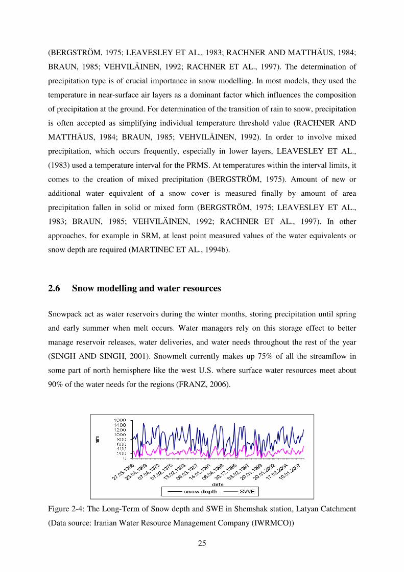
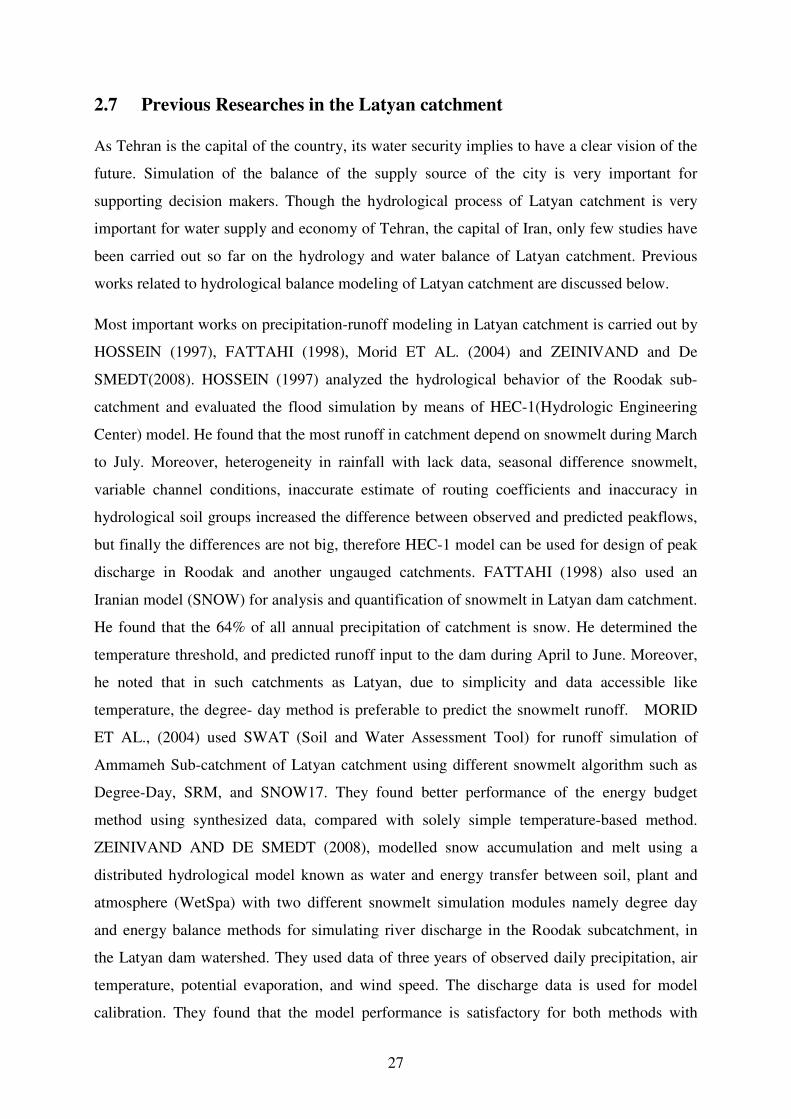
2.6 Snow modelling and water resources....................................................................... 25 2.7 Previous Researches in the Latyan catchment ......................................................... 27
3. METHODICAL APPROACH ......................................................................................... 30 3.1 Hydrological System Analysis and Delineation of Hydrological Response Units .. 31
3.1.1 Hydrological System Analysis ......................................................................... 31 3.1.1.1 Data Analysis of Hydro-Climatological Time Series ...................................... 31 3.1.1.2 Spatial Data Modelling..................................................................................... 32 3.1.2 Delineation of Hydrological Response Units................................................... 33 3.1.2.1 Concept Approach of Hydrological Response Units ....................................... 34
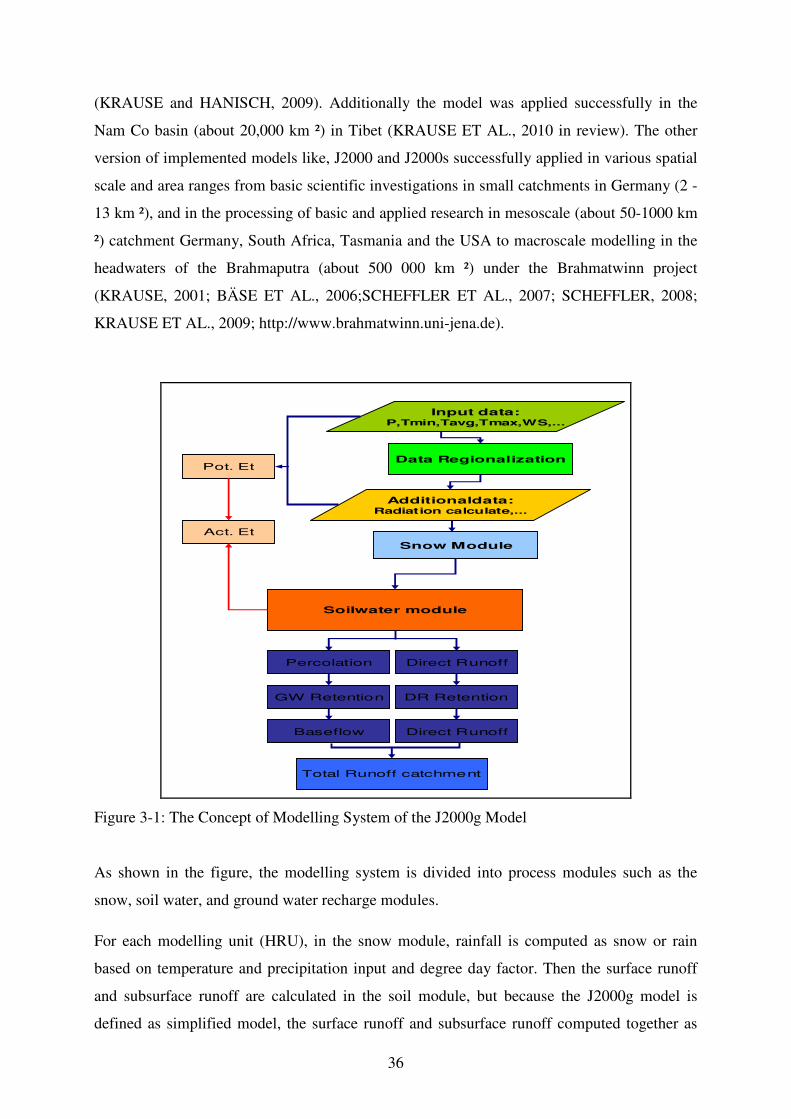
3.2 Water Balance and snowmelt-Runoff Modelling with J2000g Model .................... 35 3.2.1 The Structure of Modelling System of the J2000G Model .............................. 35 3.2.1.1 The Snow Module of the J2000g ..................................................................... 38 3.2.2 Preparation of Input Data ................................................................................. 39 3.2.3 Parameterization and Calibration ..................................................................... 41 3.2.3.1 Automatic Parameter Estimation using Sensitivity Analysis........................... 42
4. STUDY AREA AND DATA BASE................................................................................ 46 4.1 Study Area................................................................................................................ 49
4.2 Data Base.................................................................................................................. 58 4.2.1 Hydro-meteorological datasets......................................................................... 58 4.2.1.1 Precipitation Data ............................................................................................. 58
II
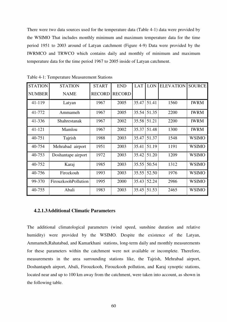
4.2.1.2 Temperature Data ............................................................................................. 59 4.2.1.3 Additional Climatic Parameters ....................................................................... 60 4.2.1.4 Runoff Data ...................................................................................................... 62 4.2.2 Spatial Datasets (GIS-Data) ............................................................................. 62
5. RESULTS AND DISCUSSION ...................................................................................... 64 5.1 System Analysis and Delineation of Hydrological Response Units ........................ 65
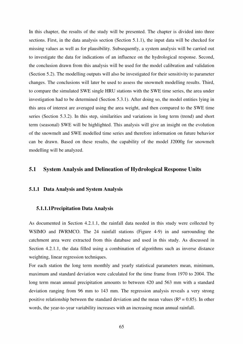
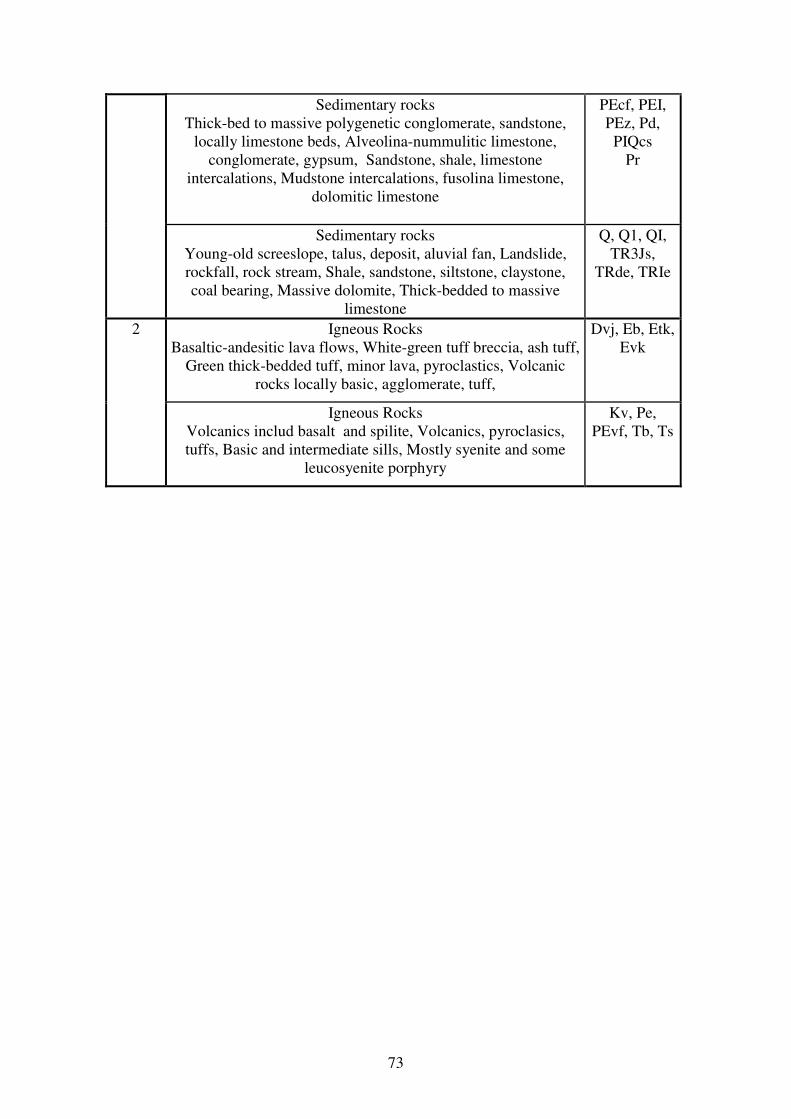
5.1.1 Data Analysis and System Analysis................................................................. 65 5.1.1.1 Precipitation Data Analysis .............................................................................. 65 5.1.1.2 Discharge Data Analysis .................................................................................. 66 5.1.1.3 Temporal Relationship between Precipitation and Discharge in the Latyan Catchment......................................................................................................................... 67 5.1.2 Spatial Dataset.................................................................................................. 69 5.1.3 Delineation of Hydrological Response Units................................................... 70 5.1.3.1 Data Preparation and Reclassification.............................................................. 70 5.1.3.2 Overlay Analysis and Reclassification ................................................... 74 5.1.3.3 Generalization and Delineation ........................................................................ 74
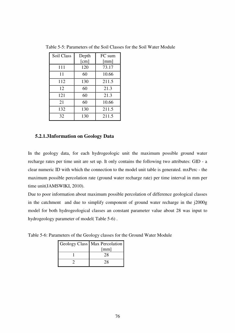
5.2 Snowmelt–Runoff Modelling using J2000g model ................................................. 74 5.2.1 Model Parameterization ................................................................................... 74 5.2.1.1 Landuse-Land Cover Information.................................................................... 75 5.2.1.2 Information on Soil Data.................................................................................. 75 5.2.1.3 Information on Geology Data .......................................................................... 76 5.2.2 Model application, calibration and evaluation ................................................. 77 5.2.2.1 Model application............................................................................................. 77 5.2.2.2 Validation ......................................................................................................... 78 5.2.2.3 Verification of the Modeling Results ............................................................... 83
6. CONCLUSIONS AND FUTURE RESEARCH.............................................................. 90 6.1 Conclusions and Future Research ............................................................................ 91
At this point, I want to take the chance to thank all those people who have directly or
indirectly contributed to the successful fulfilment of this work. Without the support, guidance
and patience of the following people this work would not have been possible.
First of all, I would like to express my deepest gratefulness to my supervisor and doctor father
Prof. Dr. Wolfgang-Albert Flügel who gave me the opportunity to write this dissertation in
Jena and for his guidance, support and advice over the last years. Again thank you so much in
advance for all. I am also grateful to Prof. Dr. Volker Hochschild who supported this work.
The discussions with him lead to the ideas that are presented in this work.
My cordial thanks go to Dr. Peter Krause, which every time his office was open for my
solving problems and discussions with him helped me a lot to work through the technical as
well as some challenging argumentative problems with my study. His constructive criticism
helped me to focus my ideas and to describe them more clearly. I am also thankful to him for
reading the some part of thesis draft within a short time period.
I appreciate the support of the Ministry of Science, Research and Technology of Iran and
Ministry of Agriculture of Iran, without whose support I could not have done my PhD in
Germany.
I am very grateful to all my colleagues of the Department for Geoinformatics, Hydrology and
Modelling, especially, Dr. Manfred Fink, Dr. Sven Kralisch, Dr. Jörg Helmschrot, Björn
Pfennig, Markus Wolf, Markus Reinhold, Christian Fischer, Franziska Zander, Christian
Schwartze, Marcel Wetzel, Daniel Varga, Frank Bäse, Hannes Müller Schmied who have
given their time to discuss pieces of my work with me and who have also offered valuable
advice. Special thanks also go to Rainer Hoffmann, the system administrator, who helped
with any occurring technical problem.
I am grateful to my friends and colleagues, Markus Reinhold, Dr. Shamsuddin Shahid, Dr.
Timothy Steele and Amanpreet Singh for proofreading and their constructive comments to
improve this dissertation.
Thanks to all agencies and institutes providing data and various support for this study: to the
AREEO staffs, in particular, Prof. Dr. Ali Ahoonmanesh, Dr. Bahram Saghafian, Dr. Kazemi,
Mr. Akbarpour, to the Iran Water Resource Management Company (IWRMCO), in particular
to Mr. Babaee, to the Iranian Revenue Operation of Dams, in particular Mr. Engineer
IV
Shahryari, to the Company of Water and Soil Engineering Service Iran (CWSESI), especially
Dr. Parehkar, Engineer Bazzaz, to the Organization of Forests and Rangelands Iran for
providing the land-cover data, to the Dr. Hossein Zeinivand in the University of Lorestan for
providing of various maps and texts of the Roodak watershed.
I would like to extend my sincere gratitude to Mrs. Dorothee Flügel for infinite supporting me
and my family throughout this whole endeavour. I would not have gone so far without her
unfailing support and encouragement.
Many thank for short but very valuable financial support from the Jenaer Graduate Academy
the University of Friedrich-Schiller Jena.
I want to thank all my friends -- in particular, Dr. Osman Azizi, Ebrahim Amini, Dr. Ebrahim
Fattahi, Engineer David Alamshah, Dr. Mousa Kamanroodi, Dr. Farhad Azizpour, Dr. You
Qinglong, Santosh Nepal and Engineer Taher Pasbani.
My sincere thanks to my father-in-low, that without his continuous and encouraging support I
could not finish my PhD.
Special thanks go to my dear parents and to my sisters and brothers for their endless support
and the trust in me.
The making of the thesis was dominated by a time full of privation, not only for the author,
but especially for my family. The success and continuity of the work originated form the
never ending support of them. Many thanks go especially to my wife, who had to suffer under
the evening and weekends full of work. Through her understanding and loving nature and her
encouragements, she helped to finish this work successfully.
V
LISTS OF FIGURES
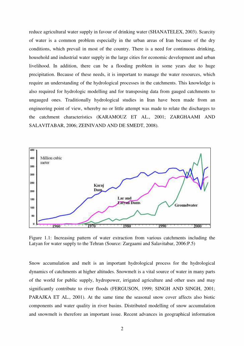
Figure 1.1: Increasing pattern of water extraction from various catchments including the
Latyan for water supply to the Tehran 02
Figure2-1: The Global Water Cycle 07
Figure 2-2: The Global freshwater and role of snow 07
Figure 2-3: Schematic representation of typical hydrograph curves of melt runoff in selected
Central European region 16
Figure 2-4:The long term of Snow depth and SWE in Shemshak station, Latyan catchment 25
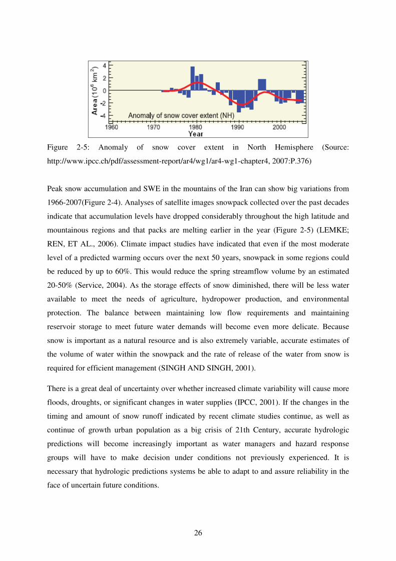
Figure 2-5: Anomaly of snow cover extent in North Hemisphere 26
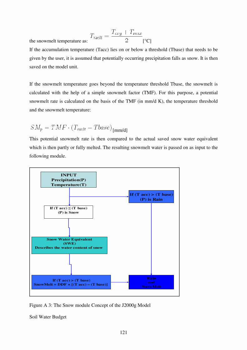
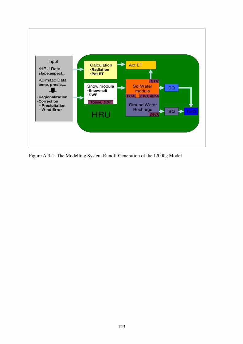
Figure 3-1: The Concept of Modelling System of the J2000g Model 36
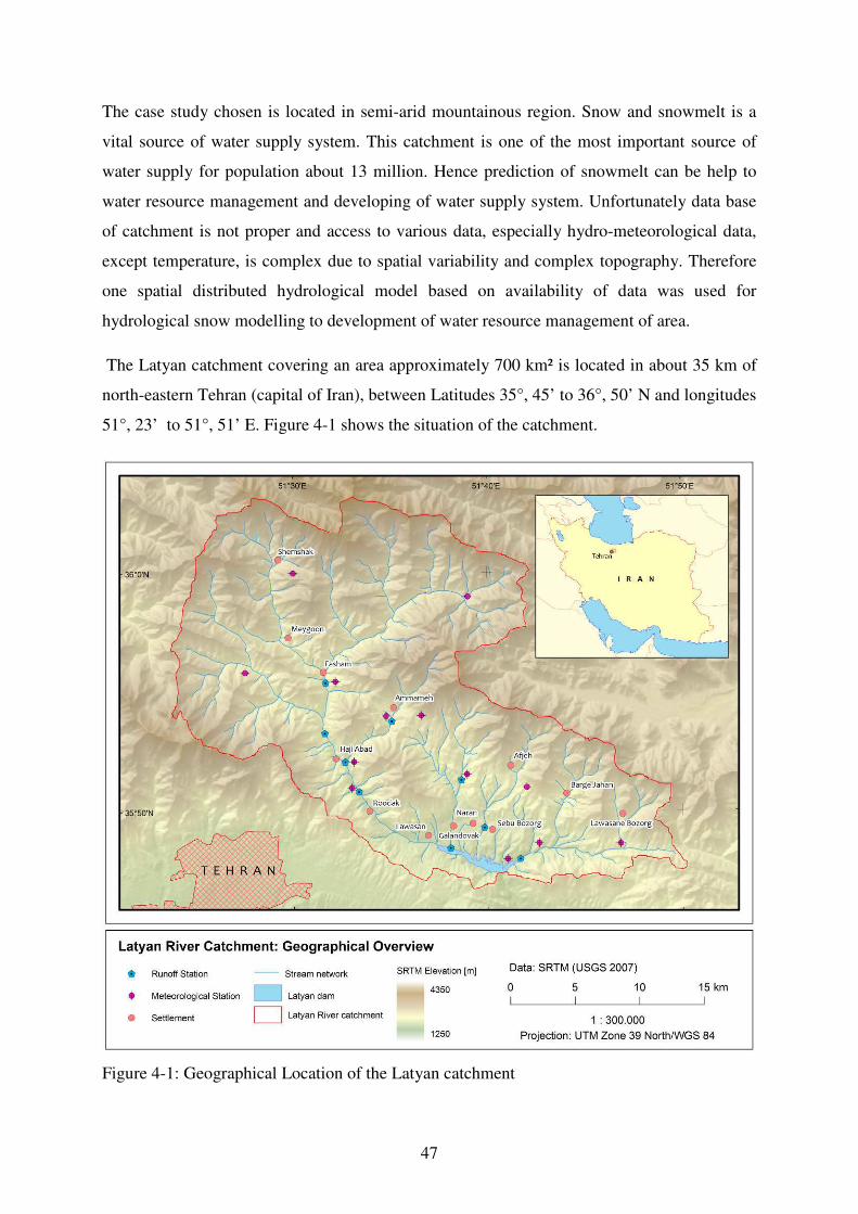
Figure 4-1: Geographical Location of the Latyan catchment 47
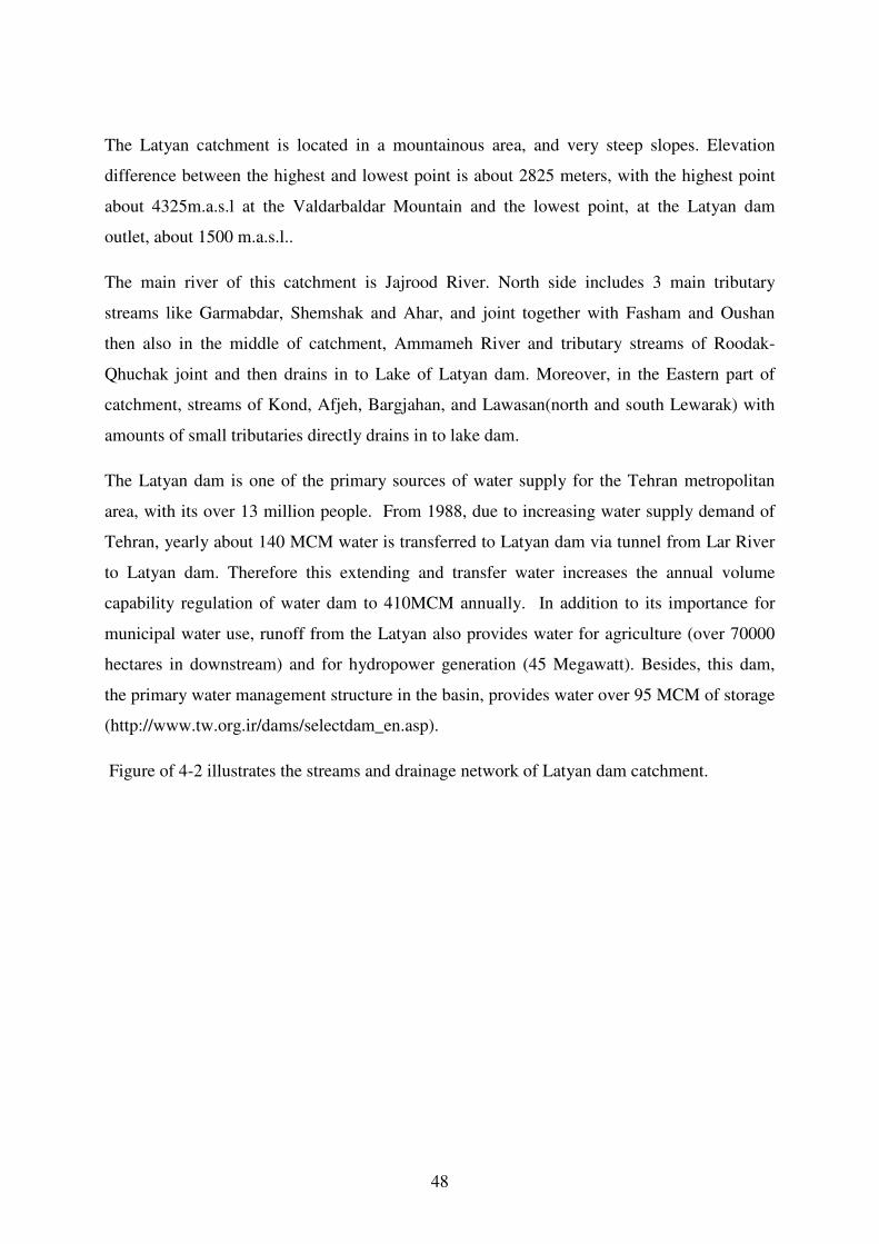
Figure 4-2: Streams and Network and Subcatchments of the Latyan Catchment 49
Figure4-3: Mean Annual (1967-2007) Monthly Precipitation in the Latyan Catchment 51
Figure 4-4: Mean Annual (1967-2007) Monthly Precipitation in the Latyan Catchment 51
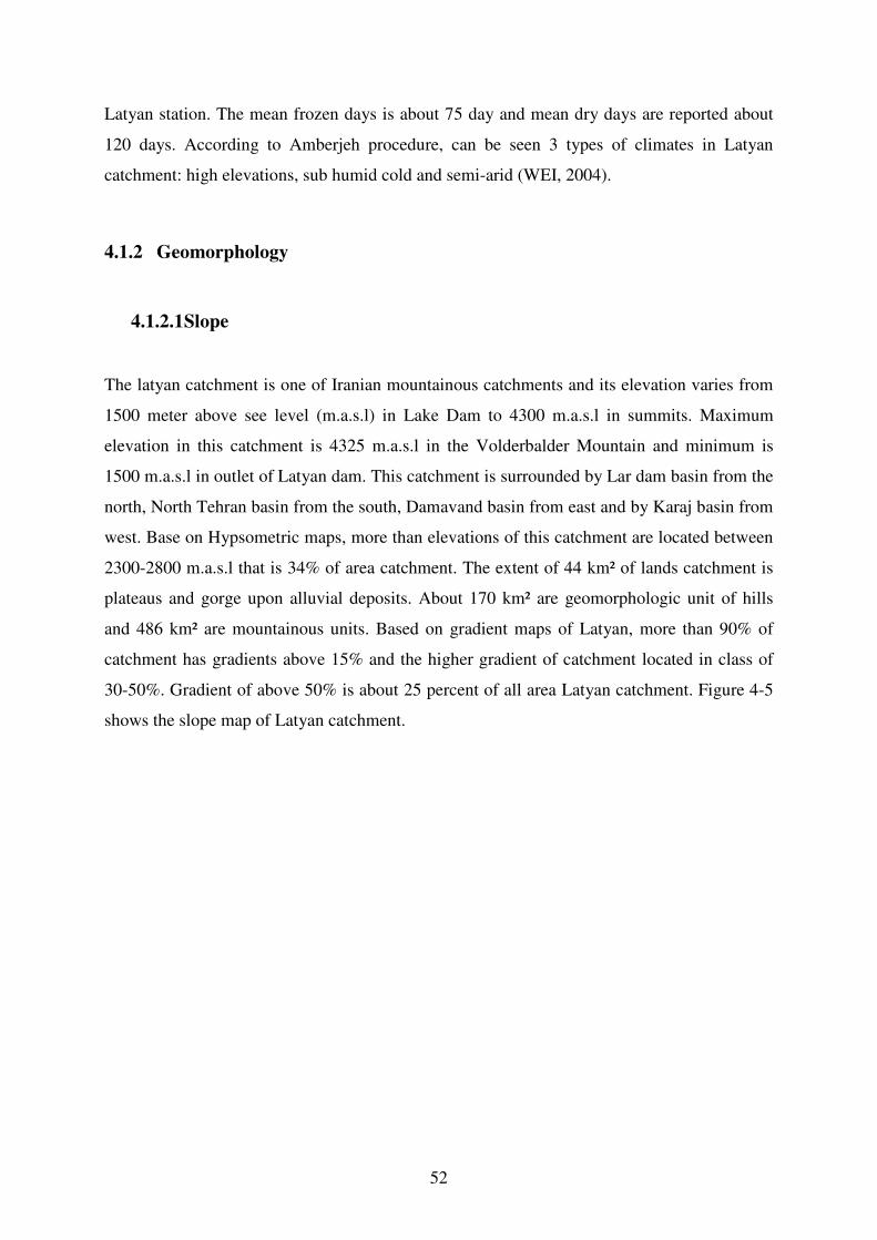
Figure 4-5: Slope Classes in the Latyan Catchment 53
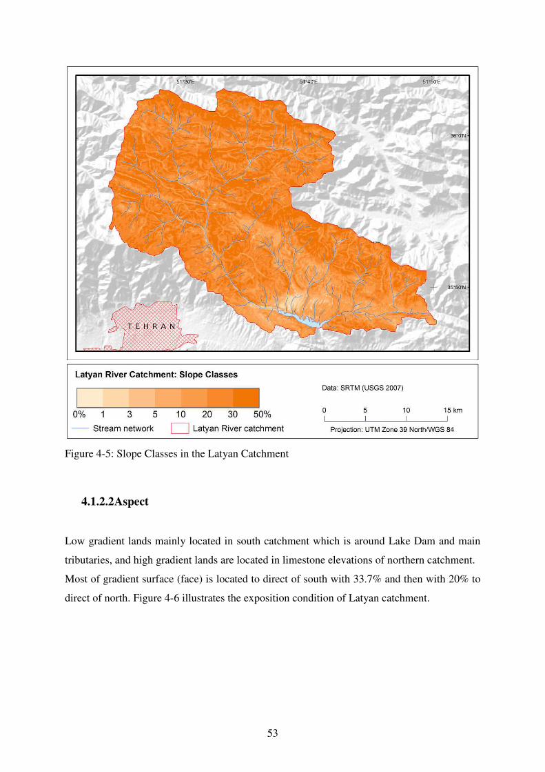
Figure 4-6: exposition condition of the Latyan Catchment 54
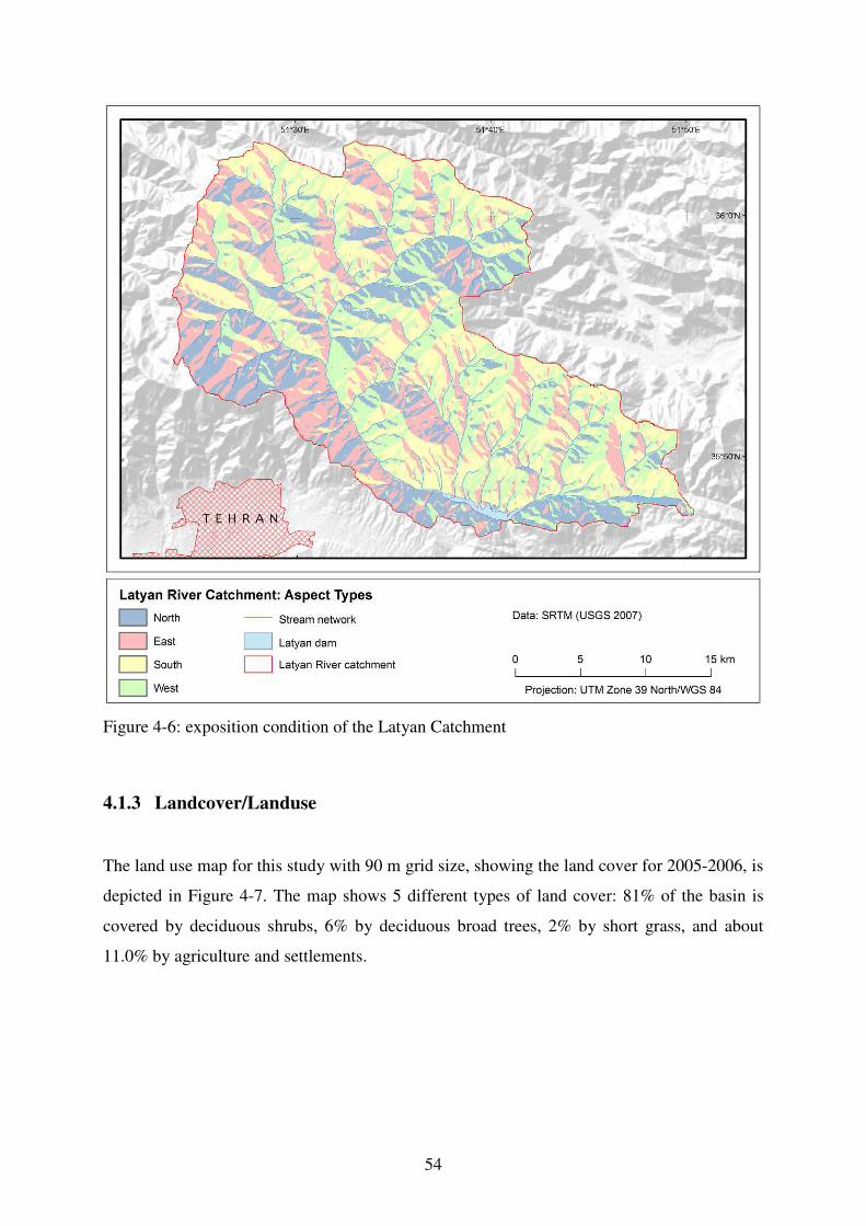
Figure 4-7: Landcover/Landuse of the Latyan Catchment 55
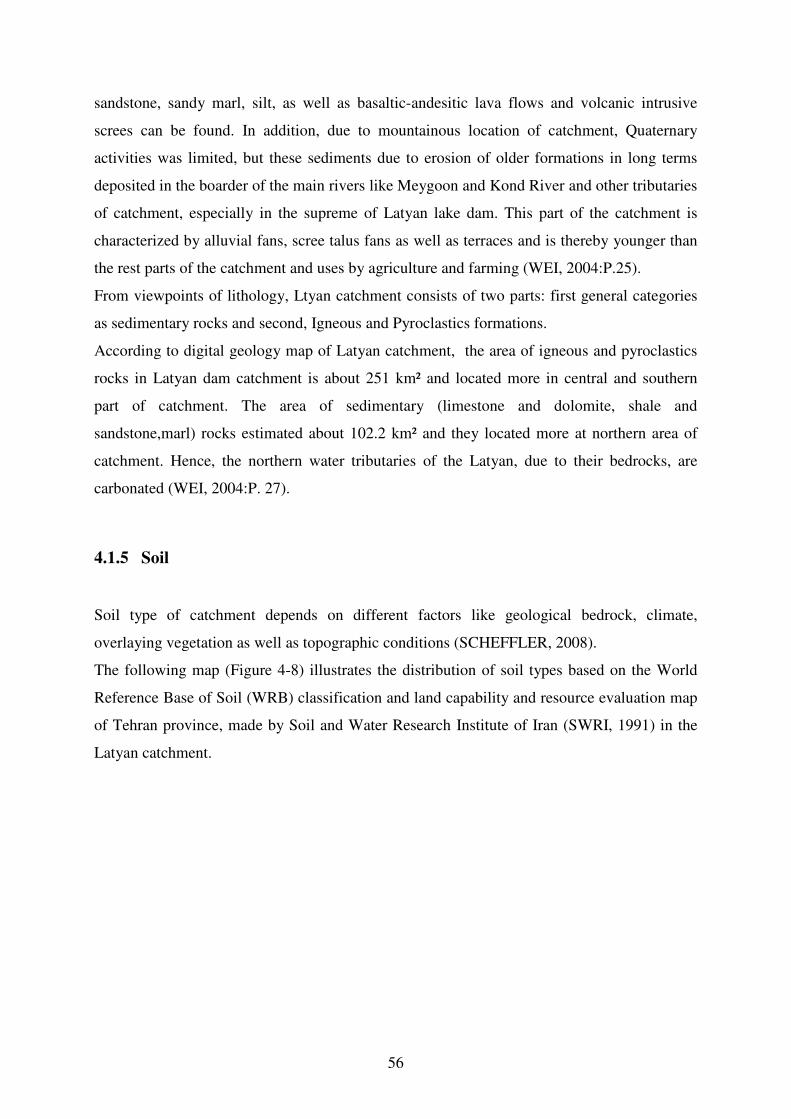
Figure 4-8: Soil Types Map of the Latyan Catchment 57
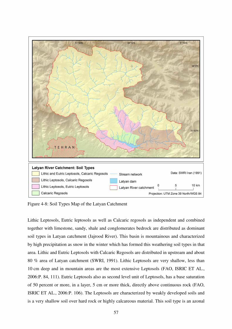
Figure4-9:The Location of Meteorological stations inside and around the Latyan catchment59
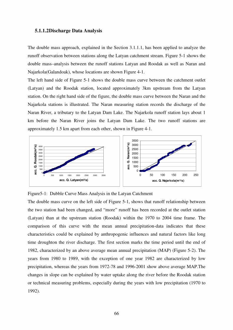
Figure5-1: Dubble Curve Mass Analysis in the Latyan Catchment 66
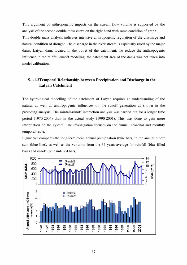
Figure 5-2: The 34 years Evaluations of rainfall and Runoff in the Latyan catchment 67
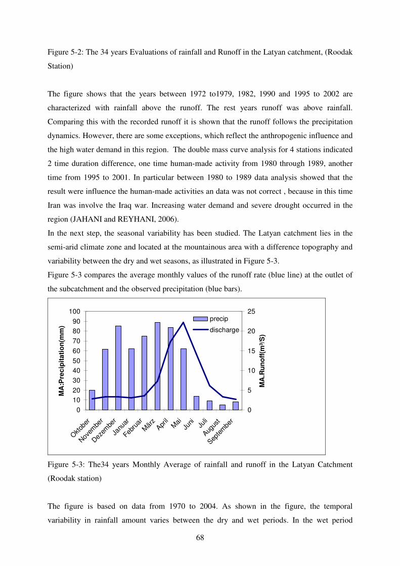
Figure 5-3: The34 years Monthly Average of rainfall and runoff in the Latyan Catchment 68
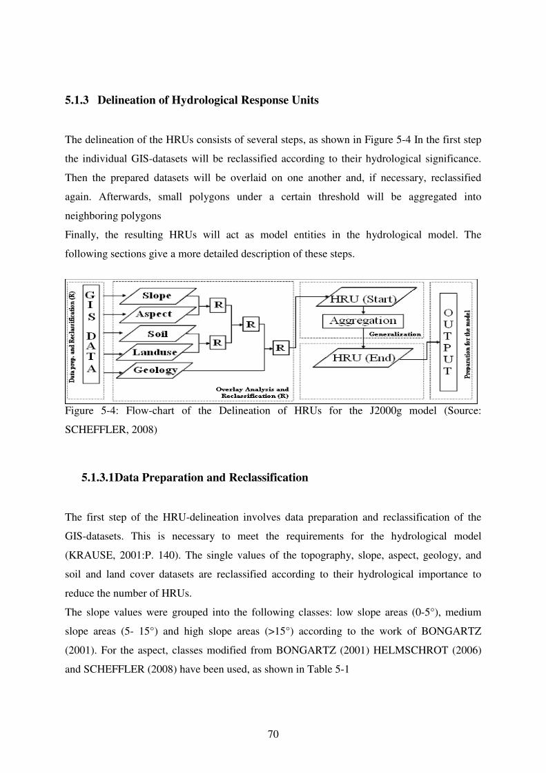
Figure 5-4: Flow-chart of the Delineation of HRUs for the J2000g model 70
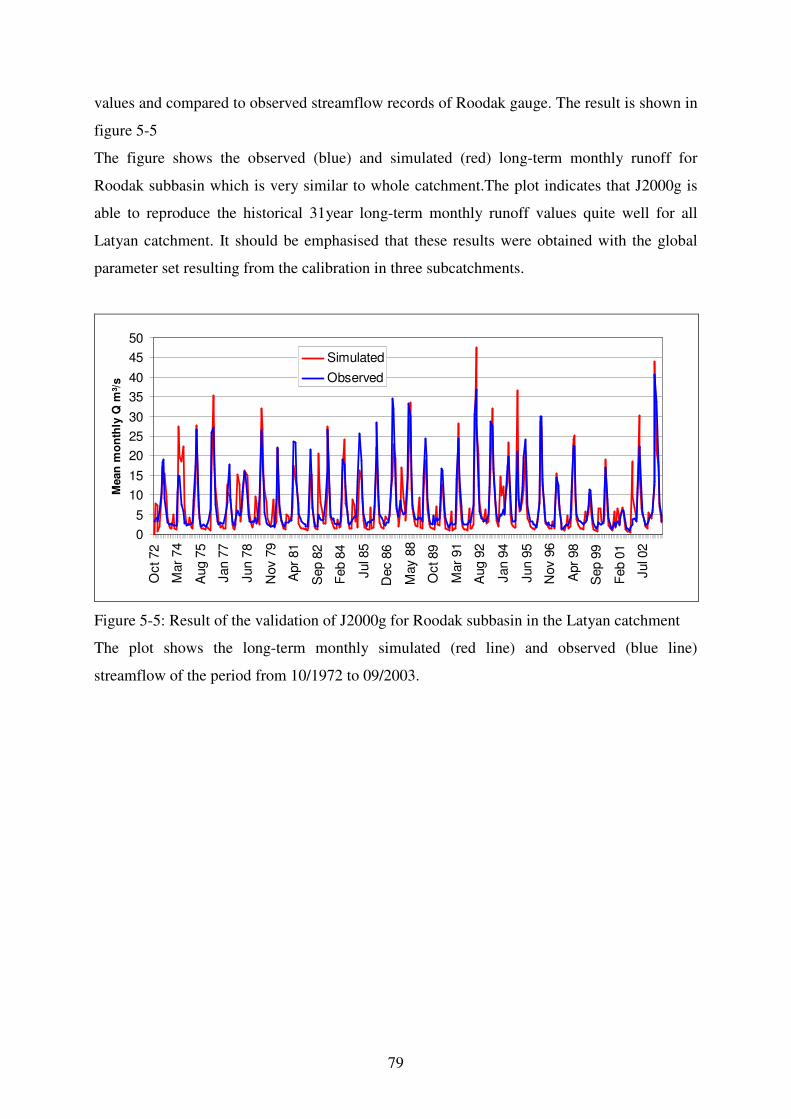
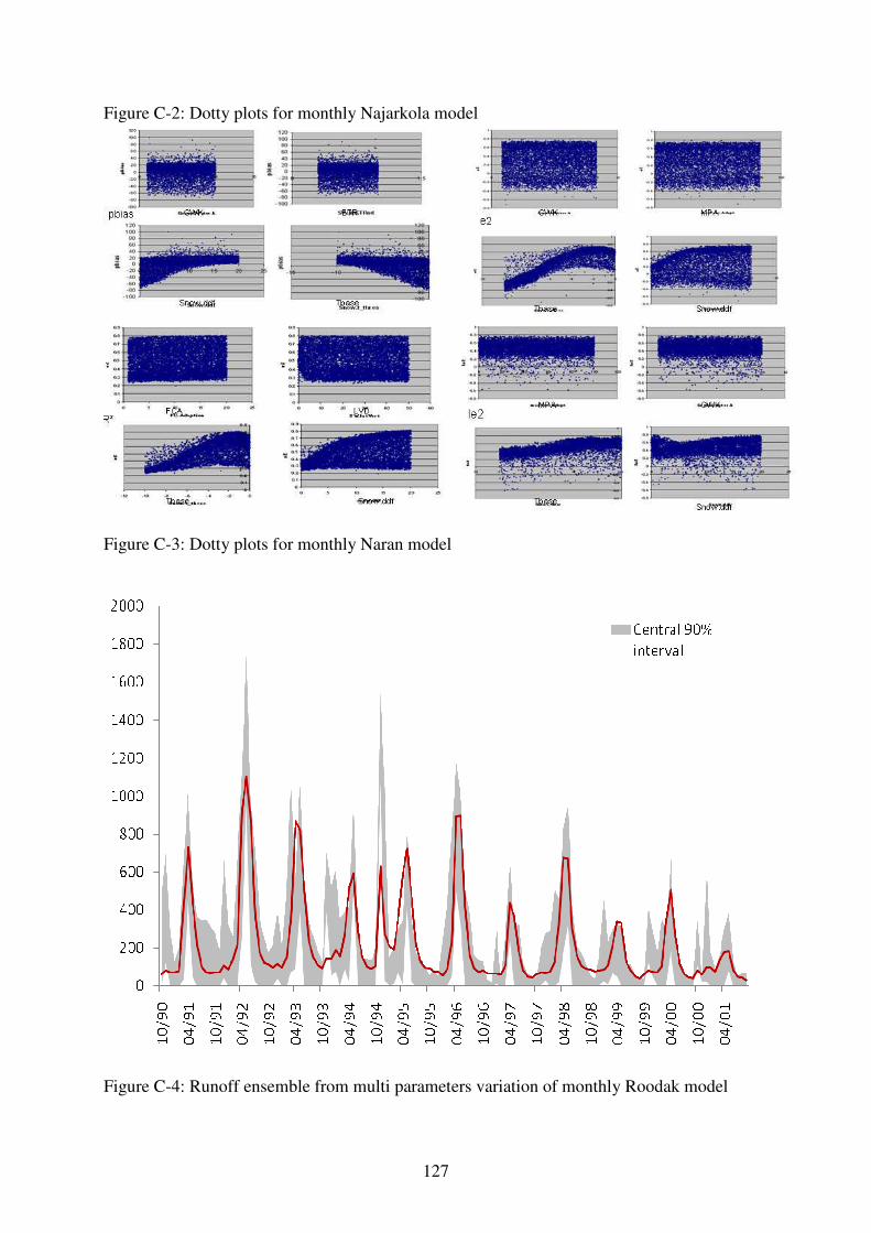
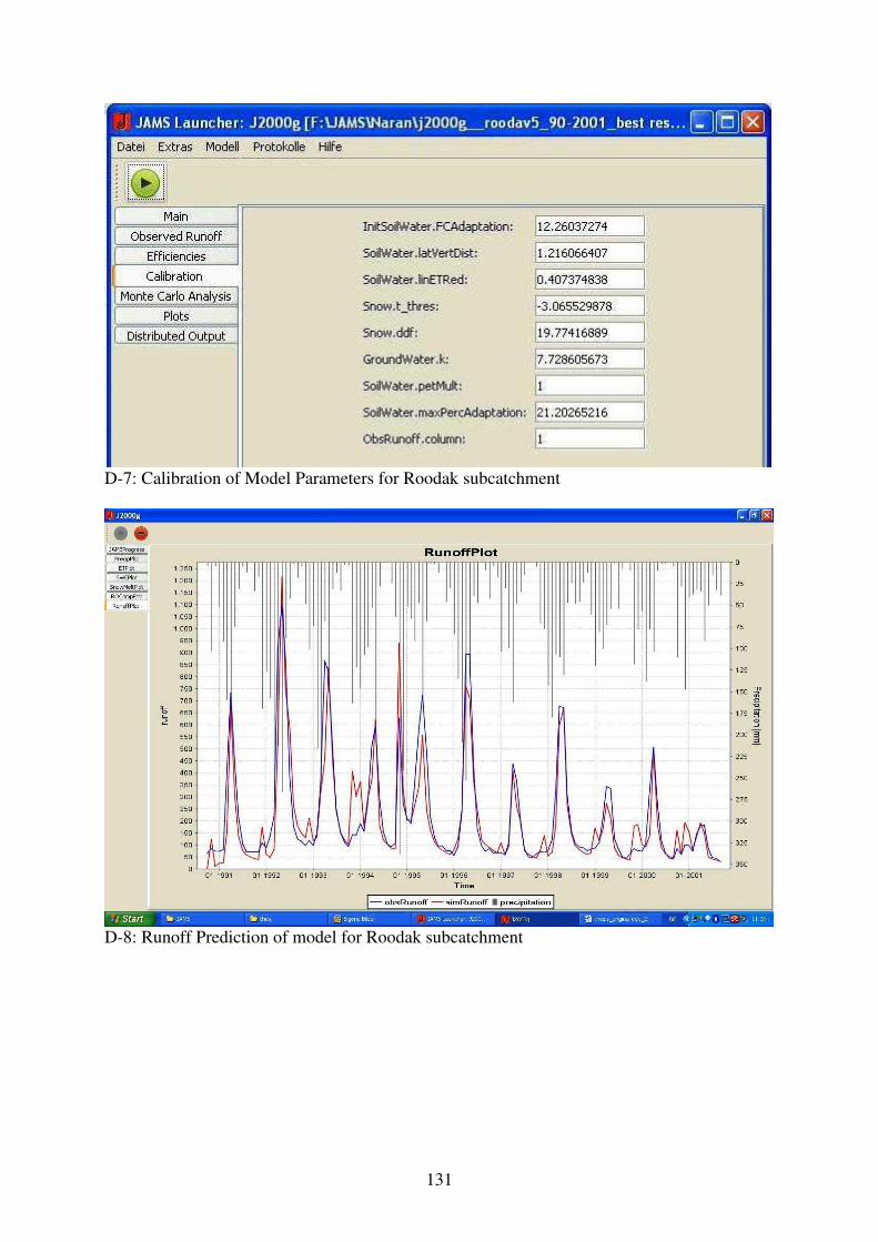
Figure 5-5:Result of the validation of J2000g for Roodak subbasin in the Latyan catchment79
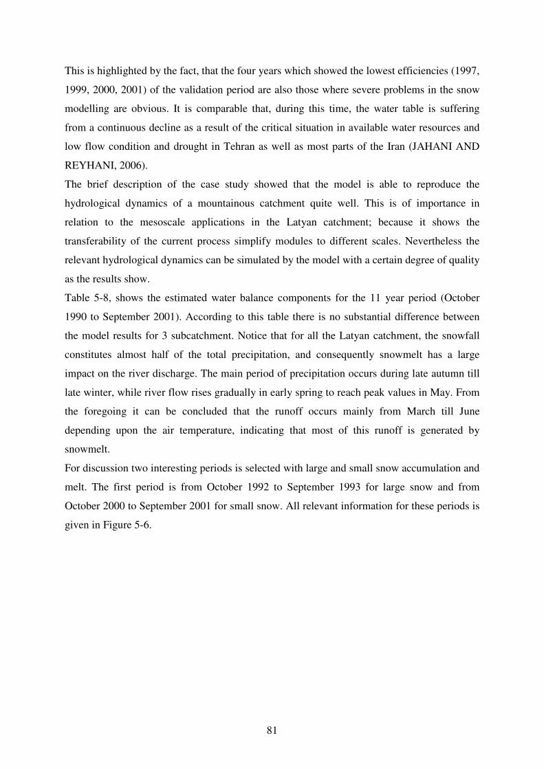
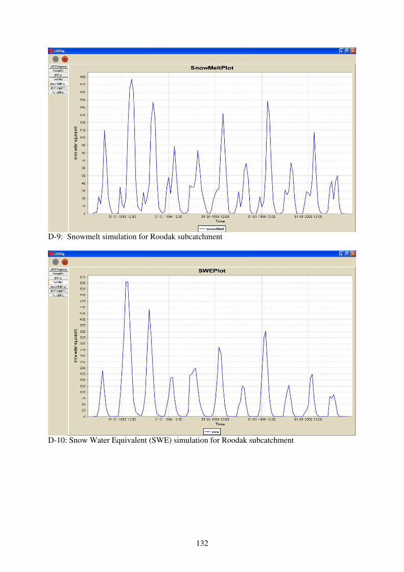
Figure 5-6: Monthly precipitation, mean air temperature, snow water equivalent and
snowmelt, Roodak subbasin, J2000g model simulation, 1992-1993. 82
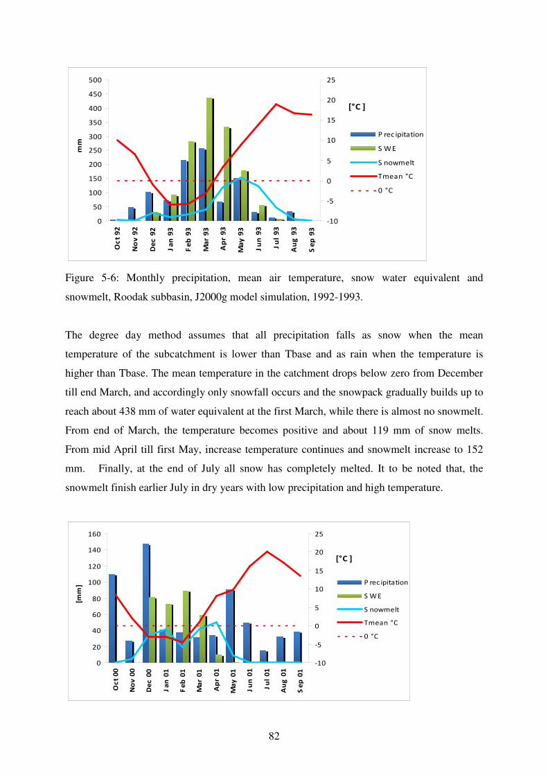
Figure 5-7: Monthly precipitation, mean air temperature, snow water equivalent and
snowmelt, Roodak subbasin, J2000g model simulation, 2000-2001 82
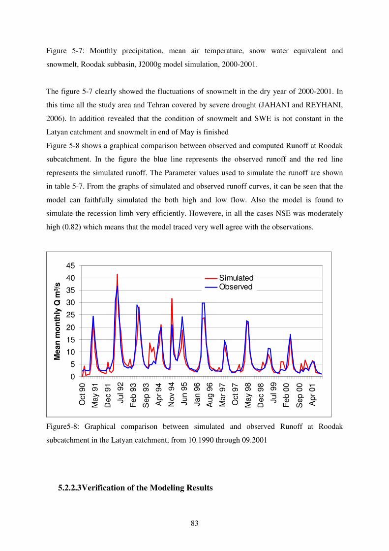
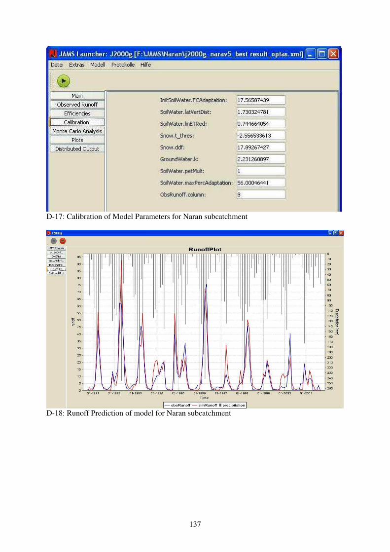
Figure5-8: Graphical comparison between simulated and observed Runoff at Roodak
subcatchment in the Latyan catchment, from 10.1990 through 09.2001 83
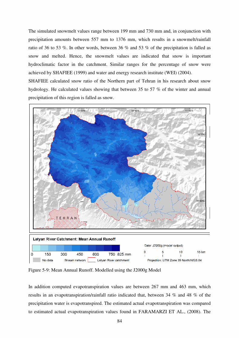
Figure 5-9: Mean Annual Runoff. Modelled using the J2000g Model 84
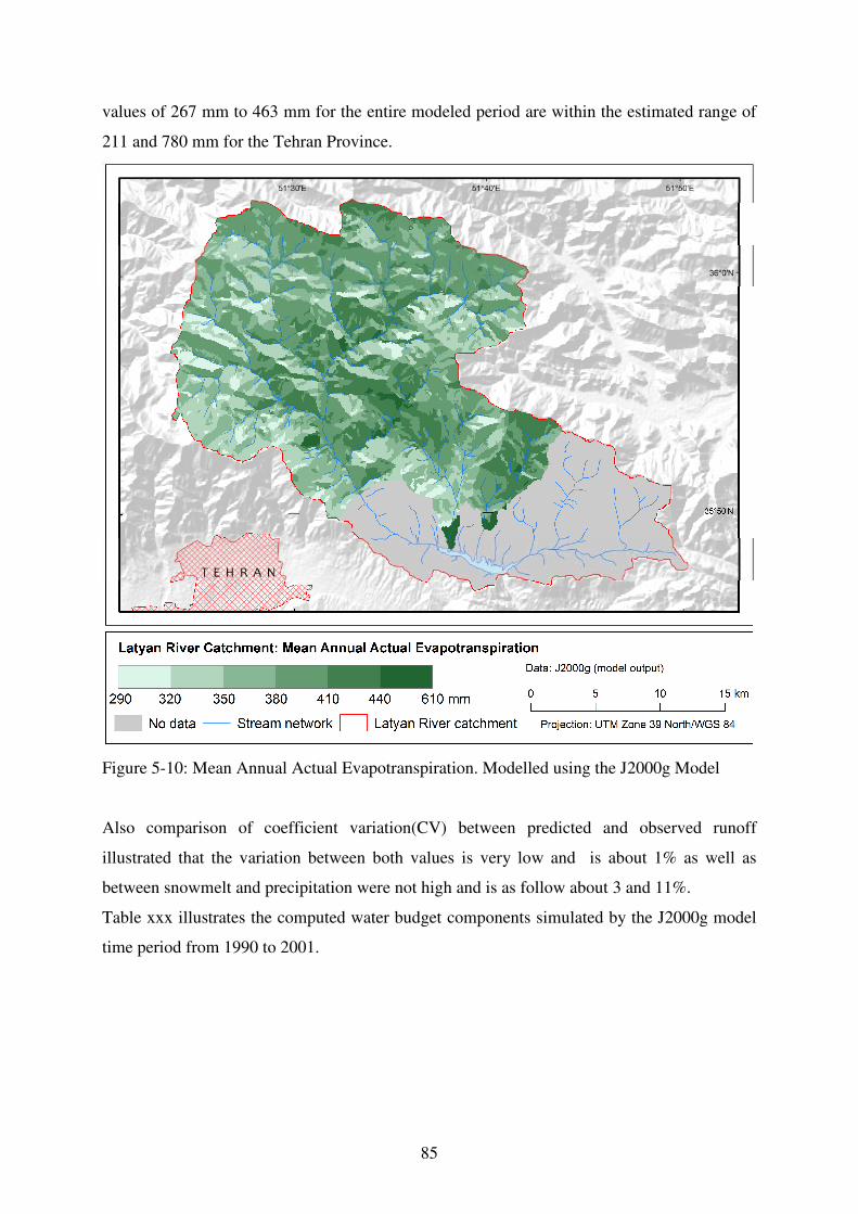
Figure 5-10: Mean Annual Actual Evapotranspiration. Modelled using the J2000g Model 85
VI
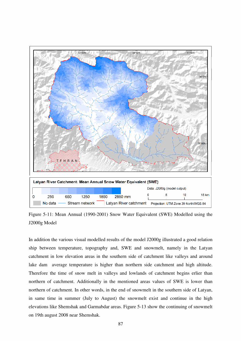
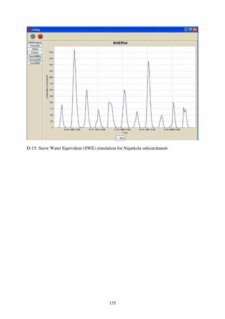
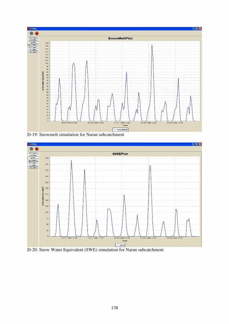
Figure 5-11: Mean Annual (1990-2001) Snow Water Equivalent (SWE) Modelled using the
J2000g Model 87
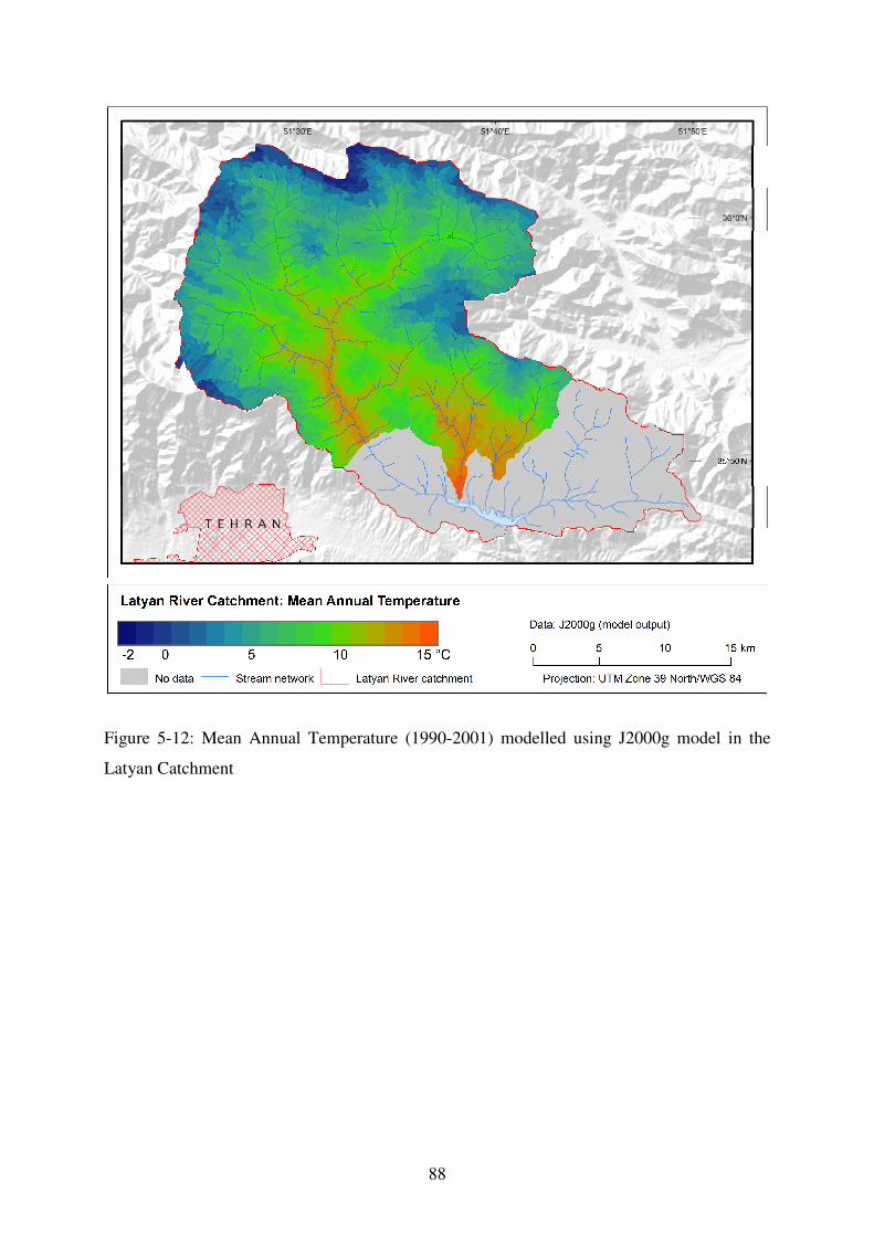
Figure 5-12: Mean Annual Temperature (1990-2001) modelled using J2000g model in the
Latyan Catchmet 88
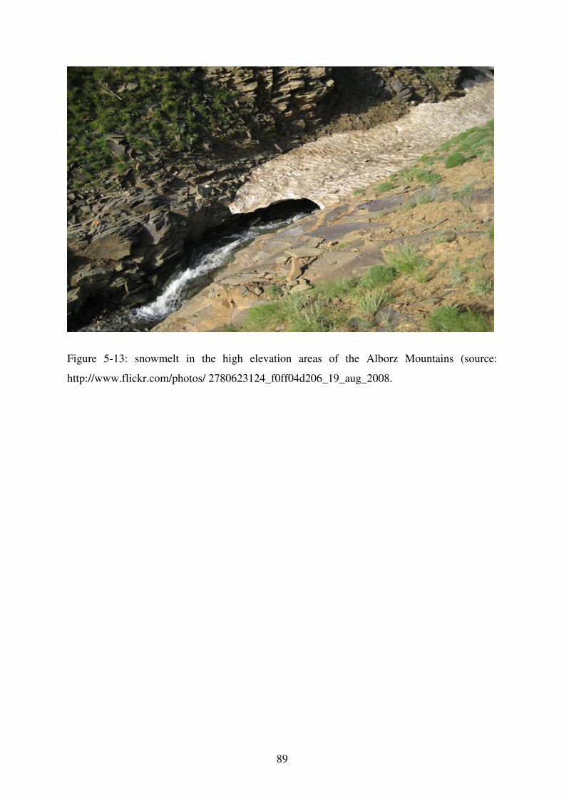
Figure 5-13: snowmelt in the high elevation areas of the Alborz Mountains 89
VII
LISTS OF TABLES
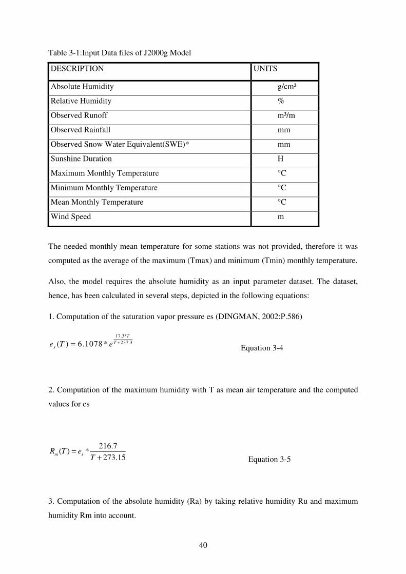
Table 3-1:Input Data files of J2000g Model 40
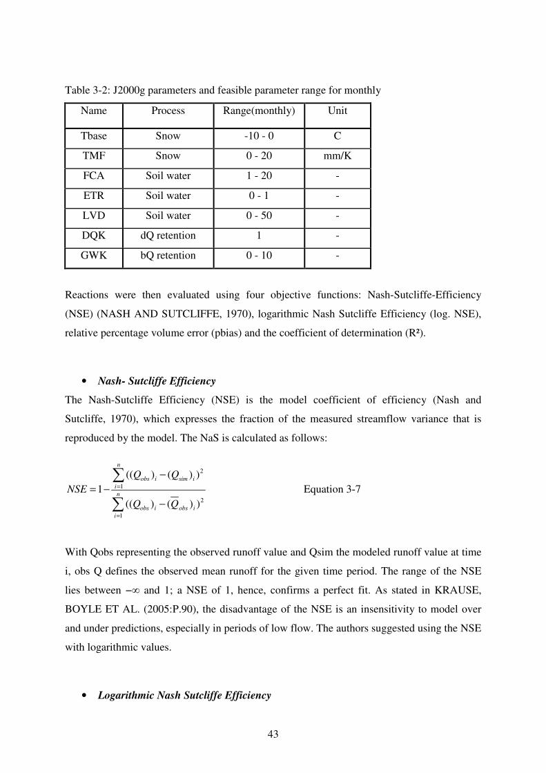
Table 3-2: J2000g parameters and feasible parameter range for monthly 43
Table 4-1: Temperature Measurement Stations 60
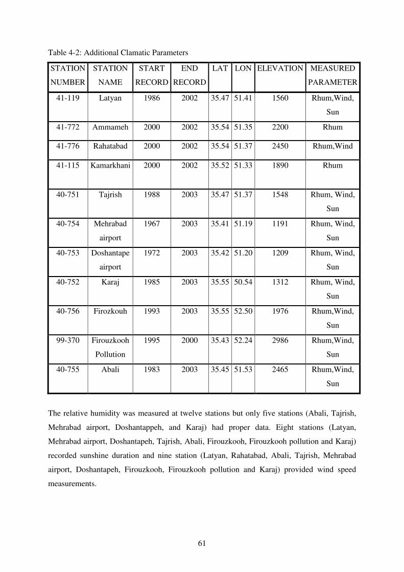
Table 4-2: Additional Clamatic Parameters 61
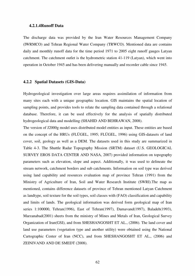
Table 4-3: GIS-dataset for HRU- delineation 63
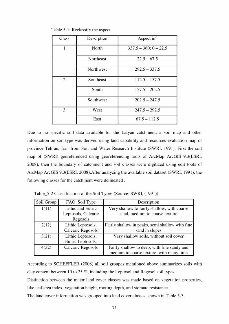
Table 5-1: Reclassify the aspect 71
Table 5-2 Classification of the Soil Types 71
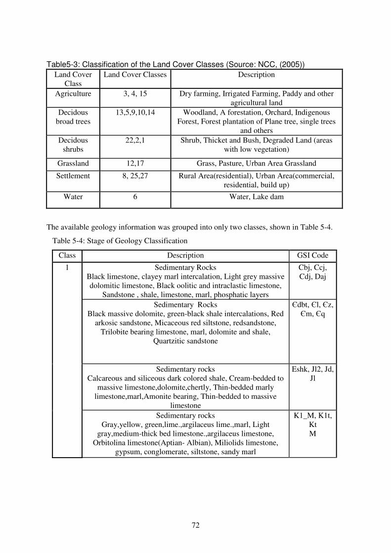
Table5-3: Classification of the Land Cover Classes 72
Table 5-4: Stage of Geology Classification 72
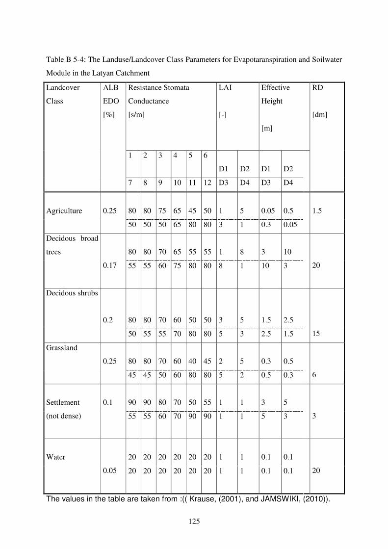
Table 5-5: Parameters of the Soil Classes for the Soil Water Module 76
Table 5-6: Parameters of the Geology classes for the Ground Water Module 76
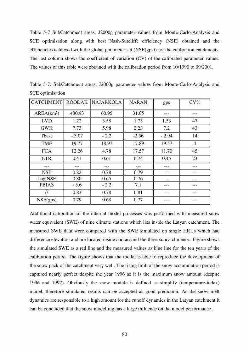
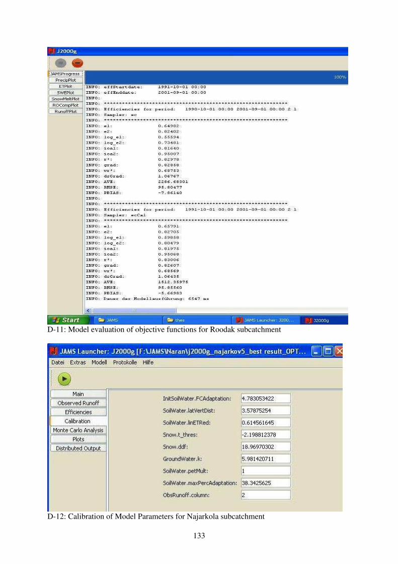
Table 5-7: SubCatchment areas, J2000g parameter values from Monte-Carlo-Analysis and
SCE optimisation 80
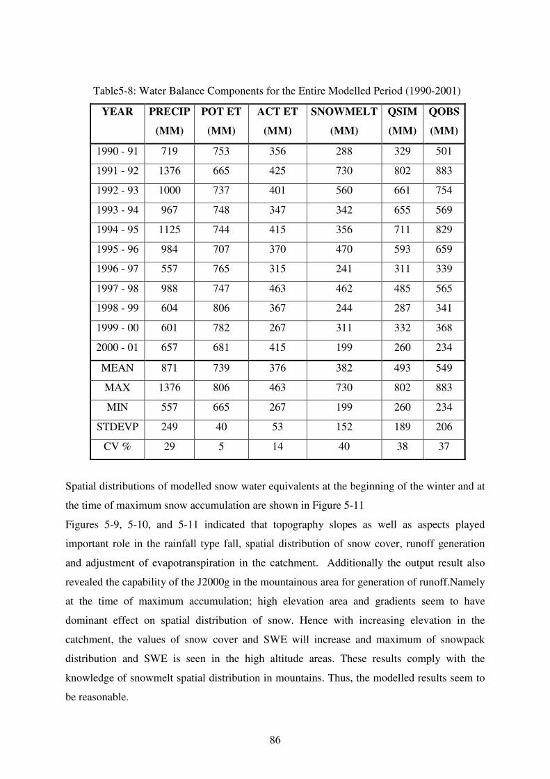
Table5-8: Water Balance Components for the Entire Modelled Period (1990-2001) 86
VIII
ABBREVIATIONS
ABBREVIATION DESCRIPTION
AC Air Capacity
AET Actual Evapotranspiration
Alb Albedo
ASA Aggregated Simulation Area
AVE Absolute Volume Error
AVG Average
D Depth
DHI Danish Hydraulic Institute
E East
FAO Food and Agriculture Organization of the United Nations
FCA Field Capacity Adaption
GCM General Circulation Model
GIS Geographical Information System
GSI Geological Survey Organization Iran
HRU Hyrological Response Units
HBV Hydrologiska Byråns Vattenbalansavdelning model
HEC-1 Hydrologic Engineering Center
HSPF Hydrological Simulation Program - FORTRAN
ICSI International Commission on Snow and Ice
IDW Inverse Distance Weighting
IPCC Intergovernmental Panel on Climate Change
ISRIC International Soil Reference and Information Centre
IWRMCO Iran Water Resource Management Company
JAMS Jena Adaptable Modeling System
LAI Leaf Area Index
LAT Latitude
Log.NSE Logarithmic Nash-Sutcliffe Efficiency
LON Longitude
LSS Land cover Soil Sets
IX
MAP Mean Annual Precipitation
MAR Mean Annual Runoff
MASL Meter Above See Level
MCM Million Cubic Meter
MMS Modular Modeling System
N North
NCC National Cartographic Center
NSE Nash Sutclif
OBS Observation
P Precipitation
PBIAS relative percentage volume error
PET Potential Evapotranspiration
PRMS Precipitation-Runoff Modeling System
Q Discharge
R² coefficient of determination
Rd Roothing Depth
Rhum Relative Humidity
RS Remote Sensing
RU Response Unit
S South
SC Soil Class
SIM Simulation
SLURP Semi-distributed Land Use-based Runoff Processes
SMHI Swedish Meteorological and Hydrological Institute
SRTM Shuttle Radar Topography Mission
SRM Snow Runoff Model
STDEVP Standard Deviation Population
SUN Sunshine duration
SVAT Soil-Vegetation-Atmosphere-Transfer
SWE Snow Water Equivalent
SWRI Soil Water Research Institute
TIN triangulated irregular network
X
TS Topography Sets
TWRCO Tehran Water Regional Company
USGS US Geological Survey
UTM Universal Transverse Mercator
VSC Vegetation Soil Complex
W West
WASIM Water balance Simulation Model
WEI Water and Energy Institute
WMO World Meteorological Organization
WRB World Reference Base for Soil Resources
WSIMO Weather Service Iran Meteorological Organization
XI
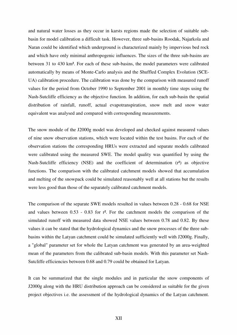
Abstract
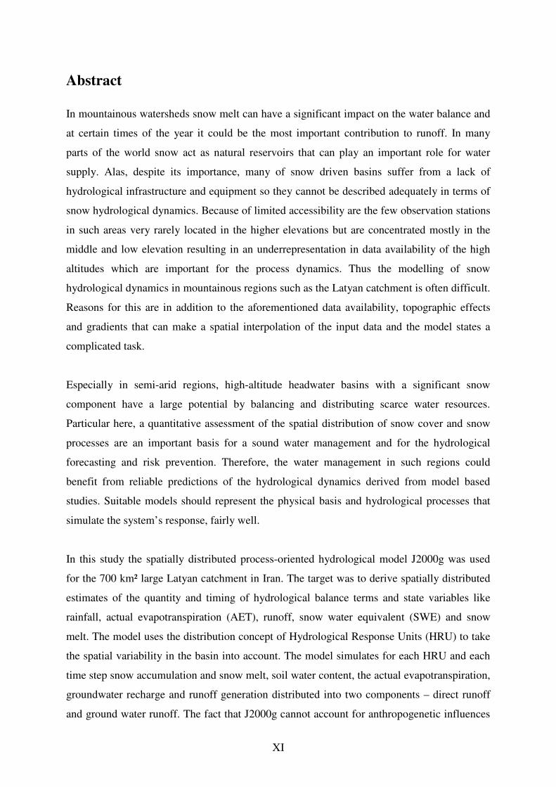
In mountainous watersheds snow melt can have a significant impact on the water balance and
at certain times of the year it could be the most important contribution to runoff. In many
parts of the world snow act as natural reservoirs that can play an important role for water
supply. Alas, despite its importance, many of snow driven basins suffer from a lack of
hydrological infrastructure and equipment so they cannot be described adequately in terms of
snow hydrological dynamics. Because of limited accessibility are the few observation stations
in such areas very rarely located in the higher elevations but are concentrated mostly in the
middle and low elevation resulting in an underrepresentation in data availability of the high
altitudes which are important for the process dynamics. Thus the modelling of snow
hydrological dynamics in mountainous regions such as the Latyan catchment is often difficult.
Reasons for this are in addition to the aforementioned data availability, topographic effects
and gradients that can make a spatial interpolation of the input data and the model states a
complicated task.
Especially in semi-arid regions, high-altitude headwater basins with a significant snow
component have a large potential by balancing and distributing scarce water resources.
Particular here, a quantitative assessment of the spatial distribution of snow cover and snow
processes are an important basis for a sound water management and for the hydrological
forecasting and risk prevention. Therefore, the water management in such regions could
benefit from reliable predictions of the hydrological dynamics derived from model based
studies. Suitable models should represent the physical basis and hydrological processes that
simulate the system’s response, fairly well.
In this study the spatially distributed process-oriented hydrological model J2000g was used
for the 700 km² large Latyan catchment in Iran. The target was to derive spatially distributed
estimates of the quantity and timing of hydrological balance terms and state variables like
rainfall, actual evapotranspiration (AET), runoff, snow water equivalent (SWE) and snow
melt. The model uses the distribution concept of Hydrological Response Units (HRU) to take
the spatial variability in the basin into account. The model simulates for each HRU and each
time step snow accumulation and snow melt, soil water content, the actual evapotranspiration,
groundwater recharge and runoff generation distributed into two components – direct runoff
and ground water runoff. The fact that J2000g cannot account for anthropogenetic influences
XII
and natural water losses as they occur in karsts regions made the selection of suitable sub-
basin for model calibration a difficult task. However, three sub-basins Roodak, Najarkola and
Naran could be identified which underground is characterized mainly by impervious bed rock
and which have only minimal anthropogenic influences. The sizes of the three sub-basins are
between 31 to 430 km². For each of these sub-basins, the model parameters were calibrated
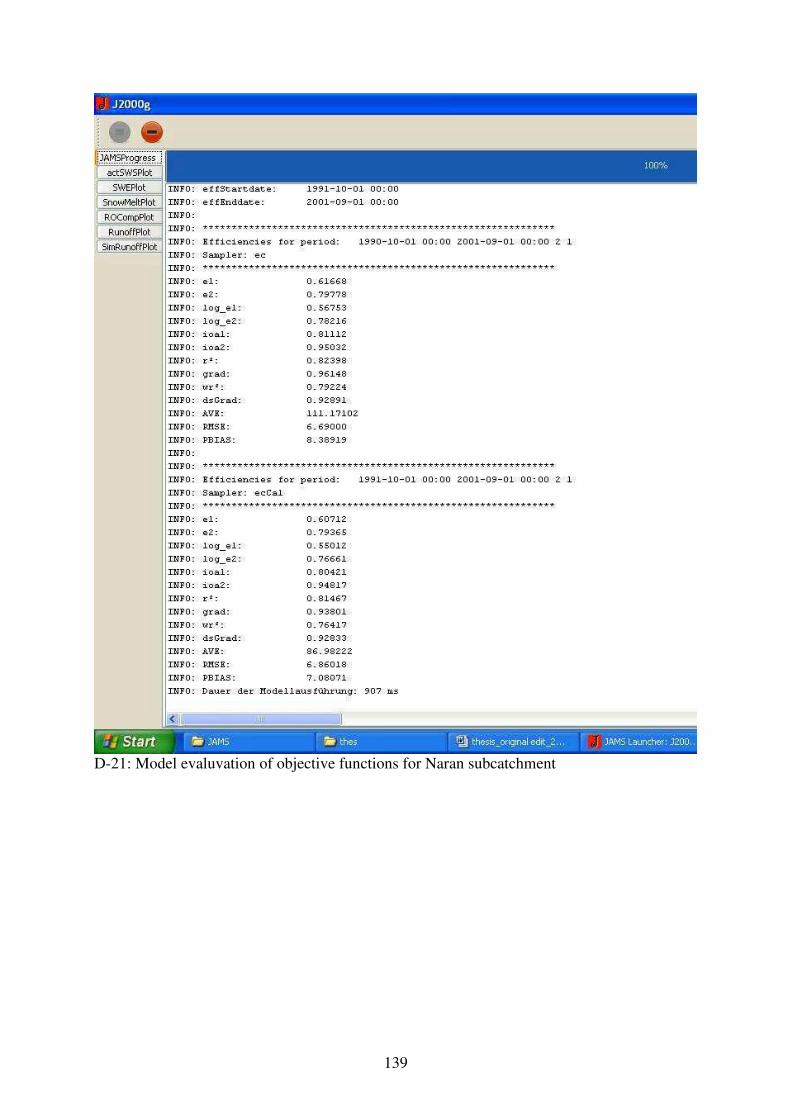
automatically by means of Monte-Carlo analysis and the Shuffled Complex Evolution (SCE-
UA) calibration procedure. The calibration was done by the comparison with measured runoff
values for the period from October 1990 to September 2001 in monthly time steps using the
Nash-Sutcliffe efficiency as the objective function. In addition, for each sub-basin the spatial
distribution of rainfall, runoff, actual evapotranspiration, snow melt and snow water
equivalent was analysed and compared with corresponding measurements.
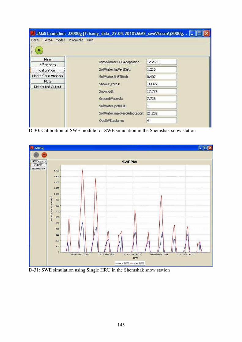
The snow module of the J2000g model was developed and checked against measured values
of nine snow observation stations, which were located within the test basins. For each of the
observation stations the corresponding HRUs were extracted and separate models calibrated
were calibrated using the measured SWE. The model quality was quantified by using the
Nash-Sutcliffe efficiency (NSE) and the coefficient of determination (r²) as objective
functions. The comparison with the calibrated catchment models showed that accumulation
and melting of the snowpack could be simulated reasonably well at all stations but the results
were less good than those of the separately calibrated catchment models.
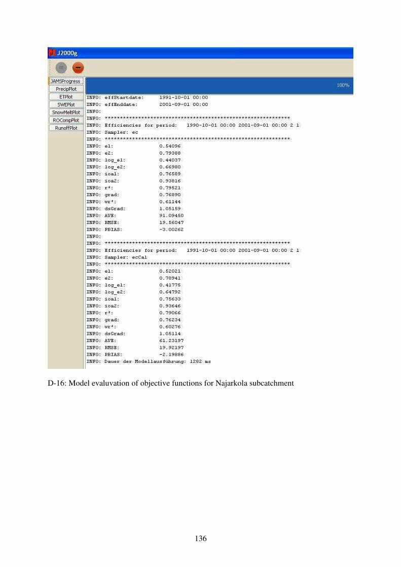
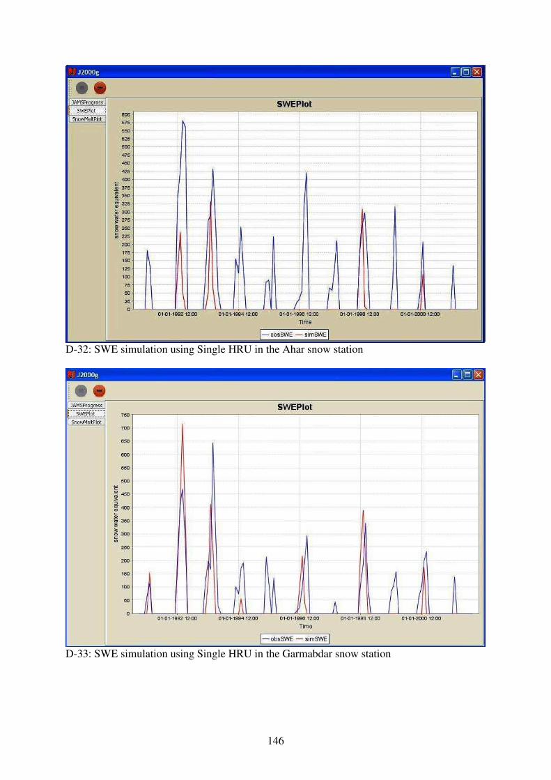
The comparison of the separate SWE models resulted in values between 0.28 - 0.68 for NSE
and values between 0.53 - 0.83 for r². For the catchment models the comparison of the
simulated runoff with measured data showed NSE values between 0.78 and 0.82. By these
values it can be stated that the hydrological dynamics and the snow processes of the three sub-
basins within the Latyan catchment could be simulated sufficiently well with J2000g. Finally,
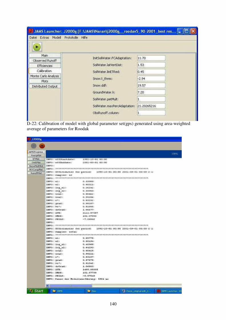
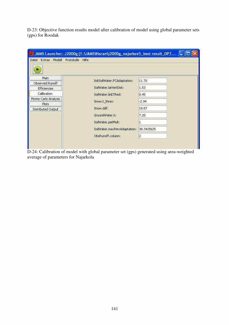
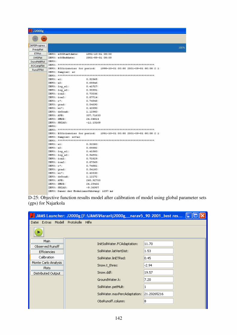
a "global" parameter set for whole the Latyan catchment was generated by an area-weighted
mean of the parameters from the calibrated sub-basin models. With this parameter set Nash-
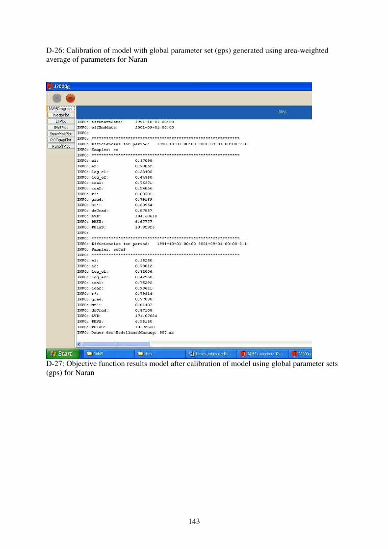
Sutcliffe efficiencies between 0.68 and 0.79 could be obtained for Latyan.
It can be summarized that the single modules and in particular the snow components of
J2000g along with the HRU distribution approach can be considered as suitable for the given
project objectives i.e. the assessment of the hydrological dynamics of the Latyan catchment.
XIII
Hereby, the model can be used to elaborate important hydrological information for a
sustainable management of the water resources.
XIV
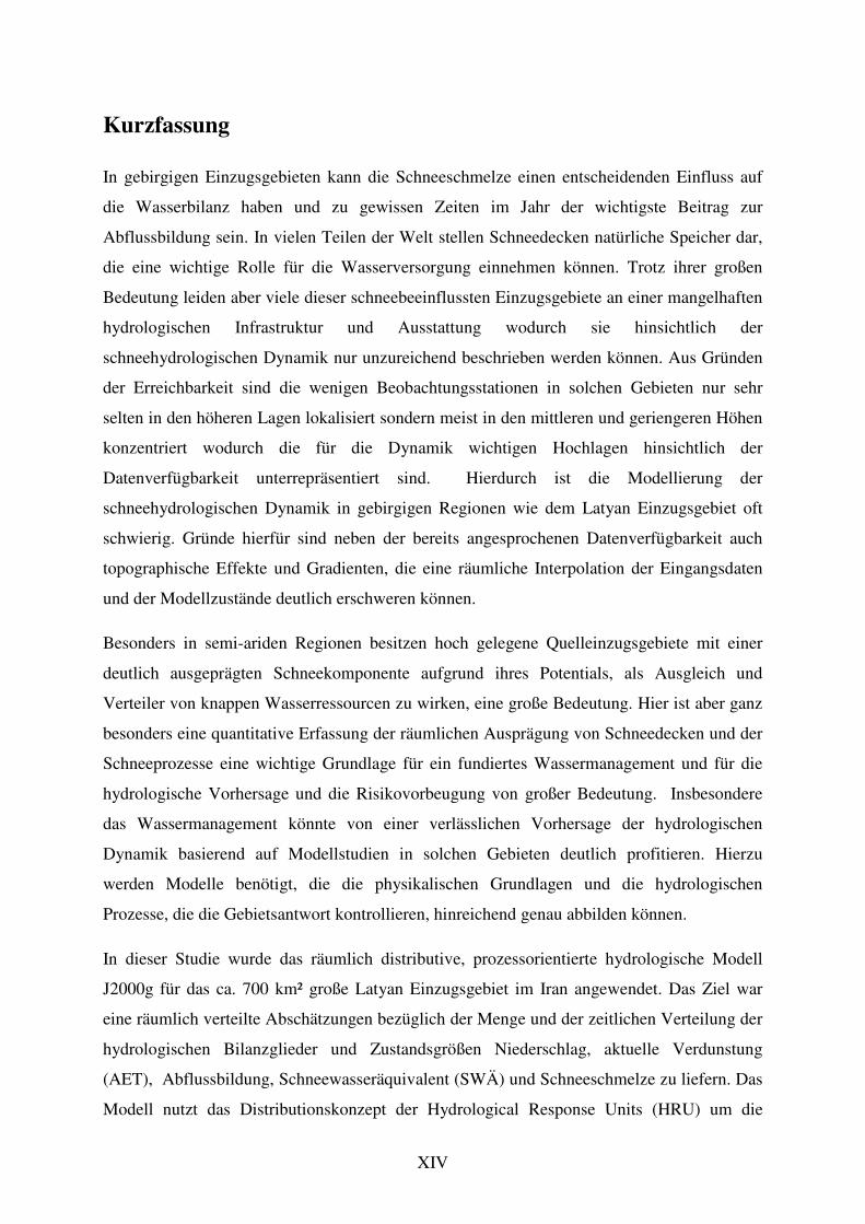
Kurzfassung
In gebirgigen Einzugsgebieten kann die Schneeschmelze einen entscheidenden Einfluss auf
die Wasserbilanz haben und zu gewissen Zeiten im Jahr der wichtigste Beitrag zur
Abflussbildung sein. In vielen Teilen der Welt stellen Schneedecken natürliche Speicher dar,
die eine wichtige Rolle für die Wasserversorgung einnehmen können. Trotz ihrer großen
Bedeutung leiden aber viele dieser schneebeeinflussten Einzugsgebiete an einer mangelhaften
hydrologischen Infrastruktur und Ausstattung wodurch sie hinsichtlich der
schneehydrologischen Dynamik nur unzureichend beschrieben werden können. Aus Gründen
der Erreichbarkeit sind die wenigen Beobachtungsstationen in solchen Gebieten nur sehr
selten in den höheren Lagen lokalisiert sondern meist in den mittleren und geriengeren Höhen
konzentriert wodurch die für die Dynamik wichtigen Hochlagen hinsichtlich der
Datenverfügbarkeit unterrepräsentiert sind. Hierdurch ist die Modellierung der
schneehydrologischen Dynamik in gebirgigen Regionen wie dem Latyan Einzugsgebiet oft
schwierig. Gründe hierfür sind neben der bereits angesprochenen Datenverfügbarkeit auch
topographische Effekte und Gradienten, die eine räumliche Interpolation der Eingangsdaten
und der Modellzustände deutlich erschweren können.
Besonders in semi-ariden Regionen besitzen hoch gelegene Quelleinzugsgebiete mit einer
deutlich ausgeprägten Schneekomponente aufgrund ihres Potentials, als Ausgleich und
Verteiler von knappen Wasserressourcen zu wirken, eine große Bedeutung. Hier ist aber ganz
besonders eine quantitative Erfassung der räumlichen Ausprägung von Schneedecken und der
Schneeprozesse eine wichtige Grundlage für ein fundiertes Wassermanagement und für die
hydrologische Vorhersage und die Risikovorbeugung von großer Bedeutung. Insbesondere
das Wassermanagement könnte von einer verlässlichen Vorhersage der hydrologischen
Dynamik basierend auf Modellstudien in solchen Gebieten deutlich profitieren. Hierzu
werden Modelle benötigt, die die physikalischen Grundlagen und die hydrologischen
Prozesse, die die Gebietsantwort kontrollieren, hinreichend genau abbilden können.
In dieser Studie wurde das räumlich distributive, prozessorientierte hydrologische Modell
J2000g für das ca. 700 km² große Latyan Einzugsgebiet im Iran angewendet. Das Ziel war
eine räumlich verteilte Abschätzungen bezüglich der Menge und der zeitlichen Verteilung der
hydrologischen Bilanzglieder und Zustandsgrößen Niederschlag, aktuelle Verdunstung
(AET), Abflussbildung, Schneewasseräquivalent (SWÄ) und Schneeschmelze zu liefern. Das
Modell nutzt das Distributionskonzept der Hydrological Response Units (HRU) um die
XV
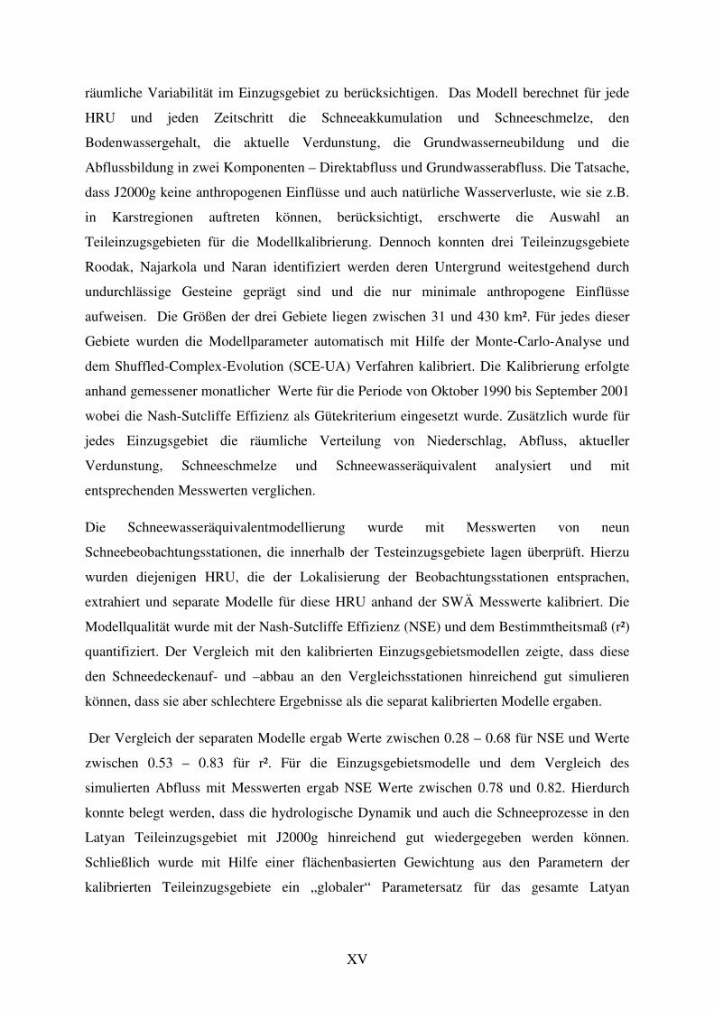
räumliche Variabilität im Einzugsgebiet zu berücksichtigen. Das Modell berechnet für jede
HRU und jeden Zeitschritt die Schneeakkumulation und Schneeschmelze, den
Bodenwassergehalt, die aktuelle Verdunstung, die Grundwasserneubildung und die
Abflussbildung in zwei Komponenten – Direktabfluss und Grundwasserabfluss. Die Tatsache,
dass J2000g keine anthropogenen Einflüsse und auch natürliche Wasserverluste, wie sie z.B.
in Karstregionen auftreten können, berücksichtigt, erschwerte die Auswahl an
Teileinzugsgebieten für die Modellkalibrierung. Dennoch konnten drei Teileinzugsgebiete
Roodak, Najarkola und Naran identifiziert werden deren Untergrund weitestgehend durch
undurchlässige Gesteine geprägt sind und die nur minimale anthropogene Einflüsse
aufweisen. Die Größen der drei Gebiete liegen zwischen 31 und 430 km². Für jedes dieser
Gebiete wurden die Modellparameter automatisch mit Hilfe der Monte-Carlo-Analyse und
dem Shuffled-Complex-Evolution (SCE-UA) Verfahren kalibriert. Die Kalibrierung erfolgte
anhand gemessener monatlicher Werte für die Periode von Oktober 1990 bis September 2001
wobei die Nash-Sutcliffe Effizienz als Gütekriterium eingesetzt wurde. Zusätzlich wurde für
jedes Einzugsgebiet die räumliche Verteilung von Niederschlag, Abfluss, aktueller
Verdunstung, Schneeschmelze und Schneewasseräquivalent analysiert und mit
entsprechenden Messwerten verglichen.
Die Schneewasseräquivalentmodellierung wurde mit Messwerten von neun
Schneebeobachtungsstationen, die innerhalb der Testeinzugsgebiete lagen überprüft. Hierzu
wurden diejenigen HRU, die der Lokalisierung der Beobachtungsstationen entsprachen,
extrahiert und separate Modelle für diese HRU anhand der SWÄ Messwerte kalibriert. Die
Modellqualität wurde mit der Nash-Sutcliffe Effizienz (NSE) und dem Bestimmtheitsmaß (r²)
quantifiziert. Der Vergleich mit den kalibrierten Einzugsgebietsmodellen zeigte, dass diese
den Schneedeckenauf- und –abbau an den Vergleichsstationen hinreichend gut simulieren
können, dass sie aber schlechtere Ergebnisse als die separat kalibrierten Modelle ergaben.
Der Vergleich der separaten Modelle ergab Werte zwischen 0.28 – 0.68 für NSE und Werte
zwischen 0.53 – 0.83 für r². Für die Einzugsgebietsmodelle und dem Vergleich des
simulierten Abfluss mit Messwerten ergab NSE Werte zwischen 0.78 und 0.82. Hierdurch
konnte belegt werden, dass die hydrologische Dynamik und auch die Schneeprozesse in den
Latyan Teileinzugsgebiet mit J2000g hinreichend gut wiedergegeben werden können.
Schließlich wurde mit Hilfe einer flächenbasierten Gewichtung aus den Parametern der
kalibrierten Teileinzugsgebiete ein „globaler“ Parametersatz für das gesamte Latyan
XVI
Einzugsgebiet erzeugt. Mit diesem Parametersatz wurden Nash-Sutcliffe Effizienzen
zwischen 0.68 und 0.79 für das Latyan Einzugsgebiet erzielt.
Es kann zusammenfassend festgestellt werden, dass die einzelnen Module und insbesondere
die Schneekomponenten des J2000g sowie das HRU Konzept für die erzielte Fragestellung
der Erfassung der hydrologischen Dynamik des Latyan Einzugsgebiet als sehr gut geeignet
betrachtet werden können. Hierdurch können mit dem Modell wichtige hydrologische
Grundlagen für eine nachhaltige Bewirtschaftung der Wasserressourcen erarbeitet werden.
1
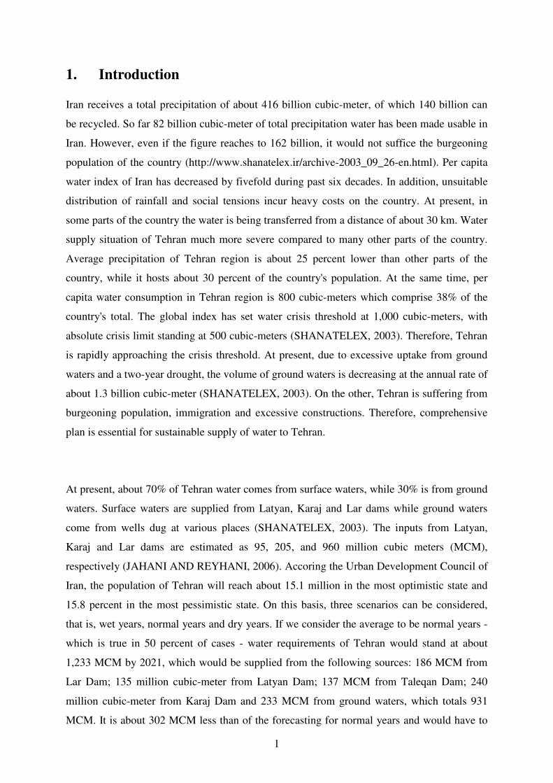
1. Introduction Iran receives a total precipitation of about 416 billion cubic-meter, of which 140 billion can
be recycled. So far 82 billion cubic-meter of total precipitation water has been made usable in
Iran. However, even if the figure reaches to 162 billion, it would not suffice the burgeoning
population of the country (http://www.shanatelex.ir/archive-2003_09_26-en.html). Per capita
water index of Iran has decreased by fivefold during past six decades. In addition, unsuitable
distribution of rainfall and social tensions incur heavy costs on the country. At present, in
some parts of the country the water is being transferred from a distance of about 30 km. Water
supply situation of Tehran much more severe compared to many other parts of the country.
Average precipitation of Tehran region is about 25 percent lower than other parts of the
country, while it hosts about 30 percent of the country's population. At the same time, per
capita water consumption in Tehran region is 800 cubic-meters which comprise 38% of the
country's total. The global index has set water crisis threshold at 1,000 cubic-meters, with
absolute crisis limit standing at 500 cubic-meters (SHANATELEX, 2003). Therefore, Tehran
is rapidly approaching the crisis threshold. At present, due to excessive uptake from ground
waters and a two-year drought, the volume of ground waters is decreasing at the annual rate of
about 1.3 billion cubic-meter (SHANATELEX, 2003). On the other, Tehran is suffering from
burgeoning population, immigration and excessive constructions. Therefore, comprehensive
plan is essential for sustainable supply of water to Tehran.
At present, about 70% of Tehran water comes from surface waters, while 30% is from ground
waters. Surface waters are supplied from Latyan, Karaj and Lar dams while ground waters
come from wells dug at various places (SHANATELEX, 2003). The inputs from Latyan,
Karaj and Lar dams are estimated as 95, 205, and 960 million cubic meters (MCM),
respectively (JAHANI AND REYHANI, 2006). Accoring the Urban Development Council of
Iran, the population of Tehran will reach about 15.1 million in the most optimistic state and
15.8 percent in the most pessimistic state. On this basis, three scenarios can be considered,
that is, wet years, normal years and dry years. If we consider the average to be normal years -
which is true in 50 percent of cases - water requirements of Tehran would stand at about
1,233 MCM by 2021, which would be supplied from the following sources: 186 MCM from
Lar Dam; 135 million cubic-meter from Latyan Dam; 137 MCM from Taleqan Dam; 240
million cubic-meter from Karaj Dam and 233 MCM from ground waters, which totals 931
MCM. It is about 302 MCM less than of the forecasting for normal years and would have to
2
reduce agricultural water supply in favour of drinking water (SHANATELEX, 2003). Scarcity
of water is a common problem especially in the urban areas of Iran because of the dry
conditions, which prevail in most of the country. There is a need for continuous drinking,
household and industrial water supply in the large cities for economic development and urban
livelihood. In addition, there can be a flooding problem in some years due to huge
precipitation. Because of these needs, it is important to manage the water resources, which
require an understanding of the hydrological processes in the catchments. This knowledge is
also required for hydrologic modelling and for transposing data from gauged catchments to
ungauged ones. Traditionally hydrological studies in Iran have been made from an
engineering point of view, whereby no or little attempt was made to relate the discharges to
the catchment characteristics (KARAMOUZ ET AL., 2001; ZARGHAAMI AND
SALAVITABAR, 2006; ZEINIVAND AND DE SMEDT, 2008).
Figure 1.1: Increasing pattern of water extraction from various catchments including the Latyan for water supply to the Tehran (Source: Zargaami and Salavitabar, 2006:P.5)
Snow accumulation and melt is an important hydrological process for the hydrological
dynamics of catchments at higher altitudes. Snowmelt is a vital source of water in many parts
of the world for public supply, hydropower, irrigated agriculture and other uses and may
significantly contribute to river floods (FERGUSON, 1999; SINGH AND SINGH, 2001;
PARAJKA ET AL., 2001). At the same time the seasonal snow cover affects also biotic
components and water quality in river basins. Distributed modelling of snow accumulation
and snowmelt is therefore an important issue. Recent advances in geographical information
3
system (GIS) and remote sensing (RS) technology allow powerful integration of GIS and RS
analytical and visualization tools with physically based hydrological models. In the field of
snowmelt modelling, such integration provides a valuable basis for better understanding of
snow accumulation and snowmelt runoff processes within the catchment, as well as for
incorporating the spatial variability of hydrological and geographical variables and their
impacts on catchment response (FERGUSON, 1999; PARAJKA ET AL., 2001). Application
and studies in terms of snow modelling by means of GIS and RS for Iranian catchments are
only sparsely available (MORID, 2004).
1.1 OBJECTIVE
One common problem that scientists encounter in developing countries is the lack of
informative data for the related study. Even if the data exist, quick on-line and timely access
to the data may be problematic and in particular the quick access to snow data, which is a
must be in operational snow melt forecasting, is not possible yet. Ground based snow
measurements are mostly gathered in form of snow courses by governmental organisations
mostly in 2-3 week periods. In such snow courses, snow water equivalent and snow depths are
measured along defined track. Most of the courses are started mainly in November or
December and they are abandoned by mid or end of March, when the snow ripens and starts
to melt, even if a reasonable amount of snow may still remain in upper mountainous areas.
For an assessment of the impact of snow processes on Iranian catchments, by the analysis of
snow pack development and the estimation of snowmelt, snow cover data as well as hydro-
meteorological parameters in the higher altitudes of the watersheds are needed. Unfortunately
such parameters are not available in the higher altitudes because precipitation and temperature
data are generally measured in the lower or moderate altitudes of the catchments only.
Because of this lack of data only very few studies using models are available for the area of
interest. The number of snowmelt models which was applied in various catchments in the Iran
is limited to the snow runoff model (SRM) which was used in the very rare simulation of
snowmelt runoff in Iranian mountainous catchments. To overcome that lack of data and to
enforce modelling activities in such data remote areas globally available data sets from
regionalization, using Hydrological Response Units approach as well as RS availability like
Shuttle Radar Topography Mission SRTM for Digital Elevation Model (DEM) could be
available. To make most out use such data it should be used as drivers for hydrological
models to allow a simulation of the complex processes and hereby a quantification of the
hydrological dynamics.
4
Therefore, the main objective of the present study is Develop better understanding of
hydrological process interaction in Iranian catchments by means of GIS and process-oriented
modelling
The detail objectives of the research are:
• Providing scientific basis for sustainable water resource management in the Latyan
catchment
- To analyze the hydro-meteorological data in terms of areal extent, frequencies and
intensities
- Delineation of Hydrological Response Units (HRUs) using GIS and RS
• Improvement of the understanding of snow driven hydrological dynamics in the
Latyan catchment
- Spatial distributed hydrological modelling of snow driven catchments using J2000g
5
2. Research Review
6
Snow is an important component of the hydrological cycle. A reasonable snowmelt estimate
is essential for the regional planning of water resources. To achieve this objective, data such
as the snow cover, snow depth, and water equivalent are necessary. Snow cover is an
important index for predicting the spring melt, and it is interpreted better than the other snow
parameters. Snowpack are the drinking water source for many communities. Snowpack are
also studied in relation to climate change and global warming. Snowpack modelling is done
for flood forecasting, water resource management, and climate studies.
In hydrology, snowmelt is surface runoff produced from melting snow. It can also be used to
describe the period or season during which such runoff is produced. Water produced by
snowmelt is an important part of the annual water cycle in many parts of the world and in
some cases contributing high fractions of the annual runoff in a watershed. Predicting
snowmelt runoff from a drainage basin can be a part of designing water control projects.
Recent development in snow hydrology has continued to emphasize the temporal and spatial
variability in snow sublimation and melt and, therefore, the spatial heterogeneity in surface
energy fluxes. There is also a rising interest in modelling snow hydrology and snow ecology
(WOO and MARSH, 2005).
2.1 Snow in the hydrological cycle
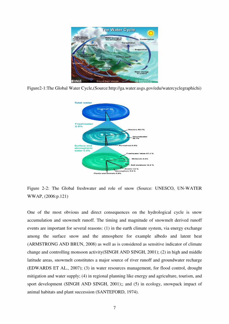
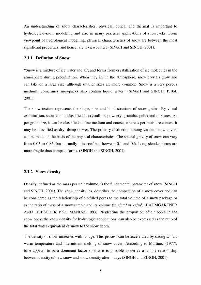
The global water cycle is the process by which our freshwater is produced and as illustrated in
figures 2-1 and 2-2, snow has a big role in this process as a vital source of produce freshwater.
Only 1.74 % of the world total water storages which accounts for 68.7 % of the fresh water
reserves (SEIDEL AND MARTINEC, 2004:P. 5) are stored as snowpack. Snow plays a vital
role in distributing the natural water resource.
7
Figure2-1:The Global Water Cycle,(Source:http://ga.water.usgs.gov/edu/watercyclegraphichi)
Figure 2-2: The Global freshwater and role of snow (Source: UNESCO, UN-WATER
WWAP, (2006:p.121)
One of the most obvious and direct consequences on the hydrological cycle is snow
accumulation and snowmelt runoff. The timing and magnitude of snowmelt derived runoff
events are important for several reasons: (1) in the earth climate system, via energy exchange
among the surface snow and the atmosphere for example albedo and latent heat
(ARMSTRONG AND BRUN, 2008) as well as is considered as sensitive indicator of climate
change and controlling monsoon activity(SINGH AND SINGH, 2001); (2) in high and middle
latitude areas, snowmelt constitutes a major source of river runoff and groundwater recharge
(EDWARDS ET AL., 2007); (3) in water resources management, for flood control, drought
mitigation and water supply; (4) in regional planning like energy and agriculture, tourism, and
sport development (SINGH AND SINGH, 2001);; and (5) in ecology, snowpack impact of
animal habitats and plant succession (SANTEFORD, 1974).
8
An understanding of snow characteristics, physical, optical and thermal is important to
hydrological-snow modelling and also in many practical applications of snowpacks. From
viewpoint of hydrological modelling, physical characteristics of snow are between the most
significant properties, and hence, are reviewed here (SINGH and SINGH, 2001).
2.1.1 Defintion of Snow
“Snow is a mixture of ice water and air; and forms from crystallization of ice molecules in the
atmosphere during precipitation. When they are in the atmosphere, snow crystals grow and
can take on a large size, although smaller sizes are more common. Snow is a very porous
medium. Sometimes snowpacks also contain liquid water” (SINGH and SINGH: P.104,
2001).
The snow texture represents the shape, size and bond structure of snow grains. By visual
examination, snow can be classified as crystalline, powdery, granular, pellet and mixtures. As
per grain size, it can be classified as fine medium and coarse, whereas per moisture content it
may be classified as dry, damp or wet. The primary distinction among various snow covers
can be made on the basis of the physical characteristics. The special gravity of snow can vary
from 0.05 to 0.85, but normally it is confined between 0.1 and 0.6. Long slender forms are
more fragile than compact forms. (SINGH and SINGH, 2001)
2.1.2 Snow density
Density, defined as the mass per unit volume, is the fundamental parameter of snow (SINGH
and SINGH, 2001). The snow density, ρs, describes the compaction of a snow cover and can
be considered as the relationship of air-filled pores to the total volume of a snow package or
as the ratio of mass of a snow sample and its volume (in g/cm³ or kg/m³) (BAUMGARTNER
AND LIEBSCHER 1996; MANIAK 1993). Neglecting the proportion of air pores in the
snow body, the snow density for hydrologic applications, can also be expressed as the ratio of
the total water equivalent of snow to the snow depth.
The density of snow increases with its age. This process can be accelerated by strong winds,
warm temperature and intermittent melting of snow cover. According to Martinec (1977),
time appears to be a dominant factor so that it is possible to derive a simple relationship
between density of new snow and snow density after n days (SINGH and SINGH, 2001).
9
ρn= ρ0 (n + 1)º·³ Equation 2-1
Where, ρ0 is the average density of new snow (0.1 gm/cc) and ρn is the snow density after n
days. Or,
ρs = HS / HWE [cm] Equation 2-2
Where, ρs is the snow density, HS is the Height snow and HWE is height or snow water
equivalent.
When the deposition of snow crystals begins their transformation, dynamic process of
compaction and metamorphism of the snow takes place (RANGO ET AL., 1996a/b).
Accordingly, in many studies and model approaches, the initial density of snowfall
dynamically modified by the density of snow during the snow period differed (BRAUN 1985;
VEHVILÄINEN 1992; GRAY AND PROWSE 1993; RANGO AND MARTINEC 1995;
BAUMGARTNER AND LIEBSCHER 1996).
The initials snow density e.g. depends on a number of climatic factors during the deposit such
as air temperature, humidity or wind speed. So, it can be assumed that wet snow deposits,
which developed at temperatures around the freezing point, are set higher snow densities than
cold dry deposits (COLBECK ET AL., 1990). KUCHMENT et al. (1983) derived initial snow
density as a function of air temperature. He found an exponential relationship between the
increase of temperature and snow density. Due to the high variability and complexity of the
factors of influence in some snow-hydrological modelling approaches, the initials snow
density is accepted an average value of 0.1 g/cm³ for simplification (MARTINEC AND
RANGO, 1991).
In the further process of the snowpack formation, strong compaction processes that are
complex meteorological, seasonal and local contexts can be determined (BRAUN 1985;
ROHRER 1992; NAKAWO AND HAYAKAWA 1998). DINGMAN (1994) reported a
strong relationship between snow compaction and wind. On the other hand, BRAUN (1985)
found no clear causal relationship between the snow density and individual factors such as
elevation or snow depth.
On the basis of the wide range of variation for observed snow density values between deposit
and ablation, a high variability of snow density has been described in the literature. BRAUN
(1985) found a variation ranges from 0.1-0.4 g/cm ³ for 50 cm snow cover. MANIAK (1993)
10
indicated a density of 0.05-0.13 g/cm ³ for new powder snow. For granular powder snow
(0.25 g/cm³) and granular snow (0.33-0.4 g/cm³), he found an increase in snow density (0.5-
0.6 g/cm³). Furthermore, BAUMGARTNER AND LIEBSCHER (1996) found that new snow
which depends upon humidity and packing condition, can exhibit densities between 0.01 and
0.2 g/cm ³. They identified first depletion product of new snow as snowfall with densities
between 0.15 and 0.25 g/cm³. With the passage of time, ongoing transformation of snow
structure by grain melting or regulation processes leads to the development of old snow,
which exhibits densities up to 0.6 g/cm³. DUNN AND COLOHAN (1999) quoted various
empirical investigations. According to him, the density of fresh snow already lies between
0.05 and 0.3 g/cm³. In case of a gradual compaction, it lies between 0.3 and 0.7 g/cm³for older
snow deposits.
2.1.3 Snow depth
The snow depth or snow cover thickness means the vertical height of a snow cover
(BAUMGARTNER AND LIEBSCHER 1996). It is recorded also in standard measuring
programs regularly in cm (International Commission on Snow and Ice (ICSI)-classification,
NAKAWO/HAYAKAWA 1998). Snow depth is considered as snow-hydrologic size, which
varies like the other physical characteristics and can be detected easily in dependence of
different climatic, topographic and vegetative factors which influence strongly in space and
time. Generally, snow precipitation ensures for an increase, and evaporation and melts causes
a dynamic reduction of the snow height during compaction processes. The snow depth, HS,
must be understood as secondary size and can be determined by the relationship of snow
water equivalent (HWE) and snow density (ρs) (DINGMAN, 1994; BAUMGARTNER AND
LIEBSCHER, 1996):
HS = ρs / HWE [cm] Equation 2-3
2.2 Snow water equivalent (SWE)
The snow water equivalent, SWE, is considered to be the most important hydrological snow-
related variable. It is defined as the snow cover both in solid and liquid form, containing a
11
certain quantity of water, measured in mm, L/m² or kg/m². Alternatively, SWE is defined as
the vertical depth of water which is obtained by the melting of snow (WOHLRAB ET AL.,
1992; BAUMGARTNER AND LIEBSCHER, 1996; SINGH and SINGH, 2001).
According to Singh and Singh (2001) the water equivalent of a snow cover, HSW, of
thickness D is given by:
1
n
i i
i
HSW d Dρ ρ=
= =∑ Equation 2-4
Where the snow cover of thickness D has been divided in to n homogeneous thicknesses d1,
d2… dn having densities ρ1, ρ2… ρn, respectively, and ρ is mean density of snow cover and
may be defined by the following relation:
1
1/n
i i
i
D dρ ρ=
= ∑ Equation 2-5
The amount of snow water equivalent varies greatly, depending on various regional and local
factors. A linear empirical relationship between the increase of the terrain and the height of
the water equivalent has been indicated (MARTINEC 1991). Martinec (1991) found no more
increase in snow water equivalent above 2800 meter above see level (m.a.s.l) elevation. If the
influence of the terrain elevation is described as dominant, other regional factors such as the
latitude, topography and vegetation does not affect much. Thus, the influence of high dense
forest particularly with the snow floor system proves as strongly reducing factor for the height
of the water equivalent. In contrast, the exposure strengthened during the ablation by
modifying melt rates on the development of water-equivalent (ISHII AND FUKUSHIMA,
1994).
In the standard measurement programs, the water equivalent is rarely determined. Generally,
in the European stations, point measurements are error-prone values. So, regionalization is
required to obtain best possible values (MARTINEC AND RANGO, 1981). In the USA, the
12
snow telemetry (SNOTEL) network is used for determining snow water equivalent
(SIMPSON ET AL., 1998; FERGUSON, 1999). Based upon recent remote sensing and radar
techniques, it is possible to obtain spatial images of the water equivalent (MARTINEC ET
AL., 1991; LUNDBERG AND THUNEHED, 2000). With the help of passive microwave
data for terrain, water equivalent can be calculated. However, Rango et al., (1996a/b)
described that the assessment of values are somewhat negated by the variability of size and
shape of snow crystals. Depending on the recording technology, the thin and waterlogged
snow is expected to be falsely measured, as reflections of the underlying soil surface and high
liquid water contents in the snow provide distortion (LUNDBERG AND THUNEHED,
2000). Also, forest areas provide distortion of the recorded signals (FERGUSON 1999).
Moreover, image resolution, surface cover and frequency recording of most remote sensing
techniques are still very limited (BRAUN 1985; BLÖSCHL AND KINBAUER, 1992;
NAKAWO AND HAYAKAWA, 1998). However, an exception is made regarding the
resolution from active microwaves, which are not able to detect the water equivalent of dry
snow cover (FERGUSON, 1999).
Frequently, the snow water equivalent is calculated from the measured rainfall depth. Besides,
a simple mass relationship between snow water equivalent, snow density and snow height can
be set up. In many investigations and applications of models to derive and describe the snow
storage variable, water equivalent is used (VEHVILÄINEN, 1992; WOHLRAB ET AL.,
1992; DINGMAN, 1994; MARTINEC, ET AL., 1994b). This relationship is as follows:
HWE= HS * ρs [mm] Equation 2-6
Where, HWE is height or snow water equivalent [mm], HS is snow depth [cm], and ρs is
snow density [g / cm³].
2.3 Snowmelt
The snowmelt process is defined as the phase transition of solid snow ingredients parts (ice
crystals, Ice grains) into liquid water, for which about 340 joules per gram (j/g) of energy are
needed. Snowmelt processes is determined by the energy balance of the snowpack. The
13
energy balance of the snow is predominantly determined by atmospheric and microclimatic
variables (BAUMGARTNER AND LIEBSCHER, 1996). The necessary energy quantity, in
order to raise the snow temperature to the melting point, corresponds to the cooling content of
snow pack. After reaching isothermal conditions within the regarded snow pack at 0°C, each
further energy input causes melt. The two primary factors of the energy balance for using melt
are the short-wave net radiation and the perceptible heat flow (KUHN 1984; RACHNER
AND MATTHÄUS, 1986; DINGMAN, 1994; RACHNER ET AL., 1997).
The respective importance of the individual energy components for the melt is a function of
weather processes (BLÖSCHL ET AL., 1987). For instance, with open land snow covers in
the alpine and polar areas, the sun light is considered as main influencing factor for melting
processes. Higher influence of sun increases the further melting process in the spring
(BRAUN 1985). According to Baumgartner and Liebscher (1996) the radiation supplies
approximately 80 percent of the melting energy for mountain snow covers. However, in
lowland snow covers, where often wet weather conditions predominate, 50 percent of the heat
of melting comes out from perceptible and latent heat flows. Rachner et al. (1997)
emphasized the importance of heat transfer of flowing air for melting mountain snow covers
because of heat transport by moisture exchange. On the other hand, turbulent heat flows as a
function of the wind speed. Generally, in the lowlands and the low mountain area, high air
temperatures, high humidity and strong wind is considered as crucial determinants of melting
processes aforementioned (HERRMANN AND RAU, 1984; KUHN, 1984; BLÖSCHL ET
AL., 1987; BAUMGARTNER AND LIEBSCHER, 1996).
Due to the storage capability of snow for liquid water, the snowmelt rate and water loss rate
from snow cover are not particularly identical at the beginning of a melting period. If the
retention capacity of the snowpack for liquid water is exceeded, melt water percolated by the
snowpack occurs only at the base of the snowpack (FERGUSON, 1986; BLÖSCHL AND
KIRNBAUER, 1992; SINGH ET AL., 1998; KATTELMANN, 1998).
Over logging related crystal transformations in forest areas and compactions, the dynamic
melting process itself induced a sustained increase in melting of snowpack. Besides water-
saturated snow covers in recent melt or rain entry, a direct translation of the stored liquid
water leads to direct discharges from snowpack (FERGUSON, 1986; SINGH ET AL., 1998).
Accordingly, the condition of the snow package at the time of entering melting conditions
from snowpack is of crucial importance for causing melt and the water discharge (RACHNER
AND MATTHÄUS 1984; RANGO AND MARTINEC 1995; SINGH ET AL., 1998).
14
2.3.1 Effect of rainfall, topography and landcover on snowmelt
Depending on the amount, intensity and duration of the precipitation, snow cover thickness
and snowpack logging will significantly increase the melting process. On thin snow cover,
moderate rainfall can contribute to complete-melt (KUUSISTO, 1980; BAUMGARTNER
AND LIEBSCHER 1996; SINGH ET AL., 1998).
Singh et al., (1998) emphasized that the melting snow and runoff response of snowpack due to
heavy rain is significantly higher than melt alone. Thus, in particular, the destructuring effect
and registered transmitted rainwater have high importance for the melting and release of water
attached. Especially, in areas with variable winter conditions, various authors described the
influence of rain as the most important determinant of ablation process (KUUSISTO, 1980;
WOHLRAB ET AL., 1992; RACHNER ET AL., 1997). In contrast, the energetic
contribution of rain to melt described as very low (BAUMGARTNER AND LIEBSCHER
1996; SINGH ET AL., 1998).
The snow cover depletion also varies spatially and temporally depending on the level terrain,
the slope exposure, tilt, and the forest area. As the name of the location factors influence is
very specific and variable, only qualitative statements can be made. On the contrary,
generalized quantification of the degree of influence is not possible (HERRMANN AND
RAU, 1984; BRAUN, 1985; BLÖSCHL AND KIRNBAUER, 1992; ISHII AND
FUKUSHIMA, 1994; BAUMGARTNER AND LIEBSCHER, 1996; RACHNER ET AL.,
1997; KATTELMANN, 1998).
The influence of the ground level can be explained mainly by the decrease in temperature and
increase of radiation energy with increasing altitude, as well as the prevailing weather
conditions (BAUMGARTNER AND LIEBSCHER, 1996; RACHNER ET AL., 1997).
Generally, powerful radiation dominated melting snow in high mountain passes gradually.
However, it often comes in lower layers by turbulent weather conditions rapidly due to
ablation of the most thin snow covers (HERRMANN AND RAU 1984; BAUMGARTNER
AND LIEBSCHER, 1996).
The importance of slope and exposure in melting process can be felt especially in radiative
weather conditions, where north-facing slopes received significantly lower energy than south-
15
facing slopes. Accordingly, it resulted in delayed melting in northern side and accelerated
melting in the southern side (BRAUN, 1985; BLÖSCHL AND KIRNBAUER, 1992).
Depending on the density of the canopy, most of the evergreen forest may be expected to have
reduced and delayed melt as compare to open areas. In contrast, winter bare deciduous forest
is not significantly different from open areas in terms of melt. Often, reduction in melting
takes place by the already smaller accumulation of snow, for example, due to high
interception values and higher evaporation losses under forest. Melting delays are mainly due
to shading effects of the crowns, the days of radiation, if the melt is mainly due to sun
exposure, are effective. In addition, lower melt rates may be caused by the attenuation of wind
speeds, which resulted in reduction of turbulent heat exchange (DICKISON ET AL., 1984;
BUTTLE AND MCDONNELL, 1987; ISHII AND FUKUSHIMA, 1994; BENGTSSON
AND SINGH, 2000).
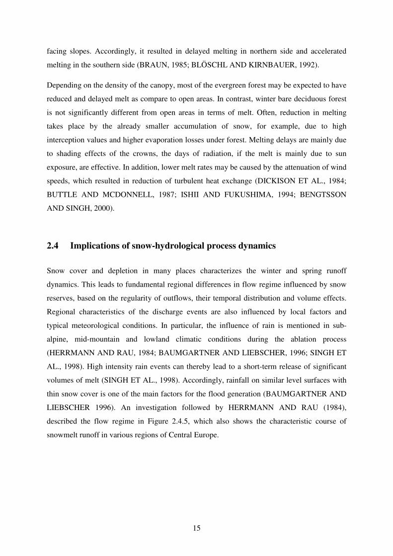
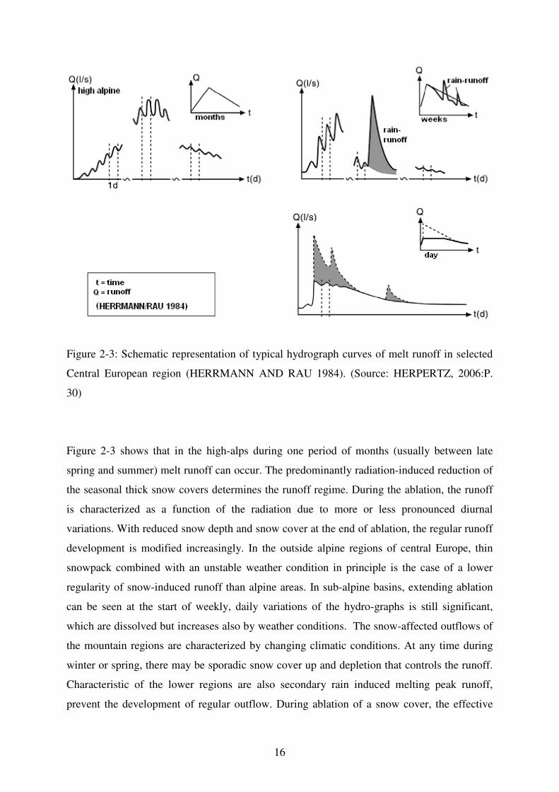
2.4 Implications of snow-hydrological process dynamics
Snow cover and depletion in many places characterizes the winter and spring runoff
dynamics. This leads to fundamental regional differences in flow regime influenced by snow
reserves, based on the regularity of outflows, their temporal distribution and volume effects.
Regional characteristics of the discharge events are also influenced by local factors and
typical meteorological conditions. In particular, the influence of rain is mentioned in sub-
alpine, mid-mountain and lowland climatic conditions during the ablation process
(HERRMANN AND RAU, 1984; BAUMGARTNER AND LIEBSCHER, 1996; SINGH ET
AL., 1998). High intensity rain events can thereby lead to a short-term release of significant
volumes of melt (SINGH ET AL., 1998). Accordingly, rainfall on similar level surfaces with
thin snow cover is one of the main factors for the flood generation (BAUMGARTNER AND
LIEBSCHER 1996). An investigation followed by HERRMANN AND RAU (1984),
described the flow regime in Figure 2.4.5, which also shows the characteristic course of
snowmelt runoff in various regions of Central Europe.
16
Figure 2-3: Schematic representation of typical hydrograph curves of melt runoff in selected
Central European region (HERRMANN AND RAU 1984). (Source: HERPERTZ, 2006:P.
30)
Figure 2-3 shows that in the high-alps during one period of months (usually between late
spring and summer) melt runoff can occur. The predominantly radiation-induced reduction of
the seasonal thick snow covers determines the runoff regime. During the ablation, the runoff
is characterized as a function of the radiation due to more or less pronounced diurnal
variations. With reduced snow depth and snow cover at the end of ablation, the regular runoff
development is modified increasingly. In the outside alpine regions of central Europe, thin
snowpack combined with an unstable weather condition in principle is the case of a lower
regularity of snow-induced runoff than alpine areas. In sub-alpine basins, extending ablation
can be seen at the start of weekly, daily variations of the hydro-graphs is still significant,
which are dissolved but increases also by weather conditions. The snow-affected outflows of
the mountain regions are characterized by changing climatic conditions. At any time during
winter or spring, there may be sporadic snow cover up and depletion that controls the runoff.
Characteristic of the lower regions are also secondary rain induced melting peak runoff,
prevent the development of regular outflow. During ablation of a snow cover, the effective
17
runoff extends only for a period of days (HERRMANN AND RAU, 1984; BAUMGARTNER
AND LIEBSCHER 1996)
2.5 Snow modelling
Core of snow-hydrological modelling approaches is simulation of snowmelt. The main
processes in snow accumulation and ablation models are: accumulation of new snow, snow
settlement, snowmelt caused by heat transfer from air and rain, water holding capacity,
refreezing of water in the snow pack, temperature changes of snow, and water percolation
through snow. There are two fundamental approaches of snow modelling: the energy balance
method and the temperature index method (TURČAN, 1990).
The energy balance method simulates the physical processes that affect the thermal energy
content of the snow pack such as sensible, latent and ground heat fluxes, heat conduction
between layers, and energy released from phase changes. This type of model requires a
number of inputs including incoming and reflected solar radiation, incoming long wave
radiation, temperature, precipitation, relative humidity, and wind. Normally, data for
determination of long-wave and short-wave radiation balance as well as sensible and latent
heat flows are needed. Because of their nature, physically-based models typically require less
calibration because their parameters are assumed to represent measurable characteristics.
These data are available but limited. As a result, relatively insignificant elements of the
balance are neglected and more important factors like net short wave radiation and albedo as
their determinant are either measured or derived. FERGUSON, (1999) described the
extrapolation of this estimation to be very error-prone. Moreover, BLÖSCHL, (1991)
indicated that temporal and spatial albedo variation strongly varies and is difficult to estimate.
He also described a high sensitivity of the most energy balance procedures for the albedo,
which can lead to much larger misidentifications of the melting volume, for example,
inaccuracies in estimating the air temperature. FERGUSON, (1999) focussed on the high
variability of the particular balance in terms of temporal (daily, seasonal and synoptic scale)
and spatial attributes.
In particular, the energy model approaches usually need very high data, but in the applied
hydrology, preferred temperature index or degree-day factor methods can be used to simulate