Conference Paper, Published Version

Hieu, Mai Trung; Nowak, Wolfgang; Kopmann, RebekkaUsing algorithmic differentiation for uncertainty analysisZur Verfügung gestellt in Kooperation mit/Provided in Cooperation with:TELEMAC-MASCARET Core Group

Verfügbar unter/Available at: https://hdl.handle.net/20.500.11970/104343

Vorgeschlagene Zitierweise/Suggested citation:Hieu, Mai Trung; Nowak, Wolfgang; Kopmann, Rebekka (2015): Using algorithmicdifferentiation for uncertainty analysis. In: Moulinec, Charles; Emerson, David (Hg.):Proceedings of the XXII TELEMAC-MASCARET Technical User Conference October 15-16,2046. Warrington: STFC Daresbury Laboratory. S. 52-58.

Standardnutzungsbedingungen/Terms of Use:

Die Dokumente in HENRY stehen unter der Creative Commons Lizenz CC BY 4.0, sofern keine abweichendenNutzungsbedingungen getroffen wurden. Damit ist sowohl die kommerzielle Nutzung als auch das Teilen, dieWeiterbearbeitung und Speicherung erlaubt. Das Verwenden und das Bearbeiten stehen unter der Bedingung derNamensnennung. Im Einzelfall kann eine restriktivere Lizenz gelten; dann gelten abweichend von den obigenNutzungsbedingungen die in der dort genannten Lizenz gewährten Nutzungsrechte.

Documents in HENRY are made available under the Creative Commons License CC BY 4.0, if no other license isapplicable. Under CC BY 4.0 commercial use and sharing, remixing, transforming, and building upon the materialof the work is permitted. In some cases a different, more restrictive license may apply; if applicable the terms ofthe restrictive license will be binding.

Using algorithmic differentiation for uncertainty analysis

Mai Trung Hieu, Wolfgang Nowak University of Stuttgart

IWS/LS3 - Pfaffenwaldring 5a Stuttgart, Germany

mai.trunghieu.vn@gmail.com Wolfgang.nowak@iws.uni-stuttgart.de

Rebekka Kopmann Bundesanstalt für Wasserbau

BAW - Kußmaulstr. 17 Karlsruhe, Germany

rebekka.kopmann@baw.de

Abstract— Although numerical modelling is state of the art and

has been very helpful in river engineering for a long time, it

should not be neglected that uncertainties are unavoidable in

numerical modelling. Uncertainty analysis can help to identify

which model parameters cause the largest share of overall simu-

lation uncertainty, and to find the locations and time periods or

system states that are subject to the largest predictive uncertain-

ties. Three methods for uncertainty analysis of numerical simula-

tions with TELEMAC-2D have been used and compared: The

Monte Carlo method (MC), the First-Order Second Moment

method based on numerical differentiation (FOSM/ND) and the

same based on algorithmic differentiation (FOSM/AD). The

methods have been compared on an application to a laboratory

experiment with groynes. With an in-situ application of the un-

certainty methods to a 10 km long stretch of River Rhine be-

tween Neuss and Düsseldorf, the practical applicability in river

engineering could be shown.

I. INTRODUTION

Numerical modelling is state of the art and has proven very helpful in river engineering. However, numerical modelling is subject to inevitable sources of uncertainty such as deficient descriptions of physical processes, estimated initial/boundary conditions and uncertain model parameters. The latter are un-certain due to measurement errors, natural variability or due to unsatisfactory parameterization. These sources of uncertainty may have serious influence on simulation results and subse-quent engineering decisions. Therefore, it is necessary to quan-tify the resulting uncertainty of model results in order to ap-praise their reliability. Uncertainty analysis reveals the loca-tions and time periods or system states that are subject to the largest predictive uncertainties. Furthermore, it can identify the model parameters causing the largest share of overall simula-tion uncertainty. So-called sensitivities can be used to describe the influence of uncertain parameters to model predictions, and can guide efforts of model refinement or data collection.

This study applies and compares three methods for uncer-tainty analysis of TELEMAC/2D simulations: The Monte Carlo method (MC) and the First-Order Second Moment meth-od with numerical differentiation (FOSM/ND) and with algo-rithmic differentiation (FOSM/AD). The application scenarios are a laboratory experiment with groynes and a 10 km stretch of River Rhine between Neuss and Düsseldorf.

MC is a very general uncertainty quantification tool that re-quires no assumptions on linearity of the parameter-to-prediction relations in models and poses no restrictions on allowable probability distributions of input parameters. How-ever, MC requires a huge number of model runs for statistically robust uncertainty estimates. In waterways engineering, a typi-cal single model run can take days or weeks even in modern parallel computing environments. Therefore, MC is only par-tially feasible for real-world projects.

It is well known that FOSM methods can be much faster than MC, as we will illustrate in Section III/A. Thus, they are better applicable to real-world problems. However, for FOSM the parameter-prediction relations in models must be linear (or at most weakly non-linear) due to the first-order approxima-tions taken. Additionally, FOSM can provide probability dis-tributions of model output only if all uncertain model inputs follow Gaussian distributions.

FOSM/ND calculates the sensitivities required for the first-order approximation numerically using finite differences. Therefore, the number of required model runs is the number of uncertain parameters plus one (simple differences) or two times the number of parameters plus one (central differences for better precision).

In FOSM/AD, the sensitivities are computed based on so-called adjoint states or related concepts, which require simula-tion runs with a modified numerical model. The required modi-fied model is obtained through a special AD compiler for algo-rithmic differentiation. Thus, FOSM/AD avoids numerical differentiation and yields sensitivities accurate to machine precision (more accurate than central differences) with a num-ber of modified model runs equal to only the number of uncer-tain parameters. One model run with the AD compiler is nearly 2 times slower than a normal model run, so that AD provides more accurate sensitivities than ND in less computing time than central differences.

In section II, a short introduction to the used uncertainty analysis methods is given. Section III presents two applications of the uncertainty methods, featuring simulations of a laborato-ry experiment for comparing the methods, and simulations of a 10 km long stretch of River Rhine for showing the engineering relevance of uncertainty analysis. Section IV provides discus-sion and conclusions.

22nd Telemac & Mascaret User Club STFC Daresbury Laboratory, UK, 13-16 October, 2015

II. UNCERTAINTY ANALYSIS METHODS

Three methods were applied for analysing the uncertainty due to uncertain input parameters of two TELEMAC-2D mod-els: The well-known Monte-Carlo method and the First-Order Second Moment method based on numerical differentiation or based on algorithmic differentiation. With all methods, the influence of uncertain input parameters to the output variables could be investigated.

A. Monte-Carlo Method (MC)

Following the MC principle, a large number N of randomly generated input values for all uncertain input parameters pi are generated according to their (joint) probability distributions. For each of these sets of input values, simulation runs must be conducted. The results are analysed statistically to obtain mean values, variances, probability distributions and confidence intervals for all output variables of interest. The latter include in our case the water depth Hk=H(xk,pi), which depends on the uncertain input parameters pi. The variance, for example, is approximated by MC as:

𝑉𝑎𝑟 𝐻 ≃ 𝐻 𝑝 − 𝐻 (1)

For this study, N=1000 simulation runs were assumed to be sufficient. There exist some techniques to reduce the number of model runs while preserving the same accuracy (e.g. Latin Hypercube Sampling [1], Monte Carlo CL method [2], meta modelling [3]), but they are not taken into account here. In all these improved techniques, the approximation error of the statistical analysis remains proportional to the square root of N, which is typical for all sampling-based uncertainty analysis methods like MC.

B. First-Order Second Moment method (FOSM)

FOSM is an adequate method for linear or slightly non-linear problems with assumed Gaussian distributions for the uncertain parameters as well as for the output variables. Apply-ing a Taylor expansion for the output variables Hk=H(xk,pi), FOSM approximates their variance as

𝑉𝑎𝑟 𝐻 ≃ ⋅ 𝐶𝑜𝑣 𝑝 ⋅ (2)

where 𝜕𝐻 𝜕𝑝 is the vector of partial derivatives (“sensi-tivitiy”) of 𝐻 with respect to all parameters 𝑝 . The covariance matrix 𝐶𝑜𝑣 𝑝 between all uncertain parameters has to be chosen from measurements or literature values. When assum-ing that 𝑝 are not correlated, the variance simplifies to:

𝑉𝑎𝑟 𝐻 ≃   ⋅ 𝜎 (3)

where 𝜎 is the variance of parameter 𝑝 . Based on the Gaussian assumption, confidence intervals for the output vari-ables can be derived. For example, the 95% confidence interval is the mean value plus/minus two times the standard deviation.

FOSM with numerical differentiation (FOSM/ND)

The sensitivities 𝜕𝐻 𝜕𝑝 can be calculated numerically with finite differences. For central differences, two simulation runs, e.g., with 𝑝 ± 𝜎 for each uncertain parameter are needed. Only if the parameter-to-prediction relation is linear, there is no effect of different values of 𝜎 . For strongly non-linear functions, the choice of a proper parameter difference between the two simulation runs becomes essential to get the useful local derivatives.

FOSM with algorithmic differentiation (FOSM/AD)

Algorithmic differentiation (AD) is a method for compu-ting derivatives of functions implemented as numerical simula-tion programs in a semi-automatic manner. Often, only mini-mal manual adaption of the computing code is needed. New model versions can be differentiated easily by reapplying the compiler. Here, the so-called tangent-linear or forward mode of AD is used. For our case, this is more efficient than the adjoint mode as the number of uncertain input variables is relatively small compared to the number of output variables. Further information about AD methods can be found elsewhere (e.g., [4], [5], www.autodiff.org). A tangent-linear version of TELEMAC-2D and SISPYHE [6] has been created with the AD-enabled NAG Fortran compiler [7].

Using an AD version of TELEMAC-2D, the sensitivities 𝜕𝐻 𝜕𝑝 can be calculated directly and up to machine preci-sion. For each uncertain parameter, one simulation run with the AD code is needed.

III. APPLICATIONS

We use two application cases for comparing the three methods. A first comparison between the three methods has been done with a fast simulation model for the laboratory ex-periment Schönberg (see Section III/A). The second applica-tion is based on simulations of an actual river stretch of River Rhine (see Section III/B) and demonstrates exemplarily the possibilities of uncertainty analysis for numerical simulations in river engineering.

A. Schönberg model

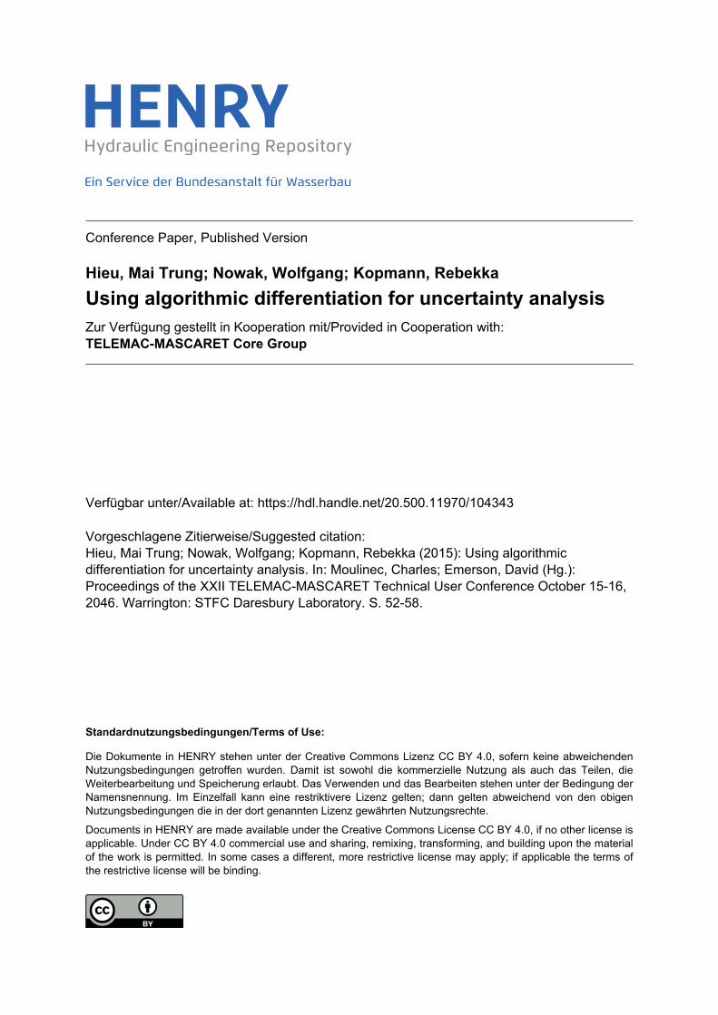
The laboratory model Schönberg (see figure 1) was con-ducted at BAW for groyne investigations in the project “eco-logical optimisation of groynes in River Elbe” [8]. The model geometry was oriented at the stretch of River Elbe near Schön-berg (El-km 439.3 – 446), which is representative for the lower Middle Elbe. The numerical model we use was built up in that project [9]. Due to the slight bend and the groynes, the flow characteristic is adequately complex as in natural rivers. The experimental setup is relatively small (about 30 m long and 9 m wide). As the numerical model was built with a triangular mesh of 5127 nodes and 10179 elements and executed in paral-lel mode on 32 cores, the simulations ran sufficiently fast for in-depth comparison of the three uncertainty quantification methods.

22nd Telemac & Mascaret User Club STFC Daresbury Laboratory, UK, 13-16 October, 2015

Figure 1. Laboratory model Schönberg

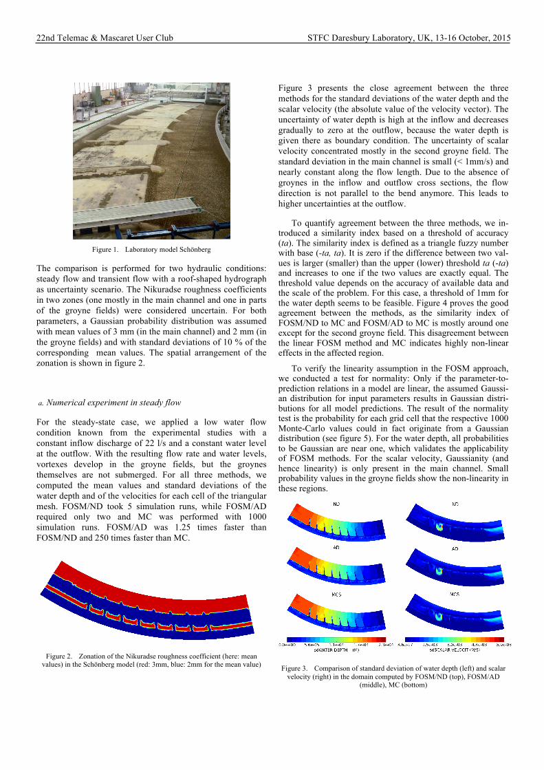
The comparison is performed for two hydraulic conditions: steady flow and transient flow with a roof-shaped hydrograph as uncertainty scenario. The Nikuradse roughness coefficients in two zones (one mostly in the main channel and one in parts of the groyne fields) were considered uncertain. For both parameters, a Gaussian probability distribution was assumed with mean values of 3 mm (in the main channel) and 2 mm (in the groyne fields) and with standard deviations of 10 % of the corresponding mean values. The spatial arrangement of the zonation is shown in figure 2.

a. Numerical experiment in steady flow

For the steady-state case, we applied a low water flow condition known from the experimental studies with a constant inflow discharge of 22 l/s and a constant water level at the outflow. With the resulting flow rate and water levels, vortexes develop in the groyne fields, but the groynes themselves are not submerged. For all three methods, we computed the mean values and standard deviations of the water depth and of the velocities for each cell of the triangular mesh. FOSM/ND took 5 simulation runs, while FOSM/AD required only two and MC was performed with 1000 simulation runs. FOSM/AD was 1.25 times faster than FOSM/ND and 250 times faster than MC.

Figure 2. Zonation of the Nikuradse roughness coefficient (here: mean values) in the Schönberg model (red: 3mm, blue: 2mm for the mean value)

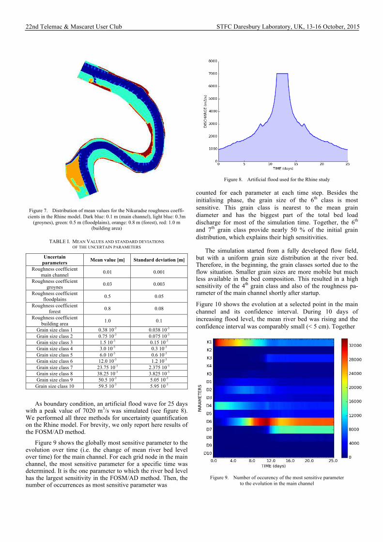
Figure 3 presents the close agreement between the three methods for the standard deviations of the water depth and the scalar velocity (the absolute value of the velocity vector). The uncertainty of water depth is high at the inflow and decreases gradually to zero at the outflow, because the water depth is given there as boundary condition. The uncertainty of scalar velocity concentrated mostly in the second groyne field. The standard deviation in the main channel is small (< 1mm/s) and nearly constant along the flow length. Due to the absence of groynes in the inflow and outflow cross sections, the flow direction is not parallel to the bend anymore. This leads to higher uncertainties at the outflow.

To quantify agreement between the three methods, we in-troduced a similarity index based on a threshold of accuracy (ta). The similarity index is defined as a triangle fuzzy number with base (-ta, ta). It is zero if the difference between two val-ues is larger (smaller) than the upper (lower) threshold ta (-ta) and increases to one if the two values are exactly equal. The threshold value depends on the accuracy of available data and the scale of the problem. For this case, a threshold of 1mm for the water depth seems to be feasible. Figure 4 proves the good agreement between the methods, as the similarity index of FOSM/ND to MC and FOSM/AD to MC is mostly around one except for the second groyne field. This disagreement between the linear FOSM method and MC indicates highly non-linear effects in the affected region.

To verify the linearity assumption in the FOSM approach, we conducted a test for normality: Only if the parameter-to-prediction relations in a model are linear, the assumed Gaussi-an distribution for input parameters results in Gaussian distri-butions for all model predictions. The result of the normality test is the probability for each grid cell that the respective 1000 Monte-Carlo values could in fact originate from a Gaussian distribution (see figure 5). For the water depth, all probabilities to be Gaussian are near one, which validates the applicability of FOSM methods. For the scalar velocity, Gaussianity (and hence linearity) is only present in the main channel. Small probability values in the groyne fields show the non-linearity in these regions.

Figure 3. Comparison of standard deviation of water depth (left) and scalar velocity (right) in the domain computed by FOSM/ND (top), FOSM/AD

(middle), MC (bottom)

22nd Telemac & Mascaret User Club STFC Daresbury Laboratory, UK, 13-16 October, 2015

Figure 4. Distribution of similarity index for comparison of FOSM/ND to MC (top) and FOSM/AD to MC (bottom)

Although the velocities in the groyne fields have little agreement with a Gaussian distribution, our results indicate that the variance or standard deviation still can be estimated with satisfying results by FOSM methods – at least for the degree of uncertainty in the roughness coefficients considered here.

Figure 5. Map of the probabilities that the Monte-Carlo results indicate a Gaussian probability distribution

b. Numerical experiment in transient flow

For the comparison on time-dependent problems, we im-plemented an artificial flood hydrograph for three hours. The inflow discharge increased over 1.5 hours from 22 l/s to 156 l/s and then decreased back to the initial value.

In order to compare FOSM/ND and FOSM/AD with MC, we averaged the similarity indices of the standard deviation over the whole domain in each time step. Figure 6 presents the resulting averaged similarity indices for water depth and scalar velocity over time. Again, only minor differences between FOSM/ND and FOSM/AD can be seen. All similarity indices lay above 0.88, which we interpret as indication of linear or only weakly non-linear behaviour. As expected, the velocities show smaller similarity (i.e. more pronounced non-linear be-haviour). The most non-linear periods occur when the height of the groynes equals the water level. Due to thresholds for wet-ting and drying procedures, the numeric solution is less smooth for this state. We conclude that FOSM provides satisfying results also for time dependent problems for the uncertainties of water levels and velocities – at least for the degree of uncer-tainty in the roughness coefficients considered here.

B. River Rhine model

The central reach of the Lower Rhine between Neuss and Düsseldorf (Rh-km 739-749) was chosen as in-situ application. In the project “artificial grain-feeding of bed material on the central Lower Rhine”, a two-dimensional numerical sediment transport model for this region was developed by the BAW. The aim of the project was to enhance the efficiency of future hydrological design and to optimise the measures economical-ly. Further model details can be found in [10].This part of the river is characterised by strong meandering, dynamic bed load transport and an intensive bed load management. For this study, the dredging and supplying measures were not taken into account.

Figure 6. The average similarity index (FOSM/ND to MC, FOSM/AD to MC) for the flood period

22nd Telemac & Mascaret User Club STFC Daresbury Laboratory, UK, 13-16 October, 2015

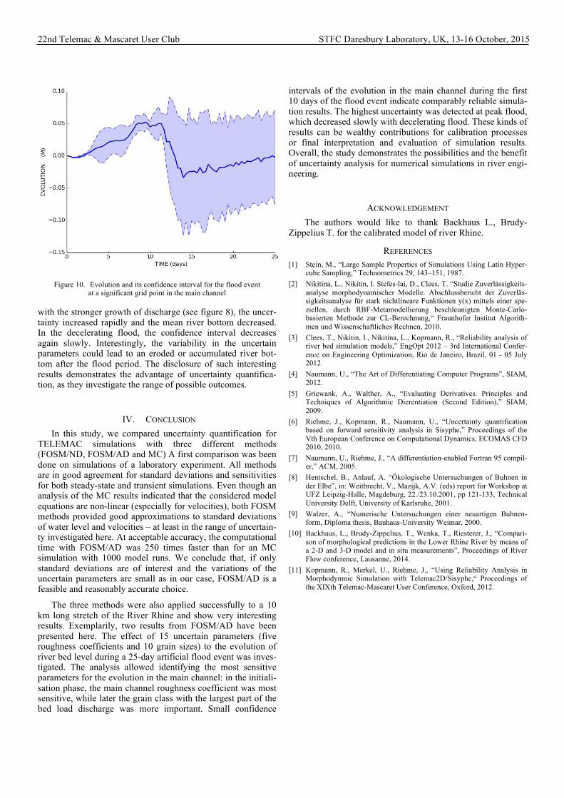
Figure 7. Distribution of mean values for the Nikuradse roughness coeffi-cients in the Rhine model. Dark blue: 0.1 m (main channel), light blue: 0.3m

(groynes), green: 0.5 m (floodplains), orange: 0.8 m (forest), red: 1.0 m (building area)

TABLE I. MEAN VALUES AND STANDARD DEVIATIONS OF THE UNCERTAIN PARAMETERS

Uncertain

parameters Mean value [m] Standard deviation [m]

Roughness coefficient main channel

0.01 0.001

Roughness coefficient groynes

0.03 0.003

Roughness coefficient floodplains

0.5 0.05

Roughness coefficient forest

0.8 0.08

Roughness coefficient building area

1.0 0.1

Grain size class 1 0.38 10-3 0.038 10-3 Grain size class 2 0.75 10-3 0.075 10-3 Grain size class 3 1.5 10-3 0.15 10-3 Grain size class 4 3.0 10-3 0.3 10-3 Grain size class 5 6.0 10-3 0.6 10-3 Grain size class 6 12.0 10-3 1.2 10-3 Grain size class 7 23.75 10-3 2.375 10-3 Grain size class 8 38.25 10-3 3.825 10-3 Grain size class 9 50.5 10-3 5.05 10-3

Grain size class 10 59.5 10-3 5.95 10-3

As boundary condition, an artificial flood wave for 25 days with a peak value of 7020 m3/s was simulated (see figure 8). We performed all three methods for uncertainty quantification on the Rhine model. For brevity, we only report here results of the FOSM/AD method.

Figure 9 shows the globally most sensitive parameter to the evolution over time (i.e. the change of mean river bed level over time) for the main channel. For each grid node in the main channel, the most sensitive parameter for a specific time was determined. It is the one parameter to which the river bed level has the largest sensitivity in the FOSM/AD method. Then, the number of occurrences as most sensitive parameter was

Figure 8. Artificial flood used for the Rhine study

counted for each parameter at each time step. Besides the initialising phase, the grain size of the 6th class is most sensitive. This grain class is nearest to the mean grain diameter and has the biggest part of the total bed load discharge for most of the simulation time. Together, the 6th and 7th grain class provide nearly 50 % of the initial grain distribution, which explains their high sensitivities.

The simulation started from a fully developed flow field, but with a uniform grain size distribution at the river bed. Therefore, in the beginning, the grain classes sorted due to the flow situation. Smaller grain sizes are more mobile but much less available in the bed composition. This resulted in a high sensitivity of the 4th grain class and also of the roughness pa-rameter of the main channel shortly after startup.

Figure 10 shows the evolution at a selected point in the main channel and its confidence interval. During 10 days of increasing flood level, the mean river bed was rising and the confidence interval was comparably small (< 5 cm). Together

Figure 9. Number of occurency of the most sensitive parameter to the evolution in the main channel

22nd Telemac & Mascaret User Club STFC Daresbury Laboratory, UK, 13-16 October, 2015

Figure 10. Evolution and its confidence interval for the flood event at a significant grid point in the main channel

with the stronger growth of discharge (see figure 8), the uncer-tainty increased rapidly and the mean river bottom decreased. In the decelerating flood, the confidence interval decreases again slowly. Interestingly, the variability in the uncertain parameters could lead to an eroded or accumulated river bot-tom after the flood period. The disclosure of such interesting results demonstrates the advantage of uncertainty quantifica-tion, as they investigate the range of possible outcomes.

IV. CONCLUSION

In this study, we compared uncertainty quantification for TELEMAC simulations with three different methods (FOSM/ND, FOSM/AD and MC) A first comparison was been done on simulations of a laboratory experiment. All methods are in good agreement for standard deviations and sensitivities for both steady-state and transient simulations. Even though an analysis of the MC results indicated that the considered model equations are non-linear (especially for velocities), both FOSM methods provided good approximations to standard deviations of water level and velocities – at least in the range of uncertain-ty investigated here. At acceptable accuracy, the computational time with FOSM/AD was 250 times faster than for an MC simulation with 1000 model runs. We conclude that, if only standard deviations are of interest and the variations of the uncertain parameters are small as in our case, FOSM/AD is a feasible and reasonably accurate choice.

The three methods were also applied successfully to a 10 km long stretch of the River Rhine and show very interesting results. Exemplarily, two results from FOSM/AD have been presented here. The effect of 15 uncertain parameters (five roughness coefficients and 10 grain sizes) to the evolution of river bed level during a 25-day artificial flood event was inves-tigated. The analysis allowed identifying the most sensitive parameters for the evolution in the main channel: in the initiali-sation phase, the main channel roughness coefficient was most sensitive, while later the grain class with the largest part of the bed load discharge was more important. Small confidence

intervals of the evolution in the main channel during the first 10 days of the flood event indicate comparably reliable simula-tion results. The highest uncertainty was detected at peak flood, which decreased slowly with decelerating flood. These kinds of results can be wealthy contributions for calibration processes or final interpretation and evaluation of simulation results. Overall, the study demonstrates the possibilities and the benefit of uncertainty analysis for numerical simulations in river engi-neering.

ACKNOWLEDGEMENT

The authors would like to thank Backhaus L., Brudy-Zippelius T. for the calibrated model of river Rhine.

REFERENCES

[1] Stein, M., “Large Sample Properties of Simulations Using Latin Hyper-cube Sampling,” Technometrics 29, 143–151, 1987.

[2] Nikitina, L., Nikitin, I. Stefes-lai, D., Clees, T. “Studie Zuverlässigkeits-analyse morphodynamischer Modelle. Abschlussbericht der Zuverläs-sigkeitsanalyse für stark nichtlineare Funktionen y(x) mittels einer spe-ziellen, durch RBF-Metamodellierung beschleunigten Monte-Carlo-basierten Methode zur CL-Berechnung,“ Fraunhofer Institut Algorith-men und Wissenschaftliches Rechnen, 2010.

[3] Clees, T., Nikitin, I., Nikitina, L., Kopmann, R., “Reliability analysis of river bed simulation models,” EngOpt 2012 – 3rd International Confer-ence on Engineering Optimization, Rio de Janeiro, Brazil, 01 - 05 July 2012

[4] Naumann, U., “The Art of Differentiating Computer Programs”, SIAM, 2012.

[5] Griewank, A., Walther, A., “Evaluating Derivatives. Principles and Techniques of Algorithmic Dierentiation (Second Edition),” SIAM, 2009.

[6] Riehme, J., Kopmann, R., Naumann, U., “Uncertainty quantification based on forward sensitivity analysis in Sisyphe,” Proceedings of the Vth European Conference on Computational Dynamics, ECOMAS CFD 2010, 2010.

[7] Naumann, U., Riehme, J., “A differentiation-enabled Fortran 95 compil-er,” ACM, 2005.

[8] Hentschel, B., Anlauf, A. “Ökologische Untersuchungen of Buhnen in der Elbe”, in: Weitbrecht, V., Mazijk, A.V. (eds) report for Workshop at UFZ Leipzig-Halle, Magdeburg, 22./23.10.2001, pp 121-133, Technical University Delft, University of Karlsruhe, 2001.

[9] Walzer, A., “Numerische Untersuchungen einer neuartigen Buhnen-form, Diploma thesis, Bauhaus-University Weimar, 2000.

[10] Backhaus, L., Brudy-Zippelius, T., Wenka, T., Riesterer, J., “Compari-son of morphological predictions in the Lower Rhine River by means of a 2-D and 3-D model and in situ measurements”, Proceedings of River Flow conference, Lausanne, 2014.

[11] Kopmann, R., Merkel, U., Riehme, J., “Using Reliability Analysis in Morphodynmic Simulation with Telemac2D/Sisyphe,“ Proceedings of the XIXth Telemac-Mascaret User Conference, Oxford, 2012.

IMPLEMENTATION OF A NEW TURBULENCE MODEL IN TELEMAC2D/3D : MODIFIED

SPALART-ALLMARAS :

Adrien Bourgouin Riadh ATA

LNHE-EDF R&D

This model is a RANS turbulence model which solves one transport equation for a viscosity like

variable. As it was designed for aerodynamic flows[1], the set of constants has been adapted for free

surface cases, in order to stabilize it and to get more coherent results. It has been implemented in

Telemac-2D and Telemac-3D and tested with several examples, such as « pildepon ».

Obtained results have been compared to the experimental results of Negretti [2] for the case of a

flow around a cylindrical obstacle (figure 1). The chaarcterization of eddy detachment was achieved

using a non-dimensional number. This non dimensional numer links the effects of lateral boundary

and bottom friction with the geometrical property of the domain/obstacle. Encouraging results are

obtained with this new model. Obtained results are compared to those obtained with K-eps model

and some measurements as well.

Référence :

[1] : P. R. Spalart, S. R. Allmaras :One-Equation Turbulence Model for Aerodynamic Flows.

[2] : M. E. Negretti, G. Vignoli, M. Tubino, M. Brocchini : One Shallow-water Wakes : an

analytical study.