Fundamentals of spatial vision in the barn owl (Tyto alba pratincola): Ocular aberrations, grating acuity, contrast sensitivity, and vernier acuity Von der Fakult¨ at f ¨ ur Mathematik, Informatik und Naturwissenschaften der Rheinisch-Westf¨ alischen Technischen Hochschule Aachen zur Erlangung des akademischen Grades eines Doktors der Naturwissenschaften genehmigte Dissertation vorgelegt von Diplom-Biologe Wolf Maximilian Harmening aus K ¨ oln Berichter : Universit¨ atsprofessor Dr. Hermann Wagner Universit¨ atsprofessor Dr. Frank Schaeffel Tag der m¨ undlichen Pr ¨ ufung: 25. M¨ arz 2008 Diese Dissertation ist auf den Internetseiten der Hochschulbibliothek online verf¨ ugbar.
Transcript
Fundamentals of spatial vision in the barn owl(Tyto alba pratincola):
Ocular aberrations, grating acuity,contrast sensitivity, and vernier acuity
Von der Fakultat fur Mathematik, Informatik und Naturwissenschaftender Rheinisch-Westfalischen Technischen Hochschule Aachen
zur Erlangung des akademischen Gradeseines Doktors der Naturwissenschaften
genehmigte Dissertation
vorgelegt von
Diplom-BiologeWolf Maximilian Harmening
aus Koln
Berichter : Universitatsprofessor Dr. Hermann WagnerUniversitatsprofessor Dr. Frank Schaeffel
Tag der mundlichen Prufung: 25. Marz 2008
Diese Dissertation ist auf den Internetseiten der Hochschulbibliothek online verfugbar.
How does the world look like through the eyes of an animal?
Intriguing as the question may sound at first sight, it might be an impossibletask to give a satisfyingly comprehensive answer. Nevertheless, within the fieldof neuroscience, more effort has gone into studying the visual system than anyother sensory modality, in humans as well as in animals. The key objective ofvisual neuroscience is to explain how the brain transforms retinal images intothe coherent visual world we experience everyday. This might be undertaken atthe very microscopic scale, finding out about how the physical energy of light istransformed into physiological signals, and how those are further processed —or on a more holistic scale, precisely describing how observers react to visualstimulation, ultimately preparing the ground to understand the perceptual high-level process of seeing.
The aim of this thesis was to elaborate some of the most fundamental functionalaspects of spatial vision in an animal that is by nature a truly specialized ani-mal: the barn owl. This was done both at the very first stages of vision, as wellas at later perceptual stages, involving the animals to participate in behavioralexperiments. Specifically, the objectives of the thesis were:
• to study the optical properties of barn owl eyes with the help of state-of-the-art aberrometry techniques,
• to address the neural portion of spatial vision in this bird by psychophys-ical measurements of its contrast sensitivity function and grating acuitythreshold, and finally
• to describe neural enhancements of the owl’s visual experience, allowingit to detect tiny spatial details beyond the limit set by the resolution oftheir eyes, studied in a series of hyperacuity experiments.
1
1 Introduction
1.1 Optical properties of vision
When light enters the eye it is refracted due to its different velocities of propa-gation in the different ocular media, and an inverted image of the visual sceneis formed at the nervous back of the eye, the retina. The accuracy of this pro-cess, and, ultimately, the quality of the retinal image, is dependent on severalphysical constraints.
Foremost, the refractive surfaces of the eye, the cornea and the ocular lens,have the largest impact on image formation. The shape of the cornea and lenswill cause light rays to refract to a distinct degree. In all eyes that have beentested so far, the shape of the refracting surfaces show tiny irregularities, caus-ing the incident light to refract in a slightly irregular manner. As a result ofthese ocular aberrations, the retinal image will be blurred. Furthermore, thelens of most vertebrates has accommodative properties, being able to change itsrefractive power to bring objects of different distances into focus. If the accom-modative capabilities are insufficient to meet the optical requirements given bythe eye’s geometry (i.e. the observer is ametropic), retinal image quality willbe degraded. Other optical side effects, like scatter-light and stray-light, candegrade image quality to unfeasible degrees as well.
Another origin of retinal image degradation is diffraction. Diffraction isthe breaking up of a beam of light when it passes a sharp edge of an opaqueobject. In the vertebrate lens-eye, diffraction is present due to the pupil, a smallopening of variable size that allows control of the total amount of light passedonto the retina. If light originating from a point light source passes the pupil, itis diffracted. The spread light will produce a series of dark and light bands thatinterfere with each other to form the so called Airy-disc, an expanded area ofvariable brightness. This image degradation is also experienced as retinal blur.The amount of blur due to diffraction depends on the size of the pupil, withlarge pupils producing less diffraction (Campbell and Gubisch, 1966).
A state-of-the-art technique that is well suited to measure the influence ofthe afore mentioned physical properties on the image forming process, is wave-front aberrometry. This objective measuring technique, described in detail inchapter 3 (starting on page 27), was applied to assess the optical quality ofthe barn owl eye. The eye’s point-spread function (PSF), its modulation trans-fer function (MTF), and theoretical retinal image quality were calculated fromwavefront maps that were measured in eight barn owl eyes.
2
1.2 Limits of spatial vision
1.2 Limits of spatial vision
After the formation of an image on the retina, may it be perfectly crisp or des-perately blurry, the largest part of the process of vision is yet to take place, andthe question of what the observer actually sees is far from being resolved. Oneof the common approaches to gain insights into the visual world an observerexperiences, is to specify the limits of the observer’s visual capabilities, or,expressed in more psychophysical terms, to measure the observer’s perceptualthreshold for a given visual task. With long standing tradition, a sensible firststep is to measure the observers visual acuity.
Visual acuity
The term visual acuity refers to the ability of an observer to resolve fine spatialdetails in a visual scene. It is bequeathed that, in ancient times, resolving powerof human observers was measured by the ability to separate nearby double starsor clusters, like Mizar and Alcor in the handle of the Big Dipper (Morgan,1991), those being 12 arcmin apart. Given the fixed distance between thoseobjects, the estimate of resolving power was coarse. Nowadays, the observer’sacuity can be estimated precisely using a typical eye chart in an optometrist’soffice (figure 1.1 a). Alternatively, it can be measured by determining the ob-server’s discrimination threshold in a simple visual task similar to those shownin figure 1.1 (b–c).
In all those tasks typical thresholds are in the range of 30–60 arcsec (Camp-bell and Green, 1965b), resembling the average distance between adjacent pho-toreceptors in the most sensitive part of the retina, the fovea (Curcio et al.,1990). As positional information in the photoreceptor-layer is passed to theganglion-cell layer and from there further up the optical nerve to higher brainareas, visual acuity largely depends on the particular way this connection is es-tablished. Positional information is preserved best, it seems, if single ganglioncells receive input from single photoreceptors, and hence their receptive fieldis as small as possible (Merigan and Katz, 1990).
In this thesis, visual acuity of the barn owl was measured with adaptive psy-chophysical techniques. Three barn owls were trained to discriminate gratingsof different orientation. In the course of the experiments, the spatial frequencyof the grating was increased until the owl’s discrimination threshold was de-termined. Grating acuity results from one animal are presented in chapter 4(starting on page 45).
3
1 Introduction
Contrast sensitivity
A next step in characterizing an observer’s visual experience, is to describevisual processing for objects that are larger than the resolution limit. One keyfeature that makes objects distinguishable is the amount of luminance that isreflected relative to the background or relative to other objects. This relativeluminance difference is referred to as luminance-contrast, or simply contrast.
The so-called spatial contrast sensitivity function (CSF) relates the ability ofan observer to visually detect spatial gratings of different spatial frequencies tothe amount of contrast present in the grating. If measured behaviorally, the CSFincorporates visual functions of both physical (i.e. the visual transfer functionof the eye) and, to a greater extent, physiological nature (i.e. visual processingin the nervous system). The CSF may, therefore, be regarded as one of thefundamental functional descriptions of a visual system.
In human observers and virtually any animal that has been tested so far, theCSF renders a band-limited inverted U-shaped function, with a typical high-and low-frequency attenuation. The high frequency roll-off in humans is re-garded as a combined consequence of physical constraints leading to opticaldegradation (such as the diffraction limit and ocular aberrations), and receptorcell spacing on retina level (Campbell and Green, 1965a; Cornsweet, 1970).The low frequency attenuation can be explained solely by neural factors, suchas extent of lateral inhibition (Cornsweet, 1970), antagonistic surround mech-anisms (Westheimer, 1972), or relative insensitivity of low spatial frequencyfilters (Graham, 1972).
Spatial contrast sensitivity was determined in the barn owl in a series of be-havioral experiments, similar to the ones described in the preceding section.The owls had to discriminate the orientation of gratings for eleven differentspatial frequencies. With the appliance of an adaptive staircase procedure,contrast was lowered until discrimination performance reached threshold level.The inverse of threshold was defined as contrast sensitivity and composed theprogression of the contrast sensitivity function. These results are also presentedin chapter 4.
1.3 Hyperacuity phenomena
As demonstrated in the previous section, the ability of humans to resolve finespatial details is limited by the physical nature of light, the optical properties
4
1.3 Hyperacuity phenomena
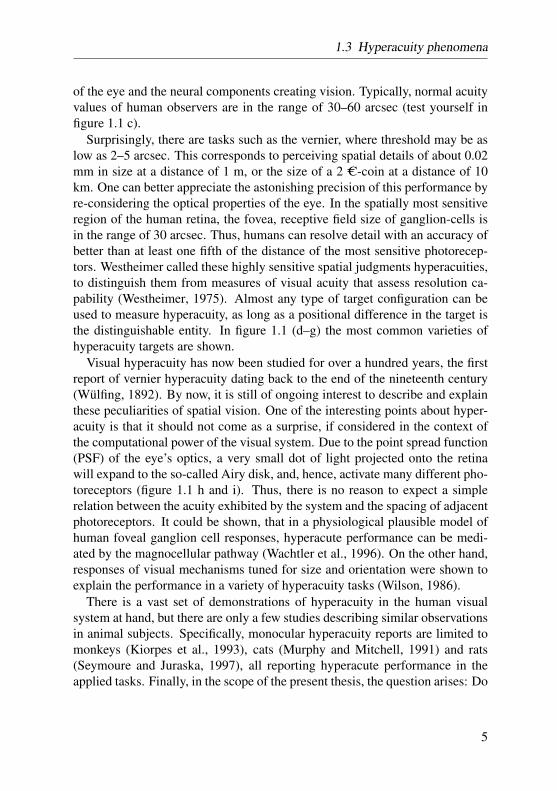
of the eye and the neural components creating vision. Typically, normal acuityvalues of human observers are in the range of 30–60 arcsec (test yourself infigure 1.1 c).
Surprisingly, there are tasks such as the vernier, where threshold may be aslow as 2–5 arcsec. This corresponds to perceiving spatial details of about 0.02mm in size at a distance of 1 m, or the size of a 2 C-coin at a distance of 10km. One can better appreciate the astonishing precision of this performance byre-considering the optical properties of the eye. In the spatially most sensitiveregion of the human retina, the fovea, receptive field size of ganglion-cells isin the range of 30 arcsec. Thus, humans can resolve detail with an accuracy ofbetter than at least one fifth of the distance of the most sensitive photorecep-tors. Westheimer called these highly sensitive spatial judgments hyperacuities,to distinguish them from measures of visual acuity that assess resolution ca-pability (Westheimer, 1975). Almost any type of target configuration can beused to measure hyperacuity, as long as a positional difference in the target isthe distinguishable entity. In figure 1.1 (d–g) the most common varieties ofhyperacuity targets are shown.
Visual hyperacuity has now been studied for over a hundred years, the firstreport of vernier hyperacuity dating back to the end of the nineteenth century(Wulfing, 1892). By now, it is still of ongoing interest to describe and explainthese peculiarities of spatial vision. One of the interesting points about hyper-acuity is that it should not come as a surprise, if considered in the context ofthe computational power of the visual system. Due to the point spread function(PSF) of the eye’s optics, a very small dot of light projected onto the retinawill expand to the so-called Airy disk, and, hence, activate many different pho-toreceptors (figure 1.1 h and i). Thus, there is no reason to expect a simplerelation between the acuity exhibited by the system and the spacing of adjacentphotoreceptors. It could be shown, that in a physiological plausible model ofhuman foveal ganglion cell responses, hyperacute performance can be medi-ated by the magnocellular pathway (Wachtler et al., 1996). On the other hand,responses of visual mechanisms tuned for size and orientation were shown toexplain the performance in a variety of hyperacuity tasks (Wilson, 1986).
There is a vast set of demonstrations of hyperacuity in the human visualsystem at hand, but there are only a few studies describing similar observationsin animal subjects. Specifically, monocular hyperacuity reports are limited tomonkeys (Kiorpes et al., 1993), cats (Murphy and Mitchell, 1991) and rats(Seymoure and Juraska, 1997), all reporting hyperacute performance in theapplied tasks. Finally, in the scope of the present thesis, the question arises: Do
5
1 Introduction
EF P
T O Z
L P E D
P E C F D
E D F C Z P
F E L O P Z D
B A R N O W L
a
d
h i
e f g
b c
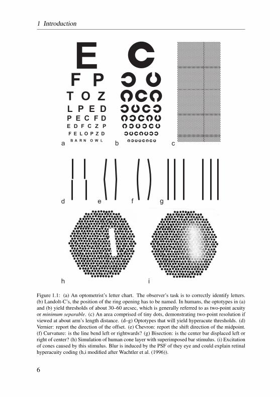
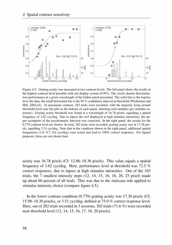
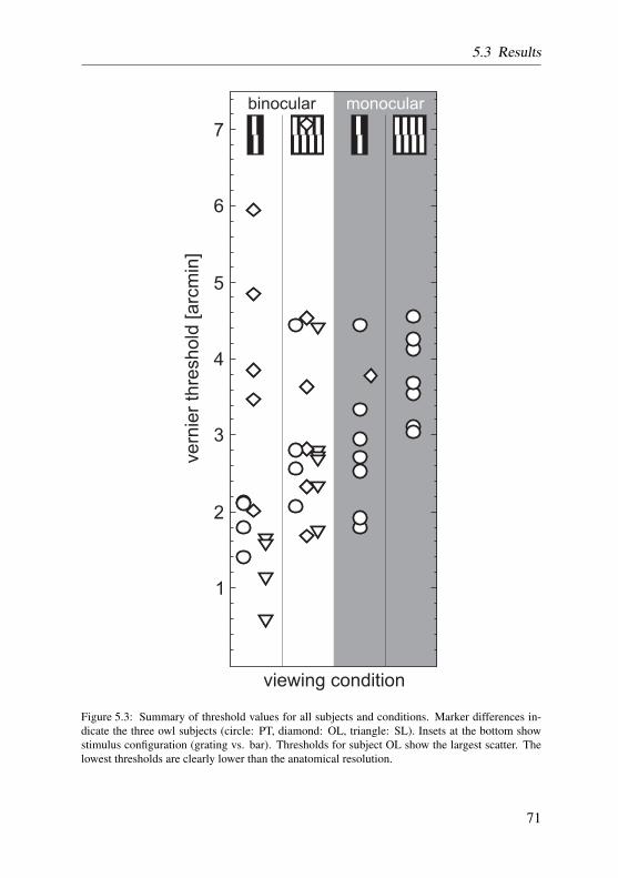
Figure 1.1: (a) An optometrist’s letter chart. The observer’s task is to correctly identify letters.(b) Landolt-C’s, the position of the ring opening has to be named. In humans, the optotypes in (a)and (b) yield thresholds of about 30–60 arcsec, which is generally referred to as two-point acuityor minimum separable. (c) An area comprised of tiny dots, demonstrating two-point resolution ifviewed at about arm’s length distance. (d–g) Optotypes that will yield hyperacute thresholds. (d)Vernier: report the direction of the offset. (e) Chevron: report the shift direction of the midpoint.(f) Curvature: is the line bend left or rightwards? (g) Bisection: is the center bar displaced left orright of center? (h) Simulation of human cone layer with superimposed bar stimulus. (i) Excitationof cones caused by this stimulus. Blur is induced by the PSF of they eye and could explain retinalhyperacuity coding (h,i modified after Wachtler et al. (1996)).
6
1.4 Barn owl vision
birds have hyperacute vision? In chapter 5 of this thesis (starting on page 65),this issue is addressed in a series of psychophysical experiments, measuringthe discrimination threshold for typical vernier stimuli in the barn owl visualsystem. Additionally, to account for possible task difficulty differences, twodifferent vernier stimuli were used as targets, each presented under monocularand binocular viewing conditions.
1.4 Barn owl vision
Early vision: the barn owl eye and retina
In general, birds are highly visual animals. The avian globe, in relation to thesize of the skull, is very large, advantageous to allow a larger image to be pro-jected onto the retina, and thus to contribute vastly to visual acuity (Gunturkun,2000). In birds, approximately 50% or more of the cranial volume of the skullis occupied by the eye, whereas in humans, the eye occupies less than 5% ofthe skulls volume (Waldvogel, 1990).
The eyes of the barn owl, with an axial length of about 17.5 mm, are clearlysmaller than those of humans (24.5 mm) (Hughes, 1977; Schaeffel and Wagner,1996), but according to a study by Howland, barn owl eyes are almost twiceas long as allometry based on body weight would suggest (Howland et al.,2004). Typical for all avian eyes, the nearly hemispheric posterior region of theglobe is disproportionately larger than the anterior segment (Kern, 1991, 1997).The anterior and posterior segments of the globe are united by an intermediateregion based on the scleral ossicles (Murphy and Dubelzieg, 1993). The overallshape of the barn owl eye is tubular (figure 1.2 c) – typical for owls –, in whicha concave intermediate segment is elongated anteroposteriorly, forming a tubebefore joining the posterior segment at a sharp angle (King and McLelland,1984; Waldvogel, 1990; Kern, 1991, 1997; Gunturkun, 2000). This special eyedesign is believed to improve visual acuity at low light levels due to the largerretinal image with a constrained focal length (Martin, 1982). The ratio betweenfocal length and maximal entrance pupil diameter, the f-number, is comparablylow in the barn owl (1.3, versus 2.1 in humans). This ultimately results in abrighter retinal image, and might be another example for an adaptation to anocturnal lifestyle (Schaeffel and Wagner, 1996).
As a result of the largeness of the globe and its fit within the orbit, anytorsional movement of the globe is strongly limited, although all six extraocular
7
1 Introduction
eye muscles are present (Williams, 1994). In the barn owl, specifically, therewere only minor eye movements reported, with a maximum amplitude of about2° (Steinbach and Money, 1973; Dulac and Knudsen, 1990). However, due to along and flexible neck, barn owls can turn their head quickly to extreme angles,probably to compensate the limitations set by their eyes’ immobility (Knudsenand Konishi, 1979; Knudsen and Knudsen, 1985; Dulac and Knudsen, 1990;Masino and Knudsen, 1993).
As part of the typical lens-eye of vertebrates, barn owl eyes have a transpar-ent, avascular lens, that, together with the cornea, serves to refract incominglight, and to focus it on the retina to create an acute image. The lens can ac-commodate, but, in contrast to mammals, the avian lens has an annular padaround its central core, that might serve as a hydrostatic mechanism for trans-mitting pressure from the ciliary muscle to the central core to facilitate accom-modation (Evans and Martin, 1993). A direct relationship exists between thesize of the annular pad and the degree of accommodative ability (Samuelson,1991). Compared to other owls, the accommodative abilities in barn owls arelarge, amounting to about 6–12 D (Howland et al., 1991; Schaeffel and Wag-ner, 1992). Barn owls also use accommodation as a distance cue for shortdistances (Wagner and Schaeffel, 1991). They are not able to accommodateindependently in both eyes (coupled accommodation) (Schaeffel and Wagner,1992), which might indicate that binocular vision is of elevated importance forthese animals (see also next section on page 9).
The retina of birds is comprised of the typical cell-layers found in othervertebrates. However, there are differences regarding vascularization, mor-phology, and areas of visual acuity that are worth mentioning. First, the vas-cularization of the retina of birds is reduced, and it receives nourishment bythe pecten oculi. The pecten extends from the optic nerve into the vitreouschamber (figure 1.2 d), and by saccadic oscillations of the pecten during eyeand head movements, nourishment is performed via diffusion through the vit-reous body (Pettigrew et al., 1990). The pecten also provides an oxygen gra-dient to the retina (Wingstrand and Munk, 1965), subserves acid-base balance(Brach, 1977), and maintains a constant intraocular temperature (Murphy andDubelzieg, 1993).
Second, the bird retinae contain, as in humans, cones and rods, the formerfunctioning in daylight vision and sharp visual acuity, the latter being devotedto low-light vision and the detection of shapes and motion. While the reti-nae of diurnal birds are dominated by a special double-cone cell type (Meyer,1977a), nocturnal owls, as the barn owl, have rod-dominated retinae, with a
8
1.4 Barn owl vision
mean rod:cone ratio of about 30:3 (Oehme, 1961; Braekevelt, 1993; Braekeveltet al., 1996).
Third, and more important for visual acuity, many birds have specializedregions within the retina capable of producing visual acuity greater than out-side those regions (termed visual streak or area centralis). This is achievedby a larger density of photoreceptors and ganglion cells within these regions.In primate mammals and some birds, these areas display a typical physicaldepression, named fovea. Most raptorial birds are bifoveate, having a fovea lo-cated in the temporal retina in addition to the more common centrally locatedfovea (Meyer, 1977b; Inzunza et al., 1991). Owls have only temporal foveae,and, uniquely to them, those foveae contain primarily rods (Fite, 1973; Fite andRosenfield-Wessels, 1975).
In the barn owl retina, only a scarcely distinct temporal fovea is present(figure 1.2 e after Oehme (1961)). The position of the barn owl fovea coin-cides with a retinal area of elevated ganglion cell density (figure 1.2 d afterWathey and Pettigrew (1989)), and determines the visual axes of both eyes tobe almost parallel (figure 1.2 b). Also, a visual streak with higher ganglioncell density, proceeding from the temporal area centralis to nasal regions couldbe identified (Wathey and Pettigrew, 1989). Assuming that ganglion cells inarea centralis are involved in spatial acuity tasks, it is possible to calculate atheoretical value for visual acuity. It turned out that, with about 8 cyc/deg,theoretical grating acuity is comparably poor in the barn owl. Confirming thistheorized value, a pattern electro-retinogram (PERG) study estimated gratingacuity to be 6.9 cyc/deg (Ghim and Hodos, 2006). Among other raptors andbirds, these results put the barn owl, and owls in general, at the very low endof the acuity spectrum (6–7.5 cyc/deg in the Great horned owl (Fite, 1973), 8cyc/deg in the tawny owl (Martin, 1984), and 6 cyc/deg in the little owl (Porci-atti et al., 1989)). As an outstanding example for high resolution capabilities,acuity values of around 140 cyc/deg have been reported for the wedge-tailedeagle (Aquila audax) (Reymond, 1985).
Later stages: neural components of vision
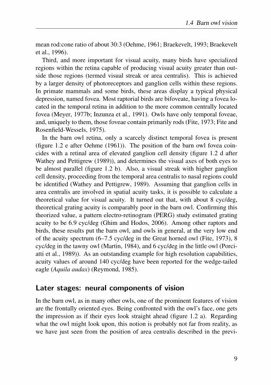
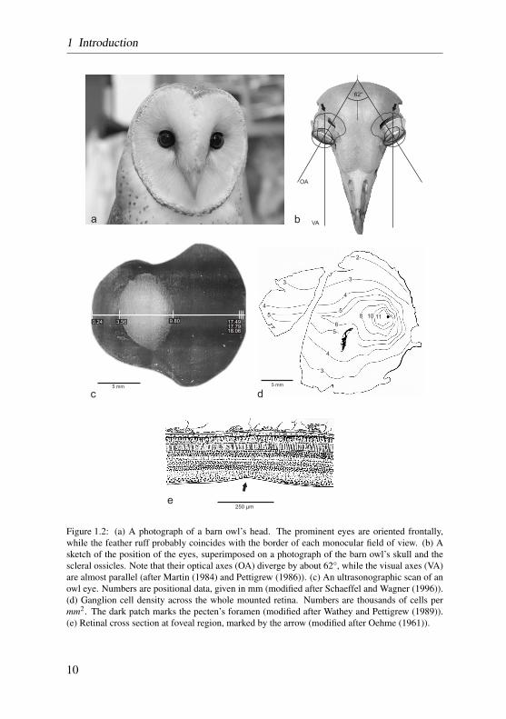
In the barn owl, as in many other owls, one of the prominent features of visionare the frontally oriented eyes. Being confronted with the owl’s face, one getsthe impression as if their eyes look straight ahead (figure 1.2 a). Regardingwhat the owl might look upon, this notion is probably not far from reality, aswe have just seen from the position of area centralis described in the previ-
9
1 Introduction
5 mm
2
6
3
33
8
4
4
4
105
5
511
250 µm
5 mm
a
c
b
d
e
62°
VA
OA
0.24 3.56 9.80 17.4917.7918.06
Figure 1.2: (a) A photograph of a barn owl’s head. The prominent eyes are oriented frontally,while the feather ruff probably coincides with the border of each monocular field of view. (b) Asketch of the position of the eyes, superimposed on a photograph of the barn owl’s skull and thescleral ossicles. Note that their optical axes (OA) diverge by about 62°, while the visual axes (VA)are almost parallel (after Martin (1984) and Pettigrew (1986)). (c) An ultrasonographic scan of anowl eye. Numbers are positional data, given in mm (modified after Schaeffel and Wagner (1996)).(d) Ganglion cell density across the whole mounted retina. Numbers are thousands of cells permm2. The dark patch marks the pecten’s foramen (modified after Wathey and Pettigrew (1989)).(e) Retinal cross section at foveal region, marked by the arrow (modified after Oehme (1961)).
10
1.4 Barn owl vision
ous section. Still, the optical axes in barn owl eyes diverge by approximately62° (Martin, 1984). The geometrical setup of the eyes in the owl skull canbe reviewed in figure 1.2 b. In another nocturnal owl, the tawny owl (Strixaluco), the optical axes diverge to a similar degree, and it has been shown thatthe monocular field of view of the two eyes overlap to form an unusual largebinocular field of view (Martin, 1984).
Though the actual field of view of the barn owl was never measured directly,several other findings revealed that the barn owl indeed has binocular vision.Being stated alone, this fact has no implications further than that objects inthe binocular field of view can be viewed with both eyes at the same time.It was a matter of investigation to find out if the owl uses this geometricalsetting to draw further information out of a visual scene: information that canbe used to extract spatial relations, such as depth and distance. This visualcapability is called stereopsis. To the largest extent, stereopsis relies on theneural comparison of the images falling on the retinae in both eyes. Due tothe different vantage points of the eyes, retinal images differ slightly. Thesedifferences are called disparities, and form the physical foundation from whicha calculation of spatial depth relation is made possible.
It has been shown that the visual Wulst, a part of the avian forebrain which islargely dedicated to visual information processing, show analogies to the pri-mary visual cortex (V1) of mammals as described by Hubel and Wiesel (1962).It turned out that, in the barn owl, the visual Wulst is enlarged and displays se-lectivity for orientation and motion direction (Pettigrew and Konishi, 1976; Liuand Pettigrew, 2003). More interestingly, the visual Wulst exhibits a high de-gree of binocular interaction and selectivity for binocular disparity (Pettigrew,1979; Wagner and Frost, 1993; Nieder and Wagner, 2000). In addition, ina series of seminal psychophysical experiments, it was demonstrated that barnowls indeed use stereopsis as a depth cue. Moreover, the barn owls tested coulddiscriminate random dot stereograms with hyperacute performance (van derWilligen et al., 1998, 2002), a feat that is also present in human and primateobservers (Hadani et al., 1980).
A recent study involving a miniature camera placed on the owl’s foreheadshed light on the attentional mechanisms of vision in this bird. The resultsrevealed that during an active search task, owls repeatedly and consistentlydirect their gaze in a way that brings objects of interest to a specific retinallocation. Additionally, it was suggested a top-down modulation of gaze controlwhen owls view natural targets. (Ohayon et al., 2008). The barn owl’s abilityto visually extract higher level features was further demonstrated in another
11
1 Introduction
behavioral study. Here, it was shown that these animals, as humans, are proneto perceive illusionary contours (Nieder and Wagner, 1999).
1.5 Organization of the thesis
In this first chapter of the thesis, a short introduction to the first stages ofspatial vision was presented. Additionally, the topic of hyperacuity phenom-ena was briefly introduced. To a larger extent, the visual system of the barnowl was reviewed. The second chapter covers the methodological approachI chose to elaborate these fields in the barn owl visual system. General psy-chophysical procedures as well as a description of the technical equipmentused throughout all experiments are given. The main part of the thesis is laiddown in chapters three to five. Here, the results of three different studies arepresented. Specifically, these were, (a) objective measurements of the opticalproperties of barn owl eyes by wavefront aberrometry (Chapter 3), (b) psy-chophysical measurements of the spatial contrast sensitivity function and grat-ing acuity with an orientation discrimination task (Chapter 4), and (c) the de-scription of a hyperacute phenomenon in the barn owl visual system, measuredbehaviorally in monocular and binocular vernier acuity experiments (Chapter5). The sixth chapter of the thesis concludes with a general discussion of thepresented results. It reviews the main findings and their implications, and re-lates to observations made in other animals. Here, the final conclusions aredrawn, addressing the question how the world might look through the eyes ofa barn owl. The last chapter provides a one-page summary of the thesis.
12
1.5 Organization of the thesis
13
1 Introduction
14
2 Materials and Methods
2.1 Animal subjects
In total, 6 adult American barn owls (Tyto alba pratincola) were used as exper-imental animals. Eight eyes of four animals were studied in the wavefront aber-ration experiments, three animals were tested in the vernier acuity experimentsand one animals’ contrast sensitivity and grating acuity was measured. Takenfrom the institute’s breeding stock, all owls were hand-raised and tame. Theycould be easily carried between their aviaries and the experimental room whiletied to a wooden perch. No attempt was made to reverse the owls’ nocturnalcycle. Experiments took place on 5–6 days a week. The owls’ diet consisted ofdead 1-day old domestic chicks and mice. To avoid deficiency symptoms, theowls received an additional vitamin supplement once in two weeks. To ensuremotivation in behavioral tests, the owls’ weight was maintained at about 90 %of their free feeding weight. They were rewarded with small pieces of chickmuscle-tissue, approximately 2 grams in weight. Water was always given adlibitum. All of the subjects carried an aluminium head-post, which was im-planted onto the forehead of their scull under anaesthesia earlier during life.For a detailed description of the surgical procedure and the used drugs refer toNieder and Wagner (1999). In the vernier acuity experiments, the head-postwas used to fix a small custom build spectacle frame to the owls head.
Care and treatment of the subjects was carried out in accordance with theguidelines for animal experimentation as approved by the ”Landesprasidiumfur Natur, Umwelt und Verbraucherschutz Nordrhein Westfalen”, Reckling-hausen, Germany, and complied with the ”NIH Guide for the use and care oflaboratory animals”.
15
2 Materials and Methods
2.2 Procedures in wavefront aberrationexperiments
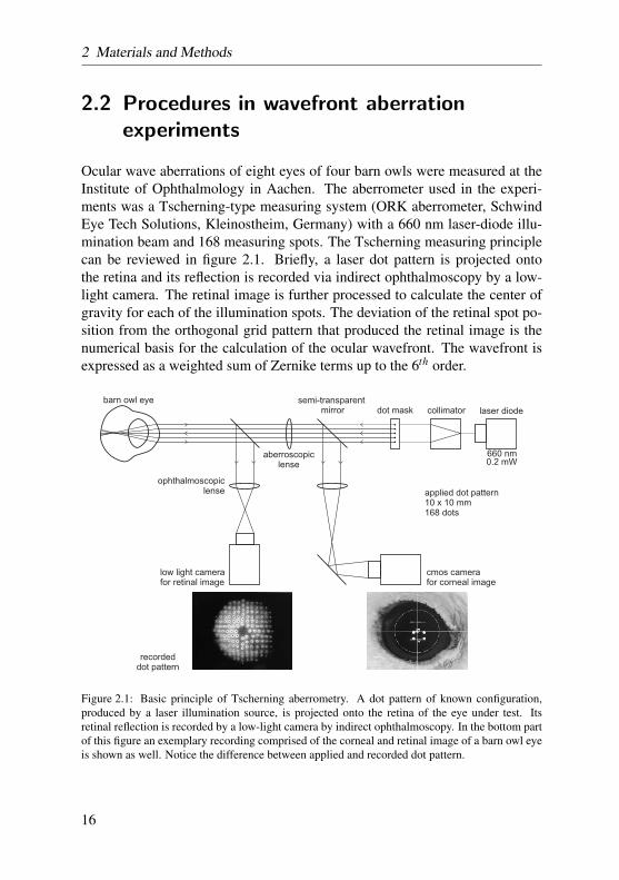
Ocular wave aberrations of eight eyes of four barn owls were measured at theInstitute of Ophthalmology in Aachen. The aberrometer used in the experi-ments was a Tscherning-type measuring system (ORK aberrometer, SchwindEye Tech Solutions, Kleinostheim, Germany) with a 660 nm laser-diode illu-mination beam and 168 measuring spots. The Tscherning measuring principlecan be reviewed in figure 2.1. Briefly, a laser dot pattern is projected ontothe retina and its reflection is recorded via indirect ophthalmoscopy by a low-light camera. The retinal image is further processed to calculate the center ofgravity for each of the illumination spots. The deviation of the retinal spot po-sition from the orthogonal grid pattern that produced the retinal image is thenumerical basis for the calculation of the ocular wavefront. The wavefront isexpressed as a weighted sum of Zernike terms up to the 6th order.
collimatordot mask
applied dot pattern10 x 10 mm168 dots
recordeddot pattern
semi-transparentmirror
ophthalmoscopiclense
aberroscopiclense
cmos camerafor corneal image
low light camerafor retinal image
laser diode
0.2 mW
barn owl eye
660 nm
Figure 2.1: Basic principle of Tscherning aberrometry. A dot pattern of known configuration,produced by a laser illumination source, is projected onto the retina of the eye under test. Itsretinal reflection is recorded by a low-light camera by indirect ophthalmoscopy. In the bottom partof this figure an exemplary recording comprised of the corneal and retinal image of a barn owl eyeis shown as well. Notice the difference between applied and recorded dot pattern.
16
2.2 Procedures in wavefront aberration experiments
a b
c
d
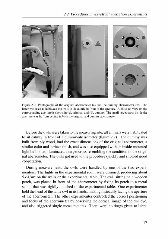
Figure 2.2: Photographs of the original aberrometer (a) and the dummy aberrometer (b). Thelatter was used to habituate the owls to sit calmly in front of the aperture. A close-up view on thecorresponding aperture is shown in (c), original, and (d), dummy. The small target cross inside theaperture was lit from behind in both the original and dummy aberrometer.
Before the owls were taken to the measuring site, all animals were habituatedto sit calmly in front of a dummy-aberrometer (figure 2.2). The dummy wasbuilt from ply wood, had the exact dimensions of the original aberrometer, asimilar color and surface finish, and was also equipped with an inside-mountedlight bulb, that illuminated a target cross resembling the condition in the origi-nal aberrometer. The owls got used to the procedure quickly and showed goodcooperation.
During measurements the owls were handled by one of the two experi-menters. The lights in the experimental room were dimmed, producing about5 cd/m2 on the walls or the experimental table. The owl, sitting on a woodenperch, was placed in front of the aberrometer by fixing its perch to a metalstand, that was rigidly attached to the experimental table. One experimenterheld the head of the tame owl in its hands, making it steadily facing the apertureof the aberrometer. The other experimenter controlled the correct positioningand focus of the aberrometer by observing the corneal image of the owl eye,and also triggered single measurements. There were no drugs given to lubri-
17
2 Materials and Methods
cate the eye, block accommodation or influence pupil size. The owls blinkednormally during the experiments. Each owl was tested in one experimentalsession which took about 2 hours. Each session comprised several individualmeasurements (6–20) for both eyes.
2.3 Procedures in behavioral experiments
2.3.1 Experimental setup
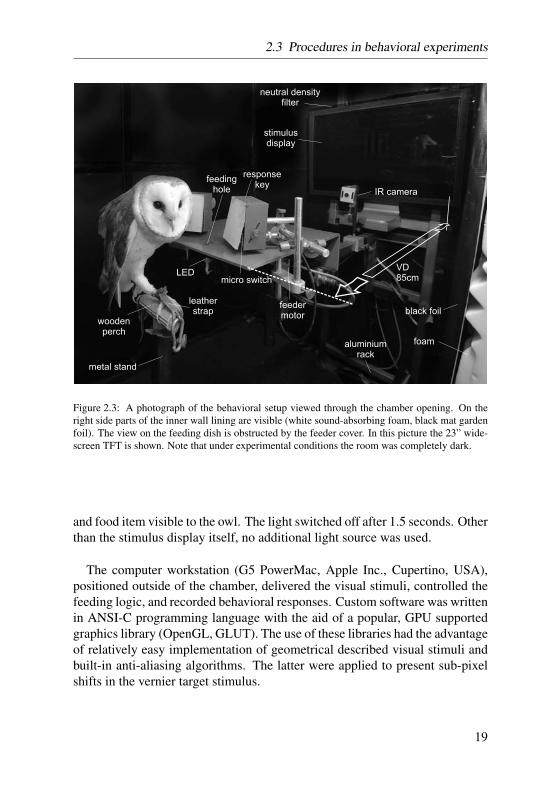
All behavioral experiments were performed in a custom build sound and lightattenuated chamber (outer dimensions: 1.5 x 2 x 1.5 m). The inside walls ofthe chamber were covered with sound-absorbing foam and a black mat gardenfoil to minimize unwanted reflections originating from the stimulus display.A small air fan, invisibly mounted into the ceiling wall, drew fresh air into thechamber, and, additionally, produced a continuous low background noise level.A rigid metal stand placed in easy reach of the chamber opening was used tofix the owl’s sitting perch in front of the response and feeding apparatus. Theautomated feeder with the response keys, the stimulus display and an infraredobservation camera were mounted onto an adjustable aluminium rack that wasrigidly attached to the inner walls of the chamber. An additional infrared cam-era was placed along side the stand of the owl perch. A detailed photograph ofthe chamber interior is shown in figure 2.3.
The response apparatus consisted of two large custom build response keys.Their front plate could be depressed by a light touch of the owls beak. A micro-switch similar as is used in electronic computer mice, produced an audibleclick when the key was pushed correctly. The micro-switches in each of thetwo keys were connected to an USB input interface of the workstation viawiring to the circuit controlling the two main buttons of a standard computermouse. In this way, automatic response recording was possible with easy-to-implement devices and algorithms. The carousel feeder, covered with a topplate leaving reach to the reward food items through a small opening (feedinghole), was driven by a step motor that advanced a rotating acrylic feeding dish(36 single feeding cups per dish). The step motor was controlled via TTL-pulses produced by an USB input/output device (BMC Messsysteme GmbH,Maisach, Germany). This device also automatically triggered a white-lightLED that was mounted below the feeding hole. The LED was switched onwhenever the feeding dish rotated in feeding position, making the feeding cup
18
2.3 Procedures in behavioral experiments
responsekey
micro switch
metal stand
aluminiumrack
foam
black foil
feedinghole
LED
neutral densityfilter
stimulusdisplay
woodenperch
leatherstrap
feedermotor
IR camera
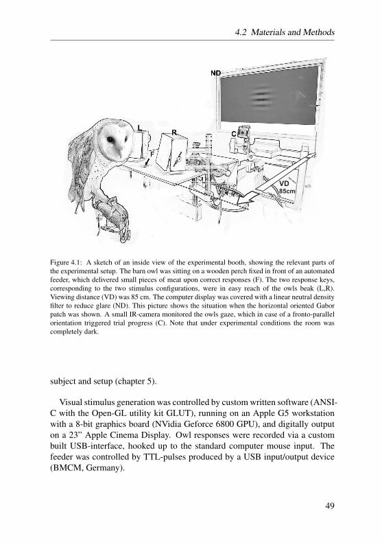
VD85cm
Figure 2.3: A photograph of the behavioral setup viewed through the chamber opening. On theright side parts of the inner wall lining are visible (white sound-absorbing foam, black mat gardenfoil). The view on the feeding dish is obstructed by the feeder cover. In this picture the 23” wide-screen TFT is shown. Note that under experimental conditions the room was completely dark.
and food item visible to the owl. The light switched off after 1.5 seconds. Otherthan the stimulus display itself, no additional light source was used.
The computer workstation (G5 PowerMac, Apple Inc., Cupertino, USA),positioned outside of the chamber, delivered the visual stimuli, controlled thefeeding logic, and recorded behavioral responses. Custom software was writtenin ANSI-C programming language with the aid of a popular, GPU supportedgraphics library (OpenGL, GLUT). The use of these libraries had the advantageof relatively easy implementation of geometrical described visual stimuli andbuilt-in anti-aliasing algorithms. The latter were applied to present sub-pixelshifts in the vernier target stimulus.
19
2 Materials and Methods
2.3.2 Visual stimulation and viewing conditions
All visual stimuli were presented via a computer display. The stimulus displaywas either a 17”-TFT panel (Hansol LCD, Seoul, South Korea) or a wide-screen 23”-TFT panel (Apple Inc.). Both displays were operated at their nativeresolution (1280 x 1024 pixels and 1920 x 1680 pixels, respectively), digitallycontrolled by an 8-bit graphics board (Nvidia GeForce 6800 GPU, Santa Clara,USA). Because the chamber was completely dark, at stimulus onset in CSFexperiments, substantial light intensity changes could occur. To keep glare andunwanted adaptation effects in those cases as low as possible, an additionallarge sheet of neutral density filter was placed in front of the stimulus display(LEE Filters, Andover, UK). The filter lowered overall luminance by 0.92 logunits, with a linear relationship between absolute luminance and luminancereduction.
Stimulus presentation was monitored constantly during experimenting via anadditional computer display that was connected to the second, cloned output ofthe graphics board. This display panel was placed at the experimenter’s tableoutside of the chamber. Here, barn owl’s gaze and general behavior could bemonitored by observation of two small CRTs connected to the infrared cam-eras inside the chamber. Viewing distance was held constant at 85 cm in allbehavioral experiments, but was not measured during experiments. A carefulobservation of the owls’ behavior revealed that, while watching the display, theowls remained in a freezed posture. During fixation, the owls repeatedly heldtheir head directly above the feeding hole, midway between the two responsekeys. In this way, viewing distance could be estimated accurately. At viewingdistance, one pixel subtended 1.052 and 1.044 arcmin, respectively, dependingon the stimulus display (see above).
In the contrast sensitivity measurements, accurate contrast defined stimulihad to be applied. Stimulus contrast was carefully determined by measuringthe luminance of the brightest and darkest parts of the stimulus at the centerof the display at viewing distance. Some calibration procedures were writtento measure luminance quickly for each gray value used in the CSF experi-ments. All luminance measurements were conducted with the Minolta LS-100 luminance-meter (Konica Minolta Medical and Graphic Imaging EuropeGmbH, Munchen, Germany). To produce a linear relationship between grayvalues set in the display system and actually measured luminance values, γ-correction was applied.
In order to deliver monocular stimuli in the vernier acuity experiments, a
20
2.3 Procedures in behavioral experiments
set screw
PVC frame
aluminium
screw socketmetal wire
a b
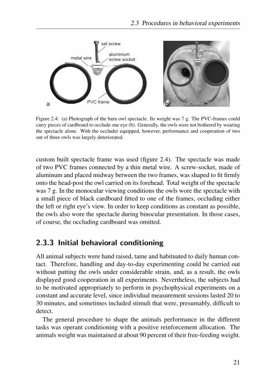
Figure 2.4: (a) Photograph of the barn owl spectacle. Its weight was 7 g. The PVC-frames couldcarry pieces of cardboard to occlude one eye (b). Generally, the owls were not bothered by wearingthe spectacle alone. With the occluder equipped, however, performance and cooperation of twoout of three owls was largely deteriorated.
custom built spectacle frame was used (figure 2.4). The spectacle was madeof two PVC frames connected by a thin metal wire. A screw-socket, made ofaluminum and placed midway between the two frames, was shaped to fit firmlyonto the head-post the owl carried on its forehead. Total weight of the spectaclewas 7 g. In the monocular viewing conditions the owls wore the spectacle witha small piece of black cardboard fitted to one of the frames, occluding eitherthe left or right eye’s view. In order to keep conditions as constant as possible,the owls also wore the spectacle during binocular presentation. In those cases,of course, the occluding cardboard was omitted.
2.3.3 Initial behavioral conditioning
All animal subjects were hand raised, tame and habituated to daily human con-tact. Therefore, handling and day-to-day experimenting could be carried outwithout putting the owls under considerable strain, and, as a result, the owlsdisplayed good cooperation in all experiments. Nevertheless, the subjects hadto be motivated appropriately to perform in psychophysical experiments on aconstant and accurate level, since individual measurement sessions lasted 20 to30 minutes, and sometimes included stimuli that were, presumably, difficult todetect.
The general procedure to shape the animals performance in the differenttasks was operant conditioning with a positive reinforcement allocation. Theanimals weight was maintained at about 90 percent of their free-feeding weight.
21
2 Materials and Methods
Reinforcement was given by small pieces of chick muscle tissue, delivered by acarousel feeder with 36 feeding cups per dish. Usually, two dishes could be fedper day. In this way, owls could be reinforced for the desired behavior aboutseventy times per day. Behavioral shaping was accomplished stepwise. First,the animals had to learn to sit calmly inside the experimental chamber and toreceive rewards from the feeder. In a next step, rewards were only given afterone of the two response buttons was depressed by a touch of the owl’s beak ina pecking-like manoeuver. The animals got used to this concept very fast andusually needed less than two weeks to show successful key pecking.
The next stage was the more difficult part of owl training. The owls wereto peck one of the two keys after they fixated the stimulus display for someseconds. To draw the owl’s attention towards the screen and have them orien-tated correctly towards it, a small bright observation stimulus was presented onthe screen. It had a diamond shape, and changed its brightness constantly ina loop, giving it an overall pulsating appearance. After owls performed wellon this task, the last step was carried out, where task complexity processed tothe final level. The owls had to fixate the observation stimulus for a randomamount of seconds (1–5 s), and were presented afterwards a target stimulusupon which the response keys were released to be pushed. The target stimuluswas drawn randomly from a set of two different stimulus configurations whichcorresponded each to one of the two response keys. That is, if the owl wasgiven target stimulus A, a push of the right response key was rewarded, whilea push of the left response key ended the trial without reward, and returnedthe screen in observation mode again. Consequently, a given target stimulus Breversed this relation. It took about six to nine months of intensive training tofinally have three naive animals to perform reliably in this task. On the otherhand, two other owls used in the studies were already used to visual discrim-ination paradigms and did not have to undergo the above-mentioned trainingsteps. These owls could start in transfer training sessions right away.
2.3.4 Transfer experiments
Transfer training sessions were carried out after the owls mastered in the initialbasic discrimination paradigm, as was introduced above. In transfer sessions,the configuration of training stimuli A and B were altered successively untiltheir appearance arrived at the final configuration A’ and B’, that was actuallyused in the experimental sessions. That is, after the transition from the initialeasy-to-discriminate targets A and B to the final version, A’ and B’ had only
22
2.3 Procedures in behavioral experiments
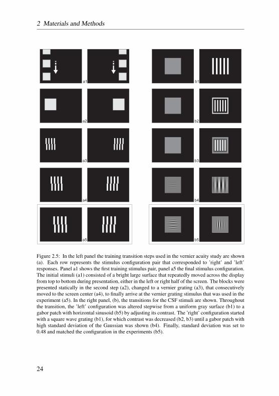
one single distinguishable feature left. In the vernier acuity experiments thisfeature was a horizontal offset in a pair of abutting bars and gratings, and inthe CSF experiments this feature was the orientation of the sinusoid of a Gaborpatch. The transition steps and the final stimulus configuration as were used inthe two different behavioral studies can be reviewed in figure 2.5.
2.3.5 Task design and reward strategy
A prerequisite for perceptual sensitivity measures, such as the discriminationsensitivity for displaced lines in a grating stimulus (vernier acuity), or discrimi-nation sensitivity for the orientation of contrast defined Gabor patches (contrastsensitivity), is the successful perceptual discrimination of the two respectivestimulus configurations. That is, the barn owls had to learn to memorize eachof the two configurations and, on stimulus onset, compare its memory to thepresented stimulus and push the corresponding response key. This approachcan be regarded as an one-interval, two alternative forced choice discrimina-tion task, similar as it is widely used in psychophysical studies. In every ex-perimental condition, the time course of stimulus presentation was self-paced.The birds were, therefore, allowed to examine the stimuli as exact as needed.
As soon as the owls displayed successful discrimination of the training stim-uli, the experimental phase began. We defined the discrimination success asbeing accomplished if the owls performed significantly better than a binomialchance process would govern. As an example, if 100 trials were presented, a99% percent confidence interval would assign that more than 63 trials had tobe correct responses to meet this requirement. Because stimulus alternationfollowed a pseudo-randomized order, allowing no more than three consecu-tive presentation of one of the two alternatives, we raised the significance limitby additional 10 percent. Given the example above, the owls had to be cor-rect in 73 percent of the trials. Generally, when no experiments took place,the owls’ performance was sustained with in-between training sessions. If theowls displayed unreliable performance at high stimulus intensities during anexperimental session, the session was aborted and a normal training sessionfilled the gap.
As in the training sessions, correct responses in experimental sessions wererewarded by food items. Reward contingencies were always 100 percent, giv-ing the animal perfect feedback about the correctness of its choice. This hadthe advantage of less frustration due to unrewarded correct responses, but alsohad the disadvantage such that perceptual learning processes were not neces-
23
2 Materials and Methods
a1 b1
a2 b2
a3 b3
a4 b4
a5 b5
Figure 2.5: In the left panel the training transition steps used in the vernier acuity study are shown(a). Each row represents the stimulus configuration pair that corresponded to ’right’ and ’left’responses. Panel a1 shows the first training stimulus pair, panel a5 the final stimulus configuration.The initial stimuli (a1) consisted of a bright large surface that repeatedly moved across the displayfrom top to bottom during presentation, either in the left or right half of the screen. The blocks werepresented statically in the second step (a2), changed to a vernier grating (a3), that consecutivelymoved to the screen center (a4), to finally arrive at the vernier grating stimulus that was used in theexperiment (a5). In the right panel, (b), the transitions for the CSF stimuli are shown. Throughoutthe transition, the ’left’ configuration was altered stepwise from a uniform gray surface (b1) to agabor patch with horizontal sinusoid (b5) by adjusting its contrast. The ’right’ configuration startedwith a square wave grating (b1), for which contrast was decreased (b2, b3) until a gabor patch withhigh standard deviation of the Gaussian was shown (b4). Finally, standard deviation was set to0.48 and matched the configuration in the experiments (b5).
24
2.3 Procedures in behavioral experiments
sarily to be excluded as an additional factor influencing threshold performance.To minimize this influence, experimental variables, such as stimulus configu-ration in vernier experiments, or spatial frequencies in CSF experiments, werealways applied in roving alternations. If perceptual learning, though, had takenplace, its effect would have influenced the results equally across experimentalconditions, and, as a result, would have ruled out systematic impact.
2.3.6 Psychophysical threshold estimation
In both behavioral studies (vernier acuity and contrast sensitivity experiments)an adaptive staircase was applied to place stimulus intensities adequately for asubsequent estimate of the underlying perceptual threshold. However, thresh-old estimation procedures differed in both studies.
In contrast sensitivity and grating acuity experiments the staircase procedurewas modified according to the two-down, one-up rule. That is, stimulus inten-sities were increased after two consecutive correct responses, and decreased onevery false response. Stimulus intensities, then, converged to levels at whichthe subject responded 70.7% of the time correctly (Treutwein, 1995). Here-after, the ratio of correct responses at each intensity level was calculated andplotted as a function of stimulus intensity. The data was then fitted by a two-parameter logistic function with a bootstrap method described in greater detailby Wichmann and Hill (2001a,b). Threshold performance was set half-waybetween chance level and high-intensity level, accounting for lapses the owldisplayed at high stimulus intensities. The data of two such psychometric func-tions recorded on consecutive days were pooled in order to balance out fluc-tuating performance. For a more detailed description of the procedure reviewsection 4.2.4 on page 51.
In vernier acuity experiments, the discrimination threshold was derived di-rectly from a variable number of reversal points of simple up-down staircasetracks. Two tracks were applied in a randomly interleaved manner and theiroverall threshold was expressed as the arithmetic mean of the thresholds forthe individual tracks. All tracks that were biased according to two differentcriteria were omitted from further analysis. For a more detailed description ofthe procedure review section 5.2.3 on page 68.
25
2 Materials and Methods
26
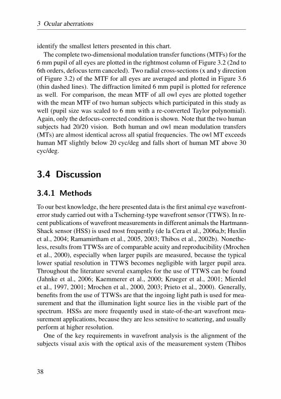
3 Ocular aberrations
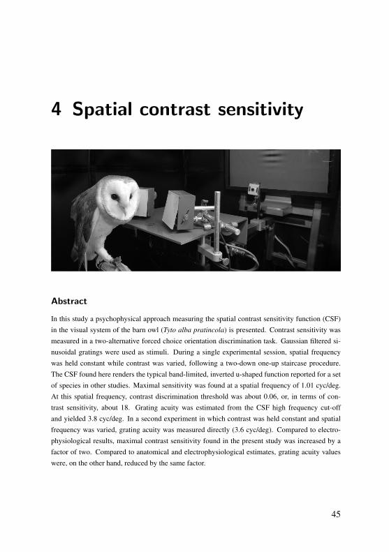
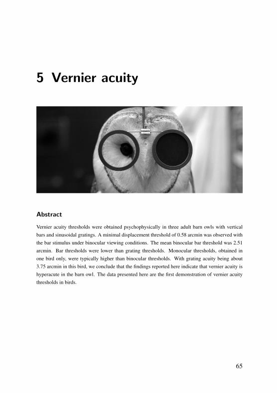
Abstract
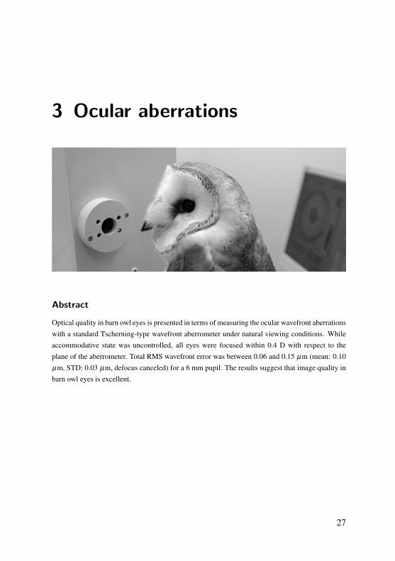
Optical quality in barn owl eyes is presented in terms of measuring the ocular wavefront aberrationswith a standard Tscherning-type wavefront aberrometer under natural viewing conditions. Whileaccommodative state was uncontrolled, all eyes were focused within 0.4 D with respect to theplane of the aberrometer. Total RMS wavefront error was between 0.06 and 0.15 µm (mean: 0.10µm, STD: 0.03 µm, defocus canceled) for a 6 mm pupil. The results suggest that image quality inbarn owl eyes is excellent.
27
3 Ocular aberrations
3.1 Introduction
The barn owl is an excellent candidate for studies of orientation behavior bothin the auditory and visual domain, because it displays several functional, anatom-ical and physiological specializations. The most prominent feature of vision inthese birds are the frontally oriented eyes, which create a large binocular fieldof view, an indicator for increased ethological importance of the use of stereovision (Martin, 1984; Martin and Katzir, 1999; Wagner and Luksch, 1998).Consistently, behavioral studies showed that barn owls possess global stereop-sis and use disparity as a depth cue with hyperacute precision (van der Willigenet al., 1998, 2002, 2003). Electrophysiological studies revealed that the visualWulst of barn owls shows a high degree of binocular interactions and containsdisparity sensitive cells that are tuned to characteristic disparities (Pettigrewand Konishi, 1976; Wagner and Frost, 1993, 1994; Nieder and Wagner, 2000).A more recent study found that barn owls also can discriminate non-alignedfeatures in visual stimuli on a hyperacute level when viewed monocularly, aphenomenon known as vernier acuity in human visual research (refer to chap-ter 5 of this thesis, starting on page 65). This study also pointed to a similarcomputation of vernier targets in humans and owls, because the results in owlsdisplayed a typical crowding/masking effect and a threshold improvement bya similar ratio which is typical for binocular summation in vernier experimentsconducted with human subjects (Banton and Levi, 1991; Malania et al., 2007).
Objective measurements of the metrics of the barn owl eye implicated thatthese eyes are designed to maximize image quality while maintaining an in-creased level of retinal information convergence, advantageous especially un-der low light conditions (Martin, 1982; Schaeffel and Wagner, 1996). With anaxial length of about 17.5 mm, the barn owl eye is relatively large (Schaeffeland Wagner, 1996), being almost twice as long as allometry based on bodyweight would suggest (Howland et al., 2004). Generally, a larger eye resultsin a larger retinal image, and thus, in an improved resolving power. On theother hand, indirect measurements of normal visual acuity (i.e. grating acuityestimation by ganglion cell counts and by pattern electro-retinogram) showedthat visual acuity in these birds is comparably poor (Ghim and Hodos, 2006;Wathey and Pettigrew, 1989). Here, we wanted to find out to what degreevision in the owl is limited by the optical properties of their eyes. For that pur-pose we studied optical quality in means of an objective measurement of theocular wavefront aberrations with a standard Tscherning-type aberrometer in
28
3.2 Materials and Methods
the awake barn owl under natural viewing conditions.Wavefront aberrometry for the assessment of optical quality in human eyes
has been widely used and can also be often found in clinical applications di-rectly linked to eye surgery (Marcos, 2006; Thibos, 2000; Thibos et al., 2002c).Besides human eye studies, the measurement of wave aberrations was also ap-plied in animal eye studies. So far, these include wavefront-error reports in eyesof mice (de la Cera et al., 2006a), cats (Huxlin et al., 2004), chicken (Thiboset al., 2002b), tree shrews (Ramamirtham et al., 2003) and monkeys (Colettaet al., 2003; Ramamirtham et al., 2005, 2006).
3.2 Materials and Methods
3.2.1 Subjects
Experimental animals were four adult American barn owls (Tyto alba prat-incola, three males, one female). Subject ages were between one and threeyears. All owls were taken from the institute’s breeding stock and were hand-raised. They were kept in aviaries throughout their lives. All owls carried a”head-holder”, a small aluminium stick, that was implanted onto the skull oftheir forehead under anaesthesia at an earlier time during life (for details ofthe procedure see Nieder and Wagner (1999)). Animals were kept at aboutninety percent of their free feeding weight, because they participated in otherbehavioral experiments in which food deprivation was essential. A single mea-surement session was conducted with each owl and lasted no longer than threehours. Care and treatment of the owls were carried out in accordance with theguidelines for animal experimentation as approved by the ”Landesprasidium frNatur, Umwelt und Verbraucherschutz Nordrhein Westfalen”, Recklinghausen,Germany, and complied with the ”NIH Guide for the use and care of laboratoryanimals”.
3.2.2 Measurement protocol and aberrometer
All measurements were conducted at the Department of Ophthalmology inAachen. The experimental room was lit dimly by tungsten light, producinga luminance between 2 and 7 cd/m at the walls, the experimental table andthe aberrometer, which matched the luminance of the fixation target inside theaberrometer. Barn owls were sitting on a wooden perch that was attached to
29
3 Ocular aberrations
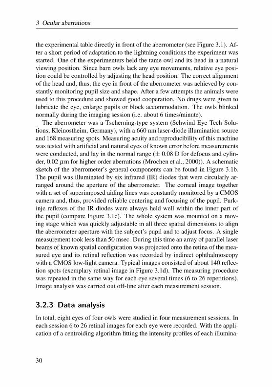
the experimental table directly in front of the aberrometer (see Figure 3.1). Af-ter a short period of adaptation to the lightning conditions the experiment wasstarted. One of the experimenters held the tame owl and its head in a naturalviewing position. Since barn owls lack any eye movements, relative eye posi-tion could be controlled by adjusting the head position. The correct alignmentof the head and, thus, the eye in front of the aberrometer was achieved by con-stantly monitoring pupil size and shape. After a few attempts the animals wereused to this procedure and showed good cooperation. No drugs were given tolubricate the eye, enlarge pupils or block accommodation. The owls blinkednormally during the imaging session (i.e. about 6 times/minute).
The aberrometer was a Tscherning-type system (Schwind Eye Tech Solu-tions, Kleinostheim, Germany), with a 660 nm laser-diode illumination sourceand 168 measuring spots. Measuring acuity and reproducibility of this machinewas tested with artificial and natural eyes of known error before measurementswere conducted, and lay in the normal range (± 0.08 D for defocus and cylin-der, 0.02 µm for higher order aberrations (Mrochen et al., 2000)). A schematicsketch of the aberrometer’s general components can be found in Figure 3.1b.The pupil was illuminated by six infrared (IR) diodes that were circularly ar-ranged around the aperture of the aberrometer. The corneal image togetherwith a set of superimposed aiding lines was constantly monitored by a CMOScamera and, thus, provided reliable centering and focusing of the pupil. Purk-inje reflexes of the IR diodes were always held well within the inner part ofthe pupil (compare Figure 3.1c). The whole system was mounted on a mov-ing stage which was quickly adjustable in all three spatial dimensions to alignthe aberrometer aperture with the subject’s pupil and to adjust focus. A singlemeasurement took less than 50 msec. During this time an array of parallel laserbeams of known spatial configuration was projected onto the retina of the mea-sured eye and its retinal reflection was recorded by indirect ophthalmoscopywith a CMOS low-light camera. Typical images consisted of about 140 reflec-tion spots (exemplary retinal image in Figure 3.1d). The measuring procedurewas repeated in the same way for each eye several times (6 to 26 repetitions).Image analysis was carried out off-line after each measurement session.
3.2.3 Data analysis
In total, eight eyes of four owls were studied in four measurement sessions. Ineach session 6 to 26 retinal images for each eye were recorded. With the appli-cation of a centroiding algorithm fitting the intensity profiles of each illumina-
30
3.2 Materials and Methods
b d
MANIPULATION
LEVER
ABERROMETER
COLLIMATORDOT
MASK
OPHTHAL-
MOSCOPIC
LENS
ABERROSCOPIC
LENSBARN
OWL
TABLE
WOODEN
PERCH
CMOS CAMERA
FOR CORNEAL
IMAGE
CORNEAL IMAGE
RETINAL IMAGE
LOW LIGHT
CAMERA
FOR RETINAL
IMAGE
a c
LASER DIODE660 nm
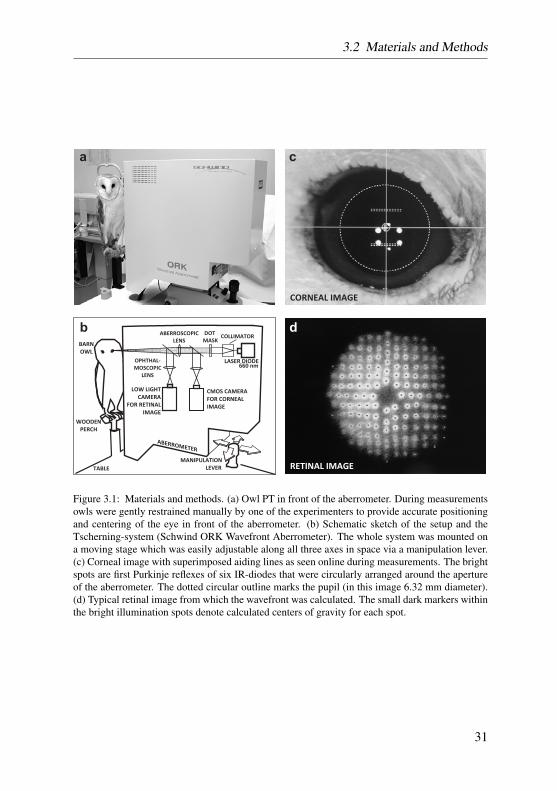
Figure 3.1: Materials and methods. (a) Owl PT in front of the aberrometer. During measurementsowls were gently restrained manually by one of the experimenters to provide accurate positioningand centering of the eye in front of the aberrometer. (b) Schematic sketch of the setup and theTscherning-system (Schwind ORK Wavefront Aberrometer). The whole system was mounted ona moving stage which was easily adjustable along all three axes in space via a manipulation lever.(c) Corneal image with superimposed aiding lines as seen online during measurements. The brightspots are first Purkinje reflexes of six IR-diodes that were circularly arranged around the apertureof the aberrometer. The dotted circular outline marks the pupil (in this image 6.32 mm diameter).(d) Typical retinal image from which the wavefront was calculated. The small dark markers withinthe bright illumination spots denote calculated centers of gravity for each spot.
31
3 Ocular aberrations
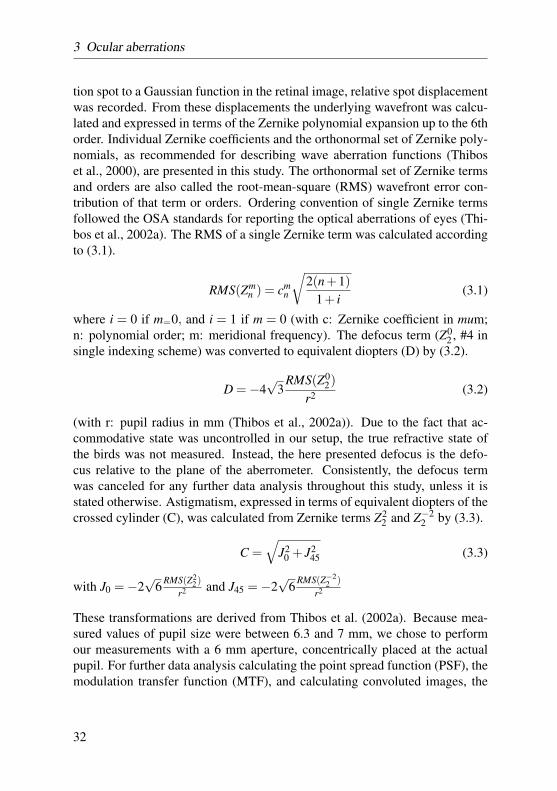
tion spot to a Gaussian function in the retinal image, relative spot displacementwas recorded. From these displacements the underlying wavefront was calcu-lated and expressed in terms of the Zernike polynomial expansion up to the 6thorder. Individual Zernike coefficients and the orthonormal set of Zernike poly-nomials, as recommended for describing wave aberration functions (Thiboset al., 2000), are presented in this study. The orthonormal set of Zernike termsand orders are also called the root-mean-square (RMS) wavefront error con-tribution of that term or orders. Ordering convention of single Zernike termsfollowed the OSA standards for reporting the optical aberrations of eyes (Thi-bos et al., 2002a). The RMS of a single Zernike term was calculated accordingto (3.1).
RMS(Zmn ) = cm
n
√2(n+1)
1+ i(3.1)
where i = 0 if m=0, and i = 1 if m = 0 (with c: Zernike coefficient in mum;n: polynomial order; m: meridional frequency). The defocus term (Z0
2 , #4 insingle indexing scheme) was converted to equivalent diopters (D) by (3.2).
D =−4√
3RMS(Z0
2)r2 (3.2)
(with r: pupil radius in mm (Thibos et al., 2002a)). Due to the fact that ac-commodative state was uncontrolled in our setup, the true refractive state ofthe birds was not measured. Instead, the here presented defocus is the defo-cus relative to the plane of the aberrometer. Consistently, the defocus termwas canceled for any further data analysis throughout this study, unless it isstated otherwise. Astigmatism, expressed in terms of equivalent diopters of thecrossed cylinder (C), was calculated from Zernike terms Z2
2 and Z−22 by (3.3).
C =√
J20 + J2
45 (3.3)
with J0 =−2√
6 RMS(Z22 )
r2 and J45 =−2√
6 RMS(Z−22 )
r2
These transformations are derived from Thibos et al. (2002a). Because mea-sured values of pupil size were between 6.3 and 7 mm, we chose to performour measurements with a 6 mm aperture, concentrically placed at the actualpupil. For further data analysis calculating the point spread function (PSF), themodulation transfer function (MTF), and calculating convoluted images, the
32
3.3 Results
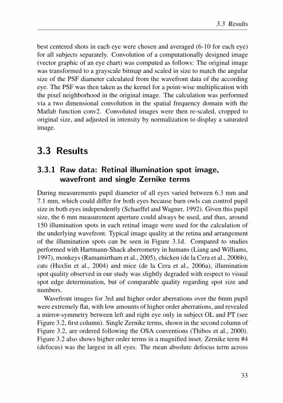
best centered shots in each eye were chosen and averaged (6-10 for each eye)for all subjects separately. Convolution of a computationally designed image(vector graphic of an eye chart) was computed as follows: The original imagewas transformed to a grayscale bitmap and scaled in size to match the angularsize of the PSF diameter calculated from the wavefront data of the accordingeye. The PSF was then taken as the kernel for a point-wise multiplication withthe pixel neighborhood in the original image. The calculation was performedvia a two dimensional convolution in the spatial frequency domain with theMatlab function conv2. Convoluted images were then re-scaled, cropped tooriginal size, and adjusted in intensity by normalization to display a saturatedimage.
3.3 Results
3.3.1 Raw data: Retinal illumination spot image,wavefront and single Zernike terms
During measurements pupil diameter of all eyes varied between 6.3 mm and7.1 mm, which could differ for both eyes because barn owls can control pupilsize in both eyes independently (Schaeffel and Wagner, 1992). Given this pupilsize, the 6 mm measurement aperture could always be used, and thus, around150 illumination spots in each retinal image were used for the calculation ofthe underlying wavefront. Typical image quality at the retina and arrangementof the illumination spots can be seen in Figure 3.1d. Compared to studiesperformed with Hartmann-Shack aberrometry in humans (Liang and Williams,1997), monkeys (Ramamirtham et al., 2005), chicken (de la Cera et al., 2006b),cats (Huxlin et al., 2004) and mice (de la Cera et al., 2006a), illuminationspot quality observed in our study was slightly degraded with respect to visualspot edge determination, but of comparable quality regarding spot size andnumbers.
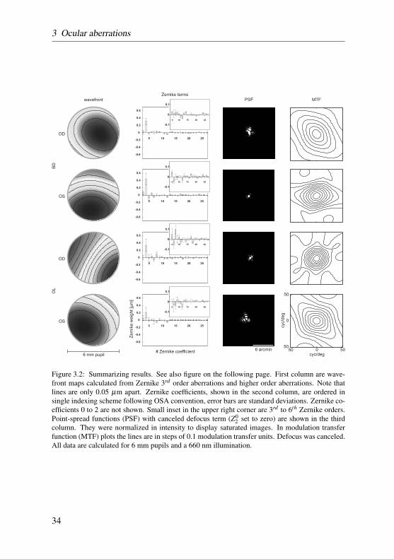
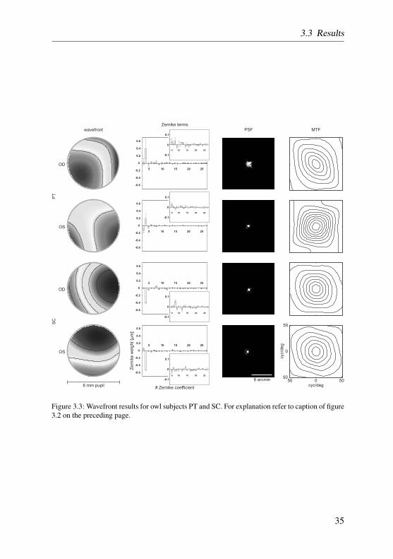
Wavefront images for 3rd and higher order aberrations over the 6mm pupilwere extremely flat, with low amounts of higher order aberrations, and revealeda mirror-symmetry between left and right eye only in subject OL and PT (seeFigure 3.2, first column). Single Zernike terms, shown in the second column ofFigure 3.2, are ordered following the OSA conventions (Thibos et al., 2000).Figure 3.2 also shows higher order terms in a magnified inset. Zernike term #4(defocus) was the largest in all eyes. The mean absolute defocus term across
33
3 Ocular aberrations
5 10 15 20 25
-0.6
-0.4
-0.2
0
0.2
0.4
0.6
5 10 15 20 25
-0.6
-0.4
-0.2
0
0.2
0.4
0.6
5 10 15 20 25
-0.6
-0.4
-0.2
0
0.2
0.4
0.6
BD
OL
OD
OS
OD
OS
wavefront
Zernike termsPSF MTF
# Zernike coefficient
Ze
rnik
ew
eig
ht
[µm
]
6 mm pupil0 50
0
50
5050
cyc/deg
cyc/d
eg
6 arcmin
5 10 15 20 25
-0.6
-0.4
-0.2
0
0.2
0.4
0.6
0.1
0
-0.1
106 15 20 25
0.1
0
-0.1
106 15 20 25
0.1
0
-0.1
106 15 20 25
0.1
0
-0.1
106 15 20 25
Figure 3.2: Summarizing results. See also figure on the following page. First column are wave-front maps calculated from Zernike 3rd order aberrations and higher order aberrations. Note thatlines are only 0.05 µm apart. Zernike coefficients, shown in the second column, are ordered insingle indexing scheme following OSA convention, error bars are standard deviations. Zernike co-efficients 0 to 2 are not shown. Small inset in the upper right corner are 3rd to 6th Zernike orders.Point-spread functions (PSF) with canceled defocus term (Z0
2 set to zero) are shown in the thirdcolumn. They were normalized in intensity to display saturated images. In modulation transferfunction (MTF) plots the lines are in steps of 0.1 modulation transfer units. Defocus was canceled.All data are calculated for 6 mm pupils and a 660 nm illumination.
34
3.3 Results
5 10 15 20 25
-0.6
-0.4
-0.2
0
0.2
0.4
0.6
5 10 15 20 25
-0.6
-0.4
-0.2
0
0.2
0.4
0.6
5 10 15 20 25
-0.6
-0.4
-0.2
0
0.2
0.4
0.6
5 10 15 20 25
-0.6
-0.4
-0.2
0
0.2
0.4
0.6
PT
SC
OD
OS
OD
OS
wavefront
Zernike termsPSF MTF
# Zernike coefficient
Ze
rnik
ew
eig
ht
[µm
]
6 mm pupil0 50
0
50
5050
cyc/deg
cyc/d
eg
6 arcmin
0.1
0
-0.1
106 15 20 25
0.1
0
-0.1
106 15 20 25
0.1
0
-0.1
106 15 20 25
0.1
0
-0.1
106 15 20 25
Figure 3.3: Wavefront results for owl subjects PT and SC. For explanation refer to caption of figure3.2 on the preceding page.
35
3 Ocular aberrations
all subjects was 0.35 µm (STD: 0.11 µm), while the mean of absolute higherorder terms was 0.012 µm (STD: 0.017 µm) across all subjects. Expressedin this way, the defocus term accounted for 96.6 % of all aberrations (2nd to6th order) across all subjects. Aberrations up to the 6th order were present butcontributed only in a minor fashion to total wavefront error.
3.3.2 Second-order aberrations
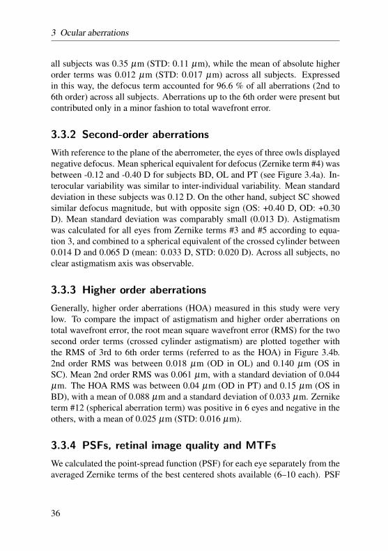
With reference to the plane of the aberrometer, the eyes of three owls displayednegative defocus. Mean spherical equivalent for defocus (Zernike term #4) wasbetween -0.12 and -0.40 D for subjects BD, OL and PT (see Figure 3.4a). In-terocular variability was similar to inter-individual variability. Mean standarddeviation in these subjects was 0.12 D. On the other hand, subject SC showedsimilar defocus magnitude, but with opposite sign (OS: +0.40 D, OD: +0.30D). Mean standard deviation was comparably small (0.013 D). Astigmatismwas calculated for all eyes from Zernike terms #3 and #5 according to equa-tion 3, and combined to a spherical equivalent of the crossed cylinder between0.014 D and 0.065 D (mean: 0.033 D, STD: 0.020 D). Across all subjects, noclear astigmatism axis was observable.
3.3.3 Higher order aberrations
Generally, higher order aberrations (HOA) measured in this study were verylow. To compare the impact of astigmatism and higher order aberrations ontotal wavefront error, the root mean square wavefront error (RMS) for the twosecond order terms (crossed cylinder astigmatism) are plotted together withthe RMS of 3rd to 6th order terms (referred to as the HOA) in Figure 3.4b.2nd order RMS was between 0.018 µm (OD in OL) and 0.140 µm (OS inSC). Mean 2nd order RMS was 0.061 µm, with a standard deviation of 0.044µm. The HOA RMS was between 0.04 µm (OD in PT) and 0.15 µm (OS inBD), with a mean of 0.088 µm and a standard deviation of 0.033 µm. Zerniketerm #12 (spherical aberration term) was positive in 6 eyes and negative in theothers, with a mean of 0.025 µm (STD: 0.016 µm).
3.3.4 PSFs, retinal image quality and MTFs
We calculated the point-spread function (PSF) for each eye separately from theaveraged Zernike terms of the best centered shots available (6–10 each). PSF
36
3.3 Results
0.2
0.4
0.6
de
focu
ssp
he
rica
le
qu
iva
len
t[D
]
astig
ma
stis
msp
he
rica
le
qu
iva
len
t[D
]
ODOD
astigmatism
defocus
RM
S[µ
m]
0.05
0.10
0.15
0.20HOA (3 to 6 order)
astigmatism
rd th
a bBDBD OLOL PTPT SCSC
owl subjectowl subject
100
75
50
25
x103-
OSOS
Figure 3.4: (a) Defocus and astigmatism. Spherical error derived from Zernike term Z02 (defocus)
and terms Z22 and Z−2
2 (astigmatism, crossed cylinder) expressed in units of spherical equivalent inall subjects and eyes. Error bars denote standard deviations across measurements. Note the twodifferent ordinates for defocus and astigmatism. (b) Lower and higher order aberrations. The 2nd
order RMS (without defocus) is plotted together with 3rd to 6th order RMS (HOA) for each eye inall animals. Error bars denote standard deviations across measurements.
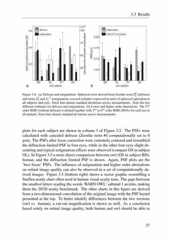
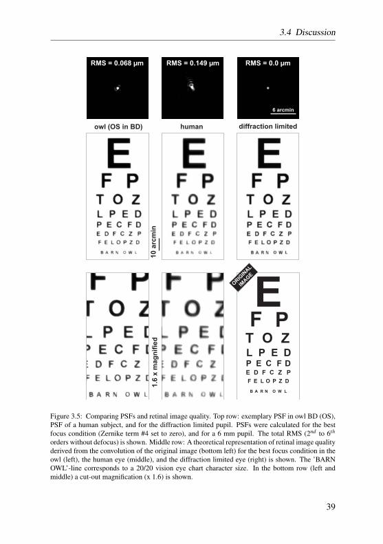
plots for each subject are shown in column 3 of Figure 3.2. The PSFs werecalculated with canceled defocus (Zernike term #4 computationally set to 0µm). The PSFs after focus correction were extremely centered and resembledthe diffraction limited PSF in four eyes, while in the other four eyes slight de-centring and typical astigmatism effects were observed (compare OS in subjectOL). In Figure 3.5 a more direct comparison between owl (OS in subject BD),human, and the diffraction limited PSF is shown. Again, PSF plots are the’best focus’ PSFs. The influence of astigmatism and higher order aberrationson retinal image quality can also be observed in a set of computationally de-rived images. Figure 3.5 (bottom right) shows a vector graphic resembling aSnellen acuity chart often used in human visual acuity tests. The gaps betweenthe smallest letters reading the words ’BARN OWL’ subtend 1 arcmin, makingthem the 20/20 acuity benchmark. The other charts in this figure are derivedfrom a two-dimensional convolution of the original image with the PSF kernelpresented at the top. To better identify differences between the two versions(owl vs. human), a cut-out magnification is shown as well. As a conclusionbased solely on retinal image quality, both human and owl should be able to
37
3 Ocular aberrations
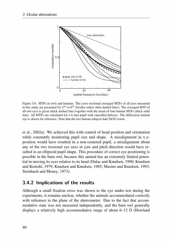
identify the smallest letters presented in this chart.The complete two-dimensional modulation transfer functions (MTFs) for the
6 mm pupil of all eyes are plotted in the rightmost column of Figure 3.2 (2nd to6th orders, defocus term canceled). Two radial cross-sections (x and y directionof Figure 3.2) of the MTF for all eyes are averaged and plotted in Figure 3.6(thin dashed lines). The diffraction limited 6 mm pupil is plotted for referenceas well. For comparison, the mean MTF of all owl eyes are plotted togetherwith the mean MTF of two human subjects which participated in this study aswell (pupil size was scaled to 6 mm with a re-converted Taylor polynomial).Again, only the defocus-corrected condition is shown. Note that the two humansubjects had 20/20 vision. Both human and owl mean modulation transfers(MTs) are almost identical across all spatial frequencies. The owl MT exceedshuman MT slightly below 20 cyc/deg and falls short of human MT above 30cyc/deg.
3.4 Discussion
3.4.1 Methods
To our best knowledge, the here presented data is the first animal eye wavefront-error study carried out with a Tscherning-type wavefront sensor (TTWS). In re-cent publications of wavefront measurements in different animals the Hartmann-Shack sensor (HSS) is used most frequently (de la Cera et al., 2006a,b; Huxlinet al., 2004; Ramamirtham et al., 2005, 2003; Thibos et al., 2002b). Nonethe-less, results from TTWSs are of comparable acuity and reproducibility (Mrochenet al., 2000), especially when larger pupils are measured, because the typicallower spatial resolution in TTWS becomes negligible with larger pupil area.Throughout the literature several examples for the use of TTWS can be found(Jahnke et al., 2006; Kaemmerer et al., 2000; Krueger et al., 2001; Mierdelet al., 1997, 2001; Mrochen et al., 2000, 2003; Prieto et al., 2000). Generally,benefits from the use of TTWSs are that the ingoing light path is used for mea-surement and that the illumination light source lies in the visible part of thespectrum. HSSs are more frequently used in state-of-the-art wavefront mea-surement applications, because they are less sensitive to scattering, and usuallyperform at higher resolution.
One of the key requirements in wavefront analysis is the alignment of thesubjects visual axis with the optical axis of the measurement system (Thibos
38
3.4 Discussion
owl (OS in BD) diffraction limited
6 arcmin
human
EF P
T O ZL P E DP E C F DE D F C Z P
F E L O P Z D
B A R N O W L
10
arc
min
1.6
xm
ag
nif
ied
RMS = 0.068 µm RMS = 0.149 µm RMS = 0.0 µm
ORIG
INAL
IMAGE
Figure 3.5: Comparing PSFs and retinal image quality. Top row: exemplary PSF in owl BD (OS),PSF of a human subject, and for the diffraction limited pupil. PSFs were calculated for the bestfocus condition (Zernike term #4 set to zero), and for a 6 mm pupil. The total RMS (2nd to 6th
orders without defocus) is shown. Middle row: A theoretical representation of retinal image qualityderived from the convolution of the original image (bottom left) for the best focus condition in theowl (left), the human eye (middle), and the diffraction limited eye (right) is shown. The ’BARNOWL’-line corresponds to a 20/20 vision eye chart character size. In the bottom row (left andmiddle) a cut-out magnification (x 1.6) is shown.
39
3 Ocular aberrations
zero aberration
owl (n=8)
human (n=4)
spatial frequency [cyc/deg ]
modula
tion
transfe
r
0 20 400
1
0.5
Figure 3.6: MTFs in owls and humans. The cross-sectional averaged MTFs of all eyes measuredin this study are presented for 2nd to 6th Zernike orders (thin dashed lines). The averaged MTF ofall owl eyes is given (thick dashed line) together with the mean of four human MTFs (thick solidline). All MTFs are calculated for a 6 mm pupil with cancelled defocus. The diffraction limitedeye is shown for reference. Note that the two human subjects had 20/20 vision.
et al., 2002a). We achieved this with control of head position and orientationwhile constantly monitoring pupil size and shape. A misalignment in x-y-position would have resulted in a non-centered pupil, a misalignment aboutany of the two torsional eye axes in yaw and pitch direction would have re-sulted in an ellipsoid pupil shape. This procedure of correct eye positioning ispossible in the barn owl, because this animal has an extremely limited poten-tial in moving its eyes relative to its head (Dulac and Knudsen, 1990; Knudsenand Konishi, 1979; Knudsen and Knudsen, 1985; Masino and Knudsen, 1993;Steinbach and Money, 1973).
3.4.2 Implications of the results
Although a small fixation cross was shown to the eye under test during theexperiments, it remains unclear, whether the animals accommodated correctlywith reference to the plane of the aberrometer. Due to the fact that accom-modative state was not measured independently, and the barn owl generallydisplays a relatively high accommodative range of about 6–12 D (Howland
40
3.4 Discussion
et al., 1991; Schaeffel and Wagner, 1992), the here measured relative defocuswas omitted from further analysis. Without drawing conclusions about normaldefocus from our data, results from an earlier developmental study in barn owlsshowed, that refractive errors larger than 1 D disappeared during the first twoweeks of juvenile development in this animal (Schaeffel and Wagner, 1996).
Despite the uncertainty of the true amount and sign of defocus in barn owleyes, all animals show little amounts of astigmatism and very little higher or-der aberrations. Typical values of HOA in humans are about 3.3 times largerthan HOA reported here (Howland, 2002; Porter et al., 2001). Also, HOAin eyes of another nocturnal species, the cat, are about 3.7 times larger thanthose of the owl (Huxlin et al., 2004). While HOA are lower in the barn owlcompared to those in human eyes in an absolute sense, this difference might be-come even more prominent when put into relation with absolute eye size. Axiallength of barn owl eyes is about 3/4 of that of human eyes (17.5 vs. 24.5 mm,(Hughes, 1977; Schaeffel and Wagner, 1996)), and following an observationby Howland, with the same set of optics and pupil size, the wave aberrations inthe smaller eye should be larger than in the bigger one (Howland, 2005). Wealso showed typical PSFs of the owl eye and compared it to that derived fromone human subject. Convoluted images revealed that theoretical retinal im-age quality is comparable in man and owl (compare also Artal (1990)). Meanmodulation transfer of all tested owl eyes almost exactly matched modulationtransfer in the two human subjects we included in this study. Taken together,the data presented here show that averaged retinal image quality in the eyes ofbarn owls is excellent.
Nevertheless, based on retinal ganglion cell counts, barn owls show onlypoor grating acuity of about 7.8 cyc/deg (Oehme, 1961; Wathey and Pettigrew,1989). This finding is supported by a pattern electro-retinogram study whichcalculates grating acuity to be 6.98 cyc/deg in the barn owl (Ghim and Hodos,2006). The question arising from these findings is why the optics of the owl’seye would have evolved in a fashion allowing the formation of a retinal imagewith a quality that is far beyond a visual acuity given by the neural compo-nents creating vision in this bird. A similar question has been discussed in arecent study measuring the optical quality in cat eyes (Huxlin et al., 2004). Theauthors propose that given the nocturnal lifestyle of the cat combined with analmost three times larger pupil area in cats compared to humans at the samelight levels, cats should experience significantly more optical interference thanhumans at the same light level. The authors conclude that the cat’s optics arerelatively good because otherwise additional aberrations would degrade vision
41
3 Ocular aberrations
to levels of unsustainability (Huxlin et al., 2004). Given the relatively lowhigh-frequency visual acuity in the barn owl (below 10 cyc/deg), this argu-ment might not stand up to a quantitative analysis. On the other hand, beingequipped with excellent optics that raise the MTF over all spatial frequencies,the owl might take advantage from an elevated contrast sensitivity for low spa-tial frequencies close to its neural sample pattern (compare Figure 3.6). Thus,while flying in the dark, owls might better manoeuvre through and avoid hit-ting low spatial frequency objects like e.g. limbs of a tree, and better visuallyidentify items of prey. As an example, a mouse (6 cm) viewed from typicalstriking distance (5 m) would subtend about 0.7 cyc/deg, which matches theowl’s contrast sensitivity function peak quite well (Ghim and Hodos, 2006).
42
3.4 Discussion
43
3 Ocular aberrations
44
4 Spatial contrast sensitivity
Abstract
In this study a psychophysical approach measuring the spatial contrast sensitivity function (CSF)in the visual system of the barn owl (Tyto alba pratincola) is presented. Contrast sensitivity wasmeasured in a two-alternative forced choice orientation discrimination task. Gaussian filtered si-nusoidal gratings were used as stimuli. During a single experimental session, spatial frequencywas held constant while contrast was varied, following a two-down one-up staircase procedure.The CSF found here renders the typical band-limited, inverted u-shaped function reported for a setof species in other studies. Maximal sensitivity was found at a spatial frequency of 1.01 cyc/deg.At this spatial frequency, contrast discrimination threshold was about 0.06, or, in terms of con-trast sensitivity, about 18. Grating acuity was estimated from the CSF high frequency cut-offand yielded 3.8 cyc/deg. In a second experiment in which contrast was held constant and spatialfrequency was varied, grating acuity was measured directly (3.6 cyc/deg). Compared to electro-physiological results, maximal contrast sensitivity found in the present study was increased by afactor of two. Compared to anatomical and electrophysiological estimates, grating acuity valueswere, on the other hand, reduced by the same factor.
45
4 Spatial contrast sensitivity
4.1 Introduction
Successful interaction with the environment requires knowledge about it. Invision, information is largely mediated by light that is reflected from the sur-faces of objects that form the environment. One feature that makes objects dis-tinguishable is the amount of luminance that is reflected relative to the back-ground or other objects. This relative luminance difference is referred to asluminance-contrast. Contrast is one of the important visual feature that makeobservers recognize their surroundings.
The spatial contrast sensitivity function (CSF) is, therefore, one of the fun-damental functional descriptions of a visual system. It relates the ability of anobserver to visually detect spatial gratings of different spatial frequencies tothe amount of luminance-contrast present. If measured behaviorally, the CSFincorporates visual functions of both physical (i.e. the visual transfer functionof the eye) and, to a greater extent, physiological nature (i.e. visual processingin the nervous system of the observer). The CSF may, therefore, be regardedas a direct measure of the perceptual high-level process of seeing.
Campbell and Green (1965b) were the first to measure the CSF in the hu-man visual system, emphasizing the importance of visual processing for ob-jects larger than the resolution limit. Apart from humans, the CSF has beenmeasured in animals of different taxa with various psychophysical techniques.Among those are macaques (de Valois et al., 1974), squirrel monkeys (Meri-gan, 1976), owl monkeys (Jacobs, 1977), bush babies (Langston et al., 1986),cats (Blake et al., 1974; Bisti and Maffei, 1974), rats (Birch and Jacobs, 1979),ground squirrels (Jacobs et al., 1980), tree shrews (Petry et al., 1984), wallabies(Hemmi and Mark, 1998), goldfish (Northmore and Dvorak, 1979), pigeons(Nye, 1968), eagles (Reymond, 1985), and kestrels (Hirsch, 1982). In virtu-ally all animals tested so far, the CSF renders, as in humans, a band-limited,inverted u-shaped function (Uhlrich et al., 1981). Sensitivity is best at inter-mediate spatial frequencies and is reduced at both higher and lower spatialfrequencies. The high frequency roll-off in humans is regarded as a combinedconsequence of physical constraints leading to optical degradation (such asthe diffraction limit and wave aberrations), and receptor cell spacing on retinalevel (Campbell and Green, 1965a; Cornsweet, 1970). The low frequency at-tenuation can be explained solely by neural factors, such as extent of lateralinhibition (Cornsweet, 1970), antagonistic surround mechanisms (Westheimer,1972), or relative insensitivity of low spatial frequency filters (Graham, 1972).
46
4.2 Materials and Methods
Here, we present a psychophysical measure of spatial contrast sensitivity inthe visual system of the barn owl. The barn owl is a highly specialized animal.Their visual capabilities have been demonstrated in several behavioral, physi-ological, and anatomical studies. Its prominent large eyes, being almost twiceas long as allometry based on body weight would suggest (Howland et al.,2004), are oriented frontally, and, thus, create an unusual large binocular fieldof view (Martin, 1984). These eyes have excellent optical quality (Schaeffeland Wagner, 1996), showing only one third the amount of higher order aberra-tions found in human eyes (refer to chapter 3 vs. Howland (2002)). Barn owlscan discriminate random dot stereograms with hyperacute precision (van derWilligen et al., 1998, 2002), a finding accompanied by several physiologicalstudies demonstrating a high degree of binocular interaction and selectivity inthe visual Wulst of these birds (Pettigrew and Konishi, 1976; Wagner and Frost,1993, 1994). Barn owls, similar to humans, can discriminate vernier targets ona hyperacute level when viewing with one eye alone (chapter 5). Barn owlsare distracted by crowded stimuli similar as humans are (Barrett et al., 1999;Malania et al., 2007), and show binocular summation ratios of similar magni-tude (Banton and Levi, 1991). Barn owls also do perceive illusionary contours(Nieder and Wagner, 1999). A recent study shed light on the attentional mech-anisms of vision in this bird (Ohayon et al., 2008), and suggested a top-downmodulation of gaze control when owls view natural targets.
Yet having this set of interesting and diverse approaches to barn owl visionat hand, there are only two studies dealing with the underlying basic propertiesof spatial vision in this bird. Barn owl visual acuity has been estimated byganglion-cell density (Wathey and Pettigrew, 1989), and contrast sensitivitywas recorded in a pattern electro-retinogram (PERG) study (Ghim and Hodos,2006). To be able to relate the above mentioned results to the basic features ofthe barn owl’s visual system more directly, we measured the barn owl’s contrastsensitivity function and its grating acuity in a set of behavioral experiments.
4.2 Materials and Methods
4.2.1 Subjects
The experimental animal was one male adult barn owl (Tyto alba pratincola,subject SL), taken from the institute’s breeding stock. The owl was hand-raisedand tame. Its body weight was maintained at about 90% of its free feeding
47
4 Spatial contrast sensitivity
weight. Water was given ad libitum. It was given food (chick meat) only inthe experimental booth via a food dispenser or as a reward directly after theexperiment inside the lab. Training and experiments took place on 5 days perweek. When no experiment was carried out the owl was fed in its aviary. Careand treatment of the subject was carried out in accordance with the guidelinesfor animal experimentation as approved by the ”Landesprasidium fur Natur,Umwelt und Verbraucherschutz Nordrhein Westfalen”, Recklinghausen, Ger-many, and complied with the ”NIH Guide for the use and care of laboratoryanimals”.
4.2.2 Experimental setup and stimuli
All experiments were conducted in a sound and light proof chamber, with noadditional light source other than the stimulus display. The owl was sitting ona wooden perch in front of two response keys that were symmetrically placedleft and right to an automated food dispenser. Its head was unrestrained and,upon the onset of a trial, oriented fronto-parallel relative to the stimulus display.Viewing distance was 85 cm, making one pixel subtend 1.044 arcmin of visualangle (figure 4.1).
The stimuli were gaussian filtered sinusoidal gratings (Gabor patch) of twodiscrete axes of orientation. The sinusoidal function propagated either in 0°or 90° direction relative to the coordinate system of the display (horizontal orvertical orientation, respectively, see figure 4.1). The standard deviation of theGaussian was held constant at 0.48 while the phase of the sinusoid was alteredtrial-by-trial randomly in a 180° interval (not in training sessions). The Ga-bor patch, 12.2 degree of visual angle in diameter, was shown centered on thescreen when a trial was initiated. The rest of the display was filled with an uni-form gray surface. The whole screen was covered with a large sheet of linearneutral density filter (Lee Filter) that lowered overall luminance by approx-imately one log unit, producing a mean luminance of 2.741 cd/m2, equallydistributed at the whole Gabor patch area. Stimulus contrast was controlledby modification of the amplitude of the sinusoid and measured at viewing dis-tance in a pre-experimental calibration sequence with the Minolta LS-100. Ourdisplay system was able to produce stimulus contrasts ranging from 0.991 to0.0092 reliably. Contrast is defined throughout this study according to theMichelson-formula: contrast = (lummax − lummin)/(lummax + lummin). Thechoice of spatial frequencies used in the training sessions and experiments wasaccording to results from pilot testing and earlier studies with the same animal
48
4.2 Materials and Methods
VD
85cm
Figure 4.1: A sketch of an inside view of the experimental booth, showing the relevant parts ofthe experimental setup. The barn owl was sitting on a wooden perch fixed in front of an automatedfeeder, which delivered small pieces of meat upon correct responses (F). The two response keys,corresponding to the two stimulus configurations, were in easy reach of the owls beak (L,R).Viewing distance (VD) was 85 cm. The computer display was covered with a linear neutral densityfilter to reduce glare (ND). This picture shows the situation when the horizontal oriented Gaborpatch was shown. A small IR-camera monitored the owls gaze, which in case of a fronto-parallelorientation triggered trial progress (C). Note that under experimental conditions the room wascompletely dark.
subject and setup (chapter 5).
Visual stimulus generation was controlled by custom written software (ANSI-C with the Open-GL utility kit GLUT), running on an Apple G5 workstationwith a 8-bit graphics board (NVidia Geforce 6800 GPU), and digitally outputon a 23” Apple Cinema Display. Owl responses were recorded via a custombuilt USB-interface, hooked up to the standard computer mouse input. Thefeeder was controlled by TTL-pulses produced by a USB input/output device(BMCM, Germany).
49
4 Spatial contrast sensitivity
4.2.3 Psychophysical procedures
A small, flashing fixation target was shown in the center of the display betweentrials to attract the owl’s gaze and to support correct orientation. When thesubject oriented its gaze toward the screen, a trial was initiated and the stimuluswas shown. After stimulus onset the owl had to peck one of two response keys,with the left key corresponding to a horizontal oriented grating and the rightkey to the vertical orientation. Horizontal or vertical gratings were presentedin a pseudo-random order. That is, no more than three repetitions of one ofthe two alternatives were presented consecutively. The owl was rewarded afterevery correct response, false responses were not punished. The time course wasself-paced to allow the owl an exact observation of the stimulus. Whenever theowl made large head movements and stopped fixating the display, the trial wasaborted.
The owl was extensively trained to discriminate the two different gaborpatches correctly before experiments began. During this training phase thestimulus contrast, its spatial frequency, and the phase position of the sinusoidwas held constant (contrast: 0.991, spatial frequency: 0.61 cyc/deg, phase:90°). We termed the performance level in the training task as being signif-icant and moved on to the experimental phase, when the owl’s performancelay above the 99 % confidence interval of a binomial process performing atchance level. As an example, in an experiment consisting 100 trials, significantperformance was given if at least 63 correct responses were observed.
After the training phase and prior to contrast sensitivity experiments, severalcontrol experiments were conducted. First, we altered the pseudo-random de-sign of the trial sequence to allow up to 7 repetitions of one alternative consecu-tively. This control intended to rule out strategy learning in the subject, makinghim, at low stimulus intensities, guessing better than chance level. Secondly,we wanted to find out whether the owl had incorporated a perceptual stable con-cept of the visual feature that had to be discriminated, and responded accordingto orientation only. Therefore, we presented Gabor patches with (a) sinusoidsof random phase, (b) three spatial frequencies not shown during training (atfixed ratios 1.5, 0.75, and 0.5 fold the training wavelength), and (c) randomspatial frequencies drawn from an even larger interval.
Typically, a single experimental session consisted of about 70 to 100 trials.Every experimental session was conducted at a single spatial frequency. Stim-ulus intensity choice within a session followed a simple up-down transformedrule. That is, stimulus intensity (i.e. contrast) was decreased after two consec-
50
4.2 Materials and Methods
utive correct responses and was increased after every false response. In thisway, converging to stimulus intensities at which the animal responded 70.7 %of the time correctly, the choice of stimulus intensities presented to the animallay near the threshold. To prevent a quick fatigue and frustration of the owl,bonus trials at high stimulus intensities were given from time to time. Theeleven spatial frequencies used in our experiments ranged from 0.38 to 2.17cyc/deg, and, thus, covered about 2.5 octaves of the spectrum. The differentspatial frequencies were applied in an iterative order. That is, we started witha high spatial frequency, moved on to a low spatial frequency, followed by anintermediate spatial frequency and so on.
For further analysis, the results of two consecutive experimental sessionsat each spatial frequency were combined to build the basis of psychophysicalraw data (see figure 4.2 for an example). This was done by re-calculatingthe performance level at each stimulus intensity from the pooled data of bothruns. This procedure balanced out inconsistencies in performance that occurredon different testing days. Note that it did not necessarily produce an averagethreshold of both runs.
4.2.4 Data analysis and grating acuity
For all eleven spatial frequencies, the behavioral performance, i.e. the percent-age of correct responses, was plotted as a function of stimulus intensity. With apopular bootstrap method described by Wichmann and Hill (2001a) used in theMatlab function pfit, a logistic function Ψ(x) (4.1) was fitted to the data points,generating a complete psychometric function.
Ψ(x) = γ +(1− γ−λ )∗ 11+ e α−x
β
(4.1)
where Ψ(x) is behavioral performance at stimulus intensity x, α and β are thefit parameters. Contrast threshold was defined as the stimulus intensity on thepsychometric function half-way between lower (γ) and upper (λ ) asymptote.The lower asymptote was set to 0.5, the upper asymptote was corrected to ac-count for lapses the owl sometimes showed at high stimulus intensities. Witha statistical re-sampling of the data points (n=1000), the 95 % confidence in-tervals at threshold level were calculated (Wichmann and Hill, 2001b). Thecontrast sensitivity and its confidence interval was calculated as the inverse ofthe contrast threshold.
51
4 Spatial contrast sensitivity
0.01 0.1 1
0.4
0.5
0.6
0.7
0.8
0.9
1
contrast
perf
orm
ance
1.52 cyc/deg
CS = 15.41 @ 72.9 %
n = 188
0.4
0.6
0.8
1
CS = 16.63
n = 94
0.01 0.1 1
0.4
0.6
0.8
1
contrast
perf
orm
ance
CS = 13.08
n = 94
a b
Figure 4.2: An example for the combination process used throughout this study. In (a) two psy-chometric functions of subsequent experimental sessions are shown. The ratio of correct responseswere defined as behavioral performance and denoted on the y-axis. In this example, spatial fre-quency was 1.52 cyc/deg. Both sessions were comprised of 94 trials each. Contrast threshold and,inversely, contrast sensitivity (CS) were calculated from fitting a logistic psychometric functionto the data, and were defined at the inflection point of that function. The horizontal bar is the95% confidence interval at threshold level. Note that trial numbers in each session are not equallydistributed over contrast intensities due to the applied staircase rule (see section 4.2.3 for explana-tion). In (b) the two sessions are combined by re-calculating the performance at each contrast levelfor the pooled data from (a). Note that the logistic function fits the data better as in (a), as is alsoreflected by the smaller confidence interval of the threshold.
The CSF was described by a double exponential function, that was fitted tocontrast sensitivity data by a method of least squares (Uhlrich et al., 1981).Grating acuity was, then, derived computationally from an extrapolation of theCSF beyond the high frequencies tested. Additionally, grating acuity was mea-sured directly in a way similar to the method described above: at two differentfixed contrast levels (0.991 and 0.779) spatial frequency was altered accordingto the transformed up-down rule. A psychometrical function was then fittedto the behavioral discrimination performance at the different levels of spatialfrequency. The grating acuity threshold was defined as the spatial frequency atthe inflection point of the corresponding psychometrical function. Confidenceintervals were calculated as stated above.
52
4.3 Results
4.3 Results
4.3.1 Training, control experiments, and response bias
The owl reached significant behavioral performance after only 13 sessions.Mean training performance was 81.96± 7.78 % correct responses in the first 15training sessions after reaching the criterion, and 89.53 ± 6.35 % correct in alltraining (or bonus) trials recorded. In 6 control sessions the phase of the Gaborpatch was applied randomly. In all of these sessions the owl responded morethan 90 % correctly (mean: 95.0 ± 1.8 %). All other control sessions wereconducted twice and fell well within the range of normal training performance.In particular, these were two times 92.1 % correct for random wavelength, 79.6% and 94.6 % correct for up to 7 repetitions (see section 4.2.3), 87.8 % and 94.8% correct for 0.5 fold training wavelength, 93.6 % and 89.6 % correct for 0.75,and 87.8 % and 91.5 % correct for 1.5 fold training wavelength.
In total, 1189 training and bonus trials, 684 control trials, and 2642 exper-imental trials were recorded. 2017 trials made up the contrast sensitivity ex-periments, the remaining 625 trials were used for grating acuity experiments.Bias was calculated for the experimental sessions as follows: by applying thebinomial distribution (with n: total number of trials, p: percentage of hori-zontal stimuli actually shown to the owl) a 95 and 99 % confidence interval(abbreviated as CI, hereafter) was calculated for each experimental condition(spatial frequency, or contrast level in the grating acuity experiments). The in-terval, therefore, reflected the number of ’horizontal’ responses (abbreviated asHR, hereafter) the owl could give without displaying a statistically significantbias. This bias analysis was applied over the whole range of stimulus intensi-ties (global bias), and for two intervals on the intensity scale separately (splitbias). One interval, defined as near threshold, was comprised of stimulus inten-sities lower than threshold and one intensity above threshold. The remainingstimulus intensities made up the ’above threshold’ interval.
For both contrast sensitivity and grating acuity experiments, no statisticalsignificant bias was observed when a 99 % confidence interval was applied.However, on the 95 % CI level, in some cases a bias was present. In the con-trast sensitivity experiments the owl displayed a global response bias in 6 outof 11 cases (at 2.17, 1.01, 0.87, 0.76, 0.61, 0.38 cyc/deg), but with no consis-tent direction of bias. That is, in 4 cases he preferred horizontal over verticalresponses, while in the other two this relation was reversed. The owl neverdisplayed bias in trials that lay above threshold, but only in the near threshold
53
4 Spatial contrast sensitivity
trials. There was only one case in which a global bias was present in the ab-sence of bias in the split condition (0.38 cyc/deg). In one case (2.03 cyc/deg),only split bias in near threshold trials was present.
In the grating acuity experiments the owl showed a response bias, generallypreferring vertical over horizontal responses. Interestingly, this bias was differ-ently distributed over the stimulus intensities for the two contrast levels tested.At maximum contrast (0.991) the owl showed no significant bias at low stim-ulus intensities near the threshold (spatial frequency ≤ 3.0 cyc/deg). Here, theCI ranged from 60 to 81 HR, while the owl chose 63 HR (n=136). At largerstimulus intensities (n=207), the owl chose 85 HR, with a CI ranging from92 to 119 HR. At the second contrast level (0.779) this relation was reversed.There was no significant bias at high stimulus intensities (HR: 49, CI: 39–56),and again a bias towards ’vertical’ responses at lower intensities (HR: 79, CI:87–112).
4.3.2 Contrast threshold estimation
In total, 11 different spatial frequencies, spanning about 2.5 octaves of thespectrum, were tested. We started with a high spatial frequency, moved on toa low spatial frequency, followed by an intermediate spatial frequency and soon. For each of the eleven wavelengths, two single experimental sessions wereconducted. The results of the two runs were combined to calculate a singlepsychometric function (see figure 4.2 for an example). Contrast sensitivity atthe given spatial frequency was derived from the inflection point of that func-tion. Mean trial number per spatial frequency was 183.4 ± 35.3 (refer to table4.1). In all combined sessions, 7 to 10 stimulus intensities were tested. Ex-cept in one case (2.0 cyc/deg) there were always at least 3 intensity steps aboveor below threshold. Mean trial numbers near the threshold (4 intensity stepscentered around threshold) were 106.3 ± 22.1. Threshold levels lay between72.5 and 75 % correct responses. Deviances from the theoretical midpoint inthe psychometrical function (75 % correct responses) appeared due to lapsecorrection at high stimulus intensities in 6 out of 11 cases (see figure 4.3 for anoverview of all eleven psychometric functions).
A maximum sensitivity of 18.87 (CI: 17.24–22.73) was found at a wave-length of 60 pixels (1.01 cyc/deg). This value corresponds to a Michelson con-trast of 0.053. With longer wavelengths, contrast sensitivity decreased mono-tonically. At the longest wavelength (160 pixels, 0.38 cyc/deg), contrast sensi-tivity dropped to 2.632 (CI: 2.320–3.367), corresponding to a contrast of 0.38.
54
4.3 Results
1.74 cyc/deg
CS = 13.33 @ 75.0 %
n = 1311.52 cyc/deg
CS = 15.38 @ 72.9 %
n = 1881.22 cyc/deg
CS = 15.63 @ 72.5 %
n = 202
1.01 cyc/deg
CS = 18.87 @ 72.5 %
n = 2630.76 cyc/deg
CS = 7.143 @ 75.0 %
n = 198
0.61 cyc/deg
CS = 4.219 @ 75.0 %
n = 1870.47 cyc/deg
CS = 3.817 @ 72.6 %
n = 1710.38 cyc/deg
CS = 2.632 @ 72.5 %
n = 201
0.87 cyc/degn = 176
0.01 0.1 1 0.01 0.1 1 0.01 0.1 1
0.01 0.1 1 0.01 0.1 1 0.01 0.1 1
0.01 0.1 1 0.01 0.1 1 0.01 0.1 1
contrast
pe
rfo
rma
nce
0.4
0.6
0.8
1
0.4
0.6
0.8
1
0.4
0.6
0.8
1
2.03 cyc/deg
CS = 7.187 @ 73.6 %
n = 154
0.01 0.1 10.01 0.1 1
0.4
0.6
0.8
1 2.17 cyc/deg
CS = 3.215 @ 75.0 %
n = 146
CS = 16.39 @ 75.0 %
Figure 4.3: Combined psychometric functions at all spatial frequencies tested (see figure 4.2 for anexample of the combination process). Behavioral performance, i.e. the ratio of correct responses,is plotted as a function of contrast level. λ is the wavelength of the sinusoid, n the number of trials,CS is contrast sensitivity at the denoted level of performance. Note that the number of trials werenot applied equally over the whole range of contrasts, but that trials near the threshold appearedmore often due to the staircase procedure (see text for explanation). The solid line is the logisticfit to the data. The horizontal line denotes the 95% confidence interval derived from bootstrappingthe original data. Note also that threshold level was defined depending on the upper asymptote,which could differ due to lapses at high contrast levels.
55
4 Spatial contrast sensitivity
Table 4.1: Contrast sensitivity (CS) values at all spatial frequencies (SF). The 95 % confidenceinterval borders (CI), number of trials, and the performance level at which threshold was definedare given as well.
Contrast sensitivity at wavelengths shorter than 60 pixels decreased monotoni-cally, reaching the minimal sensitivity of 3.215 (CI: 2.040–4.291) at 28 pixels.Here, threshold contrast was 0.31.
4.3.3 Contrast sensitivity function
Contrast sensitivity values derived from the combined experimental sessionswere plotted against spatial frequency on a double logarithmic scale (see fig-ure 4.4). Sensitivity values increased strictly monotonic from low spatial fre-quencies up to intermediate spatial frequencies, where sensitivity was maximal(18.87 at 1.01 cyc/deg). Consistently, going further to higher spatial frequen-cies, sensitivity decreased strictly monotonic. A double exponential function(4.2) was fitted to the normalized data by a method of least squares. Thisfour-parameter function was found to provide a good fit to the CSF of severalspecies (Uhlrich et al., 1981).
S(γ) = 100(K1e−2παγ −K2e−2πβγ) (4.2)
where S(γ) is contrast sensitivity at spatial frequency γ . Our best fit wasfound for the following parameters: K1 = 1.536, K2 = 1.562, α = 0.2489,β = 0.2556. Peak sensitivity derived from this function was 13.91 at a spatialfrequency of 0.963 cyc/deg. The width of the CSF was measured in octaves as
56
4.3 Results
1.0 60.2
1
10
20
spatial frequency [cyc/deg]
contr
astsensitiv
ity
Figure 4.4: The contrast sensitivity function in the barn owl visual system. Contrast sensitivitywas defined as the inverse of contrast thresholds and was plotted against spatial frequency. Thedark circles are the sensitivity values derived from combination of two consecutive experimentalsessions. The thresholds resulting from the single sessions are plotted in gray. The vertical barsare the 95 % confidence intervals calculated from the combined psychometric functions (see figure4.3). The sensitivity values were fitted to a double exponential function by a method of least-squares (solid line). The two thresholds found in the grating acuity experiments are drawn forreference as well (bottom right). The dotted line connects contrast sensitivity thresholds and isdrawn for pictorial purposes only.
the distance between the spatial frequency on either side of the peak frequencyat which sensitivity declined by a factor of two. That is, width at half amplitudewas 2.69 octaves (0.45–2.90 cyc/deg). The high frequency cut-off (S(γ) = 1)was 3.81 cyc/deg.
4.3.4 Grating acuity
Grating acuity was measured at two contrast levels (0.991 and 0.779) witha method similar to the one used in the contrast sensitivity experiments andwith identical stimulus configuration. In total, 343 trials in 4 experimentalsessions were recorded at maximum contrast. Grating acuity, expressed asthe wavelength of the sinusoid at which discrimination performance was atthreshold, was at both contrast levels similar: at 0.991 contrast level, grating
57
4 Spatial contrast sensitivity
6.1 3.0 2.0 1.5 1.2 1.0 0.9
0.4
0.5
0.6
0.7
0.8
0.9
1
spatial frequency [cyc/deg]
pe
rfo
rma
nce
6.1 3.0 2.0 1.5
5050
1010
2525
0.4
0.5
0.6
0.7
0.8
0.9
1
spatial frequency [cyc/deg]
pe
rfo
rma
nce
trials
trials
contrast: 0.991 contrast: 0.779n=343 n=282
GA = 3.51 @ 75.0 %GA = 3.62 @ 72.5 %
Figure 4.5: Grating acuity was measured at two contrast levels. The left panel shows the results atthe highest contrast level possible with our display system (0.991). The circles denote discrimina-tion performance at a given wavelength of the Gabor patch presented. The solid line is the logisticfit to the data, the small horizontal bar is the 95 % confidence interval at threshold (Wichmann andHill, 2001a,b). At maximum contrast, 343 trials were recorded, with the majority lying aroundthreshold level (see bar plot at the bottom of each panel, denoting trial numbers per stimulus in-tensity). Grating acuity threshold was found at a wavelength of 16.78 pixels, equalling a spatialfrequency of 3.62 cyc/deg. Due to lapses the owl displayed at high stimulus intensities, the up-per asymptote of the psychometric function was corrected. In the right panel, the results for the0.779 contrast level are shown. In total, 282 trials were recorded, grating acuity was at 17.36 pix-els, equalling 3.51 cyc/deg. Note that in the condition shown in the right panel, additional spatialfrequencies (1.0, 0.7, 0.6 cyc/deg) were tested and lead to 100% correct responses. For figuralpurposes, these are not shown here.
acuity was 16.78 pixels (CI: 12.86–18.36 pixels). This value equals a spatialfrequency of 3.62 cyc/deg. Here, performance level at threshold was 72.5 %correct responses, due to lapses at high stimulus intensities. Out of the 343trials, the 7 smallest intensity steps (12, 14, 15, 16, 18, 20, 25 pixel) madeup about 60 percent of all trials. This was due to the staircase rule applied tostimulus intensity choice (compare figure 4.5).
In the lower contrast condition (0.779) grating acuity was 17.36 pixels (CI:15.98–18.30 pixels), or 3.51 cyc/deg, defined at 75.0 % correct response level.Here, out of 282 trials recorded in 3 sessions, 202 trials (71.6 %) were recordednear threshold level (12, 14, 15, 16, 17, 18, 20 pixels).
58
4.4 Discussion
4.4 Discussion
4.4.1 Methodological considerations
Presenting acute contrast defined stimuli on a LCD computer display is the-oretically limited in at least two ways: First, the minimal luminance-contrastpossible to be displayed might be not suited for extreme low-contrast stimuli.We measured the actual contrast at every amplitude-step used in the experi-ments with the Minolta LS-100 luminance meter in a calibration sequence. Thesystem was able to present contrasts below 0.01 reliably, and since all discrim-ination thresholds found in the experiments were at contrasts above 0.05, thedisplay was suited for our purposes. Second, due to only 256 grayscale levelspossible to be output by the graphics-card, at low contrasts and/or low spatialfrequencies, the system might introduce unwanted high frequency borders inthe intended sinusoidal signal. The stimulus, then, would appear ”jagged” andnot smooth. We tested this psychophysically with a human observer, reportingthe jaggedness of the stimulus. Again, aliasing artifacts appeared only at con-trasts below 0.01, lying clearly beyond the range of contrasts actually tested inthe experiments. We concluded from this, that our display system, while in-appropriate for human observers, was suitable for contrast thresholding in thecomparably limited range given by the visual system of the barn owl. This no-tion was also reflected by the low-frequency roll-off displayed in the actuallymeasured contrast sensitivity function.
4.4.2 Implications of the results
Based on the results of the control experiments, we conclude that the owl wasable to incorporate a concept of the task, making a decision based on the orien-tation of the grating in the Gabor patch alone, a prerequisite for the use of theorientation discrimination paradigm. In trials with gratings of spatial frequen-cies that were never used in the training sessions before, the owl showed similarperformance as in the training sessions. This was also true when the gratingwas presented with random phase configuration. Moreover, the responses tothe stimulus showed robustness against a change in inter-trial alternative choiceto a quite large extent. While in training trials no more than three repetitionsof one alternative occurred consecutively, this was changed to a maximum of7 possible consecutive repetitions in the control sessions. Again, performancedid not drop significantly, though this change might have increased fatigue and
59
4 Spatial contrast sensitivity
frustration in the owl. We conclude from this, that the applied psychophysicalmethod and stimuli produced a stable behavioral response in the animal.
On the other hand, in some experimental sessions (6 out of 11), the owlshowed a significant response bias towards one of the alternatives. This biaswas not consistent (4 sessions in which horizontal responses were preferred, 2times reversed order), and disappeared completely at a lower level of statisticalfirst-order error. That is, with a 99 % confidence interval, bias was no longerpresent. Interestingly, there was only one case in which the animal showed aglobal bias without the presence of bias in near threshold trials. In all othercases, a significant bias occurred only in near threshold trials. The preferredbias that appeared in the grating acuity experiments supports the idea, that inthis special case it could have been a biased detection process, making thetask to detect vertical gratings ’easier’ than horizontal gratings. This type ofbias is also present and well described in human and primate observers andtermed orientation anisotropy (Campbell et al., 1966; Mansfield and Ronner,1978). However, in almost half of the biased sessions in our contrast sensitivityexperiments, the vertical-horizontal preference was reversed, and, moreover, inalmost half of all sessions no bias was visible at all. Therefore, there is no clearevidence for an orientation anisotropy in our data.
4.4.3 Comparative approach to barn owl contrastsensitivity and grating acuity
The data presented here are the first measure of the behavioral spatial contrastsensitivity function in the visual system of the barn owl. A maximum contrastsensitivity of around 18 was found at a spatial frequency of around 1 cyc/deg.Sensitivity declined rapidly for spatial frequencies smaller than 0.8 cyc/deg.Grating acuity was derived from the high-frequency cut-off of the CSF to be3.8 cyc/deg. Furthermore, grating acuity was reported independently at twohigh contrast levels in a second behavioral experiment. Here, grating acuitywas found to be on the order of 3.6 cyc/deg.
For validation, these results can be compared to at least two studies, in whichcontrast sensitivity and grating acuity was measured and computed electro-physiologically and anatomically, respectively (figure 4.6). In an anatomicalstudy, retinal ganglion cell density was used as the basis for a grating acuityestimation. A maximum ganglion cell density of 11000–12500 per mm2 wasreported at the area centralis, and, thus, a grating acuity of 7.9–8.4 cyc/degwas calculated by application of the Shannon sampling theorem and an as-
60
4.4 Discussion
0.2 1 10
1
10
20
GHIM 2006
HARMENING 2007
co
ntr
ast
se
nsitiv
ity
spatial frequency [cyc/deg]3.8 6.9
8.4
WATHEY 1989
Figure 4.6: Comparative view on contrast sensitivity and grating acuity in the barn owl. The blackdots and black solid line are the contrast sensitivity values and CSF found in the present study.The light gray dots and solid line are a re-plot of the CSF found by Ghim with the pattern electro-retinogram (Ghim and Hodos, 2006). The arrows at the lower right indicate the different resultsfor grating acuity in the different studies. Specifically, these are an estimate according to the CSFfrom our study (black), from an extrapolation of Ghim (light gray), and from an estimate based onganglion-cell count by Wathey (outlined) (Wathey and Pettigrew, 1989). The behavioral measuresof grating acuity from the present study are marked F.
sumed retinal magnification factor of 0.15 mm/deg (Wathey and Pettigrew,1989). While the geometry of the barn owl eye is described in detail (Scha-effel and Wagner, 1996), it remains unclear how many of the ganglion cellsin area centralis are involved in spatial acuity tasks. Moreover, consideringthe topography of ganglion cell density in the retina of barn owls, displayinga horizontal streak of high cell density (5000–8000 per mm2), behavioral acu-ity values lower than the theorized 8 cyc/deg become reasonable (Wathey andPettigrew, 1989).
In the electrophysiological study, the authors measured contrast sensitivityin 4 barn owls with the pattern electro-retinogram (Ghim and Hodos, 2006).Combined peak sensitivity of about 6 was found at a spatial frequency of 1.1cyc/deg (figure 4.6). In this study, grating acuity (6.98 cyc/deg) was com-puted based on extrapolation of the CSF beyond the measured high spatial fre-quencies, similar as in the present study. While the spatial frequency at whichsensitivity peaks is in good accordance with our results, deviations appear in
61
4 Spatial contrast sensitivity
maximum sensitivity values and high frequency cut-off. These might be dueto the different methodological approach: the PERG method is known to pro-duce about 40 % lower values of peak sensitivity when compared to behavioraldata in the same subject (Hodos et al., 2002; Peachey and Seiple, 1987). Whenindividual results of subjects in their study are compared to ours (contrast sen-sitivity of 9 versus 16), this rule finds a relatively good quantitative accordance.Grating acuity deviances might be due to different luminance values used forvisual stimulation. In their study, mean luminance of the display was 94 cd/m2.Our experiments were conducted at intermediate light levels (2.7 cd/m2), be-ing a more than 30 fold reduction of mean luminance. In human, primate, andcat subjects it has been shown that a reduction of stimulus luminance affectsthe CSF, and, therefore, grating acuity estimates to a large extent (Patel, 1966;de Valois et al., 1974; Jacobs, 1977; Bisti and Maffei, 1974; Blake et al., 1974).
With a grating acuity of 3.6–8.4 cyc/deg, the barn owl is in good companywith other owls. Specifically, acuity values have been obtained in the little owl(6 cyc/deg) (Porciatti et al., 1989), the great horned owl (6–7.5cyc/deg) (Fite,1973), and the tawny owl (8 cyc/deg) (Martin, 1984). Compared to other rapto-rial birds, owls lie on the lower end of the acuity spectrum. Known behavioralacuity values span from extraordinary high values in the wedge tailed eagle(140 cyc/deg) (Reymond, 1985; Schlaer, 1972), to manlike values of around70 cyc/deg in the Australian brown falcon (73 cyc/deg) (Reymond, 1987) orin the American kestrel (about 50 cyc/deg) (Hirsch, 1982). Superb acuities of160 cyc/degin the American kestrel (Fox et al., 1976) have been questioneddue to a about 3 fold lower anatomical resolution (46 cyc/deg) (Dvorak et al.,1983), and were re-tested in another study (39.7–71.4 cyc/deg)(Gaffney andHodos, 2003). Grating acuity of some other non-raptorial birds have been mea-sured, either electrophysiologically or behaviorally, and the results place themsomewhere between owls and eagles on the acuity scale. Among those are forexample the quail (6.8 cyc/deg) (Hodos et al., 1991), the domestic chick (7.7–8.6 cyc/deg) (Schmid and Wildsoet, 1998), the Blue Jay (15–19 cyc/deg) (Fiteand Rosenfield-Wessels, 1975), the pigeon (18 cyc/deg) (Porciatti et al., 1991),the rook (30 cyc/deg) (Dabrowska, 1975), and the magpie (30–33 cyc/deg)(Dabrowska, 1975).
The grating acuity of the barn owl reported here is of comparable magnitudeof results found in the cat (3.5–7.0 cyc/deg)(Berkley, 1976) and the galago(2.6–4.3 cyc/deg)(Langston et al., 1986), a prosimian primate. This observa-tion across animal species of such divergent phylogenetic origins supports thespeculation that their common nocturnal lifestyle is the important ecological
62
4.4 Discussion
factor setting the limits to spatial vision (refer to sections 3.4.2 and 6.2).
63
4 Spatial contrast sensitivity
64
5 Vernier acuity
Abstract
Vernier acuity thresholds were obtained psychophysically in three adult barn owls with verticalbars and sinusoidal gratings. A minimal displacement threshold of 0.58 arcmin was observed withthe bar stimulus under binocular viewing conditions. The mean binocular bar threshold was 2.51arcmin. Bar thresholds were lower than grating thresholds. Monocular thresholds, obtained inone bird only, were typically higher than binocular thresholds. With grating acuity being about3.75 arcmin in this bird, we conclude that the findings reported here indicate that vernier acuity ishyperacute in the barn owl. The data presented here are the first demonstration of vernier acuitythresholds in birds.
65
5 Vernier acuity
5.1 Introduction
The ability of humans to detect tiny spatial offsets in paired lines, dots, or ob-jects is known as vernier acuity. Psychophysical measures of vernier thresholdsyield values down to 1–5 seconds of arc (Westheimer and McKee, 1977; Sulli-van et al., 1972; Levi and Klein, 1982). Compared to thresholds derived fromtasks that are physically limited by foveal cone spacing, such as two-point orgrating acuity, vernier acuity thresholds are about 6–30 fold lower (Edelmanand Weiss, 1995; McKee, 1991; Curcio et al., 1990). Thus, humans can deter-mine the relative positional difference of spatially non-aligned features with aprecision that corresponds to only a fraction of the eye’s resolving power. Thismakes vernier acuity a ’hyperacuity’ phenomenon (Westheimer, 1975). So farvernier thresholds have been obtained with humans (Wulfing, 1892), monkeys(Kiorpes et al., 1993), cats (Murphy and Mitchell, 1991) and rats (Seymoureand Juraska, 1997), but not in birds.
The barn owl is a highly specialized nocturnal predator with exceptionalpreying skills. In particular, barn owls are renowned for their superior sound-localization capabilities (Wagner et al., 2005). However, also the visual systemin this bird shows anatomical, functional and physiological specializations.The barn owl has frontally oriented eyes with high-quality optics (Schaeffeland Wagner, 1996) that create an unusual large binocular field of view com-pared to other birds (Martin, 1984). The barn owl has coupled accommodationin both eyes (Schaeffel and Wagner, 1992), and an enlarged visual Wulst witha high degree of binocular interaction and selectivity for binocular disparity(Pettigrew, 1979; Wagner and Frost, 1993; Nieder and Wagner, 2000). It hasbeen shown that owls possess stereopsis and use disparity as a depth cue withhyperacute precision (van der Willigen et al., 1998, 2002). Furthermore, barnowls are also able to perceive illusionary contours (Nieder and Wagner, 1999).Spatial visual acuity (i.e., minimum separable) in barn owl has been indirectlyreported as an anatomical measure of ganglion cell density (Wathey and Petti-grew, 1989) and electrophysiologically in a pattern electro-retinogram (PERG)study (Ghim and Hodos, 2006). These studies found a theoretical grating acu-ity of 8.4 cyc/deg and 6.9 cyc/deg, respectively. The question asked here iswhether the barn owl displays hyperacuity in a vernier task. This was testedbehaviorally with two kinds of stimuli under binocular and monocular viewingconditions.
66
5.2 Materials and Methods
5.2 Materials and Methods
5.2.1 Subjects
Experimental animals were three male adult barn owls (Tyto alba pratincola,Subjects SL, OL, PT) taken from the institute’s breeding stock. Earlier duringlife a small aluminium stick was fixed to the owls’ skull with dental cementunder anaesthesia (for details see Nieder and Wagner (1999)). This stick wasused to fix a custom made spectacle frame to the owls’ head with which oneeye could be occluded. Training and experiments took place on 6 days perweek. Owls were given food (chick meat) only in the experimental booth via afood dispenser or as a reward directly after the experiment inside the lab. Whenno experiment took place owls were fed in their aviary. Care and treatment ofthe owls were in accordance with the guidelines for animal experimentationas approved by the Regierungsprasidium Koln, Germany, and complied to the”NIH Guide for the care and use of laboratory animals”.
5.2.2 Experimental setup and general procedure
The birds were trained extensively with the largest vernier shift which was usedin the experiments until they reached significant performance, i.e. 68% correctin the discrimination task. After this training phase, the experimental phasestarted. All experiments were performed inside a sound-attenuated and dark-ened booth. Birds were sitting on a perch 85 cm in front of a 17” TFT panel(ran at its native resolution: 1280 x 1024 pixels). Whenever the owl orientedits gaze toward the screen, a trial was initiated and a fixation target was shownin the center of the screen. The fixation target consisted of a small flashingdiamond-shaped bright surface (30 arcmin in square, 2 Hz, 180 cd/m2). Aftera variable time delay (2–5 s), the fixation target disappeared and the vernierstimulus appeared. The birds had to peck one of two response bars, corre-sponding to a left or right vernier shift in the stimulus. The response bars weresymmetrically placed to the left and right of a remotely operated food dispenserthat delivered, only on correct responses, small pieces of chick meat. False re-sponses were neither rewarded nor punished. The time course was self-pacedto allow owls an accurate examination of the stimulus. A trial was interruptedwhenever the birds made large head movements and stopped fixation of thescreen. Head movements and fixation were controlled by observing the gazeand eyes under infrared illumination on a TV monitor. Behavioral performance
67
5 Vernier acuity
was controlled and monitored by custom-written software (ANSI-C applicationusing the OpenGL Utility Kit/GLUT) running on a Silicon Graphics worksta-tion that also delivered the visual stimuli.
5.2.3 Visual stimuli and data acquisition
Two different vernier stimuli were used in the experiments. The first stimu-lus (’grating’) was a vertical sine wave grating presented on dark background(180 cd/m2 peak luminance, 0.43 minimum luminance, 70 degree in square).Michelson contrast was calculated from the measured values to be 0.995. Spa-tial frequency was constant and set to a non critical large value (0.6 cyc/deg).The vernier shift was introduced as a horizontal phase shift of the lower partof the grating relative to its upper part. The second stimulus (’bar’) can beregarded as a cut-out of one cycle from the grating stimulus (compare insetin Figure 3. Note that, for illustrative purposes the stimuli here are drawnas square wave gratings). Grating or bar stimuli and monocular or binocularviewing conditions were applied in a random order.
A typical experiment consisted of about 120 trials of stimulus presentationand owl responses. Since we presented either left or right vernier shifts, owlscould response left or right exclusively (2-AFC). Two staircases were recordedin parallel in a randomly interleaved manner. On every correct response thevernier shift in the stimulus decreased by one step, false responses lead to ashift increment (1-up 1-down). The initial value was set to a 20 pixel verniershift. Following steps were 17, 14, 12, 10, 9, 8, 7, 6, 5, 4, 3, 2, 1, 0.75, 0.5,0.25 pixel. At the 0.85m viewing distance one pixel equalled 1.0526 minutesof arc. In order to present sub-pixel shifts we used anti-aliasing procedureswhich come along as built-in functions with the OpenGL Utility Kit (GLUT).
At least 8 reversal points in each staircase pair were taken to calculate thearithmetic mean for each left and right track. After statistical check for equal-ity, reversal points for both tracks were pooled and the threshold was expressedas their overall mean. Thus, single threshold values presented here are the meanvalues of at least 16 reversal points. In order to present a precise estimation oftrue absolute thresholds we omitted all staircases from the estimation whichwere biased according to two bias criteria. First we calculated the binomialdistribution for every case and rejected all results in which owls answered sig-nificantly unbalanced (5.1).
P(k) = (nk)pk(1− p)n−k ≤ 0.05 (5.1)
68
5.3 Results
(With P(k): probability for k left responses, k: number of left responses, p:probability for left stimulus, n: trials). Secondly we did a statistical comparisonbetween thresholds for left and right stimulus configuration after averagingreversal points. If differences were significant (p ≤ 0.05) according to theMann-Whitney U-test we rejected the staircase.
5.3 Results
5.3.1 Staircase procedure and response bias
Due to our criteria to account for bias, we first categorized our results into valid,invalid and unusable cases. Out of a total of 98 staircases we used 44 staircasesfor threshold estimation (valid case, Figure 5.1). We define a valid case asa staircase in which the reversal points for left and right tracks converged tovalues that were statistically equal (U-test, p < 0.05).
The other 54 staircases were excluded from the estimation due to a statisticaldifference for left and right threshold values (27 invalid, compare Figure 5.2 a)and unbalanced responding (27 unusable, compare Figure 5.2 b). In total, wecould record 10 valid staircases for subject SL, 22 for subject PT, and 12 forsubject OL. Due to a strong response bias in subject OL and SL under monocu-lar conditions (i.e. wearing the spectacle frame and occluding one eye), all butone monocular thresholds were obtained in subject PT. The number of trialsneeded to reach the first reversal point below threshold value in each staircasewas counted. On average owl PT needed 58.9 trials to reach threshold level,owl OL needed 60.7 trials, and owl SL needed 45.8 trials, which is signifi-cantly earlier than the two others (U-test, p < 0.01). No significant differencebetween conditions in single subjects was observed. Table 1 gives a detailedview on numbers of valid, invalid and unusable staircases for each subject,stimulus configuration and viewing condition. This table demonstrates that allthree owls were reliable in binocular tests, with the least number of unusablecases occurring for binocular bar stimuli. Monocular tests were impossible inowl SL and resulted in many unusable cases in owl OL.
5.3.2 Vernier thresholds
We could estimate vernier thresholds for all animals and conditions. However,monocular thresholds were mainly based on data from one animal. The thresh-
69
5 Vernier acuity
20
10
0
10
20
vern
ier
shift[a
rcm
in]
0 20 40 60 80 100 120
trial [n]
last 10 reversal pointsfor right track
last 10 reversal pointsfor left track
threshold for right track
threshold for left track
2.07 0.57 arcmin
2.18 0.64 arcmin
Figure 5.1: Staircase procedure. Exemplary result for subject PT under binocular viewing con-ditions with bar stimulus. Two randomly interleaved staircases were presented at the same time.Ordinate values indicate trial number, abscissa indicates vernier shift in minutes of arc for rightand left shifts, respectively. Squares are trials, circles mark reversal points in the staircase. For il-lustrative purposes trials are connected by a gray line. In this case, the last 10 reversal points wereaveraged for threshold estimation. Dotted line corresponds to zero shift. Black arrows togetherwith bar plot mark calculated thresholds for left and right track. Error bars are standard deviations.
trial [n]
0 20 40 60 80 100 120
20
10
0
10
20
vern
ier
shift[a
rcm
in]
a b
!
trial [n]0 20 40 60 80 100 120
20
10
0
10
20
vern
ier
shift[a
rcm
in]
!
Figure 5.2: Biased response behavior. (a) Exemplary staircase result of owl PT under monocularviewing conditions with the bar stimulus. After averaging the last 10 reversal points, thresholdsfor left and right track are unequal according to the U-test. (b) Exemplary result of a strong biasin subject OL (monocular, grating), preferring RIGHT over LEFT responses, regardless of thepresented stimulus. OL pushed in almost 80% of the cases the right response key. These staircasecurves were excluded from the threshold estimation. See method part for further explanation ofexclusion criteria.
70
5.3 Results
viewing condition
binocular
vern
ier
thre
shold
[arc
min
]
7
6
5
4
3
2
1
monocular
Figure 5.3: Summary of threshold values for all subjects and conditions. Marker differences in-dicate the three owl subjects (circle: PT, diamond: OL, triangle: SL). Insets at the bottom showstimulus configuration (grating vs. bar). Thresholds for subject OL show the largest scatter. Thelowest thresholds are clearly lower than the anatomical resolution.
71
5 Vernier acuity
Table 5.1: Staircase experiments for all owl subjects and all conditions. Bold numbers are totalnumber of experiments for each condition. Numbers in brackets are valid/invalid/unusable cases.
olds differed from animal to animal, and they differed in the four test condi-tions. Owl SL had significantly lower minimal and mean thresholds, comparedto the other owls (U-test, p < 0.05). Owl OL had the highest thresholds, exceptfor minimal binocular grating threshold. The lowest absolute threshold value(0.58 arcmin± 0.23 SD) was found in subject SL under binocular viewing con-ditions with the bar stimulus. The highest threshold (7.07 ± 1.27 arcmin) wasderived from measures with subject OL under binocular viewing conditionswith the grating stimulus. Except for owl OL, minimal and mean thresholdsfor the bar stimulus measured under binocular viewing conditions yielded low-est values across all animals (see Table 5.2). Highest thresholds were found forthe bar stimulus under monocular viewing conditions in owl OL. Except forowl OL, all thresholds measured with the bar stimulus yielded lower minimaland mean thresholds than those measured with the grating stimulus. Thresholdscatter between animals differed. While subjects SL and PT had a mean stan-dard deviation of about 0.6 arcmin across all thresholds, subject OL’s standarddeviation was about 3 fold higher (mean SD: 1.70 arcmin, compare Figure 5.3).
72
5.3 Results
5.3.3 Bar versus grating stimuli
Results from all subjects were used to compare the influence of stimulus con-figuration on performance. A total of n=21 thresholds were derived with thebar stimulus under test and n=23 with the grating stimulus (both binocularand monocular). In two out of three subjects (PT and SL) a significant differ-ence between the two stimulus configurations was observed (see Figure 5.4).In subject PT mean threshold for bar stimulus was 2.46 arcmin (SEM=0.26)while grating thresholds averaged to 3.47 arcmin (SEM=0.25). U-test was sig-nificant (p < 0.025). Even more significant was the difference found in owlSL (p < 0.01). Here, mean bar threshold was 1.21 arcmin (SEM = 0.24) andgrating threshold was 2.77 arcmin (SEM=0.36). Thresholds for bar and gratingstimuli in subject OL were on average almost identical (3.98 arcmin for bar and3.67 arcmin for grating). Thresholds of owl OL were the highest in an abso-lute sense and showed the highest standard deviations (SDBAR = 1.47arcmin,SDGRAT ING = 1.94arcmin) as well.
mean
vern
ier
thre
shold
[arc
min
]
owl subject
4
3
2
1
B
SLPT
1.21
2.46
3.98
2.77
3.47
3.67
OL
bar
grating
*
*
viewing condition
2
1
bar grating
1.51
1.27
norm
aliz
ed
mean
vern
ier
thre
shold
[arc
min
] *
*
a b
binocular
monocular
�2
Figure 5.4: Comparing the effect of stimulus configuration in subjects. According to the U-test,grating vernier acuity yielded significant higher thresholds than bar vernier acuity in subjects PT(n = 22, p < 0.025) and SL (n = 11, p < 0.01). For subject OL no differences were found. Notethat subject OL not only had the highest mean thresholds for both stimulus configurations, but alsohighest standard deviations. Numbers are arithmetical means of thresholds, error bars are standarderror of means (SEM), and asterisks denote significantly different means.
73
5 Vernier acuity
5.3.4 Monocular versus binocular viewing conditions
For this comparison data from subject PT were used. In total n=8 staircaseswere recorded under binocular conditions and n=14 under monocular condi-tions (both with bar and grating stimuli). We recorded monocular thresholdswith right (n=7) and left eye (n=7) occluded, respectively. Thresholds for thetwo eyes were not significantly different (U-test, p > 0.2). Therefore, the datawere pooled. The arithmetic mean of binocular bar measurements yielded 1.86arcmin (SEM=0.09), while monocular bar thresholds averaged to 2.81 arcmin(SEM=0.18). The 1.86 arcmin were used as a normalization factor, and, thus,monocular thresholds were about 1.5 times higher than the binocular thresh-olds (Figure 5.4). The U-test did reveal a significant difference between thetwo conditions (p < 0.001). The arithmetic mean of binocular grating mea-surements yielded 2.97 arcmin (SEM=0.17), while monocular grating thresh-olds averaged to 3.76 arcmin (SEM=0.07). Normalization demonstrated thatmonocular thresholds were about 1.3 times higher than the binocular thresh-olds. Again, the U-test showed a significant difference (p < 0.005).
5.4 Discussion
By using the simple one-up one-down staircase method, we demonstrated thatbarn owls can discriminate vernier offsets in computer generated visual stimuli.It is discussed whether this finding is evidence that in this bird, as in the humanvisual system, vernier acuity is a hyperacuity phenomenon. Furthermore, ourresults showed that discrimination performance in the vernier task is affectedby two conditions, i.e. binocular vs. monocular viewing conditions and bar vs.grating stimulus configuration.
5.4.1 Method
Reproducibility of threshold values indicates that the staircase method is afeasible tool for testing barn owls on difficult visual tasks. Earlier attemptswere conducted using the method of constant stimuli and calculating the com-plete psychometrical function. Since data points in such functions consisted ofrecords made on several days, this method suffered from reproducibility (com-pare (de Weerd et al., 1990)). On the other hand, staircase experiments yieldedvalid results in about 45% of the cases.
74
5.4 Discussion
5.4.2 Is vernier acuity a hyperacuity phenomenon in thebarn owl?
The data presented here are the first behavioral report of vernier acuity thresh-olds in an avian visual system. We showed that barn owls can discriminate tinyspatial offsets in vertical bars and gratings. In order to benchmark this findingour thresholds needed to be compared with conventional spatial visual acu-ity thresholds. Spatial visual acuity, i.e. two-point acuity or grating acuity, hasbeen determined in the barn owl only indirectly in an anatomical study (Watheyand Pettigrew, 1989) and by PERG (Ghim and Hodos, 2006). The results esti-mate spatial visual acuity to be 8.4 and 6.8 cyc/deg, respectively. In our resultslowest values for vernier acuity were on the order of 0.6 arcmin. In our stimu-lus situation, using bars as a stimulus, an argument put forward by Harris andFahle (1995) might hold, and, thus, the measured values have to be doubled toobtain the true vernier thresholds. Thus, we arrive at 1.2 arcmin. If half of acycle in a grating is regarded as the separable visual entity, 1.2 arcmin equals25 cyc/deg. This is a 3 fold better threshold value than the grating acuities re-ported (Wathey and Pettigrew, 1989; Ghim and Hodos, 2006). 7/44 = 16% ofthe threshold values were in the hyperacute range, even after the above men-tioned correction. This was observed in each of the three animals. Therefore,we conclude that barn owls can determine the relative positional difference ofspatially non-aligned features with a precision that corresponds to only a frac-tion of their eye’s resolving power. Following terminology in human visualresearch, vernier acuity is a hyperacuity phenomenon in barn owls.
5.4.3 Influence of stimulus configuration and viewingconditions
In two out of three animals bar thresholds were significantly lower than thresh-olds measured with the grating stimulus. The reason why this effect was notobserved in the third owl is unclear. Earlier studies of human vernier acuityreported that a competing stimulus placed adjacent to a vernier offset resultsin a reduction of vernier thresholds (Westheimer and Hauske, 1975). In thecontext of vernier acuity this effect may be produced by either lines that flanka single line vernier stimulus, or by increasing the number of periods of avernier-grating stimulus (Levi and Klein, 1985; Barrett et al., 1999), a situa-tion comparable to our grating stimulus. This interference of spatially adjacentstimuli in the human visual system is often referred to as crowding, or mask-
75
5 Vernier acuity
ing effect (Pelli et al., 2004). Its presence in the barn owl visual system couldindicate that common mechanisms may underlie vernier acuity in these twospecies.
Furthermore, the results presented here showed that binocular vernier acu-ity outperformed monocular vernier acuity by some 30–50%, depending onthe stimulus configuration (grating vs. bar). An improvement in performanceby√
2 (41%) would indicate that binocular summation plays a role, which isdue to the doubling of receptors (i.e. eyes) solving the task (Campbell andGreen, 1965a). Earlier studies with human subjects reported that vernier dis-crimination is better with two eyes than with one, showing summation ratiosaround 40–60% (Banton and Levi, 1991; Frisen and Lindblom, 1988; Lind-blom and Westheimer, 1989). This binocular advantage is similar to that foundfor contrast-detection thresholds in humans, and the amount of summation isdependent on the stimulus contrast. Therefore, a direct comparison of the herefound summation ratios and the human summation ratios will be accomplishedsatisfyingly only if data of the contrast sensitivity function in the barn owl areavailable.
The current data show that barn owls can discriminate vernier stimuli below1 arcmin displacement angle. Based on grating acuity estimation our findingsindicate that vernier acuity is a hyperacute percept in this species. The lowestthreshold (0.58 arcmin) is 3 fold lower (better) than the assumed grating acu-ity. Statistical analysis of different viewing conditions indicates that binocularviewing outperforms monocular viewing by some 30–50%. Thus binocularsummation seems to play a role in vernier discrimination by owls. Perfor-mance is similarly affected as in humans by the choice of stimulus configura-tion. Bar stimuli yielded lower values than grating stimuli, an effect referred toas crowding in human subjects.
76
5.4 Discussion
77
5 Vernier acuity
78
6 General discussion
The visual system of the barn owl has yet been studied in an ample variety ofneuroscientific approaches. To name only a few, these range from anatomical-histological studies of retinal circuitry (Oehme, 1961), to electrophysiologicalcharacterizations of brain areas that are largely devoted to vision (Nieder andWagner, 2000), from behavioral descriptions of perceptual performances instereo-acuity tasks (van der Willigen et al., 1998), to video-based gaze analysisrevealing attentional mechanisms in barn owl vision (Ohayon et al., 2008). —An impressive aggregation that demonstrate the scientific importance concededto the studies of animal vision.
Nevertheless, what was surprisingly lacking from barn owl literature up tonow, was the description of the very basal visual capabilities of this animal.These are, specifically, measures of the behavioral visual acuity and sensitivity,both generally constituting the very limits of spatial vision in an animal. Iregard those as the functional foundations of a visual system, and any furtheranalysis of the system should take them into account.
With this thesis, I undertook some quantitative analysis of three basic vi-sual capabilities in the barn owl. Optical quality of the owl eye was assessedwith objective measurements of wavefront aberrations. In a set of psychophys-ical experiments, the ability to distinguish gratings of different orientation wasused to measure the bird’s absolute resolving power. Contrast sensitivity wasmeasured with the same technique along another dimension. Here, luminancecontrast at several spatial frequencies was varied in an adaptive procedure untilthe discrimination threshold, and hence, contrast sensitivity was obtained.
Additionally, a peculiar characteristic of spatial vision in the barn owl wasdemonstrated in a series of psychophysical experiments. It was shown thatbarn owls are able to discriminate the vertical offset in a pair of abutting linesor gratings with a precision that outperforms normal visual acuity in the samesubject. To my best knowledge, this was the first demonstration of a monocularhyperacuity phenomenon in an avian species, a feat that is shared with rodents,felidae and primates.
79
6 General discussion
How does the world look like through the eyes of the barn owl?
Finally, the question raised at the very beginning of this thesis is attemptedto be answered. It goes without saying that it would be beyond the scope ofthis study to involve philosophical arguments, which, for that matter, mightbe better suited to address the question strictly verbatim. In fact, as it was al-ready performed during the course of this thesis, the question will be addressedin a mere practicable manner, reducing the issue to its biological meaningfulcomponents. Thus, this very last section of the thesis should be regarded asan attempt to bring together the fundamental principles of barn owl vision interms of visual neuroscience. That is, to build up educated conjecture of howthe visual world is experienced in a barn owl, by special consideration of theowl’s eye, and the neural components creating vision, both at earlier and laterstages of information processing.
6.1 The eye
A first look into the face of a barn owl reveals the animal’s dedication to visualperception. Though it was already said, it is important to mention that itseyes in relation to its body size and weight are extremely large (Schaeffel andWagner, 1996; Howland et al., 2004) – a feature that is typical for avian species.With only a few exceptions, birds generally possess large eyes. Many owls andraptors have eyes that are even larger than human eyes (Hughes, 1979; Murphyet al., 1985; Howland et al., 2004). In fact, the largest eye of a terrestrialvertebrate is that of a bird, the ostrich, with a diameter of about 50 mm, twiceas long as the human eye (King and McLelland, 1984; Waldvogel, 1990). It isa given fact that large eyes result in a larger retinal image, which, in turn, couldsubserve to meet different ethological requirements. For a fixed number ofretinal photoreceptor-cells, a larger image will increase visual acuity, becausethe angular distance between adjacent objects to be resolved will be increasedas well. A comparison of visual acuity values in different birds is presented inthe next section (6.2).
Large eyes also make way for more light to enter the eye, a prerequisite forelevated sensitivity, and, therefore, adequate for a life in dim light conditions(Warrant, 2004). Summed up in the Land sensitivity equation (Land, 1981),sensitivity is directly proportional to pupil size and inversely proportional tofocal length. The same relation is expressed by the f-number, the ratio between
80
6.1 The eye
focal length and maximal entrance pupil diameter. As a result, a low f-numberconstitutes high optical sensitivity by allowing the retinal image to be brighter.In the barn owl, the f-number is quite low, 1.3 (Schaeffel and Wagner, 1996),being of equal amount as in another nocturnal owl, the tawny owl (Martin andGordon, 1974b). Serving as a benchmark, the f-number in the dark adaptedhuman eye is 2.1. As an extreme example, the lowest f-number ever reportedis that of the deep-sea ostracod Gigantocypris mulleri, being as low as 0.25(Land, 1981).
Apart from the barn owl’s advantageous eye geometry – large and tubular,and thus forming a large and bright retinal image – little was known about reti-nal image quality, which would set the primary resolution limit to the bird’svisual experience. Following an observation by Schaeffel and Wagner (1996),high optical quality was reported from photoretinoscopic images of the adultowl eye. In the course of the present thesis, this issue was addressed in a quan-titative approach. I measured the ocular wavefront aberrations in eight awakebarn owl eyes with a state-of-the-art Tscherning wavefront aberrometer undernatural viewing conditions. The eyes’ point-spread function, the modulationtransfer function and theoretical retinal image quality were subsequently cal-culated from the measured wavefront maps (refer to section 3, page 27).
Among the whole set of ocular aberrations, it turned out that only minorastigmatism terms were present, amounting to a mean spherical equivalent ofabout 0.03 D. Furthermore, higher-order wave aberrations (HOA) were ex-tremely low, with a mean RMS wavefront error of about 0.10 µm. This isabout 3-fold lower than in human eyes (Howland, 2002; Porter et al., 2001).Also, HOA in eyes of another nocturnal species, the cat, are about 3.7 timeslarger than those of the owl (Huxlin et al., 2004). Due to the measurementmethod, lacking a direct control of accommodation, no further conclusions canbe drawn about the animals’ normal refractive state. Nevertheless, other stud-ies point out that accommodative range is comparably large in the barn owl,and that it has some functional properties in the assessment of distance forshort ranges (Howland et al., 1991; Wagner and Schaeffel, 1991; Schaeffel andWagner, 1992, 1996). Most of the owls’ PSF resembled the diffraction limitedPSF for the same pupil size, which was also presented in a set of convoluted im-ages. Here, theoretical retinal image quality demonstrated that the barn owl’soptical apparatus is sufficient to create images of exceptional sharpness. Themodulation transfer function for the pooled barn owl data almost completelyparalleled the human data over the whole range of spatial frequencies. Barnowl modulation transfer typically excelled at low frequencies, and fell short at
81
6 General discussion
spatial frequencies higher than 25 cyc/deg. This finding might be interestingwith regard to the animal’s contrast sensitivity, which will be discussed in theforthcoming section. Keep in mind that modulation transfer in the owl eye isespecially good at very low spatial frequencies, i.e. lower than 10 cyc/deg.
To recapitulate, the superb optical quality reported in this thesis togetherwith earlier findings and general considerations about eye design, support thehypothesis that the eyes of a barn owl are well-adapted to meet the challengingvisual requirements that are implicated by a nocturnal or crepuscular lifestyle(Martin, 1984; Schaeffel and Wagner, 1996; van der Willigen et al., 2003; War-rant, 2004).
6.2 Visual acuity
Being stated that retinal image quality in barn owls is very good, this has noimplications on how much spatial detail that is present in the image is actuallyperceived by the animal. Further, neural processes of vision come into play.The extent of spatial detail that is coded depends on the spatial arrangementof the receptor-cell lattice and requires the possibility that single receptors orsmall groups of receptors are excited independently. Furthermore, this spatialinformation has to be preserved up to those brain areas where the perceptualdecision, i.e. vision, takes place. One way, to find out about perceptual visualacuity, is to measure the animal’s resolution capabilities in a behavioral experi-ment. This was done in a set of psychophysical experiments, in which the barnowl’s task was to discriminate the orientation of Gabor patches. Spatial fre-quency was altered in an adaptive procedure, and the discrimination thresholdwas derived from the complete psychometric function.
Grating acuity was tested at two discrete high contrasts and yielded verysimilar results, 3.6 and 3.5 cyc/deg, at 99 % and 78 % contrast, respectively.These results were obtained in more than 620 individual trials, and small con-fidence intervals at threshold level strengthen the quantitative relevance of thisfinding (compare figure 4.5, page 58). Moreover, the results are in very goodagreement with the high-frequency cut-off of the contrast sensitivity function(3.8 cyc/deg), which will be discussed in detail in the next section.
This result, a behavioral grating acuity below 4 cyc/deg, sounds somewhatastounding, since, as was said earlier, retinal image quality is that good in thisanimal. It seems, there is no need to have optics that would allow visual acuitiesthat outperform the actual acuity by an order of magnitude or more. A closer
82
6.2 Visual acuity
look at the modulation transfer function – the quantitative relation of how goodspatial detail is preserved in the retinal image – reveals that, especially in thebarn owl, modulation transfer is raised at low spatial frequencies. Thus, the ex-cellent optics in the owl eye affect not only maximum resolution possibilities,but also preserves contrast levels for visual detail that lies in the acuity rangeactually used.
There are several lines of evidence found in the literature that endorse thestatement of low acuity in the barn owl. As put forward by Warrant (2004),nocturnal and crepuscular animals generally have to find a trade-off betweensensitivity and acuity. The loss of information capacity of the eyes that goesalong with falling light levels (Snyder et al., 1977b,a) is then counteractedby increasing sensitivity with larger, more effective channels of lower density(Laughlin, 1990; Srinivasan et al., 1982; van Hateren, 1993; Warrant, 1999),ultimately sacrificing sharp vision for higher sensitivity. It seems, that also inthe barn owl this rule is utilized.
The barn owl’s retina is dominated by rods (Braekevelt, 1993; Braekeveltet al., 1996) and lacks a pronounced deep fovea (Oehme, 1961), which is onthe other hand typical for diurnal birds (Meyer, 1977b). The temporal areacentralis of the barn owl primarily contains rods, with a rod:cone ratio of 19:1(Oehme, 1961). Moreover, receptor-ganglion cell convergence in that area ison the order of 10:1 (Oehme, 1961). A maximum ganglion cell density of11000–12500 per mm2 was reported for area centralis, and by application ofthe Shannon sampling theorem and an assumed retinal magnification factor of0.15 mm/deg, grating acuity was calculated to be 7.9–8.4 cyc/deg (Wathey andPettigrew, 1989). This theoretical value is in good agreement with the high-frequency cut-off of the barn owl CSF (6.98 cyc/deg) that has been measured ina pattern electro-retinogram study (Ghim and Hodos, 2006). Though the grat-ing acuity values presented throughout this study (3.6–3.8 cyc/deg) are abouttwo-fold lower, they accompany those theoretical estimations well. Given thatabsolute luminance in our stimulation setup was relatively low (2.7 cd/m2),this fact alone could account for a reduced maximum acuity, an effect whichhas been demonstrated in several other studies (Patel, 1966; de Valois et al.,1974; Jacobs, 1977; Bisti and Maffei, 1974; Blake et al., 1974; Banks et al.,1987).
With a grating acuity of 3.6–8.4 cyc/deg, the barn owl is in good companywith other owls. Generally, owls lie at the lower end of the acuity spectrumof birds (compare last paragraph of section 4.4.3 for a list of acuities in otherbirds). As discussed above, vision in the crepuscular barn owl had to find
83
6 General discussion
a trade-off between absolute sensitivity and reasonable acuity, that togetherwould engage the owl to master challenging light conditions. It does not comeas a surprise that grating acuity in animals that share a similar lifestyle showsimilar values, e.g. in the cat (3.5–7.0 cyc/deg) (Berkley, 1976), or in thegalago (2.6–4.3 cyc/deg) (Langston et al., 1986).
6.3 Contrast sensitivity
By measuring the perceptual limit that barn owls encounter when they are sup-posed to discriminate between visual objects of different spatial detail, a firststep towards a description of its visual capabilities is taken. On the other hand,visual perception is not solely dedicated to detect and distinguish between ob-jects that are close to the acuity limit. In many cases, it seems, vision dealswith entities that are larger than the acuity limit. To account for those cases,the spatial contrast sensitivity functions (CSF) describes up to which minimalcontrast visual detail of different spatial frequency component can be detectedby the observer – a classical approach in the field of visual neuroscience.
In this study I measured the CSF of the barn owl in a psychophysical experi-ment. The owl had to discriminate the orientation of a Gabor patch in a typicaltwo-alternative forced-choice discrimination paradigm. Contrast was changedadaptively according to a transformed up-down rule. From such staircases, thecomplete psychometric function was calculated for eleven spatial frequencies,and contrast sensitivity was expressed as the inverse of the applied contrast atthreshold level. The CSF displayed the typical inversely U-shaped progres-sion, with steep attenuation for high and low spatial frequencies. Maximumsensitivity of around 18 (equalling a contrast of 5.5 %) was found at a spatialfrequency of 1 cyc/deg. Sensitivity dropped to about 2.6 (contrast: 38 %) atthe lowest spatial frequency tested (0.38 cyc/deg), and also sharply declined tosensitivity values of about 3.2 (contrast: 31 %) at the highest spatial frequency(2.2 cyc/deg).
Although this was the first report of the behavioral CSF in the barn owl,an electrophysiological study on the barn owl CSF already existed (Ghim andHodos, 2006). Here the CSF was measured with a pattern electroretinogram(PERG). Generally, the conclusions derived from the PERG are, due to themeasuring principle, focussed on neural processes in the retina, and lack con-sideration of perceptual processes on later neural stages. To account for thoseas well, the necessity to measure the behavioral CSF was given. As a result,
84
6.3 Contrast sensitivity
the comparison of the behavioral and electrophysiological CSF in the barn owlwas now made possible (refer to section 4.4.3). Briefly, the behavioral CSFdisplayed a maximum sensitivity that was about twice as high as in the PERG,and about half the cut-off frequency for high spatial frequencies. These differ-ences can be explained by inherent features of the PERG (Peachey and Seiple,1987; Hodos et al., 2002) and differences in the absolute luminance of visualstimulation (as was already mentioned in the last section).
Nevertheless, the results of the two CSF studies shared some principle fea-tures. The general shape of the CSF, spatial frequency at peak sensitivity, andwidth of the CSFs were very similar. As it is typical for avian species, birdCSFs exhibit much narrower band-pass characteristic, and, therefore, displaya lower width at half amplitude than it is typical for primates and other ver-tebrates. This is visible in CSF measurements in all the eagle (Reymond andWolfe, 1981), kestrel (Hirsch, 1982), pigeon (Hodos et al., 2002), quail (Leeet al., 1997), the woodpecker and the starling (Ghim and Hodos, 2006), andnow the barn owl (Ghim and Hodos, 2006) (see also section 4.3.3). It is ar-gued that this might be a consequence of different receptive field propertiesof ganglion cells in the different species (Irvin et al., 1993). Another strikingcommonality in bird CSFs, which is also present in the barn owl CSF, is thetypical low maximum sensitivity. In no bird that has been tested so far, con-trast sensitivity excelled 30 (corresponding to a minimum contrast detectable ofaround 3.3 %, measured in the kestrel) (Hirsch, 1982). Humans display, on theother hand, maximal sensitivity above 200, or, in terms of minimum contrast< 0.5% (Georgeson and Sullivan, 1975). Several primates and even fish havemaximal sensitivities of around 100 (de Valois and Morgan, 1974; de Valoiset al., 1974; Merigan, 1976; Northmore and Dvorak, 1979). This observationhas been studied in greater detail by Hodos et al. (1997), taking several ex-perimental, optical and neural parameters into account, and concluded that nosingle parameter alone could explain low contrast sensitivity in birds (Hodoset al., 1997; Ghim and Hodos, 2006). While small band-width and low con-trast sensitivity are all common among bird CSFs, the location of the CSF onthe spatial frequency axis differ among species. This is easily explained by theindividual maximum acuity the birds exhibit. While the eagle and kestrel, bothequipped with high resolution capabilities (70–140 cyc/deg), have CSFs withmaximum sensitivity at a spatial frequency of around 10 cyc/deg, the quail, pi-geon and barn owl’s maximum sensitivity is shifted towards lower spatial fre-quencies, lying somewhere around 1 cyc/deg. Consistently, these three specieshave maximum resolutions (pigeon: 8 cyc/deg, barn owl: 3.6 cyc/deg, quail:
85
6 General discussion
2.5 cyc/deg) that are essentially lower than those of the two raptorial species.
6.4 Specialities of avian vision
Up to this point, some of the fundamental aspects of spatial vision in the barnowl are specified: retinal image quality in the barn owl eye is excellent, but itscrepuscular lifestyle has proved to have a large impact on the barn owl’s reso-lution capabilities, favoring sensitivity over acuity. Consistently, visual acuitywas found to be comparably poor in the barn owl, yet is similar as in animalsthat exhibit a comparable lifestyle. Moreover, barn owls display the typicalnarrow-bandwidth CSF with low maximum contrast sensitivity, a feature thatis common to all birds that have been tested so far.
In chapter five of this thesis, results from an additional investigation are pre-sented (page 65). Here, light is shed upon computational mechanisms in barnowl vision. Three owls were trained to discriminate a horizontal offset in pairedlines or gratings – a typical hyperacuity task, known as the vernier. Vernier dis-crimination thresholds were subsequently determined in an adaptive staircaseprocedure. It turned out that all owls were able to discriminate these stimuliwith hyperacute performance. That is, the smallest offset detectable lay clearlybelow grating acuity values (3.6–8.4 cyc/deg, equalling 8.3–3.6 arcmin). Min-imal vernier thresholds across subjects were in the range of 0.58–1.69 arcmin,being 2 to 14 fold lower (better) than grating acuity results. It should be noted,that there was only one animal which was tested both in grating and vernieracuity experiments. Thus, a direct comparison between thresholds in the twotasks is limited to those results. In this subject, however, differences betweenvernier and grating acuity thresholds were large. Owl SL was able to discrimi-nate vernier targets down to 0.58 arcmin (mean: 2 arcmin), while, on the otherhand, displayed a behavioral grating acuity of 8.3 arcmin. It can be concluded,that barn owls do perform the vernier task on a hyperacute level.
These data are the first behavioral report of vernier acuity thresholds in anavian visual system. They are in accordance with vernier acuity thresholdsin humans, primates, rats, and cats, all reporting hyperacute performance ofequal relative amount (Wulfing, 1892; Murphy and Mitchell, 1991; Kiorpeset al., 1993; Seymoure and Juraska, 1997). Given the divergent phylogeneticorigins of the visual systems among those species, it can be discussed, whetherhyperacute performance in positional acuity tasks could be an inherent featureof spatial vision itself. This hypothesis earns further support by the observa-
86
6.4 Specialities of avian vision
tions presented in this thesis. It was shown that binocular vernier thresholds arelower than those, that have been obtained with one eye (1.3 to 1.5 fold). Simi-lar summation ratios are found in human subjects (Frisen and Lindblom, 1988;Lindblom and Westheimer, 1989; Banton and Levi, 1991). Furthermore, in acrowded stimulus situation, barn owls performed worse than in non-crowdedtrials. The same effect is visible in human observers (Levi and Klein, 1985;Barrett et al., 1999).
The earlier discovery of another hyperacuity percept in the barn owl, stereo-acuity, may underpin the same argument in the binocular domain. The ge-ometrical arrangement of the owl eyes, being oriented frontally in the head,constitutes the owl’s ability for stereovision. In a series of behavioral studies, itwas shown that barn owls do have global stereopsis, and indeed use horizontaldisparities as a depth cue (van der Willigen et al., 1998, 2002, 2003). Interest-ingly, stereoacuity values were on the order of 2 arcmin, being clearly lowerthan behavioral grating acuity in the same animal (refer to section 4). Thisdemonstrates that hyperacute performance in stereo tasks is not limited to hu-man and primate observers (Sarmiento, 1975; Hadani et al., 1980). Moreover,another bird, the pigeon, exhibits hyperacute stereovision as well, although itslifestyle and binocular field differs from that in the barn owl and other typicalstereo-vision animals to great amounts (McFadden, 1987). Hyperacute stere-ovision was also demonstrated in the cat (Mitchell et al., 1979) and the horse(Timney and Kei, 1999).
Up to now, one important feature of spatial vision has been left out of thediscussion, because it was not directly addressed in the course of the presentthesis. In humans, one of the most important perceptual capacities is the senseof color. Color vision adds another feature to the set of attributes natural ob-jects are composed of, and ultimately aids object separation and identification.Because this field has never been studied in the barn owl directly, it can onlybe speculated whether barn owls have color vision. Generally, one has to dis-tinguish between the mere physical capacity of wavelength discrimination andthe perceptual ability of perceiving colors. Avian scientists have shown thatbirds possess both. The retinas of most birds contain multiple spectral classesof cones, including the typical L-, M- and S-cone classes that are found inprimates (Palacios and Goldsmith, 1993; Valera et al., 1993). Additionally,birds commonly have a spectral cone-class in the ultraviolet or near ultravio-let range (Chen et al., 1984; Goldsmith, 1980). Moreover, the cones of birdscontain colored oil droplets, through which light passes when striking conephoto-pigments (Valera et al., 1993). The oil acts as a filter for different wave-
87
6 General discussion
lengths, and, hence, the number of functional spectral sensitivities may growbeyond the number of different cone classes.
Among nocturnal birds, color vision has been extensively studied by Mar-tin in the tawny owl (Martin, 1974; Martin and Gordon, 1974a; Martin et al.,1975; Martin, 1977). It turned out that the tawny owl is trichromatic, with atleast four different classes of oil droplets (Bowmaker and Martin, 1978). Thetawny owl showed behavioral color discrimination capabilities that were inde-pendent of absolute luminance in the stimuli. Although absolute discriminationperformance was comparably poor, these results suggested that the tawny owlindeed perceives color, on top of being able to discriminate different wave-lengths (Martin, 1974). If the same was true for the barn owl, the decreasedabsolute visual acuity and low contrast sensitivity that have been presented inthis thesis, could be additionally explained by the presence of different coneclasses with different spectral sensitivities. Although humans are trichromatic,for example, in the very center of the human fovea, S- cones are missing, prob-ably to preserve high acuity (Curcio et al., 1990).
88
6.4 Specialities of avian vision
89
6 General discussion
90
7 Summary
Optical quality in barn owl eyes was measured with a standard Tscherning-typewavefront aberrometer. The results revealed that barn owl eyes have excellentoptical quality. Higher-order aberrations were about 3-fold lower than has beenreported in human eyes with similar methods and under comparable conditions.
The spatial contrast sensitivity function (CSF) of the barn owl was measured inseveral psychophysical experiments with an orientation discrimination task. Asin humans and virtually any other animal, the CSF of the barn owl rendered thetypical band-limited inverted u-shaped function, with attenuated sensitivitiesfor high and low spatial frequencies. Maximal sensitivity of about 20 was at aspatial frequency of about 1 cyc/deg.
With a similar discrimination task, grating acuity was measured in a separatebehavioral experiment. The results, 3.7 cyc/deg, are in good agreement withthe high-frequency cut-off of the CSF, and put the barn owl on the very lowend of the acuity spectrum compared to other owls and birds.
The barn owl displays discrimination thresholds in psychophysical vernier acu-ity experiments that are substantially lower than the resolution limit derivedfrom the high-frequency cut-off of the behavioral and electrophysiological CSF.Moreover, the thresholds were also lower than the behaviorally measured grat-ing acuity, and than theoretical values derived from an anatomical study of thebird’s retina. It is concluded, that vernier acuity is a hyperacute percept in thebarn owl.
Vernier acuity thresholds of the barn owl seem to be similarly influenced bythe choice of stimulus configuration and viewing conditions as it is the casein human observers. Specifically, vernier thresholds were worse in a crowdedstimulus situation, and better under binocular viewing conditions. The latter isreferred to as binocular summation in human subjects.
91
7 Summary
92
References
Artal, P. (1990). Calculations of two-dimensional foveal retinal images in realeyes. Journal of the Optical Society of America A, 7(8):1374–1381.
Banks, M. S., Geisler, W. S., and Bennett, P. J. (1987). The physical limits ofgrating visibility. Vision Research, 27(11):1915–1924.
Banton, T. and Levi, D. M. (1991). Binocular summation in vernier acuity.Journal of the Optical Society of America A, 8(4):673–680.
Barrett, B. T., Whitaker, D., and Bradley, A. (1999). Vernier acuity with com-pound gratings: the whole is equal to the better of its parts. Vision Research,39(22):3681–3691.
Berkley, M. A. (1976). Cat visual psychophysics: Neural correlates and com-parison with man. In Sprague, J. M. and Epstein, A. N., editors, Progress inPsychobiology, pages 63–119. Academic Press, New York.
Birch, D. and Jacobs, G. H. (1979). Spatial contrast sensitivity in albino andpigmented rats. Vision Research, 19(8):933–937.
Bisti, S. and Maffei, L. (1974). Behavioural contrast sensitivity of the cat invarious visual meridians. Journal of Physiology, 241(1):201–210.
Blake, R., Cool, S. J., and Crawford, M. L. (1974). Visual resolution in the cat.Vision Research, 14(11):1211–1217.
Bowmaker, J. K. and Martin, G. R. (1978). Visual pigments and colour visionin a nocturnal bird, strix aluco (tawny owl). Vision Research, 18(9):1125–1130.
Brach, V. (1977). The functional significance of the avian pecten: a review.Condor, 79:321–327.
93
References
Braekevelt, C. R. (1993). Fine structure of the retinal photoreceptors ofthe great horned owl (bubo virginianus). Histology and Histopathology,8(1):25–34.
Braekevelt, C. R., Smith, S. A., and Smith, B. J. (1996). Fine structure ofthe retinal photoreceptors of the barred owl (strix varia). Histology andHistopathology, 11(1):79–88.
Campbell, F. W. and Green, D. G. (1965a). Monocular versus binocular visualacuity. Nature, 208(5006):191–192.
Campbell, F. W. and Green, D. G. (1965b). Optical and retinal factors affectingvisual resolution. Journal of Physiology, 181(3):576–593.
Campbell, F. W. and Gubisch, R. W. (1966). Optical quality of the human eye.Journal of Physiology, 186(3):558–578.
Campbell, F. W., Kulikowski, J. J., and Levinson, J. (1966). Effect of orienta-tion on visual resolution of gratings. Journal of Physiology, 187(2):427–436.
Chen, D. M., Collins, J. S., and Goldsmith, T. H. (1984). The ultraviolet re-ceptor of bird retinas. Science, 225(4659):337–340.
Coletta, N. J., Troilo, D., Moskowitz, A., Nickla, D. L., and Marcos, S. (2003).Wavefront aberrations of the marmoset eye. In Investigative Ophthalmology& Visual Science (suppl.), volume 44, page U324.
Cornsweet, T. N. (1970). Visual Perception. Academic Press, New York.
Curcio, C. A., Sloan, K. R., Kalina, R. E., and Hendrickson, A. E. (1990).Human photoreceptor topography. Journal of Comparative Neurology,292(4):497–523.
Dabrowska, B. (1975). Investigations on visual acuity of some corvine species.Folia Biologica (Krakow), 23(3):311–332.
de la Cera, E. G., Rodriguez, G., Llorente, L., Schaeffel, F., and Mar-cos, S. (2006a). Optical aberrations in the mouse eye. Vision Research,46(16):2546–2553.
de la Cera, E. G., Rodriguez, G., and Marcos, S. (2006b). Longitudinal changesof optical aberrations in normal and form-deprived myopic chick eyes. Vi-sion Research, 46(4):579–589.
94
References
de Valois, R. L., Morgan, H., and Snodderly, D. (1974). Psychophysical studiesof monkey vision. III. spatial luminance contrast sensitivity tests of macaqueand human observers. Vision Research, 14(1):75–81.
de Valois, R. L. and Morgan, H. C. (1974). Psychophysical studies of monkeyvision. II. squirrel monkey wavelength and saturation discrimination. VisionResearch, 14(1):69–73.
de Weerd, P., Vandenbussche, E., and Orban, G. A. (1990). Staircase proce-dure and constant stimuli method in cat psychophysics. Behavioral BrainResearch, 40(3):201–214.
Dulac, S. and Knudsen, E. I. (1990). Neural maps of head movement vectorand speed in the optic tectum of the barn owl. Journal of Neurophysiology,63(1):131–146.
Dvorak, D., Mark, R., and Reymond, L. (1983). Factors underlying falcongrating acuity. Nature, 303(5919):729–730.
Edelman, S. and Weiss, Y. (1995). Vision, hyperacuity. In Arbib, M., editor,The Handbook of Brain Theory and Neural Networks, pages 1009–1012.MIT Press.
Evans, H. E. and Martin, G. R. (1993). Organa sensuum. In Baumel, J., King,A., and Breazile, J. e. a., editors, Handbook of Avian Anatomy, pages 585–611. University of Cambridge, Cambridge, MA.
Fite, K. V. (1973). Anatomical and behavioral correlates of visual acuity in thegreat horned owl. Vision Research, 13(2):219–230.
Fite, K. V. and Rosenfield-Wessels, S. (1975). Comparative study of deep avianfoveas. Brain Behavior and Evolution, 12(1-2):97–115.
Fox, R., Lehmkuhle, S. W., and Westendorf, D. H. (1976). Falcon visual acuity.Science, 192(4236):263–265.
Frisen, L. and Lindblom, B. (1988). Binocular summation in humans - evi-dence for a hierarchic model. Journal of Physiology, 402:773–782.
Gaffney, M. F. and Hodos, W. (2003). The visual acuity and refractive state ofthe american kestrel (falco sparverius). Vision Research, 43(19):2053–2059.
95
References
Georgeson, M. A. and Sullivan, G. D. (1975). Contrast constancy: deblur-ring in human vision by spatial frequency channels. Journal of Physiology,252(3):627–656.
Ghim, M. M. and Hodos, W. (2006). Spatial contrast sensitivity of birds. Jour-nal of Comparative Physiology A, 192(5):523–534.
Goldsmith, T. H. (1980). Hummingbirds see near ultraviolet light. Science,207(4432):786–788.
Graham, N. (1972). Spatial frequency channels in the human visual system:effects of luminance and pattern drift rate. Vision Research, 12(1):53–68.
Gunturkun, O. (2000). Sensory physiology: vision. In Whittow, G., editor,Sturkie’s Avian Physiology, pages 1–19. Academic Press, New York.
Hadani, I., Gur, M., Meir, A. Z., and Fender, D. H. (1980). Hyperacuity in thedetection of absolute and differential displacements of random dot patterns.Vision Research, 20(11):947–951.
Harris, J. P. and Fahle, M. (1995). The detection and discrimination of spatialoffsets. Vision Research, 35(1):51–58.
Hemmi, J. M. and Mark, R. F. (1998). Visual acuity, contrast sensitivity andretinal magnification in a marsupial, the tammar wallaby (macropus eu-genii). Journal of Comparative Physiology A, 183(3):379–387.
Hirsch, J. (1982). Falcon visual sensitivity to grating contrast. Nature,300(5887):57–58.
Hodos, W., Ghim, M., Potocki, A., Fields, J., and Storm, T. (2002). Contrastsensitivity in pigeons: a comparison of behavioral and pattern ERG methods.Documenta Ophthalmologica, 104(1):107–118.
Hodos, W., Ghim, M. M., Miller, R. F., Sternheim, C. E., and Currie, D. G.(1997). Comparative analysis of contrast sensitivity. In Investigative Oph-thalmolgy & Visual Science (suppl.), volume 38, page 634.
Hodos, W., Miller, R. F., Fite, K. V., Porciatti, V., Holden, A. L., Lee, J.-Y.,and Djamgoz, M. B. A. (1991). Life-span changes in the visual acuity andretina in birds. In Bagnoli, P. and Hodos, W., editors, The changing visualsystem, pages 137–148. Plenum, New York.
96
References
Howland, H. C. (2002). High order wave aberration of eyes. Ophthalmic andPhysiological Optics, 22(5):434–439.
Howland, H. C. (2005). Allometry and scaling of wave aberration of eyes.Vision Research, 45(9):1091–1093.
Howland, H. C., Howland, M. J., Schmid, K., and Pettigrew, J. D. (1991).Restricted range of ocular accommodation in barn owls (aves, tytonidae).Journal of Comparative Physiology A, 168(3):299–303.
Howland, H. C., Merola, S., and Basarab, J. R. (2004). The allometry andscaling of the size of vertebrate eyes. Vision Research, 44(17):2043–2065.
Hubel, D. H. and Wiesel, T. N. (1962). Receptive fields, binocular interactionand functional architecture in the cat’s visual cortex. Journal of Physiology,160:106–154.
Hughes, A. (1977). The topography of vision in mammals of contrasting lifestyle: Comparative optics and retinal organisation. In Crescitelli, F., editor,Handbook of sensory physiology, pages 613–656. Springer-Verlag, Berlin.
Hughes, A. (1979). A useful table of reduced schematic eyes for vertebrateswhich includes computed longitudinal chromatic aberrations. Vision Re-search, 19(11):1273–1275.
Huxlin, K. R., Yoon, G., Nagy, L., Porter, J., and Williams, D. (2004).Monochromatic ocular wavefront aberrations in the awake-behaving cat. Vi-sion Research, 44(18):2159–2169.
Inzunza, O., Bravo, H., Smith, R. L., and Angel, M. (1991). Topography andmorphology of retinal ganglion cells in falconiforms: a study on predatoryand carrion-eating birds. Anatomical Record, 229(2):271–277.
Irvin, G. E., Casagrande, V. A., and Norton, T. T. (1993). Center/surroundrelationships of magnocellular, parvocellular, and koniocellular relay cellsin primate lateral geniculate nucleus. Visual Neuroscience, 10(2):363–373.
Jacobs, G. H. (1977). Visual capacities of the owl monkey (aotus trivirgatus)–II. spatial contrast sensitivity. Vision Research, 17(7):821–825.
Jacobs, G. H., Blakeslee, B., Mccourt, M. E., and Tootell, R. B. H. (1980). Vi-sual sensitivity of ground-squirrels to spatial and temporal luminance varia-tions. Journal of Comparative Physiology A, 136(4):291–299.
97
References
Jahnke, M., Wirbelauer, C., and Pham, D. T. (2006). Influence of age on opticalaberrations of the human eye. Ophthalmologe, 103(7):596–604.
Kaemmerer, M., Mrochen, M., Mierdel, P., Krinke, H. E., and Seiler, T. (2000).Clinical experience with the tscherning aberrometer. Journal of RefractiveSurgery, 16(5):584–587.
Kern, T. J. (1991). Exotic animal ophthalmology. In Gelatt, K., editor, Vet-erinary Ophthalmology, pages 1273–1305. Lippincott Williams & Wilkins,Baltimore.
Kern, T. J. (1997). Disorders of the special senses. In Altman, R., Clubb, S.,and Dorrestein, G. e. a., editors, Avian Medicine and Surgery, pages 563–589. WB Saunders Company, Philadelphia.
King, A. S. and McLelland, J. (1984). Special sense organs. In Birds: TheirStructure and Function, pages 284–314. Bailliere Tindall, London.
Kiorpes, L., Kiper, D. C., and Movshon, J. A. (1993). Contrast sensitivity andvernier acuity in amblyopic monkeys. Vision Research, 33(16):2301–2311.
Knudsen, E. I. and Knudsen, P. F. (1985). Vision guides the adjustment ofauditory localization in young barn owls. Science, 230(4725):545–548.
Knudsen, E. I. and Konishi, M. (1979). Mechanisms of sound localization inthe barn owl (tyto-alba). Journal of Comparative Physiology A, 133(1):13–21.
Krueger, R. R., Mrochen, M., Kaemmerer, M., and Seiler, T. (2001). Under-standing refraction and accommodation through ’retinal imaging’ aberrom-etry - a case report. Ophthalmology, 108(4):674–678.
Land, M. F. (1981). Optics and vision in invertebrates. In Autrum, H., editor,Handbook of sensory physiology, pages 471–592. Springer, Berlin Heidel-berg New York.
Langston, A., Casagrande, V. A., and Fox, R. (1986). Spatial resolution of thegalago. Vision Research, 26(5):791–796.
Laughlin, S. B. (1990). Invertebrate vision at low luminances. In Hess, R.,Sharpe, L., and Nordby, K., editors, Night vision, pages 223–250. Cam-bridge University Press, Cambridge.
98
References
Lee, J. Y., Holden, L. A., and Djamgoz, M. B. (1997). Effects of ageing onspatial aspects of the pattern electroretinogram in male and female quail.Vision Research, 37(5):505–514.
Levi, D. and Klein, S. (1982). Differences in vernier discrimination for grat-ings between strabismic and anisometropic amblyopes. Investigative Oph-thalmology & Visual Science, 23(3):398–407.
Levi, D. M. and Klein, S. A. (1985). Vernier acuity, crowding and amblyopia.Vision Research, 25(7):979–991.
Liang, J. Z. and Williams, D. R. (1997). Aberrations and retinal image qualityof the normal human eye. Journal of the Optical Society of America A,14(11):2873–2883.
Lindblom, B. and Westheimer, G. (1989). Binocular summation of hyperacuitytasks. Journal of the Optical Society of America A, 6(4):585–589.
Liu, G. B. and Pettigrew, J. D. (2003). Orientation mosaic in barn owl’s visualwulst revealed by optical imaging: comparison with cat and monkey striateand extra-striate areas. Brain Research, 961(1):153–158.
Malania, M., Herzog, M. H., and Westheimer, G. (2007). Grouping of contex-tual elements that affect vernier thresholds. Journal of Vision, 7(2):1–7.
Mansfield, R. J. W. and Ronner, S. F. (1978). Orientation anisotropy in monkeyvisual-cortex. Brain Research, 149(1):229–234.
Marcos, S. (2006). Aberrometry: basic science and clinical applications. Bul-letin de la Societe Belge d’Ophthalmologie, 302(302):197–213.
Martin, G. R. (1974). Color vision in the tawny owl (strix aluco). Journal ofComparative and Physiological Psychology, 86(1):133–141.
Martin, G. R. (1977). Absolute visual threshold and scotopic spectral sensitiv-ity in the tawny owl strix aluco. Nature, 268(5621):636–638.
Martin, G. R. (1982). An owls eye - schematic optics and visual performancein strix-aluco. Journal of Comparative Physiology A, 145(3):341–349.
Martin, G. R. (1984). The visual-fields of the tawny owl, strix-aluco. VisionResearch, 24(12):1739–1751.
99
References
Martin, G. R. and Gordon, I. E. (1974a). Increment-threshold spectral sensi-tivity in the tawny owl (strix aluco). Vision Research, 14(8):615–621.
Martin, G. R. and Gordon, I. E. (1974b). Visual acuity in the tawny owl (strixaluco). Vision Research, 14(12):1393–1397.
Martin, G. R., Gordon, I. E., and Cadle, D. R. (1975). Electroretinographicallydetermined spectral sensitivity in the tawny owl (strix aluco). Journal ofComparative and Physiological Psychology, 89(1):72–78.
Martin, G. R. and Katzir, G. (1999). Visual fields in short-toed eagles, circae-tus gallicus (accipitridae), and the function of binocularity in birds. BrainBehavior and Evolution, 53(2):55–66.
Masino, T. and Knudsen, E. I. (1993). Orienting head movements resultingfrom electrical microstimulation of the brain-stem tegmentum in the barnowl. Journal of Neuroscience, 13(1):351–370.
McFadden, S. A. (1987). The binocular depth stereoacuity of the pigeon andits relation to the anatomical resolving power of the eye. Vision Research,27(11):1967–1980.
McKee, S. P. (1991). The physical constraints on visual hyperacuity. In Cronly-Dillon, J., editor, Vision and Visual Dysfunction: 5, The Limits of Vision.,pages 221–233. Macmillan Press, London.
Merigan, W. H. (1976). The contrast sensitivity of the squirrel monkey (saimirisciureus). Vision Research, 16(4):375–379.
Merigan, W. H. and Katz, L. M. (1990). Spatial resolution across the macaqueretina. Vision Research, 30(7):985–991.
Meyer, D. (1977a). The avian eye and its adaptations. In Crescitelli, F., editor,Handbook of Sensory Physiology, pages 564–566. Springer Verlag, Berlin.
Meyer, D. (1977b). The avian eye and its adaptations. In Crescitelli, F., edi-tor, The Visual System in Vertebrates, pages 611–649. Springer Verlag, NewYork.
Mierdel, P., Kaemmerer, M., Mrochen, M., Krinke, H. E., and Seiler, T. (2001).Ocular optical aberrometer for clinical use. Journal of Biomedical Optics,6(2):200–204.
100
References
Mierdel, P., Krinke, H. E., Wiegand, W., Kaemmerer, M., and Seiler, T. (1997).A measuring device for the assessment of monochromatic aberrations in hu-man eyes. Ophthalmologe, 94(6):441–445.
Mitchell, D. E., Kaye, M., and Timney, B. (1979). Assessment of depth per-ception in cats. Perception, 8(4):389–396.
Morgan, M. J. (1991). Hyperacuity. In Kulikowski, J., Murray, I., and Walsh,V., editors, Vision and Visual Dysfunction: 5, The Limits of Vision., pages87–113. Macmillan Press, London.
Mrochen, M., Jankov, M., Bueeler, M., and Seiler, T. (2003). Correlation be-tween corneal and total wavefront aberrations in myopic eyes. Journal ofRefractive Surgery, 19(2):104–112.
Mrochen, M., Kaemmerer, M., Mierdel, P., Krinke, H. E., and Seiler, T.(2000). Principles of tscherning aberrometry. Journal of Refractive Surgery,16(5):570–571.
Murphy, C. J. and Dubelzieg, R. R. (1993). The gross and microscopic struc-ture of the golden eagle (aquila chrysaetos). Progress in Veterinary & Com-parative Ophthalmology, 3:74–79.
Murphy, C. J., Evans, H. E., and Howland, H. C. (1985). Towards a schematiceye for the great horned owl. Fortschritte der Zoologie, 30:703–706.
Murphy, K. M. and Mitchell, D. E. (1991). Vernier acuity of normal and visu-ally deprived cats. Vision Research, 31(2):253–266.
Nieder, A. and Wagner, H. (1999). Perception and neuronal coding of subjec-tive contours in the owl. Nature Neuroscience, 2(7):660–663.
Nieder, A. and Wagner, H. (2000). Horizontal-disparity tuning of neurons inthe visual forebrain of the behaving barn owl. Journal of Neurophysiology,83(5):2967–2979.
Northmore, D. P. and Dvorak, C. A. (1979). Contrast sensitivity and acuity ofthe goldfish. Vision Research, 19(3):255–261.
Nye, P. W. (1968). The binocular acuity of the pigeon measured in terms of themodulation transfer function. Vision Research, 8(8):1041–1053.
101
References
Oehme, H. (1961). Vergleichend-histologische Untersuchung an der Retinavon Eulen. Zoologisches Jahrbuch der Anatomie, 79:439–478.
Ohayon, S., Harmening, W. M., Wagner, H., and Rivlin, E. (2008). Througha barn owl’s eyes: interactions between scene content and visual attention.Biological Cybernetics, 98(2):115–132.
Palacios, A. G. and Goldsmith, T. H. (1993). Photocurrents in retinal rods ofpigeons (columba livia): kinetics and spectral sensitivity. Journal of Physi-ology, 471:817–829.
Patel, A. S. (1966). Spatial resolution by the human visual system. the effectof mean retinal illuminance. Journal of the Optical Society of America A,56(5):689–694.
Peachey, N. S. and Seiple, W. H. (1987). Contrast sensitivity of the humanpattern electroretinogram. Investigative Ophthalmology & Visual Science,28(1):151–157.
Pelli, D. G., Palomares, M., and Majaj, N. J. (2004). Crowding is unlike ordi-nary masking: Distinguishing feature integration from detection. Journal ofVision, 4(12):1136–1169.
Petry, H. M., Fox, R., and Casagrande, V. A. (1984). Spatial contrast sensitivityof the tree shrew. Vision Research, 24(9):1037–1042.
Pettigrew, J. D. (1979). Binocular visual processing in the owl’s telencephalon.Proceedings of the Royal Society, 204(1157):435–454.
Pettigrew, J. D. (1986). The evolution of binocular vision. In Pettigrew, J.D., S.K. L. W., editor, Visual Neuroscience, pages 208–222. Cambridge UniversityPress, London.
Pettigrew, J. D. and Konishi, M. (1976). Neurons selective for orientation andbinocular disparity in the visual wulst of the barn owl (tyto alba). Science,193(4254):675–678.
Pettigrew, J. D., Wallman, J., and Wildsoet, C. F. (1990). Saccadic oscillationsfacilitate ocular perfusion from the avian pecten. Nature, 343(6256):362–363.
102
References
Porciatti, V., Fontanesi, G., and Bagnoli, P. (1989). The electroretinogram ofthe little owl (athene noctua). Vision Research, 29(12):1693–1698.
Porciatti, V., Hodos, W., Signorini, G., and Bramanti, F. (1991). Electroretino-graphic changes in aged pigeons. Vision Research, 31(4):661–668.
Porter, J., Guirao, A., Cox, I. G., and Williams, D. R. (2001). Monochromaticaberrations of the human eye in a large population. Journal of the OpticalSociety of America A, 18(8):1793–1803.
Prieto, P. M., Vargas-Martin, F., Goelz, S., and Artal, P. (2000). Analysis ofthe performance of the hartmann-shack sensor in the human eye. Journal ofthe Optical Society of America A, 17(8):1388–1398.
Ramamirtham, R., Kee, C. S., Hung, L. F., Qiao-Gridera, Y., Roordaa, A.,and Smith, E. A. (2006). Monochromatic ocular wave aberrations in youngmonkeys. Vision Research, 46(21):3616–3633.
Ramamirtham, R., Kee, C. S., Qiao-Grider, Y., Hung, L. F., Ward, M., andSmith, E. L. (2005). Corneal and internal wave aberrations in normal rhe-sus monkeys (macaca mulatta). In Investigative Ophthalmology & VisualScience (suppl.), volume 46, pages E–Abstract 1972.
Ramamirtham, R., Norton, T. T., Siegwart, J. T., and Roorda, A. (2003). Waveaberrations of tree shrew eyes. In Investigative Ophthalmology & VisualScience (suppl.), pages E–Abstract U324.
Reymond, L. (1985). Spatial visual acuity of the eagle aquila audax:a behavioural, optical and anatomical investigation. Vision Research,25(10):1477–1491.
Reymond, L. (1987). Spatial visual acuity of the falcon, falco berigora:a behavioural, optical and anatomical investigation. Vision Research,27(10):1859–1874.
Reymond, L. and Wolfe, J. (1981). Behavioural determination of the contrastsensitivity function of the eagle aquila audax. Vision Research, 21(2):263–271.
Samuelson, D. (1991). Ophthalmic anatomy. In Gelatt, K., editor, VeterinaryOphthalmology, pages 31–150. Lippincott Williams & Wilkins, Baltimore,MD.
103
References
Sarmiento, R. F. (1975). The stereoacuity of macaque monkey. Vision Re-search, 15(4):493–498.
Schaeffel, F. and Wagner, H. (1992). Barn owls have symmetrical accommo-dation in both eyes, but independent pupillary responses to light. VisionResearch, 32(6):1149–1155.
Schaeffel, F. and Wagner, H. (1996). Emmetropization and optical develop-ment of the eye of the barn owl (tyto alba). Journal of Comparative Physi-ology A, 178(4):491–498.
Schlaer, R. (1972). An eagle’s eye: quality of the retinal image. Science,176(4037):920–922.
Schmid, K. L. and Wildsoet, C. F. (1998). Assessment of visual acuity andcontrast sensitivity in the chick using an optokinetic nystagmus paradigm.Vision Research, 38(17):2629–2634.
Seymoure, P. and Juraska, J. M. (1997). Vernier and grating acuity in adulthooded rats: The influence of sex. Behavioral Neuroscience, 111(4):792–800.
Snyder, A. W., Laughlin, S. B., and Stavenga, D. G. (1977a). Informationcapacity of eyes. Vision Research, 17:1163–1175.
Snyder, A. W., Stavenga, D. G., and Laughlin, S. B. (1977b). Spatial infor-mation capacity of compound eyes. Journal of Comparative Physiology A,116:183–207.
Srinivasan, M. V., Laughlin, S. B., and Dubs, A. (1982). Predictive coding: afresh view of inhibition in the retina. Proceedings of the Royal Society ofLondon B, 216(1205):427–459.
Steinbach, M. J. and Money, K. E. (1973). Eye-movements of the owl. VisionResearch, 13(4):889–891.
Sullivan, G. D., Sutherland, N. S., and Oatley, K. (1972). Vernier acuityas affected by target length and separation. Perception & Psychophysics,12(5):438–444.
Thibos, L. N. (2000). Principles of hartmann-shack aberrometry. Journal ofRefractive Surgery, 16(5):563–565.
104
References
Thibos, L. N., Applegate, R. A., Schwiegerling, J. T., and Webb, R. (2000). Re-port from the VSIA taskforce on standards for reporting optical aberrationsof the eye. Journal of Refractive Surgery, 16(5):654–655.
Thibos, L. N., Applegate, R. A., Schwiegerling, J. T., and Webb, R. (2002a).Standards for reporting the optical aberrations of eyes. Journal of RefractiveSurgery, 18(5):S652–S660.
Thibos, L. N., Cheng, X., Phillips, J. R., and Collins, A. (2002b). Opticalaberrations of chick eyes. In Investigative Ophthalmology & Visual Sciencesuppl., volume 43, pages E–Abstract 180.
Thibos, L. N., Hong, X., Bradley, A., and Cheng, X. (2002c). Statistical vari-ation of aberration structure and image quality in a normal population ofhealthy eyes. Journal of the Optical Society of America A, 19(12):2329–2348.
Timney, B. and Kei, K. l. (1999). Local and global stereopsis in the horse.Vision Research, 39(10):1861–1867.
Treutwein, B. (1995). Adaptive psychophysical procedures. Vision Research,35(17):2503–2522.
Uhlrich, D. J., Essock, E. A., and Lehmkuhle, S. (1981). Cross-species cor-respondence of spatial contrast sensitivity functions. Behavioral Brain Re-search, 2(3):291–299.
Valera, F. J., Palacios, A. G., and Goldsmith, T. H. (1993). Color vision ofbirds. In Ziegler, H. and Gischof, H.-J., editors, Vision, Brain, and Behaviorin Birds, pages 77–98. MIT Press.
van der Willigen, R. F., Frost, B. J., and Wagner, H. (1998). Stereoscopic depthperception in the owl. Neuroreport, 9(6):1233–1237.
van der Willigen, R. F., Frost, B. J., and Wagner, H. (2002). Depth general-ization from stereo to motion parallax in the owl. Journal of ComparativePhysiology A, 187(12):997–1007.
van der Willigen, R. F., Frost, B. J., and Wagner, H. (2003). How owls structurevisual information. Animal Cognition, 6(1):39–55.
105
References
van Hateren, J. H. (1993). Spatiotemporal contrast sensitivity of early vision.Vision Research, 33(2):257–267.
Wachtler, T., Wehrhahn, C., and Lee, B. B. (1996). A simple model of humanfoveal ganglion cell responses to hyperacuity stimuli. Journal of Computa-tional Neuroscience, 3(1):73–82.
Wagner, H., Brill, S., Kempter, R., and Carr, C. E. (2005). Microsecond pre-cision of phase delay in the auditory system of the barn owl. Journal ofNeurophysiology, 94(2):1655–1658.
Wagner, H. and Frost, B. (1993). Disparity-sensitive cells in the owl have acharacteristic disparity. Nature, 364(6440):796–798.
Wagner, H. and Frost, B. (1994). Binocular responses of neurons in the barnowls visual wulst. Journal of Comparative Physiology A, 174(6):661–670.
Wagner, H. and Luksch, H. (1998). Effect of ecological pressures on brains:Examples from avian neuroethology and general meanings. Zeitschrift furNaturforschung, 53(7-8):560–581.
Wagner, H. and Schaeffel, F. (1991). Barn owls (tyto-alba) use accommodationas a distance cue. Journal of Comparative Physiology A, 169(5):515–521.
Waldvogel, J. A. (1990). The birds-eye-view. American Scientist, 78(4):342–353.
Warrant, E. J. (1999). Seeing better at night: life style, eye design and theoptimum strategy of spatial and temporal summation. Vision Research,39(9):1611–1630.
Warrant, E. J. (2004). Vision in the dimmest habitats on earth. Journal ofComparative Physiology A, 190(10):765–789.
Wathey, J. C. and Pettigrew, J. D. (1989). Quantitative analysis of the retinalganglion cell layer and optic nerve of the barn owl tyto alba. Brain, Behaviorand Evolution, 33(5):279–292.
Westheimer, G. (1972). Visual acuity and spatial modulation thresholds. InJameson, D. and Hurvich, L., editors, Handbook of Sensory Physiology.Springer-Verlag, Berlin.
106
References
Westheimer, G. (1975). Visual-acuity and hyper-acuity. Investigative Ophthal-mology, 14(8):570–572.
Westheimer, G. and Hauske, G. (1975). Temporal and spatial interference withvernier acuity. Vision Research, 15(10):1137–1141.
Westheimer, G. and McKee, S. P. (1977). Spatial configurations for visualhyperacuity. Vision Research, 17(8):941–947.
Wichmann, F. A. and Hill, N. J. (2001a). The psychometric function: I. Fitting,sampling, and goodness of fit. Perception & Psychophysics, 63(8):1293–1313.
Wichmann, F. A. and Hill, N. J. (2001b). The psychometric function: II.Bootstrap-based confidence intervals and sampling. Perception & Psy-chophysics, 63(8):1314–1329.
Williams, D. (1994). Ophthalmology. In Ritchie, B., Harrison, G., and Har-rison, L., editors, Avian Medicine: Principles and Applications, pages 673–694. Wingers Publishing, Lake Worth, FL.
Wilson, H. R. (1986). Responses of spatial mechanisms can explain hyperacu-ity. Vision Research, 26(3):453–469.
Wingstrand, K. G. and Munk, O. (1965). The pecten oculi of the pigeon withparticular regards to its function. Biologiske Meddelelser : udg. af det Kgl.Danske Videnskabernes Selskab, 14:1–64.
Wulfing, E. A. (1892). Uber den kleinsten Gesichtswinkel. Zeitschrift furBiologie, 29:199–202.
107
References
108
Danksagung
Mein aufrichtiger Dank geht an Herrn Prof. Dr. Hermann Wagner. Seine kri-tische und gleichzeitig offene Art der Betreuung hat mir Raum fur eine span-nende wissenschaftliche Verwirklichung gegeben.
Besonders danke ich auch Herrn Prof. Dr. Frank Schaeffel fur seine fein geziel-ten Hilfestellungen, die großen Einfluß auf den Erfolg dieser Arbeit hatten.
Fur die Einfuhrung in das spannende Feld der visuellen Psychophysik und furstets lebhafte Diskussionen bin ich meinem fruheren Mentor Dr. Rob van derWilligen sehr zu Dank verpflichtet.
Den eigentlichen Startschuß fur die Ernte publikationsreifer Ergebnisse gab diebesonders erfolgreiche Diplomarbeit von Katrin Gobbels. Dafur und fur eineschone Zeit danke ich Dir, Katrin.
Mein herzlicher Dank geht an Petra Nikolay, die mir die taglichen Heraus-forderungen experimenteller Verhaltensforschung leichter machte und macht.Auch ware diese Arbeit ohne ihre tagliche Hilfe bei der kaum uberschaubarenMenge an Tiertrainings in diesem zeitlichen Rahmen wohl nicht zustande ge-kommen.
Ebenfalls danke ich Julius Orlowski fur tatkraftige, praktische Unterstutzung.
Ich danke meinen Freunden und Kollegen Peter Bremen, Shay Ohayon undKatrin Vonderschen fur viele schone Stunden im und außerhalb des Instituts.
Meinen Eltern und Geschwistern danke ich fur ihre herzliche und andauerndeUnterstutzung in allen Belangen meiner personlichen Entwicklung.
Meiner Liebsten, Kiki, danke ich fur ein wunderbares, erfulltes Leben.
109
Curriculum vitae
Name Wolf Maximilian Harmening
Geburtsdatum 16. Marz 1978 in Koln
Anschrift Mariabrunnstrasse 38, 52064 Aachen
Schulische und wissenschaftliche Ausbildung
1984 - 1990 Grundschule Swisttal-Heimerzheim
1990 - 1997 Helmholtz-Gymnasium Bonn, Abitur
1997 - 1998 Zivildienst in der pulmologische Ambulanz im
Universitatsklinikum Bonn
1998 - 1999 Studium der Elektrotechnik, RWTH Aachen
1999 - 2005 Studium der Biologie, RWTH Aachen
2004 Studentische Hilfskraft am Institut fur
Biologie II, Lehrstuhl fur Zoologie und
Tierphysiologie, RWTH Aachen
2004 - 2005 Diplomarbeit am Institut fur Biologie II
April 2005 Abschluss zum Diplom-Biologen
2005 - 2007 Wissenschaftlicher Angestellter am Institut fur
Biologie II
2005 - 2008 Promotion am Institut fur Biologie II
Stipendien
Juli 2006 DFG-Reisestipendium: ECVP 2006,
St. Petersburg, Russland
Marz 2007 DZG-Stipendium fur den Besuch der
Gottingen Neurobiologentagung
Juli 2007 DFG-Reisestipendium: ECVP 2007, Arezzo, Italien
2007 - 2008 Abschlussstipendium der Graduiertenforderung