Essays on Parental Leave, Global Disinflation and Non-Renewable Resources Inaugural-Dissertation zur Erlangung des Grades eines Doktors der Wirtschafts- und Gesellschaftswissenschaften durch die Rechts- und Staatswissenschaftliche Fakult¨ at der Rheinischen Friedrich-Wilhelms-Universit¨ at Bonn vorgelegt von Gregor Schwerhoff aus Herten Bonn 2012
Transcript
Essays on Parental Leave, Global Disinflation and
Non-Renewable Resources
Inaugural-Dissertation
zur Erlangung des Grades eines Doktors
der Wirtschafts- und Gesellschaftswissenschaften
durch die
Rechts- und Staatswissenschaftliche Fakultat
der Rheinischen Friedrich-Wilhelms-Universitat
Bonn
vorgelegt von
Gregor Schwerhoff
aus Herten
Bonn 2012
Dekan: Prof. Dr. Klaus Sandmann
Erstreferent: Prof. Martin Hellwig, Ph.D.
Zweitreferent: Prof. Monika Merz, Ph.D.
Tag der mundlichen Prufung: 20.03.2012
Diese Dissertation ist auf dem Hochschulschriftenserver der ULB Bonn
3.3 Test for Zero Production Growth Rates . . . . . . . . . . . . . . . . . . . . . . 107
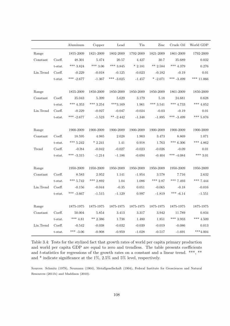
3.4 Test for Zero Production Growth Rates, Per Capita . . . . . . . . . . . . . . . 108
x
Introduction
This thesis consists of three independent chapters. Chapter 1 is joint work with Juliane Parys
and focusses on the allocation of parental leave between spouses. We modify a model of
collective rationality developed by Pierre-Andre Chiappori and coauthors (such as Browning
and Chiappori (1998)) to explicitly account for parental leave. The model predicts that the
ability of spouses to influence the allocation of parental leave depends on personal character-
istics such as age and income. Using representative data of households with young children
from Germany we show that a high relative age or income allows a spouse to reduce his or
her share in childcare. Chapter 2 is joint work with Mouhamdou Sy. We analyze the influ-
ence of increasing international trade on inflation. Increasing international trade makes firm
competition more fierce and leads to improving productivity through firm selection. All else
being equal, this reduces inflation. Chapter 3 is joint work with Martin Sturmer. In this
research project we link geological evidence to the historic developments of non-renewable
resource prices and its production in a model of endogenous growth to suggest that a range
of non-renewable resources could be considered inexhaustible. If the deterioration of resource
deposits in terms of ore grade and investments into extraction technology offset each other,
the total resource extraction cost per unit of the resource would stay constant. This could
explain the historic pattern of exponentially growing resource consumption at constant prices.
Even though the chapters are not related by content, they have a common approach. All
three chapters use an economic model to understand the underlying problem and test the
results empirically. Thus they contribute to the respective policy discussions by improving
the understanding of the problem and by empirically supporting the theoretical statements.
Chapter 1 is a topic from labor economics. It takes a microeconomic approach as it
analyzes the interaction of two individuals. It can have macroeconomic implications, however,
as it contributes to the understanding of why young parents stay in or leave the labor market,
1
with potentially large effects on the size and qualification of the labor force. Chapters 2 and
3 take macroeconomic approaches. Chapter 2 is a project in international economics and
chapter 3 combines growth and resource economics.
In the following the three chapters are described individually.
Chapter 1. The class of collective rationality models, which makes only minimal assump-
tions on the decision making process within the family and includes other decision-making
models like the axiomatic bargaining models. Since our research question does not necessitate
theoretical restrictions on the specific form of household decision-making, we use this model
class and adapt it to childcare allocation.
Small children must be in the custody of either one of the parents or of professional care
such as daycare centres or nannies. A parent can only work when he or she is not taking care
of the child. We consider the case of a country where the government pays parental benefits so
that no income loss results from childcare during the first year of the child. In this situation,
a parent does not need to be concerned about an immediate income loss. However, his or her
long-term income and career is affected, and as future income depends on the spouse’s own
human capital, long-term considerations will motivate the spouse to work as much as possible
and keep childcare low.
In a collective model spouses are assumed to have individual utility functions. This is
in contrast to unitary models and implies that there is a certain conflict of interest between
the spouses. The ability of an individual to influence the allocation of utility within the
household, sometimes termed the “bargaining power” of an individual, depends on individual
characteristics or “distribution factors”. Using survey data from Germany, we found that
those characteristics include relative income and age. Higher relative incomes and larger age
differences shift the conditional leave allocation towards the relatively poorer and younger
partner, respectively. In addition, we find that the share of professional childcare increases
with total household income.
The chapter has a potential policy relevance in that it contributes to the understanding of
the functioning of a government parental benefit scheme. It highlights the fact that long-term
career considerations play a role in the decision of childcare allocation and that a spouse’s
initial income may influence the couple’s decision even when there is no direct income loss
from interrupting the career.
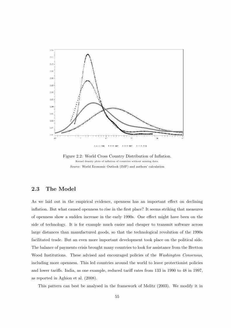
Chapter 2. This chapter is motivated by a remarkable empirical observation: In the
2
twenty years from 1990 to 2010, trade openness increased worldwide while inflation levels
decreased. Changes in inflation levels would normally be explained by changes in monetary
policy, and indeed, monetary policy changed much throughout this period. Rogoff (2003) lists
a number of substantial central bank measures which ended the Latin American hyperinfla-
tions at the beginning of the period under consideration and decreased inflation generally.
Taking a closer look at the figures, we searched for a more complete explanation of the
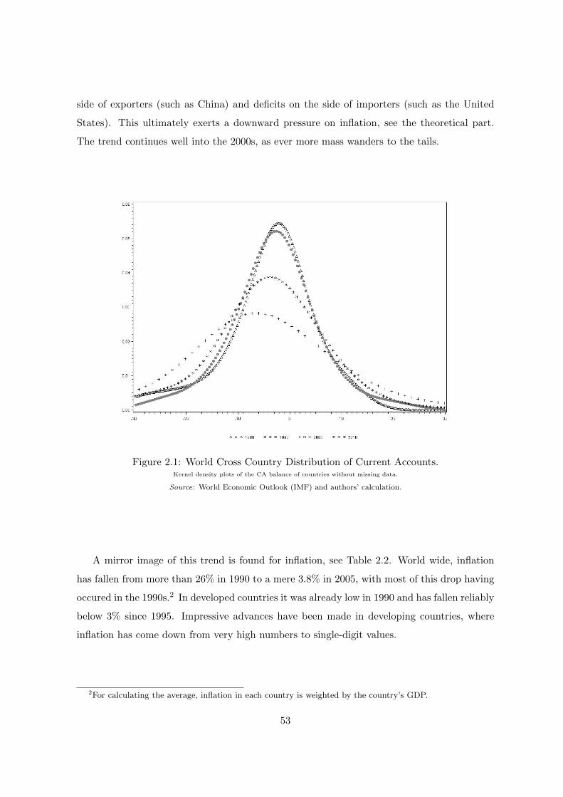
cause of the “Global Disinflation” as the phenomenon of decreasing inflation is referred to.
First, the trend cannot be explained by a dramatic change in a few economic “heavyweights”.
The entire distribution of openness and inflation across countries moved towards more open-
ness and lower inflation, respectively. As tables 2.1 and 2.2 show the development started
around 1990 and continued throughout the entire timespan without sudden jumps.
We build a model based on Melitz (2003) to analyze the link between disinflation and
globalization. Falling tariff rates reduce the effective transport costs faced by (potential)
exporters allowing them to ship a greater share of their production abroad. This increased
competition shifts a larger share of production towards more productive firms as very un-
productive firms leave the market and additional firms start exporting. Higher productivity
lowers the relative price of goods as the same amount of goods can be produced with less
labor input. A cash-in-advance constraint connects this change in relative prices to changes
in the price level: If the money supply does not systematically offset the effect of increasing
productivity, then inflation falls ceteribus paribus.
To verify the theoretical result empirically, we construct a new dataset of 123 countries
from various sources. As opposed to previous studies such as Chen et al. (2009) who find
this effect in regionally limited industry data, we are thus able to show the global scale of
the link between globalization and inflation. Controlling for openness and productivity, we
demonstrate the theoretical effect by interacting the two variables. The productivity variable
alone shows the effect of innovation activity while the interaction effect demonstrates which
contribution was made by the increased productivity caused by globalization.
This chapter highlights that globalization has an effect on inflation and that this effect is
temporary since it is the change in trade openness which accelerates the productivity increase.
The temporary nature of this particular effect of globalization may thus be of some relevance
to monetary policy.
Chapter 3. The last chapter is motivated by the apparent discrepancy between the
3
predictions of mainstream growth theory with respect to non-renewable resources and the
empirical evidence on the historic evolution of non-renewable resource prices and production.
Geological evidence shows that many important non-renewable resources are available in large
quantities in the earth’s crust. Deposits with ever decreasing resource density or “ore grade”
are exploited. Yet, growth models continue to work with the basic assumption of the model
by Hotelling (1931), where a fixed resource stock is exploited at an increasing price and
decreasing consumption of the resource. Historic evidence is at odds with this and shows
constant prices and increasing production and consumption in the long term.
These standard models can be found in standard textbooks on growth, take a very the-
oretical approach: Since the earth is finite, non-renewable resources are finite and thus the
global economy has to consume ever decreasing amounts of it if it wants to avoid the point
where nothing of the resource is left. Our claim is that this point of view is no useful de-
scription for historic patterns and the foreseeable future. The total amount of unexploited
resources is so immense that its current consumption rate could be maintained for centuries,
millennia or, in some cases, millions of years. This, however, does not imply that resources
can be used carelessly. The extraction comes along with large negative externalities, above
all for the environment. This aspect, however, is excluded from our research project as we
focus on the availability of the resource.
From the geological evidence we conclude that resources are available in principle, but at
different ore grades and difficulty of accessing them. This raises the question of extraction
costs. To analyze this question we consider two relationships. The first is the distribution of
a resource over ore grades. It answers the question of how many tonnes of a given resource
are available at a density of x percent of the resource per tonne of sediment. The second
relationship is between investments into extraction technology and ore grade that can be
profitably exploited. Our hypothesis is that these two relationships trade off such that the
cost of investment per tonne of the resource stays roughly constant over time.
Using this hypothesis in a model of economic growth, we are able to explain the historic
developments on resource consumption and prices: If the cost of the resource for extraction
and innovation in terms of capital stays constant over time, then a growing economy will
extract increasing amounts of it while the price remains stable.
This chapter may enrich our understanding of resource production and use by a combi-
nation of geological evidence and economic modelling. The supply of many resources may
4
not be the main concern for future economic growth. This insight should shift the focus even
more on the negative side effects of its use.
5
6
Chapter 1
Intra-Household Allocation of
Parental Leave
1.1 Introduction
Long labor market absence after the birth of a child causes a durable income and career
penalty due to forgone growth of human capital and a negative work commitment signal to
the employer for example.1 Traditionally, this has mainly been borne by mothers.2 However,
the allocation of childcare time, as far as it conflicts with market work, is increasingly subject
to change - especially in countries with a generous paid leave legislation. In this study,
we propose a model of how parents share parental leave and the income and consumption
drawbacks involved.
Treating a multiple-person household as a rational entity with a single set of goals has
been rejected by many economists.3 This is especially important for our study as it aims to
gain insight into the process that determines how parents share the time they spend on doing
childcare instead of working on the labor market. As an alternative to unitary household
models, Chiappori (1988, 1992) and Apps and Rees (1988) are the first to propose the most
1 Some of the early references are Mincer and Polachek (1974) as well as Corcoran and Duncan (1979). Theimportance of work experience for each spouse’s acquisition of human capital is formalized in chapter 6 of Ott(1992).
2 Ruhm (1998) reveals that brief parental leave periods (3 months) have little effect on women’s earnings,but lengthier leave (9 months or more) is associated with substantial and durable reductions in relative wageswithin Western European countries. Erosa et al. (2002) find that fertility decisions generate important long-lasting gender differences in employment and wages that account for almost all the U.S. gender wage gap thatis attributed to labor market experience.
3 A convincing empirical example is Lundberg et al. (1997).
7
general form of a collective model of household behavior. The key assumption is that, however
household decisions are made, the outcome is Pareto efficient. Browning and Chiappori
(1998), Chiappori et al. (2002) and Chiappori and Ekeland (2009) extend this model by
including distribution factors that affect household decisions even though they do not have an
impact on preferences or on budgets directly. The existence of distribution factors is crucial for
the model’s testability. Blundell et al. (2005) interpret the solution to the household problem
as a two-stage process, where household members share what is left for private consumption
after purchasing a public good.
The collective framework nests any axiomatic bargaining approach that takes efficiency
as an axiom. For instance, the Nash bargaining solution can be expressed as a maximization
of the product of individual surpluses. Each agent’s surplus involves the agent’s status quo
value which varies with personal characteristics and distribution factors. As pointed out in
Bourguignon et al. (2009), any efficient intra-household allocation can be constructed as a
bargaining solution for well-chosen status quo points.
There are very few theoretical examinations of the allocation mechanism between spouses
in the literature. One example is Amilon (2007), who analyzes temporary leave sharing in
Sweden using a Stackelberg bargaining model with a first-mover advantage for men due to
an unexplained “cultural factor”. In the empirical literature, the effect of different parental
benefit schemes across countries on parents’ childcare time contributions has been analyzed.
Ekberg et al. (2005), for example, evaluate the introduction of a “daddy month” in Sweden
and find an increase of fathers’ childcare time contribution, but no learning-by-doing effect
for childcare.
In this study, we introduce childcare sharing into a collective model of household behavior
with public consumption as in Blundell et al. (2005). Our model does not assume any innate
asymmetry between partners per se. It intends to explain the intra-household allocation of
childcare time and consumption while assuming Pareto optimality of the outcome. Couples
maximize a weighted household utility function. The Pareto weights have a clear interpre-
tation as “distribution of power” parameters. Bourguignon et al. (2009) provide testable
restrictions based on the presence of distribution factors which we exploit to empirically test
for collective rationality in parental leave sharing.
Parents can purchase professional childcare in order to reduce the total leave duration of
the household. This allows parents to work and thus invest in their human capital, which
8
increases consumption of both partners in the future. In this sense, it can be thought of as
a “public good”. The household decision process can be imagined to happen in two stages.
Parents first agree on how much professional childcare to purchase, and then, conditional on
the level of public good consumption and the budget constraint stemming from stage one,
determine their individual levels of private consumption and labor market participation at
the second stage. The model predicts that households with higher incomes purchase more
professional childcare.
Our model predicts that once the level of public consumption is set, the weaker spouse
takes more leave time than the partner with more power. The more one contributes to
household income and the older a partner is relative to the spouse, the larger is his or her
intra-household power translating into less parental leave and a larger consumption share.
Although income during leave is mainly replaced through parental benefit, both parents value
labor market work as an input to human capital positively impacting their relative income
and therefore their private consumption shares later in life.
If we consider for example an increase in the income of one partner, this strengthens that
partner’s power in the household and allows him or her to shift some leave time to the spouse.
The net effect on the spouse’s leave duration is not straightforward. On the one hand, there
is a wealth effect stemming from the household income increase, which allows the couple to
purchase more professional childcare. On the other hand, the change in Pareto weights leads
to a redistribution of leave time between parents.
Generous parental leave benefits as introduced in many European countries keep household
income stable after the birth of a child, no matter who stops working in the market in favor
of childcare. Parents are therefore motivated to work mainly out of concern for their human
capital. This determines their future income and also their power to influence decisions. This
endogenization of gender power has been theoretically explored by Basu (2006), Iyigun and
Walsh (2007a) and Iyigun and Walsh (2007b). We apply these theoretical concepts in a basic
form.
Our model’s empirical restrictions are tested using survey data on young German families.
The German legislation allows both parents to go on paid leave and receive generous benefits
replacing 67-100 percent of the average monthly net income from before the child’s birth. The
law allows leave time allocation between parents to be relatively flexible. We cannot reject
Pareto efficiency in leave sharing. The data also confirm the income effects predicted by the
9
collective model.
The chapter is organized as follows. Section 1.2 introduces a collective model of intra-
household childcare and consumption sharing. An overview of the legal parental benefit
situation in Germany in 2007 and a data description are provided in Section 1.3. In Section
1.4, we empirically test our collective model and its predictions. The last section concludes.
1.2 A Collective Model of Parental Leave Sharing
1.2.1 Unitary, Non-cooperative and Collective Household Models
For decades, most theoretical and applied microeconomic work involving household
decision-making behavior has assumed that a household behaves as if it had a single set of
goals. Following Browning and Chiappori (1998) we refer to them as unitary models. In the
unitary household model, the partners’ utility functions represent the same preferences such
that their joint utility is maximized under a budget constraint. More precisely, a weighted
sum of utilities is maximized, but the weights are fixed. This does not take into consideration
that spouses might have conflicting interests and that the degree to which they can influence
household decisions might depend on individual characteristics.
Factors that enter neither individual preferences nor the overall household budget con-
straint but do influence the decision process are known as distribution factors. A model with
a weighted sum of individual utility functions is formally a unitary model as long as the
weights do not depend on these distribution factors.
In order to study the intra-household decision process on parental leave allocation we apply
a collective setting as in Blundell et al. (2005) to explicitly model the conflict of interests
between partners. Let us consider an increase in income for the woman to illustrate how
the two models react differently. The additional income increases the household income.
Through this wealth effect the couple can afford more, including professional childcare. In
the unitary model, both partners share this gain equally, so that both would do less childcare.
The collective model considers a bargaining effect in addition. The woman increases her
bargaining weight, so she gets a greater share of the increased wealth. Both effects are to
her advantage. The man, however, benefits from the increased wealth, but suffers from a loss
in bargaining power. The net effect of the woman’s increase in earnings may be positive or
negative for him, depending on specific functional forms. Thus only the collective model is
10
able to explain a decrease in childcare of one partner as a result of an increase in income for
the other partner.
But even if we accept a certain conflict of interest and bargaining weights that depend
on distribution factors, the class of models to be chosen is not obvious. Non-cooperative
models do not assume efficiency as the collective model does and instead assume that each
household member maximizes his or her own utility without regard for the utility of the spouse.
This potential way of resolving conflict in the household has been advanced by Konrad and
Lommerud (1995), for example. But unlike the collective model, this theoretical concept
hasn’t been shown empirically. It is not motivated as a general concept, but for specific
uses such as threat points in a cooperative model as suggested by the authors. Another
application is illustrated in the “semi-cooperative” model of Konrad and Lommerud (2000)
where there is a non-cooperative period before the family is formed and a cooperative period
after it is formed. We therefore follow Konrad and Lommerud (2000) when they say “Fully
non-cooperative behavior, we hope, is rare in family contexts...”, and model family decision-
making after the birth of a child as cooperative.
1.2.2 Model Setup
Resources to be allocated in the household are time and money, whereby the latter is
translated into consumption. Time allocation has a central role in our model of household
behavior. It concerns working time during the period right after the birth of a child, called
period 1. During working hours there are only two possible activities for parents: market work
and childcare. A parent not being on leave is free for market work. Therefore, shortening leave
time is equivalent to extending work time.4 Work experience is valued as an input to human
capital accumulation. It increases income and consequently the individual consumption share
in the second period. In addition, a long leave period might imply career drawbacks as it
signals weak work commitment to the employer and promotion rounds might be missed.
Our model focusses on two main trade-offs involved with the intra-household allocation of
parental leave: One trade-off concerns the consumption allocation between partners. Child-
care provided by a parent him- or herself reduces that parent’s market working time. Al-
though income is replaced to a large extent through parental benefit during the leave period
itself, parenthood-related job absence still involves an income penalty after returning to work
4 The basic form of the model does not include any explicit measure of leisure, because we focus on theextensive margin of labor supply. See section 1.2.4 for a model including leisure.
11
compared to a situation without any career interruption.
The second major trade-off is between consumption during the period right after birth,
when the child is very young and needs intensive care, and later. Parents can hire profes-
sional childcare such as nannies, daycare facilities, etc, in order to reduce the total household
parental leave time.5 The more professional childcare parents purchase, the more it reduces
the household’s level of private consumption in period 1, but the more it also allows part-
ners to reduce parenthood-related income and consumption drawbacks for the second period.
The amount of public expenditures therefore determines the total amount of leave time the
household needs to take. Given the central role of time use we begin by defining its allocation.
Time Constraints
In period 1, which are the T1 months after delivery, each parent i has to allocate time
between market work hi and leave bi:
T1 = hi + bi, i ∈ {m,w} . (1.1)
Men are indexed i = m and women i = w. Permanent childcare needs to be guaranteed ei-
ther by parents providing childcare themselves, denoted bm and bw, or by hiring professional
childcare, denoted bp, such that
T1 = bm + bw + bp . (1.2)
This equation ensures that someone takes care of the newborn at any time. Market work
and childcare time are restricted by zero below and by T1 above. For future reference, note
that a woman can work on the labor market whenever she is not on leave, i.e. hw = T1 − bw,
and that a man’s work time can be expressed as the time when either the woman is at home
or professional childcare is hired, i.e. hm = bw + bp.
Income and Budget Constraint
Monthly net income is denoted wit, where i ∈ {m,w} denotes the spouse concerned and
t ∈ {1, 2} is the time period. Total net income of partner i in period t is consequently given
by witTt. In the first period, parents have two ways of spending income: They can either
consume private goods, or purchase professional childcare at a monthly rate wp. The latter is
5 Modeling different childcare qualities is interesting, but not the focus of the current model. Therefore, weassume all three sources of childcare to be perfect substitutes.
12
considered a public good that shortens the cumulative leave duration of both partners. The
level of public good consumption is denoted bp. The couple’s budget constraint is thus
cm1 + cw1 + bpwp = (wm1 + ww1) T1 . (1.3)
The right-hand side of the above equation implies that parental benefit is assumed to
compensate for the most part of the immediate income loss parents encounter from going
on leave. Consequently, our model focusses on the long-term drawbacks from parenthood-
related job absence. It applies especially to countries with generous paid leave regulations.
However, direct income reductions during leave could be easily incorporated through multi-
plying monthly net income of the parent on leave by an income-reduction factor λ, where
0 ≤ λ < 1. λ = 0 reflects the situation of countries with unpaid parental leave, whereas our
model assumes full income replacement, i.e. λ = 1.
Utility and Human Capital
Parents derive utility from consumption and from the well-being of their child. The utility
derived from having a kid and its well-being explains a couples’ demand for children. How-
ever, once the decision for a child has been made, the derived utility is constant6 given that
at least one appropriate person takes care of it. Thus, we model consumption in each of the
two periods as the variable to be maximized. The utility function is given as
Ui = U(ci1, ci2) (1.4)
with the standard properties of positive but diminishing returns to consumption in both
periods.
Our model incorporates public and private consumption. As in Blundell et al. (2005),
partners share what is left for private consumption after purchasing a public good. We argue
that relative incomes and the age difference between partners strongly influence the intra-
household distribution of power and therefore determine the individual private consumption
shares. The higher a partner’s relative income or the older a partner is compared to the
spouse, the more private goods he or she can consume.
The level of public consumption implicitly determines the amount of time parents can
work on the market in order to accumulate human capital and raise future earnings. Since
utility from the child’s wellbeing is constant, professional childcare impacts utility only in-
6 See Chiappori and Weiss (2007) for an example of this assumption in the literature.
13
directly via the budget constraint. For the allocation of consumption, we focus on private
consumption for two reasons: First, private consumption is especially important to both part-
ners as it remains to a large extend even after a potential marital dissolution. Second, we
want to investigate the impact of the intra-household distribution of power on consumption
shares, and public consumption is not affected by changes in the power allocation.
Pareto Weights
Partners maximize a weighted sum of utilities. The resulting allocation of household
resources is assumed to be Pareto optimal. The man’s Pareto weight is denoted by µ(z) ∈
[0, 1], that of the woman by 1 − µ(z).7 The weights reflect the power of each partner and
depend on a Q-dimensional vector of distribution factors z. Examples for observable and
unobservable distribution factors from the literature include relative incomes, age difference,
relative physical attractiveness, and the local sex ratio. In the context of childcare, custody
allocation and alimony transfers from the custody to the non-custody parent after divorce are
further examples.
Assuming that µ(z) is known to be increasing in z1, which could be the man’s relative in-
come or relative physical attractiveness for example, and decreasing in z2, the negative age dif-
ference between partners [-(male minus female age)] for example, we can write ∂µ(z)/∂z1 > 0
and ∂µ(z)/∂z2 < 0. The man’s relative income wm1/ww1 as a distribution factor implies c.p.
the Pareto weight µ(z) to be increasing in the man’s monthly contribution to total household
income wm1 and to be decreasing in the woman’s contribution ww1, i.e. ∂µ(z)/∂wm1 > 0 and
∂µ(z)/∂ww1 < 0.
First-Period consumption
We allow parents to hire professional childcare during working hours in period 1. This
lowers the current level of private consumption, but shortens the period of parenthood-related
labor market absence in period 1 thus increasing the level of private consumption in period
2. Therefore, the level of expenditures on professional childcare in period 1 is equivalent to
an intertemporal consumption allocation within the household.
7 If µ(z) = 1 the household behaves as though the man always gets his way, whereas if µ(z) = 0 it is asthough the woman were the effective dictator. For intermediate values, the household behaves as though eachperson has some decision power.
14
Second-Period consumption
First-period monthly net income wi1 reflects the level of human capital from schooling and
work experience acquired up to the child’s birth. The income level in period 2 depends on
first-period income wi1, on the labor market experience from period 1, hi, and on the initial
level of human capital from before period 1, hi0. For all i ∈ {m,w}, we write
wi2 = (hi + hi0)wi1 . (1.5)
Second-period household income (ww2 + wm2)T2 is allocated between partners and spent
individually on private consumption. The allocation underlies the same collective decision-
making process as in the first period. Any change in the distribution of parental leave has,
via second-period income, a WE as well as a BE in the second period. The motivation of
spouses to reduce own leave time comes from the intention to (i) increase own future income,
(ii) c.p. increase relative income, i.e. strengthening the own bargaining weight in period 2,
and (iii) ultimately increase own future consumption. Labor market work in the first period
is thus an investment into the future bargaining weight. See 1.A.1 for an analytical solution
of the collective decision in period 2.
Dynamic household bargaining models are complex to solve analytically. Modeling a bar-
gaining process in both periods renders the model dynamic. Mazzocco (2004) and Mazzocco
(2005) model two periods, but the bargaining weight of the spouses is assumed to be fixed
over time. In Mazzocco (2007) the weights are only influenced by random exogenous shocks.
Basu (2006), Iyigun and Walsh (2007a) and Iyigun and Walsh (2007b) do have endogenous
bargaining weights. The complexity of the models however allows only for quite general
results.
In order to obtain analytical solutions, which we can test empirically, we take a shortcut
and model consumption in period 2 directly as a function increasing in work experience and
If we assume that only relative income matters for the leave time sharing rule, then we can
check the proportionality condition by testing whether the sum of the log income coefficients
equals zero, i.e. whether
βi1 + βi2 = 0 ∀ i ∈ {m,w} .
This hypothesis cannot be rejected - neither individually nor jointly across models. Therefore,
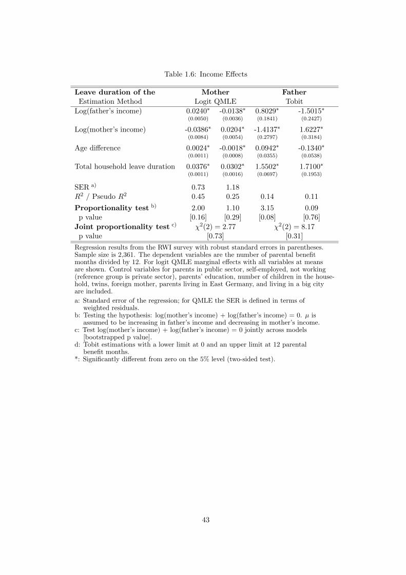
Table 1.6 provides further pieces of evidence for Pareto optimality in parental leave sharing
as the Wald tests can again not reject the proportionality hypothesis.
In addition, we present estimates of Tobit models with a lower censoring at 0 and an
upper censoring at 12 months of paid leave. The magnitudes of the income effects are larger
in absolute terms than in the fractional logit regressions as the Tobit models focus on interior
solutions.12 Families who do not opt for a corner solution, i.e. where each partner takes
a strictly positive leave time, are likely to react stronger to a change in relative incomes as
compared to partners opting for a corner solution. This is because the decision to temporarily
drop out of the labor market has been already taken by both parents.
Robustness Check 2: z-Conditional Demands
Further testable implications come from an alternative demand system that is consistent
with collective rationality. It follows from the effect of distribution factors on the intra-
household allocation being one-dimensional, which is implied by the proportionality condi-
tion. Independent of the number of distribution factors, they can influence the parental leave
allocation among parents only through a single, real-valued function µ(z). The demand for
one good can therefore be expressed as a function of the demand for another good.
Bourguignon et al. (2009) introduce z-conditional demands which are useful to resolve, e.g.,
the empirical difficulty of nonlinear Wald test statistics being noninvariant to reformulations
of the null hypothesis. We follow Bobonis (2009) and construct linear Wald tests based on
parametric versions of the z-conditional demand functions in order to assess the robustness
of our previous results to reformulations of the null hypotheses.
The idea of z-conditional demands is demonstrated in the following for G(·) being the
logistic function. Under the assumption that relative income wm1n/ww1n has a strictly mono-
12 Note that the dependent variables in columns 2 and 4 of Table 1.6 are not rescaled. Therefore, coefficientsdo not need to be multiplied by 12 as in the other tables.
28
tone influence on optimal leave sharing, we can invert (1.20):
wm1n
ww1n=
1
αi1log
(hin
1− hin
)− αi0αi1− αi2αi1
agediffn −αi3αi1
btotn
− 1
αi1fi(an)− 1
αi1εin ∀ i ∈ {m,w} .
As total household leave duration is simply the sum of maternity and paternity leave time,
we can replace btot by bin + 12hjn. For parent j with j ∈ {m,w} and j 6= i, we can substitute
the above equation into (1.20) to obtain13
E[hjn|xn] = G
(1
αi1(1− 12αj3) + 12αi3αj1
[ (αi1αj0 − αi0αj1
)+(αi1αj2 − αi2αj1
)agediffn
+(αi1αj3 − αi3αj1
)bin + αj1 log
(hin
1− hin
)+(αi1 fj(an)− αj1 fi(an)
)]
).
Benchmark OLS and fractional logit regression results are provided in Table 1.7. As ex-
pected we find that the mother’s contribution to total household income has no significant
impact on either maternity or paternity leave duration anymore once we control for the part-
ner’s leave duration. This must be true if the collective model is correct as the father’s con-
tribution to household income as one distribution factor already absorbs the one-dimensional
effect of all distribution factors together on parental leave sharing.
Robustness Check 3: First Births and Tobit Estimations
A concern might be that in families, who already had children before the most recent one,
parents might have specialized in different activities. Mothers might have provided the larger
share of childcare already for the older children and are therefore relatively more productive
in childcare provision than fathers. In this sense the lower market income of women reflects
their specialization in household production and not their lower intra-household power.
In order to address this concern we restrict our sample to families without any older chil-
dren, which reduces the sample to about 57 percent of the full sample. We redo the fractional
13 Note that, if G(·) is linear, total household leave duration becomes redundant once we control for thepartner’s leave duration and
logit estimations of Table 1.5 and find a similar picture as before. As in Table 1.6 we compare
the estimates of our previous analysis with the results of Tobit model estimations and can
completely confirm our findings from before.
Concerns and Limitations
The variation in relative income and age difference between households could be correlated
with unobservable characteristics of couples like varying separation probabilities. In this case
couples with a lower risk of divorce may have different preferences for childcare sharing than
partners with a high risk of separation. The considered distribution factors would then have
an indirect effect on the sharing rule through the effect on divorce probabilities. However,
Bobonis (2009) points out that tests of the proportionality condition are not invalidated
by this possibility since the ratio of the direct and indirect effects of changes in relative
income and/or age difference on Pareto weights does not involve anything specific to either
maternity or paternity leave durations. Effects of changes in those factors on leave durations
are again equally proportional to the distribution factors’ influence on the intra-household
power distribution.
Another concern addresses unobserved heterogeneity in distribution factor effects on in-
dividual leave durations, which involves the possibility of differences in estimated coefficients
stemming from heterogeneity in individuals’ preferences rather than from differences in indi-
viduals’ intra-household power. Changes in the age difference might for example affect total
household leave durations mainly in the lower range of the distribution between 0 and 12
months if age difference mainly affects maternity leave duration in a way that in couples with
a small age difference women rather take paid leave for less than the maximum duration.
Men’s relative income, on the other hand, might affect more the upper range of the leave
distribution between 12 and 14 months because relatively better earning men, i.e. relative to
their spouses, mainly decide whether to participate in parental leave at all and are unlikely
to take more than the minimum requirement of two months.
The main consequence would be that Pareto optimality tests, which rely on testing con-
dition (1.21), may consider significant differences between the ratios of distribution factor
coefficients in the demand for different goods as evidence against the predictions of the col-
lective model. In fact, however, rejections of the proportionality condition could be caused
by heterogeneity in household demand functions. As we cannot reject Pareto efficiency in
parental leave sharing, this concern does not seem to be harmful in our application.
30
Finally, if individuals’ preferences for leisure are not separable from those for leave time
or childcare, respectively, the estimated income effects may suffer from an omitted variable
bias. We therefore assume that conditioning on employment status before birth, employment
sector, and additional socioeconomic and demographic variables, preferences for leisure are
separable from those for childcare. A related limitation of relative income as a distribution
factor is that labor incomes may be endogenous to households’ childcare allocation decisions.
Due to a lack of observed non-labor income or exogenous variation in incomes, we need to
focus on correlations of relative incomes with household demands.
1.4.3 Empirical Intra-Household Allocation of Parental Leave
Concerning Proposition 1.1
Proposition 1.1 addresses the importance of distribution factors that do not enter indi-
vidual preferences, but influence the decision process. The presence of such variables is not
consistent with the unitary framework. Examples of distribution factors in the absence of
price variation that have been suggested in the literature, include relative incomes, age dif-
ference, relative physical attractiveness, and local sex ratio. In the context of leave sharing,
custody allocation after divorce and alimony transfers from the custody to the non-custody
parent are also examples of distribution factors. Due to a lack of substantial variation in the
other potential distribution factors between the 16 German states,14 for the empirical analysis
we need to focus on relative income and age difference changes while controlling for the level
of household income. A unitary model would predict that only the level and not the sources
of household income matter.
Table 1.5 provides evidence for collective rationality in parental leave sharing by confirm-
ing the impact of relative income changes on individual leave durations. A higher relative
income of the father and a larger age difference are correlated with longer maternity leave
and shorter paternity leave. Once we include relative income, the level of household income
does not have a significant impact on parental leave durations anymore. This finding provides
evidence for the WE on paid leave durations being weaker than the BE.
Concerning Proposition 1.2
Proposition 1.2 predicts that each spouse’s leave share is decreasing in own income. Em-
14 Unfortunately, we do not observe smaller geographical regions than states.
31
pirical support for this prediction is presented in Table 1.6.15 The magnitudes of the Tobit
parameter estimates from Table 1.8 tell us that doubling the mother’s income leads to a 1.4
months decrease of her own parental benefit duration. For fathers the corresponding coeffi-
cient from the last column of Table 1.6 is a little bit larger in absolute terms: it corresponds
to a month and a half decrease.
Additionally, doubling the mother’s earnings involves an increase in the father’s leave time
of about four fifth of a month. If the father’s income is doubled, the coefficient is more than
twice as big, i.e. mothers go on leave for 1.6 months longer. The magnitude of the coefficients
might even be expected to become larger in absolute terms in the future if we consider that
the most recent data available are from the first third of 2007 - the four months after the new
parental benefit legislation has been introduced in Germany.
Tables 1.1 and 1.2 demonstrate a strong asymmetry between maternity and paternity
leave durations on an aggregate level. Table 1.1 tells us that, based on the Parental Benefit
Statistic, for 95.3 percent of the children born in 2007 the mother went on leave for at least
one month. This number needs to be compared to only 13.3 percent of fathers who took at
least one month off. Table 1.2 then shows that fathers take only 5.3 percent of the total leave
duration.
However, if we look at the development of fathers’ participation rate in parental leave
in Scandinavian countries, who introduced generous parental leave legislations much earlier,
paternity leave durations in Germany can be expected to increase in the future.
Concerning Proposition 1.3
Proposition 1.3 predicts that professional childcare use increases with household income,
but is independent of distribution factors. The consumption of the public good determines
the amount of household leave time which is then shared between parents.
Some descriptive facts from RWI survey data are that 30.7 percent of parents with a
monthly household net income below EUR 2,000 plan to hire professional childcare. This
percentage rises with income until it reaches 55.4 percent for parents with a household in-
come of more than EUR 5,000. Marginal effects from logit QMLE in Table 1.9 suggest that
only household income and not relative income or age difference matter for the decision to
hire professional childcare. In particular, a family is roughly 2.4 percent more likely to hire
professional childcare if monthly household net income exceeds the average income of house-
15 See also Tables 1.5 and 1.8.
32
holds by EUR 1,000.16
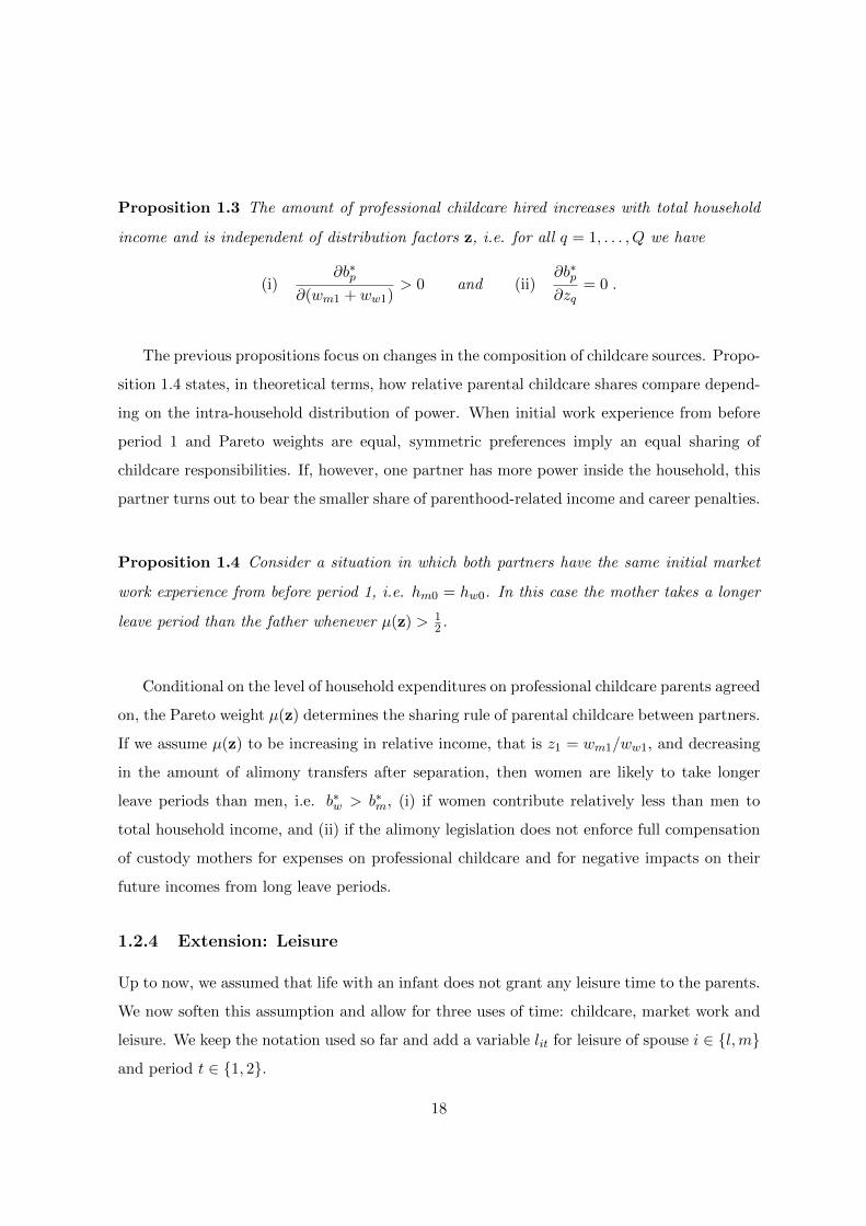
Concerning Proposition 1.4
Proposition 1.4 states that the mother’s leave share is relatively larger if the father’s
Pareto weight is relatively stronger. This theoretical result is difficult to bring to the data,
as the exact functional form of the power function is unknown. A multiplicity of factors are
likely to determine the exact intra-household “distribution of power” out of which we observe
substantial variation only in two distribution factors (relative income and age difference).
We still provide suggestive empirical evidence for women to be represented in childcare
relatively stronger than their partner in couples where the woman’s Pareto weight is relatively
weaker, i.e. when 1 − µ(z) < µ(z). We construct a dummy variable which equals one if the
woman takes more leave time than the man. A second dummy equals one if the man’s
contribution to household income is bigger than the woman’s. Then, families in which the
latter dummy variable equals one are 5.1 percent more likely that the woman takes relatively
more leave time than families where the man’s relative income is less than 1.17
However, while in 65 percent of the observed households from the RWI survey the man’s
relative income is larger than 1 and in 73 percent the man is older that the woman, in more
than 89 percent of households the woman’s relative leave time is larger than 1. This means
that, as the effect of all distribution factors on the intra-household allocation of leave time is
one-dimensional, we are able to infer the effect of changes in the observed distribution factors
on relative leave times to happen through changes in relative Pareto weights. Still, we cannot
credibly predict the exact magnitude of the man’s and the woman’s Pareto weight in a given
household without knowing the exact functional form and without observing all arguments
of the power function.
1.5 Conclusion
This chapter aims to gain insight into the process that determines how parents share the
time they spend on doing childcare instead of working on the labor market. Lengthy parental
leave periods involve long-term income and career penalties even in countries with a generous
16 As the dependent variable is a dummy, logit QMLE simplifies to a usual logit estimation. We calculatemarginal effects with all variables at means. Qualitative results for different covariate values are similar andavailable from the authors upon request.
17 The t statistic of the marginal effect is 4.2 when regressing the leave-time dummy on the relative-incomedummy in a logit regression while using the same remaining controls as in Table 1.5.
33
paid leave legislation. Therefore, both parents value labor market work as an input to their
human capital that positively impacts their individual incomes later in life - which translates
into a higher level of future private consumption.
We introduce parental leave sharing in a collective model of household behavior with
public consumption. The model’s restrictions are tested on survey data of young German
families. The collective model is identified through the existence of distribution factors that
affect household decisions even though they do not impact preferences nor budgets directly.
Although all decisions happen simultaneously, the leave allocation can be imagined to
happen in a two-stage process: Parents first agree on public expenditures on professional
childcare use. Then, and conditional on the amount of public good consumption, partners
choose the time they spend on childcare and their levels of private consumption. Each part-
ner’s leave time is the shorter and private consumption is the higher, the stronger a partner’s
power initially is. Market work is valued as an investment in human capital which increases
expected future income. A higher personal income c.p. increases the household income and
the relative income. It therefore translates into a higher consumption level for the household
and a larger personal consumption share through a stronger Pareto weight. Households face
one trade-off concerning the allocation of childcare time conflicting with work time between
partners, and a second trade-off related to an intertemporal private consumption allocation
between the nearer and the farther future by choosing the amount of professional childcare
to hire.
To summarize, parental leave time and the involved income and career penalties are allo-
cated strongly towards women. This is correlated to men usually contributing relatively more
to household income and being older than their partner. Possibly, the economically weak out-
side option for women as a single mother even boosts the inequality in leave time sharing.18
Still, as we observe in the data, the childcare allocation is sensitive to relative incomes and
age differences. It is more equal in households where the woman contributes relatively more
to household income and where the woman is relatively older.
18 Alimony transfers by the father help to reduce the inequality after divorce, but DiPrete and McManus(2000) and Bartfeld (2000) among others find that the economic situation of custodial-mother families is stilldramatically worse than the economic situation of fathers after separation.
34
Appendix to Chapter 1
1.A Mathematical Appendix
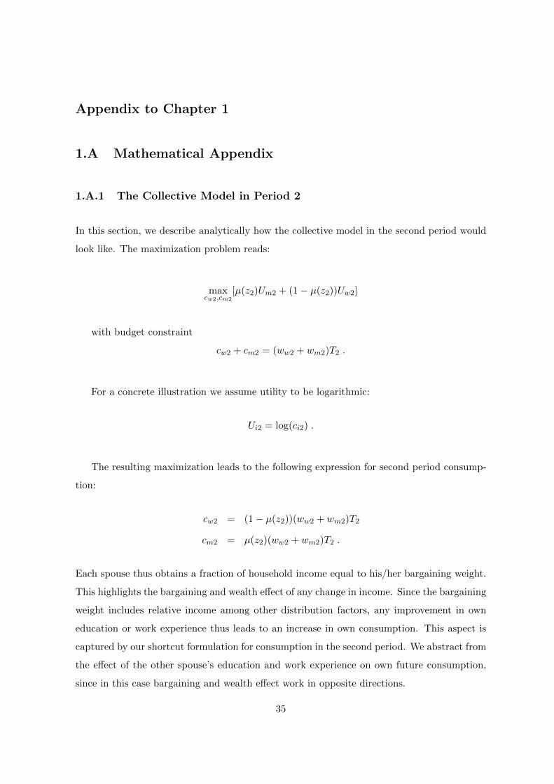
1.A.1 The Collective Model in Period 2
In this section, we describe analytically how the collective model in the second period would
look like. The maximization problem reads:
maxcw2,cm2
[µ(z2)Um2 + (1− µ(z2))Uw2]
with budget constraint
cw2 + cm2 = (ww2 + wm2)T2 .
For a concrete illustration we assume utility to be logarithmic:
Ui2 = log(ci2) .
The resulting maximization leads to the following expression for second period consump-
tion:
cw2 = (1− µ(z2))(ww2 + wm2)T2
cm2 = µ(z2)(ww2 + wm2)T2 .
Each spouse thus obtains a fraction of household income equal to his/her bargaining weight.
This highlights the bargaining and wealth effect of any change in income. Since the bargaining
weight includes relative income among other distribution factors, any improvement in own
education or work experience thus leads to an increase in own consumption. This aspect is
captured by our shortcut formulation for consumption in the second period. We abstract from
the effect of the other spouse’s education and work experience on own future consumption,
since in this case bargaining and wealth effect work in opposite directions.
35
1.A.2 FOC, SOC, Non-negativity Constraints and Proofs
First- and Second-Order Conditions
Assuming for the moment that the non-negativity constraints are nonbinding,19
the FOCs are
L(1,0,0) =µ(·)
bw + bp + hm0− 1− µ(·)T1 − bw + hw0
≡ 0
L(0,1,0) = − µ(·)(wm1 + wm1)T1 − wpbp − cw1
+1− µ(·)cw1
≡ 0
L(0,0,1) = µ(·)(
1
bw + bp + hm0− wp
(wm1 + wm1)T1 − wpbp − cw1
)≡ 0
This is a linear equation system in three variables. Results are given in Section 1.2.2.
The Hessian of L is given by
H =
L(2,0,0) L(1,1,0) L(1,0,1)
L(1,1,0) L(0,2,0) L(0,1,1)
L(1,0,1) L(0,1,1) L(0,0,2)
with
L(2,0,0)(b∗w, c∗w1, b
∗p) = − µ
(b∗w + b∗p + hm0)2− 1− µ
(T1 − b∗w + hw0)2< 0
L(0,2,0)(b∗w, c∗w1, b
∗p) = − µ
((wm1 + ww1)T1 − wpb∗p − c∗w1)2− 1− µ
(c∗w1)2< 0
L(0,0,2)(b∗w, c∗w1, b
∗p) = −µ
(1
(+b∗w + b∗p + hm0)2+
w2p
((wm1 + ww1)T1 − wpb∗p − c∗w1)2
)< 0
L(1,1,0)(b∗w, c∗w1, b
∗p) = 0
L(1,0,1)(b∗w, c∗w1, b
∗p) = − µ
(b∗w + b∗p + hm0)2< 0
L(0,1,1)(b∗w, c∗w1, b
∗p) = − µ wp
((wm1 + ww1)T1 − wpb∗p − c∗w1)2< 0
The first minor is negative, the second is |H2| = L(2,0,0)L(0,2,0) > 0. The determinant of the
Hessian at the maximum is
19 See next section for details on the non-negativity constraints.
36
|H3(b∗w, c∗w1, b
∗p)| = L(2,0,0)(b∗w, c
∗w1, b
∗p) L(0,2,0)(b∗w, c
∗w1, b
∗p) L(0,0,2)(b∗w, c
∗w1, b
∗p)
−L(2,0,0)(L(0,1,1)(b∗w, c
∗w1, b
∗p))2− L(0,0,2)(b∗w, c
∗w1, b
∗p)(L(1,0,1)(b∗w, c
∗w1, b
∗p))2
< 0 .
Therefore, the Hessian is negative definite at (b∗w, c∗w1, b
∗p) and L(b∗w, c
∗w1, b
∗p) is a maximum.
The Non-negativity Constraints
When solving the maximization problem (1.8), we consider only the case where the non-
negativity constraints are nonbinding. We then use the resulting solutions to derive our
propositions. In order for this to be meaningful, we have to show that there exists a range of
parameters, for which the non-negativity constraints are indeed nonbinding.
From equation (1.9) and (1.12) it can be seen that if the Pareto weight of one spouse equals
zero, this leads to an excessive leave duration for the other spouse, i.e. µ(·) = 0 ⇒ b∗m ≥ T1
and µ(·) = 1 ⇒ b∗w ≥ T1. The interpretation is that if the utility of one spouse has no
importance, then this partner would be overly exploited in favor of the other. The non-
negativity constraints therefore only hold for an intermediate range of weights µmin(·) to
µmax(·) with 0 < µmin(·) < µmax(·) < 1. Outside of this range, a corner solution with bm = 0
or bw = 0 maximizes the household’s utility. In the following, we show that all constraints
can hold at the same time, so that we are not in a degenerate case.
The non-negativity constraints for the duration of maternity and paternity leave can be
written:
b∗w ≥ 0
⇔ (1 + µ(·)) T1 + hw0
2− (1− µ(·)) (wm1 + ww1)T1 + wphm0
2wp≥ 0
⇔ (wm1 + ww1)T1 − wpT1 + wp(hm0 − hw0)
(wm1 + ww1)T1 + wpT1 + wp(hm0 + hw0)≤ µ(·) and
b∗m ≥ 0
⇔ (2− µ(·))T1 + hm0
2− µ(·) (wm1 + ww1)T1 + wphw0
2wp≥ 0
⇔ 2wp(T1 + hm0)
(wm1 + ww1)T1 + wpT1 + wp(hm0 + hw0)≥ µ(·)
37
The non-negativity constraints for b∗m and b∗m can be simultaneously fulfilled only if
The partial derivatives of L′ with respect to the seven endogenous variables is a linear
equation system with the solution indicated in the proposition statement. 2
39
1.B Tables
Table 1.1: Composition of Households that Use Parental Benefit
Case Frequency FractionOnly the mother made use of the parental benefit 362,368 86.7%Only the father made use of the parental benefit 19,526 4.7%Both mother and father made use of the parental benefit 35,938 8.6%
Total 417,832 100.0%
Source: Authors’ calculations from the Parental Benefit Statistic 2007.
Table 1.2: Duration of Parental Benefit Use by Gender
Women MenDuration in months Frequency Fraction Frequency Fraction
Source: Authors’ calculations from the RWI survey. Only leave takers(benefit duration ≥1 month).
40
Table 1.4: Summary Statistics
RWI Survey of Children Born in January till April 2007
Variable Description Mean Std.Dev. Obs.Number of benefit months: Mother parental benefit duration in 10.15 3.45 4,177Number of benefit months: Father months (range: 0-12) 1.03 2.63 4,177Household benefit duration (range: 0-14) 11.18 2.98 4,177
No benefit use: Mother dummy (d) =1 if the num- 0.08 0.27 4,177No benefit use: Father ber of benefit months = 0 0.76 0.43 4,177
Professional childcare d=1 if used 0.36 0.48 4,151
Mother’s income (range: 0.08-6.0) 0.98 0.81 3,536Father’s income (range: 0-6.0) 1.72 1.11 3,228Household income (range: 0.3-12) 2.78 1.44 3,130
Net monthly income in tEUR, means from categories= EUR 225 for below EUR 300 income category; = EUR 6,000 for above EUR 5,000 category
Age difference (range: -25 - +35) 3.00 4.85 4,131(Father’s) Relative income (range: 0-59) 3.10 3.85 3,130
Mother in public sector d=1 if working in 0.06 0.25 4,017Father in public sector public sector 0.07 0.24 3,523Mother in private sector d=1 if working in 0.53 0.50 4,017Father in private sector private sector 0.71 0.45 3,523Mother is self-employed d=1 if self-employed 0.04 0.20 4,017Father is self-employed 0.11 0.31 3,523
Mother secondary school d=1 if highest education 0.46 0.50 4,177Father secondary school level is secondary school 0.47 0.50 4,177Mother high school d=1 if highest education 0.24 0.43 4,177Father high school level is high school 0.18 0.39 4,177Mother college/university d=1 if highest education 0.26 0.44 4,177Father college/university level is college/university 0.28 0.45 4,177
Age of the oldest child (range: 0-24) 2.44 3.83 4,149Children number (range: 1-11) 1.75 0.95 4,177Twins d=1 if multiple births 0.02 0.14 4,177
Mother is foreign d=1 if not German 0.11 0.31 4,142East d=1 if living in the East 0.09 0.28 4,078Big city d=1 if ≥ 100T inhabitants 0.27 0.45 3,868
Parental Benefit Statistic 2007 (Couples)Number of benefit months: Mother parental benefit duration in 11.15 3.09 35,938Number of benefit months: Father months (range: 1-12) 2.69 2.05 35,938Household leave duration (range: 2-14) 13.83 0.72 35,938
Only leave takers considered, i.e. persons who receive benefit for at least one month.
Mother’s income (range: 0.3-2.7) 1.18 0.75 34,936Father’s income (range: 0.3-2.7) 1.43 0.82 28,481
In tEUR, calculated from parental benefit amount, left-censored at 0.3, right-censored at 2.7
Mother’s income = 300 d=1 if income = EUR 300 0.23 0.43 34,936Father’s income = 300 0.22 0.41 29,168Mother’s income = 2,700 d=1 if income = EUR 2,700 0.05 0.22 34,936Father’s income = 2,700 0.12 0.32 29,168
Note: Unweighted data.
41
Table 1.5: Tests of Collective Rationality in Parental Leave Sharing
Leave duration of the Mother FatherEstimation Method Logit QMLE OLS Logit QMLE OLS
Father’s relative income 0.0063∗ 0.0047∗ -0.0046∗ -0.0047∗
(0.0015) (0.0010) (0.0012) (0.0010)
Age difference 0.0028∗ 0.0032∗ -0.0019∗ -0.0032∗
(0.0011) (0.0012) (0.0008) (0.0012)
Household income (in tEUR) -0.0012 0.0015 0.0014 -0.0015(0.0036) (0.0042) (0.0023) (0.0042)
Total household leave duration 0.0378∗ 0.0596∗ 0.0303∗ 0.0237∗
(0.0011) (0.0019) (0.0016) (0.0019)
SER a) 0.72 0.20 1.34 0.20R2 0.44 0.37 0.24 0.13
Testing joint significance
of sector dummies b) 31.25 5.27 29.13 5.27p value [0.00]∗ [0.00]∗ [0.00]∗ [0.00]∗
of education dummies b) 5.19 1.42 6.56 1.42p value [0.52] [0.20] [0.36] [0.20]
Distribution factor tests (based on logit QMLE estimations)
distribution factor ratio = 0 c) 4.85 4.91 4.24 4.91p value [0.03]∗ [0.03]∗ [0.04]∗ [0.03]∗
95% CI for difference in ratios d) [-0.21, 0.23]
Regression results from the RWI survey with robust standard errors in parentheses. Sample sizeis 2,408. The dependent variables are the number of parental benefit months divided by 12.For logit QMLE marginal effects with all variables at means are shown. Control variables forparents in public sector, self-employed, not working (reference group is private sector),parents’ education, number of children in the household, twins, foreign mother, parents livingin East Germany, and living in a big city are included.
a: Standard error of the regression; for QMLE the SER is defined in terms of weighted residuals.b: Wald statistic from F distribution (OLS) and chi-square distribution (QMLE).c: Nonlinear Wald test on significance of the ratio of distribution factor coefficients.d: Bootstrapped confidence interval for the difference between the ratios of distribution factor
coefficients across models.*: Significantly different from zero on the 5% level (two-sided test).
42
Table 1.6: Income Effects
Leave duration of the Mother FatherEstimation Method Logit QMLE Tobit
Total household leave duration 0.0376∗ 0.0302∗ 1.5502∗ 1.7100∗
(0.0011) (0.0016) (0.0697) (0.1953)
SER a) 0.73 1.18R2 / Pseudo R2 0.45 0.25 0.14 0.11
Proportionality test b) 2.00 1.10 3.15 0.09p value [0.16] [0.29] [0.08] [0.76]
Joint proportionality test c) χ2(2) = 2.77 χ2(2) = 8.17p value [0.73] [0.31]
Regression results from the RWI survey with robust standard errors in parentheses.Sample size is 2,361. The dependent variables are the number of parental benefitmonths divided by 12. For logit QMLE marginal effects with all variables at meansare shown. Control variables for parents in public sector, self-employed, not working(reference group is private sector), parents’ education, number of children in the house-hold, twins, foreign mother, parents living in East Germany, and living in a big cityare included.
a: Standard error of the regression; for QMLE the SER is defined in terms ofweighted residuals.
b: Testing the hypothesis: log(mother’s income) + log(father’s income) = 0. µ isassumed to be increasing in father’s income and decreasing in mother’s income.
c: Test log(mother’s income) + log(father’s income) = 0 jointly across models[bootstrapped p value].
d: Tobit estimations with a lower limit at 0 and an upper limit at 12 parentalbenefit months.
*: Significantly different from zero on the 5% level (two-sided test).
43
Table 1.7: z-Conditional Demands
Leave duration of the Mother FatherEstimation Method Logit QMLE Logit QMLESample size 632 Obs. 841 Obs.
Father’s relative income 0.0009 -0.0052(0.0040) (0.0027)
Age difference 0.0020 -0.0006(0.0021) (0.0013)
Household income (in tEUR) -0.0079 -0.0075 -0.0128∗ -0.0125∗
Partner’s leave duration measure a) 0.2591∗ 0.2529∗ 0.1742∗ 0.1801∗
(0.0969) (0.0967) (0.0460) (0.0459)
SER b) 0.52 0.52 0.52 0.52R2 0.51 0.51 0.57 0.57
Regression results from the RWI survey with robust standard errors in parentheses. Thedependent variables are the number of parental benefit months divided by 12. For logitQMLE marginal effects with all variables at means are shown. Controls for parents’ inpublic sector, self-employed, not working (reference group is private sector), parents’education, number of children in the household, twins, foreign mother, parents living inEast Germany, and living in a big city are included.
a: log[(partner’s leave duration/12) / (1 - (partner’s leave duration/12))].Defined for leave durations > 0 and < 12.
b: Standard error of the regression defined in terms of weighted residuals.*: Significantly different from zero on the 5% level (two-sided test).
44
Table 1.8: First Birth Restricted Sample and Tobit Estimations
Leave duration of the Mother Father
Estimation Method Logit QMLE Tobit estimations c)
Sample size First births (1,367 Obs.) Full sample (2,408 Obs.)
Father’s relative income 0.0080∗ -0.0060∗ 0.1952∗ -0.3666∗
(0.0035) (0.0024) (0.00503) (0.0767)
Age difference 0.0027∗ -0.0025∗ 0.1077∗ -0.1617∗
(0.0013) (0.0011) (0.0355) (0.00543)
Household income (in tEUR) -0.0060 0.0048 -0.0734 -0.2092(0.0047) (0.0035) (0.1193) (0.1584)
Total household leave duration 0.0383∗ 0.0316∗ 1.5686∗ 1.7563∗
(0.0014) (0.0021) (0.0703) (0.2014)
R2 / Pseudo R2 0.43 0.26 0.13 0.11
Distribution factor tests (based on logit QMLE estimations)
distribution factor ratio = 0 a) 2.05 2.42 5.56 5.95p value [0.15] [0.12] [0.02]∗ [0.01]∗
95% CI for difference in ratios b) [-0.66, 0.32] [-0.19, 0.53]
Regression results from the RWI survey with robust standard errors in parentheses. Thedependent variables are the number of parental benefit months. For logit QMLE leave dur-ations are divided by 12 (not for Tobit estimations). Marginal effects with all variables atmeans are presented. Controls for parents’ in public sector, self-employed, not working(reference group is private sector), parents’ education, number of children in household, twins,foreign mother, parents living in East Germany, and living in a big city are included.
a: Nonlinear Wald test on significance of the ratio of distribution factor coefficients.b: Bootstrapped confidence interval for the difference between ratios of
distribution factor coefficients.c: Tobit estimations with a lower limit at 0 and an upper limit at 12 parental benefit months.*: Significantly different from zero on the 5% level (two-sided test).
45
Table 1.9: Professional Childcare Use Estimations
Professional childcare useEstimation Method Logit QMLE OLS
Father’s relative income -0.0022 -0.0026(0.0032) (0.0029)
Age difference 0.0037 0.0034(0.0023) (0.0021)
Household income (in tEUR) 0.0204∗ 0.0210∗
(0.0092) (0.0089)
Total household leave duration -0.0111∗ -0.0104∗
(0.0041) (0.0039)
SER a) 1.00 0.46R2 0.09 0.09
Testing joint significance
of sector dummies b) 32.45 5.51p value [0.00]∗ [0.00]∗
of education dummies b) 39.50 6.73p value [0.00]∗ [0.00]∗
Distribution factor tests (based on logit QMLE estimations)
distribution factor ratio = 0 c) 0.44 0.64p value [0.51] [0.42]
Regression results from the RWI survey with robust standard errors in parentheses.Sample size is 2,408. The dependent variable is a dummy equal to 1 if professionalchildcare is used. For logit QMLE marginal effects with all variables at means areshown. Control variables for parents in public sector, self-employed, not working(reference group is private sector), parents’ education, number of children in thehousehold, twins, foreign mother, living in East Germany, and living in a big cityare included.
a: Standard error of the regression; for QMLE the SER is defined in terms ofweighted residuals.
b: Wald statistic from F distribution (OLS) and chi-square distribution (QMLE).c: Nonlinear Wald test on significance of the ratio of distribution factor coefficients.*: Significantly different from zero on the 5% level (two-sided test).
46
47
48
Chapter 2
The Non-Monetary Side of the
Global Disinflation
2.1 Introduction
The fact that inflation has fallen everywhere - even in countries with weak institutions,
unstable political systems, thinly staffed central banks, etc. - invites us to open our minds to
the possibility that other factors have also been significant. Kenneth S. Rogoff, (2003)
During the early 1990s the world wide patterns of openness to trade and inflation have changed
dramatically. All regions of the world increased openness to trade strongly bringing the
world average from 39% in 1990 to 54% in 2005. In a parallel development, inflation saw
an even more dramatic change, coming down from a world average of 26% in 1990 to only
3.8% in 2005. As Rogoff (2003) points out, a number of possible approaches can explain
this fall in inflation, among them improved monetary policy, technological development and
globalization. We argue in this chapter that globalization in the form of increasing openness
to trade is a driving force of falling inflation.
Transport cost have fallen strongly since 1990 as illustrated by World Bank (2009). This
table shows a fall in unweighted average tariff rates from 23.9% in 1990 to 8.6% in 2009.1 The
subsequent reallocation of production has an obvious effect on openness, defined as imports
plus exports over GDP. Since consumers have a taste for variety and firms diversify their
1All tariff rates are based on unweighted averages for all goods in ad valorem rates, or applied rates, orMFN rates whichever data is available in a longer period.
49
inputs (see Marin (2006)), more products from abroad are imported. And as falling transport
cost allows more home producers to export, imports and exports increase.
As openness benefits consumers, it also increases competition. The empirical and theoret-
ical literature (Pavcnik (2002), Bernard et al. (2003), Syverson (2004), Bernard et al. (2006))
shows that this increase in competition forces the least productive firms out of the market and
production is reallocated towards more productive firms. Industries, even if narrowly defined
show a large variety of productivity. When competition increases, the least productive firms
can no longer make positive profits and have to quit the market.
Inflation is affected via productivity. As more trade increases competition, some firms
that could operate profitably in a more closed market, are no longer able to do so. They
have to stop production and leave the market. As a consequence, average productivity in
the economy increases. This in turn leads to lower average prices, which reduces inflation.
In addition, more open countries consume more goods from abroad, which reduces average
consumption prices since only the most productive foreign firms export.
Productivity and its reaction to transport cost play a vital role in this concept. So we use
the framework of Melitz (2003), where productivity is endogenously determined. We modify
it to analyze the interaction of productivity with openness and inflation.
Romer (1993) finds that openness and inflation are negatively related. This is based on
Rogoff (1985) which finds that a surprise monetary expansion causes the real exchange rate to
depreciate and that the depreciation is larger in more open economies. The same amount of
inflation will thus require a larger monetary expansion in a more open economy. The Central
Bank of a more open economy thus has a lower incentive to create a surprise inflation. Rogoff
(2003) also finds the incentive structure for the central bank to provide the link between
globalization and disinflation. His argument however is that more competition from abroad
makes prices and wages more flexible.
Chen et al. (2004) investigate the effect of increased trade on prices, productivity and
markups in the EU. Inter alia, they find that for the period 1988 to 2000 increased openness
in the EU reduced inflation. Similarly, Chen et al. (2009) estimates a version of Melitz and
Ottaviano (2008) and obtain directly estimable equations. So these papers find the same
qualitative results, but focus on one world region, the European Union, for which they are
able to use disaggregated data on the manufacturing sectors.
The effect of openness on inflation has been investigated in the framework of the New
Calza (2009) and Barthelemy and Cleaud (2011) for example. This literature aims at finding
a permanent effect of openness on inflation through a structural change in the economy,
notably the Phillips Curve. Finally, there are papers such as Auer and Fischer (2010) which
quantify the effect of low-price imports on the inflation of individual countries.
On the theoretical side our contribution is the modification of the Melitz model with
monetary variables. In addition we decompose productivity into two driving factors, openness-
induced and “normal” productivity growth. Using the empirical plausibility for the Pareto
distribution in firm productivity levels provided by Luttmer (2007) we use this distribution
to get specific predictions from the model concerning the effect of globalization. Using a cash-
in-advance constraint we obtain an extended quantity equation which identifies the effect of
openness on inflation via productivity. This provides an alternative perspective to the NKPC
literature on the nexus of globalization and inflation. Unlike the NKPC literature, the effect
described here is transitory and affects inflation as long as openness keeps increasing. This
has necessarily different policy implications.
While the empirical literature explores the monetary side as well as productivity, markups
and import prices on the real side as causes of disinflation, none of the studies above attempts
to answer to Rogoff’s challenge to explain disinflation worldwide, including countries with
“thinly staffed central banks”. This chapter links productivity and a precise measure of
globalization to inflation, using a macroeconomic dataset of 123 countries from all world
regions. It attempts to shed light on the concentration of the cross-country distribution of
inflation rates around 3 percent, in other words on the global dimension of global disinflation.
We will illustrate our thesis of a fundamental and important link between trade globaliza-
tion and global disinflation in three steps. Section 2 will give an intuitive approach, illustrat-
ing the astounding comovement between openness and inflation and its context graphically
as well as in descriptive statistics. Section 3 provides the theory which informes us on why
we should expect a strong link between openness and inflation. Section 4 explores causility
with a detailed econometric analysis. Section 5 concludes.
2.2 Descriptive Evidence
Economists are largely familiar with the general phenomenon of globalization and disinflation.
In this section we pin down these phenomena in time and describe a number of details which
51
are much less well known. First, all world regions are affected, so the development is not
driven only by a few economic “heavyweights”. Second, the change occurs continuously over
the entire period of 1990 to 2010, there is no jump in levels. Third, the year 1990 marks a
true turning point for the growth rate of both variables, suggesting a strong interaction. The
econometric analysis follows in section 2.4.
One of the most important manifestations of globalization is trade openness. Since the
early 1990s, the trend towards more trade has been rapid. As Table 2.1 illustrates, openness
as measured as (import plus export)/GDP has increased by almost 16 percentage points in
the 15 years to 2005, reaching 54%. This trend has been truly global as it occurred in the
developed and developing world, climbing steeply in every single continent.
Table 2.1: Openness, measured as (Import + Export)/GDP
Year World Developed Developing Asia Africa Latin America
1980 38.52 36.00 32.70 33.64 62.65 27.60
1985 37.39 36.32 31.38 33.14 53.76 27.62
1990 38.30 34.90 39.41 47.22 51.76 31.52
1995 42.04 37.35 47.29 58.67 57.61 37.33
2000 49.10 44.87 52.97 66.85 63.20 41.28
2005 54.04 46.41 62.85 86.86 66.64 46.13
Source: World Development Indicators, authors’ calculation
As the sum of imports and exports has climbed quickly, the distribution of imports and
exports has diverged equally quickly. Open borders have allowed countries to have unbalanced
current accounts, a possibility that was used increasingly. Figure 2.1 shows the cross country
distribution of current accounts around the world. In 1980 we still find a sharp peak of current
accounts around zero. In the following 10 years, not much changed, so that roughly the same
pattern can be found in 1990. But as globalization takes hold during the 1990s, a strong trend
towards a more dispersed distribution emerges. The peak declines significantly and more mass
moves to the tails: The excess supply of goods can flow freely and creates surpluses on the
52
side of exporters (such as China) and deficits on the side of importers (such as the United
States). This ultimately exerts a downward pressure on inflation, see the theoretical part.
The trend continues well into the 2000s, as ever more mass wanders to the tails.
Figure 2.1: World Cross Country Distribution of Current Accounts.Kernel density plots of the CA balance of countries without missing data.
Source: World Economic Outlook (IMF) and authors’ calculation.
A mirror image of this trend is found for inflation, see Table 2.2. World wide, inflation
has fallen from more than 26% in 1990 to a mere 3.8% in 2005, with most of this drop having
occured in the 1990s.2 In developed countries it was already low in 1990 and has fallen reliably
below 3% since 1995. Impressive advances have been made in developing countries, where
inflation has come down from very high numbers to single-digit values.
2For calculating the average, inflation in each country is weighted by the country’s GDP.
53
Table 2.2: Inflation (% per year)
Year World Developed Developing Asia Africa Latin America
1980 17.28 12.9 28.30 11.95 16.80 53.76
1985 14.87 5.41 40.92 8.48 12.78 134.1
1990 26.10 5.16 74.27 6.13 13.81 474.1∗
1995 14.61 2.63 39.56 12.62 36.25 41.34
2000 4.55 2.24 8.61 1.93 11.78 7.84
2005 3.76 2.22 5.86 3.80 7.11 6.19
Sources: World Economic Outlook (IMF), authors’ calculation.
* This figure excludes Argentina and Brazil. Including these two countries gives an even higher value: 1805.24
The disappearance of hyperinflations, especially in Latin America, must of course be
credited to improved monetary policy. Table 2.2 therefore reflects two effects on a descriptive
basis: The disappearance of very high values of inflation (especially in Latin America after
1990) on the one hand and the universality of the trend to lower inflation on the other
hand. These two effects are disentangled theoretically in the next chapter: Inflation can be
written as the difference between the growth rate of the money supply and the growth rate
of productivity, see equation (2.46).
This trend towards lower inflation has given rise to an opposite movement to that found
in Figure 2.1 for openness: The distribution of inflation levels around the world has become
increasingly concentrated, see Figure 2.2. In 1980 the peak of the distribution is well above
10%, with values of more than 20% being no rarity. By 1990 the distribution has shifted to
the left with the peak now around 5%. As globalization takes hold the distribution becomes
strongly concentrated around a peak below 3%.
54
Figure 2.2: World Cross Country Distribution of Inflation.Kernel density plots of inflation of countries without missing data.
Source: World Economic Outlook (IMF) and authors’ calculation
2.3 The Model
As we laid out in the empirical evidence, openness has an important effect on declining
inflation. But what caused openness to rise in the first place? It seems striking that measures
of openness show a sudden increase in the early 1990s. One effect might have been on the
side of technology. It is for example much easier and cheaper to transmit software across
large distances than manufactured goods, so that the technological revolution of the 1990s
facilitated trade. But an even more important development took place on the political side.
The balance of payments crisis brought many countries to look for assistance from the Bretton
Wood Institutions. These advised and encouraged policies of the Washington Consensus,
including more openness. This led countries around the world to leave protectionist policies
and lower tariffs. India, as one example, reduced tariff rates from 133 in 1990 to 48 in 1997,
as reported in Aghion et al. (2008).
This pattern can best be analysed in the framework of Melitz (2003). We modify it in
55
a way that clearly highlights how lower transport cost increase openness and how greater
openness affects inflation via foreign prices and productivity at home.
After making an investment in sunk entry cost new firms draw an initial productivity
parameter ϕ from a common distribution. In the model of Melitz, this distribution is not
specified. Results are thus kept as general as possible, but it also strongly limits the ability
of the model to make unambiguous predictions. In order to obtain clear statements on the
variables of interest for this chapter such as average productivity and prices, we replace the
general distribution by the Pareto distribution as in Melitz and Ottaviano (2008), Ghironi
and Melitz (2005) and Helpman et al. (2004). Luttmer (2007) provides empirical evidence
that the Pareto distribution is a good approximation for firm sizes and thus implicitly for
productivity levels.
Using the Pareto distribution, we can analyze the direction of change of the endogenous
variables when parameters such as the level of fixed entry costs to the domestic and foreign
market or transport cost change. On the side of parameters we concentrate on changes in
transport cost. On the side of the variables, we consider some of those which are already
defined in the Melitz paper such as average productivity and price levels. In addition we
define a measure for openness.
In addition, we introduce money through a cash-in-advance constraint in order to explicitly
analyse the effect of changes in relative prices on the price level. This will provide the link
between the immediate real effects of trade and the monetary side.
In this section we will briefly present the model, using the Pareto distribution.
2.3.1 Setup of the Model
Demand
Utility is given as a CES function. Since each variety is uniquely characterized by the pro-
ductivity level ϕ of the producing firm it can be written as
U =
[1
1−G(ϕ∗)
∫ ∞ϕ∗
q(ϕ)ρNg(ϕ)dϕ
] 1ρ
, (2.1)
56
where the elasticity of substitution is given by σ = 11−ρ > 1. After paying an initial entry
cost, firms draw a productivity distributed by the Pareto distribution
g(ϕ) = k(ϕm(t))k
ϕk+1(2.2)
where ϕm(t) is the minimum of productivity draws. But only firms above an endogenous
equilibrium cut-off value ϕ∗ are able to stay in the market. (ϕ∗,∞) is the interval of producing
firms and N indicates the mass of firms and goods. We assume k > σ − 1 as in Ghironi and
Melitz (2005) to assure that the variance of firm size is finite.
The minimum of productivity draws ϕm(t) is defined as a function of time. This reflects
that the distribution of productivity in an economy changes over time even in the absence of
changes in trade volumes. Reflecting the historic trend of increasing productivity, there should
be an upward trend in ϕm(t). This implies a slow shift of the productivity distribution towards
higher productivity. It would be possible at this point to introduce positive and negative
productivity shocks, but since the focus of this chapter is on long-term trends, we model
technological development as a deterministic and exogenous process improving productivity
at a constant rate a:
ϕm(t) = ϕm0 eat . (2.3)
The set of varieties consumed can be written as an aggregate good Q = U and the
aggregate price is given by
P =
[1
1−G(ϕ∗)
∫ ∞ϕ∗
p(ϕ)1−σNg(ϕ)dϕ
] 11−σ
. (2.4)
Demand for each individual good will be given by
q(ϕ) = Q
[p(ϕ)
P
]−σ(2.5)
and revenue generated by one variety is
r(ϕ) = R
[p(ϕ)
P
]1−σ(2.6)
where R = PQ.
57
Production
Firms produce with a constant marginal cost, using only labor as an input. In order to set up
the firm and enter the market, firms have to pay a sunk investment cost fe. The effect of this
will be discussed below for the free entry condition. In addition, firms pay a fixed overhead
cost f every period. Fixed overhead costs for exporting are fx > f . Productivity is given by
ϕ and wages by w. Labor used can be written as l = f + qϕ . The investment cost plays no
role once the firm is in the market because it is a sunk cost. Investment cost fe and overhead
cost f and fx are denoted in terms of labor. So the actual price that the firm has to pay is
wfe, wf and wfx.
Domestic firms therefore optimally set a price of
pd(ϕ) =w
ρϕ. (2.7)
For each exported good, firms have to pay a transport cost τ , which increases their
marginal cost. The price setting for export goods is thus
px(ϕ) =τw
ρϕ. (2.8)
Inserting (2.7) into (2.6), we can express revenues as
rd(ϕ) = R(Pρϕ)σ−1 . (2.9)
Putting (2.8) into (2.6) yields the foreign revenues
rx(ϕ) = R(Pρϕ)σ−1τ1−σ . (2.10)
Profits in the home and export market can thus be written as
πd(ϕ) = rd(ϕ)− l(ϕ) =rd(ϕ)
σ− wf (2.11)
πx(ϕ) = rx(ϕ)− l(ϕ) =rx(ϕ)
σ− wfx . (2.12)
58
Revenue
From (2.9) domestic revenue can be written as
rd(ϕ) =
(ϕ
ϕ∗
)σ−1
rd(ϕ∗) . (2.13)
Recall that ϕ∗ is the marginal productivity at which a firm makes zero profits, πd(ϕ∗) = 0.
Using (2.11), revenues are thus rd(ϕ∗) = σwf , so that we can write
rd(ϕ) =
(ϕ
ϕ∗
)σ−1
σwf . (2.14)
Using (2.10) we can write
rx(ϕ) = τ1−σrd(ϕ) = τ1−σ(ϕ
ϕ∗
)σ−1
σwf (2.15)
andrx(ϕ∗x)
rd(ϕ∗)= τ1−σ
(ϕ∗xϕ∗
)σ−1
, (2.16)
where ϕ∗x is the cut-off level for exports at which firms make zero profits from exporting.
As above for domestic revenues we have rx(ϕ∗x) = σwfx for export revenues, so that
rx(ϕ∗x)
rd(ϕ∗)=fxf. (2.17)
Productivity
Joining (2.16) and (2.17) we obtain
ϕ∗x = ϕ∗τf∗ . (2.18)
where f∗ =[fxf
] 1σ−1
.
59
The weighted average of productivity is given by (see appendix for details)
ϕ(ϕ∗) =
[1
1−G(ϕ∗)
∫ ∞ϕ∗
ϕσ−1g(ϕ)dϕ
] 1σ−1
=
[ϕ∗k
ϕkm
∫ ∞ϕ∗
ϕσ−1kϕkmϕk+1
dϕ
] 1σ−1
(2.19)
= k∗ϕ∗ , (2.20)
where k∗ =[
kk−(σ−1)
] 1σ−1
.
Average productivity abroad is given as
ϕ(ϕ∗x) = k∗f∗τϕ∗ . (2.21)
We define the share of exporters among domestic firms (which is also the probability of
becoming an exporter for a new firm) as
px =1−G(ϕ∗x)
1−G(ϕ∗). (2.22)
For the Pareto distribution this is (see appendix for details).
px =1
(τf∗)k. (2.23)
Average total productivity is defined by
ϕtot =
(1
Ntot[Nϕσ−1 +Nx(τ−1ϕx)σ−1]
) 1σ−1
, (2.24)
where Ntot = N +Nx and Nx = pxN .
In the case of the Pareto distribution, this simplifies to (see appendix for details)
ϕtot = k∗ϕ∗
(τkf∗k + f∗σ−1
τkf∗k + 1
) 1σ−1
. (2.25)
60
2.3.2 Equilibrium
It remains to determine average profits, noted π and the cutoff productivity level ϕ∗. Average
profits are obtained as the sum of the differences between revenues and costs from export and
domestic production. The resulting equation is termed zero cutoff profit (ZCP) condition
by Melitz (2003). Using this, cutoff productivity is then obtained from the free entry (FE)
condition which says that the net value of entry must be zero.
Average profits π are defined as
π = πd(ϕ) + pxπx(ϕx) . (2.26)
Using (2.13) for ϕ yields an equation for revenues
rd(ϕ) =
(ϕ
ϕ∗
)σ−1
rd(ϕ∗)
which can be inserted into the profit function (2.11)
πd(ϕ) =
(ϕ
ϕ∗
)σ−1 rd(ϕ∗)
σ− wf . (2.27)
Inserting rd(ϕ∗) = σwf yields
πd = πd(ϕ) = wf
[(ϕ(ϕ∗)
ϕ∗
)σ−1
− 1
]. (2.28)
Export profits are derived analoguously as
πx = πx(ϕ) = wfx
[(ϕ(ϕ∗x)
ϕ∗x
)σ−1
− 1
]. (2.29)
Inserting (2.28) and (2.29) into (2.26) we get
π = wf ·
([ϕ(ϕ∗)
ϕ∗
]σ−1
− 1
)+ pxwfx ·
([ϕ(ϕ∗x)
ϕ∗x
]σ−1
− 1
)
This is the Zero Cutoff Profit condition. For the case of the Pareto distribution it can be
61
expressed as (see appendix for details)
π =
(wf +
1
τkwf
−kσ−1 f
1− −kσ−1
x
)σ − 1
k − (σ − 1). (2.30)
In order to keep notation clear we have so far abstained from using a time index. This was
possible since all calculations made so far used only variables of the same period. To calculate
the net value of entry however, we must sum over all expected future profits, so that we must
introduce explicit time indices at this point. Average profits in period t can be expressed as
πt = (1 + πw0,t)w0
(f +
1
τkf−kσ−1 f
1− −kσ−1
x
)σ − 1
k − (σ − 1)(2.31)
where πw0,t denotes wage inflation between 0 and t.
Every period each firm faces a probability δ of a bad shock that forces it to exit. The
value of a firm is thus given as
v =∞∑t=0
(1− δ)t 1
1 + πw0,tπt . (2.32)
Firms weight each period by the probability of still being in the market at this point in the
future and adjust for inflation. But since πt can be written in a way that allows the inflation
term to be factored out, the inflation terms cancel and the firm value can be written in real
terms as
v =1
δπ0 . (2.33)
The probability of drawing a productivity above the cutoff is denoted with pin. In order to
enter the market, firms pay a one-off sunk investment cost of wfe. The net value of entry is
ve = pinv − w0fe =1−G(ϕ∗)
δπ0 − w0fe .
In equilibrium there is free entry so that the net value of entry must be zero. The free
entry condition is thus
π0 =δw0fe
1−G(ϕ∗)
=δwfeϕ
∗k
(ϕm(t))k. (2.34)
62
Combining FE and ZCP yields
ϕ∗ =
[(ϕm(t))k
δfe
(f +
1
τkf−kσ−1 f
1− −kσ−1
x
)σ − 1
k − (σ − 1)
] 1k
. (2.35)
Substituting this value into the various expressions above allows to express the variables
of the model depending on parameters. The equilibrium mass of domestic, exporting and
total firms are given by
N =L
σ(π + f + pxfx)(2.36)
Nx =pxL
σ(π + f + pxfx)(2.37)
Ntot = N + pxN (2.38)
where L is aggregate labor.
2.3.3 The Price Level
Up to this point, the focus was on the real side of the economy. As can be expected, all
productivity variables do not depend on wages and prices. But in order to link this model
to inflation, a monetary side needs to be introduced. For this, we simply impose a cash-in-
advance constraint which allows us to analyse inflation in a straightforward way.
The budget constraint is given on a period-by-period basis. Consumers earn wages w and
supply labor L inelastically. Revenue R is spent on consumption goods and can be written as
the product of average prices p(ϕ), the average quantity supplied by each firm q(ϕ) and the
mass N of active firms:
wL = p(ϕ)q(ϕ)N . (2.39)
We impose a cash-in-advance constraint meaning that consumers have to hold money M
equal to the total amount of purchases. And since purchases equal revenue, we can write
M = R
= p(ϕ)q(ϕ)N
= w1
ρϕq(ϕ)N . (2.40)
63
2.3.4 Results
Lower transport cost eliminates the least productive domestic firms and increases the weight
of high-productivity foreign firms in the domestic productivity index. A decrease in transport
cost leads to a new level of cost τ ′ with τ > τ ′ > 1.
Proposition 2.1 Average productivity in a country increases as the transport cost decreases.
∂ ˜ϕtot∂τ
< 0 . (2.41)
For a given level of wages w average prices in the home country fall when transport costs fall:
∂p
∂τ> 0 .
Proof
In equation (2.25), average total productivity is given by
ϕtot = k∗ϕ∗
(τkf∗k + f∗σ−1
τkf∗k + 1
) 1σ−1
.
Denoting F = τkf∗k+f∗σ−1
τkf∗k+1, the derivation can be written as
∂ϕtot∂τ
= k∗[∂ϕ∗
∂τF
1σ−1 + ϕ∗
1
σ − 1F
2−σσ−1
∂F
∂τ
]. (2.42)
We now have to determine the sign of each of these terms:
∂F
∂τ=
kτk−1f∗k(τkf∗k + 1)− (τkf∗k + f∗σ−1)kτk−1f∗k
(τkf∗k + 1)2
=kτk−1f∗k − f∗σ−1kτk−1f∗k
(τkf∗k + 1)2
=kτk−1f∗k(1− f∗σ−1)
(τkf∗k + 1)2
=kτk−1f∗k(1− fx
f )
(τkf∗k + 1)2< 0
since f < fx ⇔ 1 < fxf .
64
Taking derivatives from (2.35), we have ∂ϕ∗
∂τ < 0. This means that cutoff productivity
increases, when transport cost fall.
Substituting ∂F∂τ < 0 and ∂ϕ∗
∂τ < 0 into (2.42) we have
∂ϕt∂τ
< 0 .
This completes the proof for the first statement. The second statement follows almost imme-
diately. By the definition of ϕtot, the average price of firms is given by the price of the firm
with average productivity
p = p(ϕtot) .
Using the equation for prices (2.7) and Proposition 2.1 we have
∂p(ϕtot)
∂τ= − w
ρϕ2tot
∂ϕtot∂τ
> 0 .
2
As the next step we show the theoretical link between transport cost and our measure
of openness. Openness is defined as imports plus exports over GDP. But since countries are
identical in this chapter, imports are actually equal to exports. We define Rx as the total
revenues from export and Rd as total revenues from domestic sales. Openness is then given
as
Openness =Imports+ Exports
GDP=
2 · ExportsGDP
=2 ·RxRd +Rx
, (2.43)
where
Rd =
∫ ∞ϕ∗
rd(ϕ)Ng(ϕ)dϕ
Rx =
∫ ∞ϕ∗x
rx(ϕ)Nxg(ϕ)dϕ .
The integration limits are illustrated by the following list of production and export status:
65
Interval Production Status Total Revenue
[ϕm, ϕ∗] no production 0
[ϕ∗, ϕ∗x] production for domestic market rd(ϕ)
[ϕ∗x,∞] production for domestic market and export rd(ϕ) + rx(ϕ)
Proposition 2.2 Openness increases as the transport cost decreases.
∂Openness
∂τ< 0 . (2.44)
Proof Taking derivatives of domestic revenue (2.14) with respect to transport cost, we have
∂rd(ϕ)
∂τ= ϕσ−1σwf(1− σ)
∂ϕ∗
∂τ> 0 ,
since ∂ϕ∗
∂τ < 0 and σ > 1.
The mass N of firms is given in equation (2.36). An decrease in transport cost τ increases
the probability of exporting px as given in (2.23), which in turn reduces the equilibrium
number of domestic firms N .
In addition, the lower bound of integration for Rd, given by ϕ∗, increases because of
decreasing transport cost. In all, we can conclude
∂Rd∂τ
> 0 ,
meaning that total revenue from domestic sales falls as a consequence of lower transport cost.
Taking derivatives of export revenue (2.15) with respect to transport cost, we have
∂rx(ϕ)
∂τ= ϕσ−1σwf(1− σ)(τϕ∗)−σ
(∂(τϕ∗)
∂τ
)< 0 .
To see this, note that using (2.35) we get
τϕ∗ =
[ϕkmδfe
(τkf + f
−kσ−1 f
1− −kσ−1
x
)σ − 1
k − (σ − 1)
] 1k
,
which depends positively on τ .
66
The effect of transport cost on the mass of exporters is given by the derivative of (2.37):
∂Nx(ϕ)
∂τ=
Lσπ + f
(σ(π + f + pz + fx))2
(− k
f∗kτk+1
)< 0 .
Taking derivatives of the export cut-off level (2.18) with respect to transport cost, we have
∂ϕ∗x∂τ
= f∗(∂(τϕ∗)
∂τ
)> 0
meaning that the lower bound of integration for Rx falls when transport costs fall. In all, we
have∂Rx∂τ
< 0 .
Using the expression for openness from (2.43), this yields the result. 2
Combining Propositions 2.1 and 2.2 shows the close connection between openness and
productivity.
Proposition 2.3 Every increase in openness implies ceteribus paribus an increase in produc-
tivity.
Proof As Proposition 2.2 illustrates openness is strictly monotonely increasing in transport
cost. Every level of openness is thus connected to a unique level of transport cost, the two
variables are linked by a one-to-one relationship. Given Proposition 2.1, every increase in
openness means that productivity must rise as well. 2
The results so far treated the effect of changes in tranport cost on the economy. Next, we
turn to the innovative process which increases productivity in a country over time even in the
absence of globalization. The first observation is that the average productivity of firms in the
market increases as the distribution of productivity draws moves to the right. This statement
is non-trivial since the fraction of firms that is able to stay in the market is endogenously
determined.
Proposition 2.4 The average productivity of firms in the market increases over time
∂ ˜ϕtot∂t
> 0 . (2.45)
67
Proof From equation (2.25) we can see that average productivity of firms in the market
increases linearly in the cut-off level of productivity ϕ∗. The cut-off level itself depends linearly
on the minimum level of productivity draws ϕm(t), see equation (2.35). The minimum level
of productivity was assumed to grow at a constant rate over time, equation (2.3). 2
In analogy to the case of transport cost, we can determine the effect of time via pro-
ductivity on prices. Given assumption (2.3) quality-adjusted relative prices of goods become
cheaper in terms of the wage over time.
Using equation (2.40) we can now summarize our results on the central role of productivity
for inflation. The growth rate of a variable x is noted as gx.
Proposition 2.5 Inflation can be written as the difference in the growth rate of the money
supply and total productivity
π = gM − g ˜ϕtot (2.46)
whereas productivity depends on time as a result of innovation and on openness as a result of
firm selection.
Proof From the budget constraint, we have 1ρϕtot
q(ϕ)N = L which is constant. Using (2.40),
this allows to write
gM = gw . (2.47)
Inflation can now be written in this way:
π = gp
= gw − g ˜ϕtot
= gM − g ˜ϕtot (2.48)
Given Propositions 2.1 and 2.4, all increases in productivity resulting from innovation or
firm selection as a consequence of lower transport cost (resp. higher openness) which are not
actively offset by increases in the money supply, decrease inflation. 2
If monetary policy is constant Mt = M0 · etgM , then all changes in inflation are driven
by changes in average productivity. Furthermore, equation (2.46) shows why the model
can explain the reduction in world wide inflation generally without having to explain the
disappearance of hyperinflation such as the one in Latin America in the early 90s: The
68
disappearance of hyperinflations is caused by better monetary policy reflected in the growth
of money supply gM .
However it may be that monetary policy is not independent of productivity. If the central
bank wants to keep inflation constant for example it could make the money supply dependent
on productivity M(ϕ) with M ′(ϕ) < 0 such that gM = gϕ. In this case, changes in pro-
ductivity would be neutralised by monetary policy. For the historic development, this seems
implausible since low levels of inflation are generally seen as desirable. It may however be
the case of countries which already have low levels of inflation as central banks want to avoid
deflation.
Proposition 2.5 gives a new perspective on the effect of openness on the monetary side
of the economy. Following papers such as Romer (1993) and Rogoff (2003), the effect of
openness on inflation has been investigated in the literature of Woodford (2007), Sbordone
(2007) and others. In contrast to this literature we take a new approach and include money
in an otherwise standard Melitz model. This puts the focus on the long-term development
and the role of productivity. It allows an appreciation of the effect on a global scale as we
can use macro data which are available for a large range of countries.
2.4 Estimation and Methodology
In section 2.2 we saw that inflation has fallen strongly as globalization deepened. This might
of course be a coincidence only. Many explanations for falling inflation have been put forward,
most prominently improved monetary policy. In this section we will seek to establish a causal
link, controlling for monetary variables.
2.4.1 Description of the Data
The data used for our regression analysis originates from various sources which we list here.
The econometric results in Table 2.3 to 2.9 start with the main regression, followed by the
inclusion of additional controls and robustness checks with alternative data sources. The
presentation of the data follows this order. We use data for the period following the collapse
of the Bretton Woods system in 1973 up to the most recent available data in 2009.
We compiled a dataset of the variables described below for 175 countries. All countries
that don’t have at least 20 consecutive observations for inflation are deleted. This leaves
69
a final sample of 123 countries with annual data for the period 1973-2009. The panel is
balanced. See Table 2.11 for the list of countries included in the sample and Table 2.10 for
the summary statistics.
Productivity data are not available for all countries. We therefore approximate productiv-
ity growth with growth in GDP per capita. In studies involving a large number of countries,
this approximation of productivity is a frequently used procedure (see for example Rodrik
(2008) and Rogoff (1996)). The data for real GDP per capita is taken from the Penn World
Table (6.2). To illustrate why this is a good approximation, see figure 2.3. The figure plots the
growth rate of GDP against that of productivity for all countries where data on productivity
is available. Openness, also taken from the Penn World Table (6.2), is imports plus exports
over GDP as in the theoretical part.
Our exchange rate regime classification is based on Levy-Yeyati and Sturzenegger (2003)3.
They use a de facto classification of exchange rate regimes based on cluster analysis techniques.
Countries are sorted according to three variables: (i) Exchange rate volatility, (ii) Volatility of
exchange rate changes, and (iii) Volatility of reserves. They are classified into three categories:
1 = float; 2 = intermediate and 3 = fixed.
Inflation targeting is a dummy variable with value zero when a country does not practice
inflation targeting and one when it does. See Table 2.12 for the list of inflation targeting
countries and the date they started the practice.
The remaining variables of Table 2.3 are taken from the World Development Indicators
(WDI) of the World Bank from September 2010. The consumer price index, the dependent
variable, is in the form of annual log differences. Money and quasi money is the total money
supply. “It comprises the sum of currency outside banks, demand deposits other than those
of the central government, and the time, savings, and foreign currency deposits of resident
sectors other than the central government”, according to the World Bank.
Table 2.4 introduces two additional control variables. The Political Rights Index of the
NGO Freedom House is used as a proxy for quality of institutions. A country receives the
highest score if political rights are close to some ideals (free and fair elections, competitive
parties, minorities have reasonable self government, etc.)4. We transform this index via a
logistic transformation to the interval between zero and one, where one is the best possible
3Due to the stability of the exchange-rates regime for each country between 2000-2003, we extend theclassification in this period to the period 2004-2009
4Freedom House, Freedom in the World, http : //www.freedomhouse.org. Last access: January 2011
70
score for quality of institutions. Since inflation tends to increase during war periods, we
control also for war episodes. The data for war episodes is taken from Fearon and Laitin
(2003)5.
Table 2.7 is a robustness check for the productivity variable. The variable used here is
total factor productivity (TFP) as in Kose et al. (2009). Similarly, Table 2.8 replaces the
exchange rate regime. The data used in this table is the exchange rate regime data from
Reinhart and Rogoff (2002). Finally, Table 2.9 replaces the dummy variable for institutional
quality. The variable used in this table is the data from the International Country Risk Guide.
2.4.2 Predictions Derived from the Theoretical Model
Proposition 2.5 leads to a testable prediction: Inflation can be written as the difference of the
growth rate of the money supply and the growth rate of productivity
π = gM − gϕtot .
The growth rate of productivity in turn depends on time (Proposition 2.4) as it evolves as
a result of ongoing innovative activity and on increases in openness (Proposition 2.3) which
causes firm selection. In order to test our theoretical result, the most straighforward thing to
do is therefore to estimate this equation. We implement it empirically as:
where i = 1, · · · , 123 indexes the countries and t = 1, · · · , 37 indexes the years (from 1973
to 2009). ∆ indicates first differences. All variables are set in log differences except the
dummies. The dependent variable is the growth rate of the consumer price index. The first
explanatory variable is the money supply (M2) followed by the two sources of productivity
growth. Productivity is the log difference of GDP per capita and openness is the log difference
of the ratio of import plus export over gross domestic product. Control variables are openness
and the lagged value of inflation to capture persistence in inflation and potentially mean-
5Armed conflict, http : //new.prio.no. Last access: January 2011
71
reverting dynamics. Further controls are captured in Xi,t including the exchange rate regime
dummy (Levy-Yeyati and Sturzenegger (2003)) and inflation targeting dummy. µt and γi are
the time and country-fixed effect and εi,t the error term.
This regression equation explicitly models the two types of productivity changes: changes
that occur independently from trade are captured by β2 and those occurring as a consequence
of greater openness through the mechanism of the model are captured by β3. At the same time
it takes into account the two mechanisms through which globalisation can affect inflation: the
first one is the direct channel of openness captured by β4, the second is the indirect channel
via productivity captured by β3. The derivative of inflation with respect to productivity can
be expressed as∂∆ ln Inflation
∂∆ ln Productivity= β2 + β3 ·∆ ln Openness
with β2 < 0 and β3 < 0. A negative β3 implies that openness causes an additional increase
in productivity which slows down inflation. Given Proposition 2.5 we also expect β1 > 0.
2.4.3 Regression Methods
We estimate equation (2.49) with different regression techniques to address the various short-
comings of standard OLS. Table 2.3 is structured as follows. Odd column numbers include
only the real variables. Even column numbers each use the same regression technique as the
preceding odd column, but adds monetary variables.
Columns (1) and (2) is simple OLS with country fixed effects. Country fixed effects allow
to move beyond cross country comparison by investigating within-country variation over time.
The OLS analysis is biased since we include lagged values of the dependent variable inflation
among the regressors. We nevertheless report the regression results since the bias is inversely
proportional to the time period of the panel (see Nickell (1981) and Hsiao (2003)). In our
case we have 37 time periods so that the bias is expected to be small.
Columns (3) and (4) is OLS with country fixed effect, robust standard errors and clustered
countries. By clustering countries, we allow for intragroup correlation, relaxing the previous
hypothesis that the observations are independent across groups but not necessarily within
groups.
When using OLS there is a pitfall even when including country fixed effect, robust standard
errors and clustered countries: The endogeneity of productivity. One possible source of this
72
is reverse causality: less inflation leads to higher productivity because inflation volatility
reduces along with the level thus reducing risk and increasing competition. The second cause
of endogeneity is simultaneous causality: an omitted variable – like the quality of institutions
– causes productivity to increase and inflation to decrease. To deal with this problem, we use
the system of Generalized Method of Moments (GMM)6, see columns (7) and (8). Following
Roodman (2006) we do not include explicit fixed effect dummies in system GMM since it
might cause bias. We do not cluster countries because GMM standard errors are robust. For
comparison we also show the results for difference GMM, see columns (5) and (6).
2.4.4 Estimation Results
In describing the estimation results we follow the order of the tables. Table 2.3 is our baseline
result and is presented in Section 2.4.4. Additional control variables and robustness checks
follow in Section 2.4.4
Main results
The sign of each variable is the same across all regression methods described above. Our
discussion will thus be limited to column (8) which is the most sound econometric technique
and includes all relevant variables7.
Starting with the control variables, we find that inflation inertia has a positive sign,
confirming the notion of the persistence of changes in inflation. In line with monetary theory
we find that growth in the money supply has a positive effect on inflation. The exchange rate
regime is found to be insignificant in the benchmark regression. This control was included
to take into account that a large number of countries use, officially or de facto, the euro or
the dollar or have a fixed exchange rate to one of these currencies. The insignificance of
this control variable suggests that the use of a common currency does not lead to common
inflation levels. Inflation targeting seems to work as intended since it reduces inflation.
Now coming to the variables of interest to our theory we find that an increase in openness
reduces inflation. This confirms previously proposed theories for a link between openness
and inflation such as the idea of a reduced incentive for surprise disinflations put forward by
6These are Difference-GMM and System-GMM, see Blundell and Bond (1999) and Roodman (2006) forexample. We focus here on the System-GMM since it reduces the biases associated with the Difference-GMM.
7In this chapter, the importance of each variable in the explanation of the right hand side variable matters.This is why we report t-statistics instead of standard errors in each of the regression tables. To save space, wedrop the negative sign in front of the value of the t-student when the coefficient is negative
73
Rogoff (2003). An increase in productivity also lowers inflation, thus supporting the idea that
a reduction in relative prices for goods does to some extent affect the price level. Finally, and
crucially for our theory, the interaction term between openness and productivity also has a
negative effect on inflation. This confirms the central concept of this chapter that openness-
induced productivity changes reduce the price level via lower relative prices for goods.
Alfaro (2005) documents the role of the exchange rate regime on inflation. Without
controlling for productivity, she concludes that the exchange rate regime is more relevant
than openness as an explanation of inflation. Our results however show that productivity
provides the link between openness and inflation. Openness via productivity has a stronger
impact on the level of inflation than the exchange rate regime. We find the effect of the
exchange rate regime on inflation to be insignificant.
The results are likely to be a lower bound as we only have data for total inflation. De Gre-
gorio et al. (1994) notes that inflation in tradeables is much lower than in non-tradeables.
Since our effect of lower inflation through more international competition works mainly on
tradeables, the strength of the effect is likely to be even stronger in this sector. It is an
important contribution to explain where this difference in inflation rates originates.
Robustness Tests
It is possible that the correlation between changes in productivity and inflation is due to
an omitted variable. An improvement in institutions or political leadership might cause both
inflation to go down and trade to increase. The idea behind this is that leaders simultaneously
stop using inflation taxation and start opening their countries in an attempt to improve
economic performance. A sudden change of economic policy like this might be introduced by
newly elected leaders. To check if this hypothesis is right we run regression 2.3 and include a
control for institutional quality in the set of control variables Xit.
It is difficult to measure the quality of institutions directly of course. But we may get a
good idea of major changes in institutional quality from an index such as the “Freedom in
the World” - index from Freedom House. This index measures the quality of political rights
in a country and can be seen as an indicator of a sincere attempt to improve governance. So
if the correlation between openness and inflation is indeed driven by institutional quality, the
inclusion of a measure for institutional quality should dramatically reduce the significance of
productivity and openness in the regressions. Including the index, see Table 2.4, we find that
74
this is not the case. We find that the “Freedom in the World”-index is only weakly significant
and does not strongly change the effect of openness, productivity and its interaction.
A similar concern is the effect of wars. Wars might force a country to reduce international
trade and drive up inflation. Controlling for this with the inclusion of a war dummy, we find
that the dummy is not significant.
Table 2.5 addresses the concern that the results may be sensitive to the choice of periods.
We split the sample period in two parts of roughly equal lengths. The split at 1989/1990
follows Kose et al. (2003). Some of the results are less strongly significant in the first period
(1972 to 1989), which is likely due to a much slower pace of globalization during that period.
Results in the second period (1990 to 2009) however are strongly significant and quite similar
to those of the whole sample. Following this temporal split, Table 2.6 shows the results for a
geographical split by comparing OECD and non-OECD countries. Among several geograph-
ical robustness checks which we do not all report here, this one seems the most interesting
since it shows that the effect exists for high and low income countries. Results hold in this
analysis.
Table 2.7 is concerned with the possibility that the approximation of productivity growth
with growth in per capita GDP is to rough to produce reliable results. The regression there-
fore includes only the 67 countries for which TFP data are available in Kose et al. (2009).
Again, results are similar to the main regression. Tables 2.8 and 2.9 follow the same idea.
The variables for exchange rate regimes and institutional quality are replaced by alternative
measures. In the case of exchange rate regimes we use data from Reinhart and Rogoff (2002)
and in the case of institutional quality we use data from from the International Country Risk
Guide. As before results are not strongly affected.
2.5 Conclusion and Policy Implications
This chapter explores the central role of productivity as a link between openness to trade and
inflation in a framework of heterogeneous firms. Theoretically, we adapt the model of Melitz
(2003) to make explicit statements on the reaction of openness, productivity and relative
prices to changes in transport cost. In addition a CIA constraint permits to understand how
the relative price changes translate into the price level and affect inflation.
Empirically, we make use of a purpose-made dataset containing all the relevant variables
for 123 countries from all regions of the world. Estimation of the central theoretical equation
75
reveals a significant effect of openness-induced productivity increase on inflation. Using GMM
and directly controlling for institutional quality we give strong evidence that results are robust
to omitted variable bias and reverse causality.
As a consequence of our result the question arises how sustainable the low levels of inflation
are. An increase in openness leads to an acceleration in productivity. This however is not a
structural change to the economy, it lasts only as long as openness increases. Once openness
stabilizes, theory predicts that inflation should rise to a higher level, because productivity
growth is no longer aided by firm selection from additional foreign competition. We can draw
a policy implication from this. Once openness levels out, the additional downward pressure
it had on inflation disappears. Central banks will have to adjust for this if they aim to keep
inflation at very low levels.
76
Appendix to Chapter 2
2.A Simple Derivations
Average Productivity at Home
ϕ(ϕ∗) =
[ϕ∗k
(ϕm(t))k
∫ ∞ϕ∗
ϕσ−1k(ϕm(t))k
ϕk+1dϕ
] 1σ−1
=
[ϕ∗kk
∫ ∞ϕ∗
ϕσ−1
ϕk+1dϕ
] 1σ−1
=
[ϕ∗kk
∫ ∞ϕ∗
ϕσ−k−2dϕ
] 1σ−1
=
[ϕ∗kk
∣∣∣∣ 1
σ − k − 1ϕσ−k−1
∣∣∣∣∞ϕ∗
] 1σ−1
=
[ϕ∗k
k
k − (σ − 1)ϕ∗σ−1−k
] 1σ−1
=
[k
k − (σ − 1)ϕ∗σ−1
] 1σ−1
=
[k
k − (σ − 1)
] 1σ−1
ϕ∗
Note that[
kk−(σ−1)
] 1σ−1
> 0.
ϕ(ϕ∗x) = ϕ
(τ
(fxf
) 1σ−1
ϕ∗
)
=
[k
k − (σ − 1)τσ−1 fx
fϕ∗σ−1
] 1σ−1
=
[k
k − (σ − 1)
fxf
] 1σ−1
τϕ∗
Probability of Exporting
px =1−G(ϕ∗x)
1−G(ϕ∗)=
((ϕm(t))ϕ∗x
)k(
(ϕm(t))ϕ∗
)k =ϕ∗k
ϕ∗kx=
1
(τf∗)k
77
Average total productivity Inserting the definitions of Ntot and Nx into the definition
of average total productivity (2.24) we can write
ϕtot =
(1
1 + px[ϕσ−1 + px(τ−1ϕx)σ−1]
) 1σ−1
. (2.50)
Substituting in the expressions from (2.20), (2.21) and (2.23) we obtain
ϕtot =
(1
1 + (τf∗)−k[(k∗ϕ∗)σ−1 + (τf∗)−k(k∗f∗ϕ∗)σ−1]
) 1σ−1
= k∗ϕ∗
(τkf∗k + f∗σ−1
τkf∗k + 1
) 1σ−1
.
The zero cutoff profit function (ZCP)
π = f ·
([ϕ(ϕ∗)
ϕ∗
]σ−1
− 1
)+ pxfx ·
([ϕ(ϕ∗x)
ϕ∗x
]σ−1
− 1
)
= f
[k∗ϕ∗
ϕ∗
]σ−1
− f +1
(τf∗)kfx
[k∗f∗τϕ∗
f∗τϕ∗
]σ−1
− 1
(τf∗)kfx
= f
[k
k − (σ − 1)
]− f +
1
(τf∗)kfx
[k
k − (σ − 1)
]− 1
(τf∗)kfx
=
(f +
1
(τf∗)kfx
)[k
k − (σ − 1)
]−(f +
1
(τf∗)kfx
)=
(f +
1
(τf∗)kfx
)[k
k − (σ − 1)− 1
]
=
f +1
τk
(fxf
) kσ−1
fx
[ σ − 1
k − (σ − 1)
]
=
(f +
1
τkf−kσ−1 f
1− −kσ−1
x
)σ − 1
k − (σ − 1)
78
2.B Graphical Appendix
Figure 2.3: GDP Growth and Productivity Growth for 67 Countries.
Sources: WDI, Kose et al. (2009) and authors’ calculation.
Observations 1,308 1,798 1,308 1,798 1,167 1,701 1,308 1,798R-squared 0.3459 0.5414 0.3459 0.5414Country Fixed Effects Yes Yes Yes Yes No No No NoTime Fixed Effects Yes Yes Yes Yes Yes Yes Yes YesNumber of countries 105 121 105 121 101 116 105 121t-statistics in brackets; *** p<0.01, ** p<0.05, * p<0.1The division into periods follows Kose (2003). The second period coincides with the time of rapid globalization.
Table 2.5: Robustness Check: Sample Split into Time Intervals
Algeria Australia Austria Bahamas, The Bahrain Bangladesh Barbados Belgium BelizeBhutan Botswana Brunei Darussalam Burkina Faso Burundi Cameroon Canada Cape VerdeCentral African Republic Chad China Colombia Congo, Rep. Costa Rica Cote d’Ivoire CyprusDenmark Dominica Dominican Republic Ecuador Egypt, Arab Rep. El Salvador EquatorialGuinea Ethiopia Fiji Finland France Gabon Gambia, The Ghana Greece Grenada GuatemalaGuinea-Bissau Haiti Honduras Hong Kong SAR, China Hungary Iceland India IndonesiaIran, Islamic Rep. Ireland Israel Italy Jamaica Japan Jordan Kenya Korea, Rep. Kuwait LaoPDR Lesotho Libya Luxembourg Madagascar Malawi Malaysia Mali Malta Mauritania Mau-ritius Mexico Morocco Myanmar Nepal Netherlands Netherlands Antilles New Zealand NigerNigeria Norway Pakistan Panama Papua New Guinea Paraguay Philippines Poland PortugalQatar Romania Rwanda Samoa Saudi Arabia Senegal Seychelles Singapore Solomon IslandsSouth Africa Spain Sri Lanka St. Kitts and Nevis St. Lucia St. Vincent and the GrenadinesSudan Suriname Swaziland Sweden Switzerland Syrian Arab Republic Tanzania ThailandTogo Tonga Trinidad and Tobago Tunisia Turkey Uganda United Kingdom United StatesUruguay Vanuatu Venezuela, RB Yemen, Rep. Zambia
Table 2.11: List of Countries – Full Sample
Australia 1993, Canada 1991, Colombia 1999, Ghana 2007, Hungary 2001,Iceland 2001, Israel1992, Korea, Rep. 1998, Mexico 1999, New Zealand 1990, Norway 2001, Philippines 2002,Poland 1998, Romania 2005, South Africa 2000, Sweden 1993, Switzerland 2000, Thailand2000, Turkey 2006, United Kingdom 1992.
Table 2.12: List of Inflation Targeting Countries
88
Chapter 3
Non-Renewable but Inexhaustible -
Resources in an Endogenous
Growth Model
3.1 Introduction
We contribute to resolve a contradiction between theoretical predictions and empirical ev-
idence on non-renewable resources. According to growth theory, economic growth is not
limited by non-renewable resources due to three forces: technical change in the use of non-
renewable resources, substitution of non-renewable resources by capital, and returns to scale,
see Stiglitz (1974), Suzuki (1976) and Groth (2007). Hence, these models predict growth
in output, decreasing non-renewable resource extraction and an increasing resource price,
see Barro and Sala-i-Martin (2004) and Aghion and Howitt (1998). However, it is a well
established fact that these predictions are not in line with the empirical evidence from the
historical evolution of prices and production of non-renewable resources. Prices for metals
and hydrocarbons show different long term paths with mostly constant or even decreasing
long term trends, whereas the extraction of non-renewable resources has strongly increased
(Krautkraemer (1998), Livernois (2009) and Lee et al. (2006)).
In our model, we add innovation in the extraction technology to an endogenous growth
model with an essential, non-renewable resource. The amount available of the non-renewable
resource is a function of extraction costs and hence the investment in the extraction technology.
89
Exponential economic growth triggers exponentially growing investment in extraction tech-
nology. Innovation in the extraction technology offsets the cost-increasing effects of extracting
the non-renewable resource from occurrences with lower ore grades, where “ore grade” is the
concentration of a resource in the soil. Hence, the extraction and use of the non-renewable
resource increase exponentially, whereas prices stay constant over the long run. We provide
such evidence from data on prices and production of major non-renewable resources in the
past 200 years. Our results suggest that the industrialisation of China and other emerging
economies triggers investment in cost-reducing extraction technologies. If historical trends
continue, innovation in the extraction technology will offset the depletion of easily accessible
deposits. Even if non-renewable resource use and production increase exponentially, resource
prices might stay constant in the long run.
Compared to the existing literature, our model combines technological progress in the
extraction technology and the deterioration of the resource stock in an endogenous growth
model that explicitely models the investment in the innovation of the extraction technology.
Heal (1976) introduced a non-renewable resource, which is inexhaustible, but available at
different grades and costs in a classical Hotelling (1931) optimal depletion model. Extraction
costs increase with cumulative extraction, but then remain constant as a “backstop” supply is
reached. Slade (1982) added exogenous technological progress in the extraction technology to
the Hotelling (1931) model and predictes a U-shaped relative price curve. Cynthia-Lin and
Wagner (2007) use a similar model with an inexhaustible non-renewable resource and obtain
a constant relative price and increasing extraction. In comparison to our model, these models
take the technological progress in the extraction technology as given and do not take output
growth into account.
There are two papers to our knowledge that are similar to ours in that they include
technological progress in the extraction of a non-renewable resource in an endogenous growth
model. Fourgeaud et al. (1982) focus on explaining sudden fluctuations in the development of
non-renewable resource prices. Tahvonen and Salo (2001) model the transition from a non-
renewable energy resource to a renewable energy resource. Their model follows a learning-
by-doing approach as technical progress is linearly related to the level of extraction and the
level of productive capital. It explains decreasing prices and increasing consumption of non-
renewable energy for a certain time period.
As opposed to these last two papers, our model aims to understand long run historic
90
trends in a theoretical framework of economic growth. We argue that the continuation of
these developments is a possible scenario for the foreseeable future.
This basic long-term perspective could be enriched with a number of aspects, from which
we abstracted in order to highlight the main mechanism. This aspects include environmen-
tal externalities, uncertainty in research and recycling: Even though the extraction of non-
renewable resource and their use is strongly linked to negative effects on the environment,
we do not include such externalities.1 Another limitation is the lack of market structure in
the resource market. In the short run, these markets might be highly oligopolistic or even
monopolistic. However, in the long run, these markets are rather competitive, thus coming
close to our treatment. Furthermore, uncertainty in research and long investment horizons
are likely to produce strong fluctuations in price and production, which we do not include.
Finally, we do not explicitly deal with recycling. For metals, secondary resources are available
in different scrap grades in deposits in the technosphere. Even in the case of recycling, the
energy requirements and hence extraction costs rise exponentially to prohibitive levels for
highly dispersed secondary metals in e.g. chemicals.2 In so far, there are some similarities to
the assumptions that we make on the extraction costs for primary resources.
In Section 2, we document geological evidence that supports the key assumptions of our
model. In Section 3, we present an endogenous growth model which incorporates a resource
extraction sector. Section 4 provides empirical evidence for the major results of the model.
Section 5 concludes.
3.2 Stylized Facts on Innovation and Non-Renewable Resources
In our model we make two major assumptions based on stylized facts from geology. In this
section we briefly present them. The first is the role of innovation in extraction technology
for the availability of resources. The second describes the abundance and distribution of
non-renewable resources in the earth’s crust.
1This aspect has been treated by Acemoglu et al. (2009) among others.2See Steinbach and Wellmer (2010). The authors argue that the metal supply will be obtained increas-
ingly from secondary and less from primary resources in the future due to increasing energy requirements inextraction.
91
3.2.1 Innovation and Non-Renewable Resources
Minerals are available at different extraction costs in the earth’s crust. Several reasons account
for this phenomenon, including varying ore grades, thickness and depths of occurrences.
The definition of resources by the US-Geological Survey reflects this fact. It defines re-
sources as “a concentration of naturally occurring solid, liquid, or gaseous material in or on
the earth‘s crust in such form and amount that economic extraction (...) from the concentra-
tion is currently or potentially feasible.”, see U.S. Geological Survey (2011), p. 193. The term
“economic” implies that profitable extraction under defined investment assumptions has been
established. All other occurrences of an element in the earth’s crust that are not considered
at least potentially economic are not classified as resources. The boundary between resources
and other occurrences “is obviously uncertain, but limits may be specified in terms of grade,
quality, thickness, depth, percent extractable, or other economic-feasibility variables.”, see
U.S. Geological Survey (2011), p. 194.
Throughout history, mineral resources have been extracted from ever decreasing grades
or deeper depths. The example of copper in Figure 3.3 in the appendix illustrates that the
ore grades of U.S. copper mines have constantly decreased over the long run. The same is
true for hydrocarbons. Figure 3.4 shows that crude oil has been extracted from ever deeper
sources in the Gulf of Mexico.
Innovation in the extraction technology has made it profitable to extract minerals from
occurrences with lower ore grades, see Wellmer (2008). Case studies find that innovation in
the extraction technology has offset cost increasing degradation of resources in the examples
of the asbestos industry in Canada, see Lasserre and Ouellette (1988), and the offshore oil
industry in the Gulf of Mexico, see Managi et al. (2004).
In his book on the history of copper Radetzki (2009) describes how technological innovation
has made the extraction of copper from ever decreasing ore grades possible. 7000 years ago
pure copper (100% ore grade) was used from nuggets. Small investments gradually decreased
the extractable ore grade by developing processes. Today, ore grades of 0.2% can be extracted
profitably. His account suggests that the cost of innovation might increase exponentially in
making an additional ore grade accessible for human use. Decreasing the extractable ore
grade from 50% to 49% has probably required only a small investment, but decreasing it from
1.2% to 0.2% required a lot of investment into technological progress.
As a consequence of technological progress, the amount of resources that is considered
92
as economically feasible has stayed constant or even increased in the past decades. Figure
3.5 shows that the reserves of copper have increased by more than 600 percent over the last
60 years. Figure 3.6 presents similar data for reserves of conventional oil. Since the 1980s
conventional oil reserves have doubled.
3.2.2 Geological Distribution of Non-Renewable Resources
Computing the total abundance of each of the elements in the earth’s crust leads to enormous
quantities for many non-renewable resources. This includes even those resources which are
considered the most scarce. This is shown in Table 3.1, see also Nordhaus (1974). Hydrocar-
bons are quite common in the sediments of the earth’s crust as well. Rogner (1997) assesses
world hydrocarbon resources and comes to the conclusion that “fossil energy appears almost
unlimited” (p. 249) given a continuation of historical technological trends.
Reserves/ Resources/ Crustal mass/
Annual production Annual production Annual production
(Years) (Years) (Years)
Aluminium 133 261,000 9,400,000,000
Iron 87 230 1,400,000,000
Copper 39 185 93,000,000
Gold 20 13 27,800,000
Rare earths 846 “Very large” n.a.
Coal 144 2,900
} 1,400,000
Oil 40 23
Unconventional oil 34 202
Gas 2,100 2,700
Table 3.1: Availability for selected non-renewable resources in years of production left in thereserve, resource and crustal mass at the current production rate.
Reserves include all material which can currently be extracted. The definition of resources can be found in Section 3.2.1.
Sources: U.S. Geological Survey (2011), Perman et al. (2003), Nordhaus (1974), International Energy Agency (2010a),
International Energy Agency (2010b), Federal Institute for Geosciences and Natural Resources (2010), Littke and Welte
(1992). Note: Data for the crustal mass of conventional oil, gas and coal includes all organic carbon in the earth’s crust.
However, the economic availability of these resources is, as explained above, a function of
extraction costs and the development of extraction technologies. Hence, it would be unduly
optimistic to consider all of these enormous quantities to be extractable in the near future.
The extraction costs are a function of the ore grades and other geological characteris-
93
tics. The quantity of non-renewable resources is not uniformly distributed across the different
ore grades in the earth’s crust. Geochemical processes have decreased or increased the local
abundance during history. Unfortunately, geologists do not agree on the distribution of the
elements in the earth’s crust. On the one hand, Ahrens (1953, 1954) suggests that all ele-
ments are lognormally distributed. On the other hand, Skinner (1979) proposes a bimodal
distribution due to the so-called “mineralogical barrier”.
Due to a lack of geological data, both parties acknowledge that an empirical proof is
still outstanding. In a recent empirical study, Gerst (2008) concludes that he can neither
confirm nor refute these two hypotheses. Based on worldwide data on copper deposits over
the past 200 years, he finds evidence for a lognormal relationship between copper production
and average ore grades. With respect to inference about future supply, we acknowledge that
there is uncertainty about the extent of non-linearities in the development of ore grades in
the earth’s crust.
3.3 The Model
We set up a model of endogenous growth with a non-renewable resource where we assume
that the stock of the resource is only limited at a given cost and for a given technology. By
investing into extraction technology, the stock available at a given cost expands. This allows
us to match the historical fact that consumption increased whereas prices of non-renewable
resources exhibit constant or even decreasing long term trends.
Section 3.3.1 shows how the cost for innovation and the distribution of resources over
ore grades can be combined to obtain the cost of research per unit of the resource. Section
3.3.2 uses this result to establish the resource dynamics. Section 3.3.3 integrates the resource
dynamics into a Schumpeterian growth model. Section 3.3.4 presents how prices and resource
consumption grow when resources are inexhaustible. Section 3.3.5 concludes the model section
with a discussion on the limits to growth in this model.
3.3.1 The Extraction Technology
The General Technology Function
Let Mt be the cumulative amount of capital invested by the social planer into extraction
technology up to time t (we drop the time index to simplify notation). We define the extraction
94
technology as a function mapping ore grades into extraction costs depending on M :
φM : [0, 1]× R+ → R+, (g,M) 7→ φM (g) . (3.1)
This means, for a cumulative investment M ∈ R+ the social planer can extract ore grade
g ∈ [0, 1] at cost φM (g) ∈ R+ = R+ ∪∞. The lower the ore grade, the higher the cost. This
implies that φM is non-increasing in g:
∀M : g > g′ ⇒ φM (g) ≤ φM (g′) . (3.2)
We assume that investing in M increases productivity for all ore grades Therefore, extracting
the non-renewable resource becomes cheaper at any given ore grade:
∀g :∂φM (g)
∂M≤ 0 . (3.3)
At time t, the social planer invests an amount ∂Mt∂t into the extractive technology to reduce
extraction costs. The social planer determines the investment into the extraction technology as
an optimization between extraction costs and investment in extraction technology. To simplify
this optimization problem for the social planer, we will assume a very simple functional form
for the technology function.
�M(g)=E
�M(g)=�
gg
(a) (b)
gM
�M(g)
Figure 3.1: Extraction Costs as a Function of Ore Grades
A Simplified Extraction Technology Function
Figure 3.1, panel (a) shows the extraction technology function in its general form. The
95
exploitation of lower ore grades generates higher costs, but with increasing investment into
extraction technology the function moves downward. Panel (b) illustrates a very simple form
of the extraction technology function, which we use in the following. In case (b), there is a
certain ore grade associated with a unique level of investment into extraction technology gM ,
above which the social planer can extract the resource at cost E. This function gM maps
the values of total past technology investments into a value for the ore grade which can be
exploited at cost E:
g : R+ → [0, 1],M 7→ gM . (3.4)
At lower ore grades than gM extraction is impossible, because the cost is infinite. The
technology function thus takes the degenerate form of
φM (g) =
E, if g ≥ gM ,
∞, if g < gM .
(3.5)
This simplifies the optimization: If unextracted deposits with an ore grade larger than gM
exist, the social planer can extract them without any investment into extraction technology.
Otherwise, the social planner needs to invest into the extraction technology to produce the
non-renewable resource needed in the next period.
The Per-Unit Cost of Innovation in the Extraction Technology
The social planer faces cost of E for extracting a unit of the non-renewable resource. However,
to obtain the total production costs of the resource, we have to add the investment into
extraction technology. To calculate the costs of investing into extraction technology per unit
of the extracted resource, we need to combine two functions.
The first of these functions is gM , the cost in terms of M of developing the technology to
extract at a lower ore grade. Based on the evidence presented in Section 3.2.1, we consider a
functional form of
gM = γ1e−γ2M (3.6)
with parameters γ1, γ2 ∈ R+. Panel (a) of Figure 3.2 illustrates the shape of gM . Hence
additional gains in ore grade decrease with the amount of investment made.
The second function is the distribution of the non-renewable resources over ore grades. It
96
maps a certain ore grade to the amount of resource available at that ore grade.
D : [0, 1]→ R+, g 7→ D(g) (3.7)
The empirical evidence on this function has been discussed in Section 3.2.2. We formulate
the relation in a general way with parameters δ1, δ2 ∈ R+ and δ2 ≤ 1:
D(g) = −δ1 ln(δ2g) (3.8)
g
D(g)
1
gM
M (a) (b)
Figure 3.2: (a) Ore grade access as a function of accumulated technology investment(b) Amount of metal available per ore grade
We are now ready to combine the technology and the density function:
Proposition 3.1 The marginal cost for one unit of a resource in terms of investment in
technology is constant and given by
F =1
δ1γ2.
The proposition says that the innovation cost of the resource is constant and independent
of the amount M invested in technology previously and of time. The exact amount of the
innovation cost depends on parameters γ2 and δ1, which determine the curvature of the
extraction technology as defined in equation (3.6) and the distribution of ore grades as in
(3.8). The result depends on the functional forms. For functional forms that do not offset
each other, the innovation cost would not be constant.
97
3.3.2 The Production Cost of the Resource
As we have seen in the previous section, two kinds of costs must be paid in order to produce
a unit of the metal. The first is the extraction cost, labelled E above. The second is the cost
for research in the extraction technology that allows the extraction at an ore grade marginally
above the grade that has last been extracted in the period before. We assume this price to
be denoted in units of capital.
The stock of the non-renewable resource at time t, for which the extraction technology is
available, is noted Xt ∈ R+. Xt can refer to any non-renewable resource that is essential for
production. This applies to the base metals for which we have data, but it might be possible
to apply it to hydrocarbons as well.
The stock Xt is affected by an outflow as in traditional models based on Hotelling (1931)
as well as by an inflow. The unit of the outflow is Rt, the amount of resources extracted. Its
cost is noted E, the cost for extraction per unit. On the side of inflows we note units as St,
the amount of resources added to the available stock. Its cost is F , the cost of research per
unit as seen in the previous section. Noting time derivatives with a dot over the variable we
can write the evolution of the stock as
Xt = St −Rt . (3.9)
Naturally, quantities of research and extraction as well as the stock of available resources are
bound to be non-negative:
X ≥ 0, St ≥ 0, Rt ≥ 0 . (3.10)
Proposition 3.1 assures that the amount of the resource discovered for a given unit of
investment is constant. Following the structure of the technology function, equation (3.5),
the extraction cost is constant as well. The total expenditure for the production of the resource
at time t is thus given by
Rt · E + St · F . (3.11)
The success of research and development (R&D) is highly unpredictable which means
that R&D investment produce results that arrive stochastically. To avoid running out of
the resource, it is therefore desirable for the social planer to keep a positive amount of the
resource Xt, from which the economy can draw in case of a sequence of bad luck in research.
98
Here, however, we abstract from stochastic R&D results. Intuitively, this implies that the
social planer can extract from the original resource stock X0 without investing into R&D. At
the point where the stock is about to run out, investment starts at the optimal level. The
mechanism in the case of stochastic R&D will be very similar with a positive stock used to
buffer bad research draws.
In the next step we include equations (3.9) and (3.11) into a framework of Schumpeterian
endogenous growth.
3.3.3 The Growth Framework
We include the extraction technology and the production cost into a growth framework in
order to analyse their implications on a historical scale. For this we choose the Schumpeterian
approach of Aghion and Howitt (1998), chapter 5. On the one hand, this model is a standard
framework which allows to understand how our description of the mining sector fits into the
literature. The general idea of this kind of model is consistently supported by empirical
investigations, see Ha and Howitt (2007), Madsen (2008) and Ang and Madsen (2011). On
the other hand, it is a tractable model that allows to keep the non-essential features of the
model manageable and focus on what is new.
The lifetime utility function is
W =
∫ ∞0
e−ρtu(c)dt (3.12)
with ρ > 0 and the isoelastic utility function
u(c) =c1−ε − 1
1− ε, ε > 0 . (3.13)
The production function for final output is
Y = Lβ∫ 1
0B(i)x(i)αdiRν
where L is labor, B(i) is a quality parameter indicating the productivity of intermediate
good i and R is the resource as before. Each intermediate good is produced according to the
constant-returns production function x(i) = K(i)/B(i) where K(i) is the amount of capital
used to produce i. It is optimal to produce the same quantity of each intermediate good
99
x(i) = K/B, see Section 5.1.2 in Aghion and Howitt (1998). This simplifies the production
function to
Y = KαB1−αLβRν . (3.14)
The coefficients α, β, ν are all positive with
α+ β + ν = 1. (3.15)
Thus, for a given state of research there are constant returns to scale in the three inputs
capital, labor and natural resources.
Note that the model includes two types of technology. One type is the technology specific
to resource extraction. The level of extraction technology is proportional to M , the aggregate
amount of investment into this technology. The other type is the “general technology” B,
the technological level of the intermediate good producers as in the standard Schumpeterian
model.
There is a total supply of labor normalized to 1. This can be distributed to research,
noted n, and manufacturing L, so that
L = 1− n . (3.16)
This allocation will be endogenously determined.
The evolution of the general technology is given as
B = σηnB. (3.17)
σ is a parameter representing the size of each innovation. η is a parameter of the research
technology indicating the Poisson arrival rate of innovations to a single research worker.
The details of the setup up to this point can be found in the description of the models in
Section 5.1 and 5.3.2 in Aghion and Howitt (1998). We now include the cost for the resource
(3.11) into the model.
The change in the capital stock is given as
K = Y − C − ER− FS. (3.18)
100
This means that total production has to be allocated to consumption C, investment K,
extraction cost ER and research in extraction technology FS.
So just as research into the general technology for intermediate goods is endogenous and
depends on labor investments, equation (3.17), research into the input factor resources is also
endogenous. For each investment into the resource stock an amount of F units of capital
has to be used. Unlike the sector for intermediate goods which could keep producing with a
fixed technology, the mining sector needs research for each unit it produces, because in a world
without uncertainty the deposits available at the given level of technology are already exploited
in optimum. Nevertheless, there is a trade-off between the different technology investments.
The more is invested into the general technology, the less is available for mining and vice
versa. In equilibrium, investments are allocated in such a way as to equalize productivity in
terms of consumption.
3.3.4 Results
As a first step, we show that the intuition concerning the management of the stock can be
verified. In an economy without uncertainty, no resources are lost on research, S, as long as a
positive stock of the resource, X, remains. However, no resource can be extracted for which
the technology hasn’t been developed. Consequently, research has to keep up with extraction,
R.
Proposition 3.2 As long as a positive amount of the resource remains there is no investment
into extraction technology:
X > 0 ⇒ S = 0 .
As soon as the stock of the resource is zero, resources made available through technological
investment equal extracted resources:
X = 0 ⇒ S = R .
This strong result of permanently zero resource stocks is due to the assumed absence of
uncertainty. Inclusion of uncertainty would obtain S ≈ R for a positive X∗.
Just to illustrate that the model can be solved, we note
101
Proposition 3.3 There is a steady state in which the common growth rate of consumption
C, capital K and output Y is
gY =1
ε
(ησ
1− α1− α− ν
− ρ).
The growth rate of technology is
gB = (1− ε)(
1− ν
1− α
)gY + ησ − ρ+
νρ
1− α.
We can now derive a prediction on the consumption of non-renewable resources:
Proposition 3.4 The consumption of non-renewable resources grows at the same rate as
output, and the output-resource ratio is given by
R
Y=
ν
E + F. (3.19)
Note that this result relies heavily on the assumption that costs per unit of resource are
constant. This assumption may fail in the very long run, but as we have seen in the stylized
facts, the point of exhaustion may be hundreds of thousand of years away for many essential
resources.
We made an assumption on the distribution of resources across ore grades. This is the
equation (3.8), which reflects the state of knowledge in geology. Our results concerns the
economic use of resources in a growth framework. Summarizing, we assume that enormous
resources are available on earth, and as a result we obtain that they are practically inex-
haustible to an innovating economy.
Propositions 3.3 and 3.4 allow to understand which parameters affect the growth rate of
the economy and which affect the level of resource use:
Proposition 3.5 The resource/output ratio RY is
(i) positively affected by ν, the elasticity of output with respect to the resource,
(ii) negatively affected by E, the extraction cost of the resource and
(iii) positively affected by δ1 and γ2, the two curvature parameters.
The growth rate of the economy gY is positively affected by ν, the elasticity of output with
respect to resources.
102
That the cost of extraction E decreases resource use is straightforward. As δ1 and γ2 increase
it becomes cheaper to innovate and more resources are available for a given technological
advance. Therefore, the cost of research per unit of the resource reduces and thus increases
the amount of resource used. An increase in ν means that production relies more heavily on
resource use. This has two implications. First, a higher share of capital is invested in the
production of the resource, inducing a higher resource/output ratio. Second, it shifts more
importance on resources (recall that α + β + ν = 1). If the increase in ν is offset by an
decrease in α, it leaves the growth rate unaffected. If it is offset by an decrease in β however,
it moves weight from a limited input, labor, to an input that grows exponentially, resources,
and allows the economy to grow faster.
3.3.5 Discussion
Our model takes a stylized social planner approach, with constraints on the availability of the
physical commodities, notably the non-renewable resource, equation (3.9), labor, equation
(3.16), and capital, equation (3.18). There are no market prices. However, a more detailed
model, including a decentralized resource sector would yield similar implications. Individual
firms would sell the non-renewable resource at the extraction cost E + F times a mark-up µ.
The mark-up depends on the competition in the sector. The implications of our model would
remain the same as long as the mark-up has no long-term trend.
Function g from equation (3.4) maps the cumulative amount of investment in development
of the extraction technology into the ore grade that can be extracted. Geologists cannot give
an exact functional form for g, so we used the form given in (3.6) as a plausible hypothesis.
How would other functional forms affect the predictions of the model? First, the predictions
are valid for all parameter values γ1, γ2 ∈ R+. Secondly, if g is discontinuous with a “jump” at
M0 at which parameters change to γ′1, γ′2 ∈ R+, there would be two balanced growth paths:
one for the period before and one for the period after the jump. Both would behave as our
model predicts. They would differ in the capital cost of resources and the amount of resources
used in the economy. To see this, recall from Proposition 3.1 that F is a function of γ2. A
non-exponential form of g would affect the results.
How does this model compare to a model with finite resources? Unlike many models on
resource use, we do not assume that resources are finite as their availability is a function
of technological progress. As a consequence, resource availability does not limit growth.
103
Substitution of non-renewable resources by capital and increasing returns to scale are therefore
not necessary for sustained growth. Growth depends on technical progress as much as it does
in standard growth models without a non-renewable resource.
Our model suggests that resources can be thought of as a form of capital: The economy
has to invest into it, but if it does, the input is available without limits. This feature marks
a distinctive difference to models such as that of Bretschger and Smulders (2003). They
investigate the effect of various assumptions on substitutability and a decentralized market
on long-run growth, but keep the assumption of finite resources. Without this assumption,
the elasticity of substitution between resources and other input factors is not central to the
analysis of limits to growth.
The version of our model with finite resources is given in Aghion and Howitt (1998),
chapter 5.3.2. In this model, the finite stock of the resource gradually declines. Over time,
production and use of the non-renewable resource decline as well and prices increase. The
growth rate of the model from Aghion and Howitt (1998) is given by
gY =1
ε(ησ − ρ) .
This is similar to our model, but our model exhibits an additional ν, the elasticity of output
with respect to the resource, entering negatively into the denominator. The growth rate in
our chapter is higher, as growth is not constrained by a finite non-renewable resource and as
two of the three inputs (capital and resource extraction) grow exponentially.
How robust are our results to changes in the production function? The Cobb-Douglas
production function is the standard assumption in Schumpeterian models and endogenous
growth models in general, see Aghion and Howitt (1998), chapter 3, Barro and Sala-i-Martin
(2004), chapter 7, and Acemoglu (2009), chapter 14. It is a special case of an elasticity of
substitution of 1. As Dasgupta and Heal (1979) point out in their Section 7.2, the question of
limits to growth depends crucially on substitutability. Following this book chapter, we could
generalize our production function to a CES production function:
Y = B
[αK
ψ−1ψ + βL
ψ−1ψ + νR
ψ−1σ
] ψψ−1
. (3.20)
In the case ψ > 1 the resource is not necessary for production. ψ = 1 is the case of the Cobb-
Douglas production function. In the remaining case, ψ < 1, total production is strictly less
104
than total resources available multiplied by a constant. If resources are finite, the economy is
doomed in this case, meaning that output has to decline to zero. In our model, resources are
not finite, so that there is no upper bound for output.
3.4 Empirical Analysis: Long Run Prices, Production and
GDP
Our model predicts constant prices, exponential growth in production and consumption of the
non-renewable resource, and exponential growth in output in the long run. In the following,
we examine to what extent our theoretical results are in line with the historical evidence on
non-renewable resource markets. We use long run data on world GDP as well as prices and
primary refined production of five major base metals and crude oil, for which long run data
is available. We examine the long run trends following Cynthia-Lin and Wagner (2007).
As Figure 3.7 in the appendix indicates, real prices exhibit strong short term fluctuations.
However, we find that the growth rates of all prices are not significantly different from zero
and trendless in the long run, confirming one major component of our model, see Table 3.2.
Aluminum Copper Lead Tin Zinc Crude Oil
Range 1905-2009 1792-2009 1792-2009 1792-2009 1824-2009 1862-2009
Table 3.2: Tests of the stylized fact that the growth rates of prices equal zero and do not followa statistically significant trend. The table presents coefficients and t-statistics for regressionsof the growth rates on a constant and a linear trend.***, ** and * indicate significance at the1%, 2.5% and 5% level, respectively.
Sources: Schmitz (1979), British-Petroleum (2010) and Federal Institute for Geosciences and Natural Resources (2011a).
Please see also the note of Figure 3.7 for further information on the deflation of prices and the exchange rates used.
As Figure 3.8 in the appendix shows, world primary production of the examined non-
renewable resources and world GDP have grown exponentially since 1820. A closer statistical
examination reveals that the production of the non-renewable resources exhibits significantly
positive growth rates in the long run, see Table 3.3. This is in contrast to the model of
105
Hotelling (1931) and the majority of theoretical papers on non-renewable resources, which
predict a declining production of resources, but completely in line with the prediction of our
model.
Furthermore, we find evidence that the growth rates of the production of copper, lead, tin
and zinc do not exhibit a statistically significant trend over the long run. Hence, the levels
of production of these non-renewable resources grow exponentially over time, which confirms
the basic prediction of our model.
The level of crude oil production follows this exponential pattern only until 1975. Includ-
ing the time period from 1975 until today reveals a statistically significant negative trend,
therefore diminishing growth rates over time and hence only cubical growth. In the case of
aluminium, we also find diminishing growth rates over time and hence no exponential growth
of production level. This might be due to the fact that recycling has become important in
aluminium production. Recycling is neither included in our model nor in the data.
The growth rates of world GDP exhibit an increasing trend over the long run, hinting at
an underlying explosive growth process, whereas our model predicts exponentially growing
output. However, the explosive growth process might be due to the strong increase of the
service sector in the world economy, which our model does not account for.
As our model does not include population growth, we run the same tests for the per
capita data of the respective time series. We find some evidence that the growth rates of the
production of copper and zinc are positive and mostly trendless over the long run. Hence,
their levels of production grow exponentially over time. We find the same result for tin only
for the the very long time period from 1792 to 2009 but not for subperiods. Growth rates of
lead production exhibit a statistically significant negative trend for long time periods, and no
statistically significant constant and trend for the shorter time periods. The results for per
capita aluminium and crude oil production as well as per capita GDP do not significantly
change compared to the absolute data.
Overall, our investigation provides empirical evidence for the theoretical results of the
model. It is in line with broad trends in the long run data on world prices and world production
for at least some major non-renewable resources. Our model under-predicts the development
of world output, probably because the service sector is not included.
106
Aluminum Copper Lead Tin Zinc Crude Oil World GDP
Range 1855-2009 1821-2009 1802-2009 1792-2009 1821-2009 1861-2009 1792-2009
Table 3.3: Tests for the stylized facts that growth rates of world primary production andworld GDP are equal to zero and trendless. The table presents coefficients and t-statisticsfor regressions of the growth rates on a constant and a linear trend. ***, ** and * indicatesignificance at the 1%, 2.5% and 5% level, respectively.
Sources: Schmitz (1979), Neumann (1904), Metallgesellschaft (1904), Federal Institute for Geosciences and Natural
Resources (2011b) and Maddison (2010)
107
Aluminum Copper Lead Tin Zinc Crude Oil World GDP
Range 1855-2009 1821-2009 1802-2009 1792-2009 1821-2009 1861-2009 1792-2009
Table 3.4: Tests for the stylized fact that growth rates of world per capita primary productionand world per capita GDP are equal to zero and trendless. The table presents coefficientsand t-statistics for regressions of the growth rates on a constant and a linear trend. ***, **and * indicate significance at the 1%, 2.5% and 5% level, respectively.
Sources: Schmitz (1979), Neumann (1904), Metallgesellschaft (1904), Federal Institute for Geosciences and Natural
Resources (2011b) and Maddison (2010).
108
3.5 Conclusion
This chapter takes a combined empirical and theoretical look at a wide range of natural
resources, classified into important industrial metals such as copper on the one hand and
hydrocarbons, which are presently extracted in the form of oil for example, on the other
hand. We claim that these resources are non-renewable but inexhaustible. They are non-
renewable because they do not regenerate naturally in a time-frame relevant to humanity.
But they are inexhaustible because they are available in a form that is accessible in such large
quantities that they could be used at the current rate for at least hundreds of years to come.
This result is both empirical and theoretical. It is empirical because it is based on geolog-
ical evidence on the quantity and the distribution of the investigated resources on earth. It is
theoretical because it uses a endogenous growth model to understand the pattern of prices,
resource consumption and the process of investing in extraction technology. The theoretical
side explains how the economy can make use of the geological preconditions on earth.
Our results are a positive statement on past developments and future possibilities. They
do not make a normative statement on how these possibilities should be used. Resource
extraction and the use of non-renewable resources is associated to tremendous negative envi-
ronmental externalities. Internalizing these externalities is a broad field of analysis in itself,
see Acemoglu et al. (2009). We intend to complement the literature on sustainable growth
by challenging the assumption of resource exhaustibility. It would be interesting to merge our
model of innovation in extraction technology with the model by Acemoglu et al. (2009) and
to analyse the policy implications.
The model is written in the simplest form that still conveys the key message. Numerous
extensions could be made to explore related aspects in detail. Incorporating them into the
model will not change the key result of resource inexhaustibility but may reveal additional
and related insights. These extensions include a decentralised extraction sector, a stochastic
process of R&D, a detailed model of process innovation in the extraction sector and the effect
of recycling.
109
Appendix to Chapter 3
3.A Figures
Figure 3.3: Historical Development of Mining of Various Grades of Copper in the U.S.
Source: Wagner and Wellmer (2009).
Figure 3.4: Average Water Depth of Wells Drilled in the Gulf of Mexico.
Source: Managi et al. (2004).
110
Figure 3.5: The Evolution of World Copper Reserves, 1950 - 2010.
Sources: Tilton and Lagos (2007), U.S. Geological Survey (2011).