ORGANIZATIONAL BEHAVIOR AND HUMAN DECISION PROCESSES 38, 114- 130 (1986) Empirical Investigation of Some Properties of the Perceived Riskiness of Gambles L.ROBINKELLER Graduate School of Management, University of California-Irvine RAKESH K. SARIN Graduate School of Management, University of California-Los Angeles AND MARTINWEBER Lehr- und Forschungsgebiet Allgemeine Betriebswirtschaftslehre, Rheinisch Westftilische Technische Hochschule, D-5100 Aachen, Federal Republic of Germany Empirical tests of some properties of the perceived riskiness of gambles are reported. In experiments conducted with U.S. and German subjects, we ob- served a remarkable consistency in risk judgments. Four possible measures of risk, derived by R. Duncan Lute, were examined. We found that risk de- creases as a constant amount is added to all outcomes of a gamble. ?ivo of Lute’s measures require that risk not change with the addition of a constant, and thus these measures are not appropriate for describing perceived risk. We also found that Lute’s logarithmic measure is not empirically valid. Lute’s fourth measure (the expectation of the absolute value of the outcomes raised to a parameter 0) seems to have more promise than his other three measures. These results provide some necessary conditions that a new theory or exten- sion of Lute’s measures must satisfy. 0 1986 Academic Press, Inc. 1. INTRODUCTION A clear definition of the perceived “risk” of a gamble has eluded re- searchers for a number of years. Much progress, however, has been made in identifying factors that influence perceived risk and several models have been proposed that integrate these factors to define a mea- sure of risk. In this paper we empirically test some properties of risk that have been proposed in the literature. Specifically, we test the assump- tions that Lute (1980, 1981) makes in defining several alternative mea- We thank the referees for their suggestions and Joao Becker for his assistance in carrying out statistical tests. This research was supported by Grant No. SES-8408914from the Deci- sion and Management Science branch of the National Science Foundation. Please address correspondence and requests for reprints to Professor L. Robin Keller, Graduate School of Management, University of California, Irvine, CA 92717. 114 0749-5978/86$3.00 Copyright 0 1986 by Academic Press, Inc. All rights of reproduction in any form reserved.
Transcript
ORGANIZATIONAL BEHAVIOR AND HUMAN DECISION PROCESSES 38, 114- 130 (1986)
Empirical Investigation of Some Properties of the Perceived Riskiness of Gambles
L.ROBINKELLER
Graduate School of Management, University of California-Irvine
RAKESH K. SARIN
Graduate School of Management, University of California-Los Angeles
AND
MARTINWEBER
Lehr- und Forschungsgebiet Allgemeine Betriebswirtschaftslehre, Rheinisch Westftilische Technische Hochschule, D-5100 Aachen, Federal Republic of Germany
Empirical tests of some properties of the perceived riskiness of gambles are reported. In experiments conducted with U.S. and German subjects, we ob- served a remarkable consistency in risk judgments. Four possible measures of risk, derived by R. Duncan Lute, were examined. We found that risk de- creases as a constant amount is added to all outcomes of a gamble. ?ivo of Lute’s measures require that risk not change with the addition of a constant, and thus these measures are not appropriate for describing perceived risk. We also found that Lute’s logarithmic measure is not empirically valid. Lute’s fourth measure (the expectation of the absolute value of the outcomes raised to a parameter 0) seems to have more promise than his other three measures. These results provide some necessary conditions that a new theory or exten- sion of Lute’s measures must satisfy. 0 1986 Academic Press, Inc.
1. INTRODUCTION A clear definition of the perceived “risk” of a gamble has eluded re-
searchers for a number of years. Much progress, however, has been made in identifying factors that influence perceived risk and several models have been proposed that integrate these factors to define a mea- sure of risk. In this paper we empirically test some properties of risk that have been proposed in the literature. Specifically, we test the assump- tions that Lute (1980, 1981) makes in defining several alternative mea-
We thank the referees for their suggestions and Joao Becker for his assistance in carrying out statistical tests. This research was supported by Grant No. SES-8408914 from the Deci- sion and Management Science branch of the National Science Foundation. Please address correspondence and requests for reprints to Professor L. Robin Keller, Graduate School of Management, University of California, Irvine, CA 92717.
114 0749-5978/86 $3.00 Copyright 0 1986 by Academic Press, Inc. All rights of reproduction in any form reserved.
PERCEIVED RISKINESS OF GAMBLES 115
sures of risk. Our findings suggest several modifications to Lute’s mea- sures of risk.
Though our work builds directly on the previous literature, we must briefly respond to two questions that may be raised for the stream of research in this area (e.g., see Pollatsek & Tversky, 1970; Coombs & Bowen, 1971a, 1971b; Coombs, 1969; Coombs & Huang, 1970a, 1970b; Lute, 1980, 1981; Coombs & Lehner, 1981, 1983; Fishburn, 1982, 1984; Weber, 1984).
The first question is, “Why should one study the risk of a gamble?” While we acknowledge that in some situations an understanding of risk may be unnecessary for describing or prescribing choices, we believe that an understanding of risk could provide insight into the process of decision making under risk. The role of risk in influencing preferences has been examined by Coombs (1969) and others. An understanding of risk may also be useful for intervention before the decision stage in a public policy setting.
The second question is whether there is a consistent definition of risk or if it is merely a vague word with widely differing definitions. The pre- vious work and our results strongly suggest that there is a consistent pat- tern in subjects’ judgments of the risk of a gamble. As discussed later, we obtained strikingly similar results for both U.S. and German subjects, supporting the stability of the concept of risk. It is unlikely that there is a universal definition of risk that people use in all contexts, but some prop- erties of perceived risk seem to be intuitively appealing and widely satis- fied. It seems therefore likely that a model with a parameter that allows for individual variation could indeed be found which approximates risk perception in well-defined situations. The context and framing effects, of course, will have to be examined to extend the model in real operational contexts.
In the next section we review the assumptions of Lute’s measures of risk. In Section 3, our method for testing the assumptions of Lute’s mea- sures is given. The results are reported in Section 4. In Section 5, we provide the conclusions of our study and discuss some directions for fur- ther research.
2. LUCE’S MEASURES OF RISK
Lute (1980) proposed four measures of risk. He concluded his paper, “The problem is how to decide if any of the four possibilities arrived at is correct as a measure of risk.” We employ conjoint analysis techniques and paired comparisons of some well-defined gambles to address this problem.
Lute uses two key assumptions to derive four possible measures of risk. The first assumption says that the risk either increases additively or
116 KELLER, SARIN, AND WEBER
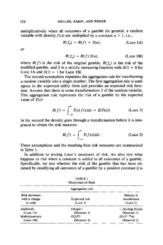
multiplicatively when all outcomes of a gamble (in general, a random variable with densityf(x)) are multiplied by a constant OL > 1, i.e.,
mJ = R(f) + St47 (Lute 1A)
or
R(f,) = R(f) S(4, (Lute 1M)
where R(f) is the risk of the original gamble, R(f,) is the risk of the modified gamble, and S is a strictly increasing function with S(1) = 0 for Lute 1A and S(1) = 1 for Lute 1M.
The second assumption stipulates the aggregation rule for transforming a random variable into a single number. The first aggregation rule is anal- ogous to the expected utility form and provides an expected risk func- tion. Assume that there is some transformation T of the random variable. This aggregation rule represents the risk of a gamble by the expected value of T(x):
R(f) = I
m T(x) f (x)dx = E(T(x)). (Lute 3)
-cc
In the second the density goes through a transformation before it is inte- grated to obtain the risk measure:
R(f) = I
- Ttf (x))dx. (Lute 2) --m
These assumptions and the resulting four risk measures are summarized in Table 1.
In addition to testing Lute’s measures of risk, we also test what happens to risk when a constant is added to all outcomes of a gamble. Specifically, we test whether the risk of the gamble that has been ob- tained by modifying all outcomes of a gamble by a positive constant p is
TABLE 1 MEASURES OF RISK
Aggregation rule
Risk increases with a change
in scale Expected risk
(Lute 3)
Density is transformed
(Lute 2)
Additively E(logixl) (Lute IA) (Measure 3)
Multiplicatively E(IX?) (Lute 1M) (Measure 4)
- Ifl4b3m))dx (Measure 1)
Jfl.x)(’ - %ix (Measure 2)
PERCEIVED RISKINESS OF GAMBLES 117
an additive or multiplicative function of the risk of the original gamble and p:
w-9 = R(f) + S(P),
or
where R(fa) is the risk of the modified gamble, and S(p) is a strictly decreasing function. An implication of the multiplicative form, taken in conjunction with the expectation principle (Lute 3), is that the risk of a gamble is the expectation of an exponential functional. This model is rep- resented by
m R(f) =
I K ecxf(x)dx,
-cc
where
K > 0, c < 0, or K < 0, c > 0.
The proof for this model is given in Satin (1984). The additive form is inappropriate as it leads to expected outcome as the measure of risk.
3. EMPIRICAL STUDY
3.1. Setting and Task
The empirical tests reported here were carried out in the U.S. and Ger- many using graduate business students. Both the U.S. and the German subjects answered identical questions, except for the German subjects the outcomes were converted into Deutsch Marks and the questionnaires were translated into German. Since the tests in the U.S. and Germany are replicates of each other, we will not make a distinction between the two until the results section, where the results will be reported sepa- rately.
The subjects were randomly divided into two groups. Each group met on 2 days. The first day they did the entire experiment. A few days later they repeated the same tasks. The experiment took approximately % h on each day. Among the U.S. subjects, 37 Group I and 38 Group II subjects completed both days in the study. Thirty-three German Group I subjects and 33 German Group II subjects completed the study.
Both groups received a three-part questionnaire preceded by a page of instructions. The general instructions given to all subjects are in Fig. 1. Subjects were requested sometimes to make paired comparison judg- ments of the relative riskiness of two gambles and at other times were told to rank order nine gambles by their riskiness.
118 KELLER, SARIN, AND WEBER
The attitudes toward risk implied by managerial and societal policies and decisions are of considerable concern to scholars of decision making. As part of a study of risk attitudes, I’m interested in knowing your perception of the relative riskiness of simple options.
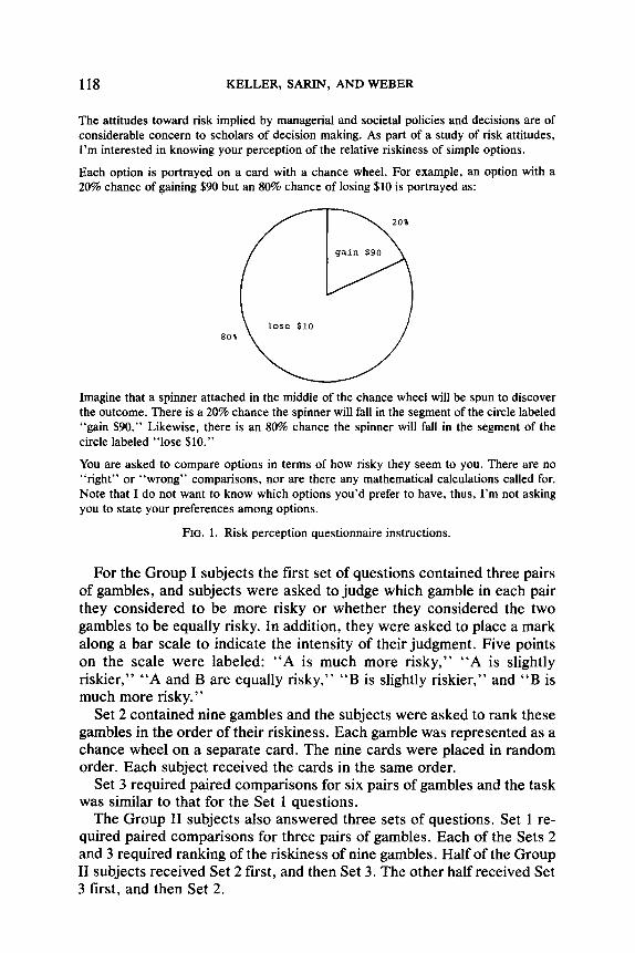
Each option is portrayed on a card with a chance wheel. For example, an option with a 20% chance of gaining $90 but an 80% chance of losing $10 is portrayed as:
80%
Imagine that a spinner attached in the middle of the chance wheel will be spun to discover the outcome. There is a 20% chance the spinner will fall in the segment of the circle labeled “gain $90.” Likewise, there is an 80% chance the spinner will fall in the segment of the circle labeled “lose $10.”
You are asked to compare options in terms of how risky they seem to you. There are no “right” or “wrong” comparisons, nor are there any mathematical calculations called for. Note that I do not want to know which options you’d prefer to have, thus, I’m not asking you to state your preferences among options.
For the Group I subjects the first set of questions contained three pairs of gambles, and subjects were asked to judge which gamble in each pair they considered to be more risky or whether they considered the two gambles to be equally risky. In addition, they were asked to place a mark along a bar scale to indicate the intensity of their judgment. Five points on the scale were labeled: “A is much more risky,” “A is slightly riskier,” “ A and B are equally risky,” “B is slightly riskier,” and “B is much more risky.”
Set 2 contained nine gambles and the subjects were asked to rank these gambles in the order of their riskiness. Each gamble was represented as a chance wheel on a separate card. The nine cards were placed in random order. Each subject received the cards in the same order.
Set 3 required paired comparisons for six pairs of gambles and the task was similar to that for the Set 1 questions.
The Group II subjects also answered three sets of questions. Set 1 re- quired paired comparisons for three pairs of gambles. Each of the Sets 2 and 3 required ranking of the riskiness of nine gambles. Half of the Group II subjects received Set 2 first, and then Set 3. The other half received Set 3 first, and then Set 2.
PERCEIVED RISKINESS OF GAMBLES 119
No subject reported any difficulty in understanding the questions. One U.S. subject’s results were discarded because of not participating on both days of the experiment. In addition, one U.S. and one German sub- ject were discarded because they did not provide the ranking of the lot- teries and instead divided the nine gambles into three risk classes.
3.2. Experimental Design and Tests of Risk Measures
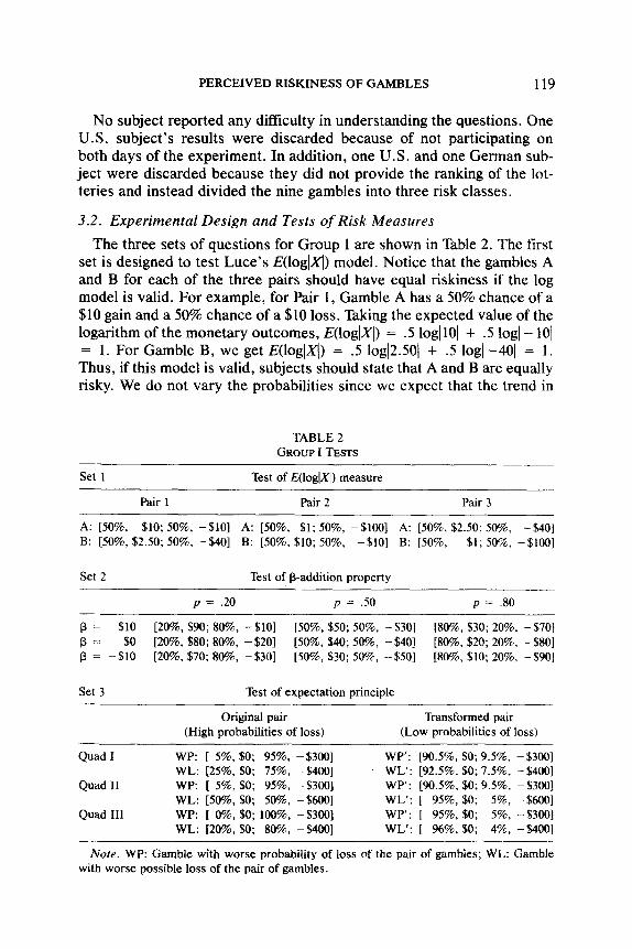
The three sets of questions for Group I are shown in Table 2. The first set is designed to test Lute’s E(log(XI) model. Notice that the gambles A and B for each of the three pairs should have equal riskiness if the log model is valid. For example, for Pair 1, Gamble A has a 50% chance of a $10 gain and a 50% chance of a $10 loss. Taking the expected value of the logarithm of the monetary outcomes, E(iogjX() = .5 log(lOl + .5 log\ - 101 = 1. For Gamble B, we get E(loglx() = .5 log12.50/ + .5 log1 -401 = 1. Thus, if this model is valid, subjects should state that A and B are equally risky. We do not vary the probabilities since we expect that the trend in
Note. WP: Gamble with worse probability of loss of the pair of gambles; WL: Gamble with worse possible loss of the pair of gambles.
120 KELLER, SARIN, AND WEBER
subjects’ judgments will be the same for probabilities different from 5. The gambles in Set 2 are designed using the form
b, a($40 d-
‘-p + P); 1 - p, a( -$40 P P J- 1-P
+ PH.
The mean for each gamble of this form is C@ and the variance is 1600~~~. For the nine gambles in Set 2, (Y = 1. Thus, the mean for each gamble is p and the variance is a constant 1600. This set will show the effect of adding p on the riskiness of gambles. Using conjoint analysis (see Krantz, Lute, Suppes & Tversky, 1971), we can also test whether the impact of p is multiplicative. In addition, we can test the mean-variance model of Pollatsek and Tversky (1970) and evaluate the impact of skew- ness on risk judgments.
The six pairs of gambles in Set 3 are designed to test the expectation principle (Lute 3). The strategy used here is similar to that used by Kah- neman and Tversky (1979) to test the substitution principle of expected utility theory. The first quadruple of gambles (QUAD I) consists of an “original pair” of gambles and a “transformed pair” of gambles. In the original pair of gambles, the “WP” gamble has the worse probability of loss, since there is a 95% chance of losing $300 compared with the 75% chance of loss with the “WL” gamble. The “WL” gamble has the worse possible loss of $400. The transformed pair of gambles is constructed by taking a A probability of getting the original pair of gambles and a 1-A probability of getting $0, In the first and second quadruples of gambles, A = .lO, and in the third quadruple, A = .05. To be consistent with the expectation principle, if the WP gamble is riskier than the WL gamble in an original pair of gambles, then for the corresponding transformed pair of gambles, WP’ should also be riskier than WL’. The worse probability and worse loss gambles were put in random order in each pair and all subjects received the six pairs of gambles in the same order.
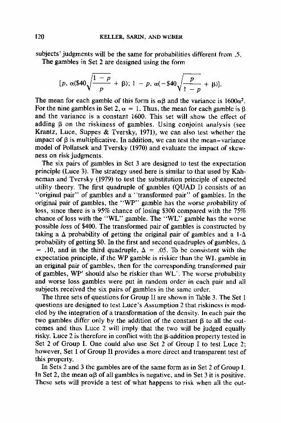
The three sets of questions for Group II are shown in Table 3. The Set 1 questions are designed to test Lute’s Assumption 2 that riskiness is mod- eled by the integration of a transformation of the density. In each pair the two gambles differ only by the addition of the constant p to all the out- comes and thus Lute 2 will imply that the two will be judged equally risky. Lute 2 is therefore in conflict with the p-addition property tested in Set 2 of Group I. One could also use Set 2 of Group I to test Lute 2; however, Set 1 of Group II provides a more direct and transparent test of this property.
In Sets 2 and 3 the gambles are of the same form as in Set 2 of Group I. In Set 2, the mean @ of all gambles is negative, and in Set 3 it is positive. These sets will provide a test of what happens to risk when all the out-
PERCEIVED RISKINESS OF GAMBLES 121
TABLE 3 GROUP II TESTS
Set 1
Pair I
Test of Lute’s assumption 2
Pair 2 Pair 3
P = 0: w% $40; 50%. -%401 p = 30: [SO%, $70; 50%. -$lO] p = 0: [50%. $40; 50%, -$40] P = 30: [50%, $70; 50%. -$lOl p = -30: [50%, $10; 50%, -$70] p = -30: [50%, $10; 50%, -$70]
Tests of cr-multiplication properties (Lute IA and IM)
comes of a gamble are multiplied by a constant (Y (thus testing Lute IA and IM).
Taken together, this study will provide a test of the measures of risk proposed by Lute, a replication of the Coombs and Bowen (1971a, 1971b) test of the mean-variance model, and a test of the impact on risk of adding p to all outcomes of a gamble. Our aim here is to identify those properties of risk that consistently hold for a wide majority of subjects.
4. RESULTS
In this section we report the results of our study in the same order as we discussed our experimental design above. These results are based on subjects’ responses on the first day. The responses for the second day are used only to provide a consistency measure.
4.1, Results for Group I
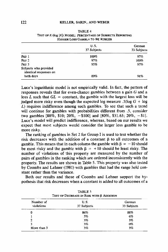
In Group I, Set 1, it was clear that subjects did not consider the two gambles in any of the three pairs to be equally risky. In fact, they consis- tently regarded the gamble with the higher loss amount to be more risky. The percentage of subjects who regarded the gamble with the higher loss amount to be riskier is reported in Table 4. The percentage of subjects who showed consistent judgments for all three pairs of gambles on both days is also shown.
These results clearly indicate that for the gambles we considered,
Lute’s logarithmic model is not empirically valid. In fact, the pattern of responses reveals that for even-chance gambles between a gain G and a loss L such that GL = constant, the gamble with the largest loss will be judged more risky even though the expected log measure .5(log G + log L) requires indifference among such gambles. To see that such a trend will continue for gambles with probabilities different from .5, consider two gambles [80%, $10; 20%, -$lOO] and [80%, $31.63; 20%, -$l]. Lute’s model will predict indifference, whereas, based on our results we expect that most subjects would consider the larger loss gamble to be more risky.
The ranking of gambles in Set 2 for Group I is used to test whether the risk decreases with the addition of a constant p to all outcomes of a gamble. This means that in each column the gamble with l3 = - 10 should be most risky and the gamble with p = + 10 should be least risky. The number of violations of this property are measured by the number of pairs of gambles in the ranking which are ordered inconsistently with the property. The results are shown in Table 5. This property was also tested by Coombs and Lehner (1981) with gambles that had the range held con- stant rather than the variance.
Both our results and those of Coombs and Lehner support the hy- pothesis that risk decreases when a constant is added to all outcomes of a
TABLE 5 TESTOFDECREASEINRISKWITHP ADDITION
Number of violations
U.S. 37 Subjects
German 33 Subjects
0 86% 88% 1 5% 6% 2 3% 3% 3 3% 0% More than 3 3% 3%
PERCEIVED RISKINESS OF GAMBLES 123
gamble. If we define the risk of a gamble to be R(f) and R(fs) to be the risk of the modified gamble after p is added to all outcomes of the original gamble, then we have shown (see Table 5) that
KP) 22 w-9, for all pr S p2.
However, we need to show whether
KP) = Wf) S(P) or w-1 + w9.
The additive assumption is ruled out since it implies that the risk measure is simply the expected value of the gamble. The multiplicative assump- tion implies the exponential model which takes into account the entire probability distribution in defining a risk measure. This seems empirically more appealing because Coombs and Bowen (1971a), and subsequently Coombs and Lehner (1981), have shown that even the first three mo- ments (expected value, variance, and skewness) of a distribution are not sufficient to describe riskiness,
Using the theory of conjoint analysis we need to test independence and the double cancellation condition (Krantz et al., 1971). Independence re- quires that the ranking in each row (as the probability of gain varies) and in each column (as the amount p added to all outcomes varies) be iden- tical. We did not test for double cancellation directly. Instead, using the strategy of Coombs and Lehner (1983), we directly tested for additivity.
To test additivity for those who were independent, we used a 0- 1 in- teger program. The output of this program is the number of permutation changes that are required in neighbor pairs in the rankings to make the entire matrix consistent with additivity. It should be noted that this test of additivity is appropriate since after the logarithmic transformation the multiplicative model is indeed additive. We also tested for sign depen- dence to ensure that a subject who violated independence but satisfied sign dependence is not labeled inconsistent with the multiplicative model. However, no subject satisfied sign dependence.
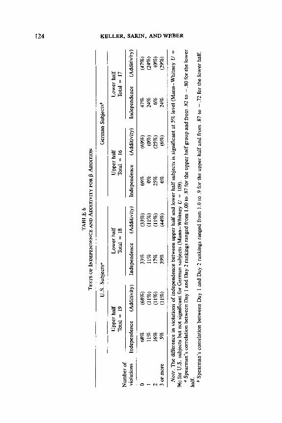
In our data approximately 50% of the subjects had at least one viola- tion of both independence and additivity. Following Coombs and Lehner (1981), we divided the subjects into approximately equal halves based on the correlation of their rankings between Day 1 and Day 2. The subjects in the upper half group who were relatively more consistent than the sub- jects in the lower half group could thus be studied separately with respect to their violation of the independence and additivity properties. The re- sults are reported in Table 6.
The first result we observe from Table 6 is that 69% of the subjects who were relatively consistent between Day 1 and Day 2 satisfied additivity. Notice that if a perfectly consistent subject switches a sixth ranked gamble with an eighth ranked gamble while leaving all other gambles at
TABL
E 6
TEST
SOFI
ND
EPEN
DEN
CEA
ND
ADD
ITIV
ITYF
OR
P AD
DIT
ION
U.S
. Su
bjec
tsa
Ger
man
Sub
ject
@
Upp
er h
alf
Tota
l =
19
Num
ber
of
viol
atio
ns
Inde
pend
ence
(A
dditi
vity
)
0 68
%
(68%
) 1
11%
(1
1%)
2 16
%
(11%
) 3
or m
ore
5%
(11%
)
Low
er
half
Tota
l =
18
Inde
pend
ence
(A
dditi
vity
)
33%
(3
3%)
11%
(1
1%)
17%
(1
1%)
3%
(44%
)
Upp
er h
alf
Low
er
half
F To
tal
= 16
To
tal
= 17
.F
In
depe
nden
ce
(Add
itivi
ty)
Inde
pend
ence
(A
dditi
vity
) U
J
69%
(6
9%)
47%
ii
(47%
) ,z
0%
(0
%)
24%
(2
4%)
25%
(2
5%)
6%
(0%
) %
6%
(6
%)
24%
(2
9%)
Not
e. T
he d
iffer
ence
in
viol
atio
ns
of in
depe
nden
ce b
etw
een
uppe
r ha
lf an
d lo
wer
hal
f su
bjec
ts
is s
igni
fican
t at
5%
leve
l (M
ann-
Whi
tney
U
=
i 96
) for
U.S
. su
bjec
ts b
ut n
ot s
igni
fican
t fo
r G
erm
an s
ubje
cts
(Man
n-W
hitn
ey
II =
109)
. E
0 Sp
earm
an’s
cor
rela
tion
betw
een
Day
1 a
nd D
ay 2
rank
ings
ran
ged
from
1 .O
O to
.87
for
the
uppe
r ha
lf gr
oup
and
from
.82
to -
30
for
the
low
er
half.
b
Spea
rman
’s c
orre
latio
n be
twee
n D
ay 1
and
Day
2 ra
nkin
gs r
ange
d fro
m 1
.0 to
.9
for
the
uppe
r ha
lf an
d fro
m .
87 to
- .
72 fo
r th
e lo
wer
hal
f.
PERCEIVED RISKINESS OF GAMBLES 125
their original ranking, then he incurs three violations. If we disallow all such violations but do allow at the most two mistakes in the ranking of adjacent pairs, then more than 90% of the subjects in the upper half group, and more than 75% of all subjects, conform with additivity.’
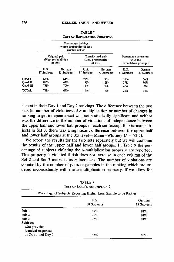
In Set 3, the expectation principle was tested. The results, reported in Table 7, show that only about one-third of the subjects provided judg- ments consistent with the expectation principle (Lute 3). Further, the pattern of violation was systematic. For each quadruple there are nine possible combinations of responses and three of these combinations (WP and WP’ riskier, WL and WL’ riskier, or WP and WL equally risky, as well as WP’ and WL’ equally risky) are consistent with the expected risk principle. Actual responses of the subjects for each pair were signifi- cantly different (at the 1% level) from the equal likelihood pattern of re- sponses, showing a systematic pattern. This pattern, loosely speaking, is that when the probability of loss is high, then the gamble with the worse probability of loss is considered more risky (as shown in Table 7). How- ever, when the probability of loss is low, then the gamble with the higher loss amount is judged to be more risky. Thus, attention may be shifting from probability of loss to loss amount L when a gamble [p, $0; l-p, L] is transformed into a gamble [I-A(l-p), $0; A(l-p), L], 0 < A < 1, causing a reversal in risk judgments for low values of A.
4.2. Results for Group II
In Set 1, the gambles in each of the three pairs should be regarded equally risky if Lute’s Assumption 2 (that riskiness is modeled by the integration of a transformation of the density) is valid. The results in Table 8 show that subjects consistently violated this assumption as they regarded the higher loss gamble to be more risky.
Set 2 and Set 3 for Group II require identical analysis since the objec- tive in both sets is to examine the impact of (Y multiplication on risk. In Set 2 the means al3 of the gambles are negative (p = - 10) and in Set 3 they are positive (p = + 10). We had thought a priori that the results might be different for the two sets. We carried out the test of the a-multi- plication property, independence, and additivity for the two sets sepa- rately. Within each set the group was divided into two equal halves- with the upper half consisting of subjects who were relatively more con-
i Though our purpose was to investigate additivity, this data can also be used to demon- strate the influence of skewness on riskiness. Further analysis of the data showed that only three U.S. and three German subjects considered the symmetric gambles (middle column) to be riskier than the skewed gambles in the same row even though all three gambles in a row had equal mean and variance. This supports the results of Coombs and Bowen (1971a) that subjects’ judgments are influenced by skewness, and thus the mean-variance model is not empirically valid.
sistent in their Day 1 and Day 2 rankings. The difference between the two sets (in number of violations of cx multiplication or number of changes in ranking to get independence) was not statistically significant and neither was the difference in the number of violations of independence between the upper half and lower half groups in each set (except for German sub- jects in Set 3, there was a significant difference between the upper half and lower half groups at the .05 level-Mann-Whitney U = 72.5).
We report the results for the two sets separately but we will combine the results of the upper half and lower half groups. In Table 9 the per- centage of subjects violating the a-multiplication property are reported. This property is violated if risk does not increase in each column of the Set 2 and Set 3 matrices as cx increases. The number of violations are counted by the number of pairs of gambles in the ranking which are or- dered inconsistently with the o-multiplication property. If we allow for
TABLE 8 TESTOFLUCE’SASSUM~ION~
Percentage of Subjects Reporting Higher Loss Gamble to be Riskier
U.S. 38 Subjects
German 33 Subiects
Pair 1 Pair2 Pair3 Subjects
who provided identical responses on Day 1 and Day 2
87% 94% 95% 94% 92% 91%
82% 85%
PERCEIVED RISKINESS OF GAMBLES 127
TABLE 9 TEST OF INCREASE IN RISK WITH cx MULTIPLICATION
Number of violations
U.S. German 38 Subjects 33 Subjects
Set 2 Set 3 Set 2 Set 3 p= -10 p= +10 p= -10 p= +to
0 I 2 3 4 or more
42% 45% 55% 55% 21% 5% 12% 6%
8% 8% 9% 6% 13% 16% 9% 9% 16% 26% 15% 24%
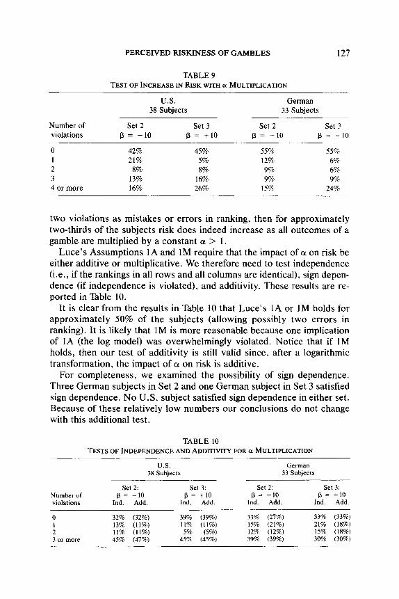
two violations as mistakes or errors in ranking, then for approximately two-thirds of the subjects risk does indeed increase as all outcomes of a gamble are multiplied by a constant cr. > 1.
Lute’s Assumptions 1A and 1M require that the impact of (Y on risk be either additive or multiplicative. We therefore need to test independence (i.e., if the rankings in all rows and all columns are identical), sign depen- dence (if independence is violated), and additivity. These results are re- ported in Table 10.
It is clear from the results in Table 10 that Lute’s 1A or 1M holds for approximately 50% of the subjects (allowing possibly two errors in ranking). It is likely that IM is more reasonable because one implication of IA (the log model) was overwhelmingly violated. Notice that if 1M holds, then our test of additivity is still valid since, after a logarithmic transformation, the impact of cr on risk is additive.
For completeness, we examined the possibility of sign dependence. Three German subjects in Set 2 and one German subject in Set 3 satisfied sign dependence. No U.S. subject satisfied sign dependence in either set. Because of these relatively low numbers our conclusions do not change with this additional test.
TABLE 10 TESTS OF INDEPENDENCE AND ADDITIVITY FOR a MULTIPLICATION
These data were also used to verify that risk judgments are influenced by skewness since, in spite of equal variance in the three columns for each row, the symmetric gamble (middle column) was regarded as being more risky than the asymmetric gambles (first and third columns) by only 18% of the subjects.
We now compare the relative conformance with the properties that risk decreases as p is added to all outcomes of a gamble and that risk in- creases as all outcomes are multiplied by a. From Tables 5 and 9, we note that only 14% of the U.S. subjects and 12% of the Germans violated the P-addition property, in contrast with 5% of the U.S. subjects and 45% of the German subjects who violated the a-multiplication property. The dif- ference in the distribution of the number of violations of the P-addition and a-multiplication properties is significant at the 1% level (Mann- Whitney U tests).
Similarly, conformance with additivity is greater for the l3 factor than for the (Y factor (Tables 6 and 10). Only 49% of the U.S. subjects and 42% of the Germans violated the additivity of R(f) and S(p), in contrast with the 64% of the U.S. subjects and 70% of the German subjects who vio- lated the additivity of R(f) and S(a).
5. CONCLUSIONS AND DIRECTIONS FOR FURTHER RESEARCH
In our empirical study we observed remarkable consistency in the risk judgments of the U.S. and German subjects. This suggests that, for the type of gambles we considered, subjects have a definite notion about the perceived riskiness of gambles. But, can this notion be captured by a mathematical formula, even for well-defined gambles?
Lute (1980, 1981) proposed four measures of risk. His Measures 1 and 2 (see Table 1) are clearly inappropriate, as both of these measures re- quire that risk should not change if we add a constant p to all outcomes of a gamble. We find clear evidence that risk decreases with addition of p. Lute himself (1980, p. 222) notes this problem, and our data convincingly confirm his doubt.
Lute’s logarithmic Measure 3 is also deficient, since almost all the subjects exhibit a clear difference in the perceived riskiness of gambles that ought to be judged equally risky if Measure 3 is true.
Lute’s Measure 4 (the expectation of the absolute value of the out- comes raised to a parameter G) seems to have more promise than his other three measures. Lute and Weber (forthcoming) recently proposed a variant of this most promising measure.
Because of its nice mathematical properties, the expectation principle, originally proposed for risk by Huang (1971), has been retained by many researchers in their axiom systems. Recently, Kahneman and Tversky
PERCEIVED RISKINESS OF GAMBLES 129
(1979) and others have questioned the empirical-validity of the expecta- tion principle for predicting choices. The results of this study suggest that the principle may not be valid for risk judgments either.
Our results provide some insights into how perceived risk varies with the probabilities and outcomes. First, we note that the p-addition prop- erty is empirically appealing. Second, the expectation principle seems to be inappropriate. Third, the probability of loss seems to have relatively more influence on risk perception when this probability is high, and the amount of loss has more influence on risk perception when this proba- bility is low. [Further research, following the approach used in Levin, Louviere, Schepanski, and Norman (1983) and Hammond, McClelland, and Mumpower (1980), is needed to determine the relative influence of these factors on risk judgments.] Fourth, the skewed gambles are more risky than the corresponding symmetric gambles of equal mean and vari- ance. It would be interesting to verify these results for different stimuli such as health consequences or multiple outcome gambles.
The challenge is to incorporate these observations into a mathematical rule. We believe that it is unlikely that a mathematical rule will capture all aspects of risk perception in real decision situations that are character- ized by ambiguity, context and framing effects, aspiration or target levels, and other situation-specific issues. However, as a first approximation, even for well-defined gambles, an attempt to discover an empirically valid mathematical rule is worthwhile. Fishburn (1982, 1984), Lute and Weber (1984), and Lopes (1984) provide a start in this direction.
We are pursuing two directions of research on this topic. One is to examine the determinants of perceived risk in situations that may be closer to real operational contexts. The impacts of ambiguity, uncertainty about the probabilities, single-stage vs. two-stage gambles, target levels, etc., on perceived risk need to be examined. The second direction of research is to integrate risk perception with preference. It is possible that a better understanding of a subject’s choices in risky situations is achieved when one explicitly accounts for risk perception in the choice model. If ambiguous gambles are perceived to be more risky, then the Elisberg paradox (1961)-in which gambles with known probabilities are preferred over gambles with ambiguous probabilities-can be explained by a two-attribute choice model where the tirst attribute is the utility or value of the outcomes and the second attribute is the riskiness of the gamble.
In conclusion, while perceived risk is as yet a vaguely defined and somewhat poorly understood concept, we are encouraged by the consis- tency of subjects’ responses. Our results, while largely negative with re- spect to Lute’s models, do support his speculation, “then we know we must turn to more complex theory.” Further, these results provide some
130 KELLER, SARIN, AND WEBER
necessary conditions that a new theory or extension of Lute’s measures must satisfy.
REFERENCES Coombs, C. H. (1%9). Portfolio theory: A theory of risky decision making. In La decision.
Paris: Centre National de la Recherch Scientifique. Coombs, C. H., & Bowen, J. N. (197la). A test of VE-theories of risk and the effect of the
central limit theorem. Acta Psychologicn, 35, 15-28. Coombs, C. H., & Bowen, J. N. (197lb). Additivity of risk in portfolios. Perception and
Psychophysics, 10, 43-46. Coombs, C. H., & Huang, L. C. (1970a). Polynomial psychophysics of risk. Journal of
Mathematical Psychology, 7, 317-338. Coombs, C. H., Huang, L. C. (1970b). Tests of a portfolio theory of risk preference.
Journal of Experimental Psychology, 85, 23-29. Coombs, C. H., & Lehner, P. E. (1981). Evaluation of two alternative models for a theory
of risk. I. Journal of Experimental Psychology, Human Perception and Performance, 7, 1110-1123.
Coombs, C. H., & Lehner, P. E. (1983). Conjoint design and analysis of the bilinear model: An application to judgments of risk. University of Michigan.
Ellsberg, D. (1961). Risk, ambiguity, and the Savage axioms. Qunrterly Journal of Eco- nomics, 75, 643-649.
Fishbum, P C. (1982). Foundations of risk measurement. II. Effects of gains on risk. Journal of Mathematical Psychology, 25, 226-242.
Fishbum, P C. (1984). Foundations of risk measurement. I. Risk as probable loss. Munage- ment Science, 30, 396-406.
Hammond, K. R., McClelland, G. H., & Mumpower, J. (1980). Human judgment and deci- sion making: Theories, methods, and procedures. New York: Hemisphere/Praeger.
Huang, L. C. (1971). The expected risk function (Michigan Mathematical Psychology Pro- gram Report 71-6). Ann Arbor: University of Michigan.
Kahneman, D. H., & Tversky, A. (1979). Prospect theory: An analysis of decision under risk. Econometrica, 47, 263-290.
Krantz, D. H., Lute, R. D., Suppes, P., & Tversky, A. (1971). Foundutions of measure- ment. I. New York: Academic Press.
Levin, I., Louviere, J. J., Schepanski, A. A., & Norman, K. L. (1983). External validity tests of laboratory studies of information integration. Organizational Behavior and Human Performance, 31, 173-193.
Lopes, L. (1984). Risk and distributional inequality. Journal of Experimental Psychology: Human Perception and Performance, 10, (4). 465-485.
Lute, R. D. (1980, 1981). Several possible measures of risk. Theory and Decision, 12, 217-228; Correction, 13, 381.
Lute, R. D., & Weber, E. U. (forthcoming). An axiomatic theory of conjoint, expected risk. Journal of Mathematical Psychology.
Pollatsek, A., & Tversky, A. (1970). A theory of risk. Journal of Mathematical Psychology, 7, 540-553.
Sarin, R. K. (1984). Some extensions of Lute’s measures of risk (Working Paper). Graduate School of Management, University of California-Los Angeles.
Weber, E. (1984). Combine and conquer: A joint application of conjoint and functional approaches to the problem of risk measurement. Journal of Experimental Psychology, Human Perception and Performance, 10, 179- 194.