International Journal of DIGITAL TECHNOLOGY & ECONOMY Volume 1 | Number 1 | 2016 | 1 | Machine learning model for early detecon of higher educaon students that need addional aenon in introductory programming courses Goran Đambić Mirjana Krajcar Daniel Bele University College Algebra, Zagreb, Croaa University College Algebra, Zagreb, Croaa University College Algebra, Zagreb, Croaa [email protected][email protected][email protected]Abstract: Not all higher educaon students who enroll in introductory pro- gramming course successfully finish it, in parcular if their major is not computer programming or computer science. From empirical evidence collected at the University College Algebra we have concluded that such students can be given a beer passing chance if they are idenfied early in the semester and given addional aenon in form of extra hours in classroom, guided by mentors. The challenge lies in being able to disn- guish such students as early as possible so they can benefit from addion- al learning hours before the final exams. This paper proposes one such possible criterion: we develop a machine learning model based on previ- ous generaons of students and use it for current students to calculate the probability of finishing the course unsuccessfully. Such students are then classified as »requiring extra aenon«. Keywords: machine learning, model, early detecon, logisc regression, higher educa- on student, addional aenon Original scienfic paper / Izvorni znanstveni rad Manuscript received: 2015-09-08 Revised: 2016-05-25 Accepted: 2016-05-25 Pages: 1 - 11
Transcript
International Journal of DIGITAL TECHNOLOGY & ECONOMY Volume 1 | Number 1 | 2016
| 1 |
Machine learning model for early detection of higher education students that need additional attention in introductory
Abstract: Not all higher education students who enroll in introductory pro-gramming course successfully finish it, in particular if their major is not computer programming or computer science. From empirical evidence collected at the University College Algebra we have concluded that such students can be given a better passing chance if they are identified early in the semester and given additional attention in form of extra hours in classroom, guided by mentors. The challenge lies in being able to distin-guish such students as early as possible so they can benefit from addition-al learning hours before the final exams. This paper proposes one such possible criterion: we develop a machine learning model based on previ-ous generations of students and use it for current students to calculate the probability of finishing the course unsuccessfully. Such students are then classified as »requiring extra attention«.
Original scientific paper / Izvorni znanstveni radManuscript received: 2015-09-08
Revised: 2016-05-25Accepted: 2016-05-25
Pages: 1 - 11
www.eLeadership.mba
In Cooperation with faculties from Kelley School of Business, Indiana University
“Leadership is the capacity to translate vision into reality.”
Warren Bennis
eLeadership MBADoing Business in Digital Economy
Machine learning model for education, Đambić et al. [1-11]
| 2 |
INTRODUCTIONFor some higher education students, basic programming concepts are not easy to grasp [3]. That especially holds true for students whose major is not in field of computer science. Such students enroll in introductory courses in programming either willingly, by choosing it as an optional course, or mandatory, by having such class in mandatory list of classes for their study program. In many cases, such entry-level programming course is considered a basic building block course for computer science study programs, very similar to mathematics, electrical engineering, digital electronics or computer net-works basics.At our university, Introduction to programming is a basic course for all technical study programs (Software Engineering, System Engineering and Multimedia Engineering) and is taught in first semester, mandatory for all students. The passing rate of all enrolled students in the last three academic years is roughly 60%, which is a bit, but not much, lower than the approximate 70% reported in [1]. Passing rate was even lower before that, being around 50%. The main reason behind the increase in passing rate three years ago was the introduc-tion of several additional and mandatory classes for students who exhibited problems in grasping programming concepts at the beginning of the semester. Such students were pointed to mentors who worked with them through the rest of the semester and by do-ing that, passing rate went up. Additional classes were designed as a mixture of auditory exercises and consultations, rather informally structured and led by student mentors.Although these additional activities gave results, we faced the same challenge every year – how to identify students that are going to have problems with passing Introduc-tion to programming and how to do that early in the semester. Obviously, it is very easy to identify such students a posteriori, but if we were to help them in time, such identi-fication has to be made as early as possible. One approach was asking students if they feel confident that they would master taught concepts or do they think they could benefit from additional exercises. Early in the first semester, very few students were ready to accept additional exercises, especially man-datory ones. Other approaches would rely on more formal measures. We learned that the earliest possible point in which we had enough data to predict if student is going to have problems with programming or not was right after the first colloquium, mainly based on students’ success on the exam. But even then, it was not clear where to put a threshold that will reasonably divide students who might succeed and those who might fail. In different years different methods were used, some based on cumulative number of points from the exam regardless of the learning outcomes, some based on number of passed or failed learning outcomes.It was recognized that one method should be envisioned that will be used to, as best as possible, predict whether students will fail the course or not. The purpose of this paper is to propose such a method in the form of a machine learning model. This model will be trained on students from the previous year and will be used to estimate current year
International Journal of DIGITAL TECHNOLOGY & ECONOMY Volume 1 | Number 1 | 2016
| 3 |
students’ chance of failing the course. Student that will be marked as »probably will fail« will then be selected for additional learning activities.
DEFINITION OF THE MODELIn this section, a machine learning model and its building blocks are defined. That model will be used in following sections in order to identify students who might have problems getting their passing grade for Introduction to programming course.
STATE OF PLAY AT OUR UNIVERSITY
At our university, each semester is divided in three parts, each lasting for five weeks of lectures and exercises. After each part, a colloquium is held in order to validate stu-dents’ knowledge of learning outcomes taught in just finished part of semester. The third colloquium is also considered a final exam and students can get their passing grade at that time. If not, additional exam term is available approximately two weeks after that, and additional three exam terms are available through the rest of that academic year. Students not getting their passing grade in one year from course start are consid-ered as failed and must reenroll to that course next year.During the semester, three quizzes are held, one in each part of the semester. In the same manner, three homework assignments are given to students, also one in each part of the semester.
CHOICE OF FEATURES
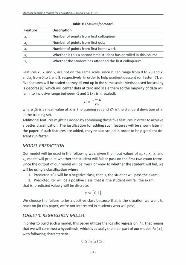
Bearing in mind the imperative of being able to early in the semester decide who should get additional attention, inputs for a model must be chosen appropriately. That means that we cannot wait until the end of the semester in order to get precise data on stu-dents’ collected points, but also means that we cannot create model based on, for ex-ample, three weeks of the semester. From previously described methods of validation, it is obvious that the first point in the semester at which we can have sufficient information for building a model can be no sooner than after the first five weeks. At that point, students will have accumulated points from first colloquium, first quiz and first homework. Those accumulated points and the way they were accumulated will be used as features for our model, together with two additional features, as shown in table 1.Feature x4 can be valued 0 or 1, depending on whether is this first time the student has enrolled in this course (value 0) or the second time (value 1). Feature x5 can also be val-ued 0 or 1, depending on whether student did actually come to write first colloquium (value 1) or not (value 0). It is used to distinguish between situations in which student wrote colloquium and achieved 0 points and those in which student didn’t even come to colloquium.
Machine learning model for education, Đambić et al. [1-11]
| 4 |
Table 1: Features for model.
Feature Descriptionx1 Number of points from first colloquiumx2 Number of points from first quizx3 Number of points from first homeworkx4 Whether is this a second time student has enrolled in this coursex5 Whether the student has attended the first colloquium
Features x1, x2 and x3 are not on the same scale, since x1 can range from 0 to 28 and x2 and x3 from 0 to 2 and 3, respectively. In order to help gradient descent run faster [7], all five features will be scaled so they all end up in the same scale. Method used for scaling is Z-scores [8] which will center data at zero and scale them so the majority of data will fall into inclusive range between -1 and 1 ( x il is xi scaled):
xx
ii
i i
vn
=-l
where in is a mean value of xi in the training set and iv is the standard deviation of xi in the training set. Additional features might be added by combining those five features in order to achieve a better classification. The justification for adding such features will be shown later in the paper. If such features are added, they’re also scaled in order to help gradient de-scent run faster.
MODEL PREDICTION
Our model will be used in the following way: given the input values of x1, x2, x3, x4 and x5, model will predict whether the student will fail or pass on the first two exam terms. Since the output of our model will be »yes« or »no« to whether the student will fail, we will be using a classification where:
1. Predicted »0« will be a negative class, that is, the student will pass the exam.1. Predicted »1« will be a positive class, that is, the student will fail the exam.
that is, predicted value y will be discrete:
,y 0 1d # -We choose the failure to be a positive class because that is the situation we want to react on (in this paper, we’re not interested in students who will pass).
LOGISTIC REGRESSION MODEL
In order to build such a model, this paper utilizes the logistic regression [4]. That means that we will construct a hypothesis, which is actually the main part of our model, h xi ^ h, with following characteristic:
h x0 1# #i ^ h
International Journal of DIGITAL TECHNOLOGY & ECONOMY Volume 1 | Number 1 | 2016
| 5 |
Strictly speaking, the output of our hypothesis should be interpreted as follows:
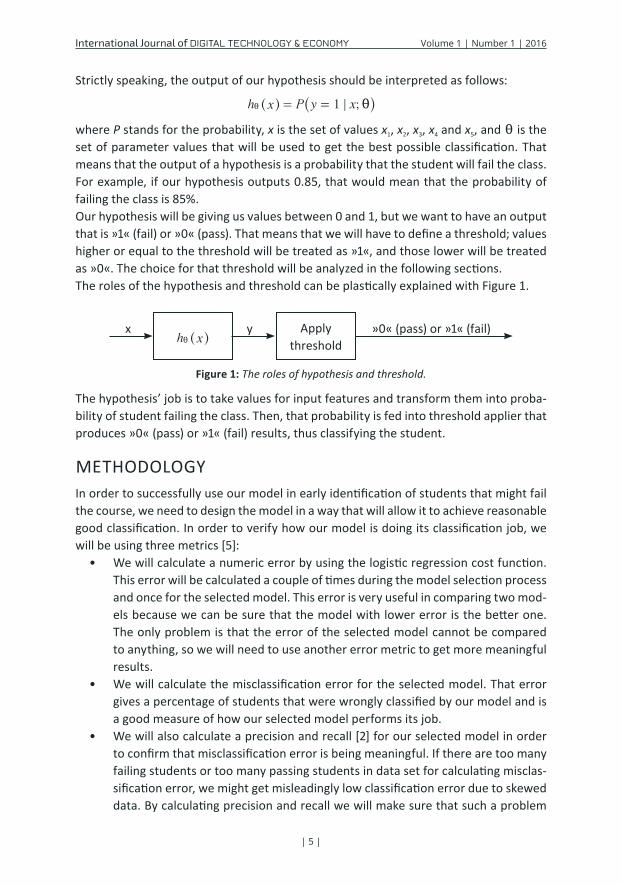
;h x P y x1 ; i= =i ^ ^h hwhere P stands for the probability, x is the set of values x1, x2, x3, x4 and x5, and i is the set of parameter values that will be used to get the best possible classification. That means that the output of a hypothesis is a probability that the student will fail the class. For example, if our hypothesis outputs 0.85, that would mean that the probability of failing the class is 85%.Our hypothesis will be giving us values between 0 and 1, but we want to have an output that is »1« (fail) or »0« (pass). That means that we will have to define a threshold; values higher or equal to the threshold will be treated as »1«, and those lower will be treated as »0«. The choice for that threshold will be analyzed in the following sections.The roles of the hypothesis and threshold can be plastically explained with Figure 1.
h xi ^ h Apply threshold
»0« (pass) or »1« (fail)x y
Figure 1: The roles of hypothesis and threshold.
The hypothesis’ job is to take values for input features and transform them into proba-bility of student failing the class. Then, that probability is fed into threshold applier that produces »0« (pass) or »1« (fail) results, thus classifying the student.
METHODOLOGYIn order to successfully use our model in early identification of students that might fail the course, we need to design the model in a way that will allow it to achieve reasonable good classification. In order to verify how our model is doing its classification job, we will be using three metrics [5]:
• We will calculate a numeric error by using the logistic regression cost function. This error will be calculated a couple of times during the model selection process and once for the selected model. This error is very useful in comparing two mod-els because we can be sure that the model with lower error is the better one. The only problem is that the error of the selected model cannot be compared to anything, so we will need to use another error metric to get more meaningful results.
• We will calculate the misclassification error for the selected model. That error gives a percentage of students that were wrongly classified by our model and is a good measure of how our selected model performs its job.
• We will also calculate a precision and recall [2] for our selected model in order to confirm that misclassification error is being meaningful. If there are too many failing students or too many passing students in data set for calculating misclas-sification error, we might get misleadingly low classification error due to skewed data. By calculating precision and recall we will make sure that such a problem
y
Machine learning model for education, Đambić et al. [1-11]
| 6 |
is not occurring. Precision and recall will also be expressed as F1score in order to get just one number which will describe the performance of our model.
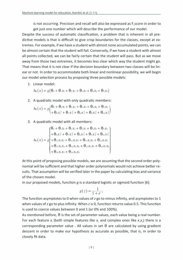
Despite the success of automatic classification, a problem that is inherent in all pre-dictive models is that is difficult to give crisp boundaries for the classes, except at ex-tremes. For example, if we have a student with almost none accumulated points, we can be almost certain that the student will fail. Conversely, if we have a student with almost all points collected, we can be fairly certain that the student will pass. But as we move away from those two extremes, it becomes less clear which way the student might go. That means that it is not clear if the decision boundary between two classes will be lin-ear or not. In order to accommodate both linear and nonlinear possibility, we will begin our model selection process by proposing three possible models:
1. Linear model:
h x g x x x x x0 1 1 2 2 3 3 4 4 5 5i i i i i i= + + + + +i _ _i i
2. A quadratic model with only quadratic members:
h x g x x x x x
x x x x x
0 1 1 2 2 3 3 4 4 5 5
6 12
7 22
8 32
9 42
10 52
i i i i i i
i i i i i=
+ + + + +
+ + + + +i _ ei o
3. A quadratic model with all members:
h x g
x x x x x
x x x x x
x x x x x x x x
x x x x x x x x
x x x x
0 1 1 2 2 3 3 4 4 5 5
6 12
7 22
8 32
9 42
10 52
11 1 2 12 1 3 13 1 4 14 1 5
15 2 3 16 2 4 17 2 5 18 3 4
19 3 5 20 4 5
i i i i i i
i i i i i
i i i i
i i i i
i i
=
+ + + + +
+ + + + +
+ + + +
+ + + +
+ +
i
J
L
KKKKKKK
_
N
P
OOOOOOO
i
At this point of proposing possible models, we are assuming that the second order poly-nomial will be sufficient and that higher order polynomials would not achieve better re-sults. That assumption will be verified later in the paper by calculating bias and variance of the chosen model.In our proposed models, function g is a standard logistic or sigmoid function [6]:
g ze11
z=+ -^ h
The function asymptotes to 0 when values of z go to minus infinity, and asymptotes to 1 when values of z go to plus infinity. When z is 0, function returns value 0.5. This function is used to coerce values between 0 and 1 (or 0% and 100%).As mentioned before, i is the set of parameter values, each value being a real number. For each feature xi (both simple features like x1 and complex ones like x1x3) there is a corresponding parameter value . All values in set i are calculated by using gradient descent in order to make our hypothesis as accurate as possible, that is, in order to closely fit data.
International Journal of DIGITAL TECHNOLOGY & ECONOMY Volume 1 | Number 1 | 2016
| 7 |
CHOOSING THE BEST MODELOur first step will be choosing one model out of three proposed model. That model will be considered a selected model for the rest of the work and other two models will be discarded. Our available data set include 181 student records from previous academic year. For the purpose of choosing the best model, we will randomly split student records into three data sets:
1. We will use 109 students (approximately 60% of existing data) as the training set.2. We will use 36 students (approximately 20% of existing data) as the cross vali-
dation set.3. We will use 36 students (approximately 20% of existing data) as the test set.
Training set will be used to calculate parameters i for each model. Parameters i must be chosen in such a way that the associated cost function ( )Jtrain i is as small as possible:
( ) log logJm
y h x y h x1 1 1traintrain
i
m
1
train
i = - - - -i i
=
_ ^ ^ _ ^hi h hi/( )Jtrain i is a standard cost function in logistic regression that calculates how big are the
discrepancies between our estimation h xi ^ h and the actual value y , and mtrain is the number of examples in the training set. Finding the exact values of the parameters i that minimize the said cost function was done by using MATLAB’s function fminunc. After we have minimized the parameters i for each model, we will be using those val-ues on cross validation data set. In this way, we are actually testing how well our model generalizes to new, previously unseen examples, that is, we are trying to use it to classi-fy students. For each model, we calculate the cost function like before, just this time on the cross validation data set, instead of the training set. The obtained cross validation costs are shown in Table 2.
Table 2: Cross validation costs for three models.
Model Cross validation costLinear model 0,184808Simple quadratic model 0,167542Full quadratic model 0,299867
Form Table 2, it is apparent that the best model to use is a simple quadratic model because it has the lowest cost, i.e. the lowest error. It seems that adding additional polynomials will not allow for better predictions because of the overfitting problem [5]. Therefore, we choose a simple quadratic model for further analysis.
REGULARIZATION OF THE MODELNow that we have chosen our model, we will try to add regularization to see if we can minimize the cost error even more and thus get a better model. The purpose on regu-larization is to find a fine balance between high biased models (ones that do not fit well
Machine learning model for education, Đambić et al. [1-11]
| 8 |
neither as train nor as cross validation models) and high variance models (ones that perfectly fit the train data but fail to generalize to cross validation data set). Regular-ization is controlled by the parameter λ. We will propose 14 different lambdas (0, 0.01, 0.02, 0.04, 0.08, 0.16, 0.32, 0.64, 1.28, 2.56, 5.12, 10.24, 20.48 and 40.96) and perform a similar set of steps like in model selection:
1. We will use the train set to minimize the parameters θ, for each λ.2. We will use the calculated parameters θ in order to calculate the cross validation
cost, for each λ.3. We will choose a single λ with the minimal cost. Other lambdas will be discarded.
It is worth mentioning that the model with λ = 0 is actually the model that does not use regularization, so we expect to get the same cost as before. Also, since we are using regularization, our training set cost function will be:
( ) log logJm
y h x y h xm
1 1 12train
train traini
j
j
nm
1
2
1
train
i m i= - - - - +i i
= =
_ ^ ^ _ ^hi h hi8 B/ /
Cost functions for the cross validation set and the test set will remain same as before. Obtained cross validation costs are shown in Table 3.
Table 3: Cross validation costs for simple quadratic model and different lambdas.
From Table 3, it is obvious that λ = 0 will yield the best results so we choose that value for λ.
VALIDATION OF THE FINAL MODELAfter completing the previous steps, we ended up with a model that we will propose as a final model for classifying students. That final model is presented with the following hypothesis:
h x g x x x x x x x x x x0 1 1 2 2 3 3 4 4 5 5 6 12
7 22
8 32
9 42
10 52i i i i i i i i i i i= + + + + + + + + + +i _ _i i
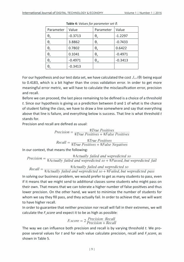
where the parameters θ have values shown in Table 4.
International Journal of DIGITAL TECHNOLOGY & ECONOMY Volume 1 | Number 1 | 2016
For our hypothesis and our test data set, we have calculated the cost ( )Jtest i being equal to 0.4183, which is a bit higher than the cross validation error. In order to get more meaningful error metric, we will have to calculate the misclassification error, precision and recall.Before we can proceed, the last piece remaining to be defined is a choice of a threshold t. Since our hypothesis is giving us a prediction between 0 and 1 of what is the chance of student failing the class, we have to draw a line somewhere and say that everything above that line is failure, and everything below is success. That line is what threshold t stands for.Precision and recall are defined as usual:
# ##Precision
True Positives False PositivesTrue Positives
=+
# ##Recall
True Positives False NegativesTrue Positives
=+
In our context, that means the following:
# # ,#
PrecisionActually failed and wepredicted so Passed but wepredicted fail
Actually failed and wepredicted so=
+
# # ,#
RecallActually failed and wepredicted so Failed but wepredicted pass
Actually failed and wepredicted so=
+
In solving our business problem, we would prefer to get as many students to pass, even if it means that we might send to additional classes some students who might pass on their own. That means that we can tolerate a higher number of false positives and thus lower precision. On the other hand, we want to minimize the number of students for whom we say they fill pass, and they actually fail. In order to achieve that, we will want to have higher recall.In order to guarantee that neither precision nor recall will fall in their extremes, we will calculate the F1score and expect it to be as high as possible:
F scorePrecision RecallPrecision Recall21
$=
+
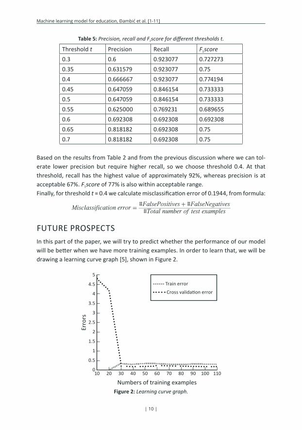
The way we can influence both precision and recall is by varying threshold t. We pro-pose several values for t and for each value calculate precision, recall and F1score, as shown in Table 5.
Machine learning model for education, Đambić et al. [1-11]
| 10 |
Table 5: Precision, recall and F1score for different thresholds t.
Based on the results from Table 2 and from the previous discussion where we can tol-erate lower precision but require higher recall, so we choose threshold 0.4. At that threshold, recall has the highest value of approximately 92%, whereas precision is at acceptable 67%. F1score of 77% is also within acceptable range.Finally, for threshold t = 0.4 we calculate misclassification error of 0.1944, from formula:
## #
Misclassification errorTotal number of test examplesFalsePositives FalseNegatives
=+
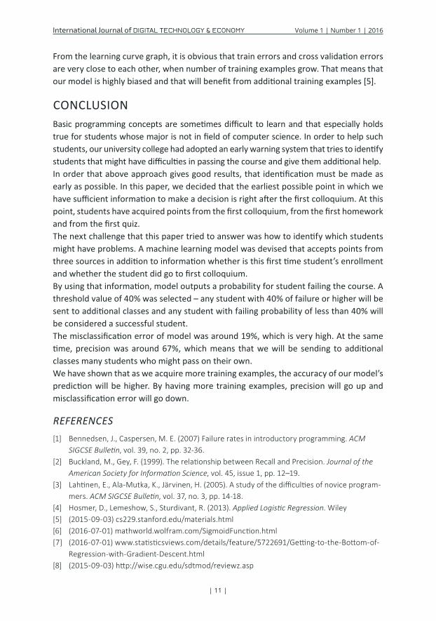
FUTURE PROSPECTSIn this part of the paper, we will try to predict whether the performance of our model will be better when we have more training examples. In order to learn that, we will be drawing a learning curve graph [5], shown in Figure 2.
11070 905020 1006030 804010
5
4.5
4
3.5
3
2.5
2
1.5
1
0.5
0
Numbers of training examples
Train error Cross validation error
Erro
rs
Figure 2: Learning curve graph.
International Journal of DIGITAL TECHNOLOGY & ECONOMY Volume 1 | Number 1 | 2016
| 11 |
From the learning curve graph, it is obvious that train errors and cross validation errors are very close to each other, when number of training examples grow. That means that our model is highly biased and that will benefit from additional training examples [5].
CONCLUSIONBasic programming concepts are sometimes difficult to learn and that especially holds true for students whose major is not in field of computer science. In order to help such students, our university college had adopted an early warning system that tries to identify students that might have difficulties in passing the course and give them additional help. In order that above approach gives good results, that identification must be made as early as possible. In this paper, we decided that the earliest possible point in which we have sufficient information to make a decision is right after the first colloquium. At this point, students have acquired points from the first colloquium, from the first homework and from the first quiz.The next challenge that this paper tried to answer was how to identify which students might have problems. A machine learning model was devised that accepts points from three sources in addition to information whether is this first time student’s enrollment and whether the student did go to first colloquium.By using that information, model outputs a probability for student failing the course. A threshold value of 40% was selected – any student with 40% of failure or higher will be sent to additional classes and any student with failing probability of less than 40% will be considered a successful student.The misclassification error of model was around 19%, which is very high. At the same time, precision was around 67%, which means that we will be sending to additional classes many students who might pass on their own. We have shown that as we acquire more training examples, the accuracy of our model’s prediction will be higher. By having more training examples, precision will go up and misclassification error will go down.
REFERENCES[1] Bennedsen, J., Caspersen, M. E. (2007) Failure rates in introductory programming. ACM
SIGCSE Bulletin, vol. 39, no. 2, pp. 32-36.[2] Buckland,M.,Gey,F.(1999).TherelationshipbetweenRecallandPrecision.Journal of the
American Society for Information Science, vol. 45, issue 1, pp. 12–19.[3] Lahtinen,E.,Ala-Mutka,K.,Järvinen,H.(2005).Astudyofthedifficultiesofnoviceprogram-