EIT Spectroscopy in Hollow Core Fibers Masterthesis Josephine Gutekunst 15. December 2016 5. Physikalisches Institut Examiner: Prof. Dr. Tilman Pfau Second Examiner: Prof. Dr. Martin Dressel
Transcript
EIT Spectroscopy in Hollow Core Fibers
Masterthesis
Josephine Gutekunst
15. December 2016
5. Physikalisches Institut
Examiner: Prof. Dr. Tilman Pfau
Second Examiner: Prof. Dr. Martin Dressel
Ehrenwortliche Erklarung
Ich versichere hiermit ehrenwortlich mit meiner Unterschrift, dass
• ich die Arbeit selbstandig verfasst habe,
• ich keine anderen als die angegebenen Quellen benutzt habe und alle wortlich oder sinn-
gemaß aus anderen Werken ubernommenen Aussagen als solche gekennzeichnet habe,
• die eingereichte Arbeit weder vollstandig noch in wesentlichen Teilen Gegenstand eines
anderen Prufungsverfahrens gewesen ist,
• ich die Arbeit weder vollstandig noch in Teilen bereits veroffentlicht habe,
• der Inhalt des elektronischen Exemplars mit dem des Druckexemplars ubereinstimmt.
Declaration of Authorship
I herby garanty with my signiture, that
• I wrote this thesis on my own,
• I did not use any other sources than those reffered to and that I marked all literal and analo-
gous statements,
• this thesis is neither whole nor partly part of a different examination
• the content of the electronic and the printed exemplar coincide.
Josephine Gutekunst
Stuttgart, 15.12.2016
Summary
In this thesis absorption spectroscopy of a thermal atomic vapor inside hollow core optical fibers is
studied. Two different types of hollow core fiber samples are examined for diffusion behavior and
sub-doppler and EIT spectroscopy. The first sample consists of a capillary of an inner-diameter of
56 µm, with conventional optical fibers spliced on each end. It was shown that this fiber can be
filled with rubidium gas and that the transmission efficiency is suitable for absorption spectroscopy
measurements. Sub-doppler spectroscopy was also examined. The second sample consists of a
conventional vapor cell with two different fiber types mounted inside, a capillary and a kagome
style photonic crystal fiber. Two of these samples were prepared, one with fibers of inner-diameter
of 60 µm and the other one with fibers of an inner-diameter of 20 µm. The diffusion in and out
of these fibers were analyzed to study the effects of LIAD measurements and a theoretical model
to explain the behavior was constructed. The results were compared to previous results for fibers
in a conventional vacuum chamber. Additionally EIT measurements haven been performed for
both core sizes, to evaluated possible applications such as quantum nonlinear optics or the study
of optical bistabilities inside the hollow core of an optical fiber.
Zusammenfassung
In dieser Arbeit wurden Absorptionspektroskopie von thermischem Dampf in einer Hohlkernfaser
durchgefuhrt. Dazu wurden zwei unterschiedliche Arten von Proben mit Hohlkernfasern in Bezug
auf Diffusion, Sub-Doppler-Spektroskopie und EIT untersucht. Die erste Probe bestand aus einer
Kapillare mit einem Innendurchmesser von 56 µm, die an jedem Ende mit einer Glasfaser ver-
bunden war. Es wurde gezeigt, dass diese Hohlkernfaser mit Rubidium gefullt werden konnte
und dass die Transmissionseffizienz geeignet war um Spektroskopiemessungen durchzufuhren.
Außerdem wurden mit ihr Sub-Doppler-Spektroskopiemessungen durchgefuhrt. Die zweite Probe
bestand aus einer herkommlichen Dampfzelle, in der zwei unterschiedliche Hohlkernfasern be-
festigt waren, das eine war eine Kapillare und das andere eine Kagome Kristallfaser. Von dieser
Probenart wurden zwei Stuck gefertigt, in der einen befanden sich Hohlkernfasern mit einem In-
nendurchmesser von 60 µm und in der anderen mit 20 µm. Die Fasern mit den unterschiedlichen
Durchmessern wurden durch LIAD Messungen auf ihr Diffusionsverhalten untersucht und ein the-
oretisches Modell aufgestellt um diese zu erklaren. Die Ergebnisse wurden mit fruheren Ergebnis-
sen von Fasern in einer herkommlichen Vakuumapparatur, verglichen. Schließlich wurden noch
EIT Messungen in allen Fasern durchgefuhrt um mogliche Anwendungen zu untersuchen, wie
zum Beispiel nichtlineare Quantenoptik oder die Untersuchung optischer Bistabilitaten innerhalb
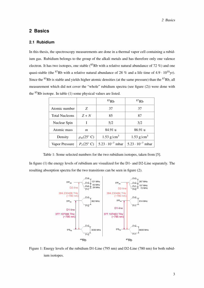
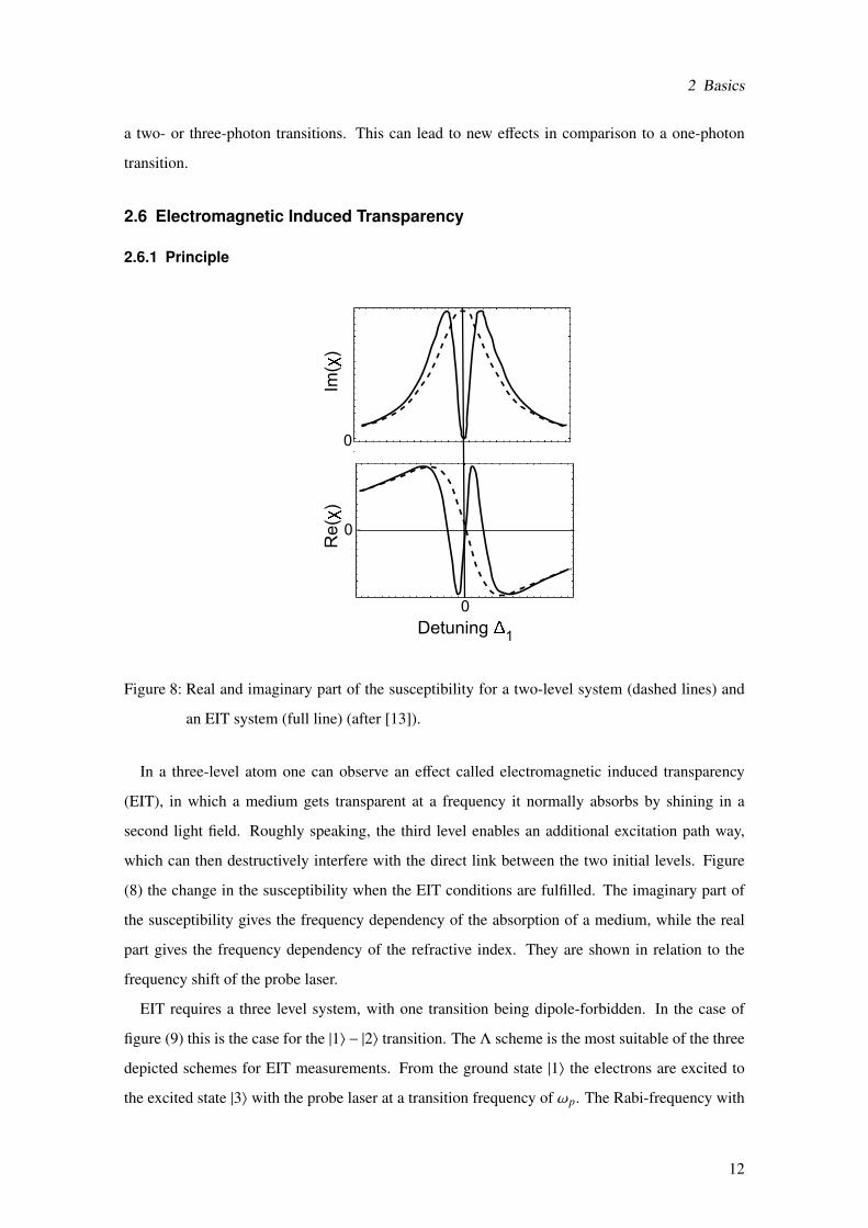
∆1. Remarkably the eigenstate |a0〉 has no contribution from
state |3〉 and is therefore called dark state. If the system is in this state, it is not possible to be
exited into |3〉. This dark state is only stable for the Λ-scheme, which is why it is the only scheme
which shows EIT in the strict sense. The dark state can be addressed with the condition Ωp << Ωc
since then sin(θ) = 0 and the ground state becomes identical to the dark state.
2.6.2 Bistability
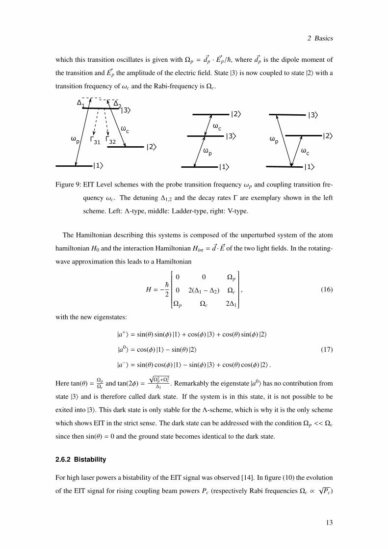
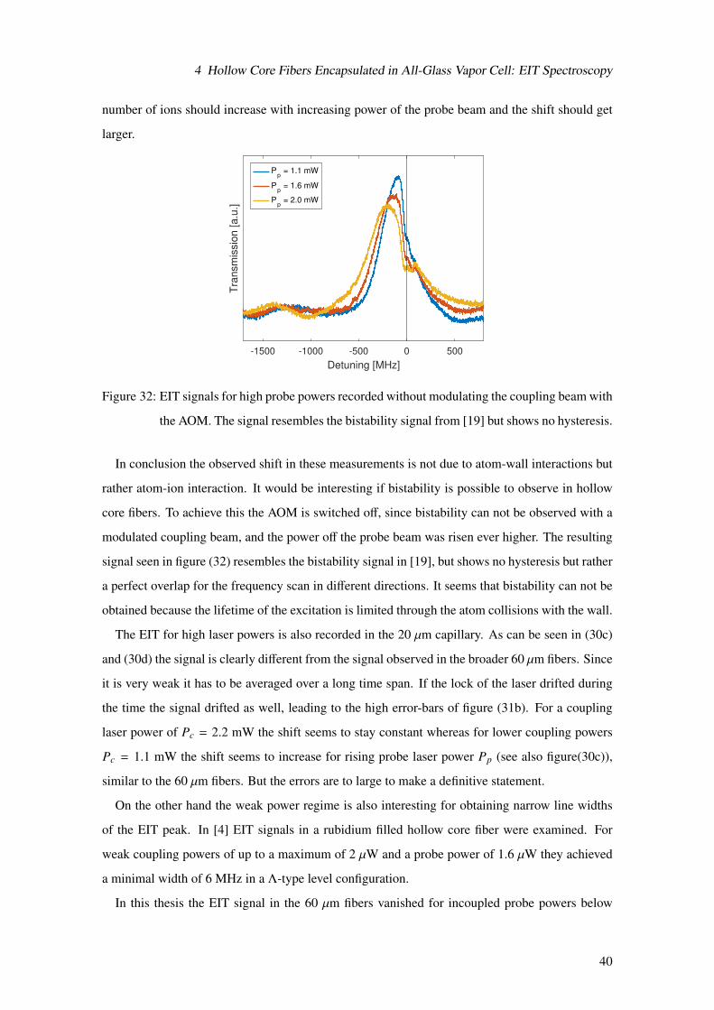
For high laser powers a bistability of the EIT signal was observed [14]. In figure (10) the evolution
of the EIT signal for rising coupling beam powers Pc (respectively Rabi frequencies Ωc ∝√
Pc)
13
2 Basics
can be seen. At first the signal only shows a shift which direction is depending on the polariz-
ability, in figure (10) it is depicted as a red-shift. For higher laser powers however a hysteresis
emerges dependent in which direction the frequency of the coupling laser is tuned. First measure-
Coupling detuning c
Pro
be
tra
nsm
issio
n
0
increase Ωc
Figure 10: Bistability signal as it is observed for example in [14]. For rising coupling laser powers
the signal first gets shifted and for even higher laser powers it shows a hysteresis signal.
This is contributed to ions produced by collision ionization.
ments contributed this effect to dipole-dipole interactions of the Rydberg atoms [15], but present
measurements [14] imply that rather interactions with ions are the cause. The hysteresis results
from the competition of a non-linear energy shift due to the interaction and the decay rate from
the Rydberg state. The energy shift is dependent on the Rydberg population. When the laser is
scanned from the blue detuned side to the red the Rydberg population is build up and it sustains
the ability to excite additional atoms even away from resonance. At a certain point the detuning
however gets to large and the decay mechanism dominates. This can be seen in a sudden break-
down in the probe transmission in figure (10). When the laser is scanned from the red detuned to
the blue detuned though the Rydberg population stays low in the bistable region until the detuning
becomes small enough to excite the atoms.
14
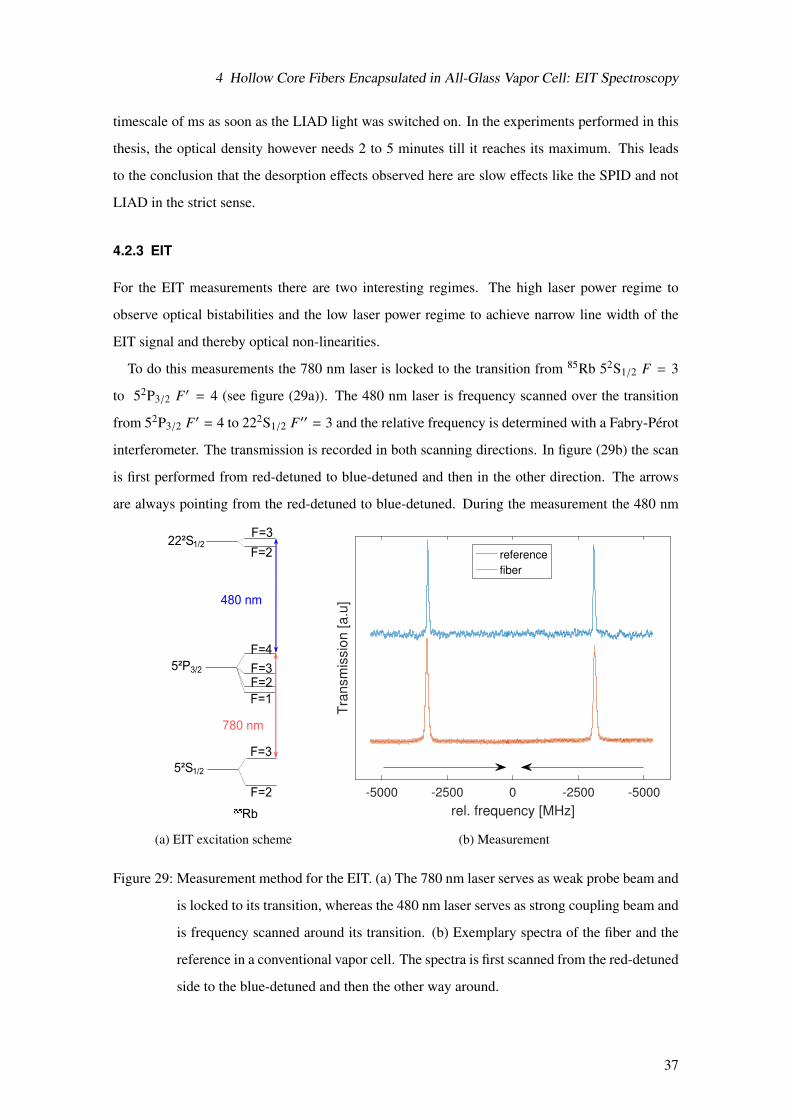
3 Fiber Series: Spectroscopy Below the Doppler Limit
3 Fiber Series: Spectroscopy Below the Doppler Limit
3.1 Setup
3.1.1 Cell
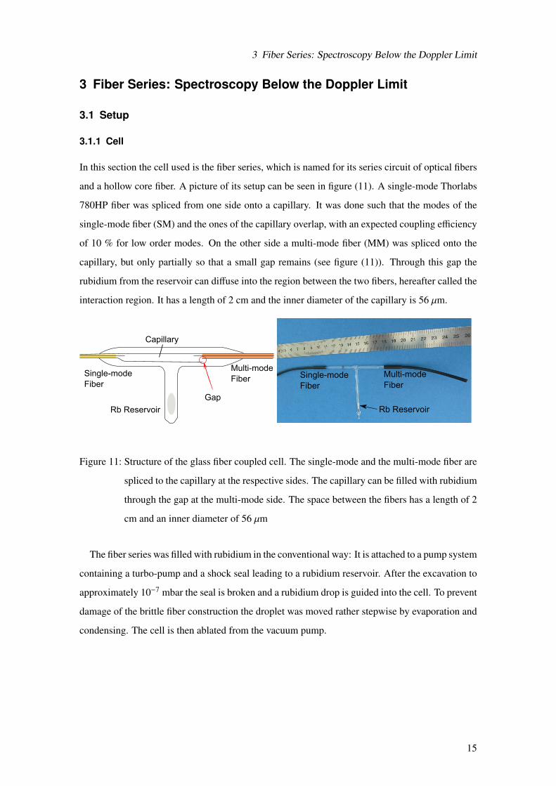
In this section the cell used is the fiber series, which is named for its series circuit of optical fibers
and a hollow core fiber. A picture of its setup can be seen in figure (11). A single-mode Thorlabs
780HP fiber was spliced from one side onto a capillary. It was done such that the modes of the
single-mode fiber (SM) and the ones of the capillary overlap, with an expected coupling efficiency
of 10 % for low order modes. On the other side a multi-mode fiber (MM) was spliced onto the
capillary, but only partially so that a small gap remains (see figure (11)). Through this gap the
rubidium from the reservoir can diffuse into the region between the two fibers, hereafter called the
interaction region. It has a length of 2 cm and the inner diameter of the capillary is 56 µm.
Single-mode
Fiber
Multi-mode
Fiber
Rb Reservoir
Gap
Capillary
Rb Reservoir
Single-mode
Fiber
Multi-mode
Fiber
Figure 11: Structure of the glass fiber coupled cell. The single-mode and the multi-mode fiber are
spliced to the capillary at the respective sides. The capillary can be filled with rubidium
through the gap at the multi-mode side. The space between the fibers has a length of 2
cm and an inner diameter of 56 µm
The fiber series was filled with rubidium in the conventional way: It is attached to a pump system
containing a turbo-pump and a shock seal leading to a rubidium reservoir. After the excavation to
approximately 10−7 mbar the seal is broken and a rubidium drop is guided into the cell. To prevent
damage of the brittle fiber construction the droplet was moved rather stepwise by evaporation and
condensing. The cell is then ablated from the vacuum pump.
15
3 Fiber Series: Spectroscopy Below the Doppler Limit
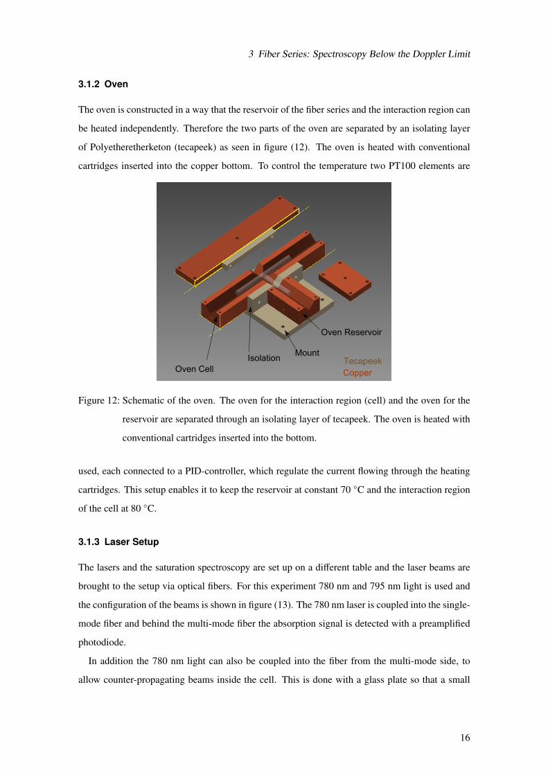
3.1.2 Oven
The oven is constructed in a way that the reservoir of the fiber series and the interaction region can
be heated independently. Therefore the two parts of the oven are separated by an isolating layer
of Polyetheretherketon (tecapeek) as seen in figure (12). The oven is heated with conventional
cartridges inserted into the copper bottom. To control the temperature two PT100 elements are
CopperOven Cell
Oven Reservoir
MountIsolation Tecapeek
Figure 12: Schematic of the oven. The oven for the interaction region (cell) and the oven for the
reservoir are separated through an isolating layer of tecapeek. The oven is heated with
conventional cartridges inserted into the bottom.
used, each connected to a PID-controller, which regulate the current flowing through the heating
cartridges. This setup enables it to keep the reservoir at constant 70 C and the interaction region
of the cell at 80 C.
3.1.3 Laser Setup
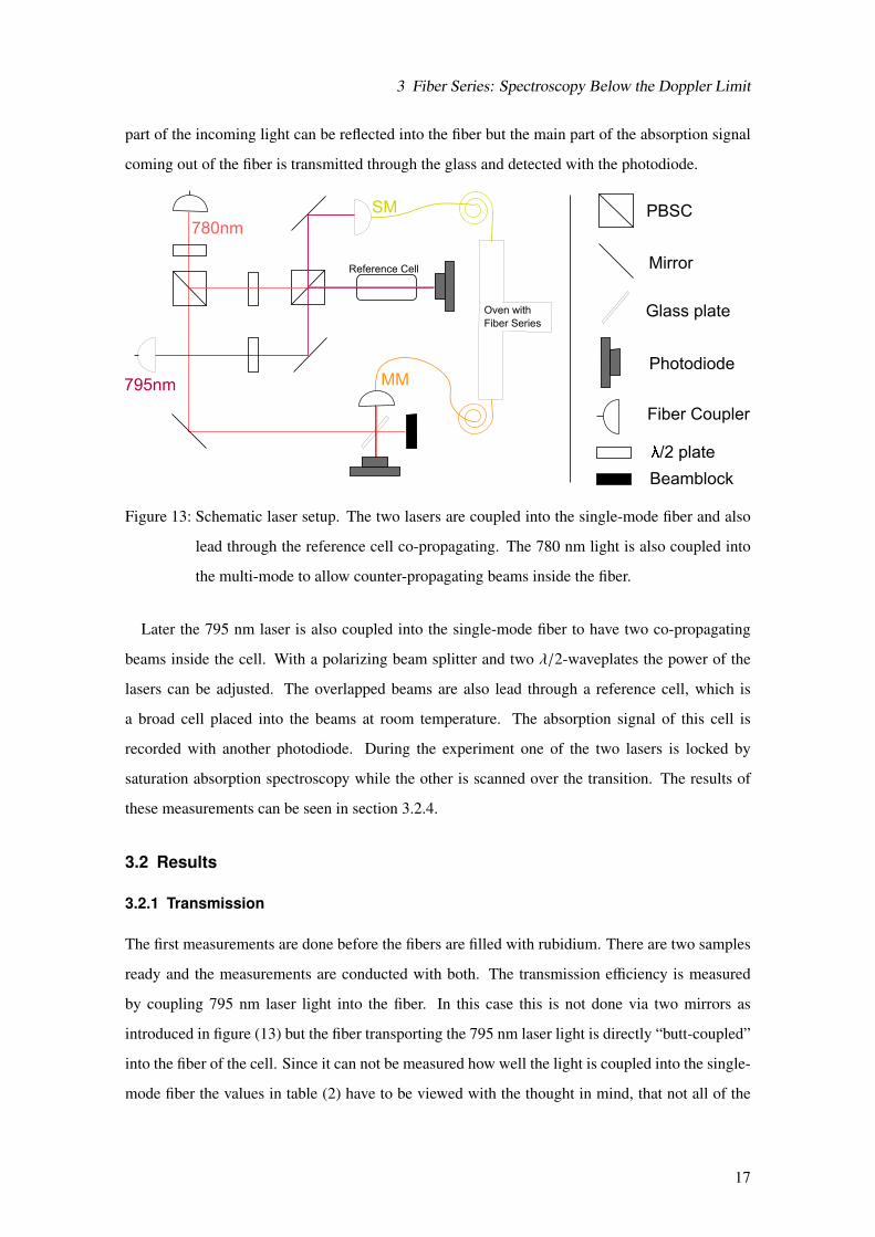
The lasers and the saturation spectroscopy are set up on a different table and the laser beams are
brought to the setup via optical fibers. For this experiment 780 nm and 795 nm light is used and
the configuration of the beams is shown in figure (13). The 780 nm laser is coupled into the single-
mode fiber and behind the multi-mode fiber the absorption signal is detected with a preamplified
photodiode.
In addition the 780 nm light can also be coupled into the fiber from the multi-mode side, to
allow counter-propagating beams inside the cell. This is done with a glass plate so that a small
16
3 Fiber Series: Spectroscopy Below the Doppler Limit
part of the incoming light can be reflected into the fiber but the main part of the absorption signal
coming out of the fiber is transmitted through the glass and detected with the photodiode.
795nm
780nm
MM
SM
Oven with
Fiber Series
PBSC
Mirror
Photodiode
/2 plate
Beamblock
Glass plate
Fiber Coupler
Reference Cell
Figure 13: Schematic laser setup. The two lasers are coupled into the single-mode fiber and also
lead through the reference cell co-propagating. The 780 nm light is also coupled into
the multi-mode to allow counter-propagating beams inside the fiber.
Later the 795 nm laser is also coupled into the single-mode fiber to have two co-propagating
beams inside the cell. With a polarizing beam splitter and two λ/2-waveplates the power of the
lasers can be adjusted. The overlapped beams are also lead through a reference cell, which is
a broad cell placed into the beams at room temperature. The absorption signal of this cell is
recorded with another photodiode. During the experiment one of the two lasers is locked by
saturation absorption spectroscopy while the other is scanned over the transition. The results of
these measurements can be seen in section 3.2.4.
3.2 Results
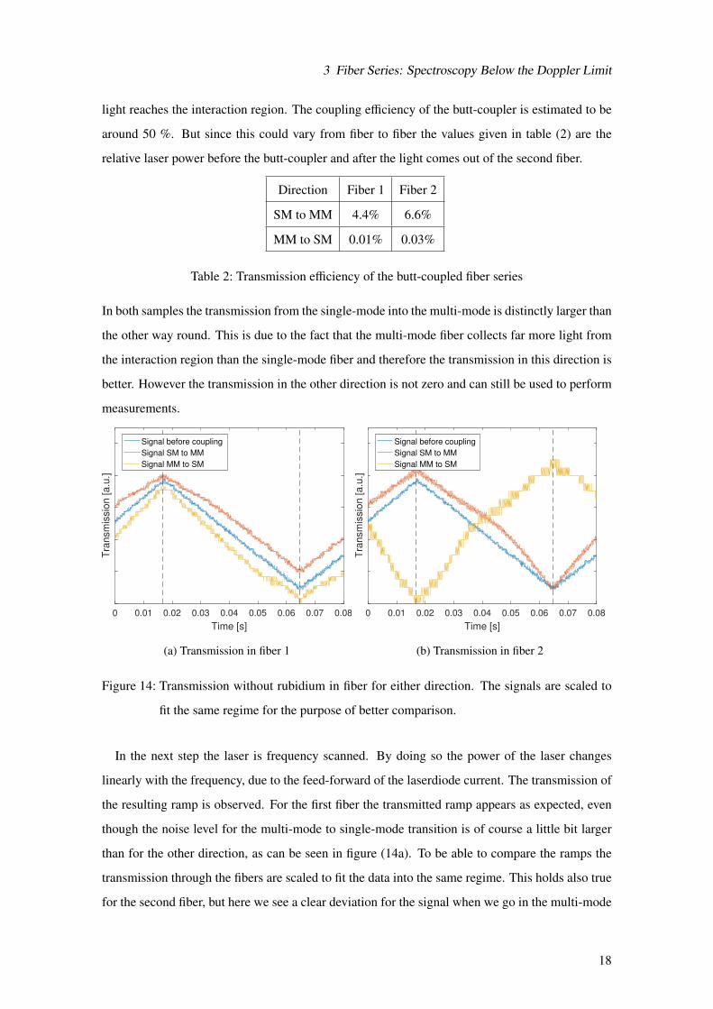
3.2.1 Transmission
The first measurements are done before the fibers are filled with rubidium. There are two samples
ready and the measurements are conducted with both. The transmission efficiency is measured
by coupling 795 nm laser light into the fiber. In this case this is not done via two mirrors as
introduced in figure (13) but the fiber transporting the 795 nm laser light is directly “butt-coupled”
into the fiber of the cell. Since it can not be measured how well the light is coupled into the single-
mode fiber the values in table (2) have to be viewed with the thought in mind, that not all of the
17
3 Fiber Series: Spectroscopy Below the Doppler Limit
light reaches the interaction region. The coupling efficiency of the butt-coupler is estimated to be
around 50 %. But since this could vary from fiber to fiber the values given in table (2) are the
relative laser power before the butt-coupler and after the light comes out of the second fiber.
Direction Fiber 1 Fiber 2
SM to MM 4.4% 6.6%
MM to SM 0.01% 0.03%
Table 2: Transmission efficiency of the butt-coupled fiber series
In both samples the transmission from the single-mode into the multi-mode is distinctly larger than
the other way round. This is due to the fact that the multi-mode fiber collects far more light from
the interaction region than the single-mode fiber and therefore the transmission in this direction is
better. However the transmission in the other direction is not zero and can still be used to perform
measurements.
0 0.01 0.02 0.03 0.04 0.05 0.06 0.07 0.08
Time [s]
Tra
nsm
issio
n [
a.u
.]
Signal before coupling
Signal SM to MM
Signal MM to SM
(a) Transmission in fiber 1
0 0.01 0.02 0.03 0.04 0.05 0.06 0.07 0.08
Time [s]
Tra
nsm
issio
n [
a.u
.]
Signal before coupling
Signal SM to MM
Signal MM to SM
(b) Transmission in fiber 2
Figure 14: Transmission without rubidium in fiber for either direction. The signals are scaled to
fit the same regime for the purpose of better comparison.
In the next step the laser is frequency scanned. By doing so the power of the laser changes
linearly with the frequency, due to the feed-forward of the laserdiode current. The transmission of
the resulting ramp is observed. For the first fiber the transmitted ramp appears as expected, even
though the noise level for the multi-mode to single-mode transition is of course a little bit larger
than for the other direction, as can be seen in figure (14a). To be able to compare the ramps the
transmission through the fibers are scaled to fit the data into the same regime. This holds also true
for the second fiber, but here we see a clear deviation for the signal when we go in the multi-mode
18
3 Fiber Series: Spectroscopy Below the Doppler Limit
to single-mode direction, and with small nudges on the fiber the signal fluctuates strongly.
Fiber 1 is the first one to be filled with rubidium. Unfortunately the fibers broke, most likely
during the filling or the transport of the fiber. In both, the single-mode and the multi-mode fiber,
one could see a rupture under the microscope and the transmission efficiency in the direction
single-mode to multi-mode dropped to 0.05%. Therefore all the following measurements are done
with the second sample.
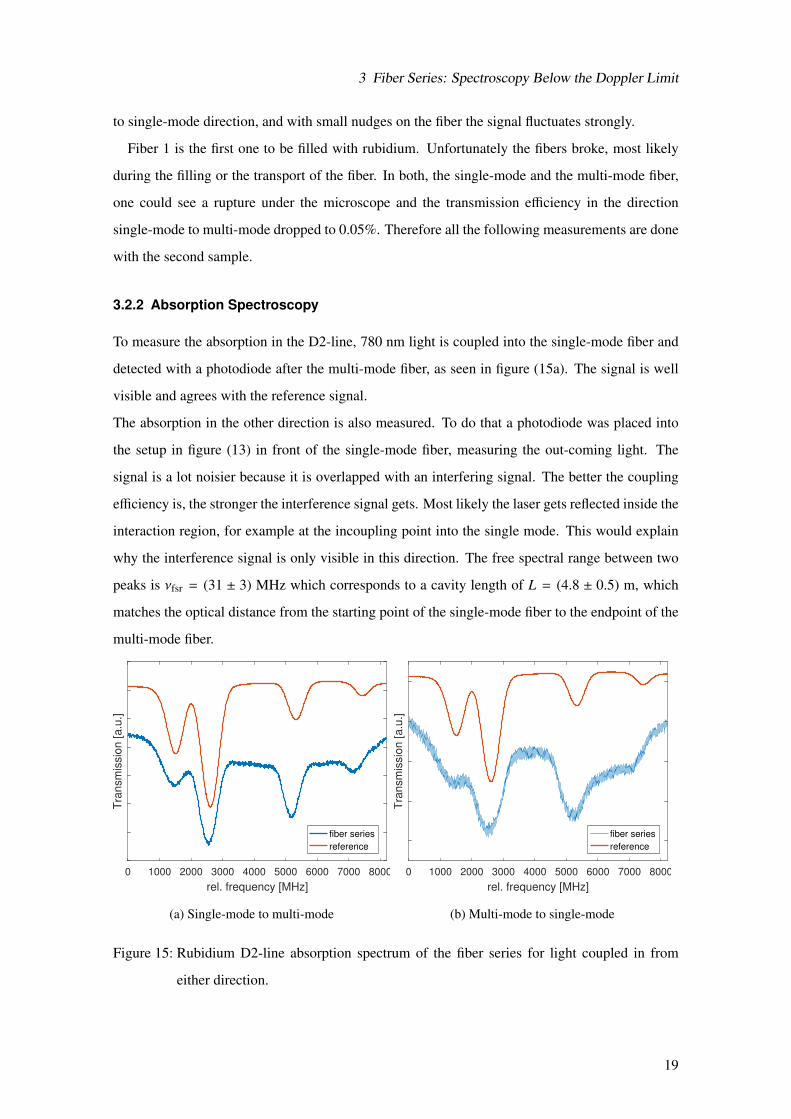
3.2.2 Absorption Spectroscopy
To measure the absorption in the D2-line, 780 nm light is coupled into the single-mode fiber and
detected with a photodiode after the multi-mode fiber, as seen in figure (15a). The signal is well
visible and agrees with the reference signal.
The absorption in the other direction is also measured. To do that a photodiode was placed into
the setup in figure (13) in front of the single-mode fiber, measuring the out-coming light. The
signal is a lot noisier because it is overlapped with an interfering signal. The better the coupling
efficiency is, the stronger the interference signal gets. Most likely the laser gets reflected inside the
interaction region, for example at the incoupling point into the single mode. This would explain
why the interference signal is only visible in this direction. The free spectral range between two
peaks is νfsr = (31 ± 3) MHz which corresponds to a cavity length of L = (4.8 ± 0.5) m, which
matches the optical distance from the starting point of the single-mode fiber to the endpoint of the
multi-mode fiber.
0 1000 2000 3000 4000 5000 6000 7000 8000
rel. frequency [MHz]
Tra
nsm
issio
n [a.u
.]
fiber series
reference
(a) Single-mode to multi-mode
0 1000 2000 3000 4000 5000 6000 7000 8000
rel. frequency [MHz]
Tra
nsm
issio
n [a.u
.]
fiber series
reference
(b) Multi-mode to single-mode
Figure 15: Rubidium D2-line absorption spectrum of the fiber series for light coupled in from
either direction.
19
3 Fiber Series: Spectroscopy Below the Doppler Limit
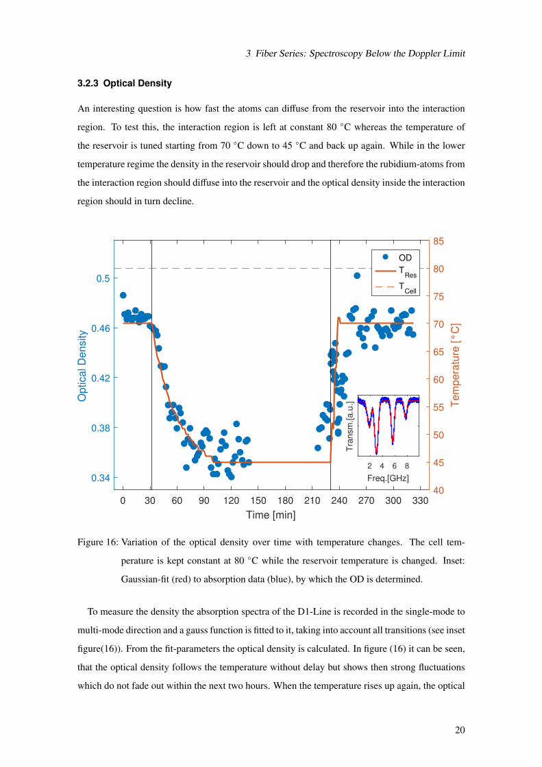
3.2.3 Optical Density
An interesting question is how fast the atoms can diffuse from the reservoir into the interaction
region. To test this, the interaction region is left at constant 80 C whereas the temperature of
the reservoir is tuned starting from 70 C down to 45 C and back up again. While in the lower
temperature regime the density in the reservoir should drop and therefore the rubidium-atoms from
the interaction region should diffuse into the reservoir and the optical density inside the interaction
region should in turn decline.
0 30 60 90 120 150 180 210 240 270 300 330
Time [min]
0.34
0.38
0.42
0.46
0.5
Optical D
ensity
40
45
50
55
60
65
70
75
80
85
Tem
pera
ture
[°
C]
OD
TRes
TCell
2 4 6 8
Freq.[GHz]
Tra
nsm
.[a
.u.]
Figure 16: Variation of the optical density over time with temperature changes. The cell tem-
perature is kept constant at 80 C while the reservoir temperature is changed. Inset:
Gaussian-fit (red) to absorption data (blue), by which the OD is determined.
To measure the density the absorption spectra of the D1-Line is recorded in the single-mode to
multi-mode direction and a gauss function is fitted to it, taking into account all transitions (see inset
figure(16)). From the fit-parameters the optical density is calculated. In figure (16) it can be seen,
that the optical density follows the temperature without delay but shows then strong fluctuations
which do not fade out within the next two hours. When the temperature rises up again, the optical
20
3 Fiber Series: Spectroscopy Below the Doppler Limit
density follows again nearly instantaneous and reaches a density a bit smaller and with stronger
fluctuations than before. Again, it will take several hours until the system equilibrates.
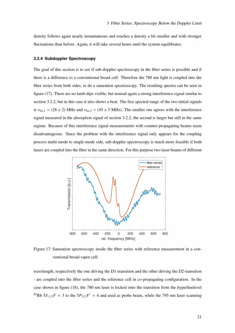
3.2.4 Subdoppler Spectroscopy
The goal of this section is to see if sub-doppler spectroscopy in the fiber series is possible and if
there is a difference to a conventional broad cell. Therefore the 780 nm light is coupled into the
fiber series from both sides, to do a saturation spectroscopy. The resulting spectra can be seen in
figure (17). There are no lamb dips visible, but instead again a strong interference signal similar to
section 3.2.2, but in this case it also shows a beat. The free spectral range of the two initial signals
is νfsr,1 = (28 ± 2) MHz and νfsr,2 = (45 ± 5 MHz). The smaller one agrees with the interference
signal measured in the absorption signal of section 3.2.2, the second is larger but still in the same
regime. Because of this interference signal measurements with counter-propagating beams seem
disadvantageous. Since the problem with the interference signal only appears for the coupling
process multi-mode to single-mode side, sub-doppler spectroscopy is much more feasible if both
lasers are coupled into the fiber in the same direction. For this purpose two laser beams of different
-800 -600 -400 -200 0 200 400 600 800
rel. frequency [MHz]
Tra
nsm
issio
n [
a.u
.]
fiber series
reference
Figure 17: Saturation spectroscopy inside the fiber series with reference measurement in a con-
ventional broad vapor cell.
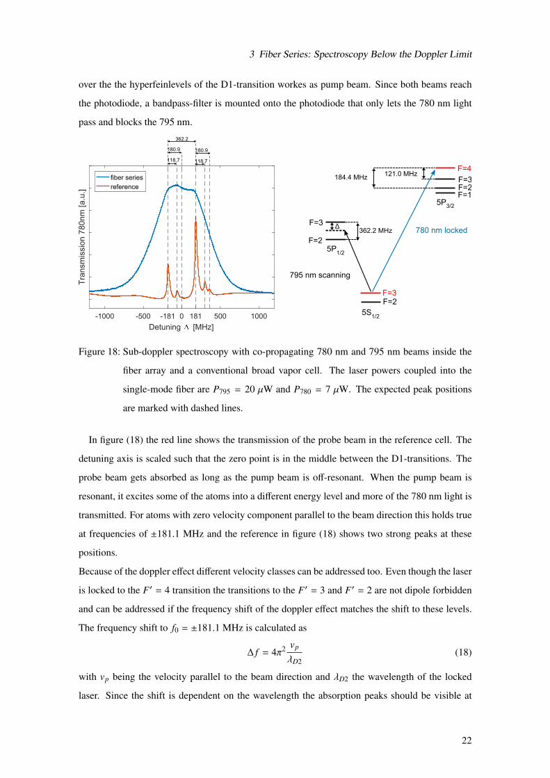
wavelength, respectively the one driving the D1-transition and the other driving the D2-transition
- are coupled into the fiber series and the reference cell in co-propagating configuration. In the
case shown in figure (18), the 780 nm laser is locked onto the transition from the hyperfinelevel85Rb 5S 1/2F = 3 to the 5P3/2F′ = 4 and used as probe beam, while the 795 nm laser scanning
21
3 Fiber Series: Spectroscopy Below the Doppler Limit
over the the hyperfeinlevels of the D1-transition workes as pump beam. Since both beams reach
the photodiode, a bandpass-filter is mounted onto the photodiode that only lets the 780 nm light
pass and blocks the 795 nm.
-1000 -500 -181 0 181 500 1000
Detuning [MHz]
Tra
nsm
issio
n 7
80nm
[a.u
.]
fiber series
reference
118.7
180.9
118.7
180.9
362.2
F=2
F=2
F=3
F=2
F=3
F=3
F=4
F=1
5S1/2
5P1/2
5P3/2
780 nm locked
795 nm scanning
362.2 MHz
121.0 MHz184.4 MHz
Δ
Figure 18: Sub-doppler spectroscopy with co-propagating 780 nm and 795 nm beams inside the
fiber array and a conventional broad vapor cell. The laser powers coupled into the
single-mode fiber are P795 = 20 µW and P780 = 7 µW. The expected peak positions
are marked with dashed lines.
In figure (18) the red line shows the transmission of the probe beam in the reference cell. The
detuning axis is scaled such that the zero point is in the middle between the D1-transitions. The
probe beam gets absorbed as long as the pump beam is off-resonant. When the pump beam is
resonant, it excites some of the atoms into a different energy level and more of the 780 nm light is
transmitted. For atoms with zero velocity component parallel to the beam direction this holds true
at frequencies of ±181.1 MHz and the reference in figure (18) shows two strong peaks at these
positions.
Because of the doppler effect different velocity classes can be addressed too. Even though the laser
is locked to the F′ = 4 transition the transitions to the F′ = 3 and F′ = 2 are not dipole forbidden
and can be addressed if the frequency shift of the doppler effect matches the shift to these levels.
The frequency shift to f0 = ±181.1 MHz is calculated as
∆ f = 4π2 vp
λD2(18)
with vp being the velocity parallel to the beam direction and λD2 the wavelength of the locked
laser. Since the shift is dependent on the wavelength the absorption peaks should be visible at
22
3 Fiber Series: Spectroscopy Below the Doppler Limit
frequency shifts of
∆ fD1 = ∆ fλD2
λD1(19)
which correspond to ∆ fD1 = 118.7 MHz for the F′ = 3 transition and ∆ fD1 = 180.9 MHz for
the F′ = 2 transition. In figure (18) these positions are marked with dashed lines and they fit the
position of the peaks in the reference very well.
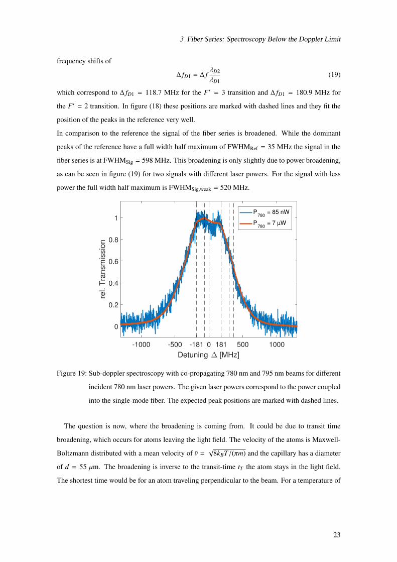
In comparison to the reference the signal of the fiber series is broadened. While the dominant
peaks of the reference have a full width half maximum of FWHMRef = 35 MHz the signal in the
fiber series is at FWHMSig = 598 MHz. This broadening is only slightly due to power broadening,
as can be seen in figure (19) for two signals with different laser powers. For the signal with less
power the full width half maximum is FWHMSig,weak = 520 MHz.
-1000 -500 -181 0 181 500 1000
Detuning ∆ [MHz]
0
0.2
0.4
0.6
0.8
1
rel. T
ran
sm
issio
n
P780
= 85 nW
P780
= 7 µW
Figure 19: Sub-doppler spectroscopy with co-propagating 780 nm and 795 nm beams for different
incident 780 nm laser powers. The given laser powers correspond to the power coupled
into the single-mode fiber. The expected peak positions are marked with dashed lines.
The question is now, where the broadening is coming from. It could be due to transit time
broadening, which occurs for atoms leaving the light field. The velocity of the atoms is Maxwell-
Boltzmann distributed with a mean velocity of v =√
8kBT/(πm) and the capillary has a diameter
of d = 55 µm. The broadening is inverse to the transit-time tT the atom stays in the light field.
The shortest time would be for an atom traveling perpendicular to the beam. For a temperature of
23
3 Fiber Series: Spectroscopy Below the Doppler Limit
80 C the transit-time broadening in this system should be
∆ FWHMtrans =1tT
=vd≈ 2π · 0.86 MHz, (20)
which is very small and does not explain a broadening of a few 100 MHz.
Another reason could be pressure broadening through contamination with other gases. If the
fiber series has a small leak air could diffuse into it. Air consists to 78% of N2. The power
broadening of the D2 line due to N2 is given in [16] as 18.3± 0.2 MHz/Torr. The weak signal was
broadened by 485 MHz, for this to be caused by pressure broadening with N2 the pressure inside
the fiber series has to be at 35.2 ± 0.4 mbar. This is pretty high but could be true if the fiber really
has a leak somewhere.
24
4 Hollow Core Fibers Encapsulated in All-Glass Vapor Cell: EIT Spectroscopy
4 Hollow Core Fibers Encapsulated in All-Glass Vapor Cell: EIT
Spectroscopy
4.1 Setup
4.1.1 Cell
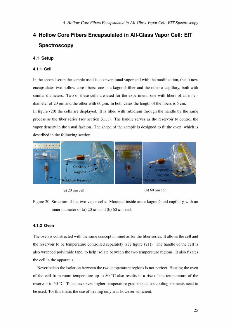
In the second setup the sample used is a conventional vapor cell with the modification, that it now
encapsulates two hollow core fibers: one is a kagome fiber and the other a capillary, both with
similar diameters. Two of these cells are used for the experiment, one with fibers of an inner-
diameter of 20 µm and the other with 60 µm. In both cases the length of the fibers is 5 cm.
In figure (20) the cells are displayed. It is filled with rubidium through the handle by the same
process as the fiber series (see section 3.1.1). The handle serves as the reservoir to control the
vapor density in the usual fashion. The shape of the sample is designed to fit the oven, which is
described in the following section.
Rubidium Reservoir
Kagome
Capillary
(a) 20 µm cell
Rubidium Reservoir
Kagome
Capillary
(b) 60 µm cell
Figure 20: Structure of the two vapor cells. Mounted inside are a kagome and capillary with an
inner diameter of (a) 20 µm and (b) 60 µm each.
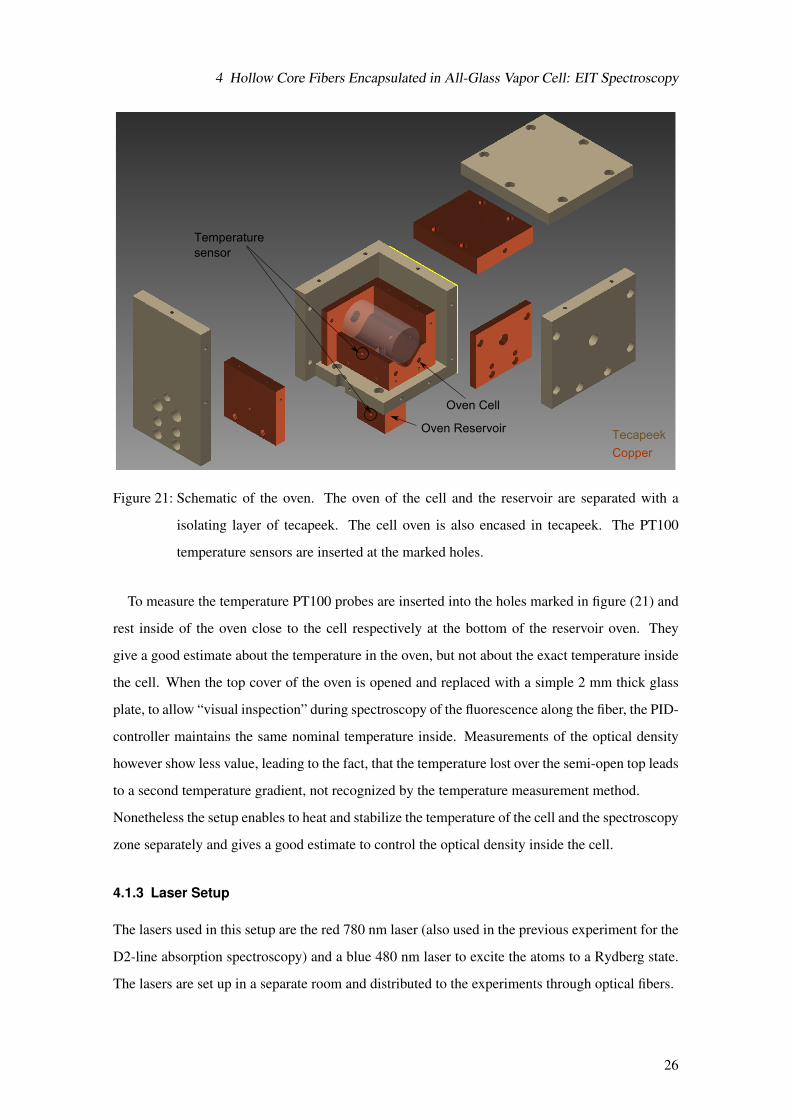
4.1.2 Oven
The oven is constructed with the same concept in mind as for the fiber series. It allows the cell and
the reservoir to be temperature controlled separately (see figure (21)). The handle of the cell is
also wrapped polyimide tape, to help isolate between the two temperature regions. It also fixates
the cell in the apparatus.
Nevertheless the isolation between the two temperature regions is not perfect. Heating the oven
of the cell from room temperature up to 80 C also results in a rise of the temperature of the
reservoir to 50 C. To achieve even higher temperature gradients active cooling elements need to
be used. Tor this thesis the use of heating only was however sufficient.
25
4 Hollow Core Fibers Encapsulated in All-Glass Vapor Cell: EIT Spectroscopy
Tecapeek
Copper
Oven Reservoir
Oven Cell
Temperature
sensor
Figure 21: Schematic of the oven. The oven of the cell and the reservoir are separated with a
isolating layer of tecapeek. The cell oven is also encased in tecapeek. The PT100
temperature sensors are inserted at the marked holes.
To measure the temperature PT100 probes are inserted into the holes marked in figure (21) and
rest inside of the oven close to the cell respectively at the bottom of the reservoir oven. They
give a good estimate about the temperature in the oven, but not about the exact temperature inside
the cell. When the top cover of the oven is opened and replaced with a simple 2 mm thick glass
plate, to allow “visual inspection” during spectroscopy of the fluorescence along the fiber, the PID-
controller maintains the same nominal temperature inside. Measurements of the optical density
however show less value, leading to the fact, that the temperature lost over the semi-open top leads
to a second temperature gradient, not recognized by the temperature measurement method.
Nonetheless the setup enables to heat and stabilize the temperature of the cell and the spectroscopy
zone separately and gives a good estimate to control the optical density inside the cell.
4.1.3 Laser Setup
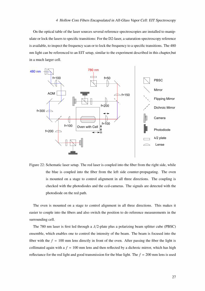
The lasers used in this setup are the red 780 nm laser (also used in the previous experiment for the
D2-line absorption spectroscopy) and a blue 480 nm laser to excite the atoms to a Rydberg state.
The lasers are set up in a separate room and distributed to the experiments through optical fibers.
26
4 Hollow Core Fibers Encapsulated in All-Glass Vapor Cell: EIT Spectroscopy
On the optical table of the laser sources several reference spectroscopies are installed to manip-
ulate or lock the lasers to specific transitions: For the D2-laser, a saturation-spectroscopy reference
is available, to inspect the frequency scan or to lock the frequency to a specific transitions. The 480
nm light can be referenced to an EIT setup, similar to the experiment described in this chapter,but
in a much larger cell.
780 nm480 nm
PBSC
Mirror
Flipping Mirror
Dichroic Mirror
Oven with Cell
Camera
Photodiode
/2 plate
Lense
f=200
f=100
f=100
f=200
f=50
f=150AOM
f=100
f=300
Figure 22: Schematic laser setup. The red laser is coupled into the fiber from the right side, while
the blue is coupled into the fiber from the left side counter-propagating. The oven
is mounted on a stage to control alignment in all three directions. The coupling is
checked with the photodiodes and the ccd-cameras. The signals are detected with the
photodiode on the red path.
The oven is mounted on a stage to control alignment in all three directions. This makes it
easier to couple into the fibers and also switch the position to do reference measurements in the
surrounding cell.
The 780 nm laser is first led through a λ/2-plate plus a polarizing beam splitter cube (PBSC)
ensemble, which enables one to control the intensity of the beam. The beam is focused into the
fiber with the f = 100 mm lens directly in front of the oven. After passing the fiber the light is
collimated again with a f = 100 mm lens and then reflected by a dichroic mirror, which has high
reflectance for the red light and good transmission for the blue light. The f = 200 mm lens is used
27
4 Hollow Core Fibers Encapsulated in All-Glass Vapor Cell: EIT Spectroscopy
to enlarge the image of the end of the fiber and project it onto the ccd-camera. The coupling is
optimized through visual confirmation of the mode form and also of the transmitted power checked
with the photodiode. Later this photodiode is also used to record the absorption spectra as well as
the EIT signal.
The blue 480 nm beam is set up similarly to the red beam but coupled into the fiber counter-
propagating. There are only two differences: Behind the oven, instead of a dichroic mirror a
flipping mirror is used since this part of the beam is only needed for the coupling process.
Additionally, the first f = 100 mm lens is used to focus the beam into an acoustic optical modulator
(AOM). It is set up such that if the AOM is switched on, 80% of the light gets transmitted in the
first mode. Through this method the strength of the blue beam coupled into the fiber can be
modulated and a lock-in-amplifier can be used.
4.2 Results
4.2.1 Optical Density
The characterization of the system in comparison to the conventional system containing a vacuum-
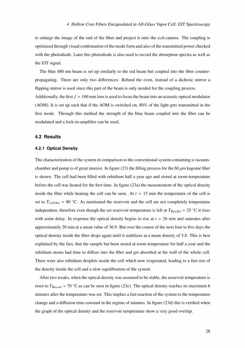
chamber and pump is of great interest. In figure (23) the filling process for the 60 µm kagome fiber
is shown. The cell had been filled with rubidium half a year ago and stored at room-temperature
before the cell was heated for the first time. In figure (23a) the measurement of the optical density
inside the fiber while heating the cell can be seen. At t = 15 min the temperature of the cell is
set to TCell,Set = 80 C. As mentioned the reservoir and the cell are not completely temperature
independent, therefore even though the set reservoir temperature is left at TRes,Set = 25 C it rises
with some delay. In response the optical density begins to rise at t = 26 min and saturates after
approximately 20 min at a mean value of 36.9. But over the course of the next four to five days the
optical density inside the fiber drops again until it stabilizes at a mean density of 5.8. This is best
explained by the fact, that the sample hat been stored at room temperature for half a year and the
rubidium atoms had time to diffuse into the fiber and get absorbed at the wall of the whole cell.
There were also rubidium droplets inside the cell which now evaporated, leading to a fast rise of
the density inside the cell and a slow equilibration of the system.
After two weaks, when the optical density was assumed to be stable, the reservoir temperature is
risen to TRes,set = 70 C as can be seen in figure (23c). The optical density reaches its maximum 6
minutes after the temperature was set. This implies a fast reaction of the system to the temperature
change and a diffusion time constant in the regime of minutes. In figure (23d) this is verified when
the graph of the optical density and the reservoir temperature show a very good overlap.
28
4 Hollow Core Fibers Encapsulated in All-Glass Vapor Cell: EIT Spectroscopy
The optical density stays constant after the last temperature scan. However when the oven top
is lifted and the tecapeek and the thick copper plate do not isolate the oven any longer the optical
density drops even though the temperature measured inside the oven stays constant. This means
there is a temperature gradient inside the oven and the diffusion time constant measured may not
be true since the change of the optical density could be from atoms adsorbing and desorbing of the
fiber wall due to temperature changes of it. Therefore LIAD measurements were done in section
4.2.2 to exclude this possible error.
0 15 30 45 60 75 90 105
Time [min]
0
5
10
15
20
25
30
35
40
Optical D
ensity
20
30
40
50
60
70
80
Tem
pera
ture
[°
C]
OD
TRes
TCell
(a) Heating cell day 0
laser detuning
transm
issio
n
(b) Filling process of [2]
0 15 30 45 60 75
Time [min]
0
5
10
15
20
25
30
35
40
Optical D
ensity
45
50
55
60
65
70
75
80
85
Tem
pera
ture
[°
C]
OD
TRes
TCell
(c) Heating reservoir day 15
0 30 60 90 120 150 180 210 240
Time [min]
0
5
10
15
20
25
30
35
40
Optical D
ensity
45
50
55
60
65
70
75
80
85
Tem
pera
ture
[°
C]
OD
TRes
TCell
(d) Scan TRes day 18
Figure 23: Optical Density inside 60 µm kagome with temperature changes. (a) Heating of the
cell to TCell,set = 80 C leaving TRes,set = 25 C. (c) Setting reservoir temperature to
TRes,set = 70C. (d) Temperature scan TRes,set = 70...50...70 C (b) Filling process of
60 µm wide and 85 mm long kagome fiber in a conventional setup [2]. The temperatures
are at TRes = 45 C and TCell = 80 C.
In comparison to this the filling process from the master thesis of Christian Veit [2] is shown in
29
4 Hollow Core Fibers Encapsulated in All-Glass Vapor Cell: EIT Spectroscopy
figure (23b) (note that the time-scale differs by a factor of 100). In this thesis the setup consists of
a conventional vacuum-chamber with the fibers mounted inside and a cesium reservoir. The fiber
had a length of 85 mm and an inner diameter of 60 µm . At t = 0 the reservoir and the cell are
heated to TRes = 45 C and TCell = 80 C respectively. In the first 10 hours no cesium can be
detected, most likely because of the cesium atoms depositing on the wall surfaces of the vacuum
chamber. But after that delay the optical density rises quickly inside the chamber and the optical
density inside the fiber follows. Noticeable is here, that the time scale of the diffusion process into
the fiber is in the regime of hours whereas in the case of the current thesis process happens within
minutes. To explain this some facts have to be taken into account.
In [2] the fiber is first exposed to cesium at the time t = 10 h and from there a curing process takes
place, where the atoms adsorbe on the surface and then diffuse into the glass bulk of the fiber.
Therefore the atoms indeed diffuse into the fiber but do not contribute to a rise in atomic density
in the fiber core. In the present thesis this curing process could not be observed due to various
reasons. First of all the fiber was first exposed to the rubidium vapor during the filling process
of the cell, when the cell was still connected to the vacuum pump and not in the optical set up.
Secondly when the cell was ablated from the vacuum setup the optical setup was not ready yet
since at that time the setup for the fiber series was installed first. So the fiber had enough time to
go through the curing process.
Nevertheless the fiber cell holds some advantages in comparison to the conventional vacuum-
chamber. Except for the (one time) filling process it gets by without a big vacuum setup. And the
vacuum setup can be used to fill multiple cells with different fiber types with minimal cleaning
effort of the vacuum parts. These cells can then easily be brought into the optical setup. Switching
times between fibers are only limited to the time it takes to open and close the oven and to couple
into the new fiber. If the cells are standardizes in respect to the fiber position inside the cell, the
coupling time can be reduces drastically.
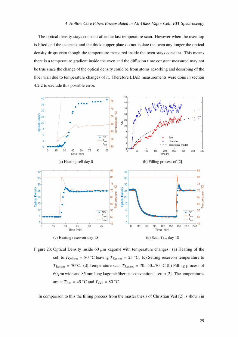
In figure (24) the difference in optical density of the fiber and the surrounding cell is measured
for all 4 different types of fibers. For the 60 µm kagome fiber the measurements are done with a
reservoir temperature of TRes = 50 C and for all the others for TRes = 70 C and an opened top,
only covered with a thin 2 mm glass plate. As one can see the density inside the fibers is always
a little bit lower than the density measured in the surrounding cell, namely at 90%, 93% and 75%
for the 60 µm kagome fiber, 60 µm capillary and 20 µm capillary respectively. To measure the
density before and after the fiber the light is lead through the cladding. Since the fibers are only a
little bit shorter than the cell the density is very low and can be neglected.
30
4 Hollow Core Fibers Encapsulated in All-Glass Vapor Cell: EIT Spectroscopy
0 10 20 30 40 50 60
Time [min]
0
1
2
3
4
5
6
7O
ptical D
ensity
60 µm Kagomé "Free Space"Cladding
(a) 60 µm kagome
0 1 2 3 4 5 6
Time [min]
0
2
4
6
8
10
12
14
Optical D
ensity
60 µm Capillary Cladding "Free Space"
(b) 60 µm capillary
0 10 20 30 40
Time [min]
0
2
4
6
8
10
12
14
Op
tica
l D
en
sity
20 µm Kagomé "Free Space"Cladding
(c) 20 µm kagome
0 10 20 30 40 50
Time [min]
0
2
4
6
8
10
12
14
Op
tica
l D
en
sity
20 µm Capillary "Free Space"Cladding
(d) 20 µm capillary
Figure 24: Optical density inside the different fibers and the surrounding cell. (a) TCell = 80 C
and TRes = 50 C, (b)(c)(d) TCell = 80 C and TRes = 70 C. Insets (a) show the light
guidance for the different beam paths, the “free space” is lead in between the two fibers.
For the 20 µm kagome fiber it was very difficult to couple into and no optical density could be
measured. Together with fluorescence observations of the fiber it is concluded that this fiber was
damaged and therefore no further measurements were possible with it.
4.2.2 LIAD
The idea behind the LIAD experiments is to measure the diffusion in and out of the fiber without
the disturbance by unknown adsorbtion and desorption processes due to temperature changes of
the fiber wall. To study the effects of the LIAD, 480 nm light is used since it is already needed for
the EIT measurements (see section 4.2.3) and therefore available. The blue laser light is locked to a
31
4 Hollow Core Fibers Encapsulated in All-Glass Vapor Cell: EIT Spectroscopy
cavity at a frequency off-resonant to any transition to avoid distortion of the density measurements
due to optical pumping or EIT effects. The optical density is monitored with the 780 nm light
like before.
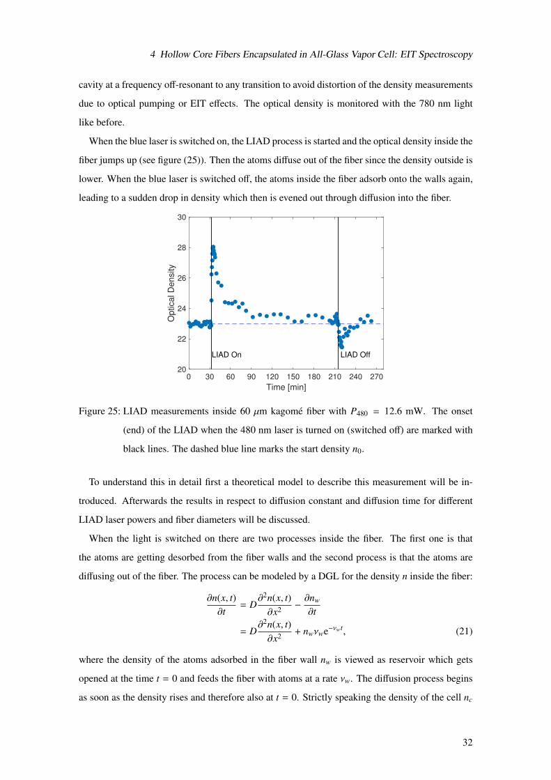
When the blue laser is switched on, the LIAD process is started and the optical density inside the
fiber jumps up (see figure (25)). Then the atoms diffuse out of the fiber since the density outside is
lower. When the blue laser is switched off, the atoms inside the fiber adsorb onto the walls again,
leading to a sudden drop in density which then is evened out through diffusion into the fiber.
0 30 60 90 120 150 180 210 240 270
Time [min]
20
22
24
26
28
30
Optical D
ensity
LIAD On LIAD Off
Figure 25: LIAD measurements inside 60 µm kagome fiber with P480 = 12.6 mW. The onset
(end) of the LIAD when the 480 nm laser is turned on (switched off) are marked with
black lines. The dashed blue line marks the start density n0.
To understand this in detail first a theoretical model to describe this measurement will be in-
troduced. Afterwards the results in respect to diffusion constant and diffusion time for different
LIAD laser powers and fiber diameters will be discussed.
When the light is switched on there are two processes inside the fiber. The first one is that
the atoms are getting desorbed from the fiber walls and the second process is that the atoms are
diffusing out of the fiber. The process can be modeled by a DGL for the density n inside the fiber:
∂n(x, t)∂t
= D∂2n(x, t)∂x2 −
∂nw
∂t
= D∂2n(x, t)∂x2 + nwνwe−νwt, (21)
where the density of the atoms adsorbed in the fiber wall nw is viewed as reservoir which gets
opened at the time t = 0 and feeds the fiber with atoms at a rate νw. The diffusion process begins
as soon as the density rises and therefore also at t = 0. Strictly speaking the density of the cell nc
32
4 Hollow Core Fibers Encapsulated in All-Glass Vapor Cell: EIT Spectroscopy
outside the fiber should rise because of the atoms diffusing outside, but since the volume of the cell
is much larger than the fiber, nc can be approximated to be constant throughout the measurement.
The density n should equilibrate to the same value as before the LIAD. This leads to the boundary
conditions for a fiber of length l of:
n(x, t = 0) = n0 for − l/2 ≤ x ≤ l/2 (22)
n(x = ±l/2, t) = n0. (23)
With this the numerical solution for eq. (21) can be computed. In the case of switching off the
blue light, only the sign in front of the desorption term changes in eq. (21). Now the wall is seen
as a drain and nw is the density of atoms getting absorbed into the fiber wall with the rate νw. Since
the optical density is proportional to the atomic density, this simulation can be transferred directly
to the measurements.
50 100 150
Time [min]
22
23
24
25
26
27
28
29
Optical D
ensity
t85%
= 51.76 min
OD
Theory
(a) P480 = 12.6 mW
50 100 150
Time [min]
22
23
24
25
26
27
28
29
Optical D
ensity
t85%
= 59.23 min
OD
Theory
(b) P480 = 12.6 mW
0 50 100 150 200
Time [min]
22
23
24
25
26
27
28
29
Op
tica
l D
en
sity
t85%
= 49.35 min
OD
Theory
(c) P480 = 6.3 mW
210 220 230 240 250 260
Time [min]
21
21.5
22
22.5
23
23.5
24
24.5
Optical D
ensity
t85%
= 39.90 min
OD
Theory
(d) P480 = 12.6 mW
220 240 260 280 300 320 340
Time [min]
21
21.5
22
22.5
23
23.5
24
24.5
Optical D
ensity
t85%
= 36.69 min
OD
Theory
(e) P480 = 12.6 mW
210 220 230 240 250 260 270
Time [min]
21
21.5
22
22.5
23
23.5
24
24.5
Optical D
ensity
t85%
= 25.86 min
OD
Theory
(f) P480 = 6.3 mW
Figure 26: LIAD measurements in 60 µm kagome fiber for different blue laser powers. The blue
dashed line marks the start density n0 and the end density used for the simulations.
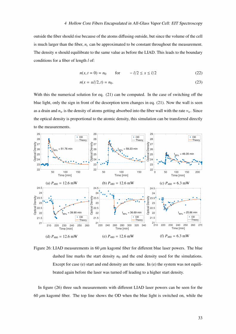
Except for case (e) start and end density are the same. In (e) the system was not equili-
brated again before the laser was turned off leading to a higher start density.
In figure (26) three such measurements with different LIAD laser powers can be seen for the
60 µm kagome fiber. The top line shows the OD when the blue light is switched on, while the
33
4 Hollow Core Fibers Encapsulated in All-Glass Vapor Cell: EIT Spectroscopy
bottom line shows the behavior for the same measurement when the light is switched off again.
Additionally the numerical simulations are shown, whereas D, nw and τw are chosen to fit the
experiment data. In [2] and [3] the “filling time” is defined as the duration until the density inside
the fiber reaches 85% of the surrounding density in equation (14). Following this line of thought
here a time t85% is defined as the time when the difference of n to n0 reaches 1 − 0.85 = 15% of
max(n − n0). These times are also depicted in figure (26).
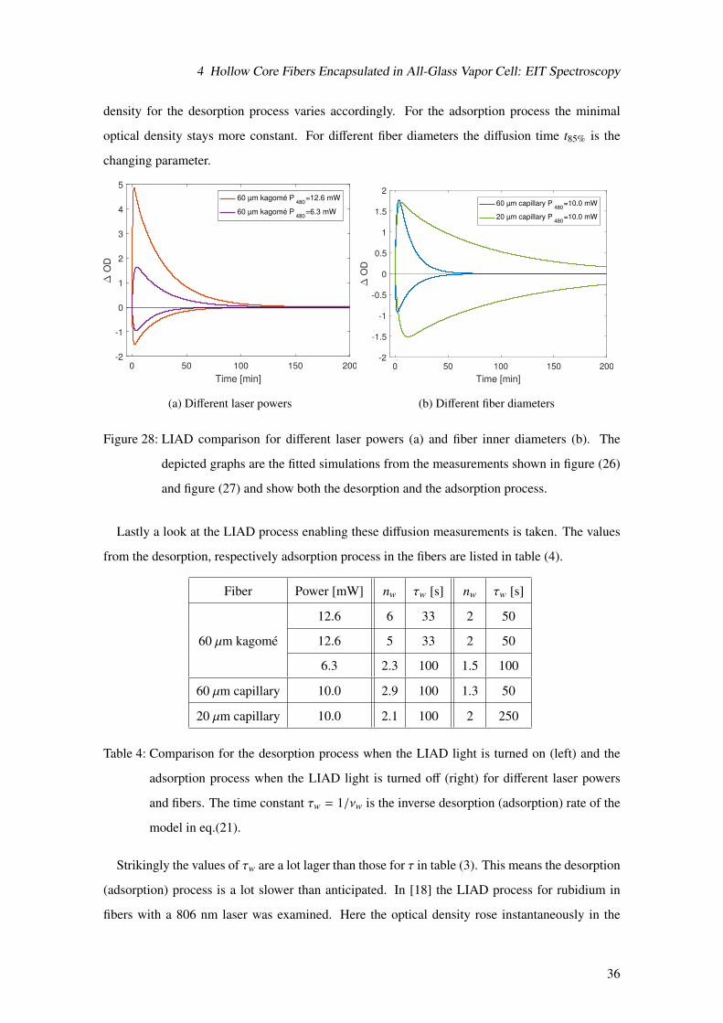
As one can see t85% lies in the range of half an hour to an hour for the 60 µm kagome fiber.
The diffusion process into the fiber surprisingly seems to be faster than out of it. It is however
independent from the LIAD laser power and only nw changes as can be seen in table (4). For half
the laser power the atoms desorbing approximately also halves. The number of atoms absorbing
into the surface when the laser is switched off on the other hand seems to be independent from the
incident laser power. This is plausible since this should only be dependent on the number of atoms
available to adsorb into the fiber wall.
50 100 150
Time [min]
22
23
24
25
26
27
28
29
Optical D
ensity
t85%
= 51.76 min
OD
Theory
(a) 60 µm kagome
0 50 100
Time [min]
10.5
11
11.5
12
12.5
13
13.5
Optical D
ensity
t85%
= 23.91 min
OD
Theory
(b) 60 µm capillary
0 50 100 150
Time [min]
7.5
8
8.5
9
9.5
10
10.5
Optical D
ensity
t85%
= 152.48 min
OD
Theory
(c) 20 µm capillary
210 220 230 240 250 260
Time [min]
21
21.5
22
22.5
23
23.5
24
24.5
Optical D
ensity
t85%
= 39.90 min
OD
Theory
(d) 60 µm kagome
120 140 160 180
Time [min]
9.5
10
10.5
11
11.5
12
Optical D
ensity
t85%
= 24.93 min
OD
Theory
(e) 60 µm capillary
200 250 300 350
Time [min]
6
6.5
7
7.5
8
8.5
9
Optical D
ensity
t85%
= 187.67 minOD
Theory
(f) 20 µm capillary
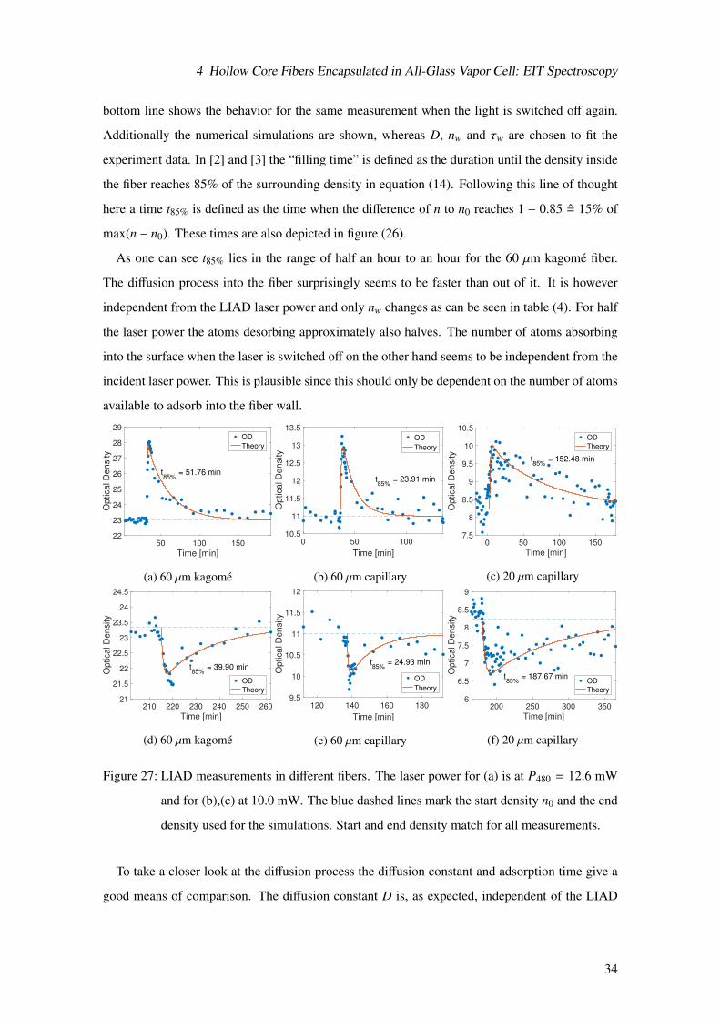
Figure 27: LIAD measurements in different fibers. The laser power for (a) is at P480 = 12.6 mW
and for (b),(c) at 10.0 mW. The blue dashed lines mark the start density n0 and the end
density used for the simulations. Start and end density match for all measurements.
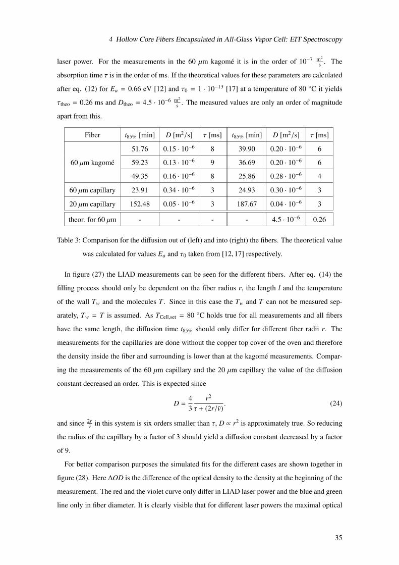
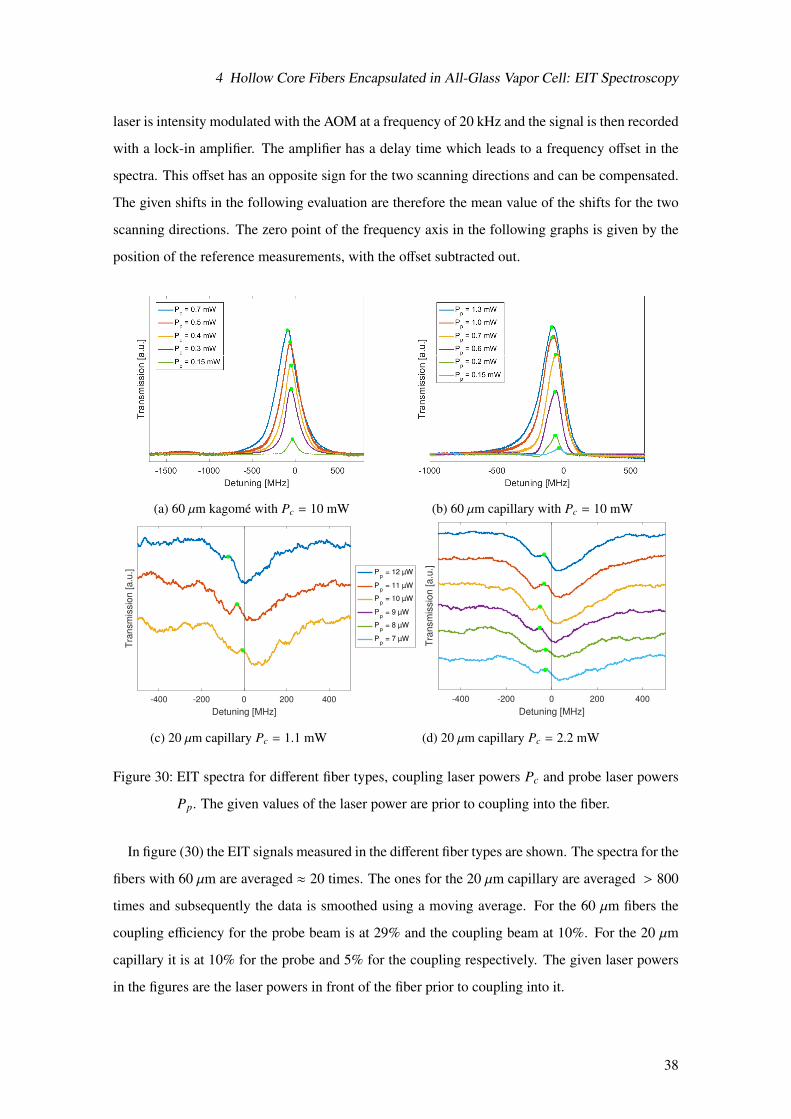
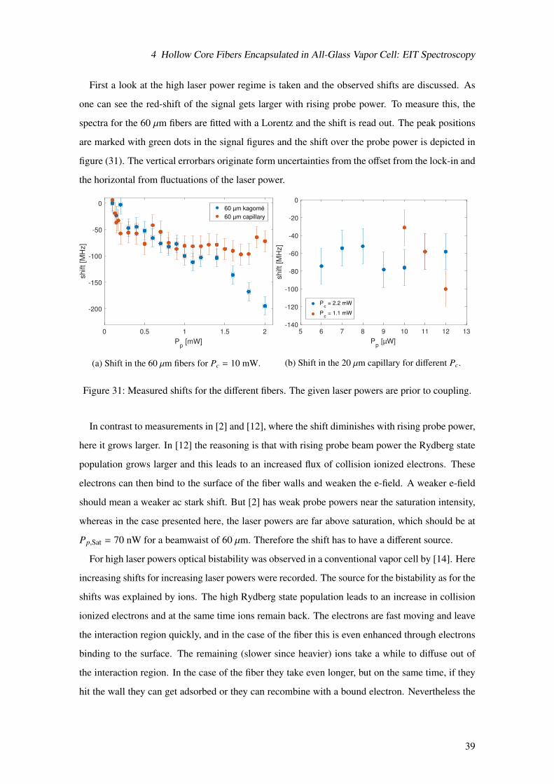
To take a closer look at the diffusion process the diffusion constant and adsorption time give a
good means of comparison. The diffusion constant D is, as expected, independent of the LIAD
34
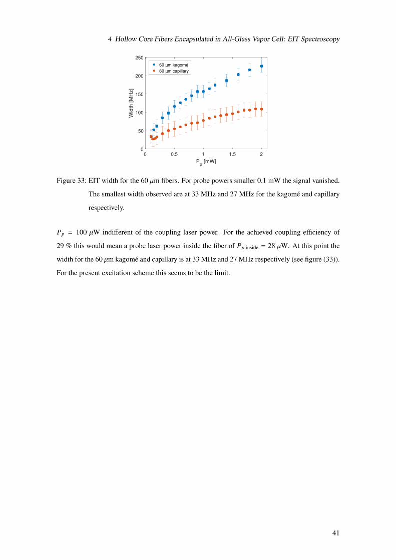
4 Hollow Core Fibers Encapsulated in All-Glass Vapor Cell: EIT Spectroscopy
laser power. For the measurements in the 60 µm kagome it is in the order of 10−7 m2
s . The
absorption time τ is in the order of ms. If the theoretical values for these parameters are calculated
after eq. (12) for Ea = 0.66 eV [12] and τ0 = 1 · 10−13 [17] at a temperature of 80 C it yields
τtheo = 0.26 ms and Dtheo = 4.5 · 10−6 m2
s . The measured values are only an order of magnitude
apart from this.
Fiber t85% [min] D [m2/s] τ [ms] t85% [min] D [m2/s] τ [ms]