Efficient Profiling in the LLVM Compiler Infrastructure DIPLOMARBEIT zur Erlangung des akademischen Grades Diplom-Ingenieur im Rahmen des Studiums Computational Intelligence eingereicht von Andreas Neustifter, BSc Matrikelnummer 0325716 an der Fakultät für Informatik der Technischen Universität Wien Betreuung Betreuer: ao. Univ.-Prof. Dipl.-Ing. Dr. Andreas Krall Wien, April 14, 2010 (Unterschrift Verfasser) (Unterschrift Betreuer) Technische Universität Wien A-1040 Wien Karlsplatz 13 Tel. +43-1-58801-0 www.tuwien.ac.at
Transcript
Efficient Profiling in the LLVMCompiler Infrastructure
DIPLOMARBEIT
zur Erlangung des akademischen Grades
Diplom-Ingenieur
im Rahmen des Studiums
Computational Intelligence
eingereicht von
Andreas Neustifter, BScMatrikelnummer 0325716
an derFakultät für Informatik der Technischen Universität Wien
BetreuungBetreuer: ao. Univ.-Prof. Dipl.-Ing. Dr. Andreas Krall
Wien, April 14, 2010(Unterschrift Verfasser) (Unterschrift Betreuer)
Technische Universität WienA-1040 Wien � Karlsplatz 13 � Tel. +43-1-58801-0 � www.tuwien.ac.at
Andreas Neustifter, BScUnterer Mühlweg 1/6, 2100 Korneuburg
Hiermit erkläre ich, dass ich diese Arbeit selbständig verfasst habe, dass ich die verwendetenQuellen und Hilfsmittel vollständig angegeben habe und dass ich die Stellen derArbeit—einschließlich Tabellen, Karten und Abbildungen— die anderen Werken oder dem Internetim Wortlaut oder dem Sinn nach entnommen sind, auf jeden Fall unter Angabe der Quelle alsEntlehnung kenntlich gemacht habe.
In computer science profiling is the process of determining the execution fre-quencies of parts of a program. This can be done by instrumenting the programcode with counters that are incremented when a part of the program is exe-cuted or by sampling the program counter at certain time intervals. From thisdata it is possible to calculate exact (in the case of counters) or relative (inthe case of sampling) execution frequencies of all parts of the program.
Currently the LLVM Compiler Infrastructure supports the profiling of pro-grams by placing counters in the code and reading the resulting profiling dataduring consecutive compilations. But these counters are placed with a naıveand inefficient algorithm that uses more counters than necessary. Also therecorded profiling information is not used in the compiler during optimisationor in the code generating backend when recompiling the program.
This work tries to improve the existing profiling support in LLVM in severalways. First, the number of counters placed in the code is decreased as presentedby Ball and Larus [19]. Counters are placed only at the leaves of each functionscontrol flow graph (CFG), which gives an incomplete profile after the programexecution. This incomplete profile can be completed by propagating the valuesof the leaves back into the tree.
Secondly, the profiling information is made available to the code generatingbackend. The CFG modifications and instruction selection passes are modifiedwhere necessary to preserve the profiling information so that backend passesand code generation can benefit from it. For example the register allocator isone such backend pass that could benefit since the spilling decisions are basedon the execution frequency information.
Thirdly, a compile time estimator to predict execution frequencies when noprofiling information is available is implemented and evaluated as proposed byWu et.al. in [71]. This estimator is based on statistical data which is combinedin order to give more accurate branch predictions as compared to methodswhere only a single heuristic is used for prediction.
The efficiency of the implemented counter placing algorithm is evaluated bymeasuring profiling overhead for the naıve and for the improved counter place-ment. The improvements from having the profiling information in the codegenerating backend is measured by the program performance for code whichwas compiled without and with profiling information as well as for code thatwas compiled using the compile time estimator.
2
Kurzbeschreibung
Unter Profilen versteht man in der Informatik die Analyse desLaufzeitverhaltens von Software, meist enthalten diese AnalysedatenAusfuhrungshaufigkeiten von Teilen eines Programms. Diese Haufigkeitenkonnen entweder durch das Einfugen von Zahlern im Programm bestimmtwerden oder dadurch, dass der Programmzahler periodisch aufgezeichnetwird. Uber diese gemessenen Haufigkeiten fur einige Programmteile kann dieAusfuhrungshaufigkeit aller Programmteile berechnet werden.
Derzeit unterstutzt die LLVM Compiler Infrastruktur die Analyse von Pro-grammen, indem Zahler in den Programmcode eingefugt werden, die Ergeb-nisse der Zahler konnen dann bei spateren Ubersetzungen verwendet werden.Diese Zahler werden aber ineffizient und naıv eingefugt, dadurch werden mehrZahler verwendet als notwendig sind. Außerdem wird zur Verfugung stehendeProfilinformation wahrend der erneuten Ubersetzung des Programms nichtverwendet.
In dieser Arbeit wird die bestehende LLVM Profiling Unterstutzung folgen-derweise verbessert: Erstens wird die Anzahl der Zahler, die in dem Pro-grammcode eingefugt werden, auf das Mindestmaß reduziert (Ball und Larus[19]). Dies wird dadurch erzielt, dass, ausgehend von den wenigen eingefugtenZahlern, die Ausfuhrungshaufigkeiten von allen Programmteilen bestimmt wer-den.
Zweitens wird die Analyseinformation so aufbereitet dass der Compiler beieiner Neuubersetzung des Programms diese Informationen verwenden kann.Alle CFG-modifizierenden Teile des Compilers und der Codegenerierungsteilwerden angepasst um diese Informationen zu erhalten und zu verwenden. ZumBeispiel kann der Registerallokator die Profilinformation verwenden um dieEntscheidung, welche Register in den Speicher ausgelagert werden sollen, zuunterstutzen.
Drittens soll ein Schatzalgorithmus implementiert und getestet werden, derwahrend der Ubersetzung eines Programms Ausfuhrungshaufigkeiten ab-schatzt, falls keine Profilinformation zur Verfugung steht (Wu et.al. [71]).Dieser Schatzalgorithmus basiert auf den Laufzeitdaten mehrere Programme,wobei diese Daten mit statistischen Methoden kombiniert werden. Es solluberpruft werden, ob diese Kombination im Vergleich zu der Verwendungeinzelner Datenpunkte sinnvoll ist, und ob sie das tatsachliche Laufzeitver-halten des Programms besser abbildet.
Die Effizienz des implementierten Algorithmus zum Einfugen von der Min-destanzahl an Zahlern wird evaluiert, indem der Overhead der naıven Im-plementierung mit dem der Neuimplementierung verglichen wird. DieVerbesserung der Codegenerierung durch Einbeziehung der Profilinformation
wird durch Performancevergleiche zwischen Code, der ohne und mit Profilin-formation ubersetzt wird, getestet.
4
For the fashion of Minas Tirith was suchthat it was built on seven levels,each delved into a hill,and about each was set a wall,and in each wallwas a gate.
J.R.R. Tolkien, ”The Return of theKing”
(In [51] when referring to systemoverview.)
Chapter 1
Overview
This chapter gives an overview on this thesis and on the topics covered. Asurvey of the available literature and the known algorithms is done and thegoals of this work are established.
Chapter 2 provides a detailed look on profiling and on some of the algorithmsused later on, it also establishes some nomenclature. Chapter 3 introduces theLow Level Virtual Machine (LLVM) in more detail, the LLVM is a compilerinfrastructure that was used to implement several of the profiling algorithms.Chapter 4 covers the implementation of the profiling algorithm in LLVM anddiscusses some of the more challenging problems and their solutions. Chapter5 finally presents the results of this thesis: analysis on the algorithms efficiencyand measurements on the SPEC2000 Benchmark.
1.1 What is profiling?
Profiling is the act of generating a profile for a piece of software, the termprofile describes some sort of characteristic information. As an example theoverall execution time for each function in a program (for one execution ofthe program) is such a characteristic information. As early as 1965 there wereattempts to generate runtime profiles for programs, at this time the behaviourof a CPU was recorded by another CPU and written to tape [12].
Donald Knuth first used the term profile when he analysed how often cer-tain FORTRAN statements where executed during the run of the program[52]. In Knuth’s case the profile described execution counts per statement.Knuth already anticipated that this kind of information is extremely valuableto programmers, since they can easily pin-point performance bottlenecks. Forexample the “execution counts per statement”-profile can help the program-mer to find the statements that are executed most frequently, usually thisstatements offer the most potential for runtime optimisations.
5
Today the term profile is more widely used to describe a certain characteristicthat is attached to some part of a program. This could be for example “ex-ecution counts per statement”, “cache misses per function”, “execution timeper statement” or some other type of information.
1.2 Profiling in the Literature
The first attempts to collect information on the runtime characteristics ofprograms were made in the late 1960’s by C.T.Apple at IBM with the ambitiousgoal to record the instruction trace of an IBM 7090 [12]. Although it was notpossible to record all instructions they managed to sample enough data to gainan overview on the runtime characteristics of the programs in question. Thenthe parts of the program where it spent most of its runtime were optimised,this improved the programs runtime significantly with minimal effort from theprogrammer.
With the advent of compiler optimisations [5, 33, 59] the need to do automatedanalysis of the programs to assist the optimiser [7, 34] became more apparent.But it was also important to determine areas in which the compiler producedsuboptimal code so that new and better optimisations could be found.
This prompted Knuth in 1970 [52] to do a big analysis of FORTRAN codeto determine which statements and constructs where used most frequently by(FORTRAN-)Programmers at that time. He developed a program called FOR-DAP that instrumented a FORTRAN program to record execution counts.When he then optimised the code at the found hot-spots in the program (state-ments that where executed very often) the execution time of the program wascut down to a fourth of the runtime of the original program.
FORDAP instrumented the whole code, each basic block had a counter at-tached, this added some redundant counters which resulted in an unnecessaryhigh profiling overhead. This problem was tackled and solved also by Knuthtwo years later in his seminal paper ”Optimal measurement points for programfrequency counts” [53] in which he proved how a minimal number of counterscan be placed which still provide execution counts for all parts of the program.
Up to this time every part of a program was instrumented, but Knuth instru-mented only parts of the code, the profiling information for the other partswas calculated off-line after the program had been run and the profiling infor-mation was recorded. Since fewer counters were placed in the program, thisalso reduced the profiling overhead. In 1981 Forman [42] reduced the overheadeven more by placing this counters in parts of the program that were less likelyto be executed by describing one of the first static profile estimators.
Also at that time Graham [44] introduced gprof, a successor to the widelyused Unix tool prof (that provided sample based execution time profiling).
6
The novelty of gprof was that it provided not only the raw times which wherespent in a method, but it took into consideration the call graph and attributedthe time of called methods to the callee. This gave timing profiles a newpurpose since it was not only possible to see where the most time was spentbut also why this happened, e.g. which callers were using the callee most ofthe time.
In 1988 Aral and Gertner [13] introduced Parasight which used parallel proces-sors by offloading the profiling process to a separate processor thus adding thepossibility to profile parallel applications and reducing the profiling overheadwhile profiling several other processors. They further reduced the overhead byonly selectively profiling parts of the program, using an interactive process to“zoom in” on the areas of interest.
In 1990 Larus [55] tackled the problem of tracing programs where the goal isnot only to know how often a statement was executed but also what the previ-ous execution history was at that time. So for each execution of a program thesuccession of executed basic blocks is recorded, providing hot path informationfor the functions of the program. Larus did this efficiently by analysing theC-code and placing probes only where the code was non deterministic. Thisresulted in incomplete traces that were completed by executing the determin-istic parts of the program again to provide the full trace, this technique wascalled abstract execution.
In 1992 Fisher and Freudenberger [41] profiled several big projects and showedthat for a given branch the branching probabilities where almost the same fora wide range of input data, suggesting that a well sampled set of input datacan be used as branch predictors.
Ball and Larus [18] compared several static branch prediction heuristics in1993 and used an ordering of these heuristics to improve the overall accuracy,but only Wu and Larus [71] in 1994 managed to combine these heuristics withstatistical methods to do accurate static branch prediction.
In 1994 Ball and Larus [19] first implemented Knuth’s “minimal number ofcounters”-algorithm and provided an off-line tool that completed the recordedbasic block or CFG edge profiling information. They presented a simple profileestimator that aimed at reducing the runtime overhead of the profiling codeby placing the counters in less likely executed regions of the program. Theyalso showed the complexity relations between basic block and edge profilingand that edge profiling is as efficient as block profiling while providing moregranular data.
Ball and Larus then also tackled the tracing (path profiling) problem andshowed in 1996 [20] how to place trace probes into the program while minimis-ing the overhead. They achieved this by enumerating all unique paths from thefunctions entry block to its exit and placing code along the paths that addedup a number. The resulting number at the end of the function was equal to
7
the unique number of the taken path, these numbers where stored and couldlater be used to analyse which paths were taken during the execution.
Anderson [10] showed in 1997 how to profile a whole system by adding sam-pling code to the kernel and an user mode daemon that processed the kernel-generated data. With this system it was possible to profile all running pro-grams in a running system and to determine which programs and libraries usedthe most system resources.
Also in 1997 a completely different approach to profiling was chosen byCalder et. al. [27]. They profiled the values of variables trying to determinepossible optimisations based on this value information.
1.3 Goals
The goals for this thesis were threefold:
• Implement the optimal instrumentation algorithm for measuring execu-tion counts in LLVM. This includes writing a crude flow-based staticestimator that guides the counter positioning, as well as the instrumen-tation itself and a small helper program to display the annotated code.
• Provide the profile information to the code generating backend, so thate.g. the register allocator can use this information.
• Implement an estimator that combines several heuristics to calculate astatic profile that can be used as guidance for the backend in case nodynamic (runtime) profile is available.
Although LLVM already had a small instrumentation framework implementedthat provided the base for the new implementation, the old framework wasquite buggy and unmaintained, so essentially the whole framework was rewrit-ten from scratch.
Providing the profile information for the backend poses some great difficul-ties since the control flow graph is modified heavily during optimisation andcode generation so maintaining consistent profiling information was and is achallenge.
During the work on the first two points the heuristics based estimator wasalready implemented by Andrei Alvares [8], so this thesis only contains a dis-cussion of the algorithm.
8
Therefore whosoever heareth thesesayings of mine, and doeth them, I willliken him unto a wise man, which builthis house upon a rock.
Matthew 7,24(From the King James Version of the
Bible.)
Chapter 2
Profiling
This chapter establishes the basics of profiling and introduces some importantalgorithms. In Section 2.1 the basics of profiling are discussed, Section 2.2presents the methods for recording profiles during the runtime of a program.Section 2.3 covers some of the static profiling algorithms and finally Section2.4 presents the algorithms used for dynamic profiling.
2.1 Basics
Profiling describes acquiring certain information from a program, this infor-mation is called a profile. Depending on the type of profile this informationcan, for example, be used to
• improve the program specifically in the areas shown to be problematicby the profiling information,
• determine the test coverage of the input data and/or
• provide different input to the program so that different paths in thecontrol flow graph are executed and tested.
The profile information can be associated with certain parts of a program, withfunctions, call graph edges, basic blocks or control flow graph edges.
The following sections describe certain aspects of profiles, Section 2.1.1 explainsthe difference between dynamic and static profiles. Section 2.1.2 takes a look atdifferent types of profiling information and Section 2.1.3 covers the granularityof profiles.
9
2.1.1 Dynamic versus Static Profiles
With dynamic profiling the information is recorded during the runtime of theprogram. A profile can contain information from several different executionsof a program. With static profiling the information is obtained purely byanalysing the program, (e.g. during compile time).
Dynamic Profiling
Dynamic profiling is more accurate than static profiling, since it does not relyon estimates but accurately captures the information when the program isexecuted. On the down side this approach imposes a runtime overhead, theprogram runs at lower than usual speed because capturing the profile alsoneeds some of the runtime resources. This can be especially problematic forreal-time applications.
Another disadvantage is that the recorded profile is dependant on the inputused to run the program. When the used input is not a representative sampleof the possible real-world inputs it is likely that the profile does not accuratelycapture the average runtime behaviour of the program. This can be partlyovercome by combining the profiles of several executions with different inputdata into a single profile.
Static Profiling
In contrast to dynamic profiles, which are obtained by running the programand measuring certain characteristics, static profiles are determined by algo-rithmically analysing the program (without executing it). For some types ofprofiling information (e.g. cache misses) this is hard or impossible to do.
Since those static profiles usually are only estimates, they have different prop-erties than dynamic profiles:
• Most interesting programs show a non-deterministic behaviour, that istheir execution depends on some external factors like input or time. Fornon-deterministic programs a static profiling algorithm can only providerelative values (for a discussion of relative and absolute profiles see Sec-tion 2.2.2). Although it is theoretically possible to calculate absoluteprofiles for deterministic programs, the required data flow analysis issometimes hard to do, thus making absolute static profiles impractical.
• Static profiles are not dependant on input, if the profiling algorithm isdeterministic, then the static profiling information is deterministic too.
Often static profiles are used during the compilation of programs to help thecompiler with certain decisions. E.g. the complier can use an execution count
10
estimate to help the register allocator make its spilling decisions.
For each algorithm a measure of efficiency and correctness can be established.This measures can then be used to compare algorithms and may help choosingthe right algorithm for a given task. This also holds true for static profilingalgorithms (often called estimators in the remainder of this work). For esti-mators the most important measure is, how well the produced estimates are.This can be determined by generating a dynamic profile with the same charac-teristics as the static one (relative/absolute, type, granularity) and comparingthose two profiles.
2.1.2 Types of Profiling Information
There are many types of profiling information that can be derived from aprogram. Some of the common profiling types (amongst others) are:
Execution Counts For a given part of the program it is recorded how oftenthis part was executed. This is one of the easiest profiles to obtain, al-though when done inefficiently it poses a considerable runtime overhead.
Execution Times This records how long the CPU spent executing a givenprogram part. It is difficult to capture this information accurately sincethe measurement itself needs some of the CPU time and thus influencesthe measurement.
Cache Misses, Number of Branch Mispredictions,
Pipeline Stalls This records how often, in a given part of the program, acache miss/branch misprediction/pipeline stall occurred, this is usuallymeasured with the help of hardware counters.
2.1.3 Granularity of Profiling Information
Profile information associates a certain piece of information (usually a number)with a certain part of the program. Usually those parts of a program are (inorder of increasing granularity):
Functions For each function one counter/timer is stored.
Call Graph Edges When a function calls another function an edge in thecall graph is added to represent this and profiling information is attachedto this edges. So for example not only the number of invocations of afunction is recorded but how often each callee invoked the function.
Basic Blocks A basic block is a sequence of instructions without branches.So, given the first instruction is executed all other instructions in theblock are also executed.
11
Control Flow Graph Edges When a basic block ends it either returns thefunction or branches to one or more basic blocks, those branches are theedges of the control flow graph.
Statement Each statement has profiling information attached to it.
Instruction Usually each statement consists of several instructions. It ispossible to measure some types of profiling information on the instructionlevel.
Depending on the type of profiling information, it may be possible to inferinformation for a lower granularity item by looking at information of highergranularity. For example the execution count of a function can be derived fromthe execution count of the first basic block (the entry block) of this function.The execution count of the entry block in turn can be determined by the sumof all CFG edge counts that leave the entry block.
2.2 Methods for Dynamic Profiling
Static profiling is done without running the program, so it does not matter (aslong as the profiler terminates) how long this process takes. Dynamic profilingon the other hand is done during the runtime of the program so it is desirablefor the overhead this profiling imposes to be as low as possible. (Since usuallyit is necessary that the software runs at a certain minimum speed the overheadmust not exceed a certain level).
The problem of keeping the overhead low while still acquiring accurate profilinginformation was tackled with different means. When instrumenting the codewith counters (sometimes called probes) the number and placement of thosecounters was optimised. Also the profiling accuracy was traded against lowerruntime overhead by using sampling instead of instrumenting the source code.
2.2.1 Instrumentation
Instrumentation describes the process of adding code, that performs the record-ing and storing of profiling information, to a program.
A Small Example
When the execution frequencies of each CFG edge have to be measured, theprogram is modified so that upon traversal of such an edge at runtime a counteris incremented. Additionally, at the start of the program, an auxiliary functionis called that initializes all the counters. At the end of the program the countersare written to a file, if the file exists already it is common practice to either
12
add the new values to the already stored ones or to append the new counts,this automatically aggregates counts from several executions of the programinto a single profile information file.
Instrumentation in General
The instrumentation itself can be done at several stages during the programlifetime:
Source Code To instrument the source code, all the code has to be parsedand instrumentation code has to be placed at the necessary points.
Compile Time During compile time, before invoking the code generatingbackend the intermediate representation is instrumented.
Binary Modification The executable binary is directly modified to add thenecessary instrumentation code.
Run Time Some frameworks allow the dynamic addition of profiling codeduring the runtime of a program.
Source code and compile time instrumentation both have the advantage ofbeing machine independent, but this also means that it is harder for them touse processor specific hardware counters. Binary modification on the otherhand is inherently machine dependent so it has the advantage of being ableto use hardware counters much easier, but porting it to different hardware ismuch harder.
Also, for source code and compile time instrumentation the source code has tobe available to be able to instrument programs. This can be a problem whenclosed source binary programs have to be analysed, binary modifications donot have these limitations.
Compile time instrumentation has the advantage that all the information nec-essary to instrument the code is readily available and only a small amount ofadditional information has to be gathered before the instrumentation. Sourcecode and binary instrumentation on the other hand usually have to analyse theprogram from scratch to find out where to place instrumentation code beforedoing the actual instrumentation.
Advantages of Instrumentation
Instrumenting a program and executing the resulting binary gives exact profilesthat are reproducible with each renewed execution of the program (providedthe input is the same and the program otherwise has deterministic behaviour).
13
Since the profiling information is exact, it can be also used for test coverage orcontrol flow analysis, since it is possible to tell whether or not a certain CFGpath was executed.
Disadvantages of Instrumentation
Instrumentation usually has a larger runtime overhead than sampling (seeSection 2.2.2).
2.2.2 Sampling
With sampling the executable binary is not modified to gather profiling in-formation, instead the program is halted and resumed during its execution(usually via timed interrupts) to record various properties of the current state.This halting/recording/resuming has to be done with a precise periodicityotherwise the measured values could be biased towards certain parts of theprogram.
Sampling is usually done with a profiling program that executes and halts theprofiled program as needed and records the measured results but it is alsopossible to modify the program to directly contain this profiling code. Witha multi-core system it is also possible to monitor the program on-the-fly via amonitoring routine that runs on a separate core.
Since the profiling information is only sampled at certain points in time, theprofiling information is not composed of absolute numbers but contains relativevalues instead. E.g. if the real execution count for Function 1 is 10 and forFunction 2 it is 120 then maybe the measured counts are 3 and 40. It is notpossible to say how often Function 1 or Function 2 have been executed, but itis possible to say that Function 2 was executed approx. 12 times as often asFunction 1.
Advantages of Sampling
Sampling does not require the program to be changed, but for interpretingthe measurements it is useful to have debugging information available for thebinary, or to be able to translate the program with debugging information en-abled. Also, with a sensible profiling frequency or when using a second core orprocessor, the runtime overhead is lower than the overhead of instrumentation(see Section 2.2.1).
14
Disadvantages of Sampling
Sampling only provides relative information, it is not possible to tell how oftena certain event occurred exactly. Depending on the task at hand this may ormay not be sufficient: e.g. when it is necessary to find out where a programspends most of its time the relative execution frequencies are suitable. But fordetermining the test coverage of a function relative counts are not enough toensure that every edge in the CFG was executed at least once.
Since sampling can miss certain events it is not possible to say that e.g. abasic block was never traversed during the execution of a program. It is justas well possible that the sampling never occurred at the time the block wasexecuted.
2.2.3 Hardware Counters
Hardware counters where first introduced in the early 1990’s and by the mid1990’s all major CPU manufacturers (most notably Cray but also SiliconGraphics, Intel, IBM, DEC, SUN and HP [74]) implemented hardware perfor-mance counters in their microprocessors. This wide availability of performancecounters triggered a wide variety of new dynamic profiling implementationsthat did not rely on instrumentation but instead used these new hardwarecounters to measure the performance of programs.
Usually these processors had support for certain types of events such as “cycleexecuted“, ”instruction issued“, ”store issued“, ”branch mispredicted”, “cachemiss”,. . .
In most implementations not all of these events could be counted at once due tohardware restrictions. There where one or two (seldom more) counter registersthat could be configured to count only one of those events. For example theSGI MIPS R10000 had two counters that could be configured to capture twoout of 16 event types [74].
Since most programs run on several different hardware platforms it was hard forapplication- and tool-developers to use this performance counters in a hardwareindependent way. Several projects aimed on unifying this hardware interfacesinto a common API:
Performance Counter Library (1998-2003) The PCL was the first at-tempt to create an unified API for accessing the hardware performancecounters on several different hardware platforms.
perfctr (2002-current) Linux kernel drivers that present a large number ofdifferent hardware counters from different platforms as common inter-face.
15
perfmon (2002-current) Initially developed by HP perfmon is a kernelmodule for Itanium, x86 64 and ppc64 architectures that exposes a com-mon API for those hardware counters.
PAPI (1999-current) The Performance API further virtualises the hard-ware performance counters by providing a completely system indepen-dent API while relying on e.g. perfctr and perfmon to actually accessthe hardware counters. It not only spans a multitude of processors butalso supports a large number of operating systems such as Linux, AIX,Unicos and Solaris.
PerfSuite (2003-current) A project that focuses on making hardware pro-filing not only work but also easy and reliable to use, it relies on PAPI,perfmon and perfctr for data acquisition and Graphviz for data repre-sentation.
2.3 Static Profiling Algorithms
This section covers the algorithms for creating static profile estimations, Sec-tion 2.3 covers a simple estimator and Section 2.3.2 a more sophisticated one.Finally Section 2.3.3 discusses intra-procedural profile estimation.
2.3.1 A Naıve Execution Count Estimator
This heuristic was introduced by Ball and Larus in 1994 [19] and is still widelyused in compilers today. It estimates edge execution frequencies for a singlefunction, but the results can also be used to perform program wide estimateswhen the results are propagated along the call graph as described in Section2.3.3.
The basic principle is this: the deeper an edge is nested in conditional branches,the less likely this edge is executed. Also, an edge that is inside a loop is likelyto be executed more often, Algorithm 1 gives a short overview.
The algorithm starts by determining the back edges and loop headers of afunction by performing a loop detection algorithm that generates informationon the natural loops in a function.
The natural loop (as defined by Aho [2]) of a back edge (v2, v1) is defined as
nat loop((v2, v1)) = {v1} ∪ {v|there is a directed path from v to v2
that does not include v1} (2.1)
The natural loop of a loop head nat loop(v) is the union of all natural loops ofback edges ending in v. The definition of natural loops leads to the property
16
that, if va and vb are loop heads, then the natural loops of va and vb are eitherdisjoint or one is completely contained in the other. This also makes it possibleto define loop exits of a loop header:
In a second traversal of the control flow graph the edge and block weights arecalculated with the following rules, assuming that loops are executed loop multtimes:
1. The incoming weight wi of a basic block is the sum of the weight ofall incoming edges that are not back edges. For the entry block of thefunction (which has no incoming edges) the weight is assumed to be 1.
2. If the basic block v is a loop head with incoming weight wi and the num-ber of loop exit edges n = |loop exits(v)| then each edge in loop exits(v)gets weight wi/n.
3. If the basic block v is a loop head then the weight of the block is wv =wi∗ loop mult, otherwise it is wv = wi. If wl is the weight of the loop exitedges directly leaving the block and n is the number of other edges leavingthe block, then the weight for each of this other edges is (wv − wl/n).
So the algorithm assumes that, if the control flow graph splits up into n pathsin a non-loop-header block, each outgoing edge is 1/n as likely to be executed asthe basic block itself. Additionally the algorithm assumes an average numberof loop executions and multiplies the likelihood of the loop header and itsoutgoing edges by a factor loop mult.
2.3.2 A Sophisticated Execution Count Estimator
In 1994 Wu and Larus [71] presented an estimator that combines several pre-dictions regarding the outcome of a branch to make more accurate estimations.The algorithm relies on real world programs that are profiled first, this pro-grams and their profiling data is then analysed and the collected results areused during the estimation of arbitrary programs.
For the analysis several categories were established and the branches in theanalysed programs then would fall into one or more of these categories:
• Branches that either take a back edge to the loop head or to a blockoutside the loop.
• Branches based on comparisons (e.g. between pointers, on pointer isnull,. . . )
• Branches based on the contents of the next basic block (e.g. is onebranch target a loop header, does one branch target contain a call, doesthe branch target return,. . . )
17
Algorithm 1 NaiveEstimator(P )→ W
for all functions f in program P dofor all blocks b in function f do
determine back edges(b) and is loop head(b)determine nat loop(b)determine loop exits(b) edges
end forfor all blocks b in function f do
if b is the function entry block thenwi := 1
elseei := {(a, b)|(a, b) /∈ back edges(b)} // incoming edgeswi :=
∑e∈ei we
end ifif is loop head(b) then
for all e ∈ loop exits(b) dowe := wi
|loop exits(b)|end forwb := wi ∗ loop mult
elsewb := wi
end ifel := {(b, c)|(b, c) ∈ loop exits(b)}wl :=
∑e∈el we // exit edges already have weight
eo := {(b, c)|(b, c) /∈ loop exits(b)} // outgoing edgesfor all e ∈ eo do
we := (wb−wl)|eo|
end forend for
end for
18
Additionally dynamic profiles of the real world programs were measured. Thismeasured values were used to determine the probability that, given a branchfalls into one of the categories, the branch is actually taken. This results inseveral heuristics, for example if a branch is based on a comparison of a pointerto null, the probability that the branch is taken is 60%. Or if the block thatis branched to returns the function the probability for it to be taken is 72%.
When analysing a program the algorithm determines for each branch intowhich of the categories it falls. When the branch falls into more than onecategory, the possibilities of the heuristics for this category are combined withstatistical methods to estimate the overall probability that this branch is taken.
When using those estimated branch probabilities to estimate execution fre-quencies for all of the control flow edges and basic blocks care has to be takenwhen the function contains loops. Wu and Larus thus also presented a methodto calculate this execution frequencies from local branch probabilities whichworks for reducible control flow graphs. (Reducible CFGs are graphs wherethe loop head dominates all blocks in the loop see [71] for details.)
2.3.3 Estimators for Call Graphs
The previous two estimators (Sections 2.3.1 and 2.3.2) are concerned withthe estimation of (relative) execution counts inside one function. Having thatinformation it is also possible to estimate the execution counts for functionsand for the edges in the call graph of a program, this method is also presentedin [71].
When a function f calls a function g multiple times, then the local call fre-quency lfreq(f, g) is the sum of the execution frequencies of each block b thatcalls g. The global call frequency (for f calling g) is the local call frequencytimes the number of invocations of f .
Assuming that cfreq(f) is the number of invocations of f and gfreq(f, g) isthe global call frequency of f calling g then:
• if f is the main function: cfreq(f) = 1
• if f is not the main function:
cfreq(f) =∑
p∈pred(f)
lfreq(p, f)
•
lfreq(f, g) =∑
{b∈f |b calls g}
freq(b)
• gfreq(f, g) = lfreq(f, g)cfreq(f)
19
2.4 Dynamic Profiling: Optimal Counter
Placement
In this section an algorithm is presented that instruments a program with theminimal possible amount of edge counters.
2.4.1 Overview
When instrumenting a program to measure execution counts, it is possible tosimply attach a counter to every edge in the program. Unfortunately this isinefficient and imposes an unnecessary high runtime overhead onto the pro-gram.
To get rid of the redundant counters Knuth in 1973 [53] devised a method foronly placing counters on certain edges in the CFG. The generated dynamicprofile was incomplete (only for edges with an attached counter the executioncounts were known) but an off-line algorithm which was running later on wasused to calculate the execution counts for the edges which had no counterattached. Knuth was also able to show that his method only inserted theminimal necessary amount of counters. Starting on page 25 the proofs aregiven that Knuth’s method is indeed optimal by showing that the number ofinserted edges is sufficient and necessary. Sufficient means that really onlythose edges are needed to profile the function and necessary means that all ofthese counters are necessary, when removing one the profiling is not completeany more.
The algorithm (see Algorithm 2) operates on each function by first calculatinga spanning tree of the control flow graph. All edges that are not in the spanningtree (edges attached to a leaf node) get a counter attached. After the programhas been executed the profile is completed by calculating the execution countsfor the edges of the spanning tree itself (Algorithm 3). Since each leaf node hasedges attached to it that are associated with a counter and thus have profilingvalues, the execution count for the leaf node itself and the edge connecting itto the tree can be determined.
The runtime behaviour for the instrumented program can be further improvedby placing the counters on edges that are less likely to be executed. Thiscan be done by estimating a profile in some way (see Section 2.3) and thencreating a maximum spanning tree using the estimated edge weights insteadof an arbitrary spanning tree.
20
Algorithm 2 InsertOptimalEdgeProfiling(P )→ Pi
create array C in Pindex := 0for all functions f in program P do
// calculate the spanning tree for fST := ∅for all edges e in function f do
if adding e to ST does not create a cycle in ST thenST := {e} ∪ ST
end ifend for// add counters to Pfor all edges e in function f do
if e /∈ ST thenadd code to P such that {C[index] + +} is executed when e is traversedadd code to P that initialises C[index] with 0
elseadd code to P that initialises C[index] with −1
end ifindex + +
end foradd code to P that writes counter array to file at end of execution of P
end for
Algorithm 3 ReadOptimalEdgeProfile(P, Profile)→ W
read array C from Profileindex := 0for all functions f in module P do
// read profiling informationfor all edges e in function f do
we = C[index]index + +// when the edge had no counter attached, add it to open setif we == −1 then
O = {e} ∪Owe = −1
end ifend for// recalculate counter for edges in open setwhile |O| > 0 do
for all e ∈ O doif either end of e has no adjacent edges in O then
calculate we from weights of adjacent edgesend if
end forend while
end for
21
2.4.2 Example
In Figure 2.1 a CFG with an optimal edge profiling instrumentation is shown.First Algorithm 1 determines the given estimation of the edge weights thenthe maximum spanning tree is calculated resulting in the tree with the dashededges. (The edge (0, entry) and (return, 0) are virtual edges that are requiredby the algorithm to optimally instrument the CFG (for details on these edgessee Section 2.4.3)). The solid edges, the ones that are not in the MST, arefitted with counters.
In Figure 2.2 a measured profile of the program is given. Of course only thesolid edges had counters attached, so only these edges are really measured.The other edges are calculated according to Algorithm 3:
• Edge (bb3, bb5) has weight 75, edge (bb4, bb5) has weight 6, so edge(bb5, bb6) has necessarily weight 81. From these two edges also the edges(bb2, bb3) (weight 75) and (bb2, bb4) (weight 6) can be calculated.
• Edge (bb6, bb2) can be calculated from (bb2, bb3) and (bb2, bb4).
• Edge (bb7, bb9) gives the flow for (bb6, bb7), this edge, together with(bb6, bb2) and (bb5, bb6) can be used to calculate (bb1, bb6).
• . . .
2.4.3 Virtual Edges
The algorithm assumes that a function has a single entry and exit point, thosetwo points are conceptually connected via a virtual edge. This edge creates acycle that is also broken by the algorithm (see Section 2.4.5) so either the flowentering or leaving the function is counted, not both.
Since most functions have more than one exiting blocks the implementationadds a virtual node (named “0” in this thesis) and several virtual edges: onefrom the virtual block to the entry block of the function (0, v) and one for eachexiting block (v, 0). For details on the implementation of this virtual edges seeSection 4.2.
2.4.4 Number of Instrumented Edges
If |v| is the number of basic blocks in a function, then it is known from graphtheory that a spanning tree of this function has |v| − 1 edges. Taking thevirtual block 0 into account (see Section 2.4.3) the actual number of blocksis |vv| = |v| + 1 and the actual number of edges in the MST is |vv| − 1 =|v|+ 1− 1 = |v|.
|e| is the number of edges in the function and |ev| is the number of edgesincluding the virtual edges from and to block 0. Since there are |v| edges inthe spanning tree and all edges that are not in this tree are instrumented thenumber of instrumented edges is |ev| − |v|.
2.4.5 Breaking up the Cycles
The optimal profiling algorithm calculates a spanning tree of a CFG to op-timally place the edge counters. Each of this instrumented edges connectstwo leaf nodes of this spanning tree, inside this tree there is an unique pathbetween these two nodes. This unique path, together with the instrumentededge, forms a cycle in the CFG. This leads to two conclusions:
• Each instrumented edge “breaks up” a cycle (if the edge is removed thereis at least one cycle less in the CFG).
• The number of instrumented edges is a lower bound for the number ofcycles in the CFG. (There are cycles that are formed by two or moreadjacent instrumented edges together with a path in the spanning tree.)
Keeping this in mind is useful when later analysing the results of the optimaledge profiling.
2.4.6 Proof: Profiling Edges not in Spanning Tree isSufficient
This algorithm requires that the function has exactly one entry and one exitblock, this is necessary since then the flow leaving the exit block can be assumedto to be the same flow that is entering the entry block creating a virtual edge(return, entry) between these two blocks. (The actual implementation uses aslightly more complicated setup, see Section 2.4.3 for details.)
Since most of the functions in an arbitrary program have multiple blocks re-turning the function the variation presented here assumes virtual edges fromevery returning block v to a virtual exit block 0. Also a virtual edge (0, entry)is assumed that connects this virtual exit block with the entry block, flow isallowed to pass over this edge since for each time the function is entered itmust be left again. See Chapter 4 how these edges are handled in the imple-mentation.
Because of these edges each block has at least one incoming and one outgo-ing edge, this makes the algorithm far more easier to understand, verify andimplement.
Assumption: It is sufficient to instrument the edges not in the spanningtree of a control flow graph (that has no dangling edges) to record profiling
25
information for the whole CFG.
Proof: Assume the CFG = (V,E) with V the set of all nodes (basic blocks)and E = {(v1, v2)|v1, v2 ∈ V } the set of control flow edges in this CFG.
A spanning tree ST of CFG is then a maximal, cycle free set of edges fromCFG. The edges not in the ST are in another set NST = {e|e ∈ E∧e /∈ ST}.Given weights for the edges in NST it is possible to calculate the weights ofall edges in ST while satisfying the flow condition.
To calculate all the edges in ST proceed as follows:
1. Select an edge e = (v1, v2) that is currently a leaf edge in ST , that is,the node v1 is not adjacent to any other edge in ST . The node v1 isthen connected to the tree only via edge e but (due to the virtual edgesrequired) it has at least two adjacent edges, so all adjacent edges otherthan e must be in NST .
2. Now, since the weights for edges in NST are known, the weight of thenode v1 and of edge e can be calculated, and e can be moved from theset ST to the set NST .
3. Now select another leaf edge in ST and continue with Step 2. It is alwayspossible to select a leaf edge because even if edge e was the last leaf edgein ST , by removing it from ST either ST = ∅, then the algorithm isfinished, or the one edge in ST that was adjacent to e is now a leaf edge.
Proof: Profiling Leaf-Edges is Necessary
This proof is based on the same preconditions as the previous proof (page 25),namely that all nodes have at least one incoming and one outgoing edge.
Assumption: It is necessary to instrument the edges not in the spanningtree of a control flow graph (that has no dangling edges) to record profilinginformation for the whole CFG.
Proof: Assume that there is an edge e = (v1, v2) in NST that is not instru-mented. This edge has some special properties:
• Since each node v1, v2 is adjacent to at least two edges, e is adjacent toat least two edges e1 and e2, each on one side.
• Both edges e1 and e2 are in the spanning tree ST , otherwise ST wouldnot be a spanning tree since either one of the edges could be added toST without creating a cycle.
This implies that both nodes v1 and v2 have two adjacent edges that havenot counters attached, thus the flow in both nodes can not be calculated thispreventing at least two edges in the spanning tree from being calculated.
26
So a counter on each edge that is not in the spanning tree is necessary forcalculating the edges in the spanning tree.
27
28
Chapter 3
LLVM
LLVM, the Low Level Virtual Machine is a compiler infrastructure that wasinitially developed by Vikram Adve and Chris Lattner at the University ofIllinois in 2000. Chris Lattner was hired by Apple in 2005 to work on LLVMand prepare it to be used in several Apple projects. With the release of MacOS 10.6 (Snow Leopard) LLVM is one of the supported compilers for Apple’soperating system Mac OS X. Together with clang, the C- and C++-Frontendfor LLVM (which features superb diagnostic messages and a clean API) LLVMis also tightly integrated into XCode, Apple’s development IDE.
LLVM is a young compiler when compared to the most popular open sourcecompiler GCC, which was started in 1985 and released in 1987. LLVM iscompletely written in C++ and highly modular. The frontend parses thesource code and converts it into an intermediate representation (IR). All theoptimisations are expressed as transformations on this IR, the backend startswith this IR and generates binary code for the supported architectures.
The (comparatively) young code base and the clean architecture make LLVMa good candidate for experimental implementations and for trying out newanalysis- and optimisation-techniques. It is easy to hook an additional moduleinto the system with almost no changes to the existing code. The parts of thesystem are cleanly separated which ensures a shallow learning curve duringthe first steps in LLVM.
Section 3.1 describes the LLVM and its features in more detail and Section 3.2explains the rationale behind the decision to base this work on LLVM.
3.1 Overview and Structure
LLVM is a C, C++, Fortran and Ada compiler that has a complex, powerfuland easily extendible optimisation system that works on a LLVM specific in-termediate representation (IR). The fronted that parses code and generates the
29
IR is completely separated from the optimisation and the optimisation in turnis completely separated from the backend that generates the machine code.The IR is fully serialisable, so it can be written to and read from a file duringevery stage in the compilation process. This allows complex scripting of thecompiler during all its stages without modifying the compiler itself. It is alsoeasy to write new frontends for LLVM since the source language can be con-verted to the IR in a crude non-optimised fashion since all the optimisationsare done later on.
3.1.1 Intermediate Language
The LLVM intermediate representation (IR) is a hardware dependent programrepresentation in SSA form which can be stored as a set of interlinked datastructures in memory, or serialised in a human-readable version or in a space ef-ficient bytecode representation. Most of the LLVM tools accept both serialisedIR representations as input files.
Modules, Functions, Basic Blocks
The top entity in the LLVM IR is a module. A module itself consists ofglobal values, external declarations and functions, the functions consist of ba-sic blocks. Each function has a dedicated entry block and each block has aterminator instruction at its end that either branches to other blocks or returnsfrom the function.
SSA Form
The ”single static assignment” form requires that a variable is assigned onlyonce, after that assignment the value remains unchanged.
Traditional (changeable) variables are represented in SSA by a succession ofunchangeable variables, each time there is an assignment to the traditionalvariable a new variable is created in the IR.
When the control flow splits up and there are assignments on both control flowpaths, the correct value of the variable has to be selected when the two pathsjoin again. Of course the value of this new variable depends on the path taken,this selection is done in SSA with a φ node.
A φ node is a special command that selects a value depending on the previouscontrol flow. In the LLVM IR the value is selected depending on the prede-cessor basic block from which the current basic block was entered. In Figure3.1 a small example can be seen, two variables are used, x and y. In SSAform, because of the single assignment restriction, there are multiple versions
30
x1 := 5. . .
b1
. . .y1 := x1 + 4. . .
b2
. . .y2 := x1 + 5. . .
b3
y3 := Φ[p1, y1], [p2, y2]. . .
b4
Figure 3.1: φ nodes select values depending on control flow.
(index1. . . ) of each variable. When determining the value of y3 (the thirdversion of y) the φ node selects y1 if the block b2 was executed before b4 or y2when the control flow came from b3.
Of course there is no hardware instruction for directly implementing the φnodes but efficient algorithms exist to convert these nodes into a series of copyinstructions.
3.1.2 Optimisations and the Pass System
A unique LLVM feature is the pass system. Anything that is done with theIR, loading, analysis, transformation, optimisation, exporting or machine codegeneration, is a pass. Each pass has a set or properties that help the compilerordering the execution of this passes:
• Since most passes build on the work of other passes, they can be markedas dependant on other passes.
• Passes can destroy analysis information or revert transformations frompreviously run passes.
• Passes can also preserve the work from previous passes, but if not notedotherwise a pass is assumed to destroy all information and to not preserveany transformations.
To resolve all this interdependencies between passes (they form a complexdependency graph) and to decide on a scheduling of the passes a so called passmanager is used. When a LLVM tool runs, it tells the pass manager whichpasses have to be executed, and the pass manager figures out in which orderto run these passes for maximum efficiency. Since passes may also destroyprevious transformations or analysis results it is common that a pass is runmore than once in the resulting schedule.
31
Another important property of passes is that they operate only on a certainlevel of the IR. Each pass works either:
• on a whole module,
• on a single function,
• on one loop in a function or
• on a basic block.
One major restriction is posed on the passes: they must not modify any elementon the same or on a higher level. For example a function pass is not allowedto modify any function besides the one it is currently running on, a loop passmay only modify the basic blocks inside the current loop.
These restrictions enable the pass manager to schedule passes in parallel. Sincea function pass is not allowed to modify anything but the function it was calledon, the pass can be run in parallel on several functions.
Analysis Handling
A class can be registered as analysis in LLVM, an analysis is simply somestructured additional information that usually is attached to the LLVM inter-mediate representation. A pass can “implement” this analysis, meaning thatif the pass has run this analysis information is available to other passes.
As with passes, analysis information can be preserved or destroyed by otherpasses, this is also taken into account when the decision is made if alreadycreated information is to be used or if the default pass must be scheduled forexecution to make the analysis information available again. Some informa-tion, like e.g. the dominance frontier analysis is preserved by may passes byinforming the analysis class of changes, the class then updates its informationaccordingly.
In contrast to passes an analysis can be implemented by several different passes,when a pass requests a certain type of analysis the pass manager checks ifthis analysis is already available because one of the passes implementing theanalysis has already been executed. If no pass created this analysis informationalready, LLVM schedules the default implementation for this analysis.
Most analyses that are used in LLVM provide frequently used but computa-tional expensive information. The analysis system, by caching the results ofsuch analyses, prevents the information from being recalculated over and overagain thus reducing the compile time considerably. Examples for this type ofinformation are the analysis that stores information on loops (headers, blocksthat belong to the loop, loop exit edges, backedges, . . . ) or the dominancefrontier information. The default implementation for this kind of informationis a pass that extracts this information from the IR.
32
Some analysis information (like the profiling information) is gathered fromexternal sources, this information can not be inferred from the LLVM IR. Inthis case it is important to preserve and transform the information as thepasses are run because the information can not be simply recalculated fromthe IR. For this type of information the default implementation usually is justa dummy pass that creates some “information not available” information.
3.1.3 Frontends
LLVM currently provides two main frontends: a GCC based one and a newlyimplemented one called clang.
GCC Frontend
GCC has support for a wide variety of languages (C, C++, Objective-C, For-tran, Ada, Java, . . . ), when LLVM was released in version 1.0 a port of GCC3.4 was included. This port uses the GCC language frontends and compilationdrivers to convert the source to LLVM IR but everything else was done by theLLVM tools. The port was first named C Frontend (because of the lack ofC++ support) and later renamed to LLVM GCC Frontend.
With LLVM 1.7 the frontend was ported from GCC 3.4 to GCC 4, but onlyin LLVM 2.0 the GCC 3.4 port was dropped. In 2007, with LLVM 2.1, a portof GCC 4.2 was introduced and this LLVM GCC Frontend 4.2 is in use eversince.
The (unreleased) GCC 4.5 provides plug-in support that was targeted by theLLVM developers with project DragonEgg, a GCC compiler plug-in that en-ables the use of GCC as a frontend and compiler driver without changing GCCitself, this makes the GCC language frontend easier to maintain.
clang Frontend
clang is a C, Objective-C and C++ frontend for LLVM. The plan to create adedicated frontend for LLVM that should replace the LLVM GCC Frontendfor the C family of languages was presented in 2007. clang was designed witha distinctive feature set in mind:
• Support for C, Objective-C and C++. No support for other languagessuch as Fortran or Java.
• A clean API, so clang can also be used as library.
• Support for tracking tokens and macro expansions.
• No frontend optimisations.
33
• Clear, reliable and useful diagnostic messages.
• Serialisable abstract syntax tree (AST).
• Fast and memory efficient.
The possibility to use clang as library, together with the provided token track-ing and better diagnostic messages (compared to GCC), makes clang especiallyuseful in the context of IDEs. Traditionally, when IDEs used standalone com-pilers, a piece of code (or the whole program) was handed to the compiler andthe resulting messages were read and parsed by the IDE to annotate the codewith the compiler error messages.
This communication with the compiler was inefficient, with clang the IDE canuse the compilation results directly via the API, without having to parse thecompiler output. Together with the clearer clang diagnostic messages the IDEcan annotate the source code faster and more efficiently.
The API, the token tracking and the lack of frontend optimisations also enablemore reliable source-to-source translations, it is possible to generate code thatis more similar to the input code, with only the minimal necessary amount ofchanges.
The first release of clang together with LLVM 2.6 in 2009 had full supportfor C and Objective-C. Support for C++ was incomplete but the parser wasalready able to parse the libstd-C++ library and generated code for simpleprograms.
clang Static Analyser
Since the clang frontend can be used in may different ways to parse code (e.g.for code generation or refactoring) a static analyser was implemented that usesclang to analyse source code and to find bugs and problems in the parsed code.The types of analysis that are performed are still in flux but the most usedone is memory leak detection. The analyser not only shows potential memoryleaks but it is able to explain how this conclusion was drawn by annotatingthe source code and showing the execution path that leads to problems.
Besides memory leaks, the static analyser is able to find missing initialisations,references to NULL, buffer overruns and dead code.
3.1.4 Backends
When code is generated from the LLVM intermediate representation this isdone via a backend, these backends are responsible for generating assembly orobject code for different architectures.
34
Most parts of a backend are not coded in C or C++ but are instead created outof several description files that define the properties of a certain architecture.These description files are processed by an LLVM tool called tablegen thatcreates C++ code from this descriptions.
This code works by first converting the LLVM IR to a selection DAG, this isa directed acyclic graph that contains all the information of the LLVM IR butalso has data flow and control flow analysis attached in a form that is moresuitable for code generation.
The instruction selection phase then tries to match the instructions of the re-quested architecture as efficiently as possible onto the selection DAG and toschedule these instructions to generate the assembly code. After that the reg-ister allocator is invoked to resolve the virtual registers to the actual machineregisters.
Porting a LLVM to a new Architecture
The first thing to describe when LLVM is ported to a new architecture is theregister layout and the associated information like register aliasing and datatypes for these registers.
In a second step the instruction set is described by describing
• the input and output data types of the instruction
• a small part of the selection DAG with a special graph description lan-guage that contains also references to the I/O parameters
• the assembly instruction with the I/O parameters
Figure 3.2 gives a small part of the instruction description of the Alpha archi-tecture.
The important part of an instruction description is that is contains a descrip-tion of a small part of the aforementioned selection DAG. The operands in thisdescription are nodes of the selection DAG, these operands also appear in thedescription of the assembly instruction. This links the selection DAG to theinstructions.
3.2 Why LLVM?
The decision to use LLVM as a platform to implement and test the ideas andalgorithms of this thesis was based on these considerations:
• LLVM is a mature and stable compiler, it has a clean code base and thepass manager infrastructure makes it very easy to add new functionality.
Figure 3.2: Part of the Alpha backend instruction description
• Dietmar Ebner, a colleague of the author at the complang-Institute al-ready had some experience in adding functionality and a tiny part of theproblems that this thesis tried to solve was already implemented. Thiscode was not used and all of the functionality had to be rewritten to fitthe implementation of the other parts, but it gave important insights onhow to do accomplish certain tasks in LLVM.
• The author had a strong commitment to getting his code actually into theLLVM source repository. For that it was necessary to be able to cleanlyimplement these features without too much tinkering, LLVM provided agreat basis for this.
• Last but not least LLVM lacked support in this area and some goodprofiling was needed anyway, so why not implement it?
36
Any sufficiently complicated C or Fortranprogram contains an ad-hoc,informally-specified, bug-ridden, slowimplementation of half of Common Lisp.
Philip Greenspun’s Tenth Rule ofProgramming
Chapter 4
Implementation
4.1 Used Implementation
In Section 4.1.1 the old LLVM profiling implementation is explained, in Section4.1.2 the new implementation that was done during this thesis is described andthe differences to the old implementation are highlighted. Of course the newimplementation was not perfect from the beginning, the encountered obstaclesand their solutions are discussed from Section 4.2 onwards.
4.1.1 History
The LLVM profiling implementation prior to this thesis had the followingstructure:
There are three passes that instrument a program either on edge, basic blockor function level, all three passes can be applied independently to a program toget all three levels of instrumentation. The passes also insert function calls thatparse the command line during start up (to read the profile information filename) and that write the counters to the profile file at program termination. Ifthe file is already present on program termination, the new profile informationis simply appended.
The profile information file contains several sections of data, each section has aheader that gives the type of data and the number of entries. With this simplelayout it is possible to combine the data of several executions of the programin one file. The types of data that can be stored in the profile file are
• command line arguments
• function counters
• basic block counters
37
• edge counters
• path tracing information
• basic block tracing information
• optimal edge counters
(The path tracing information and the basic block tracing information is cur-rently not used since these parts are unmaintained in LLVM.)
The function calls that are added to the program during the instrumentationare implemented in a runtime library that must be linked to the program atcompile time. When the program terminated and the profile file was written,the profile file can be used by the optimiser when the program is recompiled.
Since the profile file is a simple stream of counters it is necessary that, duringcompilation when the profile information is loaded, the program has the exactsame structure as when the program was instrumented. This is due to thefact that the program is traversed in a deterministic way, each edge that istraversed gets a value from the stream of counters attached. If the programlooks different then also the traversal is different and the association betweencounters and edges is done wrongly.
The reading of the profile file is done by a pass that also implements theprofiling information analysis. The profile information is stored in three flattables, one for functions executions counts, one for block counts and one foredge counts. After this pass has been executed the analysis can be accessedby other passes that are interested in the analysis.
4.1.2 Current implementation
The current implementation retains the structure of the old implementationand adds features and passes and bugfixes some issues, the main differencesare:
In theory edge instrumentation is sufficient to also gain information on theexecution counts of basic blocks and functions. Since in LLVM it is possiblethat a function only consists of one basic block, there are no edges in theCFG of this function and the old edge instrumentation did not instrumentthe function at all. This created error messages during profile analysis sinceno profiling information was recorded for this function. The implementationwas changed to at least instrument a virtual edge (0, v) where v is the entryblock of a function. This ensured that even functions without an edge couldbe profiled.
The class that stored the profile information analysis was cleaned up. Theold implementation used three huge maps (one for functions, basic blocks and
38
edges) to store execution counts for the program. The maps for blocks andedges were split up into sub-maps. Each of these two maps now contains asub-map for each function. These sub-maps in turn contain the values for theblocks or edges of this function.
Since the optimal profiling algorithm presented in Section 2.4 uses a maximumspanning tree to improve the optimal edge counter placement, a pass wasintroduced that produces a crude execution count estimation as detailed inAlgorithm 1. This pass presents its results also as profile information analysisto the instrumentation pass.
The optimal edge instrumentation was modelled after the old edge instrumen-tation pass: First the edges in the program are counted to create a global arrayin the program that contains a cell for each edge. Then the information fromthe crude estimator is used to create a maximum spanning tree of the program.Each edge is checked: if it is in the MST the array cell of the global array isinitialised with -1, otherwise the program is modified to increment the arraycell each time the edge is traversed and the array cell itself is initialised to 0(see Section 4.4 why these initial values were chosen). The program is thenmodified to write the counter array to the profiling file (with a new distincttype) at program termination.
As a last step the profile loading pass was adapted to accept the new type ofprofiling information and to calculate the missing profiling information duringthe loading of the file: All the counters are loaded, for counters that are −1the edge is added to a list. Counters that are greater than −1 are associatedwith their edge and added to the profiling information. After all the countersare read, the execution counts of the edges in the list are calculated accordingto Algorithm 3.
4.2 Virtual Edges are necessary
The old implementation had the problem that functions with only one basicblock received no edge instrumentation because there are no edges in the CFGsof such functions. This was solved by implementing a virtual edge (0, e) froma virtual block 0 to the entry block of a function.
This edge was only available in the profile analysis so extra checks had to beperformed each time the code iterated over the CFG of a function. To preventextra checks, initially there were no additional virtual edges implemented forreturning blocks (blocks that had no successors). This, as the algorithm sug-gests, soon proved to be non optimal since all edges leading up to this block gota profiling counter attached during instrumentation. Implementing the virtualexiting edges (v, 0) reduced the number of instrumented edges by approx. 5%.
Figure 4.1 shows a part from the graph in Figure 2.2 as an example of
39
0
entry
bb10
T F
bb11
return
0
Figure 4.1: Virtual Edges are necessary
this situation. Since the MST algorithm actually treats the two blocks0 as the same block, it only instruments one of the edges on the cycle(0, entry, bb10, bb11, return, 0) instead of two.
4.3 General CFGs are hard to estimate
4.3.1 Weighting Exit Edges
The naıve static estimator as shown in Section 2.3.1 does not work on arbitrarygraphs since it assumes that all loops in the CFG are natural loops. A loopusually consists of:
A Loop Header The basic block where the decision is made whether or notto execute the loop (again).
Backedges One or more edges going from the loop back into the header.
An Exit Edge The edge that is traversed in case the loop is not executedany more. In the case of natural loops this edge must be leaving the loopheader.
The algorithm works with loops that have multiple backedges, but edges leav-ing the loop from anywhere else than the header present severe problems.
40
Consider the loop starting in bb10 in Figure 4.2, it has two exit edges (bb2, bb4)and (bb10, bb11). The flow that is entering the loop head must leave the loop,according to the algorithm in its strict implementation all the flow is using theedge (bb10, bb11). But for loops that have no exit edges leaving the head thisis non applicable.
So the best version is to assign the weights to all exiting edges (also the onesthat leave the loop from the loop body). But then a second problem arises:edges that have flow attached to them may not be changed again since theymight have been used to calculate other flow. So each edge gets its flowdetermined only once, after that the flow must not be changed again.
The loop starting at bb6 has two exit edges (bb2, bb4) and (bb6, bb7). Since theedge (bb2, bb4) was already set from the outer loop (during the processing of theloop header at bb10) all flow coming into bb6 is leaving the loop at (bb6, bb7).
The fixed setting of edges leads yet to another problem that is discussed in thenext section.
4.3.2 Loop Exit Edges
An important point with loops is that the weights of the loop exit edges are setwhen the header is processed because otherwise, since the flow is multipliedin the loop, more flow would leave the loop than entering it. This makes itnecessary to ensure that enough flow is reaching this exit edges, there are CFGswhere the flow is split up so many times inside the loop that, without specialmeasures, not enough flow is entering the (already set) exit edge.
Figure 4.3 shows a such a loop. When the loop header bb1 with incoming flow1 is processed both exit edges (bb1, return) and (bb7, return) are set to 0.5.The flow entering the loop is multiplied by 5 and split up four times so thatnot enough flow is entering the innermost block bb7 compared to the flow thatis already leaving via edge (bb7, ret).
To prevent such wrong estimates each edge has a so called “minimal weight”attached, the weight of the edge must be greater or equal to this minimalweight when the edge is estimated. When the header of a loop is processedand the exit edge e is set to w the minimal weights along a path from theheader to e are incremented by w. This ensures that enough flow is reachingthe exit edge.
4.3.3 Missing Loop Exit Edges
Every block inside a loop has (directly or via other blocks) the loop header asa successor, so every block in a loop has at least one successor block. Becauseof this, loop blocks will never get a virtual edge (v, 0) attached.
41
0
entry
1
bb10
T F
1
bb
T F
10.5
bb11
0.5
bb1
5.5
bb8
5
bb6
T F
5.5
bb9
5
bb2
T F
55.5
bb7
5
bb3
55
bb4
0.5
bb5
55 0.5
55
return
1
5
10
0
1
Figure 4.2: Weighting Exit Edges
42
bb1
T F
bb2
T F
5.5
return
0.5
bb3
T F
2.75
bb13
2.75
bb4
T F
1.375
bb12
1.375
bb14
x
bb5
T F
0.6875
bb11
0.6875
x
bb7
T F
0.34375
bb10
0.34375
x
0.5x
x
x
Figure 4.3: Loop Exit Edges
43
For loops that have not exiting edges this poses a problem because the flowentering the loop can not leave via loop exit edges or virtual edges. In thoseloops an additional virtual edge (v, 0) is attached to the loop latch v so thatthe flow can leave the loop properly.
(The latch block of a loop is usually the block that decides whether or notto execute the loop again, in this case the latch has lost all edges branchingoutside of the loop during the previously executed optimisations.)
4.3.4 Precision Problems
Initially the profile estimator assigned the weight 1 to the function entryblock and distributed this weight from there by splitting the weight equally atbranches. This leads to very small weights when the block is deeply nested ore.g. a switch statement distributes its incoming weight onto many outgoingedges. When such a weight is added to a really big weight then precision islost leading to a violated flow condition in some node of the graph.
The solution to this problem was twofold, first of all the weight that the algo-rithm started with for each function was not assumed 1 but 232 so the valuerange for a 32-bit value was used optimally. Also the flow of a block was notdistributed equally to all edges of the block but the incoming flow vin wasdistributed to n outgoing edges as follows:
v0 = v1 = . . . = vn−2 = bvinnc
vn−1 = vin −∑
i=0,...,n−2
vi
This ensures that every edge gets assigned an integer value and the last edgegets the remainder, thus preventing rounding and precision errors from creep-ing in.
4.3.5 Not all CFGs can be properly estimated
As soon as a control flow graph contains non-natural loops it is possible thatthe graph is not fully estimatible by the algorithm. This occurs for examplewhen not all the loops entry edges enter at the loop head but some of thementer in blocks inside the loop. The loop then can not be recognised as suchand the algorithm can not know what to do with the backedges.
Consider the graph in Figure 4.4, there is one loop starting at h1 and containingthe blocks l1, l2 and l3. The entry block entry not only branches to the loophead h1 but also right into the loop block l1, so the loop can not be recognisedas natural loop.
44
entry
T F
h1
0 1 def
0.5
l1
0.5
0
l2
0.25
exit
0.25
l3
0.5 0.25
0
Figure 4.4: Non-estimatible CFG with wrong estimate
The estimator starts at block entry and estimates both exiting edges withweight 0.5. When trying to estimate h1 it can not proceed since the edge(l3, h1) is not calculated yet, and the loop information does not tell that thisis a backedge that can be ignored for now. So the algorithm tries to estimatel1 but the edge (h1, l1) also has no value, so the flow passing l1 can not beestimated. This deadlock situation must be resolved somehow.
The estimator has a fall back solution that allows to assume that the flow onan uncalculated edge (v1, v2) is 0, but only if there is no path from v2 to v1.This path-condition is necessary since it is necessary to ensure that the flowon the edge is not self dependant. If this condition is not observed the wrongweights in Figure 4.4 are calculated.
It would be possible to estimate these CFGs with expensive backtracking tech-niques, but the costs are not worth the effort for such a simple estimator.
4.4 How to store a tree
During naıve instrumentation each edge gets a counter attached, all the coun-ters are stored in a linear fashion in one big array, this array is dumped to afile when the program has terminated. In this file there is no explicit associ-ation between the counters and the edges in the program. The counters areimplicitly tied to the edges in the order in which the edges are traversed when
45
traversing the program.
When optimally instrumenting a program the calculated maximum spanningtree is used to determine which edges to attach a counter to. If only thesecounters are stored to the file a problem arises when the profiling informationis read back again: not only the program must be exactly the same, but alsothe used spanning tree must be the same that was used to instrument theedges, otherwise the association between counters and edges is done wrongly.
A MST is created by sorting the edges by weight and then adding edges thatcreate no cycle in the MST, starting with the heaviest. Since the naıve esti-mator attaches the same flow to several edges the sorting of this edges is notunique, thus also the MST is not unique. But when the MST is not uniquethen the loading of the edges can go wrong because two different MSTs areused, one for instrumenting and another one for loading the values from theprofile file. Several techniques were tried to ensure that the same MST thatwas used for the instrumentation was also used during reading the profilinginformation:
Providing an estimate with unique edge weights. The first attempt in solvingthis problem was highly unsuccessful. The idea was to alter the estimationalgorithm as to not split the flow equally amongst edges but instead to ensurethat all the outgoing edges of a block get a different weight assigned. This, firstof all was highly difficult to implement correctly and secondly the estimate stillassigned the same edge weight to several edges, thus not curing the problem.
Predictable edge sorting. Since the MST is different for the same CFG only ifthe edges are sorted differently the second attempt was to provide an uniquesorting for edges, so that the MST is unique too. This approach looked some-what reliable at first, but proved to be unusable on general graphs. Theproblem was that the edges hat to be sorted not only by weight but also bysome other distinct features, but due to the nature of the LLVM intermediaterepresentation there is no such thing as an unique basic block. All the featuresthat are unique during runtime (name, position in memory) could change whenthe same IR is loaded on two different occasions, only the position of the basicblock in the CFG is unique. This unique position would have been a solutionto the problem but only at the additional expense of calculating and storingthese unique numbers before calculating the MST.
Storing the association between counter and edge inside the profiling file. Givenan unique numbering of the edges (that is possible by doing a fixed traversalof the CFG) it would be possible to store the unique number of the edge thateach counter belongs to in the profiling file. This would, given that the optimalinstrumentation instrumented approximately 50% of the edges give a file sizethat is roughly the same as with naıve instrumentation.
All these attempts had one goal, to reduce not only the number of instrumentededges but also reducing the file size of the profile file by storing only the
46
necessary counters. It emerged that the cost of reducing the file size cameat the price of far more complex algorithms and/or increased compile times.Since file size is not as much an issue as complexity and runtime, a fairly simplesolution was chosen finally:
Marking unused counters. When the program is instrumented and the arrayis prepared for the counter values, each edge gets its own cell in the array.For edges that get a counter attached (because they are not in the MST) thecounter value in the array is initialised to 0, for edges that have no counterattached, the value is set to −1. Thus during loading of the profile it is trivialto determine which edges had a counter attached and for which edges theexecution frequency still has to be calculated.
4.5 Verifying Profiles
Shortly after starting to work on the LLVM profiling support it was apparentthat there was a need to verify the profiling data after the estimator and afterreading in the profile files. For this a pass was written that took the pro-file information analysis (provided by the estimator or the profile informationloader) and verified that
• for each edge/block/function a value was stored or could be derived fromother information in the profiling analysis information.
• for each basic block the sum of the incoming weights was equal to thesum of the outgoing weights (flow condition).
Figures 4.5 and 4.6 show a stripped down version of the profile verifier core.
The profile verifier was an important tool for testing the profile estimator, itfound all the problems mentioned in Section 4.3. Verifying the flow conditionof the read in profile information was a little challenging though, the followingtwo Sections deal with these issues.
4.5.1 Verifying a program containing jumps.
When a program uses setjmp and longjmp to control program flow the in-coming weight of a block can be smaller than the outgoing weight when theblock is the target of a jump. The profile verifier thus detects if the setjmp
function was used in a block, in this case the incoming weight, and the blockweight which is derived from the incoming edges, is not verified.
3 if (EdgeWeight == ProfileInfo :: MissingValue) {
// Assertion Code ...
5 ...
return 0;
7 } else {
if (EdgeWeight < 0) {
9 // Assertion Code ...
.. .
11 return 0;
}
13 return EdgeWeight;
}
15 }
Figure 4.5: ProfileVerifier: ReadOrAssert
4.5.2 A program exits sometimes.
When a program uses the exit() function to terminate itself, the outgoingflow of the block calling exit is 0. Unfortunately also for blocks that just call afunction that may call the exit() function the incoming weight may be biggerthan the outgoing weight. In this case the, the profile verifier checks if directlyor via calls to other functions a call to exit() may be reached. If this is thecase then the flow difference for this block is ignored.
48// Mark this block as visited , rescurse into successors.
50 BBisVisited.insert(BB);
for ( succ_const_iterator bbi = succ_begin(BB), bbe = succ_end(BB);
52 bbi != bbe; ++bbi ) {
recurseBasicBlock (*bbi);
54 }
}
Figure 4.6: ProfileVerifier: recurseBasicBlock
49
50
Chapter 5
Results
5.1 Overview
Implementing an algorithm and verifying that it is working correctly is onlypart of the solution. Another important part is to actually verify that thealgorithm is as efficient as promised. This chapter is all about testing theimplementation in various ways and ensuring that it works as intended. Espe-cially the runtime overhead was measured to check that the proposed increasein efficiency can indeed be observed.
Chapter 5.2 describes the methods used to do the correctness and performancemeasurements, Chapter 5.3 explains how the algorithms where tested to workcorrectly. Chapter 5.4 examines the performance penalty on the compilerduring compile time and finally Chapter 5.5 shows and discusses the runtimeperformance results.
5.2 Used Methods
For most of the correctness and performance testing the SPEC CPU2000 [46]benchmark was used. This benchmark is a collection of C and C++ programsand a testing infrastructure that controls the whole process of building, runningand verifying the benchmarked programs. SPEC CPU2000 tries to maximisethe reproducibility of the performed tests so the tests in this thesis are notone-off results.
A special feature of the SPEC CPU2000 benchmark is that it is also possible todo a two phase build. In the first phase the program is build with instrumen-tation, then the program is executed with a training data set. In the secondphase the program is rebuilt with the profiles generated by the training run toget the final executable.
51
The SPEC CPU2000 benchmark was used in five different build configurationsto test various properties:
default A regular build.
profile A two phase build which used the old (naıve) edge profiling duringthe training run (each edge was instrumented). The final executable wasnon-instrumented.
benchmark profile A regular build but with added naıve edge profiling.This final executable was instrumented.
opt profile Same as profile but with the new optimal edge profiling.
benchmark opt profile Same as benchmark profile but with optimaledge profiling.
Figure 5.1 gives the core configuration parameters for the five configurations,the default configuration was used as reference and the benchmark profileand benchmark opt profile configurations were used to test the profilingoverhead.
The llvm-bytecode script is a wrapper script around LLVM that generatesLLVM intermediate representation from the C or C++ files, llvm-linker is awrapper that performed linking, optional instrumentation and generated thefinal executable. Since the four last configurations are children of the firstdefault configuration, they also use these wrapper scripts, but with differentparameters.
Each executable was build by first executing clang on the C or C++ filesand generate LLVM bytecode from those files. Then this bytecode was linkedwith llvm-ld together into one single big bytecode file. This bytecode filewas then optimised with the -std-compile-opts from the LLVM opt tool. Ifrequested (either because this is the first phase of a two phase build or for theruntime overhead testing) the resulting bytecode was instrumented and theprofiling runtime library was linked into the bytecode. The llc was used togenerate assembler code and finally gcc to compile the final executable fromthe assembler.
Setting up the SPEC CPU2000 benchmark and writing the scripts took sometime, but this effort paid of when the final results had to be gathered and thebenchmark was simply run to get all sorts of results.
5.2.1 Used LLVM Version
Since the LLVM code was constantly developed against the top of the devel-opment tree, the Revision 96682 of the LLVM source code repository fromhttp://llvm.org/svn/llvm-project/llvm/trunk was used.
Figure 5.1: Core part of the SPEC CPU2000 configuration
Also the clang project was already mature enough to be used forcompiling and running the SPEC CPU2000 benchmark the llvm-gcc
(which was used during most of the development) was removed and in-stead clang was used. Since LLVM and clang are developed togetheralso the SVN Revision 96682 of the clang source code repository fromhttp://llvm.org/svn/llvm-project/cfe/trunk was used.
5.2.2 Used Hardware
The tests, if not noted otherwise, were performed on a Dual CoreAMD Opteron(tm) Processor 270 with 2 GHz CPU and 8 GB of RAM. Thesystem was running Debian Linux with a 2.6.25-2-amd64 kernel.
5.3 Correctness
5.3.1 Profile Estimator
As already mentioned in Section 4.5 a LLVM pass was written that verifiedthat a given profiling information was correct by testing the flow condition ineach basic block of the program. The flow condition states that the sum of the
53
execution counts of the incoming edges has to be equal to the execution countof the block itself which in turn has to be equal to the sum of the executioncounts of the outgoing edges.
Some small programs where used to verify that the profile estimator doeseverything it should, namely splitting the flow at branches and incrementingthe flow inside a loop. Then the estimator was used to estimate all of the Cand C++ programs in the SPEC CPU2000 benchmark and the verifier (Section4.5) was used to check that the flow condition was nowhere violated.
This verification showed numerous bugs and deficiencies at first (Sections 4.2and 4.3) but after these problems where solved the profile estimator is believedto work properly on all CFGs (or to gracefully bail out in case the CFG is reallynot determinable with this algorithm).
5.3.2 Instrumentation Algorithm and Profiling Frame-work
The instrumentation algorithm was checked in three ways:
• For four small C programs the whole process of estimating the CFG,calculating the MST and instrumenting the graph was observed and ver-ified.
• Then profiles for these programs were generated by executing the pro-grams this was also done with the naıve old profile implementation. Theprofiles from the old implementation (which instruments all edges and isthus assumed to be correct. . . ) and from the new implementation werecompared, also the verifier was used to check both profiles.
• When those small programs worked properly and the profiles where thesame for the old and new implementation, this process was iterated onall the C and C++ programs of the SPEC CPU2000 benchmark andagain the profiles where compared.Except for the cases where the program terminated because of a call toexit the profiles were exactly the same.
Since the profiling and the comparing of the profiles was done with the toolsLLVM provided for this purpose, this also tested all the infrastructure in theLLVM, namely the profile loader and the llvm-prof tool. Some bugs wereencountered, most notably that (with the old implementation) no edge instru-mentation was done in functions with only one basic block.
54
0%
20%
40%
60%
80%
100%16
4.gz
ip
175.
vpr
176.
gcc
181.
mcf
186.
craf
ty
197.
par
ser
252.
eon
253.
per
lbm
k
254.
gap
255.
vort
ex
256.
bzi
p2
300.
twol
f
177.
mes
a
179.
art
183.
equak
e
188.
amm
p
Ave
rage
naıveoptimal
Figure 5.2: Percentage of instrumented edges.
5.4 Results Compile Time
One of the goals was to reduce the number of edges needed to generate theexecution profile of a program. That the generated profiles were indeed correctwas discussed in the previous section, this section focusses on the numberof edges inserted. Figure 5.2 shows a quick overview on the percentage ofinstrumented edges and Table 5.1 shows the detailed figures for each programin the SPEC CPU2000 benchmark.
On average, the naıve algorithm instrumented 93.5% of the edges and theoptimal algorithm instrumented 47.5%. That is an improvement of almost afactor of 2.
Is is interesting to note that even the naıve implementation does not instrument100% of the edges, since it did not instrument the exiting edges (v, 0) that theoptimal profiling also considered. For the comparisons to be fair this small“optimisation” of the naıve algorithm has to be taken into account.
Since the naıve instrumentation does not instrument exiting edges the differ-ence in the number of instrumented edges for small functions was not as big.This raised the question whether the naıve algorithm works as well as the op-timal algorithm for programs with many small functions, this is covered in thenext section.
Figure 5.3: Number of Functions with a given Number of Blocks
5.4.1 Profiling Small Functions
Figure 5.3 shows the distribution of function sizes (measured in the numberof basic blocks) in the SPEC CPU2000 benchmark. As expected there is ahuge amount of functions that have only 1 or 3 blocks, since unconditionalbranches are optimised there are no functions with two blocks. The median ofthe function size is at 9 basic blocks, of the 7770 functions in the benchmark,4016 have 9 basic blocks or less. There are only 874 functions with 50 basicblocks or more, but also 2 functions with more than 1000 basic blocks.
Figure 5.4 shows how the naıve and optimal number of instrumented edges isdistributed over the function size. For functions with two to six basic blocksthe optimal number of instrumented edges is around 42%, for functions withmore than eleven blocks the optimal number of instrumented edges is around47% percent. As with the difference in the number of instrumented edges perprogram (see Section 5.4.2) the differences in instrumentation between smalland big functions can be attributed to the fact that small functions have lesscycles, thus less edges are instrumented.
For functions of size 1 both algorithms perform equally well because eventhe naıve algorithm does not instrument both the incoming and the outgoingedge. The number of instrumented edges for functions of size 3 and 4 is alreadyconsiderably larger for the naıve implementation and grows from there on withthe functions size. The number of instrumented edges for the naıve algorithmnever reaches 100% since the number of basic blocks exiting the function andthus the number of basic blocks that have no virtual edge attached also grows.
Although the naıve algorithm does not instrument all edges it is still far away
57
0%
20%
40%
60%
80%
100%
1
2-4
5-6
7-10
11-1
5
16-2
5
26-5
0
51-
Tot
al
naıveoptimal
Figure 5.4: Instrumented edges per function size.
from being optimal since most functions have 3 or more blocks and for thisfunctions the optimum is usually below 50%.
5.4.2 Differences in Optima
One interesting thing to note is that for some of the benchmark programs theoptimal instrumentation uses less edges than for others, Table 5.1 shows theprograms sorted by the amount of optimal edges. Especially the 256.bzip2
program, but also 255.vortex and 253.perlbmk are far above the average,although there are also functions below the average this is not as pronounced.
As discussed in Section 2.4.4 the number of instrumented edges in a functionis the number of all edges minus the number of basic blocks. This leads to theconclusion that in programs where more edges are instrumented the blocks inthe functions are more tightly interconnected. Also since the optimal instru-mentation can be seen as breaking up each cycle in a CFG by instrumenting atleast one edge on this cycle (see Section 2.4.5) it can be assumed that programswhere more edges are instrumented have more cycles in their CFGs and theother programs are more linear in nature.
5.4.3 Build Times
An important question when changing a compiler is: how does the changesaffect compile time? The SPEC CPU2000 benchmark has no native way ofaccurately measuring the build times, so the standard UNIX tool time was
Maximum 97.774 61.605Minimum 86.687 37.577Distance Min-Max 11.087 24.028
Table 5.2: Percentage of instrumented edges (sorted by Optimal).
59
used. The build was done five times and for each program the fastest valueswere chosen, Table 5.3 shows the resulting build times in seconds for:
None Best build time without any instrumentation.
Naıve Best build time with naıve instrumentation.
Optimal Best build time with optimal instrumentation.
Naıve Overhead The build time overhead of the naıve instrumentation ascompared to no instrumentation in percent.
Optimal Overhead As Naıve Overhead but for the optimal instrumenta-tion.
Improvement Improvement of the overhead between naıve and optimal in-strumentation, lower values mean more improvement.
The build time with naıve instrumentation is on average about 30% higher thanthe build time without performing any instrumentation, the build time over-head with optimal instrumentation is 19%. Although the optimal algorithmis more complicated than the naıve one (it has to do an estimation, calculatea maximum spanning tree, insert counter initialisation code and insert thecounters itself) the faster compile times result from the fact that less countersare inserted and thus the intermediate representation has to be modified lessoften.
5.5 Results Run Time
5.5.1 Runtime Results amd64 Hardware
The runtime results where obtained by running the uninstrumented, thenaıvely and the optimally instrumented programs from the SPEC CPU2000benchmark five times. During these five runs the runtimes itself changed con-siderably, e.g. for the 181.mcf program the longest run used 31.1% moretime than the fastest run, on average the longest ran was 3.7% longer than thefastest run. Because of the varying runtimes Section 5.5.2 compares the amd64results with values from a x86 64 platform. To verify this results on a differentarchitecture Section 5.5.3 presents runtime results from a ppc32 platform.
Table 5.4 shows the fastest runs for each program on an amd64 platform, thecolumns are as follows:
None Best runtime without any instrumentation.
Naıve Best runtime with the naıve instrumentation.
Optimal Best runtime with optimal instrumentation.
Average 30.39 18.97 62.41Minimum 13.29 10.49Maximum 72.85 40.03
Table 5.3: Build times from the SPEC CPU2000 benchmark.
61
Naıve Overhead The runtime overhead of the naıve instrumentation as com-pared to no instrumentation in percent.
Optimal Overhead As Naıve Overhead but for the optimal instrumenta-tion.
Improvement Improvement of the overhead between naıve and optimal in-strumentation, lower values mean more improvement.
The average runtime overhead on the SPEC CPU2000 benchmark for the naıveprofiling is 14.4% and 7.12% for the optimal profiling which is a reductionof the overhead by slightly more than 50%, but there are some more extremevalues. For example the optimal overhead for the 181.mcf program was only24% of the naıve overhead, so the overhead was reduced by 3/4. There are alsoexamples where the improvement was almost non existent, for the 256.bzip2
program the overhead was only 15% lower for the optimal version.
The differences in the overhead improvements could not be attributed to anydefinitive factors, the number of instrumented edges certainly did not makea difference: the 256.bzip2 and 255.vortex programs had the highest per-centage of instrumented edges, yet the 256.bzip2 program runtime overheadwas only improved by 15% but the overhead for the 255.vortex program wasimproved by 45%.
5.5.2 Runtime Results x86 64 Hardware
Since the amd64 hardware delivered runtimes that where not as stable asdesired, a different hardware platform was used to confirm the results. Forthe following results a 8 Core Intel(R) Xeon(R) CPU with 3 GHz and 24GBof RAM running Debian Linux with a 2.6.30-perfctr kernel was used, on thishardware the runtimes differed by at most 3.7% and by 0.6% on average.
Table 5.5 shows the fastest runs for each program on and x86 64 platform,the columns are the same as in Section 5.5.1. The x86 64 platform showsapproximately the same improvements as the amd64 platform.
5.5.3 Runtime Results ppc32 Hardware
To verify the results from Section 5.5.1 on a non-x86 architecture theSPEC CPU2000 benchmark was also performed on a 1.4 GHz iBook G4 witha 32-bit PPC processor and 1.5 GB of RAM running a fully patched version ofMac OS 10.5. The system was in single user console mode, meaning that onlya bare shell with no GUI was active, this reduced the variation of runtimes tobe almost unnoticeable.
Average 16.46 9.84 59.78Minimum 2.96 1.63Maximum 40.34 21.26
Table 5.6: Best runtimes for selected SPEC CPU2000 program (ppc32).
Unfortunately some of the programs did not build and some of the programsdid not run properly since the ppc32 target is not especially well supported byLLVM but no modifications were made to either LLVM or the SPEC CPU2000benchmark to make the programs run. This ensured that the results could becompared without bias. Also, because of the low power of the system, only 3runs were performed to keep the testing time down.
The results show the same trend as the amd64 results, namely that the run-time overhead for the naıve instrumentation is approx. 16% and the optimaloverhead is approx. 10%. This improvement is slightly less than on amd64hardware but since the overall characteristics of the runtimes are quite dif-ferent between the x86 and ppc32 architectures the cause of this differencewas not determined. Still the results suggest that approx. 50% in runtimeimprovement can be expected on different hardware platforms too.
5.5.4 Effectiveness of Profile Estimator
The profile estimator is supposedly placing the edge counters where they areless likely to be executed, thus reducing the runtime overhead of the program.To verify this, the instrumentation overhead of a version with active profileestimator was compared to a version where the estimation was not used andthe maximum spanning tree uses a random edges sorting. Since the differencebetween this two variants was small the x86 64 platform (as in Section 5.5.2)was used for the tests because it delivers more accurate results.
Average 8.98 10.87 121.04Minimum -0.88 1.31Maximum 18.23 23.62
Table 5.7: Runtimes with and without Profile Estimator
In Figure 5.7 the results are shown, the profiling overhead is approx. 20%higher with random edge placement. For some the mcf.181 program the ran-dom variant is 133% slower than the estimated variant, but there are alsoprograms that are slightly faster with random placement.
5.5.5 Using Profiling Data
One of the only ways to use the recorded profiling data for profile based optimi-sations was to use it instead of the estimated edge weights for calculating themaximum spanning tree when instrumenting the program. (LLVM currentlyhas no other profile based optimisations implemented.)
In Figure 5.8 the results are shown, the profiling overhead was about 7% lessfor the edges placed with real profiling data as opposed to the edges placed bythe estimated data. It is assumed that the improvement is only small becauseof the fact that most of the work of a program happens inside of loops and
Average 9.12 8.52 93.43Minimum -0.83 -0.67Maximum 19.23 21.17
Table 5.8: Runtimes with Estimator and Profiling Data
these loops have to be instrumented in both variants with the same amountof counters.
67
68
Chapter 6
Conclusions
Being able to profile a program and use this information to improve the pro-gram (either manually or during the recompilation) is a valuable addition tothe development process. Doing the necessary instrumentation efficiently (dur-ing both compile time and runtime) is necessary to ensure continued use ofthese techniques.
Implementing Knuth’s algorithm for optimal edge counter placement resultedin 50% less instrumented edges, a 35% drop in compile time overhead anda 45% drop in runtime overhead. The results were comparable on differenthardware platforms (amd64, x86 64, ppc32) which promises similar results forother architectures.
Trying to place the instrumented edges in less often executed regions of theprogram by using a naıve profiling estimator (see Sections 2.3.1 and 2.4.1) wasalso successful: doing the optimal instrumentation with a random spanningtree (instead of the maximum spanning tree that used the estimates) increasedthe profiling overhead by 20%. So the profile estimator is not a huge factor inimproving the profiling runtime overhead, but it contributes around 8% to the45% overall drop in runtime overhead.
Preparing the profiling information to be used in the backend was very timeconsuming. For every pass that transforms the CFG an equivalent transforma-tion has to be done on the profiling information. The process of adding all thistransformations for the profiling information involved finding the passes thatmodify the CFG, finding out where they do the modifications and what thosemodifications are and finally adding the same transformation on the profilinginformation.
Unfortunately there were no profile based optimisations realised in LLVM sothe effects of having the profiling information available could only be validatedagainst the profiling instrumentation itself (see Section 5.5.5). The achieved7% overhead reduction is only small but several profile based optimisationstogether could substantially improve the program.
69
6.1 Future Work
Since the profiling data driven edge placement is not much better than the onewith estimated profiles the runtime overhead of the profiling framework cannot be improved too much any more but instrumenting the code even less andestimating parts of the result may further reduce the overhead.
Also a timed approach could be considered where the counter update code isswitched on/off during runtime e.g. the counters are only updated during 10%of the running time of the program to deliver approximate results.
Finally a lot of future work can be done by implementing profile based opti-misations in LLVM and by really using the power these profiling tools give tothe programmer.
70
Acknowledgements
My thanks go to Dietmar Ebner for introducing me to the topics of this thesisand to Andreas Krall for supervising this thesis at the Vienna University ofTechnology. I also want to thank the Institute of Computer Languages and theCompilers and Languages Group for letting me use their spare workplace, thiswas tremendously helpful for keeping in contact with Dietmar and Andreas.
The participants on the LLVM mailing lists were extremely helpful and pro-vided advice and guidance on the implementation issues and technical detailsof the LLVM compiler—thank you for that.
I want to thank the people that I met during my studies: Alexandra Schusterand Tamara Wenzel who became true friends and Stefan Rummele for beingthe academic I never will be.
I want to thank my dear friends Doris Fried, Rafael Hartmann and KlausBoswart for never thinking that my studies are a bad idea. Special thanksto my family: my parents Franz and Maria Neustifter and my brothers andsisters and their families for their moral support.
And most importantly: Thank you Eva for everything.
71
72
Literature
[1] A. V. Aho, S. C. Johnson, and J. D. Ullman. Code generation for expres-sions with common subexpressions. J. ACM, 24(1):146–160, 1977.
[2] Alfred V. Aho, Ravi Sethi, and Jeffrey D. Ullman. Compilers: Principles,Techniques, and Tools. Addison Wesley, US ed edition, 1986.
[3] Alfred V. Aho and Jeffrey D. Ullman. The Theory of Parsing, Translation,and Compiling. Prentice Hall Professional Technical Reference, 1972.
[4] Alfred V. Aho and Jeffrey D. Ullman. Principles of Compiler Design.Addison-Wesley, August 1977.
[5] F. E. Allen. Program optimization. Annual Review in Automatic Pro-gramming, 5, 1969.
[6] F. E. Allen and J. Cocke. A program data flow analysis procedure. Com-mun. ACM, 19(3):137, 1976.
[7] Frances E. Allen. Control flow analysis. SIGPLAN Not., 5(7):1–19, 1970.
[8] Andrei Alvares. Static profile patch.http://lists.cs.uiuc.edu/pipermail/llvm-commits/Week-of-Mon-20090907/086955.html, 2009.
[9] Glenn Ammons, Thomas Ball, and James R. Larus. Exploiting hardwareperformance counters with flow and context sensitive profiling. In Proceed-ings of the ACM SIGPLAN 1997 conference on Programming language de-sign and implementation, pages 85–96, Las Vegas, Nevada, United States,1997. ACM.
[10] Jennifer M. Anderson, Lance M. Berc, Jeffrey Dean, Sanjay Ghemawat,Monika R. Henzinger, Shun-Tak A. Leung, Richard L. Sites, Mark T.Vandevoorde, Carl A. Waldspurger, and William E. Weihl. Continuousprofiling: where have all the cycles gone? SIGOPS Oper. Syst. Rev.,31(5):1–14, 1997.
[11] Thomas E. Anderson and Edward D. Lazowska. Quartz: a tool for tun-ing parallel program performance. SIGMETRICS Perform. Eval. Rev.,18(1):115–125, 1990.
73
[12] C. T. Apple. The program monitor, a device for program performancemeasurement. In Proceedings of the 1965 20th national conference, pages66–75, Cleveland, Ohio, United States, 1965. ACM.
[13] Ziya Aral and Ilya Gertner. Non-intrusive and interactive profiling inparasight. In Proceedings of the ACM/SIGPLAN conference on Parallelprogramming: experience with applications, languages and systems, pages21–30, New Haven, Connecticut, United States, 1988. ACM.
[14] Stefan Arnborg. A note on the assignment of measurement points forfrequency counts in structured programs. BIT Numerical Mathematics,14(3):273–278, 1974.
[15] Matthew Arnold, Michael Hind, and Barbara Ryder. An empirical studyof selective optimization. In Languages and Compilers for Parallel Com-puting, pages 49–67. Springer Berlin / Heidelberg, 2001.
[16] Matthew Arnold and Barbara G. Ryder. A framework for reducing thecost of instrumented code. In Proceedings of the ACM SIGPLAN 2001conference on Programming language design and implementation, pages168–179, Snowbird, Utah, United States, 2001. ACM.
[17] Thomas Ball. Efficiently counting program events with support for on-linequeries. ACM Trans. Program. Lang. Syst., 16(5):1399–1410, 1994.
[18] Thomas Ball and James R. Larus. Branch prediction for free. SIGPLANNot., 28(6):300–313, 1993.
[19] Thomas Ball and James R. Larus. Optimally profiling and tracing pro-grams. ACM Trans. Program. Lang. Syst., 16(4):1319–1360, 1994.
[20] Thomas Ball and James R. Larus. Efficient path profiling. In Proceedingsof the 29th annual ACM/IEEE international symposium on Microarchi-tecture, pages 46–57, Paris, France, 1996. IEEE Computer Society.
[21] Thomas Ball, Peter Mataga, and Mooly Sagiv. Edge profiling versus pathprofiling: the showdown. In Proceedings of the 25th ACM SIGPLAN-SIGACT symposium on Principles of programming languages, pages 134–148, San Diego, California, United States, 1998. ACM.
[22] Incorporated. Bell Telephone Laboratories, Lucent Technologies Inc., andAT&T Corporation. Unix Seventh Edition Manual. Bell Labs, 1979.
[23] Jon Louis Bentley. Writing efficient code. Technical report, Department ofComputer Science at Carnegie Mellon University, Pittsburg, April 1981.
[24] Rolf Berrendorf, Heinz Ziegler, and Bernd Mohr. PCL - the performancecounter library. http://www.fz-juelich.de/jsc/PCL/.
[25] S. Browne, J. Dongarra, N. Garner, K. London, and P. Mucci. A scal-able cross-platform infrastructure for application performance tuning us-
74
ing hardware counters. In Proceedings of the 2000 ACM/IEEE conferenceon Supercomputing (CDROM), page 42, Dallas, Texas, United States,2000. IEEE Computer Society.
[26] Robert G. Burger and R. Kent Dybvig. An infrastructure for Profile-Driven dynamic recompilation. In Computer Languages, InternationalConference on, volume 0, page 240, Los Alamitos, CA, USA, 1998. IEEEComputer Society.
[27] Brad Calder, Peter Feller, and Alan Eustace. Value profiling. In Pro-ceedings of the 30th annual ACM/IEEE international symposium on Mi-croarchitecture, pages 259–269, Research Triangle Park, North Carolina,United States, 1997. IEEE Computer Society.
[28] Peter Calingaert. System performance evaluation: survey and appraisal.Commun. ACM, 10(1):12–18, 1967.
[29] V. G Cerf. Measurement of recursive programs. Technical report, LosAngeles School of Engineering and Applied Science, May 1970.
[30] Pohua P. Chang, Scott A. Mahlke, William Y. Chen, and Wen meiW. Hwu. Profile-guided automatic inline expansion for c programs. Softw.Pract. Exper., 22(5):349–369, 1992.
[31] Pohua P. Chang, Scott A. Mahlke, and Wen mei W. Hwu. Using profileinformation to assist classic code optimizations. Softw. Pract. Exper.,21(12):1301–1321, 1991.
[32] John Cocke. Programming languages and their compilers: Preliminarynotes. Courant Institute of Mathematical Sciences, New York University,1969.
[33] John Cocke. Global common subexpression elimination. SIGPLAN Not.,5(7):20–24, 1970.
[34] John Cocke and Raymond Miller. Some analysis techniques for optimizingcomputer programs. In Proc. Second Intl. Conf. of Systems Sciences,Hawaii, 1969.
[36] Keith D. Cooper, Alexander Grosul, Timothy J. Harvey, Steven Reeves,Devika Subramanian, Linda Torczon, and Todd Waterman. ACME: adap-tive compilation made efficient. In Proceedings of the 2005 ACM SIG-PLAN/SIGBED conference on Languages, compilers, and tools for em-bedded systems, pages 69–77, Chicago, Illinois, USA, 2005. ACM.
[37] C.A. Coutant, R.E. Griswold, and D.R. Hanson. Measuring the perfor-mance and behavior of icon programs. IEEE Transactions on SoftwareEngineering, 9(1):93–103, 1983.
75
[38] Saumya Debray and William Evans. Profile-guided code compression. InProceedings of the ACM SIGPLAN 2002 Conference on Programming lan-guage design and implementation, pages 95–105, Berlin, Germany, 2002.ACM.
[39] J.L. Elshoff. The influence of structured programming on PL/I programprofiles. Software Engineering, IEEE Transactions on, SE-3(5):364–368,1977.
[40] Stephane Eranian. perfmon2 - the hardware-based performance monitor-ing interface for linux. http://perfmon2.sourceforge.net/, 2002.
[41] Joseph A. Fisher and Stefan M. Freudenberger. Predicting conditionalbranch directions from previous runs of a program. SIGPLAN Not.,27(9):85–95, 1992.
[42] Ira R. Forman. On the time overhead of counters and traversal markers. InProceedings of the 5th international conference on Software engineering,pages 164–169, San Diego, California, United States, 1981. IEEE Press.
[43] Aaron J. Goldberg and John L. Hennessy. Performance debugging sharedmemory multiprocessor programs with MTOOL. In Proceedings of the1991 ACM/IEEE conference on Supercomputing, pages 481–490, Albu-querque, New Mexico, United States, 1991. ACM.
[44] Susan L. Graham, Peter B. Kessler, and Marshall K. Mckusick. Gprof: Acall graph execution profiler. In Proceedings of the 1982 SIGPLAN sym-posium on Compiler construction, pages 120–126, Boston, Massachusetts,United States, 1982. ACM.
[45] Susan L. Graham, Peter B. Kessler, and Marshall K. McKusick. An exe-cution profiler for modular programs. Software: Practice and Experience,13(8):671–685, 1983.
[46] John L. Henning. SPEC CPU2000: measuring CPU performance in thenew millennium. Computer, 33(7):28–35, 2000.
[47] Donald J. Herman and Fred C. Ihrer. The use of a computer to evaluatecomputers. In Proceedings of the April 21-23, 1964, spring joint computerconference, pages 383–395, Washington, D.C., 1964. ACM.
[48] MIPS Computer Systems Inc. Language Programmer’s Guide. MIPSComputer Systems, California, 1986.
[49] Daniel H. H. Ingalls. FETE: a fortran execution time estimator. Technicalreport, Stanford University, 1971.
[50] Marty Itzkowitz, Brian J. N. Wylie, Christopher Aoki, and NicolaiKosche. Memory profiling using hardware counters. In Proceedings of the2003 ACM/IEEE conference on Supercomputing, page 17. IEEE Com-puter Society, 2003.
76
[51] Lawrence J. Kenah, Ruth E. Goldenberg, and Simon F. Bate. Vax/VmsInternals and Data Structures: Version 4.4. Digital Press, 4th revisededition edition, May 1988.
[52] Donald E. Knuth. An empirical study of FORTRAN programs. Software:Practice and Experience, 1(2):105–133, 1971.
[53] Donald E. Knuth and Francis R. Stevenson. Optimal measurement pointsfor program frequency counts. BIT Numerical Mathematics, 13(3):313–322, 1973.
[54] Nick Kufrin. PerfSuite: an accessible, open source performance analysisenvironment for linux. In Proceedings of the 6th International Conferenceon Linux Clusters: The HPC Revolution, Chapel Hill, NC, April 2005.
[55] J. R. Larus. Abstract execution: a technique for efficiently tracing pro-grams. Softw. Pract. Exper., 20(12):1241–1258, 1990.
[56] James R Larus and Thomas Ball. Rewriting executable files to measureprogram behavior. SOFTWARE PRACTICE & EXPERIENCE, 24:197—218, 1994.
[57] J.R. Larus. Efficient program tracing. Computer, 26(5):52–61, 1993.
[58] Edward S. Lowry and C. W. Medlock. Object code optimization. Com-mun. ACM, 12(1):13–22, 1969.
[59] J. Nievergelt. On the automatic simplification of computer programs.Commun. ACM, 8(6):366–370, 1965.
[60] Mikael Pettersson. Linux performance counters driver.http://perfctr.sourceforge.net/.
[61] Karl Pettis and Robert C. Hansen. Profile guided code positioning. SIG-PLAN Not., 25(6):16–27, 1990.
[62] R.L. Probert. Optimal insertion of software probes in Well-Delimitedprograms. IEEE Transactions on Software Engineering, 8(1):34–42, 1982.
[63] Reese T. Prosser. Applications of boolean matrices to the analysis offlow diagrams. In Papers presented at the December 1-3, 1959, easternjoint IRE-AIEE-ACM computer conference, pages 133–138, Boston, Mas-sachusetts, 1959. ACM.
[64] Thomas Reps, Thomas Ball, Manuvir Das, and James Larus. The use ofprogram profiling for software maintenance with applications to the year2000 problem. In Proceedings of the 6th European SOFTWARE ENGI-NEERING conference held jointly with the 5th ACM SIGSOFT interna-tional symposium on Foundations of software engineering, pages 432–449,Zurich, Switzerland, 1997. Springer-Verlag New York, Inc.
77
[65] Edward C. Russell. Automatic program analysis. Technical report, LosAngeles School of Engineering and Applied Science, March 1969.
[66] Alan Dain Samples. Profile-driven compilation. PhD thesis, University ofCalifornia at Berkeley, 1992.
[68] Tim A. Wagner, Vance Maverick, Susan L. Graham, and Michael A. Har-rison. Accurate static estimators for program optimization. In Proceedingsof the ACM SIGPLAN 1994 conference on Programming language designand implementation, pages 85–96, Orlando, Florida, United States, 1994.ACM.
[69] David W. Wall. Global register allocation at link time. SIGPLAN Not.,21(7):264–275, 1986.
[70] David W. Wall. Predicting program behavior using real or estimatedprofiles. SIGPLAN Not., 26(6):59–70, 1991.
[71] Youfeng Wu and James R. Larus. Static branch frequency and programprofile analysis. In Proceedings of the 27th annual international sym-posium on Microarchitecture, pages 1–11, San Jose, California, UnitedStates, 1994. ACM.
[72] A. P. Yershov. ALPHA–an automatic programming system of high effi-ciency. Journal of the ACM, 13(1):17–24, 1966.
[73] Cliff Young and Michael D. Smith. Improving the accuracy of staticbranch prediction using branch correlation. In Proceedings of the sixthinternational conference on Architectural support for programming lan-guages and operating systems, pages 232–241, San Jose, California, UnitedStates, 1994. ACM.
[74] Marco Zagha, Brond Larson, Steve Turner, and Marty Itzkowitz. Perfor-mance analysis using the MIPS r10000 performance counters. In Proceed-ings of the 1996 ACM/IEEE conference on Supercomputing (CDROM),page 16, Pittsburgh, Pennsylvania, United States, 1996. IEEE ComputerSociety.


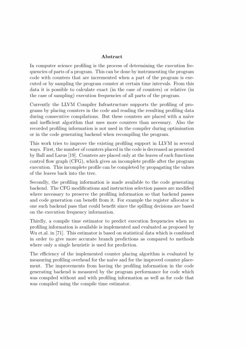


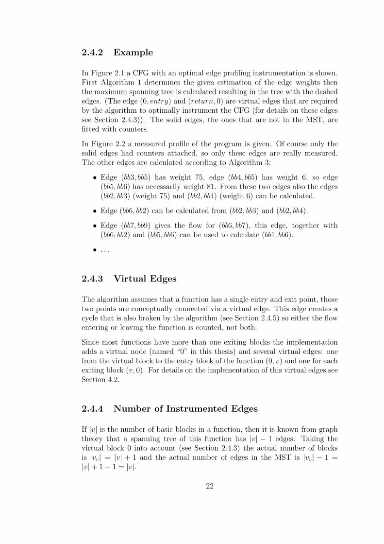
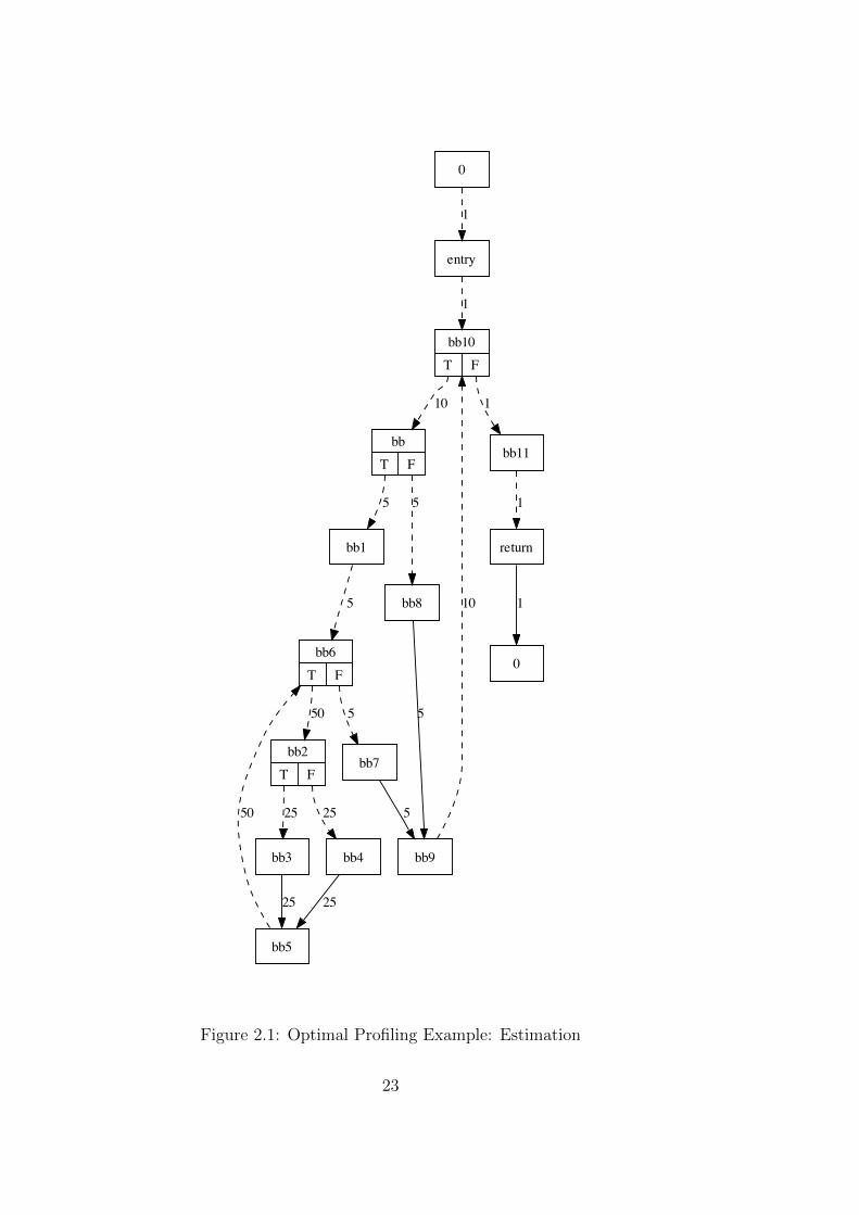
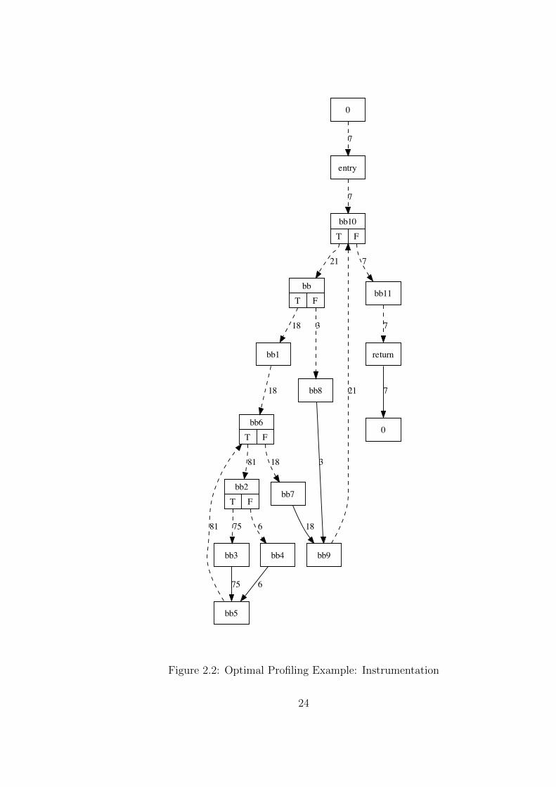


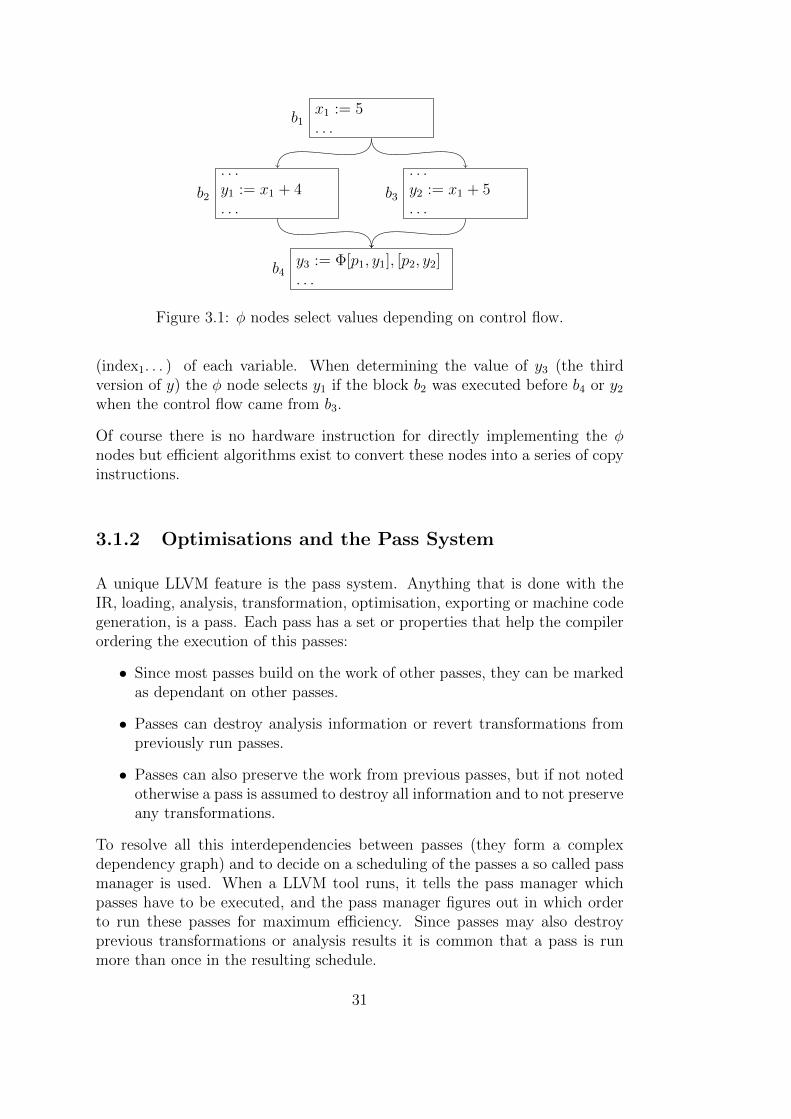
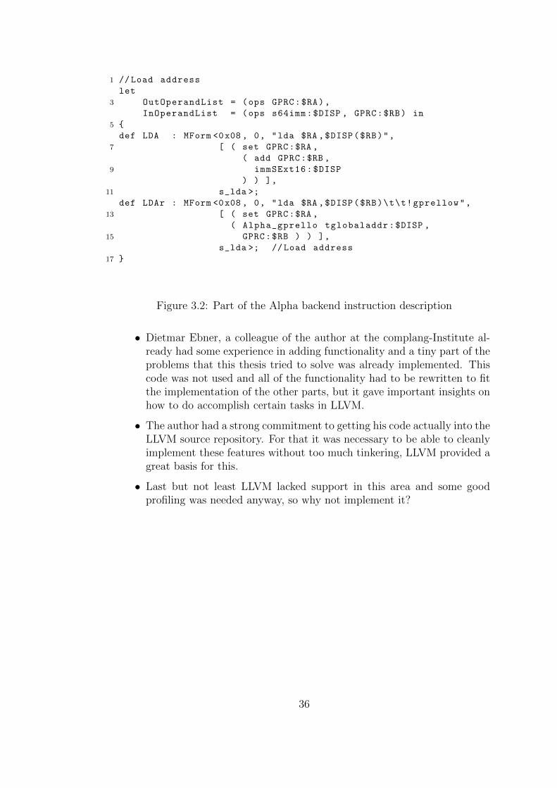
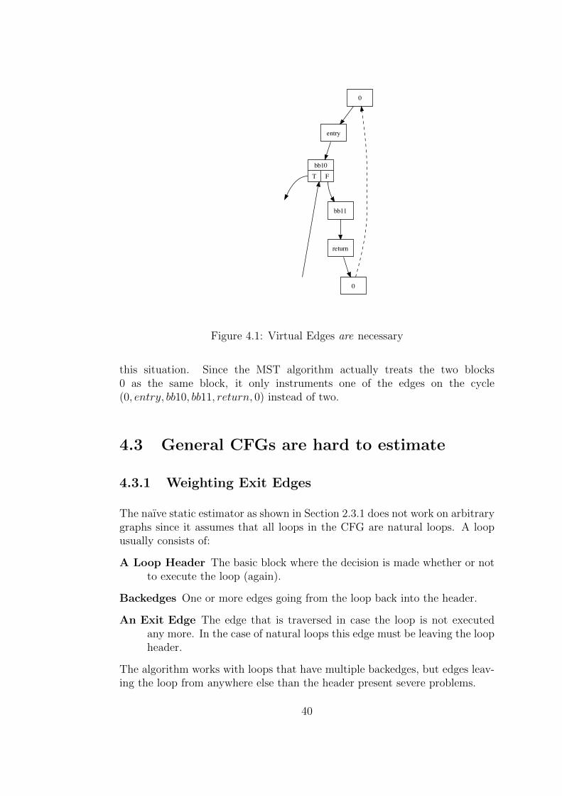
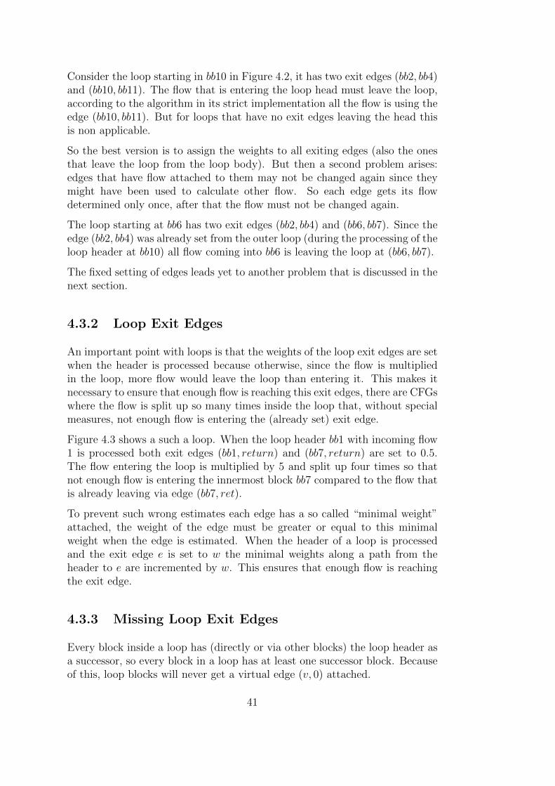
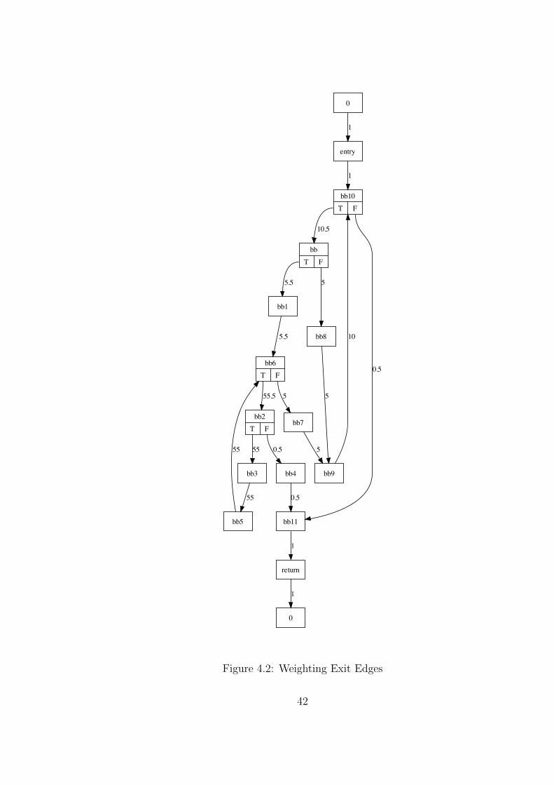
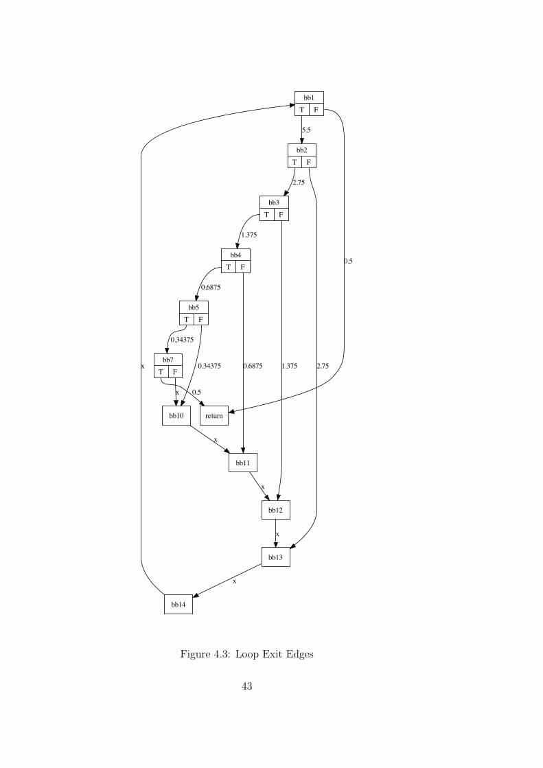
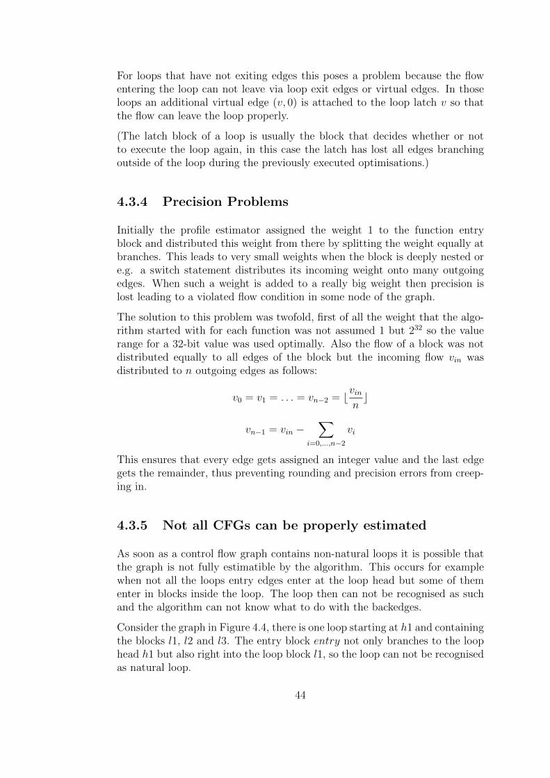
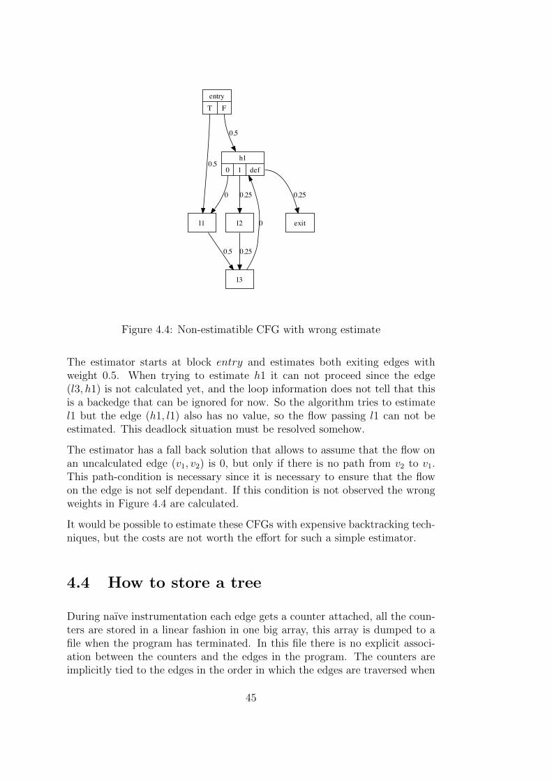

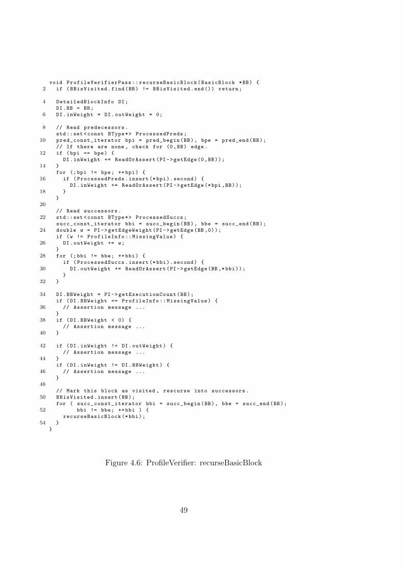

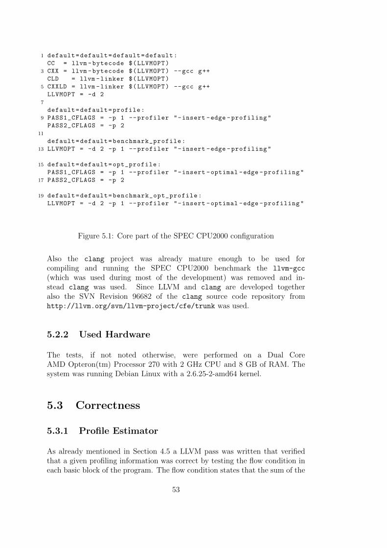
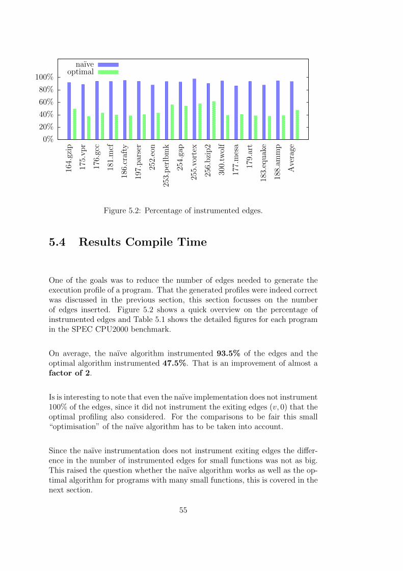
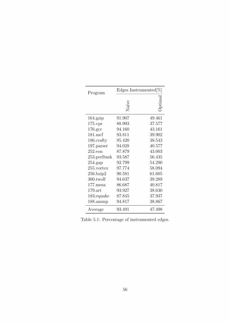
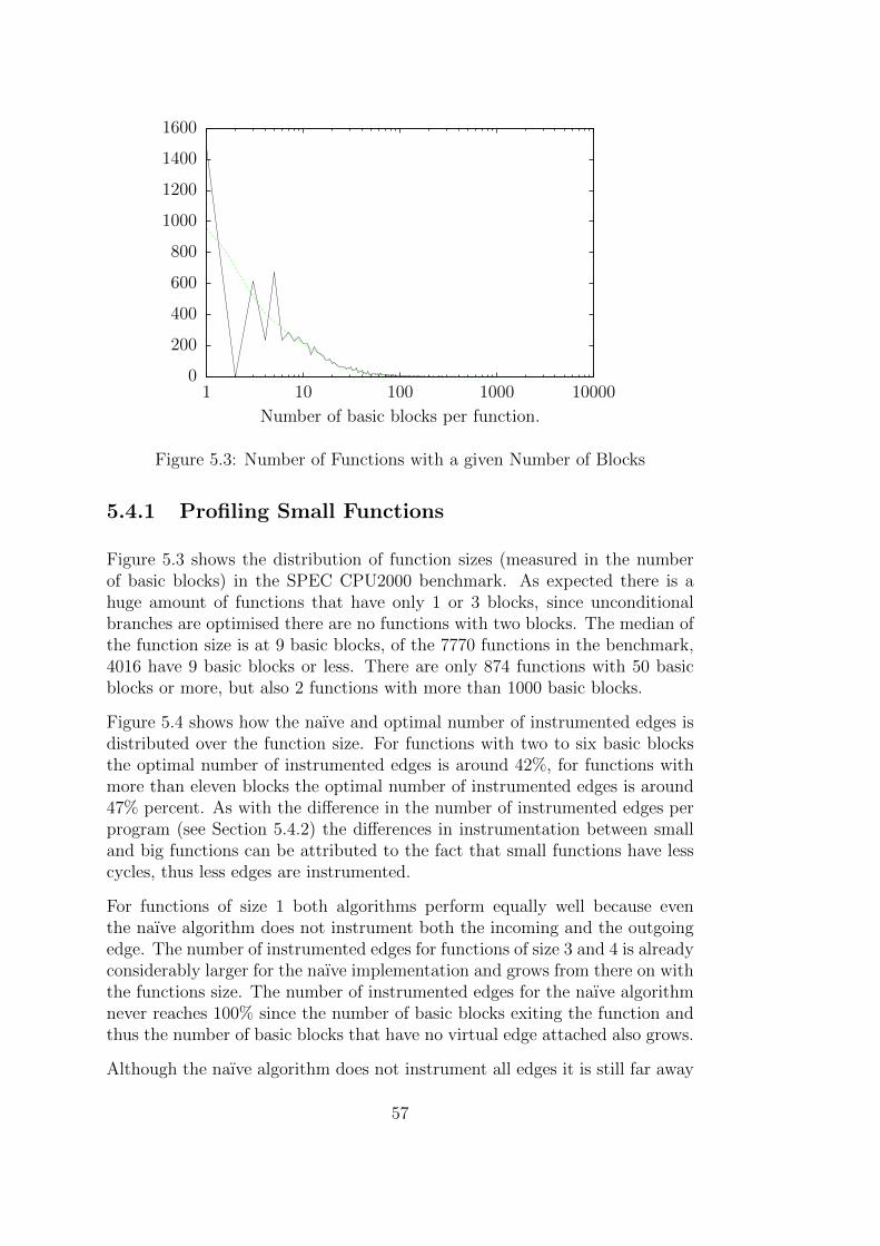
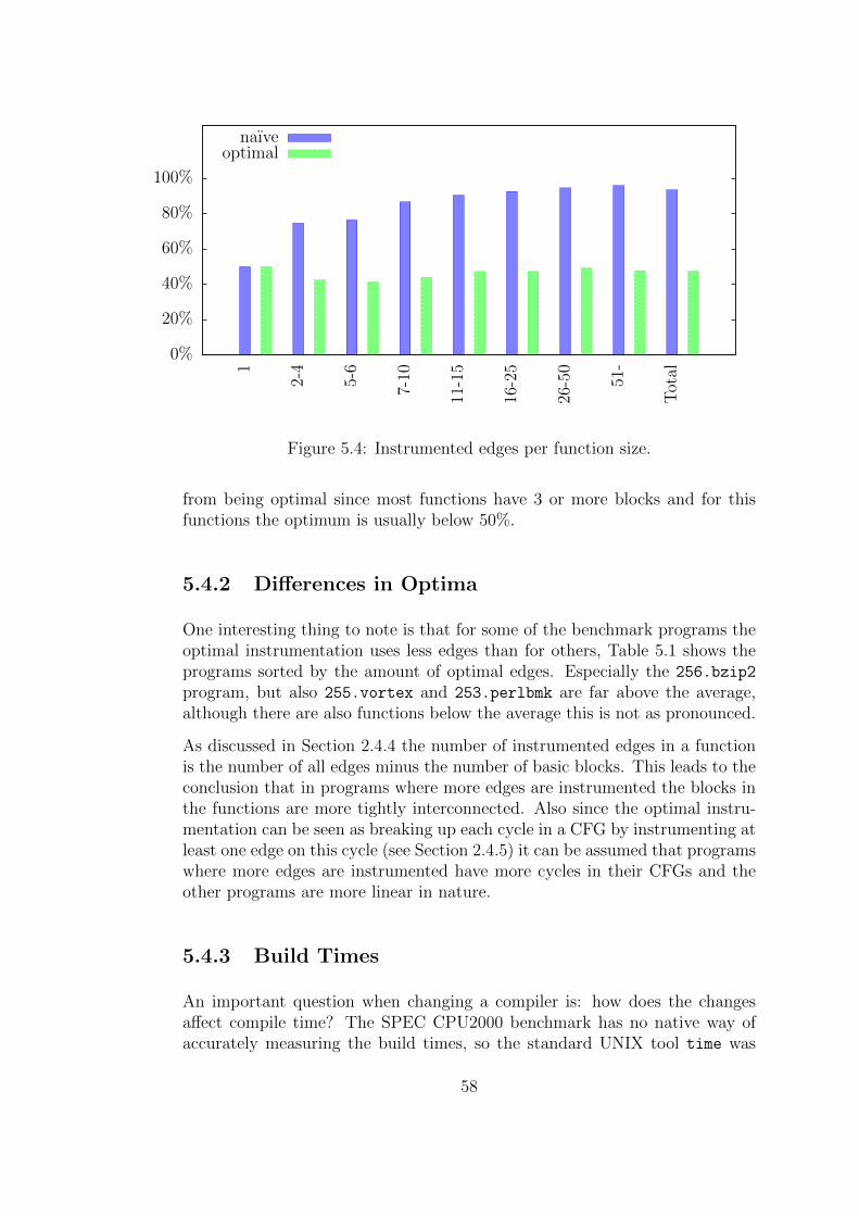
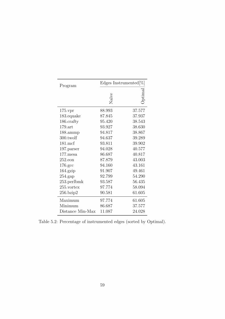
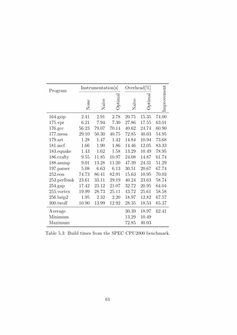
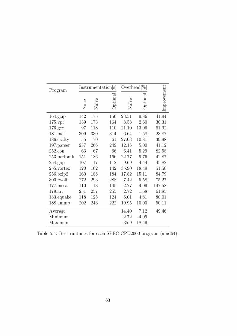
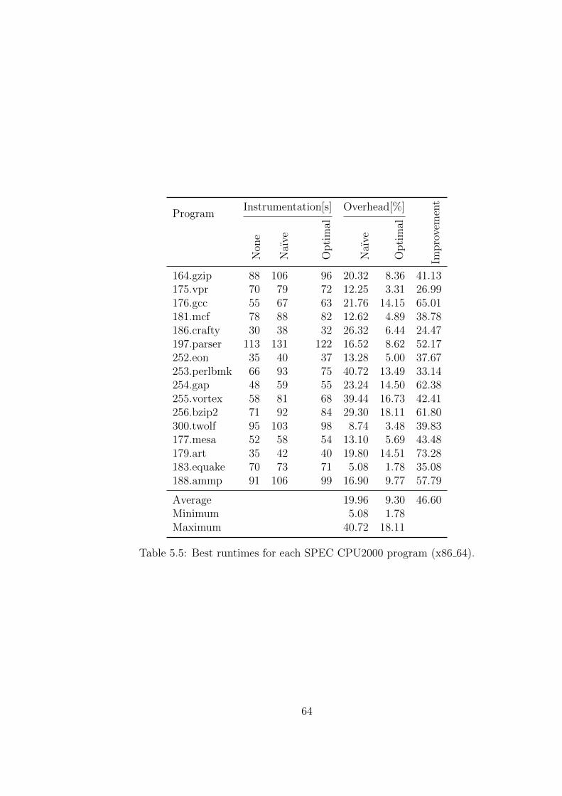
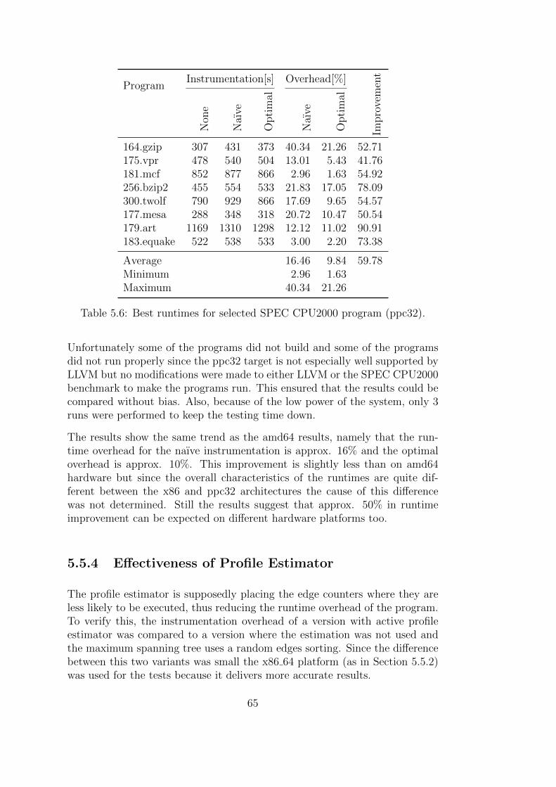
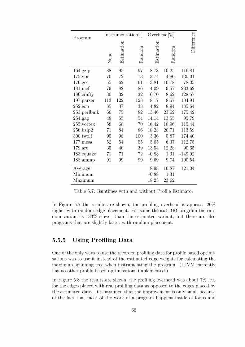
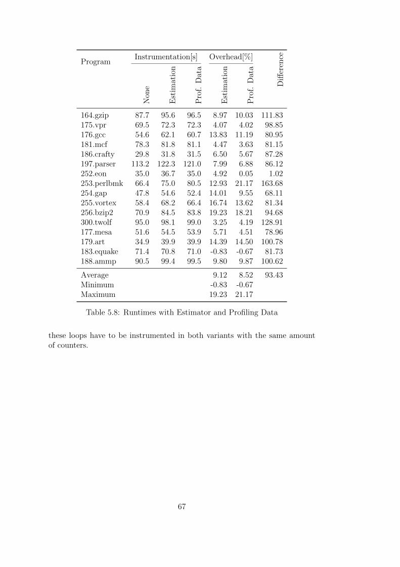


![Vorlesung Compiler für Eingebettete Systeme (SS14) · Compiler für Eingebettete Systeme [CS7506] Sommersemester 2014 Heiko Falk Institut für Eingebettete Systeme/Echtzeitsysteme](https://static.unterlagen.site/doc/80x56/5e0bcca2238c66363403635c/vorlesung-compiler-fr-eingebettete-systeme-ss14-compiler-fr-eingebettete-systeme.jpg)


