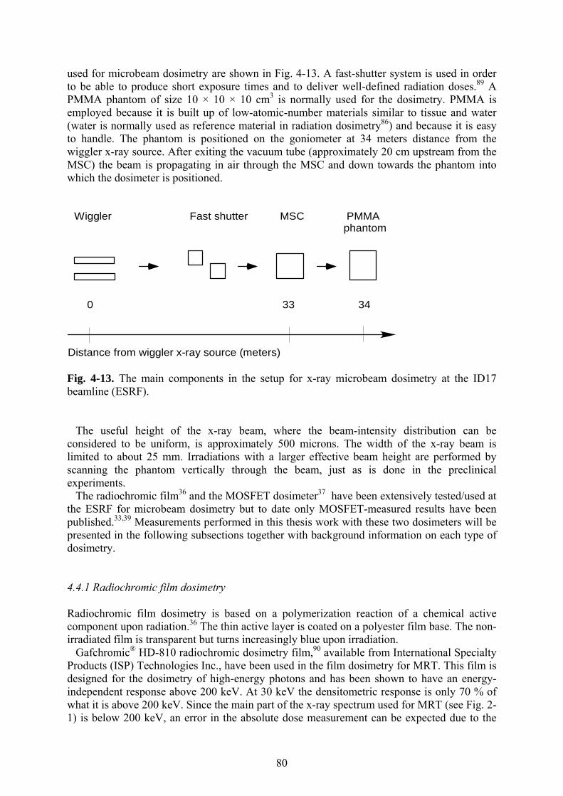
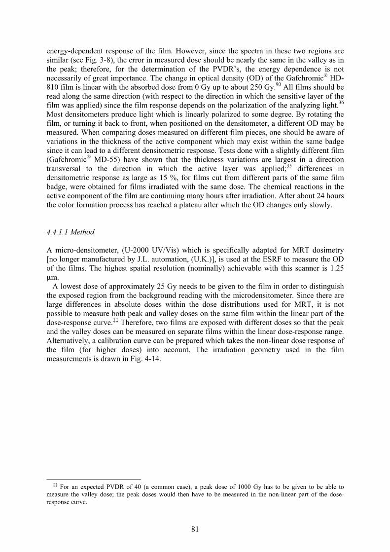
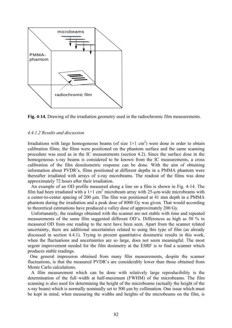
European Synchrotron Radiation Facility Dosimetry for synchrotron x-ray microbeam radiation therapy Erik Albert Siegbahn Vollständiger Abdruck der von der Fakultät für Physik der Technischen Universität München zur Erlangung des akademischen Grades eines Doktors der Naturwissenschaften genehmigten Dissertation. Vorsitzender: Univ.-Prof. Dr. J. L. van Hemmen Prüfer der Dissertation: 1. Hon.-Prof. Dr. H. G. Paretzke 2. Univ.-Prof. Dr. R. Krücken Die Dissertation wurde am 13.06.2007 bei der Technischen Universität München eingereicht und durch die Fakultät für Physik am 05.10.2007 angenommen.
Transcript
European Synchrotron Radiation Facility
Dosimetry for synchrotron x-ray
microbeam radiation therapy
Erik Albert Siegbahn
Vollständiger Abdruck der von der Fakultät für Physik der Technischen Universität München zur Erlangung des akademischen Grades eines Doktors der Naturwissenschaften genehmigten Dissertation.
Vorsitzender: Univ.-Prof. Dr. J. L. van Hemmen
Prüfer der Dissertation:
1. Hon.-Prof. Dr. H. G. Paretzke 2. Univ.-Prof. Dr. R. Krücken
Die Dissertation wurde am 13.06.2007 bei der Technischen Universität München eingereicht und durch die Fakultät für Physik am 05.10.2007 angenommen.
2
3
CONTENTS
1. INTRODUCTION................................................................................................................ 5 1.1 SYNCHROTRON X-RAY MICROBEAM RADIATION THERAPY................................................. 5 1.2 THE ACCURATE DETERMINATION OF ABSORBED DOSES ..................................................... 7
1.2.1 Limits to experimental dosimetry for MRT ............................................................... 8 1.2.1.1 Dose measurements in large homogeneous fields .................................................................... 9 1.2.1.2 Dose measurements in microbeams .................................................................................... 9 1.2.1.3 X-ray spectrum determination........................................................................................... 9
1.2.2 Calculations of the absorbed radiation dose .......................................................... 10
2. INTERACTIONS OF RADIATION WITH MATTER ................................................ 11 2.1 X-RAY INTERACTIONS WITH MATTER RELEVANT FOR MRT............................................. 11
2.1.1 Coherent (Rayleigh) scattering ............................................................................... 13 2.1.2 Incoherent (Compton) scattering ............................................................................ 14 2.1.3 Photoelectric effect.................................................................................................. 14 2.1.4 Atomic relaxation .................................................................................................... 15 2.1.5 Attenuation of x-rays with depth in a medium......................................................... 16
2.2 SECONDARY ELECTRON INTERACTIONS WITH MATTER .................................................... 16 2.2.1 Elastic scattering:.................................................................................................... 16 2.2.2 Inelastic scattering: ................................................................................................. 18
2.3 QUANTITIES USED FOR DESCRIBING THE DEPOSITION OF RADIATION ENERGY.................. 19 2.3.1 Absorbed dose ......................................................................................................... 19 2.3.2 Kerma (Kinetic energy released in matter)............................................................. 20
3. MONTE CARLO SIMULATIONS OF DOSE DEPOSITION ................................... 21 3.1 THE PENELOPE MC CODE ............................................................................................ 21 3.2 SIMULATION GEOMETRY AND DETAILS............................................................................ 22 3.3 DEPTH-DOSE CURVES ...................................................................................................... 22 3.4 TRANSVERSAL DOSE PROFILES ........................................................................................ 24 3.5 SPECTRA AND ANGULAR DISTRIBUTIONS OF SECONDARY PARTICLES .............................. 25 3.6 THE RELATIVE IMPORTANCE OF DIFFERENT INTERACTION PROCESSES............................. 29 3.7 DIFFERENCES IN ABSORBED DOSE FOR DIFFERENT BEAM SIZES........................................ 30 3.8 COMPARISON WITH CALCULATED DOSE PROFILES FROM EARLIER STUDIES...................... 32 3.9 COMPOSITE DOSE DISTRIBUTIONS AND PVDR’S.............................................................. 34 3.10 COMPARISON OF ABSORBED DOSES CALCULATED WITH DIFFERENT MC CODES ............ 40
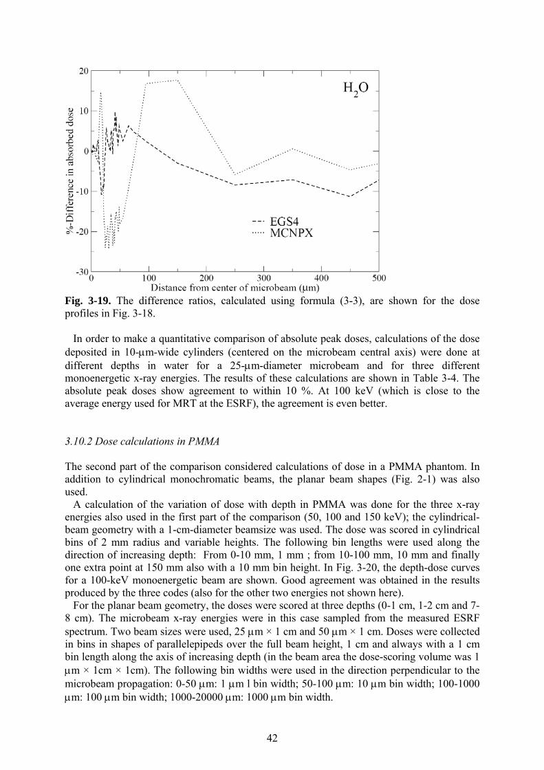
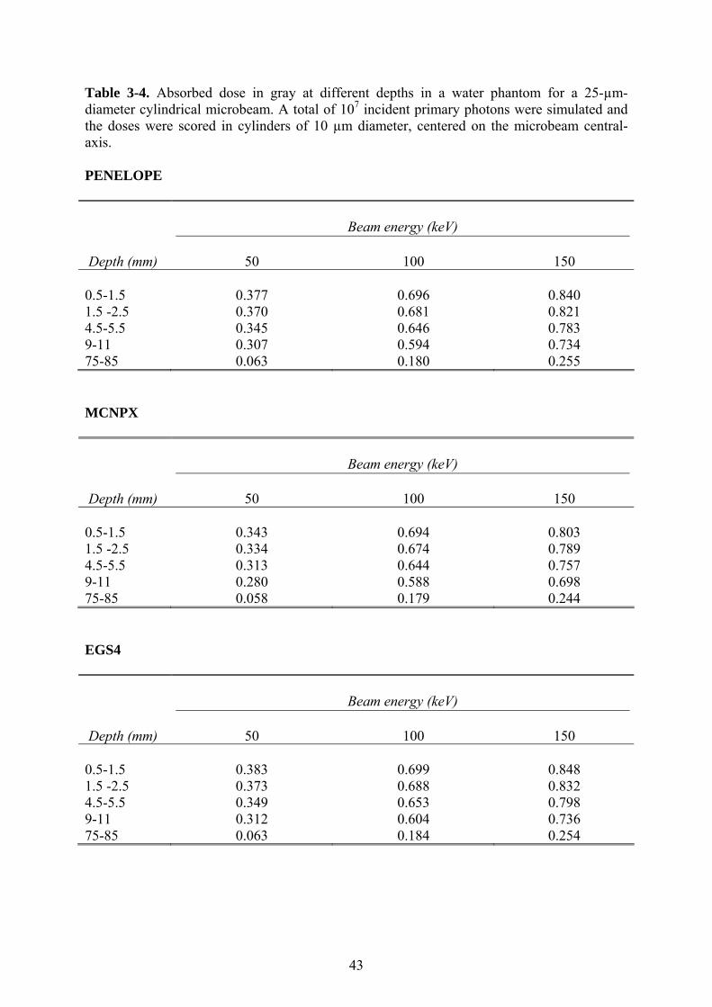
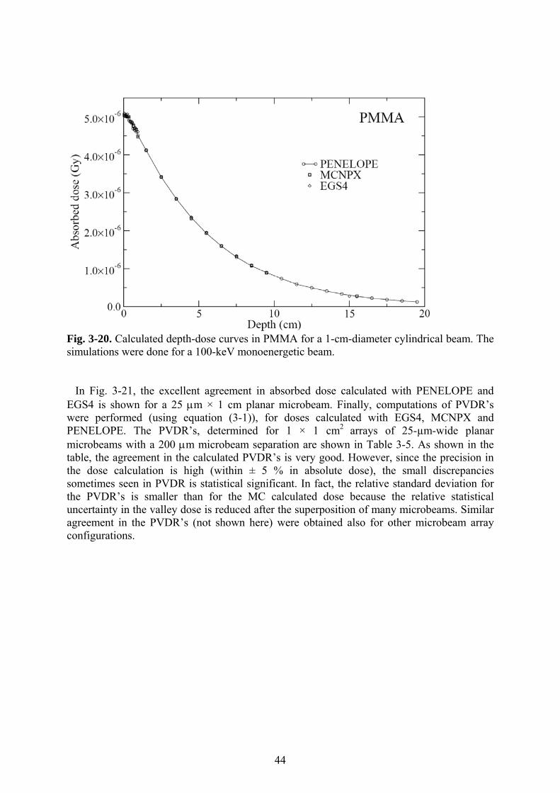
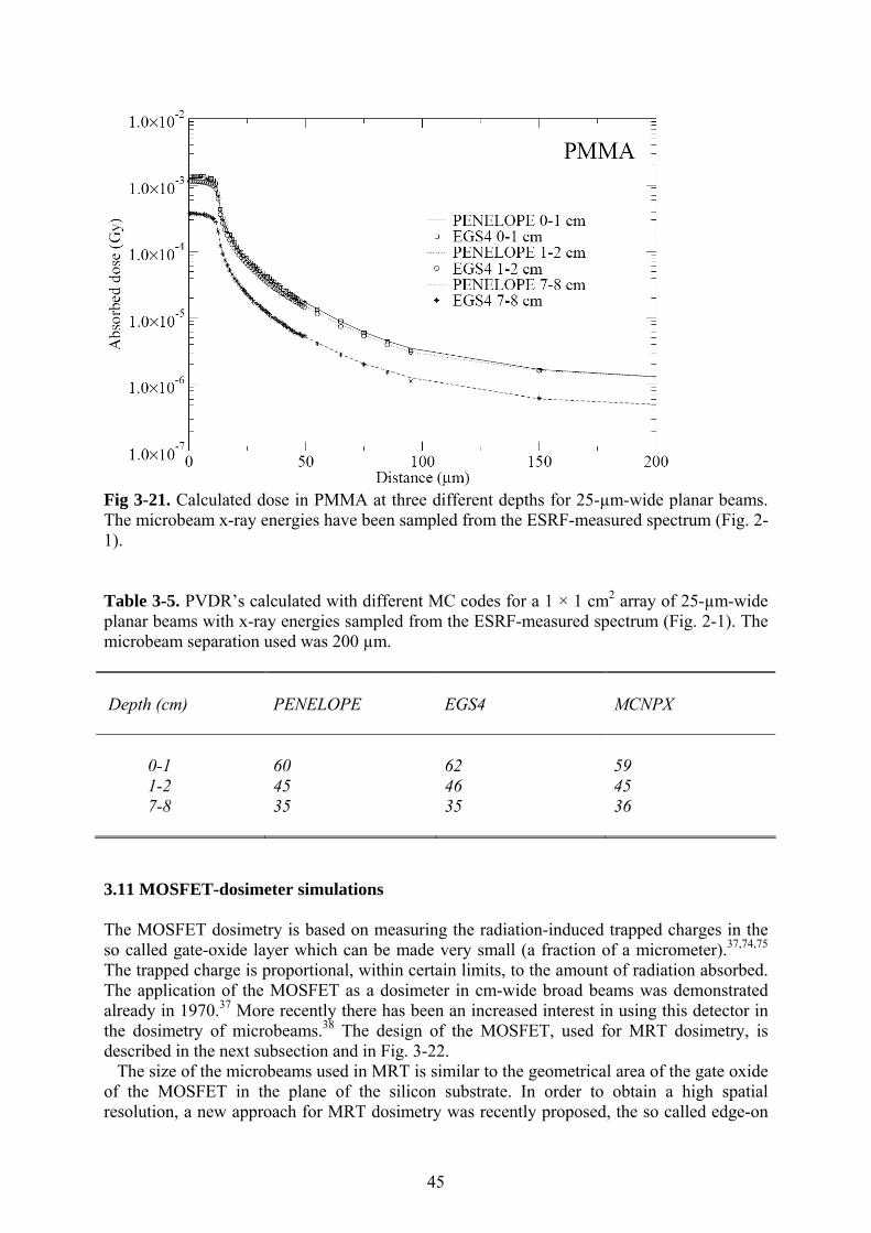
3.10.1 Dose calculations in water .................................................................................... 40 3.10.2 Dose calculations in PMMA ................................................................................. 42
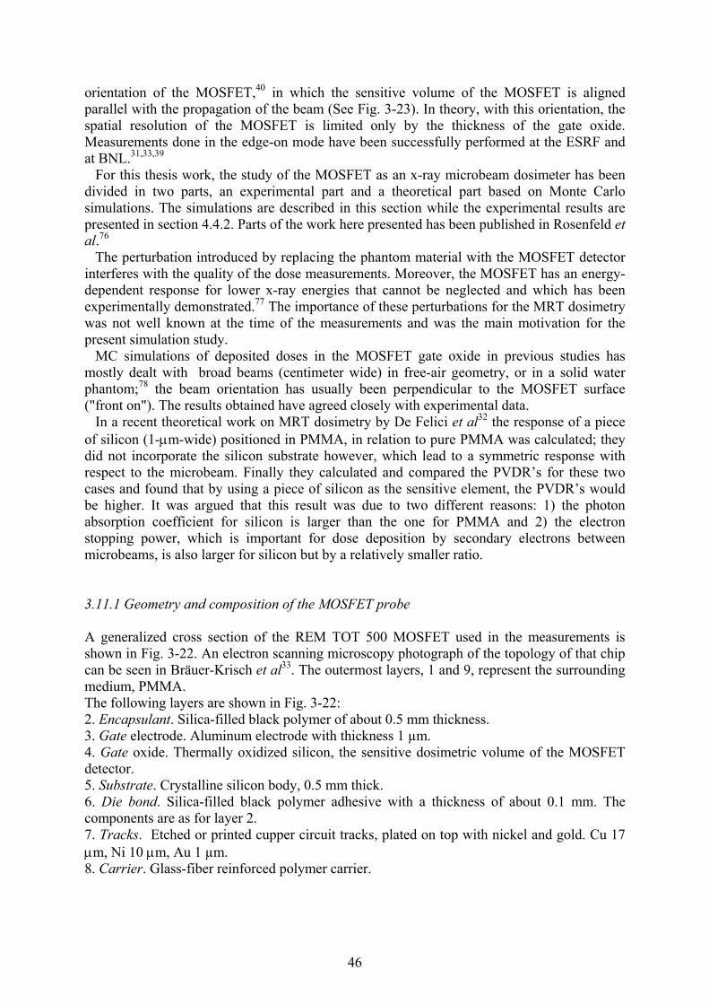
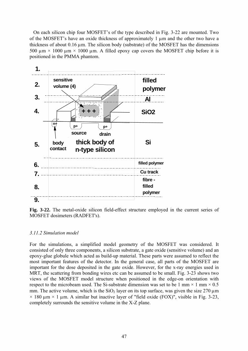
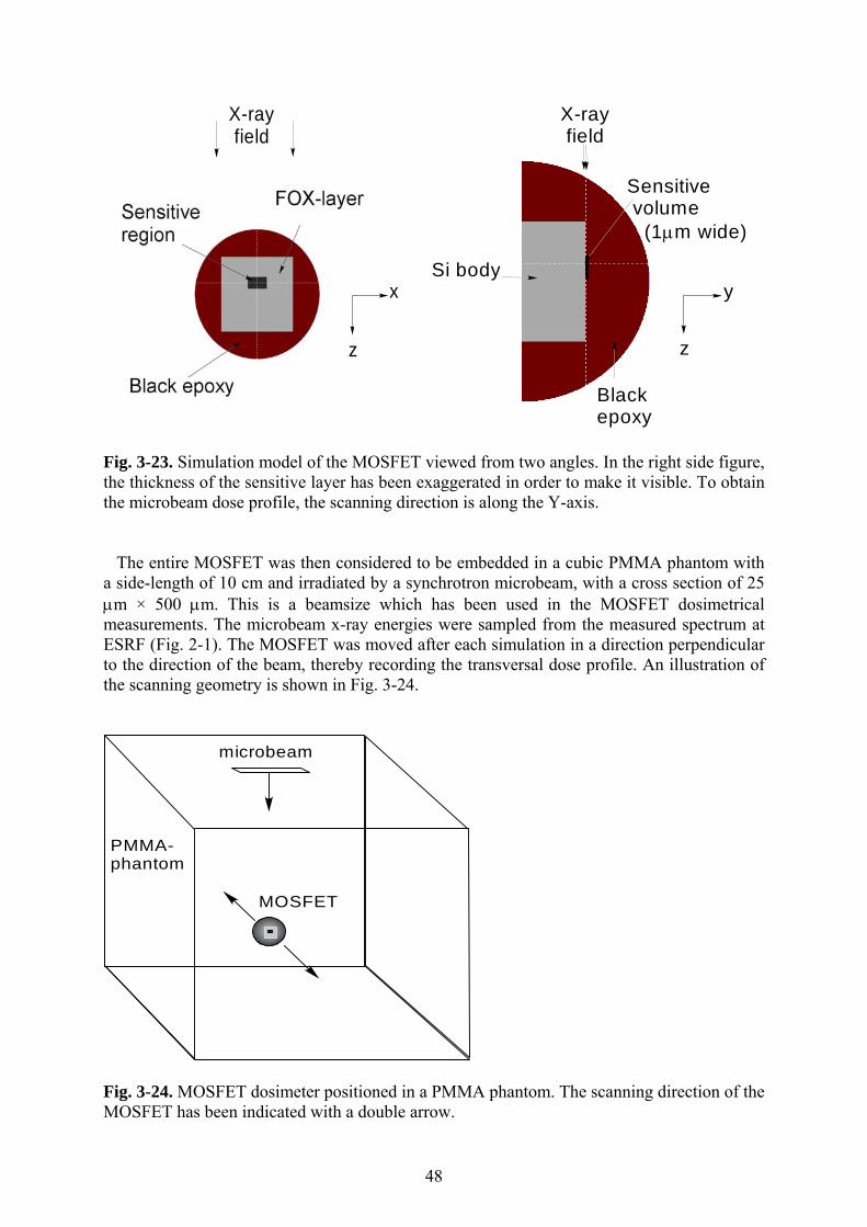
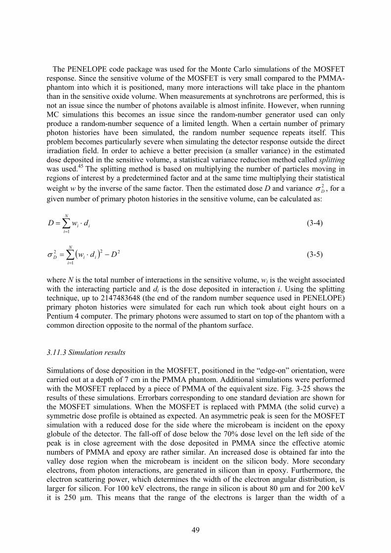
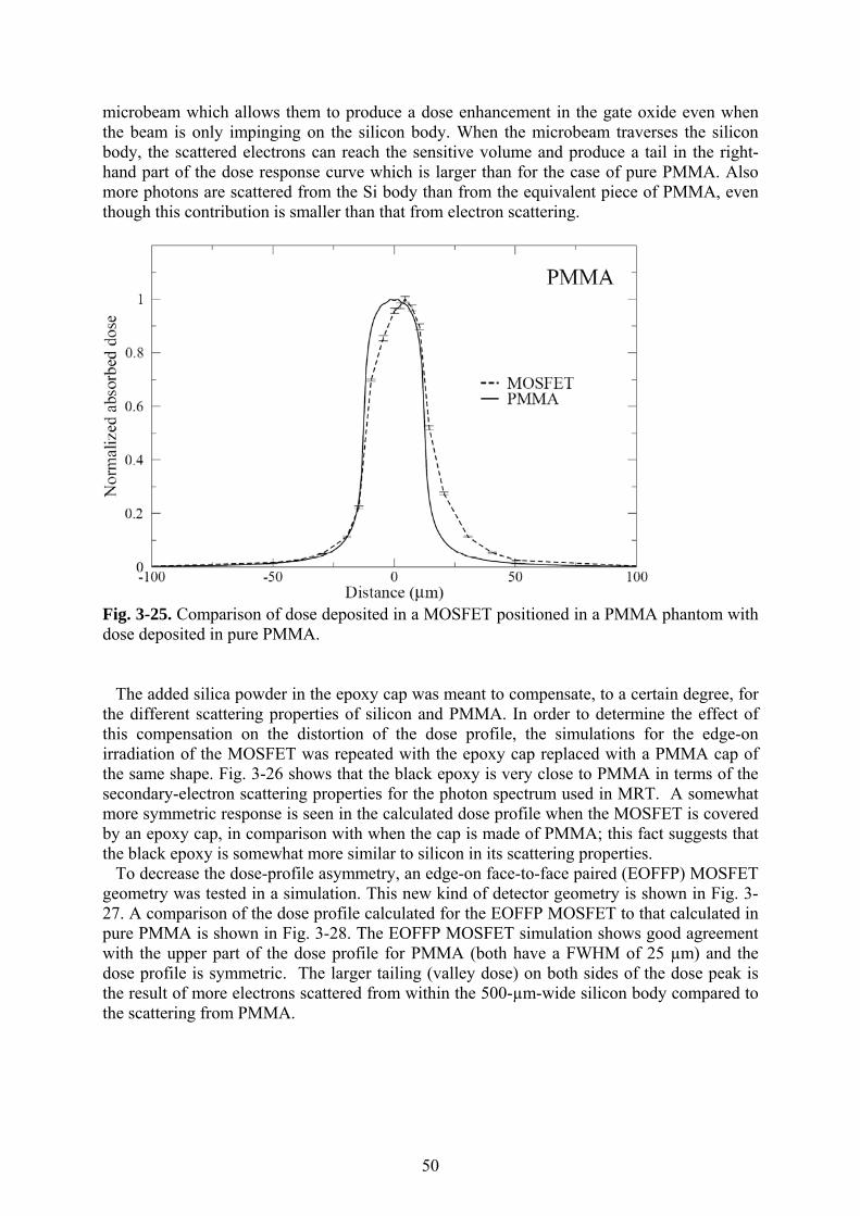
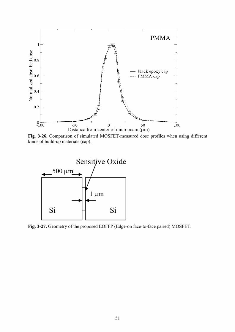
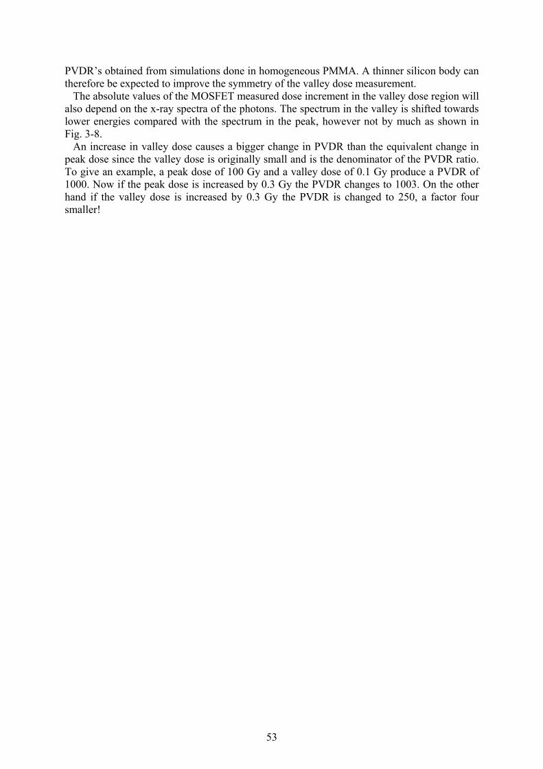
3.11 MOSFET-DOSIMETER SIMULATIONS............................................................................. 45 3.11.1 Geometry and composition of the MOSFET probe ............................................... 46 3.11.2 Simulation model................................................................................................... 47 3.11.3 Simulation results .................................................................................................. 49 3.11.4 Discussion ............................................................................................................. 52
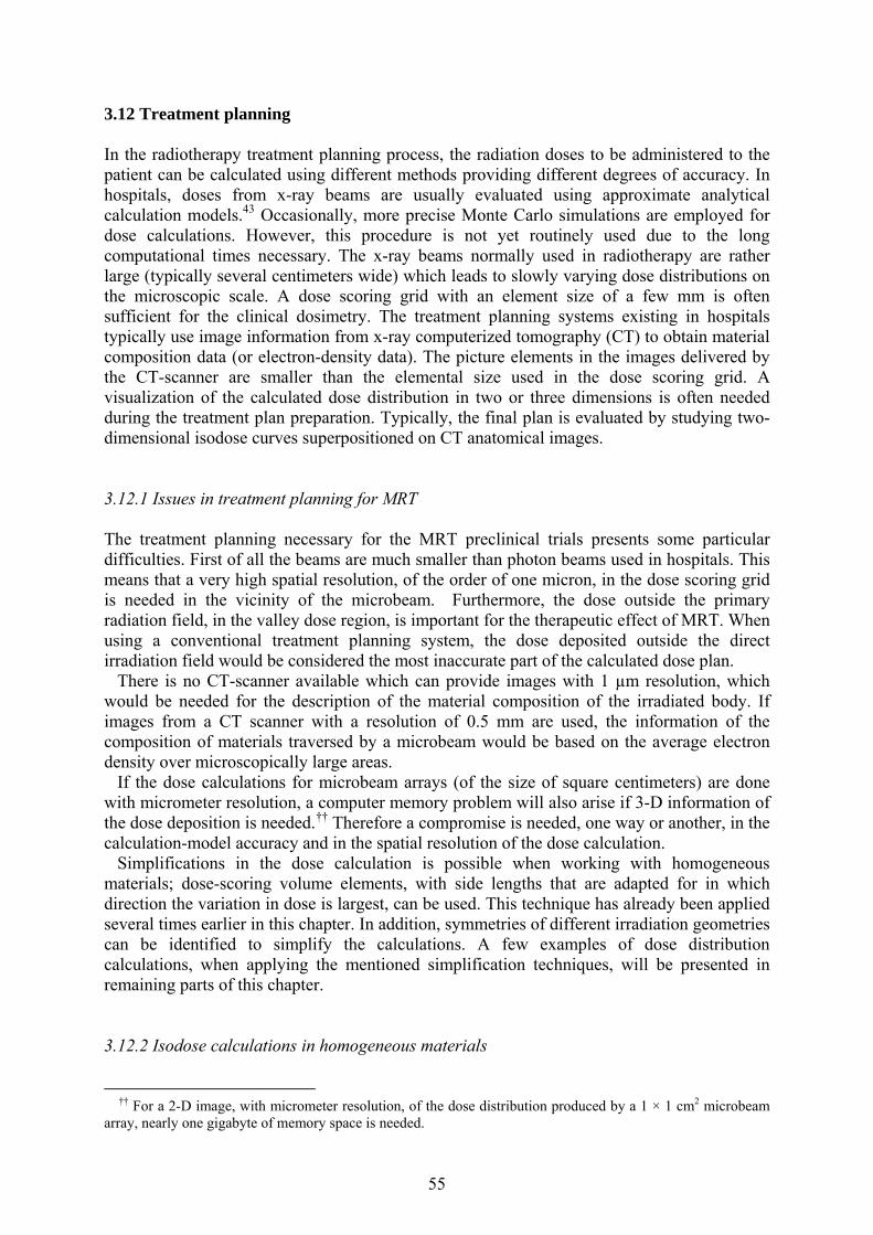
3.12 TREATMENT PLANNING.................................................................................................. 55 3.12.1 Issues in treatment planning for MRT................................................................... 55 3.12.2 Isodose calculations in homogeneous materials ................................................... 55
4
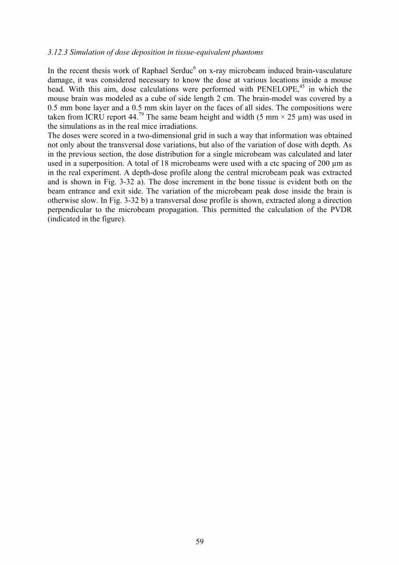
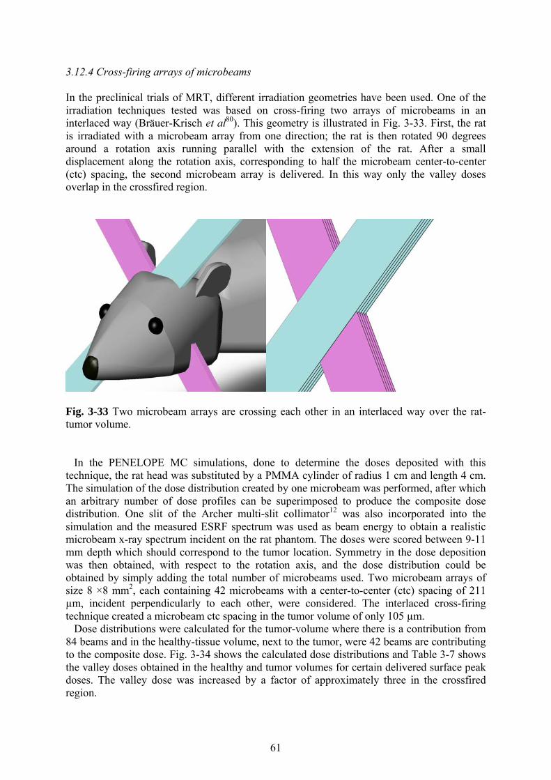
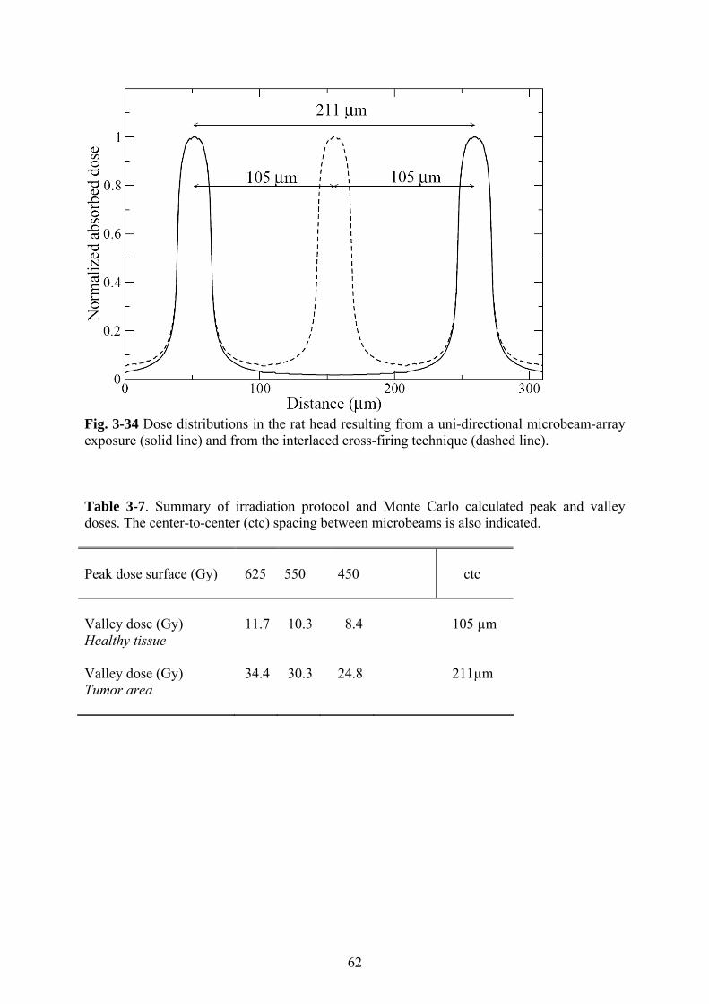
3.12.3 Simulation of dose deposition in tissue-equivalent phantoms............................... 59 3.12.4 Cross-firing arrays of microbeams ....................................................................... 61
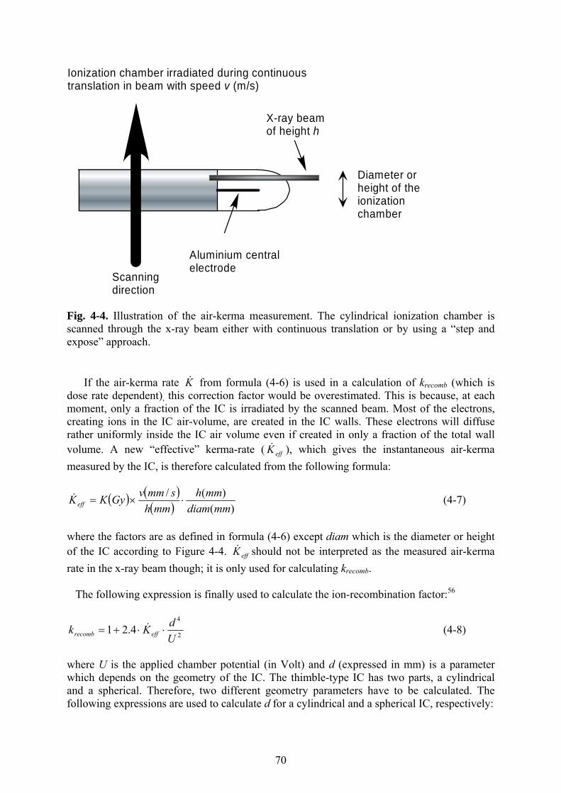
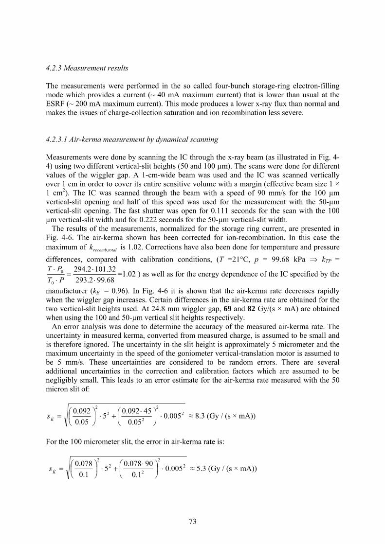
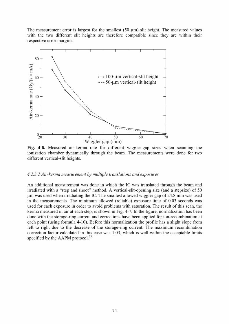
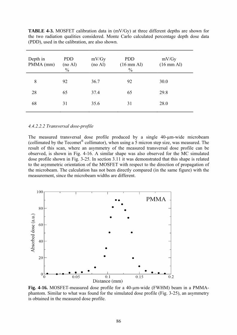
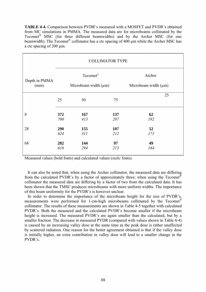
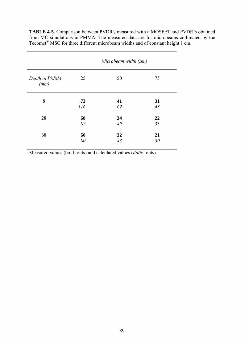
4.3.1 Multi-slit collimation of microbeams ...................................................................... 77 4.3.2 Measurements of the microbeam shapes................................................................. 78
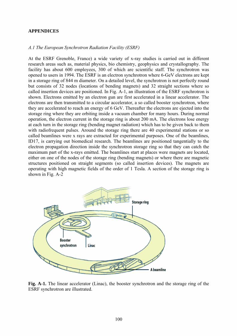
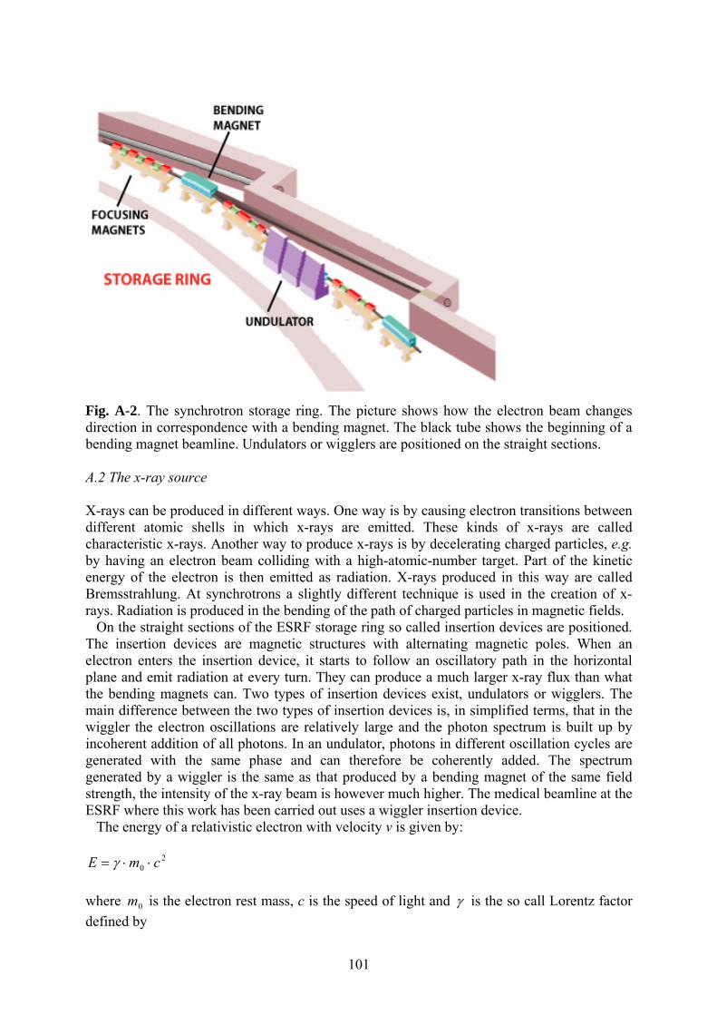
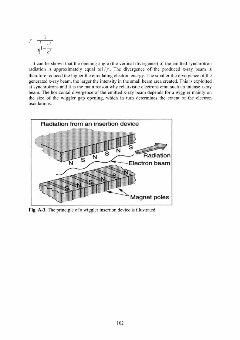
A.1 THE EUROPEAN SYNCHROTRON RADIATION FACILITY (ESRF) ......................................... 100 A.2 THE X-RAY SOURCE......................................................................................................... 101
5
1. INTRODUCTION 1.1 Synchrotron x-ray microbeam radiation therapy Irradiation of tumors with arrays of millimeter-wide x-ray beams was proposed 14 years after Röntgen's original discovery of x rays.1, 2a, 2b An unanticipated skin-sparing effect had been observed in animal experiments with this kind of irradiation geometry. Analogous techniques for spatially fractionated radiotherapy of cancer, using grids or sieves to produce the x-ray beam arrays, are still being used to date.3
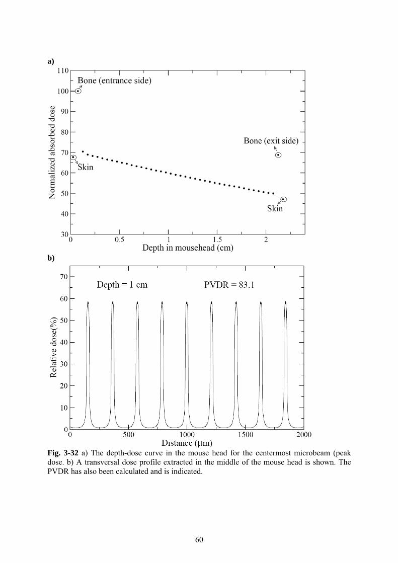
In the 1950s, at Brookhaven National Laboratory (BNL) (under the aegis of the USA NASA space exploration program), a deuteron microbeam was used to irradiate mice to simulate the damage in the human brain caused by energetic cosmic rays (e.g. a 60-GeV iron nucleus) from which astronauts could not be protected.4 Whereas the mouse-brain cortex in the path of the deuteron beam disappeared for relatively low doses delivered by a 1-mm-wide beam, it remained intact and apparently functional after it received five- to ten-fold higher doses from a 25-µm-wide microbeam of identical deuterons. Regeneration of damaged vasculature was believed to play a major role in the resistance of intensely irradiated mouse-brain tissue to cerebrocortical necrosis.5 Since nerve cells are consuming large amounts of sugar and oxygen the effect of a severed blood supply can be lethal. It was postulated (correctly, as it turned out in experiments performed half a century later6) that the vasculature in the microbeam path is rapidly repaired by nominally unirradiated endothelial cells near the track. On the other hand, when the tissue is irradiated with broad beams, the vessels and capillaries may be damaged over areas to large for effective repair to occur. A consensus as to the threshold beam width for failure of repair, if indeed there is a threshold width that applies to different normal tissues in various species, has not been reached.7 Later, experiments were done elsewhere to study the skin lesions produced by broad and micrometer-sized x-ray beams (produced by a conventional x-ray source).8 A skin-sparing effect was found, attributed to regeneration from surviving skin cells, when the irradiations were performed with the x-ray microbeam. Towards the end of the 20th century, 3rd-generation synchrotron light sources became available to the scientific community providing several orders of magnitude more intense x-ray beams than had been available earlier.9 Synchrotron radiation derives its name from a specific type of particle accelerator where it was produced for the first time.10 It is nowadays used to indicate radiation of a wide range of energies, from infrared to “hard” x-rays, emitted by charged particles moving at relativistic speeds in magnetic fields. In the beginning of the last decade, researchers at BNL started to use these new high-flux x-ray beams to study different phenomena in imaging and radiobiology.11 In the initial intents to perform µCT imaging of the head of an anaesthetized mouse, an unusually high normal-tissue resistance to high doses (~200 Gy), delivered by a microbeam of synchrotron-generated X-rays, was observed.† In fact, the trace of the microbeam had disappeared at the time of histopathological analysis. Based on these findings, it was proposed to treat tumors with an array of microbeams.12 By cross-firing the targeted cancer from several directions a considerable radiation dose could be delivered to volumes in which the microbeam arrays intersect. It was anticipated that such microbeam radiation therapy (MRT) might have relatively few adverse side-effects, thanks to the high tolerance of normal tissues to the x-ray microbeams.13 It was held that MRT could be especially useful for treating brain tumors in children, since the risks of delayed radiation damage are more serious in children than in
† Daniel Slatkin, personal communication, 2006
6
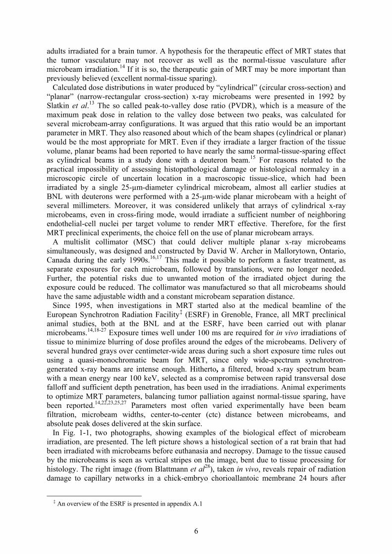
adults irradiated for a brain tumor. A hypothesis for the therapeutic effect of MRT states that the tumor vasculature may not recover as well as the normal-tissue vasculature after microbeam irradiation.14 If it is so, the therapeutic gain of MRT may be more important than previously believed (excellent normal-tissue sparing). Calculated dose distributions in water produced by “cylindrical” (circular cross-section) and “planar” (narrow-rectangular cross-section) x-ray microbeams were presented in 1992 by Slatkin et al.13 The so called peak-to-valley dose ratio (PVDR), which is a measure of the maximum peak dose in relation to the valley dose between two peaks, was calculated for several microbeam-array configurations. It was argued that this ratio would be an important parameter in MRT. They also reasoned about which of the beam shapes (cylindrical or planar) would be the most appropriate for MRT. Even if they irradiate a larger fraction of the tissue volume, planar beams had been reported to have nearly the same normal-tissue-sparing effect as cylindrical beams in a study done with a deuteron beam.15 For reasons related to the practical impossibility of assessing histopathological damage or histological normalcy in a microscopic circle of uncertain location in a macroscopic tissue-slice, which had been irradiated by a single 25-µm-diameter cylindrical microbeam, almost all earlier studies at BNL with deuterons were performed with a 25-µm-wide planar microbeam with a height of several millimeters. Moreover, it was considered unlikely that arrays of cylindrical x-ray microbeams, even in cross-firing mode, would irradiate a sufficient number of neighboring endothelial-cell nuclei per target volume to render MRT effective. Therefore, for the first MRT preclinical experiments, the choice fell on the use of planar microbeam arrays. A multislit collimator (MSC) that could deliver multiple planar x-ray microbeams simultaneously, was designed and constructed by David W. Archer in Mallorytown, Ontario, Canada during the early 1990s.16,17 This made it possible to perform a faster treatment, as separate exposures for each microbeam, followed by translations, were no longer needed. Further, the potential risks due to unwanted motion of the irradiated object during the exposure could be reduced. The collimator was manufactured so that all microbeams should have the same adjustable width and a constant microbeam separation distance. Since 1995, when investigations in MRT started also at the medical beamline of the European Synchrotron Radiation Facility‡ (ESRF) in Grenoble, France, all MRT preclinical animal studies, both at the BNL and at the ESRF, have been carried out with planar microbeams.14,18-27 Exposure times well under 100 ms are required for in vivo irradiations of tissue to minimize blurring of dose profiles around the edges of the microbeams. Delivery of several hundred grays over centimeter-wide areas during such a short exposure time rules out using a quasi-monochromatic beam for MRT, since only wide-spectrum synchrotron-generated x-ray beams are intense enough. Hitherto, a filtered, broad x-ray spectrum beam with a mean energy near 100 keV, selected as a compromise between rapid transversal dose falloff and sufficient depth penetration, has been used in the irradiations. Animal experiments to optimize MRT parameters, balancing tumor palliation against normal-tissue sparing, have been reported.14,22,23,25,27 Parameters most often varied experimentally have been beam filtration, microbeam widths, center-to-center (ctc) distance between microbeams, and absolute peak doses delivered at the skin surface. In Fig. 1-1, two photographs, showing examples of the biological effect of microbeam irradiation, are presented. The left picture shows a histological section of a rat brain that had been irradiated with microbeams before euthanasia and necropsy. Damage to the tissue caused by the microbeams is seen as vertical stripes on the image, bent due to tissue processing for histology. The right image (from Blattmann et al28), taken in vivo, reveals repair of radiation damage to capillary networks in a chick-embryo chorioallantoic membrane 24 hours after
‡ An overview of the ESRF is presented in appendix A.1
7
microbeam irradiation. The embryo (which was not irradiated), the yolk and the chorioallantoic membrane were separated from the egg shell six days before the irradiation and were maintained alive in a Petrie dish; later this permitted to study the radiation damage and the repair thereof in vivo with a microscope. Some repair of radiation damage is depicted by neovascular anastomoses [communication between blood vessels by means of collateral channels (indicated by parallel arrows)] between intact capillary networks, bridging parallel columns of tissue previously containing identical intact capillary networks that had been ablated by the microbeams.
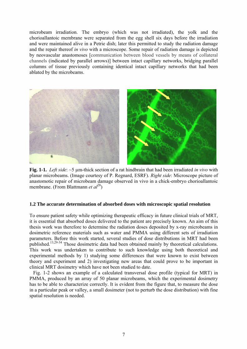
Fig. 1-1. Left side: ~5 µm-thick section of a rat hindbrain that had been irradiated in vivo with planar microbeams. (Image courtesy of P. Regnard, ESRF). Right side: Microscope picture of anastomotic repair of microbeam damage observed in vivo in a chick-embryo chorioallantoic membrane. (From Blattmann et al28) 1.2 The accurate determination of absorbed doses with microscopic spatial resolution To ensure patient safety while optimizing therapeutic efficacy in future clinical trials of MRT, it is essential that absorbed doses delivered to the patient are precisely known. An aim of this thesis work was therefore to determine the radiation doses deposited by x-ray microbeams in dosimetric reference materials such as water and PMMA using different sets of irradiation parameters. Before this work started, several studies of dose distributions in MRT had been published.13,29-34 Those dosimetric data had been obtained mainly by theoretical calculations. This work was undertaken to contribute to such knowledge using both theoretical and experimental methods by 1) studying some differences that were known to exist between theory and experiment and 2) investigating new areas that could prove to be important in clinical MRT dosimetry which have not been studied to date. Fig. 1-2 shows an example of a calculated transversal dose profile (typical for MRT) in PMMA, produced by an array of 50 planar microbeams, which the experimental dosimetry has to be able to characterize correctly. It is evident from the figure that, to measure the dose in a particular peak or valley, a small dosimeter (not to perturb the dose distribution) with fine spatial resolution is needed.
8
Fig. 1-2. Transversal dose profile in PMMA, obtained from MC simulations, produced by an array of x-ray microbeams, as used for MRT. The positions of the centermost peak and valley doses have been indicated. Theoretical dosimetry is necessary for the practical development of MRT and it is especially important that it is benchmarked against experimental dosimetry. An important advantage of computational dosimetry is that doses inside animals and humans, where it is difficult (or impossible) to perform measurements, can be calculated. The influence on the dose distribution of various combinations of irradiation parameters can be computed and compared, so that treatment plans for deep-seated lesions may be optimized in silico (via computer simulations). 1.2.1 Limits to experimental dosimetry for MRT The determination of doses from x-ray microbeams is demanding for several reasons. First, the size of the microbeams makes it difficult to find a detector small enough to be able to characterize the dose variations correctly. Second, the x-ray energies involved are relatively low (compared with photon energies used in hospital, linear-accelerator (LINAC) based radiotherapy) which makes the choice of detector material important. In fact, the dose-energy non-linearity of certain solid-state detectors can become an issue. Furthermore, the beam used for MRT is unique in the sense that it is extremely intense which can cause saturation in the detected signal. This fact limits the available instruments and techniques which can be used for measurements. There is no commercial dosimeter system available that can completely characterize the dose deposition with a resolution that meets the needs of MRT. Instead, the dosimetry has to rely on a combination of different experimental methods. The experimental dosimetry for MRT can be divided into two parts: 1) dose measurements in large homogeneous fields. 2) dose measurements in microbeams. In addition a measurement of the x-ray spectrum needs to be done since it is of importance for both the experimental dosimetry (to select suitable
9
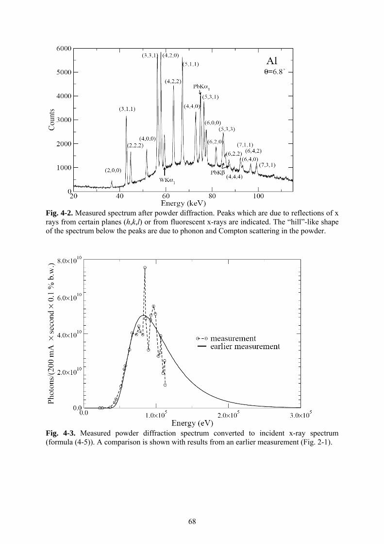
detectors) and for the theoretical dosimetry (to obtain the initial beam spectrum used in the dose calculations). Each experimental part will be briefly introduced in the following subsections. Measurements done within the frame of this thesis work will be presented in chapter 4. 1.2.1.1 Dose measurements in large homogeneous fields At the ESRF, for the absolute dose determination in large (1 × 1 cm2) fields, ionization chambers (IC’s) are used. Recommendations in well-established protocols for x-ray beam dosimetry are followed.35 The uncollimated x-ray flux is too high for the ionization chambers available which results in charge-collection saturation. Therefore the beam is strongly collimated to reduce the flux while the IC is rapidly scanned through the beam. The scanning is also necessary since the synchrotron beam has a “laminar” shape, i.e. it is wide in the horizontal plane but it is narrow (less than 1 mm) in the vertical direction, whereas the IC used has been calibrated at a standard laboratory in a wide beam. To reduce the difficulties in the absolute dose measurements related to the high photon flux, the experimental data can be acquired when the synchrotron storage ring is running at low electron current; the dosimetric results can then be linearly scaled with this current. Nevertheless it is considered necessary for the MRT application to be able to make absolute dose measurements under exactly the same condition, i.e. the same storage-ring current that is used in the preclinical trials; only then can the dose be controlled just before a treatment. 1.2.1.2 Dose measurements in microbeams For the x-ray microbeams (typical size: 25 μm × 500 μm), dosimetry is performed in a polymetyl methacralate (PMMA) phantom. Radiochromic films36 and metal-oxide semi-conducting field-effect transistors37-40 (MOSFET’s) have been tested as microbeam dosimeters. The radiochromic-film measurements provide important information about dose gradients and give a 2-D picture of the dose deposition, but do not provide a sufficiently accurate absolute dosimetry for MRT. The MOSFET dosimeter used at the ESRF is being developed specifically for the MRT program.33,39 The highest resolution is obtained when the extension of the sensitive volume of the MOSFET is parallel with the propagation of the beam; this orientation is called the edge-on orientation.40 The feasibility of performing dosimetric measurements for MRT with this irradiation geometry has been demonstrated.31,33 In this orientation the resolution of the MOSFET is determined by the thickness of its sensitive layer which is less than a micrometer. The perturbation on the dose measurement caused by the MOSFET detector itself remains to be determined. 1.2.1.3 X-ray spectrum determination It is not possible to make a direct spectrum measurement using standard procedures (by putting a semi-conducting detector in the direct beam) since the detector would be destroyed by the intense beam. X-ray spectrum measurements at the medical beamline are performed by using a technique called x-ray powder diffraction.9 The photon intensity scattered from the micro-crystalline powder is many orders of magnitude smaller than the primary-beam intensity and will therefore not saturate the detector. By measuring the spectrum and intensity
10
of x-rays diffracted into a selected solid angle, the x-ray spectrum incident on the powder can be reconstructed. 1.2.2 Calculations of the absorbed radiation dose Using Monte Carlo (MC) simulations the dosimetrical quantities relevant for MRT can be calculated. Radiation transport calculations with the MC method are based on following each particle in a beam, through each collision and deflection, until it is absorbed. Particles are transported from one interaction point to the next one along straight paths. At the collision points, so called secondary particles, normally electrons but occasionally photons (Brems-strahlung or fluorescence photons), can be created. The trajectories of the secondary particles can be simulated after the primary particle has been absorbed. This approach can be used in amorphous (non-crystalline) materials where interference effects from particle waves scattered from different atoms are negligible. The MC method has been used for several decades in different areas of physics and the first MC simulation of radiation shower production (known to the author) was performed by Wilson in the year 1952.41 A historical review, by Rogers et al,42 on the use of MC methods in medical physics applications has recently been published. The main advantage of the MC method is that deflection angles and energy losses can be simulated using the probability distributions calculated with the most accurate physical interaction models. Any analytical dose calculation necessarily makes use of several approximations in the physical models.43 The MC method is in principle only limited by the accuracy of the physical interaction model implemented in the code and the faithfulness of the geometry used as input in the simulation. A restriction on the usefulness of MC simulations for dosimetry is due to its statistical nature. A large number of primary photon histories may have to be simulated before the calculated dose distribution stabilizes, which is the reason why MC simulations are not routinely used in hospital clinics yet. Instead, approximate analytical formulas with which the dose can be rapidly evaluated are normally preferred.43 For MRT-MC dosimetry the computing times can be very long (up to several days) to obtain the necessary statistical precision. Detailed MC simulation of the radiation transport, from generation of x-rays in the synchrotron storage ring to the dose deposition in a small detector inside a phantom, is not feasible due to the extremely low efficiency of such a simulation. In earlier MRT studies, schemes have been developed to increase the computational efficiency.13,29-32 Moreover, in the MC simulations of dose deposition in MRT, the particles need to be followed down to energies which are lower than usual (in standard radiotherapy) because the resolution needed in the calculated dose distribution is on the micrometer scale. Several non-standard detectors used in MRT experimental dosimetry (e.g. the MOSFET) need to be characterized in order to be able to rely on their results and if necessary determine correction factors. This characterization can partly be done with MC simulations. Previously, the microbeam dose profiles and the PVDR’s have been determined with the MC codes EGS444 and PSI-GEANT3.30 There are some differences in the results obtained with these codes for the same irradiation parameters and dose-scoring geometry. In this work, the well-established MC-code PENELOPE45 has been used. This code has been widely used in medical physics applications.46-50 Since there are important differences in the physics and transport algorithms implemented in different MC codes, a comparison of dosimetric results (obtained with different codes) has been performed in this thesis work to validate the results.
11
2. INTERACTIONS OF RADIATION WITH MATTER In this chapter, different interactions will be described in terms of the differential scattering cross section, dσ/dΩ, defined as: 51
0
),(I
Idd φθσ
=Ω
(2-1)
where I0 = is the flux of particles (of a specific energy) incident on an atom and I(θ,φ) is the flux of scattered particles passing through the solid angle element dΩ=sinθ⋅dθ⋅dφ The total scattering cross section per atom, σ, is given by:
∫ Ω⋅Ω
= dddσσ (2-2)
The mean free path (for particles of a specific energy), λ, between interactions in a medium with N atoms per unit volume is given by:
σλ
⋅=
N1 (2-3)
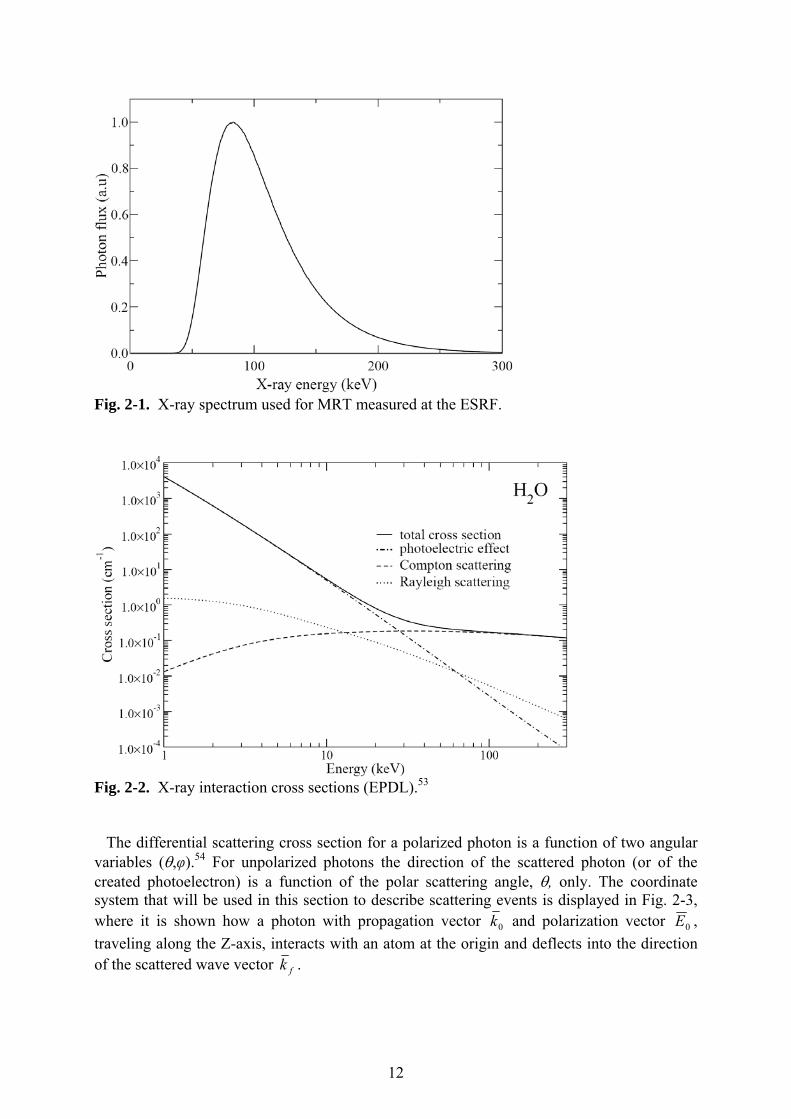
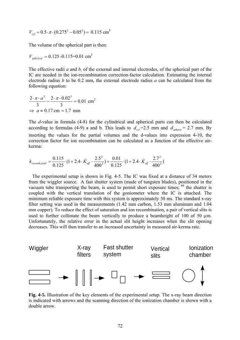
Later in this chapter, simple analytical cross sections will be presented with the aim of showing general dependencies, but they will not be used in this work in any calculation. More accurate cross sections exist for the interaction types described, though in tabulated form. The x-rays produced by the wiggler insertion device at the medical beamline are linearly polarized. Therefore, in section 2.1, x-ray interaction cross sections will be presented for linearly-polarized x-ray photons. However, the total cross section is the same for polarized and unpolarized photons, which means that the mean-free path between photon interactions is unaltered. In certain x-ray interactions (i.e. the photoelectric effect and Compton scattering), parts of the x-ray energy is transferred to an atomic electron which then is ejected from the atom. In section 2.2, a brief description of the secondary-electron interactions is presented. Quantities which are relevant for radiological dosimetry, in the macroscopic description of the interaction of the x-ray field with a medium, are presented in section 2.3. 2.1 X-ray interactions with matter relevant for MRT The measured x-ray spectrum, used for MRT at the ESRF, is shown in Fig. 2-1.52 For photon energies in this interval (from 0 keV up to a few hundred keV), x rays interact with matter in three principal ways, Rayleigh (section 2.1.1) and Compton scattering (section 2.1.2) and photoelectric effect (section 2.1.3).51
Photon cross sections for water, tabulated in the Evaluated Photon Data Library (EPDL),53 are shown in Fig. 2-2. For the x-ray spectrum used for MRT (Fig. 2-1), Compton scattering is the most likely interaction type in water.
12
Fig. 2-1. X-ray spectrum used for MRT measured at the ESRF.
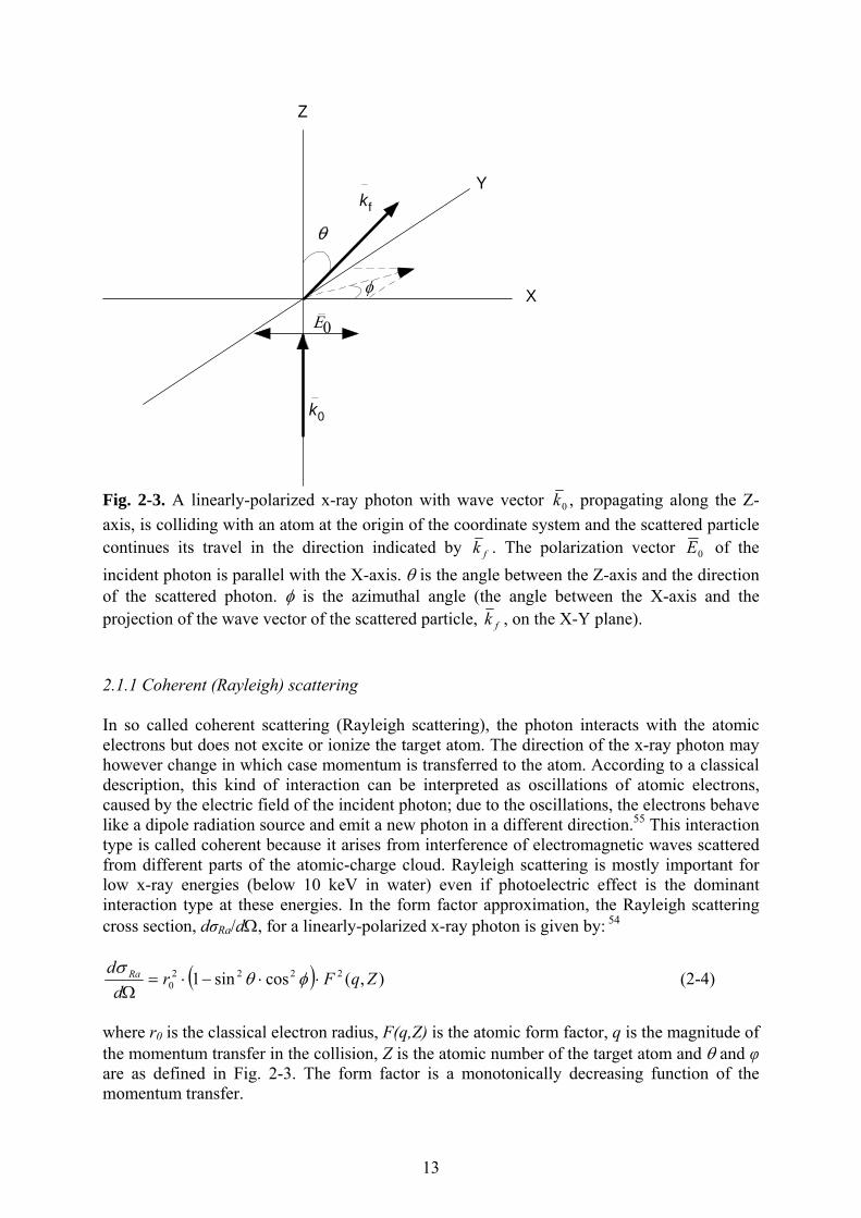
Fig. 2-2. X-ray interaction cross sections (EPDL).53 The differential scattering cross section for a polarized photon is a function of two angular variables (θ,φ).54 For unpolarized photons the direction of the scattered photon (or of the created photoelectron) is a function of the polar scattering angle, θ, only. The coordinate system that will be used in this section to describe scattering events is displayed in Fig. 2-3, where it is shown how a photon with propagation vector 0k and polarization vector 0E , traveling along the Z-axis, interacts with an atom at the origin and deflects into the direction of the scattered wave vector fk .
13
Y
X
Z
k0
kf
φ
Ε0
Fig. 2-3. A linearly-polarized x-ray photon with wave vector 0k , propagating along the Z-axis, is colliding with an atom at the origin of the coordinate system and the scattered particle continues its travel in the direction indicated by fk . The polarization vector 0E of the incident photon is parallel with the X-axis. θ is the angle between the Z-axis and the direction of the scattered photon. φ is the azimuthal angle (the angle between the X-axis and the projection of the wave vector of the scattered particle, fk , on the X-Y plane). 2.1.1 Coherent (Rayleigh) scattering In so called coherent scattering (Rayleigh scattering), the photon interacts with the atomic electrons but does not excite or ionize the target atom. The direction of the x-ray photon may however change in which case momentum is transferred to the atom. According to a classical description, this kind of interaction can be interpreted as oscillations of atomic electrons, caused by the electric field of the incident photon; due to the oscillations, the electrons behave like a dipole radiation source and emit a new photon in a different direction.55 This interaction type is called coherent because it arises from interference of electromagnetic waves scattered from different parts of the atomic-charge cloud. Rayleigh scattering is mostly important for low x-ray energies (below 10 keV in water) even if photoelectric effect is the dominant interaction type at these energies. In the form factor approximation, the Rayleigh scattering cross section, dσRa/dΩ, for a linearly-polarized x-ray photon is given by: 54
( ) ),(cossin1 22220 ZqFr
dd Ra ⋅⋅−⋅=Ω
φθσ
(2-4)
where r0 is the classical electron radius, F(q,Z) is the atomic form factor, q is the magnitude of the momentum transfer in the collision, Z is the atomic number of the target atom and θ and φ are as defined in Fig. 2-3. The form factor is a monotonically decreasing function of the momentum transfer.
14
In the limit of low x-ray energies and small momentum transfers, the Rayleigh total scattering cross section, σRa, is approximately given by: 45
2203
8 ZrRa ⋅⋅⋅≈ πσ (2-5)
2.1.2 Incoherent (Compton) scattering In a Compton scattering event, an x ray collides with an atomic electron and some of the x-ray energy is transferred to the electron which gets scattered away from the atom. In the theoretical description of Compton scattering, the electron is often considered as free and at rest. The entire energy lost by the photon in a collision is then transferred to kinetic energy of the electron. This is considered a sufficiently accurate description for medical physics applications since for x-ray energies where electron-binding energies and momentum distributions become important, the photoelectric effect is the dominating interaction type.56 For a free electron, the relation between the incoming and the scattered photon energy, υ⋅h and 'υ⋅h respectively, is given by the following expression:
)cos1(1'
20
θυυυ
−⋅⎟⎟⎠
⎞⎜⎜⎝
⎛⋅⋅
+
⋅=⋅
cmh
hh (2-6)
where h is Planck’s constant, υ is the photon frequency, 0m is the rest mass of the electron, c is the speed of light and θ is the polar scattering angle defined as in Fig. 2-3. The direction and kinetic energy of the Compton scattered electron is determined by energy and momentum conservation laws. Equation (2-6) is valid independently of the polarization direction. From the above formula it can be extracted that: 1) the minimum energy transfer in a Compton collision is obtained when the photon is scattered in the forward direction; then the scattering becomes purely elastic. The maximum energy is transferred to the electron when the photon is scattered in the backward (θ = 180 degrees) direction. 2) For lower x-ray energies, the fraction of the x-ray energy that is transferred to the electron decreases. In the limit of low x-ray energies, Compton scattering reduces to coherent scattering. Under the condition of a free electron at rest, the differential scattering cross-section for a linearly-polarized x-ray photon interacting with a free electron at rest is given by the Klein-Nishina formula: 57
⎟⎠⎞
⎜⎝⎛ ⋅⋅−
⋅⋅
+⋅⋅
⋅⎟⎠⎞
⎜⎝⎛
⋅⋅
⋅⋅=Ω
φθυυ
υυ
υυσ 22
22
0 cossin2'
''21
hh
hh
hhr
dd KN (2-7)
2.1.3 Photoelectric effect In the photoelectric effect, the entire photon energy is transferred to a bound electron which is ejected from the atom with a kinetic energy equal to the incident photon energy subtracted for the electron binding energy. The probability of photoelectric effect increases rapidly when the x-ray energy decreases, especially for high-Z materials, and it is the dominating interaction
15
type for low photon energies.56 When the x-ray energy is above the K-shell binding energy, the probability that a photoelectric effect occurs is largest in the K shell. After such inner-shell ionizations, the atoms are left in an excited state. For lower x-ray energies, the photoelectric effect is also to an increasing degree responsible for the larger energy transfers to secondary electrons since the energy transfer in the Compton collisions approaches zero. The angular distribution of the emitted photoelectrons is wider for lower x-ray energies and narrows in around zero degrees for increasing energies.56 However, the difference in the size of the photoemission angle, for incident x-rays from the lower to the higher end of the spectrum used for MRT, is only small. No single analytical expression of the photoelectric interaction cross section is valid for all x-ray energies and materials; however more precise tabulations of shell cross sections exist.53,58,59 The differential scattering cross section for the photoelectric effect (dσPh/dΩ), in the case of a hydrogen atom and for a polarized x-ray photon of energy much above the electron binding energy, is approximately given by the following expression: 51
4
22
50
5
0cos1
cossin)(2
32
⎟⎟⎠
⎞⎜⎜⎝
⎛⋅−
⋅⋅
⋅⋅⋅⋅⋅⎟⎟⎠
⎞⎜⎜⎝
⎛⋅⋅=
Ωe
f
ee
f
Ph
cvak
Zmh
dd
θ
φθυπ
ασ
(2-8)
where α is the fine structure constant, a0 is the Bohr radius, kf is the magnitude of the wave-vector of the photoelectron, vf is the velocity of the emitted photoelectron and the angular variables θ and φ are defined as in Fig. 2-3, now only with the subscript e to emphasize that it is an electron which is ejected in a certain angle and not the incident photon. Two aspects of interest in this work, which holds in the general case, can be extracted from formula (2-8): 1) photoelectron emission in zero (and 180) degrees in the polar angle is forbidden since this direction is perpendicular to the electric-field vector of the x ray. 2) for a linearly-polarized photon, photoelectron emission in φe = ± 90 degrees is also forbidden. 2.1.4 Atomic relaxation When an atom has been ionized and left in an excited state it can de-excite and return to its ground state by two processes, either by so called non-radiative transitions (also known as Auger transitions) or by x-ray emission. In the Auger process, an electron falls in to fill the vacancy of the electron which has been emitted in the ionization process. An electron from an outer electron shell is then emitted to release the atomic excess energy. This is repeated until the vacancy has migrated toward the outermost shell. Alternatively a radiative transition can occur in which case the excess energy is emitted as an x-ray photon followed by non-radiative transitions. In water or tissue (low-atomic-number materials), the atoms de-excite by Auger electron emission. For high-atomic-number materials, such as gold, the probability of x-ray emission increases. The probability that an x-ray is emitted after an ionization is called the fluorescence yield. The radiation energy transferred to a volume within a medium where an atomic inner-shell ionization has occurred depends partly on the fluorescence yield of the atoms building up the material. If the atoms de-excite mainly with Auger electron emission the excess energy is deposited near the excited atom. A fluorescent x ray on the other hand may travel a considerable distance from the atom of origin before it interacts and deposits its energy.
16
2.1.5 Attenuation of x-rays with depth in a medium The attenuation coefficient μ (or macroscopic cross-section) is defined as the sum of the relevant cross sections multiplied by the number of atoms per unit volume. If μ is divided by the density of the medium the mass attenuation coefficient (μ/ρ) is obtained. Tabulated values of (μ/ρ) are found in publicly available databases.59 To calculate the fraction of primary photons which have reached a certain depth x in a material, without being scattered, the so called Lambert-Beers law can be used. It gives the intensity B of a monoenergetic beam at a depth x:
⎟⎟⎠
⎞⎜⎜⎝
⎛⋅⋅−
⋅=x
eBxBρ
ρμ
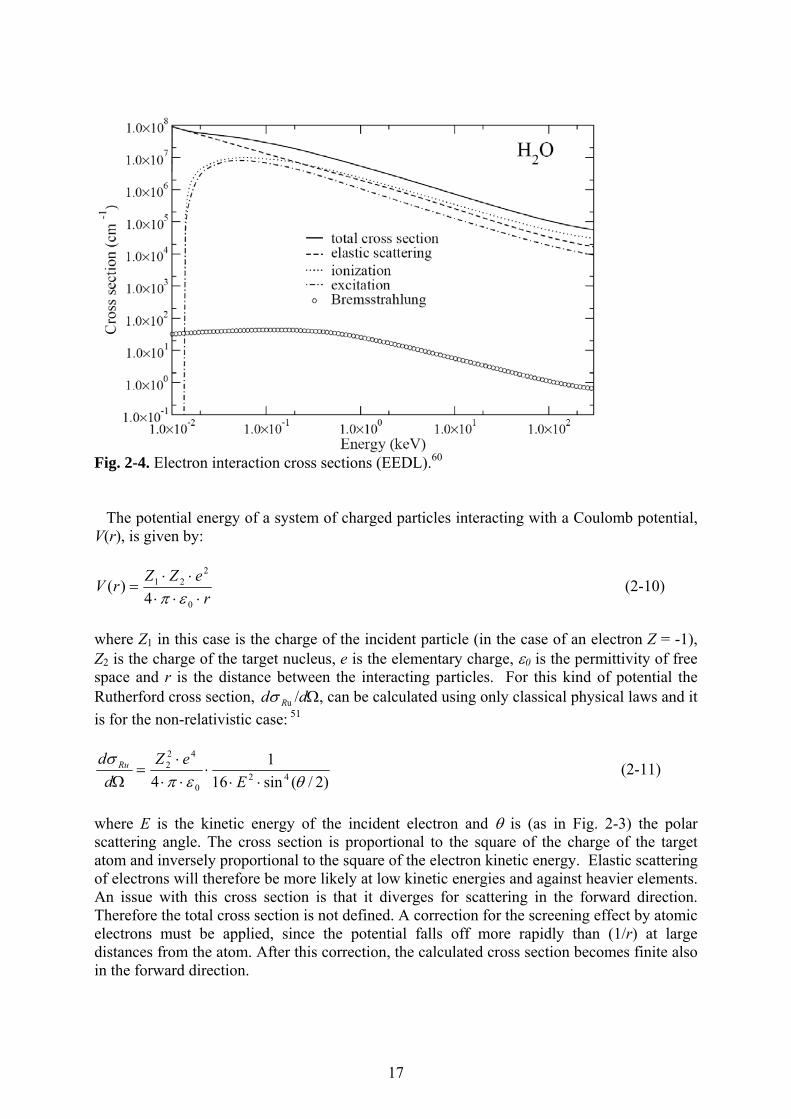
0)( (2-9) where B0 is the surface (initial) intensity. The same calculation can be done for a beam containing a spectrum of x-ray energies but would be slightly more complicated due to the discretization needed. It should be emphasized that the intensity of secondary photons is unaccounted for in equation (2-9). Measurements of the attenuation coefficient are always done with a narrow collimated beam in order to avoid contributions from scattered radiation. 2.2 Secondary electron interactions with matter Photons lose their energy in a few collisions, ending with the photon being absorbed, while an electron loses its energy in many small collisions. Electrons therefore ionize numerous atoms in their slowing-down process. In x-ray irradiations of water (for x-rays in the spectral range shown in Fig. 2-1), most of the ionizations and excitations are produced by the secondary electrons.56 The electron interactions can be divided in elastic scattering, inelastic scattering and Bremsstrahlung emission. In Fig. 2-4, electron interaction cross sections in water from the Evaluated Electron Data Library60 (EEDL) are shown. For secondary electrons traveling in water with energies relevant for MRT (< 300 keV), there is a negligible probability of Bremsstrahlung emission. 2.2.1 Elastic scattering: In elastic scattering (by definition) the final quantum state of the target atom (after the collision) is the same as the initial quantum state (before the collision).45 In an elastic collision, the electron does not lose energy in exciting the scattering atom, but its direction is changed. There is actually a very small energy transfer given to the scattering atom in the form of kinetic energy, but it is so small that it is usually neglected. (The energy transfer is small because the mass of the scattering atom is much larger than the mass of the electron.) An electron which is moving inside a medium is continuously interacting with the Coulomb field of nearly every atom it passes along its path which changes its travel direction. Elastic scattering against the atomic nucleus gives rise to larger angular deflections than scattering against the atomic electrons.56 Since the cross section for elastic electron scattering is large (compared to what it is for inelastic electron interactions (see Fig. 2-4)) an electron normally experiences a large number of elastic collisions before reaching the end of its path.
17
Fig. 2-4. Electron interaction cross sections (EEDL).60 The potential energy of a system of charged particles interacting with a Coulomb potential, V(r), is given by:
reZZrV⋅⋅⋅⋅⋅
=0
221
4)(
επ (2-10)
where Z1 in this case is the charge of the incident particle (in the case of an electron Z = -1), Z2 is the charge of the target nucleus, e is the elementary charge, ε0 is the permittivity of free space and r is the distance between the interacting particles. For this kind of potential the Rutherford cross section, uRdσ /dΩ, can be calculated using only classical physical laws and it is for the non-relativistic case: 51
)2/(sin161
4 420
422
θεπσ
⋅⋅⋅
⋅⋅⋅
=Ω E
eZd
d Ru (2-11)
where E is the kinetic energy of the incident electron and θ is (as in Fig. 2-3) the polar scattering angle. The cross section is proportional to the square of the charge of the target atom and inversely proportional to the square of the electron kinetic energy. Elastic scattering of electrons will therefore be more likely at low kinetic energies and against heavier elements. An issue with this cross section is that it diverges for scattering in the forward direction. Therefore the total cross section is not defined. A correction for the screening effect by atomic electrons must be applied, since the potential falls off more rapidly than (1/r) at large distances from the atom. After this correction, the calculated cross section becomes finite also in the forward direction.
18
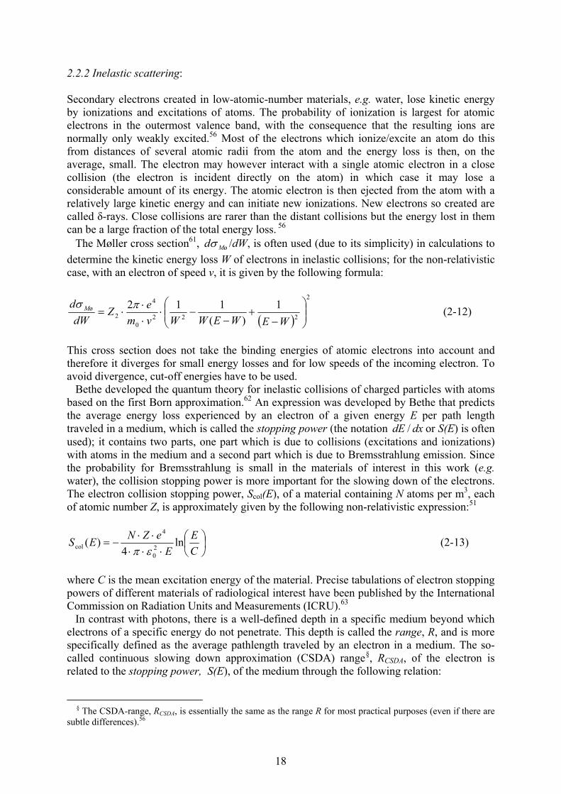
2.2.2 Inelastic scattering: Secondary electrons created in low-atomic-number materials, e.g. water, lose kinetic energy by ionizations and excitations of atoms. The probability of ionization is largest for atomic electrons in the outermost valence band, with the consequence that the resulting ions are normally only weakly excited.56 Most of the electrons which ionize/excite an atom do this from distances of several atomic radii from the atom and the energy loss is then, on the average, small. The electron may however interact with a single atomic electron in a close collision (the electron is incident directly on the atom) in which case it may lose a considerable amount of its energy. The atomic electron is then ejected from the atom with a relatively large kinetic energy and can initiate new ionizations. New electrons so created are called δ-rays. Close collisions are rarer than the distant collisions but the energy lost in them can be a large fraction of the total energy loss. 56 The Møller cross section61, øMdσ /dW, is often used (due to its simplicity) in calculations to determine the kinetic energy loss W of electrons in inelastic collisions; for the non-relativistic case, with an electron of speed v, it is given by the following formula:
( )
2
2220
4
2ø 1
)(112
⎟⎟⎠
⎞⎜⎜⎝
⎛
−+
−−⋅
⋅⋅
⋅=WEWEWWvm
eZdW
d M πσ (2-12)
This cross section does not take the binding energies of atomic electrons into account and therefore it diverges for small energy losses and for low speeds of the incoming electron. To avoid divergence, cut-off energies have to be used. Bethe developed the quantum theory for inelastic collisions of charged particles with atoms based on the first Born approximation.62 An expression was developed by Bethe that predicts the average energy loss experienced by an electron of a given energy E per path length traveled in a medium, which is called the stopping power (the notation dxdE / or S(E) is often used); it contains two parts, one part which is due to collisions (excitations and ionizations) with atoms in the medium and a second part which is due to Bremsstrahlung emission. Since the probability for Bremsstrahlung is small in the materials of interest in this work (e.g. water), the collision stopping power is more important for the slowing down of the electrons. The electron collision stopping power, Scol(E), of a material containing N atoms per m3, each of atomic number Z, is approximately given by the following non-relativistic expression:51
⎟⎠⎞
⎜⎝⎛
⋅⋅⋅⋅⋅
−=CE
EeZNES ln
4)( 2
0
4
col επ (2-13)
where C is the mean excitation energy of the material. Precise tabulations of electron stopping powers of different materials of radiological interest have been published by the International Commission on Radiation Units and Measurements (ICRU).63 In contrast with photons, there is a well-defined depth in a specific medium beyond which electrons of a specific energy do not penetrate. This depth is called the range, R, and is more specifically defined as the average pathlength traveled by an electron in a medium. The so-called continuous slowing down approximation (CSDA) range§, RCSDA, of the electron is related to the stopping power, S(E), of the medium through the following relation:
§ The CSDA-range, RCSDA, is essentially the same as the range R for most practical purposes (even if there are subtle differences).56
19
dEESR ECSDA
⋅
=
∫max
0
)(
1 (2-14)
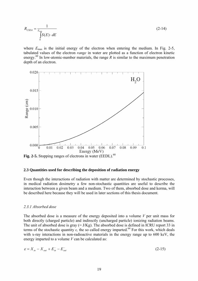
where Emax is the initial energy of the electron when entering the medium. In Fig. 2-5, tabulated values of the electron range in water are plotted as a function of electron kinetic energy.60 In low-atomic-number materials, the range R is similar to the maximum penetration depth of an electron.
Fig. 2-5. Stopping ranges of electrons in water (EEDL).60 2.3 Quantities used for describing the deposition of radiation energy Even though the interactions of radiation with matter are determined by stochastic processes, in medical radiation dosimetry a few non-stochastic quantities are useful to describe the interaction between a given beam and a medium. Two of them, absorbed dose and kerma, will be described here because they will be used in later sections of this thesis document. 2.3.1 Absorbed dose The absorbed dose is a measure of the energy deposited into a volume V per unit mass for both directly (charged particle) and indirectly (uncharged particle) ionizing radiation beams. The unit of absorbed dose is gray (= J/Kg). The absorbed dose is defined in ICRU report 33 in terms of the stochastic quantity ε, the so called energy imparted.64 For this work, which deals with x-ray interactions in non-radioactive materials in the energy range up to 600 keV, the energy imparted to a volume V can be calculated as:
−− −+−= outinoutin EEXXε (2-15)
20
where Xin and Xout is the total energy of all x-rays entering/leaving the volume V respectively and −
inE and −outE is the total kinetic energy of all electrons entering/leaving the volume V
respectively. The absorbed dose D is then calculated as:
MEXD )(ε
= (2-16)
where EX denotes expectation value and M is the mass of the detecting medium in the volume V. 2.3.2 Kerma (Kinetic energy released in matter) Kerma describes the energy transferred by indirectly ionizing radiation (in this case x-rays) to charged particles, in a certain volume V, per unit mass of a specific material.64 The unit of kerma is also gray (= J/Kg). For this work which deals with x-ray interactions in non-radioactive materials (for x-ray energies up to 600 keV), the so called energy transferred, εtr (a stochastic quantity), to a volume V can be obtained as:
*outintr XX −=ε (2-17)
where Xin is the total energy of all the x-rays entering into the volume V and *
outX is the total energy of x-rays leaving the volume V, except for x-rays which are due to Bremsstrahlung events. The kerma K is then calculated as:
MEX
K tr )(ε= (2-18)
where EX denotes expectation value and M is the mass of the detecting medium in the volume V.
21
3. MONTE CARLO SIMULATIONS OF DOSE DEPOSITION 3.1 The PENELOPE MC code PENELOPE is a general-purpose MC simulation package for coupled electron-photon transport in arbitrary materials.45 The developers of this code have put special emphasis on the implementation of precise low-energy electron/photon cross sections and the code has been widely used in medical-physics applications.46-50 In this work the 2003 version of the code was used. In PENELOPE, cross sections for unpolarized photons are implemented. Unfortunately, no existing MC code has differential cross sections for polarized x-ray photons incorporated for all relevant interaction types. For photons (unpolarized), the interaction cross sections for photoelectric effect, coherent-, and Compton-scattering, all relevant for the MRT application, are implemented in the code. The photon interactions are simulated collision by collision until the photon energy falls below the absorption threshold set in the initialization of the simulation run. For the x-ray spectrum generated by the ESRF wiggler (see Fig. 2-1), Compton scattering is the most likely primary-photon interaction type in low-atomic-number materials of interest. When simulating Compton interactions, as corrections to the Klein-Nishina formula, PENELOPE considers the influence of electron-binding and of the momentum distributions of atomic electrons. These two effects are of minor importance at x-ray energies far above any absorption edge; nevertheless, most x rays experience several Compton collisions before being absorbed and therefore the secondary photon spectrum is shifted towards lower energies which eventually might make these corrections important. The electron interactions to be considered in MRT-MC dosimetry are elastic scattering and ionization/excitation. The simulation model used for the elastic scattering of low-energy electrons, generated in Compton interactions and in photoelectric absorption, is of particular importance since it determines how far away from the microbeams (into the valley dose region) electrons of a certain energy are transported. For elastic electron scattering, PENELOPE uses a modified Wentzel distribution with parameters obtained from relativistic partial-wave analysis.45 For electron-impact ionization a generalized oscillator-strength model is used, set to reproduce the mean ionization potential of the particular material. This model has been shown to give stopping-power values in good agreement with data tabulated in ICRU 37.63
A mixed simulation scheme for electrons is implemented in the code, according to established terminology,65 where electron interactions with large energy losses and large angular deflections (inelastic and elastic collisions, respectively) are simulated in detail, collision by collision, while small energy losses and angular deflections are treated in a grouped manner. The user defined parameters C1 ( )cos(11 θ−=C , determining the average deflection angle produced by multiple elastic scattering along a path length equal to the mean free path between consecutive hard elastic events), C2 (the maximum average fractional energy loss allowed between consecutive hard elastic events), and WCC (cutoff energy loss for hard inelastic collisions) in the mixed simulation algorithm can be set to run the simulation along a scale from purely detailed simulation of all collisions to a grouping of many electron collisions along a single MC step. For the simulations done in this work the detailed mode was preferentially used. This was possible since the generated secondary electrons are of relatively low energy and therefore they suffer comparatively few collisions before being absorbed.
22
3.2 Simulation geometry and details In this thesis work two different microbeam shapes were considered for MC simulations: a cylindrical (circular-shaped) and a planar (narrow-rectangular) beam. A cylindrical water phantom with constant dimensions of 16 cm in diameter and 16 cm in height was used for scoring the dose in the simulations. The choice of beam shapes and phantom was based on having the same phantom material and dimensions as used in earlier studies of MRT.13,30,31 In most of the calculations, the x-ray energies were sampled from the measured spectrum at the ID17 beamline. This spectrum, shown in Fig. 2-1, contains photons in the interval from 30 keV up to 600 keV with a mean energy of 107 keV. However, the fraction of photons with energies above 300 keV is small. For comparison, simulations using 50-, 100-, 150- and 200-keV monoenergetic beams were also performed for a few selected cases. Parts of this work has been published in Siegbahn et al.66
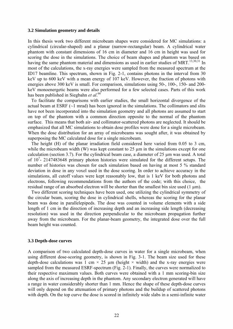
To facilitate the comparisons with earlier studies, the small horizontal divergence of the actual beam at ESRF (~1 mrad) has been ignored in the simulations. The collimators and slits have not been incorporated into the simulation geometry and all photons are assumed to start on top of the phantom with a common direction opposite to the normal of the phantom surface. This means that both air- and collimator-scattered photons are neglected. It should be emphasized that all MC simulations to obtain dose profiles were done for a single microbeam. When the dose distribution for an array of microbeams was sought after, it was obtained by superposing the MC calculated dose for a single microbeam. The height (H) of the planar irradiation field considered here varied from 0.05 to 3 cm, while the microbeam width (W) was kept constant to 25 µm in the simulations except for one calculation (section 3.7). For the cylindrical beam case, a diameter of 25 µm was used. A total of 107- 2147483648 primary photon histories were simulated for the different setups. The number of histories was chosen for each simulation based on having at most 5 % standard deviation in dose in any voxel used in the dose scoring. In order to achieve accuracy in the simulations, all cutoff values were kept reasonably low, that is 1 keV for both photons and electrons, following recommendations from the authors of the code; with this choice, the residual range of an absorbed electron will be shorter than the smallest bin size used (1 µm). Two different scoring techniques have been used, one utilizing the cylindrical symmetry of the circular beam, scoring the dose in cylindrical shells, whereas the scoring for the planar beam was done in parallelepipeds. The dose was counted in volume elements with a side length of 1 cm in the direction of increasing depth and an increasing side length (decreasing resolution) was used in the direction perpendicular to the microbeam propagation further away from the microbeam. For the planar-beam geometry, the integrated dose over the full beam height was counted. 3.3 Depth-dose curves A comparison of two calculated depth-dose curves in water for a single microbeam, when using different dose-scoring geometry, is shown in Fig. 3-1. The beam size used for these depth-dose calculations was 1 cm × 25 µm (height × width) and the x-ray energies were sampled from the measured ESRF-spectrum (Fig. 2-1). Finally, the curves were normalized to their respective maximum values. Both curves were obtained with a 1 mm scoring-bin size along the axis of increasing depth in the phantom. Any secondary electron generated will have a range in water considerably shorter than 1 mm. Hence the shape of these depth-dose curves will only depend on the attenuation of primary photons and the buildup of scattered photons with depth. On the top curve the dose is scored in infinitely wide slabs in a semi-infinite water
23
phantom. The important characteristic of this dose-scoring geometry (which is normally called a broad-beam geometry56) is that a large part of the scattered radiation is detected. For this slab-scoring geometry the dose maximum is found at a depth of about 1.4 cm from the surface. For the lower curve (central-axis scoring), the dose is scored in voxels that are just as wide as the beam along the beam central axis. This depth-dose curve shows an immediate decrease with depth and that the microbeam dose half-value layer, for the ESRF x-ray spectrum and the beam size mentioned above, is approximately 4.2 cm of water. The dose deposition outside the primary microbeam field must therefore be increasing with depth over the first centimeter. As it will be discussed later on in this chapter, this observation is essential for understanding the variation of PVDR’s with depth.
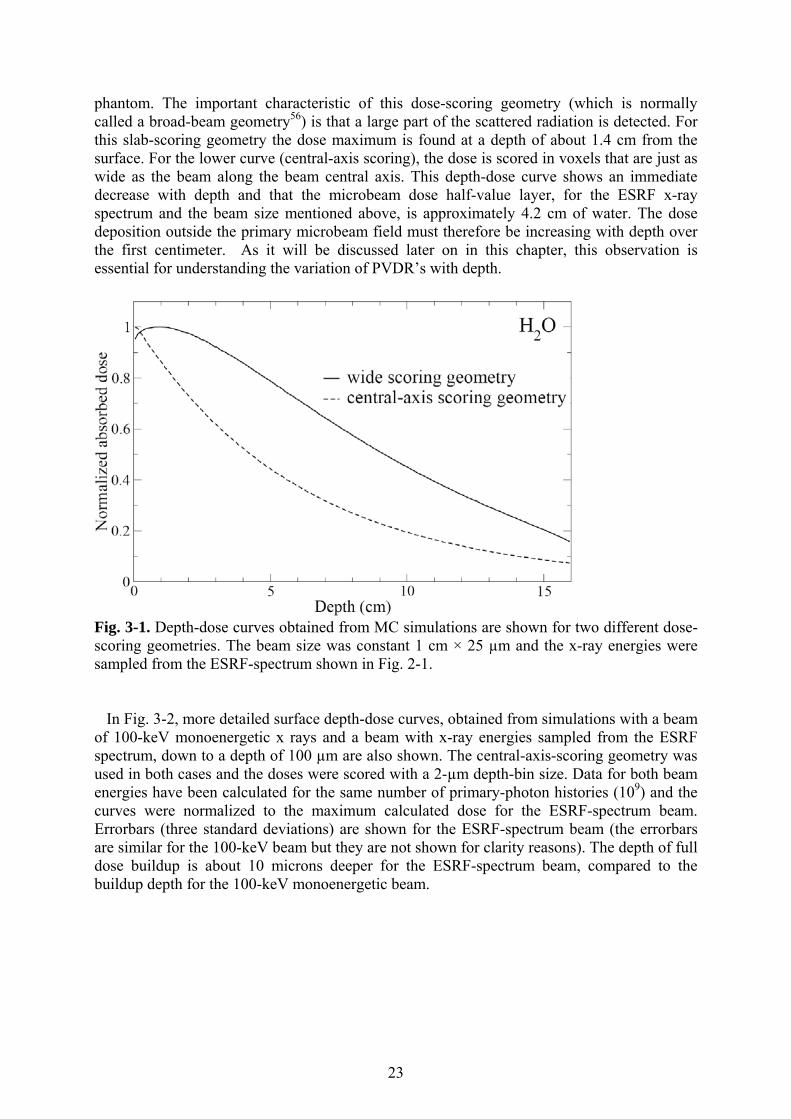
Fig. 3-1. Depth-dose curves obtained from MC simulations are shown for two different dose-scoring geometries. The beam size was constant 1 cm × 25 µm and the x-ray energies were sampled from the ESRF-spectrum shown in Fig. 2-1. In Fig. 3-2, more detailed surface depth-dose curves, obtained from simulations with a beam of 100-keV monoenergetic x rays and a beam with x-ray energies sampled from the ESRF spectrum, down to a depth of 100 µm are also shown. The central-axis-scoring geometry was used in both cases and the doses were scored with a 2-µm depth-bin size. Data for both beam energies have been calculated for the same number of primary-photon histories (109) and the curves were normalized to the maximum calculated dose for the ESRF-spectrum beam. Errorbars (three standard deviations) are shown for the ESRF-spectrum beam (the errorbars are similar for the 100-keV beam but they are not shown for clarity reasons). The depth of full dose buildup is about 10 microns deeper for the ESRF-spectrum beam, compared to the buildup depth for the 100-keV monoenergetic beam.
24
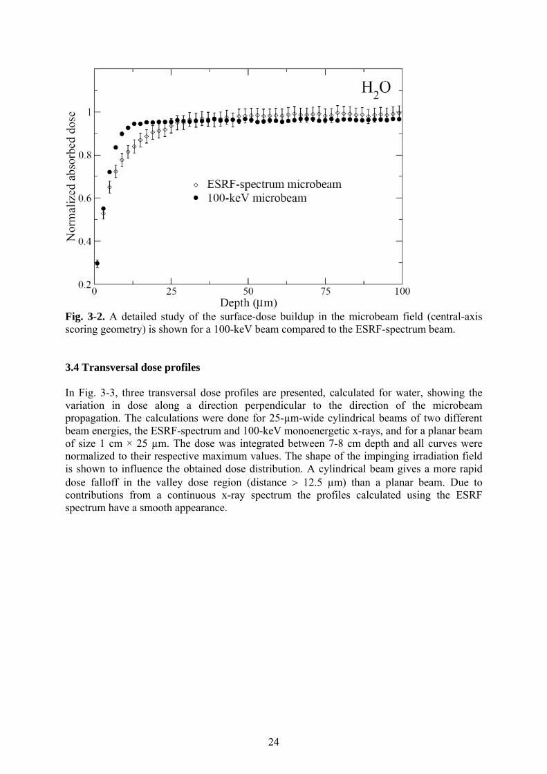
Fig. 3-2. A detailed study of the surface-dose buildup in the microbeam field (central-axis scoring geometry) is shown for a 100-keV beam compared to the ESRF-spectrum beam. 3.4 Transversal dose profiles In Fig. 3-3, three transversal dose profiles are presented, calculated for water, showing the variation in dose along a direction perpendicular to the direction of the microbeam propagation. The calculations were done for 25-µm-wide cylindrical beams of two different beam energies, the ESRF-spectrum and 100-keV monoenergetic x-rays, and for a planar beam of size 1 cm × 25 µm. The dose was integrated between 7-8 cm depth and all curves were normalized to their respective maximum values. The shape of the impinging irradiation field is shown to influence the obtained dose distribution. A cylindrical beam gives a more rapid dose falloff in the valley dose region (distance > 12.5 µm) than a planar beam. Due to contributions from a continuous x-ray spectrum the profiles calculated using the ESRF spectrum have a smooth appearance.
25
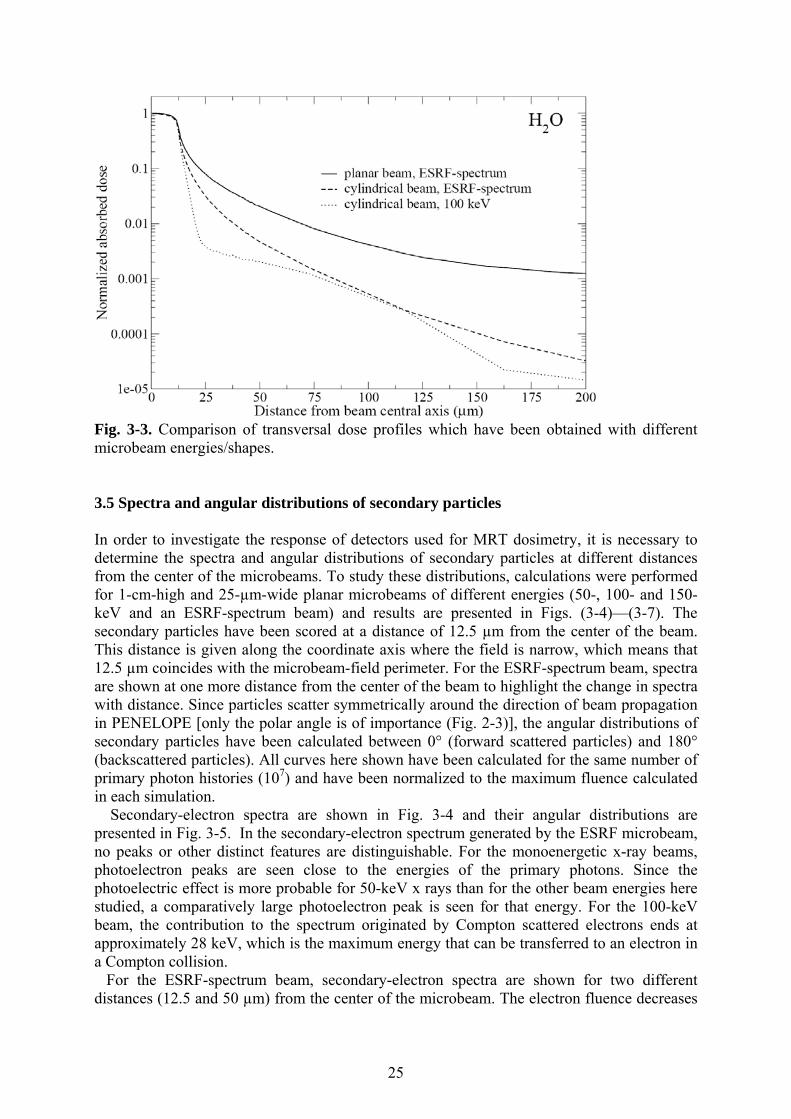
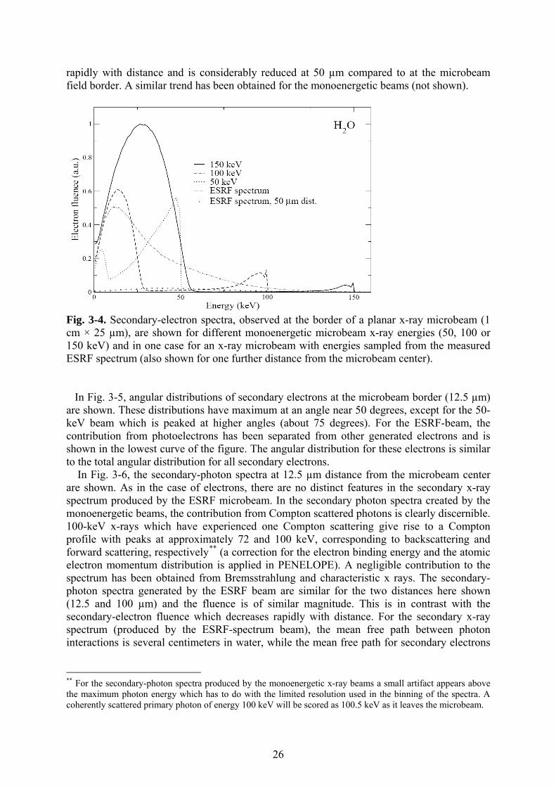
Fig. 3-3. Comparison of transversal dose profiles which have been obtained with different microbeam energies/shapes. 3.5 Spectra and angular distributions of secondary particles In order to investigate the response of detectors used for MRT dosimetry, it is necessary to determine the spectra and angular distributions of secondary particles at different distances from the center of the microbeams. To study these distributions, calculations were performed for 1-cm-high and 25-µm-wide planar microbeams of different energies (50-, 100- and 150-keV and an ESRF-spectrum beam) and results are presented in Figs. (3-4)—(3-7). The secondary particles have been scored at a distance of 12.5 µm from the center of the beam. This distance is given along the coordinate axis where the field is narrow, which means that 12.5 µm coincides with the microbeam-field perimeter. For the ESRF-spectrum beam, spectra are shown at one more distance from the center of the beam to highlight the change in spectra with distance. Since particles scatter symmetrically around the direction of beam propagation in PENELOPE [only the polar angle is of importance (Fig. 2-3)], the angular distributions of secondary particles have been calculated between 0° (forward scattered particles) and 180° (backscattered particles). All curves here shown have been calculated for the same number of primary photon histories (107) and have been normalized to the maximum fluence calculated in each simulation. Secondary-electron spectra are shown in Fig. 3-4 and their angular distributions are presented in Fig. 3-5. In the secondary-electron spectrum generated by the ESRF microbeam, no peaks or other distinct features are distinguishable. For the monoenergetic x-ray beams, photoelectron peaks are seen close to the energies of the primary photons. Since the photoelectric effect is more probable for 50-keV x rays than for the other beam energies here studied, a comparatively large photoelectron peak is seen for that energy. For the 100-keV beam, the contribution to the spectrum originated by Compton scattered electrons ends at approximately 28 keV, which is the maximum energy that can be transferred to an electron in a Compton collision. For the ESRF-spectrum beam, secondary-electron spectra are shown for two different distances (12.5 and 50 µm) from the center of the microbeam. The electron fluence decreases
26
rapidly with distance and is considerably reduced at 50 µm compared to at the microbeam field border. A similar trend has been obtained for the monoenergetic beams (not shown).
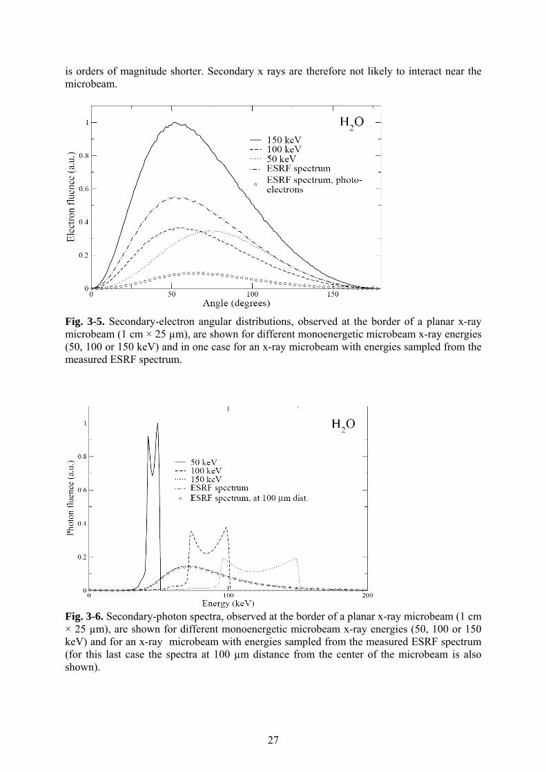
Fig. 3-4. Secondary-electron spectra, observed at the border of a planar x-ray microbeam (1 cm × 25 µm), are shown for different monoenergetic microbeam x-ray energies (50, 100 or 150 keV) and in one case for an x-ray microbeam with energies sampled from the measured ESRF spectrum (also shown for one further distance from the microbeam center). In Fig. 3-5, angular distributions of secondary electrons at the microbeam border (12.5 µm) are shown. These distributions have maximum at an angle near 50 degrees, except for the 50-keV beam which is peaked at higher angles (about 75 degrees). For the ESRF-beam, the contribution from photoelectrons has been separated from other generated electrons and is shown in the lowest curve of the figure. The angular distribution for these electrons is similar to the total angular distribution for all secondary electrons. In Fig. 3-6, the secondary-photon spectra at 12.5 µm distance from the microbeam center are shown. As in the case of electrons, there are no distinct features in the secondary x-ray spectrum produced by the ESRF microbeam. In the secondary photon spectra created by the monoenergetic beams, the contribution from Compton scattered photons is clearly discernible. 100-keV x-rays which have experienced one Compton scattering give rise to a Compton profile with peaks at approximately 72 and 100 keV, corresponding to backscattering and forward scattering, respectively** (a correction for the electron binding energy and the atomic electron momentum distribution is applied in PENELOPE). A negligible contribution to the spectrum has been obtained from Bremsstrahlung and characteristic x rays. The secondary-photon spectra generated by the ESRF beam are similar for the two distances here shown (12.5 and 100 µm) and the fluence is of similar magnitude. This is in contrast with the secondary-electron fluence which decreases rapidly with distance. For the secondary x-ray spectrum (produced by the ESRF-spectrum beam), the mean free path between photon interactions is several centimeters in water, while the mean free path for secondary electrons
** For the secondary-photon spectra produced by the monoenergetic x-ray beams a small artifact appears above the maximum photon energy which has to do with the limited resolution used in the binning of the spectra. A coherently scattered primary photon of energy 100 keV will be scored as 100.5 keV as it leaves the microbeam.
27
is orders of magnitude shorter. Secondary x rays are therefore not likely to interact near the microbeam.
Fig. 3-5. Secondary-electron angular distributions, observed at the border of a planar x-ray microbeam (1 cm × 25 µm), are shown for different monoenergetic microbeam x-ray energies (50, 100 or 150 keV) and in one case for an x-ray microbeam with energies sampled from the measured ESRF spectrum.
Fig. 3-6. Secondary-photon spectra, observed at the border of a planar x-ray microbeam (1 cm × 25 µm), are shown for different monoenergetic microbeam x-ray energies (50, 100 or 150 keV) and for an x-ray microbeam with energies sampled from the measured ESRF spectrum (for this last case the spectra at 100 µm distance from the center of the microbeam is also shown).
28
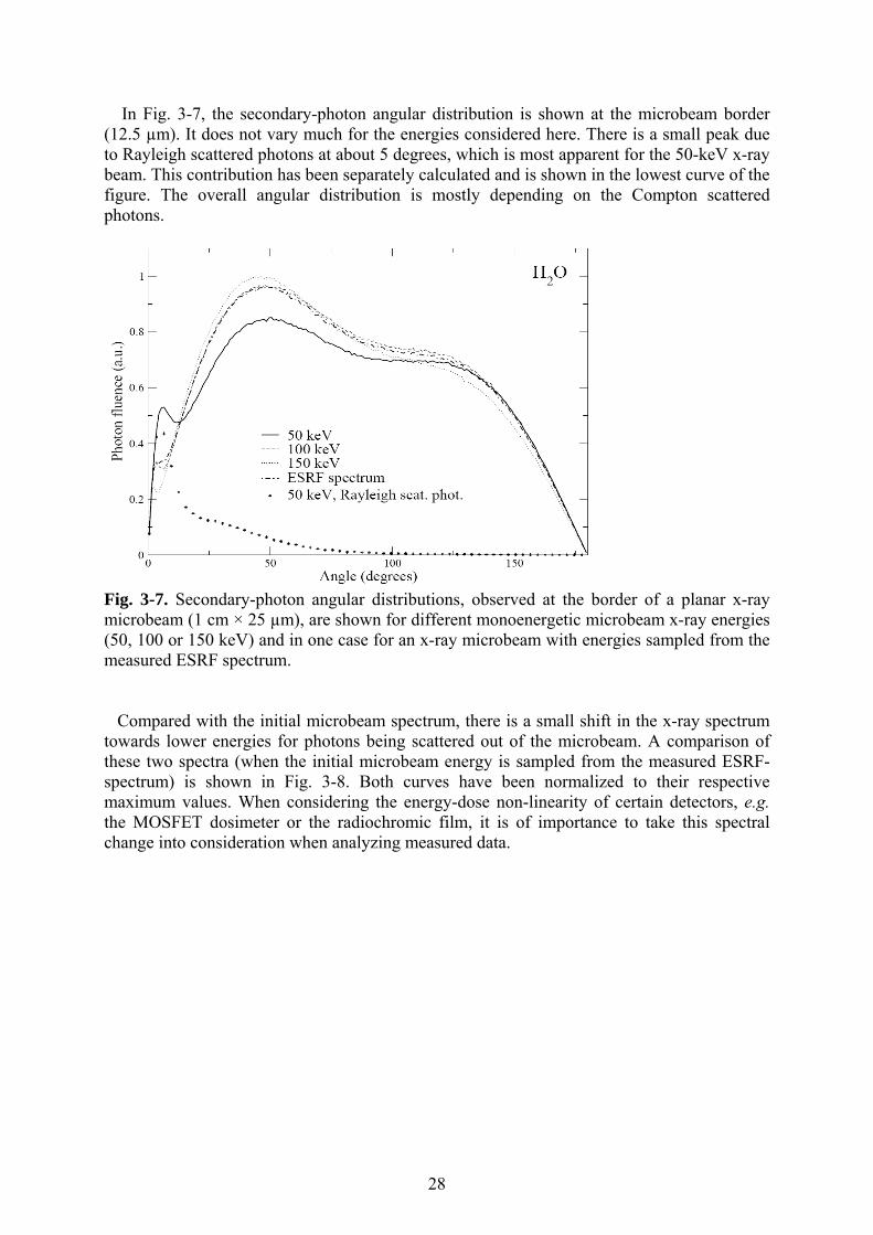
In Fig. 3-7, the secondary-photon angular distribution is shown at the microbeam border (12.5 µm). It does not vary much for the energies considered here. There is a small peak due to Rayleigh scattered photons at about 5 degrees, which is most apparent for the 50-keV x-ray beam. This contribution has been separately calculated and is shown in the lowest curve of the figure. The overall angular distribution is mostly depending on the Compton scattered photons.
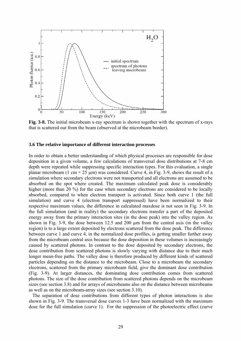
Fig. 3-7. Secondary-photon angular distributions, observed at the border of a planar x-ray microbeam (1 cm × 25 µm), are shown for different monoenergetic microbeam x-ray energies (50, 100 or 150 keV) and in one case for an x-ray microbeam with energies sampled from the measured ESRF spectrum. Compared with the initial microbeam spectrum, there is a small shift in the x-ray spectrum towards lower energies for photons being scattered out of the microbeam. A comparison of these two spectra (when the initial microbeam energy is sampled from the measured ESRF-spectrum) is shown in Fig. 3-8. Both curves have been normalized to their respective maximum values. When considering the energy-dose non-linearity of certain detectors, e.g. the MOSFET dosimeter or the radiochromic film, it is of importance to take this spectral change into consideration when analyzing measured data.
29
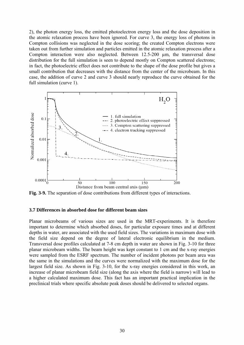
Fig. 3-8. The initial microbeam x-ray spectrum is shown together with the spectrum of x-rays that is scattered out from the beam (observed at the microbeam border). 3.6 The relative importance of different interaction processes In order to obtain a better understanding of which physical processes are responsible for dose deposition in a given volume, a few calculations of transversal dose distributions at 7-8 cm depth were repeated while suppressing specific interaction types. For this evaluation, a single planar microbeam (1 cm × 25 µm) was considered. Curve 4, in Fig. 3-9, shows the result of a simulation where secondary electrons were not transported and all electrons are assumed to be absorbed on the spot where created. The maximum calculated peak dose is considerably higher (more than 20 %) for the case when secondary electrons are considered to be locally absorbed, compared to when electron transport is activated. Since both curve 1 (the full simulation) and curve 4 (electron transport suppressed) have been normalized to their respective maximum values, the difference in calculated maxdose is not seen in Fig. 3-9. In the full simulation (and in reality) the secondary electrons transfer a part of the deposited energy away from the primary interaction sites (in the dose peak) into the valley region. As shown in Fig. 3-9, the dose between 12.5 and 200 µm from the central axis (in the valley region) is to a large extent deposited by electrons scattered from the dose peak. The difference between curve 1 and curve 4, in the normalized dose profiles, is getting smaller further away from the microbeam central axis because the dose deposition in these volumes is increasingly caused by scattered photons. In contrast to the dose deposited by secondary electrons, the dose contribution from scattered photons is slowly varying with distance due to their much longer mean-free paths. The valley dose is therefore produced by different kinds of scattered particles depending on the distance to the microbeam. Close to a microbeam the secondary electrons, scattered from the primary microbeam field, give the dominant dose contribution (Fig. 3-9). At larger distances, the dominating dose contribution comes from scattered photons. The size of the dose contribution from scattered photons depends on the microbeam sizes (see section 3.8) and for arrays of microbeams also on the distance between microbeams as well as on the microbeam-array sizes (see section 3.10). The separation of dose contributions from different types of photon interactions is also shown in Fig. 3-9. The transversal dose curves 1-3 have been normalized with the maximum dose for the full simulation (curve 1). For the suppression of the photoelectric effect (curve
30
2), the photon energy loss, the emitted photoelectron energy loss and the dose deposition in the atomic relaxation process have been ignored. For curve 3, the energy loss of photons in Compton collisions was neglected in the dose scoring; the created Compton electrons were taken out from further simulation and particles emitted in the atomic relaxation process after a Compton interaction were also neglected. Between 12.5-200 µm, the transversal dose distribution for the full simulation is seen to depend mostly on Compton scattered electrons; in fact, the photoelectric effect does not contribute to the shape of the dose profile but gives a small contribution that decreases with the distance from the center of the microbeam. In this case, the addition of curve 2 and curve 3 should nearly reproduce the curve obtained for the full simulation (curve 1).
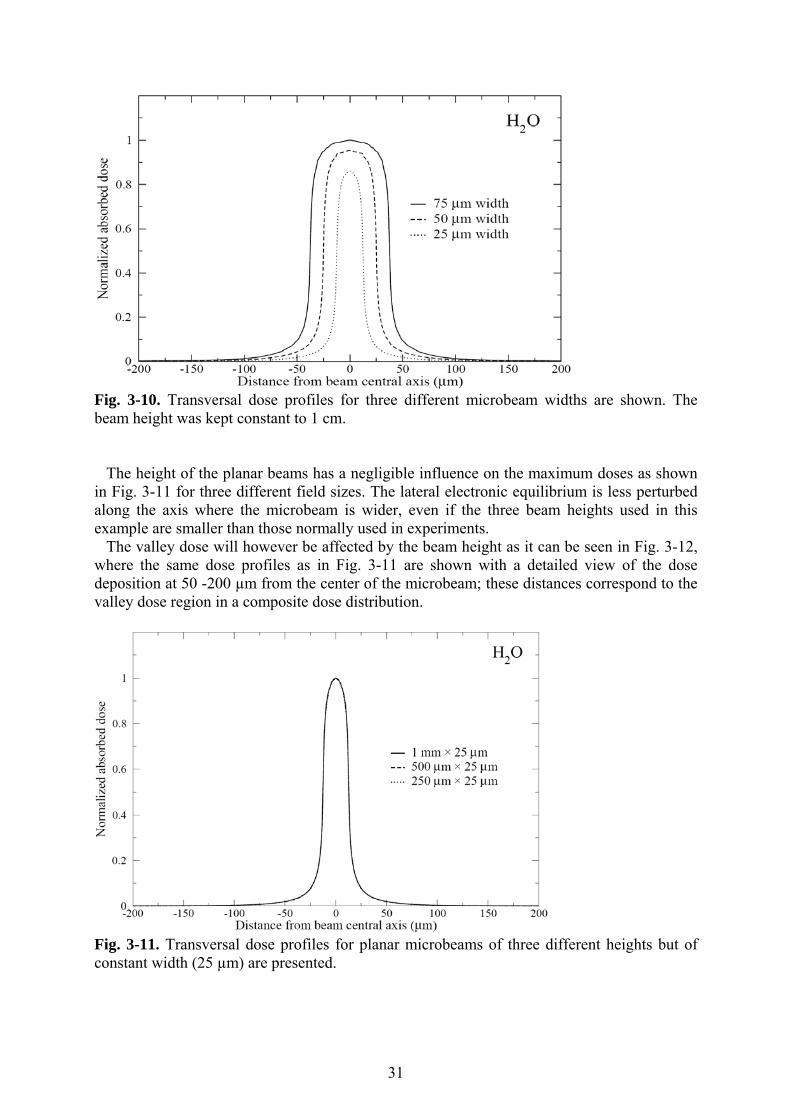
Fig. 3-9. The separation of dose contributions from different types of interactions. 3.7 Differences in absorbed dose for different beam sizes Planar microbeams of various sizes are used in the MRT-experiments. It is therefore important to determine which absorbed doses, for particular exposure times and at different depths in water, are associated with the used field sizes. The variations in maximum dose with the field size depend on the degree of lateral electronic equilibrium in the medium. Transversal dose profiles calculated at 7-8 cm depth in water are shown in Fig. 3-10 for three planar microbeam widths. The beam height was kept constant to 1 cm and the x-ray energies were sampled from the ESRF spectrum. The number of incident photons per beam area was the same in the simulations and the curves were normalized with the maximum dose for the largest field size. As shown in Fig. 3-10, for the x-ray energies considered in this work, an increase of planar microbeam field size (along the axis where the field is narrow) will lead to a higher calculated maximum dose. This fact has an important practical implication in the preclinical trials where specific absolute peak doses should be delivered to selected organs.
31
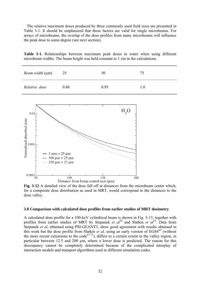
Fig. 3-10. Transversal dose profiles for three different microbeam widths are shown. The beam height was kept constant to 1 cm. The height of the planar beams has a negligible influence on the maximum doses as shown in Fig. 3-11 for three different field sizes. The lateral electronic equilibrium is less perturbed along the axis where the microbeam is wider, even if the three beam heights used in this example are smaller than those normally used in experiments. The valley dose will however be affected by the beam height as it can be seen in Fig. 3-12, where the same dose profiles as in Fig. 3-11 are shown with a detailed view of the dose deposition at 50 -200 µm from the center of the microbeam; these distances correspond to the valley dose region in a composite dose distribution.
Fig. 3-11. Transversal dose profiles for planar microbeams of three different heights but of constant width (25 µm) are presented.
32
The relative maximum doses produced by three commonly used field sizes are presented in Table 3-1. It should be emphasized that these factors are valid for single microbeams. For arrays of microbeams, the overlap of the dose profiles from many microbeams will influence the peak dose to some degree (see next section). Table 3-1. Relationships between maximum peak doses in water when using different microbeam widths. The beam height was held constant to 1 cm in the calculations. Beam width (µm)
25
50
75
Relative dose
0.86
0.95
1.0
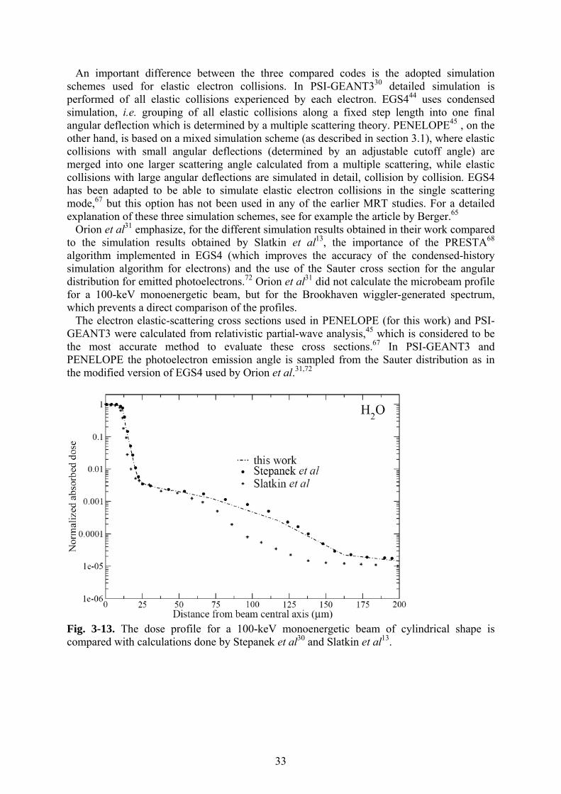
Fig. 3-12 A detailed view of the dose fall off at distances from the microbeam center which, for a composite dose distribution as used in MRT, would correspond to the distances to the dose valley. 3.8 Comparison with calculated dose profiles from earlier studies of MRT dosimetry A calculated dose profile for a 100-keV cylindrical beam is shown in Fig. 3-13, together with profiles from earlier studies of MRT by Stepanek et al30 and Slatkin et al13. Data from Stepanek et al, obtained using PSI-GEANT3, show good agreement with results obtained in this work but the dose profile from Slatkin et al, using an early version of EGS444 (without the more recent extensions to the code67-71), differs to a certain extent in the valley region, in particular between 12.5 and 200 µm, where a lower dose is predicted. The reason for this discrepancy cannot be completely determined because of the complicated interplay of interaction models and transport algorithms used in different simulation codes.
33
An important difference between the three compared codes is the adopted simulation schemes used for elastic electron collisions. In PSI-GEANT330 detailed simulation is performed of all elastic collisions experienced by each electron. EGS444 uses condensed simulation, i.e. grouping of all elastic collisions along a fixed step length into one final angular deflection which is determined by a multiple scattering theory. PENELOPE45 , on the other hand, is based on a mixed simulation scheme (as described in section 3.1), where elastic collisions with small angular deflections (determined by an adjustable cutoff angle) are merged into one larger scattering angle calculated from a multiple scattering, while elastic collisions with large angular deflections are simulated in detail, collision by collision. EGS4 has been adapted to be able to simulate elastic electron collisions in the single scattering mode,67 but this option has not been used in any of the earlier MRT studies. For a detailed explanation of these three simulation schemes, see for example the article by Berger.65 Orion et al31 emphasize, for the different simulation results obtained in their work compared to the simulation results obtained by Slatkin et al13, the importance of the PRESTA68 algorithm implemented in EGS4 (which improves the accuracy of the condensed-history simulation algorithm for electrons) and the use of the Sauter cross section for the angular distribution for emitted photoelectrons.72 Orion et al31 did not calculate the microbeam profile for a 100-keV monoenergetic beam, but for the Brookhaven wiggler-generated spectrum, which prevents a direct comparison of the profiles. The electron elastic-scattering cross sections used in PENELOPE (for this work) and PSI-GEANT3 were calculated from relativistic partial-wave analysis,45 which is considered to be the most accurate method to evaluate these cross sections.67 In PSI-GEANT3 and PENELOPE the photoelectron emission angle is sampled from the Sauter distribution as in the modified version of EGS4 used by Orion et al.31,72
Fig. 3-13. The dose profile for a 100-keV monoenergetic beam of cylindrical shape is compared with calculations done by Stepanek et al30 and Slatkin et al13.
34
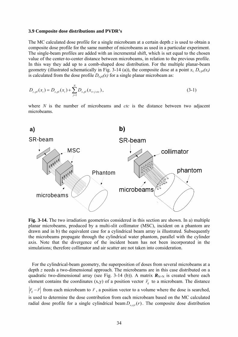
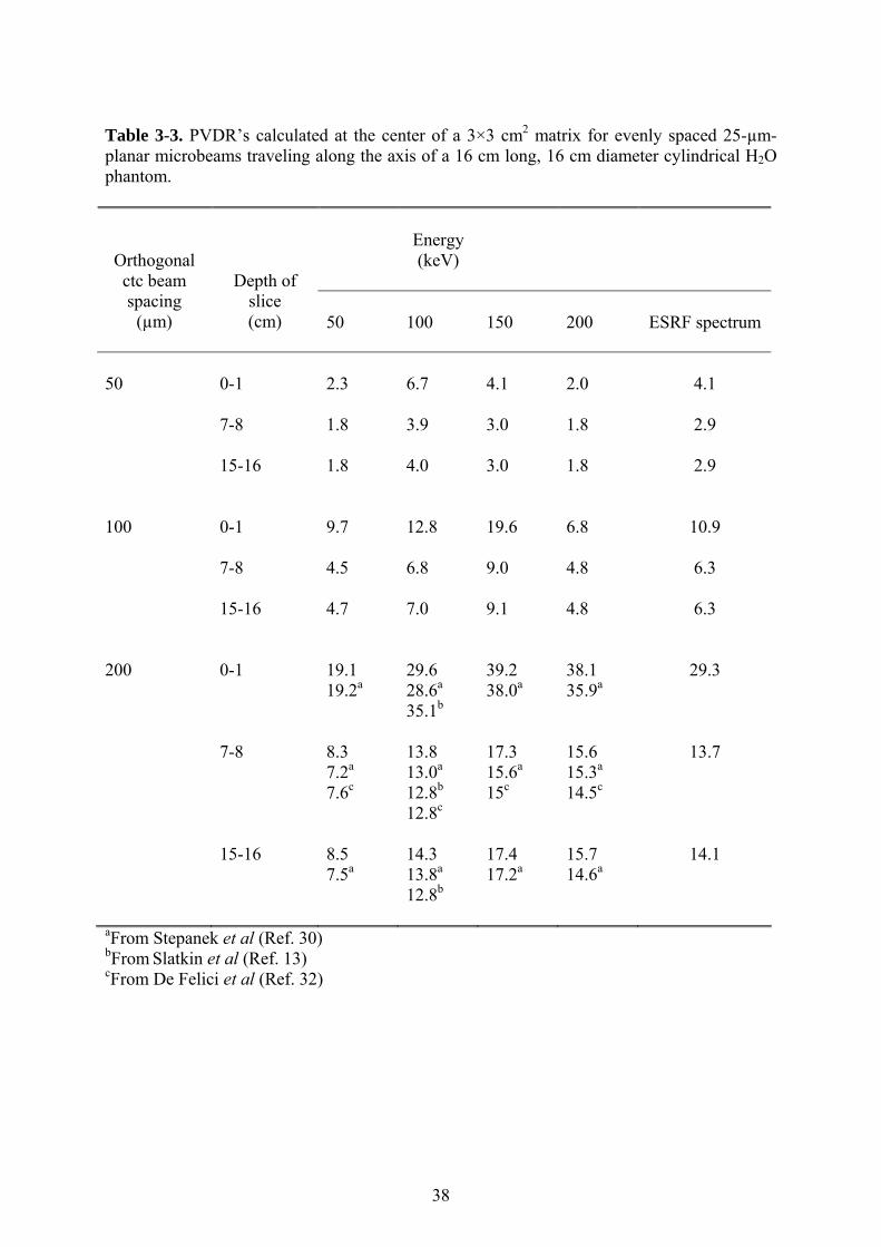
3.9 Composite dose distributions and PVDR’s The MC calculated dose profile for a single microbeam at a certain depth z is used to obtain a composite dose profile for the same number of microbeams as used in a particular experiment. The single-beam profiles are added with an incremental shift, which is set equal to the chosen value of the center-to-center distance between microbeams, in relation to the previous profile. In this way they add up to a comb-shaped dose distribution. For the multiple planar-beam geometry (illustrated schematically in Fig. 3-14 (a)), the composite dose at a point xi, Dc,pl(xi) is calculated from the dose profile Ds,pl(x) for a single planar microbeam as:
∑=
⋅++=N
jctcjiplsiplsiplc xDxDxD
1,,, )()()( , (3-1)
where N is the number of microbeams and ctc is the distance between two adjacent microbeams.
SR-beam
MSC
Phantom
microbeams
a)
Fig. 3-14. The two irradiation geometries considered in this section are shown. In a) multiple planar microbeams, produced by a multi-slit collimator (MSC), incident on a phantom are drawn and in b) the equivalent case for a cylindrical beam array is illustrated. Subsequently the microbeams propagate through the cylindrical water phantom, parallel with the cylinder axis. Note that the divergence of the incident beam has not been incorporated in the simulations; therefore collimator and air scatter are not taken into consideration. For the cylindrical-beam geometry, the superposition of doses from several microbeams at a depth z needs a two-dimensional approach. The microbeams are in this case distributed on a quadratic two-dimensional array (see Fig. 3-14 (b)). A matrix RN×N is created where each element contains the coordinates (x,y) of a position vector ijr to a microbeam. The distance
rrij − from each microbeam to r , a position vector to a volume where the dose is searched, is used to determine the dose contribution from each microbeam based on the MC calculated radial dose profile for a single cylindrical beam )(, rD cyls . The composite dose distribution
35
)(, rD cylc due to N cylindrical microbeams was finally calculated using the following equation:
∑∑= =
−=N
j
N
iijcylscylc rrDrD
1 1,, )()( . (3-2)
The PVDR’s were calculated in the middle of the microbeam arrays for the centermost peak and valley doses. PVDR’s calculated in this work are presented in Tables 3-2 and 3-3, together with values calculated in earlier studies.13,30,32 The beam sizes, phantom material and irradiation geometries used in this work were the same as used in the earlier works. Calculations were performed for four monoenergetic photon beams (50, 100, 150, and 200 keV) and for an x-ray beam with energies sampled from the measured ESRF spectrum (shown in Fig. 2-1). As shown in Tables 3-2 and 3-3, planar beams give much lower PVDR’s than the cylindrical beams. This is the consequence of the higher dose deposited by a planar beam at a certain distance from the beam center (for the same peak dose) as seen in Fig. 3-3. The values calculated for the ESRF spectrum are more similar to the results for the 100 keV beam than to the values obtained for the other monoenergetic energies. The PVDR’s are highest between 0-1 cm; then, between 7-8 cm and 15-16 cm the PVDR’s are similar. There is rather good agreement between results obtained with PSI-GEANT330 and PENELOPE45, especially for the planar-beam geometry. PVDR’s calculated with an early version of EGS413,44, are generally higher than those obtained from both PENELOPE and PSI-GEANT3 which is consistent with the graph shown in Fig. 3-13. More recent EGS4 results for planar beams obtained by De Felici et al32, taking the polarization of the x-rays into account for the Rayleigh and Compton scattering, show good agreement with PVDR’s calculated with PSI-GEANT3 and PENELOPE. This seems to indicate that when using a modern version of each MC code, the differences in the transversal dose profiles are small. Furthermore, De Felici et al found that the polarization of the x-ray photons did not change the PVDR’s in the center of the microbeam array at the depths studied. The variation of PVDR’s with depth can be interpreted with the help of Fig. 3-15. This figure shows how the peak and the valley dose are varying with depth in the center of a planar microbeam array for two different microbeam spacings (100 μm and 200 μm ctc). The irradiation geometry is the same as that used for producing Table 3-3 (a 3 × 3 cm2 array of planar beams); energies have been sampled from the ESRF spectrum and the same number of incident photons per beam area has been simulated. Normalization has been done to the maximum peak dose for the 100-μm ctc spacing. There is a dose buildup in the valley region due to scattered photons, up to a depth of about one centimeter, which is more pronounced for the 100-μm ctc spacing; the same kind of buildup was also seen in Fig. 3-1 for the wide scoring geometry. For the peak dose, the dose buildup is reached before 1 mm depth. For the 100-μm ctc microbeam spacing, there is a small additional contribution of a few percent from scattered radiation to the peak dose. The peak dose half-value depth is deeper for a microbeam in the middle of an array of microbeams (4.8 cm) than what was the case for a single microbeam in Fig. 3-1 (4.2 cm). The reason is that, with increasing depth, there is a larger contribution from scattered photons to the peak dose for a microbeam in the middle of an array of microbeams. In Fig. 3-16 (a) and (b) the variation of the PVDR’s (calculated in this work) with depth is shown for two different microbeam spacings (100 μm ctc and 200 μm ctc respectively) and for four different beam energies (50, 100, 150 keV, and the ESRF spectrum). When the ctc spacing is halved, the PVDR’s are reduced by more than a factor of two. Due to the increasing
36
valley dose, PVDR’s decrease at a rate which is faster than the decrease of peak dose (Fig. 3-1) for the first centimeter. After about 1.5 cm depth, the ratio of scattered to unscattered photons is changing at a slower rate and decreases slowly with depth, which leads to rather flat PVDR’s. The PVDR is thus higher between 0-1 cm due to relatively less scattered radiation close to the surface. For both the 100-μm- and 200-μm-ctc spacing the 150-keV beams give the highest PVDR’s. In Table 3-3, it is shown that by increasing the energy to 200 keV, PVDR’s become smaller again. This result is consistent with that obtained by Stepanek et al.30 Therefore, in order to obtain higher PVDR’s, it would be advantageous to use a harder x-ray spectrum than that presently used at the ESRF. This could be achieved by increasing the magnetic field of the wiggler or by adding additional filtration. The first of these alternatives is clearly advantageous in terms of available flux.
Fig. 3-15. The variation of peak and valley doses in the center of the planar microbeam array is shown for two different microbeam spacings. The doses were calculated for a 3 × 3 cm2 array of planar microbeams (each microbeam of size 3 cm × 25 µm). The x-ray energies were sampled from the ESRF spectrum. For most of the analyzed cases, there is a small increase in the PVDR’s at 15-16 cm depth. This is due to that there is no backscattering from below the depth where the water phantom ends. The microbeam peak dose is not changed much by the presence of a backscattering material. The photon backscattering, which is rather isotropically distributed, would mostly add to the valley dose for to geometrical reasons (the microbeam width is smaller than the width of the valley dose region). Since the nominator is the same, an increase in PVDR is caused by a smaller valley dose; this trend in the valley dose is seen already several millimeters upstream from the exit surface.
37
Table 3-2. PVDR’s calculated at the center of a 1×1 cm2 matrix of evenly spaced 25-µm-diameter cylindrical microbeams traveling along the axis of a 16-cm-long, 16-cm-diameter cylindrical H2O phantom.
Energy (keV)
Orthogonal ctc beam spacing (µm)
Depth of slice (cm)
50
100
150
ESRF spectrum
50
0-1
6.0
7.9a 24.5b
23.5
25.2a
29.6b
17.0
23.2a
29.3b
12.5
7-8 5.2
5.7a
10.5b
17.3 17.3a
18.9b
12.7 16.7a
21.7b
9.7
15-16 5.3
5.9a
7.0b
17.4 17.1a
16.1b
13.1 17.6a
18.0b
9.5
100 0-1 71.8
79.0a
126b
91.4 98.4a
133b
135 158a
190b
76.3
7-8 40.4
37.1a 44.1b
66.5 66.6a
77.2b
84.4 94.3a
114b
53.8
15-16 42.5
37.0a
28.7b
65.9 64.5a
65.1b
87.4 94.0a
96.6b
52.7
200 0-1 286
318a
513b
657 763a
834b
542 630a
826b
504
7-8 159
144a
173b
387 386a
391b
336 369a
468b
306
15-16 168
147a
111b
390 368a
337b
347 376a
396b
312
aFrom Stepanek et al (Ref. 30) bFrom Slatkin et al (Ref. 13)
38
Table 3-3. PVDR’s calculated at the center of a 3×3 cm2 matrix for evenly spaced 25-µm-planar microbeams traveling along the axis of a 16 cm long, 16 cm diameter cylindrical H2O phantom.
Energy (keV)
Orthogonal ctc beam spacing
(µm)
Depth of slice (cm)
50
100
150
200
ESRF spectrum
50
0-1
2.3
6.7
4.1
2.0
4.1
7-8 1.8
3.9 3.0 1.8 2.9
15-16
1.8 4.0 3.0 1.8 2.9
100
0-1
9.7
12.8
19.6
6.8
10.9
7-8 4.5
6.8 9.0 4.8 6.3
15-16 4.7 7.0 9.1 4.8 6.3 200
0-1
19.1 19.2a
29.6 28.6a
35.1b
39.2 38.0a
38.1 35.9a
29.3
7-8 8.3 7.2a
7.6c
13.8 13.0a
12.8b
12.8c
17.3 15.6a
15c
15.6 15.3a
14.5c
13.7
15-16 8.5 7.5a
14.3 13.8a
12.8b
17.4 17.2a
15.7 14.6a
14.1
aFrom Stepanek et al (Ref. 30) bFrom Slatkin et al (Ref. 13) cFrom De Felici et al (Ref. 32)
39
Fig. 3-16. The variation of PVDR’s with depth in water in the center of a 3 × 3 cm2 planar microbeam array (each microbeam of size 3 cm × 25 µm) is shown for two different microbeam spacings and for four different microbeam energies. In Fig. 3-17 is shown how the size of the microbeam array affects the PVDR’s for three cases: 1 × 1 cm2, 2 × 2 cm2 and 3 × 3 cm2. In agreement with findings in section 3.8, larger microbeam arrays (with microbeams of larger height) produce more scattered photons and therefore lower PVDR’s. Furthermore, if the ctc spacing remains the same, there are more microbeams in a larger array which also produce x-ray scattering.
40
Fig. 3-17. The variation of PVDR’s with depth in water is shown for three arrays of planar beams of sizes 1 cm × 25 µm, 2 cm × 25 µm and 3 cm × 25 µm. The sizes of the corresponding microbeam arrays are 1 × 1 cm2, 2 × 2 cm2, 3 × 3 cm2. A microbeam separation distance (ctc) of 200 µm was used in the superposition and the photon energies were sampled from the ESRF spectrum (Fig. 2-1). 3.10 Comparison of absorbed doses calculated with different MC codes For the research program on microbeam radiation therapy (MRT) at the ESRF and at a few other synchrotrons around the world, there is a need to determine the physical doses delivered to different tissues as accurately as possible. It is also important to document how these doses have been determined. Different MC codes have been used in the last years for different MRT related studies. A comparison of the doses calculated with different MC programs, for a few standard cases, is therefore motivated. For this comparison, the choice was made to simulate planar and cylindrical beams incident on reference dosimetry materials. In this section results will be presented for three different codes, PENELOPE45, EGS444 and MCNPX73. The data for EGS4 has been calculated by M. De Felici (ESRF) and the data for MCNPX by A. L. Hanson (BNL). First, the transversal dose profiles were calculated at different depths in a cylindrical water phantom for monochromatic cylindrical beams of three different energies. By calculating the transversal dose profiles information is also obtained about absolute doses, for a given number of primary photons incident on the phantom, calculated with each code. In the second part of the comparison, dose calculations were performed for cylindrical and planar beams impinging on a cylindrical PMMA phantom. For the planar beams, the x-ray energies have been sampled from the measured ESRF spectrum. Since this is the configuration which is used experimentally, the simulation results can be compared with measured data even though in this section no such comparison will be presented. 3.10.1 Dose calculations in water A cylindrical water phantom (density = 1.0 g/cm3) with diameter and height both equal to 20 cm was used in the first part of the comparison. The calculations were done for three monoenergetic energies, 50, 100 and 150 keV and for two different cylindrical beam
41
diameters 25 and 50 µm. Monoenergetic beams were used in order to facilitate the analysis of the calculated dose profiles and all energy cut-off values were set as low as possible. The doses were scored at three depths for the transversal dose profiles (0-1, 1-2 and 7-8 cm) and a total of 107 primary photon histories was simulated with each program. Since all figures cannot be shown in this document, a representative figure, Fig. 3-18, has been selected. It is displayed in log-log scale to clearly show the entire dose profile. As illustrated in the figure, the transversal dose profiles calculated with the different codes have similar shapes. Only the doses calculated by MCNPX seem to deviate slightly at intermediate distances from the microbeam. Since the differences between the transversal dose profiles are small, to highlight any dissimilarity, an additional calculation of dose-difference ratios (with respect to PENELOPE) was done. The result of this calculation is shown in Fig 3-19. The difference ratios (d.r.) were calculated with the following formula:
100)(
)()().(. ⋅
−= −
−PENELOPE
PENELOPEcodeMCcodeMC rDose
rDoserDoserrd (3-3)
where Dose(r)MC-code is the dose calculated at radial distance r with any of the three different MC-codes. In Fig. 3-19, it is shown that the discrepancies between the codes are largest near the beam edge where they, in the case of MCNPX, exceed 20 %. In the actual peak and further away from the beam border (distances > 200 µm) the differences are within ± 10 %. Even if the difference in this region is smaller, it is statistically significant since the precision used in the dose calculation was always better than 5 %. However, the large difference in the dose profiles calculated with PENELOPE and EGS4 (shown in Fig. 3-13) is seen to have disappeared with a more modern version of EGS4.44,68-71
Fig. 3-18. Transversal dose profiles at 7-8 cm depth in water for a 25-μm-diameter cylindrical beam. The beam energy was set to 100 keV in the simulations.
42
Fig. 3-19. The difference ratios, calculated using formula (3-3), are shown for the dose profiles in Fig. 3-18. In order to make a quantitative comparison of absolute peak doses, calculations of the dose deposited in 10-μm-wide cylinders (centered on the microbeam central axis) were done at different depths in water for a 25-μm-diameter microbeam and for three different monoenergetic x-ray energies. The results of these calculations are shown in Table 3-4. The absolute peak doses show agreement to within 10 %. At 100 keV (which is close to the average energy used for MRT at the ESRF), the agreement is even better. 3.10.2 Dose calculations in PMMA The second part of the comparison considered calculations of dose in a PMMA phantom. In addition to cylindrical monochromatic beams, the planar beam shapes (Fig. 2-1) was also used. A calculation of the variation of dose with depth in PMMA was done for the three x-ray energies also used in the first part of the comparison (50, 100 and 150 keV); the cylindrical-beam geometry with a 1-cm-diameter beamsize was used. The dose was scored in cylindrical bins of 2 mm radius and variable heights. The following bin lengths were used along the direction of increasing depth: From 0-10 mm, 1 mm ; from 10-100 mm, 10 mm and finally one extra point at 150 mm also with a 10 mm bin height. In Fig. 3-20, the depth-dose curves for a 100-keV monoenergetic beam are shown. Good agreement was obtained in the results produced by the three codes (also for the other two energies not shown here). For the planar beam geometry, the doses were scored at three depths (0-1 cm, 1-2 cm and 7-8 cm). The microbeam x-ray energies were in this case sampled from the measured ESRF spectrum. Two beam sizes were used, 25 μm × 1 cm and 50 μm × 1 cm. Doses were collected in bins in shapes of parallelepipeds over the full beam height, 1 cm and always with a 1 cm bin length along the axis of increasing depth (in the beam area the dose-scoring volume was 1 μm × 1cm × 1cm). The following bin widths were used in the direction perpendicular to the microbeam propagation: 0-50 μm: 1 μm l bin width; 50-100 μm: 10 μm bin width; 100-1000 μm: 100 μm bin width; 1000-20000 μm: 1000 μm bin width.
43
Table 3-4. Absorbed dose in gray at different depths in a water phantom for a 25-µm-diameter cylindrical microbeam. A total of 107 incident primary photons were simulated and the doses were scored in cylinders of 10 µm diameter, centered on the microbeam central-axis. PENELOPE
Fig. 3-20. Calculated depth-dose curves in PMMA for a 1-cm-diameter cylindrical beam. The simulations were done for a 100-keV monoenergetic beam. In Fig. 3-21, the excellent agreement in absorbed dose calculated with PENELOPE and EGS4 is shown for a 25 μm × 1 cm planar microbeam. Finally, computations of PVDR’s were performed (using equation (3-1)), for doses calculated with EGS4, MCNPX and PENELOPE. The PVDR’s, determined for 1 × 1 cm2 arrays of 25-µm-wide planar microbeams with a 200 μm microbeam separation are shown in Table 3-5. As shown in the table, the agreement in the calculated PVDR’s is very good. However, since the precision in the dose calculation is high (within ± 5 % in absolute dose), the small discrepancies sometimes seen in PVDR is statistical significant. In fact, the relative standard deviation for the PVDR’s is smaller than for the MC calculated dose because the relative statistical uncertainty in the valley dose is reduced after the superposition of many microbeams. Similar agreement in the PVDR’s (not shown here) were obtained also for other microbeam array configurations.
45
Fig 3-21. Calculated dose in PMMA at three different depths for 25-µm-wide planar beams. The microbeam x-ray energies have been sampled from the ESRF-measured spectrum (Fig. 2-1). Table 3-5. PVDR’s calculated with different MC codes for a 1 × 1 cm2 array of 25-µm-wide planar beams with x-ray energies sampled from the ESRF-measured spectrum (Fig. 2-1). The microbeam separation used was 200 µm. Depth (cm)
PENELOPE
EGS4
MCNPX
0-1 60 62 59 1-2 45 46 45 7-8 35 35 36 3.11 MOSFET-dosimeter simulations The MOSFET dosimetry is based on measuring the radiation-induced trapped charges in the so called gate-oxide layer which can be made very small (a fraction of a micrometer).37,74,75 The trapped charge is proportional, within certain limits, to the amount of radiation absorbed. The application of the MOSFET as a dosimeter in cm-wide broad beams was demonstrated already in 1970.37 More recently there has been an increased interest in using this detector in the dosimetry of microbeams.38 The design of the MOSFET, used for MRT dosimetry, is described in the next subsection and in Fig. 3-22. The size of the microbeams used in MRT is similar to the geometrical area of the gate oxide of the MOSFET in the plane of the silicon substrate. In order to obtain a high spatial resolution, a new approach for MRT dosimetry was recently proposed, the so called edge-on
46
orientation of the MOSFET,40 in which the sensitive volume of the MOSFET is aligned parallel with the propagation of the beam (See Fig. 3-23). In theory, with this orientation, the spatial resolution of the MOSFET is limited only by the thickness of the gate oxide. Measurements done in the edge-on mode have been successfully performed at the ESRF and at BNL.31,33,39 For this thesis work, the study of the MOSFET as an x-ray microbeam dosimeter has been divided in two parts, an experimental part and a theoretical part based on Monte Carlo simulations. The simulations are described in this section while the experimental results are presented in section 4.4.2. Parts of the work here presented has been published in Rosenfeld et al.76 The perturbation introduced by replacing the phantom material with the MOSFET detector interferes with the quality of the dose measurements. Moreover, the MOSFET has an energy-dependent response for lower x-ray energies that cannot be neglected and which has been experimentally demonstrated.77 The importance of these perturbations for the MRT dosimetry was not well known at the time of the measurements and was the main motivation for the present simulation study. MC simulations of deposited doses in the MOSFET gate oxide in previous studies has mostly dealt with broad beams (centimeter wide) in free-air geometry, or in a solid water phantom;78 the beam orientation has usually been perpendicular to the MOSFET surface ("front on"). The results obtained have agreed closely with experimental data. In a recent theoretical work on MRT dosimetry by De Felici et al32 the response of a piece of silicon (1-μm-wide) positioned in PMMA, in relation to pure PMMA was calculated; they did not incorporate the silicon substrate however, which lead to a symmetric response with respect to the microbeam. Finally they calculated and compared the PVDR’s for these two cases and found that by using a piece of silicon as the sensitive element, the PVDR’s would be higher. It was argued that this result was due to two different reasons: 1) the photon absorption coefficient for silicon is larger than the one for PMMA and 2) the electron stopping power, which is important for dose deposition by secondary electrons between microbeams, is also larger for silicon but by a relatively smaller ratio. 3.11.1 Geometry and composition of the MOSFET probe A generalized cross section of the REM TOT 500 MOSFET used in the measurements is shown in Fig. 3-22. An electron scanning microscopy photograph of the topology of that chip can be seen in Bräuer-Krisch et al33. The outermost layers, 1 and 9, represent the surrounding medium, PMMA. The following layers are shown in Fig. 3-22: 2. Encapsulant. Silica-filled black polymer of about 0.5 mm thickness. 3. Gate electrode. Aluminum electrode with thickness 1 µm. 4. Gate oxide. Thermally oxidized silicon, the sensitive dosimetric volume of the MOSFET detector. 5. Substrate. Crystalline silicon body, 0.5 mm thick. 6. Die bond. Silica-filled black polymer adhesive with a thickness of about 0.1 mm. The components are as for layer 2. 7. Tracks. Etched or printed cupper circuit tracks, plated on top with nickel and gold. Cu 17 μm, Ni 10 μm, Au 1 µm. 8. Carrier. Glass-fiber reinforced polymer carrier.
47
On each silicon chip four MOSFET’s of the type described in Fig. 3-22 are mounted. Two of the MOSFET’s have an oxide thickness of approximately 1 μm and the other two have a thickness of about 0.16 μm. The silicon body (substrate) of the MOSFET has the dimensions 500 μm × 1000 μm × 1000 μm. A filled epoxy cap covers the MOSFET chip before it is positioned in the PMMA phantom.
p+
source
thick body of n-type silicon
+ + +
p+
drain
n+
body contact
filledpolymer
filled polymer
SiO2
Al
Si
1.
2.
3.
4.
5.
6. 7.
8.
9.
Cu trackfibre -filledpolymer
sensitivevolume (4)
Fig. 3-22. The metal-oxide silicon field-effect structure employed in the current series of MOSFET dosimeters (RADFET's). 3.11.2 Simulation model For the simulations, a simplified model geometry of the MOSFET was considered. It consisted of only three components, a silicon substrate, a gate oxide (sensitive volume) and an epoxy-glue globule which acted as build-up material. These parts were assumed to reflect the most important features of the detector. In the general case, all parts of the MOSFET are important for the dose deposited in the gate oxide. However, for the x-ray energies used in MRT, the scattering from bonding wires etc can be assumed to be small. Fig. 3-23 shows two views of the MOSFET model structure when positioned in the edge-on orientation with respect to the microbeam used. The Si-substrate dimension was set to be 1 mm × 1 mm × 0.5 mm. The active volume, which is the SiO2 layer on its top surface, was given the size 270 μm × 180 μm × 1 μm. A similar but inactive layer of "field oxide (FOX)", visible in Fig. 3-23, completely surrounds the sensitive volume in the X-Z plane.
48
X-rayfield
z
x
Sensitivevolume
(1μm wide)
X-rayfield
Blackepoxy
Si body
z
y
Fig. 3-23. Simulation model of the MOSFET viewed from two angles. In the right side figure, the thickness of the sensitive layer has been exaggerated in order to make it visible. To obtain the microbeam dose profile, the scanning direction is along the Y-axis. The entire MOSFET was then considered to be embedded in a cubic PMMA phantom with a side-length of 10 cm and irradiated by a synchrotron microbeam, with a cross section of 25 μm × 500 μm. This is a beamsize which has been used in the MOSFET dosimetrical measurements. The microbeam x-ray energies were sampled from the measured spectrum at ESRF (Fig. 2-1). The MOSFET was moved after each simulation in a direction perpendicular to the direction of the beam, thereby recording the transversal dose profile. An illustration of the scanning geometry is shown in Fig. 3-24.
PMMA-phantom
microbeam
MOSFET
Fig. 3-24. MOSFET dosimeter positioned in a PMMA phantom. The scanning direction of the MOSFET has been indicated with a double arrow.
49
The PENELOPE code package was used for the Monte Carlo simulations of the MOSFET response. Since the sensitive volume of the MOSFET is very small compared to the PMMA-phantom into which it is positioned, many more interactions will take place in the phantom than in the sensitive oxide volume. When measurements at synchrotrons are performed, this is not an issue since the number of photons available is almost infinite. However, when running MC simulations this becomes an issue since the random-number generator used can only produce a random-number sequence of a limited length. When a certain number of primary photon histories have been simulated, the random number sequence repeats itself. This problem becomes particularly severe when simulating the detector response outside the direct irradiation field. In order to achieve a better precision (a smaller variance) in the estimated dose deposited in the sensitive volume, a statistical variance reduction method called splitting was used.45 The splitting method is based on multiplying the number of particles moving in regions of interest by a predetermined factor and at the same time multiplying their statistical weight w by the inverse of the same factor. Then the estimated dose D and variance 2
Dσ , for a given number of primary photon histories in the sensitive volume, can be calculated as:
∑=
⋅=N
iii dwD
1
(3-4)
( )∑=
−⋅=N
iiiD Ddw
1
222σ (3-5)
where N is the total number of interactions in the sensitive volume, wi is the weight associated with the interacting particle and di is the dose deposited in interaction i. Using the splitting technique, up to 2147483648 (the end of the random number sequence used in PENELOPE) primary photon histories were simulated for each run which took about eight hours on a Pentium 4 computer. The primary photons were assumed to start on top of the phantom with a common direction opposite to the normal of the phantom surface. 3.11.3 Simulation results Simulations of dose deposition in the MOSFET, positioned in the “edge-on” orientation, were carried out at a depth of 7 cm in the PMMA phantom. Additional simulations were performed with the MOSFET replaced by a piece of PMMA of the equivalent size. Fig. 3-25 shows the results of these simulations. Errorbars corresponding to one standard deviation are shown for the MOSFET simulations. When the MOSFET is replaced with PMMA (the solid curve) a symmetric dose profile is obtained as expected. An asymmetric peak is seen for the MOSFET simulation with a reduced dose for the side where the microbeam is incident on the epoxy globule of the detector. The fall-off of dose below the 70% dose level on the left side of the peak is in close agreement with the dose deposited in PMMA since the effective atomic numbers of PMMA and epoxy are rather similar. An increased dose is obtained far into the valley dose region when the microbeam is incident on the silicon body. More secondary electrons, from photon interactions, are generated in silicon than in epoxy. Furthermore, the electron scattering power, which determines the width of the electron angular distribution, is larger for silicon. For 100 keV electrons, the range in silicon is about 80 µm and for 200 keV it is 250 µm. This means that the range of the electrons is larger than the width of a
50
microbeam which allows them to produce a dose enhancement in the gate oxide even when the beam is only impinging on the silicon body. When the microbeam traverses the silicon body, the scattered electrons can reach the sensitive volume and produce a tail in the right-hand part of the dose response curve which is larger than for the case of pure PMMA. Also more photons are scattered from the Si body than from the equivalent piece of PMMA, even though this contribution is smaller than that from electron scattering.
Fig. 3-25. Comparison of dose deposited in a MOSFET positioned in a PMMA phantom with dose deposited in pure PMMA. The added silica powder in the epoxy cap was meant to compensate, to a certain degree, for the different scattering properties of silicon and PMMA. In order to determine the effect of this compensation on the distortion of the dose profile, the simulations for the edge-on irradiation of the MOSFET was repeated with the epoxy cap replaced with a PMMA cap of the same shape. Fig. 3-26 shows that the black epoxy is very close to PMMA in terms of the secondary-electron scattering properties for the photon spectrum used in MRT. A somewhat more symmetric response is seen in the calculated dose profile when the MOSFET is covered by an epoxy cap, in comparison with when the cap is made of PMMA; this fact suggests that the black epoxy is somewhat more similar to silicon in its scattering properties. To decrease the dose-profile asymmetry, an edge-on face-to-face paired (EOFFP) MOSFET geometry was tested in a simulation. This new kind of detector geometry is shown in Fig. 3-27. A comparison of the dose profile calculated for the EOFFP MOSFET to that calculated in pure PMMA is shown in Fig. 3-28. The EOFFP MOSFET simulation shows good agreement with the upper part of the dose profile for PMMA (both have a FWHM of 25 µm) and the dose profile is symmetric. The larger tailing (valley dose) on both sides of the dose peak is the result of more electrons scattered from within the 500-µm-wide silicon body compared to the scattering from PMMA.
51
Fig. 3-26. Comparison of simulated MOSFET-measured dose profiles when using different kinds of build-up materials (cap).
500 μm
Si Si
Sensitive Oxide
1 μm
Fig. 3-27. Geometry of the proposed EOFFP (Edge-on face-to-face paired) MOSFET.
52
Fig. 3-28. Comparison of dose profile calculated in pure PMMA and in the MOSFET, embedded in PMMA, with the new EOFFP design. 3.11.4 Discussion From the simulation results a few general observations can be made. First of all, a larger peak dose is calculated when the pure PMMA is replaced by a MOSFET detector. However, the valley dose is also higher over a large interval on one side of the microbeam (see Fig. 3-25). The calculated valley dose on the opposite side of the microbeam is somewhat smaller than in the case of pure PMMA. Further away than 100 micrometer from the center of the microbeam, the simulation results of the MOSFET response begin to be unreliable due to large statistical uncertainties; this is despite the variance reduction technique used and the fact that the random number sequence used in PENELOPE was run to the end (Any random number generator can only produce a finite sequence of random numbers). It is for the mentioned reasons not possible to determine what the MOSFET simulated PVDR’s would be. In the experimental section (chapter 4) a comparison of MOSFET measured PVDR’s with PVDR’s calculated in pure PMMA will be presented. There is an important geometric difference between dose calculations/measurements with a MOSFET compared to dose calculated in pure PMMA, illustrated in Figs. 3-29 a) and b). These figures show an experimental arrangement for the MOSFET measurement using the edge-on orientation; typical dimensions of a MRT microbeam array is shown with a microbeam separation of 200 µm and a microbeam width of 25 µm. The doses in the peaks and in the valleys are determined by a superposition of scattered particles from neighboring microbeams. When measuring the peak dose (Fig. 3-29 a)), two microbeams are simultaneously irradiating the central parts of the silicon substrate. In contrast, when measuring the valley dose (Fig. 3-29. b)), 2.5 microbeams are at the same time irradiating the detector. For the case shown in Fig. 3-29 b), the two adjacent microbeams (to the right) are also 100 µm closer to the Si-SiO2 interface. This may produce relatively large dose increments in the valley dose, reducing the experimental PVDR in comparison with the
53
PVDR’s obtained from simulations done in homogeneous PMMA. A thinner silicon body can therefore be expected to improve the symmetry of the valley dose measurement. The absolute values of the MOSFET measured dose increment in the valley dose region will also depend on the x-ray spectra of the photons. The spectrum in the valley is shifted towards lower energies compared with the spectrum in the peak, however not by much as shown in Fig. 3-8. An increase in valley dose causes a bigger change in PVDR than the equivalent change in peak dose since the valley dose is originally small and is the denominator of the PVDR ratio. To give an example, a peak dose of 100 Gy and a valley dose of 0.1 Gy produce a PVDR of 1000. Now if the peak dose is increased by 0.3 Gy the PVDR changes to 1003. On the other hand if the valley dose is increased by 0.3 Gy the PVDR is changed to 250, a factor four smaller!
54
a)
200 μm
30 μm
10 μm
200 μm
30 μm
10 μm
Si - substrate
500 μm SiO2
b)
200 μm
30 μm
10 μm
200 μm
30 μm
10 μm
Si - substrate
500 μmSiO2
Fig. 3-29. MOSFET placed in the "edge-on" dose measuring orientation inside a phantom being irradiated by a microbeam array at a) the position for a peak dose measurement and at b) the position for a valley dose measurement.
55
3.12 Treatment planning In the radiotherapy treatment planning process, the radiation doses to be administered to the patient can be calculated using different methods providing different degrees of accuracy. In hospitals, doses from x-ray beams are usually evaluated using approximate analytical calculation models.43 Occasionally, more precise Monte Carlo simulations are employed for dose calculations. However, this procedure is not yet routinely used due to the long computational times necessary. The x-ray beams normally used in radiotherapy are rather large (typically several centimeters wide) which leads to slowly varying dose distributions on the microscopic scale. A dose scoring grid with an element size of a few mm is often sufficient for the clinical dosimetry. The treatment planning systems existing in hospitals typically use image information from x-ray computerized tomography (CT) to obtain material composition data (or electron-density data). The picture elements in the images delivered by the CT-scanner are smaller than the elemental size used in the dose scoring grid. A visualization of the calculated dose distribution in two or three dimensions is often needed during the treatment plan preparation. Typically, the final plan is evaluated by studying two-dimensional isodose curves superpositioned on CT anatomical images. 3.12.1 Issues in treatment planning for MRT The treatment planning necessary for the MRT preclinical trials presents some particular difficulties. First of all the beams are much smaller than photon beams used in hospitals. This means that a very high spatial resolution, of the order of one micron, in the dose scoring grid is needed in the vicinity of the microbeam. Furthermore, the dose outside the primary radiation field, in the valley dose region, is important for the therapeutic effect of MRT. When using a conventional treatment planning system, the dose deposited outside the direct irradiation field would be considered the most inaccurate part of the calculated dose plan. There is no CT-scanner available which can provide images with 1 µm resolution, which would be needed for the description of the material composition of the irradiated body. If images from a CT scanner with a resolution of 0.5 mm are used, the information of the composition of materials traversed by a microbeam would be based on the average electron density over microscopically large areas. If the dose calculations for microbeam arrays (of the size of square centimeters) are done with micrometer resolution, a computer memory problem will also arise if 3-D information of the dose deposition is needed.†† Therefore a compromise is needed, one way or another, in the calculation-model accuracy and in the spatial resolution of the dose calculation. Simplifications in the dose calculation is possible when working with homogeneous materials; dose-scoring volume elements, with side lengths that are adapted for in which direction the variation in dose is largest, can be used. This technique has already been applied several times earlier in this chapter. In addition, symmetries of different irradiation geometries can be identified to simplify the calculations. A few examples of dose distribution calculations, when applying the mentioned simplification techniques, will be presented in remaining parts of this chapter. 3.12.2 Isodose calculations in homogeneous materials
†† For a 2-D image, with micrometer resolution, of the dose distribution produced by a 1 × 1 cm2 microbeam array, nearly one gigabyte of memory space is needed.
56
In Figs. 3-30 and 3-31 examples of two-dimensional displays of calculated dose in water are shown for single microbeams and for arrays of microbeams, respectively. The doses were calculated with one millimeter depth resolution but with a higher resolution in the transversal direction (variable binwidth, the smallest was 1 µm). Results obtained with the ESRF spectrum are compared with those obtained with 2-MeV monoenergetic x-rays. In Fig. 3-30 it is shown that the transversal dose fall-off is faster for a beam of lower x-ray energies, such as the ESRF-spectrum beam, compared to a 2-MeV x-ray beam. However the 2-MeV beam shows less attenuation with depth, a feature which is desired when treating deep-seated tumors. As it was mentioned earlier in this chapter, for a specific treatment, an appropriate beam energy has to be selected as a compromise between depth penetration and rapid lateral dose fall-off. Fig. 3-31 shows isodose curves calculated in a water phantom for incident microbeam arrays with the two x-ray beam energies shown in Fig. 3-30. The dose distributions have been obtained from a superposition of a MC calculated dose distribution for a single microbeam; ten beams were used in the superposition using the method described in section 3.9. It is evident that, in order to achieve high PVDR’s, the ESRF spectrum beam is more appropriate as beam energy than 2-MeV x rays.
57
a)
b)
Fig. 3-30 Dose distributions for x-ray microbeams incident on a water phantom. The x-ray energies have been sampled from a) the ESRF-spectrum b) a 2-MeV monoenergetic beam.
58
a)
b)
Fig. 3-31 Isodose curves produced by multiple x-ray microbeams incident on a water phantom when using a) the ESRF spectrum as beam energy and b) 2-MeV monoenergetic beams. For each case two of the isodose curves have been labeled.
59
3.12.3 Simulation of dose deposition in tissue-equivalent phantoms In the recent thesis work of Raphael Serduc6 on x-ray microbeam induced brain-vasculature damage, it was considered necessary to know the dose at various locations inside a mouse head. With this aim, dose calculations were performed with PENELOPE,45 in which the mouse brain was modeled as a cube of side length 2 cm. The brain-model was covered by a 0.5 mm bone layer and a 0.5 mm skin layer on the faces of all sides. The compositions were taken from ICRU report 44.79 The same beam height and width (5 mm × 25 µm) was used in the simulations as in the real mice irradiations. The doses were scored in a two-dimensional grid in such a way that information was obtained not only about the transversal dose variations, but also of the variation of dose with depth. As in the previous section, the dose distribution for a single microbeam was calculated and later used in a superposition. A total of 18 microbeams were used with a ctc spacing of 200 µm as in the real experiment. A depth-dose profile along the central microbeam peak was extracted and is shown in Fig. 3-32 a). The dose increment in the bone tissue is evident both on the beam entrance and exit side. The variation of the microbeam peak dose inside the brain is otherwise slow. In Fig. 3-32 b) a transversal dose profile is shown, extracted along a direction perpendicular to the microbeam propagation. This permitted the calculation of the PVDR (indicated in the figure).
60
a)
b)
Fig. 3-32 a) The depth-dose curve in the mouse head for the centermost microbeam (peak dose. b) A transversal dose profile extracted in the middle of the mouse head is shown. The PVDR has also been calculated and is indicated.
61
3.12.4 Cross-firing arrays of microbeams In the preclinical trials of MRT, different irradiation geometries have been used. One of the irradiation techniques tested was based on cross-firing two arrays of microbeams in an interlaced way (Bräuer-Krisch et al80). This geometry is illustrated in Fig. 3-33. First, the rat is irradiated with a microbeam array from one direction; the rat is then rotated 90 degrees around a rotation axis running parallel with the extension of the rat. After a small displacement along the rotation axis, corresponding to half the microbeam center-to-center (ctc) spacing, the second microbeam array is delivered. In this way only the valley doses overlap in the crossfired region.
Fig. 3-33 Two microbeam arrays are crossing each other in an interlaced way over the rat-tumor volume. In the PENELOPE MC simulations, done to determine the doses deposited with this technique, the rat head was substituted by a PMMA cylinder of radius 1 cm and length 4 cm. The simulation of the dose distribution created by one microbeam was performed, after which an arbitrary number of dose profiles can be superimposed to produce the composite dose distribution. One slit of the Archer multi-slit collimator12 was also incorporated into the simulation and the measured ESRF spectrum was used as beam energy to obtain a realistic microbeam x-ray spectrum incident on the rat phantom. The doses were scored between 9-11 mm depth which should correspond to the tumor location. Symmetry in the dose deposition was then obtained, with respect to the rotation axis, and the dose distribution could be obtained by simply adding the total number of microbeams used. Two microbeam arrays of size 8 ×8 mm2, each containing 42 microbeams with a center-to-center (ctc) spacing of 211 µm, incident perpendicularly to each other, were considered. The interlaced cross-firing technique created a microbeam ctc spacing in the tumor volume of only 105 µm. Dose distributions were calculated for the tumor-volume where there is a contribution from 84 beams and in the healthy-tissue volume, next to the tumor, were 42 beams are contributing to the composite dose. Fig. 3-34 shows the calculated dose distributions and Table 3-7 shows the valley doses obtained in the healthy and tumor volumes for certain delivered surface peak doses. The valley dose was increased by a factor of approximately three in the crossfired region.
62
Fig. 3-34 Dose distributions in the rat head resulting from a uni-directional microbeam-array exposure (solid line) and from the interlaced cross-firing technique (dashed line). Table 3-7. Summary of irradiation protocol and Monte Carlo calculated peak and valley doses. The center-to-center (ctc) spacing between microbeams is also indicated. Peak dose surface (Gy)
625
550
450
ctc
Valley dose (Gy) Healthy tissue
11.7
10.3
8.4
105 µm
Valley dose (Gy) Tumor area
34.4
30.3
24.8
211µm
63
4. EXPERIMENTAL DOSIMETRY 4.1 X-ray spectrum measurements As was mentioned in the introduction, it is of importance for both the theoretical and for the experimental dosimetry that the x-ray spectrum in the microbeams is known as precisely as possible. This knowledge will improve the accuracy of the dose calculations (which use the x-ray spectrum as input) and will also provide essential information when selecting an adequate dosimeter (concerning energy-dependent response). Periodically repeated measurements of the spectrum are necessary in order to maintain a high quality of the treatment and for patient safety reasons. Also, as is the case here, after the installation of new x-ray filters, it should be checked that there are no impurities or cracks in the filters. The x-ray spectrum generated by the wiggler and modified by a series of absorbers can be calculated using computer codes based on analytical methods.81 (The wiggler insertion device is described in Appendix A-2). The angular distributions of multiple scattered photons and the spectra of secondary electrons are more difficult to calculate analytically. For the MRT application, these distributions will be more important to know after the final collimation to microbeams; this takes place further downstream from where the spectral measurement is done. The desired distributions can be obtained in a second-step calculation starting with the measured or calculated spectra. Due to the enormously high x-ray flux from a synchrotron, a spectral measurement cannot be done directly by placing a solid state detector in the direct beam since it would be saturated. Instead, a technique called x-ray powder diffraction is used, with which the beam diffracted by a sample is detected.9 This will produce an incident x-ray flux on the detector which is orders of magnitude smaller compared with the primary beam. This technique will be briefly explained in the next subsection, preceded by an introductory section about the basics of x-ray diffraction. 4. 1. 1 X-ray diffraction In this section, a few results from the theory of x-ray diffraction will be described with the aim of introducing the experimental work presented in section 4.1.2 and 4.1.3. A more complete overview of the x-ray diffraction method can be found in one of several books on this subject.82,83 The studies of crystalline materials is one of the most important research activities at a synchrotron.9 A crystal is a solid in which the constituent atoms are packed in a regularly ordered, repeating pattern which extends in all three spatial dimensions;84 it can be modeled as a sum of discrete planes separated by a distance d. The crystal structure is composed of unit cells which are periodically repeated in three dimensions on a lattice. The unit cell is the spatial arrangement of atoms which is tiled in three-dimensional space to describe the crystal and is specified by its lattice parameters, i.e. the length of the cell edges and the angles between them. The positions of the atoms inside the unit cell are described by a set of atomic positions measured from a lattice point. When x-rays are incident on a crystal they will interact with its atoms in the different ways described in chapter 2. The photons which are coherently scattered in a crystal can, as a result of constructive interference of photons scattered from different planes, give rise to so called Bragg peaks (directions where the scattered photon intensity is high). X-rays reflected (coherently scattered) from different planes will superpose in phase if the difference in path
64
length of different x-rays is equal to an integer multiple of the x-ray wavelength. Bragg’s law gives the angles for constructive interference (but not the intensity of the Bragg peaks) for radiation scattered by a crystal:
)sin(2 θλ ⋅⋅=⋅ dn (4-1) where n, an integer number, is the order of the interference maxima; λ is the wavelength; d is the distance separating the crystal planes and θ is the angle of incidence (and of reflection) of the radiation, relative to the crystal planes. For the experiment described in the next section, an aluminum powder was used. Aluminum has a face-centered cubic (FCC) unit cell structure,84 in which there is one basis atom at each corner and in the center of each face of the unit cell. The lattice parameter a, giving the side length of the cube, is 4.05 Ångstrom.84
The d-spacing between crystal planes for a cubic lattice for a specific reflection (h,k,l) can be calculated from:
222 lkhadhkl
++= (4-2)
where h,k,l are the so called Miller indices describing families of planes. The incident angle of the x-ray and its wavelength determine, together with selection rules for Miller indices, which set of crystal planes is relevant. The Bragg law can also be written in the less familiar energy scale for a fixed angle θ:
)sin(2))sin(2/(
222
θθ
⋅⋅++⋅⋅⋅
=⋅⋅⋅⋅=a
lkhchndchnE (4-3)
where h is Planck’s constant and c is the phase velocity (in this case approximately the speed of light). With formula 4-3, the energy of Bragg peaks observed at a fixed angle can be calculated (see Fig. 4-2). In a Cartesian coordinate system, the location of a unit cell is represented by the vector R and the site of each atom is specified by the vector r with respect to a point of origin in that unit cell. The position of any atom in the crystal can then be specified as: rR + . The scattering strength of the crystal, is proportional to the square of the scattering amplitude, )(qS crystal , defined by the following expression:9
∑∑=
⋅⋅
=
⋅⋅ ⋅⋅=N
j
Rqin
i
rqii
crystal ji eeZqFqS11
),()( (4-4)
where q is the momentum transfer in the elastic photon collision; the first sum, called the unit-cell structure factor, is a sum over the n atomic form factors ),( ZqFi multiplied by the phase factor, for all n atoms building up the unit cell; the second summation is accumulating the scattering contributions for all N unit cells, and is called the lattice sum. The lattice sum has a maximum when the scalar product IRq ⋅=⋅ π2 , (I = integer) for all unit cells. The sum then becomes equal to N. Interference maxima (Bragg peaks) will then occur along certain directions and the intensity in these peaks will be proportional to N2. This proportionality indicates that “the larger the crystal, the stronger the diffraction pattern”; this is correct for very small crystal as used in protein crystallography but is no longer true for
65
large crystals (e.g. x-ray monochromators) when effects of extinction and absorption become important.83 4. 1. 2 Energy-dispersive x-ray powder diffraction Many materials cannot be grown as large single crystals. A powder sample, built up of small microcrystals with random orientations, can sometimes be obtained. Each microcrystal can in turn be considered as a single crystal. Powder diffraction is a standard technique to determine the crystal and/or unit cell structure.85 Honkimaeki et al52 have developed a fitting method, based on a prior knowledge of the powder sample properties, which can be used in the analysis of measurements taken using the so called energy-dispersive powder diffraction technique; the aim of the method is to reconstruct spectra of arbitrary broad-spectrum x-ray sources. According to Honkimaeki et al the following relation holds:
where )( hklhkl En is the integrated intensity in a specific reflection, )(0 hklEn is the incident photon flux per unit energy interval (the wanted quantity), hklE is the average energy in a specific reflection, A is an attenuation factor which includes x-ray absorption between the sample and the detector, polK is the polarization factor for coherent scattering, Ω is the solid
angle element viewed by the detector, t(E) is the effective thickness of the powder, hkld is the crystal-lattice spacing, 0r is the Thomson scattering length (or, equivalently, the classical electron radius), 0M is the number of unit cells per unit volume, hklp is the multiplicity of Bragg reflection hkl, hklF is the structure factor of the unit cell. All the above factors can be found in the literature, except )( hklhkl En which is measured and the incident flux )(0 hklEn which then can be calculated for each reflection energy (from a knowledge of the other factors). An advantage of this method is that information is obtained not only about the shape of the spectra, but also of the flux of the incident beam. Some of the coherent scattering is lost due to thermal diffuse scattering (TDS) (which occurs when x-rays are scattered by phonons in a crystal) in the crystalline powder; it is a type of inelastic scattering but the x-ray energy loss is normally small. TDS also gives contributions to the measured spectra in a measurement of the diffracted x-rays. Especially acoustic one-phonon TDS gives rise to peaks close to the positions of the Bragg peaks. Highly inelastic scattering like Compton and fluorescence, which are slowly varying with energy, are also giving contributions to the measured spectra. In the fitting method developed by Honkimaeki et al51 the contribution from inelastic photon scattering (including TDS) can be subtracted from the integrated intensity of the peaks. 4. 1. 3 Measurement setup Measurements were performed on the ID17 beamline, with the aim of determining the x-ray beam spectrum after passage through a series of filters. The measurement setup is schematically shown in Fig. 4-1. The incident beam was first of all collimated to a point-like beam by the primary slits inside the vacuum tube. An aluminum crystalline powder sample was put after the beryllium window, where the x-ray beam exits the vacuum tube, at 33
66
meters distance from the wiggler source. The angle 2θ was set to a fixed value of 13.6 degrees, which due to experimental constraints was the smallest accessible angle. A small part of the diffracted x-ray beam was accepted by the detecting slits and finally absorbed in the Germanium detector. The downstream end of detection slits were positioned at 270 cm distance (as far away as possible to reduce the importance of the background components) from the aluminum powder. Spectra were measured for energies up to 110 keV where the measurement error becomes large. To determine the spectra above 110 keV, a unification (a linking) of the measured and calculated data can be done. It is assumed that this is an adequate approach since the effect of the x-ray filters is most notable at lower x-ray energies. The x-ray filters in use can be chosen from five different bars (shown in Table 4-1), each containing x-ray filters of three different thicknesses plus a “white beam” position containing no filter. By moving the bars a certain filter can be chosen to tune the spectra of the beam. Different filter combinations are used for the different kinds of experiments performed at the medical beamline. In this work x-ray spectra were measured for the most commonly used filter settings used in MRT. Since not all measured spectra can be shown here, only a demonstration of how the method works will be presented. The example selected corresponds to the filter combination used in the MRT preclinical trials: Carbon 1.42 mm, Aluminum 0.28 mm, Aluminum 1.24 mm, Copper 0.35 and Copper 0.69 mm. The x-ray spectrum for a similar filter combination, measured during an earlier experiment, was shown in Fig. 2-1. A calibration of the multi-channel analyzer (MCA), connected to the Germanium detector, was done using a 241Am source. An MCA is needed since Bragg peaks of different energies will simultaneously be measured at the same angle of diffraction. A few test runs were done to find a measurement setting were an appropriate number of diffracted photons would be detected. The wiggler gap was successively reduced during these tests. For the smallest possible wiggler gap of 24.8 mm (the setting used in the MRT trials which produces the largest photon flux and the hardest x-ray spectrum), both the primary slits and the detecting slits (close to the Germanium detector) were set to 0.2 × 0.2 mm2. With a storage-ring current of 170 mA, spectra were collected over an integration time of two minutes. Table 4-1. The different filters on the five different filter bars are shown. The thicknesses are presented in millimeter. Five filters, one from each bar, can be used simultaneously. Filter bar 1
Filter bar 2
Filter bar 3
Filter bar 4
Filter bar 5
White beam
White beam
White beam
White beam
White beam
Carbon 1.42 Aluminum 0.28 Aluminum 0.71 Copper 0.35 Empty Carbon 1.15 Aluminum 0.54 Aluminum 1.24 Copper 1.06 Gold 0.077 Carbon 2.56 Aluminum 1.41 Aluminum 2.87 Copper 1.42 Copper 0.69 4. 1. 4 Measurement results In Fig. 4-2, the measured spectrum, for the standard filter settings, is shown. The peaks from reflections with Miller indices (h,k,l) are also indicated. The energies of these reflections have been calculated with the formula (4-3). The (1,1,1) reflection at 25.4 keV and a few other
67
reflections are not seen since x-rays of these energies have been absorbed by the chosen filters. Contributions to the spectrum from x-ray fluorescence in lead and tungsten are also indicated. The lead fluorescence is caused by absorption of the non-diffracted beam in the beam stop and the tungsten fluorescence is produced in the collimating slits.
2θ
Synchrotron storage ring
Beryllium window
X-ray beam
Crystalline powder
Beam stop
Detection slits
Germaniumdetector
Filters inside vacuum tube
Fig. 4-1. The experimental setup (not to scale) used in the powder diffraction experiment. The angle 2θ was set to 13.6 degrees and the distance from the crystalline powder to the back side of detector slit was set to 270 cm. The measured spectrum converted to the incident photon flux using formula (4-5) is shown in Fig. 4-3. A comparison with values from an earlier measurement (shown in Fig. 2-1) is also presented; the agreement is relatively good for the lower energies. The large fluctuations seen near 80 keV are due to the rather large perturbing contribution from x-ray fluorescence in lead (originating in the beam stop). In retrospect, it would have been an advantage having performed the measurement at a smaller diffraction angle. This would have reduced the uncertainties for energies above 80 keV. A larger beam stop may also improve the quality of the measurements since it would reduce the contribution from fluorescence.
68
Fig. 4-2. Measured spectrum after powder diffraction. Peaks which are due to reflections of x rays from certain planes (h,k,l) or from fluorescent x-rays are indicated. The “hill”-like shape of the spectrum below the peaks are due to phonon and Compton scattering in the powder.
Fig. 4-3. Measured powder diffraction spectrum converted to incident x-ray spectrum (formula (4-5)). A comparison is shown with results from an earlier measurement (Fig. 2-1).
69
4.2 Ionization chamber dosimetry in large homogeneous fields 4.2.1 Theory and method In radiation dosimetry of x-ray beams in the keV range, the recommendation from international protocols is to use air-filled ionization chambers (IC’s).35,86 For the x-ray spectral range produced by the wiggler source (see Fig. 2-1), an air-kerma calibration is recommended in the protocol issued by the American Association of Physicists in Medicine (AAPM).35 Some specific issues are connected to the dosimetry of the synchrotron-generated x-ray beam. Compared to the output from conventional x-ray tubes, the x-ray flux is several orders of magnitude higher.9 This has as a consequence that the charge created in the air volume of the IC will saturate the detector under normal MRT irradiation conditions. The ion recombination will also be high at these elevated dose rates. Furthermore, the vertical height of the x-ray beam (500 µm) is too small to cover the entire diameter of the IC. The IC has been calibrated in a large x-ray beam (covering the entire chamber with a certain margin) and the calibration value can only be trusted when using a similar beam geometry. Therefore, to perform the measurements in conditions that are similar to what they were during the calibration, the IC is scanned through the beam (or moved in incremental steps). This procedure is schematically shown in Fig. 4-4. The method to determine the air-kerma rate and the correction factor for ion-recombination here explained has been conceived by Paul Berkvens (ESRF). If the IC is scanned at speed v through the x-ray beam of height h, every infinitesimal volume element of the IC will be exposed during a time h/v. The air-kerma rate
in the beam •
K (Gy/s) is then directly obtained from the measured integrated air kerma K, as:
( ) ( ) ( )( )mmh
smmvGyKsGyK // ⋅=•
(4-6)
When the air-kerma rate has been determined with formula (4-6), different correction factors have to be applied. One factor (krecomb) will correct for the ion recombination which can be assumed to be important for large x-ray fluxes; the x-ray flux is in turn directly proportional to the measured air-kerma rate. Sollier et al87 reported an ion-recombination factor as high as 10 %. Normally krecomb is determined by using the experimental two-voltage method,35 but it can also be determined by using different dose rates and/or it can be determined theoretically. If the ion-recombination effect is larger than 5 %, the AAPM protocol does not recommend the two-voltage method. In this work krecomb will be estimated theoretically following Boag’s treatment of general (or volume) recombination for constant dose rates.56 The air-kerma corrected with the calculated correction factor, for different dose rates, can then be compared to verify the validity of the theoretical approach.
70
X-ray beamof height h
Aluminium centralelectrode
Scanningdirection
Ionization chamber irradiated during continuoustranslation in beam with speed v (m/s)
Diameter orheight of theionizationchamber
Fig. 4-4. Illustration of the air-kerma measurement. The cylindrical ionization chamber is scanned through the x-ray beam either with continuous translation or by using a “step and expose” approach. If the air-kerma rate K& from formula (4-6) is used in a calculation of krecomb (which is dose rate dependent), this correction factor would be overestimated. This is because, at each moment, only a fraction of the IC is irradiated by the scanned beam. Most of the electrons, creating ions in the IC air-volume, are created in the IC walls. These electrons will diffuse rather uniformly inside the IC air volume even if created in only a fraction of the total wall volume. A new “effective” kerma-rate ( effK& ), which gives the instantaneous air-kerma measured by the IC, is therefore calculated from the following formula:
( ) ( )( ) )(
)(/mmdiam
mmhmmh
smmvGyKKeff ⋅×=& (4-7)
where the factors are as defined in formula (4-6) except diam which is the diameter or height of the IC according to Figure 4-4. effK& should not be interpreted as the measured air-kerma rate in the x-ray beam though; it is only used for calculating krecomb. The following expression is finally used to calculate the ion-recombination factor:56
2
4
4.21UdKk effrecomb ⋅⋅+= & (4-8)
where U is the applied chamber potential (in Volt) and d (expressed in mm) is a parameter which depends on the geometry of the IC. The thimble-type IC has two parts, a cylindrical and a spherical. Therefore, two different geometry parameters have to be calculated. The following expressions are used to calculate d for a cylindrical and a spherical IC, respectively:
71
2
ln
1
1)(
⎟⎠⎞
⎜⎝⎛
⋅−
+⋅−= b
a
baba
badcyl (4-9) a.
⎟⎠⎞
⎜⎝⎛ ++⋅⋅−=
ab
babadspheric 1
31)( (4-9) b.
where a is the radius of the central electrode and b is the radius of the outer electrode. The total recombination factor is then calculated as a weighted average of the correction factors calculated for the two different volumes. The fractional volumes are used as weights.
sphericalrecombtot
spericalcylrecomb
tot
cyltotalrecomb k
VV
kVV
k ,,, ⋅+⋅= (4-10)
Correction factors for temperature, pressure and energy dependence are also applied. The final estimation of the air-kerma rate can thereafter be calculated from the following formula:
( ) ETPtotalrecombfinal kkksGyKsGyK ⋅⋅⋅=•
,/)/( & (4-11) where ( )sGyK /& is obtained from formula (4-6). An error in the height of the x-ray beam, or in the speed with which the IC is scanned through the beam, will lead to a random error in the air-kerma measurement. The error-propagation formula for random errors for equation (4-6) is: 88
22
22
22
hvKK shKs
vKs
KKs ⋅⎟⎟
⎠
⎞⎜⎜⎝
⎛∂∂
+⋅⎟⎟⎠
⎞⎜⎜⎝
⎛∂∂
+⋅⎟⎟⎠
⎞⎜⎜⎝
⎛∂∂
=&&&
& (4-12)
where the variables are as defined in formula (4-6) and sK, sv and sh are the random errors in each variable. 4.2.2 Measurement setup The air-kerma measurements were performed in the MRT experimental hutch. A cylindrical semiflex-tube IC from PTW, type 31002 (serial number 1134), with a sensitive air volume of 0.125 cm3 was used in the measurements. The IC was connected to a PTW UNIDOS type T10002 electrometer. A potential of 400 Volts was applied over the chamber electrodes, following the PTW recommendations. The IC used has been calibrated in air to have a conversion factor of 2.538 × 10⁸ Gy/C (PTW certification). It is specified by the manufacturer to have a cylindrical part of length 5 mm, a central electrode of radius 0.5 mm, an external electrode of radius 2.75 mm, and a diameter or height of the sensitive volume of 5.5 mm. The volume of the cylindrical part is:
72
=−⋅⋅= )05.0275.0(5.0 22πcylV 0.115 cm3
The volume of the spherical part is then:
125.0=sphericalV -0.115=0.01 cm3
The effective radii a and b, of the external and internal electrodes, of the spherical part of the IC are needed in the ion-recombination correction-factor calculation. Estimating the internal electrode radius b to be 0.2 mm, the external electrode radius a can be calculated from the following equation:
01.03
02.023
2 33
=⋅⋅
−⋅⋅ ππ a cm3
⇒ 17.0≈a cm 7.1= mm The d-value in formula (4-8) for the cylindrical and spherical parts can then be calculated according to formulas (4-9) a and b. This leads to cyld =2.5 mm and sphericd = 2.7 mm. By inserting the values for the partial volumes and the d-values into expression 4-10, the correction factor for ion recombination can be calculated as a function of the effective air-kerma:
)400
7.24.21(125.001.0)
4005.24.21(
125.0115.0
2
2
2
2
, ⋅⋅+⋅+⋅⋅+⋅= effefftotalrecomb KKk &&
The experimental setup is shown in Fig. 4-5. The IC was fixed at a distance of 34 meters from the wiggler source. A fast shutter system (made of tungsten blades), positioned in the vacuum tube transporting the beam, is used to permit short exposure times; 89 the shutter is coupled with the vertical translation of the goniometer where the IC is attached. The minimum reliable exposure time with this system is approximately 30 ms. The standard x-ray filter setting was used in the measurements (1.42 mm carbon, 1.53 mm aluminum and 1.04 mm copper). To reduce the effect of saturation and ion recombination, a pair of vertical slits is used to further collimate the beam vertically to produce a beamheight of 100 of 50 μm. Unfortunately, the relative error in the actual slit height increases when the slit opening decreases. This will then transfer to an increased uncertainty in measured air-kerma rate.
Ionizationchamber
X-rayfilters
Wiggler Fast shuttersystem
Verticalslits
Fig. 4-5. Illustration of the key elements of the experimental setup. The x-ray beam direction is indicated with arrows and the scanning direction of the ionization chamber is shown with a double arrow.
73
4.2.3 Measurement results The measurements were performed in the so called four-bunch storage-ring electron-filling mode which provides a current (~ 40 mA maximum current) that is lower than usual at the ESRF (~ 200 mA maximum current). This mode produces a lower x-ray flux than normal and makes the issues of charge-collection saturation and ion recombination less severe. 4.2.3.1 Air-kerma measurement by dynamical scanning Measurements were done by scanning the IC through the x-ray beam (as illustrated in Fig. 4-4) using two different vertical-slit heights (50 and 100 µm). The scans were done for different values of the wiggler gap. A 1-cm-wide beam was used and the IC was scanned vertically over 1 cm in order to cover its entire sensitive volume with a margin (effective beam size 1 × 1 cm2). The IC was scanned through the beam with a speed of 90 mm/s for the 100 µm vertical-slit opening and half of this speed was used for the measurement with the 50-µm vertical-slit opening. The fast shutter was open for 0.111 seconds for the scan with the 100 µm vertical-slit width and for 0.222 seconds for the 50-µm vertical-slit width. The results of the measurements, normalized for the storage ring current, are presented in Fig. 4-6. The air-kerma shown has been corrected for ion-recombination. In this case the maximum of totalrecombk , is 1.02. Corrections have also been done for temperature and pressure differences, compared with calibration conditions, (T =21°C, p = 99.68 kPa ⇒ kTP =
68.992.29332.1012.294
0
0
⋅⋅
=⋅⋅
PTPT
=1.02 ) as well as for the energy dependence of the IC specified by the
manufacturer (kE = 0.96). In Fig. 4-6 it is shown that the air-kerma rate decreases rapidly when the wiggler gap increases. Certain differences in the air-kerma rate are obtained for the two vertical-slit heights used. At 24.8 mm wiggler gap, 69 and 82 Gy/(s × mA) are obtained when using the 100 and 50-µm vertical slit heights respectively. An error analysis was done to determine the accuracy of the measured air-kerma rate. The uncertainty in measured kerma, converted from measured charge, is assumed to be small and is therefore ignored. The uncertainty in the slit height is approximately 5 micrometer and the maximum uncertainty in the speed of the goniometer vertical-translation motor is assumed to be 5 mm/s. These uncertainties are considered to be random errors. There are several additional uncertainties in the correction and calibration factors which are assumed to be negligibly small. This leads to an error estimate for the air-kerma rate measured with the 50 micron slit of:
22
22
2
005.005.0
45092.0505.0
092.0⋅⎟
⎠⎞
⎜⎝⎛ ⋅
+⋅⎟⎠⎞
⎜⎝⎛=Ks & ≈ 8.3 (Gy / (s × mA))
For the 100 micrometer slit, the error in air-kerma rate is:
22
22
2
005.01.0
90078.051.0
078.0⋅⎟
⎠⎞
⎜⎝⎛ ⋅
+⋅⎟⎠⎞
⎜⎝⎛=Ks & ≈ 5.3 (Gy / (s × mA))
74
The measurement error is largest for the smallest (50 µm) slit height. The measured values with the two different slit heights are therefore compatible since they are within their respective error margins.
Fig. 4-6. Measured air-kerma rate for different wiggler-gap sizes when scanning the ionization chamber dynamically through the beam. The measurements were done for two different vertical-slit heights. 4.2.3.2 Air-kerma measurement by multiple translations and exposures An additional measurement was done in which the IC was translated through the beam and irradiated with a “step and shoot” method. A vertical-slit-opening size (and a stepsize) of 50 µm was used when irradiating the IC. The smallest allowed wiggler gap of 24.8 mm was used in the measurements. The minimum allowed (reliable) exposure time of 0.03 seconds was used for each exposure in order to avoid problems with saturation. The result of this scan, the kerma measured in air at each step, is shown in Fig. 4-7. In the figure, normalization has been done with the storage-ring current and corrections have been applied for ion-recombination at each point (using formula 4-10). Before this normalization the profile has a slight slope from left to right due to the decrease of the storage-ring current. The maximum recombination correction factor calculated in this case was 1.03, which is well within the acceptable limits specified by the AAPM protocol.35
75
Fig. 4-7. Air kerma measured with the “step and shoot” method. The scan was done for a 50-µm high beam and the vertical-scan steplength was also 50 µm. From Fig. 4-7, it can be verified that the height (or diameter) of the active volume of the IC is 5.5 mm. The two peaks in the scan center are due to the aluminum central electrode which is 1 mm wide. If the air kerma (normalized by the exposure time and the storage ring current) measured at each scan point is integrated over all N exposure points, a measure of the average air-kerma rate per unit of storage ring current is obtained from the following expression:
∑= ×
⋅⋅⋅=×
N
i ii
TPEtotalrecombi
tCkkkGyK
mAsGyK1
,
)()(
))/((& (4-13)
where Ci is the storage ring current at the time of exposure number i and ti is the exposure time (in this case 0.03 s). The correction factors have values which are the same as for the dynamic scanning (see previous section), except totalrecombk , which is dose rate dependent. For the case shown in Fig. 4-7, the air-kerma rate is estimated to be 74 Gy/(s × mA). The main uncertainties in this measurement arise from two sources: 1) The uncertainty in exposure time which was estimated to be 2 ms (based on oscilloscope readings performed in the MOSFET experiments) and 2) The uncertainty in the vertical-slit height, estimated to be 5 microns. The uncertainty in slit height is in this case supposed to lead to an uncertainty in measured air-kerma of 10 %. The error in the steplength of the goniometer is assumed to be small as well as any uncertainty in the storage ring current (or in the correction and calibration factors). Using formula 4-12, the final error in the measured air-kerma rate was estimated to be 7.5 Gy /(s × mA).
76
4.2.3.3 Half-value layer determination It is common practice to specify the beam quality of a certain x-ray source, used for medical purposes, with a measurement of the so called half-value layer (HVL). Slabs of absorbers are inserted in the beam and the material thickness when the air kerma has fallen by 50 % is determined. For the x-ray energies of interest in this work a HVL determination with aluminum and copper slabs is recommended in the AAPM protocol.35 Results of a HVL measurement with 99.0 % pure aluminum slabs, done in the dynamical scanning mode, are shown in Fig. 4-8. The values shown are corrected for ion recombination. The aluminum HVL was found to be 16 mm. In an earlier experiment the copper HVL has been found to be 1.67 mm.87
Fig. 4-8. Air-kerma rate measured with aluminum layers of different thicknesses inserted in the beam. 4.2.4 Discussion The large effect of ion recombination in the IC, seen for high storage-ring currents, is not an issue in the so called four-bunch mode with lower currents. The differences in the measured value of the air-kerma rate that have been obtained for two different slit-sizes can be due to different reasons; the uncertainty in the actual slit height and height-uniformity is one of the most important reasons for the observed fluctuations. However, when the same vertical beam height of 50 µm was used in two measurements (in one case using the stepping and in the other the dynamic-scanning mode), a difference in the air-kerma rate was obtained (sections 4.2.3.1 and 4.2.3.2). This can be due to an exposure-time error produced by the fast shutter. Another uncertainty is the exact speed produced by the goniometer vertical-translation motor which moves the IC through the beam. The measured values of the air-kerma rate in this experiment are near the lower limit of the range of values presented by Sollier87 [80-100 Gy/ (s ×mA)].
77
4.3 Microbeam characterization Before each MRT experiment a control of the microbeam quality is done by measuring the regularity of the microbeam width and intensity. The measurements are done with an IC (not calibrated) permanently installed in air in the experimental hutch and with radiochromic films. Since the microbeams are produced by a multi-slit collimator (MSC), a short description will be given in the next subsection of the main features of this instrument. Thereafter, IC measurements of the microbeam characteristics will be presented. 4.3.1 Multi-slit collimation of microbeams Two different multi-slit collimators (MSC’s) have been used in the MRT preclinical trials, the so called Archer17 MSC (AMSC) and the Tecomet® MSC (TMSC)34. The principle of both of these MSC’s is similar and is illustrated in Fig. 4-9. These MSC’s consist of two stacks of alternating low- and high-atomic-number materials which can be translated, one relative to the other, to produce microbeams of a selected width. It is the width of the slit of the low-atomic-number material which defines the maximum microbeam width, which is obtained when the slits of the two stacks are perfectly aligned. The AMSC consists of two stacks of alternating gold and aluminum layers. It has a microbeam center-to-center (ctc) spacing of 200 µm and the aluminum slits are 50 µm wide. The TMSC is built up of two tungsten bars with built-in air slits. The ctc spacing is 400 µm and the width of the air slits is 100 µm. In the right side of Fig. 4-9, a photo of the frontal side of the TMSC is shown.
wide x-ray beam
x-ray microbeams
High density Low density
Fig. 4-9. Left side: The MSC’s in use consist of two parallel stacks with alternating high- and low-atomic-number materials. One of the stacks can be translated relative to the other one to create microbeams of different widths. Right side: A photo of the front side of the Tecomet® MSC is shown (viewed along the axis of beam propagation).
78
4.3.2 Measurements of the microbeam shapes In Fig. 4-10 an illustration of the measurement setup is shown. By scanning two tungsten blades through the microbeam array, with a micrometer-wide air-slit opening (typically 5 µm wide) between them, the microbeam shapes can be measured with a plane-parallel IC installed in the experimental hutch. The blades are positioned in air downstream from the multislit collimator but upstream with respect to the IC; they are moved with a steplength which is the same as the width of the air-slit opening. Microbeam profiles measured using the described method are presented in Fig. 4-11.
plane parallelIC
MSCx-ray beam tungstenblades
microbeams
Fig. 4-10. Schematic (not to scale) of the setup used in the microbeam characterization measurements. On the left side of Fig. 4-11 a measured profile for a single microbeam produced by the TMSC, approximately 75-μm-wide, is shown. The small increase in intensity seen on the edges of the microbeam is due to reflection of x-rays on the collimator walls or on the scanning slits. Total reflection of x-rays is seen for small incident angles (smaller than the critical angle) when crossing an interface from a less dense towards a denser medium.9
Fig. 4-11. The left-side figure shows an in-air measured profile (with a slit and an IC) for a 75-µm-wide beam. The scan to the right has been done over an entire microbeam array as used in MRT. In the right side of Fig. 4-11, the result of a microbeam scan for a 1-cm-wide microbeam array is shown. The full-width at half-maximum (FWHM) for every microbeam can be
79
extracted from the scan to determine the regularity of the microbeam widths. If the standard deviation in FWHM is considered to be too large, the alignment of the MSC can be corrected by moving (rotating or translating) one of the MSC stacks versus the second one. The microbeam scanning and the fine adjustments are normally done iteratively until microbeams of satisfactory quality have been obtained. An extensive characterization of the TMSC, in which the FWHM of 100 microbeams were determined for three nominal microbeam-width settings (30, 50 and 75 µm), has been reported by Bräuer-Krisch et al;34 it was found in that study that the TMSC produced more regular microbeams (smaller standard deviation in FWHM) than the AMSC.17 Fig. 4-11 shows the measured values of microbeam FWHM. The mean value and standard deviation for the three settings are presented in Table 4-2.
Fig. 4-12. Measured FWHM’s for microbeams produced by the Tecomet multi-slit collimator. Values are shown for three different nominal settings of the microbeam width (30, 50 and 75 µm). Table 4-2. Measured values of the FWHM (± one std) for three different nominal settings of the microbeam width. Nominal Position
4.4 X-ray microbeam dosimetry For the microbeam dosimetry, a calibrated dosimeter is put inside a phantom to take the scatter contribution and the beam attenuation into account. The key components in the setup
80
used for microbeam dosimetry are shown in Fig. 4-13. A fast-shutter system is used in order to be able to produce short exposure times and to deliver well-defined radiation doses.89 A PMMA phantom of size 10 × 10 × 10 cm3 is normally used for the dosimetry. PMMA is employed because it is built up of low-atomic-number materials similar to tissue and water (water is normally used as reference material in radiation dosimetry86) and because it is easy to handle. The phantom is positioned on the goniometer at 34 meters distance from the wiggler x-ray source. After exiting the vacuum tube (approximately 20 cm upstream from the MSC) the beam is propagating in air through the MSC and down towards the phantom into which the dosimeter is positioned.
PMMAphantom
MSCWiggler
Distance from wiggler x-ray source (meters)
33 340
Fast shutter
Fig. 4-13. The main components in the setup for x-ray microbeam dosimetry at the ID17 beamline (ESRF). The useful height of the x-ray beam, where the beam-intensity distribution can be considered to be uniform, is approximately 500 microns. The width of the x-ray beam is limited to about 25 mm. Irradiations with a larger effective beam height are performed by scanning the phantom vertically through the beam, just as is done in the preclinical experiments. The radiochromic film36 and the MOSFET dosimeter37 have been extensively tested/used at the ESRF for microbeam dosimetry but to date only MOSFET-measured results have been published.33,39 Measurements performed in this thesis work with these two dosimeters will be presented in the following subsections together with background information on each type of dosimetry. 4.4.1 Radiochromic film dosimetry Radiochromic film dosimetry is based on a polymerization reaction of a chemical active component upon radiation.36 The thin active layer is coated on a polyester film base. The non-irradiated film is transparent but turns increasingly blue upon irradiation. Gafchromic® HD-810 radiochromic dosimetry film,90 available from International Specialty Products (ISP) Technologies Inc., have been used in the film dosimetry for MRT. This film is designed for the dosimetry of high-energy photons and has been shown to have an energy-independent response above 200 keV. At 30 keV the densitometric response is only 70 % of what it is above 200 keV. Since the main part of the x-ray spectrum used for MRT (see Fig. 2-1) is below 200 keV, an error in the absolute dose measurement can be expected due to the
81
energy-dependent response of the film. However, since the spectra in these two regions are similar (see Fig. 3-8), the error in measured dose should be nearly the same in the valley as in the peak; therefore, for the determination of the PVDR’s, the energy dependence is not necessarily of great importance. The change in optical density (OD) of the Gafchromic® HD-810 film is linear with the absorbed dose from 0 Gy up to about 250 Gy.90 All films should be read along the same direction (with respect to the direction in which the sensitive layer of the film was applied) since the film response depends on the polarization of the analyzing light.36 Most densitometers produce light which is linearly polarized to some degree. By rotating the film, or turning it back to front, when positioned on the densitometer, a different OD may be measured. When comparing doses measured on different film pieces, one should be aware of variations in the thickness of the active component which may exist within the same badge since it can lead to a different densitometric response. Tests done with a slightly different film (Gafchromic® MD-55) have shown that the thickness variations are largest in a direction transversal to the direction in which the active layer was applied;35 differences in densitometric response as large as 15 %, for films cut from different parts of the same film badge, were obtained for films irradiated with the same dose. The chemical reactions in the active component of the film are continuing many hours after irradiation. After about 24 hours the color formation process has reached a plateau after which the OD changes only slowly. 4.4.1.1 Method A micro-densitometer, (U-2000 UV/Vis) which is specifically adapted for MRT dosimetry [no longer manufactured by J.L. automation, (U.K.)], is used at the ESRF to measure the OD of the films. The highest spatial resolution (nominally) achievable with this scanner is 1.25 µm. A lowest dose of approximately 25 Gy needs to be given to the film in order to distinguish the exposed region from the background reading with the microdensitometer. Since there are large differences in absolute doses within the dose distributions used for MRT, it is not possible to measure both peak and valley doses on the same film within the linear part of the dose-response curve.‡‡ Therefore, two films are exposed with different doses so that the peak and the valley doses can be measured on separate films within the linear dose-response range. Alternatively, a calibration curve can be prepared which takes the non-linear dose response of the film (for higher doses) into account. The irradiation geometry used in the film measurements is drawn in Fig. 4-14.
‡‡ For an expected PVDR of 40 (a common case), a peak dose of 1000 Gy has to be given to be able to
measure the valley dose; the peak doses would then have to be measured in the non-linear part of the dose-response curve.
82
PMMA-phantom
microbeams
radiochromic film
Fig. 4-14. Drawing of the irradiation geometry used in the radiochromic film measurements. 4.4.1.2 Results and discussion Irradiations with large homogeneous beams (of size 1×1 cm2) were done in order to obtain calibration films; the films were positioned on the phantom surface and the same scanning procedure was used as in the IC measurements (section 4.2). Since the surface dose in the homogeneous x-ray beams is considered to be known from the IC measurements, a cross calibration of the film densitometric response can be done. With the aim of obtaining information about PVDR’s, films positioned at different depths in a PMMA phantom were thereafter irradiated with arrays of x-ray microbeams. The readout of the films was done approximately 72 hours after their irradiation. An example of an OD profile measured along a line on a film is shown in Fig. 4-14. The film had been irradiated with a 1×1 cm2 microbeam array with 25-µm-wide microbeams with a center-to-center spacing of 200 µm. The film was positioned at 41 mm depth in a PMMA phantom during the irradiation and a peak dose of 8000 Gy was given. That would according to theoretical estimations have produced a valley dose of approximately 200 Gy. Unfortunately, the readings obtained with the scanner are not stable with time and repeated measurements of the same film suggested different OD’s. Differences as high as 50 % in measured OD from one reading to the next have been seen. Apart from the scanner related uncertainty, there are additional uncertainties related to using this type of film (as already discussed in section 4.4.1). Trying to present quantitative dosimetric results in this work, when the fluctuations and uncertainties are so large, does not seem meaningful. The most urgent improvement needed for the film dosimetry at the ESRF is to find a scanner which produces stable readings. One general impression obtained from many film measurements, despite the scanner fluctuations, is that the measured PVDR’s are considerably lower than those obtained from Monte Carlo calculations. A film measurement which can be done with relatively large reproducibility is the determination of the full–width at half-maximum (FWHM) of the microbeams. The film scanning is also used for determining the height of the microbeams (actually the height of the x-ray beam) which is normally nominally set to 500 µm by collimation. One issue which must be kept in mind, when measuring the widths and heights of the microbeams on the film, is
83
that the peak dose must not exceed the dose where the radiochromic film becomes non-linear in its dose response. Otherwise, if a calibration is not done, it could lead to an error in measured width.
Fig. 4-15. Measured optical density (OD) along a line on a radiochromic film. The film was irradiated with a microbeam array of 25-µm-wide, 1-cm-high microbeams with ctc spacing of 200 µm. In this case 8000 Gy was given as peak dose. In addition, radiochromic films can be used for a rapid control of the quality of the microbeams with the human eye. By making a simple visual inspection of the microbeam pattern on the film (without scanning), it can often be determined that an adjustment is needed. 4.4.2 Solid-state detector dosimetry (MOSFET) This section, which can be seen as a continuation of section 3.11, presents the experimental part of the MOSFET dosimetry done within the frame of this thesis work. The main references and the general description of the MOSFET dosimetry have been presented in section 3.11. Many groups have performed research in experimental MOSFET dosimetry.31,33,75 Two earlier experimental studies on MOSFET dosimetry for MRT can be mentioned: 1) Orion et al31, in an experiment performed at Brookhaven National Laboratory, studied the transversal dose fall-off from a single x-ray microbeam and showed good agreement with calculations done with an extended version of EGS444,68-71. 2) Brauer–Krisch et al33 (in a work done at the ESRF) measured the dose falloff with depth both in the peak and valley dose regions and finally determined PVDR’s for x-ray microbeam arrays. The MOSFET measured results were compared with doses calculated in pure PMMA. They found that the PMMA calculated PVDR’s were up to 20 % higher compared to those which could be measured with a MOSFET. The results reported in section 3.9 and 3.11 motivated further MOSFET measurements. First of all, in section 3-7, it was shown that the height of the microbeams is important for the dose deposition in between the beams (the valley dose). (In Bräuer-Krisch et al33, the beam height that had been used was not documented.) It was therefore decided to see if the difference in
84
PVDR’s, calculated for different beam sizes in pure PMMA, also could be verified with MOSFET measurements. To compare the quality of the microbeams produced by the Tecomet MSC with those produced by the Archer MSC, PVDR’s produced in a phantom by each collimator have been measured. By comparing measured and calculated PVDR’s (the calculations were done in pure PMMA for an idealized irradiation setup), it can be determined how close the measured PVDR’s (produced by both collimators) are to the calculation results. In section 3.11 it was shown that the simulated MOSFET-measured microbeam profile exhibited a certain degree of skewness (Fig. 3-25). This fact motivated the measurement of a microbeam profile in order to see if the calculation results could be experimentally verified. A measured microbeam profile has been reported also in the work of Orion et al31 but only on one side of the microbeam, not enabling to determine if any skewness is present. 4.4.2.1 Experimental setup The design of the MOSFET detector used in the measurements has been described in section 3.11.1. The signal detected, which indicates the integrated absorbed dose, is the change in threshold voltage (the drain to source voltage) induced by the radiation for a constant current of a few hundred μA. A gate bias voltage (in this experiment 15 V), which controls the signal strength, is applied during the irradiation of the MOSFET’s. As long as the current is stable within 1 nA the threshold voltage variation due to background noise will be less than 0.5 mV. Typically the variation in the current is less than 0.1 pA. The lower limit of reading on the instrument connected to the MOSFET is 1 mV. The MOSFET was positioned in the edge-on orientation (described in section 3.11) and embedded in a PMMA phantom. The phantom was then installed on the 3-axis goniometer (computer-controlled sample stage) located 1.0 meter downstream from the multi-slit collimator. The motors on the goniometer allow for 1 μm precision scans to be done. The experimental procedure is illustrated in Fig. 3-24, where it is shown how the MOSFET (positioned in a PMMA phantom) is moved in an x-ray microbeam field by translating the phantom perpendicularly to the beam direction. The MOSFET is an integrating dosimeter which saturates relatively fast when used in intense synchrotron beams. Therefore, the dosimetry was performed at low synchrotron storage-ring current (in the “four-bunch mode” filling of the ESRF storage ring, max current ~ 40 mA), which is proportional to the x-ray flux, to permit a larger number of measurements to be performed with a single MOSFET. After about 1000 Gy of accumulated absorbed dose the dosimeter becomes saturated and has to be replaced. The alignment of the MOSFET with respect to the x-ray microbeams was done by putting the device on the crossing point of three lasers lines which earlier had been centered on the uncollimated beam. Then the MOSFET was scanned in the vertical direction in the uncollimated x-ray beam (using a large wiggler gap not to deliver to high doses to the sensitive volume) to find the vertical center position of the beam, after which the MSC (either the Archer or the Tecomet) was inserted in the beam. Thereafter, a scan was done in the horizontal plane to find a microbeam. On the silicon chip used there is more than one gate oxide, of the type shown in Fig. 3-22, which can act as sensitive volume. Two different oxides can then be scanned simultaneously in the beam. By finding the orientation where they both show a maximum in measured dose, the extension of the MOSFET sensitive volumes can be optimally aligned with the beam; this is an important step for finding the orientation where the MOSFET has its highest spatial resolution. When the MOSFET had been aligned and the position of the centermost peak had been found, the wiggler gap was set to 24.8 mm which is the standard setting in the MRT preclinical trials. A fast shutter system is used to adjust the
85
dose given to the phantom.89 Data acquisition is performed either in stationary mode or by scanning the detector through the beam. The scanning option makes it possible to deliver smaller doses. If not explicitly stated in the text, the measurements have been performed in the stationary mode. Exact opening times of the fast shutter were measured with a photodiode, connected to an oscilloscope, at the end of the beam path. A difficult part of the measurement is to place the MOSFET exactly on the position of a peak dose produced by the small microbeams. To make sure that a reasonable peak dose is measured, checks are done against measurements in a larger (1×1 cm2) field size where any positioning error naturally is irrelevant for the reading. The relationship between the microbeam peak dose and the dose in a larger (cm-wide) field size in PMMA is well known from Monte Carlo simulations. Approximately the same relations are expected to hold also for the MOSFET measurements. The dose gradients in the valley dose region are much smaller so these measurements are not expected to show large position-dependent fluctuations over small distances. 4.4.2.2 Results 4.4.2.2.1 Cross-calibration of the MOSFET First of all, a calibration of the dose response of the MOSFET was done. The ionization chamber measured air-kerma rate for a homogeneous beam of size (1 × 1 cm2) and Monte Carlo calculated depth dose curves in pure PMMA were used as reference values in a cross calibration of the MOSFET. The calibration measurements were done at three different depths, using the homogeneous beam, to take into account the hardening of the x-ray spectrum with depth. Since silicon is of higher atomic number than PMMA, a correction for the beam hardening was considered necessary. The calibration measurements were performed for two x-ray beam qualities; in one case with the standard filter settings and for a second case with the same settings plus an additional Al-filtration of 16 mm; the latter was done since the Archer MSC has 16 mm extra of aluminum filtration compared with the Tecomet® MSC. The MC calculated percentage depth-dose (PDD) values and the calibration measurements are shown in Table 4-3. The MC calculated depth dose curve is not affected by the extra aluminum filtration. As was shown in section 4.2, 16 mm of aluminum corresponds to the dose half-value layer (HVL) for the standard filter settings. The measured calibration data show that the change in threshold voltage, to detect the same dose, is about 5 mV smaller at all depths when the extra aluminum filtration is used. This is the result of the decreased sensitivity of silicon when the x-ray spectrum is shifted towards higher energies. By comparing the calibration data for different depths and radiation qualities, it is clear that the beam hardening produced by the extra aluminum filtration is more important than the change in x-ray spectrum with depth in the PMMA phantom. Since the sensitivity of the MOSFET slowly drops off as the integrated absorbed dose increases, the linearity of the dose response was repeatedly checked during the measurements.
86
TABLE 4-3. MOSFET calibration data in (mV/Gy) at three different depths are shown for the two radiation qualities considered. Monte Carlo calculated percentage depth dose data (PDD), used in the calibration, are also shown. Depth in PMMA (mm)
PDD (no Al) %
mV/Gy (no Al)
PDD (16 mm Al) %
mV/Gy (16 mm Al)
8
92
36.7
92
30.0
28
65
37.4
65
29.8
68
31
35.6
31
28.0
4.4.2.2.2 Transversal dose-profile The measured transversal dose profile produced by a single 40-µm-wide microbeam (collimated by the Tecomet® collimator), when using a 5 micron step size, was measured. The result of this scan, where an asymmetry of the measured transversal dose profile can be observed, is shown in Fig. 4-16. A similar shape was also observed for the MC simulated dose profile shown in Fig. 3-25. In section 3.11 it was demonstrated that this shape is related to the asymmetric orientation of the MOSFET with respect to the direction of propagation of the microbeam. The calculation has not been directly compared (in the same figure) with the measurement, since the microbeam widths are different.
Fig. 4-16. MOSFET-measured dose profile for a 40-µm-wide (FWHM) beam in a PMMA-phantom. Similar to what was found for the simulated dose profile (Fig. 3-25), an asymmetry is obtained in the measured dose profile.
87
4.4.2.2.3 PVDR’s A series of PVDR’s were measured when using both the Archer and the Tecomet® MSC’s. An uncollimated beam of constant width of 1 cm was illuminating the MSC’s. Consequently, 50 microbeams were produced when the Archer MSC was used and 25 microbeams were created when the Tecomet® MSC was illuminated. The beamheight was collimated to 500 μm. The microbeam separation distance used in the measurements was 400 and 200 μm for the Tecomet® MSC and Archer MSC respectively. A smaller separation between the microbeams can be obtained by moving the MSC and irradiating again while keeping fixed the MOSFET. The measurements were done at three different depths and for different microbeam widths. PVDR’s were obtained by measuring the centermost peak and valley doses. Dose calculations were done in pure PMMA, using the same microbeam array parameters as in the measurements. Both data sets are shown in Table 4-4. The PVDR’s measured in PMMA are a factor two or more different from the calculations. This difference is much larger than what was reported by Brauer-Krisch et al33 Since the peak doses were calibrated to reproduce the depth dose curve calculated in PMMA, the reason why the measured PVDR’s are lower is that the valley dose is higher than that calculated; this may be due to a relatively small increase in valley dose as it was explained in section 3.11.4. There can be two reasons for why the measured valley dose is higher than the calculated. First of all there is a perturbation on the irradiation field, including generated secondary particles, caused by the presence of the MOSFET dosimeter. Secondly, the calculations did not consider the scattering before the phantom and all photons are assumed to start on its surface with a common direction. Any change from this ideal situation used in the simulations will lead to a higher valley dose and a lower PVDR.
88
TABLE 4-4. Comparison between PVDR’s measured with a MOSFET and PVDR’s obtained from MC simulations in PMMA. The measured data are for microbeams collimated by the Tecomet® MSC (for three different beamwidths) and by the Archer MSC (for one beamwidth). The Tecomet® collimator has a ctc spacing of 400 µm while the Archer MSC has a ctc spacing of 200 µm.
Measured values (bold fonts) and calculated values (italic fonts). It can also be noted that, when using the Archer collimator, the measured data are differing from the calculated PVDR’s by a factor of approximately three; when using the Tecomet® collimator the measured data are differing by a factor of two from the calculated data. It has been shown that the TMSC produces microbeams with more uniform widths. The importance of this beam uniformity for the PVDR’s is however unclear. In order to determine the importance of the microbeam height for the size of PVDR’s, measurements were performed for 1-cm-high microbeams collimated by the Tecomet® collimator. The results of these measurements are shown in Table 4-5 together with calculated PVDR’s. Both the measured and the calculated PVDR’s become smaller if the microbeam height is increased. The measured PVDR’s are again smaller than the calculated, but by a smaller fraction. The decrease in measured PVDR (compared with values shown in Table 4-4) is caused by an increasing valley dose at the same time as the peak dose is rather unaffected by scattered radiation. One reason for the better agreement obtained is that if the valley dose is initially higher, an extra contribution in valley dose will lead to a smaller change in the PVDR’s.
89
TABLE 4-5. Comparison between PVDR's measured with a MOSFET and PVDR’s obtained from MC simulations in PMMA. The measured data are for microbeams collimated by the Tecomet® MSC for three different microbeam widths and of constant height 1 cm.
Microbeam width (μm)
Depth in PMMA (mm)
25
50
75
8
73 116
41 62
31 43
28
68 87
34 49
22 33
68
60 80
32 43
21 30
Measured values (bold fonts) and calculated values (italic fonts).
90
5. SUMMARY 5.1 Theoretical dosimetry A detailed analysis of the microbeam dose deposition from a single microbeam has been presented. The dose deposition in water for the x-ray spectrum used for MRT is mainly due to Compton scattering. The photoelectric effect remains important for the dose deposited furthest away from the microbeam, since the fraction of the photon energy transferred to atomic electrons in Compton collisions is getting smaller the lower the incident photon energy. The deposited dose caused by electrons scattered from inside the primary microbeam field is decreasing rapidly with the distance from the microbeam. The photon-scatter contribution to the microbeam dose deposition is varying only slowly over large distances. The x-ray spectrum present in between microbeams exhibits a small shift towards lower energies compared with the incident spectrum. The microbeam peak dose has its maximum at the phantom surface and decreases exponentially with depth due to attenuation of the beam. If the dose from a larger (cm-wide) beam is measured, a somewhat different depth-dose curve is obtained due to different contributions from scattered photons. The difference in maximum peak dose for different microbeam widths can be as large as 15 % because of different degrees of charged-particle equilibrium. The peak-to-valley dose ratio (PVDR), of importance for the therapeutic effect of the treatment, is decreasing with depth. The dose in between the microbeams, the so called valley dose, is increasing with depth and reaches a maximum first after a depth of about one centimeter. When the microbeam array is getting closer to the exit surface of the phantom, the PVDR’s increase again; this is due to a decreasing valley dose which in turn is caused by a decreasing contribution from backscattered x-rays. The larger the microbeam-array size, the larger the dose in between the microbeams (the valley dose) and consequently the lower the PVDR’s. For the microbeam-array configurations tested in the preclinical trials, a mean energy of about 150 keV seems to be optimal in terms of depth penetration and high PVDR’s. Rather good agreement (generally within 10 %) is seen in a comparison of dosimetric results obtained with different modern MC codes. The dose measured with a MOSFET-dosimeter irradiated by an x-ray microbeam has been simulated. An asymmetric transversal dose profile was calculated. A treatment-planning system for MRT has to overcome several difficulties mainly related to the small size of the microbeams. Certain simplifications and the use of symmetries can increase the speed of the dose calculation considerably. Examples of treatment plans, both in homogeneous water phantoms and in animal phantoms with realistic material compositions, have been presented in this work. The dose deposition is strongly enhanced in bone for the x-ray spectrum presently used for MRT. 5.2 Experimental dosimetry X-ray spectra have been measured with the so called powder diffraction technique and reasonable agreement was seen with results from an earlier measurement. The dose in air (or more correctly the air kerma) was measured with a thimble-type ionization chamber in the uncollimated beam using two different approaches. The air-kerma rate in the uncollimated beam was measured to be 75 ± 10 Gy/(s × mA) which is near the lower limit of the range of values measured in earlier studies. The large correction factor for
91
the ion recombination, seen in earlier measurements, was found not to be a serious issue when measuring at a lower dose rate (corresponding to the four-bunch storage-ring filling mode). The aluminum half-value layer, for the standard x-ray filter settings used for MRT, was measured to be 16 mm. The film dosimetry is useful for rapid qualitative dose measurements. Presently, there are problems with the reproducibility in optical-density readings of the radiochromic film and therefore also in the dose measurements. The dose inside and near an x-ray microbeam has been measured with a MOSFET. An asymmetric transversal dose profile was obtained just as in the simulations. It was experimentally verified that the microbeam height is important for the PVDR’s. The MOSFET measured PVDR’s in PMMA are lower than the ones calculated in pure PMMA without the presence of a detector. This was concluded to be caused partly by the perturbation on the radiation field caused by the MOSFET detector itself and partly by the imperfections of the calculation model. The agreement between calculations and measurements becomes better when microbeams of larger height (one cm compared to 500 μm) are used.
92
ACKNOWLEDGMENTS I would like to thank my supervisor at the TUM, Prof. Dr. H. G. Paretzke for adopting me as a thesis student and for fruitful discussions. I would also like to thank my supervisors at the ESRF, Alberto Bravin and Elke Brauer as well as the other staff at the ESRF (and users) involved in the microbeam radiation therapy project such as: Daniel N. Slatkin, Jean A. Laissue, Herwig Requardt, Jiri Stepanek, Geraldine le Duc, Pierrick Regnard, Christian Nemoz, Michael Lerch, Anatoly Rozenfeld, Marina Defelici, Raphael Serduc, Elisabeth Schultke, Hans Blattman and Boudewijn van der Zanden. In particular I would like to thank Daniel N. Slatkin (USA) and Jean A. Laissue (Switzerland) for explaining the medical/biological effects of microbeam radiation therapy. Veijo Honkimäki and Manuel Sanchez del Rio at the ESRF are acknowledged for the help they provided in the spectral measurements/calculations. I would also like to thank the Director of studies at the Stockholm University, Bo Nilsson for his pedagogic lectures in dosimetry and Prof. José-Maria Fernández Varea at the University of Barcelona for introducing me into the field of Monte Carlo simulations of radiation transport. The department of Hospital Physics at the Karolinska Hospital in Stockholm is also acknowledged for supporting me during the time of my thesis work.
93
REFERENCES 1W. K. Röntgen, “Über eine neue Art von Strahlen (Vorläufige Mitteilung),“ Sitzungsber. Physik. Med. Ges. Würzburg, 132–141 (1895). 2aA. Köhler, “Une nouvelle méthode permettant de faire agir, dans la profondeur des tissus, de hautes doses de rayons Roentgen et un moyen nouveau de protection contre les radiodermites,” Annales d'Electrobiologie et de Radiologie 10, 661-664 (1909). 2bA. Köhler, “Zur Röntgentiefentherapie mit Massendosen,“ Münchener medizinische Wochenschrift 56, 2314-2316 (1909). 3M. Mohiuddin, M. Fujita, W. F. Regine, A. S. Megooni, G. S. Ibbott, and M. M. Ahmed, “High-dose spatially-fractionated radiation (GRID): a new paradigm in the management of advanced cancers,” Int. J. Radiat. Oncol. Biol. Phys. 45, 721-727 (1999).
4H. J. Curtis, “The use of a deuteron microbeam for simulating the biological effects of heavy cosmic-ray particles,” in Space Radiation Biology, edited by P. E. Schambra, G. E. Stapleton, and N. E. Barr. Radiat. Res. Suppl. 7, 250-257 (1967). 5H. J. Curtis, “The interpretation of microbeam experiments for manned space flight,” in Space Radiation Biology, edited by P. E. Schambra, G. E. Stapleton, and N. E. Barr. Radiat. Res. Suppl. 7, 258-264 (1967).
6R. Serduc ”Effets de la radiothérapie par microfaisceaux synchrotron sur la micro-vascularisation cérébrale saine et tumorale chez la souris,” Doctoral thesis, Univ. Joseph Fourier, (Grenoble, France) (2006).
7F. A. Dilmanian, Z. Zhong, T. Bacarian, H. Benveniste, P. Romanelli, R. L. Wang, J. Welwart, T. Yuasa, E. M. Rosen, and D. J. Anschel, ”Interlaced x-ray microplanar beams: A radiosurgery approach with clinical potential,” Proc. Natl. Acad. Sci. U.S.A. 103, 9709-9714 (2006). 8W. E. Straile and H. B. Chase, “The use of elongate microbeams of x-rays for simulating the effects of cosmic rays on tissues: A study of wound healing and hair follicle regeneration,” Radiat. Res. 18, 65-75 (1963). 9J. Als-Nielsen and D. McMorrow, Elements of Modern X-Ray Physics, (John Wiley & Sons, Inc, NY, USA) (2001). 10F. R. Elder, A. M. Gurewitsch, R. V. Langmuir, and H. C. Pollock, “Radiation from Electrons in a Synchrotron,” Phys. Rev. 71, 829-830 (1947).
11W. Thomlinson, “Medical applications of synchrotron radiation,” Nucl. Instrum. Meth. Phys. Res. A 319, 295-304 (1992).
12D. N. Slatkin, “Feasibility study for microbeam radiation therapy with 30-90 keV X rays from the NSLS X17 beamline,” in Laboratory Directed Research & Development Program,
94
Annual Report to the Department of Energy. edited by G. J. Ogeka, pp 36-37 (BNL-52320, December 1, 1991; Brookhaven National Laboratory, Upton, New York, USA). 13D. N. Slatkin, P. Spanne, F. A. Dilmanian, and M. Sandborg, “Microbeam radiation therapy,” Med. Phys. 19, 1395-1400 (1992). 14J. A. Laissue, G. Geiser, P. O. Spanne, F. A. Dilmanian, J.-O. Gebbers, M. Geiser, X. Y. Wu, M. S. Makar,, P. L. Micca, M. M. Nawrocky, D. D. Joel, and D. N. Slatkin, “Neuropathology of ablation of rat gliosarcomas and contiguous-brain tissues using a microplanar beam of synchrotron-wiggler-generated x-rays,” Int. J. Cancer 78, 654-660 (1998). 15J. M. Ordy, H. W. Barnes, T. Samorajski, H. J. Curtis, L. Wolin, and W. Zeman, “Pathological and behavioral changes in mice after deuteron irradiation of the central nervous system,” Radiat. Res. 18, 31-45 (1963). 16D. N. Slatkin, F. A. Dilmanian, M. M. Nawrocky, P. Spanne, J.-O. Gebbers, D. W. Archer, and J. A. Laissue, ”Design of a multislit variable width collimator for microplanar beam radiotherapy,” Rev. Sci. Instrum. 66, 1459-1460 (1995). 17D. W. Archer, U. S. Patent No. 5771270, 23 June (1998). 18D. N. Slatkin, P. O. Spanne, F. A. Dilmanian, J. O. Gebbers, and J. A. Laissue, “Subacute neuropathological effects of microplanar beams of X-rays from a synchrotron wiggler,” Proc. Natl. Acad. Sci. U.S.A. 92, 8783-8787 (1995). 19J. A. Laissue, N. Lyubimova, H. P. Wagner, D. W. Archer, D. N. Slatkin, M. Di Michiel, C. Nemoz, M. Renier, E. Brauer, P. O. Spanne, J. O. Gebbers, K. Dixon, and H. Blattman, “Microbeam radiation therapy,” Proc. SPIE 3770, 38-45 (1999). 20F. A. Dilmanian, G. M. Morris, G. Le Duc, X. Huang, B. Ren, T. Bacarian., J. C. Allen, J. Kalef-Ezra, I. Orion, E. M. Rosen, T. Sandhu, P. Sathé, X. Y. Wu, Z. Zhong, and H. L. Shivaprasad, “Response of avian embryonic brain to spatially segmented X-ray microbeams,” Cell. Mol. Biol. 47, 485-494 (2001). 21J. A. Laissue, H. Blattmann, M. Di Michiel, D. N. Slatkin, N. Lyubimova, R. Guzman, W. Zimmermann, T. Bley, P. Kircher, R. Stettler, R. Fatzer, A. Jaggy , H. M. Smilowitz, E. Brauer, A. Bravin, G. Le Duc, C. Nemoz, M. Renier, W. Thomlinson, J. Stepanek and H. Wagner, “The Weanling Piglet Cerebellum: A Surrogate for Tolerance to MRT (Microbeam Radiation Therapy) in Pediatric Neuro-Oncology,” Proc. SPIE, 4508, 65-73 (2001).
22F. A. Dilmanian, T. M. Button, G. Le Duc, N. Zhong, L. A. Pena, J. A. L. Smith, S. R. Martinez, T. Bacarian, J. Tammam, B. Ren, P. M. Farmer, J. Kalef-Ezra, P. L. Micca, M. M. Nawrocky, J. A. Niederer, F. P. Recksiek, A. Fuchs, and E. M. Rosen, ”Response of rat intracranial 9L gliosarcoma to microbeam radiation therapy” Neuro-Oncol. 4, 26-38 (2002). 23F. A. Dilmanian, G. M. Morris, N. Zhong, T. Bacarian, J. F. Hainfeld, J. Kalef-Ezra, L. J. Brewington, J. Tammam, and E. M. Rosen, ”Murine EMT-6 carcinoma: High therapeutic efficacy of microbeam radiation therapy,” Radiat. Res. 159, 632-641, (2003).
95
24N. Zhong, G. M. Morris, T. Bacarian, E. M. Rosen, and F. A. Dilmanian ”Response of rat skin to high-dose unidirectional X-ray microbearns: A histological study,” Radiat. Res. 160,133-142 (2003). 25M. Miura, H. Blattmann, E. Brauer-Krisch, A. Bravin, A. L. Hanson, M. M. Nawrocky, P. L. Micca, D. N. Slatkin, and J. A. Laissue, ”Radiosurgical palliation of aggressive murine SCCVII squamous cell carcinomas using synchrotron-generated X-ray microbeams,” Br. J. Radiol. 79, 71-75 (2006). 26R. Serduc, P. Verant, J. C. Vial, R. Farion, L. Rocas, C. Remy, T. Fadlallah, E. Brauer, A. Bravin, J. Laissue, H. Blattmann, and B. Van der Sanden , ”In vivo two-photon microscopy study of short-term effects of microbeam irradiation on normal mouse brain microvasculature,” Int. J. Rad. Oncol. Biol. Phys. 64, 1519-1527 (2006 ). 27H. M. Smilowitz, H. Blattmann, E. Brauer-Krisch, A. Bravin, M. Di Michiel, , J.-O. Gebbers, A. L. Hanson, N. Lyubimova, D. N. Slatkin, J. Stepanek, and J. A. Laissue, ”Synergy of gene-mediated immunoprophylaxis and microbeam radiation therapy for advanced intracerebral rat 9L gliosarcomas” J. Neuro-Oncol. 78, 135-143 (2006). 28H. Blattmann, J.-O. Gebbers, E. Brauer-Krisch, A. Bravin, G. Le Duc, W. Burkard, M. Di Michiel, V. Djonov, D. N. Slatkin, J. Stepanek, and J. A. Laissue, “Applications of synchrotron X-rays to radiotherapy,” Nucl. Instrum. Meth. A 548, 17-22 (2005). 29F. Z. Company and B. J. Allen, ”Calculation of microplanar beam dose profiles in a tissue/ lung/tissue phantom,” Phys. Med. Biol. 43, 2491-2501 (1998). 30 J. Stepanek, H. Blattman, J. A. Laissue, N. Lyubimova, M. De Michiel, and D. N. Slatkin, ”Physics study of microbeam radiation therapy with PSI-version of Monte Carlo code GEANT as a new computational tool,” Med. Phys. 27, 1664-1675 (2000). 31 I. Orion, A. B. Rosenfeld, F. A. Dilmanian, F. Telang, B. Ren, and Y. Namito, “Monte Carlo simulation of dose distributions from a synchrotron-produced microplanar beam array using the EGS4 code system,” Phys. Med. Biol. 45, 2497-2508 (2000). 32M. De Felici, R. Felici, M. Sanchez del Rio, C. Ferrero, T. Bacarian, and F. A. Dilmanian, ”Dose distribution from x-ray microbeam arrays applied to radiation therapy: An EGS4 Monte Carlo study,” Med. Phys. 32, 2455-2463 (2005). 33 E. Bräuer-Krisch, A. Bravin, M. Lerch, A. Rosenfeld, J. Stepanek, M. Di Michiel, and J. A. Laissue, “MOSFET dosimetry for microbeam radiation therapy at the European Synchrotron Radiation Facility,” Med. Phys. 30, 583-589 (2003). 34E. Bräuer-Krisch, A. Bravin, L. Zhang, E. A. Siegbahn, J. Stepanek, H. Blattmann, D. N. Slatkin, J.-O. Gebbers, M. Jasmin, and J. A. Laissue, “Characterization of a tungsten/gas multislit collimator for microbeam radiation therapy at the European Synchrotron Radiation Facility,” Rev. Sci. Instrum. 76, 064303 (2005). 35C.-M. Ma, C. W. Coffey, L. A. DeWerd, C. Liu, R. Nath, S. M. Seltzer, and J. P. Seuntjens, ”AAPM protocol for 40-300 kV x-ray beam dosimetry in radiotherapy and radiobiology,” Med. Phys. 28, 868-893, (2001).
96
36A. Niroomand-Rad, C. R. Blackwell, B. M. Coursey, K. P. Gall, J. M. Galvin, W. L. McLaughlin, A. S. Meigooni, R. Nath, J. E. Rodgers, and C. G. Soares, “Radiochromic film dosimetry: Recommendations of AAPM Radiation Therapy Committee Task Group 55,” Med. Phys. 25, 2093-2115 (1998).
37W. J. Poch and A. G. Holmes-Siedle, “The mosimeter - a new instrument for measuring radiation dose”, RCA Engineer 16, 56-59 (1970). 38A. Rosenfeld, G. Kaplan, B. Allen, F. A. Dilmanian., T. Kron, A. Holmes-Siedle “MOSFET Dosimetry of X-ray Microbeams” , IEEE Trans. Nucl Sci. 46, 1774-1780 (1999).
39A. B. Rosenfeld, M. L. F. Lerch , T. Kron, E. Brauer-Krisch, A. Bravin, A. Holmes-Siedle, “Feasibility study of on-line, high spatial resolution MOSFET dosimetry in static and pulsed X-ray radiation fields”, IEEE Trans. Nucl. Sci. 48, 2061-2068 (2001).
40G. I. Kaplan, A. B. Rosenfeld, B. J. Allen, J. T. Both, M. G. Carolan, and A. Holmes-Siedle, “Improved spatial resolution by MOSFET dosimetry of an x-ray microbeam,” Med. Phys. 27, 239-244 (2000).
41R. R. Wilson, “Monte Carlo study of shower production,” Phys. Rev. 86, 261-269 (1952). 42D. W. O. Rogers, ”Fifty years of Monte Carlo simulations for medical physics” Phys. Med. Biol. 51, R287-R301 (2006).
43A. Ahnesjö, and M. Aspradakis, “Dose calculations for external photon beams in radiotherapy,” Phys. Med. Biol. 44, R99-R155 (1999). 44W. R. Nelson, H. Hirayama, and D. W. O. Rogers, “The EGS4 code system,” SLAC report 265, (1985). 45F. Salvat, J. M. Fernández-Varea, and J. Sempau, PENELOPE, a Code System for Monte Carlo Simulation of Electron and Photon Transport, (OECD Nuclear Energy Agency, Issy-les-Moulineaux France, 2003). 46J. Sempau, A. Sanchez-Reyes, F. Salvat, H. O. ben Tahar, S. B. Jiang, J. M. Fernández-Varea, “Monte Carlo simulation of electron beams from an accelerator head using PENELOPE,” Phys. Med. Biol. 46, 1163-1186 (2001). 47A. Badano, J. Sempau, “MANTIS: combined x-ray, electron and optical Monte Carlo simulations of indirect radiation imaging systems,” Med. Phys. 33, 2698-2713 (2006). 48J. Asenjo, J. M. Fernández-Varea, A. Sanchez-Reyes, “Characterization of a high-dose-rate Sr-90-Y-90 source for intravascular brachytherapy by using the Monte Carlo code PENELOPE,” Phys. Med. Biol. 47, 697-711 (2002). 49E. A. Siegbahn, B. Nilsson, J. M. Fernández Varea, and P. Andreo, “Calculations of electron fluence correction factors using the Monte Carlo code PENELOPE,” Phys. Med. Biol. 48, 1263-1275 (2003).
97
50V. Moskvin, R. Timmerman, C. DesRosiers, M. Randall, P. DesRosiers, P. Dittmer, L. Papiez, “Monte Carlo simulation of the Leksell gamma Knife (R): II. Effects of heterogeneous versus homogeneous media for stereotactic radiosurgery,” Phys. Med. Biol. 49, 4879-4895 (2004). 51B. H. Bransden, and C. J. Joachain, Physics of atoms and molecules, (Longman, Inc., NY, 1983).
52V. Honkimäki, and P. Suortti, “Whole-pattern fitting in energy-dispersive powder diffraction,” J. Appl. Crystallogr. 25, 97-104 (1992). 53D. E. Cullen, M. H. Chen, J. H. Hubbell, S. T. Perkins, E. F. Plechaty, J. A. Rathkopf and J. H. Scofield ”Tables and graphs of photon-interaction cross sections from 10 eV to 100 GeV derived from the LLNL evaluated photon data library (EPDL)”, Report UCRL-50400 vol. 6, rev. 4, parts A and B. (Lawrence Livermore National Laboratory, Livermore, CA, 1989).
54Y. Namito and H. Hirayama, “LSCAT: Low-Energy Photon-Scattering Expansion for the EGS4 Code, (Inclusion of Electron Impact Ionization)” KEK Internal 2000-4, (2000).
55J. D. Jackson Classical Electrodynamics 3rd edition (John Wiley & Sons, Inc., NY, 1998).
56F. H. Attix, Introduction to Radiological Physics and Radiation Dosimetry, (John Wiley & Sons, Inc., New York, 1986).
57O. Klein and Y. Nishina, “Über die Streuung von Strahlung durch freie Elektronen nach der neuen relativistischen Quantendynamik von Dirac,” Z. Phys. 52, 853-868 (1929). 58E. B. Saloman, J. H. Hubbell, and J. H. Scofield, ”X-ray attenuation cross-sections for energies 100 eV to 100 keV and elements Z = 1 to Z = 92” At. Data Nucl. Data Tables 38, 1-196 (1988). 59M. J. Berger, J. H. Hubbell, S. M. Seltzer, J. Chang, J. S. Coursey, R. Sukumar, and D. S. Zucker, ”XCOM: Photon Cross Sections Database,” NIST Standard Reference Database 8 (XGAM), http://www.physics.nist.gov/PhysRefData/Xcom/Text/XCOM.html 60D. E. Cullen, S. T. Perkins and S. M. Seltzer, “Tables and graphs of electron interaction cross sections from 10 eV to 100 GeV derived from LLNL evaluated electron data library (EEDL), Z=1-100 Report UCRL-50400 vol.31, (Lawrence Livermore National Laboratory, Livermore, CA) (1991).
61C. Møller, “Über den Stoss zweier Teilchen unter Berücksichtigung der Retardation der Kräfte,” Z. Phys. 70, 786-796 (1931). 62H. A. Bethe, “Zur Theorie des Durchgangs schneller Korpuskularstrahlen durch Materie,” Ann. Physik 5, 325-400 (1930).
63ICRU International Commission on Radiation Units and Measurements, “Stopping Powers for Electrons and Positrons,” ICRU Report 37 (Bethesda, MD: ICRU) (1984).
98
64ICRU International Commission on Radiation Units and Measurements, “Radiation quantities and units,” ICRU Report 33 (Bethesda, MD: ICRU) (1980). 65M. J. Berger, “Monte Carlo calculation of the penetration and diffusion of fast charged particles,” in Methods in Computational Physics, Vol 1, edited by B. Alder, S. Fernbach, and M. Rotenberg. (Academic Press, New York, 1963), pp. 135-215.
66E. A. Siegbahn, J. Stepanek, E. Bräuer-Krisch, and A. Bravin, “Determination of dosimetrical quantities used in microbeam radiation therapy (MRT) with Monte Carlo simulations,” Med. Phys. 33, 3248-3259 (2006). 67A. F. Bielajew, R. Wang, and S. Duane, “Incorporation of single elastic scattering in the EGS4 Monte Carlo code system: tests of Molière theory,” Nucl. Instrum. Methods Phys. Res. B 82, 503-512 (1993). 68A. F. Bielajew, and D. W. O. Rogers, “PRESTA: The parameter reduced electron-step transport algorithm for electron Monte Carlo transport,” Nucl. Instrum. Methods Phys. Res. B 18, 165-181 (1987). 69Y. Namito, S. Ban, and H. Hirayama, “Implementation of linearly-polarized photon scattering into the EGS4 code,” Nucl. Instrum. Methods Phys. Res. A 332, 277-283 (1993). 70Y. Namito, S. Ban, and H. Hirayama, “Compton scattering of 20- to 40-keV photons,” Phys. Rev. A 51, 3036-3043 (1995).
71Y. Namito, S. Ban, and H. Hirayama, “LSCAT: Low-energy photon-scattering expansion for the EGS4 code,” KEK Internal 95-10, (1995).
72F. Sauter, “Uber den atomären Photoeffekt in der K-Schale nach der relativistischen Wellenmechanik Diracs,“ Ann. Phys. 11, 454-488 (1931). 73J. S. Hendricks, G. W. McKinney, H. R. Trellue, J. W. Durkee, T. L. Roberts, H. W. Egdorf, J. P. Finch, M. L. Fensin, M. R. James, D. B. Pelowitz, L. S. Waters, F. X. Gallmeier and J-C David, MCNPX version 2.6.a., (Los Alamos Laboratory: Los Alamos, New Mexico 2005.) 74A. G. Holmes-Siedle, ”The space-charge dosimeter –General principles of a new method of radiation detection,” Nucl. Instrum. Methods Phys. Res. 121, 169-179 (1974). 75A. G. Holmes-Siedle and L. Adams, “RADFETs: A review of the use of metal-oxide-silicon devices as integrating dosimeters.” Int. J. Rad. Phys. Chem., 28, 235-244, (1986).
76A. B. Rosenfeld, E. A. Siegbahn, E. Brauer-Krish, A. Holmes-Siedle, M. L. F. Lerch, A. Bravin, I. M. Cornelius, G. J. Takacs, N. Painuly, H. Nettelbeck, and T. Kron, “Edge-on Face-to-Face MOSFET for Synchrotron Microbeam Dosimetry: MC Modeling,” IEEE Trans. Nucl. Sci. 52, 2562-2569 (2005).
77T. Kron, L. Duggan, T. Smith, A. Rosenfeld, M. Butson, G. Kaplan, S. Howlett, and K. Hyodo, ”Dose response of various radiation detectors to synchrotron radiation ,” Phys. Med. Biol. 43 (3235-3259) (1998).
99
78B.Wang, C. H. Kim, X. G. Xu, “Monte Carlo modeling of a High Sensitivity MOSFET dosimeter for low and medium energy photon sources”, Med. Phys. 31, 1003-1008 (2004).
79ICRU International Commission on Radiation Units and Measurements, “Tissue Substitutes in Radiation Dosimetry and Measuremen,” ICRU Report 44 (Bethesda, MD: ICRU) (1989).
80E. Bräuer-Krisch, H. Requardt, P. Regnard, S. Corde, E. A. Siegbahn, G. LeDuc, T. Brochard, H. Blattmann, J. Laissue and A. Bravin, “Exploiting geometrical irradiation possibilities in MRT application,” Phys. Med. Biol. 50, 3103-3111 (2005). 81M. Sánchez del Río and R. J. Dejus, “XOP: A Multiplatform Graphical User Interface for Synchrotron Radiation Spectral and Optics Calculations,” Proceedings of SPIE Vol. 3152, 148-157 (1997) 82B. E. Warren, X-ray Diffraction” (Dover, NY, 1990). 83A. Guinier, X-ray Diffraction in Crystals, Imperfect Crystals and Amorphous Bodies (Dover, NY, 1994).
84N. W. Ashcroft and N. D. Mermin, Solid State Physics 1 edition (Saunders, NY, 1976). 85V. K. Pecharsky and P. Y. Zavalij, Fundamentals of Powder Diffractiom and Structural Characterization of Materials (Kluwer Academic Publishers, MA, 2003). 86IAEA, Absorbed Dose Determination in External Beam Radiotherapy: An International Code of Practice for Dosimetry based on Standards of Absorbed Dose to Water, Technical Report Series, Vol. 398 (IAEA, Vienna, 1987). 87A. Sollier, “Etude de faisabilité de mesures dosimétriques à l’aide d’une chambre d’ionisation en Microbeam Radiation Therapy” Report de stage, Univ. Joseph Fourier (Grenoble, France) (2006).
88J. R. Taylor, An Introduction to Error Analysis: The Study of Uncertainties in Physical Measurements (University Books, CA, 1982). 89M. Renier, T. Brochard, C. Nemoz, W. Thomlinson, “A white-beam fast-shutter for microbeam radiation therapy at the ESRF” Nucl. Instr. Meth. Phys. Res. A 479 656-660 (2002). 90Configuration specification and performance data, “GafChromic® HD-810 radiochromic dosimetry film and D-200 pre-formatted dosimeters for high energy photons,” http://www.ispcorp.com/products/dosimetry/content/gafchromic/content/products/hd810/pdf/conspefo.pdf
100
APPENDICES A.1 The European Synchrotron Radiation Facility (ESRF) At the ESRF Grenoble, France) a wide variety of x-ray studies is carried out in different research areas such as, material physics, bio chemistry, geophysics and crystallography. The facility has about 600 employees, 300 of which are scientific staff. The synchrotron was opened to users in 1994. The ESRF is an electron synchrotron where 6-GeV electrons are kept in a storage ring of 844 m diameter. On a detailed level, the synchrotron is not perfectly round but consists of 32 nodes (locations of bending magnets) and 32 straight sections where so called insertion devices are positioned. In Fig. A-1, an illustration of the ESRF synchrotron is shown. Electrons emitted by an electron gun are first accelerated in a linear accelerator. The electrons are then transmitted to a circular accelerator, a so called booster synchrotron, where they are accelerated to reach an energy of 6 GeV. Thereafter the electrons are ejected into the storage ring where they are orbiting inside a vacuum chamber for many hours. During normal operation, the electron current in the storage ring is about 200 mA. The electrons lose energy at each turn in the storage ring (bending magnet radiation) which has to be given back to them with radiofrequent pulses. Around the storage ring there are 40 experimental stations or so called beamlines were x rays are extracted for experimental purposes. One of the beamlines, ID17, is carrying out biomedical research. The beamlines are positioned tangentially to the electron propagation direction inside the synchrotron storage ring so that they can catch the maximum part of the x-rays emitted. The beamlines start at places were magnets are located, either on one of the nodes of the storage ring (bending magnets) or where there are magnetic structures positioned on straight segments (so called insertion devices). The magnets are operating with high magnetic fields of the order of 1 Tesla. A section of the storage ring is shown in Fig. A-2
Fig. A-1. The linear accelerator (Linac), the booster synchrotron and the storage ring of the ESRF synchrotron are illustrated.
101
Fig. A-2. The synchrotron storage ring. The picture shows how the electron beam changes direction in correspondence with a bending magnet. The black tube shows the beginning of a bending magnet beamline. Undulators or wigglers are positioned on the straight sections. A.2 The x-ray source X-rays can be produced in different ways. One way is by causing electron transitions between different atomic shells in which x-rays are emitted. These kinds of x-rays are called characteristic x-rays. Another way to produce x-rays is by decelerating charged particles, e.g. by having an electron beam colliding with a high-atomic-number target. Part of the kinetic energy of the electron is then emitted as radiation. X-rays produced in this way are called Bremsstrahlung. At synchrotrons a slightly different technique is used in the creation of x-rays. Radiation is produced in the bending of the path of charged particles in magnetic fields. On the straight sections of the ESRF storage ring so called insertion devices are positioned. The insertion devices are magnetic structures with alternating magnetic poles. When an electron enters the insertion device, it starts to follow an oscillatory path in the horizontal plane and emit radiation at every turn. They can produce a much larger x-ray flux than what the bending magnets can. Two types of insertion devices exist, undulators or wigglers. The main difference between the two types of insertion devices is, in simplified terms, that in the wiggler the electron oscillations are relatively large and the photon spectrum is built up by incoherent addition of all photons. In an undulator, photons in different oscillation cycles are generated with the same phase and can therefore be coherently added. The spectrum generated by a wiggler is the same as that produced by a bending magnet of the same field strength, the intensity of the x-ray beam is however much higher. The medical beamline at the ESRF where this work has been carried out uses a wiggler insertion device. The energy of a relativistic electron with velocity v is given by:
20 cmE ⋅⋅= γ
where 0m is the electron rest mass, c is the speed of light and γ is the so call Lorentz factor defined by
102
2
2
1
1
cv
−
=γ
It can be shown that the opening angle (the vertical divergence) of the emitted synchrotron radiation is approximately equal to γ/1 . The divergence of the produced x-ray beam is therefore reduced the higher the circulating electron energy. The smaller the divergence of the generated x-ray beam, the larger the intensity in the small beam area created. This is exploited at synchrotrons and it is the main reason why relativistic electrons emit such an intense x-ray beam. The horizontal divergence of the emitted x-ray beam depends for a wiggler mainly on the size of the wiggler gap opening, which in turn determines the extent of the electron oscillations.
Fig. A-3. The principle of a wiggler insertion device is illustrated
103
LEBENSLAUF Persönliche Daten Name: Siegbahn Vorname: Erik Albert Geburtstag: 27 Januar 1972 Geburtsort: Uppsala, Schweden Staatsangehörigkeit: Schwedisch Familienstand: verheiratet, ein Kind Schulbildung 1991
Abitur an der Katedralschule von Uppsala.
1992-1994
Studien in Betriebswirtschaft and der Universität von Örebro.
1995-2000
Studien der Physik an der Universität von Stockholm (M.Sc. in Physik)
Berufstätigkeit 2000-2002
Assistent dienst an der Institution für Medizinische Physik and der Universität von Stockholm.
2002-2004
Physiker an der Karolinska Hospital (Stockholm, Schweden).
2004-2007
Doktorand an dem Europäische Synchrotron (ESRF) in Grenoble, Frankreich.
104
PUBLICATIONS 1.E. A. Siegbahn, J. Stepanek, E. Bräuer-Krisch, and A. Bravin, “Determination of dosimetrical quantities used in microbeam radiation therapy (MRT) with Monte Carlo simulations,” Med. Phys. 33, 3248-3259 (2006). 2.E. A. Siegbahn, E. Bräuer-Krisch, J. Stepanek, H. Blattman, J. Laissue and A. Bravin, “Dosimetric studies of Microbeam Radiation Therapy using Monte Carlo simulations,” Nucl. Instr. Meth. Phys. Res. A 548, 54-58 (2005). 3.E. Bräuer-Krisch, H. Requardt, P. Regnard, S. Corde, E. A. Siegbahn, G. LeDuc, H. Blattmann, J. Laissue, J. Stepanek and A. Bravin, “Exploiting geometrical irradiation possibilities in MRT application,” Nucl. Instr. Meth. Phys. Res. A 548, 69-71 (2005). 4A. B. Rosenfeld, E. A. Siegbahn, E. Brauer-Krisch, A. Holmes-Siedle, M. L. F. Lerch, A. Bravin, I. M. Cornelius, G. J. Takacs, N. Painuly, H. Nettelbeck, and T. Kron, “Edge-on Face-to-Face MOSFET for Synchrotron Microbeam Dosimetry: MC Modeling,” IEEE Trans. Nucl. Sci. 52, 2562-2569 (2005).
5.E. Bräuer-Krisch, H. Requardt, P. Regnard, S. Corde, E. A. Siegbahn, G. LeDuc, T. Brochard, H. Blattmann, J. Laissue and A. Bravin , “Exploiting geometrical irradiation possibilities in MRT application,” Phys. Med. Biol. 50, 3103-3111 (2005). 6.E. Bräuer-Krisch, A. Bravin, L. Zhang, E. A. Siegbahn, J. Stepanek, H. Blattmann, D. N. Slatkin, J. Gebbers, M. Jasmin and J. A. Laissue, “Characterization of a tungsten/gas multislit collimator (TMSC) for microbeam radiation therapy at the European Synchrotron Radiation Facility,” Rev. Sci. Instrum. 76, 064303 (2005). 7.E. A. Siegbahn, B. Nilsson, J.- M. Fernández Varea, and P. Andreo, “Calculations of electron fluence correction factors using the Monte Carlo code PENELOPE,” Phys. Med. Biol. 48, 1263-1275(2003).