arXiv:hep-th/0204253v9 4 Jan 2008 Dilaton Gravity in Two Dimensions D. Grumiller a ,W. Kummer a ,D.V. Vassilevich b,c a Institut f¨ ur Theoretische Physik, TU Wien, Wiedner Hauptstr. 8–10, A-1040 Wien, Austria b Institut f¨ ur Theoretische Physik, Universit¨ at Leipzig, Augustusplatz 10, D-04109 Leipzig, Germany c V.A. Fock Insitute of Physics, St. Petersburg University, 198904 St. Petersburg, Russia Abstract The study of general two dimensional models of gravity allows to tackle basic ques- tions of quantum gravity, bypassing important technical complications which make the treatment in higher dimensions difficult. As the physically important examples of spherically symmetric Black Holes, together with string inspired models, belong to this class, valuable knowledge can also be gained for these systems in the quan- tum case. In the last decade new insights regarding the exact quantization of the geometric part of such theories have been obtained. They allow a systematic quan- tum field theoretical treatment, also in interactions with matter, without explicit introduction of a specific classical background geometry. The present review tries to assemble these results in a coherent manner, putting them at the same time into the perspective of the quite large literature on this subject. Key words: dilaton gravity, quantum gravity, black holes, two dimensional models PACS: 04.60.-w, 04.60.Ds, 04.60.Gw, 04.60.Kz, 04.70.-s, 04.70.Bw, 04.70.Dy, 11.10.Lm, 97.60.Lf Email addresses: [email protected](D. Grumiller), [email protected](W. Kummer), [email protected](D.V. Vassilevich). Preprint submitted to Elsevier Science 1 February 2008
Transcript
arX
iv:h
ep-t
h/02
0425
3v9
4 J
an 2
008
Dilaton Gravity in Two Dimensions
D. Grumiller a,W. Kummer a,D.V. Vassilevich b,c
aInstitut fur Theoretische Physik, TU Wien, Wiedner Hauptstr. 8–10, A-1040Wien, Austria
cV.A. Fock Insitute of Physics, St. Petersburg University, 198904 St. Petersburg,Russia
Abstract
The study of general two dimensional models of gravity allows to tackle basic ques-tions of quantum gravity, bypassing important technical complications which makethe treatment in higher dimensions difficult. As the physically important examplesof spherically symmetric Black Holes, together with string inspired models, belongto this class, valuable knowledge can also be gained for these systems in the quan-tum case. In the last decade new insights regarding the exact quantization of thegeometric part of such theories have been obtained. They allow a systematic quan-tum field theoretical treatment, also in interactions with matter, without explicitintroduction of a specific classical background geometry. The present review triesto assemble these results in a coherent manner, putting them at the same time intothe perspective of the quite large literature on this subject.
Key words: dilaton gravity, quantum gravity, black holes, two dimensional modelsPACS: 04.60.-w, 04.60.Ds, 04.60.Gw, 04.60.Kz, 04.70.-s, 04.70.Bw, 04.70.Dy,11.10.Lm, 97.60.Lf
The fundamental difficulties encountered in the numerous attempts tomerge quantum theory with General Relativity by now are well-known evenfar outside the narrow circle of specialists in these fields. Despite many valiantefforts and new approaches like loop quantum gravity [371] or string theory 1
a final solution is not in sight. However, even many special questions searchan answer 2 .
Of course, at energies which will be accessible experimentally in the fore-seeable future, due to the smallness of Newton’s constant, respectively thelarge value of the Planck mass, an effective quantum theory of gravity can beconstructed [129] in a standard way which in its infrared asymptotical regimeas an effective quantum theory may well describe our low energy world. Itsextremely small corrections to classical General Relativity (GR) are in fullagreement with experimental limits [436]. However, the fact that Newton’sconstant carries a dimension, inevitably makes perturbative quantum gravityinconsistent at energies of the order of the Planck mass.
In a more technical language, starting from a fixed classical background,already a long time ago perturbation theory has shown that although puregravity is one-loop renormalizable [404] this renormalizability breaks downat two loops [188], but already at one-loop when matter interactions aretaken into account. Supergravity was only able to push the onset of non-renormalizability to higher loop order (cf. e.g. [224,38,119]). It is often arguedthat a full treatment of the metric, including non-perturbative effects from thebackreaction of matter, may solve the problem but to this day this remains aconjecture 3 . A basic conceptual problem of a theory like gravity is the doublerole of geometric variables which are not only fields but also determine the(dynamical) background upon which the physical variables live. This is e.g. ofspecial importance for the uncertainty relation at energies above the Planckscale leading to Wheeler’s notion of “space-time-foam” [434].
Another question which has baffled theorists is the problem of time. Inordinary quantum mechanics the time variable is set apart from the “observ-ables”, whereas in the straightforward quantum formulation of gravity (theso-called Wheeler-deWitt equation [435,121]) a variable like time must be in-troduced more or less by hand through “time-slicing”, a multi-fingered timeetc. [232]. Already at the classical level of GR “time” and “space” changetheir roles when passing through a horizon which leads again to considerablecomplications in a Hamiltonian approach [10, 272].
Measuring the “observables” of usual quantum mechanics one realizesthat the genuine measurement process is related always to a determination of
1 The recent book [360] can be recommended.2 A brief history of quantum gravity can be found in ref. [371].3 For a recent argument in favor of this conjecture using Weinberg’s argument of“asymptotic safety” cf. e.g. [296].
4
1 INTRODUCTION
the matrix element of some scattering operator with asymptotically definedingoing and outgoing states. For a gauge theory like gravity, existing proofs ofgauge-independence for the S-matrix [279] may be applicable for asymptoti-cally flat quantum gravity systems. But the problem of other experimentallyaccessible (gauge independent!) genuine observables is open, when the dynam-ics of the geometry comes into play in a nontrivial manner, affecting e.g. thenotion what is meant by asymptotics.
The quantum properties of black holes (BH) still pose many questions.Because of the emission of Hawking radiation [211,412], a semi-classical effect,a BH should successively lose energy. If there is no remnant of its previousexistence at the end of its lifetime, the information of pure states swallowed byit will have only turned into the mixed state of Hawking radiation, violatingbasic notions of quantum mechanics. Thus, of special interest (and outside therange of methods based upon the fixed background of a large BH) are the laststages of BH evaporation.
Other open problems – related to BH physics and more generally to quan-tum gravity – have been the virtual BH appearing as an intermediate stage inscattering processes, the (non-)existence of a well-defined S-matrix and CPT(non-)invariance. When the metric of the BH is quantized its fluctuations mayinclude “negative” volumes. Should those fluctuations be allowed or excluded?The intuitive notion of “space-time foam” seems to suggest quantum gravityinduced topology fluctuations. Is it possible to extract such processes from amodel without ad hoc assumptions? From experience of quantum field theoryin Minkowski space one may hope that a classical singularity like the one inthe Schwarzschild BH may be eliminated by quantum effects – possibly at theprice of a necessary renormalization procedure. Of course, the latter may justreflect the fact that interactions with further fields (e.g. other modes in stringtheory) are not taken into account properly. Can this hope be fulfilled?
In attempts to find answers to these questions it seems very reasonableto always try to proceed as far as possible with the known laws of quantummechanics applied to GR. This is extremely difficult 4 in D = 4. Therefore, formany years a rich literature developed on lower dimensional models of gravity.The 2D Einstein-Hilbert action is just the Gauss-Bonnet term. Therefore,intrinsically 2D models are locally trivial and a further structure is introduced.This is provided by the dilaton field which naturally arises in all sorts ofcompactifications from higher dimensions. Such models, the most prominentbeing the one of Jackiw and Teitelboim (JT), were thoroughly investigatedduring the 1980-s [22, 123, 405, 122, 124, 238, 250, 251, 312, 388]. An excellentsummary (containing also a more comprehensive list of references on literaturebefore 1988) is contained in the textbook of Brown [59]. Among those modelsspherically reduced gravity (SRG), the truncation of D = 4 gravity to itss-wave part, possesses perhaps the most direct physical motivation. One caneither treat this system directly in D = 4 and impose spherical symmetry in
4 A recent survey of the present situation is the one of Carlip [79].
5
1 INTRODUCTION
the equations of motion (e.o.m.-s) [276] or impose spherical symmetry alreadyin the action [36,412,33,409,205,324,407,244,276,295,195], thus obtaining adilaton theory 5 . Classically, both approaches are equivalent.
The rekindled interest in generalized dilaton theories in D = 2 (hence-forth GDTs) started in the early 1990-s, triggered by the string inspired[310,137,443,127,316,233,117,254] dilaton black hole model 6 , studied in theinfluential paper of Callan, Giddings, Harvey and Strominger (CGHS) [71].At approximately the same time it was realized that 2D dilaton gravity canbe treated as a non-linear gauge-theory [426,230].
As already suggested by earlier work, all GDTs considered so far couldbe extracted from the dilaton action [373,349]
L(dil) =∫d2x
√−g[XR
2− U(X)
2(∇X)2 + V (X)
]+ L(m) , (1.1)
where R is the Ricci-scalar, X the dilaton, U(X) and V (X) arbitrary functionsthereof, g is the determinant of the metric gµν , and L(m) contains eventualmatter fields.
When U(X) = 0 the e.o.m. for the dilaton from (1.1) is algebraic. Forinvertible V ′(X) the dilaton field can be eliminated altogether, and the La-grangian density is given by an arbitrary function of the Ricci-scalar. A recentreview on the classical solution of such models is ref. [381]. In comparison withthat, the literature on such models generalized to depend also 7 on torsion T a
is relatively scarce. It mainly consists of elaborations based upon a theory pro-posed by Katanaev and Volovich (KV) which is quadratic in curvature andtorsion [250,251], also known as “Poincare gauge gravity” [322].
A common feature of these classical treatments of models with and with-out torsion is the almost exclusive use 8 of the gauge-fixing for the D = 2metric familiar from string theory, namely the conformal gauge. Then thee.o.m.-s become complicated partial differential equations. The determinationof the solutions, which turns out to be always possible in the matterless case(L(m) = 0 in (1.1)), for nontrivial dilaton field dependence usually requiresconsiderable mathematical effort. The same had been true for the first paperson theories with torsion [250, 251]. However, in that context it was realizedsoon that gauge-fixing is not necessary, because the invariant quantities R andT aTa themselves may be taken as variables in the KV-model [390,389,391,392].This approach has been extended to general theories with torsion 9 .
5 The dilaton appears due to the “warped product” structure of the metric. Fordetails of the spherical reduction procedure we refer to appendix A.6 A textbook-like discussion of this model can be found in refs. [183,399].7 For the definition of the Lorentz scalar formed by torsion and of the curvaturescalar, both expressed in terms of Cartan variables zweibeine eaµ and spin connection
ωabµ we refer to sect. 1.2 below.8 A notable exception is Polyakov [362].9 A recent review of this approach is provided by Obukhov and Hehl [348].
6
1 INTRODUCTION
As a matter of fact, in GR many other gauge-fixings for the metric havebeen well-known for a long time: the Eddington-Finkelstein (EF) gauge, thePainleve-Gullstrand gauge, the Lemaıtre gauge etc. . As compared to the “di-agonal” gauges like the conformal and the Schwarzschild type gauge, theypossess the advantage that coordinate singularities can be avoided, i.e. thesingularities in those metrics are essentially related to the “physical” ones inthe curvature. It was shown for the first time in [291] that the use of a temporalgauge for the Cartan variables (cf. eq. (3.3) below) in the (matterless) KV-model made the solution extremely simple. This gauge corresponds to the EFgauge for the metric. Soon afterwards it was realized that the solution could beobtained even without previous gauge-fixing, either by guessing the Darbouxcoordinates [377] or by direct solution of the e.o.m.-s [290] (cf. sect. 3.1). Thenthe temporal gauge of [291] merely represents the most natural gauge fixingwithin this gauge-independent setting. The basis of these results had been afirst order formulation of D = 2 covariant theories by means of a covariantHamiltonian action in terms of the Cartan variables and further auxiliary fieldsXa which (beside the dilaton field X) take the role of canonical momenta (cf.eq. (2.17) below). They cover a very general class of theories comprising notonly the KV-model, but also more general theories with torsion 10 . The mostattractive feature of theories of type (2.17) is that an important subclass ofthem is in a one-to-one correspondence with the GDT-s (1.1). This dynamicalequivalence, including the essential feature that also the global properties areexactly identical, seems to have been noticed first in [248] and used extensivelyin studies of the corresponding quantum theory [281,285,284].
Generalizing the formulation (2.17) to the much more comprehensive classof “Poisson-Sigma models” [379, 396] on the one hand helped to explain thedeeper reasons of the advantages from the use of the first oder version, on theother hand led to very interesting applications in other fields [3], includingespecially also string theory [382, 387]. Recently this approach was shown torepresent a very direct route to 2D dilaton supergravity [140] without auxiliaryfields.
Apart from the dilaton BH [71] where an exact (classical) solution ispossible also when matter is included, general solutions for generic D = 2gravity theories with matter cannot be obtained. This has been possible onlyin restricted cases, namely when fermionic matter is chiral 11 [278] or whenthe interaction with (anti)selfdual scalar matter is considered [356].
Semi-classical treatments of GDT-s take the one loop correction frommatter into account when the classical e.o.m.-s are solved. They have beenused mainly in the CGHS-model and its generalizations [41, 117, 374, 44, 115,147, 256, 446, 445, 209, 210, 423]. In our present report we concentrate onlyupon Hawking radiation as a quantum effect of matter on a fixed (classical)
10 In that case there is the restriction that it must be possible to eliminate allauxiliary fields Xa and X (see sect. 2.1.3).11 This solution was rediscovered in ref. [393].
7
1 INTRODUCTION
geometrical background, because just during the last years interesting insighthas been obtained there, although by no means all problems have been settled.
Finally we turn to the full quantization of GDTs. It was believed byseveral authors (cf. e.g. [373, 349, 242, 139, 138]) that even in the absence ofinteractions with matter nontrivial quantum corrections exist and can be com-puted by a perturbative path integral on some fixed background. Again theevaluation in the temporal gauge [291], at first for the KV-model showed thatthe use of other gauges just obscures a very simple mechanism. Actually alldivergent counter-terms can be absorbed into one compact expression. Aftersubtracting that in the absence of matter the solution of the classical theoryrepresents an exact “quantum” result. Later this perturbative argument hasbeen reformulated as an exact path integral, first again for the KV-model [204]and then for general theories of gravity in D = 2 [281,285,284,196,157,199].
In our present review we concentrate on the path integral approach, withDirac quantization only referred to for sake of comparison. In any case, thecommon starting point is the Hamiltonian analysis which in a theory for-mulated in terms of Cartan variables in D = 2 possesses substantial techni-cal advantages. The constraints, even in the presence of matter interactions,form an algebra with momentum-dependent structure constants. Despite thatnonlinearity the simplest version of the Batalin-Vilkovisky procedure [27] suf-fices, namely the one also applicable to ordinary nonabelian gauge theoriesin Minkowski space. With a temporal gauge fixing for the Cartan variablesalso used in the quantized theory, the geometric part of the action yields theexact path integral. Possible background geometries appear naturally as ho-mogeneous solutions of differential equations which coincide with the classicalones, reflecting “local quantum triviality” of 2D gravity theories in the ab-sence of matter, a property which had been observed as well before in theDirac quantization of the KV-model [377].
These features are very difficult to locate in the GDT-formulation (1.1),but become evident in the equivalent first order version with a “Hamiltonian”action.
Of course, non-renormalizability persists in the perturbation expansionwhen the matter fields are integrated out. But as an effective theory in caseslike spherically reduced gravity, specific processes can be calculated, relyingon the (gauge-independent) concept of S-matrix elements. With this method,scattering of s-waves in spherically reduced gravity has provided a very di-rect way to create a “virtual” BH as an intermediate state without furtherassumptions [157].
The structure of our present report is determined essentially by the ap-proach described in the last paragraphs. One reason is the fact that a very com-prehensive overview of very general classical and quantum theories in D = 2is made possible in this manner. Also a presentation seems to be overdue inwhich results, scattered now among many different original papers can be inte-grated into a coherent picture. Parallel developments and differences to otherapproaches will be included in the appropriate places.
8
1 INTRODUCTION
1.1 Structure of this review
This review is organized as follows:• Section 1 in its remaining part contains a short primer on differential geom-
etry (with special emphasis on D = 2). En passant most of our notationsare fixed in that subsection.
• Section 2 motivates the study of GDTs and introduces its action in thethree most frequently used forms (dilaton action, first order action, andPoisson-Sigma action) and describes the relations between them.
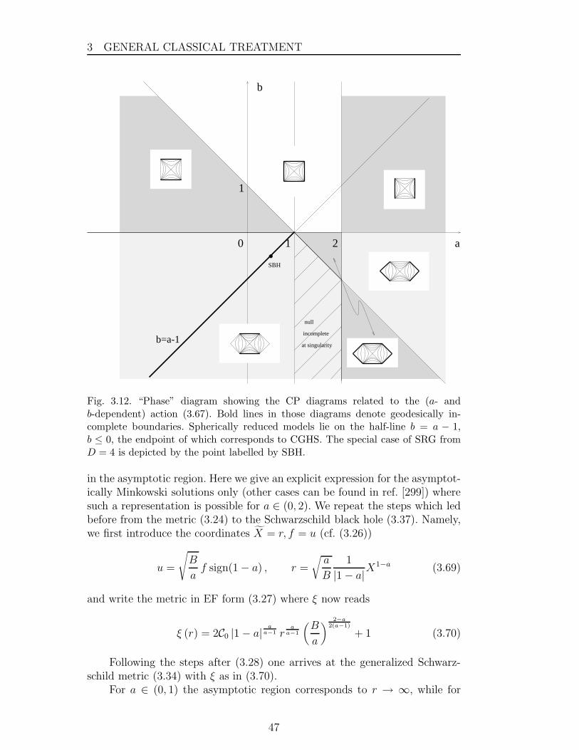
• Section 3 gives all classical solutions of GDTs in the absence of matter. Theglobal structure of such theories is discussed using Schwarzschild space-time as a simple example. As a further illustration we consider a family ofdilaton models describing a single black hole in Minkowski, Rindler or deSitter space-time.
• Section 4 extends the discussion to additional gauge-fields, supergravity and(bosonic or fermionic) matter fields.
• Section 5 considers the role of energy in GDTs. In particular, the ADMmass, quasilocal energy, an absolute conservation law and its correspondingNother symmetry are discussed.
• Section 6 leaves the classical realm providing a concise treatment of (semi-classical) Hawking radiation for minimally and non-minimally coupled mat-ter.
• Section 7 is devoted to non-perturbative path integral quantization of thegeometric sector of GDTs with (scalar) matter, giving rise to a non-localand non-polynomial effective action depending solely on the matter fieldsand external sources. The matter sector is treated perturbatively.
• Section 8 shows some consequences of the previously developed perturbationtheory: the virtual black hole phenomenon, the appearance of non-localvertices, and S-matrix elements for s-wave gravitational scattering.
• Section 9 describes the status of Dirac quantization for a typical exampleof that approach.
• Section 10 concludes with a brief summary and an outlook regarding openquestions.
• Appendix A recalls the spherical reduction procedure in the Cartan formal-ism.
• Appendix B collects some basic properties of the heat kernel expansionneeded in Section 6.
Several topics are closely related to the subject of this review, but are not
included:(1) Various calculations and explanations of the BH entropy [169, 355] be-
came a large and rather independent field of research which shows, how-ever, overlaps [165,171] with the general treatment of the dilaton theoriespresented in this review. We do not cover approaches which imply fur-ther physical assumptions which transgress the orthodox application ofquantum theory to gravity [34, 35, 43, 24, 31].
9
1 INTRODUCTION
(2) The ideas of the holographic principle [403,400] and of the AdS/CFT cor-respondence [309,200,444] are now being actively applied to BH physics(see, e.g. [375] and references therein).
(3) There exist different approaches to integrability of gravity models in twodimensions [338,269,268,339]. In particular, a rather sophisticated tech-nique has been applied to solve the effective 2D models emerging aftertoroidal reduction (instead of the spherical reduction considered in this re-view) of the four-dimensional Einstein equations [39,417]. Recently againinteresting developments should be noted in Liouville gravity [151, 406].Some relations between 2D dilaton gravity and the theory of solitonswere discussed in [70, 336].
Each of these topics deserves a separate review, and in some cases such reviewsexist. Therefore, we have restricted ourselves in those fields to just a few(somewhat randomly selected) references which hopefully will permit furtherorientation.
1.2 Differential geometry
1.2.1 Short primer for general dimensions
In the comprehensive approach advocated for D = 2 gravity the useof Cartan variables (zweibeine, spin-connection) plays a pivotal role. As anintroduction and in order to fix our notations we shall review briefly thisformalism. For details we refer to the mathematical literature (cf. e.g. [334]).
On a manifold with D dimensions in each point one introduces viel-beine eµa(x), where Greek indices refer to the (holonomic) coordinates xµ =(x0, x1, . . . , xD−1) and Latin indices denote the ones related to a (local) Lorentzframe with metric η = diag (1,−1, . . . ,−1). The dual vector space is spannedby the inverse vielbeine 12 eaµ(x):
eµaebµ = ηab (1.2)
SO(1, D− 1) matrices Lab(x) of the (local) Lorentz transformations obey
Lac Lbc = δab . (1.3)
A Lorentz vector V a = eaµVµ transforms under local Lorentz transformations
asV ′a(x) = Lab(x)V
b(x) (1.4)
This implies a covariant derivative
(Dµ)ab = δab ∂µ + ωµ
ab , (1.5)
12 For simplicity we shall use indiscriminately the term “vielbein” for the vielbein,the inverse vielbein and the dual basis of 1-forms (the components of which aregiven by the inverse vielbein) whenever the meaning is clear either from the contextor from the position of indices.
10
1 INTRODUCTION
if the spin-connection ωµab is introduced as the appropriate gauge field with
transformationω′µab = −Lbd (∂µL
ad) + Lac ωµ
cd Lb
d . (1.6)
The infinitesimal version of (1.6) follows from Lab = δab + lab + O(l2) wherelab = −lba .
Formally also diffeomorphisms
xµ(x) = xµ − ξµ(x) + O(ξ2) (1.7)
can be interpreted, at least locally, as gauge transformations, when the Lievariation is employed which implies a transformation referring to the samepoint. In
∂xµ
∂xν= δµν − ξµ, ν ,
∂xν
∂xµ= δνµ + ξν, µ (1.8)
partial derivatives with respect to xν have been abbreviated by the index aftera comma.
For instance, for the Lie variation of a tensor of first order Vµ(x) =∂xν
(1.15)where the sum is taken over all permutations π of 1, . . . , p + q and δπ is +1for an even number of transpositions and −1 for an odd number of transpo-sitions. It is convenient at this point to introduce the condensed notation for(anti)symmetrization:
α[µ1...µp] :=1
p!
∑
π
δπαaπ(1)...aπ(p), σ(µ1...µp) :=
1
p!
∑
π
σaπ(1)...aπ(p), (1.16)
where the sum is taken over all permutations π of 1, . . . , p and δπ is definedas before. In the volume form
Ωp=D =1
D!a[µ1...µD ] ǫ
µ1 ... µD dDx =1
D!a[µ1 ... µD] |e|ǫµ1 ... µDdDx (1.17)
the product of differentials must be proportional to the totally antisymmetricLevi-Civita symbol ǫ01...(D−1) = −1 or, alternatively, to the tensor ǫ = |e|−1ǫ(cf. (1.12)). The integral of the volume form
∫MD
ΩD on the manifold MD con-tains the scalar a = a[µ1 ... µD ] ǫ
µ1 ... µD which is the starting point to constructdiffeomorphism invariant Lagrangians.
can be defined which allows the introduction of the Hodge dual of Ωp as aD − p form
∗ Ωp = Ω′D−p =
1
p!(D − p)!ǫµ1 ... µD−p
ν1 ... νp Ων1 ... νpdxµ1 ∧ . . . ∧ dxµD−p .
(1.19)In D = even and for Lorentzian signature we obtain for a p-form
∗ ∗ Ωp = (−1)p+1Ωp. (1.20)
The exterior differential one form d = dxµ∂µ with d2 = 0 increases the formdegree by one:
dΩp =1
p!∂µΩµ1...µp
dxµ ∧ dxµ1 ∧ · · · ∧ dxµp (1.21)
Onto a product of forms d acts as
d (Ωp ∧ Ωq) = dΩp ∧ Ωq + (−1)pΩp ∧ dΩq . (1.22)
12
1 INTRODUCTION
We shall need little else from the form calculus [334] except the PoincareLemma which says that for a closed form, obeying dΩp = 0, in a certain(“star-shaped”) neighborhood of a point xµ on a manifold M, Ωp is exact, i.e.can be written as Ωp = dΩ′
p−1.In order to simplify our notation we shall drop the ∧ symbol whenever
the meaning is clear from the context.The Cartan variables expressed as one forms (1.13) in view of their
Lorentz-tensor properties are examples of algebra valued forms. This is alsothe case for the covariant derivative (1.5), now written as
Dab = δabd+ ωab , (1.23)
when it acts on a Lorentz vector.From (1.13) and (1.23) the two natural quantities to be defined on a
manifold are the torsion two-form
T a = Dab e
b (1.24)
(“First Cartan’s structure equation”) and the curvature two-form
Rab = Da
c ωcb (1.25)
(“Second Cartan’s structure equation”). From (1.23) immediately follows
(D2)ab = DacD
cb = Ra
b , (1.26)
Bianchi’s first identity. Using (1.26) D3 can be written in two equivalent ways,
DabR
bc −Ra
bDbc = 0, (1.27)
corresponding to Bianchi’s second identity
(dRab) + ωacRcb + ωbcR
ac =: (DR)ab = 0 . (1.28)
The l.h.s. defines the action of the covariant derivative (1.23) on Rab, a Lorentztensor with two indices. The brackets indicate that those derivatives only actupon the quantity R and not further to the right. The structure equationstogether with the Bianchi identities show that the covariant action for anygravity action in D dimensions depending on ea, ωab can be constructed as avolume form depending solely on Rab, T a and ea. The most prominent exampleis Einstein gravity in D = 4 [136, 135] which in the Palatini formulationreads [352]
LHEP ∝∫
M4
Rabeced ǫabcd , (1.29)
having used the definition ǫabcd = ǫµνστ eµaeνbeσc eτd. The condition of vanishing
torsion T a = 0 for this special case already follows from varying ωab indepen-dently in (1.29).
13
1 INTRODUCTION
In the usual textbook formulations of Einstein gravity, in terms of themetric, the affine connection Γµν
ρ appears as the only variable in the covariantderivative, e.g. for a contravariant vector Xν
Xν;µ := ∇µX
ν = (∇µ)νρX
ρ = (∂µδνρ + Γµρ
ν)Xρ. (1.30)
In the vielbein basis eaµ we relate Xb = ebρXρ and let (1.5) act onto that Xb.
Multiplying by the inverse vielbein (1.2) and comparing with (1.30) yields
Γµνρ = ea
ρ[(Dµ)
ab e
bν
]. (1.31)
The same identification follows, of course, from the covariant derivative of acovariant vector:
Xν;µ := ∂µXν − Γµνρ Xρ (1.32)
Covariant derivatives may be constructed easily also for tensors withmixed space-time and local Lorentz indices. For instance, that derivative act-ing upon the vielbeine eρc
(Dµ e)νa = [(Dµ)
νρ ]a
c eρc := (∇µ)νρ e
ρa + (ωµ)a
c eνc = 0 (1.33)
is seen to vanish. By (1.2) this implies the same result for analogously definedvielbeine eaρ
(Dµe)aρ = 0 . (1.34)
From (1.34) and the antisymmetry of ωab = −ωba (one version of metricity)corresponding to its property as a Lorentz generator of SO(1, D − 1) imme-diately
∇µgρσ = 0 (1.35)
can be derived, the version of the metricity usually employed in torsionlesstheories.
Comparing the antisymmetrized part of the affine connection Γ[µν]ρ =
12(Γµν
ρ − Γνµρ) of (1.31) with the components of the torsion (1.24), multiplied
by the inverse vielbein, shows that the expressions are identical:
eρa Taµν = Γ[µν]
ρ . (1.36)
This allows to express the full affine connection
Γµνρ = Γ(µν)
ρ + Tµνρ (1.37)
in terms of Christoffel symbols µ, ν, ρ and the contorsion K
Γ(µν)ρ = gρσ Γ(µν)σ = µ, ν, ρ + K(µν)ρ (1.38)
by the standard trick of considering (1.35) in the form
gνρ,µ = Γµνλ gλρ + Γµρ
λ gλν (1.39)
14
1 INTRODUCTION
with (1.38) and by taking the linear combination of the identity (1.39) minusthe one for gµν,ρ plus the one for gρµ,ν . In this way the Christoffel symbol
µ, ν, ρ =1
2(gνρ,µ + gµρ,ν − gµν,ρ) , (1.40)
but also the additional contorsion contribution K from the nonvanishing tor-sion in (1.38)
K(µν)ρ = T[ρµ]ν + T[ρν]µ (1.41)
can be found. Nonvanishing torsion and thus also a nonvanishing contorsionare important for the determination of the global properties of a certain solu-tion of a generic theory of gravity.
In contrast to ordinary Minkowski space field theories, the variables ofgravity – in the most general case the independent Cartan variables e andω – in the dynamical evolution also determine the non-Minkowski dynamicalbackground upon which the theory lives. Thus, for the investigation of thatbackground a device must be found which acts like a test charge in an elec-tromagnetic field. The simplest possibility in gravity is to add the Lagrangianof a point particle with path xµ = xµ(τ) to the original action ( ˙xµ = dxµ/dτwith the affine parameter τ),
L(p) = −mτ2∫
τ1
ds = −mτ2∫
τ1
√gµν(x) ˙xµ ˙xν dτ , (1.42)
with a mass m, small enough to be of negligible gravitational influence. Vari-ation of L(p) with respect to xµ leads to the usual geodesic equation
¨xµ + Γ(ρσ)µ ˙xρ ˙xσ = 0 , (1.43)
where, by construction from (1.42), Γ(ρσ)µ = gµα ρ, σ, α only “feels” the
Christoffel part (1.40) of the affine connection and not the contorsion (1.41).Alternatively, also the full affine connection Γ may be considered in (1.43)(“autoparallels”) [217,218]. For that modified geodesic equation for xα(τ) alsoa (non-local) action replacing (1.42) can be found in the literature [160, 262].In order to explore the local and topological properties of a certain manifoldwhich corresponds to a solution of a generic gravity theory all points mustbe connected which can be reached by a device like the geodesic (1.43) bymeans of a time-like, but also space-like or light-like path. The classificationof possible extensions of a certain patch uses the notion of “geodesic” incom-pleteness: a geodesic which has only a finite range of affine parameter, butwhich is inextendible 13 in at least one direction is called incomplete. A space-time with at least one incomplete (time/space/light-like) geodesic is called(time/space/light-like) geodesically incomplete. The notion of incompleteness
13 This means the corresponding geodesic must have (at least) one endpoint. Fordetails we refer to [216,428].
15
1 INTRODUCTION
also yields the most satisfactory classification of (geometric) singularities. Forexample, a singularity like the one in the Schwarzschild metric [386] can bereached by at least one (time- or light-like) geodesic with finite affine param-eter (i.e. with finite proper time for massive test particles).
For D = 2 theories a complete discussion of “geodesic topology” forany generic theory can be carried out (cf. sect. 3.2.) [430, 264]. Here we justwant to emphasize the importance of the type of device to be used for thedetermination of the “effective” topology of the manifold which, in principle,may be different for geodesics, autoparallels, spinning particles etc. .
1.2.2 Two dimensions
In D = 2 the Lorentz transformations (1.3),(1.4) simply reduce to a boostwith velocity v
Lab =
cosh v sinh v
sinh v cosh v
a
b
= δab + ǫab v + O(v2) , (1.44)
where in local Lorentz indices with metric ηab = ηab (η = diag(+1,−1)) theLevi-Civita symbol ǫab = ηac ǫcb (ǫ01 = −ǫ01 = +1) coincides with the tensor.It is related to the tensor ǫµν in holonomic coordinates (cf. (1.17)) by (explicitvalues of Lorentz indices in (1.47) are underlined)
ǫ = −1
2ǫabe
a ∧ eb (1.45)
ǫµν = eaµebνǫab = |e|ǫµν = |e|−1gµρgνσ ǫ
ρσ , (1.46)
|e| = det eaµ = e00 e
11 − e
10 e
01 . (1.47)
It should be noted that in (1.45) we choose the sign, which differs from (1.14),in order to be consistent with some original literature. As there is only onegenerator εab in SO(1, 1) (cf. (1.44)) the spin connection one-form simplifiesto a single term ωab = ω ǫab and hence the one quadratic in ω of Rab (1.25)vanishes:
Rab = ǫab dω . (1.48)
From now on for simplicity we shall refer to the 1-form ω as the “spin connec-tion”.
This shows that the curvature in D = 2 only possesses one independentcomponent which we take to be the Ricci-scalar 14 :
R = 2 ∗ dω = 2|e|−1ǫρσ∂ρωσ . (1.49)
14 Our convention corresponds to the contraction Rµννµ = Rµν abe
aνebν where Rµν abare the tensor components of Rab. Rµν
ρσ then coincides with the usual textbookdefinition [428].
16
1 INTRODUCTION
It is clear from this expression that the Hilbert-Einstein action in two di-mensions is a total divergence. In (compact) Euclidean space (
√−g → √g)
without boundaries it becomes the Euler characteristic of a 2D Riemannianspace with genus γ ∫
Mγ
d2x√g R = 8π(1 − γ) . (1.50)
Also the torsion simplifies to a volume form
T a =1
2Tµν
adxµ ∧ dxν , Tµνa = (Dµeν)
a − (Dνeµ)a , (1.51)
with(Dµ)
ab = ∂µδ
ab + ωµǫ
ab . (1.52)
The Hodge dual of T a here is a diffeomorphism scalar:
τa := ∗ T a = |e|−1 ǫµν (Dµeaν) (1.53)
In D = 2 the inverse of the zweibeine from (1.2) obeys the simple relation
eµa = −|e|−1ǫµν ǫab ebν . (1.54)
The formula for the change of the Ricci scalar under a conformal trans-formation of the metric gµν = e2ρ gµν is most easily derived from a transfor-mation eaµ = eρ eaµ of the zweibeine for vanishing torsion T a = 0, i.e. withω = ω = ea ∗ dea in the Ricci scalar (1.49)
|e|R = 2|e| ∗ d(ea ∗ dea) = 2 ǫτσ∂τ
(eσa ǫµν
|e| ∂µeaν). (1.55)
Remembering e = |e|e2ρ and using (1.54) for eµaeνbη
ab = gµν yields ((e) =√−g)
an important identity:√−g R =
√−gR− 2∂τ (√−ggτσ ∂σρ) . (1.56)
Light-cone Lorentz vectors are especially useful in D = 2,
X± :=1√2
(X0 ±X1) , (1.57)
yielding X2 = XaXa = X aXa = ηabXaX b = 2X+X− with metric
ηab =
0 1
1 0
(1.58)
and the corresponding Lorentz ǫ-tensor ǫab = ηa c ǫc b with ε±± = ±1. The lightcone components of the torsion (1.51) become
T± = (d± ω) e±. (1.59)
17
1 INTRODUCTION
Since we are going to discuss fermionic matter (as well as supergravity)we have to fix our spinor notation. The γa-matrices are defined in a localLorentz frame
γa, γb
= 2ηab (1.60)
γ0 =
0 1
1 0
, γ1 =
0 1
−1 0
γ∗ := −γ0γ1 =
1 0
0 −1
= −1
2
[γ0, γ1
].
(1.61)
In light cone components we obtain a representation in terms of nilpotentmatrices
γ+ =√
2
0 1
0 0
, γ− =
√2
0 0
1 0
(1.62)
The covariant derivative acting on two-dimensional Dirac fermions
Dµ = ∂µ −1
2γ∗ ωµ (1.63)
is determined by the Lorentz generator for spinors [γ0, γ1]/4 = −γ∗/2.
18
2 MODELS IN 1 + 1 DIMENSIONS
2 Models in 1 + 1 Dimensions
There are (at least) four different motivations to study generalized dilatontheories (GDT) in D = 2:• Starting from Einstein gravity in D ≥ 4 and imposing spherical symmetry
one reproduces a certain GDT• A certain limit of (super-)string theory yields a particular GDT as effective
action• GDTs can be viewed as toy models for quantization of gravity and as a
laboratory for studying BH evaporation• In a first order formulation the underlying Poisson structure reveals relations
to non-commutative geometry and deformation quantization. Again, GDTsare a convenient laboratory to elucidate these new concepts and techniques.
Moreover, a result obtained along one route is of course also valid for all otherapproaches after having translated the jargon from one field to the others. Inthis sense, GDTs may even serve as a link between general relativity (GR),string theory, BH physics and non-commutative geometry.
We base our discussion on the first (somewhat more phenomenological)route and show the links to the other fields in this section.
2.1 Generalized Dilaton Theories
2.1.1 Spherically reduced gravity
The introduction of dilaton fields allows the treatment of the dynamicsfor a generic higher dimensional (D > 2) theory of gravity in an effectivetheory at lower dimension D1 < D, which is still diffeomorphism invariant. Incertain special cases the isometry group of the D-dimensional metric is suchthat it allows for a reduction to D1 = 2. Important examples for D = 4 aretoroidal reduction [273, 189, 178, 225, 56] and spherical reduction [36, 412, 33,409,205,324,407,244,276,295,195]. The latter is of special importance, becauseit covers the Schwarzschild BH. Therefore, we concentrate on that example.
Splitting locally the D-dimensional manifold MD into a direct productM2 × SD−2 the line element becomes
(ds)2(D) = gµν(x)dx
µdxν − λ−2X2
D−2 (dΩ)2SD−2 (2.1)
where (dΩ)2SD−2 is the surface element of the (D−2)-dimensional sphere, xµ =
x0, x1 are the coordinates in M2, and λ is a parameter of mass dimensionone. A straightforward calculation (cf. e.g. [197]; explicit formulae for thecurvature 2-form, the ensuing Ricci-scalar and the Euler- and Pontryagin-classcan be found in appendix A) for the D-dimensional Hilbert-Einstein action
19
2 MODELS IN 1 + 1 DIMENSIONS
LHE =∫dDx
√−g(D)R(D) yields ((∇X)2 = gµν∂µX∂νX)
L(SRG) =OD−2
λD−216πGN
∫d2x
√−g[XR+
D − 3
D − 2
(∇X)2
X− λ2(D − 2)(D − 3)X
D−4D−2
]. (2.2)
In the prefactor, which will be dropped consistently in the following, OD−2
denotes the surface of the unit sphere SD−2. Fixing the 2D diffeomorphisms(partially) as X = (λr)D−2 (the radius r representing one of the coordinatesand λ > 0) eq. (2.1) yields the usual spherically symmetric line element inwhich r > 0 is required.
Another way to obtain a 2D theory from a higher dimensional one is tosuppose that the D-dimensional manifold is a direct product MD = M2 ⊗TD−2, where TD−2 is a torus, and that all fields are independent of the D −2 extra coordinates. This procedure is called dimensional reduction. It alsoproduces a dilaton theory in 2D if the higher dimensional theory alreadycontains the dilaton [180].
2.1.2 Dilaton gravity from strings
Developments in string theory contributed much to the increase of interestin dilaton gravity in the 1990s. The simplest way to obtain it from strings isto consider the conditions for world-sheet conformal invariance [72].
The starting point is the non-linear sigma model action for the closedbosonic string,
L(σ) =1
4πα′
∫d2ξ
√−h
[gµνh
ij∂iXµ∂jX
ν + α′ΦR], (2.3)
where ξ is a coordinate on the string world-sheet, hij is a metric 15 there, Rrepresents the corresponding scalar curvature. The other symbols denote: thetarget space coordinates (Xµ), the target space metric (gµν), and the dilatonfield (Φ). As usual, α′ is the inverse string tension. The antisymmetric B-fieldis set to zero.
It is essential for string consistency that, as a quantum field theory, thesigma model be locally scale invariant. This is equivalent to the requirementthat the trace of the 2D world-sheet energy-momentum tensor vanishes. Itsgeneral structure is
2πT ii = βΦR + βgµνhij∂iX
µ∂jXν , (2.4)
where the “beta functions” βΦ and βgµν are local functionals of the couplingsgµν and Φ, usually calculated in the form of a power series in α′. Note that thefirst term in L(σ) is conformally invariant and contributes to the β-functions
15 This metric should not be confused with gµν restricted to D = 2 in (2.8).
20
2 MODELS IN 1 + 1 DIMENSIONS
at the quantum level only through the conformal anomaly. It corresponds toO(α′)0. The second term in (2.3) breaks local scale invariance already at theclassical level. Due to the factor α′ its contributions to the trace (2.4) also startwith the zeroth power of α′. The leading terms in βΦ and βgµν were calculatedin ref. [72]. With our sign conventions they read:
βΦ
α′ = − λ2
4π2− 1
16π2
(4(∇Φ)2 − 4∇µ∇µΦ − R
), (2.5)
βgµν = Rµν + 2∇µ∇νΦ , (2.6)
where ∇µ is the covariant derivative in target space, R is the scalar curvatureof the target space manifold. The constant λ depends on the central charge.For the bosonic string it is
λ2 =26 −D
12α′ . (2.7)
This constant vanishes for critical strings.The key observation regarding the beta functions (2.5) and (2.6) is that
the conditions of conformal invariance βΦ = 0 and βgµν = 0 are equivalent tothe e.o.m.-s to be derived from the dilaton gravity action
L(dil) =∫dDX
√−ge−2Φ[R + 4(∇Φ)2 − 4λ2
]. (2.8)
In particular, the dilaton e.o.m. is equivalent to βΦ = 0. The Einstein equationsare given by a combination of the two beta functions, βgµν − 8π2gµνβ
Φ/α′ = 0.For D = 2 the action (2.8) describes the geometric part of the “string
inspired” dilaton (CGHS) model [71] which has been studied since the early1990-s [326,77,32,330,277,416]. It is intimately related to the SO(2, 1)/U(1)-WZW exact conformal field theory 16 [310, 137, 443,127].
An amusing feature of (2.8) with D = 2 is that after the identificationX = e−2Φ it can be obtained from (2.2) by taking there the limit D → ∞keeping λ2(D − 2)(D − 3) → const. = 4λ2 . This corresponds to the classicallimit α′ → ∞.
2.1.3 Generalized dilaton theories – the action
A result like (2.2) or (2.8) suggests the consideration of GDTs
L(dil) =∫d2x
√−g[R
2X − U(X)
2(∇X)2 + V (X)
], (2.9)
where the overall factor has been chosen for later convenience. Clearly aneven more general action could contain still another arbitrary function Z(X),replacing X in the first term of the square bracket [19, 349]. However, we
16 The non-compact form is SO(2, 1)/SO(1, 1). An early review on 2D gravity and2D string theory from the stringy point of view is ref. [186].
21
2 MODELS IN 1 + 1 DIMENSIONS
assume that Z(X) is invertible for the range of X to be considered 17 . Thisallows the inversion X = Z−1 (X) and the reduction to the form (2.9). Indeedthe “physical” applications seem to be always of that type. The BH singularityof SRG reveals itself in the singular factor U of the dynamical term for thedilaton field. This is the first hint to the fact that the “strength” of thatsingularity in the solution of (2.2) is not fixed by the action; it will actuallyturn out to be a “constant of motion” which for the BH coincides with theADM mass (cf. sect. 5).
An alternative representation is suggested by (2.8):
L(dil) =1
2
∫d2x
√−ge−2Φ[R− U(Φ)(∇Φ)2 + 2V (Φ)
], (2.10)
with U(Φ) = 4 exp (−2Φ)U(exp (−2Φ)) and V (Φ) = exp (2Φ)V (exp (−2Φ)).Eqs. (2.9) and (2.10) are related by the redefinition of the dilaton field
X = e−2Φ, (2.11)
explicitly taking into account positivity ofX which is required in many models.Among the GDTs (2.9) with U(X) = 0 the simplest nontrivial choice of
refs. [22, 123, 405,122,124,239]
VJT = ΛX, UJT = 0 , (2.12)
the Jackiw-Teitelboim (JT) model, has played a decisive role for the under-standing of 2D (lineal) gravity [238]. Depending on the sign of Λ it describesa 2D (anti-) de Sitter manifold with constant positive or negative curvature.The symmetry properties of the model are related to the Lie algebra SO(1, 2).It has been explored in detail in the quoted references. Below this algebra willturn out to represent the special linear case of some, in general, nonlinear (fi-nite W -) algebra [118] associated with a generic dilaton theory (2.9) (cf. Sect.2.3).
More complicated models with U(X) = 0, but V (X) exhibiting a singu-larity in X, among others may also involve solutions with space-time structureof a BH or its generalizations. E.g. the choice 18
VRN = −2M
X2+
Q2
4X3(2.13)
produces a line element like the one for the Reissner-Nordstrom BH withcharge Q and mass M [364, 346]. Evidently in this case the singularities are
17 To the best of our knowledge there is no literature on nontrivial models whereZ(X) is not invertible (cf. also [397]). By a suitable redefinition a different simpli-fication with U(X) = 1, Z(X) 6= 1 was proposed in ref. [373].18 Solving the general theory in Sect. 3.1 we shall find that the potentials U andV as in (2.9) determining a dilaton action can even be ‘designed’, starting from agiven line-element.
22
2 MODELS IN 1 + 1 DIMENSIONS
kept fixed by parameters of the action. They cannot be related to the conser-vation law referred to already above for a “dynamical” model with singularnonvanishing U(X) and regular V (X). A final remark for the case U = 0 con-cerns the possibility to eliminate the dilaton field altogether by means of thealgebraic equations of motion produced by varyingX in (2.9), V ′ (X) = −R/2.If this equation can be inverted, the dilaton Lagrangian for U = 0 turns intoa Lagrangian depending on the function of R alone [380, 168,381,397]:
L =∫d2x
√−g f(R) (2.14)
As compared to such theories (2.14), the literature on models generalized soas to depend also on torsion (cf. (1.53))
L =∫d2x
√−g h (R, τaτa) (2.15)
is relatively scarce. It mainly consists of elaborations based upon the model ofKatanaev and Volovich [250, 251] where the function h in (2.15) is quadraticin R and linear in τaτa, also known as “Poincare gauge gravity” [390,389,391,392,348,322].
Models with U(X) 6= 0 and different assumptions for that function andV (X) have been studied extensively (cf. e.g. [312,19,349,350,374,373,41,116,311, 173, 304, 303, 298]). For their solution throughout these works the con-formal or the Schwarzschild gauge have been used, leading to complicatede.o.m.-s, the solution of which often requires considerable mathematical ef-fort. Because we shall avoid this complication altogether (sect. 3) no explicitexamples of this approach will be given here.
2.1.4 Conformally related theories
Sometimes, it is convenient [306, 337, 255, 114, 293, 88, 112, 84, 89] to usea conformal transformation (1.56) with ρ(X) = −1/2
∫X U(y) dy in (2.9) tosimplify the dynamics by the transition to a new theory with U = 0 andV (X) = V (X) exp(−2ρ). One has to keep in mind, however, that the twotheories need not be equivalent physically. To interpret the results one mustalways return to the original theory. This subtlety was sometimes ignored. Onesource of this misunderstanding seems to be that in field theory the transfor-mation of field variables in a fixed flat Minkowski background is allowed, aslong as such a transformation is regular. For a GDT (2.9) with singular Uthis has to fail for two reasons. The first one is that such a conformal trans-formation must be singular in order to compensate for a singularity in U(X).Still one could argue that locally such a transformation should be permissible.However, and this is the second crucial reason, in gravity the field theory in itsvariables at the same time determines the (dynamical!) manifold upon whichit lives. For a singular conformal transformation the new manifold can possesscompletely different topological properties.
23
2 MODELS IN 1 + 1 DIMENSIONS
An extreme example is the CGHS model (2.8) [71] which from a Schwarz-schild-like topology may be transformed into flat (Minkowski) space. The rea-son can be seen most easily in the transformation behavior of geodesics: onlynull geodesics are mapped onto (in general non-affinely parameterized) nullgeodesics and their corresponding affine parameters are related by [428]:
dτ
dτ∝ e2ρ (2.16)
If ρ approaches infinity at a certain point, by such a singular conformaltransformation geometric properties like geodesic (in)completeness can be al-tered 19 .
In fact, this misunderstanding had been clarified already half a centuryago [153] in connection with the Jordan-Brans-Dicke theory in D = 4 [240,241, 51]. There already in D = 4 a “Jordan-field” X in a D = 4 action like(2.9) with U(X) = const. is introduced. The D = 4 version of identity (1.56),together with an appropriate transformation of X may be used to transformthat action so that the term involving R is reduced to the Hilbert-Einsteinform. At that time a controversy arose whether the latter (the “Einstein-frame”) or the original one (the “Jordan frame”) was the “correct” one. Asargued by Fierz [153] the answer to that questions depends on the definition ofgeodesics, to be used for the determination of the global topology (cf. sect. 1.2).A geodesic depending on the metric g in the Jordan frame is quite differentfrom the one which feels the metric of the conformally transformed g in theEinstein-frame. Of course, for a (globally) regular conformal transformationΩ2, gµν = Ω2 gµν it would be perfectly correct to simultaneously transform ginto the Jordan frame. But then the equation of the geodesic, when expressedin terms of g acquires an additional dependence on Ω(X), i.e. the test particlewould feel a non-geodesic external force exerted by the Jordan-field X.
The confusion in D = 2 probably also originated from the by now veryfamiliar situation in string theory [191,360]. Its conformal invariance does notcarry over automatically to the world-sheet, where it is achieved by imposingthe e.o.m.’s in target space (cf. sect. 2.1.2). String theory yields dilaton gravityas its low energy limit also in higher dimensions. In that context the Jordanframe usually now is called the string frame and the old discussion referred toin the previous paragraph has been resurrected in modern language [78, 126,83, 152, 5].
A simple example of a singular conformal transformation leading to achange of (timelike) geodesic (in)completeness can be found in fig. 9.1 of [428].Another obvious case is provided by the Schwarzschild metric, eq. (3.37) be-low. A (singular) conformal transformation with Ω2 = ξ−1 = (1 − 2M/r)−1
19 Since the usual conformal transformation involved in this context is proportionalto the integral of U(X) and the latter has a singularity in practically all physicallyinteresting models there will be at least one such singular point in addition to the(asymptotic) singularity at X → ∞ [193].
24
2 MODELS IN 1 + 1 DIMENSIONS
and a (singular) coordinate transformation r =∫ r dy/ξ(y) leads to Minkowski
spacetime. This is, of course, a rather trivial consequence of (patchwise) con-formal flatness of any 2D metric. It will be discussed below why ADM mass(sect. 5.1) and Hawking radiation (sect. 6) are, in general, different in confor-mally related theories.
2.2 Equivalence to first-order formalism
Cartan variables have been introduced in sect. 1.2 in order to formulate avery general class of D = 2 first order gravity (FOG) theories by the covariantHamiltonian action
L(FOG) =∫
M2
[Xa(De)a +Xdω + ǫV(XaXa, X)] , (2.17)
which seems to have been introduced first for the special case (V = 0) instring theory [426], then considered for a special model in ref. [230] and finallygeneralized to the in D = 2 most general form (2.17) for a theory of puregravity in refs. [396, 379]. It depends on auxiliary fields Xa and X so that itis sufficient to include only the first derivatives of the zweibeine (torsion) andof the spin connection (curvature). The whole dynamical content is encodedin a (Lorentz-invariant) potential V multiplied by the volume form (1.45). Inthe following very often light-cone coordinates (1.57) and (1.59) will be used:
Xa(De)a = X+(d− ω) e− +X−(d+ ω) e+ (2.18)
We also recall (1.49), the relation 2 ∗ dω = R between spin-connection andcurvature scalar.
The component version of (2.17) with (1.49) follows from the identifica-tion (cf. (1.53),(1.55)) implying the Hodge-duals,
(d± ω)e± ⇒ ǫµνd2x1
2T±µν = (e) τ±d2x ,
dω ⇒ ǫµν∂µωνd2x = (e)
R
2d2x ,
ǫ⇒ −1
2ǫabe
aµebν ǫµνd2x = (e) d2x ,
(2.19)
as
L(FOG) =∫d2x
ǫµν [X+(∂µ − ωµ)e
−ν +X−(∂µ + ωµ)e
+ν
+X ∂µων ] + (e)V(2X+X−, X). (2.20)
The original intention of the formulation (2.17) had been to express ageneral 2D Lagrangian involving the only independent geometric quantities
25
2 MODELS IN 1 + 1 DIMENSIONS
(Ricci scalar R, and torsion scalar T 2 = τaτa = 2τ+τ−, cf. (1.53),(2.15))
L(R,τ2) =∫d2x
√−g h(R, τ 2) (2.21)
in a simpler fashion. The variables Xa and X can be eliminated by the alge-braic e.o.m.-s from variation δXa, δX in (2.17) or (2.20),
τa +∂V∂Xa
= 0 ,R
2+∂V∂X
= 0 , (2.22)
provided the Hessian | ∂2V/∂XA∂XB | does not vanish (XA = X,Xa). Evi-dently this is not always possible, but also, inversely, not every action L(R, τ 2)permits a reformulation as L(FOG) in (2.17) 20 .
Fortunately the relation of (2.17) to GDT (2.9) and especially to modelswith a physical motivation (e.g. SRG) is more immediate and subjected toweaker conditions. Then, instead, only Xa and the torsion-dependent part ofthe spin connection are eliminated by e.o.m.-s which are linear and algebraicand thus may be reinserted into the action 21 . From the definition for ∗T a(1.53) with ω = ωaea in the local Lorentz basis ea, the identities ea∧eb = −ǫab·ǫand ∗ ǫ = 1, one gets
∗T a = ∗ dea − ωa (2.23)
orω = ωaea = ea ∗ dea − ea ∗ T a =: ω − ∗T , (2.24)
where ω represents the torsion free part of the spin connection.The e.o.m. from variation of Xa in (2.17)
dea + ǫab ω ∧ eb + ǫ∂V∂Xa
= 0 , (2.25)
after taking the Hodge dual, multiplication with ea and comparison with theidentity (2.24) yields the relation between ∗T and V
∗T = −ea∂V∂Xa
. (2.26)
Reinserting this algebraic eq. into (2.17) produces
L(FOG)1 =
∫
M2
[Xaǫab
∂V∂ Xc
ec ∧ eb +Xdω − dX ∧ ec ∂V∂Xc
+ ǫV], (2.27)
where the torsion dependent part of ω now has been eliminated, but thedependence on Xa is retained. For potentials ∂V/∂Xa = 0 eq. (2.27) already
20 For a mathematically more precise discussion of this point we refer to ref. [397].21 This equivalence has been published first in ref. [248] for the KV-model [250,251].The proof below follows the formulation used in ref. [141] for the even more generalcase of 2D dilaton supergravity (cf. also sect. 4.2).
26
2 MODELS IN 1 + 1 DIMENSIONS
by the second and third eq. (2.19) can be identified directly as GDT (2.9) withU = 0,V(X) = V (X). When ∂V/∂Xa 6= 0 the e.o.m. from δXa in (2.27) mustbe used,
(dX ∧ ec +Xcǫ)∂2V
∂Xc ∂Xa= 0 , (2.28)
which for nonvanishing Hessian of V, now with respect to the Xa alone, leadsto 22
Xa = ∗ (ea ∧ dX) =ǫµν
(e)eaµ (∂νX) . (2.29)
For easy comparison with the GDT (2.9), before using (2.29) and (2.27),the latter action is rewritten in component form. After cancellation of twoterms with ∂V/∂Xa the final result is very simple
L(dil) =∫d2x (e)
[XR
2+ V(−(∇X)2, X)
], (2.30)
where, according to (2.29), the argument XaXa in V has been replaced by asecond derivative term of X, to be identified also here with the same dilatonfield as in (2.9). The curvature scalar R = ∗2dω refers to the torsionless partof the spin connection in (2.24). Thus it may be expressed equally well directlyby the 2D metric gµν .
For potentials quadratic in the torsion-related variable Xa
V = U(X)XaXa
2+ V (X) (2.31)
the action (2.30) exactly coincides with (2.9) in which torsion had been zerofrom the beginning. As we have used the algebraic (and even only linear)e.o.m.-s to reduce the configuration space of L(FOG) to the one of L(dil), the twoactions lead to the same dynamics. This equivalence can be verified easily aswell by the study of the explicit analytic solution (cf. sect. 3.1). We anticipatealso that at the quantum level the steps above can be simply reinterpreted as“integrating out” the torsion dependent part of ω and Xa [281], cf. footnote61 on page 85.
Apart from covering torsionless dilaton theories (2.9), the first order for-mulation (2.17) also permits the inclusion of 2D theories with nonvanishingtorsion. The choice
VKV =α
2XaXa +
β
2X2 − Λ , (2.32)
after elimination of Xa and X according to (2.22) produces the KV model[250, 251] which is quadratic in curvature and torsion and thus of the type of“Poincare gauge” theory [217, 218]. By our equivalence relation it could alsohave been written as the corresponding dilaton theory (2.9), of course.
22 For potentials V of the form (2.31) eq. (2.29) does not hold necessarily at pointsX0 where U(X0) = 0.
27
2 MODELS IN 1 + 1 DIMENSIONS
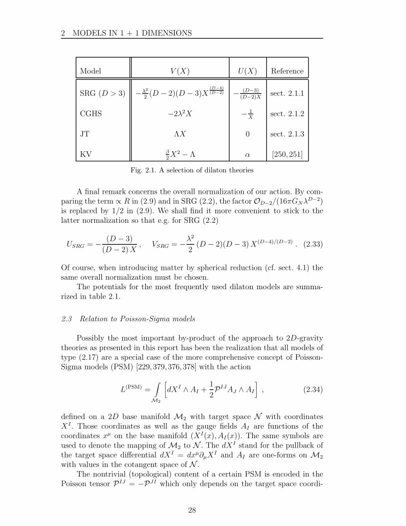
Model V (X) U(X) Reference
SRG (D > 3) −λ2
2(D − 2)(D − 3)X
(D−4)(D−2) − (D−3)
(D−2)Xsect. 2.1.1
CGHS −2λ2X − 1X
sect. 2.1.2
JT ΛX 0 sect. 2.1.3
KV β2X2 − Λ α [250, 251]
Fig. 2.1. A selection of dilaton theories
A final remark concerns the overall normalization of our action. By com-paring the term ∝ R in (2.9) and in SRG (2.2), the factor OD−2/(16πGNλ
D−2)is replaced by 1/2 in (2.9). We shall find it more convenient to stick to thelatter normalization so that e.g. for SRG (2.2)
USRG = − (D − 3)
(D − 2)X, VSRG = −λ
2
2(D − 2)(D − 3)X(D−4)/(D−2) . (2.33)
Of course, when introducing matter by spherical reduction (cf. sect. 4.1) thesame overall normalization must be chosen.
The potentials for the most frequently used dilaton models are summa-rized in table 2.1.
2.3 Relation to Poisson-Sigma models
Possibly the most important by-product of the approach to 2D-gravitytheories as presented in this report has been the realization that all models oftype (2.17) are a special case of the more comprehensive concept of Poisson-Sigma models (PSM) [229,379,376,378] with the action
L(PSM) =∫
M2
[dXI ∧AI +
1
2PIJAJ ∧ AI
], (2.34)
defined on a 2D base manifold M2 with target space N with coordinatesXI . Those coordinates as well as the gauge fields AI are functions of thecoordinates xµ on the base manifold (XI(x), AI(x)). The same symbols areused to denote the mapping of M2 to N . The dXI stand for the pullback ofthe target space differential dXI = dxµ∂µX
I and AI are one-forms on M2
with values in the cotangent space of N .The nontrivial (topological) content of a certain PSM is encoded in the
Poisson tensor PIJ = −PJI which only depends on the target space coordi-
28
2 MODELS IN 1 + 1 DIMENSIONS
nates. This tensor may be related to the Schouten-Nijenhuis bracket [383,340]
XI , XJ = PIJ (2.35)
which is assumed to obey a vanishing bracket of P with itself, i.e. nothingelse than a Jacobi identity which expresses the vanishing of the Nijenhuistensor [340]
PIL ∂PJK
∂XL+ cycl (I, J,K) = 0 . (2.36)
Only for PIJ linear in XI (in gravity theories the Jackiw-Teitelboim model[22, 123, 405, 122, 124, 238]), eq. (2.36) reduces to the Jacobi identity for thestructure constants of a Lie algebra and becomes independent of X. In generalthe algebra (2.35) with (2.36) covers a class of finite W-algebras [118]. Earlyversions of this nonlinear algebras from 2D gravity were discussed as constraintalgebra of the Hamiltonian in the context of the KV-model in [192], and withscalar and fermionic matter in [278]. The interpretation as a nonlinear gaugetheory in a related approach goes back to [230, 229].
Although we are dealing with bosonic fields in the present section ournotation anticipates already the graded PSM (gPSM) of supergravity in sect.4.3. Thus the index summation in (2.34) is in agreement with the conventionused in supersymmetry and (just here and in sect. 4.3) we shall also defineinstead of (1.22) the exterior differentiation to act from the right:
d(Ωp ∧ Ωq) = Ωp ∧ dΩq + (−1)qdΩp ∧ Ωq (2.37)
In the bosonic PSM for 2D gravity the action (2.34) reduces to (2.17) withthe identification
XI → (X,Xa) , AI → (ω, ea) . (2.38)
The component PaX of PIJ is determined by local Lorentz transformation forwhich (cf. (2.43) below)
PaX = Xbǫba (2.39)
is the generator. The components
Pab = V ǫab (2.40)
contain the potential V(Y,X) which determines the specific model (Y =XaXa/2).
With the present convention (2.37), the e.o.m.-s from (2.34) become
dXI + PIJAJ = 0 (2.41)
dAI +1
2
(∂PJK
∂XI
)AK ∧AJ = 0 . (2.42)
The identities (2.36) are the essential ingredient to show the validity of the
29
2 MODELS IN 1 + 1 DIMENSIONS
symmetries 23
δXI = PIJ ǫJ , (2.43)
δAI = −d ǫI −(∂PJK
∂XI
)ǫK AJ (2.44)
in terms of the local infinitesimal parameters ǫI(x). Eq. (2.44) reveals the gaugefield property of AI . Whereas for 2D gravity with (2.38), (2.39), (2.40) localLorentz-transformations (ǫI → ǫX) can be extracted easily from (2.43) and(2.44), diffeomorphisms (1.9) are obtained by considering ǫI = ξµAµI [396].Evidently (2.34) is invariant under target space diffeomorphisms too. Onlywhen those transformations are diffeomorphisms also globally, the topology ofM2 remains unchanged. It should be noted that conformal transformationsof the world sheet metric can be expressed as target space diffeomorphisms.Otherwise the problems discussed in sect. 2.1.4 are relevant also at the present,more general, level. Singular target space reparametrization (analogous to theconformal transformations discussed there) could eliminate singularities of themanifold M2 if the identification (2.38) of the PSM variables is retained.Of course, an appropriate simultaneous (singular) redefinition in the relationbetween AI and the Cartan variables could formally keep the topology ofM2 in terms of the new variables intact, at the price of those singularitiesappearing in the relation between AI and (ea, ω).
In 2D gravity the Poisson tensor PIJ is not of full rank, because thenumber of target space coordinates is odd. This also may happen for generalPSM-s and it implies the existence of “Casimir functions”, whose commutatorwith XI in the sense of (2.35) vanishes. In 2D gravity there is only one suchfunction 24
XI , C = PIJ ∂C∂XJ
= 0 . (2.45)
The conservation of C with respect to both coordinates of the manifold
dC = dXI ∂C∂XI
= −PIJ AJ∂C∂XI
= 0 (2.46)
follows from (2.45) and the use of (2.41) in (2.46). Lorentz-invariance requiresC = C(Y,X) with Y = XaXa/2 and thus according to (2.45) C must obey (cf.(2.39) and (2.40))
∂C∂X
− V(Y,X)∂C∂Y
= 0 . (2.47)
23 Applying (2.43) and (2.44) to the commutator of infinitesimal transformationsthe resulting one is again a symmetry only if the e.o.m.-s (2.41) are used, or if PIJ
is linear in X [397].24 For more details regarding generic PSM-s with more Casimir functions C we referto ref. [397].
30
2 MODELS IN 1 + 1 DIMENSIONS
This partial differential equation has a simple analytic solution for the physi-cally most interesting potentials of type (2.31). It will be discussed in connec-tion with the solution in closed form in sect. 3.1.
The rank of the Poisson tensor is not constant in general but may changeat special points in the target space or corresponding points on the world-sheet.A noteable example is a Killing-horizon. Thus, the introduction of so-calledCasimir-Darboux coordinates in which the Poisson tensor
PIJCD =
0 0 0
0 0 1
0 −1 0
(2.48)
is constant only works patchwise. Such singular points may be modelled by“Casimir-non-Darboux” coordinates ZI
PIJCnD =
0 0 0
0 0 Z1
0 −Z1 0
. (2.49)
This allows the extension of patches over a point which is singular in Casimir-Darboux coordinates since for Z1 = 0 the rank changes from 2 to 0. In ad-dition, however, such a coordinate system still may change the singularitystructure of the original theory: e.g. a singularity like the one at X = 0 inSRG is not visible in (2.49); thus the transformation between these coordi-nate systems must be singular at X = 0.
A different route to simplify the target space structure is symplectic ex-tension [142]. By adding an auxiliary target space coordinate one can elevatethe Poisson structure to a symplectic structure. Again, this works only patch-wise in general since the determinant of the Poisson-tensor can be singular.At a physical level, the symplectic extension resembles Kuchar’s geometrody-namics of the Schwarzschild BHs [276]: one introduces a canonically conjugatevariable for the conserved quantity (in Kuchar’s scenario on the world-sheetboundary, in the symplectic extension in the bulk of target space).
For the application to gravity and supergravity theories in D = 2 weshall not need to know more about the PSM formulation. However, the fieldof PSM-theories recently has attracted substantial interest in string theory[382,387] and, quite generally, in mathematical physics in connection with theKontsevich formula for the non-commutative star product 25 [85, 86].
The quantization of general PSM-s [220, 221] essentially follows the ap-proach which will be presented in sect. 7 for the special case of dilaton gravity.
25 For the definition and physical applications of deformation quantization the sem-inal papers [28,29] may be consulted.
31
3 GENERAL CLASSICAL TREATMENT
3 General classical treatment
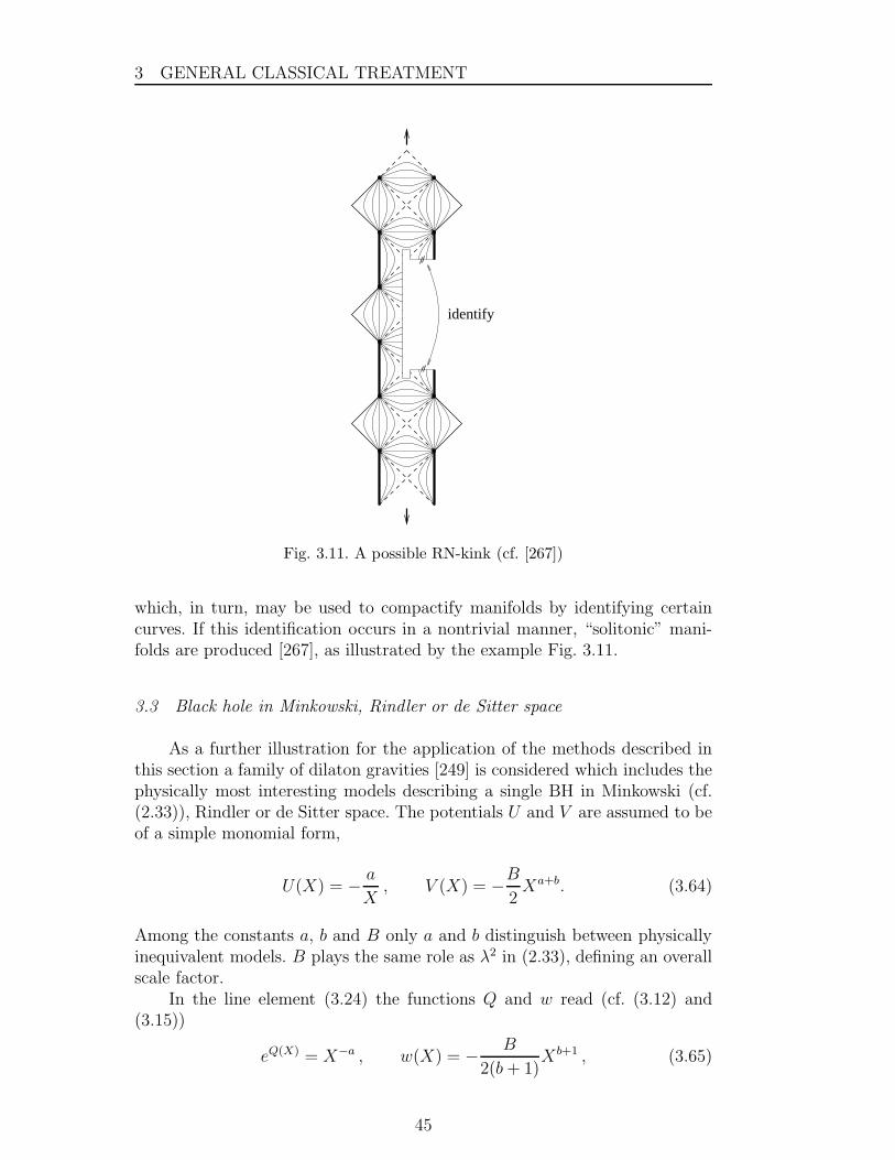
Simple counting of degrees of freedom shows that dilaton gravity withoutmatter fields in 2D has no propagating modes. Therefore, in terms of suitablevariables, the dynamics may be made essentially trivial. This suggests (but inno way guarantees!) that all classical solutions can be found in a closed form.
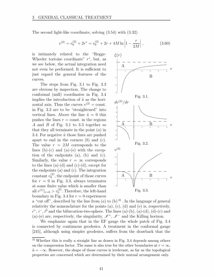
As pointed out already above, the fact that the solutions for dilaton the-ories of type (2.9) can be obtained in analytic form had been tested in manyspecific cases [168, 312,173,391,304,174], always using the conformal gauge
ds2 = 2e2ρdx+dx− (3.1)
or the Schwarzschild gauge (cf. (3.34) below). With (3.1) even for a theory assimple as (2.12) the solution of a Liouville equation
ρ = −Λeρ (3.2)
had been necessary.The advantages of the light cone gauge for Lorentz indices combined with
a temporal gauge for the Cartan variables
e+0 = 0, e−0 = 1, ω0 = 0 (3.3)
was realized first [291] in connection with the classical solution of the KV-model [250]. In this gauge the line element for any 2D gravity theory becomes
(ds)2 = 2e+1 dx1(dx0 + e−1 dx
1) (3.4)
which in GR represents an Eddington-Finkelstein (EF) gauge [134, 156]. Interms of the Killing field kα = (0, 1), the existence of which is a property of thesolutions (∂gµν/∂x
1 = 0) and redefining the x0-coordinate by dx0 = e+1 (x0)dx0,the line element (3.4) may be rewritten as
(ds)2 = dx1(2dx0 + k2dx1) (3.5)
with the Killing norm k2(x0) = kαkα containing all the information of the sys-tem (like ρ(x) in the conformal gauge (3.1)). The key advantage of the ingoing(outgoing) EF gauge as compared to the conformal or the Schwarzschild gaugeis that it is free from coordinate singularities on an ingoing (outgoing) horizon.The only singularities of k2(x0) correspond to singularities of the curvature;zeros k2(x0) = 0 describe horizons. This gauge will turn out to be intimatelyrelated to the natural solution of the e.o.m.-s for all models in the first orderformulation.
In the first subsection 3.1 all classical solutions of GDTs without matterare determined in a very simple way, maintaining gauge invariance. Amongthe specific gauge choices the EF gauge emerges as the most natural one, alsofor the analysis of the global structure of these solutions. The most important
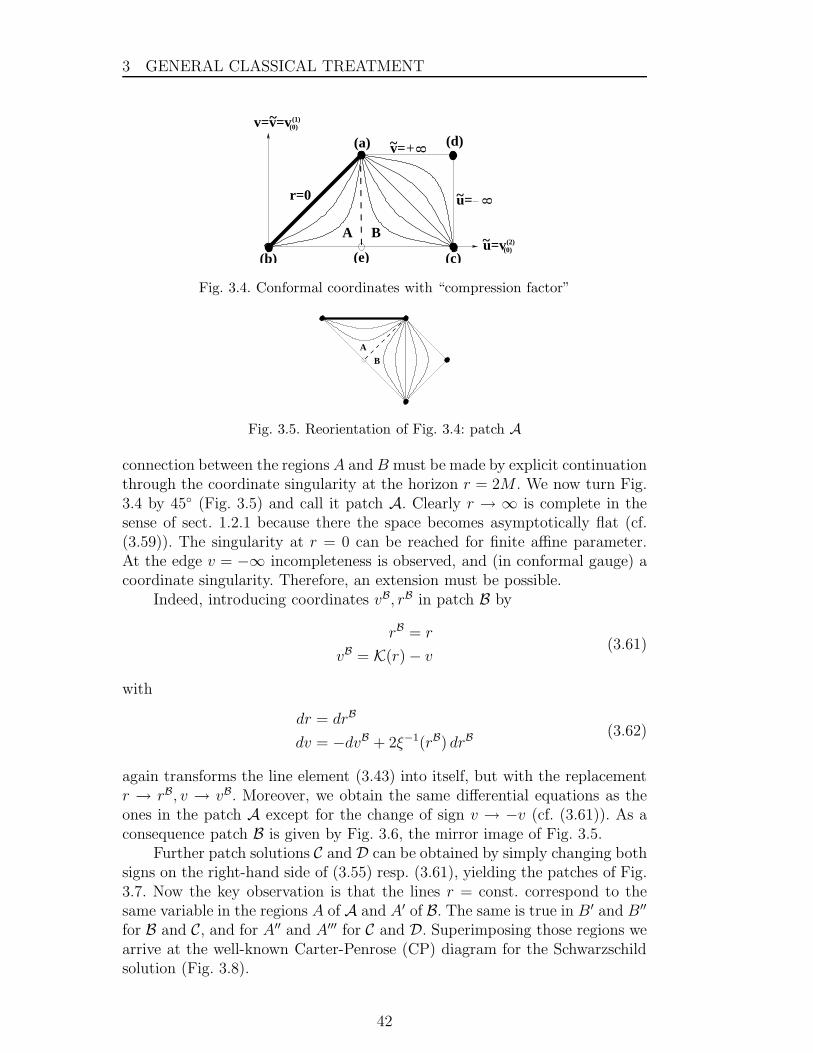
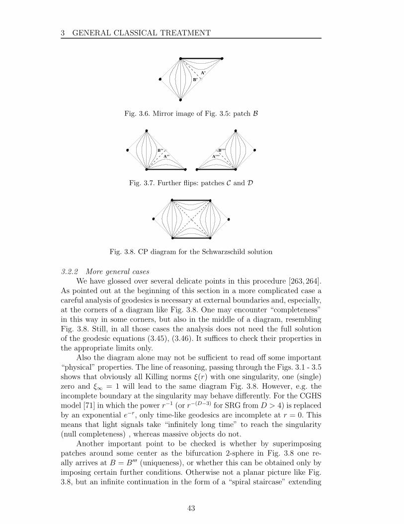
32
3 GENERAL CLASSICAL TREATMENT
dilaton gravity models (cf. fig. 2.1) belong to a two parameter sub-family ofall possible theories. This family of models is considered in more detail in thelast subsection.
3.1 All classical solutions
In anticipation of what we shall need in sect. 4.3 we derive the e.o.m.sfrom an action (2.17) supplemented as L = L(FOG) + L(m) by an, as yet,unspecified matter part L(m). The quantities
W± := δL(m)/δe∓, W := δL(m)/δX (3.6)
contain the couplings to matter. A dependence of L(m) on the spin connec-tion or the auxiliary fields X± will be discarded (cf. sect. 4.3). Variation ofδω, δe∓, δX, and δX∓, respectively, yields the e.o.m.-s
dX +X−e+ −X+e− = 0 , (3.7)
(d± ω)X± ∓ Ve± +W± = 0 , (3.8)
dω + ǫ∂V∂X
+W = 0 , (3.9)
(d± ω)e± + ǫ∂V∂X∓ = 0 . (3.10)
The first equation (3.7) can be used to eliminate the auxiliary fields X± interms of e± and dX. The second pair (3.8) is contained in the set of higher-dimensional Einstein equations for the special case of dimensionally reducedgravity. Eq. (3.9) yields the dilaton current W which is proportional to thetrace of the higher-dimensional energy momentum tensor for dimensionallyreduced gravity, and (3.10) entails the torsion condition. If the potential Vis independent of the auxiliary fields X± the condition for vanishing torsion(1.59) is obtained. Of course, in addition to (3.7)-(3.10) the e.o.m.-s for matterδL(m)/δφA = 0 for generic matter fields φA must be taken into account as well.
In the present section we are interested only in the direct solution of (3.7)-(3.10) without fixing any gauge [290], in the absence of matter (W = W± = 0).Linear combination of the two equations (3.8), multiplied, respectively, by X−
and X+ and using (3.7) leads to (Y = XaXa/2 = X+X−)
d(X+X−) + V(Y,X)dX = 0 . (3.11)
This indicates the existence of a conservation law for a function C(Y,X) =C0 = const. which is nothing else than the Casimir function of the Poisson-Sigma model of sect. 2.3. In the application to physically motivated 2D models,potentials of the form (2.31) were found to be the most important ones. Wetherefore concentrate on those. Multiplying (3.11) by the integrating factorexpQ with
Q =∫ X
U(y)dy, (3.12)
33
3 GENERAL CLASSICAL TREATMENT
one obtains the conservation law
d C = 0 (3.13)
for the Casimir functionC = eQ Y + w (3.14)
with
w(X) =
X∫eQ(y) V (y)dy . (3.15)
Of course, any function of C is also absolutely conserved. Therefore, for somespecific model, among others, a suitable convention must be used to fix thelower limit of integration in Q (influencing an overall factor of C) and thelower limit in (3.15) (yielding an additive overall contribution).
We assume X+ 6= 0 which will be realized (cf. (3.8)) if V (X) = 0 doesnot possess a nontrivial solution for X. This is true in SRG, but e.g. in theKV-model [250] such a “point-solution” may appear for certain values of theparameters [377]. If X+ 6= 0 the first component of eq. (3.8) with a new oneform Z := e+/X+
ω = −dX+
X++ ZV (3.16)
determines the spin connection in terms of the other variables. In a similarway eq. (3.7) may be taken to define e−:
e− =dX
X++X−Z (3.17)
From (3.16) and (3.17) and eq. (3.10) with the upper sign, recalling that now
ǫ = −e−e+ = −dX Z (3.18)
for the potential (2.31), the short relation
dZ − dXZU = 0 (3.19)
follows. The ansatz Z = Z expQ, with the same integrating factor (3.12) as theone introduced above for C, reduces eq. (3.19) to dZ = 0. Now by application ofthe Poincare Lemma (cf. sect. 1.2) Z = df is the only “integration” necessaryfor the full solution 26 :
e+ = X+eQdf (3.20)
e− =dX
X++X−eQdf (3.21)
ω = −dX+
X++ V eQ df (3.22)
C = eQX+X− + w(X) = C0 = const. (3.23)
26 This type of solution has been given first in ref. [377], starting from the Darbouxcoordinates for the KV-model [250].
34
3 GENERAL CLASSICAL TREATMENT
Indeed, all the other equations are easily checked to be fulfilled identically. Eq.(3.23) can be used to express X− in terms X and X+, so that in addition to fbeside the constant C0 we have the free functions X and X+. Eqs. (3.7-3.10)are symmetric in the light cone coordinates. Therefore, the whole derivationcould have started as well from the assumption X− 6= 0.
It is straightforward, although eventually tedious in detail, to generalizethe solution (3.20)-(3.23) to dilaton theories where in (2.9) the factor of theRicci scalar is a more general (non-invertible) function Z(X).
Comparing the number of arbitrary functions (f , X, X+) in the solution(3.20)-(3.23), with the three continuous gauge degrees of freedom, the the-ory is a topological one 27 , albeit of a different type from other topologicaltheories like the Chern-Simons theory [384,385,440,441,442]: there is no dis-crete topological charge like the winding number associated to the solutions.In agreement with sect. 2.3 the only variable which determines the differentsolutions for a given action is the constant C0 ∈ R.
The key role of C is exhibited by the line element
after elimination of X− by (3.23). Whenever a redefinition of X by
dX = dX expQ (3.25)
is possible 28 eq. (3.24) becomes
(ds)2 = 2df ⊗ dX + ξ(X)df ⊗ df , (3.26)
ξ(X) = 2eQ(C0 − w)X=X(X) ; (3.27)
i.e. the EF gauge is obtained when f and X are taken directly as the co-ordinates. Then ξ(X) coincides with the Killing norm k2 (cf. (3.5)). As weshall see in the next subsection the “topological” properties of ξ(X), i.e. thesequence of singularities and zeros (horizons), and the behavior at the bound-aries of the range for X, completely determines the global structure of a so-lution. Eqs. (3.24-3.27), together with the definitions (3.12), (3.15) representthe main result of this section. They are exact expressions for the geometricvariables and thus also for the line element (ds)2 valid for (almost) arbitrarydilaton gravity models without matter. It is now easy to specify other gaugesby taking (3.24) as the point of departure, that is after having solved thee.o.m.-s (3.7)-(3.10) in the simple manner demonstrated above, namely in-serting (x0 = t, x1 = r, F ′ = ∂F/∂r, F = ∂F/∂t)
dX = X ′dr +˙Xdt , df = f ′dr + fdt , (3.28)
27 In the sense that no continuous physical degrees of freedom are present [42].28 If the redefinition is not possible for all X the computation of geodesics shouldstart from (3.24).
35
3 GENERAL CLASSICAL TREATMENT
into (3.26) with (3.27) with appropriate choices for X and f . Of particularinterest are diagonal gauges, a class of gauges to which prominent choices(Schwarzschild and conformal gauge) belong. The absence of mixed terms drdtin the metric can be guaranteed in a certain patch by the gauge conditions
X = X(r) , (3.29)
X ′ + ξf ′ = 0 , (3.30)
and f 6= 0. The solution 29 for f from (3.30)
f = −r∫dx
1
ξ (X(x))· dX(x)
dx+ f(t) =
= −K(X)
2+ f(t) , (3.31)
contains the integral K(X) defined by
K(r) = 2
r∫
r0
dyξ−1(y). (3.32)
The diagonal line element
(ds)2 = ξ[(fdt)2 − (f ′dr)2
], (3.33)
for f = f ′ = 1 attains the form of the conformal gauge. Requiring furthermoredet g = −1 as in Schwarzschild type gauges yields
(ds)2 = ξ(dt)2 − ξ−1(dr)2. (3.34)
As a concrete example we take SRG (2.33) with D = 4, where QSRG =∫X USRG(y)dy = −1/2 lnX with a natural choice y = 1 for the lower limitof integration and wSRG = −2λ2
√X with the lower limit X = 0 (cf.(3.12),
(3.15)). The conserved quantity (3.14) becomes
CSRG =X+X−√X
− 2λ2√X = C0 , (3.35)
and the Killing norm (3.27) reads
k2SRG = ξSRG =
2C0√X
+ 4λ2 . (3.36)
In terms of the new variable X = 2√X the EF gauge (3.26) follows with
ξ(X) = 4C0/X + 4λ2. Further trivial redefinitions (r = X/(2λ), u = 2λf ,
29 f(t) is arbitrary except ˙f 6= 0.
36
3 GENERAL CLASSICAL TREATMENT
dt = du+ dr/ξ) yield the Schwarzschild metric [386]
(ds)2sch =
(1 − 2M
r
)(dt)2 −
(1 − 2M
r
)−1
(dr)2 , (3.37)
where, as expected, C0 is related to the mass M
M = − C0
4λ3. (3.38)
From the steps leading to the line element (3.24) or to one of its subsequentversions it is obvious that these steps can be retraced backwards as easily, sayfrom a Killing norm ξ(X) in (3.27) towards an action. This procedure is notunique, because one function ξ(X) is to be related to two other functions (Uand V ).
For an associated model (2.9) with U = 0, from (3.15) and (3.27) the po-tential V (X) simply results by differentiation dw/dX. However, as emphasizedalready above, these models essentially encode their topology in the parame-ters of the action determined by V (X). In the Killing norm ξ = 2(C0 −w) thevalue of C0 by which the solutions differ in those models only influences theposition of the zeros of ξ, the horizons. For instance, the Reissner-Nordstromsolution of eq. (2.13) follows from the potential anticipated in that equation.As will be seen in sect. 4, when interactions with matter are turned on, C ofthe present chapter is part of the conservation law involving matter contribu-tions. Thus e.g. the influx of matter only changes C and hence in models withU = 0 the position of the horizons, but does not change the “strength” of thesingularities which is fixed here by the mass and the charge Q.
Actually SRG belongs to the interesting class of models in which a givenξ(X) is related to both functions U and V in a very specific way, namely, suchthat C0 = 0 corresponds to a flat (Minkowski) manifold. According to (3.24)this can be simply achieved by the condition
eQw = α = const. , (3.39)
because then the only dependence on X resides in the term ∝ C0 [248]. Thusall models of this class (“Minkowski ground state dilaton theories”) are char-acterized by the relation between U and V in (2.9) following from (3.39):
V (X) =α
2
d
dXexp
−2
X∫U(y)dy
(3.40)
A last related remark concerns the conformal transformation (1.56) of adilaton theory represented by the first order action (2.17). It is always possible,starting from a theory with V (X) and vanishing U(X) to arrive at a model
37
3 GENERAL CLASSICAL TREATMENT
with nonvanishing U(X) by the transformation
ea = ea eQ/2
Xa = Xa e−Q/2
ω = ω +U
2Xa ea
V = e−Q V (X) +XaXa
2U(X) , (3.41)
where Q is defined as in (3.12). In the language of the PSM formulation (sect.2.3) this is an explicit example of a target space diffeomorphism 30 . However, aspointed out already several times, this mathematical transformation connectstwo models with solutions of, in general, completely different topology and/orproperties regarding the role of the conserved quantity C0.
3.2 Global structure
As emphasized in sect. 1.2 the global properties of a solution for thegeometric variables are obtained by following the path of some device onthe manifold. The most important example is the geodesic (1.43) which maypenetrate horizons, but ends when singularities are encountered at finite affineparameter. When no geodesic can reach a boundary of the space-time for finitevalues of the affine parameter the space-time is called geodesically complete,otherwise geodesically incomplete. It should be emphasized that the procedurepresented below does not require the explicit or implicit knowledge of Kruskal-like global coordinates.
For the analysis of the global structure it is convenient to use outgoing oringoing EF coordinates. In a simplified notation [264] the line element (3.26)is written for the outgoing case (f ∝ u, X ∝ r, k2(r) = ξ(r), ξ∞ := +1)
(ds)2out = du(2dr + ξ(r)du) . (3.42)
The ingoing EF gauge (still with ξ∞ = +1)
(ds)2in = dv(2dr− ξ(r)dv) , (3.43)
which will be used here in order to construct patch A of the conformal diagramfor Schwarzschild space-time (see below), could have been obtained if one usesZ := e−/X− for X− 6= 0 in (3.16-3.23). Eq. (3.43) is the most suitable startingpoint for our subsequent arguments in the present example.
For the ingoing metric (xα = v, r)
gµν =
−ξ(r) 1
1 0
(3.44)
30 Cf. the discussion after (2.44).
38
3 GENERAL CLASSICAL TREATMENT
the geodesics (v = v(τ), r = r(τ)) obey
v +v2
2ξ′ = 0 , (3.45)
r − rvξ′ +v2
2ξ′ξ = 0 . (3.46)
These are the e.o.m.-s of (1.42) if the affine parameter τ is identified with s.The Killing field ∂/∂v implies a constant of motion (kα = (1, 0))
gαβkαxβ = r − ξ(r)v =
√|A| = const. (3.47)
which could have been derived as well from (3.46) and (3.45) by taking a properlinear combination. From (3.47) the affine parameter τ can be identified withparameters describing the line-element (3.43)
±(dτ)2 =1
|A|(dr − ξdv)2 = (ds)2 , (3.48)
where the two signs correspond to time-like, resp. space-like geodesics. Thefirst order differential equation
dv
dr=
1
ξ(r)
1 ∓
(1 +
ξ
A
)−1/2 , (3.49)
for the two signs in (3.49) describes two types of geodesics v(1)(r) and v(2)(r)at each point v, r. To avoid confusion with the association of signs, in thenew constant A = ±|A| the two signs from (3.48) have been absorbed so thatnow A > 0 and A < 0 correspond to time-like, resp. space-like geodesics.Inserting (3.49) into (3.48) provides the relation
s(r) = ± 1√|A|
r∫
r0
dy1√
1 + ξ(y)/A. (3.50)
“Special” geodesics A = 0 with
dv
dr= ξ−1(r) , (3.51)
s =
r∫
r0
dy |ξ(y)|−1/2 , (3.52)
and “degenerate” ones obeying A = ξ(r) = const. must be considered sepa-rately.
The advantage of the EF-gauge is visible e.g. in (3.49). The geodesic withthe upper sign in the square bracket clearly passes continuously (C∞) through
39
3 GENERAL CLASSICAL TREATMENT
a horizon where ξ(rh) = 0 which, therefore, does not represent a boundary ofthe patch for the solution (provided A 6= 0).
For a first orientation of the global properties of a manifold it is sufficientto study the behavior of null-directions. Light-like directions are immediatelyread off from (ds)2 = 0 in (3.43):
with K defined in (3.32). In terms of the new variables
v = v(1) , u = v(2) −K(r) (3.55)
those null-directions become the straight lines v = const. u = const.. The lineelement in these (conformal) coordinates, of course, exhibits (coordinate) sin-gularities at the horizons. It should be stressed that conformal coordinates arebeing used here only in order to be in agreement with standard diagrammaticrepresentations.
Furthermore, it is convenient to map (ds)2 by a conformal transformationonto a finite region by considering e.g. [428]
(ds)2 =2dudv ξ(r(u))
(1 + u2)(1 + v2)(3.56)
where the powers of the two factors in the denominator are chosen appropri-ately. Light-like geodesics are mapped onto light-like geodesics, i.e. the causalstructure is not changed by this transformation. The conformal diagrams ob-tained in this way have been introduced by Carter and Penrose [81, 357].
The trivial example is Minkowski space with ξ = 1. From (3.56) with(3.32) and (3.57) both light-cone variables
u = v − 2(r − r0) , v = v (3.57)
lie in −∞ ≤ u, v ≤ +∞. By the compactification (3.56), in the line element
(ds)2 = 2dUdV (3.58)
the new variables U = arctan u, V = arctan v are restricted to the finiteinterval −π/2 ≤ U, V ≤ +π/2.
3.2.1 Schwarzschild metric
As a typical nontrivial example for the general procedure in curved space[264] we take the Schwarzschild BH with
ξ(r) = 1 − 2M
r. (3.59)
40
3 GENERAL CLASSICAL TREATMENT
The second light-like coordinate, solving (3.54) with (3.32)
v(2) = v(2)0 + 2r∗ = v
(2)0 + 2r + 4M ln
∣∣∣∣1 − r
2M
∣∣∣∣ , (3.60)
1 2 3 4 5 6
-3
-2
-1
1
A
ξ(r)
B
r
Fig. 3.1.
1 2 3 4 5 6
-6
-4
-2
2
4
6
8
A
dv(2)/dr
B r
Fig. 3.2.
1 2 3 4 5 6
-5
5
10
15
A
v(2)
B r
Fig. 3.3.
is intimately related to the “Regge-Wheeler tortoise coordinate” r∗, but, aswe see below, the actual integration neednot even be performed. It is sufficient tojust regard the general features of thecurves.
The steps from Fig. 3.1 to Fig. 3.3are obvious by inspection. The change toconformal (null) coordinates in Fig. 3.4implies the introduction of u as the hori-zontal axis. Thus the curves v(2) = const.in Fig. 3.3 are to be “straightened” intovertical lines. Above the line u = 0 thispushes the lines r = const. in the regionsA and B of Fig. 3.1 to 3.3 together sothat they all terminate in the point (a) in3.4. For negative u those lines are pushedapart to end in the corners (b) and (c).The value r = 2M corresponds to thelines (b)-(c) and (a)-(e) with the excep-tion of the endpoints (a), (b) and (c).Similarly, the value r = ∞ correspondsto the lines (a)-(d) and (c)-(d), except forthe endpoints (a) and (c). The integration
constant v(2)0 , the endpoint of those curves
for r = 0 in Fig. 3.3, always terminatesat some finite value which is smaller thanall v(1)|r=0 > v
(2)0 . Therefore, the left-hand
boundary in Fig. 3.4 for r = 0 experiencesa “cut off”, described by the line from (a) to (b) 31 . In the language of generalrelativity the nomenclature for the points (a), (c), (d) and (e) is, respectively,i+, i−, i0 and the bifurcation-two-sphere. The lines (a)-(b), (a)-(d), (d)-(c) and(a)-(e) are, respectively, the singularity, I +, I − and the Killing horizon.
We emphasize again that in the EF gauge the whole patch of Fig. 3.4is connected by continuous geodesics. A treatment in the conformal gauge[245], although using simpler geodesics, suffers from the drawback that the
31 Whether this is really a straight line as drawn in Fig. 3.4 depends among otherson the compression factor. The same is also true for the other boundaries at r = ∞,u = −∞. However, the shape of those curves is irrelevant, as far as the topologicalproperties are concerned which are determined by their mutual arrangement only.
41
3 GENERAL CLASSICAL TREATMENT
u=
v=
~u=vA B
r=0
(a)
~
~
v=v=v~
(c)(b)
(0)(1)
(0)(2)
(e)
(d)
8
8+
Fig. 3.4. Conformal coordinates with “compression factor”
A
B
Fig. 3.5. Reorientation of Fig. 3.4: patch A
connection between the regions A andB must be made by explicit continuationthrough the coordinate singularity at the horizon r = 2M . We now turn Fig.3.4 by 45 (Fig. 3.5) and call it patch A. Clearly r → ∞ is complete in thesense of sect. 1.2.1 because there the space becomes asymptotically flat (cf.(3.59)). The singularity at r = 0 can be reached for finite affine parameter.At the edge v = −∞ incompleteness is observed, and (in conformal gauge) acoordinate singularity. Therefore, an extension must be possible.
Indeed, introducing coordinates vB, rB in patch B by
rB = r
vB = K(r) − v(3.61)
with
dr = drB
dv = −dvB + 2ξ−1(rB) drB(3.62)
again transforms the line element (3.43) into itself, but with the replacementr → rB, v → vB. Moreover, we obtain the same differential equations as theones in the patch A except for the change of sign v → −v (cf. (3.61)). As aconsequence patch B is given by Fig. 3.6, the mirror image of Fig. 3.5.
Further patch solutions C and D can be obtained by simply changing bothsigns on the right-hand side of (3.55) resp. (3.61), yielding the patches of Fig.3.7. Now the key observation is that the lines r = const. correspond to thesame variable in the regions A of A and A′ of B. The same is true in B′ and B′′
for B and C, and for A′′ and A′′′ for C and D. Superimposing those regions wearrive at the well-known Carter-Penrose (CP) diagram for the Schwarzschildsolution (Fig. 3.8).
42
3 GENERAL CLASSICAL TREATMENT
A’
B’
Fig. 3.6. Mirror image of Fig. 3.5: patch B
B’’A’’ A’’’
B’’’
Fig. 3.7. Further flips: patches C and D
Fig. 3.8. CP diagram for the Schwarzschild solution
3.2.2 More general cases
We have glossed over several delicate points in this procedure [263, 264].As pointed out at the beginning of this section in a more complicated case acareful analysis of geodesics is necessary at external boundaries and, especially,at the corners of a diagram like Fig. 3.8. One may encounter “completeness”in this way in some corners, but also in the middle of a diagram, resemblingFig. 3.8. Still, in all those cases the analysis does not need the full solutionof the geodesic equations (3.45), (3.46). It suffices to check their properties inthe appropriate limits only.
Also the diagram alone may not be sufficient to read off some important“physical” properties. The line of reasoning, passing through the Figs. 3.1 - 3.5shows that obviously all Killing norms ξ(r) with one singularity, one (single)zero and ξ∞ = 1 will lead to the same diagram Fig. 3.8. However, e.g. theincomplete boundary at the singularity may behave differently. For the CGHSmodel [71] in which the power r−1 (or r−(D−3) for SRG from D > 4) is replacedby an exponential e−r, only time-like geodesics are incomplete at r = 0. Thismeans that light signals take “infinitely long time” to reach the singularity(null completeness) , whereas massive objects do not.
Another important point to be checked is whether by superimposingpatches around some center as the bifurcation 2-sphere in Fig. 3.8 one re-ally arrives at B = B′′′ (uniqueness), or whether this can be obtained only byimposing certain further conditions. Otherwise not a planar picture like Fig.3.8, but an infinite continuation in the form of a “spiral staircase” extending
43
3 GENERAL CLASSICAL TREATMENT
Fig. 3.9. Basic patch of Reissner-Nordstrom metric
Fig. 3.10. Penrose diagram for Reissner-Nordstrom metric
above (and below) the drawing plane may emerge.When ξ exhibits two zeros as for the Reissner-Nordstrom metric
ξRN = 1 − 2M
r+Q2
r2(3.63)
the basic patch of Fig. 3.9 with the superposition method described above,leads to the well-known [234,265] one-dimensional infinite periodic extensionof Fig. 3.10.
When even three zeros are present in the Killing norm the global diagrambecomes periodic in two directions (cf. e.g. Fig. 2.1-2.3 in [197]), i.e. coversthe whole plane 32 .
Such one, two or more dimensional lattices exhibit discrete symmetries,
32 Here we have even discarded the “uniqueness”-problem, referred to above.
44
3 GENERAL CLASSICAL TREATMENT
identify
Fig. 3.11. A possible RN-kink (cf. [267])
which, in turn, may be used to compactify manifolds by identifying certaincurves. If this identification occurs in a nontrivial manner, “solitonic” mani-folds are produced [267], as illustrated by the example Fig. 3.11.
3.3 Black hole in Minkowski, Rindler or de Sitter space
As a further illustration for the application of the methods described inthis section a family of dilaton gravities [249] is considered which includes thephysically most interesting models describing a single BH in Minkowski (cf.(2.33)), Rindler or de Sitter space. The potentials U and V are assumed to beof a simple monomial form,
U(X) = − a
X, V (X) = −B
2Xa+b. (3.64)
Among the constants a, b and B only a and b distinguish between physicallyinequivalent models. B plays the same role as λ2 in (2.33), defining an overallscale factor.
In the line element (3.24) the functions Q and w read (cf. (3.12) and(3.15))
eQ(X) = X−a , w(X) = − B
2(b+ 1)Xb+1 , (3.65)
45
3 GENERAL CLASSICAL TREATMENT
so that
(ds)2 = X−adf ⊗[2dX + 2
(C0 +
B
2(b+ 1)Xb+1
)df
]. (3.66)
The equation w = C0 has at most one solution on the positive semi-axis. Hencethe metric (3.66) exhibits at most one horizon.
The most interesting models correspond to positive a for which the func-tion X−a diverges at X = 0. For X > 0 in terms of the alternative definitionof the dilaton field Φ (2.11) the dilaton action (2.10) with the potentials (3.64)becomes
L(dil) =1
2
∫d2x
√−ge−2Φ[R + 4a(∇Φ)2 −Be2(1−a−b)Φ
], (3.67)
which may be more familiar to a string audience.It is also instructive to calculate the scalar curvature:
R = 2aC0Xa−2 +
Bb
b+ 1(b+ 1 − a)Xa+b−1 . (3.68)
In what follows only models with b 6= −1 will be considered (although b = −1can be analyzed too [249]). For the “ground state” solutions C0 = 0 only thesecond term in (3.68) survives. If a = b + 1 or b = 0 the scalar curvature ofthe ground state is zero. A more detailed analysis shows that the first case(a = b+1) corresponds to Minkowski space, and the second (b = 0) to Rindlerspace. The condition a = b + 1 for the Minkowski ground state models alsofollows from (3.40). If a = 1 − b the ground state has constant curvature andcorresponds to (anti-) de Sitter space.
For the general solutions (3.66) with C0 6= 0 it follows from (3.68) that,depending on the values of a and b, they may show a curvature singularity atX = 0, at X = ∞, or at both values. In the special cases considered abovethere could be only one singularity. Therefore, these models describe (in asomewhat generalized sense) a single BH immersed in Minkowski, or Rindler,or de Sitter space.
Many interesting and important models belong to the two-parameter fam-ily of this section. The SRG models (2.2) for general dimension D lie on theline a = b + 1 between a = 1/2 (this point corresponds to D = 4) and a = 1.As D grows, these models approach the point a = 1, corresponding to theCGHS model [71]. The point a = 0, b = 1 describes the Jackiw-Teitelboimmodel [22,405,238]. Lemos and Sa [298] gave the global solutions for b = 1−a,Mignemi [323] considered a = 1 and all values of b. The models of [148] cor-respond to b = 0 and a ≤ 1. The general solution for the whole plane wasobtained in ref. [249] and is summarized in Fig. 3.12.
In order to calculate quantities like the ADM mass and the Hawking fluxit is essential to re-write the line element (3.66) for asymptotically Minkowski,de Sitter and Rindler models in such a form that it becomes the standard one
46
3 GENERAL CLASSICAL TREATMENT
b
10 a2
1
at singularity
incomplete
null
SBH
b=a-1
Fig. 3.12. “Phase” diagram showing the CP diagrams related to the (a- andb-dependent) action (3.67). Bold lines in those diagrams denote geodesically in-complete boundaries. Spherically reduced models lie on the half-line b = a − 1,b ≤ 0, the endpoint of which corresponds to CGHS. The special case of SRG fromD = 4 is depicted by the point labelled by SBH.
in the asymptotic region. Here we give an explicit expression for the asymptot-ically Minkowski solutions only (other cases can be found in ref. [299]) wheresuch a representation is possible for a ∈ (0, 2). We repeat the steps which ledbefore from the metric (3.24) to the Schwarzschild black hole (3.37). Namely,we first introduce the coordinates X = r, f = u (cf. (3.26))
u =
√B
af sign(1 − a) , r =
√a
B
1
|1 − a|X1−a (3.69)
and write the metric in EF form (3.27) where ξ now reads
ξ (r) = 2C0 |1 − a| aa−1 r
aa−1
(B
a
) 2−a2(a−1)
+ 1 (3.70)
Following the steps after (3.28) one arrives at the generalized Schwarz-schild metric (3.34) with ξ as in (3.70).
For a ∈ (0, 1) the asymptotic region corresponds to r → ∞, while for
47
3 GENERAL CLASSICAL TREATMENT
a ∈ (1, 2) it is reached with the limit r → 0. In both cases ξ(r) → 1, and themetric assumes the standard Minkowski form gµν → diag(1,−1).
For the asymptotically Rindler and de Sitter solution with a belonging tothe same interval, a ∈ (0, 2), the quantity ξ becomes
ξ(r) = rB122 −Mr
aa−1 (3.71)
for the Rindler solutions, and
ξ(r) = r2B2 −Mra
a−1 (3.72)
for the de Sitter solutions. Explicit expressions for the constants M and B2
and for the variables t and r can be found in ref. [299]. The presence of typicallinear (Rindler) and quadratic (de Sitter) terms in (3.71) and (3.72) shouldbe noted.
Although the CGHS model a = 1, b = 0 belongs to the family of theasymptotically Minkowski models considered above, the equations (3.69) aresingular at a = 1. Appropriate coordinates for this case are
u = −√Bf , r = − 1√
BlnX . (3.73)
The line element (3.27) now contains
ξ(r) = 1 +2C0e
√Br
B. (3.74)
A somewhat non-standard feature of (3.74) is that the asymptotic region issituated at r → −∞.
48
4 ADDITIONAL FIELDS
4 Additional fields
In 2D there are neither gravitons nor photons, i.e. no propagating physicalmodes exist [42]. This feature makes the inclusion of Yang-Mills fields in 2Ddilaton gravity or an extension to supergravity straightforward. Indeed, bothgeneralizations can be treated again as a PSM (2.34) with generalized AI andXI . More locally conserved quantities (Casimir functions) may emerge andthe integrability concept is extended.
Beside gauge fields also scalar and spinor fields may be added. If the latterare derived from higher dimensions through spherical reduction they are non-minimally coupled to the dilaton. The introduction of those fields in generaldestroys the integrability. Only in special cases exact solutions still can beobtained. An example are chiral fermions [278] or (anti-)selfdual scalars [356].
4.1 Dilaton-Yang-Mills Theory
The interaction with additional one-form Yang-Mills fields Aa related tolocal gauge transformations belonging to a compact Lie group G is simply in-cluded in (2.17) by introducing further auxiliary variables Za (additional tar-get space coordinates in the PSM language) in the dilaton-Yang-Mills (DYM)action
contains the structure constants fabc and the gauge coupling g. The potentialV, invariant under local Lorentz transformations and transformations G nowalso may depend on the Casimir invariants ci of the group G. For instancein G = SU(N) there are N − 1 independent invariant polynomials of degree2, 3, . . . , N − 1 in terms of the components Za.
The abelian case (f = 0 in (4.2)) is especially simple. There V onlydepends on the single variable Z. Variation of (4.1) with respect to A directlyyields dZ = 0, i.e. Z = Z0 = const is conserved, an additional Casimir functionin the PSM-interpretation of (4.1). Because Z = Z0 is the result of solving adifferential equation it cannot be simply reinserted into (4.1). Variation of Zyields
dA = −ǫ ∂V∂Z
∣∣∣∣∣Z=Z0
. (4.3)
The remaining e.o.m-s can be solved as for (2.17) by (3.20-3.23) with just anadditional dependence on the constant Z = Z0 in the potential V in (3.22)
49
4 ADDITIONAL FIELDS
and in w(X,Z) of (3.23) [289, 305].For a nonabelian gauge group G the coupling between the gauge fields
Aa and the geometric variables is somewhat more complicated, but as a PSMit can be treated again along the lines of sect. 3.1. For a potential of thetype V(X+X−, X) + α(X)ZaZa the solution of the geometric sector can beobtained like the one from of an ordinary GDT, because ZaZa is constanton-shell [263, 264, 397]. Such a potential correctly reproduces the e.o.m.-s forordinary D=2 dilaton-Yang-Mills theory:
(DA)a = −ǫα(X)Za , d(ZaZa) = 0 (4.4)
Some explicit solutions for the dilaton-Maxwell-Scalar system can be found inref. [353].
The action (4.1) does not contain the special case which emerges fromspherical reduction of Einstein-Yang-Mills (EYM) in D = 4. The reasonfor this is obvious: While the Killing vectors ξs associated with sphericalsymmetry act trivially on the metric, δξsgµν = 0 with δξs being the Lie-derivative with respect to ξs, a corresponding transformation of the gauge fieldAµ → Aµ − εsδξsAµ can be compensated by a suitable gauge transformation,Aµ → Aµ + εsDµWs, such that δξsAµ = DµWs [162]. Already for SU(2) themost general solution compatible with spherical symmetry, sometimes called“Witten’s ansatz” [438], yields terms which are not described by (4.1), namelyan additional (minimally coupled) charged scalar field with dilaton-dependentmass term and quartic self-interaction 33 .
4.2 Dilaton Supergravity
Already a long time ago the superfield approach has been applied insupersymmetric extensions of GDTs [223]. Superfields are expressed in termsof supercoordinates zM = (xm, θµ), where the bosonic coordinates xm aresupplemented 34 by anticommuting (Grassmann) coordinates θµ.
We assume the latter to be Majorana spinors, i.e. we restrict ourselves toN = 1 superspace inD = 2. Beside the Z2-grading property for coordinates 35 ,
zMzN = (−1)MNzNzM , (4.5)
33 Cf. [427] for a comprehensive review on non-trivial EYM solutions.34 Throughout this subsection we employ the generally accepted supersymmetrynotation with Latin indices from the middle of the alphabet for the holonomicbosonic coordinates xn (denoted “xµ” in the rest of this Report). Greek indices arereserved for the fermionic coordinates θµ. A similar notation is used in tangentialspace for Lorentz vectors XA = (Xa,Xα) with indices from the beginning of thealphabet.35 In the exponent of (−1), M or N is zero for a bosonic component, for a fermionicone M resp. N are 1.
50
4 ADDITIONAL FIELDS
the derivatives with respect to z are defined to act to the right→
∂M =→
∂/∂zM .Only those derivatives will appear in the following, so the arrow will bedropped.
Any vector-field in superspace V = V M∂M is invariant under non-degen-erate coordinate changes zM → zM (z)
V M∂M = V M ∂zL
∂zM∂zN
∂zL∂
∂zN, (4.6)
which shows the advantage of the conventional summation of indices “ten tofour” in supersymmetry, already introduced in the section on PSM-s (sect.2.3).
Now any formula of differential geometry in ordinary space of the PSMcan be copied to superspace notation. The p-forms eq. (1.14), of sect. 1.2.1turn into the same expressions written in terms of dzM instead of dxµ, adheringstrictly to the summation of supersymmetry:
Φ =1
p!dzMp ∧ · · · ∧ dzM1ΦM1···Mp
(4.7)
Also the external differential is defined in agreement with sect. 2.3 as
dΦ =1
p!dzMp ∧ · · · ∧ dzM1 ∧ dzN∂NΦM1···Mp
(4.8)
which implies the Leibniz rule (2.37) for superforms, already introduced in thatsection in anticipation of the graded PSM (gPSM) approach below. Clearlythe (anti-)symmetry properties of the tensor ΩM1 ...Mp
now depend on thegraded commutation properties (4.5) of the indices. Instead of (1.13), (1.14)the one-forms of superzweibein and superconnection are EM
A and
ΩMAB = ΩMLA
B , (4.9)
where in (4.9) the simplification for two dimensions with
LAB =
ǫab 0
0 −12(γ∗)α
β
(4.10)
already has been taken into account. The fermionic part in (4.10), the gener-ator of Lorentz transformations in spinor space, agrees with (1.61). Covariantderivatives, defined by analogy to (1.23)
∇MVA = ∂MV
A + ΩMVBLB
A ,
∇MVA = ∂MVA − ΩMLABVB .
(4.11)
lead to the expressions for the components of supercurvature and supertorsion
RMNAB =
(∂MΩN − ∂NΩM(−1)MN
)LA
B =: FMNLAB, (4.12)
51
4 ADDITIONAL FIELDS
TMNA = ∂MEN
A + ΩMENBΩMLB
B − (M ↔ N)(−1)MN (4.13)
Again Bianchi identities, direct generalizations of (1.26) and (1.28), must hold(cf. [142], eqs. (1.58), (2.20)). They restrict the component fields, contained inEM
A,ΩM when these expressions are expanded in terms of (a finite numberof) ordinary fields, appearing as coefficients of powers Θµ and Θ2 = ΘµΘµ.It turns out that to deal with supertorsion it is more convenient to use itsanholonomic components:
TABC = (−1)A(B+N) EB
NEAMTMN
C (4.14)
The literature on 2D supergravity (cf. e.g. [223,60,315,370,368,297]) is stronglyinfluenced by its close relation to string theory, where the bosonic torsion van-ishes, Tab
c = 0. It uses the further constraints on TABC
Tαβc = 2i (γc)αβ, Tαβ
γ = 0 , (4.15)
the first of which is dictated by the requirement that in the limit of globaltransformations ordinary supersymmetry should be restored. The second oneturns out to be a convenient choice, because then the Bianchi identities in aWess-Zumino type gauge are fulfilled identically [141].
In the application to 2D gravity including bosonic torsion it seems nat-ural to retain (4.15), but to simply drop the zero bosonic torsion condition.However, as a consequence of the Bianchi identities it turned out [141] that thesuperfield components, obtained in this manner, did not permit the construc-tion of 2D supergravity Lagrangians with nonvanishing bosonic torsion, afterall. Only after replacing (4.15) by the weaker set (Fαβ = Eα
M EβN FNM(−1)M ,
cf. (4.12))
(γa)βα Tαβ
c = −4iδac, Tαβ
γ = 0, (γa)βαFαβ = 0 (4.16)
a solution can be found [142]. However, the mathematical complexity of thisapproach becomes considerable.
Instead, we turn to the generalization of the PSM, adding fermionic targetspace coordinates χα and corresponding Rarita-Schwinger 1-form fields ψα tothe degrees of freedom in (2.34), (2.38) as 36
XI = (X,Xa, χα) ,
AI = (ω, ea, ψα) .(4.17)
Apart from that, the PSM action retains the form (eq. (2.34)).
36 Under the title “free differential algebras” this has been proposed for simplemodels in ref. [237], cf. also refs. [228,229,398].
52
4 ADDITIONAL FIELDS
Both χα and ψα denote Majorana fields, when, as in what follows, N = 1supergravity is considered 37 . The graded Poisson tensor PIJ = (−1)IJ+1PJI
instead of (eq. (2.36)) is now assumed to fulfill a graded Jacobi identity
PIL→
∂LPJK + gcycl(IJK) = 0 . (4.18)
Except for the range of fields to be summed over, the e.o.m-s are again (2.41),(2.42). The symmetries (2.43), (2.44) depend on infinitesimal local parametersǫI = (ǫφ, ǫa, ǫα).
The mixed components PαX are constructed by analogy to PaX in (2.39)with the appropriate generator (−γ∗/2) of Lorentz transformations in 2Dspinor space (cf. eq. (4.10)). Then dǫα in the second set of eq. (2.44) acquiresan additional term casting it into the covariant combination (Dǫ)α, with co-variant derivative (1.63). This is precisely the form required for the (dilatondeformed) supergravity transformation of the “gravitino” ψα. As the Poissontensor PIJ also here is not of full rank, Casimir functions C(Y, φ, χ2) existwhich, following the same line of argument as in sect. 2.3 obey dC = 0. FromLorentz invariance a bosonic C in supergravity is of the form
C = c+ 12χ2c2 , (4.19)
where c coincides with the quantity denoted by C in the pure bosonic case(2.46,3.23). However, also fermionic Casimir functions may appear (see below).
The determination of all possible minimally extended supergravities re-duces to the solution of the Jacobi identities (4.18). In the general ansatz forPIJ
Pab = V ǫab , (4.20)
Pbφ = Xa ǫab , (4.21)
Pαφ = −1
2χβ(γ∗)β
α , (4.22)
Pαb = χβ(F b)βα , (4.23)
Pαβ = vαβ +χ2
2vαβ2 , (4.24)
the function
V = V(X, Y ) +χ2
2v2(X, Y ) (4.25)
contains the original bosonic potential V. As explained above, eqs. (4.21) and(4.22) are fixed completely by Lorentz invariance. This invariance also impliesthat the (symmetric) spinor-tensor V αβ in (4.24) can be expanded furtherinto three scalar functions of X and Y , multiplying the symmetric matrices
37 In higher N supergravity Majorana fields(1)
χα · · ·(N)
χα and corresponding(i)
ψα areneeded with an additional SO(N) symmetry.
53
4 ADDITIONAL FIELDS
(γ∗)αβ, γαβa , Xa(γ∗γa)
αβ:
V αβ = Uγ∗αβ + i UXaγaαβ + i UXaǫa
bγbαβ =
= vαβ +χ2
2vαβ2 .
(4.26)
Each function U again has a pure bosonic part and, as indicated in the secondline of (4.26), a term proportional to χ2. In a similar manner the spinor F b
in (4.23) can be expressed in terms proportional to δβα, (γa)β
α(γ∗)βα which
finally requires eight scalar functions of X and Y , multiplied by appropriatefactors constructed with the help of Xa and ǫab [140]. In (4.23) the multiplyingfactor χ precludes terms with factor χ2 in F . Thanks to (4.21) and (4.22) theJacobi identities with one index referring to X are fulfilled automatically. Theremaining ones can be solved algebraically, provided a quite specific sequenceof steps is followed (for details see [140]). Three main cases are determined bythe rank of the 2 × 2 spinor matrix vαβ in (4.26).
For full rank (det vαβ 6= 0) the solution is found to depend on five scalarfunctions of X, Y and the derivatives thereof, if the bosonic potential V in(4.25) is assumed to be given.
If the fermionic rank is reduced, beside the bosonic Casimir function(4.19) one or two fermionic ones exists. They are of the generic form
C(±) = χ±∣∣∣∣∣X−−
X++
∣∣∣∣∣
±1/4
c(±) (X, Y ) (4.27)
and owe their Lorentz invariance to the interplay of the abelian boost trans-formations exp(±β) of the light cone coordinates X±± related to Xa, andexp(±β/2) of the chiral spinor components χ± of χα. For fermionic rank 1 thegeneral solution contains four arbitrary functions beside V and one additionalCasimir function of type (4.27). For rank zero of the fermionic extension inPIJ beside (4.19) both fermionic Casimir functions (4.27) are conserved andthree functions remain arbitrary for a given bosonic potential.
In order to avoid solving differential equations by imposing the Jacobiidentities (4.18) also for reduced fermionic rank, it is important to make in-tensive use of the information on the Casimir functions.
The arbitrariness of the solution of the Jacobi identities can be under-stood as well by studying reparametrizations of the target space, spanned bythe XI in the gPSM. Those reparametrizations may generate new models.Therefore, they can be useful to create a more general gPSM from a simplerone, although this approach is difficult to handle if V in (4.25) is assumed tobe the given starting point. However, the subset of those reparametrizationsmay be analyzed which leaves a given bosonic theory unchanged. Again thesame number of arbitrary functions emerges for the different cases describedin the paragraphs above.
As an illustration we quote eq. (4.252) from [140] which represents one (ofmany) supergravity actions which possess a bosonic potential (2.31) quadratic
54
4 ADDITIONAL FIELDS
in torsion 38 :
L(QBT) =∫
MXdω +XaDea + χαDψα + ǫ
(V + 1
2XaXaU + 1
2χ2v2
)
+U
4Xa(χγ3γaγ
bebψ) − i V
2u(χγaeaψ)
− i
2Xa(ψγaψ) − 1
2
(u+
U
8χ2)
(ψγ3ψ),
v2 = − 1
2u
(V U + V ′ +
V 2
u2
).
(4.28)
In this formula U(X) is the quantity defined in (2.31). The prepotential u isrelated to U(X) and V (X) by
u2(X) = −2 e−Q(X) w(X) , (4.29)
where Q and w have been defined in (3.12) and (3.15).The supergravity transformations of ea and ψα with small fermionic pa-
rameter ǫ for this action (4.28)(cf. eqs. (4.255) - (4.259) of [140] and footnote38) are of the form
Thus, they contain the essential terms, but, not shown here, also others, be-cause of the deformation by the dilaton field. SRG is the special case (2.33)for U and V , but as a supergravity extension (4.28) is not unique.
A generic property of the fermionic extensions obtained in this analysis isthe appearance of obstructions, which is a typical feature of supersymmetrictheories (cf. e.g. [133]). The first type of those consists in singular functions ofthe bosonic variables X and Y , multiplying the fermionic parts of a supergrav-ity action, when no such singularities are present in the bosonic part. But evenin the absence of such additional singularities, a relation like (4.29) betweenthe original potential and some prepotential u, dictated by the correspondingsupergravity theory, either leads to a restriction of the range of X and/or Yas given by the original bosonic one, or even altogether prevents any exten-sion of the latter. Remarkably, a known 2D supergravity model like the oneof Howe [223] which originally had been constructed with the full machineryof the superfield technique, is one example which escapes such obstructions.There, in our language, the PSM potential V = −2λ2X3 permits an expansionin terms of the prepotential u(X) through V = −du2/dX because Q = 0. Anexample where obstructions seem to be inevitable is the KV-model [250] withquadratic bosonic torsion.
On the other hand, the supergravity extension of SRG following from theaction (4.28) is free from such problems. However, it is not the only possible
38 We comply with our present notation by the replacements φ→ X,Z → U(X) inref. [140]. Furthermore an arbitrary constant is now fixed as u0 = 1.
55
4 ADDITIONAL FIELDS
extension of the bosonic theory. Indeed, the hope that a link could be foundbetween the possibility of reducing the arbitrariness of extensions referred toabove, and of the absence of such obstructions, did not materialize. Severalcounter examples could be given including different singular and nonsingularextensions of SRG.
Another very important point concerns the “triviality” of supergravityextensions, proved earlier by Strobl [398]. It was based upon the observationthat locally a formulation of the dynamics in terms of Darboux coordinatesallows to elevate the infinitesimal transformations (2.43,2.44) (on-shell) to fi-nite ones. Then the latter may be used to gauge the fermionic fields in 2Dsupergravity to zero. Providing now the explicit form of those Darboux coor-dinates in the explicit solution of a generic model, additional support has beengiven to the original argument of ref. [398]. However, the appearance of theobstructions and the ensuing singular factors in the transition to the Darbouxcoordinates may introduce a new aspect. When those new singularities ap-pear at isolated points without restriction of the range for the original bosonicfield variable, they may be interpreted and discarded much like coordinatesingularities. Another way to circumvent this problem in the presence of re-strictions to the range and thus to retain triviality is to allow a continuationof our (real) theory to complex variables. This triviality disappears anyhow,when interactions with additional matter fields are introduced, obeying thesame symmetry as given by the gPSM-theory. A proposal in this direction canbe found in ref. [237].
In order to eliminate the arbitrariness of superdilaton extensions the onlyviable argument seems to start from a supergravity theory in higher dimen-sions (e.g. D = 4) and to reduce it (spherically or toroidally) to a D = 2effective theory. It turns out that the Killing spinors needed in that case mustbe Dirac spinors, requiring the generalization of the work of ref. [140] to (atleast) N = 2, where, however, the same technique of gPSM-s can be applied.
As in the bosonic case an action like (4.28) or, better, directly its gPSMform (2.34) can be converted into a dilaton theory by elimination of the torsiondependent part of the spin connection and of Xa. Also for supergravity theequation for Xa is independent of the potential V, eq. (2.29) being replacedby
Xa = −eamǫmn[(∂nX) +1
2(χγ∗ψn)] . (4.31)
The corresponding dilaton action in the gPSM notation becomes
L =∫
M
[Xdω + χα(Dψ)α +1
2PAB |Xa eB eA ] , (4.32)
where ω is the torsionless part of the curvature as in (2.27) and |Xa meansthat the components of the Poisson tensor (in the anholonomic basis) are tobe taken with Xa given by (4.31). When (4.32) is written in components (cf.eq. (4.246) of [140]) with the bosonic potential (2.31) for the Howe model
56
4 ADDITIONAL FIELDS
(V = −12X3, U = 0), it can be checked that the superdilaton theory, obtained
in this way differs from the direct superextension of the bosonic theory [354].The reason is that in our approach X is directly promoted to be the bosoniccomponent of the superfield, whereas in ref. [354] the dilaton represents thebosonic part of yet another scalar superfield.
4.3 Dilaton gravity with matter
4.3.1 Scalar and fermionic matter, quintessence
For the inclusion of scalar matter as in sect. 2.1 we start with the ex-ample of spherical reduction of Einstein theory. When massless scalar fieldsare coupled minimally in D dimensions ((∇(D)Φ)2 = gMN∂MΦ ∂NΦ ; M,N =0, 1, . . . D − 1)
L(m,D)(φ) =
1
2
∫dDx
√−g(D) (∇(D)Φ)2 , (4.33)
for scalar fields φ = φ(x0, x1) the 2D reduced action in terms of the compo-nents of gMN as derived from the line-element (2.1), becomes
L(m)(φ) =
OD−2
λD−2
∫d2x
√−g F (X) (∇φ)2 , (4.34)
FSRG(X) =X
2. (4.35)
Such an interaction is an example of nonminimal coupling (F (X) 6= const.) inthe reduced case. Admitting a general function F (X), a dilaton field depen-dence different from SRG (eq. (4.35)) can be covered as well. An especiallysimple theory follows for F = const., minimal coupling at the D = 2 level 39 .Below we shall absorb the relative factor 1/2 between the dilaton action (2.2)and the first order action (2.17) – which of course must also be adjusted prop-erly in the matter action – into the coupling function F (X).
Dropping as in our convention for the geometrical part of the FOG actionin (2.17) the prefactor 2OD−2/λ
D−2, the action (4.34) can be written also as
L(m)(φ) =
1
2
∫
M2
F dφ ∗ dφ =1
2
∫F (dφea) ∗ (dφeb) ηab . (4.36)
In order to avoid the delicate subject of Killing spinors, necessary forthe (spherical) reduction of fermions 40 (cf. e.g. [358] for D = 4) we shallonly deal with fermions introduced directly in D = 2. The diffeomorphism
39 This is not to be confused with F ∝ X, corresponding to minimal coupling in theoriginal dimension in the case of SRG. We will refer to that case as non-minimalcoupling.40 Such a reduction yields a dilaton dependent “mass” term and coupling of spinorsto the auxiliary fields X±.
57
4 ADDITIONAL FIELDS
covariant generalization (cf. (1.63)) of the Dirac action
L(m)(ψ) =
i
4
∫d2x
√−g eµa (ψγa↔D
(ψ)
µ ψ) (4.37)
as in Minkowski space must contain a two-sided derivative a↔Db = a(Db) −
(Da)b in order to yield a real action. The cancellation of ω in that derivative
is a peculiar feature of D = 2, i.e. the simplification↔Dµ =
↔∂µ is possible
there. Thus both interactions (4.36) and (4.37) do not depend on the spinconnection, as anticipated already in deriving the (classical) e.o.m.-s withmatter, eqs. (3.6)-(3.10).
An additional geometrical degree of freedom may also appear already atthe D = 4 level. Recently in connection with the observation of supernovaeat high values of the redshift [367, 365, 366, 359] the validity of the Hilbert-Einstein theory has been put into doubt [12]. The simplest theoretical descrip-tion requires the introduction of a (still very small) cosmological constant Λ(de Sitter theory). Therefore, extensions of the Einstein theory towards theold Jordan-Brans-Dicke (JBD) theory [153,241,51], have been revived, wherealready at D = 4 an additional scalar field Φ (Jordan field, “quintessence”) isassumed to exist [433,431,80,447,363]. Then, already in D = 4 an action like(2.9) is postulated with X → Φ and appropriate assumptions for functionsU(4)(Φ), V(4)(Φ) so that the “effective cosmological constant” is driven to itspresent (small) value 41
L(Q) =∫d4x
√−g(4)
[R(4) Φ + U(4)(Φ) (∇(4)Φ)2 + V(4)(Φ)
]. (4.38)
After spherical reduction of (4.38), even without including a genuine matterinteraction a 2D theory emerges where the (in D = 4 geometric) variable Φturns into something like an additional scalar field (beside the genuine D = 2dilaton field X). These “two-dilaton theories” have been studied in more detailin [194]. The most interesting feature of such theories is that one dilaton fieldplays the role of a “geometric” dilaton field inD = 2 and the other one behaveslike matter, providing continuous physical degrees of freedom. We shall discussthe classical and quantum properties of dilaton gravity with (4.34), (4.35) insect. 7.
4.3.2 Exact solutions – conservation law for geometry and matter
In the presence of interactions with additional fields which – in contrastto gauge fields (cf. subsection 4.1) or supergravity (subsection 4.2) – cannot beincorporated into the PSM approach, the possibility to find analytic solutions
41 Recently dilaton gravity in 4D has been discussed in a framework where even thedilaton can be understood in geometrical terms [190].
58
4 ADDITIONAL FIELDS
is restricted 42 . Nevertheless, the interest in such solutions had been raised, es-pecially by the work on the CGHS model (cf. sect. 2.1.2). It possesses a globalstructure very much like the one of the genuine Schwarzschild BH (Fig. 3.8).Also application of the (singular) dilaton field dependent conformal transfor-mation (1.56) with dilaton dependent conformal factor
ρCGHS = −1
2
∫ X
UCGHS(X′)dX ′ =
1
2lnX (4.39)
is found to cancel the torsion term (cf. sect. 2.1.4). The transformed potentialsread
U(X) = 0, V (X) = VCGHS(X)eQCGHS(X) = const. (4.40)
Then also the action for the scalar field (4.36) becomes the one in a flatbackground (gµν → ηµν). In this model F is taken to be constant (minimalcoupling). After (trivially) solving for the (free) scalar or fermionic fields, theinverse conformal transformation is applied. This method has also been ex-tended to include one-loop quantum effects in the semi-classical approach, bydescribing that lowest order quantum effect through the Polyakov effectiveaction [361]. Adding to this action another piece, adapted suitably so that theexact solubility is maintained, more semi-classical solutions have been stud-ied [374, 44, 115, 147, 256, 446, 445]. An approximate analysis of the solutionsis possible, of course, for a larger class of models. For instance, it has beendemonstrated [252] that adding the Polyakov term to SRG shifts and attenu-ates the BH singularity.
In the exact solution without matter, the important step has been to useone of the eqs. (3.8) to express ω as in (3.16). If the theory only dependson one type of chiral fields either W− or W+ in (3.8) vanishes. Then thesame elimination of ω can be used. Separating e.g. Dirac fermions into chiralcomponents as
Ψ =4√
2
χR
χL
, Ψ =
4√
2(χ†R, χ
†L
), (4.41)
the interaction (4.37) may be written as
L(m)(Ψ) = −
∫
M2
(e+J− + e−J+) , (4.42)
J−,+ = JR,L = i[χ†R,L (dχR,L) − (dχ†
R,L)χR,L]. (4.43)
Also “amplitudes” k and “phases” ϕ can be introduced,
χR,L =1√2kR,L e
iϕR,L , (4.44)
42 It is possible, however, to adjust the dilaton potentials in such a way that someexact solutions with matter can be obtained [154,155].
59
4 ADDITIONAL FIELDS
in terms of which the chiral currents (4.43) become
J+,− = −k2L,R dϕL,R . (4.45)
Since the theory only depends upon one type of chiral fields, either J+ orJ− in (4.42) is zero [278, 356]. Still an equation like (3.16) without mattercontribution holds, and the further steps of the solution for the geometricvariables are exactly as in the matterless situation, except for the mattercontribution in the conservation law. The general case from (3.8) and (3.7)may be derived from
d(X+X−) + V(X, Y ) dX +X−W+ +X+W− = 0 . (4.46)
For chiral fermions only one of the two last terms remains. As the consequencesof (4.46) are of more general importance we will come back to that relationwhen the situation without restrictions on matter will be discussed below.
The matter equation for chiral fermions kL = 0 in (4.44) by variation ofϕR and k2
R
e+d ϕR = 0 , (4.47)
d (k2R e
+) = 0 (4.48)
are solved easily, because e+ is the previous solution (3.20). Eq. (4.47) impliesthat ϕR = ϕR (f) where f is the arbitrary function introduced in (3.20).Inserting the latter into (4.48) determines the amplitude:
k2R =
e−Q(X)
X+g(f) (4.49)
An analogous procedure works for chiral scalars. Variation with respect to e∓
of the action (4.36) for F = const. in light-like coordinates (φ± = ∗(dφe±))yields
W± = −F[φ± dφ∓ e±φ+φ−
], (4.50)
so that for (anti-)selfdual scalars with either φ+ = 0 (selfdual: ∗dφ = dφ) orφ− = 0 (anti-selfdual: ∗dφ = −dφ) again one of the eqs. (3.8) is independentof the matter contribution. The subsequent steps to obtain the exact solutionproceed as for chiral fermions.
The e.o.m. for minimally coupled scalars can be written as
d ∗ dφ = d(φ−e+) = d(φ+e−) = 0 (4.51)
where the last two forms are to be used, respectively, in the (anti-)selfdualcases. Thus (anti-)selfdual matter identically solves (4.51). Furthermore, e.g.for selfdual φ the condition e+dφ = 0 makes the lines of φ = const. light-like.With the same solution (3.20) for e+ as without matter, the latter relationleads to dφdf = 0, i.e. φ = φ(f), or vice versa. As f represented a null coor-dinate in the EF line element, the peculiar light-like nature of φ is confirmed.
60
4 ADDITIONAL FIELDS
The similarity between (anti-)selfdual scalars and chiral fermions is not sur-prising in view of the well-known close relation between scalars and fermionsin D = 2 [439].
Other nontrivial examples of exactly soluble systems are static solu-tions 43 [159] or continuously self-similar solutions [369] of SRG with a massless(non-minimally coupled) scalar field.
Minimally coupled scalars with SRG for the geometric sector can be solvedin a perturbative manner [329] or in the static limit [177, 176].
With the exception of aforementioned special cases, the CGHS model,the models of refs. [154,155] or some other simple potentials like e.g. constantV (i.e. Rindler metric) and of teleparallelism (pure torsion, V = 0) [410] noexact solution with general (scalar or fermionic) matter seems to be known 44 .Indeed, one of the main open problems in classical dilaton theory with matteris an analytic (as opposed to numerical) description of non-trivial systemsshowing the feature of critical collapse 45 .
43 An extensive discussion of these solutions can be found in refs. [247,197].44 Recently cosmological solutions in the JT model have been obtained [68,271].45 Here ref. [103] for the seminal work of Choptuik should be quoted. It had beentriggered by previous analytic studies of Christodoulou [107, 108, 110, 109]. Recentreviews are refs. [201,202].
61
5 ENERGY CONSIDERATIONS
5 Energy considerations
It is important to clarify the relation of certain quantities appearing ingeneric D = 2 gravity theories (like the absolutely conserved quantity C(g))with respect to corresponding concepts well-known from D = 4 Einstein grav-ity.
5.1 ADM mass and quasilocal energy
Because of diffeomorphism invariance the Hamiltonian density vanisheson the surface of the constraints in all gravity theories including all 2D dilatonmodels 46 . However, a boundary term must be included in the Hamiltonianwhich can be used to define a global or “quasilocal” energy. This is the essenceof the Arnowitt–Deser–Misner procedure [7]. As discussed in detail by Fad-deev [149] in the context of 4D Einstein gravity, this boundary is the one at(spatial) infinity, and the value of the gravitational energy is very sensitive tothe choice of asymptotic conditions and it is not invariant under the changeof coordinates at infinity. This reflects the fact that the energy is related toan observer connected with the asymptotic coordinate system who measuresthis energy. In generic 2D dilaton gravity the situation becomes even morecomplicated since a natural asymptotic coordinate system does not exist forsome of the models 47 . This lack of asymptotic diffeomorphism invariance (andof conformal invariance) has led to much confusion in the literature.
To facilitate comparison with other works on the ADM approach we con-sider here the second order dilaton action (3.67) with the exponential param-eterization X = e−2Φ for the dilaton field. Since only the first term e−2ΦRis essential for the calculation of the ADM mass, this does not imply anyrestrictions on the potentials U and V .
The diagonal gauge for the metric (N =√ξf ,Λ =
√ξf ′ in (3.33))
(ds)2 = N2(dt)2 − Λ2(dr)2 . (5.1)
is sufficient for our purposes since the lapse N is a Lagrange multiplier forthe Hamiltonian constraint in generally covariant theories. A more completecanonical analysis can be found in refs. [276, 307,295,280,299].
The next step is to supplement the volume action (3.67) by a suitableboundary term. The role of the latter is to convert second order derivativesto first order ones. More exactly, such a term must provide standard variationequations for the boundary data, the induced metric on the boundary. Inparticular, this means that the first variation of the total action must notcontain boundary contributions with normal derivative for the variation of thelapseN . Since only the curvature term contains second derivatives, it also must
46 Cf. also the general Hamiltonian analysis in sect. 7 below.47 In the absence of asymptotic flatness as in the KV-model [250, 251] other possi-bilities than the ADM-mass were discussed in ref. [290].
62
5 ENERGY CONSIDERATIONS
not depend on the potentials U and V in (2.9). Therefore, we may adopt forall models the expression for the SRG model. It can be obtained by sphericalreduction of the standard extrinsic curvature term in four dimensions. Thisyields
Lb =∫
∂M
Ndt e−2ΦK , (5.2)
where we assume that ∂M corresponds to a constant value of r. N dt is thesurface element on the boundary, e−2Φ is produced by the spherical reduction.K is the extrinsic curvature,
K = − 1
N∂nN = ∓ 1
Λ∂r(logN) , (5.3)
where ∂n denotes the derivative with respect to an outward pointing unitnormal. The upper (lower) sign in (5.3) should be taken on the “right” (“left”)component of the boundary.
For linear variations around a static background in the diagonal gauge(3.33) the curvature follows from the simplified formula
√−gR = 2∂r1
Λ∂rN . (5.4)
Now the lapse N is varied in the total action
δ(Ldil + Lb) =∫
M
(δN)[e.o.m]d2x+∫
∂M
dt(δN)2e−2Φ∂nΦ . (5.5)
The second integral generates the so-called quasilocal energy associatedwith the observer at the boundary:
Eql = 2e−2Φ∂nΦ = −∂nX (5.6)
To obtain the Hamiltonian (or the ADM mass) (5.6) must be multiplied byN :
H = EADM = −N∂nX (5.7)
Evidently, solutions with constant dilaton (see, e.g., [259]) will lead to zeroADM mass.
If one moves the boundary to the asymptotic region for a generic D = 2dilaton theory, the right hand side of (5.7) diverges. In order to arrive at a finitevalue of a “generalized” ADM mass a procedure like the Gibbons-Hawkingsubtraction [179,58] is needed. A rather natural idea [1,215] is to subtract fromthe total action an action functional calculated for some reference space-timewith the same induced metric on the spatial boundary (Φ or X for SRG). Notethat normal derivatives of the boundary data and the normal metric (Λ) maybe different for the reference space-time. Effectively, this means to subtractfrom the quasi-local “physical” energy the one of some reference (“empty
63
5 ENERGY CONSIDERATIONS
space”) configuration, denoted by a subscript 0:
Eregql = −∂nX + [∂nX]0 . (5.8)
To obtain the ADM mass measured in a physical space-time (5.8) should bemultiplied by the lapse function N corresponding also to the physical space-time:
M regADM = N (−∂nX + [∂nX]0) . (5.9)
Eq. (5.9) may be evaluated directly for dilaton theories admitting solu-tions which are flat everywhere, i.e. where U and V are related by (3.40). SRGis a special case of this class, where it is natural to take the reference frameto be the Minkowski space solution with C0 = 0. Instead of studying the mostgeneral situation we concentrate on the subclass of models (3.67). Identifyingvalues of the dilaton field on the boundary for physical and reference space-times is equivalent to identifying the coordinate r of the boundary. This yieldsthe total ADM mass
M regADM = ± lim
r→I
√ξ(r)
(−√ξ(r) +
√ξ0(r)
)∂rX , (5.10)
where the upper sign (+) should be taken if the asymptotic region I cor-responds to r → ∞, and the lower one (−) if I corresponds to r → 0. Bysubstituting e.g. the expressions (3.70) and (3.69) for ξ(r) and r(X) and takinginto account the position of the asymptotic region one obtains
M regADM = −C0
√a
B. (5.11)
It is instructive to check whether the mass of the Schwarzschild black hole fitscorrectly into this procedure. For D = 4 the values a = 1
2and B = 2λ2 follow
from (2.33) and (3.64). Multiplying (5.11) by the coefficient which has beenomitted while passing from (2.2) to (2.9) indeed yields
M regADM = − C0
4GNλ3. (5.12)
This value exactly coincides with (3.38) where units with GN = 1 have beenused.
For the CGHS model (a = 1 in (5.11)) the different coordinate system(3.73) has to be used. Substituting also (3.74) in (5.10) and taking the lowersign there - since the asymptotic region corresponds to the lower limit of r -the ADM mass becomes
M regADM = −C0B
− 12 , (5.13)
which somewhat surprisingly coincides with the naive limit a → 1 in (5.11).This value is also consistent with the calculations existing in the literature.For example, Witten’s result [443] is recovered if we take B = 8/k′, replace C0
by a constant shift of the dilaton Φ and take into account the overall factorof 1/2 assumed in our action.
64
5 ENERGY CONSIDERATIONS
It should be noted that in all examples considered above positive massBHs correspond to negative values of C0 whereas positive values of the latterdescribe naked singularities.
For Minkowski ground state theories (cf. (3.40)) of which SRG is a specialcase, that subtraction procedure appears very natural. For more complicatedmodels it might be preferable to subtract the total energy of a reference spacefrom the total energy of the physical space [299]:
M regADM = −[N∂nX] + [N∂nX]0 . (5.14)
This formula, of course, cannot reproduce the correct mass e.g. in the case ofthe Schwarzschild BH, but may be useful is a different context. There are con-siderable variations in the details of such a subtraction being used by differentauthors and in different models. Sometimes, it appeared more appropriate tosubtract an extremal BH solution instead of the Minkowski space [37]. Asnoted in [253] the subtraction procedures of [443, 182, 335, 311, 299], appliedto the so-called exact string BH [127], lead to different results. Treating thismodel is especially tricky since the corresponding action is not known.
It should always be kept in mind that a strong dependence on the asymp-totic conditions and on the subtraction procedure has a clear physical origin:energy depends on the observer who measures it. This is true for both referenceand physical space-times.
Definitions of the ADM mass for higher dimensional dilaton gravities havebeen considered in refs. [101, 231]. For asymptotically Rindler and de Sittermodels the ADM mass has been calculated in ref. [299] (see also [258]). Thisconcept can be also introduced in the presence of radiation [257] and of ashock wave of matter fields [113]. An extension of the Hamiltonian analysis tothe case of charged BH-s is possible too [319].
Obviously according to this procedure the ADM mass is not conformallyinvariant. This means that it will change, in general, if a conformal transfor-mation, for example, removes the kinetic term for the dilaton. The reason wasclearly stated in ref. [101,100]. Even though it is possible to make the unregu-larized energy conformally invariant for a selected class of models, the subtrac-tion term will inevitably destroy that invariance since an “empty” referencespace is mapped into a non-trivial configuration. In other words, physical andreference observers are being transformed differently.
A final remark concerns approaches where instead of the ADM mass theconserved quantity C(g) has been related directly to a quasilocal energy ex-pression. The notion of quasilocal energy has been investigated thoroughly inthe context of General Relativity by Brown and York [58, 57] and in the con-text of 2D dilaton gravity by Kummer and Lau [280]. As shown in ref. [290]a relation to C(g) is possible following the arguments leading to Wald’s energydensity [429,236]. Approaches which require no explicit subtraction have beensuggested as well [290, 311].
65
5 ENERGY CONSIDERATIONS
5.2 Conservation laws
Even in the most general dilaton theory including matter interactions,when no exact solution is known, the conservation law which may be derivedfrom (4.46) contains important information. Again potentials with quadratictorsion (2.31) only are considered because there the integrating factor expQcan be determined easily. Attaching that factor as in (3.14), (3.15) yields
dC(g) +W (m) = 0 , (5.15)
where C(g) is the quantity defined in (3.14) for the geometric variable and (cf.(3.8), (3.6))
W (m) = eQ (X+W− +X−W+) . (5.16)
Clearly W (m) from (5.15) must obey the integrability condition dW (m) = 0,a relation which in turn must be expressible in terms of the e.o.m.-s. WithW (m) = dC(m) eq. (5.15) simply becomes 48
dC(tot) = d(C(g) + C(m)) = 0 (5.17)
and C(tot) = C0 = const. is an absolutely (i.e. in both coordinates) conservedquantity [290]. Obviously in the presence of further gauge fields the presentargument can be generalized easily following the steps of sect. 4.1.
Using the integrability condition for the components Wµ in W (m) =Wµ dx
µ, eq. (5.15) can be integrated in two equivalent ways (x0 = t, x1 = r,C0 is an integration constant).
C(g)(t, r; t0, r0) = −t∫
t0
dt′ W0(t′, r) −
r∫
r0
dr′W1(t0, r′) + C0 =
= −r∫
r0
dr′W1(t, r′) −
t∫
t0
dt′W0(t′, r0) + C0 (5.18)
for any first order gravity action (2.17) or its equivalent dilaton form (2.9).SRG may serve as a concrete example [195]. In the “diagonal” gauge
widely used in spherical BH simulations [103, 201, 202] with g00 = α2(t, r),g11 = −a2 = −(1 − 2m/r)−1, g01 = g10 = 0, the zweibein must be fixedas e+0 = e−0 = α/
√2, e+1 = −e−1 = a/
√2 and the dilaton field by X =
λ2r2/4. Then the quantity m(t, r) (sometimes called mass aspect function) isproportional to C(g) with the proportionality factor for SRG given by (3.38).
48 An early version of a conservation law of this type [311] was not general enoughto cover interacting scalars and fermions as introduced in the present chapter.
66
5 ENERGY CONSIDERATIONS
As shown in [195] e.g. the first version of (5.18) turns into
m(t, r; t0, r0) =
t∫
t0
dt′4πr2
a2(∂′0φ)(∂1φ)+
+
r∫
r0
dr′ 2πr′2
((∂0φ)2
α2+
(∂′1φ)
a2
)
t=t0
+m0 . (5.19)
Defining the ADM-mass as mADM = m(t0,∞, t0, r0) in the limit r → ∞in (5.19) and using asymptotically free ingoing and outgoing spherical scalarwaves φ ∼ [f+(t − r) + f−(t + r)]/r
√4π yields the effective time-dependent
mass of the (eventual) BH
m(eff)BH (t) = m(t,∞; t0, 0) = mADM +
t∫
t0
dt′ [(f ′−)2 − (f ′
+)2] . (5.20)
The matter contribution has the intuitive interpretation as the total incoming,resp. outgoing flux to infinity of matter at a certain time t, starting fromt = t0. In fact, when such fluxes exist, it is necessary to use m
(eff)BH as a measure
of BH formation rather than mADM alone [201] 49 . It is remarkable that, incontrast to the situation in D = 4, in D = 2 something like a standard energyconservation law can be formulated in this manner.
Clearly, the importance of that conservation (5.17) and (5.18) is not re-stricted to SRG where the ADM-mass can be defined from an asymptoticallyflat region. For generic 2D dilaton theories (2.9) or (2.17) there is a close re-lation of C(tot) to the concept of “quasilocal energy” [58, 290, 299, 280] whichhas been dealt with also in the previous subsection.
5.3 Symmetries
The final topic of this subsection is the question of symmetries, to beattached to (5.17). It should be emphasized that these symmetries are quitedifferent from the (gauge-like) ones incorporated automatically in the PSM ap-proach, because the latter is valid for the geometric part of the action alone.When matter is absent the Nother symmetry of C(tot) = C(g) is realized by atranslation in the Killing direction [289]. In the presence of matter the integra-bility condition dW (m) = 0 for (5.15) can be interpreted as a conservation lawof another one form current W (m) which is related to a symmetry transforma-tion with another type of parameters. Both ingredients are necessary for the
49 As pointed out in ref. [195] the first order formulation also seems to be muchmore convenient in gauges of the Sachs-Bondi type, where no coordinate singularityis created at the horizon. Then the introduction of the extrinsic curvature as anadditional variable [314] can be avoided altogether.
67
5 ENERGY CONSIDERATIONS
peculiar “two-stage” Nother symmetry which has been encountered here [286].It seems to be yet another special feature of a generic D = 2 theory.
In order to simplify the discussion of this unusual symmetry, the mecha-nism is explained in the frame of a toy-model [289] which, nevertheless, con-tains all essential features:
L =∫
M2
(Xdw +Kwdφ) . (5.21)
The first (“geometric”) term in (5.21) can be considered as a simplificationof the Lagrangian (2.17) whereas the second (“matter”) term resembles thefermion interaction, as written in (4.42) with (4.43), and a current expressedin terms of amplitude (1-form w), phase (0-form φ), and Lagrange multipliers(0-forms X,K). In the e.o.m-s to be derived from (5.21)
dX +Kdφ = 0 , (5.22)
dw = 0 , (5.23)
wdφ = 0 , (5.24)
d(Kw) = 0 , (5.25)
eq. (5.22) represents the analogue of the conservation law in the form (4.46)withW (m) = Kdφ. The integrability condition dW (m) = 0 becomes dKdφ = 0.This implies K = K(φ) so that Kdφ = d (
∫ φy0K(y) dy), and
dC = d
X +
φ∫
y0
K(y) dy
= 0 (5.26)
is the counterpart of (5.17). Thus C = C0 = const. characterizes the solutionsof this theory. From (5.23) and (5.24) similarly w = w(φ) can be concluded,so that (5.25) is fulfilled identically.
In the “matterless” case (K = 0) the “geometric” symmetry transforma-tions are constant translations δw = δγ = const. The integrability conditiond(Kdφ) = 0 allows an expansion in terms of e.o.m.-s (5.23)-(5.25) which cor-respond, respectively, to the variations δL/δX, δL/δK, δL/δφ:
d (Kdφ) =
(δL
δφ−K
δL
δX
)∂0φ
w0+δL
δK
∂0K
w0(5.27)
The apparent dependence on the specific coordinate x0 is spurious (e.g. ∂0φ/w0 =∂1φ/w1 from (5.24)). Thus (5.27) permits the introduction of a “matter” sym-metry with global parameter δρ
δφ =∂0φ
w0δρ, δX = −K∂0φ
w0δρ, δK =
∂0K
w0δρ (5.28)
or an equivalent one with ∂0 → ∂1, w0 → w1. It can be checked that the
68
5 ENERGY CONSIDERATIONS
Lagrangian L in L =∫ L of (5.21) indeed transforms as a total divergence:
δL = d
(Kdφ−K
∂0φ
w0w
)δρ (5.29)
The related conserved Nother one form current becomes J = Kdφ, or ∗Jµ =ǫµνK∂νφ in components for the Hodge dual of J . Hence the conservation lawfor the complete expression (5.26) is related to a simultaneous transformationof the action L with respect to both the symmetry parameters δγ and δρ thesecond of whom belongs to a different (one-form) current W (m) = Kdφ.
It is straightforward to apply the procedure, as outlined in this simpleexample, to a general theory with matter interactions in D = 2. The resultingformulas are quite lengthy (cf. [286]) and, therefore, will not be reproducedhere.
69
6 HAWKING RADIATION
6 Hawking radiation
One of the main motivations for studying low dimensional gravity theoriesis the hope to get insight into the dynamics of a BH, its quantum radiation andeventual evaporation [211]. Therefore, it is important to make sure that espe-cially the effect of Hawking radiation still exists in two-dimensional theoriesand to study its basic properties like the temperature-mass relation.
It should be kept in mind, though, that this effect, discovered more thana quarter of a century ago, is a fixed background phenomenon. No quantumgravity is involved; only the matter field action is taken into account in theone-loop approximation. The vacuum polarization is described by the energymomentum tensor, induced by this quantum effect,
Tµν =2√−g
δW
δgµν, (6.1)
where W is the one-loop effective action for the matter fields on a classicalbackground manifold with metric gµν . For minimal coupling of scalars in 2DW in (6.1) is the famous Polyakov action [361]. In a suitable coordinate systemthe Hawking flux is given by the light-cone component T−− calculated in theasymptotic region.
To this end various methods have been developed [170]. Most of them canbe applied in 2D. Variation of W as in (6.1) allows the direct determinationof Tµν . Alternatively, the thermal particle distribution may be reproduced bycomparing different vacuum states from the Bogoliubov coefficients [105,413].
In this review we follow the approach of Christensen and Fulling [104]based upon the conformal anomaly. Like the comparison of thermal distribu-tions it should not be sensitive to the dimensionality of space-time. Here thecomputation for minimally coupled scalars is very simple, and a closed expres-sion for the energy momentum tensor may be given for any dilaton gravitymodel. For non-minimal coupling, the situation is much more complicated.Several problems still remain unsolved, although the result for the flux fromD = 4 can be reproduced correctly. A detailed and elementary discussion ofthe non-minimal case can be found in ref. [288], where it was shown that theuse of the fully integrated effective action could be avoided altogether.
6.1 Minimally coupled scalars
The simplest example is a minimally coupled scalar field with action (4.34)and FOD−2/λ
D−2 = 1/2:
Lmin(φ) =1
2
∫d2x
√−ggµν(∂µφ)(∂νφ) . (6.2)
70
6 HAWKING RADIATION
If φ is taken to be an on-shell classical field the energy-momentum tensorsatisfies the usual conservation equation
∇µTµν = 0 . (6.3)
The same relation holds for 1-loop quantum corrections with a trivial back-ground field φ = 0 where in (6.3) the effective action W by (6.1) appears. Eq.(6.3) is most conveniently analyzed in the conformal gauge (3.1). We changevariables dz = dr/ξ(r) in the generalized Schwarzschild gauge (3.34) to obtain(3.33) in the form
(ds)2 = ξ(r)((dt)2 − (dz)2) . (6.4)
In light cone coordinates x± = (t ± z)/√
2 the line element (6.4) will beexpressed as
(ds)2 = 2e2ρdx+dx− , ρ =1
2log(ξ) . (6.5)
For the asymptotically Minkowski models 0 < a < 1 considered in (3.70)it is convenient to write ξ as
ξ(r) = 1 −(rhr
) a1−a
, (6.6)
where
rh = (−2C0)1−a
a1
|1 − a|(B
a
)a−22a
(6.7)
is the value of r at the horizon. The explicit form (6.7) will not be neededuntil the very end of this calculation.
There are only two non-zero components of the Levi-Civita connection:Γ++
+ = 2∂+ρ and Γ−−− = 2∂−ρ. The minus component of ν in (6.3) yields
∂+T−− + ∂−T+− − 2(∂−ρ)T+− = 0 . (6.8)
On static backgrounds, which depend on the variable r alone, the relations
∂+ = −∂− =1√2∂z =
1√2ξ(r)∂r , (6.9)
between partial derivatives hold. Therefore, (6.8) becomes a simple first orderordinary differential equation
(∂z − 2(∂zρ))T+− = ∂zT−− . (6.10)
The flux component T−− can be found easily from the trace [104]
T µµ = 2e−2ρT+− . (6.11)
As the classical trace of Tµν for a massless field is zero in D = 2, the wholecontribution to T µµ arises from the conformal (or Weyl) anomaly (cf. [132] for
71
6 HAWKING RADIATION
a historical review). With minimally coupled scalars in 2D the calculationsare especially simple, but they permit to illustrate several important points.As a first step, in the action (6.2) an integration by parts is performed and itis continued to the Euclidean domain,
LE =1
2
∫d2x
√gφAφ , (6.12)
where A = −∆ = −gµν∇µ∇ν is the Laplace operator on the curved back-ground.
The path integral measure is defined by the relation
1 =∫
(Dφ) exp(−∫d2x
√gφ2
), (6.13)
so that the procedure maintains diffeomorphism invariance and thus preservesthe conservation equation (6.3). It is also possible to trade part of the diffeo-morphism invariance for Weyl invariance [243,239,6,294,115], but this optionwill not be considered here.
The partition function for the field φ reads
Z =∫
(Dφ) exp(−∫d2x
√gφAφ
)= (detA)−
12 . (6.14)
where the determinant is divergent. The zeta function regularization [131,212]
W = − lnZ = −1
2ζ ′A(0), ζA(s) = Tr(A−s) , (6.15)
is very convenient in the present context. Prime denotes differentiation withrespect to s. Strictly speaking, to keep the argument of the zeta functionin (6.15) dimensionless, one has to multiply it by µ2s where µ is a param-eter with mass dimension one. Then the effective action W will be shiftedby −1
2ζA(0) lnµ2 which represents the usual renormalization ambiguity. This
term, however, does not contribute to the anomaly.The following analysis will be valid for an arbitrary conformally covariant
operator which means that under an infinitesimal conformal transformationδgµν = 2gµνδρ(x) of the metric (6.5) the operator A changes as
δA = −2(δρ(x))A . (6.16)
Because of this property, the variation of the zeta function is simply
δζA(s) = −sTr((δA)A−1−s) = 2sTr((δρ)A−s) , (6.17)
i.e. the operator A−s is restored with its original power. The correspondingchange of the effective action is expressed in terms of a generalized (“smeared”)zeta function:
δW = −ζ(0|δρ, A) , ζ(s|δρ, A) := Tr((δρ)A−s) . (6.18)
72
6 HAWKING RADIATION
At vanishing argument s→ 0 eq. (6.18) can be evaluated easily by heat kernelmethods. For the operator A = −∆ the result is 50
ζ(0|δρ,−∆) =1
24π
∫d2x
√gRδρ . (6.19)
On the other hand, the definition of the energy-momentum tensor (6.1) yields
δW =1
2
∫d2x
√gTµνδg
µν = −∫d2x
√gT µµ δρ . (6.20)
Comparing (6.18) with (6.20) and (6.19) the well-known expression for thetrace anomaly
T µµ =1
24πR (6.21)
follows, which remains unchanged after continuation back to Minkowski sig-nature.
In conformal gauge the Ricci scalar becomes 51
R = 2e−2ρ∂2zρ . (6.22)
In light cone coordinates (6.11) yields
T+− =1
24π∂2zρ . (6.23)
With this input, the conservation equation (6.10) is solved easily,
T−− =1
24π
[∂2zρ− (∂zρ)
2]+ t− , (6.24)
where t− is the integration constant.Different choices of t− correspond to different “quantum vacua” [45, 412,
235,181]. There is nothing specific for 2D models in this respect. We assumethat the Killing horizon is non-degenerate, i.e. ξ(r) has a simple zero at r = rhas for ξ(r) in (6.6). To ensure regularity of the energy-momentum tensor at thehorizon in global (Kruskal) coordinates one has to require that T−− exhibits asecond order zero at r = rh. There is only one integration constant t− available.Therefore, fixing it by the requirement
T−−|h = 0 , (6.25)
it must be checked later on whether (6.25) indeed produces a second orderzero.
50 See Appendix B for the details.51 This expression may be obtained most easily from the identity (1.56) with gµνfrom the line element (6.5), R = 0, ∂r = ∂z.
73
6 HAWKING RADIATION
In terms of the function ξ the energy momentum tensor (6.24) can beexpressed as (cf. (6.5) and (6.9))
T−− =1
96π
[2ξξ′′ − (ξ′)2
]+ t− . (6.26)
With t− determined from (6.25) it is an easy exercise to show that for theasymptotically Minkowski models (6.6) the Hawking flux in the asymptoticregion becomes
T−−|as =a2
96π (a− 1)2r2h
. (6.27)
This flux defines the Hawking temperature TH of the BH. In 2D the Stefan-Boltzmann law contains T 2
H :
T−−|as =π
6T 2H . (6.28)
Comparing (6.27) and (6.28) the value of TH agrees with the one derived fromsurface gravity TH = 1
4πξ′|rh. These equations together with (6.7) and (5.11)
fix the dependence of the Hawking temperature on the ADM mass for thisclass of models:
TH ∝ (MADM)a−1
a . (6.29)
The well known inverse mass law for the Schwarzschild BH (a = 1/2) isreproduced. Eq. (6.29) reveals an intriguing property [299] of the class of 2Dmodels discussed in sect. 3.3: depending on the parameter a the Hawkingtemperature may be proportional to a negative, but also a positive power ofthe BH mass.
It is easy to check that near the horizon indeed
T−−|r→rh∼ (r − rh)
2 (6.30)
for all values of a, i.e. the requirement of a continuous flux in Kruskal coordi-nates is fulfilled.
Again, the CGHS model must be considered separately. By substituting(3.74) in (6.26) the Hawking flux
T−−|as =B
96π(6.31)
is obtained, consistent with the earlier calculation [71]. It is important to notethat in the CGHS model Hawking radiation does not depend on the ADMmass.
Hawking radiation can be studied as well for asymptotically Rindlerand de Sitter models. Explicit expressions can be found in ref. [299]. T−−for “exotic” configurations with constant dilaton has been calculated in refs.[259, 258]. It is very sensitive with respect to asymptotic conditions on themetric. Physically this means that one has to fix length and time scales used
74
6 HAWKING RADIATION
in its measurement. Clearly, different scales yield different results, as may beseen by comparing refs. [148] and [299] where asymptotically Rindler spaceswere studied. By choosing an accelerated reference system Hawking radiationmay be converted into Unruh radiation [67].
It should be stressed that Hawking radiation behaves quite differently inconformally related models as witnessed by the results of ref. [69] vs. ref. [299].Conformal transformations change, in general, also the asymptotic behaviorof the metric and of the path integral measure. Indeed the very existence ofthe conformal anomaly means conformal non-invariance of the theory.
The case of minimally coupled spinor fields interacting (again minimally)with an abelian gauge field can be also analyzed along the same lines. One hasto add a contribution of the chiral anomaly to the Polyakov action [341,351] 52 .Another generalization [106] consists in considering the Casimir force due to aminimally coupled scalar field between two surfaces on a CGHS background.
6.2 Non-minimally coupled scalars
The scalar field action (4.34),(4.35) contains a non-minimal coupling tothe dilaton from spherical reduction. On dimensional and symmetry groundsfor a GDT in the path integral measure also a general function Ψ of the dilatonΦ may be introduced,
1 =∫
(Dφ) exp(−∫d2x
√ge−2Ψφ2
), (6.32)
instead of the standard mode normalization condition following fromD dimen-sional spherical reduction (Ψ = Φ), using the exponential parameterization ofthe dilaton (2.11). Then the rescaled field ϕ = e−Ψφ still possesses the stan-dard dilaton independent path integral measure in 2D (6.13). In terms of thisnew field the action (4.34) reads
where an integration by parts has been performed and an irrelevant overallfactor in the action has been dropped (Ψ,µ = ∇µΨ).
The first calculation of the conformal anomaly for non-minimally coupledscalar fields with the spherically reduced path integral measure (Ψ = Φ) hasbeen presented by Mukhanov, Wipf and Zelnikov [333] who were also the firstto address the problem of Hawking radiation for spherically reduced matter.
52 The case of neutral matter on the background of a charged BH is even simpler.One has to modify only the metric in the Polyakov action [125]. The expression(6.26) still holds in terms of a different ξ.
75
6 HAWKING RADIATION
Their result was confirmed later [102,226] and extended to arbitrary measure[282] 53 .
As in the minimally coupled case the zeta function regularization (6.15)may be employed. The operator A(nm) being conformally covariant, the equa-tions (6.16) – (6.18) and (6.20) (after the replacement A → A(nm)) are stillvalid. The conformal anomaly is derived from ζ(0|δρ, A(nm)). Again the gen-eral formulae from Appendix B can be used, because A(nm) may be expressedin the standard form (B.1)
A(nm) = −(gµν∇µ∇ν + E) , (6.35)
with the “effective” metric gµν = e2(Ψ−Φ)gµν and the covariant derivative
∇µ = ∂µ + Γµ + ωµ , ωµ = Ψ,µ − Φ,µ , (6.36)
where Γ is the Christoffel connection for the metric g. Here the potential Ereads
E = gµν(−Φ,µΦ,ν + Φ,µν) . (6.37)
According to Appendix B, (eq. (B.5) with (B.9) and (B.13)), after returningto Minkowski space one obtains for the smeared ζ-function (6.18)
ζ(0|δρ, A(nm)) =1
24π
∫d2x
√−g(R + 6E)δρ , (6.38)
where R is the scalar curvature determined from g, so that (6.37) and (6.38)yield the trace anomaly [282]
T µµ =1
24π(R− 6(∇Φ)2 + 4∇2Φ + 2∇2Ψ) . (6.39)
For the spherically reduced measure Ψ = Φ this expression agrees withrefs. [333,102,226]. Different expressions for the conformal anomaly with var-ious choices of the measure were reported too [48, 342, 325, 343]. It is oftenimportant to keep track of total derivatives (or zero modes in the compactcase) in computations of T µµ . A careful analysis of this type has been per-formed by Dowker [130] (cf. also [283, 288]) who confirmed the result (6.39)for SRG.
When scalars are coupled nonminimally to a dilaton field the conservationlaw for the one-loop energy-momentum tensor has to be modified,
∇µTµν = −(∂νΦ)1√−g
δW
δΦ, (6.40)
as can be seen by applying the usual assumption of diffeomorphism invarianceto a φ dependent matter action. In the absence of classical matter fluxes the
53 The literature on this subject is quite large (cf. e.g. [48,342,325,344,227, 345]).
76
6 HAWKING RADIATION
matter action can be replaced again by the one-loop effective action of non-minimally coupled scalars [222].
In contrast to conformal transformations, a shift of the dilaton field Φ →Φ + δΦ does not act on the operator A(nm) in a covariant way 54 . Therefore,
the variation of(A(nm)
)−sin the zeta function does not yield a power of A(nm)
anymore. As a consequence the variation of the effective action cannot beexpressed in terms of known heat kernel coefficients.
A way to overcome this difficulty has been suggested in [287]. By keepingthe same classical action, but by changing the hermiticity requirements ofrelevant operators, A(nm) has been transformed into a product of two operatorsof Dirac type each of which transforms homogeneously under the shifts ofthe dilaton field. This allowed us to calculate the energy-momentum tensorand the effective action in a closed analytical form. Although this procedurechanges the original spectral problem, the results exhibit several attractivefeatures which have to be present in spherically reduced theories. For example,the Hawking temperature coincides with its geometrical expression throughsurface gravity. Thus, in hindsight one may conjecture [288] that this proceduresomehow takes into account the “dimensional reduction anomaly” (see below).Another model where the energy-momentum tensor can be calculated exactlyhas been proposed recently [167].
In this connection it should be remarked that in 2D a generic differentialoperator can be represented in “dilaton” form 55
A = −(eΨ∇µe−Φ
) (e−Φ∇µe
Ψ)
:= LµL†µ . (6.41)
This parameterization proved very convenient in resumming the perturbativeexpansion of the effective action [203]. It also allows to prove some symmetryrelations between functional determinants even in higher dimensions or if Ψand Φ are matrix-valued fields [421]. Roughly speaking, these symmetry rela-tions allow to interchange Lµ and L†
µ inside the determinant which is a rathernon-trivial operation because of the summation over µ in (6.41).
In order to study the quantum back reaction upon the classical BH, solu-tions of the field equations obtained from an action containing both classicaland one-loop parts are needed. It is not possible to solve such equations ingeneral, even if the quantum effects are represented by the simplest Polyakovaction. However, for particular dilaton theories exact solutions can be ob-tained [374, 372, 44, 115, 147, 256, 446, 445], although in some of these papersthe “quantum” part was rather introduced by hand than derived.
54 From now on we assume that the function Ψ in the measure is fixed. The mostrelevant choice (SRG) is Ψ = Φ.55 In 2D locally any operator of Laplace type can be represented as a product ofan operator of Dirac type and its conjugate [420]. In contrast to the present case,however, these Dirac operators will not necessarily transform homogeneously underthe shift of the dilaton.
77
6 HAWKING RADIATION
An effective action for non-minimally coupled fields was presented in [287].Admittedly, its derivation lacked complete rigor. Many authors [49,50,47,65,62, 61, 63, 320, 321,317,318,21] employ the “conformal” action
W (conf) =1
96π
∫d2x
√−g[R
1
2R − 12(∇Φ)2 1
2R + 12RΦ
](6.42)
which correctly reproduces the conformal anomaly (6.39) for Ψ = Φ but ne-glects (an undetermined) conformally invariant part 56 . The first term underthe integral in (6.42) yields the Polyakov action. It is interesting to note thatalthough (6.42) differs from the full effective action obtained in [287], manyphysical predictions are identical.
Even if it is assumed thatW (conf) provides a correct description of one-loopeffects for non-minimally coupled matter, many problems remain open. Thefirst one is how to deal with the non-local terms in (6.42). Direct variation ofthis equation with respect to the metric leads to very complicated expressions[302]. It was proposed in ref. [64] to convert (6.42) into a local action byintroducing two auxiliary fields, f1 = (1/2)R and f2 = (1/2)(∇Φ)2. Variousversions of this method were frequently used since (e.g. [65,62,61,63,14,15]).As the new action in terms of f1 and f2 is local it is quite straightforward tovary it with respect to the metric in order to arrive at the energy momentumtensor. However, since f1 and f2 are to be found from R and (∇Φ)2 by solvingsecond order differential equations, the energy momentum tensor obtainedin this way will in general depend on four integration constants. This is anindication that such an extended action does not necessarily yield the samephysics as the original one. For the latter a single first order equation (6.40)must be solved in the conformal gauge. Indeed, many physical predictions, as,e.g., the BH “anti-evaporation” [49] may depend on the way the action (6.42)is treated.
It has been noted [13, 14, 15] that T−− for non-minimal coupling at thehorizon behaves as (r−rh)2 ln(r−rh) instead of (6.30) for the minimal coupling.This means that in Kruskal coordinates the energy momentum tensor exhibitsa singularity, although a rather weak (logarithmic, integrable) one [288]. Inref. [16] this singularity has been attributed to a breakdown of the WKBapproximation.
In the case of non-minimally coupled scalars derived from SRG, action andpath integral measure (the mode normalization condition) coincide with theones for the s-wave parts of the corresponding quantities in four dimensions.Does this guarantee that the 2D Hawking flux will be just the s-wave part ofthe Hawking flux in four dimensions? The answer is negative, because renor-malization and dimensional reduction do not commute. Indeed, even if eachindividual angular momentum contribution to the energy-momentum tensoror to the effective action were finite, the sum over the angular momenta will,
56 Some physical motivations why the conformally non-invariant part may dominateat a certain energy scale can be found in ref. [347].
78
6 HAWKING RADIATION
in general, diverge. In fact, the effective action W can be written in the zetafunction regularization as
W reg = −1
2Γ(s)
∑
l
∑
nl
λ−sl,nl=∑
l
W regl , (6.43)
where the “partial wave” effective action is
W regl = −1
2Γ(s)
∑
nl
λ−sl,nl. (6.44)
Here λl,nlare eigenvalues of the kinetic operator in four dimensions correspond-
ing to the angular momentum l. To remove divergences in W regl as s→ 0 one
must subtract the pole terms:
δWl =1
2sζl(0) + . . . , ζl(s) =
∑
nl
λ−sl,nl. (6.45)
Here dots denote finite renormalization terms. After that one obtains thefamiliar expression (6.15) for each l with an appropriate operator A. However,the sum
W =∑
l
(W regl + δWl) (6.46)
will diverge. Thus, a subtraction term which is needed to make (6.43) finitehas nothing to do with the sum over l of the individual pole terms (6.45).This latter sum simply does not exist! This means that the four-dimensionaltheory requires more counterterms and counter terms of a different type thanthe spherically reduced one. This problem was noted long ago [437] in calcu-lations of tunnel determinants. In the context of SRG the non-commutativityof renormalization and dimensional reduction has been called “dimensionalreduction anomaly” [166]; it has been the subject of extensive studies overrecent years [401, 16, 111].
We conclude this section by noting that for massive matter fields the situ-ation is simpler than for massless ones. One can apply e.g. the high frequencyapproximation [17] to estimate the energy-momentum tensor. The zero masslimit in such calculations is, of course, singular. The massive case is also lessinteresting because the Hawking flux is suppressed by the mass.
79
7 NONPERTURBATIVE PATH INTEGRAL QUANTIZATION
7 Nonperturbative path integral quantization
As pointed out in the previous section, dilaton gravity is a convenientlaboratory for studying semi-classical effects like Hawking radiation. For quan-tum effects the simplicity of 2D theories becomes even more important, sincequantum gravity is beset with well-known conceptual problems, which are es-sentially independent of the considered dimension (cf. e.g. [79]). Thus, a studyin a framework were the purely technical challenges are not as demanding asin higher-dimensional theories is desirable.
GDT in 2D with matter as a theoretical laboratory for quantum gravityhas several advantages as compared to other models:• As outlined in the introduction, it encompasses many different theories pro-
posed in the literature, including models with strong physical motivation,like SRG.
• It exhibits continuous physical degrees of freedom and thus provides physicalscattering processes with a non-trivial S-matrix, as opposed to pure SRGor GDT without matter.
• It is still simple enough to allow a non-perturbative treatment in the geo-metric sector.
The main advantage of the first point is that the same techniques can be useduniformly for a large class of theories. The second point will be elaborated indetail in the next section, where the S-matrix for s-wave gravitational scat-tering will be calculated. The third point is conceptually and technically veryimportant: the split of geometric variables into background plus fluctuationsin perturbation theory is something which can be avoided here. From theviewpoint of GR this is very attractive.
After integrating out geometry exactly a non-local and non-polynomialaction is obtained, depending solely on the matter fields and external sources.When perturbation theory is introduced at this point geometry can be re-constructed self-consistently to each given order. In particular, the properback-reaction from matter is included automatically.
From a technical point of view the use of Cartan variables in a first orderformulation has been crucial. The ensuing constraint algebra also with mattershares the essential features with the one in the PSM model (cf. sect. 2.3)which governs the matterless case: It becomes a finite W-algebra for minimallycoupled matter and a Lie-algebra for the JT model [22,123,405,122,124,238].Moreover it still closes with δ-functions rather than derivatives of them. Withinthe BRST quantization procedure the “temporal” gauge has turned out to beextremely useful. It will lead to an effective metric in Sachs-Bondi form. Asseen above (cf. sect. 3.1) that gauge appeared to be already the most naturalone in the absence of matter interactions. Even when the latter are presentthe classical action in that gauge remains linear in the canonical coordinatesof the geometrical sector. Consequently, by integration three functional deltafunctions are generated which are used to perform an exact path integrationover the corresponding canonical momenta. If no matter fields are present in
80
7 NONPERTURBATIVE PATH INTEGRAL QUANTIZATION
this way an exact generating functional for Green functions is obtained. Theeffective field theory with non-local interactions for the case with matter fieldswill be considered in detail in sect. 8.
7.1 Constraint algebra
A prerequisite for the proper formulation of a path integral is the Hamil-tonian analysis. The key advantage of the formulation (2.17) for the geometricpart of the action is its “Hamiltonian” form. The component version (2.20), to-gether with the one for scalar fields, nonminimally coupled by F (X) 6= const.to the dilaton field (cf. (4.36)),
L(m) = (e)F (X)[1
2ηab (ǫ
µνeaν∂µφ)(ǫκλebκ∂λφ
)− f(φ)
](7.1)
in terms of the canonical coordinates φ and
qi = (ω1, e−1 , e
+1 ), qi = (ω0, e
−0 , e
+0 ) (7.2)
allow the identification of the respective canonical momenta 57 from the totalLagrangian L = L(g) + L(m) (L =
∫d2xL, ∂0qi = qi etc.)
pi =∂L∂qi
= (X,X+, X−) , (7.3)
π =∂L∂φ
, (7.4)
pi =∂L∂ ˙
iq= 0 . (7.5)
Eqs. (7.5) are three primary constraints. The canonical Hamiltonian density
Hc = piqi + πφ− L, (7.6)
after elimination of φ and qi becomes
Hc = −qiGi, (7.7)
with the secondary first class constraints
Gi(q, p, φ, π) := G(g)i (q, p) +G
(m)i (q, p, φ, π), (7.8)
57 Strictly speaking the relation between pi and the variables X,X± yields primarysecond class constraints. However, the canonical procedure using Dirac bracketsin the present case justifies the shortcut implied by (7.3). We use the standardnomenclature of Hamiltonian analysis (cf. e.g. [187, 219, 128]). Note that LFOG =−∫d2xL(g), the minus sign being a consequence of our notation which relates the
first order action (2.17) to minus the second order action (1.1).
81
7 NONPERTURBATIVE PATH INTEGRAL QUANTIZATION
the geometric part of which is given by (V = V(p2p3, p1) as defined in (2.31))
G(g)1 = ∂1p1 + p3q3 − p2q2, (7.9)
G(g)2 = ∂1p2 + q1p2 − q3V, (7.10)
G(g)3 = ∂1p3 − q1p3 + q2V, (7.11)
and its matter part reads
G(m)1 = 0, (7.12)
G(m)2 =
F (p1)
4q2
[(∂1φ) − π
F (p1)
]2
− F (p1)q3f(φ), (7.13)
G(m)3 = −F (p1)
4q3
[(∂1φ) +
π
F (p1)
]2
+ F (p1)q2f(φ). (7.14)
By means of the Poisson bracket (pi′ = pi(x
′) etc.)
qi, p
′j
= δijδ(x
1 − x1′) (7.15)
the stability of the first class primary constraints (7.5) identifies the Gi of(7.8) as first class secondary constraints. There are no ternary constraints ascan be seen from the Poisson algebra of the Gi
Gi, G
′j
= CijkGkδ(x− x′) , (7.16)
with (Cijk = −Cjik; all non-listed Cijk-components vanish)
C122 = −1,
C133 = 1,
C231 = − ∂V∂p1
+F ′(p1)
(e)F (p1)L(m),
C232 = − ∂V∂p2
,
C233 = − ∂V∂p3
.
(7.17)
In the matterless case and for minimal coupling (F ′ = 0 in (7.17)) the structurefunctions Cijk depend on the momenta only. For the JT model (2.12) withV = Λp1 again the Lie-algebra of SO(1, 2) is reproduced (cf. the observationafter eq. (2.36)). Already without matter the symmetry generated by the Gi =
G(g)i corresponds to a nonlinear (finite W -) algebra A(g). Including also the
(mutually commuting) momenta pi in A(g) = A(g), pi that algebra closesand the Casimir invariant C(g) of the PSM appears as one of the two elementsof the center [192], the second of which can be expressed as ∂1C(g).
It is remarkable that the commutators (7.16) resemble, though, the ones ofan ordinary gauge theory or the Ashtekar approach to gravity [8,9] in the sense
82
7 NONPERTURBATIVE PATH INTEGRAL QUANTIZATION
that no space-derivatives of the delta functions appear 58 . The usual Hamil-tonian constraints H and the diffeomorphism constraints H1 in an analysis ofthe ADM-type [7] always lead to such derivatives (cf. e.g. [408]). Indeed, Hand H1 can be reproduced by suitable linear combination of the Gi [246,289].
We emphasize that upon quantization we have no ordering problems inthe present formalism 59 . Due to the linear appearance of coordinates in thegeometric parts G
(g)i of the constraints any hermitian version of them is au-
tomatically Weyl ordered 60 . Moreover, the Hamiltonian is hermitian if theconstraints exhibit that property (since the Hamiltonian essentially is just asum over them). This property carries over to Gi since Cijk for minimal cou-pling depend only on the momenta and for non-minimal coupling the onlyaddition consists of the matter Lagrangian. The commutator between struc-ture functions and constraints vanishes: for minimal coupling this is a trivialconsequence of the PSM structure of the Hamiltonian and for non-minimalcoupling the only non-trivial term (present in C231) vanishes as well since itcommutes with G1. Moreover, the commutator of two (Weyl ordered) con-straints again yields the classical expressions (7.17) in Weyl ordered form.Therefore, the Poisson algebra (7.16) can be elevated without problems to acommutator algebra for quantum operators.
As no ternary constraints exist and as all constraints are first class theextended phase space with (anticommuting) ghost fields can be constructedeasily, following the approach of Batalin, Vilkovisky and Fradkin [164,27,163].One first determines the BRST charge Ω which fulfills Ω2 = 1
2Ω,Ω = 0.
Treating qi as canonical variable one obtains two quadruplets of constraint/ca-nonical coordinate/ghost/ghost momentum
(pi, qi, bi, pbi), (Gi,−, ci, pci) , (7.18)
with canonical (graded) brackets
ci, p
ci′
= −δijδ(x1 − x1′) =bi, p
bi
′. (7.19)
In (7.18) no “coordinate” conjugate to the secondary constraints Gi appears,although one could try to construct some quantities which fulfill canonicalPoisson bracket relations with them. These quantities are not needed for theBRST procedure which according to [197] yields
Ω =∫ (
ciGi +1
2cicjCijkp
ck + bipi
)d2x . (7.20)
58 It is also possible to switch to other sets of constraints, e.g. including ∂1C(g) asone of them, thus abelianizing them in the matterless case. This, however, worksonly in a given patch, since the transformation involved breaks down at a horizon(cf. e.g. [197]).59 We are grateful to P. van Nieuwenhuizen for discussions on that point.60 To be more explicit: classical terms of the form pq have a unique hermitian rep-resentation, namely (qp+ pq)/2. This is also their Weyl ordered version.
83
7 NONPERTURBATIVE PATH INTEGRAL QUANTIZATION
Since the structure functions (7.17) are field dependent it is non-trivial thatthe homological perturbation series stops at rank = 1. In general one wouldexpect the presence of higher order ghost terms (“ghost self interactions”).However, it can be verified easily that Ω as defined in (7.20) is nilpotentby itself. For the matterless case this is a simple consequence of the Poissonstructure: The Jacobi identity (2.36) for the Poisson tensor implies that thehomological perturbation series already stops at the Yang-Mills level [379].It turns out that the inclusion of (dynamical) scalars does not change thisfeature.
The quantity (7.20) generates BRST transformations with anticommut-ing constant parameter δλ by δHc = δλΩ,Hc = 0. It not only leaves thecanonical Hamiltonian density Hc invariant, but also the extended Hamilto-nian density
Hext = Hc + ψ,Ω (7.21)
in which Hc has been supplemented by a (BRST exact) term with the gauge-fixing fermion ψ. In our case also Hc = pci qi,Ω is exact, a well-known featureof reparametrization invariant theories. A useful class of gauge fixing fermionsis given by [204]
ψ = pbiχi (7.22)
where χi are some gauge fixing functions. The class of temporal gauges (3.3)
qi = ai, ai = (0, 1, 0) (7.23)
has turned out to be very convenient for the exact path integration of thegeometric part of the action [292, 204, 281, 285]. It can be incorporated in(7.22) by the choice
χi =1
ǫ(qi − ai) (7.24)
with ǫ being a positive constant. Then (7.21) reduces to
It is necessary to perform the limit ǫ→ 0 to impose (7.23) in the path integral.This can be achieved by a redefinition of the canonical momenta
pi → ˆpi = ǫpi, pbi → pbi = ǫpbi , (7.26)
which has unit super-Jacobian in the path integral measure. Taking ǫ→ 0 af-terwards, in terms of the new momenta yields a well-defined extended Hamil-tonian.
84
7 NONPERTURBATIVE PATH INTEGRAL QUANTIZATION
7.2 Path integral quantization
After that step the path integral in extended phase space becomes
withL(0) = piqi + ǫ ˆpi ˙qi + πφ+ ǫpbi bi + pci ci −Hext . (7.28)
It turns out to be very useful to introduce sources ji and σ not only for thegeometric variables qi and for the scalar field φ, but also for the momenta pi,denoted by Ji. Integrating out ˆpi and qi yields an effective Lagrangian withqi = ai as required by (7.23). After further trivial integrations with respect tobi and pbi , and finally ci and pci , (7.27) simplifies to
the (complicated) contribution K is irrelevant for its determinant:
detM = (det ∂0)2 det (∂0 + p2U(p1)) (7.32)
Indeed, apart from that important contribution to the measure the generatingfunctional of Green functions W with the effective Lagrangian eq. (7.30) isnothing but the “naive” result, obtained by gauge fixing the Hamiltonian Hc.
The present approach to quantization may be questioned because it isnot based directly upon the classical physical theory like the dilaton actionappearing naturally in SRG. However, the classical equivalence argument ofsect. 2.2 in the quantum language simply means to integrate out 61 the torsion-independent part of the spin connection and of the Xa in (2.17). The onlydelicate point is the transformation in the measure of the path integral. Asshown in ref. [281] there exists a gauge (e−0 = 1, e+1 = 1, e+0 = 0) which
61 In the path integral the classical elimination procedure is replaced by first inte-grating the two components of ωµ which appear linearly. The resulting δ-functionsallow the elimination of Xa by means of the relation (2.29).
85
7 NONPERTURBATIVE PATH INTEGRAL QUANTIZATION
does not produce a Faddeev-Popov-type determinant in the transition to theequivalent dilaton theory (of the form (2.9)). Thus for all physical observables,defined as to be independent of the gauge, that equivalence should also holdat the quantum level.
The (Gaussian) path integral 62 of momenta π in (7.29) is done in thenext step:
W =∫
(Dqi)(Dpi)(Dφ)(det q2)1/2 detM exp iL(2) (7.33)
L(2) =∫d2x
[piqi + q1p2 − q3(V (p1) + U(p1)p2p3)
+ F (p1)((∂1φ)(∂0φ) − q2(∂0φ)2 − q3f(φ)
)+ jiqi + Jipi + σφ
](7.34)
In the only contributing constraint G2, which is now written explicitly, thetotal derivative ∂1p2 has been dropped 63 .
As it stands (7.33) lacks a covariant measure for the final matter integra-tion. If this is not corrected properly, counterterms emerging from a nonco-variant measure may obscure the quantization procedure. The accepted rem-edy [411] (cf. also [172,26]) is to insert the appropriate factor by hand. It arisesfrom the requirement that the inner product
∫d2x
√−gφψ =∫d2x
(φ 4√−g
) (ψ 4√−g
)
be invariant under diffeomorphisms. As a consequence, the Gaussian integralwith the invariant measure yields
∫(Dφ 4
√−g) exp[i∫ √−gφΓφ
]= (det Γ)−1/2 . (7.35)
In the present gauge (3.3) with√−g = (e) = e+1 = q3 this means that
(det q2)1/2 in (7.33) should be replaced by (det q3)
1/2.In the customary approach the next step would be the integral of the
momenta pi. However, in a generic 2D gravity model, including the physicallyrelevant SRG, the p-integrals are not Gaussian. On the other hand, the action(7.34) is linear in the geometric coordinates qi. Even the new determinantin the measure by the identity (u and u are anticommuting scalars and v a
62 An effective action for a general class of gauges where this integration is notpossible has been proposed too [247].63 There exists a shortcut to obtain (7.33) with (7.34) and (7.32) [197]: instead of(7.22) with (7.24) one can use the gauge fixing fermion Ψ = pc2 and straightforwardlyintegrate all ghosts and their momenta, without limiting procedure for a quantityε as in (7.24).
86
7 NONPERTURBATIVE PATH INTEGRAL QUANTIZATION
commuting one)
(q3)1/2 =
∫(Dv) (Du) (Du) exp i(v2 + uu)q3 (7.36)
may be reexpressed formally as yet another linear contribution (in q3) to theaction. This suggests to perform the qi-integrals first, yielding (functional)δ-functions which, in turn, may be used to get rid of the pi-integrals after-wards 64 .
The vanishing arguments of the three δ-functions for the respective (q1, q2, q3)-integrals yield three differential equations (h = uu+ v2 from (7.36))
∂0p1 − p2 − j1 = 0 , (7.37)
∂0p2 − j2 + F (p1)(∂0φ)2 = 0 , (7.38)
(∂0 + p2U(p1))p3 + V (p1) + F (p1)f(φ) − h− j3 = 0 . (7.39)
The differential operators acting on pi precisely combine to the ones in thedeterminant detM of the measure in (7.29) with (7.32). Therefore, detM willbe cancelled exactly in the subsequent integration of pi. Eqs. (7.37)-(7.39)are the classical (Hamiltonian) differential equations for the momenta (withsources ji). Matter is represented in (7.38), (7.39) by the terms proportionalto Newton’s constant (F ∝ κ).
7.3 Path integral without matter
It is not possible to obtain an exact solution for pi for general matterinteractions. Therefore, the latter can be treated only perturbatively, and inthe first step F → 0 should be considered 65 . Then the solutions of (7.29)-(7.37) can be written as
p1 = B1 = p1 + ∂−10 (p2 + j1) , (7.40)
p2 = B2 = p2 + ∂−10 j2 , (7.41)
p3 = B3 = e−Q[∂−1
0 eQ (j3 − V (p1)) + p3
](7.42)
where ∂0pi = 0 and ∂−10 , ∂−2
0 have to be properly defined one-dimensionalGreen-functions in the genuine realm of quantum theory (see below). In theintegration of (7.39) the differential operator H = (∂0 + p2U(p1)) has beenreexpressed in terms of
Q = ∂−10 (U(B1)B2) (7.43)
64 Historically this exact integrability was realized first for the matterless KV-model[204] where the quadratic dependence on pi allowed the first integration to be the(traditional) Gaussian one. The inverted sequence of integrals has been initiatedin [281].65 For minimally coupled scalars F = const. is independent of pi so that this termcan be taken along one more step. In the end, however, one cannot avoid thatperturbation expansion.
87
7 NONPERTURBATIVE PATH INTEGRAL QUANTIZATION
as H−1 = e−Q ∂−10 eQ. Proceeding as announced above, after
∫(Dq) (Dp) we
arrive at the exact expression for the generating functional for Green functions
W0(j, J) = exp iL(0)eff , (7.44)
L(0)eff =
∫d2x
[JiBi + L0(j, B)
], (7.45)
where Bi = Bi(j, pi) . Here L(0)eff trivially coincides with the generating func-
tional of connected Green’s function. In (7.45) a new contribution L0(j, B) hasbeen added. It originates from an ambiguity in the first term of the squarebracket. In an expression
∫dx0
∫dy0 Jx0(∂−1
0 )A the symbol ∂−10 means an inte-
gral which when acting upon J contains an undetermined integration constantg(x1). This generates a new term g
∫A. Applying this to J1B1 + J2B2 yields
uninteresting couplings 66 . But from B3 with A = eQ(j3 − V ) together withJ3 an important contribution to the action follows:
L(0) = g eQ (j3 − V ) (7.46)
Indeed that term is the only one to survive in the matterless case at Ji = 0,i.e. for vanishing sources of the momenta. On the other hand, precisely thataction L(0) had been derived in the first exact path integral [204] computedfor the KV-model [250,251]. There Ji ≡ 0 had been taken from the beginning.It also plays a crucial role for the derivation of the solutions for the (classical)e.o.m.-s for the geometric variables which simply follow from the “expectationvalues” in the matterless case
〈qi〉 =1
iW0(0)
δW0
δji
∣∣∣∣∣j=J=0
. (7.47)
These 〈qi〉 indeed coincide with the classical solutions (3.20)-(3.22) when con-stants of integration are adjusted and the gauge (3.3) is assumed. The useful-ness of the sources Ji for the momenta is evident when the Casimir functionC(g) of (3.14) is determined from its expectation value:
⟨C(g)(p)
⟩=
C(g)(
1iδδJ
)W0(J)
W0(0)
∣∣∣∣∣∣J=0
= p3 (7.48)
The last equality in (7.48) follows from introducing the solutions (7.40)-(7.42)
into⟨C(g)(p)
⟩= C(g)(B0
i ), where in B0i = Bi(j = 0) the residual gauge is
fixed so that B02 = p2 = 1, B0
1 = x0. Here, as well as in the solutions qi of(7.47) it is evident that p3 describes the (classical) background.
It should be emphasized that one encounters the unusual situation thatin the matterless case the classical theory is expressed by W0 in a quantum
66 It turns out that the corresponding ambiguous contributions are fixed uniquelyby imposing boundary conditions on the momenta p1 and p2.
88
7 NONPERTURBATIVE PATH INTEGRAL QUANTIZATION
field theoretical formalism. Therefore, the question arises for the whereaboutsof the e.o.m-s which are the counterparts of (7.37)-(7.39), but which dependon derivatives ∂1pi instead of ∂0pi. These relations disappeared because ofthe gauge fixing, much like the Gauss law disappears in the temporal gaugeA0 = 0 for the U(1) gauge field Aµ. Actually, in the “quantum” formalismof the classical result they reappear as “Ward-identities” by gauge variations(diffeomorphisms, local Lorentz transformations) of W0(j, J). For details refs.[285, 197] can be consulted.
There is one most important lesson to be drawn retrospectively for thematterless case which may have consequences in a more general context thanthe present one of 2D theories of gravity: The exact quantum integral ofthe geometry leading here to the classical theory uses, among others, a pathintegral over all values of q3 in order to arrive at the classical equation for themomenta through the δ-function. However, q3 in the gauge (3.3) is identical tothe determinant (e) =
√−g. Therefore, a summation including negative andvanishing volumes has to be made to arrive at the correct (classical) result.
It is instructive to derive the effective action corresponding to the gener-ating functional (7.45). In terms of the mean fields 〈qi〉, 〈pi〉
〈qi〉 =δL
(0)eff
δji, 〈pi〉 =
δL(0)eff
δJi, (7.49)
the effective action Γ(〈qi〉, 〈pi〉) results from the Legendre transform of L(0)eff ,
Γ(〈qi〉, 〈pi〉) = L(0)eff (j, J) −
∫d2x (ji〈qi〉 + Ji〈pi〉) , (7.50)
where the sources must be expressed through the mean fields. To economizewriting the brackets the notations
〈qi〉 = (ω1, e−1 , e
+1 ) , 〈pi〉 = (X,X+, X−) , (7.51)
imply a simple return to the original geometric variables (cf. (7.2) and (7.3)).A peculiar feature of the first order formalism is that only the last three
of the equations (7.49) are needed:
j1 = ∂0X −X+ , (7.52)
j2 = ∂0X+ , (7.53)
j3 − V (X) = e−Q∂0
(eQX−
)=(∂0 +X+U(X)
)X− . (7.54)
The exact effective action (7.50) for the dilaton gravity models without matterimmediately follows from (7.52)-(7.54):
Γ =∫
Md2x
[ω1X
+ − ω1(∂0X) − e−1 (∂0X+) − e+1 (∂0X
−)
−e+1 (V (X) +X+X−U(X))]± g
∫
∂Mdx1eQX− , (7.55)
89
7 NONPERTURBATIVE PATH INTEGRAL QUANTIZATION
It has been assumed that the manifold M has the form of a strip M =[r1, r2]×R. The upper (+) sign in front of the surface term 67 corresponds tothe “right” boundary x0 = r2, and the lower (−) sign to x0 = r1.
The volume term in (7.55) is just the classical action in the temporal gauge(cf. first line in (7.34)). Thus all dilaton gravities without matter are locally
quantum trivial [281]. Therefore, all eventual quantum effects are encoded inthe boundary part and are global.
Except in subsection 5.1 and in eq. (7.55) so far complications fromboundary effects were entirely ignored. Their inclusion in the path integralapproach is a highly nontrivial problem and, in general, requires the introduc-tion of non-local operators at the boundary (cf. e.g. [25, 313, 418, 332, 144]).Matterless 2D quantum gravity being a special case of PSM-s, the discussioncan be incorporated into the one of these more general models 68 , if the bulkaction (2.34) is supplemented by
∫
∂M2
f(C)XIAI , (7.56)
where C is the Casimir function (2.45-2.47). A consistent way 69 to implementboundary conditions is fixing f(C) = 0 and δXI = 0 at time-like ∂M2, whichimplies XI |∂M2 = XI(r) with r being the “radius”. In fact, this prescriptionwe had imposed tacitly by dropping all boundary contributions in (7.44) andby choosing fixed functions of x0 (which corresponds to a radial coordinate inour gauge) for the boundary values of pi.
As pointed out in sect. 2.3, gravity theories in D = 2 without matter arespecial examples of PSM-s. Not surprisingly, the exact path integral also isencountered there [220]. Recently also an “almost closed expression” for thepartition function on an arbitrary oriented two-manifold has been presentedas well [221].
It is interesting to compare this result with local perturbative calcula-tions [373, 242, 139, 138]. Results obtained in different gauges must coincideon-shell only. The effective “quantum” actions obtained in these papers indeedvanish on-shell in full agreement with our non-perturbative calculations. Hencethe non-trivial off-shell counterterms appearing in refs. [373,242,139,138] arepure artifacts of the gauges employed. In ref. [66] local quantum triviality ofsome dilaton models has been verified with the conformal field theory tech-
67 The two omitted surface terms (cf. footnote 66) are just∫∂M dx1X+ and∫
∂M dx1X. Since both quantities will be fixed by suitable boundary conditions inthe next section we have already dropped them.68 We are grateful to L. Bergamin and P. van Nieuwenhuizen for discussions on thatmodel.69 We mean consistency as defined in [300]: boundary conditions arise from (1) ex-tremizing the action, (2) invariance of the action and (3) closure of the set of bound-ary conditions under symmetry transformations. In Maxwell theory, e.g., these con-sistency requirements single out electric or magnetic boundary conditions [422].
90
7 NONPERTURBATIVE PATH INTEGRAL QUANTIZATION
nique. Some authors [87,93] also rely on rather complicated field redefinitionswhich, however, as a rule produce Jacobian factors, making a comparison withthe result [281] very difficult. Finally, ref. [301] should be mentioned whereloop calculations in the presence of the Polyakov term have been performed,although only part of the degrees of freedom was quantized.
7.4 Path integral with matter
7.4.1 General formalism
When the geometry interacts with matter the computation must be re-sumed at the generating functional (7.33). After performing the integrations(Dp)(Dq) as in the matterless case one arrives at
W =∫
(Dφ) exp iL(3), (7.57)
L(3) =∫d2x
[F (B1)(∂0φ)(∂1φ) + JiBi + σφ+ L(ji, Bi)
], (7.58)
L(ji, Bi) = geQ(h+ j3 − V (B1) − F (B1)f(φ)). (7.59)
Here Bi are the solutions for pi from (7.37)-(7.39) and thus are functions ofthe scalar field φ as well. The notation Q and V also indicates the dependenceof these quantities on Bi instead of Bi (cf. (7.43)). Nevertheless, the actionstill is seen to be only linear in h = uu + v2 in L (7.59) and B3 of (7.39).Therefore the identity (7.36) may be used backwards with q3 replaced by
E+1 (J, j, p, f) = J3 e
−Q∂0 eQ ∂−1
0 eQ + g eQ . (7.60)
In the ensuing new version of (7.57)
W =∫
(D φ) (detE+1 )1/2 exp iLeff , (7.61)
Leff =∫d2x
[F (B1)(∂0φ)(∂1φ) + JiBi |h=0 + L |h=0 + σφ
], (7.62)
the measure allows an intuitive interpretation. For physically interesting Greenfunctions with J3 = 0 the penultimate term in (7.60) is nothing but q3 again,however expressed in terms of the sources j and containing the scalar field.Thus this determinant in the measure duely takes into account back reactionsof scalar matter upon the geometry.
This is how far we can get using non-perturbative methods. The finalmatter integration cannot be performed exactly.
7.4.2 Perturbation theory
In the treatment of matter one now may follow the usual steps of per-turbative quantum field theory. In order to avoid cumbersome formulas and,
91
7 NONPERTURBATIVE PATH INTEGRAL QUANTIZATION
nevertheless, elucidate the basic principles we restrict the discussion to mini-mal coupling (F (p1) = 1) and no local self-interaction (f(φ) = 0).
First the terms quadratic in φ of (7.58) are isolated by expanding Bi andL to this order. Then, they are considered together with the source term σφin a (Gaussian) path integral. The φ-dependence in the measure contributesto higher loop order only. Higher order terms O(φ2n) (n ≥ 2) in (7.62) areinterpreted as vertices and taken outside the integral, with the replacementφ→ 1
iδδσ
. We denote them summarily as Z(φ):
W = exp
[i∫Z
(1
i
δ
δσ
)]W (7.63)
W (j, J, σ) =∫
(Dφ)√
detE+1 exp i
∫[(∂0φ)(∂1φ) −E−
1 (∂0φ)2 + σφ] (7.64)
In the coefficient E−1 the different (nonlocal) contributions from the quadratic
terms in (∂0φ)2 of (7.63) are lumped together. Comparing (7.64) with the pathintegral
W =∫
(Dφ 4√−g) exp i
∫d2x
√−g [1
2gµν(∂µφ)(∂νφ) + σφ] (7.65)
explains our choice of the symbol E−1 , because it is a generalization of the
zweibein component e−1 which for the EF gauge would appear in this place.Here, by construction, E+
1 and E−1 depend on the external sources and not
on the scalar field. A more general form (with F ′(p1) 6= 0) of the “effectivezweibein” will be considered in sect. 8.
A Gaussian integral like (7.65) leads to the inverse square root of a func-tional determinant which in D = 2 may be reexpressed as a Polyakov ac-tion 70 [361] ( = gµν∇µ∂ν)
[ det ]−1/2 = exp iL(Pol) , (7.66)
L(Pol) = − 1
96π
∫∫d2xd2y
√−gRx−1xy Ry . (7.67)
Then the full expression W (7.65), written as (7.66), becomes
W = exp[iL(Pol)
]exp
[− i
2
∫d2x
∫d2y σx∆xyσy
], (7.68)
where the propagator ∆ = ∆(j, J) = [√−g ]−1 by its dependence on j con-
tains the eventual interaction with external zweibeine. For minimally coupled
70 For nonminimal coupling (e.g. F (p1) ∝ p1) its place would be taken by a corre-sponding quantity generalized to depend on the dilaton field p1 = B1 expressed interms of the scalar field and external sources. The effective action proposed in [287]indicates the possible form of such a generalization.
92
7 NONPERTURBATIVE PATH INTEGRAL QUANTIZATION
scalars (F = 1) it obeys
(∂0∂1 − ∂0E−1 ∂0) ∆xx′ = δ2(x− x′) . (7.69)
The ansatz∆xx′ =
∫
x′′
θxx′′(∂−10 )x′′x′d
2x′′ (7.70)
allows the formal computation of θxx′ as ( P means path ordering)
θxx′ = P−1 ∂−11 P , (7.71)
P (x) = P exp[−∫
xdy1E−
1 (x0, y1) ∂0
]. (7.72)
For the classical expressions in the exact path integral the meaning of ∂−10
as an integration (with undetermined integration constant) is evident. In thequantum case a more careful definition of the Green functions is requiredwhich implies a UV and IR regularization. A suitable definition is (∂0 →∇0 = ∂0 − iµ)
∇−10 = −Θ(y0 − x0) eiµ(x0−y0) . (7.73)
The regularization parameter µ = µ0 − iǫ (µ0 → +0, ǫ → +0) guaranteesproper behavior at x0 − y0 → ±∞. One easily verifies the same propertyin ∇−2
0 xy =∫z ∇−1
0 xz∇−10 zy as well as in higher powers. Only in expressions
involving the classical background like ∇−10 p2 in (7.40) when (7.41) is inserted
this rule must be adapted. With ∇0 p2 = 0 and thus p2 = p2(x1) eiµx
0the
expression ∇−10 p2 diverges. The solution consists in simply going back in these
(classical) terms to the classical interpretation where ∇−10 = ∂−1
0 correspondsto integration.
The formulas for GDTs with nonminimally coupled self interacting scalarscan be derived retaining F 6= 1 and f 6= 0 in (7.38), (7.39). Then the per-turbation expansion in terms of Newton’s constant requires an expansion interms of F already in the solution of these equations. Together with the per-turbation theory outlined in connection with a path integral (7.64) this yieldsrather complicated formulas which, therefore, will not be exhibited here. Onlyin connection with the “virtual BH” of sect. 8 this case will be dealt with.
At the moment there seems to exist only one computation of higher loopeffects for the simpler case of minimally coupled scalars (F = 1) and a cor-responding dilaton theory without kinetic term (U = 0), but the tools areavailable for arbitrary loop calculations. As noted in ref. [284] for that spe-cific class of theories the whole two-loop effect is just a renormalization of thepotential V .
7.4.3 Exact path integral with matter
The JT model (2.12) is an example of a situation where the path integralcan be calculated exactly even in the presence of minimally coupled matterfields [281]. There the integration (Dφ) produces the Polyakov action. Thusthe generating functional for the Green functions reads:
93
7 NONPERTURBATIVE PATH INTEGRAL QUANTIZATION
WJT =∫
(Dqi)(Dpi) exp iLJTeff , (7.74)
LJTeff =
∫d2x
[piqi + q1p2 + Λq3p1
]+ L(Pol)(q2, q3) , (7.75)
where source terms j, J, σ and the propagator for the scalar field have beendropped. The crucial observation is that (7.75) is now linear in pi. Therefore,when integrating first over the momenta one obtains three functional deltafunctions which may be used to integrate over qi. Up to this change, the wholeprocedure works as before. For details we refer to ref. [281]. Again, somethinglike local quantum triviality occurs. The action (7.75) already incorporatesall quantum effects, because in this case no higher loop corrections exist, afeature used in refs. [146, 145, 55] to extend the one-loop calculations to allorders of perturbation theory.
The method of exact functional integration described here seems to bea rather general one, although it does not seem possible to formulate generalcriteria of applicability. We just note that in a similar way an exact pathintegral has been calculated in a different context, namely the Bianchi IXreduction of Ashtekar gravity [4]. As a final remark of this section it shouldbe stressed that in gravity theories – in contrast to quantum field theoryin Minkowski space – there is no immediate relation between classical andquantum integrability.
94
8 VIRTUAL BLACK HOLE AND S-MATRIX
8 Virtual black hole and S-Matrix
Only the interaction with matter in D = 2 provides continuous physicaldegrees of freedom. Since the asymptotic states depend on the model underconsideration we do not discuss the most general case, but for illustrating themain technical details we focus on an explicit example instead: SRG with anon-minimally coupled massless scalar field. We also select a situation in whichthe existence of an S-matrix in the usual quantum field theoretic sense shouldbe unchallenged, namely gravitational scattering of scalars in asymptoticallyflat space, however, without fixing the background before quantization.
In sect. 7 we have demonstrated that all geometrical degrees of freedomcan be integrated out exactly. This procedure yields effective non-local inter-actions of the remaining fields (scalars in our case). In this section we calculateexplicitly some lowest order effective vertices and ensuing tree level S-matrixelements corresponding to gravitational scattering of s-wave scalars. The re-sults can be interpreted as an exchange of virtual black holes.
The vertices are extracted from the action (7.62) after separation of theinteraction part Z (cf. (7.63)). They appear as complicated nonlocal expres-sions with multiple integrals in x0 from repeated multiplications of the formalobject ∂−1
0 present in Bi, the solutions for pi of eqs. (7.37)-(7.39). There existtwo classes of vertices (we have attached all outer legs in the formulae below),symmetric ones
V (2n)a =
∫dx2
1 . . . dx2nv
(2n)a (x1, . . . , xn) (∂0φ)2x1
. . . (∂0φ)2xn, (8.1)
and non-symmetric ones 71
V(2n)b =
∫dx2
1 . . . dx2nv
(2n)b (x1, . . . , xn) (∂0φ∂1φ)x1
(∂0φ)2x2. . . (∂0φ)2
xn. (8.2)
They have the following properties:• They contain an even number of outer legs. Thus, in addition to a propa-
gator term (cf. e.g. (7.68) for the simpler case of minimally coupled scalars)there are φ4-vertices, φ6-vertices and so on.
• Each pair of outer legs is attached at one point xi to the non-local vertex.• Each outer leg contains one derivative.• Non-locality is inherited from the ∂−1
0 operators in the Bi.• The symmetric vertices originate from the term L in (7.62).• The non-symmetric vertices are produced on the one hand by F (B1)∂0φ∂1φ
in (7.62), on the other hand also L yields such terms. For minimal couplingall non-symmetric vertices vanish.
• The information contained in the tree-graphs is classical. Thus, it must bepossible to extract it by other means. Nevertheless, the path integral seems
71 For the evaluation of the S-matrix one has to permute all external legs and thusleg-exchange symmetry is restored.
95
8 VIRTUAL BLACK HOLE AND S-MATRIX
to be the most adequate language to derive scattering amplitudes 72 .The lowest order tree-graph and the ensuing S-matrix element has been
evaluated in ref. [196] for F (X) = const. . The result was trivial, unless mass-terms f(φ) = m2φ2 had been added (cf. the discussion after eq. (8.23)). There-fore, we will focus in the rest of this section on the (also phenomenologicallymore relevant) case of non-minimal coupling [157].
In principle all effective interactions of the scalars can be extracted byexpanding the non-local action (7.62) in a power series of φ. At each order thenumber of integrations increases, and one has to fix the ranges appropriately.This becomes cumbersome already at the φ4 level. Fortunately, two observa-tions [285] simplify the calculations considerably. First, instead of dealing withcomplicated non-local kernels one may solve corresponding differential equa-tions. All ambiguities are then removed by imposing asymptotic conditions onthe solutions. Second, instead of taking the n-th functional derivative of theaction with respect to bilinear combinations of the scalar, the matter fieldsmay be localized at n different space-time points. This mimics the effect offunctional differentiation.
To be more specific, the symmetric vertex (8.1) may serve as an example
v(2n)a (x1, . . . , xn) ∝
δnLeff
δ((∂0φ(x1))2) . . . δ((∂0φ(xn))2). (8.3)
By its definition, the functional derivative is a response to a small localizedchange of the functional argument ((∂0φ)2 in the present case). Therefore, letus choose a specific matter distribution such that (∂0φ)2 is localized at n− 1points:
(∂0φ)2(x) ∝n∑
k=2
c[k]δ2(x− xk) . (8.4)
Now let X(x1) and E−1 be solutions of the classical field equations in the
presence of localized matter (8.4). In
v(2n)a (x1, . . . , xn) ∝ F (X(x1))E
−1 (x1)[x2, . . . xn]|πc
(8.5)
we have indicated the dependence of X and E1 on the matter distribution.The notation πc after the vertical line means that one has to expand in c[k]
and to select the coefficient in front of the product∏nk=2 c
[k]. The proof of thisstatement with explicit coefficients instead of the proportionality symbol aswell as a corresponding argument for the nonsymmetric vertex (8.2) can befound in refs. [285, 196,157].
72 As in other well-known examples – e.g. the Klein-Nishina formula for relativisticCompton scattering [261] – this formalism seems to be much superior to a classicalcomputation.
96
8 VIRTUAL BLACK HOLE AND S-MATRIX
Qualitatively, the result (8.5) is rather easy to understand. In the classicalaction (∂0φ)2 appears multiplied by F (X)e−1 . Due to local quantum trivialityin the absence of matter it is natural to expect “effective” quantities of thesame nature in the vertices.
The most interesting case is SRG [157], where V = −2, U = −(2p1)−1,
f(φ) = 0, F = p12, ji = Ji = Q = 0. To extract the terms quartic in φ
(n = 2 in (8.1), (8.2)) one has to take a matter distribution localized at onespace-time point (cf. (8.4))
φ0 :=1
2(∂0φ)2 → c0 δ
2(x− y) , (8.6)
φ1 :=1
2(∂0φ)(∂1φ) → c1 δ
2 (x− y) , (8.7)
and to solve the classical e.o.m.-s up to linear order in the constants c0 andc1 which just keep track of the number of sources. The differential equations(7.37)-(7.39), together with classical equations for qi become
∂0p1 = p2,
∂0p2 = p1φ0,
∂0p3 = 2 +p2p3
2p1,
∂0q1 =q3p2p3
2p21
+ φ1 − q2φ0,
∂0q2 = −q1 −q3p3
2p1,
∂0q3 = −q3p2
2p1.
(8.8)
Their solutions, to be substituted back into the action with the inverse re-placement (8.6) and (8.7), are found easily:
p1(x) = x0 − (x0 − y0)c0y0h(x, y), (8.9)
p2(x) = 1 − c0y0h(x, y), (8.10)
q2(x) = 4√p1 +
(8c0y
0√p1 − 2c0y03/2 − c1y
0 + (c1 − 6c0y01/2
)p1
)h(x, y)
(8.11)
q3(x) =1√p1. (8.12)
Here h(x, y) := θ(y0 − x0)δ(x1 − y1) corresponds to one of the possible pre-scriptions introduced in ref. [196] for the boundary values at x0 → ∞. It turnsout that the vertices below are independent of any such choice. The matchingconditions at x0 = y0 follow from continuity properties: p1, q2 and q3 are C0
and ∂0q2(y0 + 0)− ∂0q2(y
0 − 0) = − (c1 − q2(y0)c0) δ(x
1 − y1). The integrationconstant which would produce an asymptotic (i.e. for x0 → ∞) Schwarzschildterm has been fixed to zero. Consistency of integration constants with theset of e.o.m.-s containing ∂1 automatically yields a vanishing Rindler term.Furthermore, it relates the asymptotic Schwarzschild term to the asymptoticvalue for the geometric part of the conserved quantity [285]. Thus, only fourintegration constants can be chosen independently. We fix those in pi and q3.
97
8 VIRTUAL BLACK HOLE AND S-MATRIX
Because of our particular choice p3(x0 → ∞) = 0 a BH may appear only at
an intermediate stage (the “virtual black hole”, see below), but should notact asymptotically. Due to the infinite range of gravity this is necessary for aproper S-matrix element if spherical waves are used as asymptotic states forincoming and outgoing scalar particles.
8.2 Effective line element
The arguments of the previous section suggest that matter interacts withsome effective geometry which solves the classical e.o.m.-s in the presence ofexternal sources. Moreover, this geometry can be extracted directly from thevertices. A more formal (but essentially equivalent) way to see this is to cal-culate the vacuum expectation values of q2 and q3 by varying the exact pathintegral (7.61) with respect to j2 and j3 in lowest order of the matter loop ex-pansion and in the presence of external matter field. The method described inthe previous subsection appears to be more straightforward and considerablysimpler.
The matter dependent solutions in the gauge (3.3) with (8.11) and (8.12)define an effective line element
(ds)2 = 2q3dx0(dx1 + q2dx
0)
= 2drdu+K(r, u)(du)2, (8.13)
with the identifications 73
u = 2√
2x1 r =√p1(x0)/2 . (8.14)
In the asymptotic region by our previous residual gauge fixing the Killingnorm K(r, u)|x0>y0 = 1 is constant. The line element (8.13) then appears inoutgoing Sachs-Bondi form. In the VBH region the Killing norm
K(r, u)|x0<y0 =(1 − 2m
r− ar + d
)(1 + O(c0)) , (8.15)
with m = δ(x1 − y1)(c1y0 + 2c0y
03/2)/27/2, a = δ(x1 − y1)(6c0y
01/2 − c1)/23/2
and d = δ(x1 − y1)2c0y0 has two zeros located approximately at r = 2m and
r = 1/a corresponding for positive m and a to a Schwarzschild horizon and aRindler type one.
73 The somewhat unusual role of the coordinates should be noted: x0 is asymptot-ically proportional to r2; thus our Hamiltonian evolves with respect to a “radius”as “time”-parameter. This also implies that e.g. the asymptotic energy density isrelated to the component T11 and not T00 of the energy momentum tensor.
98
8 VIRTUAL BLACK HOLE AND S-MATRIX
8.3 Virtual black hole
The geometric part of the conserved quantity (3.14) in our present nota-tion (3.35) reads
C(g) =p2p3√p1
− 4√p1. (8.16)
As a consequence of the choice of integration constants C(g) vanishes in theasymptotic region x0 > y0. The functions p1 and p3 are continuous, but p2
jumps at x0 = y0. Thus, C(g) is discontinuous. This phenomenon has beencalled “virtual black hole” (VBH) in [196]. It is generic rather than an artifactof our special choice of asymptotic conditions. The reason why we have chosenthis name is simple: The geometric part of the conserved quantity (8.16) isessentially equivalent to the so-called mass aspect function, which is closelyrelated to the BH mass (cf. sect. 5.2). Moreover, inspection of the Killing norm(8.15) reveals that for negligible Rindler acceleration a the Schwarzschild hori-zon corresponds to a BH with precisely that mass. It disappears in the asymp-totic states (by construction), but mediates an interaction between them.
The idea that BH-s must be considered in the S-matrix together withelementary matter fields has been put forward some time ago [402]. The ap-proach [157] reviewed here, for the first time allowed to derive (rather than toconjecture) the appearance of the BH states in the quantum scattering matrixof gravity.
The solutions (8.9) and (8.10) establish
C(g)∣∣∣x0<y0
= 4c0y03/2 ∝ −mV BH . (8.17)
Thus, c1 only enters the Rindler term in the Killing norm, but not the VBHmass (8.17).
i0
i-
i+
ℑ -
ℑ +
y
Fig. 8.1. CP dia-gram of the VBH
The CP diagram corresponding to the line element(8.15) as presented in figure 8.1 needs some explana-tions: first of all, the effective line element is non-localin the sense that it depends not only on one set of co-ordinates (e.g. u, r) but on two (x = (u, r), y = (u0, r0)),where r0 and u0 are related to y0 and y1 like r and u tox0 and x1 in (8.14). As discussed previously, this non-locality was a consequence of integrating out geometrynon-perturbatively. For each choice of y it is possible todraw an ordinary CP-diagram treating u0, r0 as externalparameters. The light-like “cut” in figure 8.1 correspondsto u = u0 and the endpoint labeled by y to the pointx = y. The non-trivial part of our effective geometry isconcentrated on the cut.
We do not want to suggest to take the effective ge-ometry (8.13) at face value – this would be like over-interpreting the role ofvirtual particles in a loop diagram. It is a nonlocal entity and we still have
99
8 VIRTUAL BLACK HOLE AND S-MATRIX
V(4)(x,y)a
x y
∂0 ϕ
q’
∂0 ϕ
q
∂0 ϕ
k’
∂0 ϕ
k
+
V(4)(x,y)b
x y
∂0 ϕ
q’
∂0 ϕ
q
∂1 ϕ
k’
∂0 ϕ
k
Fig. 8.2. Total V (4)-vertex with outer legs
to “sum” (read: integrate) over all possible geometries of this type in orderto obtain the nonlocal vertices and the scattering amplitude. Nonetheless, thesimplicity of this geometry and the fact that all possible configurations aresummed over, are nice qualitative features of this picture.
The localization of “mass” and “Rindler acceleration” on a light-like cut(see fig. 8.1) in (8.13) is not an artifact of an accidental gauge choice, but hasa physical interpretation in terms of the Ricci-scalar [198], the explicit formof which is given by [199]
R(V BH)(u, r; u0, r0) = δ(u− u0)
− δ(r − r0)
(4m0
r2− 4d
r+ 6a0
)
+ Θ(r0 − r)
(6a0
r− 2d
r2
) . (8.18)
As discussed in ref. [199] certain parallels to Hawking’s Euclidean VBHs [214]can be observed, but also essential differences. The main one is our Minkowskisignature which we deem to be a positive feature.
8.4 Non-local φ4 vertices
All integration constants have been fixed by the arguments in the preced-ing paragraphs. The fourth order vertex of quantum field theory is extractedfrom the second line of (7.34) by collecting the terms linear in c0 and c1 re-placing each by φ0 and φ1, respectively. The tree graphs we obtain in that way(cf. fig. 8.2) contain the nonlocal vertices
V (4)a =
∫
x
∫
yφ0(x)φ0(y)
(dq2dc0
p1 + q2dp1
dc0
)∣∣∣∣∣ci=0
=∫
x
∫
yφ0(x)φ0(y)
∣∣∣∣√y0 −
√x0
∣∣∣∣√x0y0
(3x0 + 3y0 + 2
√x0y0
)δ(x1 − y1), (8.19)
and
100
8 VIRTUAL BLACK HOLE AND S-MATRIX
V(4)b = −
∫
x
∫
y
(φ0(y)φ1(x)
dp1
dc0− φ0(x)φ1(y)
dq2dc1
p1
)∣∣∣∣∣ci=0
= −∫
x
∫
yφ0(x)φ1(y)
∣∣∣x0 − y0∣∣∣x0δ(x1 − y1), (8.20)
with∫x :=
∞∫0dx0
∞∫−∞
dx1.
8.5 Scattering amplitude
In terms of the time variable t := r + u the scalar field asymptoticallysatisfies the spherical wave equation. For proper s-waves only the sphericalBessel function
Rk0(r) =sin(kr)
kr(8.21)
survives in the mode decomposition (Dk := 4πk2dk):
φ(r, t) =1
(2π)3/2
∞∫
0
Dk√2kRk0
[a+k e
ikt + a−k e−ikt
]. (8.22)
With a± obeying the commutation relation [a−k , a+k′] = δ(k − k′)/(4πk2), they
will be used to define asymptotic states and to construct the Fock space. Thenormalization factor is chosen such that the Hamiltonian of asymptotic scalarsreads
H(as) =1
2
∞∫
0
Dr[(∂tφ)2 + (∂rφ)2
]=
∞∫
0
Dka+k a
−k k. (8.23)
In ref. [196] we had observed a non-physical feature in the massless casefor (in D = 2) minimally coupled scalars: Either the S-matrix was divergentor – if the VBH was “plugged” by suitable boundary conditions on φ at r = 0– it vanished. This implied an effective decoupling of the plane waves from thegeometry. For massive scalars a finite nonvanishing scattering amplitude hasbeen found.
In the present more physical case of s-waves from D = 4 GR at a firstglance it may seem surprising that the simple additional factor X in front ofthe matter Lagrangian induces fundamental changes in the qualitative behav-ior. In fact, it causes the partial differential equations (8.8) to become coupled,
giving rise to an additional vertex (V(4)b ).
After a long and tedious calculation (for details see refs. [197, 158]) forthe S-matrix element with ingoing modes q, q′ and outgoing ones k, k′,
T (q, q′; k, k′) =1
2
⟨0∣∣∣a−k a
−k′
(V (4)a + V
(4)b
)a+q a
+q′
∣∣∣ 0⟩, (8.24)
having restored 74 the full dependence on the gravitational constant κ =
74 Up to this point the overall factor in (2.2) had been omitted.
101
8 VIRTUAL BLACK HOLE AND S-MATRIX
00.2
0.40.6
0.81
alpha
0
0.2
0.4
0.6
0.8
1
beta
0
100
200sigma
00.2
0.40.6
0.8alpha
Fig. 8.3. Kinematic plot of s-wave cross-section dσ/dα
8πGN , we arrive at
T (q, q′; k, k′) = −iκδ (k + k′ − q − q′)
2(4π)4|kk′qq′|3/2 E3T (8.25)
with the conserved total energy E = q + q′,
T (q, q′; k, k′) :=1
E3
Π ln
Π2
E6+
1
Π
∑
p∈k,k′,q,q′p2 ln
p2
E2
·3kk′qq′ − 1
2
∑
r 6=p
∑
s 6=r,p
(r2s2
), (8.26)
and the momentum transfer function Π = (k+k′)(k−q)(k′−q). The interestingpart of the scattering amplitude is encoded in the scale independent factor T .
With the definitions k = Eα, k′ = E(1 − α), q = Eβ, and q′ = E(1 − β)(α, β ∈ [0, 1], E ∈ R
+) a quantity to be interpreted as a cross-section forspherical waves can be defined [157]:
dσ
dα=
1
4(4π)3
κ2E2|T (α, β)|2(1 − |2β − 1|)(1 − α)(1 − β)αβ
. (8.27)
The kinematic plot fig. 8.3 contains the relevant physical information. The de-pendence of the cross-section on the total incoming energy is trivially given bythe monomial prefactor E2: it vanishes in the IR limit and diverges quadrat-ically in the UV limit. At least the last fact is not surprising, consideringour assumption of energies being small as compared to the Planck energy. Itsimply signals the breakdown of our perturbation theory.
The main results of the detailed discussion [157,199] are:• Poles exist in the case of vanishing momentum transfer (forward scattering).• An ingoing s-wave can decay into three outgoing ones. Although this may
be expected on general grounds, within the present formalism it is possibleto provide explicit results for the decay rate.
102
8 VIRTUAL BLACK HOLE AND S-MATRIX
• Despite the non-locality of the effective theory, the S-matrix is CPT invari-ant at tree level.
• Fig. 8.3 appears to exhibit self-similarity. Indeed, by zooming into the centerof that figure one obtains again an identically-looking plot. However, thisself-similarity is only a leading (and next-to-leading) order effect and breakesdown in the flat regions.
8.6 Implications for the information paradox
Very roughly, the information paradox [18] may be formulated in the fol-lowing way. Imagine a pure quantum state in a non-singular asymptoticallyMinkowski space-time. Let this pure state collapse into a BH which evapo-rates due to the Hawking effect. This effect is only understood for a back-ground which does not change appreciably due to radiation: if it does, it is,nevertheless, assumed that this evaporation proceeds through an (unknown!)final phase so that the BH disappears. The final state of this process willbe Minkowski space filled with thermal radiation which is definitely a mixedquantum state. Therefore, a pure quantum state seems to evolve into a mixedone, contradicting basic laws of quantum mechanics. One reason already hasbeen given why this picture is a rather approximate one. In addition the exactthermal Planck spectrum of the radiation requires infinite time for its for-mation, i.e. radiation can be strictly thermal only if the BH never disappearscompletely. However, the formation of even approximately thermal final statesseems very difficult to master in quantum theory which has prompted severalvery interesting developments in quantum gravity, as e.g. models of stable BHremnants [2] and the S-matrix approach of ref. [394].
The understanding of the evolution of VBHs is crucial for quantum gravity[213]. Their evaporation – or, more exactly, their conversion to mixed stateswould inevitably violate either locality or energy-momentum conservation [20].Since the non-perturbative approach to path integral quantization now alsopredicts VBHs in two dimensions, it is important to understand whether thereis an “information loss” in these models. Of course, there is none at the treelevel discussed above. However, we also have good grounds to believe that thesituation will remain the same in higher loops.
Our first argument is somewhat formal. In the two-dimensional model wewere able to extract the VBH from the degrees of freedom already present inthe theory rather than to be forced to introduce it from the outside. The wholesystem has been quantized in full accord with the general principles of thequantization for systems with constraints. According to general theorems [219]the resulting quantum theory must be unitary, respect causality and energyconservation, and must forbid transitions of pure states to mixed ones, as longas we are able to refer to a Fock space of the asymptotic states.
Our next argument is more physical. BH evaporation is related to thecondition (6.25) which fixes the energy-momentum tensor at the horizon andthus defines the Unruh vacuum state. This condition is clearly not applicable
103
8 VIRTUAL BLACK HOLE AND S-MATRIX
to VBHs. The relevant vacuum state for the scalar field is just the usualMinkowski space vacuum containing no information about VBH states whichmay be formed in quantum scattering. Kruskal coordinates for a VBH cannotbe associated with any real observer. Therefore, the argument that the energy-momentum tensor must be finite at the horizon is not applicable to it. The onlyvacuum state which can be defined by a condition at infinity rather then ona horizon is the Boulware vacuum which does not contain Hawking radiationso that VBHs do not radiate anything to infinity.
It must be admitted that in order to put this argumentation upon a firmbasis one should calculate the next (one-loop) order in the path integral. SinceHawking radiation is a one-loop effect, this order of the perturbation theorywill be actually sufficient.
104
9 CANONICAL QUANTIZATION
9 Canonical quantization
Canonical quantization methods dominated 2D dilaton gravity during itsearly years. They owe their success to the fact that the geometrical sector con-tains no propagating degrees of freedom, and, therefore, the problem reduceseffectively to a quantum mechanical one.
After the extensive discussion of the path integral in the previous sectionwe intend to be brief for this essentially equivalent approach. The prehistoryof canonical quantization of gravity involves the seminal papers of Arnowitt,Deser and Misner [7], Wheeler [435] and DeWitt [121] which led to Misner’s“minisuperspace quantization” program [331], where almost all degrees of free-dom were frozen by symmetry requirements. Kuchar extended these techniquesto “midisuperspace quantization” for the explicit example of cylindrical grav-itational waves [273], i.e. to a system with field degrees of freedom, albeit stillusing symmetry requirements in order to simplify the formalism. This seemsto be the only midisuperspace model that could be treated exactly. The mostnotable example of a non-soluble model is the collapse of spherically symmet-ric matter [36] (cf. [412] for an essential correction to that paper). A canonicaltreatment of a complete Schwarzschild spacetime under somewhat too strongassumptions provided Lund’s proof [308] of the non-existence of an extrinsictime representation for vacuum Schwarzschild BHs [74].
Possibly due to the impact of Hawking’s work on semi-classical radiationof BHs [211] the discussion of genuine quantum gravity effects was postponeduntil the CGHS model [71] rekindled the interest in (exact) quantization ofBH-s [173,276,277,77,174,395,24,175,303,73,75,74,76,326,327,328,415,425].In particular, in ref. [276] an extrinsic time representation for the quantizedSchwarzschild BH allowed to circumvent Lund’s no-go theorem by relaxing itspremises.
As an explicit example for demonstrating the main points we focus onthe CGHS model, the Dirac quantization of which has been studied by Jackiwand collaborators [73, 75, 76, 77, 32], by Mikovic [326, 327, 328], and later alsoby other authors.
Our brief summary follows the work of Kuchar, Romano and Varadara-jan [277]. The starting point is not really the CGHS action (2.8), but its con-formally related one (4.40). In this way, one eliminates the kinetic term of thedilaton field in (2.9) at the cost of a singular conformal transformation (4.39).This action is then cast into canonical form by the standard ADM decomposi-tion. It has to be supplemented by surface terms invoking the requirement offunctional differentiability 75 . However, the boundary action leads to an im-portant caveat: At the left and right infinity corresponding to the asymptoticregions of patch A and patch B in the figures 3.5 and 3.6 arbitrary variations
75 The physically most transparent way to impose it is a careful treatment of asymp-totic conditions on the geometric variables [30] (including lapse and shift; cf. alsosect. 5.1).
105
9 CANONICAL QUANTIZATION
of the lapse are required. Otherwise unwanted “natural” boundary conditionsfor the BH mass emerge which imply vanishing of the BH mass. This problemhas been resolved for the Schwarzschild BH [276], parameterizing the lapsefunction at the boundaries by a proper time function. It turns out that thetotal action
L =∫d2x
(πφ+ πy y + pσσ −NH −N1H1
)+∫dt (τLmL − τRmR) , (9.1)
depends on these two additional parameters τL and τR and on the standardcanonical variables: N is the lapse, N1 the shift,H the Hamiltonian constraint,H1 the momentum constraint, π, φ denotes the matter degree of freedom (thepresence of a single minimally coupled scalar field is assumed), and in thenotation of ref. [277] y, πy, σ, pσ are geometric canonical field variables. In theboundary action the indices L,R refer to “left infinity” and “right infinity”,mL,R are the – conveniently normalized – BH masses. The relative sign betweenthe last two terms originates from the different time orientations one choosesfor the two patches in order to match the behavior of the Killing time T inthe corresponding global diagram.
There exists a canonical transformation mapping the action (9.1) ontoa simpler one (in terms of which the constraints become second order poly-nomials). One has to be particularly careful with the boundary part. In thenew variables the constraints can be solved exactly, because they have thesame form as those of a parametrized massless scalar field propagating on aflat 2D background. The main obstacle in replacing the canonical variables bycorresponding operators is a Schwinger term encountered in the commutatorsof the energy-momentum tensor operators [46]. This anomaly converts theclassical first class constraints into quantum second class ones and thus theimposition of the operator constraints on the states leads to inconsistencies 76 .Kuchar proposed a trick to get rid of that anomaly in the Schrodinger pic-ture [274, 275]: The momentum operators are supplemented by an additionalterm which does not change the canonical commutation relations but whichcancels the anomaly.
To summarize: by performing first a conformal and then a canonical trans-formation the CGHS model was mapped onto a parametrized field theory ona flat background which could be quantized successfully. Clearly this quantumtheory of the parametrized field is a standard unitary quantum field theory,i.e. no information loss is encountered. However, the interesting questions areprecisely those related to the physical spacetime. Thus, one still has to show
76 This is true at least in the Schrodinger picture. In the Heisenberg picture thequantum theory is well-defined and has the same number of degrees of freedom asthe classical one. Indeed, also the Heisenberg e.o.m.-s have the same form as theclassical e.o.m.-s (of course, one has two additional quantum mechanical degrees offreedom from the two parameters in the boundary action, but they are just constantsof motion).
106
9 CANONICAL QUANTIZATION
how to pose such questions in the framework based on the auxiliary flat back-ground. As emphasized by the authors themselves [276, 277] it seems thatdifficult problems reemerge which were avoided so far:• It is not clear how to make sense of the operator version of the physical line
element (ds)2physical = (ds)2
flat exp (−2ρ).• The “correct” operator ordering of the conformal factor is an open question
when ρ is expressed in terms of the auxiliary canonical variables.• The classical dilaton field should remain positive to ensure the correct sig-
nature of the physical metric. In a quantum theory it is highly nontrivial tomaintain this positivity requirement. There have been attempts to clarifythis issue with a 1 + 0 dimensional model [432].
Besides, the presence of an anomaly may add difficulties in implementation ofthe Dirac quantization scheme [76].
If there is no matter field in the model the canonical quantization isespecially simple. The reduced phase space quantization program 77 can becarried through exactly to the very end, i.e. one can solve the constraints andfix the gauge freedom. However, the result is essentially trivial for sphericallyreduced gravity [407, 276, 90, 91], as well as for the other dilaton models [92]:the quantum functional only depends on the ADM mass.
Since the Maxwell field in two dimensions does not add new propagatingdegrees of freedom an extension of the canonical approach to charged BHsmay be done in a rather straightforward manner (cf. [319, 23]).
Other instances where the programme of canonical quantization has beencarried through in essentially quantum mechanical models like the collapseof spherically symmetric (null-)dust are refs. [40, 206, 207, 270, 424, 208]. Anexample for a semiclassical model of BH evolution with time variable is ref.[82].
77 A clear explanation of the reduced phase space quantization can be found in [150].
107
10 CONCLUSIONS AND DISCUSSION
10 Conclusions and discussion
The last decade has seen remarkable progress in the treatment of 2Ddilaton gravity models. Having retraced the main historical lines of this devel-opment in the Introduction we now confront the main results of this field witha list of well-known problems which quantum gravity, in fact, shares with otherquantum theories in which geometry plays a fundamental dynamical role.
First we summarize the main contributions which dilaton gravity has beenable to provide with respect to these questions and which we have describedin some detail in this report.
Dilaton models in D = 2 possess the basic advantage that their geometricpart, in a certain sense, is a “topological” theory, albeit one where the solutionsare not related to a discrete winding number. An important special case is thetheory which arises from spherical reduction of Einstein gravity in D = 4, i.e.also the treatment of Schwarzschild black holes is covered by it. Other relevantmembers are the string-inspired dilaton theory and the Jackiw-Teitelboimmodel.
In the absence of matter the classical solution for all such theories canbe given in closed analytic form, a result which appears more naturally in theEddington-Finkelstein gauge for the metric. In that gauge also a very straight-forward procedure allows the construction of the global solution without thenecessity to introduce explicitly or implicitly global Kruskal-like coordinates.It is a peculiar feature of effective two dimensions of space-time that the ADM-mass, even in the presence of matter interactions, generalizes to an ”absolute”(in space and time!) conserved quantity. Technically many new results arerelated to the complete dynamical equivalence between the standard formula-tion of dilaton theories by an action expressed in terms of metric and dilatonfield on the one hand, and a “first order” (“covariant Hamiltonian”) actionon the other hand. The latter involves auxiliary fields and the geometry isexpressed in Cartan variables (zweibeine and spin connection). This equiva-lent formulation also contains nontrivial torsion and turns out to represent aspecial case of the very general concept of Poisson-Sigma models, a new andrapidly developing field of research with important connections to strings andnon-commutative geometry. Certain generalizations, as e.g. Yang-Mills fieldsor supergravity extensions are covered directly by this formalism.
Strictly speaking, the (semi-classical) treatment of Hawking radiationdoes not represent an application of quantum gravity but it is formulated withrespect to a given classical (Black Hole) background. Nevertheless, in order tojustify other 2D quantum gravity results derived from an effective 2D theory,it should emerge as well from a treatment of the spherically reduced case. Asfar as (in D = 2) minimally coupled scalar fields are concerned all aspectsare well understood. In spherically reduced matter (nonminimal coupling inD = 2) a correct relation between Hawking temperature and Hawking flux hasbeen proposed, however based upon mathematical steps whose justification asyet has not been proved conclusively. For a wide class of twodimensional grav-
108
10 CONCLUSIONS AND DISCUSSION
ity models relations between Hawking temperature and ADM mass can beobtained which differ from the one in Einstein gravity.
The full impact of the advantages from the first order formulation of dila-ton modelsD = 2 is revealed in the path integral quantization of such theories.In the temporal gauge for Cartan variables – corresponding to the Eddington-Finkelstein gauge of the metric – it proved possible to exactly integrate outall geometric degrees of freedom. This intrinsically nonperturbative result isclosely related to the quantum field theoretical “triviality” of generic gravitytheories without matter interactions in D = 2. In this derivation the path in-tegral over all positive and negative “volumes” is an essential ingredient, thusestablishing an important confirmation of the conjecture that this should alsobe the correct procedure in D = 4.
If matter fields are present, still an effective theory is obtained in whichgeometry is treated in a nonperturbative manner. A perturbation expansionin terms of the interactions with matter follows standard quantum field the-oretical methods. It is valid as long as the energies are small as comparedto Planck’s mass. The effective non-local vertices of scalar fields in this for-mulation can be interpreted as the appearance of an intermediate “virtual”Black Hole in certain scattering amplitudes of spherical waves. It should bestressed that this seems to be the first instance where such a virtual BlackHole reflects an intrinsic feature of the theory and is not introduced by anyadditional assumption.
As far as the problem of observables in quantum gravity is concerned, thecomputation of a special (gauge-independent) S-matrix element for sphericallyreduced Einstein gravity seems to be an interesting feature as well. Also someprogress has been reported regarding the final stages of Black Hole evaporationand the intimately connected “quantum information paradoxon”. The veryfact that now a formulation of that system exists in the form of a standardquantum field theory implies that – also at the very end of its existence —a Black Hole does not violate quantum mechanical concepts like unitarity.In that case as in others it has turned out that – at least in D = 2 – theapplication of standard quantum field theoretic techniques can go very far,leading to interesting results without the necessity to infer additional concepts.
This suggests further studies in many directions which have not yet suf-ficiently been covered so far.
At the classical level a more systematic search for 2D gravity theories in-volving matter interactions, but still allowing exact solutions, seems desirable,e.g. for a – perhaps at first only qualitative, but nevertheless exact – descrip-tion of critical behavior in spherical collapse. The same applies for models withadditional abelian or nonabelian gauge fields from which the spherically sym-metric Black Hole with (nonabelian) charges could be studied. Although thegeneral principle to obtain supergravity extensions from 2D dilaton theories isnow available, the new comprehensive approach based upon the Poisson-Sigmastructure of such models has posed many new questions.
Recently a whole new field of scalar-tensor theories in D = 4 (quintes-
109
10 CONCLUSIONS AND DISCUSSION
sence) has been developed. There a dilaton (“Jordan”-) field already appearsin the higher dimension. Certain important aspects of these models shouldbe accessible by 2D-methods when the effective spherically reduced theory isconsidered.
Within the realm of semi-classical problems despite new insight for thetreatment of Hawking radiation starting in the spherically reduced case, stillseveral important questions are open.
Among the possible directions of research in full 2D quantum gravityhigher loop corrections could be investigated. The issue of “quantum” observ-ables is closely related to the treatment of systems with finite boundary andrelated boundary variables.
Possibly also new elements for the long discussion of quantum gravityat the Big Bang (quantum cosmology) could emerge. More immediate conse-quences of the present approach are a generalization of gravitational scatter-ing of scalars described in this report, for scattering off a Black Hole. Anothergeneralization in the quantum case would be the treatment of fermions, eitherdirectly introduced in D = 2 or obtained from D = 4 by reduction. Finally,the virtual black hole phenomenon exists for generic dilaton models. It couldbe interesting to study the S-matrix of gravitational scattering of matter inthe extended context of generalized dilaton theories. The range of technicallyfeasible investigations now certainly has been enlarged substantially.
110
ACKNOWLEDGEMENT
Acknowledgement
We have profited from numerous enlightning discussions with our previ-ous collaborators S. Alexandrov, M. Bordag, M. Ertl, P. Fischer, F. Haider,D. Hofmann, M.O. Katanaev, T. Klosch, S. Lau, H. Liebl, D.J. Schwarz, T.Strobl, G. Tieber, P. Widerin, A. Zelnikov and the members of the Insti-tute for Theoretical Physics at the TU Vienna (especially H. Balasin andL. Bergamin). The exchange of views and e-mails on the quantization partwith P. van Nieuwenhuizen and R. Jackiw is gratefully acknowledged. We alsothank those authors who suggested supplementary references.
One of the authors (W.K.) is especially grateful to R. Jackiw and G. Segrewho in different ways during the 80s kindled his interest in quantum gravity,especially for models in D = 2.
The LATEX-nical support of F. Hochfellner and E. Mossmer has been agreat help for us. Finally, we render special thanks to T. Klosch for letting us“steal” two of his beautiful xfig-pictures.
This work has been supported by project P-14650-TPH of the AustrianScience Foundation (FWF) and by project BO 1112/11-1 of the DeutscheForschungsgemeinschaft (DFG).
Note added after proofs: Due to the broadness of the topics covered ex-plicitly or implicitly in this review the cited literature is necessarily somewhatincomplete. Unfortunately we have omitted some relevant references whichshould have been included: the third part of the series of papers of Klosch andStrobl on classical gravity in 2D [266] which deals with solutions of arbitrarytopology and a series of papers of Chamseddine et al. who was among thepioneers of 2D dilaton gravity, discussing it mostly from a stringy perspec-tive [98, 97, 99, 94, 95, 96]. Additionally, we should mention that quantizationof PSMs (cf. end of sect. 2.3) was done before Hirshfeld and Schwarzweller,e.g. in [376].
Addendum in January 2008: More recent results are contained in anotherreview [448].
111
A SPHERICAL REDUCTION OF THE CURVATURE 2-FORM
A Spherical reduction of the curvature 2-form
In a D-dimensional Pseudo-Riemannian manifold M with Lorentzian sig-nature (+,−,−, ...,−) and spherical symmetry 78 the coordinates describingthe manifold can be separated in a two-dimensional Lorentzian part spanningthe manifold L and a (D − 2)-dimensional Riemannian angular part consti-tuting an SD−2. In adapted coordinates the line element reads
ds2M = gµνdx
µ ⊗ dxν = gαβdxα ⊗ dxβ − Φ2 (xα) gρσdx
ρ ⊗ dxσ, (A.1)
using letters from the beginning of the alphabet (α, β, . . . ; a, b, . . . ) for quan-tities connected with L, letters from the middle of the alphabet (µ, ν, . . . ;m,n, . . . ) for quantities connected with M and letters from the end of thealphabet for quantities connected with SD−2 (ρ, σ, . . . ; r, s, . . . ). Indices willbe lowered and raised with their corresponding metrics.
In the vielbein-formalism 79 ds2L = ηabe
a ⊗ eb, ds2S = δrse
r ⊗ es and com-paring with ds2
M = ηmnem ⊗ en = ds2
L − Φ2ds2S yields
ea = ea,
er = Φer,
ea = ea,
er = Φ−1er.(A.2)
Metricity and torsionlessness for the connection 1-forms on M,L and S leadsto
using the relations (A.2).From Cartan’s structure equation (1.25) the curvature 2-form on M fol-
lows:
Rab = Ra
b, (A.4)
Rrs = Rr
s + ηab (eaΦ) (ebΦ) eres, (A.5)
Rar = ηac (ebecΦ) eber + (ebΦ) ωaber, (A.6)
Rra = (ebeaΦ) eber − (ebΦ) ωbae
r, (A.7)
where Rab and Rr
s are the curvature two forms on L and S, respectively.Contracting the vector indices with the form indices and using Rr
s = eresyields the curvature scalar
R = RL − (D − 2) (D − 3)
Φ2[1 + (∇αΦ) (∇αΦ)] − 2
(D − 2
Φ
)(Φ) , (A.8)
78 I.e. the isometry group of the metric has a group isomorphic to SO(D − 1) assubroup with SD−2-spheres as orbits.79 The notation and the meaning of all quantities appearing here is explained insect. 1.2.1.
112
B HEAT KERNEL EXPANSION
where ∇ is the covariant derivative with respect to the metric on L and =
∇α∇α. This – together with√|gM | = Φ(D−2)
√−gL – is the starting point of
spherically reduced gravity formulated by a 2D effective action. Note that thegeneralization to continuous and negative dimensions D is possible in (A.8)which leads to the subclass b = a− 1 of the models of (3.67).
Characteristic classes are independent of the metrical structure since theydepend solely on the topology, but typically they can be expressed as integralsover local quantities using index theorems. As an example we treat Euler andPontryagin class in D = 4. The latter can be expressed as
P4 =1
8π2
∫
MRmnRmn = 0, (A.9)
and it vanishes because RabRab = 0 = RstRst and with (A.6), (A.7) alsoRasRas yields no contribution.
The Euler class
E4 =1
2(4π)2
∫
MRklRmnεklmn (A.10)
is non-trivial in general and can be expressed as a 2D integral over L:
E4 =1
2π
∫
Lεab[Ra
b
(1 + ηcd(ecΦ)(edΦ)
)
+ 2(ηad(ecedΦ)ec + (ecΦ)ωac
) (ηbe(eceeΦ)ec + (ecΦ)ωcb
) ]. (A.11)
B Heat kernel expansion
Some basic properties of the heat kernel expansion are collected herewhich are needed in the main text. More details can be found in the mono-graphs [185, 143,11, 260].
In most of the quantum field theory problems one deals with an operatorof Laplace type. In a suitable basis such an operator can be represented as:
A = −(gµν∇µ∇ν + E) , (B.1)
where ∇µ is a covariant derivative, and E is an endomorphism of a vectorbundle (or, in simpler terms, a matrix valued function). The connection in thecovariant derivative and the matrix E may have gauge and spin indices. Weconsider the oparator A in arbitrary dimension D.
The smeared heat kernel is defined by the equation
K(f, A, t) = Tr(f exp(−tA)) , (B.2)
where f is a function, but more complicated cases with f being a differentialoperator may be considered as well [54]. If the underlying manifold M has no
113
B HEAT KERNEL EXPANSION
boundary, there exists an asymptotic series as t→ +0
K(f, A, t) ≃∞∑
n=0
an(f, A)t−D2
+n , (B.3)
where the coefficients an are locally computable. This means that they can beexpressed as integrals of local polynomials constructed from the Riemanniancurvature, E, gauge field strength, and covariant derivatives. On manifoldswith boundaries half-integer n are also admitted. A very important propertyis that numerical coefficients in front of a monomial depend on the dimen-sion D via an overall factor (4π)−D/2 only [185]. This last statement followsimmediately from writing the general form of such a coefficient on a productmanifold M = M1 ⊗S1 and assuming complete triviality in the S1 direction.
The heat kernel coefficients an are known for n ≤ 5 [414]. We find itinstructive to present here the calculation of a0 and a1 in order to make ourreview self-contained, and to advertise a very powerful method of such calcu-lations. The first step is to write down all possible invariants of an appropriatedimension. The mass dimension of the operator A is given by dimA = +2.Therefore, dim t = −2. The volume element has the dimension −D. All ge-ometric invariants (like e.g. curvature) have positive dimensions. The lowestdimension (−D) involves just the integral of the smearing function over thevolume. This explains why the expansion (B.3) starts with t−D/2. Thus, thefirst two terms in (B.3) must read
a0(f, A) = (4π)−D/2∫
MdDx
√gtr(α0f) , (B.4)
a1(f, A) = (4π)−D/2∫
MdDx
√gtr (f(α1E + α2R)) . (B.5)
where tr denotes the finite-dimensional matrix trace. At this point αi still areunknown constants which will be defined by particular case calculations orthrough functional relations between the heat kernels for different operators.The constant α0 follows from the well-know solution of the heat equation inflat space:
α0 = 1 . (B.6)
Let us consider now how the heat kernel changes under the conformaltransformations of the operator A and by the shift by a function.
d
dǫ
∣∣∣∣∣ǫ=0
an(1, e−2ǫfA) = (D − 2n)an(f, A) . (B.7)
d
dǫ
∣∣∣∣∣ǫ=0
an(1, A− ǫF ) = an−1(F,A) . (B.8)
Here f and F are arbitrary functions. The proof of these two properties ispurely combinatorial. It uses differentiation of an exponential (B.2) and com-
114
B HEAT KERNEL EXPANSION
mutativity under the trace. From the equations (B.6) and (B.8)
α1 = 1 (B.9)
follows. A combination of the two transformations, A(ǫ, δ) = e−2ǫf(A − δF ),allows to prove that for D = 2(n+ 1)
0 =d
dǫ
∣∣∣∣∣ǫ=0
an+1(1, A(ǫ, δ)) ,
0 =d
dδ
∣∣∣∣∣δ=0
d
dǫ
∣∣∣∣∣ǫ=0
an+1(1, A(ǫ, δ)) =d
dǫ
∣∣∣∣∣ǫ=0
d
dδ
∣∣∣∣∣δ=0
an+1(1, A(ǫ, δ))
=d
dǫ
∣∣∣∣∣ǫ=0
an(e−2ǫfF, e−2ǫfA) . (B.10)
The conformal transformations of the individual invariants which may enter(B.10) must be defined. They are perfectly standard in the “geometry” part:
d
dǫ
∣∣∣∣∣ǫ=0
√g = Df
√g ,
d
dǫ
∣∣∣∣∣ǫ=0
R = −2fR− 2(D − 1)∇2f . (B.11)
E is transformed such that the operator A is conformally covariant:
d
dǫ
∣∣∣∣∣ǫ=0
E = −2fE +1
2(D − 2)∇2f . (B.12)
Note, that for the standard conformal (Weyl) transformations the “potential”term E transforms homgeneously, i.e. the second term on r.h.s. of (B.12) isabsent.
Finally, the general expression (B.5) is substituted in the variational equa-tion (B.10) for D = 4. The result
α2 =1
6(B.13)
completes the calculation of a1.Heat kernel methods became standard in quantum field theory after
the famous works by DeWitt [120] 80 where a different calculation schemewas used. The approach we have presented here goes back to the paper byGilkey [184]. This approach appears somewhat simpler, although is less “al-gorithmic” since one has to invent new functional relations appropriate for aparticular problem. The full power of this method has been demostrated on
80 For the first time the heat kernel (proper time) methods were used in quantumtheory by Fock [161].
115
B HEAT KERNEL EXPANSION
manifolds with boundaries [52] (cf. also [419] for minor corrections). With noother method a complicated calculation as the one for a5/2 for mixed boundaryconditions [53] is possible.
The last topic to be addressed is the relation between the heat kernel andthe zeta function of the same operator. It is clear from the definitions (6.18)and (B.2) that
ζ(s|f, A) =1
Γ(s)
∞∫
0
dtts−1K(f, A, t) . (B.14)
This relation can be inverted,
K(f, A, t) =1
2πi
∮dsΓ(s)ζ(s|f, A)t−s , (B.15)
where the integration contour encircles all poles of the integrand. The co-effcient in front of tp in the asymptotic expansion (B.3) corresponds to theresidue of Γ(s)ζ(s|f, A) at the point s = −p. In particular,
aD/2(f, A) = Ress=0(Γ(s)ζ(s|f, A)) = ζ(0|f, A) . (B.16)
For D = 2, A = −∆, E = 0 the equations (B.5), (B.13) and (B.16) providethe relation (6.19) of the main text.
116
REFERENCES
References
[1] L. F. Abbott and S. Deser, “Stability of gravity with a cosmologicalconstant,” Nucl. Phys. B195 (1982) 76.
[2] Y. Aharonov, A. Casher, and S. Nussinov, “The unitarity puzzle and Planckmass stable particles,” Phys. Lett. B191 (1987) 51.
[3] A. Y. Alekseev, P. Schaller, and T. Strobl, “The Topological G/G WZWmodel in the generalized momentum representation,” Phys. Rev. D52 (1995)7146–7160, hep-th/9505012.
[4] S. Alexandrov, I. Grigentch, and D. Vassilevich, “SU(2)-invariant reductionof the 3+1 dimensional Ashtekar’s gravity,” Class. Quant. Grav. 15 (1998)573–580, gr-qc/9705080.
[5] E. Alvarez and J. Conde, “Are the string and Einstein frames equivalent?,”Mod. Phys. Lett. A17 (2002) 413–420, gr-qc/0111031.
[6] G. Amelino-Camelia, D. Bak, and D. Seminara, “Area preserving structureand anomalies in (1+1)- dimensional quantum gravity,” Phys. Lett. B354
(1995) 213–219, hep-th/9505136.
[7] R. Arnowitt, S. Deser, and C. W. Misner in Gravitation: An Introduction toCurrent Research, L. Witten, ed. Wiley, New York, 1962.
[8] A. Ashtekar, “New variables for classical and quantum gravity,” Phys. Rev.Lett. 57 (1986) 2244–2247.
[9] A. Ashtekar, “New Hamiltonian formulation of general relativity,” Phys. Rev.D36 (1987) 1587–1602.
[10] A. Ashtekar and R. Geroch, “Quantum Theory of Gravitation,”Rept.Prog.Phys. 37 (1974) 1211–1256.
[11] I. G. Avramidi, Heat kernel and quantum gravity. Springer, Berlin, 2000.
[12] N. A. Bahcall, J. P. Ostriker, S. Perlmutter, and P. J. Steinhardt, “TheCosmic Triangle: Revealing the State of the Universe,” Science 284 (1999)1481–1488, arXiv:astro-ph/9906463.
[13] R. Balbinot and A. Fabbri, “4D quantum black hole physics from 2Dmodels?,” Phys. Lett. B459 (1999) 112–118, gr-qc/9904034.
[14] R. Balbinot and A. Fabbri, “Hawking radiation by effective two-dimensionaltheories,” Phys. Rev. D59 (1999) 044031, hep-th/9807123.
[15] R. Balbinot and A. Fabbri, “2d black holes and effective actions,”hep-th/0012140.
[16] R. Balbinot, A. Fabbri, V. Frolov, P. Nicolini, P. Sutton, and A. Zelnikov,“Vacuum polarization in the Schwarzschild spacetime and dimensionalreduction,” Phys. Rev. D63 (2001) 084029, hep-th/0012048.
[17] R. Balbinot, A. Fabbri, P. Nicolini, and P. J. Sutton, “Vacuum polarizationin two-dimensional static spacetimes and dimensional reduction,”hep-th/0202036.
[18] T. Banks, “Lectures on black holes and information loss,” Nucl. Phys. Proc.Suppl. 41 (1995) 21–65, hep-th/9412131.
[19] T. Banks and M. O’Loughlin, “Two-dimensional quantum gravity inMinkowski space,” Nucl. Phys. B362 (1991) 649–664.
[20] T. Banks, L. Susskind, and M. E. Peskin, “Difficulties for the evolution ofpure states into mixed states,” Nucl. Phys. B244 (1984) 125.
[21] C. Barbachoux and A. Fabbri, “Semiclassical zero temperature black holes inspherically reduced theories,” hep-th/0201133.
[22] B. M. Barbashov, V. V. Nesterenko, and A. M. Chervyakov, “The solitons insome geometrical field theories,” Theor. Math. Phys. 40 (1979) 572–581.
[23] A. Barvinsky, S. Das, and G. Kunstatter, “Quantum mechanics of chargedblack holes,” Phys. Lett. B517 (2001) 415–420, hep-th/0102061.
[24] A. Barvinsky and G. Kunstatter, “Exact physical black hole states in generic2-D dilaton gravity,” Phys. Lett. B389 (1996) 231–237, hep-th/9606134.
[25] A. O. Barvinsky, “The wave function and the effective action in quantumcosmology: Covariant loop expansion,” Phys. Lett. B195 (1987) 344–348.
[26] F. Bastianelli and O. Corradini, “On mode regularization of theconfiguration space path integral in curved space,” Phys. Rev. D60 (1999)044014, hep-th/9810119.
[27] I. A. Batalin and G. A. Vilkovisky, “Relativistic S matrix of dynamicalsystems with boson and fermion constraints,” Phys. Lett. B69 (1977)309–312.
[28] F. Bayen, M. Flato, C. Fronsdal, A. Lichnerowicz, and D. Sternheimer,“Deformation theory and quantization. 1. Deformations of symplecticstructures,” Ann. Phys. 111 (1978) 61.
[29] F. Bayen, M. Flato, C. Fronsdal, A. Lichnerowicz, and D. Sternheimer,“Deformation theory and quantization. 2. Physical applications,” Ann. Phys.111 (1978) 111.
[30] R. Beig and N. o Murchadha Ann. Phys. (N.Y.) 174 (1987) 463.
[31] J. Bekenstein, “The quantum mass spectrum of the Kerr black hole,”Lett.Nuovo Cim. 11 (1974) 467.
[32] E. Benedict, R. Jackiw, and H. J. Lee, “Functional Schroedinger and BRSTquantization of (1+1)- dimensional gravity,” Phys. Rev. D54 (1996)6213–6225, hep-th/9607062.
[33] R. Benguria, P. Cordero, and C. Teitelboim, “Aspects of the Hamiltoniandynamics of interacting gravitational gauge and Higgs fields withapplications to spherical symmetry,” Nucl. Phys. B122 (1977) 61.
[34] V. A. Berezin, A. M. Boyarsky, and A. Y. Neronov, “Quantumgeometrodynamics for black holes and wormholes,” Phys. Rev. D57 (1998)1118–1128, gr-qc/9708060.
[35] V. A. Berezin, A. M. Boyarsky, and A. Y. Neronov, “Black hole massspectrum vs spectrum of Hawking radiation,” Phys. Lett. B455 (1999)109–114, gr-qc/9808027.
[36] B. K. Berger, D. M. Chitre, V. E. Moncrief, and Y. Nutku, “Hamiltonianformulation of spherically symmetric gravitational fields,” Phys. Rev. D5
(1972) 2467–2470.
[37] N. Berkovits, S. Gukov, and B. C. Vallilo, “Superstrings in 2D backgroundswith R-R flux and new extremal black holes,” Nucl. Phys. B614 (2001)195–232, hep-th/0107140.
[38] Z. Bern, L. J. Dixon, D. C. Dunbar, M. Perelstein, and J. S. Rozowsky, “Onthe relationship between Yang-Mills theory and gravity and its implicationfor ultraviolet divergences,” Nucl. Phys. B530 (1998) 401–456,hep-th/9802162.
[39] D. Bernard and N. Regnault, “Vertex operator solutions of 2-d dimensionallyreduced gravity,” Commun. Math. Phys. 210 (2000) 177–201,solv-int/9902017.
[40] J. Bicak and K. V. Kuchar, “Null dust in canonical gravity,” Phys. Rev. D56
(1997) 4878–4895, gr-qc/9704053.
[41] A. Bilal and C. G. Callan, “Liouville models of black hole evaporation,”Nucl. Phys. B394 (1993) 73–100, hep-th/9205089.
[42] D. Birmingham, M. Blau, M. Rakowski, and G. Thompson, “Topologicalfield theory,” Phys. Rept. 209 (1991) 129–340.
[43] M. Bojowald, H. A. Kastrup, F. Schramm, and T. Strobl, “Group theoreticalquantization of a phase space S(1) x R+ and the mass spectrum ofSchwarzschild black holes in D space-time dimensions,” Phys. Rev. D62
(2000) 044026, gr-qc/9906105.
[44] S. Bose, L. Parker, and Y. Peleg, “Semiinfinite throat as the end stategeometry of two- dimensional black hole evaporation,” Phys. Rev. D52
(1995) 3512–3517, hep-th/9502098.
[45] D. G. Boulware, “Quantum field theory in Schwarzschild and Rindlerspaces,” Phys. Rev. D11 (1975) 1404.
[46] D. Boulware and S. Deser, “Stress-tensor commutators and Schwingerterms,” J. Math. Phys. 8 (1967) 1468–1477.
[47] R. Bousso, “Quantum global structure of de Sitter space,” Phys. Rev. D60
(1999) 063503, hep-th/9902183.
[48] R. Bousso and S. W. Hawking, “Trace anomaly of dilaton coupled scalars intwo dimensions,” Phys. Rev. D56 (1997) 7788–7791, hep-th/9705236.
[49] R. Bousso and S. W. Hawking, “(Anti-)evaporation of Schwarzschild-deSitter black holes,” Phys. Rev. D57 (1998) 2436–2442, hep-th/9709224.
[50] R. Bousso, “Proliferation of de Sitter space,” Phys. Rev. D58 (1998) 083511,hep-th/9805081.
[51] C. Brans and R. H. Dicke, “Mach’s principle and a relativistic theory ofgravitation,” Phys. Rev. 124 (1961) 925–935.
[52] T. P. Branson and P. B. Gilkey, “The asymptotics of the Laplacian on amanifold with boundary,” Commun. Part. Diff. Eqs. 15 (1990) 245.
[53] T. P. Branson, P. B. Gilkey, K. Kirsten, and D. V. Vassilevich, “Heat kernelasymptotics with mixed boundary conditions,” Nucl. Phys. B563 (1999) 603,hep-th/9906144.
[54] T. P. Branson, P. B. Gilkey, and D. V. Vassilevich, “Vacuum expectationvalue asymptotics for second order differential operators on manifolds withboundary,” J. Math. Phys. 39 (1998) 1040–1049, hep-th/9702178.
[55] M. Brigante, S. Cacciatori, D. Klemm, and D. Zanon, “The asymptoticdynamics of two-dimensional (anti-)de Sitter gravity,” JHEP 03 (2002) 005,hep-th/0202073.
[56] O. Brodbeck and M. Zagermann, “Dimensionally reduced gravity, Hermitiansymmetric spaces and the Ashtekar variables,” Class. Quant. Grav. 17
(2000) 2749–2764, arXiv:gr-qc/9911118.
[57] J. D. Brown, S. R. Lau, and J. W. York, “Action and energy of thegravitational field,” gr-qc/0010024.
[58] J. D. Brown and J. York, James W., “Quasilocal energy and conservedcharges derived from the gravitational action,” Phys. Rev. D47 (1993)1407–1419.
[59] J. Brown, Lower Dimensional Gravity. World Scientific, 1988.
[60] M. Brown and J. Gates, S. James, “Superspace Bianchi identities and thesupercovariant derivative,” Ann. Phys. 122 (1979) 443.
[61] M. Buric and V. Radovanovic, “Quantum corrections for theReissner-Nordstrom black hole,” Class. Quant. Grav. 16 (1999) 3937–3951,gr-qc/9907036.
[62] M. Buric and V. Radovanovic, “ADM mass of the quantum correctedSchwarzschild black hole,” Class. Quant. Grav. 17 (2000) 33–42,gr-qc/9907106.
[63] M. Buric and V. Radovanovic, “Quantum corrections for (anti)-evaporatingblack hole,” Phys. Rev. D63 (2001) 044020, hep-th/0007172.
[64] M. Buric, V. Radovanovic, and A. Mikovic, “One-loop corrections forSchwarzschild black hole via 2D dilaton gravity,” Phys. Rev. D59 (1999)084002, gr-qc/9804083.
[65] M. Buric, M. Dimitrijevic, and V. Radovanovic, “Quantum corrections forBTZ black hole via 2D reduced model,” Phys. Rev. D65 (2002) 064022,hep-th/0108036.
[66] M. Cadoni, P. Carta, and S. Mignemi, “Quantum dilaton gravity as a lineardilaton conformal field theory,” hep-th/0202010.
[67] M. Cadoni and S. Mignemi, “On the conformal equivalence between 2-dblack holes and Rindler space-time,” Phys. Lett. B358 (1995) 217–222,gr-qc/9505032.
[68] M. Cadoni and S. Mignemi, “Cosmology of the Jackiw-Teitelboim model,”gr-qc/0202066.
[69] M. Cadoni, “Trace anomaly and Hawking effect in generic 2D dilaton gravitytheories,” Phys. Rev. D53 (1996) 4413–4420, gr-qc/9510012.
[70] M. Cadoni, “2d extremal black holes as solitons,” Phys. Rev. D58 (1998)104001, hep-th/9803257.
[71] C. G. Callan, Jr., S. B. Giddings, J. A. Harvey, and A. Strominger,“Evanescent black holes,” Phys. Rev. D45 (1992) 1005–1009,hep-th/9111056.
[72] C. G. Callan, Jr., E. J. Martinec, M. J. Perry, and D. Friedan, “Strings inbackground fields,” Nucl. Phys. B262 (1985) 593.
[73] D. Cangemi and R. Jackiw, “Gauge invariant formulations of lineal gravity,”Phys. Rev. Lett. 69 (1992) 233–236, hep-th/9203056.
[74] D. Cangemi and R. Jackiw, “Geometric gravitational forces on particlesmoving in a line,” Phys. Lett. B299 (1993) 24–29, hep-th/9210036.
[75] D. Cangemi and R. Jackiw, “Poincare gauge theory for gravitational forcesin (1+1)- dimensions,” Ann. Phys. 225 (1993) 229–263, hep-th/9302026.
[76] D. Cangemi and R. Jackiw, “Quantal analysis of string inspired lineal gravitywith matter fields,” Phys. Lett. B337 (1994) 271–278, hep-th/9405119.
[77] D. Cangemi, R. Jackiw, and B. Zwiebach, “Physical states in matter coupleddilaton gravity,” Ann. Phys. 245 (1996) 408–444, hep-th/9505161.
[78] S. Capozziello, R. de Ritis, and A. A. Marino, “Some aspects of thecosmological conformal equivalence between *Jordan frame* and *Einsteinframe*,” Class. Quant. Grav. 14 (1997) 3243–3258, gr-qc/9612053.
[79] S. Carlip, “Quantum gravity: A progress report,” Rept. Prog. Phys. 64
(2001) 885, arXiv:gr-qc/0108040.
[80] S. M. Carroll, “Quintessence and the rest of the world,” Phys. Rev. Lett. 81
(1998) 3067–3070, arXiv:astro-ph/9806099.
[81] B. Carter, “Killing Horizons and Orthogonally Transitive Groups inSpace-Time,” J. Math. Phys. 10 (1969) 70.
[82] R. Casadio, “On time evolution of quantum black holes,” Phys. Lett. B511
(2001) 285–290, gr-qc/0102006.
[83] R. Casadio and B. Harms, “Charged dilatonic black holes: String frame vs.Einstein frame,” Mod. Phys. Lett. A14 (1999) 1089–1104, gr-qc/9806032.
[84] S. Cassemiro F. F. and V. O. Rivelles, “Canonical and functionalSchroedinger quantization of two- dimensional dilaton gravity,” Phys. Lett.B452 (1999) 234–239, arXiv:hep-th/9812096.
[85] A. S. Cattaneo and G. Felder, “A path integral approach to the Kontsevichquantization formula,” Commun. Math. Phys. 212 (2000) 591–611,math.qa/9902090.
[86] A. S. Cattaneo and G. Felder, “Poisson sigma models and deformationquantization,” Mod. Phys. Lett. A16 (2001) 179–190, hep-th/0102208.
[87] M. Cavaglia and C. Ungarelli, “Quantum gravity corrections to theSchwarzschild mass,” Phys. Rev. D61 (2000) 064019, hep-th/9912024.
[88] M. Cavaglia, “Geometrodynamical formulation of two-dimensional dilatongravity,” Phys. Rev. D59 (1999) 084011, arXiv:hep-th/9811059.
[89] M. Cavaglia, “A note on Weyl transformations in two-dimensional dilatongravity,” Mod. Phys. Lett. A15 (2000) 2113–2118, hep-th/0011136.
[90] M. Cavaglia, V. de Alfaro, and A. T. Filippov, “Hamiltonian formalism forblack holes and quantization,” Int. J. Mod. Phys. D4 (1995) 661–672,gr-qc/9411070.
[91] M. Cavaglia, V. de Alfaro, and A. T. Filippov, “Quantization of theSchwarzschild Black Hole,” Int. J. Mod. Phys. D5 (1996) 227–250,gr-qc/9508062.
[92] M. Cavaglia, V. de Alfaro, and A. T. Filippov, “Quantization of the stringinspired dilaton gravity and the Birkhoff theorem,” Phys. Lett. B424 (1998)265–270, hep-th/9802158.
[93] M. Cavaglia and A. Fabbri, “Quantum gravitational corrections to black holegeometries,” Phys. Rev. D65 (2002) 044012, hep-th/0108050.
[94] A. H. Chamseddine, “A solution to two-dimensional quantum gravity:Noncritical strings,” Phys. Lett. B256 (1991) 379–386.
[95] A. H. Chamseddine, “Superstrings in arbitrary dimensions,” Phys. Lett.B258 (1991) 97–103.
[96] A. H. Chamseddine, “A study of noncritical strings in arbitrary dimensions,”Nucl. Phys. B368 (1992) 98–120.
[97] A. H. Chamseddine and M. Reuter, “Induced two-dimensional quantumgravity and SL(2,R) Kac-Moody current algebra,” Nucl. Phys. B317 (1989)757–771.
[98] A. H. Chamseddine and D. Wyler, “Gauge theory of topological gravity in(1+1)-dimensions,” Phys. Lett. B228 (1989) 75.
[99] A. H. Chamseddine and D. Wyler, “Topological gravity in(1+1)-dimensions,” Nucl. Phys. B340 (1990) 595–616.
[100] K. C. K. Chan, “Is mass conformally invariant?,” gr-qc/9701029.
[101] K. C. K. Chan, J. D. E. Creighton, and R. B. Mann, “Conserved masses inGHS Einstein and string black holes,” Phys. Rev. D54 (1996) 3892–3899,gr-qc/9604055.
[102] T. Chiba and M. Siino, “Disappearance of black hole criticality insemiclassical general relativity,” Mod. Phys. Lett. A12 (1997) 709–718.
[103] M. W. Choptuik, “Universality and scaling in gravitational collapse of amassless scalar field,” Phys. Rev. Lett. 70 (1993) 9–12.
[104] S. M. Christensen and S. A. Fulling, “Trace anomalies and the Hawkingeffect,” Phys. Rev. D15 (1977) 2088–2104.
[105] T. Christodoulakis, G. A. Diamandis, B. C. Georgalas, and E. C. Vagenas,“Bogoliubov coefficients of 2d charged black holes,” Phys. Lett. B501 (2001)269–276, hep-th/0010097.
[106] T. Christodoulakis, G. A. Diamandis, B. C. Georgalas, and E. C. Vagenas,“Casimir effect in 2d stringy black hole backgrounds,” Phys. Rev. D64
(2001) 124022, hep-th/0107049.
[107] D. Christodoulou, “Global existence of generalized solutions of thespherically symmetric Einstein scalar equations in the large,” Commun.Math. Phys. 106 (1986) 587–621.
[108] D. Christodoulou, “The problem of a selfgravitating scalar field,” Commun.Math. Phys. 105 (1986) 337–361.
[109] D. Christodoulou, “A mathematical theory of gravitational collapse,”Commun. Math. Phys. 109 (1987) 613–647.
[110] D. Christodoulou, “The structure and uniqueness of generalized solutions ofthe spherically symmetric Einstein scalar equations,” Commun. Math. Phys.109 (1987) 591–611.
[111] G. Cognola and S. Zerbini, “On the dimensional reduction procedure,” Nucl.Phys. B602 (2001) 383–398, hep-th/0008061.
[112] J. Cruz, A. Fabbri, and J. Navarro-Salas, “Can conformal transformationschange the fate of 2D black holes?,” Phys. Lett. B449 (1999) 30–38,arXiv:hep-th/9811246.
[113] J. Cruz, A. Fabbri, and J. Navarro-Salas, “On the normalization of Killingvectors and energy conservation in two-dimensional gravity,” Phys. Rev.D60 (1999) 107506, gr-qc/9902084.
[114] J. Cruz, J. M. Izquierdo, D. J. Navarro, and J. Navarro-Salas, “Free fields viacanonical transformations of matter-coupled 2D dilaton gravity models,”Phys. Rev. D58 (1998) 044010, arXiv:hep-th/9704168.
[115] J. Cruz and J. Navarro-Salas, “Solvable models for radiating black holes andarea- preserving diffeomorphisms,” Phys. Lett. B375 (1996) 47–53,hep-th/9512187.
[116] S. P. de Alwis, “Black hole physics from Liouville theory,” Phys. Lett. B300
(1993) 330–335, hep-th/9206020.
[117] S. P. de Alwis and J. Lykken, “2-d gravity and the black hole solution in 2-dcritical string theory,” Phys. Lett. B269 (1991) 264–270.
[118] J. de Boer, F. Harmsze, and T. Tjin, “Nonlinear finite W symmetries andapplications in elementary systems,” Phys. Rept. 272 (1996) 139–214,hep-th/9503161.
[119] S. Deser and D. Seminara, “Counterterms/M-theory corrections to D = 11supergravity,” Phys. Rev. Lett. 82 (1999) 2435–2438, hep-th/9812136.
[120] B. S. DeWitt, Dynamical theory of groups and fields. Gordon and Breach,New York, 1965.
[121] B. S. DeWitt, “Quantum theory of gravity. 1. The canonical theory,” Phys.Rev. 160 (1967) 1113–1148.
[122] E. D’Hoker, D. Freedman, and R. Jackiw, “SO(2,1) invariant quantization ofthe Liouville theory,” Phys. Rev. D28 (1983) 2583.
[123] E. D’Hoker and R. Jackiw, “Liouville field theory,” Phys. Rev. D26 (1982)3517.
[124] E. D’Hoker and R. Jackiw, “Space translation breaking and compactificationin the Liouville theory,” Phys. Rev. Lett. 50 (1983) 1719–1722.
[125] K. Diba and D. A. Lowe, “Near-extremal black hole evaporation inasymptotically flat spacetime,” hep-th/0202005.
[126] R. Dick, “Inequivalence of Jordan and Einstein frame: What is the lowenergy gravity in string theory?,” Gen. Rel. Grav. 30 (1998) 435–444.
[127] R. Dijkgraaf, H. Verlinde, and E. Verlinde, “String propagation in a blackhole geometry,” Nucl. Phys. B371 (1992) 269–314.
[128] P. A. M. Dirac, Lectures on Quantum Mechanics. Belfer Graduate School ofScience, Yeshiva University, New York, 1996.
[129] J. F. Donoghue, “General relativity as an effective field theory: The leadingquantum corrections,” Phys. Rev. D50 (1994) 3874–3888, gr-qc/9405057.
[130] J. S. Dowker, “Conformal anomaly in 2d dilaton-scalar theory,” Class.Quant. Grav. 15 (1998) 1881–1884, hep-th/9802029.
[131] J. S. Dowker and R. Critchley, “Effective Lagrangian and energy momentumtensor in de Sitter space,” Phys. Rev. D13 (1976) 3224.
[132] M. J. Duff, “Twenty years of the Weyl anomaly,” Class. Quant. Grav. 11
(1994) 1387–1404, hep-th/9308075.
[133] M. J. Duff, B. E. W. Nilsson, and C. N. Pope, “Kaluza-Klein supergravity,”Phys. Rept. 130 (1986) 1–142.
[134] A. S. Eddington, “A comparison of Whitehead’s and Einstein’s formulas,”Nature 113 (1924) 192.
[135] A. Einstein, “Die Feldgleichungen der Gravitation,” Sitzungsber. Preuss.Akad. Wiss. Berlin (Math. Phys.) 1915 (1915) 844–847.
[136] A. Einstein, “Zur Allgemeinen Relativitatstheorie,” Sitzungsber. Preuss.Akad. Wiss. Berlin (Math. Phys.) 1915 (1915) 778–786.
[137] S. Elitzur, A. Forge, and E. Rabinovici, “Some global aspects of stringcompactifications,” Nucl. Phys. B359 (1991) 581–610.
[138] E. Elizalde, P. Fosalba-Vela, S. Naftulin, and S. D. Odintsov, “On black holesin the theory of dilatonic gravity coupled to a scalar field,” Phys. Lett. B352
(1995) 235–241, hep-th/9505030.
[139] E. Elizalde, S. Naftulin, and S. D. Odintsov, “The renormalization structureand quantum equivalence of 2- d dilaton gravities,” Int. J. Mod. Phys. A9
(1994) 933–952, hep-th/9304091.
[140] M. Ertl, W. Kummer, and T. Strobl, “General two-dimensional supergravityfrom Poisson superalgebras,” JHEP 01 (2001) 042, arXiv:hep-th/0012219.
[141] M. F. Ertl, M. O. Katanaev, and W. Kummer, “Generalized supergravity intwo dimensions,” Nucl. Phys. B530 (1998) 457–486, hep-th/9710051.
[142] M. Ertl, Supergravity in two spacetime dimensions. PhD thesis, TechnischeUniversitat Wien, 2001. arXiv:hep-th/0102140.
[143] G. Esposito, A. Kamenshchik, and G. Pollifrone, Euclidean quantum gravityon manifolds with boundary. Kluwer, Dordrecht, 1997.
[144] G. Esposito, Quantum gravity in four-dimensions. Nova Science, New York,2001.
[145] A. Fabbri, D. J. Navarro, and J. Navarro-Salas, “Evaporation ofnear-extremal Reissner-Nordstrom black holes,” Phys. Rev. Lett. 85 (2000)2434–2437, hep-th/0004027.
[146] A. Fabbri, D. J. Navarro, and J. Navarro-Salas, “Quantum evolution ofnear-extremal Reissner-Nordstrom black holes,” Nucl. Phys. B595 (2001)381–401, hep-th/0006035.
[147] A. Fabbri and J. Navarro-Salas, “Critical energy flux and mass in solvabletheories of 2d dilaton gravity,” Phys. Rev. D58 (1998) 084011,gr-qc/9805082.
[148] A. Fabbri and J. G. Russo, “Soluble models in 2d dilaton gravity,” Phys.Rev. D53 (1996) 6995–7002, hep-th/9510109.
[149] L. D. Faddeev, “The energy problem in Einstein’s theory of gravitation,”Sov. Phys. Usp. 25 (1982) 130–142.
[150] L. D. Faddeev and R. Jackiw, “Hamiltonian reduction of unconstrained andconstrained systems,” Phys. Rev. Lett. 60 (1988) 1692.
[151] L. D. Faddeev, R. M. Kashaev, and A. Y. Volkov, “Strongly coupledquantum discrete Liouville theory. I: Algebraic approach and duality,”Commun. Math. Phys. 219 (2001) 199–219, hep-th/0006156.
[152] V. Faraoni and E. Gunzig, “Einstein frame or Jordan frame?,” Int. J. Theor.Phys. 38 (1999) 217–225.
[153] M. Fierz, “Uber die physikalische Deutung der erweitertenGravitationstheorie P. Jordans,” Helv. Phys. Acta 29 (1956) 128.
[154] A. T. Filippov, “Exact solutions of 1+1 dimensional dilaton gravity coupledto matter,” Mod. Phys. Lett. A11 (1996) 1691–1704, hep-th/9605008.
[155] A. T. Filippov, “Integrable 1+1 dimensional gravity models,” Int. J. Mod.Phys. A12 (1997) 13–22, gr-qc/9612058.
[156] D. Finkelstein, “Past-Future Asymmetry of the Gravitational Field of aPoint Particle,” Phys.Rev. 110 (1958) 965–967.
[157] P. Fischer, D. Grumiller, W. Kummer, and D. V. Vassilevich, “S-matrix fors-wave gravitational scattering,” Phys. Lett. B521 (2001) 357–363,gr-qc/0105034. Erratum ibid. B532 (2002) 373.
[158] P. Fischer, “Vertices in spherically reduced quantum gravity,” Master’sthesis, Vienna University of Technology, 2001.
[159] I. Z. Fisher, “Scalar mesostatic field with regard for gravitational effects,”Zh. Eksp. Teor. Fiz. 18 (1948) 636–640, gr-qc/9911008.
[160] P. Fiziev and H. Kleinert, “New action principle for classical particletrajectories in spaces with torsion,” Europhys. Lett. 35 (1996) 241–246,hep-th/9503074.
[161] V. A. Fock, “The proper time in classical and quantum mechanics,” Izvestiyaof USSR Academy of Science (Phys.) 4-5 (1937) 551.
[162] P. Forgacs and N. S. Manton, “Space-time symmetries in gauge theories,”Commun. Math. Phys. 72 (1980) 15.
[163] E. S. Fradkin and T. E. Fradkina, “Quantization of relativistic systems withboson and fermion first and second class constraints,” Phys. Lett. B72
(1978) 343.
[164] E. S. Fradkin and G. A. Vilkovisky, “Quantization of relativistic systemswith constraints,” Phys. Lett. B55 (1975) 224.
[165] V. Frolov, D. Fursaev, J. Gegenberg, and G. Kunstatter, “Thermodynamicsand statistical mechanics of induced Liouville gravity,” Phys. Rev. D60
(1999) 024016, hep-th/9901087.
[166] V. Frolov, P. Sutton, and A. Zelnikov, “The dimensional-reduction anomaly,”Phys. Rev. D61 (2000) 024021, hep-th/9909086.
[167] V. Frolov and A. Zelnikov, “Non-minimally coupled massive scalar field in a2D black hole: Exactly solvable model,” Phys. Rev. D63 (2001) 125026,hep-th/0012252.
[168] V. P. Frolov, “Two-dimensional black hole physics,” Phys. Rev. D46 (1992)5383–5394.
[169] V. P. Frolov and D. V. Fursaev, “Thermal fields, entropy, and black holes,”Class. Quant. Grav. 15 (1998) 2041–2074, hep-th/9802010.
[170] V. P. Frolov and I. D. Novikov, Black hole physics: Basic concepts and newdevelopments. Dordrecht, Netherlands: Kluwer Academic, 1998.
[171] V. P. Frolov, W. Israel, and S. N. Solodukhin, “On one-loop quantumcorrections to the thermodynamics of charged black holes,” Phys. Rev. D54
(1996) 2732–2745, hep-th/9602105.
[172] K. Fujikawa, U. Lindstrom, N. K. Nielsen, M. Rocek, and P. vanNieuwenhuizen, “The regularized BRST coordinate invariant measure,”Phys. Rev. D37 (1988) 391.
[173] J. Gegenberg and G. Kunstatter, “Quantum theory of black holes,” Phys.Rev. D47 (1993) 4192–4195, gr-qc/9302006.
[174] J. Gegenberg, G. Kunstatter, and D. Louis-Martinez, “Observables fortwo-dimensional black holes,” Phys. Rev. D51 (1995) 1781–1786,gr-qc/9408015.
[175] J. Gegenberg, G. Kunstatter, and T. Strobl, “Edge states and entropy of 2dblack holes,” Phys. Rev. D55 (1997) 7651–7665, gr-qc/9612033.
[176] L. A. Gergely, “A spherically symmetric closed universe as an example of a2d dilatonic model,” Phys. Rev. D59 (1999) 104014, gr-qc/9902016.
[177] L. A. Gergely, “Spherically symmetric static solution for colliding null dust,”Phys. Rev. D58 (1998) 084030, gr-qc/9809024.
[178] R. Geroch, “A method for generating new solutions of Einstein’s equation.2,” J. Math. Phys. 13 (1972) 394–404.
[179] G. W. Gibbons and S. W. Hawking, “Action integrals and partitionfunctions in quantum gravity,” Phys. Rev. D15 (1977) 2752–2756.
[180] G. W. Gibbons and K. Maeda, “Black holes and membranes in higherdimensional theories with dilaton fields,” Nucl. Phys. B298 (1988) 741.
[181] G. W. Gibbons and M. J. Perry, “Black holes in thermal equilibrium,” Phys.Rev. Lett. 36 (1976) 985.
[182] G. W. Gibbons and M. J. Perry, “The Physics of 2-D stringy space-times,”Int. J. Mod. Phys. D1 (1992) 335–354, hep-th/9204090.
[183] S. B. Giddings, “Quantum mechanics of black holes,” Trieste HEPCosmology (1994) 0530–574, arXiv:hep-th/9412138.
[184] P. B. Gilkey, “The spectral geometry of a Riemannian manifold,” J. Diff.Geom. 10 (1975) 601.
[185] P. B. Gilkey, Invariance theory, the heat equation, and the Atiyah–Singerindex theorem. CRC Press, Boca Raton, 1994.
[186] P. Ginsparg and G. W. Moore, “Lectures on 2-d gravity and 2-d stringtheory,” hep-th/9304011.
[187] D. M. Gitman and I. V. Tyutin, Quantization of fields with constraints.Springer, Berlin, 1990.
[188] M. H. Goroff and A. Sagnotti, “The ultraviolet behavior of Einstein gravity,”Nucl. Phys. B266 (1986) 709.
[189] R. H. Gowdy, “Gravitational waves in closed universes,” Phys. Rev. Lett. 27
(1971) 826–829.
[190] W. Graf, “Geometric dilaton gravity and smooth charged wormholes,” Phys.Rev. D67 (2003) 024002, gr-qc/0209002.
[191] M. B. Green, J. H. Schwarz, and E. Witten, SUPERSTRING THEORY.Cambridge University Press, 1987. Vol. 1: Introduction.
[192] H. Grosse, W. Kummer, P. Presnajder, and D. J. Schwarz, “Novel symmetryof nonEinsteinian gravity in two- dimensions,” J. Math. Phys. 33 (1992)3892–3900, hep-th/9205071.
[193] D. Grumiller, D. Hofmann, and W. Kummer, “2D gravity without testparticles is pointless (Comment on hep-th/0011136),” Mod. Phys. Lett. A16
(2001) 1597–1600, arXiv:gr-qc/0012026.
[194] D. Grumiller, D. Hofmann, and W. Kummer, “Two-dilaton theories in twodimensions,” Annals Phys. 290 (2001) 69–82, arXiv:gr-qc/0005098.
[195] D. Grumiller and W. Kummer, “Absolute conservation law for black holes,”Phys. Rev. D61 (2000) 064006, gr-qc/9902074.
[196] D. Grumiller, W. Kummer, and D. V. Vassilevich, “The virtual black hole in2d quantum gravity,” Nucl. Phys. B580 (2000) 438–456, gr-qc/0001038.
[197] D. Grumiller, Quantum dilaton gravity in two dimensions with matter. PhDthesis, Technische Universitat Wien, 2001. gr-qc/0105078.
[198] D. Grumiller, “The virtual black hole in 2D quantum gravity and itsrelevance for the S-matrix,” Int. J. Mod. Phys. A 17 (2001) 989–992,hep-th/0111138.
[199] D. Grumiller, “Virtual black hole phenomenology from 2d dilaton theories,”Class. Quant. Grav. 19 (2002) 997–1009, gr-qc/0111097.
[200] S. S. Gubser, I. R. Klebanov, and A. M. Polyakov, “Gauge theory correlatorsfrom non-critical string theory,” Phys. Lett. B428 (1998) 105–114,hep-th/9802109.
[201] C. Gundlach, “Critical phenomena in gravitational collapse,” Adv. Theor.Math. Phys. 2 (1998) 1–49, arXiv:gr-qc/9712084.
[202] C. Gundlach, “Critical phenomena in gravitational collapse - LivingReviews,” Living Rev. Rel. 2 (1999) 4, arXiv:gr-qc/0001046.
[203] Y. V. Gusev and A. I. Zelnikov, “Two-dimensional effective action for matterfields coupled to the dilaton,” Phys. Rev. D61 (2000) 084010,hep-th/9910198.
[204] F. Haider and W. Kummer, “Quantum functional integration ofnonEinsteinian gravity in d = 2,” Int. J. Mod. Phys. A9 (1994) 207–220.
[205] P. Hajıcek, “Spherically symmetric systems of fields and black holes. 2.Apparent horizon in canonical formalism,” Phys. Rev. D30 (1984) 1178.
[206] P. Hajicek and I. Kouletsis, “Pair of null gravitating shells I. Space ofsolutions and its symmetries,” gr-qc/0112060.
[207] P. Hajicek and I. Kouletsis, “Pair of null gravitating shells II. Canonicaltheory and embedding variables,” gr-qc/0112061.
[208] P. Hajicek, “Quantum theory of gravitational collapse (lecture notes onquantum conchology),” gr-qc/0204049.
[209] K.-J. Hamada, “Quantum theory of dilaton gravity in (1+1)-dimensions,”Phys. Lett. B300 (1993) 322–329, hep-th/9206071.
[210] K.-J. Hamada and A. Tsuchiya, “Quantum gravity and black hole dynamicsin (1+1)- dimensions,” Int. J. Mod. Phys. A8 (1993) 4897–4914,hep-th/9211135.
[211] S. W. Hawking, “Particle creation by black holes,” Commun. Math. Phys. 43
[212] S. W. Hawking, “Zeta function regularization of path integrals in curvedspace-time,” Commun. Math. Phys. 55 (1977) 133.
[213] S. W. Hawking, “The unpredictability of quantum gravity,” Commun. Math.Phys. 87 (1982) 395.
[214] S. W. Hawking, “Virtual black holes,” Phys. Rev. D53 (1996) 3099–3107,hep-th/9510029.
[215] S. W. Hawking and G. T. Horowitz, “The gravitational Hamiltonian, action,entropy and surface terms,” Class. Quant. Grav. 13 (1996) 1487–1498,gr-qc/9501014.
[216] S. Hawking and G. Ellis, The Large Scale Structure of Space-Time.Cambridge University Press, 1973.
[217] F. W. Hehl, P. Von Der Heyde, G. D. Kerlick, and J. M. Nester, “Generalrelativity with spin and torsion: Foundations and prospects,” Rev. Mod.Phys. 48 (1976) 393–416.
[218] F. W. Hehl, J. D. McCrea, E. W. Mielke, and Y. Neeman, “Metric affinegauge theory of gravity: Field equations, Noether identities, world spinors,and breaking of dilation invariance,” Phys. Rept. 258 (1995) 1–171,arXiv:gr-qc/9402012.
[219] M. Henneaux and C. Teitelboim, Quantization of Gauge Systems. PrincetonUniversity Press, 41 William Street, Princeton, New Jersey 08540, USA,1992.
[220] A. C. Hirshfeld and T. Schwarzweller, “Path integral quantization of thePoisson-sigma model,” Annalen Phys. 9 (2000) 83–101, hep-th/9910178.
[221] A. C. Hirshfeld and T. Schwarzweller, “The partition function of the linearPoisson-sigma model on arbitrary surfaces,” hep-th/0112086.
[222] D. Hofmann, Quantum Radiation from Black Holes. PhD thesis, TechnischeUniversitat Wien, 2002. gr-qc/0209007.
[223] P. S. Howe, “Super Weyl transformations in two-dimensions,” J. Phys. A12
(1979) 393–402.
[224] P. S. Howe, K. S. Stelle, and P. K. Townsend, “Miraculous ultravioletcancellations in supersymmetry made manifest,” Nucl. Phys. B236 (1984)125.
[225] V. Husain and L. Smolin, “Exactly solvable quantum cosmologies from twoKilling field reductions of general relativity,” Nucl. Phys. B327 (1989) 205.
[226] S. Ichinose, “Weyl anomaly of 2D dilaton-scalar gravity and hermiticity ofsystem operator,” Phys. Rev. D57 (1998) 6224–6229, hep-th/9707025.
[227] S. Ichinose and S. D. Odintsov, “Conformal anomaly in 4d gravity-mattertheories non- minimally coupled with dilaton,” Nucl. Phys. B539 (1999)643–670, hep-th/9802043.
[228] N. Ikeda, “Gauge theory based on nonlinear Lie superalgebras and structureof 2-d dilaton supergravity,” Int. J. Mod. Phys. A9 (1994) 1137–1152.
[229] N. Ikeda, “Two-dimensional gravity and nonlinear gauge theory,” Ann. Phys.235 (1994) 435–464, arXiv:hep-th/9312059.
[230] N. Ikeda and K. I. Izawa, “General form of dilaton gravity and nonlineargauge theory,” Prog. Theor. Phys. 90 (1993) 237–246, hep-th/9304012.
[231] M. Z. Iofa, “Energy in dilaton gravity in canonical approach,”hep-th/9602023.
[232] C. J. Isham, “Conceptual and geometrical problems in quantum gravity,”.Lectures given at 30th Int. Schladming Winter School, Schladming, Austria,Feb 27 - Mar 8, 1991.
[233] N. Ishibashi, M. Li, and A. R. Steif, “Two-dimensional charged black holes instring theory,” Phys. Rev. Lett. 67 (1991) 3336–3338.
[234] W. Israel, “New interpretation of the extended Schwarzschild manifold,”Phys.Rev. 143 (1966) 1016.
[235] W. Israel, “Thermo field dynamics of black holes,” Phys. Lett. A57 (1976)107–110.
[236] V. Iyer and R. M. Wald, “Some properties of Nother charge and a proposalfor dynamical black hole entropy,” Phys. Rev. D50 (1994) 846–864,gr-qc/9403028.
[237] J. M. Izquierdo, “Free differential algebras and generic 2d dilatonic(super)gravities,” Phys. Rev. D59 (1999) 084017, arXiv:hep-th/9807007.
[239] R. Jackiw, “Another view on massless matter - gravity fields in two-dimensions,” hep-th/9501016.
[240] P. Jordan, Schwerkraft und Weltall : Grundlagen der theoretischenKosmologie. Vieweg, second ed., 1955.
[241] P. Jordan, “The present state of Dirac’s cosmological hypothesis,” Z. Phys.157 (1959) 112–121.
[242] R. Kantowski and C. Marzban, “One loop Vilkovisky-De Witt counter termsfor 2-D gravity plus scalar field theory,” Phys. Rev. D46 (1992) 5449–5457,hep-th/9208015.
[243] D. R. Karakhanian, R. P. Manvelian, and R. L. Mkrtchian, “Area preservingstructure of 2-d gravity,” Phys. Lett. B329 (1994) 185–188, hep-th/9401031.
[244] H. A. Kastrup and T. Thiemann, “Spherically symmetric gravity as acompletely integrable system,” Nucl. Phys. B425 (1994) 665–686,arXiv:gr-qc/9401032.
[245] M. O. Katanaev, “All universal coverings of two-dimensional gravity withtorsion,” J. Math. Phys. 34 (1993) 700–736.
[246] M. O. Katanaev, “Canonical quantization of the string with dynamicalgeometry and anomaly free nontrivial string in two- dimensions,” Nucl. Phys.B416 (1994) 563–605, hep-th/0101168.
[247] M. O. Katanaev, “Effective action for scalar fields in two-dimensionalgravity,” Annals Phys. 296 (2002) 1–50, gr-qc/0101033.
[248] M. O. Katanaev, W. Kummer, and H. Liebl, “Geometric Interpretation andClassification of Global Solutions in Generalized Dilaton Gravity,” Phys.Rev. D53 (1996) 5609–5618, gr-qc/9511009.
[249] M. O. Katanaev, W. Kummer, and H. Liebl, “On the completeness of theblack hole singularity in 2d dilaton theories,” Nucl. Phys. B486 (1997)353–370, gr-qc/9602040.
[250] M. O. Katanaev and I. V. Volovich, “String model with dynamical geometryand torsion,” Phys. Lett. B175 (1986) 413–416.
[251] M. O. Katanaev and I. V. Volovich, “Two-dimensional gravity withdynamical torsion and strings,” Ann. Phys. 197 (1990) 1.
[252] D. I. Kazakov and S. N. Solodukhin, “On Quantum deformation of theSchwarzschild solution,” Nucl. Phys. B429 (1994) 153–176, hep-th/9310150.
[253] V. A. Kazakov and A. A. Tseytlin, “On free energy of 2-d black hole inbosonic string theory,” JHEP 06 (2001) 021, hep-th/0104138.
[254] S. P. Khastgir and A. Kumar, “String effective action and two-dimensionalcharged black hole,” Mod. Phys. Lett. A6 (1991) 3365–3372,hep-th/9109026.
[255] Y. Kiem, C.-Y. Lee, and D. Park, “Exactly solvable charged dilaton gravitytheories in two dimensions,” Class. Quant. Grav. 15 (1998) 2973–2979,arXiv:hep-th/9703044.
[256] S. Kim and H. Lee, “Wormhole as the end state of two-dimensional blackhole evaporation,” Phys. Lett. B458 (1999) 245–251, gr-qc/9907013.
[257] W. T. Kim and J. Lee, “ADM, Bondi mass, and energy conservation intwo-dimensional dilaton gravities,” Int. J. Mod. Phys. A11 (1996) 553–562,hep-th/9502078.
[258] W. T. Kim and J. J. Oh, “Dilaton driven Hawking radiation in AdS(2) blackhole,” Phys. Lett. B461 (1999) 189–195, hep-th/9905007.
[259] W. T. Kim, “AdS(2) and quantum stability in the CGHS model,” Phys. Rev.D60 (1999) 024011, hep-th/9810055.
[260] K. Kirsten, Spectral functions in mathematics and physics. Chapman &Hall/CRC Press, Boca Raton, 2001.
[261] O. Klein and Y. Nishina Z.Physik 52 (1929) 853.
[262] H. Kleinert and A. Pelster, “Autoparallels from a new action principle,”Gen. Rel. Grav. 31 (1999) 1439, gr-qc/9605028.
[263] T. Klosch and T. Strobl, “Classical and quantum gravity in(1+1)-dimensions. Part I: A unifying approach,” Class. Quant. Grav. 13
(1996) 965–984, arXiv:gr-qc/9508020.
[264] T. Klosch and T. Strobl, “Classical and quantum gravity in 1+1 dimensions.Part II: The universal coverings,” Class. Quant. Grav. 13 (1996) 2395–2422,arXiv:gr-qc/9511081.
[265] T. Klosch and T. Strobl, “Explicit global coordinates for Schwarzschild andReissner-Nordstrom solutions,” Class. Quant. Grav. 13 (1996) 1191–1200,arXiv:gr-qc/9507011.
[266] T. Klosch and T. Strobl, “Classical and quantum gravity in 1+1 dimensions.Part III: Solutions of arbitrary topology and kinks in 1+1 gravity,” Class.Quant. Grav. 14 (1997) 1689–1723, hep-th/9607226.
[267] T. Klosch and T. Strobl, “A global view of kinks in 1+1 gravity,” Phys. Rev.D57 (1998) 1034–1044, arXiv:gr-qc/9707053.
[268] D. Korotkin and H. Samtleben, “Canonical quantization of cylindricalgravitational waves with two polarizations,” Phys. Rev. Lett. 80 (1998)14–17, gr-qc/9705013.
[269] D. Korotkin and H. Samtleben, “Yangian symmetry in integrable quantumgravity,” Nucl. Phys. B527 (1998) 657–689, hep-th/9710210.
[270] I. Kouletsis and P. Hajicek, “Pair of null gravitating shells III. Algebra ofDirac’s observables,” gr-qc/0112062.
[271] G. M. Kremer and F. P. Devecchi, “Thermodynamics and kinetic theory ofrelativistic gases in 2-d cosmological models,” Phys. Rev. D65 (2002)083515, gr-qc/0202025.
[272] K. Kuchar, “Canonical methods of quantization,”. In *Oxford 1980,Proceedings, Quantum Gravity 2*, 329-376.
[273] K. Kuchar, “Canonical quantization of cylindrical gravitational waves,”Phys. Rev. D4 (1971) 955–986.
[274] K. Kuchar, “Dirac constraint quantization of a parametrized field theory byanomaly - Free operator representations of space- time diffeomorphisms,”Phys. Rev. D39 (1989) 2263–2280.
[275] K. Kuchar, “Parametrized scalar field on R X S(1): Dynamical pictures,space-time diffeomorphisms, and conformal isometries,” Phys. Rev. D39
(1989) 1579–1593.
[276] K. V. Kuchar, “Geometrodynamics of Schwarzschild black holes,” Phys. Rev.D50 (1994) 3961–3981, arXiv:gr-qc/9403003.
[277] K. V. Kuchar, J. D. Romano, and M. Varadarajan, “Dirac constraintquantization of a dilatonic model of gravitational collapse,” Phys. Rev. D55
(1997) 795–808, gr-qc/9608011.
[278] W. Kummer, “Deformed ISO(2,1) symmetry and non-Einsteinian 2d-gravitywith matter,” in HADRON STRUCTURE ’92, D. Bruncko and J. Urban,eds. September, 1992. Stara Lesna, Czechoslovakia.
[279] W. Kummer, “On the gauge-independence of the S-matrix,” Eur. Phys. J.C21 (2001) 175–179, hep-th/0104123.
[280] W. Kummer and S. R. Lau, “Boundary conditions and quasilocal energy inthe canonical formulation of all 1 + 1 models of gravity,” Annals Phys. 258
(1997) 37–80, arXiv:gr-qc/9612021.
[281] W. Kummer, H. Liebl, and D. V. Vassilevich, “Exact path integralquantization of generic 2-d dilaton gravity,” Nucl. Phys. B493 (1997)491–502, gr-qc/9612012.
[282] W. Kummer, H. Liebl, and D. V. Vassilevich, “Hawking radiation fornon-minimally coupled matter from generalized 2d black hole models,” Mod.Phys. Lett. A12 (1997) 2683–2690, hep-th/9707041.
[283] W. Kummer, H. Liebl, and D. V. Vassilevich, “Comment on: *Trace anomalyof dilaton coupled scalars in two dimensions*,” Phys. Rev. D58 (1998)108501, hep-th/9801122.
[284] W. Kummer, H. Liebl, and D. V. Vassilevich, “Non-perturbative pathintegral of 2d dilaton gravity and two-loop effects from scalar matter,” Nucl.Phys. B513 (1998) 723–734, hep-th/9707115.
[285] W. Kummer, H. Liebl, and D. V. Vassilevich, “Integrating geometry ingeneral 2d dilaton gravity with matter,” Nucl. Phys. B544 (1999) 403–431,hep-th/9809168.
[286] W. Kummer and G. Tieber, “Universal conservation law and modifiedNother symmetry in 2d models of gravity with matter,” Phys. Rev. D59
(1999) 044001, arXiv:hep-th/9807122.
[287] W. Kummer and D. V. Vassilevich, “Effective action and Hawking radiationfor dilaton coupled scalars in two dimensions,” Phys. Rev. D60 (1999)084021, hep-th/9811092.
[288] W. Kummer and D. V. Vassilevich, “Hawking radiation from dilaton gravityin (1+1) dimensions: A pedagogical review,” Annalen Phys. 8 (1999)801–827, gr-qc/9907041.
[289] W. Kummer and P. Widerin, “NonEinsteinian gravity in d=2: Symmetryand current algebra,” Mod. Phys. Lett. A9 (1994) 1407–1414.
[290] W. Kummer and P. Widerin, “Conserved quasilocal quantities and generalcovariant theories in two-dimensions,” Phys. Rev. D52 (1995) 6965–6975,arXiv:gr-qc/9502031.
[291] W. Kummer and D. J. Schwarz, “General analytic solution of R**2 gravitywith dynamical torsion in two-dimensions,” Phys. Rev. D45 (1992)3628–3635.
[292] W. Kummer and D. J. Schwarz, “Renormalization of R**2 gravity withdynamical torsion in d = 2,” Nucl. Phys. B382 (1992) 171–186.
[293] G. Kunstatter, R. Petryk, and S. Shelemy, “Hamiltonian thermodynamics ofblack holes in generic 2-d dilaton gravity,” Phys. Rev. D57 (1998)3537–3547, arXiv:gr-qc/9709043.
[294] H. La, “Area preserving diffeomorphisms and 2-d gravity,” hep-th/9510147.
[295] S. R. Lau, “On the canonical reduction of spherically symmetric gravity,”Class. Quant. Grav. 13 (1996) 1541–1570, arXiv:gr-qc/9508028.
[296] O. Lauscher and M. Reuter, “Is quantum Einstein gravity nonperturbativelyrenormalizable?,” Class. Quant. Grav. 19 (2002) 483–492, hep-th/0110021.
[297] M. M. Leite and V. O. Rivelles, “Topological dilatonic supergravitytheories,” Class. Quant. Grav. 12 (1995) 627–636, hep-th/9410003.
[298] J. P. S. Lemos and P. M. Sa, “The black holes of a general two-dimensionaldilaton gravity theory,” Phys. Rev. D49 (1994) 2897–2908,arXiv:gr-qc/9311008.
[299] H. Liebl, D. V. Vassilevich, and S. Alexandrov, “Hawking radiation andmasses in generalized dilaton theories,” Class. Quant. Grav. 14 (1997)889–904, arXiv:gr-qc/9605044.
[300] U. Lindstrom, M. Rocek, and P. van Nieuwenhuizen, “Open String BoundaryConditions and Bulk Tachyons.” in preparation.
[301] F. C. Lombardo and F. D. Mazzitelli, “Influence functional in twodimensional dilaton gravity,” Phys. Rev. D58 (1998) 024009,gr-qc/9712091.
[302] F. C. Lombardo, F. D. Mazzitelli, and J. G. Russo, “Energy-momentumtensor for scalar fields coupled to the dilaton in two dimensions,” Phys. Rev.D59 (1999) 064007, gr-qc/9808048.
[303] D. Louis-Martinez, J. Gegenberg, and G. Kunstatter, “Exact Diracquantization of all 2-d dilaton gravity theories,” Phys. Lett. B321 (1994)193–198, gr-qc/9309018.
[304] D. Louis-Martinez and G. Kunstatter, “On Birckhoff’s theorem in 2-ddilaton gravity,” Phys. Rev. D49 (1994) 5227–5230.
[305] D. Louis-Martinez and G. Kunstatter, “Two-dimensional dilaton gravitycoupled to an Abelian gauged field,” Phys. Rev. D52 (1995) 3494–3505,gr-qc/9503016.
[306] D. Louis-Martinez, “Dirac quantization of two-dimensional dilaton gravityminimally coupled to N massless scalar fields,” Phys. Rev. D55 (1997)7982–7984, hep-th/9611031.
[307] J. Louko and B. F. Whiting, “Hamiltonian thermodynamics of theSchwarzschild black hole,” Phys. Rev. D51 (1995) 5583–5599,gr-qc/9411017.
[308] F. Lund Phys.Rev. D8 (1973) 3247.
[309] J. Maldacena, “The large N limit of superconformal field theories andsupergravity,” Adv. Theor. Math. Phys. 2 (1998) 231–252, hep-th/9711200.
[310] G. Mandal, A. M. Sengupta, and S. R. Wadia, “Classical solutions oftwo-dimensional string theory,” Mod. Phys. Lett. A6 (1991) 1685–1692.
[311] R. B. Mann, “Conservation laws and 2-d black holes in dilaton gravity,”Phys. Rev. D47 (1993) 4438–4442, hep-th/9206044.
[312] R. B. Mann, A. Shiekh, and L. Tarasov, “Classical and quantum propertiesof two-dimensional black holes,” Nucl. Phys. B341 (1990) 134–154.
[313] V. N. Marachevsky and D. Vassilevich, “Diffeomorphism invariant eigenvalueproblem for metric perturbations in a bounded region,” Class. Quant. Grav.13 (1996) 645–652, gr-qc/9509051.
[314] R. L. Marsa and M. W. Choptuik, “Black hole scalar field interactions inspherical symmetry,” Phys. Rev. D54 (1996) 4929–4943,arXiv:gr-qc/9607034.
[315] E. J. Martinec, “Superspace geometry of fermionic strings,” Phys. Rev. D28
(1983) 2604.
[316] M. D. McGuigan, C. R. Nappi, and S. A. Yost, “Charged black holes intwo-dimensional string theory,” Nucl. Phys. B375 (1992) 421–452,hep-th/9111038.
[317] A. J. M. Medved, “Near-extremal spherically symmetric black holes inarbitrary-dimensional spacetimes,” hep-th/0112056.
[318] A. J. M. Medved, “Reissner-Nordstrom near extremality from a Jackiw-Teitelboim perspective,” hep-th/0111091.
[319] A. J. M. Medved and G. Kunstatter, “Hamiltonian thermodynamics ofcharged black holes,” Phys. Rev. D59 (1999) 104005, hep-th/9811052.
[320] A. J. M. Medved and G. Kunstatter, “Quantum corrections to thethermodynamics of charged 2-d black holes,” Phys. Rev. D60 (1999) 104029,hep-th/9904070.
[321] A. J. M. Medved and G. Kunstatter, “One-loop corrected thermodynamics ofthe extremal and non- extremal spinning BTZ black hole,” Phys. Rev. D63
[322] E. W. Mielke, F. Gronwald, Y. N. Obukhov, R. Tresguerres, and F. W. Hehl,“Towards complete integrability of two-dimensional Poincare gauge gravity,”Phys. Rev. D48 (1993) 3648–3662, hep-th/9304043.
[323] S. Mignemi, “Black hole solutions in generalized two-dimensional dilationgravity theories,” Phys. Rev. D50 (1994) 4733–4736.
[324] S. Mignemi and D. L. Wiltshire, “Spherically symmetric solutions indimensionally reduced space-times,” Class. Quant. Grav. 6 (1989) 987.
[325] A. Mikovic and V. Radovanovic, “One-loop effective action for sphericalscalar field collapse,” Class. Quant. Grav. 15 (1998) 827–838,hep-th/9706066.
[326] A. Mikovic, “Exactly solvable models of 2-d dilaton quantum gravity,” Phys.Lett. B291 (1992) 19–25, hep-th/9207006.
[327] A. Mikovic, “Two-dimensional dilaton gravity in a unitary gauge,” Phys.Lett. B304 (1993) 70–76, hep-th/9211082.
[328] A. Mikovic, “Hawking radiation and back reaction in a unitary theory of 2-Dquantum gravity,” Phys. Lett. B355 (1995) 85–91, hep-th/9407104.
[329] A. Mikovic, “General solution for self-gravitating spherical null dust,” Phys.Rev. D56 (1997) 6067–6070, gr-qc/9705030.
[330] A. Mikovic and V. Radovanovic, “Loop corrections in the spectrum of 2dHawking radiation,” Class. Quant. Grav. 14 (1997) 2647–2661,gr-qc/9703035.
[331] C. Misner in Magic without Magic: John Archibald Wheeler, A Collection ofEssays in Honor of his 60th Birthday, J. Klauder, ed. Freeman, SanFrancisco, 1972.
[332] I. G. Moss and P. J. Silva, “BRST invariant boundary conditions for gaugetheories,” Phys. Rev. D55 (1997) 1072–1078, gr-qc/9610023.
[333] V. Mukhanov, A. Wipf, and A. Zelnikov, “On 4-D Hawking radiation fromeffective action,” Phys. Lett. B332 (1994) 283–291, hep-th/9403018.
[334] M. Nakahara, Geometry, Topology and Physics. IOP Publishing, Bristol,1990.
[335] C. R. Nappi and A. Pasquinucci, “Thermodynamics of two-dimensional blackholes,” Mod. Phys. Lett. A7 (1992) 3337–3346, gr-qc/9208002.
[336] D. J. Navarro and J. Navarro-Salas, “Baecklund transformations in 2ddilaton gravity,” Mod. Phys. Lett. A13 (1998) 2049–2056, hep-th/9807003.
[337] M. Navarro, “Generalized symmetries and invariant matter couplings intwo-dimensional dilaton gravity,” Phys. Rev. D56 (1997) 2384–2389,arXiv:gr-qc/9702040.
[338] H. Nicolai, D. Korotkin, and H. Samtleben, “Integrable classical andquantum gravity,” hep-th/9612065.
[339] H. Nicolai and H. Samtleben, “Integrability and canonical structure of d = 2,N = 16 supergravity,” Nucl. Phys. B533 (1998) 210–242, hep-th/9804152.
[340] A. Nijenhuis, “Jacobi-type identities for bilinear differential concomitants ofcertain tensor fields,” Proc. Kon. Ned. Akad. Wet. Amsterdam A58 (1955)390.
[341] S. Nojiri and I. Oda, “Charged dilatonic black hole and Hawking radiation intwo- dimensions,” Phys. Lett. B294 (1992) 317–324, hep-th/9206087.
[342] S. Nojiri and S. D. Odintsov, “Trace anomaly and non-local effective actionfor 2d conformally invariant scalar interacting with dilaton,” Mod. Phys.Lett. A12 (1997) 2083–2088, hep-th/9706009.
[343] S. Nojiri and S. D. Odintsov, “Trace anomaly induced effective action for 2Dand 4D dilaton coupled scalars,” Phys. Rev. D57 (1998) 2363–2371,hep-th/9706143.
[344] S. Nojiri and S. D. Odintsov, “Quantum (in)stability of 2d charged dilatonblack holes due to back-reaction of dilaton coupled scalars,” Phys. Rev. D59
(1999) 044003, hep-th/9806055.
[345] S. Nojiri and S. D. Odintsov, “Quantum dilatonic gravity in d = 2, 4 and 5dimensions,” Int. J. Mod. Phys. A16 (2001) 1015–1108, hep-th/0009202.
[346] G. Nordstrom, “On the energy of the gravitation field in Einstein’s theory,”Proc. Kon. Ned. Akad. Wet. 20 (1916) 1238.
[347] Y. V. Novozhilov and D. V. Vassilevich, “Induced quantum conformalgravity,” Phys. Lett. B220 (1989) 36.
[348] Y. N. Obukhov and F. W. Hehl, “Black holes in two dimensions,”hep-th/9807101.
[349] S. D. Odintsov and I. L. Shapiro, “One loop renormalization oftwo-dimensional induced quantum gravity,” Phys. Lett. B263 (1991)183–189.
[350] S. D. Odintsov and I. L. Shapiro, “Perturbative finiteness of 2-d inducedquantum gravity,” Mod. Phys. Lett. A7 (1992) 437–440.
[351] A. Ori, “Evaporation of a two-dimensional charged black hole,” Phys. Rev.D63 (2001) 104016, gr-qc/0102067.
[352] A. Palatini Rend. Circ. Mat. Palermo 43 (1919) 203.
[353] D. Park and Y. Kiem, “General Static Solutions of 2-dimensionalEinstein-Dilaton- Maxwell-Scalar Theories,” Phys. Rev. D53 (1996)5513–5520, hep-th/9601166.
[354] Y.-C. Park and A. Strominger, “Supersymmetry and positive energy inclassical and quantum two-dimensional dilaton gravity,” Phys. Rev. D47
(1993) 1569–1575, arXiv:hep-th/9210017.
[355] A. W. Peet, “The Bekenstein formula and string theory (N-brane theory),”Class. Quant. Grav. 15 (1998) 3291–3338, hep-th/9712253.
[356] H. Pelzer and T. Strobl, “Generalized 2d dilaton gravity with matter fields,”Class. Quant. Grav. 15 (1998) 3803–3825, arXiv:gr-qc/9805059.
[357] R. Penrose, “Gravitational collapse: The role of general relativity,” Riv.Nuovo Cim. 1 (1969) 252–276.
[358] R. Penrose and W. Rindler, Spinors and Space-Time I. CambridgeUniversity Press, 1984.
[359] Supernova Cosmology Project Collaboration, S. Perlmutter et al.,“Measurements of Omega and Lambda from 42 High-Redshift Supernovae,”Astrophys. J. 517 (1999) 565–586, arXiv:astro-ph/9812133.
[360] J. Polchinski, String theory. Cambridge University Press, 1998. Vol. 1: AnIntroduction to the Bosonic String.
[361] A. M. Polyakov, “Quantum geometry of bosonic strings,” Phys. Lett. B103
(1981) 207–210.
[362] A. M. Polyakov, “Quantum gravity in two-dimensions,” Mod. Phys. Lett. A2
(1987) 893.
[363] B. Ratra and P. J. E. Peebles, “Cosmological consequences of a rollinghomogeneous scalar field,” Phys. Rev. D37 (1988) 3406.
[364] H. Reissner, “Uber die Eigengravitation des elektrischen Feldes nach derEinsteinschen Theorie,” Ann. Phys. 50 (1916) 106.
[365] A. G. Riess, “The Case for an Accelerating Universe from Supernovae,” ThePublications of the Astronomical Society of the Pacific 112 (Oct., 2000)1284–1299.
[366] Supernova Search Team Collaboration, A. G. Riess et al., “ObservationalEvidence from Supernovae for an Accelerating Universe and a CosmologicalConstant,” Astron. J. 116 (1998) 1009–1038, astro-ph/9805201.
[367] A. G. Riess et al., “The Farthest Known Supernova: Support for anAccelerating Universe and a Glimpse of the Epoch of Deceleration,”Astrophys. J. 560 (2001) 49–71, astro-ph/0104455.
[368] V. O. Rivelles, “Topological two-dimensional dilaton supergravity,” Phys.Lett. B321 (1994) 189–192, hep-th/9301029.
[369] M. D. Roberts, “Scalar field counterexamples to the cosmic censorshiphypothesis,” Gen. Rel. Grav. 21 (1989) 907–939.
[370] M. Rocek, P. van Nieuwenhuizen, and S. C. Zhang, “Superspace pathintegral measure of the n=1 spinning string,” Ann. Phys. 172 (1986) 348.
[371] C. Rovelli, “Loop quantum gravity,” Living Rev. Rel. 1 (1998) 1,gr-qc/9710008.
[372] J. G. Russo, L. Susskind, and L. Thorlacius, “The Endpoint of Hawkingradiation,” Phys. Rev. D46 (1992) 3444–3449, hep-th/9206070.
[373] J. G. Russo and A. A. Tseytlin, “Scalar tensor quantum gravity intwo-dimensions,” Nucl. Phys. B382 (1992) 259–275, arXiv:hep-th/9201021.
[374] J. G. Russo, L. Susskind, and L. Thorlacius, “Black hole evaporation in 1 + 1dimensions,” Phys. Lett. B292 (1992) 13–18, hep-th/9201074.
[375] I. Sachs and S. N. Solodukhin, “Horizon holography,” Phys. Rev. D64 (2001)124023, hep-th/0107173.
[376] P. Schaller and T. Strobl, “Quantization of field theories generalizing gravityYang- Mills systems on the cylinder,” in Integrable models and strings,pp. 98–122. 1994. gr-qc/9406027. Helsinki 1993.
[377] P. Schaller and T. Strobl, “Canonical quantization of nonEinsteinian gravityand the problem of time,” Class. Quant. Grav. 11 (1994) 331–346,arXiv:hep-th/9211054.
[378] P. Schaller and T. Strobl, “Poisson sigma models: A generalization of 2-dgravity Yang- Mills systems,” in Finite dimensional integrable systems,pp. 181–190. 1994. hep-th/9411163. Dubna.
[379] P. Schaller and T. Strobl, “Poisson structure induced (topological) fieldtheories,” Mod. Phys. Lett. A9 (1994) 3129–3136, hep-th/9405110.
[380] H.-J. Schmidt, “Scale invariant gravity in two-dimensions,” J. Math. Phys.32 (1991) 1562–1566.
[381] H.-J. Schmidt, “The classical solutions of two-dimensional gravity,” Gen.Rel. Grav. 31 (1999) 1187–1210, gr-qc/9905051.
[382] V. Schomerus, “D-branes and deformation quantization,” JHEP 06 (1999)030, hep-th/9903205.
[383] J. Schouten, “On the differential operators of first order in tensor calculus,”Convegno di Geom. Diff. 1 (1954) 7.
[384] A. S. Schwarz, “The partition function of degenerate quadratic functionaland Ray-Singer invariants,” Lett. Math. Phys. 2 (1978) 247–252.
[385] A. S. Schwarz, “The partition function of a degenerate functional,”Commun. Math. Phys. 67 (1979) 1–16.
[386] K. Schwarzschild, “On the gravitational field of a mass point according toEinstein’s theory,” Sitzungsber. Preuss. Akad. Wiss. Berlin (Math. Phys. )1916 (1916) 189–196, arXiv:physics/9905030.
[387] N. Seiberg and E. Witten, “String theory and noncommutative geometry,”JHEP 09 (1999) 032, hep-th/9908142.
[388] A. E. Sikkema and R. B. Mann, “Gravitation and cosmology intwo-dimensions,” Class. Quant. Grav. 8 (1991) 219–236.
[389] S. N. Solodukhin, “Black hole solution in 2-D gravity with torsion,” JETPLett. 57 (1993) 329–334.
[390] S. N. Solodukhin, “Topological 2-D Riemann-Cartan-Weyl gravity,” Class.Quant. Grav. 10 (1993) 1011–1021.
[391] S. N. Solodukhin, “Two-dimensional black hole with torsion,” Phys. Lett.B319 (1993) 87–95, hep-th/9302040.
[392] S. Solodukhin, “On exact integrability of 2-D Poincare gravity,” Mod. Phys.Lett. A9 (1994) 2817–2824, hep-th/9404034.
[393] S. Solodukhin, “Exact solution of 2-D Poincare gravity coupled to fermionmatter,” Phys. Rev. D51 (1995) 603–608, hep-th/9404045.
[394] C. R. Stephens, G. ’t Hooft, and B. F. Whiting, “Black hole evaporationwithout information loss,” Class. Quant. Grav. 11 (1994) 621–648,gr-qc/9310006.
[395] T. Strobl, “Dirac quantization of gravity Yang-Mills systems in (1+1)-dimensions,” Phys. Rev. D50 (1994) 7346–7350, hep-th/9403121.
[396] T. Strobl, Poisson structure induced field theories and models of 1+1dimensional gravity. PhD thesis, Technische Universitat Wien, 1994.hep-th/0011248.
[397] T. Strobl, “Gravity in two spacetime dimensions,” hep-th/0011240.Habilitation thesis.
[398] T. Strobl, “Target-superspace in 2d dilatonic supergravity,” Phys. Lett.B460 (1999) 87–93, arXiv:hep-th/9906230.
[399] A. Strominger, “Les Houches lectures on black holes,”arXiv:hep-th/9501071. Talk given at NATO Advanced Study Institute.
[400] L. Susskind, “The World as a hologram,” J. Math. Phys. 36 (1995)6377–6396, hep-th/9409089.
[401] P. Sutton, “The dimensional-reduction anomaly in spherically symmetricspacetimes,” Phys. Rev. D62 (2000) 044033, hep-th/0003290.
[402] G. ’t Hooft, “The scattering matrix approach for the quantum black hole: Anoverview,” Int. J. Mod. Phys. A11 (1996) 4623–4688, gr-qc/9607022.
[403] G. ’t Hooft, “Dimensional reduction in quantum gravity,” in Salamfestschrift.World Scientific, 1993. gr-qc/9310026.
[404] G. ’t Hooft and M. J. G. Veltman, “One loop divergencies in the theory ofgravitation,” Annales Poincare Phys. Theor. A20 (1974) 69–94.
[405] C. Teitelboim, “Gravitation and Hamiltonian structure in two space-timedimensions,” Phys. Lett. B126 (1983) 41.
[406] J. Teschner, “Liouville theory revisited,” Class. Quant. Grav. 18 (2001)R153–R222, hep-th/0104158.
[407] T. Thiemann and H. A. Kastrup, “Canonical quantization of sphericallysymmetric gravity in Ashtekar’s selfdual representation,” Nucl. Phys. B399
(1993) 211–258, arXiv:gr-qc/9310012.
[408] T. Thiemann, “Introduction to modern canonical quantum generalrelativity,” gr-qc/0110034.
[409] P. Thomi, B. Isaak, and P. Hajıcek, “Spherically symmetric systems of fieldsand black holes. 1. Definition and properties of apparent horizon,” Phys.Rev. D30 (1984) 1168.
[410] G. Tieber, Gravitationsmodelle mit Materie in zwei Dimensionen und ihreSymmetrien. PhD thesis, Technische Universitat Wien, 1997. in german.
[411] D. J. Toms, “The functional measure for quantum field theory in curvedspace-time,” Phys. Rev. D35 (1987) 3796.
[412] W. G. Unruh, “Notes on black hole evaporation,” Phys. Rev. D14 (1976)870.
[413] E. C. Vagenas, “Are extremal 2-d black holes really frozen?,” Phys. Lett.B503 (2001) 399–403, hep-th/0012134.
[414] A. E. M. van de Ven, “Index-free heat kernel coefficients,” Class. Quant.Grav. 15 (1998) 2311, hep-th/9708152.
[415] M. Varadarajan, “Classical and quantum geometrodynamics of 2-d vacuumdilatonic black holes,” Phys. Rev. D52 (1995) 7080–7088, gr-qc/9508039.
[416] M. Varadarajan, “Quantum gravity effects in the CGHS model of collapse toa black hole,” Phys. Rev. D57 (1998) 3463–3473, gr-qc/9801058.
[417] G. G. Varzugin, “The inverse scattering method for cylindrical gravitationalwaves,” gr-qc/0001024.
[418] D. V. Vassilevich, “On gauge invariant boundary conditions for 2-d gravitywith dynamical torsion,” Mod. Phys. Lett. A10 (1995) 2239–2244,hep-th/9504011.
[419] D. V. Vassilevich, “Vector fields on a disk with mixed boundary conditions,”J. Math. Phys. 36 (1995) 3174–3182, gr-qc/9404052.
[420] D. V. Vassilevich, “Spectral branes,” JHEP 03 (2001) 023, hep-th/0102091.
[421] D. V. Vassilevich and A. Zelnikov, “Discrete symmetries of functionaldeterminants,” Nucl. Phys. B594 (2001) 501–517, hep-th/0009084.
[422] D. V. Vassilevich, “QED on curved background and on manifolds withboundaries: Unitarity versus covariance,” Phys. Rev. D52 (1995) 999–1010,gr-qc/9411036.
[423] C. Vaz and L. Witten, “Quantum naked singularities in 2d dilaton gravity,”Nucl. Phys. B487 (1997) 409–441, hep-th/9604064.
[424] C. Vaz, L. Witten, and T. P. Singh, “Toward a quantization of null dustcollapse,” gr-qc/0112024.
[425] S. N. Vergeles, “Canonical quantization of two-dimensional gravity,” Sov.Phys. JETP Lett. 117 (2000) 3, gr-qc/0102001.
[426] H. Verlinde, “Black holes and strings in two dimensions,” in Trieste SpringSchool on Strings and Quantum Gravity, pp. 178–207. April, 1991.
[427] M. S. Volkov and D. V. Gal’tsov, “Gravitating non-Abelian solitons andblack holes with Yang-Mills fields,” Phys. Rept. 319 (1999) 1–83,hep-th/9810070.
[428] R. M. Wald, General Relativity. The University of Chicago Press, 1984.
[429] R. M. Wald, “Black hole entropy in Nother charge,” Phys. Rev. D48 (1993)3427–3431, gr-qc/9307038.
[430] M. Walker, “Block diagrams and the extension of timelike two-surfaces,” J.Math. Phys. 11 (1970) 2280.
[431] L.-M. Wang and P. J. Steinhardt, “Cluster abundance constraints onquintessence models,” Astrophys. J. 508 (1998) 483–490,arXiv:astro-ph/9804015.
[432] G. Watson and J. R. Klauder, “Generalized affine coherent states: A naturalframework for quantization of metric-like variables,” J. Math. Phys. 41
(2000) 8072–8082, quant-ph/0001026.
[433] C. Wetterich, “Cosmology and the fate of dilatation symmetry,” Nucl. Phys.B302 (1988) 668.
[434] J. Wheeler, “Geometrodynamics and the issue of the final state,” inRelativity, Groups and Topology, C. DeWitt and B. DeWitt, eds., p. 316.Gordon and Breach, 1964.
[435] J. Wheeler in Batelle Recontres: 1967 Lectures in Mathematics and Physics,C. DeWitt and J. Wheeler, eds. Benjamin, 1968.
[436] C. M. Will, “The confrontation between general relativity and experiment,”Living Rev. Rel. 4 (2001) 4, gr-qc/0103036.
[437] A. W. Wipf, “Tunnel determinants,” Nucl. Phys. B269 (1986) 24.
[438] E. Witten, “Some exact multipseudoparticle solutions of classical Yang- Millstheory,” Phys. Rev. Lett. 38 (1977) 121.
[442] E. Witten, “Quantum field theory and the Jones polynomial,” Commun.Math. Phys. 121 (1989) 351.
[443] E. Witten, “On string theory and black holes,” Phys. Rev. D44 (1991)314–324.
[444] E. Witten, “Anti-de Sitter space and holography,” Adv. Theor. Math. Phys.2 (1998) 253–291, hep-th/9802150.
[445] O. B. Zaslavsky, “Exactly solvable models of two-dimensional dilaton gravityand quantum eternal black holes,” Phys. Rev. D59 (1999) 084013,hep-th/9804089.
[446] O. B. Zaslavsky, “Semi-infinite throats at finite temperature and staticsolutions in exactly solvable models of 2d dilaton gravity,” Phys. Lett. B459
(1999) 105–111, hep-th/9904184.
[447] I. Zlatev, L.-M. Wang, and P. J. Steinhardt, “Quintessence, cosmiccoincidence, and the cosmological constant,” Phys. Rev. Lett. 82 (1999)896–899, arXiv:astro-ph/9807002.
[448] D. Grumiller and R. Meyer, “Ramifications of lineland,” Turk. J. Phys. 30