Development and application of coupled THM solvers to ...

Development and application of

coupled THM solvers to estimate

rock failure events from laboratory

to field scales

Dissertation

zur

Erlangung des Doktorgrades (Dr. rer. nat.)

der

Mathematisch-Naturwissenschaftlichen Fakultat

der

Rheinischen Friedrich-Wilhelms-Universitat Bonn

vorgelegt von

Thomas Heinze

aus

Gießen

Bonn 2014

Angefertigt mit Genehmigung der Mathematisch-Naturwissenschaftlichen Fakultatder Rheinischen Friedrich-Wilhelms-Universitat Bonnam Steinmann-Institut fur Geologie, Mineralogie und Palaontologie

1. Referent: Prof. Dr. Stephen A. Miller, University of Neuchatel, Swiss2. Referent: Prof. Dr. Nikolaus Froitzheim, Universitat Bonn

Tag der Promotion: 30.06.2015Erscheinungsjahr: 2015

Abstract

In this thesis I present a theoretical and numerical model to simulate complex fluid-rock interactions with a poroelasto- plastic rheology, multiphase flow and heattransport (THM- model). Goal of this work is to improve existing approaches fun-damentally by elaborating a better, dynamic rheological model as well as developingtools to improve the comparison between simulation and observations on field andlaboratory scale.This work contains the derivation and implementation of a two- surface plasticdamage model, a method to detect a numerical analog for acoustic emissions in rocksamples and a simulation of earthquake swarms in western bohemia. The developeddamage model outnumbers existing approaches in terms of a realistic reproduction ofexperimental measurements and will be usefull for future simulations of drained andundrained rock deformations. Especially if the rock is subjected to cyclic load or porepressure, damage effects are essential. In fluid- rock systems this can often be thecase due to temporarily increasing and decreasing fluid pressure. Reoccurring, fluid-driven earthquake swarms and stimulation of geothermal fields with hydrofracturingare examples for this. Acoustic emissions (AE) and (micro-) seismic events containimportant information on a very local range which can not be resolved by othermeasurement techniques. On the other hand, there is no physical property directlyrelated to AE. In this work I present a straightforward mechanism to obtain a proxyfor acoustic emissions during a numerical simulation which agrees very well withlaboratory measurements. The same mechanism can be extended to field scale fordetecting and localizing earthquakes. I present an application of this method to the2008 earthquake swarm in West- Bohemia (Czech Republic). Using the developedmethod I am abel reproduce the localization, temporal evolution and magnitudedistribution of the original earthquake catalog.The projects examined in this thesis are suitable over a wide range of use cases.Industrial applications like geothermal energy or CO2 sequestration can profit frompresented methods and natural phenomena like earthquake swarms can be examinedin more detail. Several aspects of this work are not even limited to geoscience and canbe helpful in other subjects like material science and civil engineering. To validateand enable a reasonable usage of the theoretical model a numerical implementationis presented for all developed models.

iii

iv

Zusammenfassung

In dieser Arbeit prasentiere ich ein theoretisches und numerisches Model zur Beschrei-bung komplexer Wechselwirkungen zwischen Gestein und Flussigkeiten. Ich ver-wende dabei eine poroelasto- plastische Rheologie, Mehr- Phasen- Fluide undWarmetransport (THM- Model). Ziel der Arbeit ist es existierende Modelle zuverbessern, indem ein vollstandiges, dynamisches rheologisches Model ausgearbeitetwird und Methoden entwickelt werden, um einen besseren Vergleich zwischen Sim-ulation und Feld- und Labormessungen zu ermoglichen.Diese Arbeit beinhaltet die Herleitung eines plastischen Schadensmodel, eine Meth-ode um ein numerisches Analogon fur akustische Emissionen in Gesteinsproben zufinden und eine Simulation eines Erdbebenschwarms in West- Bohmen. Ein real-istisches Schadensmodel is besonders dann von Bedeutung, wenn Belastungen zyk-lisch stattfinden. In Gesteins- Flussigkeits Systemen kann das vorkommen durchansteigenden und abnehmenden Fluiddruck. Etwa wiederkehrende, fluid- getriebeneErdbebenschwarme oder die Stimulation eines Gebietes durch Hydrofracturing sindBeispiele dafur. Akustische Emissionen (AE) und (mikro-) seismische Ereignissegeben Informationen uber sehr lokale Spannungszustande, die durch andere Mes-sungen nicht zuganglich sind. Gleichzeitig sind jedoch gerade AEs nicht direkt miteiner physikalischen Große verknupft. In dieser Arbeit entwickle ich eine Methodeum eine physikalische und numerische Entsprechung fur diese Emissionen zu finden.Mit Hilfe der gleichen Methode bin ich auch in der Lage die ortlich- zeitliche sowie dieMagnituden- Entwicklung des 2008 Erdbebenschwarms in Bohmen zu reproduzieren.Die enwickelten Methoden haben eine Vielzahl an Anwendungen. Sowohl indus-trieler Art, etwa fur geothermische Anlagen oder zur Speicherung von CO2 im Unter-grund, als auch zur Beschreibung naturlicher Erscheinungen wie Erdbebenschwarme.Einige Aspekte dieser Arbeit sind nicht auf die Geowissenschaften begrenzt, sondernkonnen auch in verwandten Wissenschaften wie der Materialkunde oder dem Bauin-genieurwesen Verwendung finden. Um die entwickelten Methoden zu testen undeine realistische Anwendung zu ermoglichen sind alle entwickelten Methoden in einnumerisches Model eingebettet.

v

vi

Contents

1 Motivation 1

1.1 Theoretical Background . . . . . . . . . . . . . . . . . . . . . . . . . 5

1.2 Summary of scientific articles . . . . . . . . . . . . . . . . . . . . . . 18

2 Return algorithm for a strongly coupled elasto-plastic damage modelfor rock and concrete 21

2.1 Introduction . . . . . . . . . . . . . . . . . . . . . . . . . . . . . . . . 22

2.2 Rheological Model . . . . . . . . . . . . . . . . . . . . . . . . . . . . 23

2.3 Numerical Algorithm . . . . . . . . . . . . . . . . . . . . . . . . . . . 26

2.4 Yield- and Damage- surface return algorithm . . . . . . . . . . . . . . 27

2.5 Results . . . . . . . . . . . . . . . . . . . . . . . . . . . . . . . . . . . 31

2.6 Discussion and Conclusion . . . . . . . . . . . . . . . . . . . . . . . . 37

3 A new method to estimate the occurrence and magnitude of simu-lated rock failure events 39

3.1 Introduction . . . . . . . . . . . . . . . . . . . . . . . . . . . . . . . . 40

3.2 Rheological Model and Fluid Flow . . . . . . . . . . . . . . . . . . . 41

3.3 Algorithm to detect an analog for AE during continuum numericalsimulations . . . . . . . . . . . . . . . . . . . . . . . . . . . . . . . . 43

3.4 Numerical experiments and results . . . . . . . . . . . . . . . . . . . 47

3.5 Discussion and Conclusions . . . . . . . . . . . . . . . . . . . . . . . 53

4 Numerical Simulation of the 2008 Bohemian Earthquake Swarm 55

4.1 Introduction . . . . . . . . . . . . . . . . . . . . . . . . . . . . . . . . 56

4.2 The 2008 Earthquake Swarm . . . . . . . . . . . . . . . . . . . . . . . 57

4.3 Mathematical Model . . . . . . . . . . . . . . . . . . . . . . . . . . . 58

4.4 Numerical Model and Event Detection . . . . . . . . . . . . . . . . . 62

4.5 Results . . . . . . . . . . . . . . . . . . . . . . . . . . . . . . . . . . . 63

4.6 Discussion and Conclusion . . . . . . . . . . . . . . . . . . . . . . . . 68

5 Conclusion and future research perspective 71

vii

viii CONTENTS

Appendix 77

6 Modeling porous rock fracturing induced by fluid injection - Nu-merical simulation and comparison with laboratory experiments 776.1 Introduction . . . . . . . . . . . . . . . . . . . . . . . . . . . . . . . . 786.2 Theoretical Model . . . . . . . . . . . . . . . . . . . . . . . . . . . . . 796.3 Numerical model . . . . . . . . . . . . . . . . . . . . . . . . . . . . . 826.4 Results . . . . . . . . . . . . . . . . . . . . . . . . . . . . . . . . . . . 836.5 Conclusions . . . . . . . . . . . . . . . . . . . . . . . . . . . . . . . . 91

Acknowledgments 109

CONTENTS ix

Chapter 1

Motivation

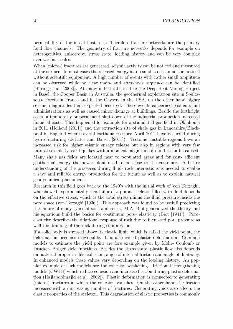
Interactions between fluids and rocks play a crucial role at various natural phe-nomena like volcanic systems, mud volcanoes, earthquake swarms and aftershocksequences. For example experimental observations and an analytical model of the1997 Umbria- Marche seismic sequence show that aftershocks can be triggered byintrusion of fluid pressure in a fault zone. A seal of inpermeable rock separates ahigh pressured,supercritical fluid source, from hydrostatic pressure above the seal.Breaking the seal leads to a propagating pressure pulse along the fault triggeringaftershocks along its way (Miller et al. [2004]). At vulcanic activity the involvmentof fluids is obvious. In 2006 the mud vulcano Lusi in North east Java errupted withmud and gas covering wide ranges (Mazzini et al. [2007]). Again field obersvationsand physical models suggest that through fault slip deeply derived fluids intrudethe fault and mix with an preexisting hydrothermal system feeding the eruption(Lupi et al. [2013]). Also driven by deeply derived fluids are earthquake swarmslike for example in central europe in the Egger rift system (Fischer et al. [2014])or the Matsushiro earthquake swarm in Japan (Cappa et al. [2009]). In both casesoverpressured CO2 arrises from the upwelling mantle, probably connected with mag-matic activity, and intrude into a fault zone where they trigger earthquake swarms.Swarms are characterized by many events with small and middle sized magnitudewithout a main shock.

Due to the increasing demand of fuels in the last decade industrial applicationsutilizing hydrofracturing, which means breaking the rock by injecting high pressuredfluids, brought new impulses into this field of research and opened it to the public.Hydrofracturing for shale gas recovery got a massive boost in the US, pilot projectsof CO2 sequestration started in Europe and geothermal power plants were installedall over the world, to name just some of recent applications. In these stimulationprocesses engineers increase the intrinsic permeability of the host rock by injectinghigh pressure fluid, mostly water or CO2, through one or more boreholes up to adepth of 4 to 5 kilometers. Typical wellhead pressures can be up to 300 bars. Theintrinsic permeability is normally very low, k = 10−16 m2 or less, and the pores arenot well enough connected for a decent fluid flow (Haring et al. [2008]). The highfluid pressure generates (micro-)fractures in the rock and increases permeability. Infractures the permeability can be higher by several magnitudes than the intrinsic

1

2 INTRODUCTION

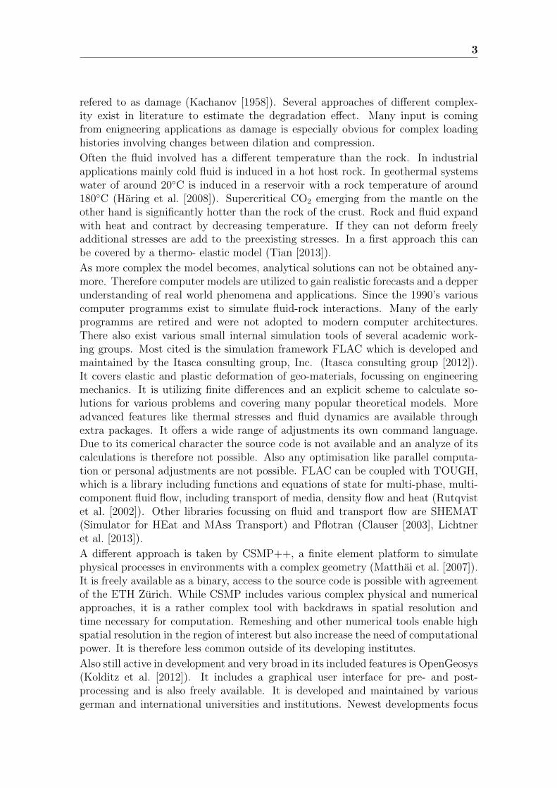
permeability of the intact host rock. Therefore fracture networks are the primaryfluid flow channels. The geometry of fracture networks depends for example onheterogenities, anisotropy, stress state, loading history and can be very complexover various scales.

When (micro-) fractures are generated, seismic activity can be noticed and measuredat the surface. In most cases the released energy is too small so it can not be noticedwithout scientific equipment. A high number of events with rather small amplitudecan be observed while no clear main- and aftershock sequence can be identified(Haring et al. [2008]). At many industrial sites like the Deep Heat Mining Projectin Basel, the Cooper Basin in Australia, the geothermal exploration site in Soultz-sous- Forets in France and in the Geysers in the USA, on the other hand higherseismic magnitudes than expected occurred. These events concerned residents andadministrations as well as caused minor damage at buildings. Beside the forthrightcosts, a temporarly or permenent shut-down of the industrial production increasedfinancial costs. This happened for example for a stimulated gas field in Oklahomain 2011 (Holland [2011]) and the extraction site of shale gas in Lancashire/Black-pool in England where several earthquakes since April 2011 have occurred duringhydro-fracturing (dePater and Baisch [2011]). Tectonic unstable regions have anincreased risk for higher seismic energy release but also in regions with very fewnatural seismicity, earthquakes with a moment magnitude around 4 can be caused.

Many shale gas fields are located near to populated areas and for cost- efficientgeothermal energy the power plant need to be close to the customer. A betterunderstanding of the processes during fluid- rock interactions is needed to enablea save and reliable energy production for the future as well as to explain naturalgeodynamical phenomena.

Research in this field goes back to the 1940’s with the initial work of Von Terzaghi,who showed experimentally that failur of a porous skeleton filled with fluid dependson the effective stress, which is the total stress minus the fluid pressure inside thepore space (von Terzaghi [1936]). This approach was found to be usefull predictingthe failure of many types of soils and rocks. M.A. Biot generalized the theory andhis equations build the basics for continuum poroelasticity (Biot [1941]). Poro-elasticity describes the dilational response of rock due to increased pore pressure aswell the draining of the rock during compression.

If a solid body is stressed above its elastic limit, which is called the yield point, thedeformation becomes irreversible. It is also called plastic deformation. Commonmodels to estimate the yield point are fore example given by Mohr- Coulomb orDrucker- Prager yield functions. Besides the stress state, plastic flow also dependson material properties like cohesion, angle of internal friction and angle of dilatancy.In enhanced models these values vary depending on the loading history. An pop-ular example of such models are the cohesion weakening - frictional strengtheningmodels (CWFS) which reduce cohesion and increase friction during plastic deforma-tion (Hajiabdolmajid et al. [2002]). Plastic deformation is connected to generating(micro-) fractures in which the cohesion vanishes. On the other hand the frictionincreases with an increasing number of fractures. Generating voids also effects theelastic properties of the sceleton. This degradation of elastic properties is commonly

3

refered to as damage (Kachanov [1958]). Several approaches of different complex-ity exist in literature to estimate the degradation effect. Many input is comingfrom enigneering applications as damage is especially obvious for complex loadinghistories involving changes between dilation and compression.

Often the fluid involved has a different temperature than the rock. In industrialapplications mainly cold fluid is induced in a hot host rock. In geothermal systemswater of around 20◦C is induced in a reservoir with a rock temperature of around180◦C (Haring et al. [2008]). Supercritical CO2 emerging from the mantle on theother hand is significantly hotter than the rock of the crust. Rock and fluid expandwith heat and contract by decreasing temperature. If they can not deform freelyadditional stresses are add to the preexisting stresses. In a first approach this canbe covered by a thermo- elastic model (Tian [2013]).

As more complex the model becomes, analytical solutions can not be obtained any-more. Therefore computer models are utilized to gain realistic forecasts and a depperunderstanding of real world phenomena and applications. Since the 1990’s variouscomputer programms exist to simulate fluid-rock interactions. Many of the earlyprogramms are retired and were not adopted to modern computer architectures.There also exist various small internal simulation tools of several academic work-ing groups. Most cited is the simulation framework FLAC which is developed andmaintained by the Itasca consulting group, Inc. (Itasca consulting group [2012]).It covers elastic and plastic deformation of geo-materials, focussing on engineeringmechanics. It is utilizing finite differences and an explicit scheme to calculate so-lutions for various problems and covering many popular theoretical models. Moreadvanced features like thermal stresses and fluid dynamics are available throughextra packages. It offers a wide range of adjustments its own command language.Due to its comerical character the source code is not available and an analyze of itscalculations is therefore not possible. Also any optimisation like parallel computa-tion or personal adjustments are not possible. FLAC can be coupled with TOUGH,which is a library including functions and equations of state for multi-phase, multi-component fluid flow, including transport of media, density flow and heat (Rutqvistet al. [2002]). Other libraries focussing on fluid and transport flow are SHEMAT(Simulator for HEat and MAss Transport) and Pflotran (Clauser [2003], Lichtneret al. [2013]).

A different approach is taken by CSMP++, a finite element platform to simulatephysical processes in environments with a complex geometry (Matthai et al. [2007]).It is freely available as a binary, access to the source code is possible with agreementof the ETH Zurich. While CSMP includes various complex physical and numericalapproaches, it is a rather complex tool with backdraws in spatial resolution andtime necessary for computation. Remeshing and other numerical tools enable highspatial resolution in the region of interest but also increase the need of computationalpower. It is therefore less common outside of its developing institutes.

Also still active in development and very broad in its included features is OpenGeosys(Kolditz et al. [2012]). It includes a graphical user interface for pre- and post-processing and is also freely available. It is developed and maintained by variousgerman and international universities and institutions. Newest developments focus

4 INTRODUCTION

on fluid flow and chemical reactions between rock and fluid but it also containsadvanced mechanical models. Overall it is a feature rich, complex finite- elementprogram, which is also rather demanding in its computational power. The codeSLIM3D is also based on finite elements but utilizes a visco- elasto- plastic rheology(Popov and Sobolev [2008]). This enables the simulator to solve for lithosphericdeformations or plume rising problems as well. On the other hand, it fells short inbrittle mechanics as shear bands can only be generated by introducing initial weakzones.In this thesis I develop a theoretical and numerical model to simulate the defor-mation of rock in response to loading and pore pressure over various scales withan advanced rheological model. One phase as well as multiphase fluid flow is con-sidered, depending on the problem. Also heat transfer can be calculated as well asdeformation and stress it causes. The final model includes therfore thermal, pressureand mechanics (THM- model). The model is capable to calculate dynamic fracturegeneration and fracture growth as well as non-linear behavior in rock and fluid flow.From the numerical side I use a staggered finite difference grid and an explicit timesolution for the dynamics. The simulator is enabled for parallel computing to se-cure short computational times while using a high spatial and temporal resolution.Results are compared to experimental or field observations.This thesis is organized in five chapters. In the first chapter I give a brief introduc-tion in the theoretical and numerical background and a summuray of the scientificarticles. In the second chapter an advanced damage model is introduced which uti-lizes a two- surface approach for the yield- and damage function. Special attentionis paid to the numerical implementation and algorithmic structure. The followingthird chapter introduces a method to determine and locate acoustic emissions in-side a specimen. Hydrofracturing on laboratory scale is considered and numericalresults are compared with experimental data. In the fourth chapter the earthquakeswarm sequences of 2008 along the Eger rift fault plane are simulated by adaptingthe algorithm developed in chapter three to field scale. The last chapter presentsconclusion of this thesis and an outlook towards future research possibilities.This cumulative thesis is organized as a series of papers submitted to internationaljournals. Each one of the chapters two to four is a complete article. As a result ofthis structure, there is some repetition of the physical model and the used methods.The papers included in this thesis are a further development of the basic physicaland numerical model I developed as part of my masters degree at the University ofBonn (Germany) in 2012. The main results of my master thesis are summarized ina scientific article as well and a copy of this submitted scientific paper is providedin the appendix.

1.1. THEORETICAL BACKGROUND 5

1.1 Theoretical Background

The mechanics of rock and soil can be adopted from general solid mechanics. In thissection I present basic theories and equations utilized in further parts of this thesis.The aim of this work is the simulation of rock and fluid behavior. Nevertheless manyof the presented and developed models are not limited to this application.The behavior of material under load is divided into different stages. The linear elas-ticity model based on Hooke’s law is the most simple approach to describe reversibledeformation. For porous media von Terzaghi’s effective stress hypothesis and themodel developed by Biot are the equivalent governing equations. Thermal contrac-tion and expansion can also lead to elastic stresses. Beyond the elastic domain,plastic deformation starts. Based on the perfect plastic model more realistic resultscan be obtained including hardening- softening and damage behavior. Heat andfluid flow are no key aspects of this work but included in the final model. Thereforea short explanation will be provided as well. Further details on the basic rheologicalmodels can be found in Jaeger et al. [2007] and Davis and Selvadurai [2002].

1.1.1 Poro-elasto-plastic Model

1.1.1.1 Poro-elasticity

In solid body mechanics it is more common to use stresses than forces. Stress σ isdefined as force acting over an area. Normal stresses σii perpendicular to the area areseparated from tangential shear stresses σij. In this work stresses are assembled inthe Cauchy stress tensor, which is symmetric. The cartesian coordinate system canbe rotated towards the principal stresses σk with k = 1, 2, 3. In principal directionsshear stresses vanish and only the three principal stresses remain normal to eachother. Due to rotation the trace does not change, therefore

I1 = σ1 + σ2 + σ3 = σxx + σyy + σzz (1.1)

which is the first invariant of the tensor. Using σ′ = σ− 13δijI1, the deviatoric stress

σ′ is defined as the part of the stress which is not connected to volume change.Further invariants of the stress tensor can be defined in cartesian as well as principaldirections,Based on Newton’s second law it can be derived for a two- dimensional solid bodyin x− and y− direction:

∂vx∂t

=1

ρ·(∂σxx∂x

+∂σxy∂y

)∂vy∂t

=1

ρ·(∂σxy∂x

+∂σyy∂y

+ ρg

) (1.2)

where ρ is rock density, v is displacement, g gravitational acceleration and t time.Following the definition of the stress tensor the symmetric infinitesimal strain tensorε is defined with displacement u:

6 INTRODUCTION

εij =1

2·(∂ui(~x, t)

∂xj+∂uj(~x, t)

∂xi

)(1.3)

The relationship between stress and strain is given by Hooke’s law σij = Eijkl · εklwith the elasticity tensor E which depends on the elastic properties, for example thefirst Lame constant λ and shear modulus G. The time derivative of Hooke’s lawgives the governing equations for elastic deformation:

∂σxx∂t

= (λ+ 2G) · ∂vx∂x

+ λ · ∂vy∂y

∂σyy∂t

= (λ+ 2G) · ∂vy∂y

+ λ · ∂vx∂x

∂σxy∂t

= G ·(∂vx∂y

+∂vy∂x

)(1.4)

Von Terzaghi defined effective stresses as (von Terzaghi [1936]):

σtot,ij = σeff,ij + α · pδij (1.5)

where p is pore pressure, the Kronecker Delta and α is the Biot coefficient, whichis usually around 0.8 for porous rock. All derivations above are therefore valid forporous rocks if total stresses are used. Notice that pore pressure only acts alongnormal directions.Considering fluid intrusion in a drained host rock also leads to a change of elasticproperties. Gassmann showed that the bulk module changes with fluid saturationwhile the shear modulus remains constant (Gassmann [1951]). He derived empiricalequations depending on the fluid pressure, porosity and mineral decomposition ofthe rock.Using the Gassmann equation Rice and Cleary expanded the model of Biot using theSkempton coefficient B instead of the Biot coefficient (Biot [1941], Rice and Cleary[1976]):

2 Gεij = σij −ν

1 + νσkkδij +

3(νundr − ν)

B(1 + ν)(1 + νundr)pδij (1.6)

Besides pore pressure pertubations also temperature changes can alter the stressstate. When rock undergoes a temperature change, e.g. because its pore spaceis filled with warmer material, it will change its volume. Thermal strains can becalculated most simple by

εT = −β(T − T0) (1.7)

The thermal strain is negative if the temperature is increased, assuming that thebody expands. The coefficient of thermal expansion β is normally larger than 0 ifthe material expands under heat. We can also define the temperature change

θ = T − T0 (1.8)


If the body is locked and can not deform freely the strains cause stresses. Thesethermal stresses can be derived from the strains but only act in normal directionsand have therefore no shear component. Using the vector I = (1, 1, 0) the stressescan be calculated together with the elastic stresses due to load:

σ = Eεe + βEIθ (1.9)

1.1.1.2 Theory of Plasticity

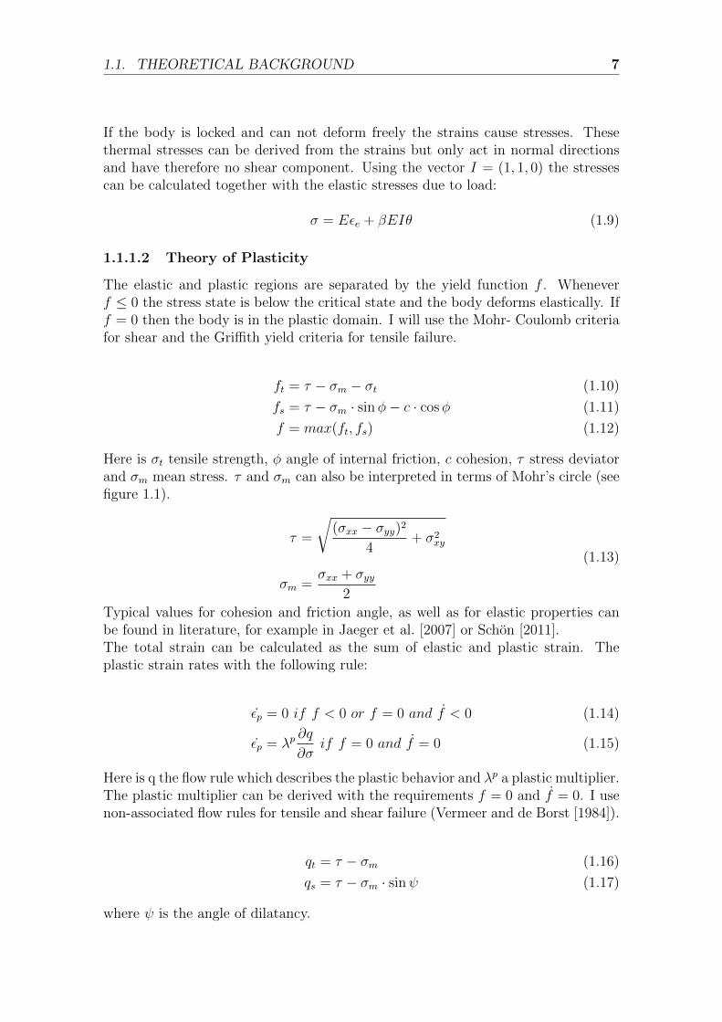
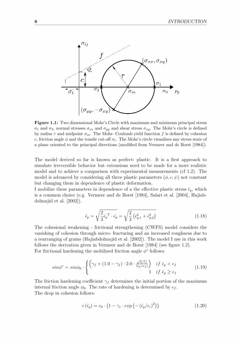
The elastic and plastic regions are separated by the yield function f . Wheneverf ≤ 0 the stress state is below the critical state and the body deforms elastically. Iff = 0 then the body is in the plastic domain. I will use the Mohr- Coulomb criteriafor shear and the Griffith yield criteria for tensile failure.

ft = τ − σm − σt (1.10)

fs = τ − σm · sinφ− c · cosφ (1.11)

f = max(ft, fs) (1.12)

Here is σt tensile strength, φ angle of internal friction, c cohesion, τ stress deviatorand σm mean stress. τ and σm can also be interpreted in terms of Mohr’s circle (seefigure 1.1).

τ =

√(σxx − σyy)2

4+ σ2

xy

σm =σxx + σyy

2

(1.13)

Typical values for cohesion and friction angle, as well as for elastic properties canbe found in literature, for example in Jaeger et al. [2007] or Schon [2011].The total strain can be calculated as the sum of elastic and plastic strain. Theplastic strain rates with the following rule:

εp = 0 if f < 0 or f = 0 and f < 0 (1.14)

εp = λp∂q

∂σif f = 0 and f = 0 (1.15)

Here is q the flow rule which describes the plastic behavior and λp a plastic multiplier.The plastic multiplier can be derived with the requirements f = 0 and f = 0. I usenon-associated flow rules for tensile and shear failure (Vermeer and de Borst [1984]).

qt = τ − σm (1.16)

qs = τ − σm · sinψ (1.17)

where ψ is the angle of dilatancy.

8 INTRODUCTION

Figure 1.1: Two dimensional Mohr’s Circle with maximum and minimum principal stressσ1 and σ3, normal stresses σxx and σyy and shear stress σxy. The Mohr’s circle is definedby radius τ and midpoint σm. The Mohr- Coulomb yield function f is defined by cohesionc, friction angle φ and the tensile cut-off σt. The Mohr’s circle visualizes any stress state ofa plane oriented to the principal directions (modified from Vermeer and de Borst [1984]).

The model derived so far is known as perfect- plastic. It is a first approach tosimulate irreversible behavior but extensions need to be made for a more realisticmodel and to achieve a comparison with experimental measurements (cf 1.2). Themodel is advanced by considering all three plastic parameters (φ, c, ψ) not constantbut changing them in dependence of plastic deformation.I mobilize these parameters in dependence of a the effective plastic stress εp, whichis a common choice (e.g. Vermeer and de Borst [1984], Salari et al. [2004], Hajiab-dolmajid et al. [2002]).

εp =

√2

3εpT · εp =

√2

3

(ε2p,1 + ε2p,2

)(1.18)

The cohesional weakening - frictional strengthening (CWFS) model considers thevanishing of cohesion through micro- fracturing and an increased roughness due toa rearranging of grains (Hajiabdolmajid et al. [2002]). The model I use in this workfollows the derivation given in Vermeer and de Borst [1984] (see figure 1.2).For frictional hardening the mobilized friction angle φ∗ follows:

sinφ∗ = sinφ0 ·

{(γf + (1.0− γf ) · 2.0 ·

√εp·εf

(εp+εf )

)if εp < εf

1 if εp ≥ εf(1.19)

The friction hardening coefficient γf determines the initial portion of the maximuminternal friction angle φ0. The rate of hardening is determined by εf .The drop in cohesion follows:

c (εp) = c0 ·(1− γc · exp

(− (εp/εc)

2)) (1.20)


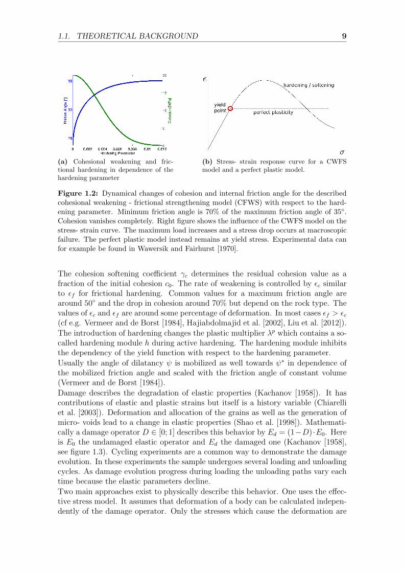
(a) Cohesional weakening and fric-tional hardening in dependence of thehardening parameter

(b) Stress- strain response curve for a CWFSmodel and a perfect plastic model.

Figure 1.2: Dynamical changes of cohesion and internal friction angle for the describedcohesional weakening - frictional strengthening model (CFWS) with respect to the hard-ening parameter. Minimum friction angle is 70% of the maximum friction angle of 35◦.Cohesion vanishes completely. Right figure shows the influence of the CWFS model on thestress- strain curve. The maximum load increases and a stress drop occurs at macroscopicfailure. The perfect plastic model instead remains at yield stress. Experimental data canfor example be found in Wawersik and Fairhurst [1970].

The cohesion softening coefficient γc determines the residual cohesion value as afraction of the initial cohesion c0. The rate of weakening is controlled by εc similarto εf for frictional hardening. Common values for a maximum friction angle arearound 50◦ and the drop in cohesion around 70% but depend on the rock type. Thevalues of εc and εf are around some percentage of deformation. In most cases εf > εc(cf e.g. Vermeer and de Borst [1984], Hajiabdolmajid et al. [2002], Liu et al. [2012]).

The introduction of hardening changes the plastic multiplier λp which contains a so-called hardening module h during active hardening. The hardening module inhibitsthe dependency of the yield function with respect to the hardening parameter.

Usually the angle of dilatancy ψ is mobilized as well towards ψ∗ in dependence ofthe mobilized friction angle and scaled with the friction angle of constant volume(Vermeer and de Borst [1984]).

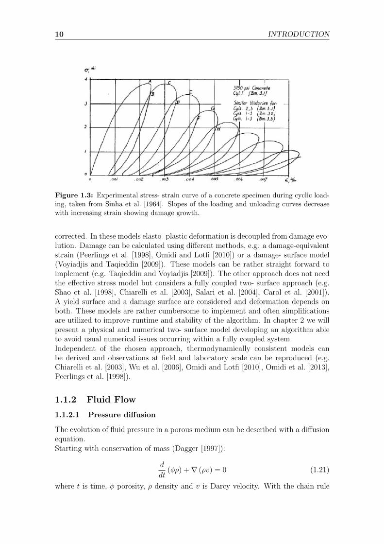
Damage describes the degradation of elastic properties (Kachanov [1958]). It hascontributions of elastic and plastic strains but itself is a history variable (Chiarelliet al. [2003]). Deformation and allocation of the grains as well as the generation ofmicro- voids lead to a change in elastic properties (Shao et al. [1998]). Mathemati-cally a damage operator D ∈ [0; 1] describes this behavior by Ed = (1−D) ·E0. Hereis E0 the undamaged elastic operator and Ed the damaged one (Kachanov [1958],see figure 1.3). Cycling experiments are a common way to demonstrate the damageevolution. In these experiments the sample undergoes several loading and unloadingcycles. As damage evolution progress during loading the unloading paths vary eachtime because the elastic parameters decline.

Two main approaches exist to physically describe this behavior. One uses the effec-tive stress model. It assumes that deformation of a body can be calculated indepen-dently of the damage operator. Only the stresses which cause the deformation are

10 INTRODUCTION

Figure 1.3: Experimental stress- strain curve of a concrete specimen during cyclic load-ing, taken from Sinha et al. [1964]. Slopes of the loading and unloading curves decreasewith increasing strain showing damage growth.

corrected. In these models elasto- plastic deformation is decoupled from damage evo-lution. Damage can be calculated using different methods, e.g. a damage-equivalentstrain (Peerlings et al. [1998], Omidi and Lotfi [2010]) or a damage- surface model(Voyiadjis and Taqieddin [2009]). These models can be rather straight forward toimplement (e.g. Taqieddin and Voyiadjis [2009]). The other approach does not needthe effective stress model but considers a fully coupled two- surface approach (e.g.Shao et al. [1998], Chiarelli et al. [2003], Salari et al. [2004], Carol et al. [2001]).A yield surface and a damage surface are considered and deformation depends onboth. These models are rather cumbersome to implement and often simplificationsare utilized to improve runtime and stability of the algorithm. In chapter 2 we willpresent a physical and numerical two- surface model developing an algorithm ableto avoid usual numerical issues occurring within a fully coupled system.Independent of the chosen approach, thermodynamically consistent models canbe derived and observations at field and laboratory scale can be reproduced (e.g.Chiarelli et al. [2003], Wu et al. [2006], Omidi and Lotfi [2010], Omidi et al. [2013],Peerlings et al. [1998]).

1.1.2 Fluid Flow

1.1.2.1 Pressure diffusion

The evolution of fluid pressure in a porous medium can be described with a diffusionequation.Starting with conservation of mass (Dagger [1997]):

d

dt(φρ) +∇ (ρv) = 0 (1.21)

where t is time, φ porosity, ρ density and v is Darcy velocity. With the chain rule


this equation can be simplified:

1

ρ

∂ρ

∂PP +

1

φρ∇ (ρv) = 0 (1.22)

In porous media different compressibilities have to be considered (Zimmerman [1991]).Besides compressibility of fluid βf also pore space varies with fluid pressure P .

βf = −1

ρ

∂ρ

∂P(1.23)

βφ = −1

φ

∂φ

∂P(1.24)

Darcy’s equation relates fluid flux with pressure gradient for porous media by intro-ducing permeability k and viscosity η

v = −kη∇P (1.25)

If neglecting source and sink terms, the pressure diffusion is given by

∂P

∂t=

1

φ(βf + βφ)∇(k

η∇P

)(1.26)

In geological settings the permeability can vary over a large range. Many authorsconsider it as stress and pressure dependent (e.g. Miller et al. [2004], Carcione andTinivella [2001], Rutqvist et al. [2002], Latham et al. [2013], Bai et al. [1997], Minet al. [2004]). This has also be shown in experimental studies (Blocher et al. [2009]).Different studies (e.g. Miller et al. [2004], Carcione and Tinivella [2001]) use anexponential function of permeability in dependence of the normal stress σn.

k = k0 · exp(−σnσ0

)(1.27)

where k0 is permeability at zero stress, σ0 is a scaling constant and σn can beexpressed with maximal and minimal principal stresses σ1, σ3 and dip angle θ:

σn =σ1 + σ3 − 2P

3+σ1 − σ3

2· cos(2θ) (1.28)

Also some authors chose permeability in dependence of a stress dependent porosity(Rutqvist et al. [2002], Min et al. [2004]):

φ =φr + (φ0 − φr) · exp(a · σn) (1.29)

k =k0 exp[c · (φ/φ0 − 1)] (1.30)

where φ0 and k0 are porosity and permeability at zero stress, φr is a residual value,a and c are constants.Besides pressure and stress dependency, permeability can increase rapidly by severalorders of magnitude if new fractures are generated (Mitchell and Faulkner [2008]).

12 INTRODUCTION

Generally, fractures can have significant higher permeability than intact host rock.For fractures pressure dependency of permeability can even be increased in compar-ison to intact host rock.

1.1.2.2 Two phase flow of water and air

The single phase flow model can be extended considering multiple phases like fluidand gas phase. In the following we will consider a mixture of water and air andassume the phases to be immiscible, isothermal and neglect phase transition. Thesubscripts α = w, a will indicate water and air phase respectively.We will start with the conservation of mass but now considering saturation S ofeach phase (Dagger [1997]):

d

dt(φραSα) +∇ (ραvα) = 0 (1.31)

We perform similar calculations than for the single phase flow, using the definitionsfor compressibilities and the generalized Darcy velocity v. These phase dependentDarcy velocity includes a phase permeability kα which varies between 0 and 1 addi-tionally to the intrinsic permeability k0.

vw = −kw · k0

µw∇Pw (1.32)

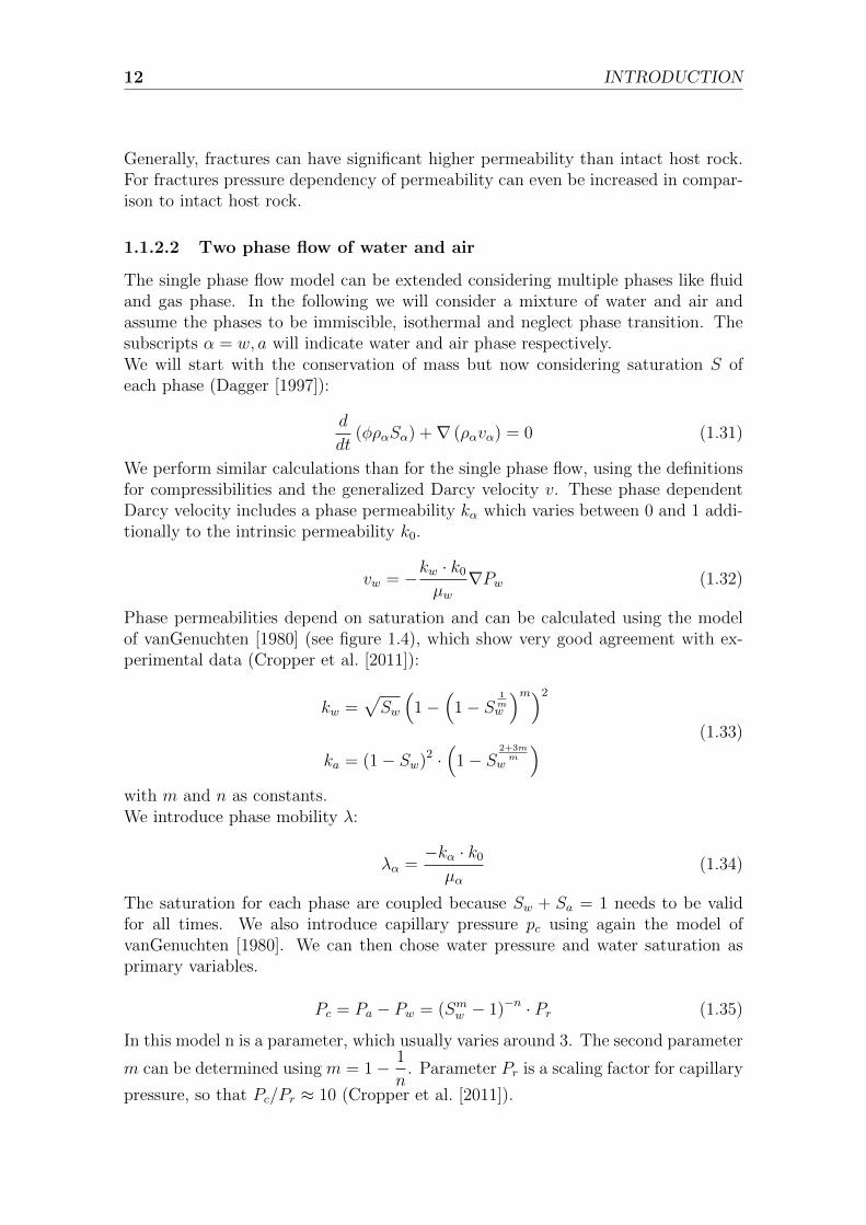
Phase permeabilities depend on saturation and can be calculated using the modelof vanGenuchten [1980] (see figure 1.4), which show very good agreement with ex-perimental data (Cropper et al. [2011]):

kw =√Sw

(1−

(1− S

1mw

)m)2

ka = (1− Sw)2 ·(

1− S2+3mm

w

) (1.33)

with m and n as constants.We introduce phase mobility λ:

λα =−kα · k0

µα(1.34)

The saturation for each phase are coupled because Sw + Sa = 1 needs to be validfor all times. We also introduce capillary pressure pc using again the model ofvanGenuchten [1980]. We can then chose water pressure and water saturation asprimary variables.

Pc = Pa − Pw = (Smw − 1)−n · Pr (1.35)

In this model n is a parameter, which usually varies around 3. The second parameter

m can be determined using m = 1− 1

n. Parameter Pr is a scaling factor for capillary

pressure, so that Pc/Pr ≈ 10 (Cropper et al. [2011]).


Figure 1.4: Phase permeability calculated with the model of vanGenuchten [1980] independence of the water saturation. For a drained case water permeability is zero andincreases with increasing saturation towards the intrinsic permeability. Permeability of airphase decreases simultaneously.

Two strongly coupled, parabolic differential equations exist for the two primaryvariables Sw, Pw, which is called the Pressure- Saturation formulation. It is notlimited to homogeneous systems and converges towards one phase flow for saturationclose to 1 (Helmig [1997]).

∇ (λw∇Pw) = φ

(Swcw

∂Pw∂t

+∂Sw∂t

)

∇ (λa∇ (Pc + Pw)) = φ

((1− Sw) ca

∂ (Pc + Pw)

∂t− ∂Sw

∂t

) (1.36)

To decouple the equations we assume the air to be infinitely mobile, which meansthe air reservoir is infinitely large and air can moves freely. The air pressure isunder this assumptions constant over the whole domain and can be chosen as thezero reference (Richards [1931]). The capillary pressure becomes Pc = −Pw and theRichards equation remains.

∂Pw∂t

=1

φ (Sw · cw + C (Pw))∇ (λw∇Pw) (1.37)

with capacity C (Pw) = ∂Sw∂Pw

, which is defined by equation 1.35.

1.1.2.3 Heat Transport

The fundamentals of heat transport in a porous media are described by the conser-vation of energy. I use a so called non-local approach in which I calculate fluid- and

14 INTRODUCTION

rock temperature separately. Heat is exchanged over the contact surface depend-ing on the material properties. Several values here have to be estimated as theyare difficult to determine in laboratory and almost impossible to estimate on fieldscale. Especially contact area A and overall hear transfer coefficient h suffer fromthis inaccuracy and have to be estimated for highly fractured reservoirs (Shaik et al.[2011]).We determine heat transfer Q as:

Q = hA (Tf − Tr) (1.38)

where T is temperature of fluid f and rock r. This transfer term is equal to thesource or sink term in the conservation of energy. Note that different signs for thetransferred heat need to be used between fluid and rock respectively. Heat transportin the solid is described by a diffusion equation.

∂Tr∂t

=κr

(1− φ)ρrcpr∇2Tr +

1

(1− φ)ρrcprQ (1.39)

where φ is porosity, κr thermal conductivity, ρ density and cpr heat capacity (Bejan[2013]). The heat of the fluid is limited to the pore space but also considers anadvection term with Darcy velocity v.

∂Tf∂t

=κf

φρfcpf∇2Tf −

1

φρfcpfQ−∇(vTf ) (1.40)

This model is limited to a saturated environment and neglects phase changes whichcould occur if temperature exceeds given limits for the materials. We also considernon additional heat sinks or sources. This could easily be done by adding extraterms but is out of scope for the use case in this work.

1.1.3 Numerical Implementation

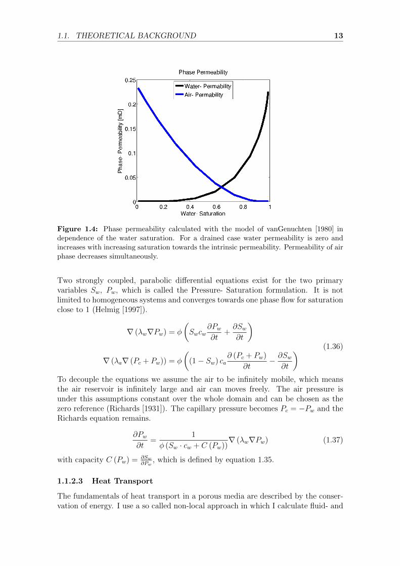
The resulting set of equations of the derived theoretical model is way to complex tobe solved analytically. Therefore numerical simulations are used to obtain resultsfor specific cases and scenarios. In this section I will shortly explain the numericalscheme used for this work.I use finite differences with a staggered grid described in Saenger et al. [2000] andCruz- Atienza and Virieux [2004] as well as explicit time stepping (Virieux [1986]).Simplified, this staggered grid can be thought as three grids, each one shifted halfa grid step in reference to the other (see figure 1.5). The sizes of the grid are onepoint less in each dimension in comparison to the further one. The largest grid isused to calculate the total stresses. Besides the total stresses also fluid pressure andtemperature are defined on these grid points. The next one is the velocity grid. Sovelocity and displacement are defined on this grid. The smallest grid is identicalwith the outermost total stress grid but has two grid points less in each dimension.It is the effective stress grid. On this grid the effective stresses are defined but alsomost of the other variables like yield function, hardening parameter etc.


Figure 1.5: Symbolic sketch of the used staggered grid. Three grids are used and shiftedto each other by half the grid site. Blue dots for the outermost total stress grid, yellowboxes for the velocity grid and green triangles for the effective stress grid. Each grid isone grid point less in each direction than the next one. Boundary conditions only need tobe applied in the total stress grid. See also Saenger et al. [2000].

The used staggered grid has several advantages. First of all the structure of thestaggered grids enables a straightforward building of the differentials. The differen-tials are build symmetrically in all directions. The number of involved grid pointsfor each differential depends on the chosen order of the Taylor approximation inthe finite difference derivation. I use second and fourth order (Cruz- Atienza andVirieux [2004]). The discretized formulation of the equations can be found in Virieux[1986] and Rozhko [2007]. Also the chosen grid only needs boundary conditions forthe variables defined on the outermost grid. These can be overwritten, if needed,by additional boundary conditions for the velocity. This is for example useful if ano-slip boundary is applied.

The staggered grid is very suitable for parallelization with distributed memory. Sev-eral developed algorithms presented in this work need high computational powerand a small spatial and temporal resolution. Both increase the runtime of the sim-ulation. Therefore the load is distributed over several cores and nodes. Most simu-lations were performed using the KRYPTON cluster of the Geodynamics Group ofthe Steinmann Institute, University of Bonn. This cluster consists of 8 nodes with6 cores each. I achieved the best results, meaning shortest runtime of a simulation,using a hybrid parallelization. Parallelization techniques can roughly be separatedin shared and distributed memory. In a shared memory environment all involvedCPU (central processing unit) cores access the same physical memory but each coreonly executes its own spatial domain. I use openMP as a command tool for sharedmemory parallelization. The advantage hereby is that the spatial decomposition isdown by openMP itself, depending on the capacity and workload of the availablecores. The disadvantage of this method is the need for common physical memorywhich means for the KRYPTON cluster that openMP can only be used inside ofeach node distributing over the six available cores.

To communicate between separated nodes with distributed memory I use openMPI.

16 INTRODUCTION

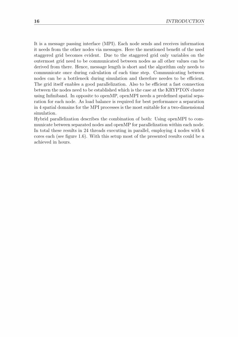
It is a message passing interface (MPI). Each node sends and receives informationit needs from the other nodes via messages. Here the mentioned benefit of the usedstaggered grid becomes evident. Due to the staggered grid only variables on theoutermost grid need to be communicated between nodes as all other values can bederived from there. Hence, message length is short and the algorithm only needs tocommunicate once during calculation of each time step. Communicating betweennodes can be a bottleneck during simulation and therefore needes to be efficient.The grid itself enables a good parallelization. Also to be efficient a fast connectionbetween the nodes need to be established which is the case at the KRYPTON clusterusing Infiniband. In opposite to openMP, openMPI needs a predefined spatial sepa-ration for each node. As load balance is required for best performance a separationin 4 spatial domains for the MPI processes is the most suitable for a two-dimensionalsimulation.Hybrid parallelization describes the combination of both: Using openMPI to com-municate between separated nodes and openMP for parallelization within each node.In total these results in 24 threads executing in parallel, employing 4 nodes with 6cores each (see figure 1.6). With this setup most of the presented results could be aachieved in hours.


Figure 1.6: The simulated spatial region is divided into 4 domains. Each domain ishandled by one MPI- process per node. Within each MPI process the load is shared by 6openMP (OMP) threads, one for each core. In total 24 threads are executing in parallel.Each MPI process only needs to communicate with its two direct neighbors to minimizecommunication.

18 INTRODUCTION

1.2 Summary of scientific articles

In this section I present a short summary of the scientific papers which are part ofthis work

1.2.1 Return algorithm for a strongly coupled elasto-plasticdamage model for rock and concrete

This paper focus on the numerical implementation of a two surface elastoplasticdamage model. In numerical damage mechanics so called effective stress models arecommon. In these models it is assumed that deformation in a material is independentof the damage state and only stresses depend on the damage operator. The equationsare therefore less coupled and can be implemented in almost any elasto- plasticmodel. In the fully coupled model as derived in part I with a yield and a damagefunction this is more complex.

We use a classic elastic predictor - plastic corrector scheme as a starting point,separating elastic and plastic deformation. In every time step we test the damagefunction twice: once after the elastic and again after the plastic deformation. Ifdamage evolves we correct the elastic stresses and recalculate the plastic stressesfollowing the equations derived in part I of these consecutive papers.

This paper also pays attention to a numerical issue which arises whenever functionsfollowing the Kuhn- Tucker conditions are used. The damage and the yield functionare only defined on the negative half space including zero. Due to floating pointarithmetic the zero can not be exactly calculated which leads to a so called ’surfacedrift’. These drift occurs in every time step and is additive. Therefore it needs to beprevented. In plastic calculations several algorithms exist handling these problems.We show that it is critical to consider such a drift from the damage surface as welland develop algorithms for a two surface model analog to a yield surface drift. Tovalidate our approach we compare simulation results with experimental data as wellas with numerical studies of other authors.

1.2.2 A new method to estimate the occurrence and mag-nitude of simulated rock failure events

In material sciences acoustic emissions are a popular tool to test and observe a solidbody. They occur in various materials (metal, ceramic, polymer, concrete, rock) andsignal the development a new fracture or the growth of an existing one. In geoscienceacoustic emissions have the same source mechanism than seismic wave. They areoften used as an analog for seismic waves on laboratory scale. In continuum mechanicthere is no dedicated value which describes an acoustic emission. As they are wavesthe velocity and displacement are natural parameters for the wave but in numericalgeotechnical simulations time steps are much larger than the wave frequency andso the waves itself are not captured. This would also be numerically inefficient.There exist other approaches linking acoustic emissions to the yield function, the

1.2. SUMMARY OF SCIENTIFIC ARTICLES 19

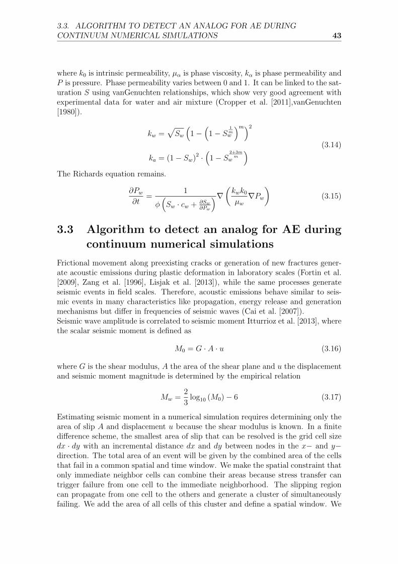
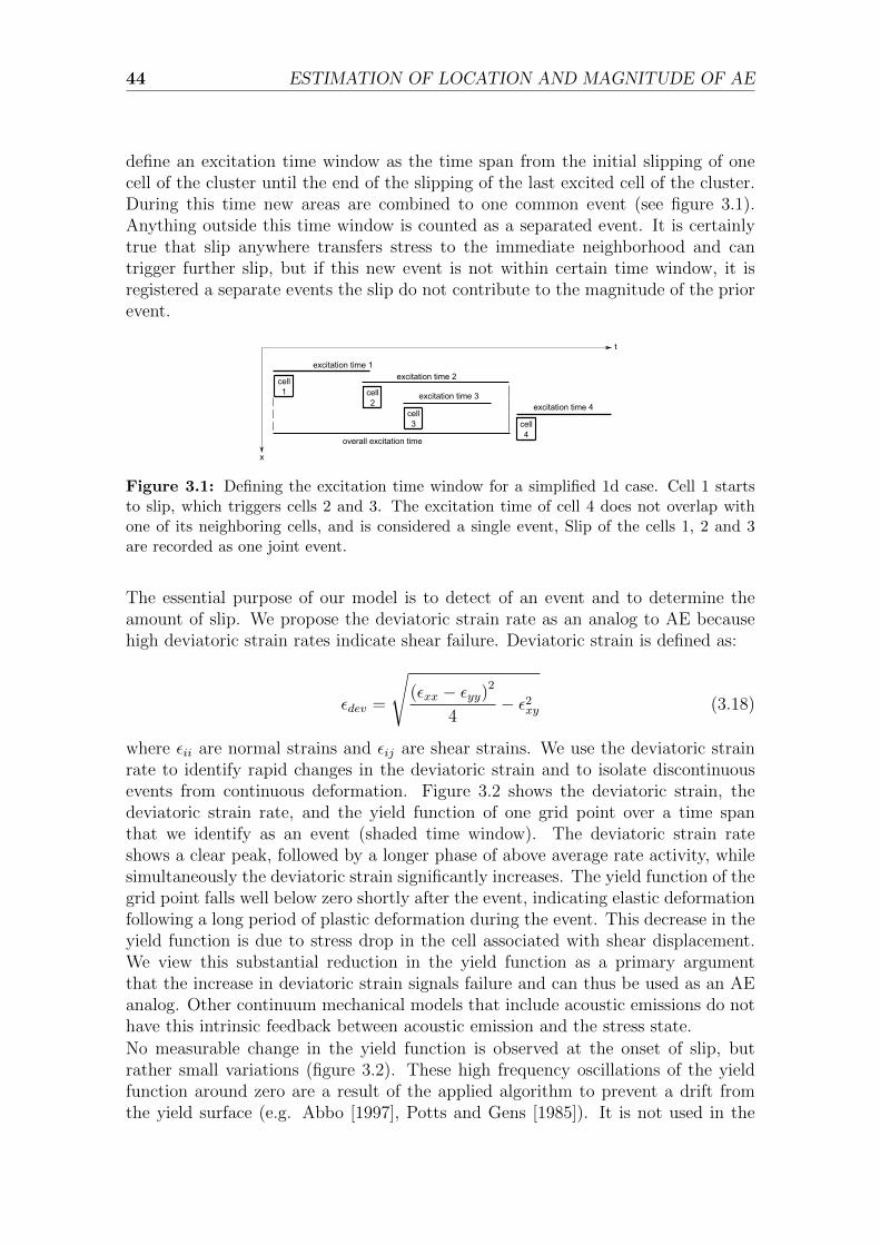
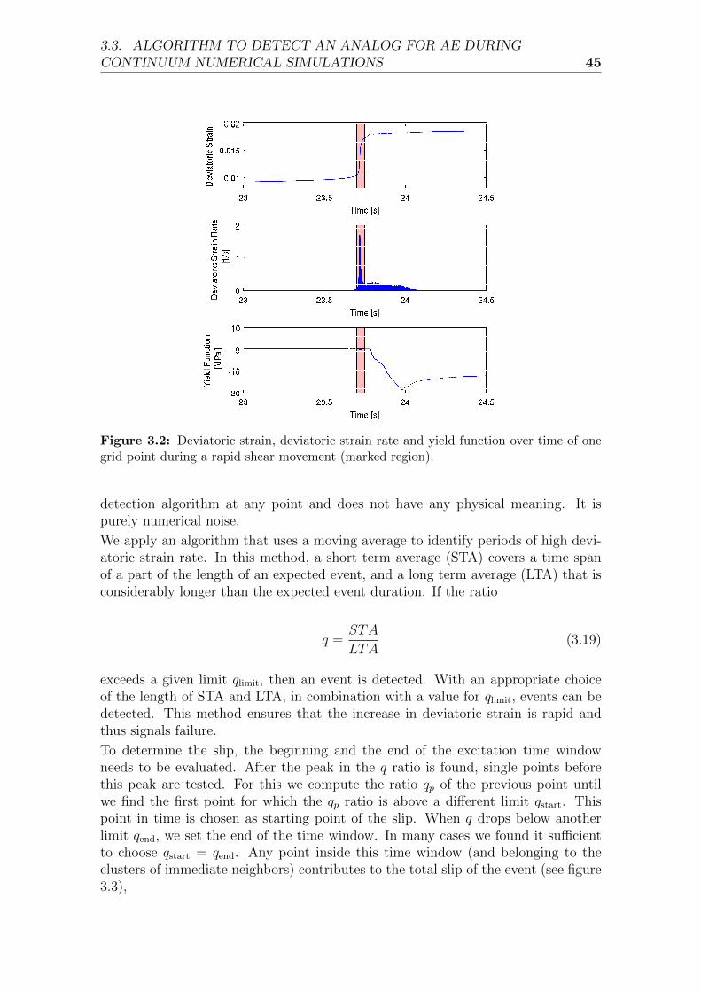
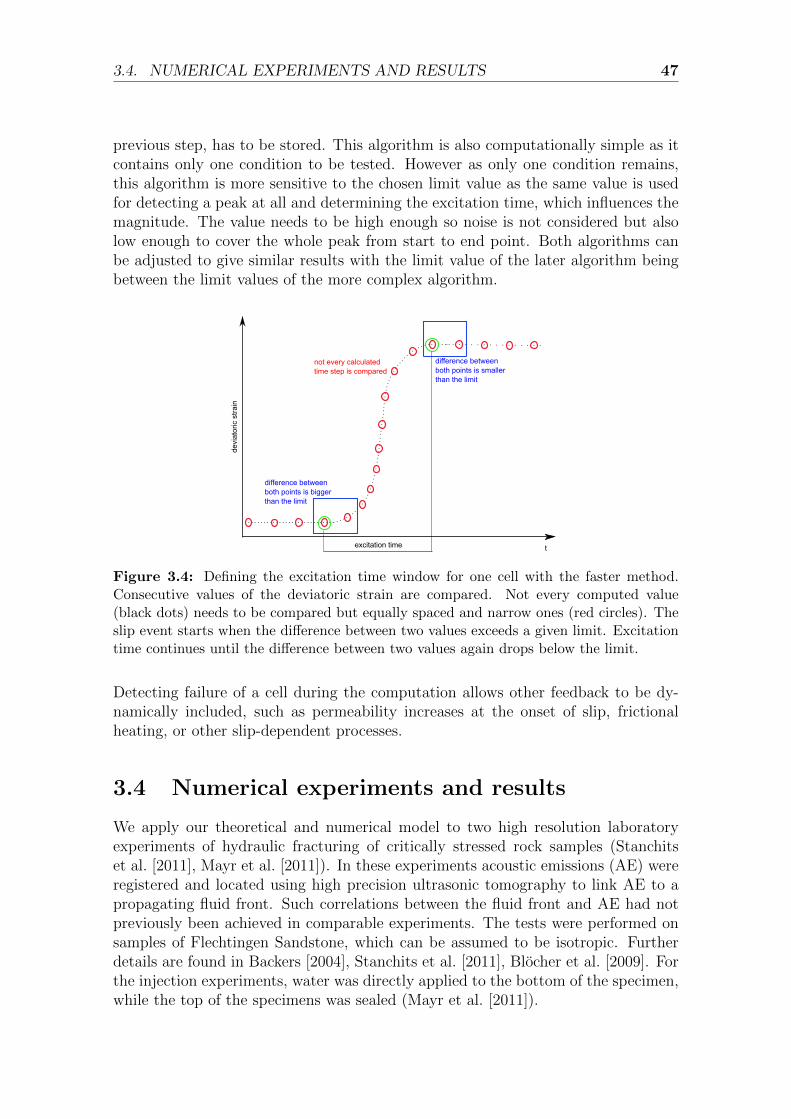
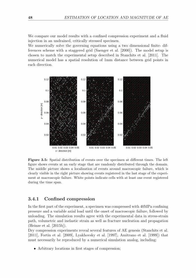
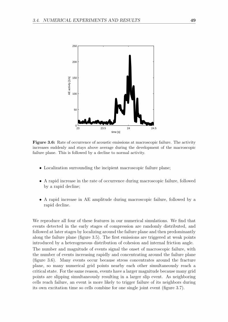
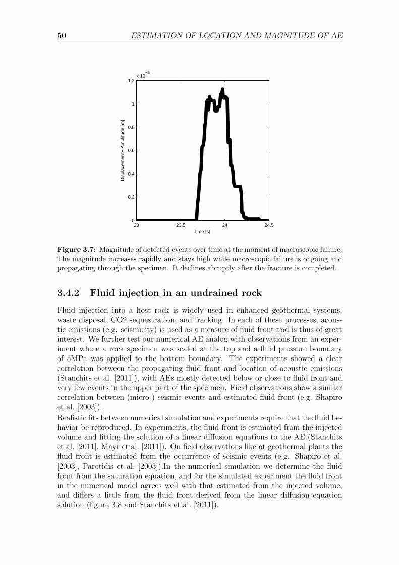
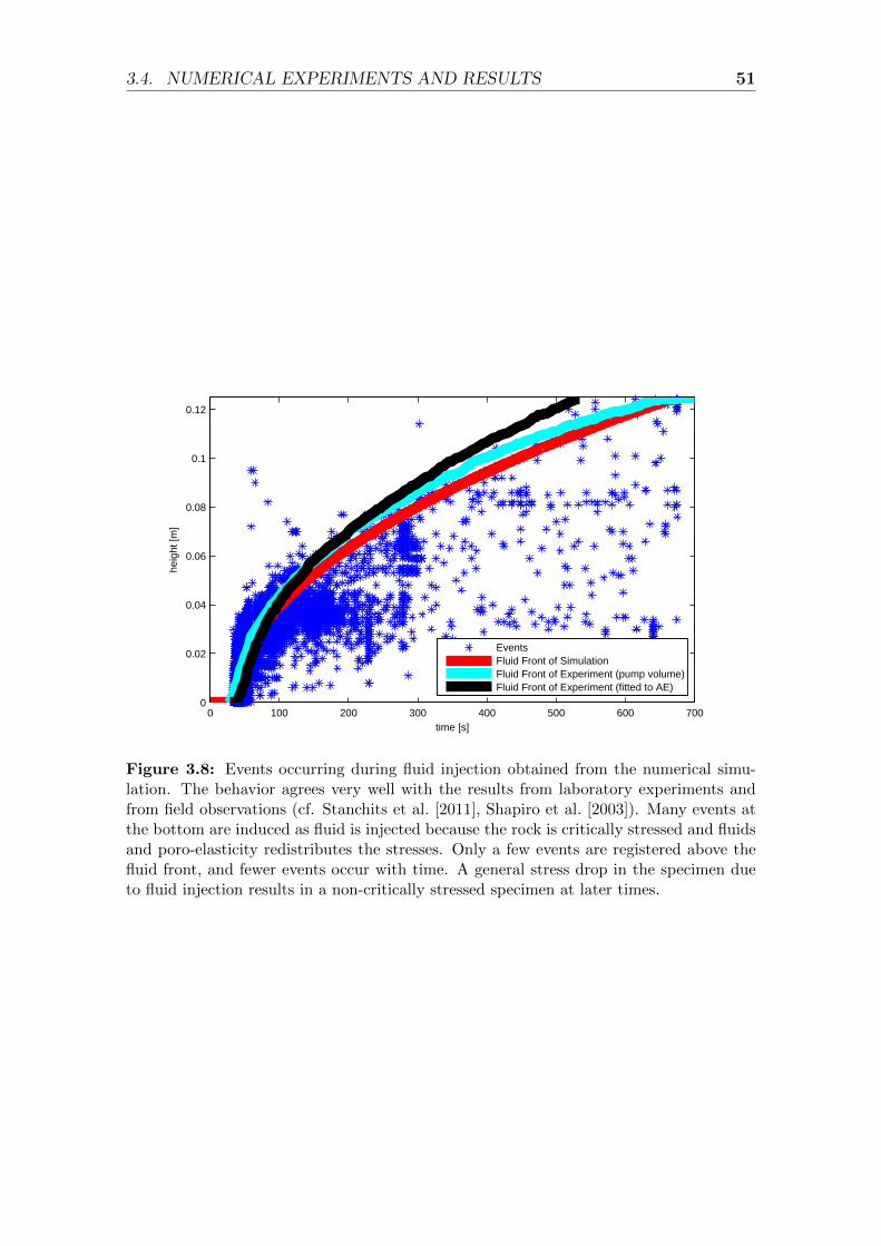
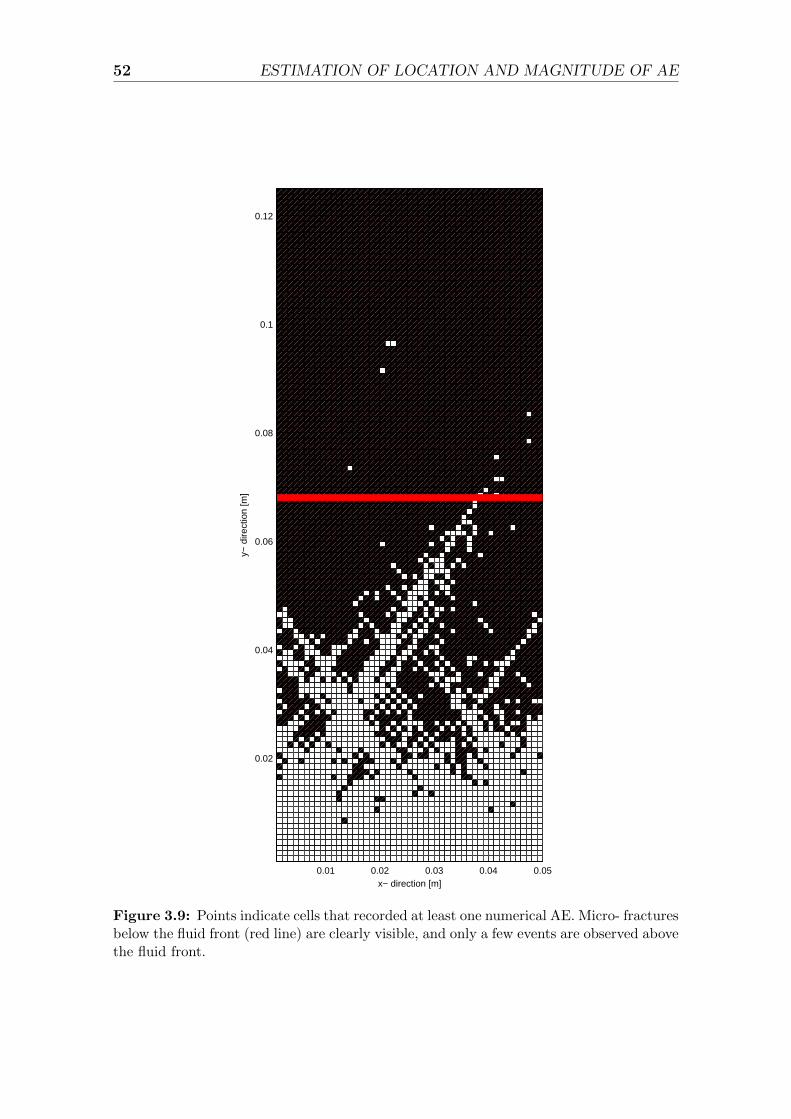
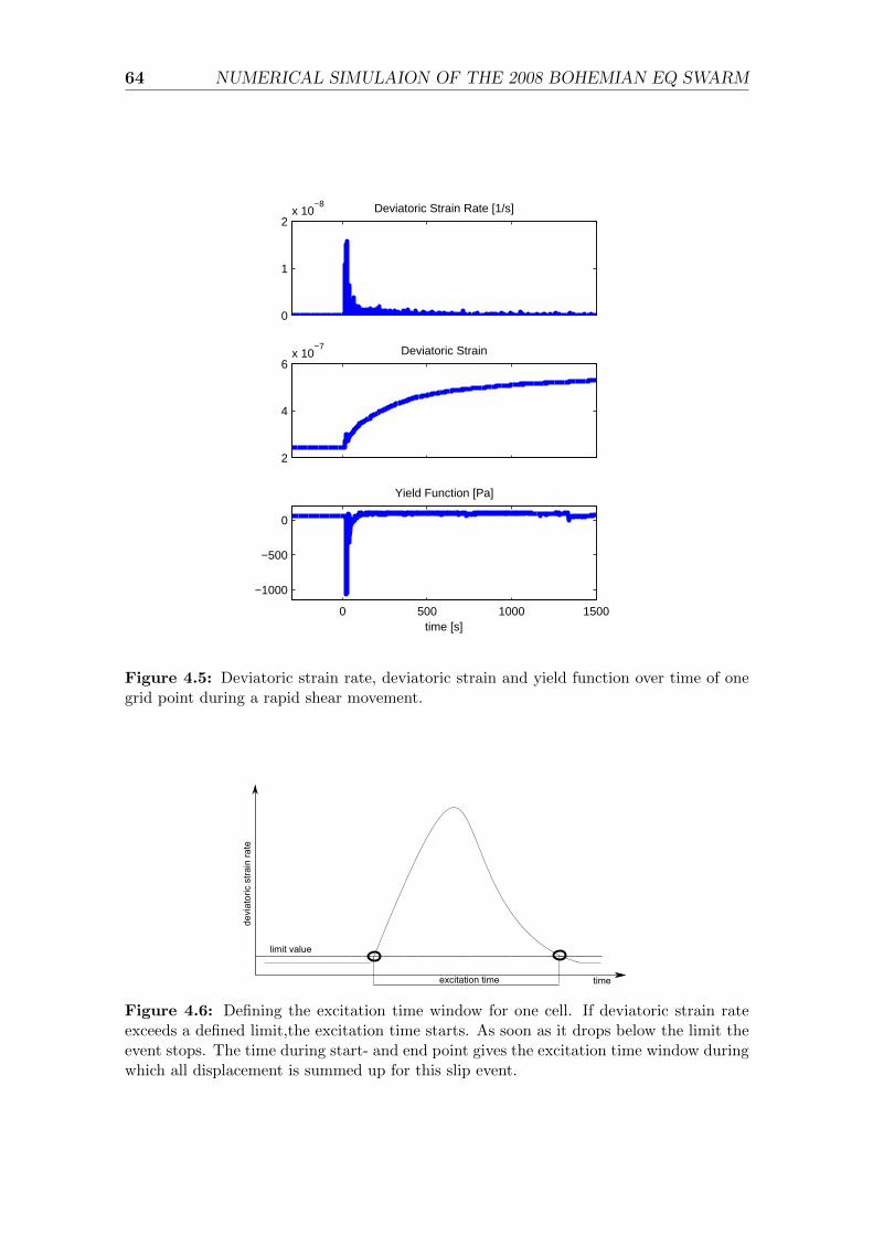
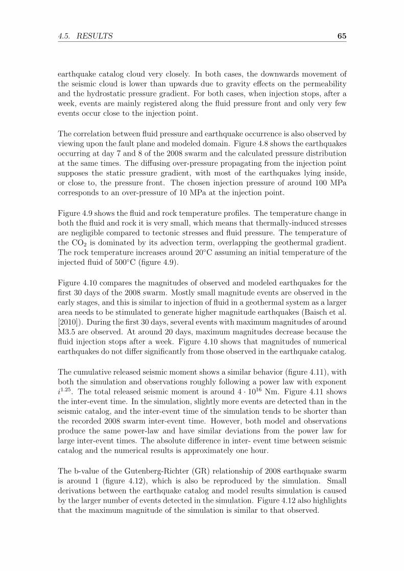
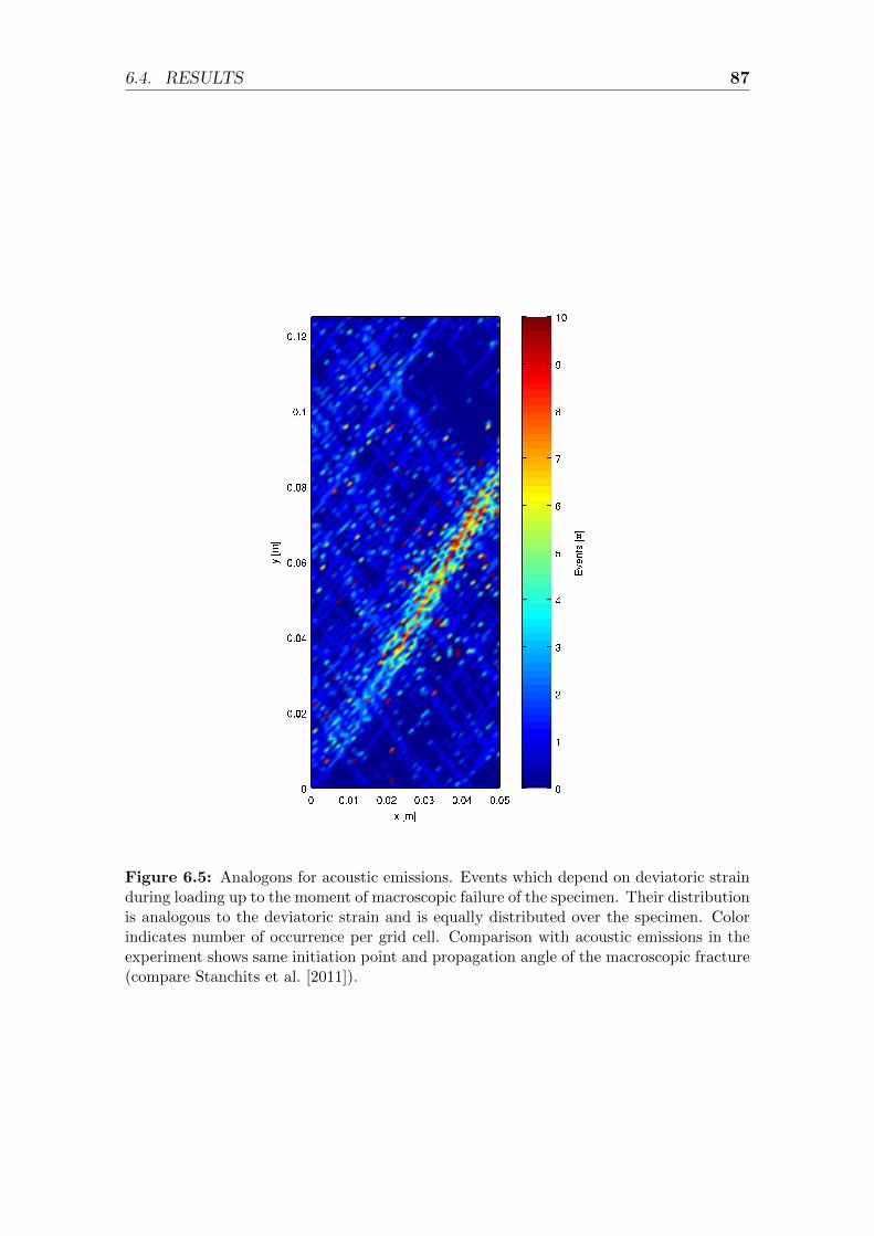
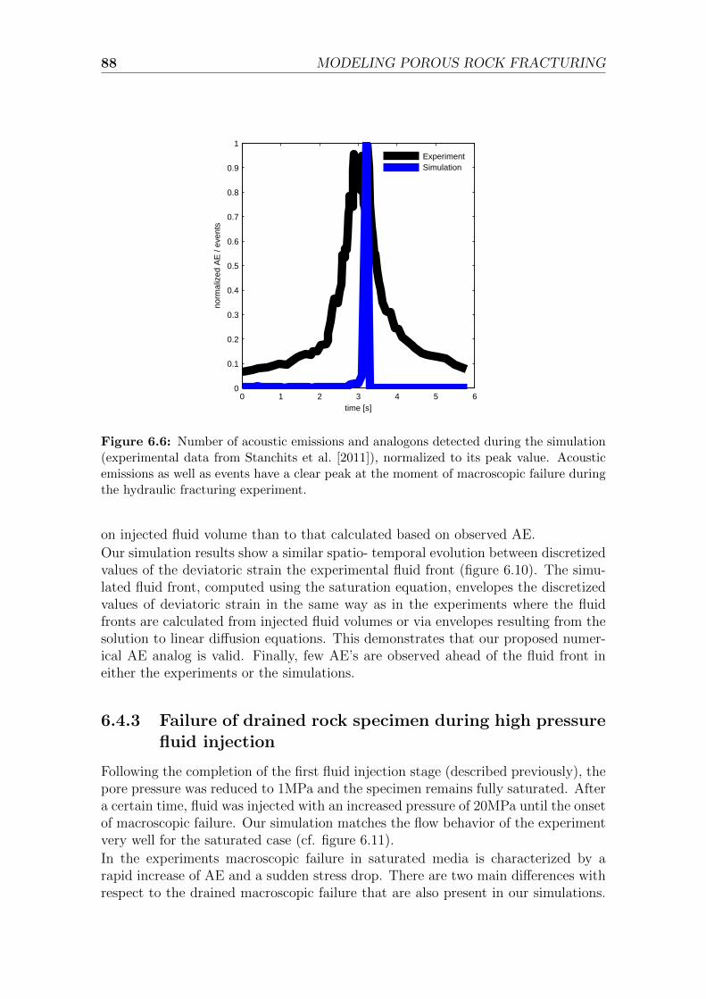
damage parameter or other defined properties which all have different advantagesand disadvantages.We propose the deviatoric strain rate as a proxy for acoustic emissions in numericalsimulations. The deviatoric strain is the part of the strain which is connected toshear movement. Rapid changes in deviatoric strain can be observed at fracturegeneration and propagation. This leads to a rapid increase in deviatoric strain andis followed by a drop in the yield function due to stress release after the slip. In thispaper we present two algorithms to detect rapid changes in the yield function. Onealgorithm uses the ratio of short- and long- term moving average of the deviatoricstrain rate, the other uses the slope of the deviatoric strain to detect events. Withthese methods we are able to calculate the seismic moment using the area of slipand the displacement of the event. A method to determine the area of slip andthe displacement is given. The seismic moment can be compared with the waveamplitude of an acoustic emission.We identify several important features of acoustic emissions which occur duringvarious experiments. We test our approach by implementing the developed algorithmin a numerical model and simulate several laboratory experiments in drained andundrained conditions. We achieve a very well agreement between the events detectedduring numerical simulation and the laboratory results.

1.2.3 Numerical Simulation of the 2008 Bohemian earth-quake swarm

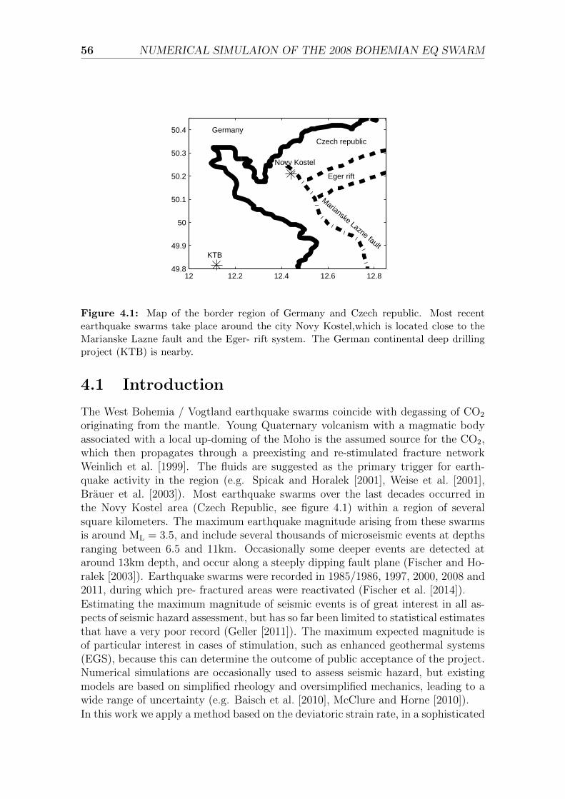
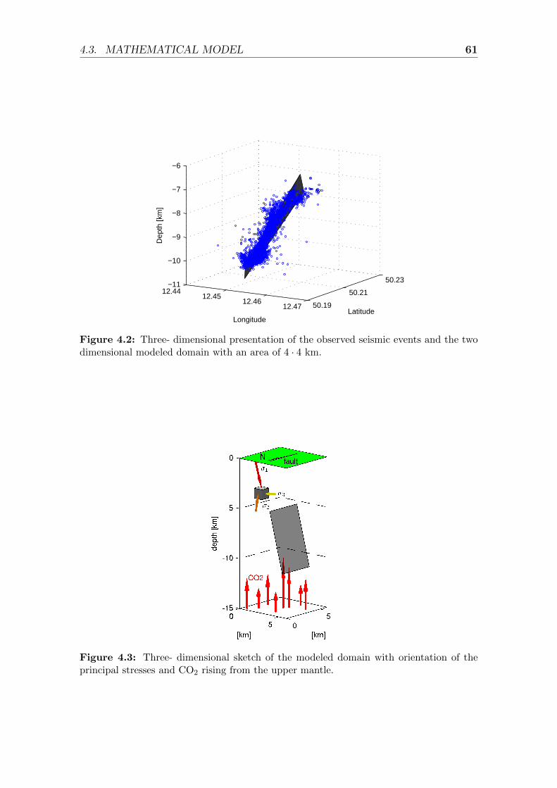
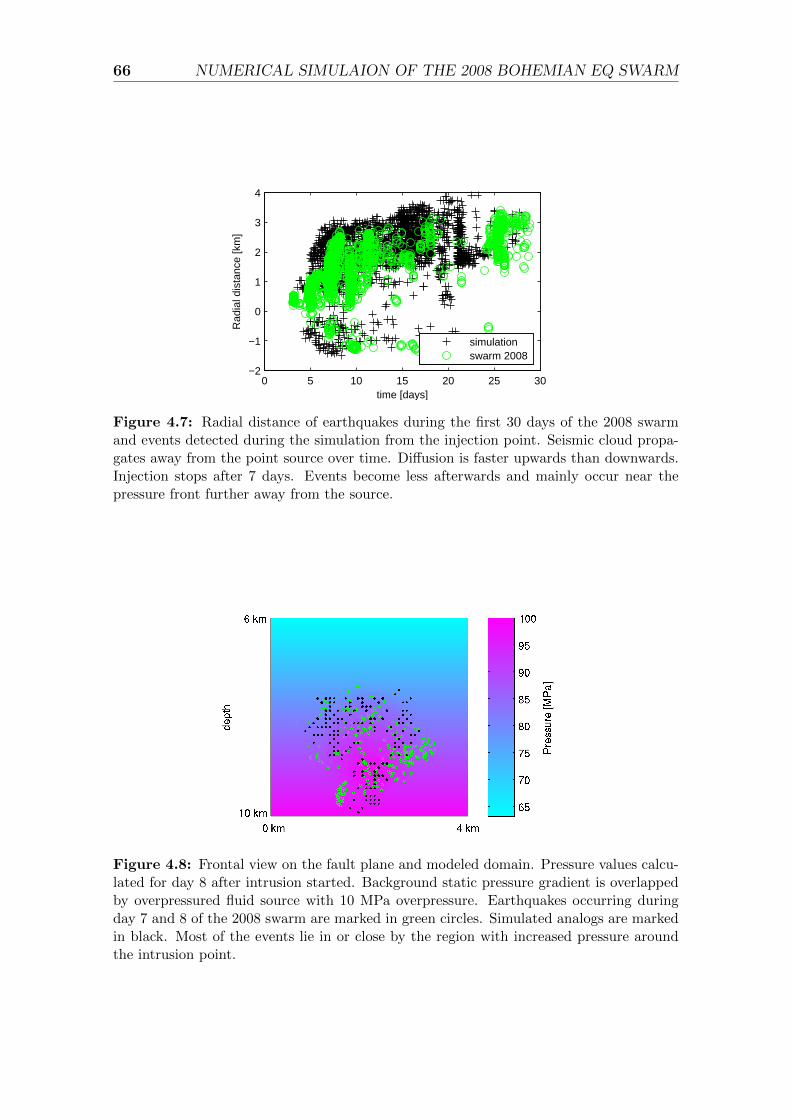
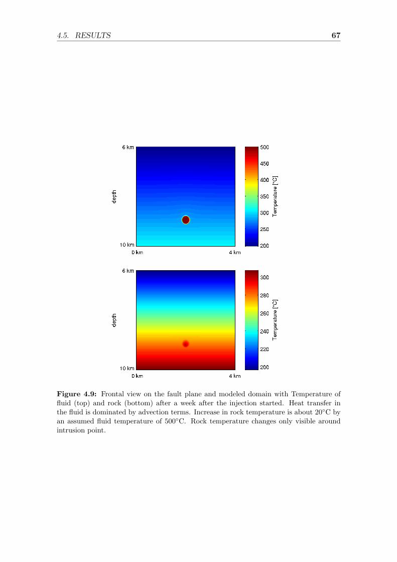
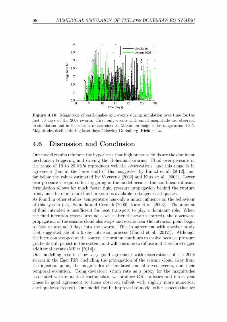
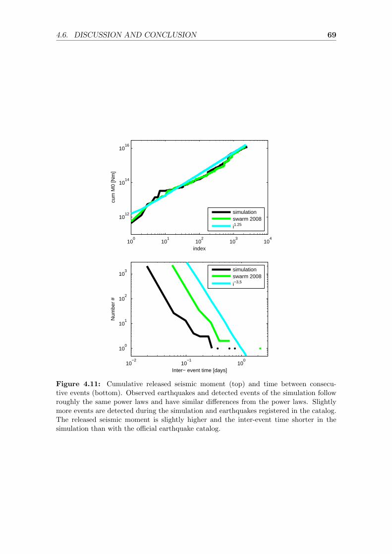
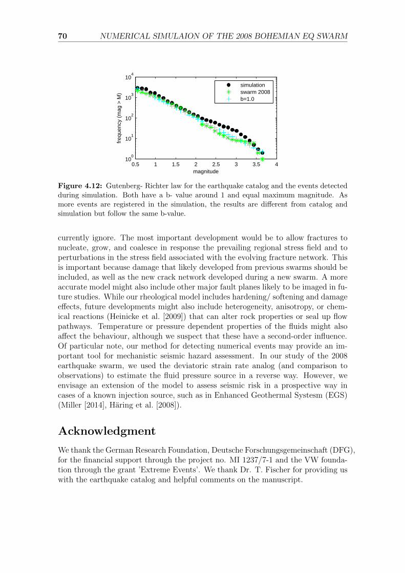
Earthquake swarms occur in the Eger Graben system since centuries. In the lastdecades swarms mainly concentrate around the city Novy Kostel in the german -czech border region. Many mofettes and springs with high CO2 concentration aswell as the mineral decomposition of the gases indicate that swarms are driven byoverpressured, supercritical CO2 emerging from the upper mantle. I simulate theregion using the developed THM model outlined before to simulate the 2008 swarmoccurring on the southern subcluster of the fault system. I use the algorithm todetect acoustic emission in rock specimens, presented in the scientific paper before,to detect and localize earthquakes in the numerical simulation and determine theirmagnitude.With these tools I am able to reproduce the seismic characteristics of the regionin general and of the 2008 swarm like the Gutenberg- Richter law, the magnitudechange over time as well as the spatial- temporal evolution of the earthquakes. Ishow that a point source with a pressure of around 10 - 20 MPa above hydrostaticis sufficient to initiate the swarm while thermal effects can be neglected. Also theunequal evolution of earthquakes below and above the source can be reproduced dueto the hydrostatic pressure and gravity effects on the permeability. I also show thatthe adopted algorithm to look for analogs for earthquakes in a numerical simulationis able to reproduce all characteristic patterns of the earthquakes within the modeledregion.

20 RETURN ALGORITHM COUPLED ELASTO PLASTIC DAMAGE MODEL

Chapter 2

Return algorithm for a stronglycoupled elasto-plastic damagemodel for rock and concrete

Abstract

In this article we present a numerical algorithm for the computation of a strongly-coupled formulation of the poroelasto- plastic damage model including hardeningand softening. We use a yield surface as well as a damage surface to calculateplastic deformation and damage growth. Implementation of such a fully coupledtwo- surface plastic damage model can be cumbersome. The algorithm we presentin this work considers four possible cases: purely elastic deformation, elastic damage,purely plastic deformation and plastic damage. We use an elastic predictor- plasticcorrector scheme as a base and divide any predictor step in an elastic and a plasticcontribution towards deformation and damage growth. Elastic and plastic damagecontributions are then tested separately with the damage surface. While normally intwo-surface plastic damage models drift from yield- and damage surfaces is neglected,we show that these drifts are significant and need to be prevented using returnalgorithms. Our algorithm is based on thermodynamic conjugated forces payingspecial attention to the damage surface drift.Our model is implemented into a finitedifference staggered grid. Functionality ofmodel and algorithm is validated through several tests and comparisons with ex-perimental data available in literature. The simulated results show good agreementwith experimental data and prevention of numerical surface drift.


2.1 Introduction

There are two different approaches to model damage effects: effective plasticity plusdamage and the coupled plasticdamage models. In the first models the plasticity iscalculated in the effective stress space, while continuum damage mechanics is usedto determine stiffness degradation. This method decouples stiffness degradation andplastic deformation and is therefore straightforward to implement in any workingelasto- plastic model. Here the effective stress principle is used which assumes thatdamaged and undamaged rock deform the same way. Deformation is calculated us-ing the undamaged stresses and elastic parameters. These stress values are correctedusing the damage operator but the corrected stresses are not used in the next timestep to calculate the deformation and the elastic properties are kept constant dur-ing the whole deformation. The damage operator is calculated following differentapproaches, even two- surface models with decoupled yield and damage function arepossible. With the damage operator the stresses are corrected. Thermodynamicallyconsistent models can be derived, (e.g. Voyiadjis and Taqieddin [2009], Wu et al.[2006], Grassl and Jirasek [2006], Bobinski and Tejchman [2006], Marzec and Tejch-man [2012], Omidi et al. [2013], Mortazavi and Molladavoodi [2012]). Numericalimplementation is described in detail in (e.g. Taqieddin and Voyiadjis [2009], Shaoet al. [2006], Bielski et al. [2006], Omidi and Lotfi [2010], Xie et al. [2011]).

On the other hand, combined plasticdamage models result in strongly coupledequations by using the degradation of elastic properties for calculating deformation(e.g. Shao et al. [2006], Salari et al. [2004], Chiarelli et al. [2003]). Then, thesemodels can be calibrated directly using experimental observations. We see the mainadvantage of these coupled models by avoiding the assumption of effective stresses.While the use of effective stresses is a widely accepted assumption, it rest on con-sidering plastic deformation completely decoupled to damage evolution, which isunreal. However, it is generally preferred over the coupled plastic damage modelsbecause coupled models results in complex algorithms which often become unstable(Taqieddin [2008]).

As plasticdamage models result in a complicated numerical scheme, their numeri-cal implementation is often simplified when it comes to numerical yield surface drift(Potts and Gens [1985], Sloan [1987]). This drift occurs in any numerical simulationusing continuum elasto- plastic equations independent of the numerical grid, chosenmethod or yield function. It describes the fact, that calculated values for the yieldsurface during plastic deformation will always differ slightly from zero. These dif-ferences add up in every time step and influence the results dominantly if no returnalgorithm is used to prevent and limit further drift. Several stable algorithms existto prevent surface drift with any arbitrary accuracy. An overview about methodsand implementation can be found in Potts and Gens [1985] and Abbo [1997].

In coupled plasticdamage models, a double surface approch is used (Carol et al.[2001]), one surface associated to yielding and the other one related to damageevolution from which drifting is also possible. We present an explicit numericalalgorithm for a double surface model, considering numerical drift from both surfaces.We follow the evolution of damage, its drifting from the damage surface and its

2.2. RHEOLOGICAL MODEL 23

influence on the stresses. Our model is verified with comparison to experimentaldata.In the following section we will derive our rheological model and proceed by present-ing the developed overall algorithm considering all possible combinations: purelyelastic, elastic damage, purely plastic and plastic damage and describe in detail thesurface drift algorithm for the coupled plasticdamage case. In the fourth sectionthe model is tested by simulating various scenarios and experiments. The work isconcluded with a discussion of model and algorithm.

2.2 Rheological Model

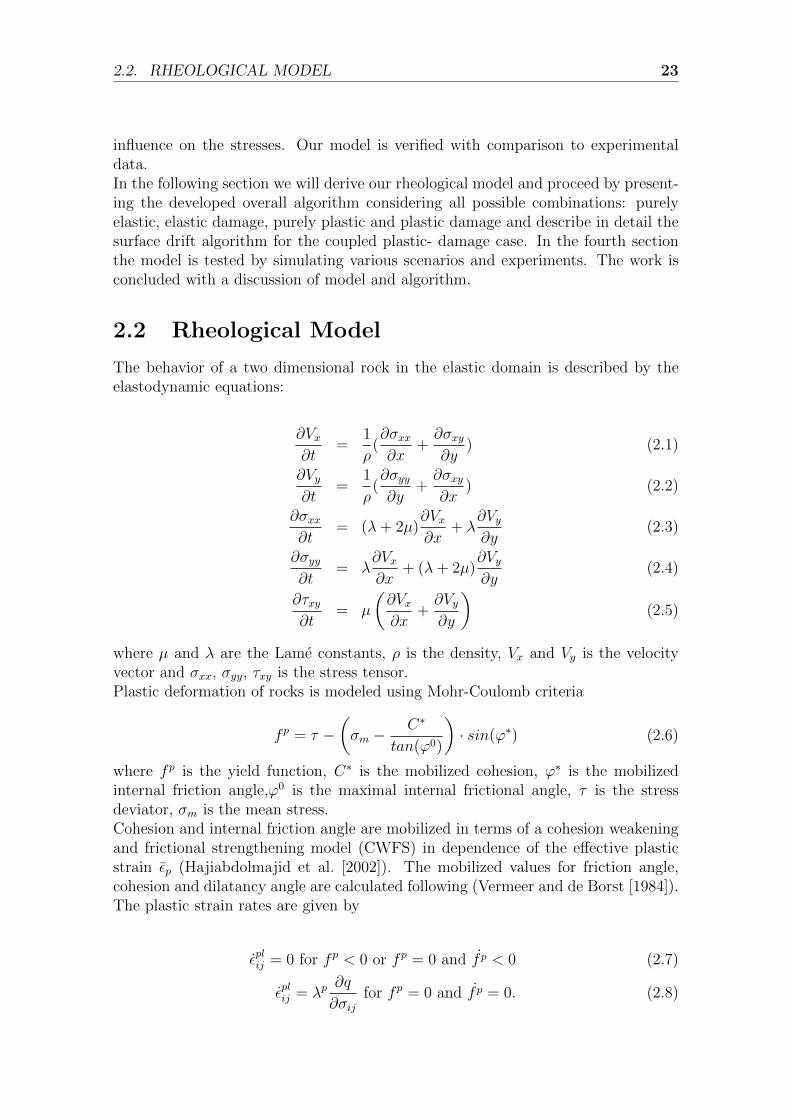
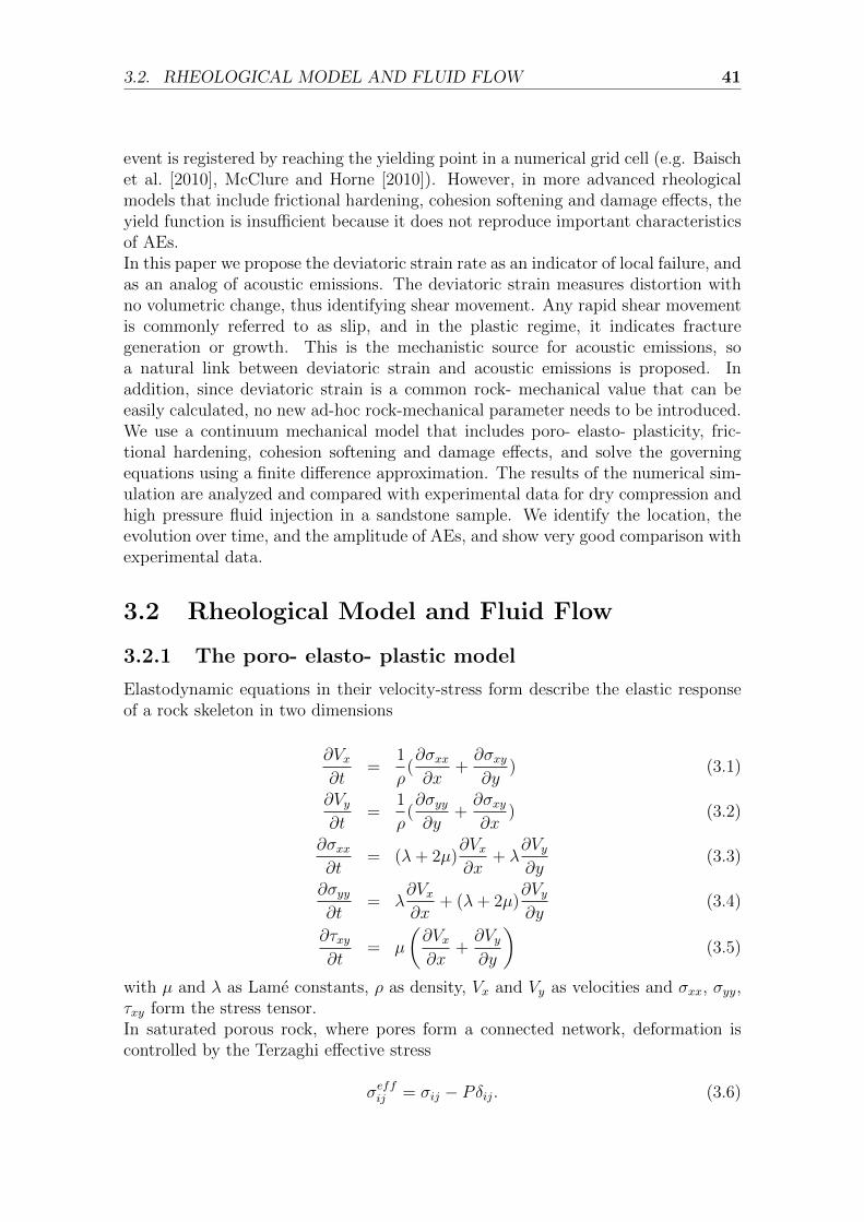
The behavior of a two dimensional rock in the elastic domain is described by theelastodynamic equations:

∂Vx∂t

=1

ρ(∂σxx∂x

+∂σxy∂y

) (2.1)

∂Vy∂t

=1

ρ(∂σyy∂y

+∂σxy∂x

) (2.2)

∂σxx∂t

= (λ+ 2µ)∂Vx∂x

+ λ∂Vy∂y

(2.3)

∂σyy∂t

= λ∂Vx∂x

+ (λ+ 2µ)∂Vy∂y

(2.4)

∂τxy∂t

= µ

(∂Vx∂x

+∂Vy∂y

)(2.5)

where µ and λ are the Lame constants, ρ is the density, Vx and Vy is the velocityvector and σxx, σyy, τxy is the stress tensor.Plastic deformation of rocks is modeled using Mohr-Coulomb criteria

fp = τ −(σm −

C∗

tan(ϕ0)

)· sin(ϕ∗) (2.6)

where fp is the yield function, C∗ is the mobilized cohesion, ϕ∗ is the mobilizedinternal friction angle,ϕ0 is the maximal internal frictional angle, τ is the stressdeviator, σm is the mean stress.Cohesion and internal friction angle are mobilized in terms of a cohesion weakeningand frictional strengthening model (CWFS) in dependence of the effective plasticstrain εp (Hajiabdolmajid et al. [2002]). The mobilized values for friction angle,cohesion and dilatancy angle are calculated following (Vermeer and de Borst [1984]).The plastic strain rates are given by

εplij = 0 for fp < 0 or fp = 0 and fp < 0 (2.7)

εplij = λp∂q

∂σijfor fp = 0 and fp = 0. (2.8)


with λp is the plastic multiplier and q is the flow rule.The effective plastic strain εp follows from there

εp =

√2

3εpT ·M · εp (2.9)

where M is a weighting matrix (Abbo [1997]).We use non-associative plastic flow rules (Vermeer and de Borst [1984])

q = τ − σm · sin(ψ∗) (2.10)

where ψ∗ is the mobilized dilatancy angle.Using equation 2.7 the hardening parameter εp can be calculated with a functionl(q, σ) using λp

εp = λp · l(q, σ) (2.11)

with

l(q, σ) =

√2

3

∂q

∂σ

T

M∂q

∂σ(2.12)

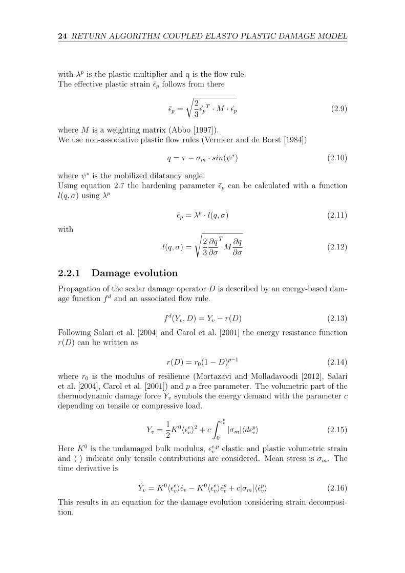
2.2.1 Damage evolution

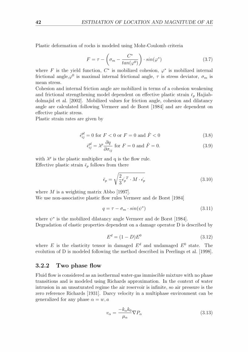
Propagation of the scalar damage operator D is described by an energy-based dam-age function fd and an associated flow rule.

fd(Yv, D) = Yv − r(D) (2.13)

Following Salari et al. [2004] and Carol et al. [2001] the energy resistance functionr(D) can be written as

r(D) = r0(1−D)p−1 (2.14)

where r0 is the modulus of resilience (Mortazavi and Molladavoodi [2012], Salariet al. [2004], Carol et al. [2001]) and p a free parameter. The volumetric part of thethermodynamic damage force Yv symbols the energy demand with the parameter cdepending on tensile or compressive load.

Yv =1

2K0〈εev〉2 + c

∫ εpv

0

|σm|〈dεpv〉 (2.15)

Here K0 is the undamaged bulk modulus, εe,pv elastic and plastic volumetric strainand 〈〉 indicate only tensile contributions are considered. Mean stress is σm. Thetime derivative is

Yv = K0〈εev〉εv −K0〈εev〉εpv + c|σm|〈εpv〉 (2.16)

This results in an equation for the damage evolution considering strain decomposi-tion.

2.2. RHEOLOGICAL MODEL 25

fd =∂fd

∂Y

[K0〈εev〉Iε

−λp(K0〈εev〉

(∂q

∂σxx+

∂q

∂σyy+

∂q

∂σzz

)− c|σm|〈

∂q

∂σxx+

∂q

∂σyy+

∂q

∂σzz〉)]

+∂fd

∂DD = 0

(2.17)

This can be further simplified using Rd =

∂fd

∂Yv∂fd

∂D

=−1

r0 (p− 1) (1−D)p−2 and an

appropriate function m(q, σ).

D = −RdK0〈εev〉Iε+ λpRd

(K0〈εev〉m(q, σ)− c|σm|〈m(q, σ)〉

)(2.18)

where

m(q, σ) =∂q

∂σxx+

∂q

∂σyy+

∂q

∂σzz(2.19)

With presence of damage, the elastic relationship with the elasticity tensor E

σ = E · εe (2.20)

changes due to stiffness degradation to

σ = Ed · εe = (1−D)E0εe (2.21)

with the damaged and undamaged elasticity tensor Ed = (1−D)E0.

2.2.2 Elasto-plastic damage coupling

Based on elasto- plastic and damage equations a system of two linear equations isfound for the two parameter λp and D. It can be solved with Cramer’s rule for twounknowns with a general plastic denominator

Pdenom =

(∂f p

∂σ

T

Ed ∂q

∂σ− ∂f p

∂κl(q, σ)

)+Rd

(K0〈εev〉m(q, σ)− c|σm|〈m(q, σ)〉

)·(

∂f p

∂σ

T

E0εe) (2.22)

to

λp =

∂fp

∂σ

TEdε+

(∂fp

∂σ

TE0εe

)·RdK

0〈εev〉Iε

Pdenom(2.23)

Equation 2.18 can be used to calculate D for a known λp.


2.3 Numerical Algorithm

In the absence of damage, various numerical integration schemes can be found inliterature (e.g. Abbo [1997], Sloan et al. [2001], Crisfield [1991]). The fundamentalstructure of our algorithm is based on the elastic predictor - plastic corrector scheme.In the elastic predictor - plastic corrector scheme an elastic deformation is assumedat first. If this step causes an illegal stress state fp > 0, only the elastic part belowthe yield function,fp < 0, is considered. The other part of the predictor step is usedto calculate the plastic stress. A detailed description of the algorithm can be foundin Abbo [1997] and Sloan et al. [2001].As we consider damage, each part of the predictor step, elastic and plastic, is deter-mined without any change in damage. The stress and strain values after the elasticdeformation, and again after the plastic deformation, are tested with the damagefunction. If damage evolution takes place, prior stress values are corrected (elasticdomain) or re-calculated (plastic domain) considering damage evolution.In general, 4 cases have to be separated:

• purely elastic fp < 0 and fd < 0

• elastic + damage fp < 0 and fd ≥ 0

• purely plastic (elastic content handled extra) fp ≥ 0 and fd < 0

• plastic + damage fp ≥ 0 and fd ≥ 0

The complete overall algorithm is detailed below (see also figure 2.1):

1. Enter with stress σn, strain increment ∆ε and hardening parameter κn with nindicating the prior time step.

2. Calculate the elastic stress increment as part of the elastic predictor: ∆σen+1 =Edn∆ε.

3. Test the trial stress σtrial = σn + ∆σen+1 in the yield function fp.

• If fp > 0 calculate the intersection α with the yield surface followingAbbo [1997] and set σn+1 = σn + α∆σen+1 and ∆ε = (1− α)∆ε.

4. Update 〈εev〉.

5. Test the damage function fd with the updated 〈εev〉.

• If fd ≥ 0 update the damage coefficient Dn+1 using equation 2.18 withλp = 0 and update elastic tangent matrix Ed. Correct recent stress withσn+1 = σn · 1−Dn+1

1−Dn (Shao et al. [2006], Salari et al. [2004]).

6. Calculate plastic stress, if fp ≥ 0 with

λp =E0 ∂gp

∂σ∂fp

∂σ

TE0(

∂fp

∂σ

TEd ∂g

p

∂σ− ∂fp

∂κl(gp, σ)

) (2.24)

See detailed algorithm e.g. in Sloan et al. [2001].

2.4. YIELD- AND DAMAGE- SURFACE RETURN ALGORITHM 27

7. Update the plastic contribution in Yv and test fd again.

• If fd ≥ 0 withdraw results from step 6 and use equations 2.18 and 2.23 tocalculate coupled plastic stresses and damage evolution. Update elastictangent matrix Ed. See detailed algorithm below.

In numerical continuum mechanics it is reasonable to let D asymptotically approach1 (Mortazavi and Molladavoodi [2012]). This can easily achieved by changing theresistance part in fd to

r(D) = r0(Γ−D)p−1 (2.25)

with Γ ≤ 1.

2.4 Yield- and Damage- surface return algorithm

Potts and Gens [1985] and Crisfield [1991] pointed out that the small numericalinaccuracy at determining fp = 0 is additive at every time step and causes wrongresults in the stress space. The standard algorithm to prevent yieldsurface drift,if damage is neglected or weakly coupled, contains two mechanisms: consistent andnormal correction. The consistent correction conserves plastic strain and modifiesthe hardening parameter. It is the preferred structure but does not converge un-conditionally. If the consistent correction fails, the unconditionally stable normalcorrection is applied, which corrects the stresses back to the yield surface in thenormal direction (Abbo [1997], Crisfield [1991]).

We adopt both correction schemes of the purely plastic case for the coupled plastic-damage model. The surfaces can be approximated using Taylor expansion for firstorder terms.

fp = fp0 +∂f p

∂σδσ +

∂f p

∂κδκ (2.26)

fd = fd0 +∂fd

∂YvδYv +

∂fd

∂DδD (2.27)

We use similar relationships as above while keeping the strain constant (δε = 0)

δσ = −δλpEd∂gp

∂σ− δDE0εe (2.28)

δκ = δλp l(gp, σ) (2.29)

δYv = −δλp(K0〈εv〉m(gp, σ)− c|σm|〈m(gp, σ)〉

)(2.30)

A linear system for the two unknowns δλp and δD can be formulated.


Enter withσn, ∆ε, κn

Calculate∆σen+1

Testfp(σn + ∆σen+1;κn) > 0

Calculate Intersectionσn+1 = σn + α∆σen+1

∆ε = (1− α)∆ε∆σ = (1− α)∆σen+1

σn+1 = σn + σen+1

Update 〈εev〉and test fd > 0

Update 〈εev〉and test fd > 0

Update D using equ. 17update Ed

σn+1 = σn ·1−Dn+1

1−Dn

Update D using equ. 17update Ed

σn+1 = σn ·1−Dn+1

1−Dn

Calculate plastic stresswith ∆σ and ∆ε

following e.g. Sloan et al. [2001]

Update Yv and test fd > 0

Withdraw plastic stresses,use coupled

plasticdamage modelwith equations 2.18 and 2.23

and return algorithm

n = n+ 1

yesno

no

noyes yes

no

yes

Figure 2.1: Flowchart for the overall algorithm. Considering all four possible cases:purely elastic, elastic- damage, purely damage, coupled plasticdamage. Elastic andplastic steps are separated using an elastic predictor and determing the intersection of itwith the yield function. The coupled plasticdamage case is discussed later in the text indetail.

2.4. YIELD- AND DAMAGE- SURFACE RETURN ALGORITHM 29

fp0 = δλp(∂f p

∂σ

T

E∂gp

∂σ− ∂f p

∂κl(gp, σ)

)+ δD

(∂f p

∂σ

T

E0εe)

(2.31)

−fd0∂fd

∂D

= δλp (−Rd)(K0〈εv〉m(gp, σ)− c|σm|〈m(gp, σ)〉

)+ δD (2.32)

The system is solved using Cramer’s law.

δλp =

fp0 +fd0∂fd

∂D

(∂fp

∂σ

TE0εe

)Pdenom

(2.33)

Now we determine stresses, hardening parameter and damage operator.

δD =−fd0∂fd

∂D

+ δλpRd

(K0〈εv〉m(gp, σ)− c|σm|〈m(gp, σ)〉

)(2.34)

δσ = −δλpEd∂gp

∂σ− δDE0εe (2.35)

δκ = δλpl(gp, σ) (2.36)

Similar to plastic correction without damage, this correction does not converge un-conditionally. For this case a normal correction has to be applied for both yieldsurfaces as well. Again we assume the stress change to be normal to the plasticyield surface while the hardening parameter as well as the damage operator remainunchanged.We adopt the equation for the correction of the plastic multiplier and the stress:

δσ = −δλp∂fp

∂σ(2.37)

δλp =fp0

∂fp

∂σ

T ∂fp

∂σ

(2.38)

The damage surface is effected because its conjugated thermodynamic force is cor-rected.

δYv = −δλp(K0〈εv〉m(gp, σ)− c|σm|〈m(gp, σ)〉

)(2.39)

As mentioned, the damage operator remains unchanged.The algorithm for the coupled damage- plastic case is detailed below:

1. Chose the parameter c corresponding to εev.

2. Solve iterative or implicit for λp and D using equations 2.23 and 2.18.

3. Update stresses σ, hardening parameter εp and Yv using equations 2.11 and2.15.


4. Calculate yield- and damage functions fp and fd using equations 2.6 and 2.13.

5. While |fp| > FTOL, where FTOL is a tolerance value around 0, use consistentcorrection.

• Calculate δλp and δD using equations 2.33 and 2.34. Solve iterative orimplicit.

• Correct σ, εp and Yv.

• Calculate yield- and damage functions fp and fd.

• If fp > f pold, where fpold describes the yield function of the stress stateprior to the last correction step, use normal correction.

– Withdraw all results from prior correction step

– Calculate δλp using equation 2.38.

– Correct σ, Yv.

– Calculate yield- and damage functions fp and fd.

This algorithm enables results which are consistent with given conditions for thetolerance regions around damage and yield surface, especially avoiding illegal stressstates. The yield surface is the primary variable because this way the coupled plastic-damage case is similar with the purely plastic case and violating the yield surfacehas found to be more critical for rock behavior.

0 0.1 0.2 0.3 0.4 0.50

5

10

15

20

25

30

35

axial strain [%]

axia

l str

ess

[MP

a]

0 MPa confinment stress2 MPa confinment stress4 MPa confinment stress

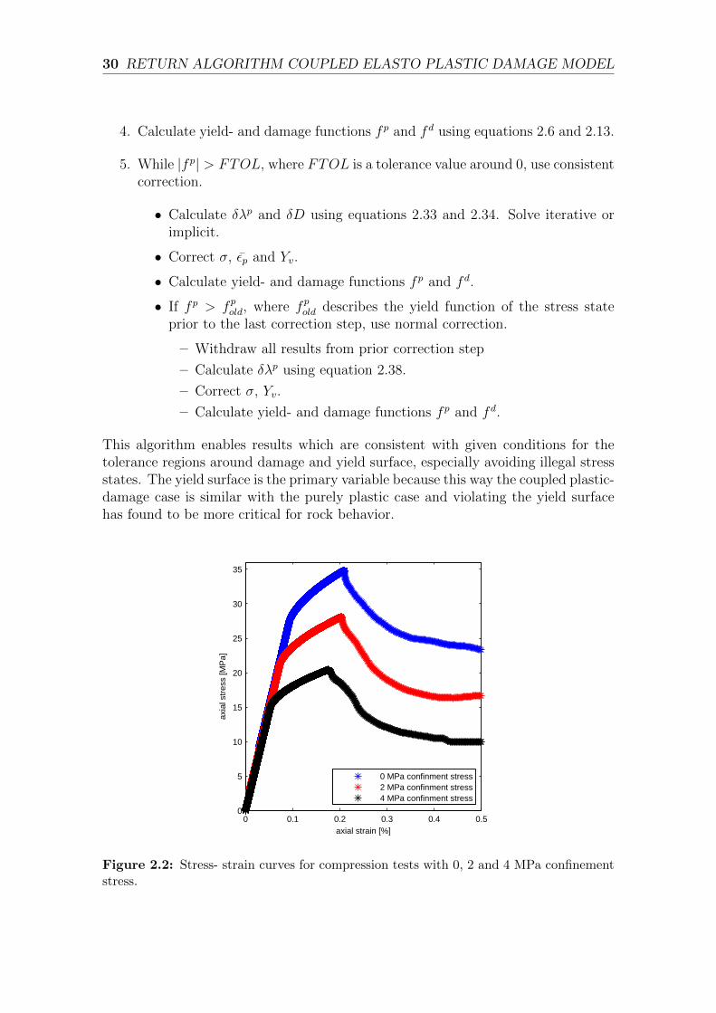
Figure 2.2: Stress- strain curves for compression tests with 0, 2 and 4 MPa confinementstress.

2.5. RESULTS 31

2.5 Results

We compare our simulation to several common experiments with concrete (cf. Wuet al. [2006], Mortazavi and Molladavoodi [2012], Omidi and Lotfi [2010] and others).At first we will present numerical results from confined compression tests and lookinto more detail of the algorithm.

To study the behavior of geomaterial under confined conditions, tests were simulatedwith increasing confinement stress of 2MPa and 4MPa on samples with 6cm diameterand 12cm height with a spatial resolution of 1mm2. The stress strain responsecurve is shown in figure 2.2. The material exhibits larger strength with increasingconfinement stress, which is in good agreement with experimental observations (e.g.Wawersik and Fairhurst [1970]). We will use these tests to study the behavior of thealgorithm in more detail.

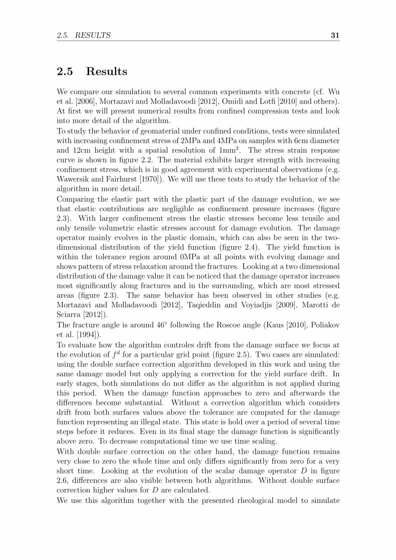
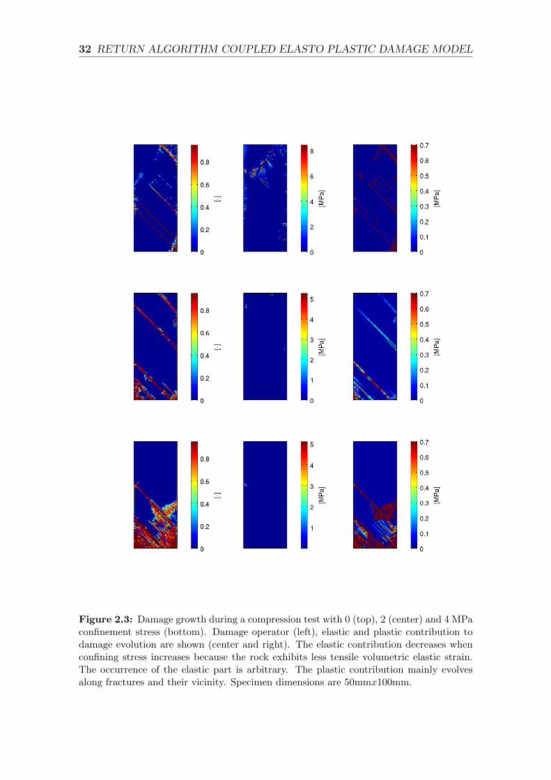
Comparing the elastic part with the plastic part of the damage evolution, we seethat elastic contributions are negligible as confinement pressure increases (figure2.3). With larger confinement stress the elastic stresses become less tensile andonly tensile volumetric elastic stresses account for damage evolution. The damageoperator mainly evolves in the plastic domain, which can also be seen in the two-dimensional distribution of the yield function (figure 2.4). The yield function iswithin the tolerance region around 0MPa at all points with evolving damage andshows pattern of stress relaxation around the fractures. Looking at a two dimensionaldistribution of the damage value it can be noticed that the damage operator increasesmost significantly along fractures and in the surrounding, which are most stressedareas (figure 2.3). The same behavior has been observed in other studies (e.g.Mortazavi and Molladavoodi [2012], Taqieddin and Voyiadjis [2009], Marotti deSciarra [2012]).

The fracture angle is around 46◦ following the Roscoe angle (Kaus [2010], Poliakovet al. [1994]).

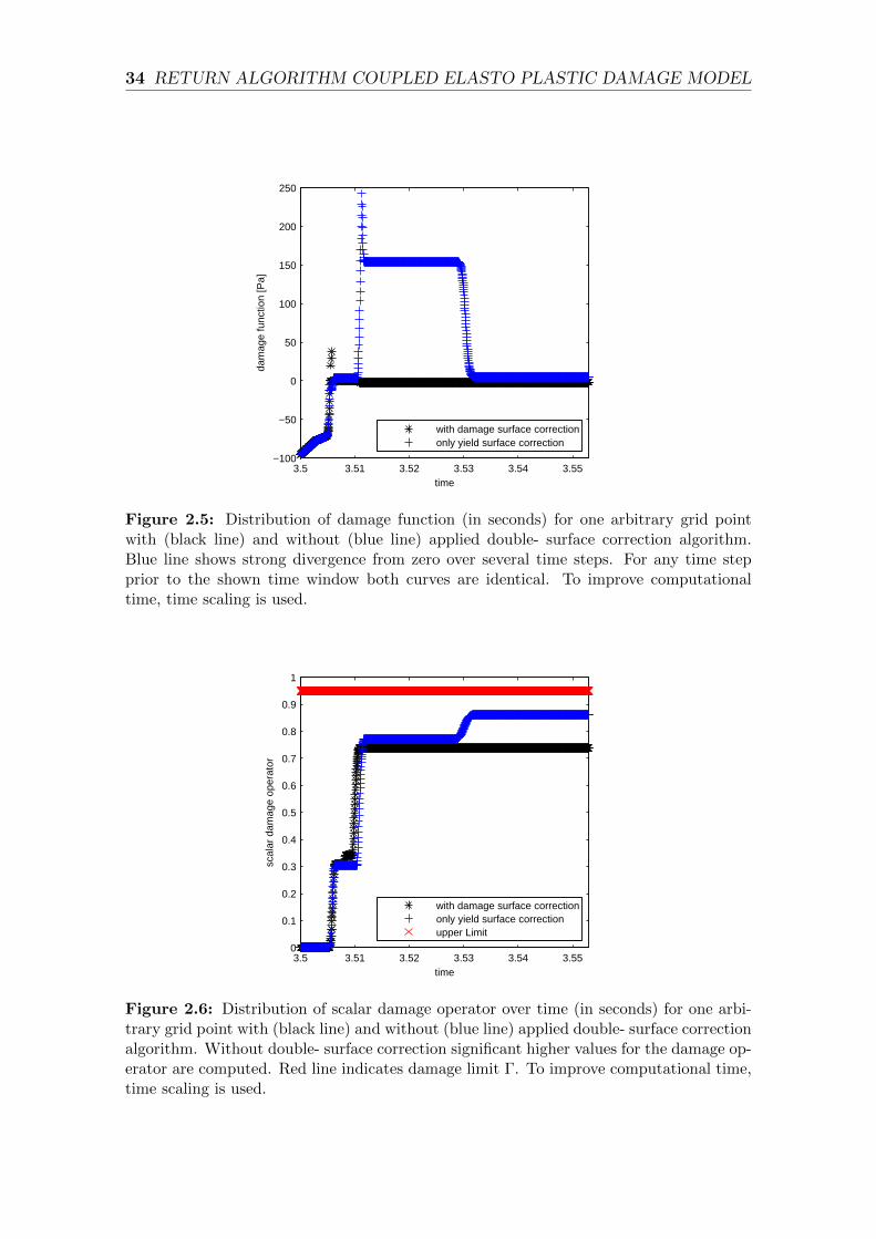
To evaluate how the algorithm controles drift from the damage surface we focus atthe evolution of fd for a particular grid point (figure 2.5). Two cases are simulated:using the double surface correction algorithm developed in this work and using thesame damage model but only applying a correction for the yield surface drift. Inearly stages, both simulations do not differ as the algorithm is not applied duringthis period. When the damage function approaches to zero and afterwards thedifferences become substantial. Without a correction algorithm which considersdrift from both surfaces values above the tolerance are computed for the damagefunction representing an illegal state. This state is hold over a period of several timesteps before it reduces. Even in its final stage the damage function is significantlyabove zero. To decrease computational time we use time scaling.

With double surface correction on the other hand, the damage function remainsvery close to zero the whole time and only differs significantly from zero for a veryshort time. Looking at the evolution of the scalar damage operator D in figure2.6, differences are also visible between both algorithms. Without double surfacecorrection higher values for D are calculated.

We use this algorithm together with the presented rheological model to simulate


Figure 2.3: Damage growth during a compression test with 0 (top), 2 (center) and 4 MPaconfinement stress (bottom). Damage operator (left), elastic and plastic contribution todamage evolution are shown (center and right). The elastic contribution decreases whenconfining stress increases because the rock exhibits less tensile volumetric elastic strain.The occurrence of the elastic part is arbitrary. The plastic contribution mainly evolvesalong fractures and their vicinity. Specimen dimensions are 50mmx100mm.

2.5. RESULTS 33

Figure 2.4: Yield and damage function during a compression test with 2 MPa confine-ment stress. High values of the damage function coincide with a damage operator higherthan 0 and strong plastic contributions along the fracture lines and in surrounding areas.Fracture pattern and stress distribution follows the predicted pattern. Stress relaxationcan be seen around the fractures which is related to more negative values of the yieldfunction.


3.5 3.51 3.52 3.53 3.54 3.55−100

−50

0

50

100

150

200

250

time

dam

age

func

tion

[Pa]

with damage surface correctiononly yield surface correction

Figure 2.5: Distribution of damage function (in seconds) for one arbitrary grid pointwith (black line) and without (blue line) applied double- surface correction algorithm.Blue line shows strong divergence from zero over several time steps. For any time stepprior to the shown time window both curves are identical. To improve computationaltime, time scaling is used.

3.5 3.51 3.52 3.53 3.54 3.550

0.1

0.2

0.3

0.4

0.5

0.6

0.7

0.8

0.9

1

time

scal

ar d

amag

e op

erat

or

with damage surface correctiononly yield surface correctionupper Limit

Figure 2.6: Distribution of scalar damage operator over time (in seconds) for one arbi-trary grid point with (black line) and without (blue line) applied double- surface correctionalgorithm. Without double- surface correction significant higher values for the damage op-erator are computed. Red line indicates damage limit Γ. To improve computational time,time scaling is used.

2.5. RESULTS 35

0 0.1 0.2 0.3 0.4 0.50

5

10

15

20

25

30

axial Strain [%]

axia

l Str

ess

[MP

a]

simulationKarsan & Jirsa, 1969

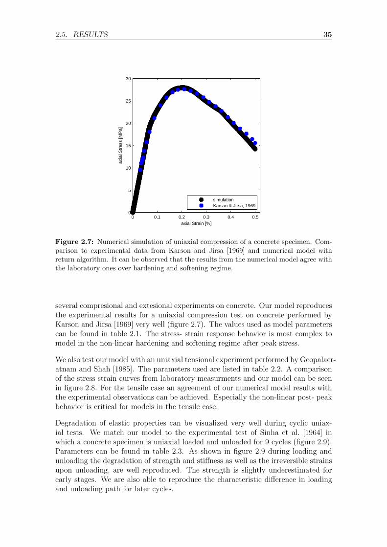
Figure 2.7: Numerical simulation of uniaxial compression of a concrete specimen. Com-parison to experimental data from Karson and Jirsa [1969] and numerical model withreturn algorithm. It can be observed that the results from the numerical model agree withthe laboratory ones over hardening and softening regime.

several compresional and extesional experiments on concrete. Our model reproducesthe experimental results for a uniaxial compression test on concrete performed byKarson and Jirsa [1969] very well (figure 2.7). The values used as model parameterscan be found in table 2.1. The stress- strain response behavior is most complex tomodel in the non-linear hardening and softening regime after peak stress.

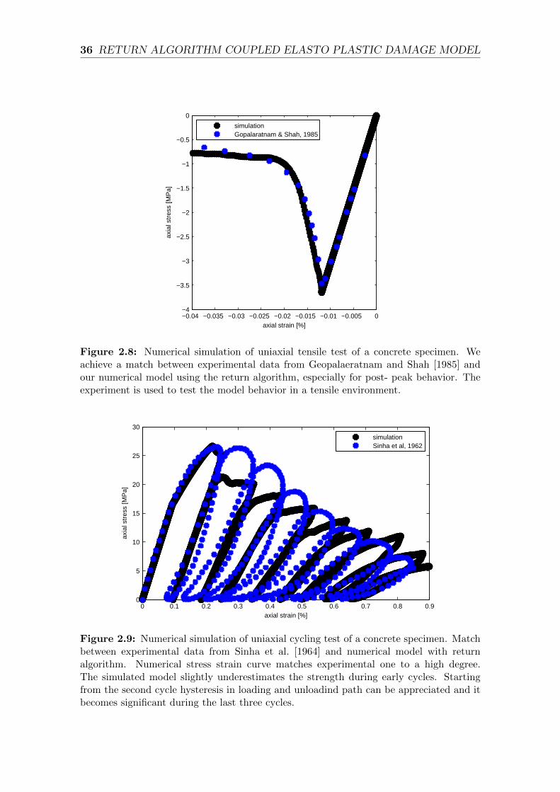
We also test our model with an uniaxial tensional experiment performed by Geopalaer-atnam and Shah [1985]. The parameters used are listed in table 2.2. A comparisonof the stress strain curves from laboratory measurments and our model can be seenin figure 2.8. For the tensile case an agreement of our numerical model results withthe experimental observations can be achieved. Especially the non-linear post- peakbehavior is critical for models in the tensile case.

Degradation of elastic properties can be visualized very well during cyclic uniax-ial tests. We match our model to the experimental test of Sinha et al. [1964] inwhich a concrete specimen is uniaxial loaded and unloaded for 9 cycles (figure 2.9).Parameters can be found in table 2.3. As shown in figure 2.9 during loading andunloading the degradation of strength and stiffness as well as the irreversible strainsupon unloading, are well reproduced. The strength is slightly underestimated forearly stages. We are also able to reproduce the characteristic difference in loadingand unloading path for later cycles.


−0.04 −0.035 −0.03 −0.025 −0.02 −0.015 −0.01 −0.005 0−4

−3.5

−3

−2.5

−2

−1.5

−1

−0.5

0

axial strain [%]

axia

l str

ess

[MP

a]

simulationGopalaratnam & Shah, 1985

Figure 2.8: Numerical simulation of uniaxial tensile test of a concrete specimen. Weachieve a match between experimental data from Geopalaeratnam and Shah [1985] andour numerical model using the return algorithm, especially for post- peak behavior. Theexperiment is used to test the model behavior in a tensile environment.

0 0.1 0.2 0.3 0.4 0.5 0.6 0.7 0.8 0.90

5

10

15

20

25

30

axial strain [%]

axia

l str

ess

[MP

a]

simulationSinha et al, 1962

Figure 2.9: Numerical simulation of uniaxial cycling test of a concrete specimen. Matchbetween experimental data from Sinha et al. [1964] and numerical model with returnalgorithm. Numerical stress strain curve matches experimental one to a high degree.The simulated model slightly underestimates the strength during early cycles. Startingfrom the second cycle hysteresis in loading and unloadind path can be appreciated and itbecomes significant during the last three cycles.

2.6. DISCUSSION AND CONCLUSION 37

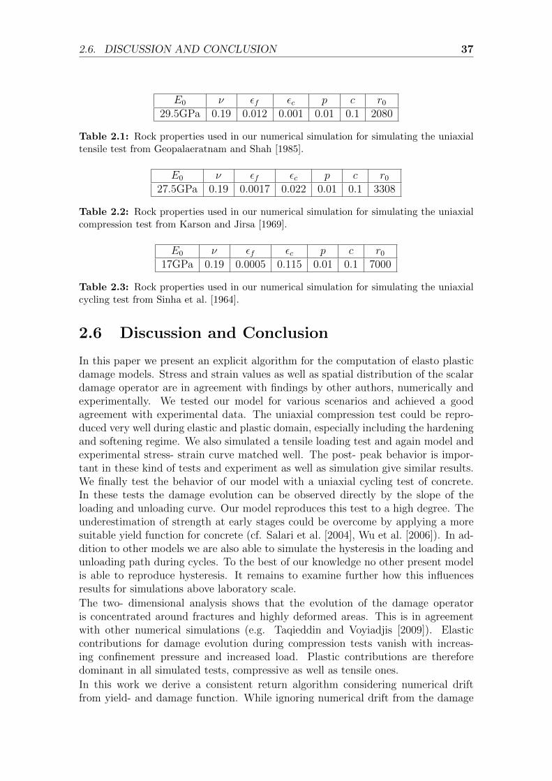
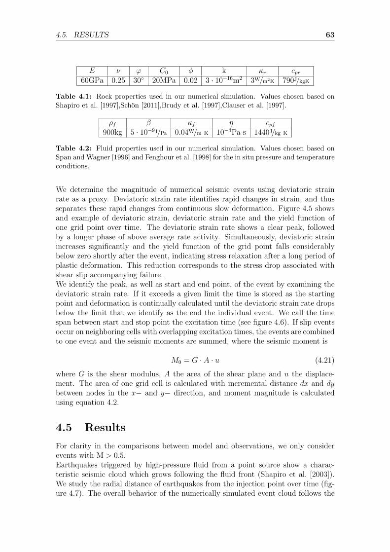
E0 ν εf εc p c r0

29.5GPa 0.19 0.012 0.001 0.01 0.1 2080

Table 2.1: Rock properties used in our numerical simulation for simulating the uniaxialtensile test from Geopalaeratnam and Shah [1985].


27.5GPa 0.19 0.0017 0.022 0.01 0.1 3308

Table 2.2: Rock properties used in our numerical simulation for simulating the uniaxialcompression test from Karson and Jirsa [1969].


17GPa 0.19 0.0005 0.115 0.01 0.1 7000

Table 2.3: Rock properties used in our numerical simulation for simulating the uniaxialcycling test from Sinha et al. [1964].

2.6 Discussion and Conclusion

In this paper we present an explicit algorithm for the computation of elasto plasticdamage models. Stress and strain values as well as spatial distribution of the scalardamage operator are in agreement with findings by other authors, numerically andexperimentally. We tested our model for various scenarios and achieved a goodagreement with experimental data. The uniaxial compression test could be repro-duced very well during elastic and plastic domain, especially including the hardeningand softening regime. We also simulated a tensile loading test and again model andexperimental stress- strain curve matched well. The post- peak behavior is impor-tant in these kind of tests and experiment as well as simulation give similar results.We finally test the behavior of our model with a uniaxial cycling test of concrete.In these tests the damage evolution can be observed directly by the slope of theloading and unloading curve. Our model reproduces this test to a high degree. Theunderestimation of strength at early stages could be overcome by applying a moresuitable yield function for concrete (cf. Salari et al. [2004], Wu et al. [2006]). In ad-dition to other models we are also able to simulate the hysteresis in the loading andunloading path during cycles. To the best of our knowledge no other present modelis able to reproduce hysteresis. It remains to examine further how this influencesresults for simulations above laboratory scale.

The two- dimensional analysis shows that the evolution of the damage operatoris concentrated around fractures and highly deformed areas. This is in agreementwith other numerical simulations (e.g. Taqieddin and Voyiadjis [2009]). Elasticcontributions for damage evolution during compression tests vanish with increas-ing confinement pressure and increased load. Plastic contributions are thereforedominant in all simulated tests, compressive as well as tensile ones.

In this work we derive a consistent return algorithm considering numerical driftfrom yield- and damage function. While ignoring numerical drift from the damage


yield surface is a common practice in numerical rock mechanics, we show that instrongly coupled double surface models this may lead to an overestimation of thedamage variable and a consequent overestimation of the elastic degradation. Toavoid this, algorithms that return the values of the stresses and damage variableto the yield functions must be applied. The presented algorithm is able to preventnumerical drift from damage and yield surface and avoids illegal damage states forcompressional and tensional cases.

Acknowledgment

We thank the German Research Foundation, Deutsche Forschungsgemeinschaft (DFG),for the financial support through the project no. MI 1237/7-1 and the VW founda-tion through the grant ’Extreme Events’.

Chapter 3

A new method to estimate theoccurrence and magnitude ofsimulated rock failure events

Abstract

Predicting failure is one of the primary objectives in the mechanical descriptionof geomaterials. Many different methods have been developed on laboratory andfield scales to measure, identify and isolate trademarks or characteristics of thefailure process. At the laboratory scale, identifying and localizing acoustic emissions(AE) is a common method for the short term prediction of failure. Above averageAE typically precedes the failure process and is easily measured. At larger scales,increase in micro-seismic or seismic activity sometimes precedes large earthquakes(e.g. Tohoku, L’Aquilla, oceanic transforms), and can be used to assess seismic risk.The goal of this work is to develop a methodology and numerical algorithms forextracting a measurable quantity analogous to AE arising from the solution of equa-tions governing rock deformation. Since there is no physical quantify of AE derivablefrom the governing equations, then an appropriate rock-mechanical analog has tobe found. In this work, we identify a general behavior of the AE generation processpreceding rock failure. This behavior includes an arbitrary localization of low mag-nitude events during the pre-failure stage, followed by increases in both the numberand amplitude, and finally localization around the incipient failure plane duringmacroscopic failure. We propose deviatoric strain rate as the numerical analog thatmimics this behavior, and develop two different algorithms designed to detect rapidincreases in deviatoric strain using short-term and long-term moving averages.The numerical model solves a poroelasto- plastic continuum model and is coupledto a two- phase flow model using Richards approximation. We test our modelby comparing simulation results with experiments of an uniaxial compression andof fluid injection into critically stressed probes. We find for both cases that theoccurrence and amplitude of our AE analog mimics the observed general behaviorof the AE generation process. Our technique can be extended to the field scale, thusproviding a mechanistic basis for seismic hazard assessment.

40 ESTIMATION OF LOCATION AND MAGNITUDE OF AE

3.1 Introduction

Understanding failure and rupture processes in geomaterials is one of the primarygoals in earth sciences and engineering. Actively inducing seismicity is finding manyapplications in enhanced geothermal systems and the extraction of hydrocarbonsfrom tight shales, while natural seismicity has long been studied to try and un-derstand the earthquake process and behaviors indicative of impending failure in alarge event. A variety of studies at the field scale focused on the interaction betweenfluid (and fluid pressure) propagation and location of seismic events (e.g. Mayr et al.[2011], Baisch et al. [2010], McClure and Horne [2010]), with acoustic emissions (AE)acting as their laboratory scale equivalent. Acoustic emissions and seismic eventshave similar source mechanisms, but a different range of frequencies (Mogi [1967],Cai et al. [2007]), while both often precede and accompany plastic deformation andchanges of mechanical properties. Observations of seismic and acoustic events areutilized as a predictor of rock failure and rock burst (e.g. Lockner [1993], Pettittet al. [2002]). Modern laboratory techniques allow the detection and localization ofacoustic emissions at very high rates and accuracy, with the rate of recorded sig-nals increasing from hundreds to thousands of events per second over the last fewyears (e.g. Stanchits et al. [2011], Amitrano [2003]). Acoustic emissions analysis isperformed on wide range of materials, including metals (e.g. Farrelly et al. [2004],Marfo et al. [2013], Aggelis et al. [2011], Huang et al. [1998], Sind et al. [2012],Oh and Han [2012]), ceramics (e.g. Mei et al. [2013], Maillet et al. [2014], Aggeliset al. [2013], Yonezu and Chen [2014], Drozdov [2014], Drozdov [2013]), polymers(e.g. Sause et al. [2013],Berdowski et al. [2013], Fu et al. [2014], Hamdi et al. [2013],Njuohvic et al. [2014], Boominathan et al. [2014], Burks and Kumosa [2014]), andconcrete (e.g. Zhu et al. [2010], Itturrioz et al. [2013], Elfergani et al. [2013], Ohnoet al. [2014], Hu et al. [2013], Kencanawati et al. [2013], Kawasaki et al. [2013],Shahidan et al. [2013], ElBatanouny et al. [2014]).

AE can not be derived directly from physical properties in numerical simulations, soanalogs are needed. Some theoretical approaches exist for discrete element modeling(DEM), where the material is represented by discrete bonded particles that interactwith each other, and exceeding the bond strength is used as the AE analog (e.g.Kun et al. [2014], Hazzard et al. [2002], Hazzard and Young [2002], Hazzard andYoung [2004]). However, DEM are computationally expensive, and have no inherentlength scale necessary to quantitatively compare with observations, thus limitingtheir utility.

Continuum formulation of the underlying mechanics has the advantage that mostof the parameters can be obtained form experimental data, however, an appropriateAE analog must still be found. Some methods have been proposed to characterizeAE in continuum mechanical models, such as the evolution of a damage functionacting on the elastic properties of the rock material (e.g. Amitrano et al. [1999],Amitrano [2003], Fang and Harrison [2002], Lyakhovsky et al. [1997], Tang [1997],Tang and Kaiser [1998], Wang et al. [2012]). For simple fluid-rock interactions, anevent is registered if the pore pressure exceeds some predefined critical value (e.g.Parotidis et al. [2003], Parotidis et al. [2005]), while for simple plastic models and

3.2. RHEOLOGICAL MODEL AND FLUID FLOW 41

event is registered by reaching the yielding point in a numerical grid cell (e.g. Baischet al. [2010], McClure and Horne [2010]). However, in more advanced rheologicalmodels that include frictional hardening, cohesion softening and damage effects, theyield function is insufficient because it does not reproduce important characteristicsof AEs.In this paper we propose the deviatoric strain rate as an indicator of local failure, andas an analog of acoustic emissions. The deviatoric strain measures distortion withno volumetric change, thus identifying shear movement. Any rapid shear movementis commonly referred to as slip, and in the plastic regime, it indicates fracturegeneration or growth. This is the mechanistic source for acoustic emissions, soa natural link between deviatoric strain and acoustic emissions is proposed. Inaddition, since deviatoric strain is a common rock- mechanical value that can beeasily calculated, no new ad-hoc rock-mechanical parameter needs to be introduced.We use a continuum mechanical model that includes poroelasto- plasticity, fric-tional hardening, cohesion softening and damage effects, and solve the governingequations using a finite difference approximation. The results of the numerical sim-ulation are analyzed and compared with experimental data for dry compression andhigh pressure fluid injection in a sandstone sample. We identify the location, theevolution over time, and the amplitude of AEs, and show very good comparison withexperimental data.

3.2 Rheological Model and Fluid Flow

3.2.1 The poroelasto- plastic model

Elastodynamic equations in their velocity-stress form describe the elastic responseof a rock skeleton in two dimensions

∂Vx∂t

=1

ρ(∂σxx∂x

+∂σxy∂y

) (3.1)

∂Vy∂t

=1

ρ(∂σyy∂y

+∂σxy∂x

) (3.2)

∂σxx∂t

= (λ+ 2µ)∂Vx∂x

+ λ∂Vy∂y

(3.3)

∂σyy∂t

= λ∂Vx∂x

+ (λ+ 2µ)∂Vy∂y

(3.4)

∂τxy∂t

= µ

(∂Vx∂x

+∂Vy∂y

)(3.5)

with µ and λ as Lame constants, ρ as density, Vx and Vy as velocities and σxx, σyy,τxy form the stress tensor.In saturated porous rock, where pores form a connected network, deformation iscontrolled by the Terzaghi effective stress

σeffij = σij − Pδij. (3.6)


Plastic deformation of rocks is modeled using Mohr-Coulomb criteria

F = τ −(σm −

C∗

tan(ϕ0)

)· sin(ϕ∗) (3.7)

where F is the yield function, C∗ is mobilized cohesion, ϕ∗ is mobilized internalfrictional angle,ϕ0 is maximal internal frictional angle, τ is stress deviator, σm ismean stress.Cohesion and internal friction angle are mobilized in terms of a cohesion weakeningand frictional strengthening model dependent on effective plastic strain εp Hajiab-dolmajid et al. [2002]. Mobilized values for friction angle, cohesion and dilatancyangle are calculated following Vermeer and de Borst [1984] and are dependent oneffective plastic stress.Plastic strain rates are given by

εplij = 0 for F < 0 or F = 0 and F < 0 (3.8)

εplij = λp∂q

∂σijfor F = 0 and F = 0. (3.9)

with λp is the plastic multiplier and q is the flow rule.Effective plastic strain εp follows from there

εp =

√2

3εpT ·M · εp (3.10)

where M is a weighting matrix Abbo [1997].We use non-associative plastic flow rules Vermeer and de Borst [1984]

q = τ − σm · sin(ψ∗) (3.11)

where ψ∗ is the mobilized dilatancy angle Vermeer and de Borst [1984].Degradation of elastic properties dependent on a damage operator D is described by

Ed = (1−D)E0 (3.12)

where E is the elasticity tensor in damaged Ed and undamaged E0 state. Theevolution of D is modeled following the method described in Peerlings et al. [1998].

3.2.2 Two phase flow

Fluid flow is considered as an isothermal water-gas immiscible mixture with no phasetransitions and is modeled using Richards approximation. In the context of waterintrusion in an unsaturated regime the air reservoir is infinite, so air pressure is thezero reference Richards [1931]. Darcy velocity in a multiphase environment can begeneralized for any phase α = w, a

vα =−kαk0

µα∇Pα (3.13)

3.3. ALGORITHM TO DETECT AN ANALOG FOR AE DURINGCONTINUUM NUMERICAL SIMULATIONS 43

where k0 is intrinsic permeability, µα is phase viscosity, kα is phase permeability andP is pressure. Phase permeability varies between 0 and 1. It can be linked to the sat-uration S using vanGenuchten relationships, which show very good agreement withexperimental data for water and air mixture (Cropper et al. [2011],vanGenuchten[1980]).

kw =√Sw

(1−

(1− S

1mw

)m)2

ka = (1− Sw)2 ·(

1− S2+3mm

w

) (3.14)

The Richards equation remains.

∂Pw∂t

=1

φ(Sw · cw + ∂Sw

∂Pw

)∇(kwk0

µw∇Pw

)(3.15)

3.3 Algorithm to detect an analog for AE during

continuum numerical simulations

Frictional movement along preexisting cracks or generation of new fractures gener-ate acoustic emissions during plastic deformation in laboratory scales (Fortin et al.[2009], Zang et al. [1996], Lisjak et al. [2013]), while the same processes generateseismic events in field scales. Therefore, acoustic emissions behave similar to seis-mic events in many characteristics like propagation, energy release and generationmechanisms but differ in frequencies of seismic waves (Cai et al. [2007]).Seismic wave amplitude is correlated to seismic moment Itturrioz et al. [2013], wherethe scalar seismic moment is defined as

M0 = G · A · u (3.16)

where G is the shear modulus, A the area of the shear plane and u the displacementand seismic moment magnitude is determined by the empirical relation

Mw =2

3log10 (M0)− 6 (3.17)

Estimating seismic moment in a numerical simulation requires determining only thearea of slip A and displacement u because the shear modulus is known. In a finitedifference scheme, the smallest area of slip that can be resolved is the grid cell sizedx · dy with an incremental distance dx and dy between nodes in the x− and y−direction. The total area of an event will be given by the combined area of the cellsthat fail in a common spatial and time window. We make the spatial constraint thatonly immediate neighbor cells can combine their areas because stress transfer cantrigger failure from one cell to the immediate neighborhood. The slipping regioncan propagate from one cell to the others and generate a cluster of simultaneouslyfailing. We add the area of all cells of this cluster and define a spatial window. We


define an excitation time window as the time span from the initial slipping of onecell of the cluster until the end of the slipping of the last excited cell of the cluster.During this time new areas are combined to one common event (see figure 3.1).Anything outside this time window is counted as a separated event. It is certainlytrue that slip anywhere transfers stress to the immediate neighborhood and cantrigger further slip, but if this new event is not within certain time window, it isregistered a separate events the slip do not contribute to the magnitude of the priorevent.

excitation time 1

excitation time 2

excitation time 3excitation time 4

cell1

overall excitation time

x

t

cell2

cell3 cell

4

Figure 3.1: Defining the excitation time window for a simplified 1d case. Cell 1 startsto slip, which triggers cells 2 and 3. The excitation time of cell 4 does not overlap withone of its neighboring cells, and is considered a single event, Slip of the cells 1, 2 and 3are recorded as one joint event.

The essential purpose of our model is to detect of an event and to determine theamount of slip. We propose the deviatoric strain rate as an analog to AE becausehigh deviatoric strain rates indicate shear failure. Deviatoric strain is defined as:

εdev =

√(εxx − εyy)2

4− ε2xy (3.18)

where εii are normal strains and εij are shear strains. We use the deviatoric strainrate to identify rapid changes in the deviatoric strain and to isolate discontinuousevents from continuous deformation. Figure 3.2 shows the deviatoric strain, thedeviatoric strain rate, and the yield function of one grid point over a time spanthat we identify as an event (shaded time window). The deviatoric strain rateshows a clear peak, followed by a longer phase of above average rate activity, whilesimultaneously the deviatoric strain significantly increases. The yield function of thegrid point falls well below zero shortly after the event, indicating elastic deformationfollowing a long period of plastic deformation during the event. This decrease in theyield function is due to stress drop in the cell associated with shear displacement.We view this substantial reduction in the yield function as a primary argumentthat the increase in deviatoric strain signals failure and can thus be used as an AEanalog. Other continuum mechanical models that include acoustic emissions do nothave this intrinsic feedback between acoustic emission and the stress state.

No measurable change in the yield function is observed at the onset of slip, butrather small variations (figure 3.2). These high frequency oscillations of the yieldfunction around zero are a result of the applied algorithm to prevent a drift fromthe yield surface (e.g. Abbo [1997], Potts and Gens [1985]). It is not used in the

3.3. ALGORITHM TO DETECT AN ANALOG FOR AE DURINGCONTINUUM NUMERICAL SIMULATIONS 45

Figure 3.2: Deviatoric strain, deviatoric strain rate and yield function over time of onegrid point during a rapid shear movement (marked region).

detection algorithm at any point and does not have any physical meaning. It ispurely numerical noise.

We apply an algorithm that uses a moving average to identify periods of high devi-atoric strain rate. In this method, a short term average (STA) covers a time spanof a part of the length of an expected event, and a long term average (LTA) that isconsiderably longer than the expected event duration. If the ratio

q =STA

LTA(3.19)

exceeds a given limit qlimit, then an event is detected. With an appropriate choiceof the length of STA and LTA, in combination with a value for qlimit, events can bedetected. This method ensures that the increase in deviatoric strain is rapid andthus signals failure.

To determine the slip, the beginning and the end of the excitation time windowneeds to be evaluated. After the peak in the q ratio is found, single points beforethis peak are tested. For this we compute the ratio qp of the previous point untilwe find the first point for which the qp ratio is above a different limit qstart. Thispoint in time is chosen as starting point of the slip. When q drops below anotherlimit qend, we set the end of the time window. In many cases we found it sufficientto choose qstart = qend. Any point inside this time window (and belonging to theclusters of immediate neighbors) contributes to the total slip of the event (see figure3.3),


q

qlimit

qstart

excitation time time

Figure 3.3: Defining the excitation time window for one cell. Initially the peak is detectedwith the STA / LTA ratio q of the deviatoric strain exceeding a defined limit. The startand end points of the slip are found with a much lower limit value. The time during start-and end point gives the excitation time window during which all displacement is summedup for this slip event.

u =

∫ tend

tstart

vdt (3.20)

with displacement u, velocity v and incremental time step dt.

We found this method to be very reliable and robust for detecting rapid changesin deviatoric strain rates. However, the correct setting of the two limits, qlimit andqstart = qend, is necessary to achieve good results. A high qlimit ensures that only realevents are detected as opposed to noise. A low qstart = qend on the other hand enablesproper accounting of the entire slip event. These limits, once determined, are stableagainst variations of the setup such as changes in boundary conditions. However, thismethod is computationally expensive in both memory usage and processing becausefor every cell the LTA and STA values have to be stored with some significant length.The LTA requires significantly more values than the slip itself, and the algorithm iscomputationally intensive due to many arithmetic operations and conditionals.

A faster method with less consumption is to compare the of values of deviatoric strainat consecutive time steps. It is even possible to compare the values within a suitabletime period that reduces computational processing costs even further. Comparingconsecutive values of the deviatoric strain is equivalent to the mean deviatoric strainrate. If the difference between the two values at consecutive times exceeds somepredefined number, an event is detected. The first time step at which the differenceexceeds a predefined value is chosen as the starting point of the excitation timeand as soon as the difference drops below the limit the end of excitation time isreached (see figure 3.4). Slip during this event can be determined in a similar wayto the first method. This second method is substantially faster with smaller memorydemands because for each cell only one additional value, the deviatoric strain of the

3.4. NUMERICAL EXPERIMENTS AND RESULTS 47

previous step, has to be stored. This algorithm is also computationally simple as itcontains only one condition to be tested. However as only one condition remains,this algorithm is more sensitive to the chosen limit value as the same value is usedfor detecting a peak at all and determining the excitation time, which influences themagnitude. The value needs to be high enough so noise is not considered but alsolow enough to cover the whole peak from start to end point. Both algorithms canbe adjusted to give similar results with the limit value of the later algorithm beingbetween the limit values of the more complex algorithm.

devi

ator

ic s

trai

n

excitation time t

not every calculatedtime step is compared

difference betweenboth points is biggerthan the limit

difference betweenboth points is smallerthan the limit

Figure 3.4: Defining the excitation time window for one cell with the faster method.Consecutive values of the deviatoric strain are compared. Not every computed value(black dots) needs to be compared but equally spaced and narrow ones (red circles). Theslip event starts when the difference between two values exceeds a given limit. Excitationtime continues until the difference between two values again drops below the limit.

Detecting failure of a cell during the computation allows other feedback to be dy-namically included, such as permeability increases at the onset of slip, frictionalheating, or other slip-dependent processes.

3.4 Numerical experiments and results

We apply our theoretical and numerical model to two high resolution laboratoryexperiments of hydraulic fracturing of critically stressed rock samples (Stanchitset al. [2011], Mayr et al. [2011]). In these experiments acoustic emissions (AE) wereregistered and located using high precision ultrasonic tomography to link AE to apropagating fluid front. Such correlations between the fluid front and AE had notpreviously been achieved in comparable experiments. The tests were performed onsamples of Flechtingen Sandstone, which can be assumed to be isotropic. Furtherdetails are found in Backers [2004], Stanchits et al. [2011], Blocher et al. [2009]. Forthe injection experiments, water was directly applied to the bottom of the specimen,while the top of the specimens was sealed (Mayr et al. [2011]).


We compare our model results with a confined compression experiment and a fluidinjection in an undrained, critically stressed specimen.We numerically solve the governing equations using a two dimensional finite- dif-ferences scheme with a staggered grid (Saenger et al. [2000]). The model setup ischosen to match the experimental setup described in Stanchits et al. [2011]. Thenumerical model has a spatial resolution of 1mm distance between grid points ineach direction.

0.01 0.02 0.03 0.04 0.05

0.02

0.04

0.06

0.08

0.1

0.12

x− direction [m]

y− d

irect

ion

[m]

0.01 0.02 0.03 0.04 0.05

0.02

0.04

0.06

0.08

0.1

0.12

0.01 0.02 0.03 0.04 0.05

0.02

0.04

0.06

0.08

0.1

0.12

Figure 3.5: Spatial distribution of events over the specimen at different times. The leftfigure shows events at an early stage that are randomly distributed through the domain.The middle picture shows a localization of events around macroscopic failure, which isclearly visible in the right picture showing events registered in the last stage of the experi-ment at macroscopic failure. White points indicate cells with at least one event registeredduring the time span.

3.4.1 Confined compression

In the first part of the experiment, a specimen was compressed with 40MPa confiningpressure and a variable axial load until the onset of macroscopic failure, followed byunloading. The simulation results agree with the experimental data in stress-strainpath, volumetric and inelastic strain as well as fracture nucleation and propagation(Heinze et al. [2015b]).Dry compression experiments reveal several features of AE genesis (Stanchits et al.[2011], Fortin et al. [2009], Lyakhovsky et al. [1997], Amitrano et al. [1999]) thatmust necessarily be reproduced by a numerical simulation analog, including:

• Arbitrary locations in first stages of compression;


23 23.5 24 24.50

50

100

150

200

250

time [s]

AE

act

ivity

[1/s

]

Figure 3.6: Rate of occurrence of acoustic emissions at macroscopic failure. The activityincreases suddenly and stays above average during the development of the macroscopicfailure plane. This is followed by a decline to normal activity.

• Localization surrounding the incipient macroscopic failure plane;

• A rapid increase in the rate of occurrence during macroscopic failure, followedby a rapid decline;

• A rapid increase in AE amplitude during macroscopic failure, followed by arapid decline.

We reproduce all four of these features in our numerical simulations. We find thatevents detected in the early stages of compression are randomly distributed, andfollowed at later stages by localizing around the failure plane and then predominantlyalong the failure plane (figure 3.5). The first emissions are triggered at weak pointsintroduced by a heterogeneous distribution of cohesion and internal friction angle.

The number and magnitude of events signal the onset of macroscopic failure, withthe number of events increasing rapidly and concentrating around the failure plane(figure 3.6). Many events occur because stress concentrates around the fractureplane, so many numerical grid points nearby each other simultaneously reach acritical state. For the same reason, events have a larger magnitude because many gridpoints are slipping simultaneously resulting in a larger slip event. As neighboringcells reach failure, an event is more likely to trigger failure of its neighbors duringits own excitation time so cells combine for one single joint event (figure 3.7).


23 23.5 24 24.50

0.2

0.4

0.6

0.8

1

1.2x 10

−5

time [s]

Dis

plac

emen

t− A

mpl

itude

[m]

Figure 3.7: Magnitude of detected events over time at the moment of macroscopic failure.The magnitude increases rapidly and stays high while macroscopic failure is ongoing andpropagating through the specimen. It declines abruptly after the fracture is completed.

3.4.2 Fluid injection in an undrained rock

Fluid injection into a host rock is widely used in enhanced geothermal systems,waste disposal, CO2 sequestration, and fracking. In each of these processes, acous-tic emissions (e.g. seismicity) is used as a measure of fluid front and is thus of greatinterest. We further test our numerical AE analog with observations from an exper-iment where a rock specimen was sealed at the top and a fluid pressure boundaryof 5MPa was applied to the bottom boundary. The experiments showed a clearcorrelation between the propagating fluid front and location of acoustic emissions(Stanchits et al. [2011]), with AEs mostly detected below or close to fluid front andvery few events in the upper part of the specimen. Field observations show a similarcorrelation between (micro-) seismic events and estimated fluid front (e.g. Shapiroet al. [2003]).

Realistic fits between numerical simulation and experiments require that the fluid be-havior be reproduced. In experiments, the fluid front is estimated from the injectedvolume and fitting the solution of a linear diffusion equations to the AE (Stanchitset al. [2011], Mayr et al. [2011]). On field observations like at geothermal plants thefluid front is estimated from the occurrence of seismic events (e.g. Shapiro et al.[2003], Parotidis et al. [2003]).In the numerical simulation we determine the fluidfront from the saturation equation, and for the simulated experiment the fluid frontin the numerical model agrees well with that estimated from the injected volume,and differs a little from the fluid front derived from the linear diffusion equationsolution (figure 3.8 and Stanchits et al. [2011]).


0 100 200 300 400 500 600 7000

0.02

0.04

0.06

0.08

0.1

0.12

time [s]

heig

ht [m

]

EventsFluid Front of SimulationFluid Front of Experiment (pump volume)Fluid Front of Experiment (fitted to AE)

Figure 3.8: Events occurring during fluid injection obtained from the numerical simu-lation. The behavior agrees very well with the results from laboratory experiments andfrom field observations (cf. Stanchits et al. [2011], Shapiro et al. [2003]). Many events atthe bottom are induced as fluid is injected because the rock is critically stressed and fluidsand poro-elasticity redistributes the stresses. Only a few events are registered above thefluid front, and fewer events occur with time. A general stress drop in the specimen dueto fluid injection results in a non-critically stressed specimen at later times.


0.01 0.02 0.03 0.04 0.05

0.02

0.04

0.06

0.08

0.1

0.12

x− direction [m]

y− d

irect

ion

[m]

Figure 3.9: Points indicate cells that recorded at least one numerical AE. Micro- fracturesbelow the fluid front (red line) are clearly visible, and only a few events are observed abovethe fluid front.

3.5. DISCUSSION AND CONCLUSIONS 53

A clear correlation between the fluid front and the occurrence of events can beobserved in our simulations and in the experimental measurements (figure 3.8).Only few events take place in the upper part of the specimen and also at the bottomfor later times. This is identical to field and laboratory data. In figure 3.9 this isalso clearly visible. The red line marks the fluid front and micro- fractures can beidentified below the fluid front due to the cells which signaled an event. The eventsare triggered by the fluid pressure propagating through the specimen from bottomto top. Fluid injection leads to a general stress drop inside the specimen, so aftersome time the specimen is no longer critically stressed and the event rate subsides.Additionally, if the maximum fluid pressure is reached in a spatial region of thespecimen, failure is unlikely until higher fluid pressures are applied.

3.5 Discussion and Conclusions

We propose deviatoric strain rate as an AE analog value to detect rapid, plasticdeformation along preexisting cracks and the generation of new fractures. With thismethod, we can locate events and determine their seismic moments during the simu-lation. We apply this numerical AE detection method to a fully coupled poroelasto-plastic continuum model that incorporates frictional hardening, cohesion weakeningand damage effects. We compare the results of our method with experimental datafrom a confined compression experiment of an undrained specimen, and with fluidinjection in a critically stressed specimen. Both experiments can be reproduced instress- strain behavior and fluid movement as well as in occurrence and amplitudeof AEs (Heinze et al. [2015b]).We present two different approaches for implementing the method, and both ap-proaches produce similar results when adjusted accordingly.During dry compression, our numerical AE (e.g. deviatoric strain rate) occur ran-domly throughout the model early in the loading, followed by localization aroundthe macroscopic failure plane, similar to experimental observations (Lockner [1993]).Both the amplitude and the number of numerically recorded AE increases signifi-cantly during macroscopic rupture. AE occur during fluid injection near the fluidfront and behind the front, and fade after maximum pressure is reached, results sim-ilar to experimental and field observations. (Stanchits et al. [2011], Shapiro et al.[2003]).These methods are easily adaptable to other simulations and numerical implemen-tations, and we will extend these results to field scale experiments that might allowmechanistic assessment of seismic hazard through a determination of earthquakemagnitude.

Acknowledgment


54 NUMERICAL SIMULAION OF THE 2008 BOHEMIAN EQ SWARM

Chapter 4

Numerical Simulation of the 2008Bohemian Earthquake Swarm

Abstract

CO2 has long been suspected of driving the Bohemian earthquake swarms because ofthe migrating nature of the swarms and expressions of CO2 degassing at the surface.Modelling to date primarily employed linear diffusion models, but more sophisticatedmodelling that includes mechanics has been lacking. In this paper, we apply amodel that couples mechanics to heat and flow of a super-critical CO2 througha fracture network. We present a continuum mechanical approach to derive theseismic moment magnitude using the deviatoric strain as an indicator of rupturingprocesses during individual events. We use a peak- detection algorithm to identifyrapid changes in deviatoric strain, indicative of slip events. This method has beenshown to work very well in dry and fluid-induced fracturing experiments at thelaboratory scale, and in this work we extend the method to the scale of the WestBohemia / Vogtland earthquake swarms. We show very good agreement betweenmodel results and observations of the 2008 swarm, further supporting the hypothesisthat the Bohemian earthquake swarms are predominately fluid-driven.


12 12.2 12.4 12.6 12.849.8

49.9

50

50.1

50.2

50.3

50.4

KTB

Novy Kostel

Eger rift

Marianske Lazne fault

Germany

Czech republic

Figure 4.1: Map of the border region of Germany and Czech republic. Most recentearthquake swarms take place around the city Novy Kostel,which is located close to theMarianske Lazne fault and the Eger- rift system. The German continental deep drillingproject (KTB) is nearby.

4.1 Introduction

The West Bohemia / Vogtland earthquake swarms coincide with degassing of CO2

originating from the mantle. Young Quaternary volcanism with a magmatic bodyassociated with a local up-doming of the Moho is the assumed source for the CO2,which then propagates through a preexisting and re-stimulated fracture networkWeinlich et al. [1999]. The fluids are suggested as the primary trigger for earth-quake activity in the region (e.g. Spicak and Horalek [2001], Weise et al. [2001],Brauer et al. [2003]). Most earthquake swarms over the last decades occurred inthe Novy Kostel area (Czech Republic, see figure 4.1) within a region of severalsquare kilometers. The maximum earthquake magnitude arising from these swarmsis around ML = 3.5, and include several thousands of microseismic events at depthsranging between 6.5 and 11km. Occasionally some deeper events are detected ataround 13km depth, and occur along a steeply dipping fault plane (Fischer and Ho-ralek [2003]). Earthquake swarms were recorded in 1985/1986, 1997, 2000, 2008 and2011, during which pre- fractured areas were reactivated (Fischer et al. [2014]).Estimating the maximum magnitude of seismic events is of great interest in all as-pects of seismic hazard assessment, but has so far been limited to statistical estimatesthat have a very poor record (Geller [2011]). The maximum expected magnitude isof particular interest in cases of stimulation, such as enhanced geothermal systems(EGS), because this can determine the outcome of public acceptance of the project.Numerical simulations are occasionally used to assess seismic hazard, but existingmodels are based on simplified rheology and oversimplified mechanics, leading to awide range of uncertainty (e.g. Baisch et al. [2010], McClure and Horne [2010]).In this work we apply a method based on the deviatoric strain rate, in a sophisticated

4.2. THE 2008 EARTHQUAKE SWARM 57

hydro-mechanical model, to estimate seismic activity (Heinze et al. [2015a]), and usethe 2008 swarm as a suitable test case.

An earthquake swarm is defined as a sequence without a single, dominant event(Yamashita [1998]). Field observations and numerical simulations suggest that fluidflow is an important component in the generation of earthquake swarms (Hainzl[2004]). Several numerical models have been applied to the West- Bohemian earth-quake swarms, including a poroelasto plastic finite element model to calculatestresses and strains (Kurz et al. [2003]). These studies demonstrated that the re-gional stress field is insufficient to cause earthquake swarms, but when combinedwith fluid migration they show reasonable rates of deformation capable to causeearthquake swarms. Statistical approaches can reproduce the seismic pattern of the2000 earthquake swarm (Hainzl [2004]), where a brittle patch surrounded by anelastic half- space is loaded by fluid migration and stress changes. The spatio- tem-poral distribution of the seismic events is dominated by stress triggering, with fluidmigration acting as the initiator. Linear diffusion models (Parotidis et al. [2005])focused on a single fluid source to determine overall diffusivity.

Identifying the location and magnitude of numerical seismic events is not straightfor-ward because there is no specific physical value which describes them. Some studieswere performed for geothermal systems using a block- spring model approach to es-timate seismic events and their magnitude (Baisch et al. [2010], McClure and Horne[2010]). In these models seismic events are calculated using an over-simplified phys-ical model.

In this work we develop and apply a model to simulate the flow of super-criticalCO2 through a fracture network assuming non- linear diffusion with a stress andfluid pressure dependent permeability (Miller et al. [2004]). We solve the diffusion-advection equations for the temperature of the rock and CO2, considering thermalnon-local equilibrium. Stresses are calculated using a full poro-elasto-plastic rhe-ological model that includes hardening, softening and damage. We detect seismicevents and estimate their magnitude using the deviatoric strain rate as an indicatorfor rupture processes. Our theoretical model is implemented in a numerical schemeto simulate the dynamic behavior during an earthquake swarm.

After a short review of the 2008 swarm, we describe our rheological model and thegoverning equations of the fluid flow followed by their numerical implementation.We then present our numerical results and comparisons with field observations.

4.2 The 2008 Earthquake Swarm

The swarm 2008 stimulated the southern- sub cluster of the fault plane at NovyKostel, which is separated by a seismic gap from the northern cluster where the 2011swarm occurred. However, both clusters were shown to be connected in 1985/1986sequence when the largest swarm on the fault occurred and activated both clusters(Fischer et al. [2014]).

The southern subcluster consists of a fault plane steeply dipping around 80 degreestowards the west. Hainzl et al. [2012] studied the 2000 and 2008 swarms in detail


and found that the 2008 swarm can be viewed as an extension of the 2000 swarm.Epicenter locations on the fault plane show that the 2008 swarm not only expendedthe seismic region but also occurred in places that were already fractured by the2000 swarm.

Both swarms initiated from a similar spot, which was assumed to be the source of thefluid (Parotidis et al. [2005], Hainzl et al. [2012]). The fluid source is estimated as themid point of the first 10 observed earthquakes. From this point a diffusion processcan be used to estimate the fluid pressure and the fluid front. The results showfaster diffusion towards the surface than downwards, further suggesting a diffusion-type process. In addition, downward migration stops after about nine days for the2008 swarm, while the upward migration continues for several more days, leading tothe suggestion (Hainzl et al. [2012]) that fluid injection stops after 9 days.

Relocated earthquakes using an improved velocity model (Ruzek and Horalek [2013])shows that the main activity occurs along a square patch measuring about 4km ona side.

As is typical for swarm seismicity, the frequency-size statistics shows b-values around1 for the Gutenberg- Richter law (Fischer et al. [2010]).

N = 10a−bM (4.1)

where N is the number of earthquakes with a magnitude larger or equal to M, a andb are empirical constants.

The magnitude M can be calculated from its seismic moment M0 following an em-pirical relation for the Vogtland region (Hainzl [2004])

M = 0.95 · log(M0)− 10.76 (4.2)

Other characteristic values are an inter- event time scaling with i−3.5 and cumulativeenergy release with i1.25, where i is the index in the earthquake catalog. The 2008swarm lasted from the beginning of October until the end of December, 2008, re-leasing a seismic moment of around 4.1 · 1016 Nm (Fischer et al. [2010]). The swarmshows periods of inactivity for several days, with the first swarm being the mostactive and lasting 30 days.

4.3 Mathematical Model

4.3.1 Poro-elasto-plastic Rheology

The elastodynamic equations in 2D in their velocity-stress formulation describe theelastic response of a rock skeleton

4.3. MATHEMATICAL MODEL 59

∂Vx∂t

=1

ρ(∂σxx∂x

+∂σxy∂y

) (4.3)

∂Vy∂t

=1

ρ(∂σyy∂y

+∂σxy∂x

)− ρ · g (4.4)

∂σxx∂t

= (λ+ 2µ)∂Vx∂x

+ λ∂Vy∂y

(4.5)

∂σyy∂t

= λ∂Vx∂x

+ (λ+ 2µ)∂Vy∂y

(4.6)

∂τxy∂t

= µ

(∂Vx∂x

+∂Vy∂y

)(4.7)

where µ is the shear modulus, λ is Lame constant, ρ is density, Vx and Vy arevelocities, σxx, σyy, τxy are the stress tensor, and g gravitational acceleration.In saturated porous rock, where pores form a connected network, deformation iscontrolled by the Terzaghi effective stress


We use thermal elasticity for a change of rock temperature θ = T − T0. Thermalstresses only act in the normal directions with no shear component. Using the vectorI = (1, 1, 0) the stresses can be calculated together with the elastic stresses due toload:

σ = Eεe + βEIθ (4.9)

where E is the elasticity tensor and β the coefficient of thermal expansion.Plastic deformation of rocks is modeled using the Mohr-Coulomb criteria

F = τ −(σm −

C∗

tan(ϕ0)

)· sin(ϕ∗) (4.10)

where F is the yield function, C∗ is mobilised cohesion, ϕ∗ is mobilized internalfrictional angle,ϕ0 is the maximum internal frictional angle, τ is stress deviator, andσm is mean stress (Vermeer and de Borst [1984]).Cohesion and internal friction angle are mobilized in terms of a cohesion weakeningand frictional strengthening model and is dependent on effective plastic strain εp(Hajiabdolmajid et al. [2002]). Mobilized values for the friction angle, cohesion anddilatancy angle are calculated following (Vermeer and de Borst [1984]).Plastic strain rates are given by

εpij = 0 for F < 0 or F = 0 and F < 0 (4.11)

εpij = λp∂q

∂σijfor F = 0 and F = 0. (4.12)

with λp acting as the plastic multiplier and q is the flow rule.


Effective plastic strain εp then follows

εp =

√2

3εpT ·M · εp (4.13)

where M is a weighting matrix (Abbo [1997]).We use non-associative plastic flow rules (Vermeer and de Borst [1984])

q = τ − σm · sin(ψ∗) (4.14)

where ψ∗ is the mobilized dilatancy angle (Vermeer and de Borst [1984]).Degradation of elastic properties dependent on damage is describe by the operatorD

Ed = (1−D)E0 (4.15)

where E is the elasticity tensor in damaged Ed and undamaged E0 state. Evolutionof D is modeled following the method described in (Peerlings et al. [1998]).

4.3.2 Fluid Flow and Heat Transfer

We model fluid pressure diffusion without sources and sinks

∂P

∂t=

1

φ(βf + βφ)∇(k

η∇P

)(4.16)

with pore pressure P (above hydrostatic), compressibility for fluid and rock matrixβf and βφ, permeability k and fluid viscosity η. We assume permeability to be stressand pressure dependent (Miller et al. [2004]):

k = k0 · exp(−σn−P

σ0

)(4.17)

where σn is the normal stress and σ0 a scaling coefficient.We determine heat transfer Q between rock and fluid as:

Q = hA(Tf − Tr) (4.18)

where T is temperature of the fluid f and rock r (Shaik et al. [2011]). Heat transportin the solid is described by a diffusion equation.

∂Tr∂t

=κr

(1− φ)ρrcpr∇2Tr +

1

(1− φ)ρrcprQ (4.19)

where κr is thermal conductivity, ρ is density and cpr heat capacity (Bejan [2013]).The heat of the fluid also considers an advection term with Darcy velocity v.

∂Tf∂t

=κf

φρfcpf∇2Tf −

1

φρfcpfQ−∇(vTf ) (4.20)

4.3. MATHEMATICAL MODEL 61

12.4412.45

12.4612.47 50.19

50.21

50.23−11

−10

−9

−8

−7

−6

LatitudeLongitude

Dep

th [k

m]

Figure 4.2: Three- dimensional presentation of the observed seismic events and the twodimensional modeled domain with an area of 4 · 4 km.

Figure 4.3: Three- dimensional sketch of the modeled domain with orientation of theprincipal stresses and CO2 rising from the upper mantle.


Figure 4.4: Deviatoric strain after the applied pre- fracturing to generate a fracturenetwork in agreement with the local stress field. High deviatoric strain indicates shearmovement and local failure.

4.4 Numerical Model and Event Detection

In our numerical model we simulate the intrusion of over-pressurized, hot, super-critical CO2 as a point of increased pressure in the fault plane indicated by theseismic data (Fischer et al. [2014], Heinicke et al. [2009]). The modeled domainextends from 6 and 10 km depth and has an overall area of 4 · 4 km (figure 4.2). Fora comparison with the observed seismic data, we project the earthquake locations onthe two- dimensional plane. The overall structure of the simulation setup is shownin figure 4.3.We adopt the stress field from Vavrycuk [2002] and Vavrycuk [2011], which is inagreement with values from Brudy and Zoback [1999] obtained at the nearby KTBdrill site. Rock properties are taken from Shapiro et al. [1997] and Schon [2011].Measurements performed at the KTB site shows a temperature gradient of aroundaround 28◦C/km. Further thermal parameters are presented in Heinicke et al. [2009]and Safanda and Cermak [2000]. All simulation parameters values are given in table4.1. We also condition the model by pre- fracturing the system by applying externalforces (increasing the maximum principal stress) until fractures were generated inthe model in response to these applied stresses. This load was then relaxed so thatthe observed stress field is recovered before the fluid injection starts (cf. figure 4.4).Following the isotope analysis and considering the fluid pressure and temperatureconditions, we assume a saturated environment of super-critical CO2 in the modeleddomain (Brauer et al. [2003], Kurz et al. [2003]). Static fluid pressure is calculatedrespectively. The chosen values are given in table 4.2.We numerically implement the mathematical model in a two dimensional finite-differences scheme using a staggered grid (Galvan and Miller [2013]). The numericalresolution is 20m between grid points in each direction.

4.5. RESULTS 63

E ν ϕ C0 φ k κr cpr60GPa 0.25 30◦ 20MPa 0.02 3 · 10−16m2 3W/m2K 790J/kgK

Table 4.1: Rock properties used in our numerical simulation. Values chosen based onShapiro et al. [1997],Schon [2011],Brudy et al. [1997],Clauser et al. [1997].

ρf β κf η cpf900kg 5 · 10−91/Pa 0.04W/m K 10−4Pa s 1440J/kg K

Table 4.2: Fluid properties used in our numerical simulation. Values chosen based onSpan and Wagner [1996] and Fenghour et al. [1998] for the in situ pressure and temperatureconditions.

We determine the magnitude of numerical seismic events using deviatoric strainrate as a proxy. Deviatoric strain rate identifies rapid changes in strain, and thusseparates these rapid changes from continuous slow deformation. Figure 4.5 showsand example of deviatoric strain, deviatoric strain rate and the yield function ofone grid point over time. The deviatoric strain rate shows a clear peak, followedby a longer phase of above average rate activity. Simultaneously, deviatoric strainincreases significantly and the yield function of the grid point falls considerablybelow zero shortly after the event, indicating stress relaxation after a long period ofplastic deformation. This reduction corresponds to the stress drop associated withshear slip accompanying failure.We identify the peak, as well as start and end point, of the event by examining thedeviatoric strain rate. If it exceeds a given limit the time is stored as the startingpoint and deformation is continually calculated until the deviatoric strain rate dropsbelow the limit that we identify as the end the individual event. We call the timespan between start and stop point the excitation time (see figure 4.6). If slip eventsoccur on neighboring cells with overlapping excitation times, the events are combinedto one event and the seismic moments are summed, where the seismic moment is

M0 = G · A · u (4.21)

where G is the shear modulus, A the area of the shear plane and u the displace-ment. The area of one grid cell is calculated with incremental distance dx and dybetween nodes in the x− and y− direction, and moment magnitude is calculatedusing equation 4.2.

4.5 Results

For clarity in the comparisons between model and observations, we only considerevents with M > 0.5.Earthquakes triggered by high-pressure fluid from a point source show a charac-teristic seismic cloud which grows following the fluid front (Shapiro et al. [2003]).We study the radial distance of earthquakes from the injection point over time (fig-ure 4.7). The overall behavior of the numerically simulated event cloud follows the


0

1

2x 10

−8 Deviatoric Strain Rate [1/s]

2

4

6x 10

−7 Deviatoric Strain

0 500 1000 1500

−1000

−500

0

time [s]

Yield Function [Pa]

Figure 4.5: Deviatoric strain rate, deviatoric strain and yield function over time of onegrid point during a rapid shear movement.

timeexcitation time

limit value

devi

ator

ic s

trai

n ra

te

Figure 4.6: Defining the excitation time window for one cell. If deviatoric strain rateexceeds a defined limit,the excitation time starts. As soon as it drops below the limit theevent stops. The time during start- and end point gives the excitation time window duringwhich all displacement is summed up for this slip event.

4.5. RESULTS 65

earthquake catalog cloud very closely. In both cases, the downwards movement ofthe seismic cloud is lower than upwards due to gravity effects on the permeabilityand the hydrostatic pressure gradient. For both cases, when injection stops, after aweek, events are mainly registered along the fluid pressure front and only very fewevents occur close to the injection point.

The correlation between fluid pressure and earthquake occurrence is also observed byviewing upon the fault plane and modeled domain. Figure 4.8 shows the earthquakesoccurring at day 7 and 8 of the 2008 swarm and the calculated pressure distributionat the same times. The diffusing over-pressure propagating from the injection pointsupposes the static pressure gradient, with most of the earthquakes lying inside,or close to, the pressure front. The chosen injection pressure of around 100 MPacorresponds to an over-pressure of 10 MPa at the injection point.

Figure 4.9 shows the fluid and rock temperature profiles. The temperature change inboth the fluid and rock it is very small, which means that thermally-induced stressesare negligible compared to tectonic stresses and fluid pressure. The temperature ofthe CO2 is dominated by its advection term, overlapping the geothermal gradient.The rock temperature increases around 20◦C assuming an initial temperature of theinjected fluid of 500◦C (figure 4.9).

Figure 4.10 compares the magnitudes of observed and modeled earthquakes for thefirst 30 days of the 2008 swarm. Mostly small magnitude events are observed in theearly stages, and this is similar to injection of fluid in a geothermal system as a largerarea needs to be stimulated to generate higher magnitude earthquakes (Baisch et al.[2010]). During the first 30 days, several events with maximum magnitudes of aroundM3.5 are observed. At around 20 days, maximum magnitudes decrease because thefluid injection stops after a week. Figure 4.10 shows that magnitudes of numericalearthquakes do not differ significantly from those observed in the earthquake catalog.

The cumulative released seismic moment shows a similar behavior (figure 4.11), withboth the simulation and observations roughly following a power law with exponenti1.25. The total released seismic moment is around 4 · 1016 Nm. Figure 4.11 showsthe inter-event time. In the simulation, slightly more events are detected than in theseismic catalog, and the inter-event time of the simulation tends to be shorter thanthe recorded 2008 swarm inter-event time. However, both model and observationsproduce the same power-law and have similar deviations from the power law forlarge inter-event times. The absolute difference in inter- event time between seismiccatalog and the numerical results is approximately one hour.

The b-value of the Gutenberg-Richter (GR) relationship of 2008 earthquake swarmis around 1 (figure 4.12), which is also be reproduced by the simulation. Smallderivations between the earthquake catalog and model results simulation is causedby the larger number of events detected in the simulation. Figure 4.12 also highlightsthat the maximum magnitude of the simulation is similar to that observed.


0 5 10 15 20 25 30−2

−1

0

1

2

3

4

time [days]

Rad

ial d

ista

nce

[km

]

simulationswarm 2008

Figure 4.7: Radial distance of earthquakes during the first 30 days of the 2008 swarmand events detected during the simulation from the injection point. Seismic cloud propa-gates away from the point source over time. Diffusion is faster upwards than downwards.Injection stops after 7 days. Events become less afterwards and mainly occur near thepressure front further away from the source.

Figure 4.8: Frontal view on the fault plane and modeled domain. Pressure values calcu-lated for day 8 after intrusion started. Background static pressure gradient is overlappedby overpressured fluid source with 10 MPa overpressure. Earthquakes occurring duringday 7 and 8 of the 2008 swarm are marked in green circles. Simulated analogs are markedin black. Most of the events lie in or close by the region with increased pressure aroundthe intrusion point.

4.5. RESULTS 67

Figure 4.9: Frontal view on the fault plane and modeled domain with Temperature offluid (top) and rock (bottom) after a week after the injection started. Heat transfer inthe fluid is dominated by advection terms. Increase in rock temperature is about 20◦C byan assumed fluid temperature of 500◦C. Rock temperature changes only visible aroundintrusion point.


0 5 10 15 20 25 300.5

1

1.5

2

2.5

3

3.5

4

time [days]

mag

nitu

de M


Figure 4.10: Magnitude of earthquakes and events during simulation over time for thefirst 30 days of the 2008 swarm. First only events with small magnitude are observedin simulation and in the seismic measurements. Maximum magnitudes range around 3.5.Magnitudes decline during later days following Gutenberg- Richter law.

4.6 Discussion and Conclusion

Our model results reinforce the hypothesis that high pressure fluids are the dominantmechanism triggering and driving the Bohemian swarms. Fluid over-pressure inthe range of 10 to 20 MPa reproduces well the observations, and this range is inagreement (but at the lower end) of that suggested by Hainzl et al. [2012], andfar below the values estimated by Vavrycuk [2002] and Kurz et al. [2003]. Lowerover-pressure is required for triggering in the model because the non-linear diffusionformulation allows for much faster fluid pressure propagation behind the rupturefront, and therefore more fluid pressure is available to trigger earthquakes.As found in other studies, temperature has only a minor influence on the behaviourof this system (e.g. Safanda and Cermak [2000], Kurz et al. [2003]). The amountof fluid intruded is insufficient for heat transport to play a dominant role. Whenthe fluid intrusion ceases (around a week after the swarm started), the downwardpropagation of the seismic cloud also stops and events near the intrusion point beginto fade at around 9 days into the swarm. This in agreement with another studythat suggested about a 9 day intrusion process (Hainzl et al. [2012]). Althoughthe intrusion stopped at the source, the system continues to evolve because pressuregradients still persist in the system, and will continue to diffuse and therefore triggeradditional events (Miller [2014]).Our modelling results show very good agreement with observations of the 2008swarm in the Eger Rift, including the propagation of the seismic cloud away fromthe injection point, the magnitudes of simulated and observed events, and theirtemporal evolution. Using deviatoric strain rate as a proxy for the magnitudesassociated with numerical earthquakes, we produce GR statistics and inter-eventtimes in good agreement to those observed (albeit with slightly more numericalearthquakes detected). Our model can be improved to model other aspects that we

4.6. DISCUSSION AND CONCLUSION 69

100

101

102

103

104

1012

1014

1016

index

cum

M0

[Nm

]


i1.25

10−2

10−1

100

100

101

102

103

Inter− event time [days]

Num

ber

#


i−3,5

Figure 4.11: Cumulative released seismic moment (top) and time between consecu-tive events (bottom). Observed earthquakes and detected events of the simulation followroughly the same power laws and have similar differences from the power laws. Slightlymore events are detected during the simulation and earthquakes registered in the catalog.The released seismic moment is slightly higher and the inter-event time shorter in thesimulation than with the official earthquake catalog.


0.5 1 1.5 2 2.5 3 3.5 410

0

101

102

103

104

magnitude

freq

uenc

y (m

ag >

M)

simulationswarm 2008b=1.0

Figure 4.12: Gutenberg- Richter law for the earthquake catalog and the events detectedduring simulation. Both have a b- value around 1 and equal maximum magnitude. Asmore events are registered in the simulation, the results are different from catalog andsimulation but follow the same b-value.

currently ignore. The most important development would be to allow fractures tonucleate, grow, and coalesce in response the prevailing regional stress field and toperturbations in the stress field associated with the evolving fracture network. Thisis important because damage that likely developed from previous swarms should beincluded, as well as the new crack network developed during a new swarm. A moreaccurate model might also include other major fault planes likely to be imaged in fu-ture studies. While our rheological model includes hardening/ softening and damageeffects, future developments might also include heterogeneity, anisotropy, or chem-ical reactions (Heinicke et al. [2009]) that can alter rock properties or seal up flowpathways. Temperature or pressure dependent properties of the fluids might alsoaffect the behaviour, although we suspect that these have a second-order influence.Of particular note, our method for detecting numerical events may provide an im-portant tool for mechanistic seismic hazard assessment. In our study of the 2008earthquake swarm, we used the deviatoric strain rate analog (and comparison toobservations) to estimate the fluid pressure source in a reverse way. However, weenvisage an extension of the model to assess seismic risk in a prospective way incases of a known injection source, such as in Enhanced Geothermal Systesm (EGS)(Miller [2014], Haring et al. [2008]).

Acknowledgment

We thank the German Research Foundation, Deutsche Forschungsgemeinschaft (DFG),for the financial support through the project no. MI 1237/7-1 and the VW founda-tion through the grant ’Extreme Events’. We thank Dr. T. Fischer for providing uswith the earthquake catalog and helpful comments on the manuscript.

Chapter 5

Conclusion and future researchperspective

Aim of this thesis is to expand the physical knowledge about fluid- rock interactionsin the upper 20 km of the crust and to develop numerical tools for the analysis ofnatural phenomena. The scientific papers presented in this thesis deal with variousphysical and numerical aspects where pre-existing models fall short and improve-ments are necessary.

The first scientific paper in this work deals with the development of a hyper- plasticmodel which couples plastic flow and damage evolution. We dismiss the hypothesisof effective damage models, which assume that deformation is not influenced bythe degradation of elastic properties, and derive a set of fully coupled differentialequations. In opposite to similar preexisting coupled models we use an explicitsolution scheme to solve the coupled equations and consider several numerical issuesduring the computation. We achieve a good match with experimental results of acycling experiment of concrete and reproduce some characteristics in the dynamicbehavior, like the hysteresis during the unloading phase, which other models are notable to reproduce. Hence, the developed model slightly underestimates the necessarystress to progress in damage evolution. Modifications in the theoretical model, forexample applying a yield function more suitable for concrete or a different plasticpotential, could help to overcome these shortcomings. The developed algorithmand the demonstrated importance of applying a mapping- back algorithm for both,damage and yieldfunction, are not affected by those modifications. The algorithmcan also be transferred to any other two- surface damage model as surface driftis a principal numerical problem evident in any one- bounded problem. We showthat realistic results are only achievable considering damage surface drift. otherwisedamage may be overestimated. On the other hand, the developed theoretical andnumerical model is rather complex and increases computational costs. It remainsfurther to examine how the improved damage model influences results on larger scaleand if noticeable improvements can be achieved, which justifies the computationalcosts.

Degradation of elastic properties becomes evident when rock is close to failure or sub-jected to various loading and unloading cycles (Kachanov [1958], Taqieddin [2008],

71

72 CONCLUDING REMARKS

Voyiadjis and Taqieddin [2009], Omidi and Lotfi [2010]). Both is the case in manyscenarios with fluid- rock interactions. In hydrofracturing the fluid pressure isincreased till fractures are generated and local failure occurs. These new fracturesincrease local permeability and cause a short pressure drop. The rock is subjected tocycling pore pressure. Also, often fluid pressure increases and decreases again overtime at larger scale, like for example during stimulation processes of reservoirs whichare performed over several stages. Earthquake swarms are another example for cy-cling fluid pressure because swarms occur at similar geological spots distributed overyears or even decades. A capable and realistic damage model is therefore essentialfor any reasonable approach of simulating complex fluid- rock interactions.

Laboratory experiments are essential to validate and benchmark the theoretical andnumerical models. Various parameters can be measured and used to compare the-oretical and numerical approaches with reality. Stress- strain response curves, vol-umetric strain, plastic strain, wave velocities etc. are useful numbers and can beobserved dynamically during the experiment, like we used it for the damage model(e.g. Stanchits et al. [2011], Mayr et al. [2011], Sinha et al. [1964], Chiarelli et al.[2003]). All these values are bulk measurements and can only be measured for thewhole probe. Experimental techniques are not able to resolve local heterogenities.

Other values like permeability and porosity can not even be observed dynamically(Blocher et al. [2009]). They can only be obtained before and after the experimentitself. To match a complex theoretical and numerical model to the experimentand benchmark it, this is sometimes not enough. A common value to measure onlaboratory scale are acoustic emissions (AE). AEs are generated whenever grainsbreak or shear (Lockner [1993]). Therefore, AEs can give information about thevery local scale during the experiment and be a helpful tool for the analysis with atheoretical model. There is no decent physical value dedicated to AEs which is adrawback for a theoretical model.

Several models exist to find an analytical substitution for AE. Physical values likeyield function and damage operator or newly introduced can be used. We startwith defining critical characteristics of AE which need to be fulfilled by a proxy.Based on this analysis I propose the deviatoric strain rate as a proxy, which fits thefound criteria and the presented comparisons between laboratory experiments andnumerical simulation show reliability of this method. As deviatoric strain rate is avalue for shear movement a physical link to AEs is given as the used Mohr- Coulombfailure condition signals shear failure. The found method is physically reasonableand can be derived from the governing equations of solid mechanics without theneed of introducing new parameters.

The successful test on laboratory scale for drained and undrained rock enables anexpansion of this approach to field scale. This is done with the example of the2008 earthquake swarm in West Bohemia. I am able to reproduce the originalearthquake catalog very well in terms of magnitudes, spatial- temporal evolutionof the earthquakes, released seismic energy and other features. The simulationof the Bohemian swarm is done with a fully coupled thermo- hydro- mechanical(THM) model as heat transport and thermal stresses are included besides the alreadydiscussed hydro- mechanical parts. Together with the developed picker algorithm

73

for a numerical analog for earthquakes a new simulator is presented. We also seethat developing and benchmarking new methods on laboratory scale with a betterfoundation of collected data and then transferring it to field scale works well.Looking at the simulation of the bohemian earthquake swarm in more detail severalyet to solve issues remain. Using the developed tool in a kind of prognostic way, forexample for industrial applications in geothermal energy, requires a rather completedata set in terms of fluid properties, geology, rock types, heterogenity etc. In theterms of the bohemian earthquake swarm the simulation was used to estimate fluidpressure, permeability and other important, but unknown, properties. The simu-lation result is therefore a simplified reconstruction of the natural phenomena andcan be seen as a proof of concept. For a more realistic approach heterogenity andanisotropy need to be considered. The bohemian earthquake swarm also has a cleartwo- dimensional geometry due to fluid propagation a long a fault plane. For morecomplex geometries a three- dimensional approach will need to be applied. Whileall developed concepts in this work can easily be transported to a three- dimensionalmodel, the spatial clustering to determine the slip- area of an earthquake becomesmore complex and needs additional work. Expanding the model to three- dimen-sions causes also numerical considerations. As long as deformation remains smalla finite difference scheme should be efficient and adequate. If necessary markersin cell or adaptive meshes could be introduced (Gerya et al. [2013], Duretz et al.[2011]). Finite element and meshless methods on the other hand can be numeri-cally cumbersome and more complex. These methods are only reasonable to usewith an implicit solver which enables larger larger time steps. When applying thedeveloped picker algorithm to detect an analog for an earthquake the time step isphysically limited to a fraction of a duration of an earthquake. Computational costswill therefore increase significantly in any three dimensional model. Transportingthe developed model to newer technologies like graphical processor units (GPUs)remains challenging (Galvan and Miller [2013]).On a mechanical perspective the developed model is multifunctional and advancedcompared with other models available. Weak points are concentrated in the fluidand heat transport section which is out of scope of this work. Considering gravityflow with salinity, phase change and mass transport would improve the model sig-nificantly. With these tools for example the permeability on field scale could be de-termined more accurate by reproducing standard tracer tests. Also only consideredin a rather basic way are thermal influences. Thermal elasticity could be expandedby using dynamic parameters for heat transfer and thermal expansion (Tian [2013]).Thermal plasticity can also be an important part in fluid- rock interactions whenthe temperature difference between rock and fluid is high. This can for examplebe the case in geothermal systems or underground storage of carbon dioxide. Alsochemical alterations of the minerals due to fluid can change the mechanical responseof the rock. Any of these features would improve existing models even further.

Appendix

Chapter 6

Modeling porous rock fracturinginduced by fluid injection -Numerical simulation andcomparison with laboratoryexperiments

Abstract

Hydraulic fracturing and hydro-shearing are important processes in engineering ap-plications such as Enhanced Geothermal Systems (EGS) and hydraulic fracturingof tight shales. In this paper, we describe and implement a theoretical model thatcaptures the physical processes occurring during hydraulic fracturing of saturatedand unsaturated, porous rock. The model is based on a poroelastic- plastic rheol-ogy with a Mohr-Coulomb yield function and unassociated flow rule, and includesfrictional hardening, cohesion weakening, damage and mobilized dilatancy effects.In addition, fluid injection is described as a two-phase flow using the Richard’s ap-proximation. We numerically implement the model using a finite difference schemeon a staggered grid, and compare the model results with laboratory experiments.We use three different laboratory configurations for comparing model results andobservations: a) triaxial compression of a drained rock sample, b) low pressure fluidinjection into a drained, critically stressed rock, and c) high pressure fluid injec-tion into a saturated rock sample. We find excellent agreement between modeland observations for all cases, indicating a proper formulation and implementationof the dominant physical mechanisms acting. The model reproduces experimentalobservations of macroscopic fracture, fluid front localization, and the stress-strainresponse curves. Matching observations from laboratory scale experiments estab-lishes a benchmark and a calibrated model for numerically simulating experimentsperformed at the larger, field scale.

78 MODELING POROUS ROCK FRACTURING

6.1 Introduction

Engineering applications for injecting high pressure fluids in geological formationshave increased dramatically over the last years. Some examples include enhancedgeothermal systems (EGS), energy production of shale gas/oil reservoirs, injectionof waste water, and carbon capture and storage (CCS). Fluid injection, however,can increase seismicity and cause a general increase in seismic hazard (Haring et al.[2008], Baisch et al. [2010], dePater and Baisch [2011], Holland [2011]). Sophisticatednumerical models are needed to understand the Thermal- Hydraulic- Mechanical-Chemical (THMC) response of the system to optimize the resource extraction (i.e.heat, hydrocarbon) or injection (i.e. CCS and waste water) while minimizing thehazards. There are several models that describe the mechanical response of the rock(Hajiabdolmajid et al. [2002], Poliakov et al. [1994]) and multiphase flow (Richards[1931],Dagger [1997],Cropper et al. [2011]) that can be used to describe hydrofrac-turing. However, to date there are no adequate quantitative or qualitative com-parisons of model results with high resolution laboratory experiments (Baisch et al.[2010],Rutqvist et al. [2002]). Such comparisons are essential if one is to address thereliability of different rock mechanical models to be upscaled for real world applica-tions, particularly in terms of seismic hazard associated with fluid injection.

High resolution laboratory experiments of hydraulic fracturing of critically stressedrock samples (Stanchits et al. [2011], Mayr et al. [2011]) recorded high precisionacoustic emissions (AE) using ultrasonic tomography and were used to link AE topropagation of the fluid front. Such correlations between the fluid front and AE(comparable to micro-seismic events) had not previously been achieved. AlthoughAE have a lower frequency than seismic waves, the underlying hydro-mechanicalprocesses that generate them are similar Cai et al. [2007]. Significantly, laboratoryand field data show similar behavior during hydraulic stimulation. The occurrence ofacoustic or seismic events is dependent on the injection source, with similar behaviorover time, and a clear link between propagation of the fluid front and triggering ofacoustic and seismic events has been observed (cf. Rutqvist et al. [2002],Stanchitset al. [2011],Shapiro et al. [2003]). Therefore, the behavior at the field scale can beinferred from a detailed understanding of the processes at laboratory scale.

In this paper, we develop a porous rock-mechanical model based on a poro-elastic-plastic rheology with a Mohr-Coulomb yield function and unassociated flow rule.The model includes frictional hardening, cohesion weakening, damage and a mobi-lized dilatancy effect that achieves a realistic porous rock behavior. The mechanicalmodel is then coupled to a two-phase flow using the Richard’s approximation. Themodel is implemented using a finite difference scheme on a staggered grid (Saengeret al. [2000], Cruz- Atienza and Virieux [2004]) and compared to laboratory mea-surements.

The simulation framework FLAC also uses a finite difference scheme to calculatestresses and deformations (Itasca consulting group [2012]). As it is commercial soft-ware, optimizations and changes on the code are only capable using pre-definedinterfaces. Other modeling frameworks like CSMP++ (Matthai et al. [2007]) orOpenGeosys (Kolditz et al. [2012]) are platforms to simulate physical processes in

6.2. THEORETICAL MODEL 79

environments with a complex geometry based on finite element calculations, butcan be numerically cumbersome for simulations with high spatial and temporal res-olution. None of these tools have been used to successfully study laboratory rockexperiments in detail.

We investigate three different laboratory configurations: a) triaxial compression of adrained rock sample; b) low pressure fluid injection into a drained, critically stressedrock; and c) high pressure fluid injection into a saturated rock sample.

6.2 Theoretical Model

6.2.1 Poro- elastic- plastic rheology

The elastodynamic equations in their velocity-stress formulation describe the elasticresponse of the rock skeleton for two dimensions

∂Vx∂t

=1

ρ(∂σxx∂x

+∂σxy∂y

) (6.1)

∂Vy∂t

=1

ρ(∂σyy∂y

+∂σxy∂x

) (6.2)

∂σxx∂t

= (λ+ 2µ)∂Vx∂x

+ λ∂Vy∂y

(6.3)

∂σyy∂t

= λ∂Vx∂x

+ (λ+ 2µ)∂Vy∂y

(6.4)

∂τxy∂t

= µ

(∂Vx∂x

+∂Vy∂y

)(6.5)

where µ and λ are the Lame constants, ρ is the density, Vx and Vy is the velocityvector and σxx, σyy, τxy is the stress tensor.

In saturated porous rock, where pores form a connected network, deformation iscontrolled by the Terzaghi effective stress


Plastic deformation of rocks is modeled using Mohr-Coulomb and Griffith criteria

F = τ −(σm −

C∗

tan(ϕ0)

)· sin(ϕ∗) (6.7)

where F is the yield function, C∗ is the mobilized cohesion, ϕ∗ is the mobilizedinternal frictional angle,ϕ0 is the maximal internal frictional angle, τ is the stressdeviator, and σm is the mean stress.

Cohesion and the internal friction angle are mobilized in terms of a cohesion weak-ening and frictional strengthening model with dependence on the effective plasticstrain εp Hajiabdolmajid et al. [2002]. Friction and cohesion can be calculated with


Vermeer and de Borst [1984]

sinφ∗ = sinφ0 ·

{(1 + γf · 2·√εf ·εp

εf+εp

)if εp < εf

(1 + γf ) if εp ≥ εf(6.8)

C∗ (εp) = c0 ·(1− γc · exp

(− (εp/εc)

2)) (6.9)

The parameters γf and γC define portions of cohesion and internal friction anglewhich are mobilized and εf and εC control the hardening and weakening rates.Plastic strain rates are given by

εplij = 0 for F < 0 or F = 0 and F < 0 (6.10)

εplij = λp∂q

∂σijfor F = 0 and F = 0. (6.11)

with λp as plastic multiplier and q as flow rule.Effective plastic strain εp then follows:

εp =

√2

3˙εplT ·M · ˙εpl (6.12)

where M is a weighting matrix Abbo [1997].We use non-associated plastic flow rules Vermeer and de Borst [1984]

q = τ − σm · sin(ψ∗) (6.13)

where ψ∗ is the mobilized dilatancy angle Vermeer and de Borst [1984].The Gassmann equations Gassmann [1951] describe changes in poro-elastic proper-ties due to fluid saturation and solid phase bulk moduli change using Reuss [1929]and Voigt [1989].The water-gas mixture bulk modulus is calculated as dependent on the fluid satu-ration Sw and the bulk moduli of water Kw and air Kg

Kf = SwKw−1 + (1− Sw)Kg

−1 (6.14)

From the theory of linear poroelasticity, the full strain rate tensor is

εij = εelij + εplij (6.15)

where εelij is the poroelastic strain rate tensor. The poroelastic stress tensor is givenby

σij = 2Gεij +ν

1 + νσkkδij −

3(νundr − ν)

B(1 + ν)(1 + νundr)pδij (6.16)

where B is the Skempton coefficient, G is the shear modulus and ν is Poisson’s ratiofor drained and undrained casesRice and Cleary [1976].The damage operator D defines degradation of elastic properties (Kachanov [1958],Chaboche [1987]).

Ed = (1−D)E0 (6.17)

6.2. THEORETICAL MODEL 81

where E is the elastic tangent operator in the damaged Ed and undamaged stateE0. In this model it is included as a linear function of the effective plastic strainusing the concept of effective stress Xian-lun et al. [2011].

D =εp − εSDεD

if εp ≥ εSD (6.18)

where εSD is a starting value, and εD controls the rate of damage growth. In thisconcept the damaged stress σD can be derived from an undamaged state σ0 byapplying the damage operator to the stress Zhang and Cai [2010].

σD = (1−D)σ0 (6.19)

6.2.2 Two phase flow

Fluid flow is considered as an isothermal water-gas immiscible mixture with no phasetransition and is modeled using Richards approximation by assuming the air to beinfinitely mobile and setting the air pressure as zero reference (Richards [1931]).The Darcy velocity in a multiphase environment can be generalized for any phaseα = w, a

vα =−kαk0

µα∇Pα (6.20)

where k0 is the intrinsic permeability of the rock, µα is phase viscosity, kα is phasepermeability and P is phase pressure. Phase permeability varies between 0 and 1,and is linked to saturation S using the vanGenuchten relationships that show verygood agreement with experimental data for mixtures of water and air (Cropper et al.[2011],vanGenuchten [1980]).

kw =√Sw

(1−

(1− S

1mw

)m)2

ka = (1− Sw)2 ·(

1− S2+3mm

w

) (6.21)

Water pressure and water saturation are primary variables, so air pressure can bedescribed with capillary pressure Pc vanGenuchten [1980]:

Pc = Pa − Pw = (Smw − 1)−n · Pr (6.22)

The variable n is an experimentally determined parameter that is usually around 3,

from which the parameter m can be determined using m = 1− 1

n. The parameter Pr

is a scaling factor for capillary pressure, which is typically chosen so that Pc/Pr ≈ 10Cropper et al. [2011]. In the context of water intrusion in an unsaturated regime,the air reservoir can be assumed to be infinite so air pressure is the zero referenceRichards [1931]. With Pa = 0 and, followed by that, Pc = −Pw Richards equationis maintained.

∂Pw∂t

=1

φ(Sw · cw + ∂Sw

∂Pw

)∇(kwk0

µw∇Pw

)(6.23)


E νundr φ0 γf εf C0 γC εC εD εSD27.5GPa 0.10 30◦ 1.16 0.035 20MPa 0.75 0.009 0.6 0.0

Table 6.1: Rock properties used in our numerical simulation. Values chosen based onHajiabdolmajid et al. [2002].Stanchits et al. [2011],Vermeer and de Borst [1984], Mayret al. [2011].Backers [2004].

φres φin a kin c0.085 0.095 −8 · 10−9 3.5 · 10−16m2 4.0

Table 6.2: Rock properties for fluid interaction used in our numerical simulation. Valueschosen based on Rutqvist et al. [2002],Stanchits et al. [2011], Mayr et al. [2011].Backers[2004].

6.3 Numerical model

We numerically implemented the model using a two dimensional finite differencescheme. We use a staggered grid Saenger et al. [2000], so the boundary conditionsneed only be applied for total stresses Cruz- Atienza and Virieux [2004], which aredetermined from the experimental setup Stanchits et al. [2011]. Experiments wereperformed using Flechtinger Sandstone, which is assumed to be isotropic. A detaileddescription of the physical properties of the rock samples is given in Backers [2004],Stanchits et al. [2011] and Blocher et al. [2009]. Tables 6.1 and 6.2 present rockproperties values used in our simulations. Our grid point resolution was 1mm ineach direction.Intrusion of fluid at the bottom boundary is modeled with the boundary condition:

pf,0 = p0 + (pmax − p0) ·(1− e−t/T

)(6.24)

where p0 is initial fluid pressure, pmax is the maximum pressure achieved, and thetime constant T controls the rate to attain the maximum fluid pressureMayr et al.[2011].We use an explicit time stepping scheme with limitations on the maximum timestep Virieux [1986], and the time step for the mechanical model is the lower limit.For plastic calculations we use a Runge- Kutta algorithm to determine the yieldsurface intersection and a return algorithm for yield surface drift as described inSloan [1987]. For the elasto- plastic model we apply a second order finite differenceapproximation to achieve higher accuracy Cruz- Atienza and Virieux [2004].We discretize the non-linear diffusion equations for fluid and air phase using explicitfinite differences with standardized rules of centering.Compressibility of pores due to pore pressure is of the same order as the compress-ibility of water, so we consider porosity and permeability as functions of the effectivemean stress (Rutqvist et al. [2002],Carcione and Tinivella [2001]) using:

φ = φres + (φin − φres) · exp (a · (σm − P ))

k = kin · exp (c · (φ/φin − 1))(6.25)

6.4. RESULTS 83

with initial and residual values of permeability and porosity as well as two exper-imental constants a and c Rutqvist et al. [2002]. Constants and initial values canbe derived from experiments. Additionally, we increase intrinsic permeability whenfailure occurs by a factor of 10 as in sandstone intrinsic permeability is already highin comparison to granite (cf. Miller [2014], Miller and Nur [2000]).

Failure in a grid cell is equivalent to generating a micro-fracture and permeabilityin fractures is significantly higher than in the porous matrix Mitchell and Faulkner[2008].

To compensate for neglecting pore compressibility in equation 6.23, we correct thesaturation Rutqvist et al. [2002]:

S∗w = Sw ·φtφt+1

(6.26)

with t as an index for the discrete time step.

6.4 Results

6.4.1 Triaxial compression of a dry, undrained specimen tofailure

In the first experimental configuration using a displacement-controlled aparatus, aconfining pressure of 40MPa was applied and followed by an increasing axial loaduntil the onset of macroscopic failure. This was followed by unloading of the speci-men.

The stress strain curve for the dry loading case shows behavior typical of triaxial rockmechanics experiments. The behavior is characterized by a linear elastic response,followed by a hardening- softening phase after reaching a yield point at around 0.7 %of axial strain. A decrease in axial strain and stress accompany brittle failure (figure6.1). Inelastic axial strain reaches a maximum value of 0.9 %, increasing with theonset of hardening (figure 6.2). Volumetric strain initially increases (associated withcompaction of the pore space), and reaches a maximum during hardening. Thisis followed by a substantial decrease until the onset of brittle failure at maximumdilatancy (negative volumetric strain) of −1.15 % (figure 6.3). We achieve excellentagreement between experimental and numerical results throughout the entire load-unload response; the stress - strain response curve, the inelastic stress response, andthe volumetric deformation.

In the experiment, volumetric strain was measured with two separate devices thatshowed differing responses in the later stages of the loading process. This indicatesan anisotropy that we do not yet consider at this stage in our numerical model. Ourmodel does, however, capture the differential stress drop at failure, with a similaramplitudes (figure 6.4), and the overall behavior of the specimen from compactionto dilatancy. The origin and propagation of the macroscopic fracture coincides inboth the simulation and the laboratory experiment (cf. figures 6.5 and Stanchitset al. [2011]).


0 0.5 1 1.5 20

50

100

150

200

250

300

Axial strain [%]

Axi

al s

tres

s [M

Pa]

ExperimentSimulation

Figure 6.1: Stress- Strain response curve. Characteristic Stress- Strain curve during load-ing of the dry specimen in experiment and simulation. Linear elastic behavior is followedby hardening-softening and a very small damage region before unloading. The unloadingpath is similar to the loading path in the limits of measurement accuracy (experimentaldata from Stanchits et al. [2011]).

0 0.5 1 1.5 20

0.1

0.2

0.3

0.4

0.5

0.6

0.7

0.8

0.9

1

Axial Strain [%]

Inel

astic

axi

al S

trai

n [%

]


Figure 6.2: Inelastic axial stain during loading of the dry specimen in experiment andsimulation. The inelastic axial stress increases rapidly during loading. It reaches themaximum value at almost 1% (experimental data from Stanchits et al. [2011]).

6.4. RESULTS 85

0 0.5 1 1.5 2−1.5

−1

−0.5

0

0.5

1

Axial strain [%]

Vol

umet

ric s

trai

n [%

]

Experiment (1)Experiment (2)Simulation

Figure 6.3: Volumetric strain versus axial strain. The volumetric strain indicates com-pression during the first stage of loading (dV ≥ 0) but then rapidly show dilatant behavior.The maximum difference between both measurements is lower than 0.2%. The volumetricstrain of the simulation is extrapolated from the calculated axial and horizontal dimension(experimental data from Stanchits et al. [2011]).

Acoustic emissions (AE) can not be directly obtained from the numerical results.However, we propose deviatoric strain in the model as an AE analog because de-viatoric strain is a measure of shear displacement that is directly related to micro-and macrofracturing. We chose several thresholds of deviatoric strain as AEs in-dicators (figure 6.5 and Stanchits et al. [2011]). In the first stages of compressionour numerical AE shows random behavior and is equally distributed over the wholespecimen. Near macroscopic failure, we find that they localize around the ultimatefailure plane similar to the experimental observations. This behavior is described inother laboratory experiments as well (e.g. Lockner [1993] and Fortin et al. [2009]).A comparison of experimental AE and values obtained from our deviatoric strainanalog shows that both increase rapidly at failure (figure 6.6).In general, discretized values of deviatoric strain show similar behavior than AEsover the whole compressive stage. A more detailed study of our numerical AE analogis the focus of another paper.

6.4.2 Fracturing of porous rock during water injection

In the second simulation, we compare our fluid rock interaction model with experi-mental data. In the second experimental setup, a rock specimen (sealed on top) wasbi- axially loaded to an initial stress state of around 280MPa with a confinementstress of 40MPa, and then fluid was injected at the bottom with a pressure of 5MPa.


0 1 2 3 4 5 6100

120

140

160

180

200

220

240

260

time [s]

Diff

eren

tial s

tres

s [M

Pa]


Figure 6.4: Stress drop at macroscopic failure. Change of differential stress at macro-scopic failure of the specimen. The differential stress drops rapidly at macroscopic failure.Shown with unified time scale as experiment and simulation act on different time scales(experimental data from Stanchits et al. [2011]).

Upon application of the fluid pressure boundary, the axial stress decreased over theentire fluid intrusion process from its initial state of around 280MPa down to around210MPa. The largest stress drop takes place during the first 200 seconds of the ex-periment (figure 6.7). In the laboratory experiment this stress drop occurs becausethe position of the loading piston is fixed, without reloading after fluid injection.The simulation shows a smaller stress drop when compared to the laboratory exper-iments, likely due to pore-elastic effects that we model but which does not captureall processes occurring in the experiment.As in the experiment, we measure fluid pressure at top of the specimen to comparewith fluid migration in the specimen, and the fluid pressure at the bottom is anapplied boundary condition. The arrival of the fluid pressure front in the model iscoincident with that observed, and with the correct amplitude of the fluid pressurepulse (figure 6.8).In the laboratory experiments, the fluid pressure front can be estimated from theinjected fluid volume, or by solving a linear diffusion equation that fits a diffusivityconstant constrained by acoustic emission events. The diffusion front technique iswidely applied in the field (Shapiro and Dinske [2009], Parotidis et al. [2005]).In our numerical model, we obtain the fluid front directly from the solution of thefluid saturation equation (figure 6.9). The simulated fluid front compares well withlaboratory measured fronts. At the top, the simulated fluid front shows a short rapidincrease, which is due to boundary conditions. Also near to the end of the injectionstage the simulated fluid front agrees better with the fluid front determined based

6.4. RESULTS 87

Figure 6.5: Analogons for acoustic emissions. Events which depend on deviatoric strainduring loading up to the moment of macroscopic failure of the specimen. Their distributionis analogous to the deviatoric strain and is equally distributed over the specimen. Colorindicates number of occurrence per grid cell. Comparison with acoustic emissions in theexperiment shows same initiation point and propagation angle of the macroscopic fracture(compare Stanchits et al. [2011]).


0 1 2 3 4 5 60

0.1

0.2

0.3

0.4

0.5

0.6

0.7

0.8

0.9

1

time [s]

norm

aliz

ed A

E /

even

ts


Figure 6.6: Number of acoustic emissions and analogons detected during the simulation(experimental data from Stanchits et al. [2011]), normalized to its peak value. Acousticemissions as well as events have a clear peak at the moment of macroscopic failure duringthe hydraulic fracturing experiment.

on injected fluid volume than to that calculated based on observed AE.

Our simulation results show a similar spatio- temporal evolution between discretizedvalues of the deviatoric strain the experimental fluid front (figure 6.10). The simu-lated fluid front, computed using the saturation equation, envelopes the discretizedvalues of deviatoric strain in the same way as in the experiments where the fluidfronts are calculated from injected fluid volumes or via envelopes resulting from thesolution to linear diffusion equations. This demonstrates that our proposed numer-ical AE analog is valid. Finally, few AE’s are observed ahead of the fluid front ineither the experiments or the simulations.

6.4.3 Failure of drained rock specimen during high pressurefluid injection

Following the completion of the first fluid injection stage (described previously), thepore pressure was reduced to 1MPa and the specimen remains fully saturated. Aftera certain time, fluid was injected with an increased pressure of 20MPa until the onsetof macroscopic failure. Our simulation matches the flow behavior of the experimentvery well for the saturated case (cf. figure 6.11).

In the experiments macroscopic failure in saturated media is characterized by arapid increase of AE and a sudden stress drop. There are two main differences withrespect to the drained macroscopic failure that are also present in our simulations.

6.4. RESULTS 89

0 100 200 300 400 500 600 700200

210

220

230

240

250

260

270

280

290

300

Time after injection started [s]

Axi

al s

tres

s [M

Pa]


Figure 6.7: Axial stress during fluid injection. The mean axial stress decreases over theentire intrusion process from its initial state of around 280MPa down to around 210MPa.The largest stress drop takes place in the first 200 seconds of the experiment (experimentaldata from Stanchits et al. [2011]).

0 100 200 300 400 500 600 7000

1

2

3

4

5

6


Por

e pr

essu

re [M

Pa]

Pp BottomPp TopSimulation

Figure 6.8: Pore pressure during injection. Applied fluid pressure at the bottom andmeasured fluid pressure at the top of the specimen. Fluid pressure at the bottom is fittedwith a piecewise function for the boundary condition in the simulation. The fluid pressureat the top is a result of the simulation. The fluid pressure at the top is measured forthe first time after 560 seconds and increases to the same value as the applied pressureat the bottom. The pressure is simulated (dashed lines) with a boundary condition atthe bottom and the pressure at the top is a result of solving the pressure and saturationequation (experimental data from Stanchits et al. [2011]).


0 100 200 300 400 500 600 7000

0.02

0.04

0.06

0.08

0.1

0.12


Hei

ght [

m]

SimulationExperiment (Pump volume)Experiment (fitted to AE)

Figure 6.9: Fluid fronts from experiment and simulation. In the experiment one fluidfront is estimated from the injected volume, the other front is fitted for a match withthe AEs. The fluid front from the simulation is determined with the saturation equation(experimental data from Stanchits et al. [2011]).

0 100 200 300 400 500 600 7000

0.02

0.04

0.06

0.08

0.1

0.12


Hei

ght [

m]

Figure 6.10: Fluid front and events. The fluid front (black line) derived from thesaturation equation can be associated with a propagating cloud of events (dots) dependingon the deviatoric strain. Almost all events are registered close to or below the fluid front.The diameter of the dots is proportional to the number of registered events.

6.5. CONCLUSIONS 91

0 10 20 30 40 50 600

5

10

15

20

25

Time after 2nd injection started [s]

Por

e pr

essu

re [M

Pa]

Pp BottomPp TopSimulation

Figure 6.11: Pore pressure during hydraulic fracturing. Applied fluid pressure at thebottom and measured fluid pressure at the top during 2nd injection in the same specimenas above. The dashed line is the simulation result, solid line obtained from experimentaldata. The behavior is different to the injection process before because this time the fluidis introduced to a saturated specimen. Therefore a response at the top can be seen muchearlier than in the prior experiment (experimental data from Stanchits et al. [2011]).

First, there is a stress drop due to fluid injection and, second, the duration of highAE activity is much longer (cf. figure 6.12). Both behaviors are present in oursimulation.

6.5 Conclusions

We introduced a numerical model and compared simulation results with a suiteof experiments performed on porous rock and fractured due to fluid injection. Themodel simulates a poroelasto-plastic rheology that includes cohesion weakening and africtional strengthening that depends on the effective plastic strain with a mobilizeddilatancy angle. This model is then coupled with a two phase fluid model. Wemake both qualitative and quantitative comparison to the high-precision laboratoryexperiments.

Three main aspects of the laboratory experiment are reproduced in the model; (1)failure under dry loading conditions; (2) Acoustic emissions during hydraulic stim-ulation; and (3) macroscopic failure due to injection of high pressure fluids intoa prestressed rock specimen. We model different aspects of fluid-rock interaction,including stress strain behavior during drained macroscopic failure, and the initia-tion and propagation of macroscopic fracture. As observed in the experiments, we


0 10 20 30 40 50 60100

120

140

160

180

200

220

Time after 2nd injection started [s]

Diff

eren

tial s

tres

s [M

Pa]


Figure 6.12: Stress drop during high pressure injection. As the fluid pressure increasesthe differential stress decreases. At macroscopic failure a significant stress drop in a veryshort time step can be observed. This stress drop is around 50MPa and phase out to aresidual value. In total the stress drop is about 100MPa (experimental data from Stanchitset al. [2011]).

also observe in our simulation almost no events near the top boundary during fluidinjection.For all cases numerical experiments reproduce the experimental with a high degree ofconsistency. In particular, macroscopic fracture and fluid front localization renderedwith our model as well as the stress- strain- response curve matches laboratoryexperiments very well.Hardening, softening and damage play a crucial role in rock behavior during drainedloading and as a result of hydraulic stimulation, while including two phase flowproduces realistic modeling of fluid flow and pore pressure. Our results indicate thatthese processes are necessary to successfully model rock behavior during hydraulicstimulation.Understanding the relationships between the fluid front and the occurrence of seismicevents is essential for investigating field scale applications and experiments. At thelaboratory scale, the same physics and underlying processes are in play betweenacoustic emissions and the fluid front, and we have shown in our simulations thatdeviatoric strain is a useful analog for quantifying the coupling between the fluidfront the the occurrence of acoustic emissions. We will apply this methodology tofield scale experiments to determine its applicability to other fluid-controlled or fluid-induced seismicity observations. The results of this investigation will be addressedin a separate study.Typically, the fluid front is estimated using basic models with linear permeability and

6.5. CONCLUSIONS 93

a simple rheology. For example, solutions to the linear diffusion equation (Shapiroet al. [2003]) used to estimate diffusivity from the seismicity front can dramaticallyoverestimate of the diffusivity, while significantly underestimating the fluid pressureat the front. A comparison of the fluid fronts derived from the injected fluid volumeand from the propagation of acoustic emissions show several cases in where bothcurves diverge significantly. Taking the pressure response curves at the top of thespecimens in consideration, we observe that the fluid front estimated from the in-jected volume correlates better with the measured pressure history. Our estimationof the fluid front using the saturation equations agrees very well with the pressurecurves on both ends, as well as with the fluid front derived from injected volume.Applying our approach for cases in which the injected volume is not known, ordifficult to determine, allows a more realistic estimation of the fluid front.The experiments demonstrate that even small fluid pressures can generate fracturesof different sizes in critically stressed rocks. Our model, using a complex rheologyand two phase fluid flow in unsaturated porous media, reproduces very well theexperimental results and provides substantial insight into the processes controllingfluid-rock interactions. Applying our model at field scale will enable more realisticscenarios for different cases in real-world applications.

Acknowledgment


94 Bibliography

Bibliography

Abbo, A. (1997). Finite Element Algorithms for Elastoplasticity and Consolidation.PhD thesis.

Aggelis, D., Dassios, K., Kordatos, E., and Matikas, T. (2013). Damage Accu-mulation in Cyclically-Loaded Glass-Ceramic Matrix Composites Monitored byAcoustic Emission. The Scientific World Journal, 2013.

Aggelis, D., Kordatos, E., and Matikas, T. (2011). Monitoring of metal fatiguedamage using acoustic emission and thermography. J Acoustic Emission, 29:113–122.

Amitrano, D. (2003). Brittle-ductile transition and associated seismicity: Experi-mental and numerical studies and relationship with the b value. J. Geophys. Res.,108(B1):2044.

Amitrano, D., Grasso, J., and Hantz, D. (1999). From diffuse to localised damagethrough elastic interaction. GRL, 26(14):2109–2112.

Backers, T. (2004). Fracture Toughness Determination and Micromechanics of RockUnder Mode I and Mode II Loading. PhD thesis.

Bai, M., Meng, F., Elsworth, D., Zaman, M., and Roegiers, J.-C. (1997). Nu-merical modeling of stress-dependent permeability. Int. J. Rock Mech. Min. Sci.Geomech., 34(3-4):paper No. 020.

Baisch, S., Voros, R., Rothert, E., Stang, H., Jung, R., and Schellschmidt, R. (2010).A numerical model for fluid injection induced seismicity at Soultz-sous-Forets. Int.J. Rock Mech. Min. Sci. Geomech., (47):405–413.

Bejan, A. (2013). Heat Transfer Through a Porous Medium. In Nield, D. and Bejan,A., editors, Convection in Porous Media, chapter 20. Springer, 4th edition.

Berdowski, J., Berdowska, S., and Aubry, F. (2013). Study of Properties of Ex-panded Graphite – Polymer Porous Composite by Acoustic Emission Method.Arch. Metall. Mater., 58(4):1331–1336.

Bielski, J., Skrzypek, J., and Kuna-Ciskal, H. (2006). Implementation of a Modelof Coupled Elastic-Plastic Unilateral Damage Material to Finite Element Code.Int. J. Damage Mech., 15.

95

96 Bibliography

Biot, M. A. (1941). General Theory of Three- Dimensional Consolidation. J. Appl.Phys., 12:155–164.

Blocher, G., Zimmermann, G., and Milsch, H. (2009). Impact of Poroelastic Re-sponse of Sandstones on Geothermal Power Production. Pure Appl. Geophys.,166:1107–1123.

Bobinski, J. and Tejchman, J. (2006). Modeling of strain localization in quasi-brittle materials with a coupled elasto-plastic-damage model. J. Theor. Appl.Mech., 44(4):767–782.

Boominathan, R., Arumugam, V., Santulli, C., Sidarth, A., Sankar, R., and Srid-har, B. (2014). Acoustic emission characterization of the temperature effect onfalling weight impact damage in carbon/epoxy laminates. Compos. Part B- Eng.,560:591–598.

Brauer, K., Kampf, H., Strauch, G., and Weise, S. (2003). Isotopic evidence(3He/4He, of fluid-triggered intraplate seismicity. J. Geophys. Res., 108(B2):2070.

Brudy, M. and Zoback, M. (1999). Drilling-induced tensile wall-fractures: implica-tions for determination of in-situ stress orientation and magnitude. Int. J. RockMech. Min. Sci. Geomech., 36:191–215.

Brudy, M., Zoback, M., Fuchs, K., Rummel, F., and Baumgartner, J. (1997). Es-timation of the complete stress tensor to 8 km depth in the KTB scientific drillholes: Implications for crustal strength. J. Geophys. Res., 102(B8):18,453–18,475.

Burks, B. and Kumosa, M. (2014). A modal acoustic emission signal classificationscheme derived from finite element simulation. Int. J. Damage Mech., 23(1):43–62.

Cai, M., Kaiser, P., Morioka, H., Minami, M., Maejima, T., Tasaka, Y., and Kurose,H. (2007). FLAC/PFC coupled numerical simulation of AE in large-scale under-ground excavations. Int. J. Rock Mech. Min. Sci. Geomech., (44):550–564.

Cappa, F., Rutqvist, J., and Yamamoto, K. (2009). Modeling crustal deformationand rupture processes related to upwelling of deep CO2-rich fluids during the 1965-1967 Matsushiro earthquake swarm in Japan. J. Geophys. Res., 114(B10304).

Carcione, J. and Tinivella, U. (2001). The seismic response of overpressure: amodelling study based on laboratory, well and seismic data. Geophys. Prospect.,49:523–539.

Carol, I., Rizzi, E., and Willam, K. (2001). On the formulation of anisotropic elasticdegradation. I. Theory based on a pseudo-logarithmic damage tensor rate. Int. J.Solids Struct., (38):491–518.

Chaboche, J. (1987). Continuum Damage Mechanics: Present State and FutureTrends. Nucl. Eng. Des., 105:19–31.

Bibliography 97

Chiarelli, A., Shao, J., and Hoteit, N. (2003). Modeling of elastoplastic damagebehavior of a claystone. Int. J. Plasticity, 193:23–45.

Clauser, C. (2003). Numerical Simulation of Reactive Flow in Hot Aquifers. Springer,ix edition.

Clauser, C., Giese, P., Huenges, E., Kohl, T., Lehmann, H., Rybach, L., Safanda,J., Wilhelm, H., Windloff, K., and Zoth, G. (1997). The thermal regime ofthe crystalline continental crust: Implications from the KTB. J. Geophys. Res.,102(B8):18,417–18,441.

Crisfield, M. (1991). Non-linear Finite Element Analysis of Solids and Structures,volume 1. John Wiley and Sons.

Cropper, S., Perfect, E., van den Berg, E., and Mayes, M. (2011). Comparisonof Average and Point Capillary Pressure–Saturation Functions Determined bySteady-State Centrifugation. Soil Science Soc. America J., 75(1).

Cruz- Atienza, V. and Virieux, J. (2004). Dynamic rupture simulation of non-planarfaults with a finitedifference approach. Geophys. J. Int., 158(3):939–954.

Dagger, M. (1997). A fully- coupled two phase flow and rock deformation model forreservoir rock. PhD thesis, University of Oklahoma.

Davis, R. and Selvadurai, A. (2002). Plasticity and Geomechanics. CamebridgeUniversity Press.

dePater, C. and Baisch, S. (2011). Geomechanical Study of Bowland Shale Seismic-ity. Synthesis Report.

Drozdov, A. (2013). The Acoustic Emission Method Application for Producinga Growing Sharp Crack and Evaluation of the Fracture Toughness of CeramicMaterials. Strength Mater., 45(3):301–307.

Drozdov, A. (2014). Investigation on the Microcracking of Ceramic Materials Usingthe Acoustic Emission Method. Strength Mater., 46(1):71–79.

Duretz, T., May, D., Gerya, T., and Tackley, P. (2011). Discretization errors andfree surface stabilization in the finite difference and marker in cell method forapplied geodynamics: A numerical study. Geochem. Geophys. Geosys., 12(7).

ElBatanouny, M., Ziehl, P., Larosche, A., Mangual, J., Matta, F., and Nanni,A. (2014). Acoustic emission monitoring for assessment of prestressed concretebeams. Construct. Build. Mat., 58:46–53.

Elfergani, H., Pullin, R., and Holford, K. (2013). Damage assessment of corrosion inprestressed concrete by acoustic emission. Construct. Build. Mater., 40:925–933.

98 Bibliography

Fang, Z. and Harrison, J. (2002). Application of a local degradation model tothe analysis of brittle fracture of laboratory scale rock specimens under triaxialconditions. Int. J. Rock Mech. Min. Sci. Geomech., 39:459–476.

Farrelly, F., Petri, A., Pitolli, L., and Pontuale, G. (2004). Statistical propertiesof acoustic emission signals from metal cutting processes. Acoust. Soc. America,116(981):981–986.

Fenghour, A., Wakeham, W., and Vesovic, V. (1998). The viscosity of CarbonDioxide. J. Phys. Chem. Ref. Data, 27(1).

Fischer, T. and Horalek, J. (2003). Space-time distribution of earthquake swarms inthe principal focal zone of the NW Bohemia/Vogtland seismoactive region: period1985–2001 . J. Geodyn., (35):125–144.

Fischer, T., Horalek, J., Hrubcova, P., Vavrycuk, V., Brauer, K., and Kampf, H.(2014). Intra-continental earthquake swarms in West- Bohemia and Vogtland: Areview. Tectonophysics, (611):1–27.

Fischer, T., Horalek, J., Michalek, J., and Bouskova, A. (2010). The 2008-WestBohemia earthquake swarm in the light of the WEBNET network. J. Seis., 14(4).

Fortin, J., Stanchits, S., Dresen, G., and Gueguen, Y. (2009). Acoustic emissionsmonitoring during inelastic deformation of porous sandstone: Comparison of threemodes of deformation. Pure Appl. Geophys., 166:823–841.

Fu, T., Liu, Y., Lau, K., and Leng, J. (2014). Impact source identification ina carbon fiber reinforced polymer plate by using embedded fiber optic acousticemission sensors. Compos. Part B- Eng., 66:420–429.

Galvan, B. and Miller, S. (2013). A Full GPU Simulation of Evolving FractureNetworks in a Heterogeneous Poro-Elasto-Plastic Medium with Effective-Stress-Dependent Permeability. In Yuen, D., Wang, L., Chi, X., Johnsson, L., Ge,W., and Shi, Y., editors, GPU solutions to multi-scale problems in science andengineering, Lecture Notes in Earth System Sciences, pages 305–319. Springer.

Gassmann, F. (1951). Uber die Elastizitat poroser Medien. Vierteljahrsschrift derNaturforschenden Gesellschaft in Zurich, (96):1–23.

Geller, R. (2011). Shake-up time for Japanese seismology. Nature, 472(7344):407–409.

Geopalaeratnam, V. and Shah, S. (1985). Softening response of plain concrete indirect tension. ACI J, 85(3):310–323.

Gerya, T., May, D., and Duretz, T. (2013). An Adaptive Staggered Grid FiniteDifference Method for Modeling Geodynamic Stokes Flows with Strongly VariableViscosity. Geochem. Geophys. Geosys., 14(4).

Bibliography 99

Grassl, P. and Jirasek, M. (2006). Damage-plastic model fro concrete failure. Int.J. Solids Struct., 43:7166–7196.

Hainzl, S. (2004). Seismicity patterns of earthquake swarms due to fluid intrusionand stress triggering. Geophys. J. Int., (159):1090–1096.

Hainzl, S., Fischer, T., and Dahm, T. (2012). Seismicity-based estimation of thedriving fluid pressure in the case of swarm activity in Western Bohemia. Geophys.J. Int., 191:271–281.

Hajiabdolmajid, V., Kaiser, P., and Martin, C. (2002). Modelling brittle failure ofrock. Int. J. Rock Mech. Min. Sci. Geomech., 39:731–741.

Hamdi, S., Duff, A., Simon, L., Plantier, G., Sourice, A., and Mathieu, F. (2013).Acoustic emission pattern recognition approach based on Hilbert–Huang trans-form for structural health monitoring in polymer-composite materials. Appl.Acoustics, 74(5):746–757.

Haring, M., Schanz, U., Ladner, F., and Dyer, B. (2008). Characterisation of theBasel 1 enhanced geothermal system. Geothermics, (37):469–495.

Hazzard, J., Collins, D., Pettitt, W., and Young, P. (2002). Simulation of UnstableFault Slip in Granite Using a Bonded- particle Model. Pure Appl. Geophys.,159:221–245.

Hazzard, J. and Young, P. (2002). Moment tensors and micromechanical models.Tectonophysics, 356:181–197.

Hazzard, J. and Young, P. (2004). Dynamic modelling of induced seismicity. Int. J.Rock Mech. Min. Sci. Geomech., 41:1365–1376.

Heinicke, J., Fischer, T., Gaupp, R., Gotze, J., Koch, U., and Konietzky, H. (2009).Hydrothermal alteration as a trigger mechanism for earthquake swarms: the Vogt-land/NW Beohemia region as a case study. Geophys. J. Int., (178):1–13.

Heinze, T., Galvan, B., and Miller, S. (2015a). A new method to estimate occurrenceand magnitude of failure events in rock deformation simulations. submitted.

Heinze, T., Galvan, B., and Miller, S. (2015b). Modeling porous rock fracturinginduced by fluid injection - Numerical simulation and comparison with laboratoryexperiments. submitted.

Helmig, R. (1997). Multiphase Flow and transport Processes in the Subsurface.Springer.

Holland, A. (2011). Examination of Possibly Induced Seismicity from HydraulicFracturing in the Eola Field, Garvin County, Oklahoma. Technical report, Okla-homa Geological Survey.

100 Bibliography

Hu, S., Lu, J., and Xiao, F. (2013). Evaluation of concrete fracture procedure basedon acoustic emission parameters. Construct. Build. Mater., 47:1249–1256.

Huang, M., Jiang, L., Liaw, P., Brooks, C., Seeley, R., and Klarstrom, D. (1998). Us-ing Acoustic Emission in Fatigue and Fracture Materials Research. JOM, 50(11).

Itasca consulting group, I. (2012). FLAC Manual.

Itturrioz, I., Lacidogna, G., and Carpinteri, A. (2013). Acoustic emission detectionin concrete specimens: Experimental analysis and lattice model simulations. Int.J. Damage Mech., 0(0):1–32.

Jaeger, J., Zimmerman, R., and Cook, N. (2007). Fundamentals of Rock Mechanics.Blackwell Publishing, 4th edition.

Kachanov, L. (1958). Rupture time under creep conditions. Otdelenie tekhnicheskichnauk, (8):26–31.

Karson, I. and Jirsa, J. (1969). Behaviour of concrete under compressive loadings.J. Struct. Div., 95(12):2535–2563.

Kaus, B. (2010). Factors that control the angle of shear bands in geodynamicnumerical models of brittle deformation. Tectonophysics, 484:36–47.

Kawasaki, Y., Wakuda, T., Kobarai, T., and Ohtsu, M. (2013). Corrosion mech-anisms in reinforced concrete by acoustic emission. Construct. Build. Mater.,48:1240–1247.

Kencanawati, N., Iizasa, S., and Shigeishi, M. (2013). Fracture process and reliabil-ity of concrete made from high grade recycled aggregate using acoustic emissiontechnique under compression . Mater. Struc., 46(96):1441–1448.

Kolditz, O., Bauer, S., Bilke, L., Bottcher, N., Delfs, J., Fischer, T., Gorke, U.,Kalbacher, T., Kosakowski, G., McDermott, C., Perk, C., Radu, F., Rink, K.,Shao, H., Shao, H., Sun, F., Sun, Y., Singh, A., Taron, J., Walther, M., Wang,W., Watanabe, N., Wu, Y., Xie, M., Xu, W., and Zehner, B. (2012). Open-GeoSys: an open-source initiative for numerical simulation of thermo-hydro-mechanical/chemical (THM/C) processes in porous media. Env. Earth Sc.,67:589–599.

Kun, F., Varga, I., Lennartz-Sassinek, S., and Main, I. (2014). Rupture Cascadesin a Discrete Element Model of a Porous Sedimentary Rock. Phys. Rev. Lett.,112(065501):1–5.

Kurz, J., Jahr, T., and Jentzsch, G. (2003). Geodynamic modelling of the recentstress and strain field in the Vogtland swarm earthquake area using the finiteelement method. J. Geodyn., (35):247–258.

Bibliography 101

Latham, J., Xiang, J., Belayneh, M., Hamidreza, M., Tsang, C.-F., and Blunt, M.(2013). Modelling stress-dependent permeability in fractured rock including effectsof propagating and bending fractures. Int. J. Rock Mech. Min. Sci. Geomech.,57:100–112.

Lichtner, P., Hammond, G., Lu, C., Karra, S., Bisht, G., Andre, B., Mills, R., andKumar, J. (2013). PFLOTRAN Web page. http://www.pflotran.org.

Lisjak, A., Liu, Q., Zhao, Q., Mahabadi, O., and Grasselli, G. (2013). Numericalsimulation of acoustic emission in brittle rocks by two-dimensional finite-discreteelement analysis. Geophys. J. Int.

Liu, Y., Cai, M., Yang, Z., Wu, W., and Chen, X. (2012). Study on deteriorationlaw of rock strength parameters based on PFC simulation method.

Lockner, D. (1993). The Role of Acoustic Emission in the Study of Rock Fracture.Int. J. Rock Mech. Min. Sci. Geomech., 30(7):883–899.

Lupi, M., Saenger, E., Fuchs, F., and Miller, S. (2013). Lusi mud eruption triggeredby geometric focusing of seismic waves. Nature Geosc., 6:642–646.

Lyakhovsky, V., Ben-Zion, Y., and Agnon, A. (1997). Distributed damage, faulting,and friction. J. Geophy. Res., 102(B12):27,635–25,649.

Maillet, E., Godin, N., R’Mili, M., Reynaud, P., Fantozzi, G., and Lamon, J. (2014).Real-time evaluation of energy attenuation: A novel approach to acoustic emissionanalysis for damage monitoring of ceramic matrix composites. J. Europ. CeramicSoc., 24(7):1673–1679.

Marfo, A., Chen, Z., and Li, J. (2013). Acoustic emission analysis of fatigue crackgrowth in steel structure. J. Civil Eng. Const. Tech., 4(7):239–249.

Marotti de Sciarra, F. (2012). Hardening plasticity with nonlocal strain damage.Int. J. Plasticity, 34:114–138.

Marzec, I. and Tejchman, J. (2012). Enhanced coupled elasto-plastic-damage modelsto describe concrete behavior in cyclic laboratory tests: comparison and improve-ment. Arch. Mech., 64(3):227–259.

Matthai, S., Mezentsev, A., and Belayneh, M. (2007). Finite element-node-centeredfinite-volume two-phase-flow experiments with fractured rock represented byunstructured hybrid-element meshes. SPE reservoir evaluation / engineering,10(611):740–756.

Mayr, S., Stanchits, S., Langenbruch, C., Dresen, G., and Shapiro, S. (2011). Acous-tic emission induced by pore-pressure changes in sandstone samples. Geophysics,76(03):MA21–MA32.

102 Bibliography

Mazzini, A., Svensen, H., Akhamanov, G., Aloisi, G., Planke, S., Malte-Sørenssen,A., and Istadi, B. (2007). Triggering and dynamic evolution of the LUSI mudvolcano, Indonesia. Earth Planet. Sc. Lett., 261:375–388.

McClure, M. and Horne, R. (2010). Numerical and Analytical Modeling of Mecha-nisms of Induced Seismicity During Fluid Injection. GRC Transactions, 34.

Mei, H., Sun, Y., Zhang, L., Wang, H., and Cheng, L. (2013). Acoustic emissioncharacterization of fracture toughness for fiber reinforced ceramic matrix compos-ites. Mater. Sc. Eng.: A, 560:372–376.

Miller, S. (2014). Modeling enhanced geothermal systems and the essential natureof large-scale changes in permeability at the onset of slip. Geofluids, in press.

Miller, S., Collettini, C., Chiaraluce, L., Cocco, M., Barachi, M., and Kaus, B.(2004). Aftershocks driven by a highpressure CO2 source at depth. Nature,(424):724–727.

Miller, S. and Nur, A. (2000). Permeability as a toggle switch in £uid-controlledcrustal processes. Earth Planet. Sc. Lett., 183:133–146.

Min, K.-B., Rutqvist, J., Tsang, C.-F., and Jing, L. (2004). Stress-dependent per-meability of fractured rock masses: a numerical study. Int. J. Rock Mech. Min.Sci. Geomech., 41:1191–1210.

Mitchell, T. and Faulkner, D. (2008). Experimental measurements of permeabil-ity evolution during triaxial compression of initially intact crystalline rocks andimplications for fluid flow in fault zones. J. Geophy. Res., (113).

Mogi, K. (1967). Earthquakes and fractures. Tectonophysics, 5:35–55.

Mortazavi, A. and Molladavoodi, H. (2012). A numerical investigation of brittle rockdamage model in deep underground openings. Eng. Frac. Mech., 90:101–120.

Njuohvic, ., Brau, M., Wolff-Fabris, F., Starzynski, K., and Altstadt, V. (2014).Identification of interface failure mechanisms of metallized glass fibre reinforcedcomposites using acoustic emission analysis. Compos. Part B- Eng., 66:443–452.

Oh, K. and Han, K. (2012). Fatigue life modeling of short fiber reinforced metalmatrix composites using mechanical and acoustic emission responses. J. Compos.Mater., 47(10):1303–1310.

Ohno, K., Uji, K., Ueno, A., and Ohtsu, M. (2014). Fracture process zone in notchedconcrete beam under three-point bending by acoustic emission. Construct. Build.Mater.

Omidi, O. and Lotfi, V. (2010). Numerical analysis of cyclically loaded concreteunder large tensile strains by the plasticdamage model. Transaction A: CivilEng., 17(3):194–208.

Bibliography 103

Omidi, O., Valliappan, S., and Lotfi, V. (2013). Seismic cracking of concrete gravitydams by plasticdamage model using different damping mechanisms. Fin. El.Anal. Des., 63:80–97.

Parotidis, M., Rothert, E., and Shapiro, S. (2003). Pore-pressure diffusion: A pos-sible triggering mechanism for the earthquake swarms 2000 in Vogtland/NW-Bohemia, central Europe. Geophys. Res. Lett., 30(20).

Parotidis, M., Shapiro, S., and Rothert, E. (2005). Evidence for triggering of theVogtland swarms 2000 by pore pressure diffusion. J. Geophy. Res., 110(B05S10).

Peerlings, R., de Borst, R., Brekelmans, W., and Geers, M. (1998). Gradient- en-hanced damage modelling of concrete fracture. Mech. Cohes. Frict. Mat., (3):323–342.

Pettitt, W., Baker, C., Young, P., Dahlstrom, L., and Ramqvist, G. (2002). TheAssessment of Damage Around Critical Engineering Structures Using InducedSeismicity and Ultrasonic Techniques. Pure Appl. Geophys., (159):179–195.

Poliakov, A., Herrmann, H., Podladchikov, Y., and Roux, S. (1994). Fractal PlasticShear Bands. Fractals, 2(4).

Popov, A. and Sobolev, S. (2008). SLIM3D: A tool for three-dimensional thermome-chanical modeling of lithospheric deformation with elasto-visco-plastic rheology.Phys. Earth Planet. Inter., 171:55–75.

Potts, D. and Gens, A. (1985). A Critical Assessment Of Methods Of CorrectingFor Drift From The Yield Surface In Elasto- Plastic Finite Element Analysis. Int.J. Numer. Anal. Meth. Geomech., 9:149–159.

Reuss, A. (1929). Berechnung der Fließgrenze von Mischkristallen auf Grund derPlastizitatsbedingung fur Einkristalle. Zeitschrift fur Angewandte Mathematikund Mechanik, 9(1):49–58.

Rice, J. R. and Cleary, M. P. (1976). Some basic stress diffusion solutions for fluid-saturated elastic porous media with compressible constituents. Rev. Geophys.Space Phys., 14(2):227–241.

Richards, L. (1931). Capillary Conduction of liquids through porous mediums. J.App. Phys., (318).

Rozhko, A. (2007). Role of seepage forces on hydraulic fracturing and failure pat-terns. PhD thesis.

Rutqvist, J., Wu, Y.-S., Tsang, C.-F., and Bodvarsson, G. (2002). A modeling ap-proach for analysis of coupled multiphase fluid flow, heat transfer, and deformationin fractured porous rock. Int. J. Rock Mech. Min. Sci. Geomech., 39:429–442.

Ruzek, B. and Horalek, J. (2013). Three-dimensional seismic velocity model of theWest Bohemia/Vogtland seismoactive region. Geophys. J. Int.

104 Bibliography

Saenger, E., Gold, N., and Shapiro, S. (2000). Modeling the propagation of elasticwaves using a modified finite-difference grid. Wave Motion, 31.

Safanda, J. and Cermak, V. (2000). Subsurface temperature changes due to thecrustal magmatic activity - numerical simulation. Stud. Geophys. Geod., (44):327–335.

Salari, M., Saeb, S., Willam, K., Patchet, S., and Carrasco, R. (2004). A cou-pled elastoplastic damage model for geomaterials. Comput. Methods Appl. Mech.Engrg., 193:2625–2643.

Sause, M., Hamstad, M., and Horn, S. (2013). Finite element modeling of lamb wavepropagation in anisotropic hybrid materials. Composites: Part B, 53:249–257.

Schon, J. (2011). Physical Properties of Rocks - A Workbook, volume 8 of Handbookof Petroleum Exploration and Production. Elsevier.

Shahidan, S., Pulin, R., Bunnori, N., and Holford, K. (2013). Damage classificationin reinforced concrete beam by acoustic emission signal analysis. Construct. Build.Mater., 45:78–86.

Shaik, A., Rahman, S., Tran, N., and Tran, T. (2011). Numerical simulation ofFluid- Rock coupling heat transfer in naturally fractured geothermal systems.Appl. Ther. Eng., 31:1600–1606.

Shao, J., Chiarelli, A., and Hoteit, N. (1998). Modeling of Coupled ElastoplasticDamage in Rock Materials. Int. J. Rock Mech. Min. Sci. Geomech., 35(4/5):444.

Shao, J., Jia, Y., Kondo, D., and Chiarelli, A. (2006). A coupled elastoplasticdamage model for semi-brittle materials and extension to unsaturated conditions.Mech. Mat., (38):218–232.

Shapiro, S. and Dinske, C. (2009). Fluid-induced seismicity: Pressure diffusion andhydraulic fracturing. Geophys. Prosp., 57:301–310.

Shapiro, S., Huenges, E., and Borm, G. (1997). Estimating the crust permeabilityfrom fluidinjection- induced seismic emission at the KTB site. Geophys. J. Int.,(131):F15–F18.

Shapiro, S., Patzig, R., Rothert, E., and Rindschwentner, J. (2003). Triggering ofSeismicity by Pore-pressure Perturbations: Permeability-related Signatures of thePhenomenon. Pure Appl. Geophys., 160:1051–1066.

Sind, C., Najafabadi, M., and Salehi, M. (2012). Investigation of surface damagesduring sheet metal forming using acoustic emission. J. Eng. Tribology, 227(3):286–296.

Sinha, B., Kurt, H., Gerstle, and Tulin, L. (1964). Stress- Strain Relations forconcrete under cyclic loading. J. American Conc. Inst., 61(2):195–211.

Bibliography 105

Sloan, S. (1987). Substepping schemes for the numerical Integration of elastoplasticstress-strain relations. Int. J. Numer. Analy. Met. Eng., 24:893–911.

Sloan, S., Abbo, A., and Sheng, D. (2001). Refined explicit integration of elasto-plastic models with automatic error control. Eng. Comp., 18(1/2):121–154.

Span, R. and Wagner, W. (1996). A new equation of state for Carbon DioxideCovering the Fluid Region from the Triple- Point Temperature to 1100 K atPressures up to 800 MPa. J. Phys. Chem. Ref. Data, 25(611).

Spicak, A. and Horalek, J. (2001). Possible role of fluids in the process of earthquakeswarm generation in the West Bohemia/Vogtland seismoactive region. Tectono-physics, (336):151–161.

Stanchits, S., Mayr, S., Shapiro, S., and Dresen, G. (2011). Fracturing of porousrock induced by fluid injection. Tectonophysics, (503):129–145.

Tang, C. (1997). Numerical Simulation of Progressive Failure and Associated Seis-micity. Int. J. Rock Mech. Min. Sci. Geomech., 34(2):249–261.

Tang, C. and Kaiser, P. (1998). Numerical Simulation of Cumulative Damage andSeismic Energy Release During Brittle Rock Failure - Part I: Fundamentals. Int.J. Rock Mech. Min. Sci. Geomech., 35(2):113–121.

Taqieddin, Z. (2008). Elasto-plastic and damage modeling of reinforced concrete.PhD thesis.

Taqieddin, Z. and Voyiadjis, G. (2009). Elastic Plastic and Damage Model forConcrete Materials: Part II: Implementation and Application to Concrete andReinforced Concrete. Int. J. Solids Struc., 1(1):187–209.

Tian, H. (2013). Development of a Thermo-Mechanical Model for Rocks Exposed toHigh Temperatures during Underground Coal Gasification. PhD thesis.

vanGenuchten, M. (1980). A closed-form Equation for Predicting the HydraulicConductivity of Unsaturated Soils. Soil Science Soc. America J., 44(5).

Vavrycuk, V. (2002). Non-double-couple earthquakes of 1997 January inWest Bo-hemia, Czech Republic: evidence of tensile faulting. Geophys. J. Int., (149):364–373.

Vavrycuk, V. (2011). Principal earthquakes: Theory and observations from the 2008West Bohemia swarm. Earth Planet. Sc. Lett., (305):290–296.

Vermeer, P. and de Borst, R. (1984). Non-associated Plasticity For Soils, Concreteand Rock. Heron, 29(37).

Virieux, J. (1986). P-SV wave propagation in heterogeneous media: Velocity- stressfinite difference method. Geophysics, (51).

106 Bibliography

Voigt, W. (1989). Ueber die Beziehung zwischen den beiden Elasticitatsconstantenisotroper Korper. Annalen der Physik, 274(12):573–587.

von Terzaghi, K. (1936). The shearing resistance of saturated soils and the anglebetween the planes of shear. First Int. Conf. Soil Mech., 1:54–56.

Voyiadjis, G. and Taqieddin, Z. (2009). Elastic Plastic and Damage Model forConcrete Materials: Part I - Theoretical Formulation . Int. J. Solids Struc.,1(1):31–59.

Wang, S., Sloan, S., Sheng, D., and Tang, C. (2012). Numerical analysis of thefailure process around a circular opening in rock. Comp. Geotech., 39:8–16.

Wawersik, W. and Fairhurst, C. (1970). A study of brittle rock fracture in laboratorycompression experiments. Int. J. Rock Mech. Min. Sci. Geomech., 7:561–575.

Weinlich, F., Brauer, K., Kampf, H., Strauch, G., Tesar, J., and Weise, S. (1999).An active subcontinental mantle volatile system in the western Eger rift, Cen-tral Europe: Gas flux, isotopic (He, C, and N) and compositional fingerprints.Geochimica et Cosmochimica Acta, 63(21):3653–3671.

Weise, S., Brauer, K., Kampf, H., Strauch, G., and Koch, U. (2001). Transportof mantle volatiles through the crust traced by seismically released fluids: a nat-ural experiment in the earthquake swarm area Vogtland/NW Bohemia, CentralEurope. Tectonophysics, (336):137–150.

Wu, J., Li, Y., and Faria, R. (2006). An energy release rate-based plastic-damagemodel for concrete. Int. J. Solids Struc., 43:583–612.

Xian-lun, L., Qian, S., En-guang, H., Ze-qi, Z., and Yu, Z. (2011). Study of sur-rounding rock damage induced by tunnel boring machine driving tunnel at WestRoute of South to North Water Transfer Project. Rock Soil Mech., 32(11).

Xie, N., Zhu, Q., Xu, L., and Shao, J. (2011). A micromechanics-based elastoplasticdamage model for quasi-brittle rocks. Comp. Geotech., 38(8):970–977.

Yamashita, T. (1998). Simulation of seismicity due to fluid migration in a fault zone.Geophys. J. Int., (132):674–686.

Yonezu, A. and Chen, X. (2014). Micro-scale damage characterization in porousceramics by an acoustic emission technique. Ceramics Int., 40(7):9859–9866.

Zang, A., Wagner, C., and Dresen, G. (1996). Acoustic emission, microstructure,and damage model of dry and wet sandstone stressed to failure. J. Geophy. Res.,101(B8):17,507–17,521.

Zhang, W. and Cai, Y. (2010). Continuum Damage Mechanics and Numerical Ap-plications. Advanced Topics in Science and Technology in China. Springer.

Bibliography 107

Zhu, W., Zhao, X., Kang, Y., Wei, C., and Tian, J. (2010). Numerical simulationof acoustic emission activities of concrete. Mat. Struc., 43:633–650.

Zimmerman, R. (1991). Compressibility of sandstones, volume 29 of Developmentsin petroleum science. Elsevier.

108 Bibliography

Acknowledgments

It is a pleasure to express my gratitude to those who have contributed to the com-pletion of this thesis.First of all, I am very much thankfull to Professor Doctor Stephen A. Miller for hisguidance and support through out the project. I also appreciate Professor DoctorNikolaus Froitzheim willigness to join the committee and his second opinion on thisdissertation. Many thanks are given to the remaining members of the examiningboard, Professor Doctor Andreas Kemna for encouragment during the project andAssistant Professor Doctor Elisabeth Soergel, for her willingness to join the com-mittee.I further thank all colleagues and students I had the pleasure to work with at theGeodynamics group in Bonn, especially Dr. Boris Galvan for his helpfull comments,Dr. Andreas Dreist for technical support as well as Dr. Shiva Pudasaini, FlorianFuchs, Sahar Hamidi, Cristian Farias and Gunnar Jansen for a great time at work.

Date post:	10-Dec-2021
Category:	Documents
Upload:	others
View:	1 times
Download:	0 times

Development and application of coupled THM solvers to ...

Documents