B2-B2.5 Code Benchmarking, Part III: Convergence issues of ... · B2-B2.5 Code Benchmarking, Part...

Jül - 4371

Mem

ber

of t

he H

elm

holtz

Ass

ocia

tion

Institut für Energie- und KlimaforschungPlasmaphysik (IEK-4)

B2-B2.5 Code Benchmarking, Part III: Convergence issues of the B2-EIRENE code

Vladislav Kotov, Detlev Reiter

Berichte des Forschungszentrums Jülich 4371

B2-B2.5 Code Benchmarking, Part III: Convergence issues of the B2-EIRENE code

Vladislav Kotov, Detlev Reiter

Berichte des Forschungszentrums Jülich; 4371ISSN 0944-2952Institut für Energie- und KlimaforschungPlasmaphysik (IEK-4)Jül-4371

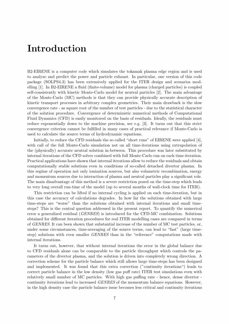
Zu beziehen durch: Forschungszentrum Jülich GmbH · Zentralbibliothek, VerlagD-52425 Jülich · Bundesrepublik DeutschlandZ 02461 61-5220 · Telefax: 02461 61-6103 · e-mail: [email protected]

Abstract

B2-EIRENE is a finite-volume Computational Fluid Dynamics (CFD) code which describesflow of magnetized charged particles combined self-consistently with kinetic Monte-Carlo (MC)model for neutral particles. The issue of the run-time and accuracy of the coupled package isaddressed in the present report. Convergence of different iteration schemes is analyzed in termsof generalized residuals. Particular focus is on the global particle balance. The results anddiscussions may be of general interest for developers and users of tokamak edge codes based ona CFD-MC combination.

B2-EIRENE ist ein Finite-Volumen Stromungsmechanik (CFD) Code der Stromungen vonmagnetisierten geladenen Teilchen beschreibt, selbst-konsistent gekoppelt mit einem kinetischenMonte-Carlo (MC) Modell fur Neutralteilchen. Der Bericht befasst sich mit dem Problem vonLaufzeit und Genauigkeit des gekoppelten Pakets. Numerische Konvergenz von verschiedeneniterativen Verfahren wird analysiert auf Grundlage von verallgemeinerten Residuen. BesonderesAugenmerk wird dabei auf globale Teilchenbilanz gelegt. Ergebnisse und Diskussion konnen vonallgemeinem Interesse sein fur Entwickler und Anwender von den auf CFD-MC Kombinationbasierten Tokamak Randschichtcodes.

3

4

Contents

Introduction 7

1 B2-EIRENE: a non-linear multi-physics problem 91.1 Mathematical model . . . . . . . . . . . . . . . . . . . . . . . . . . . . . . . . . . 91.2 Numerical procedure . . . . . . . . . . . . . . . . . . . . . . . . . . . . . . . . . . 101.3 Numerical diagnostics . . . . . . . . . . . . . . . . . . . . . . . . . . . . . . . . . 14

2 Generalized residual 152.1 General concept . . . . . . . . . . . . . . . . . . . . . . . . . . . . . . . . . . . . . 152.2 Implementation in B2-EIRENE . . . . . . . . . . . . . . . . . . . . . . . . . . . . 16

3 Time averaging of source terms 19

4 Test runs 214.1 Single fluid test . . . . . . . . . . . . . . . . . . . . . . . . . . . . . . . . . . . . . 214.2 Multi-fluid test . . . . . . . . . . . . . . . . . . . . . . . . . . . . . . . . . . . . . 26

5 The particle balance issue 315.1 Diagnostic for particle balance on the CFD side . . . . . . . . . . . . . . . . . . . 315.2 Extra iterations for correction of particle balance . . . . . . . . . . . . . . . . . . 345.3 Testing the correction scheme . . . . . . . . . . . . . . . . . . . . . . . . . . . . . 375.4 Potential problem with too strong negative sources . . . . . . . . . . . . . . . . . 385.5 Can a simplified (0D) correction be applied? . . . . . . . . . . . . . . . . . . . . . 40

6 Case studies 436.1 Tests with extra continuity iterations . . . . . . . . . . . . . . . . . . . . . . . . . 436.2 Can continuity iterations be combined with averaging? . . . . . . . . . . . . . . . 466.3 Can the time-step be increased? . . . . . . . . . . . . . . . . . . . . . . . . . . . . 486.4 A use case study . . . . . . . . . . . . . . . . . . . . . . . . . . . . . . . . . . . . 49

Summary and outlook 61

5

6 CONTENTS

.

Introduction

B2-EIRENE is a computer code which simulates the tokamak plasma edge region and is usedto analyze and predict the power and particle exhaust. In particular, one version of this codepackage (SOLPS4.3) has been extensively applied for the ITER design and scenarios mod-elling [1]. In B2-EIRENE a fluid (finite-volume) model for plasma (charged particles) is coupledself-consistently with kinetic Monte-Carlo model for neutral particles [2]. The main advantageof the Monte-Carlo (MC) methods is that they can provide physically accurate description ofkinetic transport processes in arbitrary complex geometries. Their main drawback is the slowconvergence rate - as square root of the number of test particles - due to the statistical characterof the solution procedure. Convergence of deterministic numerical methods of ComputationalFluid Dynamics (CFD) is easily monitored on the basis of residuals. Ideally, the residuals mustreduce exponentially down to the machine precision, see e.g. [3]. It turns out that this strictconvergence criterion cannot be fulfilled in many cases of practical relevance if Monte-Carlo isused to calculate the source terms of hydrodynamic equations.

Initially, to reduce the CFD residuals the so called “short runs” of EIRENE were applied [4],with call of the full Monte-Carlo simulation not on all time-iterations using extrapolation ofthe (physically) accurate neutral solution in-between. This procedure was later substituted byinternal iterations of the CFD solver combined with full Monte-Carlo run on each time-iteration.Practical applications have shown that internal iterations allow to reduce the residuals and obtaincomputationally stable solutions even in conditions of so-called detached divertor plasma. Inthis regime of operation not only ionization sources, but also volumetric recombination, energyand momentum sources due to interaction of plasma and neutral particles play a significant role.The main disadvantage of this method is a severe restriction posed on the time-step which leadsto very long overall run-time of the model (up to several months of wall-clock time for ITER).

This restriction can be lifted if no internal cycling is applied on each time-iteration, but inthis case the accuracy of calculations degrades. In how far the solutions obtained with largetime-steps are “worse” than the solutions obtained with internal iterations and small time-steps? This is the central question addressed in the present report. To quantify the numericalerror a generalized residual (GENRES) is introduced for the CFD-MC combination. Solutionsobtained for different iteration procedures for real ITER modelling cases are compared in termsof GENRES. It can been shown that substantial increase of the number of MC test particles, or,under some circumstances, time-averaging of the source terms, can lead to “fast” (large time-step) solutions with even smaller GENRES than in the “reference” computations made withinternal iterations.

It turns out, however, that without internal iterations the error in the global balance dueto CFD residuals alone can be comparable to the particle throughput which controls the pa-rameters of the divertor plasma, and the solution is driven into completely wrong direction. Acorrection scheme for the particle balance which still allows large time-steps has been designedand implemented. It was found that this extra correction (”continuity iterations“) leads tocorrect particle balance in the low density (low gas puff rate) ITER test simulations even withrelatively small number of MC particles. With high gas puffing rate - hence, dense divertor -continuity iterations lead to increased GENRES of the momentum balance equations. However,in the high density case the particle balance issue becomes less critical and continuity iterations

7

8 CONTENTS

can be can be skipped for main species.The “ITER-Julich” version of B2-EIRENE (SOLPS4.3) has been used for prototyping and

numerical tests. However, the algorithms and diagnostics described here are general and can beimplemented in any branch of B2-EIRENE (SOLPS). The outcomes and discussion can also be ofsignificance for other fusion edge codes based on CFD-MC coupling such as EDGE2D-EIRENE,SOLEDGE/EIRENE or SOLDOR/NEUT2D [5].

Chapter 1

B2-EIRENE: a non-linearmulti-physics problem

1.1 Mathematical model

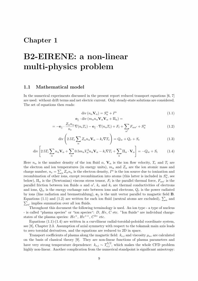
In the numerical experiments discussed in the present report reduced transport equations [6, 7]are used: without drift terms and net electric current. Only steady-state solutions are considered.The set of equations then reads:

div (nαVα) = Sαn + Iα (1.1)

e|| · div (mαnαVαVα +Πα) =

= −e|| ·Zαnαne

∇(neTe)− e|| · ∇(nαTi) + Ft +∑α′

Fαα′ + Sαu (1.2)

div

(2.5Te

∑α

ZαnαVα − ke∇Te

)= Qie +Qr + Se (1.3)

div

[2.5Ti

∑α

nαVα +∑α

0.5mαV2αnαVα − ki∇Ti +

∑α

Πα ·Vα

]= −Qie + Si (1.4)

Here nα is the number density of the ion fluid α, Vα is the ion flow velocity, Te and Ti arethe electron and ion temperatures (in energy units), mα and Zα are the ion atomic mass andcharge number, ne =

∑α Zαnα is the electron density, Iα is the ion source due to ionization and

recombination of other ions, except recombination into atoms (this latter is included in Sαn , see

below), Πα is the (Newtonian) viscous stress tensor, Ft is the parallel thermal force, Fαα‘ is theparallel friction between ion fluids α and α′, ke and ki are thermal conductivities of electronsand ions, Qie is the energy exchange rate between ions and electrons, Qr is the power radiatedby ions (line radiation and bremsstrahlung), e|| is the unit vector parallel to magnetic field B.Equations (1.1) and (1.2) are written for each ion fluid (neutral atoms are excluded),

∑α and∑

α‘ implies summation over all ion fluids.

Throughout this document the following terminology is used. An ion type - a type of nucleus- is called “plasma species” or “ion species“: D, He, C etc. ”Ion fluids“ are individual charge-states of the plasma species: He+, He++, C3+ etc.

Equations (1.1)-(1.4) are written in a curvilinear radial-toroidal-poloidal coordinate system,see [8], Chapter 2.3. Assumption of axial symmetry with respect to the tokamak main axis leadsto zero toroidal derivatives, and the equations are reduced to 2D in space.

Transport coefficients of plasma along the magnetic field: ke,i and viscosity µα, are calculatedon the basis of classical theory [9]. They are non-linear functions of plasma parameters and

have very strong temperature dependence: ke,i ∼ T5/2e,i , which makes the whole CFD problem

highly non-linear. Another complication from the numerical standpoint is significant anisotropy:

9

10 CHAPTER 1. B2-EIRENE: A NON-LINEAR MULTI-PHYSICS PROBLEM

transport coefficients in the cross-field direction are orders of magnitude smaller than the parallelones. Constant empiric cross-field coefficients are applied in the present work. Equation (1.2)is used only to find the poloidal component u of velocity Vα = e||

BBθuα + e⊥vα. Here Bθ is the

poloidal component of magnetic field. The component v perpendicular to magnetic surfaces is

calculated directly using the convection-diffusion approximation vα = −e⊥D⊥

αnα

∇nα + vconvα with

prescribed D⊥α and vconvα .

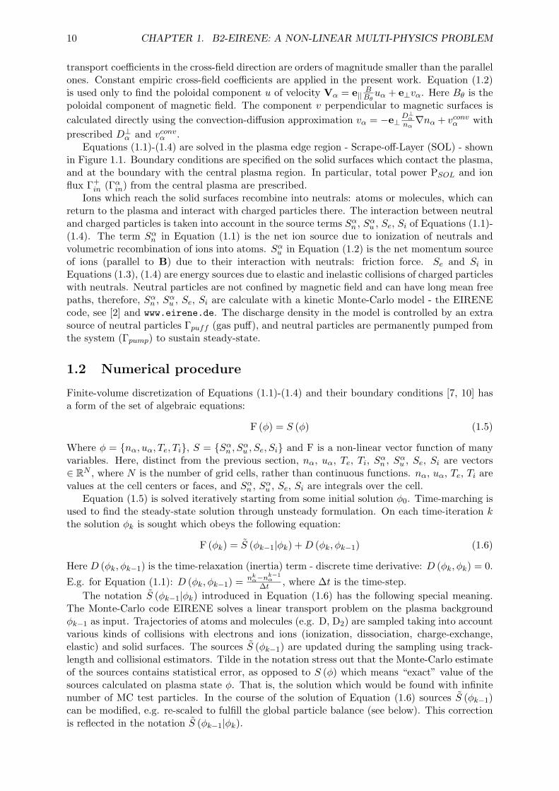
Equations (1.1)-(1.4) are solved in the plasma edge region - Scrape-off-Layer (SOL) - shownin Figure 1.1. Boundary conditions are specified on the solid surfaces which contact the plasma,and at the boundary with the central plasma region. In particular, total power PSOL and ionflux Γ+

in (Γαin) from the central plasma are prescribed.

Ions which reach the solid surfaces recombine into neutrals: atoms or molecules, which canreturn to the plasma and interact with charged particles there. The interaction between neutraland charged particles is taken into account in the source terms Sα

n , Sαu , Se, Si of Equations (1.1)-

(1.4). The term Sαn in Equation (1.1) is the net ion source due to ionization of neutrals and

volumetric recombination of ions into atoms. Sαu in Equation (1.2) is the net momentum source

of ions (parallel to B) due to their interaction with neutrals: friction force. Se and Si inEquations (1.3), (1.4) are energy sources due to elastic and inelastic collisions of charged particleswith neutrals. Neutral particles are not confined by magnetic field and can have long mean freepaths, therefore, Sα

n , Sαu , Se, Si are calculate with a kinetic Monte-Carlo model - the EIRENE

code, see [2] and www.eirene.de. The discharge density in the model is controlled by an extrasource of neutral particles Γpuff (gas puff), and neutral particles are permanently pumped fromthe system (Γpump) to sustain steady-state.

1.2 Numerical procedure

Finite-volume discretization of Equations (1.1)-(1.4) and their boundary conditions [7, 10] hasa form of the set of algebraic equations:

F (ϕ) = S (ϕ) (1.5)

Where ϕ = {nα, uα, Te, Ti}, S = {Sαn , S

αu , Se, Si} and F is a non-linear vector function of many

variables. Here, distinct from the previous section, nα, uα, Te, Ti, Sαn , S

αu , Se, Si are vectors

∈ RN , where N is the number of grid cells, rather than continuous functions. nα, uα, Te, Ti arevalues at the cell centers or faces, and Sα

n , Sαu , Se, Si are integrals over the cell.

Equation (1.5) is solved iteratively starting from some initial solution ϕ0. Time-marching isused to find the steady-state solution through unsteady formulation. On each time-iteration kthe solution ϕk is sought which obeys the following equation:

F (ϕk) = S (ϕk−1|ϕk) +D (ϕk, ϕk−1) (1.6)

Here D (ϕk, ϕk−1) is the time-relaxation (inertia) term - discrete time derivative: D (ϕk, ϕk) = 0.

E.g. for Equation (1.1): D (ϕk, ϕk−1) =nkα−nk−1

α

∆t , where ∆t is the time-step.

The notation S (ϕk−1|ϕk) introduced in Equation (1.6) has the following special meaning.The Monte-Carlo code EIRENE solves a linear transport problem on the plasma backgroundϕk−1 as input. Trajectories of atoms and molecules (e.g. D, D2) are sampled taking into accountvarious kinds of collisions with electrons and ions (ionization, dissociation, charge-exchange,elastic) and solid surfaces. The sources S (ϕk−1) are updated during the sampling using track-length and collisional estimators. Tilde in the notation stress out that the Monte-Carlo estimateof the sources contains statistical error, as opposed to S (ϕ) which means “exact” value of thesources calculated on plasma state ϕ. That is, the solution which would be found with infinitenumber of MC test particles. In the course of the solution of Equation (1.6) sources S (ϕk−1)can be modified, e.g. re-scaled to fulfill the global particle balance (see below). This correctionis reflected in the notation S (ϕk−1|ϕk).

1.2. NUMERICAL PROCEDURE 11

Γ

Γ

Γ

P

IT

pu�

in

pump

SOL

+

OT

Figure 1.1: Computational domain of B2-EIRENE for ITER: poloidal cross-section. Solid regionis SOL where Equations (1.1)-(1.4) are solved. Arrows sketch out the power flow from centralplasma to the divertor targets. IT stands for Inner Target and OT for Outer Target respectively.Bold yellow line is the magnetic separatrix.


An extra iteration loop on each time-iteration: “internal iterations”, is used to find theapproximate solution of Equation (1.6). One each internal iteration a block Gauss-Seidel schemeis applied to update the solution. That is, the fields nα, uα, Te, Ti are updated by solving oneby one equations for corrections based on the individual Equations (1.1)-(1.4). The correctionξ is calculated from the linearized form of the discretized equations as follows:

M (ϕk) ξ = S(ϕj−1k

)−M

(ϕj−1k

)ψj−1k = Rj−1

k , ψjk = ψj−1

k + rξ (1.7)

Here M (ϕ) is a matrix with coefficients dependent on ϕ, ψ is nα or uα or Te or Ti, Rj−1k is the

residual, and 0 < r ≤ 1 is the underrelaxation factor. Correction ξ is found as a solution of theset of linear equations, initial value ϕ0k = ϕmk−1 where m is the index of last internal iteration.Pseudocode of the internal iteration j+1 looks as follows (the time-iteration index k is omitted):

1. Calculating source terms and coefficients

2. Defining boundary conditions as sources in so called guard (boundary) cells

3. Momentum balance, Equation (1.2), for each α: uj+1/4α = ujα + rξ

4. Momentum balance for sum of Equations (1.2) over α:

uj+2/4α = u

j+1/4α + rξ

5. Particle balance, Equation (1.1), for each α:

nj+1/2α = njα + rξ, u

j+3/4α = u

j+2/4α − rC ∂ξ

∂x

6. Electron energy, Equation (1.3): Tj+1/2e = T j

e + rξ

7. Ion energy, Equation (1.4): Tj+1/2i = T j

i + rξ

8. Sum of Equations (1.3) and (1.4): T j+1e = T

j+1/2e + rξ, T j+1

i = Tj+1/2i + rξ

9. Repeating particle balance, Equation (1.1), for each α:

nj+1α = n

j+1/2α + rξ, uj+1

α = uj+3/4α − rC ∂ξ

∂x

Handling of momentum and continuity equations which includes velocity correction C ∂ξ∂x follows

the compressible version of the pressure correction algorithm SIMPLE by Patankar, see [10],Chapter 6.7. Its implementation in B2 is described in [7], Chapter 3. This algorithm ensurescomputational stability at both high and low Mach numbers.

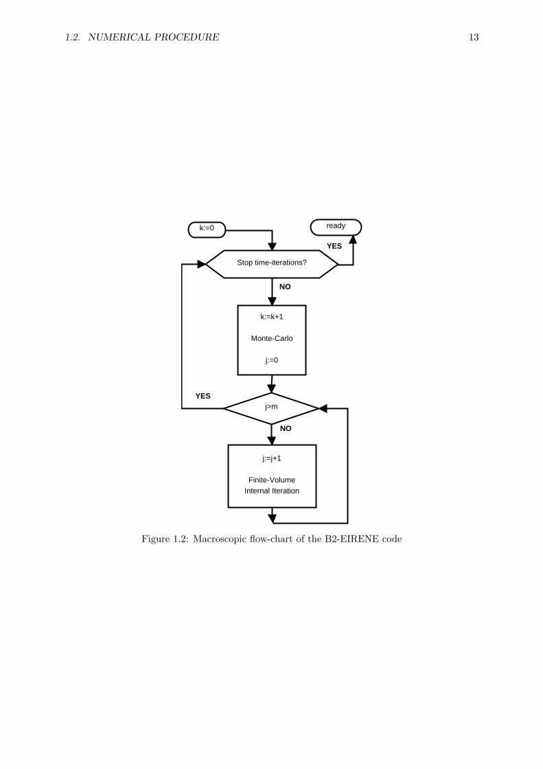
The macroscopic flow chart of the coupling between the CFD part (B2) and MC part(EIRENE) is shown in Figure 1.2. In this flow-chart a single “internal iteration” is the se-quence of steps described above.

EIRENE typically uses stratified sampling, see [11], Chapter 10.3. That is, S is calculated asa sum of contributions from Ns sources (strata) sampled independently S =

∑Nss=1 S

s. There arefour types of primary sources of neutrals in B2-EIRENE: i) recombination of ions on the solidsurfaces - recycling sources; ii) volumetric recombination of ions in plasma; iii) external gas puff;iv) sputtering from the solid surfaces. The system in question: SOL and divertor plasma, hasvery low tolerance with respect to the errors in particle balance - especially in reactor conditions,see [1]. Therefore, to avoid too strong violation of particle balance the total strength of EIRENErecycling strata has to change as the primary source - ion flux to the surfaces - changes in thecourse of internal iterations of B2. Therefore, as the solution ϕ is modified the particle sourcesare re-scaled as follows:

Sαn

(ϕ0k|ϕ

jk

)=∑s

λβs Sα,sn

(ϕ0k), λβs =

Qβs

(ϕjk

)Qβ

s

(ϕ0k) (1.8)

1.2. NUMERICAL PROCEDURE 13

k:=k+1

Monte-Carlo

j:=0

NO

YES

Stop time-iterations?

readyk:=0

j>mYES

j:=j+1

Finite-VolumeInternal Iteration

NO

Figure 1.2: Macroscopic flow-chart of the B2-EIRENE code


Here Qβs is the sink (flux) of plasma species β in B2 to which the source Sα,s

n is proportional.

E.g. if α is He+ and s is a recycling stratum, then Qβs is the total flux of He+ and He++ ions

to the plasma facing surfaces. For volumetric recombination (and gas puff) λβs is formally setto 11.

1.3 Numerical diagnostics

In the present report only steady-state solutions are considered and analyzed. Strictly speaking,the CFD-MC combination never reaches a complete steady-state because Monte-Carlo noiseand thus oscillations always remain in the solution. Here a practical definition of “steady-state”is used which is based on the estimated time-scales of selected parameters. The characteristictime-scale τX of parameter X is calculated from the time-trace X(t) by fitting it with a linearfunction:

lnX = τ−1X t+ C,

1

τX=

1

X

dX

dt

The number of last data-points used for the fit in this report is equal to max(2000, N

(5 µs)p

),

where N(5 µs)p is the number of points which cover last 5 µs of physical time. The same data-

points are used to calculate ∆Γ and ∆P below.The control parameters for which τX is calculated are the total amount of ions Nβ of species

β, total energy in the electrons Ee and ions Ei:

Nβ =

∫ ∑α′

nα′dV, Ee = 1.5

∫neTedV, Ei =

∫ (1.5∑α

nαTi + 0.5∑α

mαnαV2α

)dV

(the integration is performed over the whole B2 grid,∑

α′ is the sum over all ion fluids of speciesβ), as well as plasma parameters averaged along the magnetic separatrix: < ne >

sep, < Te >sep,

< Ti >sep.

In addition, errors in the global particle and power balance are checked. The relative errorin the steady-state particle balance for each species is written as:

∆Γ =Γpuff + Γ+

in − Γpump − Γnout

Γpuff + Γ+in

(1.9)

Here Γpuff is the (atomic) rate of gas puffing, Γ+in is the ion influx from central (core) plasma,

Γpump is the (atomic) flux absorbed on the surfaces (pumped), Γnout is the flux of atoms to the

central plasma (see Figure 1.1).The relative error in the steady-state power balance:

∆P =PSOL − P+

PFC − PnPFC − Prad − Pn

core

PSOL(1.10)

Here PSOL is the power influx to the computational domain from central plasma, P+PFC is the

power deposited by charged particles to the Plasma Facing Components (PFC) - solid surfacessurrounding the plasma, Pn

PFC is the power deposited by neutral particles to PFC, Prad is thepower radiated from plasma, Pn

core is the power transferred by neutral particles back to thecentral plasma.

1There is an option to re-scale volume recombination as well. In the tests described in this report it was foundthat in low density discharges - when volumetric recombination is weak - correction of this stratum has practicallyno effect on the resulting convergence behavior. In the tests where recombination is significant this correction wasfound to increase the error and was therefore switched off (lstrascl is set to 0 for volume recombination strata)

Chapter 2

Generalized residual

2.1 General concept

Approximate solution ϕmk can be inserted back into Equation (1.6) to calculate the residual Rmk :

Rmk = F (ϕmk )− S

(ϕ0k|ϕmk

)−D

(ϕmk , ϕ

0k

)(2.1)

Equation (2.1) can also be formally re-written as:

F (ϕmk ) = S (ϕmk ) + R, R = Rmk + S

(ϕ0k|ϕmk

)− S (ϕmk ) +D

(ϕmk , ϕ

0k

)(2.2)

That is, instead of solution ϕ∗ of Equation (1.5) the solution ϕmk of Equation (2.2) is found.Note that S (ϕmk ) is the “exact” source - as it would be calculated with infinite number of testparticles. S (ϕmk ) cannot be known in the calculations made with finite number of MC testparticles, and only an estimate of this quantity S (ϕmk ) - which contains statistical error - canbe calculated. Therefore, for R only an estimate can be found as well, but not its exact value.

It sounds plausible that ϕmk should come close to ϕ∗ if R is “small enough”. Convergence ofϕmk to ϕ∗ can be easily shown in a strict way if H (ϕ) = S (ϕ) − F (ϕ) + ϕ forms a contractivemapping. That is, for any ϕ1, ϕ2 belonging to the domain of interest:

∥H (ϕ1)−H (ϕ2)∥ ≤ δ ∥ϕ1 − ϕ2∥ (2.3)

With a parameter δ: 0 < δ < 1. Therefore, since ϕ∗ = H (ϕ∗) and ϕmk = H (ϕmk ) + R:

∥ϕ∗ − ϕmk ∥ =∥∥∥H (ϕ∗)−H (ϕmk )− R

∥∥∥ ≤ δ ∥ϕ∗ − ϕmk ∥+∥∥∥R∥∥∥⇒ ∥ϕ∗ − ϕmk ∥ ≤ 1

1− δ

∥∥∥R∥∥∥ (2.4)

That is, the distance between approximate and exact solutions is reduced when∥∥∥R∥∥∥ is re-

duced. According to the contraction mapping theorem, see [12], Chapter 5.1.3, fulfillment ofcondition (2.3) with δ < 1 is also sufficient for existence of a unique solution of Equation (1.5).

An estimate of∥∥∥R∥∥∥ can serve as a diagnostic (measure) of convergence. It is convenient to

split∥∥∥R∥∥∥ into two parts: ∥∥∥R∥∥∥ ≤ G = R+∆S (2.5)

WhereR = ∥Rm

k ∥ , ∆S =∥∥∥S (ϕ0k|ϕmk )− S (ϕmk ) +D

(ϕmk , ϕ

0k

)∥∥∥ (2.6)

G defined by Equation (2.5) is called here the generalized residual. R is the error related to theinaccuracy of solving the set of algebraic equations (1.6) - the standard CFD residual. ∆S is theerror which occurs: a) because of statustical noise and b) because the sources are calculated bythe Monte-Carlo model for “old” ϕ0k, but not for “up-to date” ϕmk . The (discrete) time derivative

15

16 CHAPTER 2. GENERALIZED RESIDUAL

is included in ∆S as well. It is to be expected that if the steady-state solution is almost reached,then both non zero D

(ϕmk , ϕ

0k

)and S

(ϕ0k|ϕmk

)− S (ϕmk ) are caused mainly by the statistical

noise in S. This is the rationale for combining those two terms in one norm.The term ∆S without time-derivative can be called the source inconsistency or operator

splitting error. With finite number of test particles exact value of ∆S is not known, and onlyits estimate can be calculated:

∆S =∥∥∥S (ϕ0k|ϕmk )− S (ϕmk ) +D

(ϕmk , ϕ

0k

)∥∥∥ (2.7)

However, with certain confidence the error E (∆S) =∣∣∣∆S −∆S

∣∣∣ can be estimated using statis-

tical methods.It is readily seen that the discussion in this section is applicable to any numerical algorithm

which can be described in the form of Equation (1.6).

2.2 Implementation in B2-EIRENE

Implementation of generalized residual, Equations (2.5), (2.6), in the B2-EIRENE code isbased on l1-norm: ∥X∥1 =

∑Ni=1 |xi|. This norm has a convenient property that if X =

{X1...Xγ ...XM}, then ∥X∥1 =∑M

γ=1 ∥Xγ∥1. Therefore, G can be split into contributions forindividual equations:

G =∑α

Gαn +

∑α

Gαu +Ge +Gi =

∑γ={α

n,αu,e,i}

Gγ , Gγ = Rγ +∆Sγ (2.8)

Where Rγ and ∆Sγ are calculated according to Equations (2.1) and (2.6) with F (ϕmk ) =

{Fγ (ϕmk )}, D

(ϕmk , ϕ

0k

)={Dγ

(ϕmk , ϕ

0k

)}, S(ϕ0k|ϕmk

)={Sγ(ϕ0k|ϕmk

)}and S (ϕmk ) = {Sγ (ϕmk )}

replaced by Fγ (ϕmk ), Dγ

(ϕmk , ϕ

0k

), Sγ

(ϕ0k|ϕmk

)and Sγ (ϕ

mk ) respectively. Indexes α

n ,αu , e, i stand

for particle, momentum, electron and ion energy balance.Equation for the generalized residual Gγ with error bars reads as follows:

Gγ = Rγ +∆Sγ +

{+3σγ

−min(3σγ ,∆Sγ

) (2.9)

Here:

σγ =

√√√√ N∑i=1

(σi (Sγ))2 (2.10)

is the mean square of the standard deviations (sample standard deviation of the mean) in the

grid cells i which approximates the standard deviation of ∆Sγ . Expression min(3σγ ,∆Sγ

)takes

into account that ∆Sγ ≥ 0. Equation (2.9) is written for confidence interval 0.997 assumingGaussian distribution of error. Equation (2.10) is strictly valid only if Sγ calculated in differentcells are completely uncorrelated. To estimate the effect of correlation the standard deviationsof ∥Sγ∥1 are also calculated and compared to Equation (2.10). For the test case ’1e-4/1/1’from Section 4.1 below the ratio between σγ calculated using Equation (2.10) and the standarddeviation of ∥Sγ∥1 is 0.77 at worst. For the case ’3e-7/20/1’ from Section 4.2 the worst caseratio is 0.43 (He momentum sources).

For practical evaluations it is more convenient to use the normalized (dimensionless) formof Gγ :

Gγ = Gγ

/∥∥∥Sγ (ϕmk )∥∥∥1

(2.11)

In the text below the normalized residual Gγ is often referred to as GENRES.

2.2. IMPLEMENTATION IN B2-EIRENE 17

Gγ should not be mixed up with errors in the particle, momentum and energy balances.Those latter are the absolute values of the sums of contributions in the individual cells - not thesums of the absolute values, and they are ≤ Gγ .

Gγ based on l1-norm can be easily further decomposed into residuals of individual regionsof the computational domain to analyze them separately.

18 CHAPTER 2. GENERALIZED RESIDUAL

Chapter 3

Time averaging of source terms

B2-EIRENE experience shows that internal iterations, m > 1, are required to reduce the residualR. However, this procedure restricts the time-step, therefore, a very large number of time-iterations is needed to reach the steady-state solution. Too large time-step can lead to divergenceof the internal iterations and hence numerical instability. With m = 1 the simulation can bestable with much larger time-steps. “Stable”, in the sense that a steady-state solution is reached.However, R, thus, GENRES are much larger in this case then those obtained with m > 1 and asmall time step. Specific examples will be discussed below in Section 5.

It turns out that R can be also significantly reduced if the source term calculated in theMonte-Carlo run S

(ϕ0k)is replaced by an average over past Lk time-iterations:

S(ϕ0k)→ Sk =

1

Lk

Lk∑l=1

S(ϕ0k−Lk+l

), Lk = mod (k − 1, L) + 1 (3.1)

That is, the averaging is restarted every L time-iterations where L is an input parameter.According to ref. [5] this particular time-averaging is applied in the code SOLDOR/NEUT2D.

It can be easily shown that the variation of Sk between two subsequent time-iterations ismuch smaller than that of the original source terms S

(ϕ0k). Indeed, if ∥Si − Sj∥ < δ, k−Lk+1 ≤

i, j ≤ k, then for Lk > 1:∥∥∥Sk − Sk−1∥∥∥ =

∥∥∥∥∥ 1

Lk

Lk∑l=1

Sl −1

Lk − 1

Lk−1∑l=1

Sl

∥∥∥∥∥ =

∥∥∥∥∥∑Lk−1

l=1 (SLk− Sl)

Lk (Lk − 1)

∥∥∥∥∥ < δ

Lk

In practice the reduction of∥∥Sk − Sk−1

∥∥ with increased Lk leads to reduction of R, an exampleis shown in Figure 4.3 below. The minimum of R is reached roughly on the time-iteration forwhich Lk = L. It makes sense, therefore, to consider the solution only on those time-iterations,and to check GENRES only on those time-iterations as well.

The error bar of the estimate of ∆S, see Equations (2.7) and (2.9), can also be significantlyreduced with moderate increase of the computational time. Increasing the number of test par-ticles when calculating S (ϕmk ) by a factor of fMC reduces the statistical error by a factor of≈

√fMC . At the same time, if the number of particles is increased only for k : Lk = L, then

the total time spent for particle sampling is increased by only a factor of (L− 1 + fMC) /L. E.g.for fMC = L/2 + 1 the accumulated Monte-Carlo time is increased by only 50 %.

To achieve better particle balance, instead of Equation (1.8) the averages of sources normal-ized to the total source strength Qγ

s for each stratum s are accumulated:

Skγ =

1

Lk

Ns∑s=1

Qsγ

(ϕ0k) Lk∑

l=1

Sγs

(ϕ0k−Lk+l

)Qs

γ

(ϕ0k−Lk+l

) (3.2)

For particle sources,γ=αn , Qγ

s is the same as Qβs in Equation (1.8). The same scaling is used for

momentum, γ=αu as well. Energy sources, γ = e, i are scaled with total ion fluxes: sum over all

19

20 CHAPTER 3. TIME AVERAGING OF SOURCE TERMS

α. Averaging described by Equation (3.2) is used in the tests described in the next section forall types of source terms: Sα

n , Sαu , Se and Si. It was found critical to use this kind of averaging

for particle sources Sαn . At the same time, for other types of sources no significant difference

between applying the Equation (3.1) or Equation (3.2) was revealed.

Chapter 4

Test runs

4.1 Single fluid test

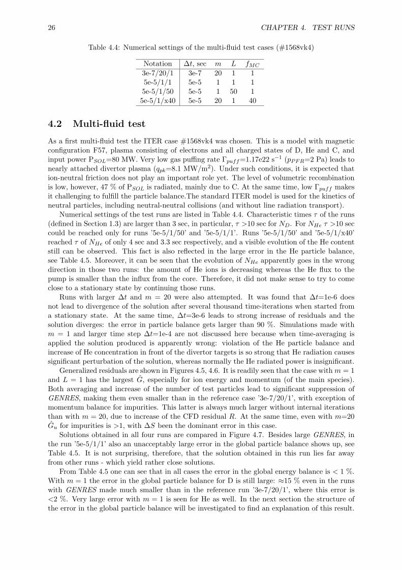
In this section different modes of operation of B2-EIRENE are analyzed in terms of generalizedresiduals. The tests are made for virtual discharge #2013vk4 from the ITER database of B2-EIRENE runs [13]. Geometry and magnetic configuration of the model is shown in Figure 1.1.D+ is the only ion species in the model plasma. Total power input from the central plasmaPSOL=38 MW. Set of atomic and molecular processes applied in the neutral transport codeis the same as that described in [14], excluding neutral-neutral collisions and opacity of lineradiation.

Intensity of interaction between neutral and charged particles in front of the divertor targets isknown to strongly depend on the neutral pressure at the the entrance to the pump duct pPFR [1].For the discharge in question pPFR=3 Pa. At such low pressure the plasma temperature in frontof the targets is relatively high: one speaks of “attached divertor”. From the point of viewof numerical solution that means relatively low importance of the momentum source Sm, andlow rate of volumetric recombination compared to recombination of ions on the plasma facingsurfaces.

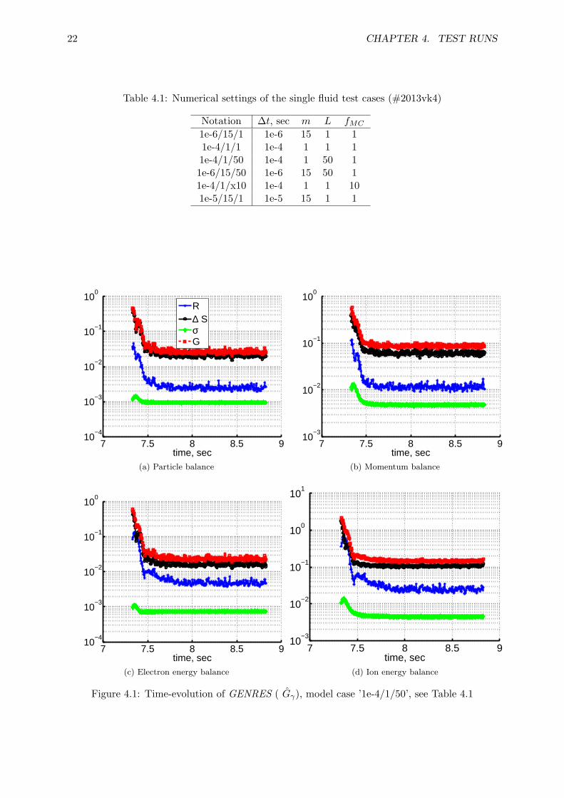
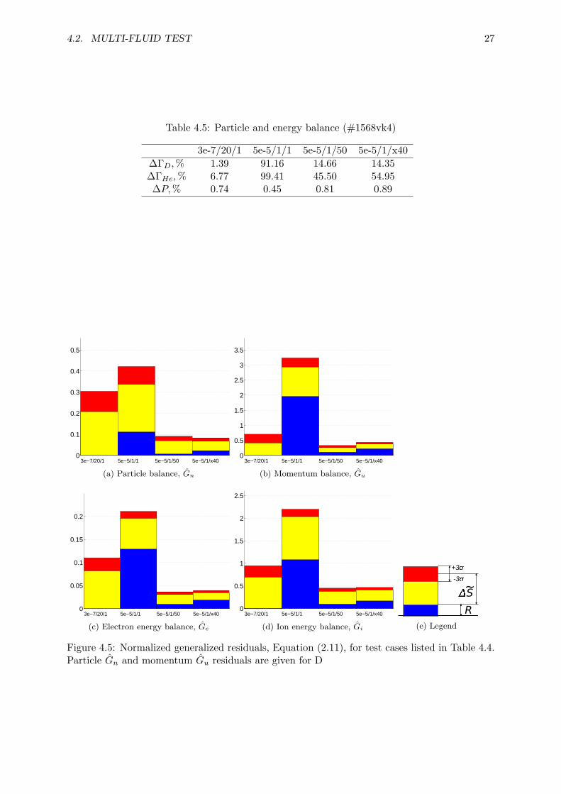
Numerical settings of the test runs are listed in Table 4.1. In this table ∆t is the timestep, m is the number of internal iterations, L is the maximum number of terms in the time-average, Equation (3.2), fMC is the multiplier for the number of test particles. All cases reachsteady-state solution with characteristic decay times τ >10 sec, see Section 1.3 for definition.

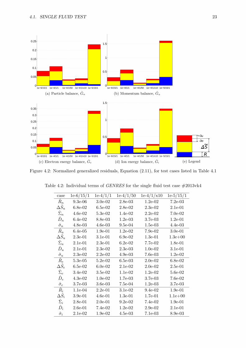
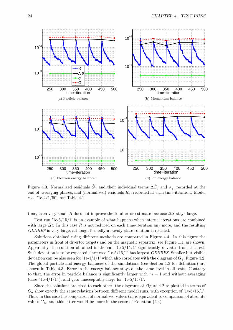
An example of the time evolution of generalized residuals is shown in Figure 4.1. The run isstarted from a non-converged initial solution. After initial perturbation the residuals saturate,and only weak oscillations remain. Diagrams of normalized generalized residuals Gγ recordedon the last time-iteration are shown in Figure 4.2. For tests with L > 1 this last iteration isthe one for which Lk = L. Numerical values of individual contributions to Gγ can be found inTable 4.2.

For simulations of ITER edge plasma the B2-EIRENE code is typically used with m > 1(m=15..20). This mode apparently ensures smallest residuals R compared to others which havebeen tried so far. With m = 1, which allows larger ∆t, the residuals Gγ are larger, mainlybecause of much larger R. Averaging, Equation (3.2), reduces both R and ∆S, making G evensmaller then that calculated with m > 1. In the runs with L > 1 the number of test-particleson the time-iterations k : Lk = L was multiplied by a factor of L/2, which is the reasonof significant reduction of σ for those cases. In the m = 1 case both R and ∆S can be alsoreduced by increasing the number of Monte-Carlo particles on each time-iteration. However, thereduction of R in this case is far less pronounced than with L > 1.

The action of averaging is demonstrated in Figure 4.3, where behavior of residuals Rγ inthe course of time-iterations is shown. Their decrease on the time averaging phase is clearlyseen. Although averaging helps to significantly decrease Rγ , those residuals are still orders ofmagnitude larger than what can be achieved with internal iterations, see Table 4.2. At the same

21

22 CHAPTER 4. TEST RUNS

Table 4.1: Numerical settings of the single fluid test cases (#2013vk4)

Notation ∆t, sec m L fMC

1e-6/15/1 1e-6 15 1 11e-4/1/1 1e-4 1 1 11e-4/1/50 1e-4 1 50 11e-6/15/50 1e-6 15 50 11e-4/1/x10 1e-4 1 1 101e-5/15/1 1e-5 15 1 1

7 7.5 8 8.5 910

−4

10−3

10−2

10−1

100

time, sec

R∆ SσG

(a) Particle balance

7 7.5 8 8.5 910

−3

10−2

10−1

100

time, sec

(b) Momentum balance

7 7.5 8 8.5 910

−4

10−3

10−2

10−1

100

time, sec

(c) Electron energy balance

7 7.5 8 8.5 910

−3

10−2

10−1

100

101

time, sec(d) Ion energy balance

Figure 4.1: Time-evolution of GENRES ( Gγ), model case ’1e-4/1/50’, see Table 4.1

4.1. SINGLE FLUID TEST 23

0

0.05

0.1

0.15

0.2

0.25

1e−6/15/1 1e−4/1/1 1e−4/1/50 1e−4/1/x10 1e−5/15/1

(a) Particle balance, Gn

0

0.5

1

1.5

1e−6/15/1 1e−4/1/1 1e−4/1/50 1e−4/1/x10 1e−5/15/1

(b) Momentum balance, Gu

0

0.05

0.1

0.15

0.2

0.25

0.3

0.35

1e−6/15/1 1e−4/1/1 1e−4/1/50 1e−4/1/x10 1e−5/15/1

(c) Electron energy balance, Ge

0

0.5

1

1.5

1e−6/15/1 1e−4/1/1 1e−4/1/50 1e−4/1/x10 1e−5/15/1

(d) Ion energy balance, Gi

R

S

+3�

-3�

~

(e) Legend

Figure 4.2: Normalized generalized residuals, Equation (2.11), for test cases listed in Table 4.1

Table 4.2: Individual terms of GENRES for the single fluid test case #2013vk4

case 1e-6/15/1 1e-4/1/1 1e-4/1/50 1e-4/1/x10 1e-5/15/1

Rn 9.3e-06 3.0e-02 2.8e-03 1.2e-02 7.2e-03

∆Sn 6.8e-02 6.5e-02 2.8e-02 2.3e-02 2.1e-01

Σn 4.6e-02 5.3e-02 1.4e-02 2.2e-02 7.0e-02

Dn 6.4e-02 8.8e-03 1.2e-03 3.7e-03 1.2e-01σn 4.8e-03 4.6e-03 9.5e-04 1.5e-03 4.4e-03

Ru 6.4e-05 1.9e-01 1.2e-02 7.9e-02 3.0e-01

∆Su 2.3e-01 3.1e-01 6.9e-02 1.3e-01 1.3e+00

Σu 2.1e-01 2.3e-01 6.2e-02 7.7e-02 1.8e-01

Du 2.1e-01 2.3e-02 2.3e-03 1.0e-02 3.1e-01σu 2.3e-02 2.2e-02 4.9e-03 7.6e-03 1.2e-02

Re 5.3e-05 5.2e-02 6.5e-03 2.0e-02 6.8e-02

∆Se 6.5e-02 6.0e-02 2.1e-02 2.0e-02 2.5e-01

Σe 3.4e-02 3.5e-02 1.1e-02 1.2e-02 5.6e-02

De 4.3e-02 1.0e-02 1.7e-03 3.7e-03 7.6e-02σe 3.7e-03 3.6e-03 7.5e-04 1.2e-03 3.7e-03

Ri 1.1e-04 2.2e-01 3.1e-02 9.4e-02 1.9e-01

∆Si 3.9e-01 4.6e-01 1.3e-01 1.7e-01 1.1e+00

Σi 2.8e-01 2.0e-01 9.2e-02 7.4e-02 1.9e-01

Di 2.6e-01 7.4e-02 1.2e-02 2.9e-02 2.1e-01σi 2.1e-02 1.9e-02 4.5e-03 7.1e-03 8.9e-03


250 300 350 400 450 500

10−3

10−2

time−iteration

R∆ SσG

(a) Particle balance

250 300 350 400 450 500

10−2

10−1

time−iteration

(b) Momentum balance

250 300 350 400 450 500

10−3

10−2

time−iteration


250 300 350 400 450 500

10−2

10−1

time−iteration(d) Ion energy balance

Figure 4.3: Normalized residuals Gγ and their individual terms ∆Sγ and σγ , recorded at theend of averaging phases, and (normalized) residuals Rγ , recorded at each time-iteration. Modelcase ’1e-4/1/50’, see Table 4.1

time, even very small R does not improve the total error estimate because ∆S stays large.

Test run ’1e-5/15/1’ is an example of what happens when internal iterations are combinedwith large ∆t. In this case R is not reduced on each time-iteration any more, and the resultingGENRES is very large, although formally a steady-state solution is reached.

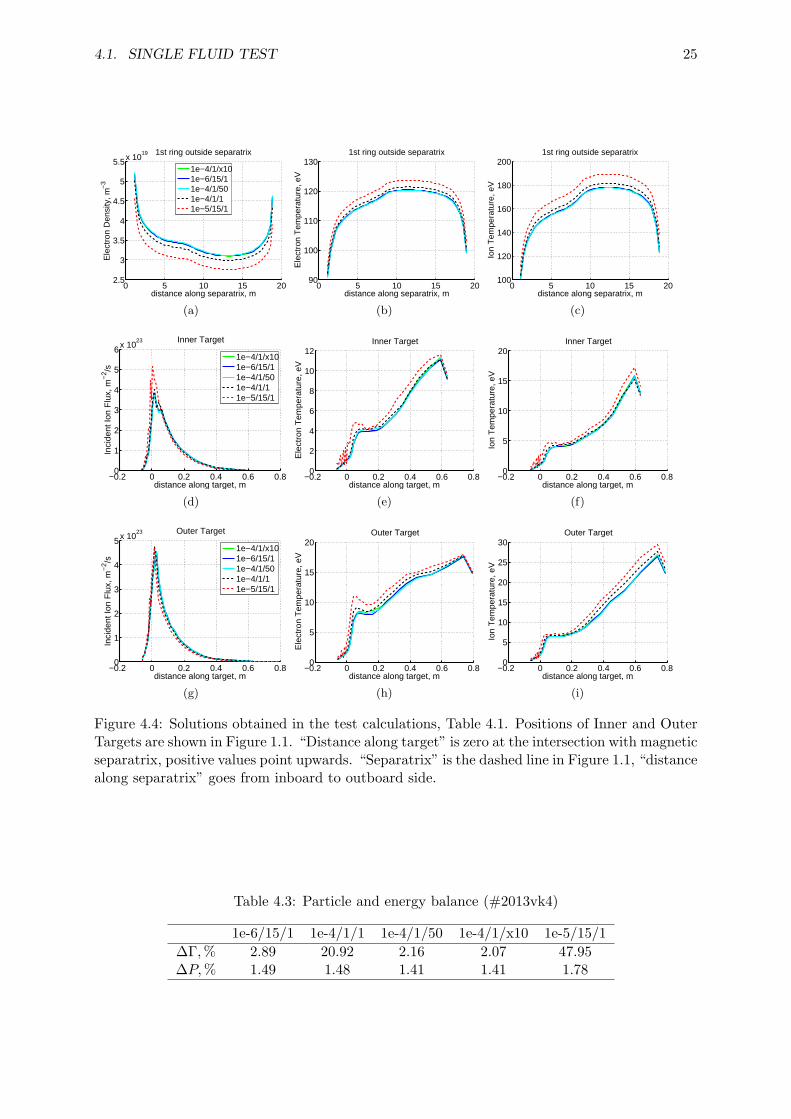
Solutions obtained using different methods are compared in Figure 4.4. In this figure theparameters in front of divertor targets and on the magnetic separtrix, see Figure 1.1, are shown.Apparently, the solution obtained in the run ’1e-5/15/1’ significantly deviates from the rest.Such deviation is to be expected since case ’1e-5/15/1’ has largest GENRES. Smaller but visibledeviation can be also seen for ’1e-4/1/1’ which also correlates with the diagram of Gγ , Figure 4.2.The global particle and energy balances of the simulations (see Section 1.3 for definition) areshown in Table 4.3. Error in the energy balance stays on the same level in all tests. Contraryto that, the error in particle balance is significantly larger with m = 1 and without averaging(case “1e-4/1/1”), and gets unacceptably large for ’1e-5/15/1’.

Since the solutions are close to each other, the diagrams of Figure 4.2 re-plotted in terms ofGα show exactly the same relations between different model runs, with exception of ’1e-5/15/1’.Thus, in this case the comparison of normalized values Gα is equivalent to comparison of absolutevalues Gα, and this latter would be more in the sense of Equation (2.4).

4.1. SINGLE FLUID TEST 25

0 5 10 15 202.5

3

3.5

4

4.5

5

5.5x 1019 1st ring outside separatrix

distance along separatrix, m

Ele

ctro

n D

ensi

ty, m

−3

1e−4/1/x101e−6/15/11e−4/1/501e−4/1/11e−5/15/1

(a)

0 5 10 15 2090

100

110

120

1301st ring outside separatrix

distance along separatrix, mE

lect

ron

Tem

pera

ture

, eV

(b)

0 5 10 15 20100

120

140

160

180



Ion

Tem

pera

ture

, eV

(c)

−0.2 0 0.2 0.4 0.6 0.80

1

2

3

4

5

6x 1023 Inner Target

distance along target, m

Inci

dent

Ion

Flu

x, m

−2 /s

1e−4/1/x101e−6/15/11e−4/1/501e−4/1/11e−5/15/1

(d)

−0.2 0 0.2 0.4 0.6 0.80

2

4

6

8

10

12Inner Target


Ele

ctro

n T

empe

ratu

re, e

V

(e)

−0.2 0 0.2 0.4 0.6 0.80

5

10

15

20Inner Target

distance along target, mIo

n T

empe

ratu

re, e

V

(f)

−0.2 0 0.2 0.4 0.6 0.80

1

2

3

4

5x 1023 Outer Target


Inci

dent

Ion

Flu

x, m

−2 /s

1e−4/1/x101e−6/15/11e−4/1/501e−4/1/11e−5/15/1

(g)

−0.2 0 0.2 0.4 0.6 0.80

5

10

15

20Outer Target


Ele

ctro

n T

empe

ratu

re, e

V

(h)

−0.2 0 0.2 0.4 0.6 0.80

5

10

15

20

25

30Outer Target


Ion

Tem

pera

ture

, eV

(i)

Figure 4.4: Solutions obtained in the test calculations, Table 4.1. Positions of Inner and OuterTargets are shown in Figure 1.1. “Distance along target” is zero at the intersection with magneticseparatrix, positive values point upwards. “Separatrix” is the dashed line in Figure 1.1, “distancealong separatrix” goes from inboard to outboard side.

Table 4.3: Particle and energy balance (#2013vk4)

1e-6/15/1 1e-4/1/1 1e-4/1/50 1e-4/1/x10 1e-5/15/1

∆Γ,% 2.89 20.92 2.16 2.07 47.95∆P,% 1.49 1.48 1.41 1.41 1.78


Table 4.4: Numerical settings of the multi-fluid test cases (#1568vk4)

Notation ∆t, sec m L fMC

3e-7/20/1 3e-7 20 1 15e-5/1/1 5e-5 1 1 15e-5/1/50 5e-5 1 50 15e-5/1/x40 5e-5 20 1 40

4.2 Multi-fluid test

As a first multi-fluid test the ITER case #1568vk4 was chosen. This is a model with magneticconfiguration F57, plasma consisting of electrons and all charged states of D, He and C, andinput power PSOL=80 MW. Very low gas puffing rate Γpuff=1.17e22 s−1 (pPFR=2 Pa) leads tonearly attached divertor plasma (qpk=8.1 MW/m2). Under such conditions, it is expected thation-neutral friction does not play an important role yet. The level of volumetric recombinationis low, however, 47 % of PSOL is radiated, mainly due to C. At the same time, low Γpuff makesit challenging to fulfill the particle balance.The standard ITER model is used for the kinetics ofneutral particles, including neutral-neutral collisions (and without line radiation transport).

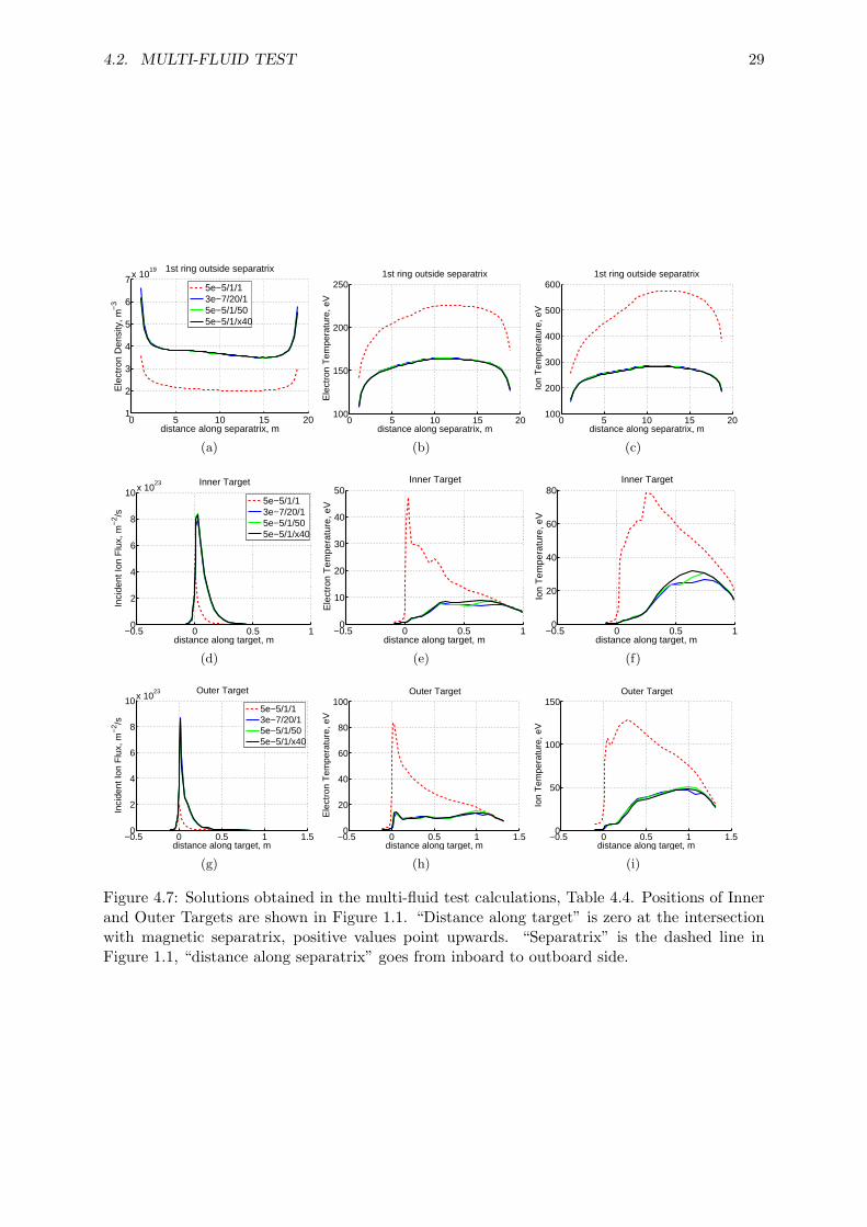
Numerical settings of the test runs are listed in Table 4.4. Characteristic times τ of the runs(defined in Section 1.3) are larger than 3 sec, in particular, τ >10 sec for ND. For NHe τ >10 seccould be reached only for runs ’5e-5/1/50’ and ’5e-5/1/1’. Runs ’5e-5/1/50’ and ’5e-5/1/x40’reached τ of NHe of only 4 sec and 3.3 sec respectively, and a visible evolution of the He contentstill can be observed. This fact is also reflected in the large error in the He particle balance,see Table 4.5. Moreover, it can be seen that the evolution of NHe apparently goes in the wrongdirection in those two runs: the amount of He ions is decreasing whereas the He flux to thepump is smaller than the influx from the core. Therefore, it did not make sense to try to comeclose to a stationary state by continuing those runs.

Runs with larger ∆t and m = 20 were also attempted. It was found that ∆t=1e-6 doesnot lead to divergence of the solution after several thousand time-iterations when started froma stationary state. At the same time, ∆t=3e-6 leads to strong increase of residuals and thesolution diverges: the error in particle balance gets larger than 90 %. Simulations made withm = 1 and larger time step ∆t=1e-4 are not discussed here because when time-averaging isapplied the solution produced is apparently wrong: violation of the He particle balance andincrease of He concentration in front of the divertor targets is so strong that He radiation causessignificant perturbation of the solution, whereas normally the He radiated power is insignificant.

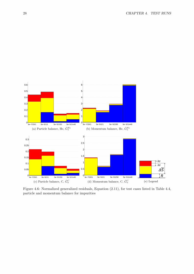
Generalized residuals are shown in Figures 4.5, 4.6. It is readily seen that the case withm = 1and L = 1 has the largest G, especially for ion energy and momentum (of the main species).Both averaging and increase of the number of test particles lead to significant suppression ofGENRES, making them even smaller than in the reference case ’3e-7/20/1’, with exception ofmomentum balance for impurities. This latter is always much larger without internal iterationsthan with m = 20, due to increase of the CFD residual R. At the same time, even with m=20Gu for impurities is >1, with ∆S been the dominant error in this case.

Solutions obtained in all four runs are compared in Figure 4.7. Besides large GENRES, inthe run ’5e-5/1/1’ also an unacceptably large error in the global particle balance shows up, seeTable 4.5. It is not surprising, therefore, that the solution obtained in this run lies far awayfrom other runs - which yield rather close solutions.

From Table 4.5 one can see that in all cases the error in the global energy balance is < 1 %.With m = 1 the error in the global particle balance for D is still large: ≈15 % even in the runswith GENRES made much smaller than in the reference run ’3e-7/20/1’, where this error is<2 %. Very large error with m = 1 is seen for He as well. In the next section the structure ofthe error in the global particle balance will be investigated to find an explanation of this result.

4.2. MULTI-FLUID TEST 27


3e-7/20/1 5e-5/1/1 5e-5/1/50 5e-5/1/x40

∆ΓD,% 1.39 91.16 14.66 14.35∆ΓHe,% 6.77 99.41 45.50 54.95∆P,% 0.74 0.45 0.81 0.89

0

0.1

0.2

0.3

0.4

0.5

3e−7/20/1 5e−5/1/1 5e−5/1/50 5e−5/1/x40


0

0.5

1

1.5

2

2.5

3

3.5

3e−7/20/1 5e−5/1/1 5e−5/1/50 5e−5/1/x40


0

0.05

0.1

0.15

0.2

3e−7/20/1 5e−5/1/1 5e−5/1/50 5e−5/1/x40


0

0.5

1

1.5

2

2.5

3e−7/20/1 5e−5/1/1 5e−5/1/50 5e−5/1/x40


R

S

+3�

-3�

~

(e) Legend

Figure 4.5: Normalized generalized residuals, Equation (2.11), for test cases listed in Table 4.4.Particle Gn and momentum Gu residuals are given for D


0

0.1

0.2

0.3

0.4

0.5

0.6

3e−7/20/1 5e−5/1/1 5e−5/1/50 5e−5/1/x40

(a) Particle balance, He, GHen

0

1

2

3

4

5

6

3e−7/20/1 5e−5/1/1 5e−5/1/50 5e−5/1/x40

(b) Momentum balance, He, GHeu

0

0.05

0.1

0.15

0.2

0.25

0.3

3e−7/20/1 5e−5/1/1 5e−5/1/50 5e−5/1/x40

(c) Particle balance, C, GCn

0

0.5

1

1.5

2

2.5

3

3e−7/20/1 5e−5/1/1 5e−5/1/50 5e−5/1/x40

(d) Momentum balance, C, GCu

R

S

+3�

-3�

~

(e) Legend

Figure 4.6: Normalized generalized residuals, Equation (2.11), for test cases listed in Table 4.4,particle and momentum balance for impurities

4.2. MULTI-FLUID TEST 29

0 5 10 15 201

2

3

4

5

6

7x 1019 1st ring outside separatrix


Ele

ctro

n D

ensi

ty, m

−3

5e−5/1/13e−7/20/15e−5/1/505e−5/1/x40

(a)

0 5 10 15 20100

150

200



Ele

ctro

n T

empe

ratu

re, e

V

(b)

0 5 10 15 20100

200

300

400

500



Ion

Tem

pera

ture

, eV

(c)

−0.5 0 0.5 10

2

4

6

8



Inci

dent

Ion

Flu

x, m

−2 /s

5e−5/1/13e−7/20/15e−5/1/505e−5/1/x40

(d)

−0.5 0 0.5 10

10

20

30

40

50Inner Target


Ele

ctro

n T

empe

ratu

re, e

V

(e)

−0.5 0 0.5 10

20

40

60

80Inner Target


Ion

Tem

pera

ture

, eV

(f)

−0.5 0 0.5 1 1.50

2

4

6

8



Inci

dent

Ion

Flu

x, m

−2 /s

5e−5/1/13e−7/20/15e−5/1/505e−5/1/x40

(g)

−0.5 0 0.5 1 1.50

20

40

60

80

100Outer Target


Ele

ctro

n T

empe

ratu

re, e

V

(h)

−0.5 0 0.5 1 1.50

50

100

150Outer Target


Ion

Tem

pera

ture

, eV

(i)

Figure 4.7: Solutions obtained in the multi-fluid test calculations, Table 4.4. Positions of Innerand Outer Targets are shown in Figure 1.1. “Distance along target” is zero at the intersectionwith magnetic separatrix, positive values point upwards. “Separatrix” is the dashed line inFigure 1.1, “distance along separatrix” goes from inboard to outboard side.


Chapter 5

The particle balance issue

5.1 Diagnostic for particle balance on the CFD side

The expression for the error in the global particle balance for the ion fluid α can be derived inthe same way as Equation (2.2) for generalized residual:

Rαn = Rα

n (m, k) + Sαn

(ϕ0k|ϕmk

)− Sα

n (ϕmk ) +Dαn

(ϕmk , ϕ

0k

)(5.1)

In this equation, as opposed to Equation (2.2), Sαn (ϕmk ) is used instead of Sα

n (ϕmk ) because theerror in the balance shows inconsistency between the actual sources and sinks in the model -independent of the error in the source and sink themselves. The global (integrated) error is thencalculated for each ion species β as:

Eβ =∑α′

∑i

(Rα′

n (m, k) + Sα′n

(ϕ0k|ϕmk

)− Sα′

n (ϕmk ) +Dα′n

(ϕmk , ϕ

0k

))Here the sum is taken over all grid cells i and over ion fluids α′ which belong to the ion speciesβ: e.g. for the He species these are ion fluids He+ and He++. The error can be presented as asum of three terms:

Eβ = EβR + Eβ

∆ + EβT (5.2)

EβR is the error due to CFD (B2) residual:

EβR =

∑α′

∑i

Rα′n (m, k)

Eβ∆ is the inconsistency of sources at the beginning and at the end of the time-iteration:

Eβ∆ =

∑α′

∑i

(Sα‘n

(ϕ0k|ϕmk

)− Sα′

n (ϕmk ))

EβT is the time-derivative:

EβT =

∑α‘

∑i

Dα‘n

(ϕmk , ϕ

0k

)The time-derivative term Eβ

T is, strictly speaking, not an error, but is considered as “error” inthe steady-state solution.

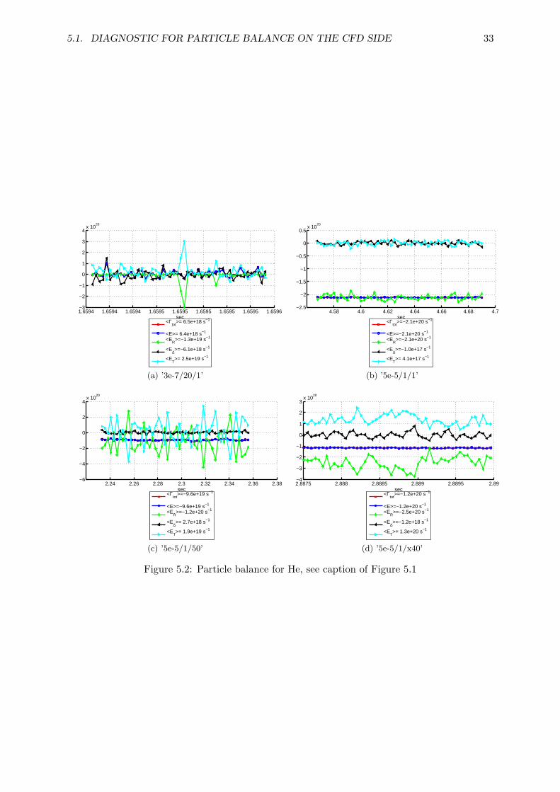
Terms of Equation (5.2) are plotted in Figures 5.1 and 5.2 for modelling runs of Section 4.2.50 last recorded data-points are shown. The new diagnostic, Equation (5.2), is compared to thestandard B2 diagnostic based on fluxes, Equation (1.9). This latter contains a slight inconsis-tency: Γpump and Γn

out on the time-iteration k are not taken from the Monte-Carlo run on thebackground plasma ϕmk . Instead, they are extrapolated from the MC run on plasma ϕ0k using

31

32 CHAPTER 5. THE PARTICLE BALANCE ISSUE

1.6594 1.6594 1.6594 1.6595 1.6595 1.6595 1.6595 1.6595 1.6596−1

−0.5

0

0.5

1x 10

22

sec

<Γtot

>=−4.3e+20 s−1

<E>=−4.5e+20 s−1

<ER>=−5.5e+18 s−1

<E∆>=−1.4e+20 s−1

<ET>=−3.1e+20 s−1

(a) ’3e-7/20/1’

4.58 4.6 4.62 4.64 4.66 4.68 4.7−4

−3

−2

−1

0

1

2x 10

22

sec

<Γtot

>=−1.9e+22 s−1

<E>=−1.9e+22 s−1

<ER>=−2.0e+22 s−1

<E∆>=−1.8e+20 s−1

<ET>= 7.6e+20 s−1

(b) ’5e-5/1/1’

2.24 2.26 2.28 2.3 2.32 2.34 2.36 2.38−1.5

−1

−0.5

0

0.5

1x 10

22

sec

<Γtot

>=−2.9e+21 s−1

<E>=−2.9e+21 s−1

<ER>=−2.0e+21 s−1

<E∆>= 1.5e+20 s−1

<ET>=−9.9e+20 s−1

(c) ’5e-5/1/50’

2.8875 2.888 2.8885 2.889 2.8895 2.89−1.5

−1

−0.5

0

0.5

1x 10

22

sec

<Γtot

>=−3.0e+21 s−1

<E>=−3.0e+21 s−1

<ER>=−2.7e+21 s−1

<E∆>=−2.3e+20 s−1

<ET>=−3.6e+19 s−1

(d) ’5e-5/1/x40’

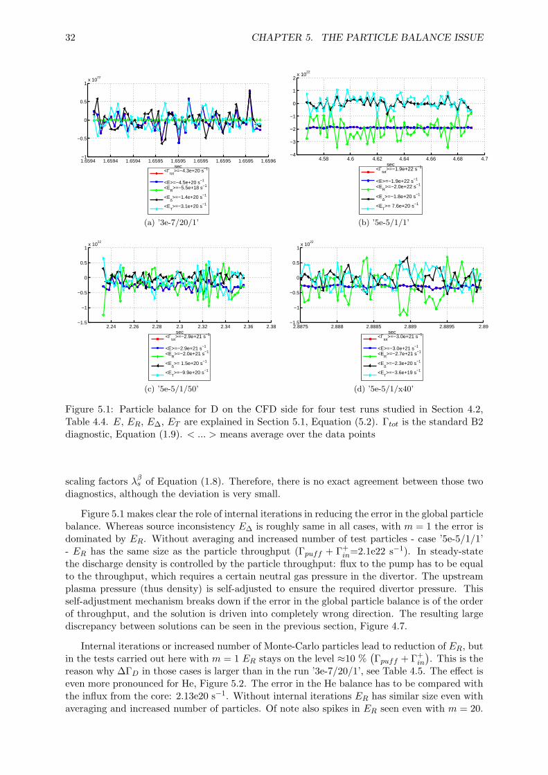
Figure 5.1: Particle balance for D on the CFD side for four test runs studied in Section 4.2,Table 4.4. E, ER, E∆, ET are explained in Section 5.1, Equation (5.2). Γtot is the standard B2diagnostic, Equation (1.9). < ... > means average over the data points

scaling factors λβs of Equation (1.8). Therefore, there is no exact agreement between those twodiagnostics, although the deviation is very small.

Figure 5.1 makes clear the role of internal iterations in reducing the error in the global particlebalance. Whereas source inconsistency E∆ is roughly same in all cases, with m = 1 the error isdominated by ER. Without averaging and increased number of test particles - case ’5e-5/1/1’- ER has the same size as the particle throughput (Γpuff + Γ+

in=2.1e22 s−1). In steady-statethe discharge density is controlled by the particle throughput: flux to the pump has to be equalto the throughput, which requires a certain neutral gas pressure in the divertor. The upstreamplasma pressure (thus density) is self-adjusted to ensure the required divertor pressure. Thisself-adjustment mechanism breaks down if the error in the global particle balance is of the orderof throughput, and the solution is driven into completely wrong direction. The resulting largediscrepancy between solutions can be seen in the previous section, Figure 4.7.

Internal iterations or increased number of Monte-Carlo particles lead to reduction of ER, butin the tests carried out here with m = 1 ER stays on the level ≈10 %

(Γpuff + Γ+

in

). This is the

reason why ∆ΓD in those cases is larger than in the run ’3e-7/20/1’, see Table 4.5. The effect iseven more pronounced for He, Figure 5.2. The error in the He balance has to be compared withthe influx from the core: 2.13e20 s−1. Without internal iterations ER has similar size even withaveraging and increased number of particles. Of note also spikes in ER seen even with m = 20.

5.1. DIAGNOSTIC FOR PARTICLE BALANCE ON THE CFD SIDE 33

1.6594 1.6594 1.6594 1.6595 1.6595 1.6595 1.6595 1.6595 1.6596−3

−2

−1

0

1

2

3

4x 10

20

sec

<Γtot

>= 6.5e+18 s−1

<E>= 6.4e+18 s−1

<ER>=−1.3e+19 s−1

<E∆>=−6.1e+18 s−1

<ET>= 2.5e+19 s−1

(a) ’3e-7/20/1’

4.58 4.6 4.62 4.64 4.66 4.68 4.7−2.5

−2

−1.5

−1

−0.5

0

0.5x 10

20

sec

<Γtot

>=−2.1e+20 s−1

<E>=−2.1e+20 s−1

<ER>=−2.1e+20 s−1

<E∆>=−1.0e+17 s−1

<ET>= 4.1e+17 s−1

(b) ’5e-5/1/1’

2.24 2.26 2.28 2.3 2.32 2.34 2.36 2.38−6

−4

−2

0

2

4x 10

20

sec

<Γtot

>=−9.6e+19 s−1

<E>=−9.6e+19 s−1

<ER>=−1.2e+20 s−1

<E∆>= 2.7e+18 s−1

<ET>= 1.9e+19 s−1

(c) ’5e-5/1/50’

2.8875 2.888 2.8885 2.889 2.8895 2.89−4

−3

−2

−1

0

1

2

3x 10

20

sec

<Γtot

>=−1.2e+20 s−1

<E>=−1.2e+20 s−1

<ER>=−2.5e+20 s−1

<E∆>=−1.2e+18 s−1

<ET>= 1.3e+20 s−1

(d) ’5e-5/1/x40’

Figure 5.2: Particle balance for He, see caption of Figure 5.1


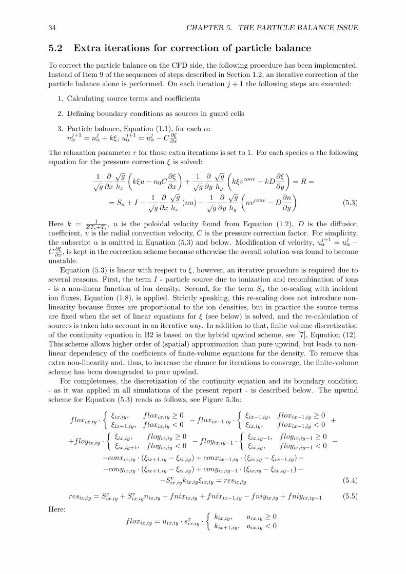
5.2 Extra iterations for correction of particle balance

To correct the particle balance on the CFD side, the following procedure has been implemented.Instead of Item 9 of the sequences of steps described in Section 1.2, an iterative correction of theparticle balance alone is performed. On each iteration j + 1 the following steps are executed:

1. Calculating source terms and coefficients

2. Defining boundary conditions as sources in guard cells

3. Particle balance, Equation (1.1), for each α:nj+1α = njα + kξ, uj+1

α = ujα − C ∂ξ∂x

The relaxation parameter r for those extra iterations is set to 1. For each species α the followingequation for the pressure correction ξ is solved:

1√g

∂

∂x

√g

hx

(kξu− n0C

∂ξ

∂x

)+

1√g

∂

∂y

√g

hy

(kξvconv − kD

∂ξ

∂y

)= R =

= Sn + I − 1√g

∂

∂x

√g

hx(nu)− 1

√g

∂

∂y

√g

hy

(nvconv −D

∂n

∂y

)(5.3)

Here k = 1ZTe+Ti

, u is the poloidal velocity found from Equation (1.2), D is the diffusioncoefficient, v is the radial convection velocity, C is the pressure correction factor. For simplicity,the subscript α is omitted in Equation (5.3) and below. Modification of velocity, uj+1

α = ujα −C ∂ξ

∂x , is kept in the correction scheme because otherwise the overall solution was found to becomeunstable.

Equation (5.3) is linear with respect to ξ, however, an iterative procedure is required due toseveral reasons. First, the term I - particle source due to ionization and recombination of ionsis a non-linear function of ion density. Second, for the term Sn the re-scaling with incidention fluxes, Equation (1.8), is applied. Strictly speaking, this re-scaling does not introduce non-linearity because fluxes are proportional to the ion densities, but in practice the source termsare fixed when the set of linear equations for ξ (see below) is solved, and the re-calculation ofsources is taken into account in an iterative way. In addition to that, finite volume discretizationof the continuity equation in B2 is based on the hybrid upwind scheme, see [7], Equation (12).This scheme allows higher order of (spatial) approximation than pure upwind, but leads to non-linear dependency of the coefficients of finite-volume equations for the density. To remove thisextra non-linearity and, thus, to increase the chance for iterations to converge, the finite-volumescheme has been downgraded to pure upwind.

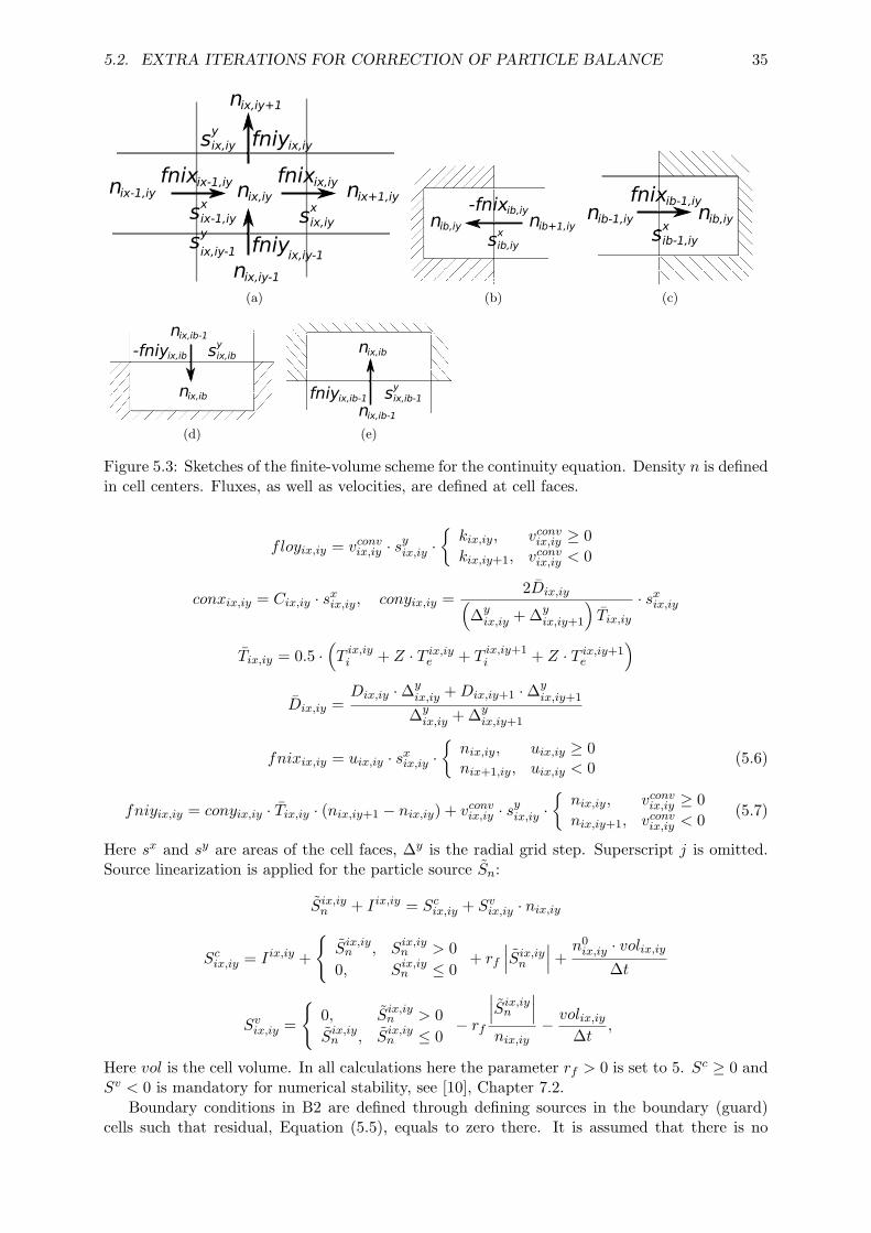
For completeness, the discretization of the continuity equation and its boundary condition- as it was applied in all simulations of the present report - is described below. The upwindscheme for Equation (5.3) reads as follows, see Figure 5.3a:

floxix,iy ·{ξix,iy, f loxix,iy ≥ 0ξix+1,iy, f loxix,iy < 0

− floxix−1,iy ·{ξix−1,iy, f loxix−1,iy ≥ 0ξix,iy, f loxix−1,iy < 0

+

+floyix,iy ·{ξix,iy, f loyix,iy ≥ 0ξix,iy+1, f loyix,iy < 0

− floyix,iy−1 ·{ξix,iy−1, f loyix,iy−1 ≥ 0ξix,iy, f loyix,iy−1 < 0

−

−conxix,iy · (ξix+1,iy − ξix,iy) + conxix−1,iy · (ξix,iy − ξix−1,iy)−−conyix,iy · (ξix+1,iy − ξix,iy) + conyix,iy−1 · (ξix,iy − ξix,iy−1)−

−Svix,iykix,iyξix,iy = resix,iy (5.4)

resix,iy = Scix,iy + Sv

ix,iynix,iy − fnixix,iy + fnixix−1,iy − fniyix,iy + fniyix,iy−1 (5.5)

Here:

floxix,iy = uix,iy · sxix,iy ·{kix,iy, uix,iy ≥ 0kix+1,iy, uix,iy < 0

5.2. EXTRA ITERATIONS FOR CORRECTION OF PARTICLE BALANCE 35

ix,iy

ix,iy-1

ix,iy+1n

n

n

ix+1,iynix-1,iyn ix-1,iyfnix

ix-1,iysx

ix,iyfnix

ix,iysx

ix,iyfniyix,iysy

ix,iy-1fniyix,iy-1

sy

(a)

ib+1,iynib,iynib,iy-fnix

ib,iysx

(b)

ib-1,iyn ib,iynib-1,iyfnix

ib-1,iysx

(c)

ix,ib-1n

ix,ibn

ix,ib-fniy ix,ibsy

(d)

ix,ibn

ix,ib-1nix,ib-1fniy ix,ib-1s

y

(e)

Figure 5.3: Sketches of the finite-volume scheme for the continuity equation. Density n is definedin cell centers. Fluxes, as well as velocities, are defined at cell faces.

floyix,iy = vconvix,iy · syix,iy ·

{kix,iy, vconvix,iy ≥ 0

kix,iy+1, vconvix,iy < 0

conxix,iy = Cix,iy · sxix,iy, conyix,iy =2Dix,iy(

∆yix,iy +∆y

ix,iy+1

)Tix,iy

· sxix,iy

Tix,iy = 0.5 ·(T ix,iyi + Z · T ix,iy

e + T ix,iy+1i + Z · T ix,iy+1

e

)Dix,iy =

Dix,iy ·∆yix,iy +Dix,iy+1 ·∆y

ix,iy+1

∆yix,iy +∆y

ix,iy+1

fnixix,iy = uix,iy · sxix,iy ·{nix,iy, uix,iy ≥ 0nix+1,iy, uix,iy < 0

(5.6)

fniyix,iy = conyix,iy · Tix,iy · (nix,iy+1 − nix,iy) + vconvix,iy · syix,iy ·

{nix,iy, vconvix,iy ≥ 0

nix,iy+1, vconvix,iy < 0(5.7)

Here sx and sy are areas of the cell faces, ∆y is the radial grid step. Superscript j is omitted.Source linearization is applied for the particle source Sn:

Six,iyn + Iix,iy = Sc

ix,iy + Svix,iy · nix,iy

Scix,iy = Iix,iy +

{Six,iyn , Six,iy

n > 0

0, Six,iyn ≤ 0

+ rf

∣∣∣Six,iyn

∣∣∣+ n0ix,iy · volix,iy∆t

Svix,iy =

{0, Six,iy

n > 0

Six,iyn , Six,iy

n ≤ 0− rf

∣∣∣Six,iyn

∣∣∣nix,iy

− volix,iy∆t

,

Here vol is the cell volume. In all calculations here the parameter rf > 0 is set to 5. Sc ≥ 0 andSv < 0 is mandatory for numerical stability, see [10], Chapter 7.2.

Boundary conditions in B2 are defined through defining sources in the boundary (guard)cells such that residual, Equation (5.5), equals to zero there. It is assumed that there is no


flux between guard cells and that there is no flux across the free boundary. Only boundaryconditions which were used in the present tests are described below.

On the divertor targets the boundary condition ∂n∂x = 0 is used. On the west (inner) target

this condition translates into nib,iy = nib+1,iy, see Figure 5.3b, and fnixib−1,iy = 0, fniy = 0,uib,iy ≤ 0 yields:

resib,iy = Scib,iy + Sv

ib,iynib,iy − uib,iysxib,iynib+1,iy = 0 ⇒ Sc

ib,iy = 0, Svib,iy = uib,iys

xib,iy (5.8)

Similar for the east (outer) target, Figure 5.3c: nib,iy = nib−1,iy, fnixib,iy = 0, fniy = 0,uib,iy ≥ 0, thus:

resib,iy = Scib,iy + Sv

ib,iynib,iy + uib−1,iysxib−1,iynib−1,iy = 0 ⇒

Scib,iy = 0, Sv

ib,iy = −uib−1,iysxib−1,iy (5.9)

On the poloidal surfaces the radial decay length is prescribed: l−1 = 1n∂n∂x ,

∂n∂y > 0 or l−1 =

− 1n∂n∂x ,

∂n∂y < 0. In pure diffusion approximation the radial flux density at the guard cell is

then translated to: Γr = −D ∂n∂y = ∓Dn

l . Therefore, for the south (PFR - private flux region)

boundary, Figure 5.3d, one can write fniyix,ib = − Dix,ib

libsyix,ibniy,ib (∂n∂y > 0), fniyix,ib−1 = 0,

fnix = 0 and:

resix,ib = Scix,ib + Sv

ix,iynix,ib +Dix,ib

libsyix,ibniy,ib = 0 ⇒ Sc

ix,ib = 0, Svix,ib = −

Dix,ib

libsyix,ib

Similar, for the north (main chamber wall) boundary, Figure 5.3e, fniyix,ib−1 =Dix,ib−1

libsyix,ib−1niy,ib

(∂n∂y < 0), fniyix,ib = 0, fnix = 0:

resix,ib = Scix,ib+S

vix,iynix,ib+

Dix,ib−1

libsyix,ib−1niy,ib = 0 ⇒ Sc

ix,ib = 0, Svix,ib = −

Dix,ib−1

libsyix,ib−1

Finally, the constant flux density boundary condition on the south boundary is specified asfollows: fniyix,ib = fins

yib, fniyix,ib−1 = 0, fnix = 0, where fin is the prescribed flux density.

Therefore:

resix,ib = Scix,ib + Sv

ix,iynix,ib − finsyix,ib = 0 ⇒ Sc

ix,ib = finsyix,ib, Sv

ix,ib = 0

In summary, the following changes have been implemented in the B2 code in order to makethe extra particle balance iterations - “continuity iterations” - reliable:

1. Pure upwind scheme, Equation (5.4), instead of modified upwind scheme

2. Boundary conditions in the form of Equations (5.8), (5.9), instead of the explicit imple-mentation used originally: njib = nj−1

ib+1 (west), njib = nj−1ib−1 (east)

3. Diffusive part of the radial velocity is treated implicitly in Equation (5.4) instead of in-cluding it into pre-calculated vconv

4. A bug is fixed in the calculations of the coefficients of 5-point equations which are sent tothe matrix sparse solver

The modifications listed above were switched on in all calculations described in the presentreport. In addition, the tolerance parameter of the matrix sparse solver was set 0.

5.3. TESTING THE CORRECTION SCHEME 37

5.3 Testing the correction scheme

It is to be expected that when Equation (5.4) is solved, the correction nj+1α = njα + kξ is made

and fluxes, Equations (5.6) and (5.7), are calculated, then the residual, Equation (5.5), has todrop immediately to a very small value determined only by round-off error (machine precision).Two extra options had to be implemented in the code to execute this test:

1. Fluxes and residual are calculated right after solution of Equation (5.4)

2. Calculation of velocity correction, uj+1α = ujα − C ∂ξ

∂x , is modified to yield exactly theupdated flux

The first item is required because normally B2 calculates residuals only before solution of equa-tions. That means that even if after solution of Equation (5.4) the balance was exact, still alarge residual can be detected because the source-terms are re-calculated, in particular, Sn isre-scaled, Equation (1.8).

Expression for the term −C ∂ξ∂x = ∆uix,iy which leads to exact fulfillment of Equation (5.5)

is found from the condition:

fnixix,iy+floxix,iy ·{ξix,iy, f loxix,iy ≥ 0ξix+1,iy, f loxix,iy < 0

− conxix,iy · (ξix+1,iy − ξix,iy) = fnixj+1ix,iy (5.10)

Here the superscript j for the old values is omitted, conxix,iy = Cix,iy · sxix,iy. Four special caseshave to be considered.

Case 1: ujix,iy ≥ 0, uj+1ix,iy ≥ 0. Thus, fnixix,iy = uix,iy · sxix,iy · nix,iy, floxix,iy = uix,iy · sxix,iy ·

kix,iy, fnixj+1ix,iy = (uix,iy +∆uix,iy) s

xix,iy (nix,iy + kix,iyξix,iy). Equation (5.10) then reads:

uix,iy · sxix,iy · nix,iy + uix,iy · sxix,iy · kix,iy · ξix,iy − Cix,iy · sxix,iy (ξix+1,iy − ξix,iy) =

(uix,iy +∆uix,iy) sxix,iy (nix,iy + kix,iyξix,iy) ⇒ ∆uix,iy = −Cix,iy (ξix+1,iy − ξix,iy)

nix,iy + kix,iyξix,iy

Therefore:

uj+1ix,iy = ujix,iy −

Cix,iy (ξix+1,iy − ξix,iy)

nj+1ix,iy

(5.11)

Case 2: ujix,iy ≥ 0, uj+1ix,iy < 0. Thus, fnixj+1

ix,iy = (uix,iy +∆uix,iy) sxix,iy (nix+1,iy + kix+1,iyξix+1,iy)

and:

uix,iy · sxix,iy · nix,iy + uix,iy · sxix,iy · kix,iy · ξix,iy − Cix,iy · sxix,iy (ξix+1,iy − ξix,iy) =

(uix,iy +∆uix,iy) sxix,iy (nix+1,iy + kix+1,iyξix+1,iy)

Therefore:

uj+1ix,iy =

uix,iy · nj+1ix,iy − Cix,iy (ξix+1,iy − ξix,iy)

nj+1ix+1,iy

=nj+1ix,iy

nj+1ix+1,iy

(ujix,iy −


nj+1ix,iy

)(5.12)

From Equations (5.11), (5.12) it is readily seen that if ujix,iy ≥ 0 then uj+1ix,iy can be calculated

as follows. First Equation (5.11) is applied. If resulting uj+1ix,iy ≥ 0 then the initial assumption

was correct. Otherwise, uj+1ix,iy is multiplied by

nj+1ix,iy

nj+1ix+1,iy

> 0. Since this multiplication does not

change the sign the assumption of Equation (5.12) holds.Similar for ujix,iy < 0. Case 3, ujix,iy < 0, uj+1

ix,iy < 0, thus, fnixix,iy = uix,iy · sxix,iy · nix+1,iy,

floxix,iy = uix,iy · sxix,iy · kix+1,iy, fnixj+1ix,iy = (uix,iy +∆uix,iy) s

xix,iy (nix+1,iy + kix+1,iyξix+1,iy),

Equation (5.10):

uix,iy · sxix,iy · nix+1,iy + uix,iy · sxix,iy · kix+1,iy · ξix+1,iy − Cix,iy · sxix,iy (ξix+1,iy − ξix,iy) =

= (uix,iy +∆uix,iy) sxix,iy (nix+1,iy + kix+1,iyξix+1,iy)


Therefore:

uj+1ix,iy = uix,iy −


nj+1ix+1,iy

(5.13)

Case 4, ujix,iy < 0, uj+1ix,iy ≥ 0, thus, fnixj+1

ix,iy = (uix,iy +∆uix,iy) sxix,iy (nix,iy + kix,iyξix,iy) and:

uix,iy · sxix,iy · nix+1,iy + uix,iy · sxix,iy · kix+1,iy · ξix+1,iy − Cix,iy · sxix,iy (ξix+1,iy − ξix,iy) =

= (uix,iy +∆uix,iy) sxix,iy (nix,iy + kix,iyξix,iy)

Therefore:

uj+1ix,iy =

nj+1ix+1,iy

nj+1ix,iy

(uix,iy −


nj+1ix+1,iy

)(5.14)

Finally, if ujix,iy < 0 then uj+1ix,iy is first calculated using Equation (5.13), and if it turns out to

be larger than zero, then uj+1ix,iy is multiplied by

nj+1ix+1,iy

nj+1ix,iy

.

It is found that the velocity correction described by Equations (5.11), (5.14) can lead toinstability. Therefore, this correction is used only for test purposes. In the regular runs thefollowing approximation is applied (B2 original):

uj+1ix,iy = uix,iy −


0.5(nj+1ix+1,iy + nj+1

ix,iy +max (|kix,iyξix,iy| , |kix+1,iyξix+1,iy|) + 10−60)

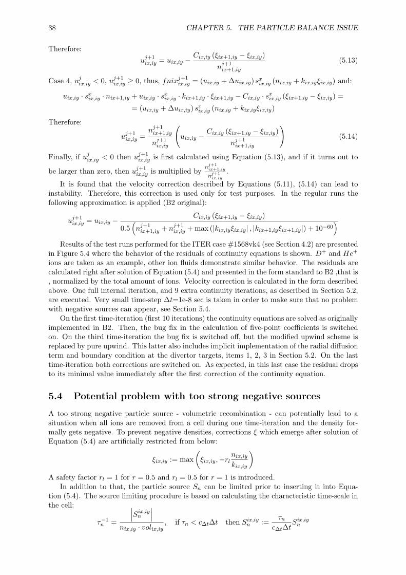
Results of the test runs performed for the ITER case #1568vk4 (see Section 4.2) are presentedin Figure 5.4 where the behavior of the residuals of continuity equations is shown. D+ and He+

ions are taken as an example, other ion fluids demonstrate similar behavior. The residuals arecalculated right after solution of Equation (5.4) and presented in the form standard to B2 ,that is, normalized by the total amount of ions. Velocity correction is calculated in the form describedabove. One full internal iteration, and 9 extra continuity iterations, as described in Section 5.2,are executed. Very small time-step ∆t=1e-8 sec is taken in order to make sure that no problemwith negative sources can appear, see Section 5.4.

On the first time-iteration (first 10 iterations) the continuity equations are solved as originallyimplemented in B2. Then, the bug fix in the calculation of five-point coefficients is switchedon. On the third time-iteration the bug fix is switched off, but the modified upwind scheme isreplaced by pure upwind. This latter also includes implicit implementation of the radial diffusionterm and boundary condition at the divertor targets, items 1, 2, 3 in Section 5.2. On the lasttime-iteration both corrections are switched on. As expected, in this last case the residual dropsto its minimal value immediately after the first correction of the continuity equation.

5.4 Potential problem with too strong negative sources

A too strong negative particle source - volumetric recombination - can potentially lead to asituation when all ions are removed from a cell during one time-iteration and the density for-mally gets negative. To prevent negative densities, corrections ξ which emerge after solution ofEquation (5.4) are artificially restricted from below:

ξix,iy := max

(ξix,iy,−rl

nix,iykix,iy

)A safety factor rl = 1 for r = 0.5 and rl = 0.5 for r = 1 is introduced.

In addition to that, the particle source Sn can be limited prior to inserting it into Equa-tion (5.4). The source limiting procedure is based on calculating the characteristic time-scale inthe cell:

τ−1n =

∣∣∣Six,iyn

∣∣∣nix,iy · volix,iy

, if τn < c∆t∆t then Six,iyn :=

τnc∆t∆t

Six,iyn

5.4. POTENTIAL PROBLEM WITH TOO STRONG NEGATIVE SOURCES 39

(a) D+ (b) He+

Figure 5.4: Residuals of the continuity equation for (a) D+ and (b) He+. Test of the particlebalance correction schemes. The numbers stand for the grid regions: 01 is the core, 02 is thescrape-off-layer, 03 is the inner divertor leg and 04 is the outer divertor leg

The whole source profile is the re-scaled to keep the same total source strength (integral over thegrid) the same as before correction. A limiting factor c∆t = 0.01 is typically used. It has beenfound that this procedure can significantly distort the final solution in the cases with strongvolumetric recombination when a large time-step ∆t is applied. In the test runs discussed in thepresent report c∆t was always set to 0: that is, no artificial source limitation is applied at all.

The source limitation has been replaced by an automatic reduction of the time-step in thecells where the sources are too strong. The same time-step ∆tβix,iy is always applied for all ionfluids which belong to the species β. The correction follows from the cell particle balance:

nβix,iy − nβix,iy

∆tβix,iy+ Γβ

ix,iy = Sβix,iy

Here:

Γβix,iy =

∑α′

(fnixα

′ix,iy − fnixα

′ix−1,iy + fniyα

′ix,iy − fniyα

′ix,iy−1

)nβix,iy =

∑α′

nα′

ix,iy, Sβix,iy =

∑α′

Sα′n (ix, iy)

The sums are calculated over all ion fluids of species β, nβix,iy is the expected value at theend of the time-iteration, boundary (guard) cells are excluded from this correction. Condition

nβix,iy > 0 yields:

nβix,iy = nβix,iy +(Sβix,iy − Γβ

ix,iy

)∆tβix,iy > 0

This inequality is fulfilled automatically if Sβix,iy > Γβ

ix,iy (since nβix,iy > 0). Otherwise:

nβix,iy +(Sβix,iy − Γβ

ix,iy

)∆tβix,iy > 0 ⇒ ∆tβix,iy <

nβix,iy

Γβix,iy − Sβ

ix,iy

= ∆tmax (5.15)

If Sβix,iy < Γβ

ix,iy then the local time-step is modified as follows:

if ∆t > ∆tmax then ∆tix,iy = 0.5∆tmax (5.16)


The correction is applied on internal iterations each time after solving Equation (5.4) for eachspecies.

Experience has shown that even in the run with strong volumetric recombination discussedin Section 6.4 below Equations (5.15), (5.16) never led to correction of local time-step for D+

ions. Therefore, in the test runs in question this option was normally switched off.

5.5 Can a simplified (0D) correction be applied?

Instead of solving the spatially resolved continuity equations, as described in Section 5.2, onecould multiply the whole density profile with a single scaling factor and obtain formally zeroerror in the global particle balance on the CFD side. The scaling factor ζn for each plasmaspecies can be found from the solution of the following equation (written for time-iteration kand internal iteration j):

Γconst + Γoutζn = Sntot +N0

∆t −N∆tζn (5.17)

Where:

Γout =∑α′

∑i

(Sα′n (j, k) +

nα′ (j, k)

∆t− nα′ (0, k)

∆t−Rα′

n (j, k)

)− Γconst

Sntot =

∑α′

∑i

Sα′n (j, k) , N0

∆t =∑α′

∑i

nα′ (0, k)

∆t, N∆t =

∑α′

∑i

nα′ (j, k)

∆t

The sum is calculated over all cells i and ion fluids α′, the time-step ∆t can be spatially non-uniform. The correction is based on the assumption that the outflux from the computationalgrid is directly proportional to the density. On boundaries where e.g. constant flux boundaryconditions are specified this condition is not fulfilled. Outflux at such boundaries is taken intoaccount separately in Γconst.

The correction has been implemented in B2 at the end of internal iterations. Scaling factorζn is calculated from Equation (5.17), then the density nα‘ in each cell is multiplied by ζn -a special treatment is required at the boundaries for some types of boundary conditions, thesources Sα′

n are re-calculated, Equation (1.8), and the iteration is repeated. Approximately 10such iterations are typically required.

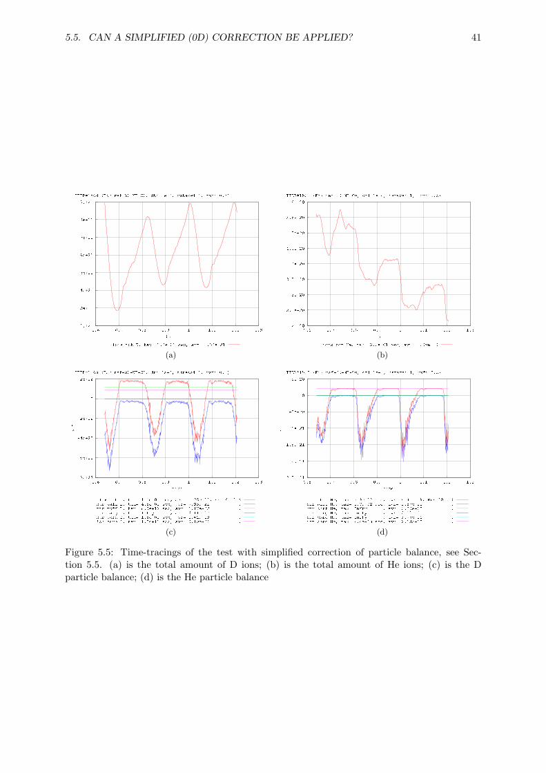
The correction has been tested for the case #1568vk4, same as in Section 4.2. The test hasindicated that this procedure leads to long-period self-sustained oscillations and no steady-statesolution can be obtained. An example is shown in Figure 5.5 which represents time-traces fromthe run made with time-step ∆t =1e-4 sec and 1e-3 sec in the core. A run with ∆t =1e-4 sec inthe whole computational has been made as well, but was not continued after one period of similaroscillations was detected. It can be concluded that the correction based on Equation (5.17) isnot applicable in practice.

5.5. CAN A SIMPLIFIED (0D) CORRECTION BE APPLIED? 41

(a) (b)

(c) (d)

Figure 5.5: Time-tracings of the test with simplified correction of particle balance, see Sec-tion 5.5. (a) is the total amount of D ions; (b) is the total amount of He ions; (c) is the Dparticle balance; (d) is the He particle balance


Chapter 6

Case studies

6.1 Tests with extra continuity iterations

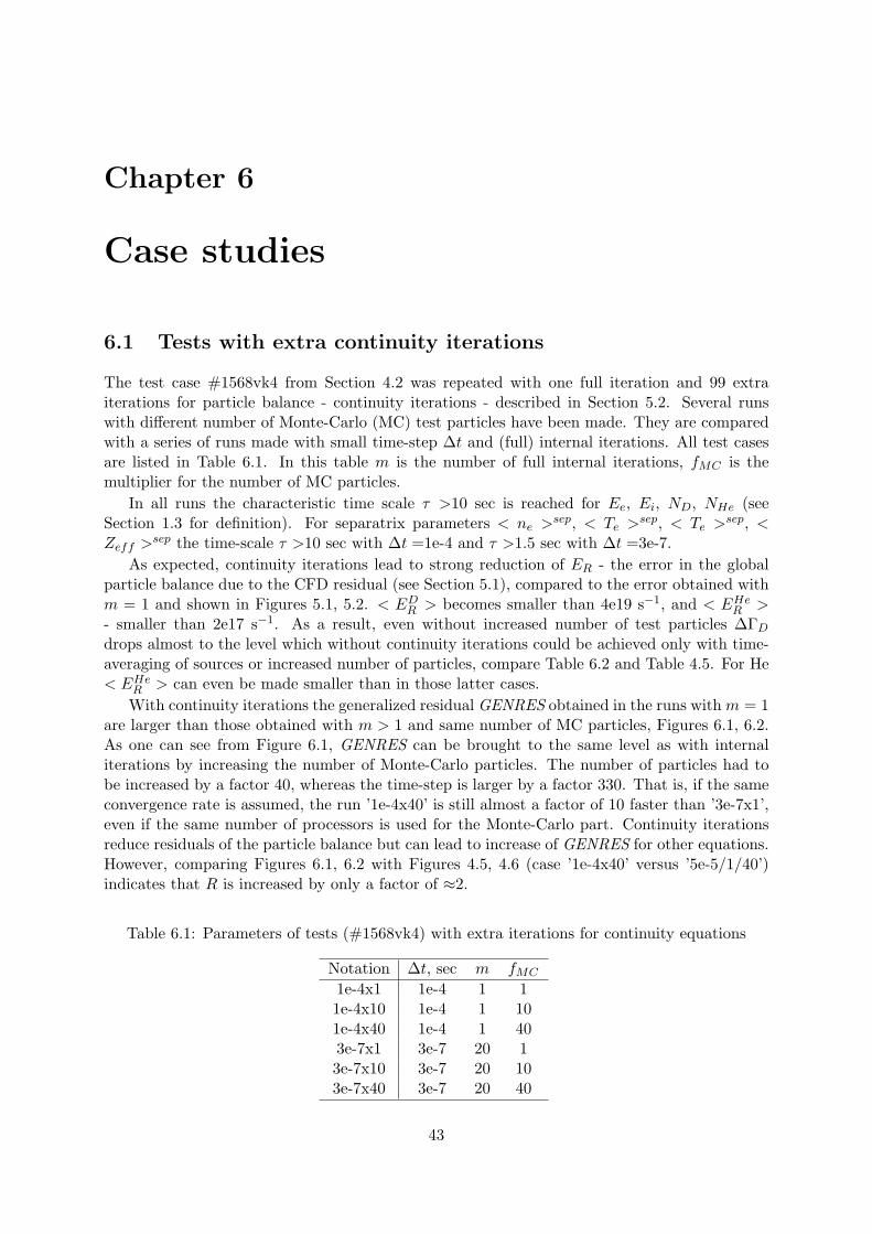
The test case #1568vk4 from Section 4.2 was repeated with one full iteration and 99 extraiterations for particle balance - continuity iterations - described in Section 5.2. Several runswith different number of Monte-Carlo (MC) test particles have been made. They are comparedwith a series of runs made with small time-step ∆t and (full) internal iterations. All test casesare listed in Table 6.1. In this table m is the number of full internal iterations, fMC is themultiplier for the number of MC particles.

In all runs the characteristic time scale τ >10 sec is reached for Ee, Ei, ND, NHe (seeSection 1.3 for definition). For separatrix parameters < ne >

sep, < Te >sep, < Te >

sep, <Zeff >

sep the time-scale τ >10 sec with ∆t =1e-4 and τ >1.5 sec with ∆t =3e-7.

As expected, continuity iterations lead to strong reduction of ER - the error in the globalparticle balance due to the CFD residual (see Section 5.1), compared to the error obtained withm = 1 and shown in Figures 5.1, 5.2. < ED

R > becomes smaller than 4e19 s−1, and < EHeR >

- smaller than 2e17 s−1. As a result, even without increased number of test particles ∆ΓD

drops almost to the level which without continuity iterations could be achieved only with time-averaging of sources or increased number of particles, compare Table 6.2 and Table 4.5. For He< EHe

R > can even be made smaller than in those latter cases.

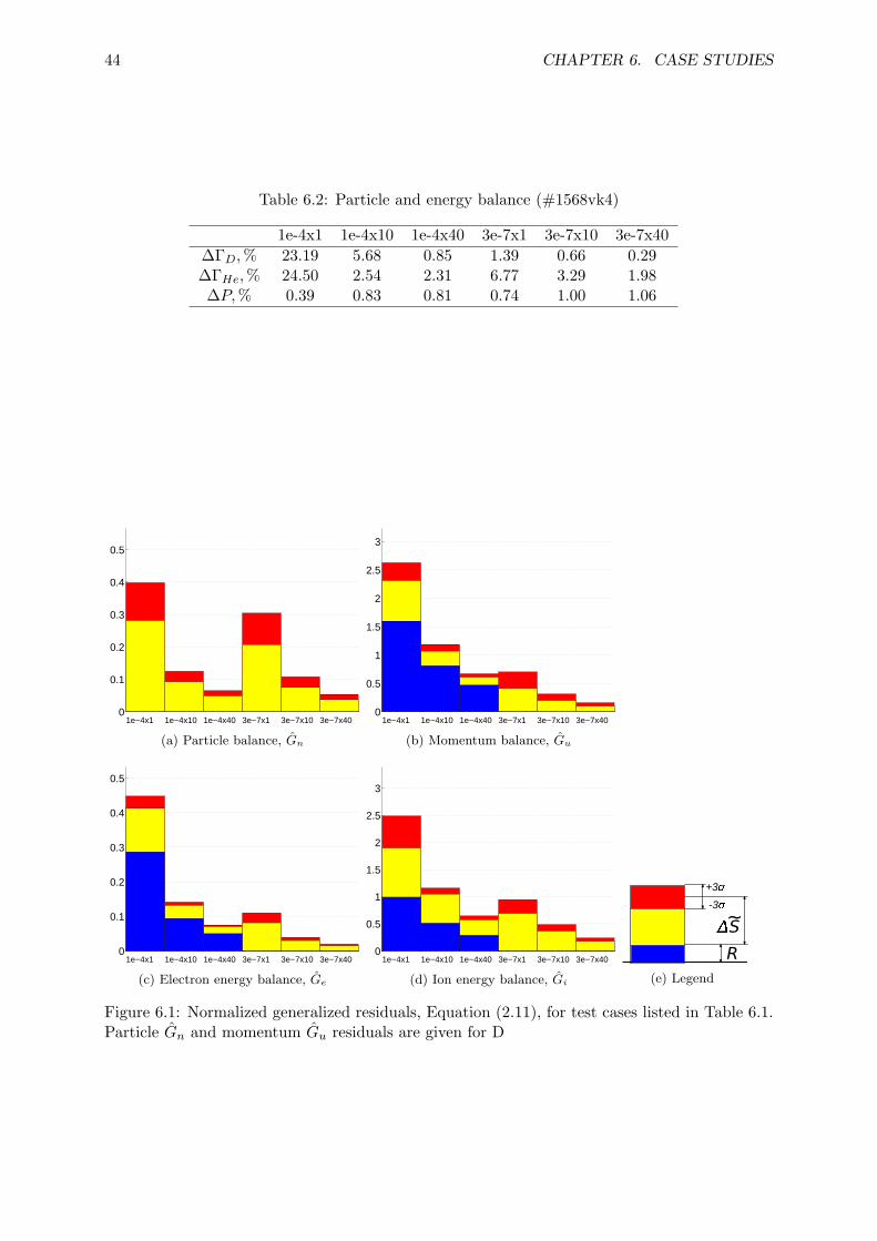
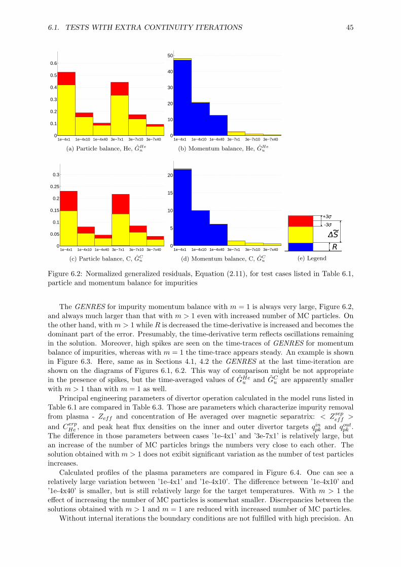
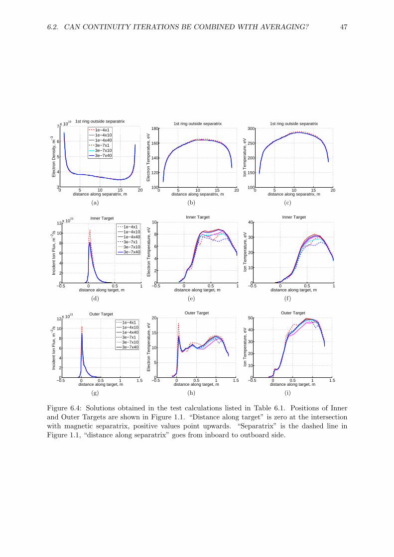
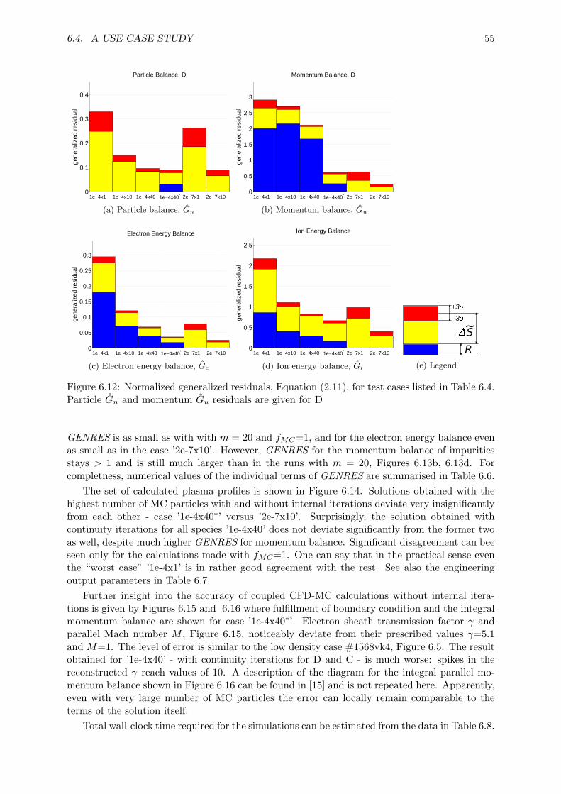
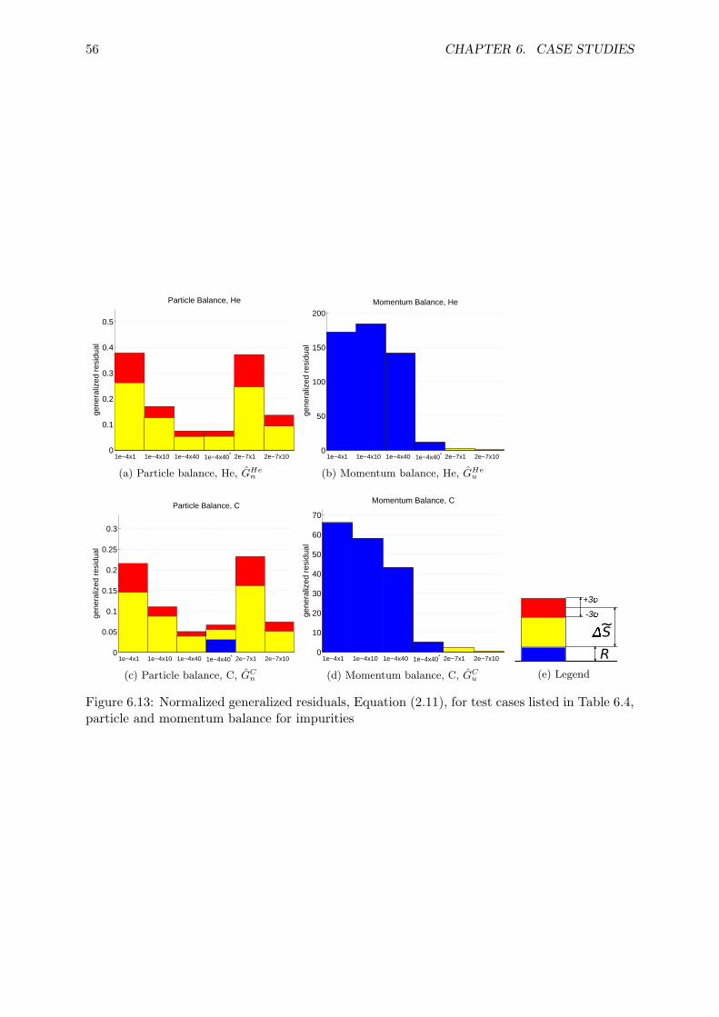
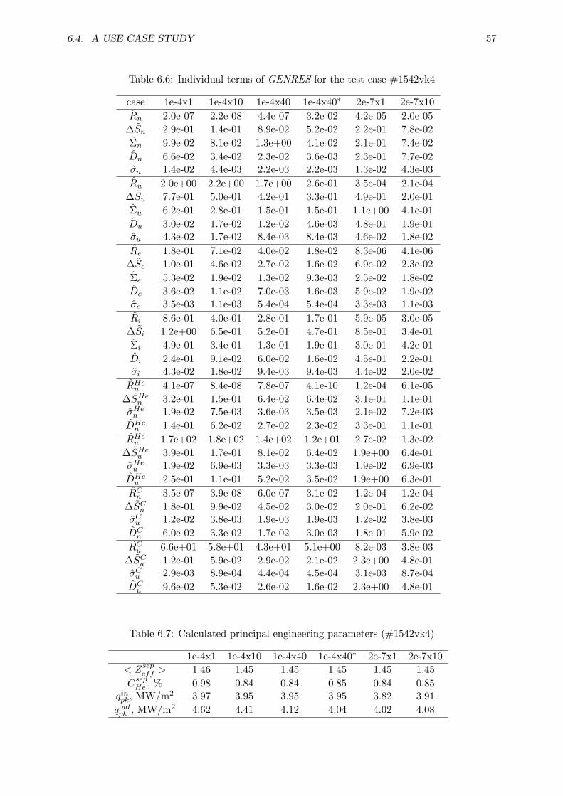
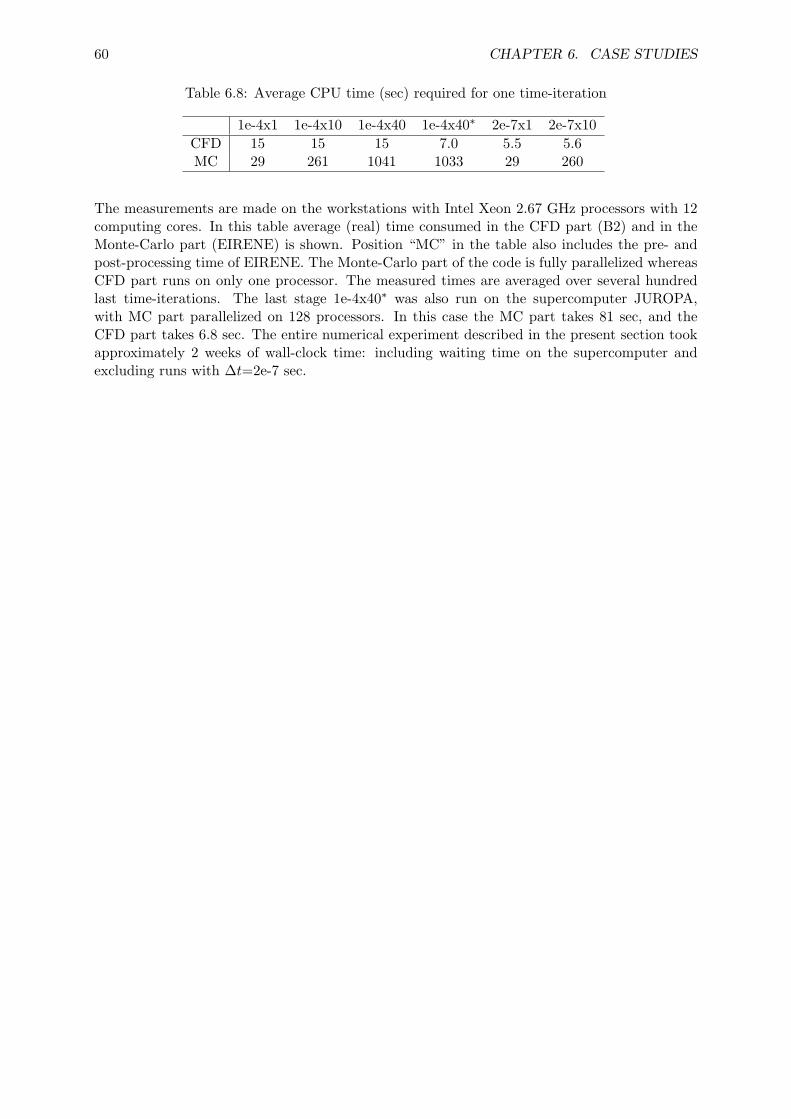
With continuity iterations the generalized residual GENRES obtained in the runs withm = 1are larger than those obtained with m > 1 and same number of MC particles, Figures 6.1, 6.2.As one can see from Figure 6.1, GENRES can be brought to the same level as with internaliterations by increasing the number of Monte-Carlo particles. The number of particles had tobe increased by a factor 40, whereas the time-step is larger by a factor 330. That is, if the sameconvergence rate is assumed, the run ’1e-4x40’ is still almost a factor of 10 faster than ’3e-7x1’,even if the same number of processors is used for the Monte-Carlo part. Continuity iterationsreduce residuals of the particle balance but can lead to increase of GENRES for other equations.However, comparing Figures 6.1, 6.2 with Figures 4.5, 4.6 (case ’1e-4x40’ versus ’5e-5/1/40’)indicates that R is increased by only a factor of ≈2.

Table 6.1: Parameters of tests (#1568vk4) with extra iterations for continuity equations

Notation ∆t, sec m fMC

1e-4x1 1e-4 1 11e-4x10 1e-4 1 101e-4x40 1e-4 1 403e-7x1 3e-7 20 13e-7x10 3e-7 20 103e-7x40 3e-7 20 40

43

44 CHAPTER 6. CASE STUDIES


1e-4x1 1e-4x10 1e-4x40 3e-7x1 3e-7x10 3e-7x40

∆ΓD,% 23.19 5.68 0.85 1.39 0.66 0.29∆ΓHe,% 24.50 2.54 2.31 6.77 3.29 1.98∆P,% 0.39 0.83 0.81 0.74 1.00 1.06

0

0.1

0.2

0.3

0.4

0.5

1e−4x1 1e−4x10 1e−4x40 3e−7x1 3e−7x10 3e−7x40


0

0.5

1

1.5

2

2.5

3

1e−4x1 1e−4x10 1e−4x40 3e−7x1 3e−7x10 3e−7x40


0

0.1

0.2

0.3

0.4

0.5

1e−4x1 1e−4x10 1e−4x40 3e−7x1 3e−7x10 3e−7x40


0

0.5

1

1.5

2

2.5

3

1e−4x1 1e−4x10 1e−4x40 3e−7x1 3e−7x10 3e−7x40


R

S

+3�

-3�

~

(e) Legend


6.1. TESTS WITH EXTRA CONTINUITY ITERATIONS 45

0

0.1

0.2

0.3

0.4

0.5

0.6

1e−4x1 1e−4x10 1e−4x40 3e−7x1 3e−7x10 3e−7x40


0

10

20

30

40

50

1e−4x1 1e−4x10 1e−4x40 3e−7x1 3e−7x10 3e−7x40


0

0.05

0.1

0.15

0.2

0.25

0.3

1e−4x1 1e−4x10 1e−4x40 3e−7x1 3e−7x10 3e−7x40


0

5

10

15

20

1e−4x1 1e−4x10 1e−4x40 3e−7x1 3e−7x10 3e−7x40


R

S

+3�

-3�

~

(e) Legend


The GENRES for impurity momentum balance with m = 1 is always very large, Figure 6.2,and always much larger than that with m > 1 even with increased number of MC particles. Onthe other hand, withm > 1 while R is decreased the time-derivative is increased and becomes thedominant part of the error. Presumably, the time-derivative term reflects oscillations remainingin the solution. Moreover, high spikes are seen on the time-traces of GENRES for momentumbalance of impurities, whereas with m = 1 the time-trace appears steady. An example is shownin Figure 6.3. Here, same as in Sections 4.1, 4.2 the GENRES at the last time-iteration areshown on the diagrams of Figures 6.1, 6.2. This way of comparison might be not appropriatein the presence of spikes, but the time-averaged values of GHe

u and GCu are apparently smaller

with m > 1 than with m = 1 as well.

Principal engineering parameters of divertor operation calculated in the model runs listed inTable 6.1 are compared in Table 6.3. Those are parameters which characterize impurity removalfrom plasma - Zeff and concentration of He averaged over magnetic separatrix: < Zsep

eff >

and CerpHe , and peak heat flux densities on the inner and outer divertor targets qinpk and qoutpk .

The difference in those parameters between cases ’1e-4x1’ and ’3e-7x1’ is relatively large, butan increase of the number of MC particles brings the numbers very close to each other. Thesolution obtained with m > 1 does not exibit significant variation as the number of test particlesincreases.

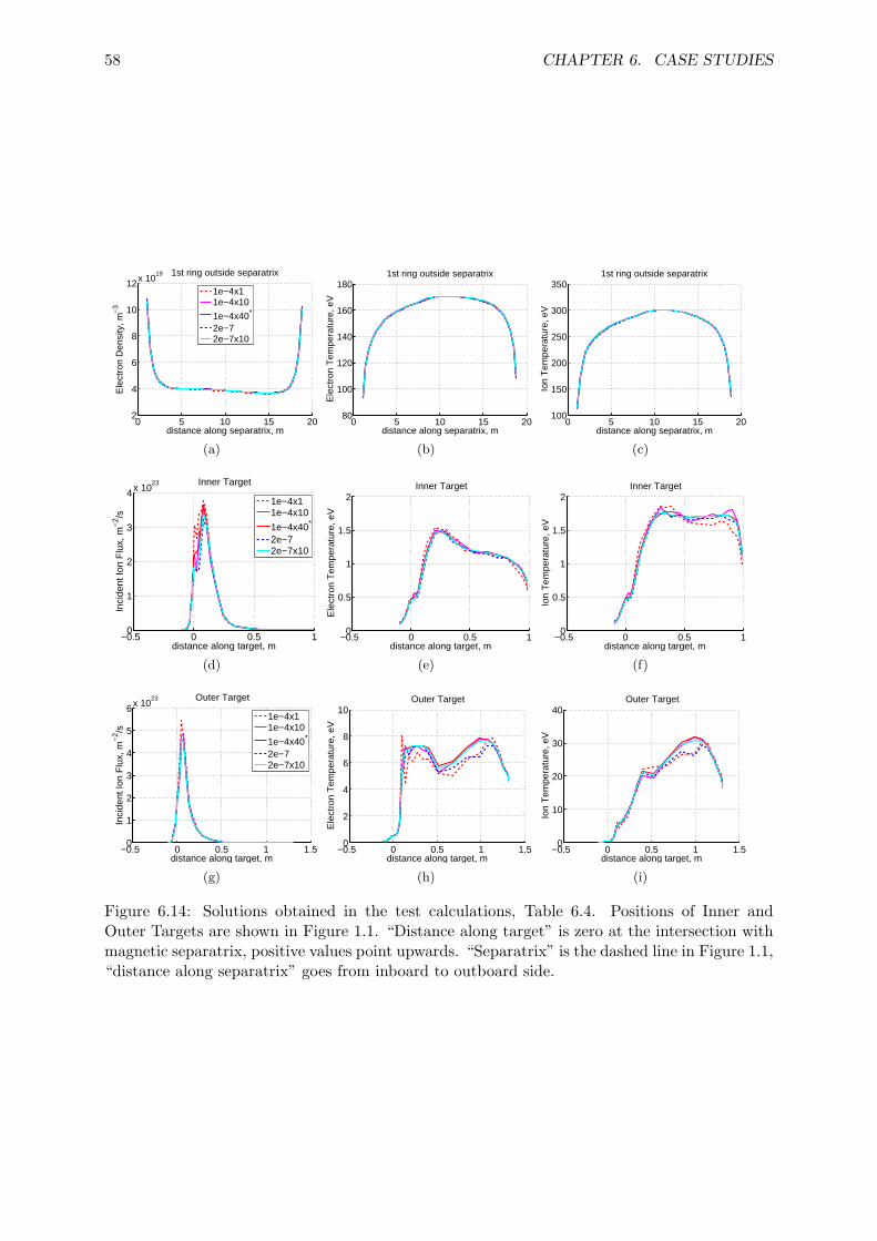
Calculated profiles of the plasma parameters are compared in Figure 6.4. One can see arelatively large variation between ’1e-4x1’ and ’1e-4x10’. The difference between ’1e-4x10’ and’1e-4x40’ is smaller, but is still relatively large for the target temperatures. With m > 1 theeffect of increasing the number of MC particles is somewhat smaller. Discrepancies between thesolutions obtained with m > 1 and m = 1 are reduced with increased number of MC particles.

Without internal iterations the boundary conditions are not fulfilled with high precision. An


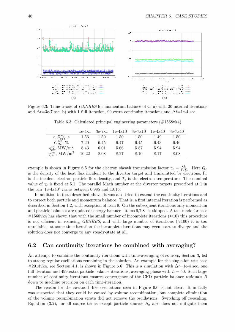
(a) (b)

Figure 6.3: Time-traces of GENRES for momentum balance of C: a) with 20 internal iterationsand ∆t=3e-7 sec; b) with 1 full iteration, 99 extra continuity iterations and ∆t=1e-4 sec.

Table 6.3: Calculated principal engineering parameters (#1568vk4)

1e-4x1 3e-7x1 1e-4x10 3e-7x10 1e-4x40 3e-7x40

< Zsepeff > 1.53 1.50 1.50 1.50 1.49 1.50

CsepHe , % 7.20 6.45 6.47 6.45 6.43 6.46

qinpk, MW/m2 8.43 6.01 5.66 5.87 5.94 5.94

qoutpk , MW/m2 10.22 8.08 8.27 8.10 8.17 8.08

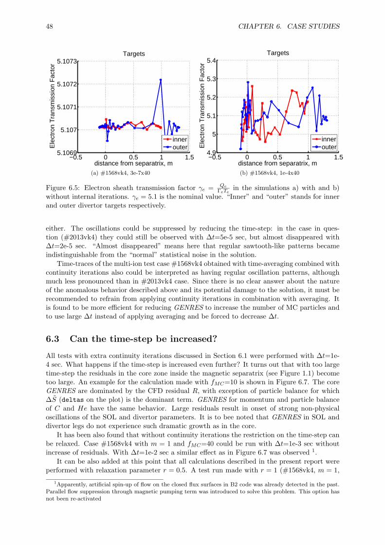
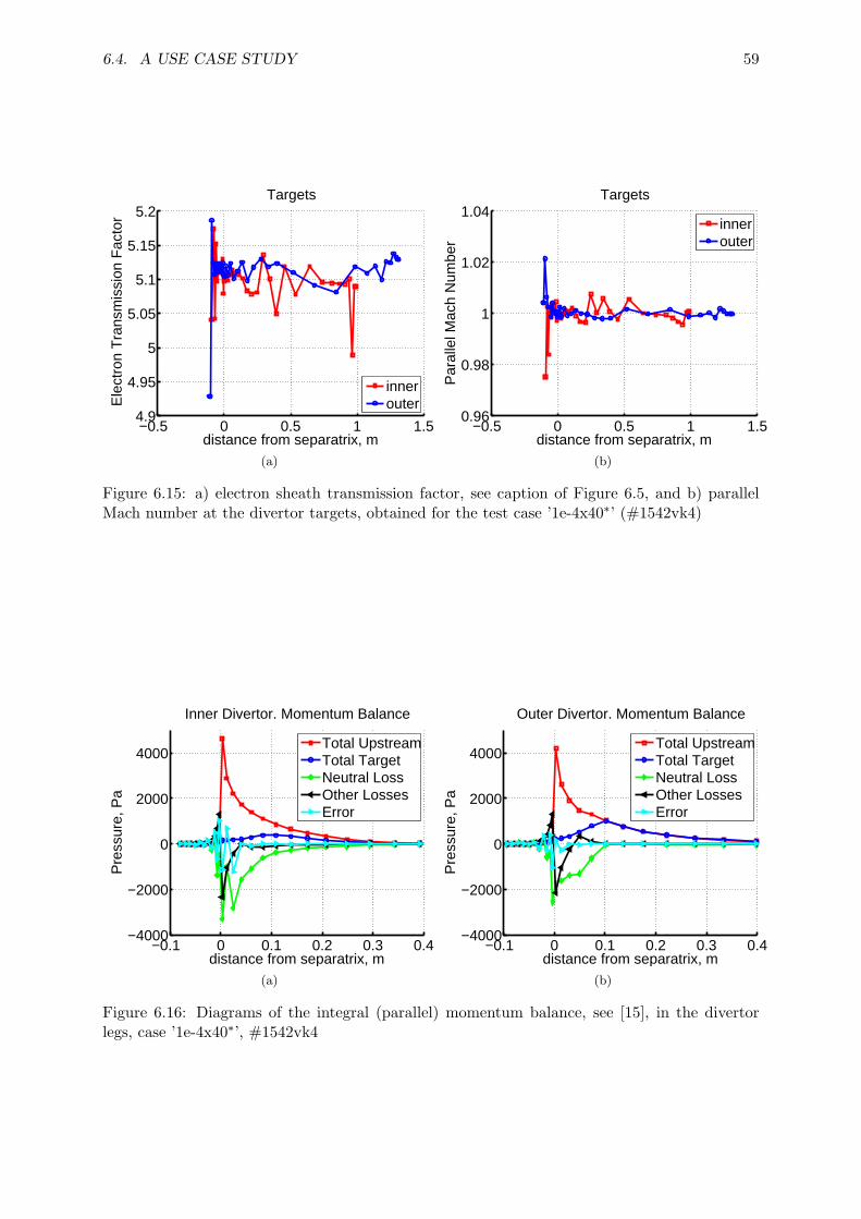
example is shown in Figure 6.5 for the electron sheath transmission factor γe = Qe

ΓeTe. Here Qe

is the density of the heat flux incident to the divertor target and transmitted by electrons, Γe

is the incident electron particle flux density, and Te is the electron temperature. The nominalvalue of γe is fixed at 5.1. The parallel Mach number at the divertor targets prescribed at 1 inthe run ’1e-4x40’ varies between 0.985 and 1.015.

In addition to tests described above, it was also tried to extend the continuity iterations andto correct both particle and momentum balance. That is, a first internal iteration is performed asdescribed in Section 1.2, with exception of item 9. On the subsequent iterations only momentumand particle balances are updated: energy balance - items 6,7,8 - is skipped. A test made for case#1568vk4 has shown that with the small number of incomplete iterations (≈10) this procedureis not efficient in reducing GENRES, and with large number of iterations (≈100) it is toounreliable: at some time-iteration the incomplete iterations may even start to diverge and thesolution does not converge to any steady-state at all.

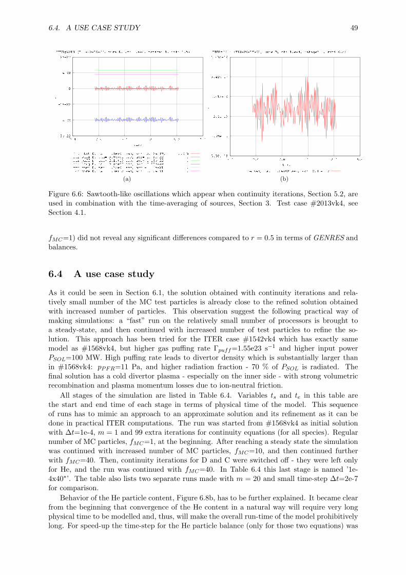
6.2 Can continuity iterations be combined with averaging?

An attempt to combine the continuity iterations with time-averaging of sources, Section 3, ledto strong regular oscillations remaining in the solution. An example for the single-ion test case#2013vk4, see Section 4.1, is shown in Figure 6.6. This is a simulation with ∆t=1e-4 sec, onefull iteration and 499 extra particle balance iterations, averaging phase with L = 50. Such largenumber of continuity iterations ensures convergence of the CFD particle balance residuals Rdown to machine precision on each time-iteration.

The reason for the sawtooth-like oscillations seen in Figure 6.6 is not clear. It initiallywas suspected that they could be caused by volume recombination, but complete eliminationof the volume recombination strata did not remove the oscillations. Switching off re-scaling,Equation (3.2), for all source terms except particle sources Sn also does not mitigate them

6.2. CAN CONTINUITY ITERATIONS BE COMBINED WITH AVERAGING? 47

0 5 10 15 203

4

5

6



Ele

ctro

n D

ensi

ty, m

−3

1e−4x11e−4x101e−4x403e−7x13e−7x103e−7x40

(a)

0 5 10 15 20100

120

140

160



Ele

ctro

n T

empe

ratu

re, e

V

(b)

0 5 10 15 20100

150

200

250



Ion

Tem

pera

ture

, eV

(c)

−0.5 0 0.5 10

2

4

6

8

10



Inci

dent

Ion

Flu

x, m

−2 /s

1e−4x11e−4x101e−4x403e−7x13e−7x103e−7x40

(d)

−0.5 0 0.5 10

2

4

6

8

10Inner Target


Ele

ctro

n T

empe

ratu

re, e

V

(e)

−0.5 0 0.5 10

10

20

30

40Inner Target


Ion

Tem

pera

ture

, eV

(f)

−0.5 0 0.5 1 1.50

2

4

6

8

10



Inci

dent

Ion

Flu

x, m

−2 /s

1e−4x11e−4x101e−4x403e−7x13e−7x103e−7x40

(g)

−0.5 0 0.5 1 1.50

5

10

15

20Outer Target


Ele

ctro

n T

empe

ratu

re, e

V

(h)

−0.5 0 0.5 1 1.50

10

20

30

40

50Outer Target


Ion

Tem

pera

ture

, eV

(i)

Figure 6.4: Solutions obtained in the test calculations listed in Table 6.1. Positions of Innerand Outer Targets are shown in Figure 1.1. “Distance along target” is zero at the intersectionwith magnetic separatrix, positive values point upwards. “Separatrix” is the dashed line inFigure 1.1, “distance along separatrix” goes from inboard to outboard side.


−0.5 0 0.5 1 1.55.1069

5.107

5.1071

5.1072

5.1073Targets

distance from separatrix, m

Ele

ctro

n T

rans

mis

sion

Fac

tor

innerouter

(a) #1568vk4, 3e-7x40

−0.5 0 0.5 1 1.54.9

5

5.1

5.2

5.3

5.4Targets


Ele

ctro

n T

rans

mis

sion

Fac

tor

innerouter

(b) #1568vk4, 1e-4x40

Figure 6.5: Electron sheath transmission factor γe = Qe

ΓeTein the simulations a) with and b)

without internal iterations. γe = 5.1 is the nominal value. “Inner” and “outer” stands for innerand outer divertor targets respectively.

either. The oscillations could be suppressed by reducing the time-step: in the case in ques-tion (#2013vk4) they could still be observed with ∆t=5e-5 sec, but almost disappeared with∆t=2e-5 sec. “Almost disappeared” means here that regular sawtooth-like patterns becameindistinguishable from the “normal” statistical noise in the solution.

Time-traces of the multi-ion test case #1568vk4 obtained with time-averaging combined withcontinuity iterations also could be interpreted as having regular oscillation patterns, althoughmuch less pronounced than in #2013vk4 case. Since there is no clear answer about the natureof the anomalous behavior described above and its potential damage to the solution, it must berecommended to refrain from applying continuity iterations in combination with averaging. Itis found to be more efficient for reducing GENRES to increase the number of MC particles andto use large ∆t instead of applying averaging and be forced to decrease ∆t.

6.3 Can the time-step be increased?

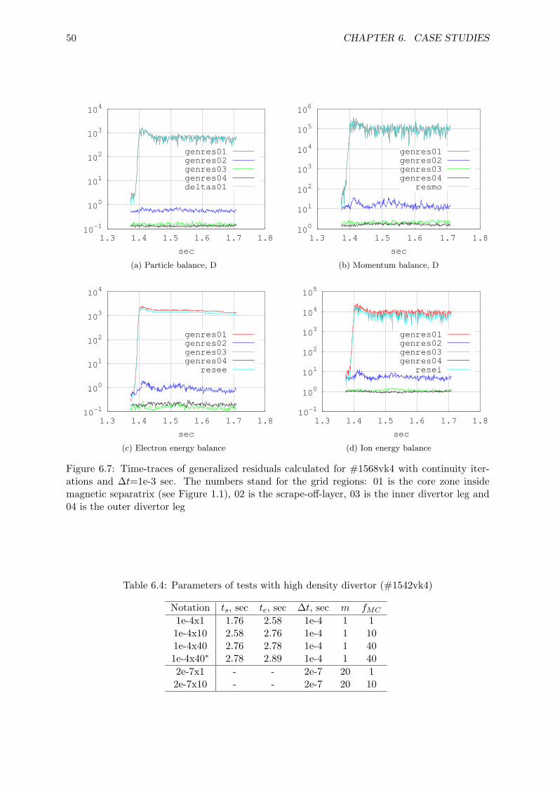
All tests with extra continuity iterations discussed in Section 6.1 were performed with ∆t=1e-4 sec. What happens if the time-step is increased even further? It turns out that with too largetime-step the residuals in the core zone inside the magnetic separatrix (see Figure 1.1) becometoo large. An example for the calculation made with fMC=10 is shown in Figure 6.7. The coreGENRES are dominated by the CFD residual R, with exception of particle balance for which∆S (deltas on the plot) is the dominant term. GENRES for momentum and particle balanceof C and He have the same behavior. Large residuals result in onset of strong non-physicaloscillations of the SOL and divertor parameters. It is to bee noted that GENRES in SOL anddivertor legs do not experience such dramatic growth as in the core.

It has been also found that without continuity iterations the restriction on the time-step canbe relaxed. Case #1568vk4 with m = 1 and fMC=40 could be run with ∆t=1e-3 sec withoutincrease of residuals. With ∆t=1e-2 sec a similar effect as in Figure 6.7 was observed 1.

It can be also added at this point that all calculations described in the present report wereperformed with relaxation parameter r = 0.5. A test run made with r = 1 (#1568vk4, m = 1,

1Apparently, artificial spin-up of flow on the closed flux surfaces in B2 code was already detected in the past.Parallel flow suppression through magnetic pumping term was introduced to solve this problem. This option hasnot been re-activated

6.4. A USE CASE STUDY 49

(a) (b)

Figure 6.6: Sawtooth-like oscillations which appear when continuity iterations, Section 5.2, areused in combination with the time-averaging of sources, Section 3. Test case #2013vk4, seeSection 4.1.

fMC=1) did not reveal any significant differences compared to r = 0.5 in terms of GENRES andbalances.

6.4 A use case study

As it could be seen in Section 6.1, the solution obtained with continuity iterations and rela-tively small number of the MC test particles is already close to the refined solution obtainedwith increased number of particles. This observation suggest the following practical way ofmaking simulations: a “fast” run on the relatively small number of processors is brought toa steady-state, and then continued with increased number of test particles to refine the so-lution. This approach has been tried for the ITER case #1542vk4 which has exactly samemodel as #1568vk4, but higher gas puffing rate Γpuff=1.55e23 s−1 and higher input powerPSOL=100 MW. High puffing rate leads to divertor density which is substantially larger thanin #1568vk4: pPFR=11 Pa, and higher radiation fraction - 70 % of PSOL is radiated. Thefinal solution has a cold divertor plasma - especially on the inner side - with strong volumetricrecombination and plasma momentum losses due to ion-neutral friction.

All stages of the simulation are listed in Table 6.4. Variables ts and te in this table arethe start and end time of each stage in terms of physical time of the model. This sequenceof runs has to mimic an approach to an approximate solution and its refinement as it can bedone in practical ITER computations. The run was started from #1568vk4 as initial solutionwith ∆t=1e-4, m = 1 and 99 extra iterations for continuity equations (for all species). Regularnumber of MC particles, fMC=1, at the beginning. After reaching a steady state the simulationwas continued with increased number of MC particles, fMC=10, and then continued furtherwith fMC=40. Then, continuity iterations for D and C were switched off - they were left onlyfor He, and the run was continued with fMC=40. In Table 6.4 this last stage is named ’1e-4x40∗’. The table also lists two separate runs made with m = 20 and small time-step ∆t=2e-7for comparison.

Behavior of the He particle content, Figure 6.8b, has to be further explained. It became clearfrom the beginning that convergence of the He content in a natural way will require very longphysical time to be modelled and, thus, will make the overall run-time of the model prohibitivelylong. For speed-up the time-step for the He particle balance (only for those two equations) was


10-1

100

101

102

103

104

1.3 1.4 1.5 1.6 1.7 1.8

sec

genres01genres02genres03genres04deltas01

(a) Particle balance, D

100

101

102

103

104

105

106

1.3 1.4 1.5 1.6 1.7 1.8

sec

genres01genres02genres03genres04

resmo

(b) Momentum balance, D

10-1

100

101

102

103

104

1.3 1.4 1.5 1.6 1.7 1.8

sec


resee


10-1

100

101

102

103

104

105

1.3 1.4 1.5 1.6 1.7 1.8

sec


resei

(d) Ion energy balance

Figure 6.7: Time-traces of generalized residuals calculated for #1568vk4 with continuity iter-ations and ∆t=1e-3 sec. The numbers stand for the grid regions: 01 is the core zone insidemagnetic separatrix (see Figure 1.1), 02 is the scrape-off-layer, 03 is the inner divertor leg and04 is the outer divertor leg

Table 6.4: Parameters of tests with high density divertor (#1542vk4)

Notation ts, sec te, sec ∆t, sec m fMC

1e-4x1 1.76 2.58 1e-4 1 11e-4x10 2.58 2.76 1e-4 1 101e-4x40 2.76 2.78 1e-4 1 401e-4x40∗ 2.78 2.89 1e-4 1 40

2e-7x1 - - 2e-7 20 12e-7x10 - - 2e-7 20 10


1.6 1.8 2 2.2 2.4 2.6 2.8 37

7.2

7.4

7.6

7.8

8

8.2

8.4

8.6

8.8

9x 10

21 Total number of ions, D

sec

(a)

1.6 1.8 2 2.2 2.4 2.6 2.8 30.5

1

1.5

2

2.5

3

3.5

4

4.5

5

5.5x 10

20 Total number of ions, He

sec

(b)

1.6 1.8 2 2.2 2.4 2.6 2.8 31.05

1.1

1.15

1.2

1.25

1.3

1.35

1.4

1.45

1.5x 10

20 Total number of ions, C

sec

(c)

1.6 1.8 2 2.2 2.4 2.6 2.8 31.3

1.35

1.4

1.45

1.5

1.55

1.6

1.65

1.7

1.75x 10

6

sec

Tot

al e

nerg

y, J

electronsions

(d)

Figure 6.8: Time-tracings of the total number of ions and total diamagnetic energy. Case#1542vk4 , Table 6.4

increased to 1e-3 sec. This increase of ∆tHe manifests itself as rapid drop of the number of Heions between t =1.87 sec t =1.99 sec. Further, traces of some negative effects on the momentumbalance have been noticed, therefore, as a precaution measure at t =1.99 sec ∆tHe was returnedback to 1e-4 sec and the He particle balance was converged further in the natural way. Itcannot be said with certainty that the applied way of speeding up the He convergence wasindeed harmful - the issue was not further investigated. At t =2.67 sec another speed-up trickwas used: multiplication of the initial He density by a factor 0.9 when the run is re-started forcontinuation. The effect of this multiplication is seen as step in Figure 6.8b.

Time-tracings of the run which include all stages are presented in Figures 6.8-6.10. Char-acteristic times (see Section 1.3) at the end of each stage are >9 sec (>4 sec for NHe, NC).As expected, the residuals (GENRES) are reduced with increased number of particles, Fig-ures 6.10, 6.11. However, for momentum balance this reduction is apparently less than by afactor

√fMC . From Figures 6.12, 6.13 where diagrams of GENRES at the end of each stage

are shown it becomes apparent that R for momentum balance practically does not reduce withincreased fMC , and the values are large, especially for impurities.


1.6 1.8 2 2.2 2.4 2.6 2.8 3−3

−2.5

−2

−1.5

−1

−0.5

0

0.5

1

1.5

2x 10

23 Particle balance, D

sec

s−1

∆ ΓΓ

pump

Γnout

(a)

1.6 1.8 2 2.2 2.4 2.6 2.8 3−3

−2.5

−2

−1.5

−1

−0.5

0

0.5x 10

21 Particle balance, He

sec

s−1

∆ ΓΓ

pump

Γnout

(b)

1.6 1.8 2 2.2 2.4 2.6 2.8 3−2.5

−2

−1.5

−1

−0.5

0

0.5

1

1.5

2

2.5x 10

22 Particle balance, C

sec

s−1

∆ ΓΓ

pump

Γnout

(c)

1.6 1.8 2 2.2 2.4 2.6 2.8 3−2

0

2

4

6

8

10x 10

7

sec

W

∆ PP

rad

PPFC

(d)

Figure 6.9: Time-tracings of the particle and energy balance, see Equations (1.9) and (1.10),Section 1.3. Case #1542vk4, Table 6.4


1e-4x1 1e-4x10 1e-4x40 1e-4x40∗ 2e-7x1 2e-7x10

∆ΓD,% 1.40 0.70 1.82 0.20 0.59 1.46∆ΓHe,% 4.72 3.45 3.26 3.14 7.07 4.96∆P,% 0.39 0.43 0.33 0.49 0.33 0.34


1.5 2 2.5 310

−4

10−3

10−2

10−1

100

electron energy balance

sec

GR∆ SσDT

(a)

1.5 2 2.5 310

−3

10−2

10−1

100

101

ion energy balance

sec

(b)

1.5 2 2.5 310

−10

10−5

100

particle balance, D

sec

(c)

1.5 2 2.5 310

−3

10−2

10−1

100

101

momentum balance, D

sec

(d)

Figure 6.10: Time-tracings of GENRES for energy and main ions, case #1542vk4 , Table 6.4.In the legend G, R, ∆S and σ are normalized generalized residuals G and its terms R, ∆S andσ, Equation (2.9), DT is the time derivative (included in ∆S)

The decision to continue the simulation with continuity iterations kept only for He wasbased on two considerations. First, it was suspected that continuity iterations could be themain reason of “damaging” the momentum balance. Second, one could see that with fMC=40already for the low-density case, Section 4.2, the error in the particle balance for main ionsis almost on acceptable level, and the relative error is expected to be smaller with higher gaspuffing rate. To stay on the safe side, continuity iterations were left for He. The test results haveconfirmed those considerations. Without continuity iteration R for momentum balance indeeddrops significantly, Figures 6.10d, 6.12b and 6.11b, 6.11d, 6.13b, 6.13d. At the same time, therelative error in particle balance ∆ΓD stays small, see Table 6.5 and Figure 6.9a - much smallerthan in the low density case #1568vk4. Generally speaking, in the low density (low gas puff)case the continuity iterations are required to get acceptable particle balance, and their negativeeffect on the convergence (residuals) of other equations is moderate. In the high density casewith cold divertor the negative effect is much larger, however, the extra correction of particlebalance gets less important because even without this correction the error in the global particlebalance due to the CFD residual R is smaller than the throughput.

As can bee seen from Figures 6.12, 6.13, without continuity iterations for D and C the


1.5 2 2.5 310

−15

10−10

10−5

100

particle balance, He

sec

(a)

1.5 2 2.5 310

−4

10−2

100

102

104

momentum balance, He

sec

(b)

1.5 2 2.5 310

−10

10−5

100

particle balance, C

sec

(c)

1.5 2 2.5 310

−4

10−2

100

102

104

momentum balance, C

sec

(d)

Figure 6.11: Time-tracings of GENRES for the particle and momentum balance of impurities,case #1542vk4 , Table 6.4. Same legend as in Figure 6.10


0

0.1

0.2

0.3

0.4

gene

raliz

ed r

esid

ual

1e−4x1 1e−4x10 1e−4x40 1e−4x40* 2e−7x1 2e−7x10

Particle Balance, D


0

0.5

1

1.5

2

2.5

3

gene

raliz

ed r

esid

ual

1e−4x1 1e−4x10 1e−4x40 1e−4x40* 2e−7x1 2e−7x10

Momentum Balance, D


0

0.05

0.1

0.15

0.2

0.25

0.3

gene

raliz

ed r

esid

ual

1e−4x1 1e−4x10 1e−4x40 1e−4x40* 2e−7x1 2e−7x10

Electron Energy Balance


0

0.5

1

1.5

2

2.5ge

nera

lized

res

idua

l

1e−4x1 1e−4x10 1e−4x40 1e−4x40* 2e−7x1 2e−7x10

Ion Energy Balance


R

S

+3�

-3�

~

(e) Legend


GENRES is as small as with with m = 20 and fMC=1, and for the electron energy balance evenas small as in the case ’2e-7x10’. However, GENRES for the momentum balance of impuritiesstays > 1 and is still much larger than in the runs with m = 20, Figures 6.13b, 6.13d. Forcompletness, numerical values of the individual terms of GENRES are summarised in Table 6.6.

The set of calculated plasma profiles is shown in Figure 6.14. Solutions obtained with thehighest number of MC particles with and without internal iterations deviate very insignificantlyfrom each other - case ’1e-4x40∗’ versus ’2e-7x10’. Surprisingly, the solution obtained withcontinuity iterations for all species ’1e-4x40’ does not deviate significantly from the former twoas well, despite much higher GENRES for momentum balance. Significant disagreement can beeseen only for the calculations made with fMC=1. One can say that in the practical sense eventhe “worst case” ’1e-4x1’ is in rather good agreement with the rest. See also the engineeringoutput parameters in Table 6.7.

Further insight into the accuracy of coupled CFD-MC calculations without internal itera-tions is given by Figures 6.15 and 6.16 where fulfillment of boundary condition and the integralmomentum balance are shown for case ’1e-4x40∗’. Electron sheath transmission factor γ andparallel Mach number M , Figure 6.15, noticeably deviate from their prescribed values γ=5.1and M=1. The level of error is similar to the low density case #1568vk4, Figure 6.5. The resultobtained for ’1e-4x40’ - with continuity iterations for D and C - is much worse: spikes in thereconstructed γ reach values of 10. A description of the diagram for the integral parallel mo-mentum balance shown in Figure 6.16 can be found in [15] and is not repeated here. Apparently,even with very large number of MC particles the error can locally remain comparable to theterms of the solution itself.

Total wall-clock time required for the simulations can be estimated from the data in Table 6.8.


0

0.1

0.2

0.3

0.4

0.5

gene

raliz

ed r

esid

ual

1e−4x1 1e−4x10 1e−4x40 1e−4x40* 2e−7x1 2e−7x10

Particle Balance, He


0

50

100

150

200ge

nera

lized

res

idua

l

1e−4x1 1e−4x10 1e−4x40 1e−4x40* 2e−7x1 2e−7x10

Momentum Balance, He


0

0.05

0.1

0.15

0.2

0.25

0.3

gene

raliz

ed r

esid

ual

1e−4x1 1e−4x10 1e−4x40 1e−4x40* 2e−7x1 2e−7x10

Particle Balance, C


0

10

20

30

40

50

60

70

gene

raliz

ed r

esid

ual

1e−4x1 1e−4x10 1e−4x40 1e−4x40* 2e−7x1 2e−7x10

Momentum Balance, C


R

S

+3�

-3�

~

(e) Legend



Table 6.6: Individual terms of GENRES for the test case #1542vk4

case 1e-4x1 1e-4x10 1e-4x40 1e-4x40∗ 2e-7x1 2e-7x10

Rn 2.0e-07 2.2e-08 4.4e-07 3.2e-02 4.2e-05 2.0e-05

∆Sn 2.9e-01 1.4e-01 8.9e-02 5.2e-02 2.2e-01 7.8e-02

Σn 9.9e-02 8.1e-02 1.3e+00 4.1e-02 2.1e-01 7.4e-02

Dn 6.6e-02 3.4e-02 2.3e-02 3.6e-03 2.3e-01 7.7e-02σn 1.4e-02 4.4e-03 2.2e-03 2.2e-03 1.3e-02 4.3e-03

Ru 2.0e+00 2.2e+00 1.7e+00 2.6e-01 3.5e-04 2.1e-04

∆Su 7.7e-01 5.0e-01 4.2e-01 3.3e-01 4.9e-01 2.0e-01

Σu 6.2e-01 2.8e-01 1.5e-01 1.5e-01 1.1e+00 4.1e-01

Du 3.0e-02 1.7e-02 1.2e-02 4.6e-03 4.8e-01 1.9e-01σu 4.3e-02 1.7e-02 8.4e-03 8.4e-03 4.6e-02 1.8e-02

Re 1.8e-01 7.1e-02 4.0e-02 1.8e-02 8.3e-06 4.1e-06

∆Se 1.0e-01 4.6e-02 2.7e-02 1.6e-02 6.9e-02 2.3e-02

Σe 5.3e-02 1.9e-02 1.3e-02 9.3e-03 2.5e-02 1.8e-02

De 3.6e-02 1.1e-02 7.0e-03 1.6e-03 5.9e-02 1.9e-02σe 3.5e-03 1.1e-03 5.4e-04 5.4e-04 3.3e-03 1.1e-03

Ri 8.6e-01 4.0e-01 2.8e-01 1.7e-01 5.9e-05 3.0e-05

∆Si 1.2e+00 6.5e-01 5.2e-01 4.7e-01 8.5e-01 3.4e-01

Σi 4.9e-01 3.4e-01 1.3e-01 1.9e-01 3.0e-01 4.2e-01

Di 2.4e-01 9.1e-02 6.0e-02 1.6e-02 4.5e-01 2.2e-01σi 4.3e-02 1.8e-02 9.4e-03 9.4e-03 4.4e-02 2.0e-02

RHen 4.1e-07 8.4e-08 7.8e-07 4.1e-10 1.2e-04 6.1e-05

∆SHen 3.2e-01 1.5e-01 6.4e-02 6.4e-02 3.1e-01 1.1e-01

σHen 1.9e-02 7.5e-03 3.6e-03 3.5e-03 2.1e-02 7.2e-03

DHen 1.4e-01 6.2e-02 2.7e-02 2.3e-02 3.3e-01 1.1e-01

RHeu 1.7e+02 1.8e+02 1.4e+02 1.2e+01 2.7e-02 1.3e-02

∆SHeu 3.9e-01 1.7e-01 8.1e-02 6.4e-02 1.9e+00 6.4e-01

σHeu 1.9e-02 6.9e-03 3.3e-03 3.3e-03 1.9e-02 6.9e-03

DHeu 2.5e-01 1.1e-01 5.2e-02 3.5e-02 1.9e+00 6.3e-01

RCn 3.5e-07 3.9e-08 6.0e-07 3.1e-02 1.2e-04 1.2e-04

∆SCn 1.8e-01 9.9e-02 4.5e-02 3.0e-02 2.0e-01 6.2e-02

σCu 1.2e-02 3.8e-03 1.9e-03 1.9e-03 1.2e-02 3.8e-03

DCn 6.0e-02 3.3e-02 1.7e-02 3.0e-03 1.8e-01 5.9e-02

RCu 6.6e+01 5.8e+01 4.3e+01 5.1e+00 8.2e-03 3.8e-03

∆SCu 1.2e-01 5.9e-02 2.9e-02 2.1e-02 2.3e+00 4.8e-01

σCu 2.9e-03 8.9e-04 4.4e-04 4.5e-04 3.1e-03 8.7e-04

DCu 9.6e-02 5.3e-02 2.6e-02 1.6e-02 2.3e+00 4.8e-01

Table 6.7: Calculated principal engineering parameters (#1542vk4)

1e-4x1 1e-4x10 1e-4x40 1e-4x40∗ 2e-7x1 2e-7x10

< Zsepeff > 1.46 1.45 1.45 1.45 1.45 1.45

CsepHe , % 0.98 0.84 0.84 0.85 0.84 0.85

qinpk, MW/m2 3.97 3.95 3.95 3.95 3.82 3.91

qoutpk , MW/m2 4.62 4.41 4.12 4.04 4.02 4.08


0 5 10 15 202

4

6

8

10



Ele

ctro

n D

ensi

ty, m

−3

1e−4x11e−4x10

1e−4x40*

2e−72e−7x10

(a)

0 5 10 15 2080

100

120

140

160



Ele

ctro

n T

empe

ratu

re, e

V

(b)

0 5 10 15 20100

150

200

250

300



Ion

Tem

pera

ture

, eV

(c)

−0.5 0 0.5 10

1

2

3



Inci

dent

Ion

Flu

x, m

−2 /s

1e−4x11e−4x10

1e−4x40*

2e−72e−7x10

(d)

−0.5 0 0.5 10

0.5

1

1.5

2Inner Target


Ele

ctro

n T

empe

ratu

re, e

V

(e)

−0.5 0 0.5 10

0.5

1

1.5

2Inner Target


Ion

Tem

pera

ture

, eV

(f)

−0.5 0 0.5 1 1.50

1

2

3

4

5



Inci

dent

Ion

Flu

x, m

−2 /s

1e−4x11e−4x10

1e−4x40*

2e−72e−7x10

(g)

−0.5 0 0.5 1 1.50

2

4

6

8

10Outer Target


Ele

ctro

n T

empe

ratu

re, e

V

(h)

−0.5 0 0.5 1 1.50

10

20

30

40Outer Target


Ion

Tem

pera

ture

, eV

(i)

Figure 6.14: Solutions obtained in the test calculations, Table 6.4. Positions of Inner andOuter Targets are shown in Figure 1.1. “Distance along target” is zero at the intersection withmagnetic separatrix, positive values point upwards. “Separatrix” is the dashed line in Figure 1.1,“distance along separatrix” goes from inboard to outboard side.


−0.5 0 0.5 1 1.54.9

4.95

5

5.05

5.1

5.15

5.2Targets


Ele

ctro

n T

rans

mis

sion

Fac

tor

innerouter

(a)

−0.5 0 0.5 1 1.50.96

0.98

1

1.02

1.04Targets

distance from separatrix, mP

aral

lel M

ach

Num

ber

innerouter

(b)

Figure 6.15: a) electron sheath transmission factor, see caption of Figure 6.5, and b) parallelMach number at the divertor targets, obtained for the test case ’1e-4x40∗’ (#1542vk4)

−0.1 0 0.1 0.2 0.3 0.4−4000

−2000

0

2000

4000

Inner Divertor. Momentum Balance


Pre

ssur

e, P

a

Total UpstreamTotal TargetNeutral LossOther LossesError

(a)

−0.1 0 0.1 0.2 0.3 0.4−4000

−2000

0

2000

4000

Outer Divertor. Momentum Balance


Pre

ssur

e, P

a

Total UpstreamTotal TargetNeutral LossOther LossesError

(b)

Figure 6.16: Diagrams of the integral (parallel) momentum balance, see [15], in the divertorlegs, case ’1e-4x40∗’, #1542vk4


Table 6.8: Average CPU time (sec) required for one time-iteration

1e-4x1 1e-4x10 1e-4x40 1e-4x40∗ 2e-7x1 2e-7x10

CFD 15 15 15 7.0 5.5 5.6MC 29 261 1041 1033 29 260

The measurements are made on the workstations with Intel Xeon 2.67 GHz processors with 12computing cores. In this table average (real) time consumed in the CFD part (B2) and in theMonte-Carlo part (EIRENE) is shown. Position “MC” in the table also includes the pre- andpost-processing time of EIRENE. The Monte-Carlo part of the code is fully parallelized whereasCFD part runs on only one processor. The measured times are averaged over several hundredlast time-iterations. The last stage 1e-4x40∗ was also run on the supercomputer JUROPA,with MC part parallelized on 128 processors. In this case the MC part takes 81 sec, and theCFD part takes 6.8 sec. The entire numerical experiment described in the present section tookapproximately 2 weeks of wall-clock time: including waiting time on the supercomputer andexcluding runs with ∆t=2e-7 sec.

Summary and outlook

1. Generalized residual GENRES has been introduced for the CFD-MC combination, whichconsists of the standard CFD residual R, plus inconsistency of source terms ∆S and therstatistical uncertanty

2. Internal iterations of the CFD solver are required to reduce R, thus GENRES, on eachtime-iteration, but they pose a severe restriction on the time-step (∆t ≈1e-7..1e-6 sec)

3. Much larger time-steps (∆t ∼1e-4 sec) can be used if internal iterations are not applied.However, a significant increase of the number of MC particles or time-averaging of sourceterms has to be used in this case to reduce GENRES to the same level as with internaliterations

4. Global particle balance represents a special issue which is not reflected in GENRES andhas to be controlled separately.

5. It has been shown that without internal iterations the error in particle balance alreadydue to the CFD residual alone can be larger than the particle throughput which controlsthe system. In this case the solution is driven into completely wrong direction

6. Extra correction of the particle-balance - “continuity iterations” - has been implementedand tested

7. It is found that the continuity iterations work well in bringing the solution into the correctparameter range even with a small number of MC particles. Increased number of MCparticles (by a factor of 10-40 in the studied tests) is still required to bring GENRES downto the same level as with internal iterations

8. Continuity iterations lead to larger residuals of other equations, especially of those for mo-mentum balance. Whereas in the low density (low throughput) ITER model this increaseis moderate, in the high throughput case R for momentum balance is increased by morethan a factor of 2 and is not reduced even with increased number of MC particles

9. With high particle throughput the continuity iterations are less critical than in the lowdensity cases because with increased number of MC particles the relative error in theparticle balance gets small enough even if extra correction is not applied. Therefore, inthis case the continuity iterations can be used to get an initial approximation of the solutionwith small number of MC particles, and then be switched off on the “refinement” phasewith large number of MC particles. Also, their use can be restricted to individual species,e.g. He

10. There is no strict estimate for the accuracy of final solution itself. The best level ofGENRES which has been practically achieved for the ITER cases studied here is ≲0.1 forparticle and electron energy balance, and ≲1 for ion energy and momentum balance ofmain ions. For this level of GENRES plasma profiles calculated with and without internaliterations are very close to each other

61


11. Convergence of the momentum balance of impurities is always bad. Even with internaliterations GENRES∼1 for those equations, and can be much larger than 1 if internaliterations are not applied

12. It has been observed that the total number of time iterations required to reach the steady-state could be determined by the particle balance of He. Treating He in a separate modelas a trace-impurity on the plasma background calculated by B2-EIRENE could make theconvergence of ITER simulations substantially easier, while still being sufficiently accuratefrom the physics point of view

Bibliography

[1] Kukushkin A S et al. 2011 Fus. Eng. Des. 86 2865

[2] Reiter D, Baelmans M and Borner P 2005 Fus. Sc. Tech 47 172

[3] D’haeseleer W D, Pacher H D and Pacher G W 1992 Contrib. Plasma Phys. 32 444

[4] Maddson G P and Reiter D 1994 Recycling source terms for edge plasma fluid models andimpact on convergence behaviour of the BRAAMS ”B2” code Report Jul-2872

[5] Kawashima H et al. 2006 Plasma and Fusion Research 1 031

[6] Braams B J 1986 Computational studies in tokamak equilibrium and transport Ph.D. thesisRijksuniversiteit Utrecht

[7] Braams B J 1992 A Multi-Fluid Code for Simulation of the Edge Plasma in TokamaksReport on the NET contract 142/83-11/FU-NL/NET

[8] Baelmans M 1993 Code improvements and applications of a two-dimensional edge plasmamodel for toroidal fusion devices Ph.D. thesis Katholieke Universiteit Leuven

[9] Braginskii S I 1965 Reviews of Plasma Physics vol. 1 p. 205 (New York: ConsultantsBureau)

[10] Patankar S V 1980 Numerical heat transfer and fluid flow (Hemisphere Publishing Corpo-ration, New York)

[11] Hodges J L and Lehmann E L 1964 Basic concepts of probability and statistics (Holden-DayInc., San Francisco)

[12] Ortega J M and Rheinboldt W C 1970 Iterative solution of nonlinear equations in severalvariables (Academic Press, New York and London)

[13] Feng Y, Lunt T, Kukushkin A S et al. EMC3-Eirene/SOLPS4.3 comparison for ITER38th EPS Conference on Plasma Physics, Strasbourg, France, 27 June - 1 July 2011, ECAVol.35G, P1.071

[14] Kotov V et al. 2008 Plasma Phys. Control. Fusion 50 105012

[15] Kotov V and Reiter D 2009 Plasma Phys. Control. Fusion 51 115002

63

64 BIBLIOGRAPHY

Appendix: references in SOLPS4.3(FZJ) and technical notes

The generalized residuals diagnostic (GENRES) in B2 , Section 2.2, is implemented indiagno/b2efres.F. It produces the tracing file tracing/efres.trc. Standard deviations re-quired in Equation (2.10) are transferred from EIRENE through module EIRBRA (arraysSDV_???). In EIRENE they are calculated in infstat.f. The option is switched on by definingNSIGI_COP=-1 is Block 9 of EIRENE input file.

The CFD residual for this diagnostic is calculated by an empty run of B2CEPS after allinternal iterations are completed. That is, a run with rxfi=0 to skip update of the solution andtol=0.1 and tol1=0.1 to make fast runs of the matrix solvers. Extra empty run of B2CEPSis switched on if l_repeat_res=t (namelist DIAGNOSTICS). Also, last time-iteration of B2 canbe skipped to print the solution which corresponds exactly to the last call of EIRENE (switchskip_last_b2ceps).

The particle balance diagnostic discussed in Section 5.1 is implemented in diagno/b2erbal.F.It produces tracing file tracing/erbal.trc. Due to technical reasons, the results of both GEN-RES and the particle balance diagnostic can be distorted if limitation of the negative sourceterms is applied, see Section 5.4. It is therefore recommended not to use the source limitationtogether with those diagnostics, that is, to set time_factor_required=0.0.

Time averaging described in Section 3 is performed in B2 in neutrals/neutrals.F, in thesubroutine AVERAGE_EIR_SOURCES_CONV. The number of particles in EIRENE is changed fromB2 through the interface EIRENE_CHANGE_NPTS (in infcop.f). The option is switched on ifleavr=1 in the namelist NEUTRALS. NEAVR2 is the length of averaging phase - parameter L ofSection 3; fmcfirst is the multiplicator for the number of Monte-Carlo particles applied atthe end of the averaging phase; l_norm_avr_??? switches between Equation (3.1) and Equa-tion (3.2).

Extra iterations for correction of particle balance described in Section 5.2 are implementedtechnically as the same calls of B2CEPS as for the regular (full) internal iterations but with cor-rection of all equations except continuity equations skipped, and for those latter rxfi=1.0 is ap-plied. Internal iterations after the first one are treated in this way if CONTINUITY_ITERATIONS=tin namelist NUMERICS. Logical switches LXMOMPART allow to select individual ion fluids to whichthe correction procedure is applied.

The pure upwind scheme for continuity equation, see Section 5.2, is implemented in B2CCON.The default modified upwind scheme is switched to pure upwind if L_PUREUPWIND=t. Thissame switch actives modified implementation of the boundary condition BCCON=3 in SRCBND,and implicit treatment of the radial diffusion term. For this latter corrections are implementedin both PHYDIF and B2CCON.

A mistake has been found in the subroutine FD2EQN which calculates coefficients of the5-points equations: ASO, AWE, ACP, AEA, ANO. To fix the bug, a patch has been implemented inB2CCON which corrects the coefficients after call of FD2EQN. The fix is activated when L_FIX_FD2EQN=t.Similar fix has been made for the energy balance equations in B2CENE, activated whenL_FIX__FD2EQN_B2CENE=t. All calculations discussed in the present report are made withL_PUREUPWIND=t, L_FIX_FD2EQN=t, L_FIX__FD2EQN_B2CENE=t.

65

66 BIBLIOGRAPHY

The test options described in Section 5.3 are introduced in B2CCON, they are activated byswitching LB2CCON_RES2=t and L_TEST_PRCOR=t.

Automatic reduction of time-step, Section 5.4, is performed in USERDT if DFLAGDT<0. Thesubroutine is called in B2CCON and in B2CSRC - for initialization.

Simplified correction of the CFD particle balance, Section 5.5, can be found in user/scale_ni.F.The subroutine is called in B2DRIV after call of B2CEPS (the implementation is intended for useonly with one internal iteration). The number of iterations in SCALE_NI is defined by variableNSCALE_NI.

Jül-4371Februar 2014ISSN 0944-2952

Date post:	24-Oct-2019
Category:	Documents
Upload:	others
View:	29 times
Download:	0 times

B2-B2.5 Code Benchmarking, Part III: Convergence issues of ... · B2-B2.5 Code Benchmarking, Part...

Documents