Audi Alteram Partem: An Experiment on Selective …salvatorenunnari.eu/mn_selectexposure.pdfAudi...

Audi Alteram Partem: An Experiment

on Selective Exposure to Information

Giovanni Montanari

New York University

Salvatore Nunnari

Bocconi University, IGIER, CEPR

June 5, 2019

Abstract

This paper presents a model of selective exposure to information and an experiment

to test its predictions. An agent interested in learning about an uncertain state of

the world can acquire information from one of two sources which have opposite biases:

when informed on the state, they report it truthfully; when uninformed, they report

their favorite state. When sources have the same reliability, a Bayesian agent is better

off seeking confirmatory information. On the other hand, it is optimal to seek con-

tradictory information if and only if the source biased against the prior is sufficiently

more reliable. We test these predictions with an online experiment. When sources are

symmetrically reliable, subjects are more likely to seek confirmatory information but

they listen to the other side too frequently. When sources are asymmetrically reliable,

subjects are more likely to consult the more reliable source even when prior beliefs

are strongly unbalanced and listening to the less reliable source is more informative.

Moreover, subjects follow contradictory advice sub-optimally; are too trusting of in-

formation in line with a source bias; and too skeptic of information misaligned with a

source bias. Our experiment suggests that biases in information processing and simple

heuristics — e.g., listen to the more reliable source — are important drivers of the

endogenous acquisition of information.

Keywords: Choice under Uncertainty, Information Acquisition, Bayesian Updating,

Selective Exposure, Confirmation Bias, Limited Attention, Online Experiment

JEL Codes: C91, D81, D83, D91

1 Introduction

Social scientists have collected ample evidence that people selectively search for and attend

to a subset of the available information, ignoring additional evidence. In particular, existing

research in sociology, social psychology, political science and economics strongly suggests

that people tend to look for information that is consistent with their world view (Sears

and Freedman 1967, Frey 1986, Gunther 1992, Klayman 1995, Nickerson 1998, Iyengar and

Hahn 2009). In the words of Berelson and Steiner (1968), “People tend to see and hear

communications that are favorable or congenial to their predispositions; they are more likely

to see and hear congenial communications than neutral or hostile ones” (pp. 529–530).

This patten of selective exposure to information contrasts with the general wisdom that

the other side in a debate should always be heard — a principle that dates back to Ancient

Greece1 and that lies at the heart of the contemporary legal tradition (audi alteram partem

or listen to the other side). Moreover, this behavior has raised concern, both among social

scientists and in the public opinion: as the availability of media choices has been growing,

selective exposure to like-minded sources has contributed to a deep partisan divide in news

consumption (Lawrence et al. 2010, Gentzkow and Shapiro 2011, n.d., Del Vicario et al. 2016,

Quattrociocchi et al. 2016, Peterson et al. 2018). This segregation into “echo chambers” has

been associated with the observed intensification of partisan sentiment as well as with the

recent populist insurgencies in the Western world (Mann and Ornstein 2012, Bakshy et al.

2015, Flaxman et al. 2016).

Why do we observe this behavior? Recent theoretical work in microeconomics suggests

that individuals might have systematic preferences for information consonant with their

beliefs (Mullainathan and Shleifer 2005) or that, being uncertain about an information source

reliability, they interpret disconfirming evidence as less credible than confirming evidence

and turn their attention towards the source they deem as more informative (Gentzkow and

Shapiro 2006). Notably, even when individuals have no uncertainty about sources reliability

1Consider Aeschylus, “The Eumenides” 431, 435

1

and regard all media outlets as equally credible, selective exposure to like-minded sources

can be a rational choice for an individual who has limited time or attention and can only

access or process a subset of the available evidence.

In this paper, we investigate this last mechanism with an online laboratory experiment.

In particular, we ask the following research questions: How should an attention constrained

but otherwise rational agent optimally acquire information from multiple potential sources

with different biases? What is the ability of this normative model to predict the observed

demand for (dis)confirmatory information?

We introduce a simple model of optimal choice between two different information struc-

tures and test experimentally whether our theory can account for the observed patterns of

information selection. In our model, decision makers have the possibility to acquire a signal

from one of two information structures in order to reduce their uncertainty about a payoff

relevant state of the world. Information structures stochastically map the state of the world

to a signal and are biased towards different states. Importantly, decision makers know the

conditional distributions of signals for each information structure, ruling out any uncertainty

about the reliability of information sources. We also provide decision makers with an exoge-

nous prior belief on the true state of the world and focus on an abstract decision environment

which allow us to minimize the confounding effects of desirability bias or motivated beliefs.2

Once decision makers observe the signal from the information structure of choice, they guess

the state of the world they deem more likely and receive a positive payoff only for a correct

guess. We manipulate experimentally the probability distributions of signals delivered by

each information structure (in order to control their relative reliability) and the prior belief

over the state of the world. As a consequence of our manipulations, it is optimal to follow

confirmatory information structures in some treatments but not in others. We verify optimal

2Desirability bias arises when an agent’s actions reflect not only a probabilistic belief over possiblerealizations of the state of the world, but also a desire or preference with respect to such states (Tappin et al.2017). As Epley and Gilovich (2016) put it, motivated beliefs capture the way “people generally reason theirway to conclusions they favor, with their preferences influencing the way evidence is gathered, arguments areprocessed, and memories of past experience are recalled. Each of these processes can be affected in subtleways by peoples motivations, leading to biased beliefs that feel objective”.

2

information acquisition in both environments and test for a confirmatory pattern on top and

above what can be explained by rational behavior.

Some predictions of our theory align with observed behavior, while others are not sup-

ported by the data. When the two information sources are equally reliable, information

acquisition displays a confirmatory pattern, as the source supportive of the prior belief is the

most consulted one. This is in line with theoretical predictions. On the other hand, when

we manipulate the relative reliability of information sources and make the source less sup-

portive of the prior belief more informative, participants display a dis-confirmatory pattern

of information acquisition, regardless of the strength of the prior. This contrasts with the

predictions of the model, suggesting decision makers pay undue attention to the reliability of

information sources and under-weigh the importance of the ex-ante uncertainty surrounding

the phenomenon to learn about.

In order to shed light on the motives underlying information acquisition, we investigate

how subjects use the advice received by the information source of choice. We find that,

as predicted, subjects are deferential to confirmatory advice. On the other hand, subjects

follow contradictory advice sub-optimally: they are excessively skeptic of contradictory ad-

vice by the source biased towards the prior and excessively trusting of contradictory advice

by the source biased against the prior. Moreover, subjects are insufficiently responsive to

information misaligned with a source bias (which, in fact, perfectly reveals the state of the

world) and excessively responsive to information aligned with a source bias (in particular,

they are excessively responsive to confirmatory advice by the source biased towards the prior

when the prior is mildly unbalanced; and excessively responsive to contradictory advice by

the source biased against the prior when the prior is strongly unbalanced). This suggests

that biases in information processing and simple heuristics — e.g., listen to the more reliable

source — are important drivers of the endogenous acquisition of information.

This paper contributes to three strands of literatures. First, our paper contributes to

a literature in experimental psychology on how people gather evidence to test hypotheses

3

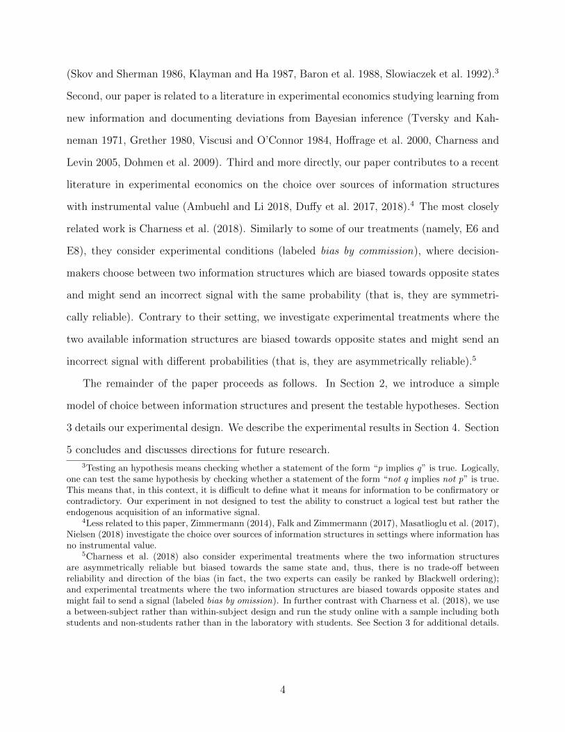
(Skov and Sherman 1986, Klayman and Ha 1987, Baron et al. 1988, Slowiaczek et al. 1992).3

Second, our paper is related to a literature in experimental economics studying learning from

new information and documenting deviations from Bayesian inference (Tversky and Kah-

neman 1971, Grether 1980, Viscusi and O’Connor 1984, Hoffrage et al. 2000, Charness and

Levin 2005, Dohmen et al. 2009). Third and more directly, our paper contributes to a recent

literature in experimental economics on the choice over sources of information structures

with instrumental value (Ambuehl and Li 2018, Duffy et al. 2017, 2018).4 The most closely

related work is Charness et al. (2018). Similarly to some of our treatments (namely, E6 and

E8), they consider experimental conditions (labeled bias by commission), where decision-

makers choose between two information structures which are biased towards opposite states

and might send an incorrect signal with the same probability (that is, they are symmetri-

cally reliable). Contrary to their setting, we investigate experimental treatments where the

two available information structures are biased towards opposite states and might send an

incorrect signal with different probabilities (that is, they are asymmetrically reliable).5

The remainder of the paper proceeds as follows. In Section 2, we introduce a simple

model of choice between information structures and present the testable hypotheses. Section

3 details our experimental design. We describe the experimental results in Section 4. Section

5 concludes and discusses directions for future research.

3Testing an hypothesis means checking whether a statement of the form “p implies q” is true. Logically,one can test the same hypothesis by checking whether a statement of the form “not q implies not p” is true.This means that, in this context, it is difficult to define what it means for information to be confirmatory orcontradictory. Our experiment in not designed to test the ability to construct a logical test but rather theendogenous acquisition of an informative signal.

4Less related to this paper, Zimmermann (2014), Falk and Zimmermann (2017), Masatlioglu et al. (2017),Nielsen (2018) investigate the choice over sources of information structures in settings where information hasno instrumental value.

5Charness et al. (2018) also consider experimental treatments where the two information structuresare asymmetrically reliable but biased towards the same state and, thus, there is no trade-off betweenreliability and direction of the bias (in fact, the two experts can easily be ranked by Blackwell ordering);and experimental treatments where the two information structures are biased towards opposite states andmight fail to send a signal (labeled bias by omission). In further contrast with Charness et al. (2018), we usea between-subject rather than within-subject design and run the study online with a sample including bothstudents and non-students rather than in the laboratory with students. See Section 3 for additional details.

4

2 Task and Theoretical Predictions

Assume there is a binary state of the world, θ = {B,R}, and consider a decision maker

(DM) who has to make a guess, a = {B,R}, about the true state. The DM’s payoff depends

both on this guess and on the realized state of the world:

u(a, θ) =

1 if a = θ

0 if a 6= θ

The DM holds a prior belief, π, about the event θ = B. We consider unbalanced prior

beliefs and, without loss of generality, we assume π ∈ (1/2, 1). Before making a guess,

the DM acquires a piece of information from an information structure σ. The information

structure (or source) stochastically maps the state of the world to a signal s = {b, r}, where

s signals the state is S (that is, b signals the state is B and r signals the state is R). The

DM knows ex ante the distribution of signals, ruling out any uncertainty over information

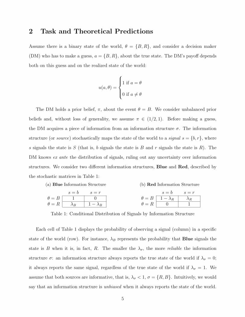
structures. We consider two different information structures, Blue and Red, described by

the stochastic matrices in Table 1:

(a) Blue Information Structure

s = b s = rθ = B 1 0θ = R λB 1− λB

(b) Red Information Structure

s = b s = rθ = B 1− λR λRθ = R 0 1

Table 1: Conditional Distribution of Signals by Information Structure

Each cell of Table 1 displays the probability of observing a signal (column) in a specific

state of the world (row). For instance, λB represents the probability that Blue signals the

state is B when it is, in fact, R. The smaller the λσ, the more reliable the information

structure σ: an information structure always reports the true state of the world if λσ = 0;

it always reports the same signal, regardless of the true state of the world if λσ = 1. We

assume that both sources are informative, that is, λσ < 1, σ = {R,B}. Intuitively, we would

say that an information structure is unbiased when it always reports the state of the world.

5

We exploit this intuition to introduce the following definition of bias:

Definition 1 (Bias)

An information structure σ is biased towards state S if

1. it signals s when the state is S almost surely;

2. it signals s when the state is not S with positive probability.

Using this definition, the two information structures display a “partisan bias”: Blue is

biased towards B and Red is biased towards R. In line with Gentzkow and Shapiro (2006)

we argue this model of distortion can accommodate different real-world interpretations: the

information source may be uninformed about the state and report a default signal; it may

strategically slant its report when the information it holds is against its favorite state; or

its intended signal may inadvertently be distorted. Our simple framework encompasses all

these possibilities, since we do not impose any further condition on the information structure.

What is relevant to us is the information observed by the DM.

The timing of the events is as follows. Given the prior π, the DM chooses whether to

acquire information from Blue or Red. The DM then observes a signal from the chosen

information structure and updates her prior belief. Finally, she submits her guess. The

ensuing payoff is 1 if the guess matches the state of the world, and 0 otherwise.

Our object of analysis is the information acquisition behavior of the DM when faced

with different information sources, and how this varies with her prior belief and the available

sources’ reliability. Note that the only goal of the DM in this framework is to maximize her

expected payoff, which she can do by picking the most informative source and processing its

signal as a Bayesian learner. Indeed, after observing a signal from an information source,

the expected payoff from a guess coincides with the posterior belief this guess matches the

true state of the world. Hence, posterior beliefs fully characterize the optimal choice of the

DM.

6

We characterize the DM’s optimal choice of an information source by backward induction.

First, we investigate the optimal guess for a given signal received by a given source. Second,

we investigate what information source the DM prefers to consult, given the distribution of

signals induced by each information structure and how the DM will use these signals. In

what follows, the notation a?(s, σ) denotes the optimal guess after observing signal s from

information structure σ. Posterior beliefs are denoted by Pr(θ|s, σ). All proofs are reported

in the Appendix.

2.1 Optimal Guess for Given Information Source

Lemma 1 (Optimal Guess if Signal from Blue Source) The DM always follows the

signal received from source Blue, that is, a?(b,Blue) = B and a?(r,Blue) = R.

Lemma 2 (Optimal Guess if Signal from Red Source) The DM always follows a con-

firmatory signal received from source Red, that is, a?(b,Red) = B. The DM follows a con-

tradictory signal received from source Red if and only if the source is sufficiently reliable,

that is, a?(r,Red) = R if λR <1−ππ

and a?(r,Red) = B otherwise.

When she observes a signal confirming her prior from either source, the DM’s posterior belief

that θ = B is strictly greater than her prior. This means that, in this case, the DM sticks

with her prior belief and guesses accordingly. Receiving a signal which disagrees with the

source bias — that is, receiving signal b (r) from the Red (Blue) information structure —

is fully revealing: the DM learns the state with certainty, independently of her prior beliefs

and the information source reliability. Finally, when she observes signal r from Red, the

DM’s posterior belief that θ = B is strictly smaller than her prior. In this case, the optimal

guess depends on the model parameters: if Red is sufficiently reliable (i.e., λR is sufficiently

small), it is optimal to follow its signal. Otherwise, the DM is better off ignoring the signal

altogether and sticking with the guess induced by her prior belief. The relative size of λR

must be gauged against the prior belief: the larger the prior in favor of B, the higher the

7

reliability of Red required by the DM to follow an r signal from this source.

2.2 Optimal Choice of Information Source

We now move a step backward in the DM’s problem and consider her decision about what

source to acquire information from. First, consider the expected payoff from consulting the

source biased in favor of the prior, that is, Blue. As discussed above, the DM follows any sig-

nal received from this source. Thus, her posterior belief that she is making the correct guess is

Pr(θ = R|r,Blue) = 1 following a contradictory signal; and Pr(θ = B|b,Blue) = ππ+(1−π)λB

following a confirmatory signal. Weighing these posterior beliefs with the unconditional

distribution of signals by this source, we get the following expected payoff:

Lemma 3 (Expected Utility from Blue Source) E[Blue] = 1 − (1 − π)λB ∈ [π, 1] is

increasing in π and decreasing in λB.

Accessing this source always improves the confidence the DM has in her guess with respect

to the decision she would made without collecting any additional information. The benefit

is increasing in the likelihood its bias is in line with the true state and with its reliability.

Consider now the expected payoff from consulting the source biased against the prior, that

is, Red. As discussed above, when this source is not sufficiently reliable — that is, λR ≥ 1−ππ

— the DM guesses B regardless of the signal. Thus, in this case, the expected payoff from

consulting this information source is equal to the expected payoff from not consulting any

source and deciding on the basis of the prior belief. On the other hand, when λR < 1−ππ

,

the DM follows any signal received from Red. In this case, her posterior belief that she is

making the correct guess is Pr(θ = R|r,Red) = 1−ππλR+(1−π) following a contradictory signal;

and Pr(θ = B|b,Red) = 1 following a confirmatory signal. Weighing these posterior beliefs

with the unconditional distribution of signals by this source, we get the following expected

payoff:

8

Lemma 4 (Expected Utility from Red Source) If λR ≥ 1−ππ

, E[Red] = π. If, instead,

λR <1−ππ

, E[Red] = 1− πλR ∈ [π, 1], decreasing in π and in λR.

Accessing this source improves the confidence the DM has in her guess only when it is

sufficiently reliable. In this case, the benefit is increasing in the likelihood its bias is in line

with the true state and with its reliability.

Since consulting the source biased in favor of the prior is always informative, that is,

E[Blue] > π, the DM is better off consulting Blue when λR ≥ 1−ππ

. When λR <1−ππ

, both

sources are informative and the choice involves a trade off. Intuitively, the DM chooses the

information structure with the smallest probability of misleading signals. If the DM has a

perfectly balanced prior, that is, π = 1/2, choosing Red over Blue reduces to λR < λB.

When the prior is unbalanced, that is, π > 1/2, the DM has an incentive to choose the

information structure which is biased towards the prior. She prefers to observe a signal

from Red only when this information source is sufficiently more reliable than the other.

Proposition 1 summarizes this discussion and characterizes this threshold:

Proposition 1 (Optimal Source) The DM consults Red if and only if λR <1−ππλB and

Blue otherwise.

2.3 Summary of Testable Hypotheses

Below, we summarize the testable hypotheses that we set out to investigate empirically.

On Information Acquisition

H1 When information sources are equally reliable, it is optimal to seek confirming infor-

mation, that is, to acquire information from the source biased towards the prior.

H2 When the source biased against the prior is more reliable, it is optimal to acquire

information from the more reliable source (even if biased against the prior) if the prior

9

is mildly unbalanced; it is optimal to acquire information from the source biased towards

the prior (even if less reliable) if the prior is strongly unbalanced.

On Information Processing

H3 It is always optimal to follow information from the source biased towards the prior.

H4 It is always optimal to follow confirming information from the source biased against

the prior. Contradictory information from the source biased against the prior should

be followed when the prior is mildly unbalanced and ignored when the prior is strongly

unbalanced.

3 Experimental Design

The experiment was conducted online on Prolific, a crowdsourcing platform for academic

research. Subjects were recruited from the Prolific database of participants and screened

by their characteristics: only American citizens currently residing in the U.S. whose first

language was English were eligible for participation. A total of 201 subjects took part

in the experiment, and no subject was able to sit for the experiment twice. While not

representative of the American population, our sample is more representative than traditional

samples composed of undergraduate students at elite universities.6 The use of web-based

experiments is relatively novel in experimental economics. While this methodology requires

additional precautions in the design and in the instructions in order to ensure continuous

attention7, research suggests test results are in line with those obtained in more controlled

6In our sample, age ranged between 19 and 75 years old, with an average age of 33.4 (N = 192 out of 201participants); 51% of participants were women (N = 198); 28.4% of participants were students (N = 197);56.3% of participants were full time workers (N = 192); 77% of participants had at least some collegeeducation (N = 196); 75.8% of participants were caucasian; the median personal income was in the $40k-$50k bracket (N = 169); the median household income was in the $65k-$75k bracket (N = 157); 50.8% ofparticipants were Democrat (with 19.8% being a Republican and 29.5% being an Independent, N = 193).These statistics are based on self-declarations collected by Prolific.

7The rest of this Section details how we achieved this.

10

environments such as laboratories (?, Snowberg and Yariv 2018). Instructions and sample

screens are reported in Appendix C.8

Setup. The task builds on the classic urn paradigm, which has been extensively used in

the experimental literature since Anderson and Holt (1997). Subjects are first introduced

to the problem of guessing the color of a ball (either red or blue) randomly drawn from

a jar containing only blue and red balls, for a total of 10 balls. One of our experimental

manipulations is participants’ prior belief (π) about the state of the world. We provide

participants with a prior belief on the color of the extracted ball by displaying information

on the distribution of the balls in the jar.

Next, we model the information structures as imperfectly informed “experts”. Before

making their guess, participants have to consult either the Blue Expert or the Red Expert,

randomly extracted from two population of experts (the Red population and the Blue pop-

ulation). In each population, a certain fraction of experts is informed about the true color

of the extracted ball and issues a report revealing such true color. The complementary frac-

tion of experts is uninformed about the color of the extracted ball and always issues the

same report. In particular, a random Blue Expert is informed with probability (1 − λB)

and uninformed with probability λB. When uninformed, a Blue Expert always reports the

color of the extracted ball is blue. Analogously, picking randomly a Red Expert implies he is

informed with probability (1− λR) and uninformed with probability λR. When uninformed,

the expert always reports the color of the ball is red. Both experts can be consulted for free,

but participants are forced to choose only one of them.

Choosing the expert prompts participants to the following screen, where we use the

strategy method and elicit a subject’s guess about the color of the ball conditional on the

expert’s signal. On the same screen, we elicit a subject’s confidence in each of these two

conditional guesses, on a scale between 0 and 100.9 Once these choices have been recorded,

8The user interface was programmed with oTree (Chen et al. 2016).9As detailed in the Instructions available in Appendix C, we elicit confidence with the following question:

“On a scale from 0 to 100, how confident are you about this guess? For example, 0 means that you think it

11

participants proceed to the final screen where they see the expert’s signal, their relevant

choice given the signal, the color of the extracted ball, and their payoff.

Instructions are displayed in the first screens of the experiment and followed by three

multiple-choice questions to verify participants understand the details of the experiment.

After answering each of these questions, subjects see a commented feedback page with the

correct answers and a further explanation of the reasoning leading to the correct answer.10

Each page of the instructions is timed, so that participants must spend no less than a specified

amount of time on each page, ranging from 30 to 60 seconds.

Rounds. The discussion above describes one round of the experiment. The experiment

consists in a sequence of 5 rounds and it lasts around 10 minutes. In each round, the

computer draws the true state of the world and the messages sent by the two experts from

the same distributions and independently from any past action or outcome. Playing multiple

rounds, subjects familiarize with the structure of the experiment and have room for learning.

We opted for a limited number of rounds for two reasons. First, we wanted participants

to pay due attention to the instructions and forced them to spend no less than a specified

amount of time reading them. Increasing the number of rounds may lead participants to skim

quickly through the instructions in order to have more time to formulate each subsequent

(remunerated) choice. Second, given the online implementation of the experiment, we wanted

to avoid boredom: keeping the number of rounds at a minimum favors attention.

Choices. In each round, we are eliciting five choices from each participant: the expert to

consult, the guess on the color of the ball for each possible signal from the chosen expert,

and the confidence level surrounding these guesses. The strategy method allows us to record

information also for unlikely events. Moreover, we use confidence statements to construct

is just as likely that you are right or wrong and 100 means you are sure your guess is correct.”1047% of participants (94 out 201) answered all three comprehension questions correctly; 87% (175 out

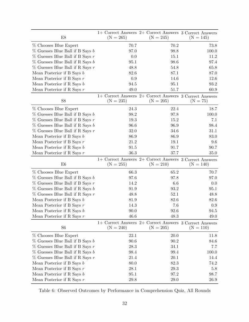
of 201) answered at least two questions correctly; and 99% (199 out of 201) answered at least one questioncorrectly. Results are qualitatively unchanged if we consider only subjects who answered correctly 1, 2 or 3comprehension questions. Table 6 in Appendix B reports observed behavior in the subsamples determinedby the number of questions answered correctly in the comprehension quiz.

12

a measure of observed posterior beliefs, which we exploit to test for systematic biases in

distinct treatments.11 We do not incentivize confidence statements for two reasons. First,

given the experiment was administered online, we deemed as particularly important to keep

the tasks simple and the total duration short (below 20 minutes). Explaining carefully

a Binary Scoring Rule and guaranteeing a full understanding of the underlying incentives

would have required some additional time, possibly more than the duration of the main task,

increasing attrition and reducing the quality of decisions throughout the whole experiment.

Second, incentivizing the elicitation of posterior beliefs (either with a Binary Scoring Rule or

asking for the closest guess to the posterior belief held by a statistician, as in Charness and

Dave 2017) could potentially interfere with the fundamental incentive to choose the most

informative expert, as it gives an incentive to choose informational sources which are more

likely to induce degenerate posterior beliefs. At the same time, in the instructions, we stress

the importance of revealing truthful confidence assessments.

Payoffs. On top of earning a fixed amount of $1 for taking part in the experiment, subjects

are remunerated for guessing the color of the ball. In particular, they earn $1 if their

guess matches the color of the drawn ball, $0 otherwise. At the beginning of the experiment

participants are instructed they will play multiple rounds, but only a randomly chosen round

will be selected to determine the bonus payment. As discussed above, we do not incentivize

the elicitation of a subject’s confidence in his/her guess.

Treatments. We employ a between-subjects design, where we manipulate the prior belief

that the ball drawn from the jar is blue, π, and the relative reliability of the two experts,

(λR, λB). We consider both a mildly and a strongly unbalanced prior, respectively π =

0.6 and π = 0.8. Regarding the probability that experts garble their signals, we consider

the case where Blue and Red Experts are equally reliable, (λR, λB) = (0.5, 0.5), and the case

11We mapped a confidence of 0 — that is, “I think it is just as likely that I am right or wrong” — to aposterior belief of 0.5 (i.e., indifference between guessing blue and guessing red) and a confidence of 100 —that is, “I think I am sure my guess is correct” — to a posterior of 1 (i.e. almost certainty in the choice).Intermediate levels of confidence were mapped proportionally to intermediate posteriors between 0.5 and 1.

13

λB

λR

1

1

0

λR = 0.5

λB = 0.5

1−ππ

E8

S8

(a) π = 0.8

λB

λR

1

1

0

λR = 0.5

λB = 0.5

1−ππ

E6

S6

(b) π = 0.6

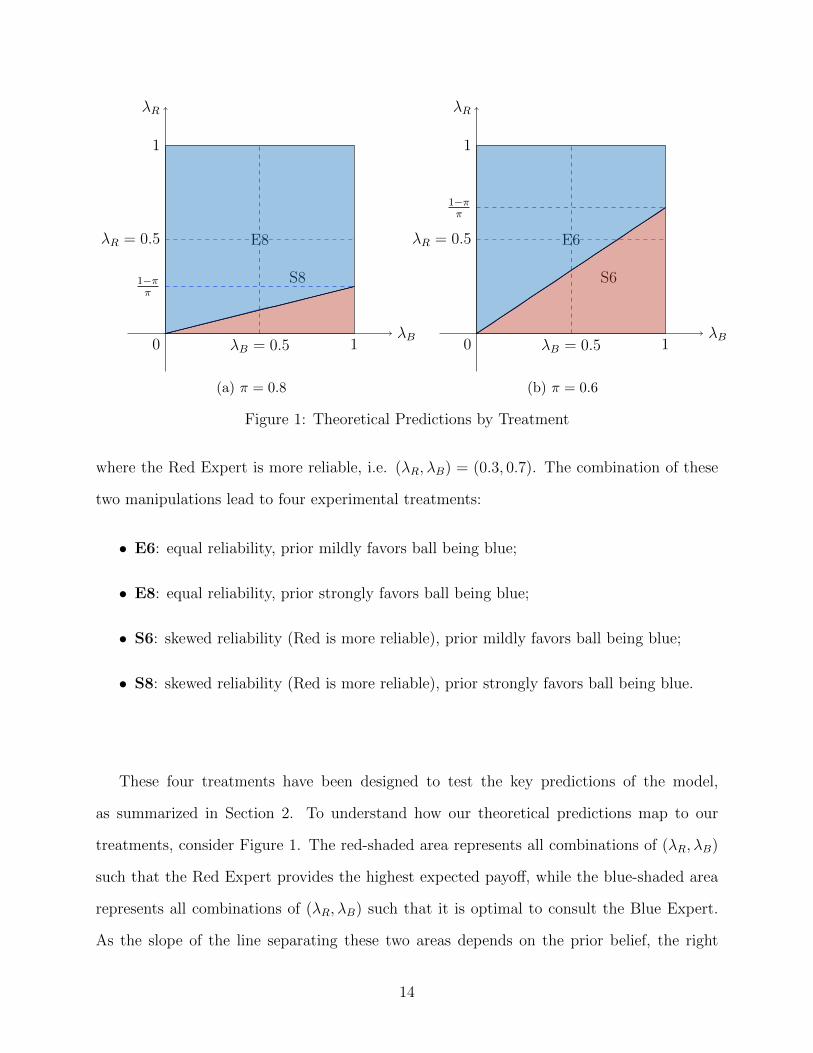
Figure 1: Theoretical Predictions by Treatment

where the Red Expert is more reliable, i.e. (λR, λB) = (0.3, 0.7). The combination of these

two manipulations lead to four experimental treatments:

• E6: equal reliability, prior mildly favors ball being blue;

• E8: equal reliability, prior strongly favors ball being blue;

• S6: skewed reliability (Red is more reliable), prior mildly favors ball being blue;

• S8: skewed reliability (Red is more reliable), prior strongly favors ball being blue.

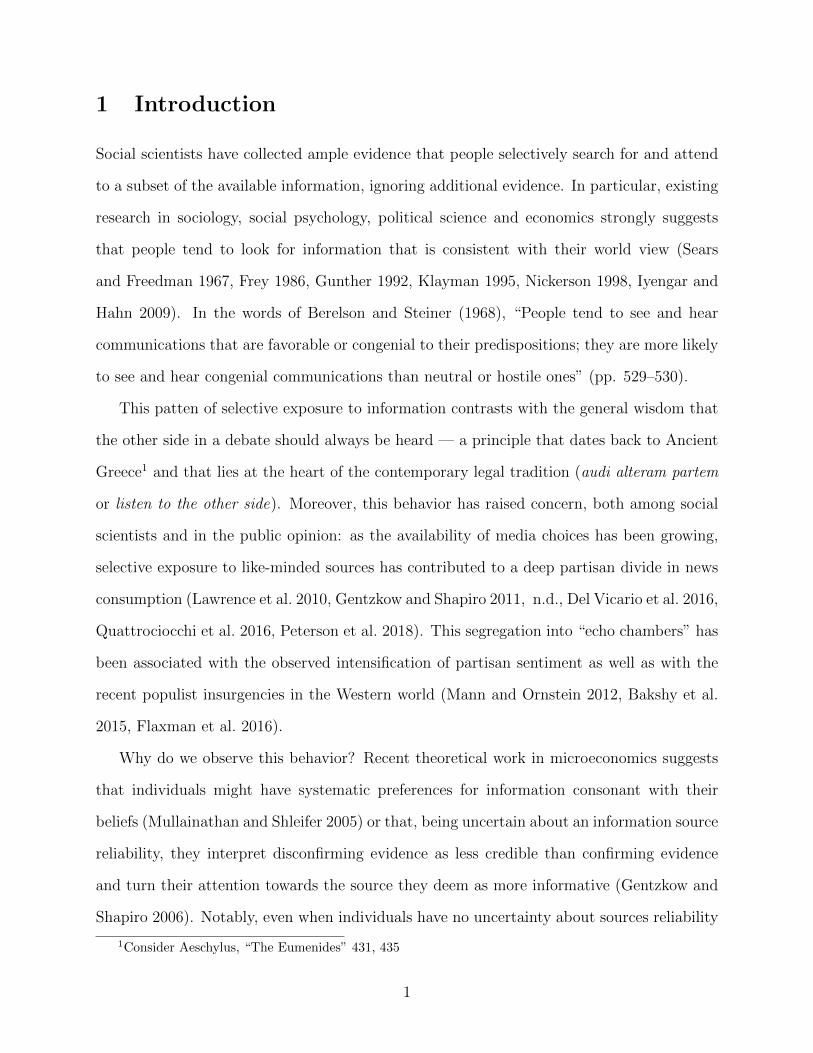
These four treatments have been designed to test the key predictions of the model,

as summarized in Section 2. To understand how our theoretical predictions map to our

treatments, consider Figure 1. The red-shaded area represents all combinations of (λR, λB)

such that the Red Expert provides the highest expected payoff, while the blue-shaded area

represents all combinations of (λR, λB) such that it is optimal to consult the Blue Expert.

As the slope of the line separating these two areas depends on the prior belief, the right

14

panel is for the mildly unbalanced prior and the left panel for the strongly unbalanced prior.

Only when the Red Expert is more reliable and when the prior is mildly unbalanced — that

is, in treatment S6 — it is optimal to consult the contrarian expert. In all other treatments,

it is optimal to consult the supportive expert. Treatments E8 and E6 allow us to test a

crucial prediction of the model, namely that when experts are equally reliable and the prior

is unbalanced subjects prefer to get advice from the supportive expert (H1). Treatments S8

and S6 allows us to test the effect of the prior on the incentives to consult the contrarian

expert (H2). We can restate the predictions from Section 2.3 in terms of our treatments:

H1 Subjects acquire information from the Blue Expert in both E6 and E8.

H2 Subjects acquire information from the Red Expert in S6, from the Blue Expert in S8.

H3 Subjects always follow signals by the Blue Expert.

H4 Subjects always follow Blue signals by the Red Expert. Subjects follow Red signals by

the Red Expert in E6 and S6 but ignore them in E8 and S8.

4 Experimental Results

4.1 Information Acquisition

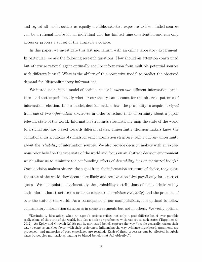
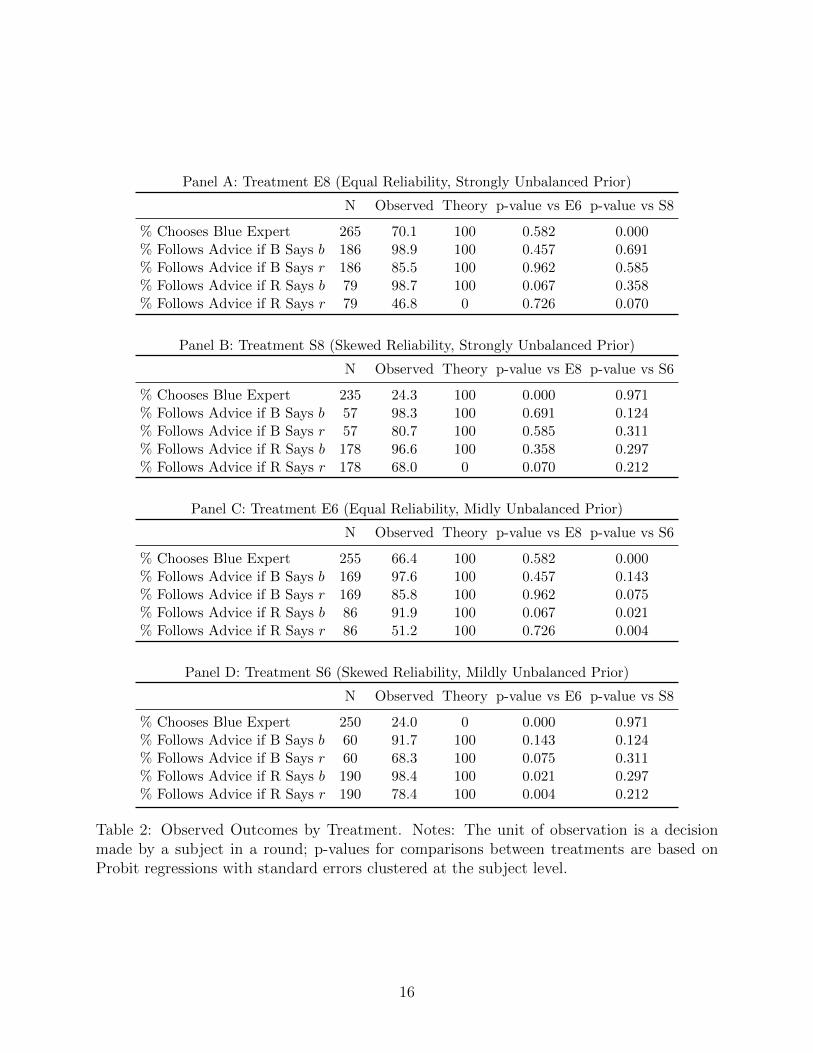
Table 2 and Figure 2 show the percentage of decisions where subjects consulted the Blue Ex-

pert — that is, the expert biased in favor of the prior — disaggregated by treatment. When

information sources are equally reliable, this happens in 66.4% of decisions with mildly un-

balanced priors (treatment E6) and in 70.1% of decisions with strongly unbalanced priors

(treatment E8). These proportions are statistically different from 50%, according to one-

sample tests of proportions (p-values < 0.001). This behavior is in line with hypothesis H1,

as the Blue Expert is always the more informative in these environments. When the informa-

tion source biased against the prior (i.e., the Red Expert) is more reliable, the Blue Expert

15

Panel A: Treatment E8 (Equal Reliability, Strongly Unbalanced Prior)

N Observed Theory p-value vs E6 p-value vs S8

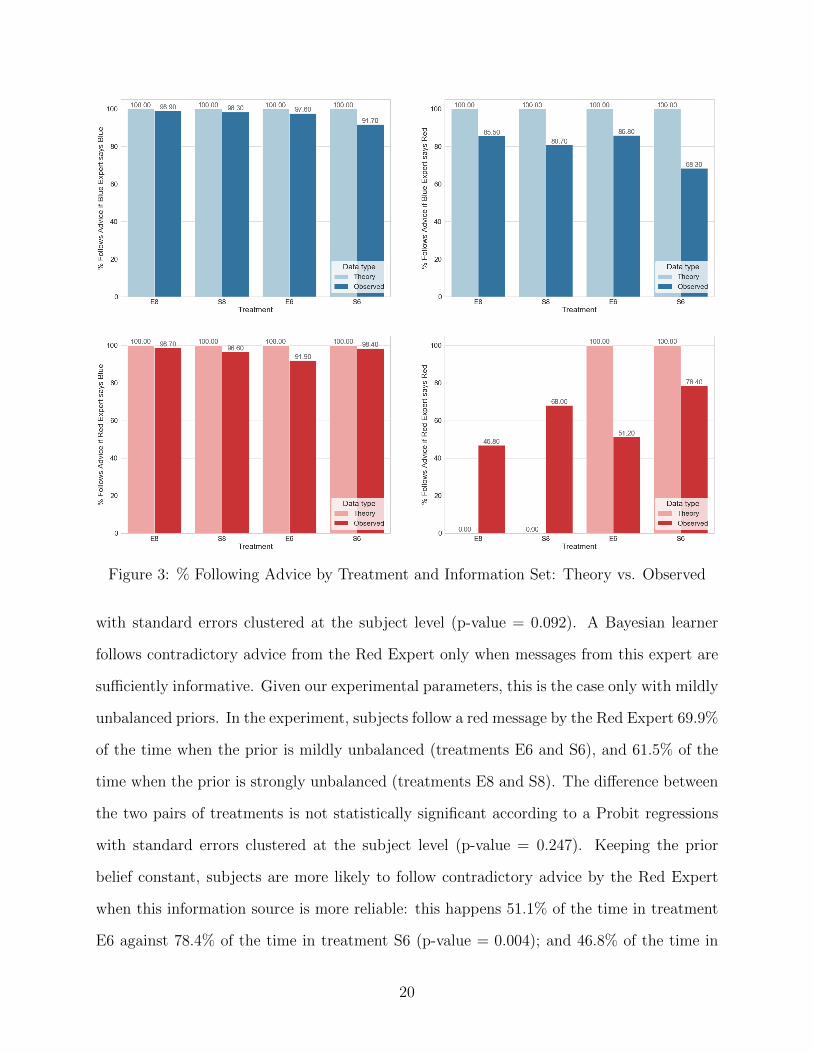
% Chooses Blue Expert 265 70.1 100 0.582 0.000% Follows Advice if B Says b 186 98.9 100 0.457 0.691% Follows Advice if B Says r 186 85.5 100 0.962 0.585% Follows Advice if R Says b 79 98.7 100 0.067 0.358% Follows Advice if R Says r 79 46.8 0 0.726 0.070

Panel B: Treatment S8 (Skewed Reliability, Strongly Unbalanced Prior)



Panel C: Treatment E6 (Equal Reliability, Midly Unbalanced Prior)



Panel D: Treatment S6 (Skewed Reliability, Mildly Unbalanced Prior)



Table 2: Observed Outcomes by Treatment. Notes: The unit of observation is a decisionmade by a subject in a round; p-values for comparisons between treatments are based onProbit regressions with standard errors clustered at the subject level.

16

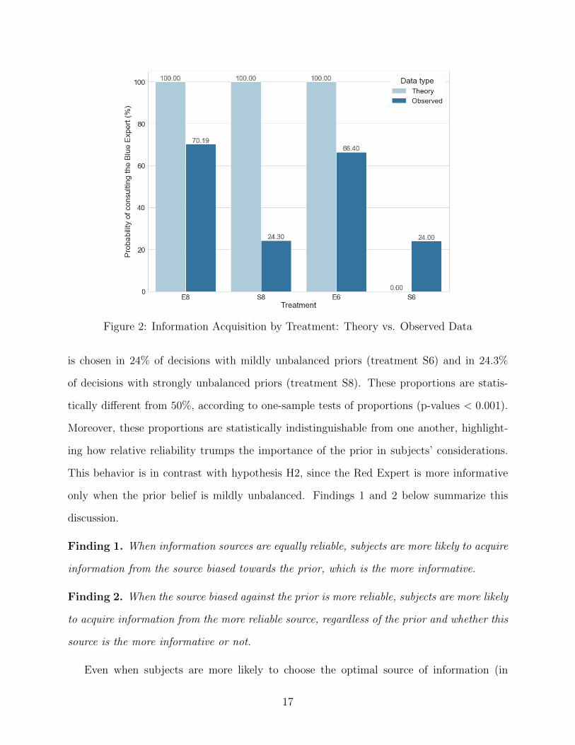
Figure 2: Information Acquisition by Treatment: Theory vs. Observed Data

is chosen in 24% of decisions with mildly unbalanced priors (treatment S6) and in 24.3%

of decisions with strongly unbalanced priors (treatment S8). These proportions are statis-

tically different from 50%, according to one-sample tests of proportions (p-values < 0.001).

Moreover, these proportions are statistically indistinguishable from one another, highlight-

ing how relative reliability trumps the importance of the prior in subjects’ considerations.

This behavior is in contrast with hypothesis H2, since the Red Expert is more informative

only when the prior belief is mildly unbalanced. Findings 1 and 2 below summarize this

discussion.

Finding 1. When information sources are equally reliable, subjects are more likely to acquire

information from the source biased towards the prior, which is the more informative.

Finding 2. When the source biased against the prior is more reliable, subjects are more likely

to acquire information from the more reliable source, regardless of the prior and whether this

source is the more informative or not.

Even when subjects are more likely to choose the optimal source of information (in

17

treatments E6, E8 and S6), they are prone to mistakes: when information sources are equally

reliable, they listen too often to the expert biased against the prior (33.6% of decisions in

E6 and 28.8% of decisions in E8); when the Red Expert is more reliable and the uncertainty

on the state is sufficiently strong, they listen too often to the expert biased in favor of the

prior (24% of decisions in S6). Mistakes are, of course, even more frequent when subjects

are more likely to consult the less informative expert (in treatment S8, when this happens

in 75.5% of decisions).

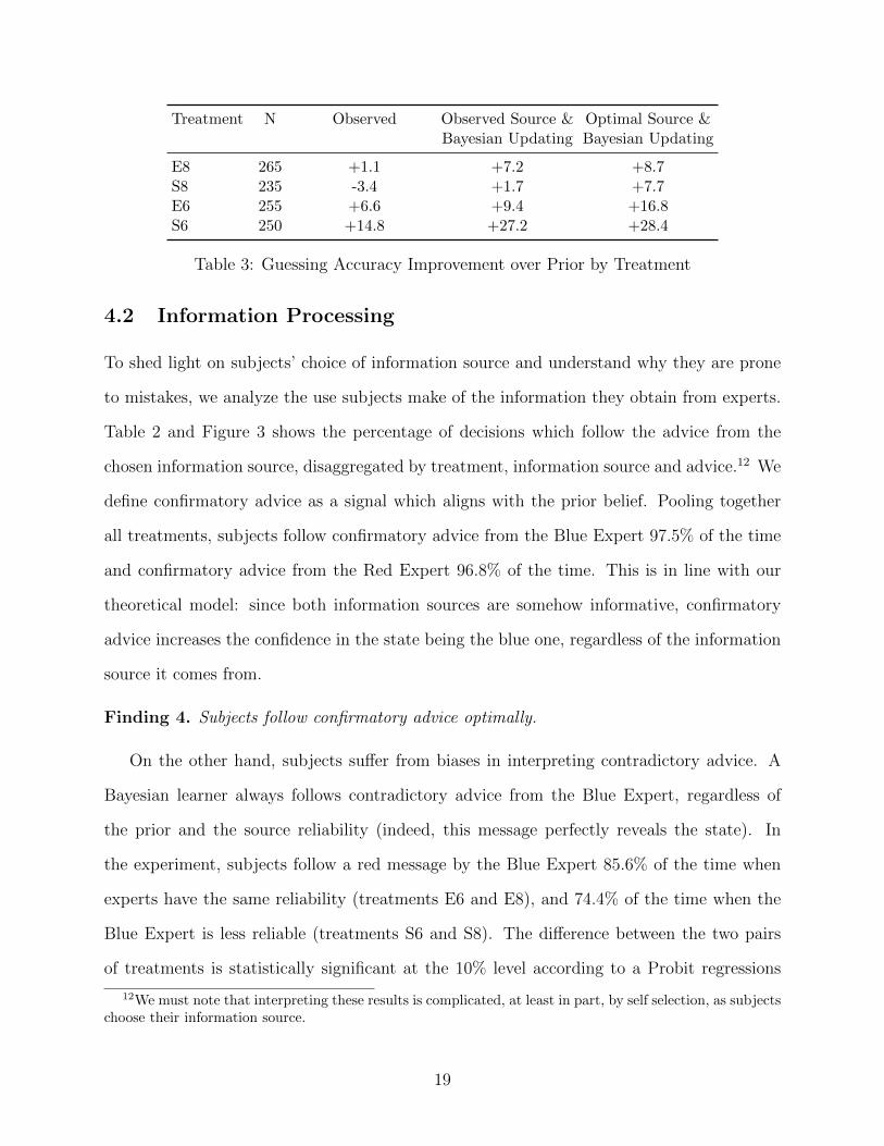
Importantly, these mistake rates come at a cost in terms of accuracy in guessing the

state. To show this, Table 3 reports the average guessing accuracy improvement over the

prior — that is, the change in the probability of correctly guessing the state relative to sim-

ply following the prior — disaggregated by treatment. We compare the observed guessing

accuracy improvement with two benchmarks: the guessing accuracy improvement by hypo-

thetical subjects who choose the same information structure as actual subjects but process

the information as Bayesian learners; and the guessing accuracy improvement by hypothet-

ical subjects who choose the optimal information structure and process the information as

Bayesian learners. The results show that subjects improve guessing accuracy less than they

could in all treatments. Indeed, when experts have asymmetric reliability and the prior is

strongly unbalanced, subjects actually make worse guesses than they would simply follow-

ing their priors. In part, this is due to subjects making sub-optimal use of the information

provided by experts (regardless of whether the chosen information structure was optimal or

not): the improvement in average accuracy that could be obtained without changing infor-

mation source but adopting Bayesian inference ranges between 2.8% (in treatment E6) to

12.4% (in treatment S6). At the same time, choosing a suboptimal information structure

also has a cost in terms of guessing accuracy, especially in treatments S8 and E6.

Finding 3. In all treatments, subjects frequently acquire information from the less informa-

tive source and this leads to sub-optimal learning.

18

Treatment N Observed Observed Source & Optimal Source &Bayesian Updating Bayesian Updating

E8 265 +1.1 +7.2 +8.7S8 235 -3.4 +1.7 +7.7E6 255 +6.6 +9.4 +16.8S6 250 +14.8 +27.2 +28.4

Table 3: Guessing Accuracy Improvement over Prior by Treatment

4.2 Information Processing

To shed light on subjects’ choice of information source and understand why they are prone

to mistakes, we analyze the use subjects make of the information they obtain from experts.

Table 2 and Figure 3 shows the percentage of decisions which follow the advice from the

chosen information source, disaggregated by treatment, information source and advice.12 We

define confirmatory advice as a signal which aligns with the prior belief. Pooling together

all treatments, subjects follow confirmatory advice from the Blue Expert 97.5% of the time

and confirmatory advice from the Red Expert 96.8% of the time. This is in line with our

theoretical model: since both information sources are somehow informative, confirmatory

advice increases the confidence in the state being the blue one, regardless of the information

source it comes from.

Finding 4. Subjects follow confirmatory advice optimally.

On the other hand, subjects suffer from biases in interpreting contradictory advice. A

Bayesian learner always follows contradictory advice from the Blue Expert, regardless of

the prior and the source reliability (indeed, this message perfectly reveals the state). In

the experiment, subjects follow a red message by the Blue Expert 85.6% of the time when

experts have the same reliability (treatments E6 and E8), and 74.4% of the time when the

Blue Expert is less reliable (treatments S6 and S8). The difference between the two pairs

of treatments is statistically significant at the 10% level according to a Probit regressions

12We must note that interpreting these results is complicated, at least in part, by self selection, as subjectschoose their information source.

19

Figure 3: % Following Advice by Treatment and Information Set: Theory vs. Observed

with standard errors clustered at the subject level (p-value = 0.092). A Bayesian learner

follows contradictory advice from the Red Expert only when messages from this expert are

sufficiently informative. Given our experimental parameters, this is the case only with mildly

unbalanced priors. In the experiment, subjects follow a red message by the Red Expert 69.9%

of the time when the prior is mildly unbalanced (treatments E6 and S6), and 61.5% of the

time when the prior is strongly unbalanced (treatments E8 and S8). The difference between

the two pairs of treatments is not statistically significant according to a Probit regressions

with standard errors clustered at the subject level (p-value = 0.247). Keeping the prior

belief constant, subjects are more likely to follow contradictory advice by the Red Expert

when this information source is more reliable: this happens 51.1% of the time in treatment

E6 against 78.4% of the time in treatment S6 (p-value = 0.004); and 46.8% of the time in

20

treatment E8 against 68% of the time in treatment S8 (p-value = 0.070). Theoretically, even

if increasing the Red Expert’s reliability does increase the sensitivity of posterior beliefs to

its advice, contradictory advice by the Red Expert should affect the optimal guess only when

the initial belief is not too strong (and for both levels of reliability).

Finding 5. Subjects follow contradictory advice sub-optimally: they are excessively skeptic

of contradictory advice by the expert biased towards the prior and excessively trusting of

contradictory advice by the expert biased against the prior.

To understand why subjects’ decision-making after receiving a contradictory signal is

different from the Bayesian benchmark, we map the (non-incentivized) confidence levels in

the guess to posterior beliefs on the state of the world and analyze them. We follow Charness

et al. (2018) and define responsiveness to information as follows:

αs =ps − p0pBays − p0

where ps is the observed posterior belief, p0 is the prior belief and pBay is the posterior belief

held by a Bayesian learner with the same information. Note that αs = 1 corresponds to

Bayesian updating, αs < 1 corresponds to under-responsiveness and αs > 1 corresponds to

over-responsiveness. We calculate αs for each decision and show the average by treatment

and information set in Table 4.

Table 4 shows that subjects’ posterior beliefs are statistically indistinguishable from those

of Bayesian learners when advice is in line with the source bias and the prior is more fa-

vorable to this bias: average responsiveness is not statistically different from 1 when the

prior is strongly unbalanced and the Blue Expert suggests blue; and when the prior is mildly

unbalanced and the Red Expert suggests red. At the same time, subjects are too trusting

of advice in line with an expert’s bias when the prior is less favorable to this bias: subjects

are excessively responsive to a blue message by the Blue Expert when the prior is mildly

unbalanced (average responsiveness being 1.5 in E6 and 2.5 in S6); and excessively respon-

21

Panel A: Treatment E8 (Equal Reliability, Strongly Unbalanced Prior)

N Observed Theory p-value

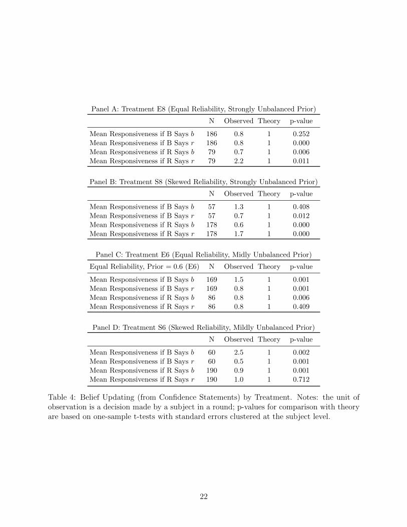
Mean Responsiveness if B Says b 186 0.8 1 0.252Mean Responsiveness if B Says r 186 0.8 1 0.000Mean Responsiveness if R Says b 79 0.7 1 0.006Mean Responsiveness if R Says r 79 2.2 1 0.011

Panel B: Treatment S8 (Skewed Reliability, Strongly Unbalanced Prior)



Panel C: Treatment E6 (Equal Reliability, Midly Unbalanced Prior)

Equal Reliability, Prior = 0.6 (E6) N Observed Theory p-value


Panel D: Treatment S6 (Skewed Reliability, Mildly Unbalanced Prior)



Table 4: Belief Updating (from Confidence Statements) by Treatment. Notes: the unit ofobservation is a decision made by a subject in a round; p-values for comparison with theoryare based on one-sample t-tests with standard errors clustered at the subject level.

22

sive to a red message by the Red Expert when the prior is strongly unbalanced (average

responsiveness being 2.2 in E8 and 1.7 in S8). Moreover, subjects are always too skeptic

of advice in conflict with an expert’s bias (which, in fact, perfectly reveals the state of the

world): the average responsiveness in these cases ranges from 0.5 (in treatment S6 when

the Blue Experts says red) to 0.9 (in treatment S6 when the Red Expert says blue) and is

statistically different from 1 for all treatments and information sets. Finding 6 summarizes

this discussion.

Finding 6. Subjects are insufficiently responsive to information misaligned with a source

bias and excessively responsive to information aligned with a source bias.

5 Conclusions

This paper formalized a model of selective exposure based on Bayesian updating, and tested

its predictions through an online experiment. We ask two research questions: when is it

rational to seek (dis)confirmatory information? Do experimental subjects behave according

to rationality or do we need to impose additional structures? We modeled the problem

of selective exposure to information as a choice between experts with different reliability.

Overall, our experiment suggests that explaining selective exposure to information sources

with Bayesian inference has some limitations: in line with Bayesian learning, we do observe

confirmatory patterns in the selection of information source when experts are equally reliable;

at the same time, these trends switch to dis-confirmatory attitudes as soon as the expert

biased against the prior becomes more informative, with no role for the strength of prior

beliefs. We see many possible directions for future research: while we study the simplest

possible setup to investigate selective exposure to information sources, it would be interesting

to investigate more complex environments where decision-makers have the opportunity to

collect multiple pieces of information from experts, or must pay a (possibly heterogeneous)

price to receive messages from an information structure.

23

References

Ambuehl, Sandro and Shengwu Li, “Belief Updating and the Demand for Information,”Games and Economic Behavior, 2018, 109, 21–39.

Anderson, Lisa R and Charles A Holt, “Information Cascades in the Laboratory,”American Economic Review, 1997, 87 (5), 847–862.

Bakshy, Eytan, Solomon Messing, and Lada A Adamic, “Exposure to ideologicallydiverse news and opinion on Facebook,” Science, 2015, 348 (6239), 1130–1132.

Baron, Jonathan, Jane Beattie, and John C Hershey, “Heuristics and Biases in Di-agnostic Reasoning II: Congruence, Information, and Certainty,” Organizational Behaviorand Human Decision Processes, 1988, 42 (1), 88–110.

Berelson, Bernard and Gary A Steiner, Human Behavior: An Inventory of ScientificFindings, Springer, 1968.

Charness, Gary and Chetan Dave, “Confirmation Bias with Motivated Beliefs,” Gamesand Economic Behavior, 2017, 104, 1–23.

and Dan Levin, “When Optimal Choices Feel Wrong: A Laboratory Study of BayesianUpdating, Complexity, and Affect,” American Economic Review, 2005, 95 (4), 1300–1309.

, Ryan Oprea, and Sevgi Yuksel, “How Do People Choose between Biased InformationSources? Evidence from a Laboratory Experiment,” Unpublished Manuscript, 2018.

Chen, Daniel L, Martin Schonger, and Chris Wickens, “oTree: An Open-SourcePlatform for Laboratory, Online, and Field Experiments,” Journal of Behavioral and Ex-perimental Finance, 2016, 9, 88–97.

Dohmen, Thomas J, Armin Falk, David Huffman, Felix Marklein, and UweSunde, “The Non-Use of Bayes Rule: Representative Evidence on Bounded Rationality,”Unpublished Manuscript, 2009.

Duffy, John, Ed Hopkins, and Tatiana Kornienko, “Lone Wolf or Herd Animal?Information Choice and Social Learning,” Unpublished Manuscript, 2017.

, , , and Mingye Ma, “Information Choice in a Social Learning Experiment,”Unpublished Manuscipt, 2018.

Epley, Nicholas and Thomas Gilovich, “The Mechanics of Motivated Reasoning,” TheJournal of Economic Perspectives, 2016, 30 (3), 133–140.

Falk, Armin and Florian Zimmermann, “Beliefs and Utility: Experimental Evidenceon Preferences for Information,” Unpublished Manuscript, 2017.

24

Flaxman, Seth, Sharad Goel, and Justin M Rao, “Filter Bubbles, Echo Chambers,and Online News Consumption,” Public Opinion Quarterly, 2016, 80 (S1), 298–320.

Frey, Dieter, “Recent Research on Selective Exposure to Information,” Advances in Exper-imental Social Psychology, 1986, 19, 41–80.

Gentzkow, Matthew and Jesse M Shapiro, “Media Bias and Reputation,” Journal ofPolitical Economy, 2006, 114 (2), 280–316.

and , “Ideological Segregation Online and Offline,” Quarterly Journal of Economics,2011, 126 (4), 1799–1839.

Grether, David M, “Bayes Rule as a Descriptive Model: The Representativeness Heuris-tic,” Quarterly Journal of Economics, 1980, 95 (3), 537–557.

Gunther, Albert C, “Biased press or biased public? Attitudes toward media coverage ofsocial groups,” Public Opinion Quarterly, 1992, 56 (2), 147–167.

Hoffrage, Ulrich, Samuel Lindsey, Ralph Hertwig, and Gerd Gigerenzer, “Com-municating Statistical Information,” Science, 2000, 290 (5500), 2261–2262.

Iyengar, Shanto and Kyu S Hahn, “Red Media, Blue Media: Evidence of IdeologicalSelectivity in Media Use,” Journal of Communication, 2009, 59 (1), 19–39.

Klayman, Joshua, “Varieties of Confirmation Bias,” Psychology of Learning and Motiva-tion, 1995, 32, 385–418.

and Young-Won Ha, “Confirmation, Disconfirmation, and Information in HypothesisTesting.,” Psychological Review, 1987, 94 (2), 211.

Lawrence, Eric, John Sides, and Henry Farrell, “Self-Segregation or Deliberation?Blog Readership, Participation, and Polarization in American Politics,” Perspectives onPolitics, 2010, 8 (1), 141–157.

Mann, Thomas E. and Norman J. Ornstein, It’s Even Worse Than It Looks: Howthe American Constitutional System Collided with the New Politics of Extremism, BasicBooks, New York, NY, 2012.

Masatlioglu, Yusufcan, A Yesim Orhun, and Collin Raymond, “Intrinsic Informa-tion Preferences and Skewness,” Unpublished Manuscript, 2017.

Mullainathan, Sendhil and Andrei Shleifer, “The Market for News,” American Eco-nomic Review, 2005, 95 (4), 1031–1053.

Nickerson, Raymond S, “Confirmation Bias: A Ubiquitous Phenomenon in Many Guises,”Review of General Psychology, 1998, 2 (2), 175.

Nielsen, Kirby, “Preferences for the Resolution of Uncertainty and the Timing of Infor-mation,” Unpublished Manuscript, 2018.

25

Peterson, Erik, Sharad Goel, and Shanto Iyengar, “Echo Chambers and PartisanPolarization: Evidence from the 2016 Presidential Campaign,” Unpublished Manuscript,2018.

Quattrociocchi, Walter, Antonio Scala, and Cass R Sunstein, “Echo Chambers onFacebook,” Discussion Paper No. 877, Harvard Law School, 2016.

Sears, David O and Jonathan L Freedman, “Selective Exposure to Information: Acritical Review,” Public Opinion Quarterly, 1967, 31 (2), 194–213.

Skov, Richard B and Steven J Sherman, “Information-Gathering Processes: Diag-nosticity, Hypothesis-Confirmatory Strategies, and Perceived Hypothesis Confirmation,”Journal of Experimental Social Psychology, 1986, 22 (2), 93–121.

Slowiaczek, Louisa M, Joshua Klayman, Steven J Sherman, and Richard B Skov,“Information Selection and Use in Hypothesis Testing: What is a Good Question, andWhat is a Good Answer?,” Memory & Cognition, 1992, 20 (4), 392–405.

Snowberg, Erik and Leeat Yariv, “Testing the Waters: Behavior across ParticipantPools,” Unpublished Manuscript, 2018.

Tappin, Ben M, Leslie van der Leer, and Ryan T McKay, “The Heart Trumps theHead: Desirability Bias in Political Belief Revision,” Journal of Experimental Psychology:General, 2017, 146 (8), 1143.

Tversky, Amos and Daniel Kahneman, “Belief in the Law of Small Numbers.,” Psy-chological Bulletin, 1971, 76 (2), 105.

Vicario, Michela Del, Alessandro Bessi, Fabiana Zollo, Fabio Petroni, AntonioScala, Guido Caldarelli, H Eugene Stanley, and Walter Quattrociocchi, “TheSpreading of Misinformation Online,” Proceedings of the National Academy of Sciences,2016, 113 (3), 554–559.

Viscusi, W Kip and Charles J O’Connor, “Adaptive Responses to Chemical Labeling:Are Workers Bayesian Decision Makers?,” American Economic Review, 1984, 74 (5), 942–956.

Zimmermann, Florian, “Clumped or Piecewise? Evidence on Preferences for Informa-tion,” Management Science, 2014, 61 (4), 740–753.

26

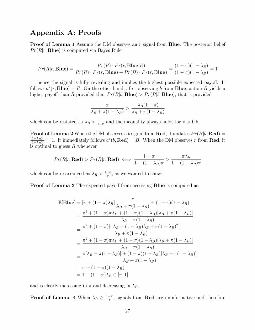
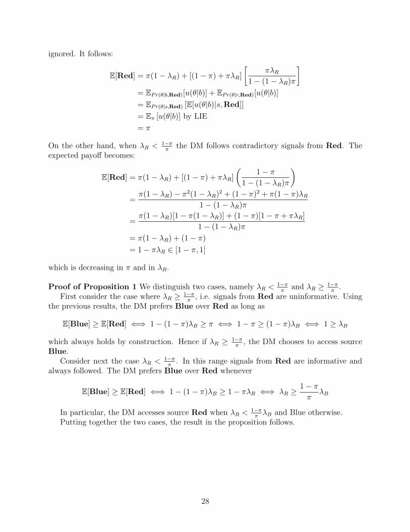
Appendix A: Proofs

Proof of Lemma 1 Assume the DM observes an r signal from Blue. The posterior beliefPr(R|r,Blue) is computed via Bayes Rule:

Pr(R|r,Blue) =Pr(R) · Pr(r,Blue|R)

Pr(R) · Pr(r,Blue) + Pr(B) · Pr(r,Blue)=

(1− π)(1− λB)

(1− π)(1− λB)= 1

hence the signal is fully revealing and implies the highest possible expected payoff. Itfollows a∗(r,Blue) = R. On the other hand, after observing b from Blue, action B yields ahigher payoff than R provided that Pr(B|b,Blue) > Pr(R|b,Blue), that is provided

π

λB + π(1− λB)>

λB(1− π)

λB + π(1− λB)

which can be restated as λB <π

1−π and the inequality always holds for π > 0.5.

Proof of Lemma 2 When the DM observes a b signal from Red, it updates Pr(B|b,Red) =(1−λR)π(1−λR)π

= 1. It immediately follows a∗(b,Red) = B. When the DM observes r from Red, itis optimal to guess R whenever

Pr(R|r,Red) > Pr(B|r,Red) ⇐⇒ 1− π1− (1− λR)π

>πλR

1− (1− λR)π

which can be re-arranged as λR <1−ππ

, as we wanted to show.

Proof of Lemma 3 The expected payoff from accessing Blue is computed as:

E[Blue] = [π + (1− π)λB]π

λB + π(1− λB)+ (1− π)(1− λB)

=π2 + (1− π)πλB + (1− π)(1− λB)[λB + π(1− λB)]

λB + π(1− λB)

=π2 + (1− π)[πλB + (1− λB)λB + π(1− λB)2]

λB + π(1− λB)

=π2 + (1− π)πλB + (1− π)(1− λB)[λB + π(1− λB)]

λB + π(1− λB)

=π[λB + π(1− λB)] + (1− π)(1− λB)[λB + π(1− λB)]

λB + π(1− λB)

= π + (1− π)(1− λB)

= 1− (1− π)λB ∈ [π, 1]

and is clearly increasing in π and decreasing in λB.

Proof of Lemma 4 When λR ≥ 1−ππ

, signals from Red are uninformative and therefore

27

ignored. It follows:

E[Red] = π(1− λR) + [(1− π) + πλR]

[πλR

1− (1− λR)π

]= EPr(θ|b,Red)[u(θ|b)] + EPr(θ|r,Red)[u(θ|b)]= EPr(θ|s,Red) [E[u(θ|b)|s,Red]]

= Eπ [u(θ|b)] by LIE

= π

On the other hand, when λR < 1−ππ

the DM follows contradictory signals from Red. Theexpected payoff becomes:

E[Red] = π(1− λR) + [(1− π) + πλR]

(1− π

1− (1− λR)π

)=π(1− λR)− π2(1− λR)2 + (1− π)2 + π(1− π)λR

1− (1− λR)π

=π(1− λR)[1− π(1− λR)] + (1− π)[1− π + πλR]

1− (1− λR)π

= π(1− λR) + (1− π)

= 1− πλR ∈ [1− π, 1]

which is decreasing in π and in λR.

Proof of Proposition 1 We distinguish two cases, namely λR <1−ππ

and λR ≥ 1−ππ

.First consider the case where λR ≥ 1−π

π, i.e. signals from Red are uninformative. Using

the previous results, the DM prefers Blue over Red as long as

E[Blue] ≥ E[Red] ⇐⇒ 1− (1− π)λB ≥ π ⇐⇒ 1− π ≥ (1− π)λB ⇐⇒ 1 ≥ λB

which always holds by construction. Hence if λR ≥ 1−ππ

, the DM chooses to access sourceBlue.

Consider next the case λR < 1−ππ

. In this range signals from Red are informative andalways followed. The DM prefers Blue over Red whenever

E[Blue] ≥ E[Red] ⇐⇒ 1− (1− π)λB ≥ 1− πλR ⇐⇒ λR ≥1− ππ

λB

In particular, the DM accesses source Red when λR <1−ππλB and Blue otherwise.

Putting together the two cases, the result in the proposition follows.

28

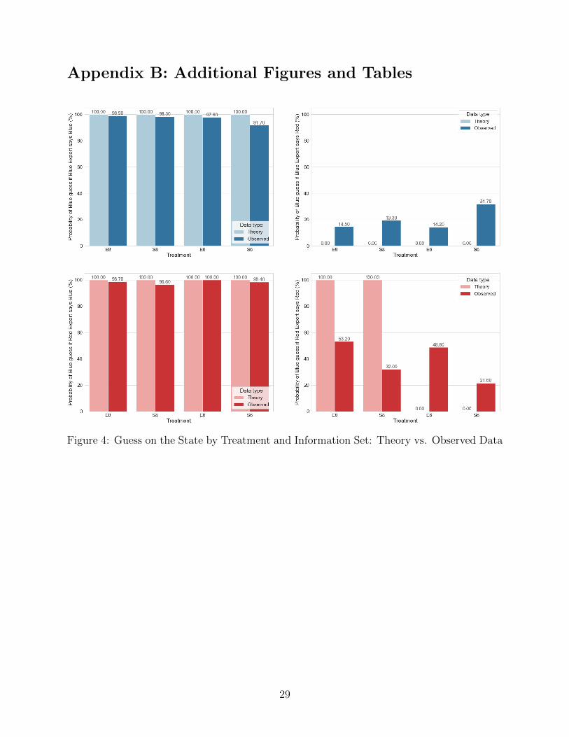
Appendix B: Additional Figures and Tables

Figure 4: Guess on the State by Treatment and Information Set: Theory vs. Observed Data

29

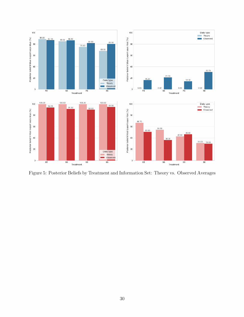
Figure 5: Posterior Beliefs by Treatment and Information Set: Theory vs. Observed Averages

30

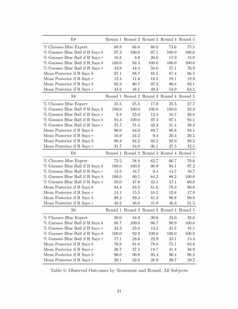
E8 Round 1 Round 2 Round 3 Round 4 Round 5

% Chooses Blue Expert 69.8 66.0 66.0 73.6 75.5% Guesses Blue Ball if B Says b 97.3 100.0 97.1 100.0 100.0% Guesses Blue Ball if B Says r 10.8 8.6 20.0 17.9 15.0% Guesses Blue Ball if R Says b 100.0 94.4 100.0 100.0 100.0% Guesses Blue Ball if R Says r 43.8 44.4 50.0 57.1 76.9Mean Posterior if B Says b 87.1 88.7 85.5 87.4 86.5Mean Posterior if B Says r 12.4 11.6 18.5 19.1 18.9Mean Posterior if R Says b 92.3 90.7 97.2 96.8 93.1Mean Posterior if R Says r 43.2 48.1 49.3 53.9 63.5

S8 Round 1 Round 2 Round 3 Round 4 Round 5


E6 Round 1 Round 2 Round 3 Round 4 Round 5


S6 Round 1 Round 2 Round 3 Round 4 Round 5


Table 5: Observed Outcomes by Treatment and Round, All Subjects

31

E81+ Correct Answers

(N = 265)2+ Correct Answers

(N = 245)3 Correct Answers

(N = 145)

% Chooses Blue Expert 70.7 70.2 73.8% Guesses Blue Ball if B Says b 97.0 98.8 100.0% Guesses Blue Ball if B Says r 0.0 15.1 11.2% Guesses Blue Ball if R Says b 95.1 98.6 97.4% Guesses Blue Ball if R Says r 48.8 54.8 65.8Mean Posterior if B Says b 82.6 87.1 87.0Mean Posterior if B Says r 0.9 14.6 12.6Mean Posterior if R Says b 94.5 95.1 93.2Mean Posterior if R Says r 49.0 51.7 60.9

S81+ Correct Answers



(N = 75)


E61+ Correct Answers



(N = 140)


S61+ Correct Answers



(N = 110)


Table 6: Observed Outcomes by Performance in Comprehension Quiz, All Rounds

32

Equal Reliability, Prior = 0.8 (E8) N Observed Theory

Mean Posterior if B Says b 186 87.1 88.9Mean Posterior if B Says r 186 16.2 0Mean Posterior if R Says b 79 94.0 100Mean Posterior if R Says r 79 50.9 66.7

Skewed Reliability, Prior = 0.8 (S8) N Observed Theory


Equal Reliability, Prior = 0.6 (E6) N Observed Theory


Skewed Reliability, Prior = 0.6 (S6) N Observed Theory


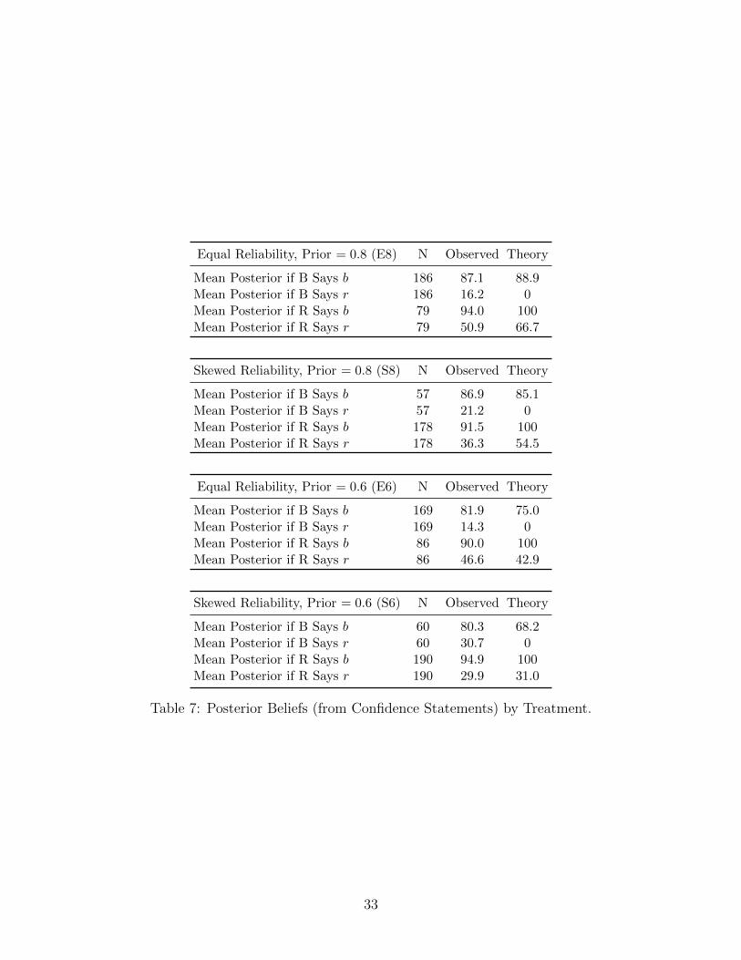
Table 7: Posterior Beliefs (from Confidence Statements) by Treatment.

33

Appendix C: Sample Instructions (Treatment E8)

Experimental instructions were delivered in the initial screens of the experiment. We reporthere the complete text and figures of these screens, including the comprehension quiz andthe practice round. Page titles, as they appeared on the participants’ screen, are in bold.

WELCOMEWelcome!Thank you for agreeing to participate in this experiment!This is an experiment designed to study how people make decisions.The whole experiment will last around 10 minutes.In addition to your participation fee, you will be able to earn a bonus payment.Your bonus payment will depend on your choices so, please, read the instructions carefully.We will use only one decision to determine your bonus payment but all decisions are equallylikely to be selected so all choices matter. The instructions describe how your choices affectsyour earnings. They are composed of three pages and include a comprehension question atthe end of each page.Please, devote at least 5 minutes to the instructions and the comprehension questions.Once you start the experiment, we require your complete and undistracted attention.When you are ready to start, please click the button below:

NEXT

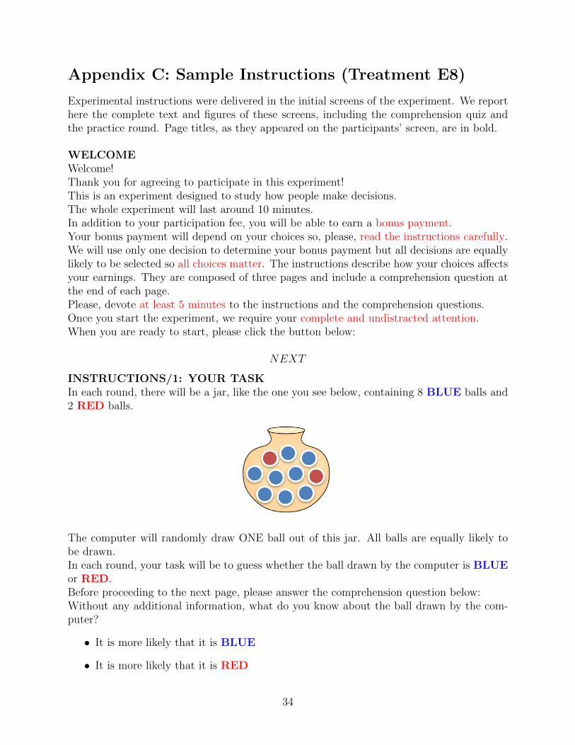
INSTRUCTIONS/1: YOUR TASKIn each round, there will be a jar, like the one you see below, containing 8 BLUE balls and2 RED balls.

The computer will randomly draw ONE ball out of this jar. All balls are equally likely tobe drawn.In each round, your task will be to guess whether the ball drawn by the computer is BLUEor RED.Before proceeding to the next page, please answer the comprehension question below:Without any additional information, what do you know about the ball drawn by the com-puter?

• It is more likely that it is BLUE

• It is more likely that it is RED

34

• It is just as likely that it is BLUE as that it is RED

Please spend at least 30 seconds on this page. Read the instructions carefully! :-)

NEXT

FEEDBACK/1Correct!The urn contains 10 balls in total: 8 BLUE balls and 2 RED balls.The computer draws one ball completely at random: each of the 10 balls is equally likely tobe drawn.This means that there are 8 chances out of 10 that the computer draws a BLUE ball and2 chances out of 10 that the computer draws a RED ball.Thus, without any additional information, you know that the ball is more likely to be BLUE.

NEXT

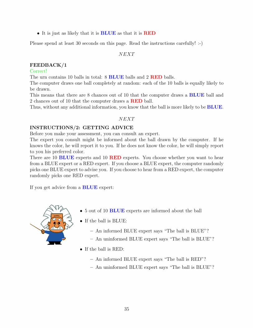
INSTRUCTIONS/2: GETTING ADVICEBefore you make your assessment, you can consult an expert.The expert you consult might be informed about the ball drawn by the computer. If heknows the color, he will report it to you. If he does not know the color, he will simply reportto you his preferred color.There are 10 BLUE experts and 10 RED experts. You choose whether you want to hearfrom a BLUE expert or a RED expert. If you choose a BLUE expert, the computer randomlypicks one BLUE expert to advise you. If you choose to hear from a RED expert, the computerrandomly picks one RED expert.

If you get advice from a BLUE expert:

• 5 out of 10 BLUE experts are informed about the ball

• If the ball is BLUE:

– An informed BLUE expert says “The ball is BLUE”?

– An uninformed BLUE expert says “The ball is BLUE”?

• If the ball is RED:

– An informed BLUE expert says “The ball is RED”?


35

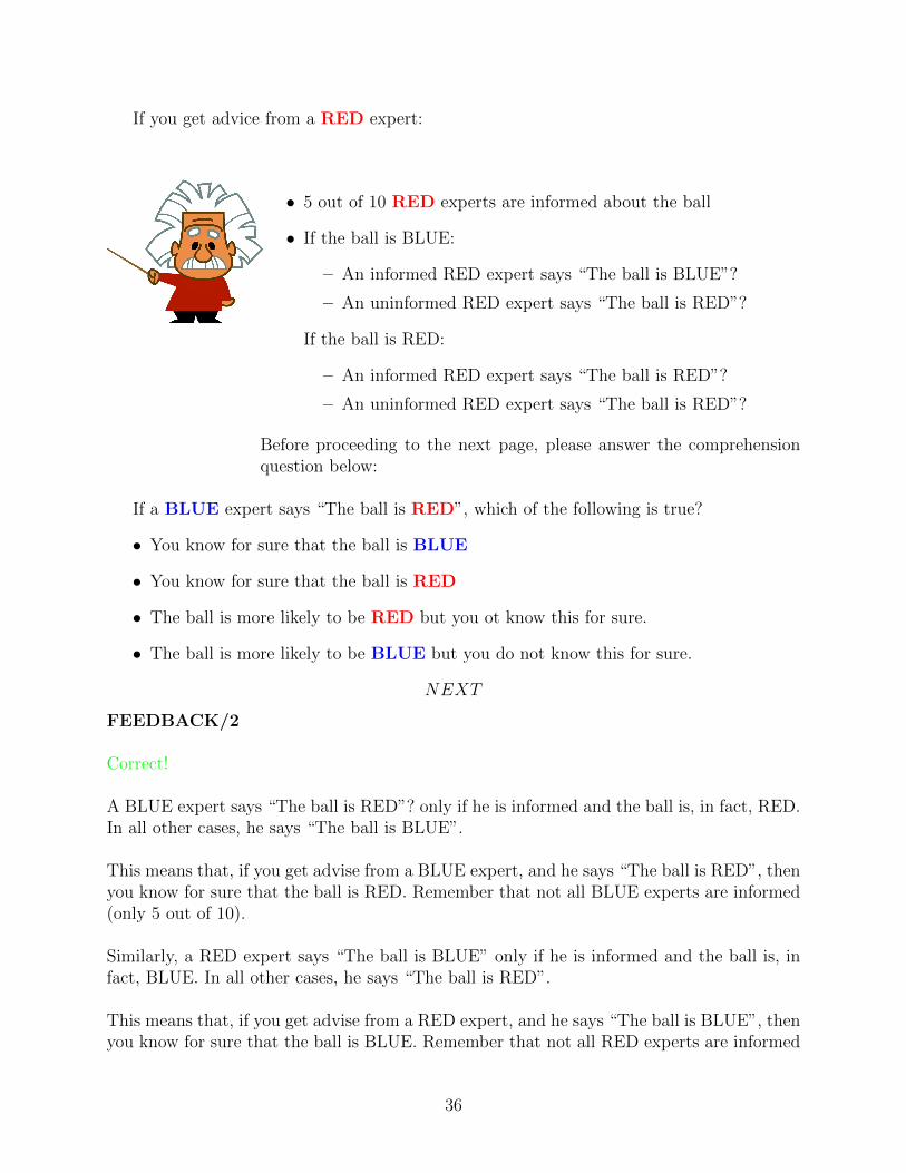
If you get advice from a RED expert:

• 5 out of 10 RED experts are informed about the ball


– An informed RED expert says “The ball is BLUE”?

– An uninformed RED expert says “The ball is RED”?

If the ball is RED:

– An informed RED expert says “The ball is RED”?


Before proceeding to the next page, please answer the comprehensionquestion below:

If a BLUE expert says “The ball is RED”, which of the following is true?

• You know for sure that the ball is BLUE

• You know for sure that the ball is RED

• The ball is more likely to be RED but you ot know this for sure.

• The ball is more likely to be BLUE but you do not know this for sure.

NEXT

FEEDBACK/2

Correct!

A BLUE expert says “The ball is RED”? only if he is informed and the ball is, in fact, RED.In all other cases, he says “The ball is BLUE”.

This means that, if you get advise from a BLUE expert, and he says “The ball is RED”, thenyou know for sure that the ball is RED. Remember that not all BLUE experts are informed(only 5 out of 10).

Similarly, a RED expert says “The ball is BLUE” only if he is informed and the ball is, infact, BLUE. In all other cases, he says “The ball is RED”.

This means that, if you get advise from a RED expert, and he says “The ball is BLUE”, thenyou know for sure that the ball is BLUE. Remember that not all RED experts are informed

36

(only 5 out of 10).

NEXT

INSTRUCTIONS / 3: GUESS THE COLOR AND EARN MONEY!

After you choose what expert to consult, but before you are revealed his message, you willbe asked to make your best guess about the color of the ball, depending on what you willhear from the expert.Since you can receive two different messages, you will be asked two questions:

What is your guess about the color of the ball, if the expert says “The ball is BLUE”?What is your guess about the color of the ball, if the expert says “The ball is RED”?

After you submit your answers, the computer will report you the expert’s message and willuse as your guess for this round the answer to the corresponding question. For example,if the expert you consulted says “The ball is BLUE”, the computer will use as your guessthe answer you gave to the first question above. If, instead, the expert says ”The ball isRED”, the computer will use as your guess the answer you gave to the second question above.

Your guess will determine your bonus payment in the following way:

You will earn $1 if your guess matches the true color of the ball.You will earn $0 if your guess does not match the true color of the ball.

In addition, you will be asked how confident you are of each of your guesses, on a scalebetween 0 and 100. For example, 0 indicates that you think it is just as likely that you areright or wrong (that is, you think that it is just as likely that the ball is BLUE or RED),while 100 indicates that you are sure you picked the right color (that is, you think you knowfor sure whether the ball is BLUE or RED).

These assessments do not affect your bonus payment but it is very important to us that youmake your choice carefully and that you report to us what you really believe.

Before proceeding to the next page, please answer the comprehension question below:

Consider this example. Your guesses are that the ball is BLUE if the expert says BLUE;and that the ball is RED if the expert says RED. The expert says “The ball is BLUE”? andthe true color of the ball is BLUE. What is your bonus payment in this round?

• $1 because your guess is BLUE and it coincides with the actual color of the ball.

• $0.50 because only one of your two guesses coincides with the actual color of the ball.

• $0 because your guess is RED and it does not coincides with the actual color of theball.

37

Please spend at least 60 seconds on this page. Read the instructions carefully! :-)

NEXT

FEEDBACK/3

Correct!

Only one guess matters for your bonus payment.The guess that matters depends on the message you receive from the expert.Since you do not know what message you will receive, make both guesses carefully.

If the expert says “The ball is BLUE”, the guess that matters for your bonus payment isthe answer to the question: What is your guess about the color of the ball, if the expert says“The ball is BLUE”?If the expert says “The ball is RED”, the guess that matters for your bonus payment is theanswer to the question: What is your guess about the color of the ball, if the expert says“The ball is RED”?

In this example, the expert said BLUE; your guess, conditional on the expert saying BLUE,was BLUE and, thus, your guess for this round was: BLUE.The ball randomly drawn by the computer was BLUE too. This means that your guesscoincided with the ball drawn by the computer and, thus, you earned $1. You earn $0 ifyour guess does not match the color of the ball.

NEXT

GET READY FOR THE GAME!

You will play 5 rounds of this game.The computer will randomly pick one round to determine your bonus payment but all roundsare equally likely to be selected so all choices matter.In each round, there are a new jar with 10 balls, 10 new BLUE Experts, and 10 new REDExperts. The chance the computer draws a RED ball or a BLUE ball from the jar, as wellas the chance that the expert you consult is informed or uninformed are not affected in anyway by what happened in the previous rounds.

When you are ready to start with Round 1, please click the button below.Please spend at least 30 seconds on this page. Read the instructions carefully! :-)

NEXT

PRACTICE ROUND - WHOSE ADVICE DO YOU WANT?

38

There is a jar containing 8 BLUE balls and 2 RED balls.The computer has randomly drawn ONE ball out of this jar.

Your task is to guess whether the ball drawn by the computer is BLUE or RED.

Before you make your guess, you can get advice from a BLUE or a RED expert.If you get advice from a BLUE expert:


– An informed BLUE expert says “The ball is BLUE”?


• If the ball is RED:

– An informed BLUE expert says “The ball is RED”?


If you get advice from a RED expert:


– An informed RED expert says “The ball is BLUE”?


If the ball is RED:

– An informed RED expert says “The ball is RED”?


Remember that 5 out of 10 BLUE experts are informed and 5 out of 10 RED experts areinformed.

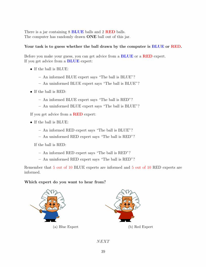
Which expert do you want to hear from?

(a) Blue Expert (b) Red Expert

NEXT

39

PRACTICE ROUND - GUESS THE COLOR!

You decided to consult a BLUE Expert.What is your guess about the color of the ball, if the expert says “The ball is BLUE”?

BLUE

RED

On a scale from 0 to 100, how confident are you about this guess? For example, 0 meansthat you think it is just as likely that you are right or wrong and 100 means you are sureyour guess is correct.

CONFIDENCE

What is your guess about the color of the ball, if the expert says “The ball is RED”?

BLUE

RED

On a scale from 0 to 100, how confident are you about this guess? For example, 0 meansthat you think it is just as likely that you are right or wrong and 100 means you are sureyour guess is correct.

CONFIDENCE

NEXT

PRACTICE ROUND - RESULTS

You decided to consult a BLUE Expert.This expert reported “The ball is BLUE”.Your guess, given the expert’s report, was: BLUE.The ball randomly drawn by the computer in this round was BLUE.Your earnings in this round are $1.00.When you are ready to start with the next round, please click the button below.

NEXT

40

Date post:	19-Feb-2020
Category:	Documents
Upload:	others
View:	14 times
Download:	0 times

Audi Alteram Partem: An Experiment on Selective …salvatorenunnari.eu/mn_selectexposure.pdfAudi...

Documents