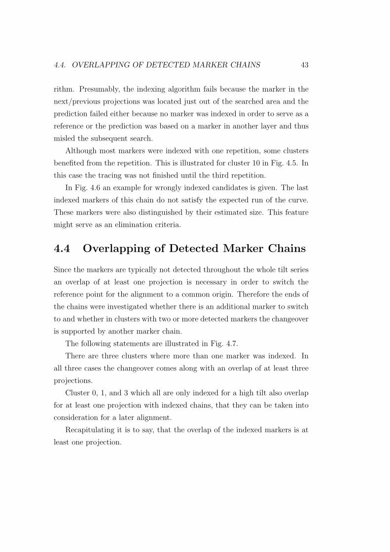
Fachhochschule Hamburg Fachbereich Naturwissenschaftliche Technik Alignment of Transmission Electron Microscopy Images Acquired During a Tilt Series by Tracking Fiducial Markers Diplomarbeit im Studiengang Medizintechnik vorgelegt von Kerstin Stockmeier aus Ludwigshafen am Rhein 10. November 2000 Gutachter: Prof. Dr. Manfred Herbst, FH Hamburg Dr. Thomas K¨ ohler, Philips GmbH Forschungslaboratorien, Hamburg
Transcript
Fachhochschule HamburgFachbereich
Naturwissenschaftliche Technik
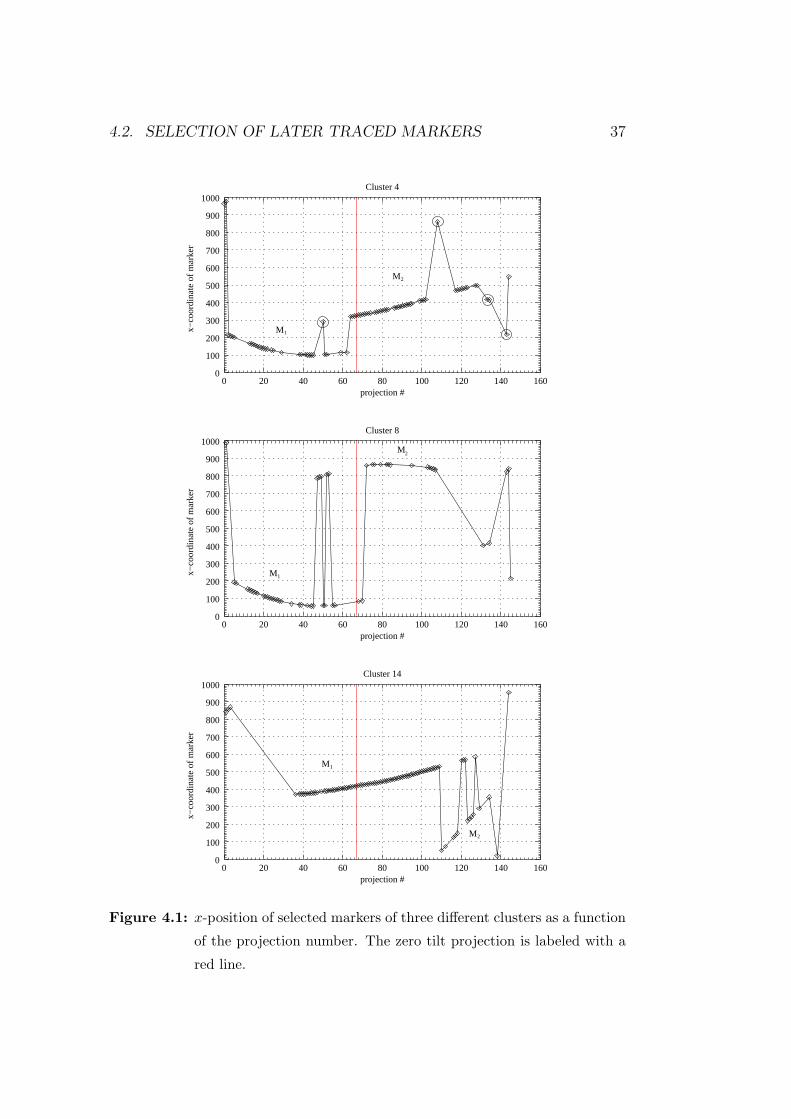
Alignment of
Transmission Electron Microscopy Images
Acquired During a Tilt Series
by Tracking Fiducial Markers
Diplomarbeit
im Studiengang Medizintechnik
vorgelegt von
Kerstin Stockmeier
aus
Ludwigshafen am Rhein
10. November 2000
Gutachter:
Prof. Dr. Manfred Herbst, FH Hamburg
Dr. Thomas Kohler, Philips GmbH Forschungslaboratorien, Hamburg
With electron tomography the 3D structure of an object can be obtained by
reconstructing from a tilt series of 2D projection. This method has been ben-
eficial in biologic research as a high volumetric resolution can be achieved.
It is used for the characterization of macromolecules, viruses, and cellular
organelles in in-vitro preparations [HA96][MBF+95][Rad88][ZPJ+94].
One of the limiting factors of the image quality obtained by the reconstruc-
tion is the precision of alignment of the projections [FM92]. There are dif-
ferent approaches to resolve the alignment step. One approach is to deposit
fiducial markers during the specimen preparation to get easy identifiable
high-contrast regions. At the present time, the acquisition of these mark-
ers often involves operator interaction. This process results in appropriate
accuracy but is tedious and time-consuming should numerous tilt images
come into register. In addition, operator based identification of markers is
a subjective process and requires extensive experience to get a satisfactory
result [RHS+99]. An automatic alignment is commonly done with cross-
correlation [FM92]. But this does not always result in a satisfactory accu-
racy.
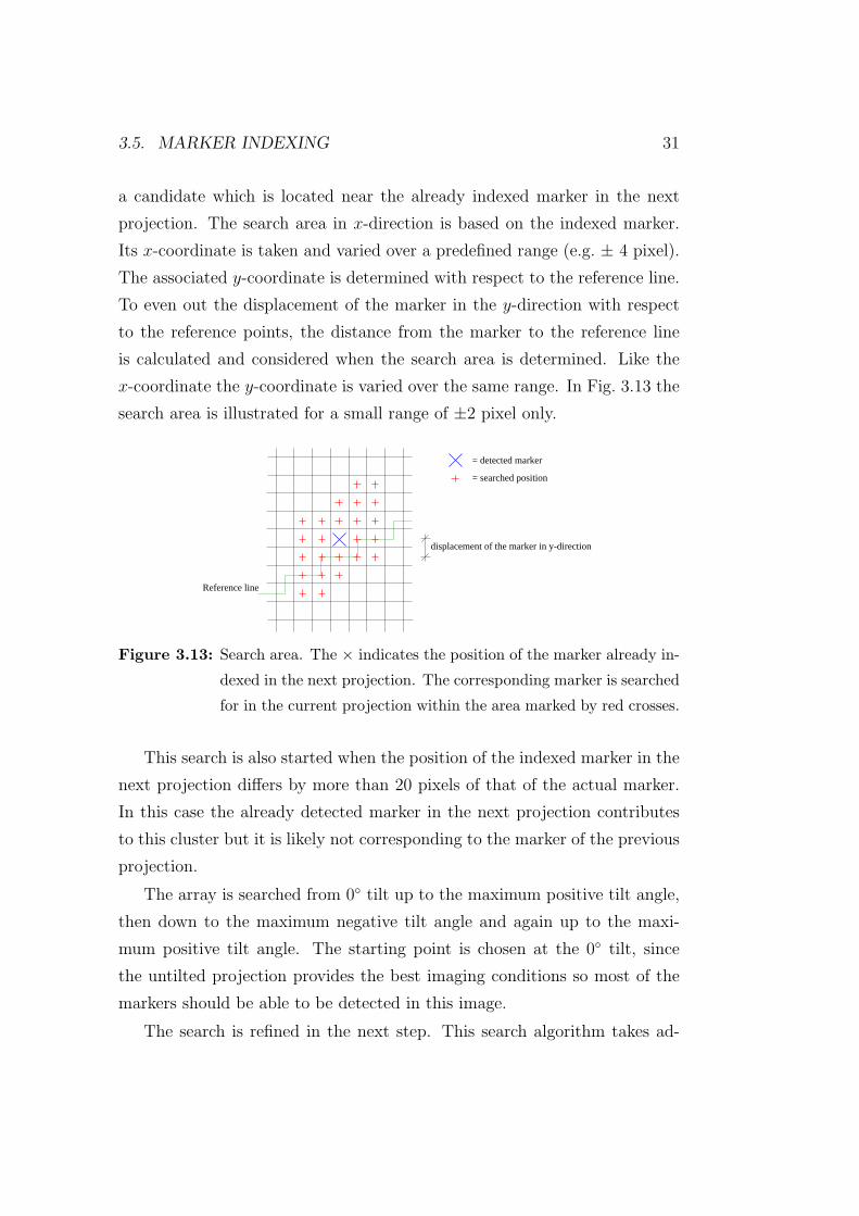
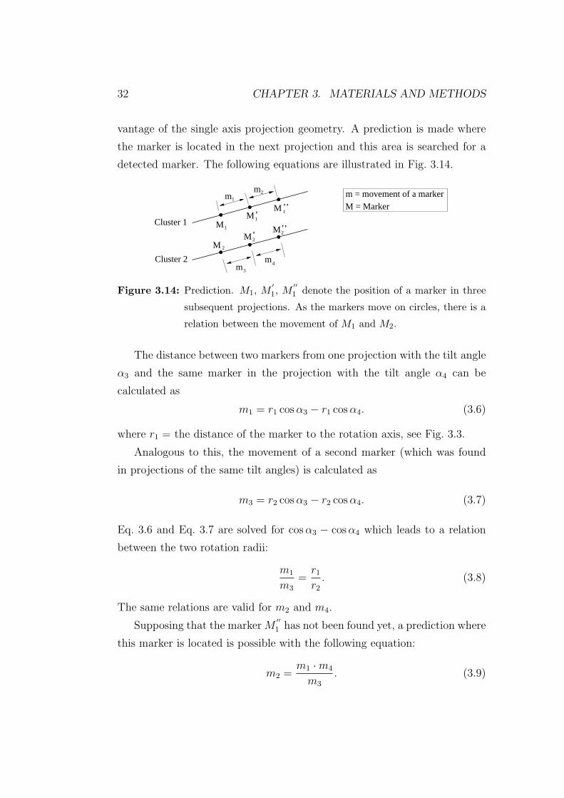
In the following thesis, an alignment method combining cross-correlation with
the tracking of fiducial markers is described in detail. It can be broken down
into three steps: Preprocessing the images with cross-correlation, detection
1
2 CHAPTER 1. INTRODUCTION
of fiducial markers with a pattern recognition algorithm, and establishment
of overlapping chains of indexed markers throughout the tilt series.
This thesis is structured as follows: In chapter two some background infor-
mation is given on the principles of transmission electron microscopy, basic
ideas of 3D electron microscopy and on state of the art aligning 2D projec-
tions using fiducial markers. Chapter three consists of a description of the
image data used and a specification of the registration algorithm. Chap-
ter four summarizes the results obtained with simulated data and real data,
and includes a description of the traceability of the fiducial markers. Chap-
ter five consists of a discussion and concludes with a brief summary of the
perspectives for this method.
Chapter 2
Theoretical Background
2.1 Transmission Electron Microscopy
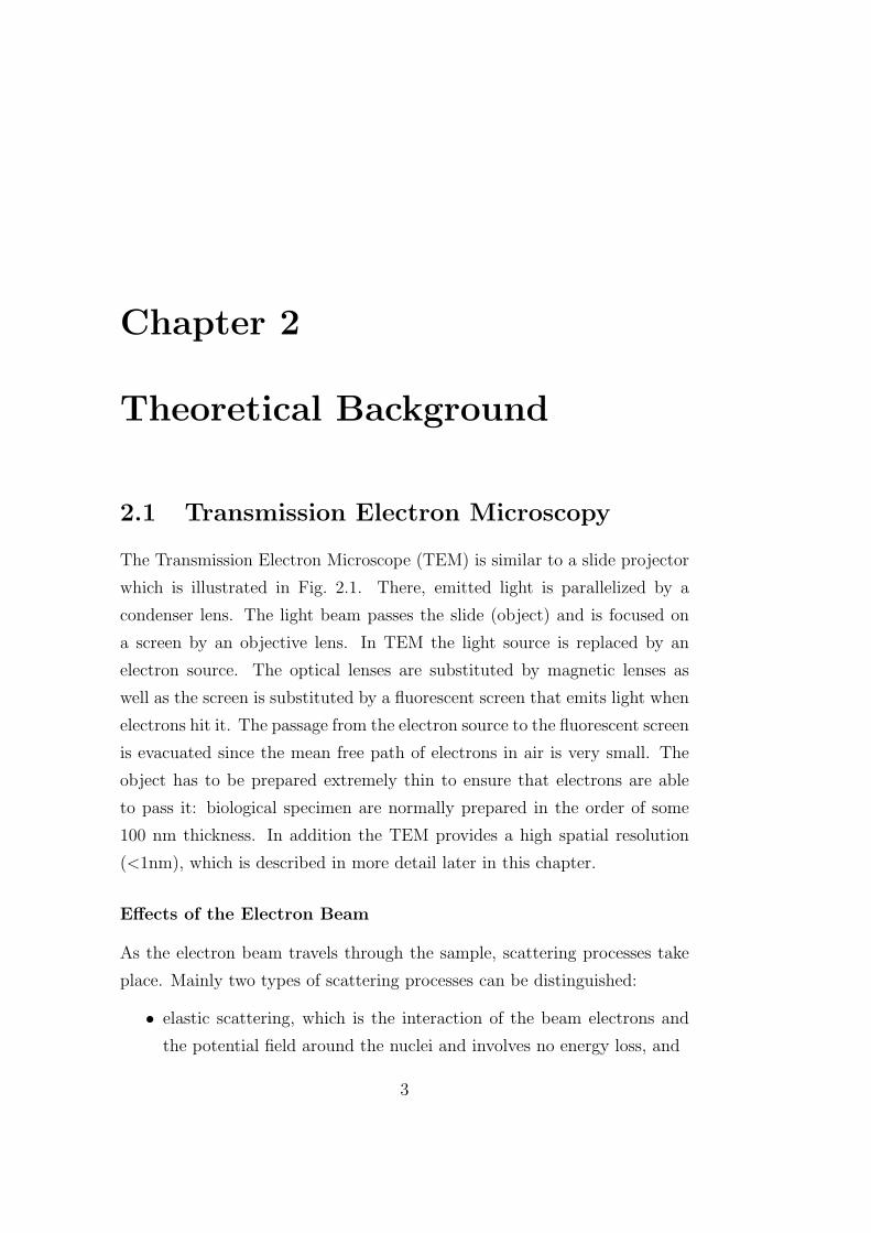
The Transmission Electron Microscope (TEM) is similar to a slide projector
which is illustrated in Fig. 2.1. There, emitted light is parallelized by a
condenser lens. The light beam passes the slide (object) and is focused on
a screen by an objective lens. In TEM the light source is replaced by an
electron source. The optical lenses are substituted by magnetic lenses as
well as the screen is substituted by a fluorescent screen that emits light when
electrons hit it. The passage from the electron source to the fluorescent screen
is evacuated since the mean free path of electrons in air is very small. The
object has to be prepared extremely thin to ensure that electrons are able
to pass it: biological specimen are normally prepared in the order of some
100 nm thickness. In addition the TEM provides a high spatial resolution
(<1nm), which is described in more detail later in this chapter.
Effects of the Electron Beam
As the electron beam travels through the sample, scattering processes take
place. Mainly two types of scattering processes can be distinguished:
• elastic scattering, which is the interaction of the beam electrons and
the potential field around the nuclei and involves no energy loss, and
3
4 CHAPTER 2. THEORETICAL BACKGROUND
Screen
Objective Condenser
Electron source
ApertureFluorescent screen
SlideObjective Condenser
Light source
Electron beam
TEM
Slide projector
Specimen
Figure 2.1: The TEM in comparison with a slide projector. [phi]
• inelastic scattering, which is the interaction of the beam electrons with
the electrons of the sample and involves energy losses and absorption.
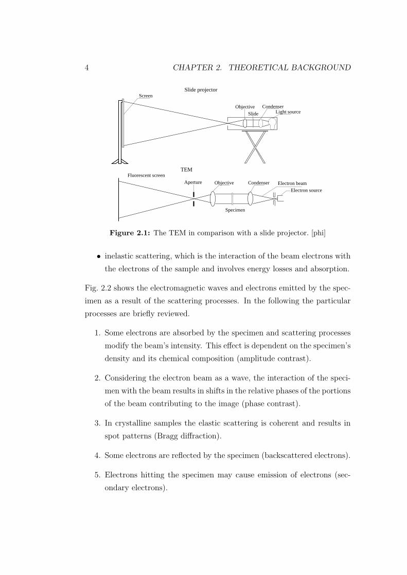
Fig. 2.2 shows the electromagnetic waves and electrons emitted by the spec-
imen as a result of the scattering processes. In the following the particular
processes are briefly reviewed.
1. Some electrons are absorbed by the specimen and scattering processes
modify the beam’s intensity. This effect is dependent on the specimen’s
density and its chemical composition (amplitude contrast).
2. Considering the electron beam as a wave, the interaction of the speci-
men with the beam results in shifts in the relative phases of the portions
of the beam contributing to the image (phase contrast).
3. In crystalline samples the elastic scattering is coherent and results in
spot patterns (Bragg diffraction).
4. Some electrons are reflected by the specimen (backscattered electrons).
5. Electrons hitting the specimen may cause emission of electrons (sec-
ondary electrons).
2.1. TRANSMISSION ELECTRON MICROSCOPY 5
2 θ
Auger electrons
Incidentbeam
Transmitted electrons
Energy loss electrons
Bragg diffracted electrons
Absorbed electrons Specimen
X-Rays
Secondary electrons (low energy)
Backscattered electrons
Cathodoluminescence
Figure 2.2: Interactions of the electron beam with the specimen. [TG79]
6. Electrons hitting the sample may cause it to emit X-rays, whose energy
and wavelength is dependent on the elementary composition of the
sample.
7. Electrons hitting the specimen may cause the sample to emit photons
(light). This process is called cathodoluminescence.
8. Auger Electrons are the final electrons in the Auger emission process.
The primary beam removes an electron from a core level of a sample
atom and leaves a vacancy. Another electron falls from a higher level
into the vacancy thereby releasing energy. This energy is carried of
with the Auger Electron which is ejected from a higher energy level.
In a TEM the first two effects contribute to the image formation of a biological
specimen.
6 CHAPTER 2. THEORETICAL BACKGROUND
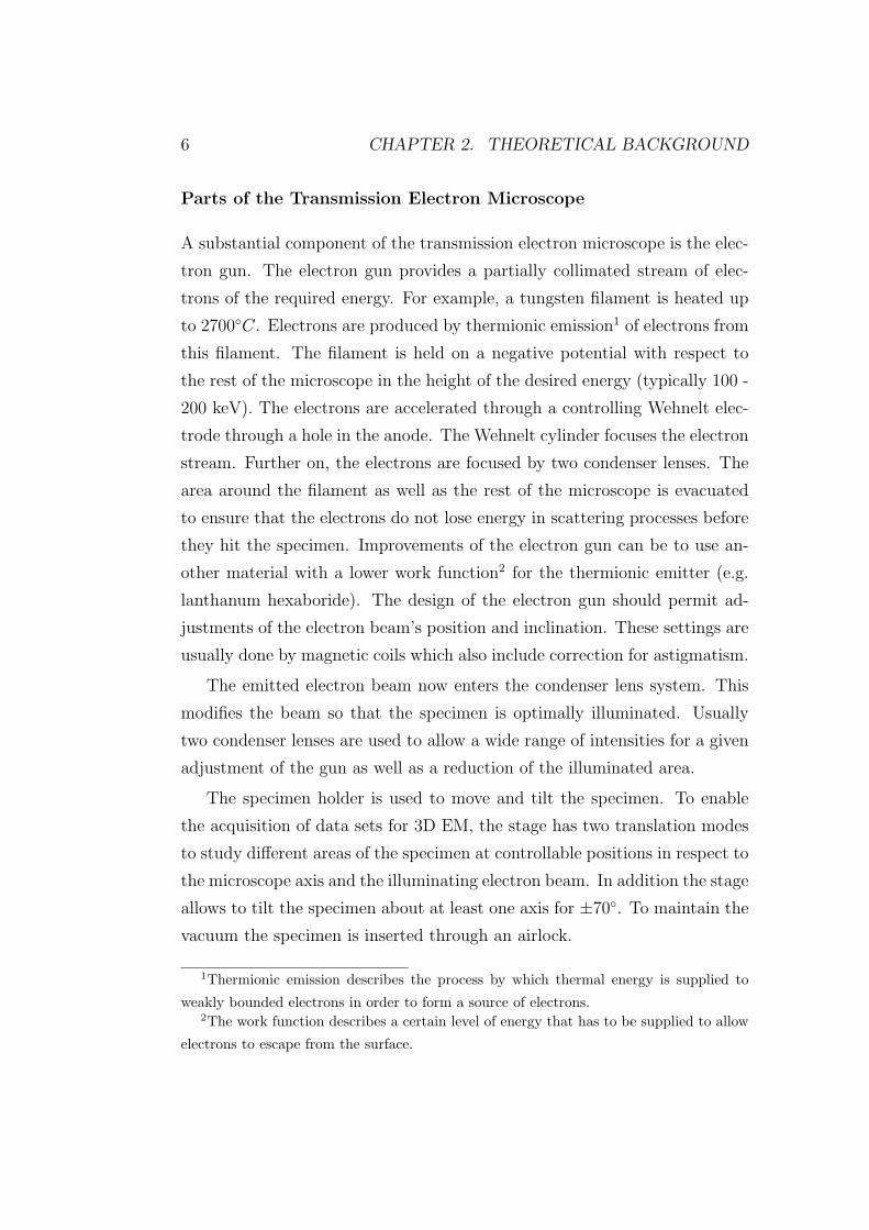
Parts of the Transmission Electron Microscope
A substantial component of the transmission electron microscope is the elec-
tron gun. The electron gun provides a partially collimated stream of elec-
trons of the required energy. For example, a tungsten filament is heated up
to 2700◦C. Electrons are produced by thermionic emission1 of electrons from
this filament. The filament is held on a negative potential with respect to
the rest of the microscope in the height of the desired energy (typically 100 -
200 keV). The electrons are accelerated through a controlling Wehnelt elec-
trode through a hole in the anode. The Wehnelt cylinder focuses the electron
stream. Further on, the electrons are focused by two condenser lenses. The
area around the filament as well as the rest of the microscope is evacuated
to ensure that the electrons do not lose energy in scattering processes before
they hit the specimen. Improvements of the electron gun can be to use an-
other material with a lower work function2 for the thermionic emitter (e.g.
lanthanum hexaboride). The design of the electron gun should permit ad-
justments of the electron beam’s position and inclination. These settings are
usually done by magnetic coils which also include correction for astigmatism.
The emitted electron beam now enters the condenser lens system. This
modifies the beam so that the specimen is optimally illuminated. Usually
two condenser lenses are used to allow a wide range of intensities for a given
adjustment of the gun as well as a reduction of the illuminated area.
The specimen holder is used to move and tilt the specimen. To enable
the acquisition of data sets for 3D EM, the stage has two translation modes
to study different areas of the specimen at controllable positions in respect to
the microscope axis and the illuminating electron beam. In addition the stage
allows to tilt the specimen about at least one axis for ±70◦. To maintain the
vacuum the specimen is inserted through an airlock.
1Thermionic emission describes the process by which thermal energy is supplied to
weakly bounded electrons in order to form a source of electrons.2The work function describes a certain level of energy that has to be supplied to allow
electrons to escape from the surface.
2.1. TRANSMISSION ELECTRON MICROSCOPY 7
Figure 2.3: A schematic drawing of a modern TEM. [TG79]
The optical magnification system of a TEM consists of the objective lens
followed by one or more projector lenses. The objective lens determines the
resolution and contrast of the image. The following lenses are used to magnify
the image for observation and recording. As the objective lens determines the
resolving power3 of the instrument and performs the first stage of imaging,
it is the most critical lens. A high resolution objective lens has a short focal
length, usually in the order of 1 - 3 mm. Normally the specimen holder is
located within the objective lens so it can be part of the condenser system.
3The resolving power of an instrument is the resolution which can be attained under
optimal viewing conditions.
8 CHAPTER 2. THEORETICAL BACKGROUND
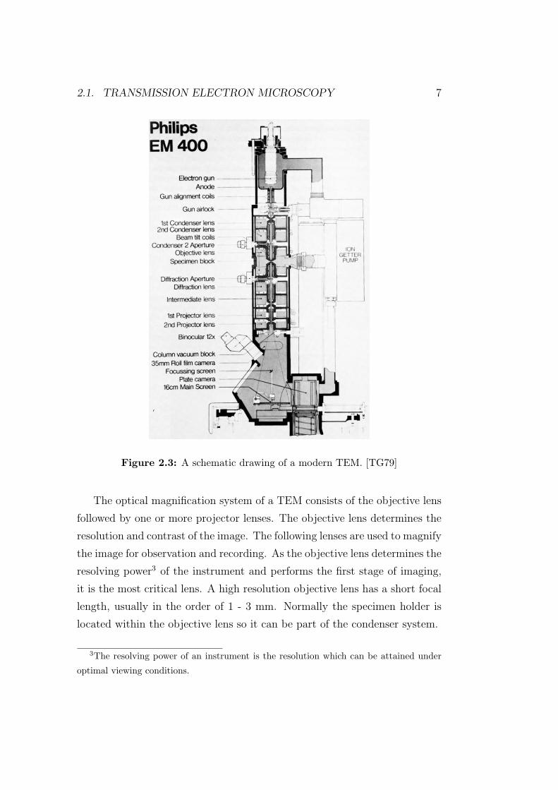
There are sets of apertures in three locations:
• In the condenser system to collimate the electron beam as well as to
modify its intensity;
• In the back focal plane to select electrons at a particular inclination for
a later magnification;
• In the image plane to select electrons from a particular area of interest
or for selected area diffraction.
The lenses are of magnetic type. They are supplied with a highly stabilized
current source which is in addition variable for focusing. The lenses are
designed for a high resolution, i.e. close to atomic level.
There are three major aberrations: spherical aberration (the lens fails to
bring central and peripheral rays into a common focus), chromatic aberration
(the lens fails to bring electrons of a different wavelength into a common
focus) and astigmatism (a circle in the specimen transform to an ellipse in
the image). The spherical aberration is closely related to the design and
the manufacturing of the lens. Chromatic aberrations can be reduced by
stabilizing the accelerating voltage and by using thin specimen, since the
velocity and thus the wavelength of electrons is influenced by fluctuations in
the high tension supply, and by the influence of inelastic scattering with the
specimen. The wavelength of electrons is closely related to their velocity, see
Eq. 2.4. Astigmatism can be corrected by the application of a compensating
magnetic field.
The described parts of the TEM are shown in Fig. 2.1.
Depth of field and focus. In comparison to a light microscope the
depth of field and focus is extremely large. This effect is a result of the small
electron wavelength and the small angular apertures of the imaging lenses.
The depth of field is the distance along the axis on the object side over which
the object can be moved and still resulting in a maximally sharp image. As
2.1. TRANSMISSION ELECTRON MICROSCOPY 9
� � � �� � � �� � � �
� � � �� � � �� � � �
� � � � �� � � � �� � � � �
� � � � �� � � � �� � � � �
Optic axis
Magnetic lens
α
T
Q
B
Back focal plane
A
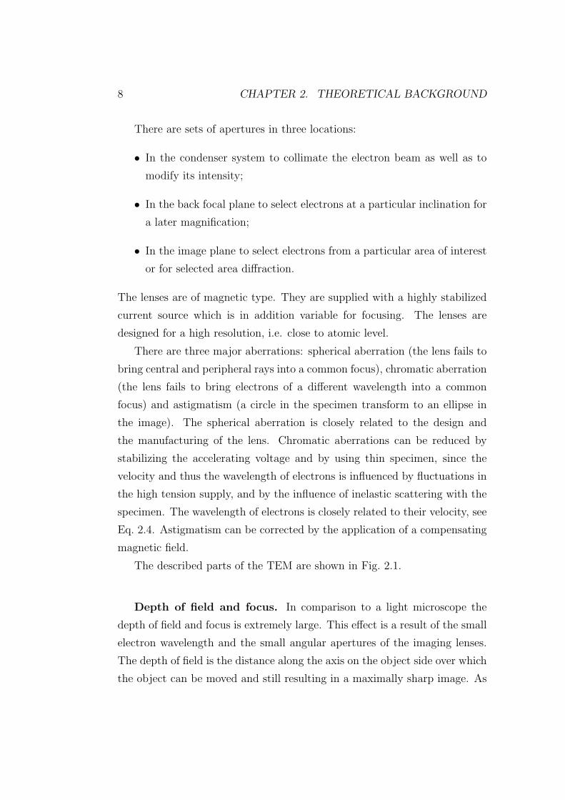
Figure 2.4: Separation of object points P and Q is the resolution limit d. Rays
from these points cross the optical axis at A and B and are equally
sharp. T = A−B is the depth of field. [TG79]
shown in Fig. 2.4 the depth of field T is given as
d
2=
T
2tan α, (2.1)
where α is the lens aperture and d is the resolution, or
T =d
α(since tan α ' α for α � 1). (2.2)
For d = 1nm and α ' 2 · 10−3rad(≈ 1◦),
T = 500nm,
which is much larger than possible with light microscopy because in the latter
α may be 1.22rad (70◦) [TG79]. Hence for an object of ∼ 12µm thickness all
features of the object are focused at once, and a projection of the in focus
three-dimensional object is obtained.
The depth of focus is a finite distance along the optical axis where the
image appears equally sharp. The depth of focus Tf and the depth of field
T are related by the magnification M , as follows [TG79]:
Tf = TM2 =dM2
α. (2.3)
Tf can be considered as infinite for all practical purposes, and so it is not
necessary to refocus when exposing plates or film which are not located at
the viewing screen.
10 CHAPTER 2. THEORETICAL BACKGROUND
Figure 2.5: Plot showing resolution d as a function of accelerating voltage and
spherical aberration coefficient Cs. [TG79]
Resolution. As mentioned before, a feature of the TEM is its high spatial
resolution. The resolution is determined by the spherical aberration coeffi-
cient Cs of the objective lens and the the electron wavelength λ, given by the
de Broglie wave relation:
λ =h
mv. (2.4)
with h = Planck’s constant, m = the electron’s mass, and v = the electron’s
velocity.
When passing through a potential difference V an electron is accelerated
to a velocity of
v =
√2eV
m, (2.5)
with e = charge of the electron.
Substituting Eq. 2.5 in Eq. 2.4, the wavelength of an electron is given by:
λ =h√
2meV. (2.6)
Fig. 2.5 shows the resolution d as a function of accelerating voltage and
spherical aberration coefficient Cs. If the spherical aberration coefficient is
2.2. ELECTRON TOMOGRAPHY 11
maintained constant the resolution can be raised by increasing the accelerat-
ing voltage (through decreasing λ). So at 500kV or higher, atomic resolution
becomes theoretically possible even in close-packed structures. The optimum
voltage is determined by the specimen stability and knock-on damage and
by the voltage stabilization [TG79].
2.2 Electron Tomography
Tomography is a method to reconstruct the interior of an object from its
projections. Literally, the word tomography means visualization of slices.
Nowadays the term electron tomography (ET) is used for any technique that
utilizes the TEM to collect projections of an object and reconstructs the
object and its entirety by using these projections.
To properly understand the possibility to reconstruct objects by using its
projections the underlying ideas are briefly summarized.
A fundamental mathematical theorem, the so called Fourier slice theorem
[Jac96], states that the measurement of a projection is equivalent to a mea-
surement of a single central plane of the object’s three-dimensional Fourier
transform. The Fourier transform is an alternative representation of the ob-
ject and breaks down the object’s density distribution into sine waves. The
following condition must be fulfilled for a complete coverage of the object in
Fourier space:
• The strengths (amplitudes) and phase shifts of all sine waves traveling
in all possible directions and having wavelengths down to d/2 have to
be known, where d is the desired resolution of the three-dimensional
object.
By tilting the object around a single axis through a range of ±90◦, the Fourier
transform is completely sampled. Here, the angular increments have to be
small enough to prevent information loss. The relation between resolution d
12 CHAPTER 2. THEORETICAL BACKGROUND
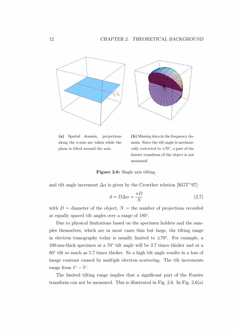
(a) Spatial domain, projections
along the z-axis are taken while the
plane is tilted around the axis.
(b) Missing data in the frequency do-
main: Since the tilt angle is mechani-
cally restricted to ±70◦, a part of the
fourier transform of the object is not
measured.
Figure 2.6: Single axis tilting.
and tilt angle increment ∆α is given by the Crowther relation [KGT+97]:
d = D∆α =πD
N(2.7)
with D = diameter of the object, N = the number of projections recorded
at equally spaced tilt angles over a range of 180◦.
Due to physical limitations based on the specimen holders and the sam-
ples themselves, which are in most cases thin but large, the tilting range
in electron tomography today is usually limited to ±70◦. For example, a
100-nm-thick specimen at a 70◦ tilt angle will be 2.7 times thicker and at a
80◦ tilt so much as 5.7 times thicker. So a high tilt angle results in a loss of
image contrast caused by multiple electron scattering. The tilt increments
range from 1◦ − 5◦.
The limited tilting range implies that a significant part of the Fourier
transform can not be measured. This is illustrated in Fig. 2.6. In Fig. 2.6(a)
2.3. IMAGE REGISTRATION 13
a single axis tilt is illustrated. In Fig. 2.6(b) the missing spatial frequencies
in Fourier space are illustrated. Due to the limited tilt angle a wedge shaped
area is missing[Fra92].
Finally the series of two-dimensional data obtained is processed to obtain
a three-dimensional image. For this, the 2D-images have to be aligned with
respect to each other in order to refer them to a common 3-D coordinate
system describing the object to be computed. Up till now, the alignment is
usually done by cross-correlation [FM92] or manually. The 3D-image is then
computed using a reconstruction algorithm of which several types are avail-
able, e.g. Fourier reconstruction methods, weighted backprojection methods,
or iterative direct space methods. A detailed description of reconstruction
methods used in ET is given in [Fra92].
2.3 Image Registration
A major delimiting factor of resolution in the 3D volume is the accuracy
of alignment of the tilt series. Tomographic approaches need to acquire
an image series over a large angular range (usually ±70◦) with small incre-
ments (usually 1◦ − 5◦). The specimen can not be made perfectly eucentric.
Thus specimen tilting results in both X-Y-translation and changes in focus.
Although recently developed systems for automated acquisition of tilt se-
ries [KGT+97] keep track of image shifts and refocusing steps, an additional
alignment step prior to the 3D-reconstruction is necessary.
Alignment. Alignment is an operation that is meant to register one or
more images that contain a common motif. Due to imperfections in the
tilting stage and the necessity of refocusing during the acquisition, the tilt
series set has to be aligned before the 3D reconstruction. Registration and
alignment are used synonymously.
Fiducial marker. As the word fiducial implies this marker is meant to be
imaged reliably throughout the tilt series. In EM usually gold beads are
used. Due to their high density gold beads are imaged as clearly shaped
14 CHAPTER 2. THEORETICAL BACKGROUND
dark spots. In the following, the markers are also referred to as gold beads
or beads. During the registration, an image processing algorithm identifies
features in the projections that look like beads. These features are called
candidates.
Indexing. In order to align an image series it is necessary to establish a cor-
respondence from one image to another. For this, the previously mentioned
fiducial markers are used. These markers not only need to be detected in
every image but also associated to a detected marker in subsequent projec-
tions. The process of associating a detected marker with its corresponding
marker in the next or previous projection respectively is called indexing.
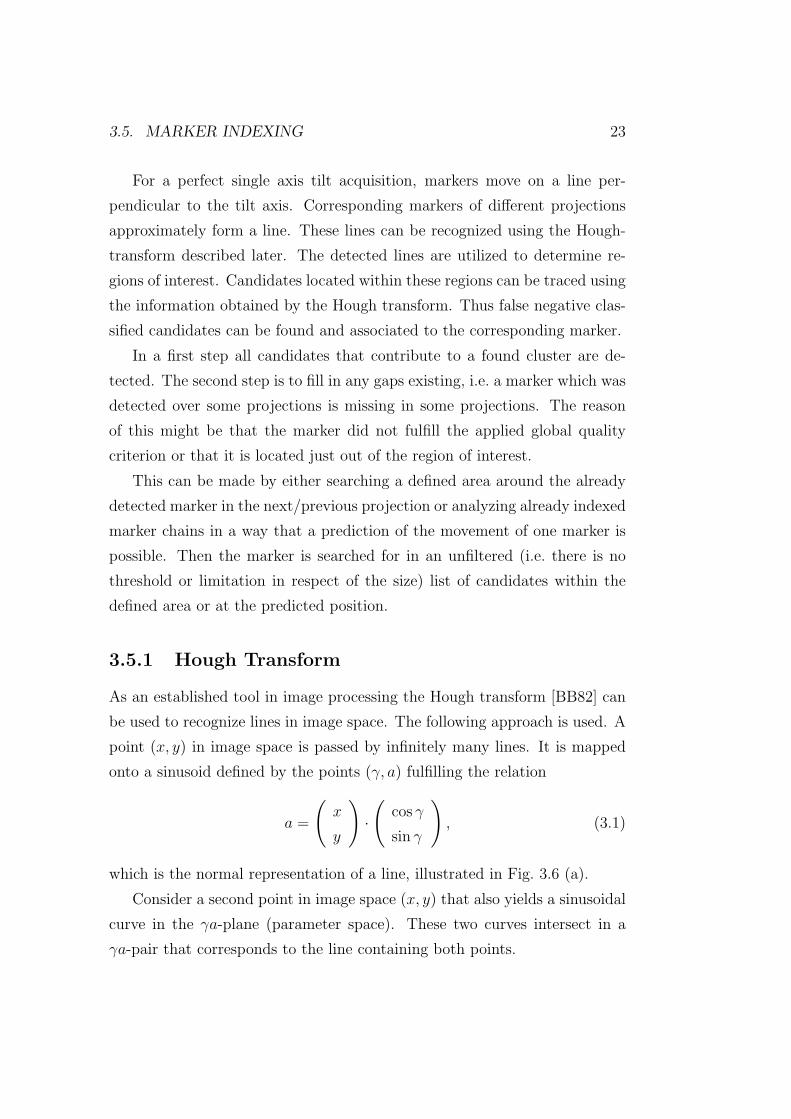
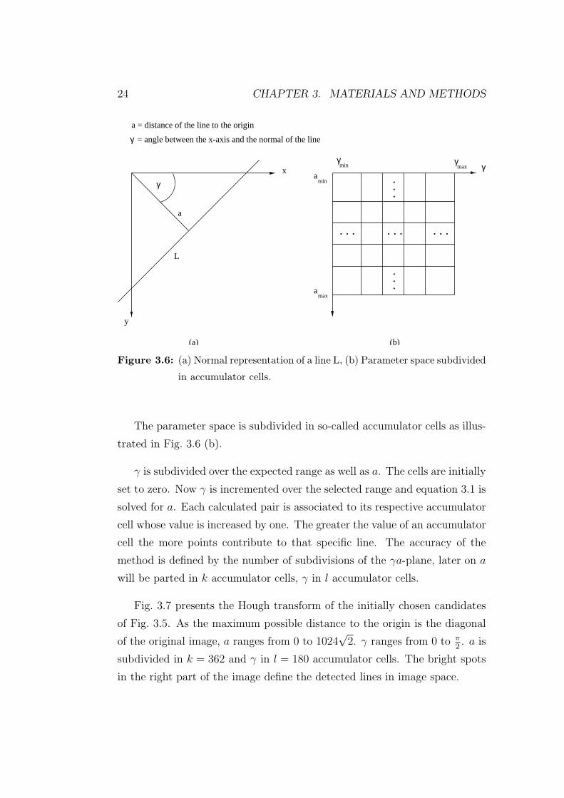
Single-axis tilting of a fiducial marker. For a perfect single-axis tilt
the marker would move on an orbit with radius r around the tilt axis. As
previously described TEM-images are projections along the optical axis. The
orbit projected in a 2D-image results in a line that is perpendicular to the tilt
axis. Line recognition is a well-known procedure in digital image processing
and can be used to recognize regions of interest. The x- and y-coordinates
of the marker as a function of the tilt angle result in a sinusoid according to
the geometric properties of an orbit’s projection.
2.4 Methods for Automatic Alignment of Tilt
Series Using Fiducial Markers
At least two methods of automatic alignment of tilt series using fiducial
markers have been published so far.
Fungh et al. [FLR+96] initially segment out all features throughout the
tilt series that possibly represent beads. Out of the identified gold beads
a set of gold beads in a reference view is interactively determined. These
markers are tracked over the rest of the tilt series. This is done by a simple
prediction of the position of a marker in the next projection. If a candidate
is found near the predicted position, it is taken. If not enough bead positions
2.4. METHODS FOR AUTOMATIC ALIGNMENT 15
were found throughout the entire data stack a more vigorous search is started
which again involves a prediction of the bead position. The method requires
for the prediction a knowledge of the tilt axis which is not known in all cases.
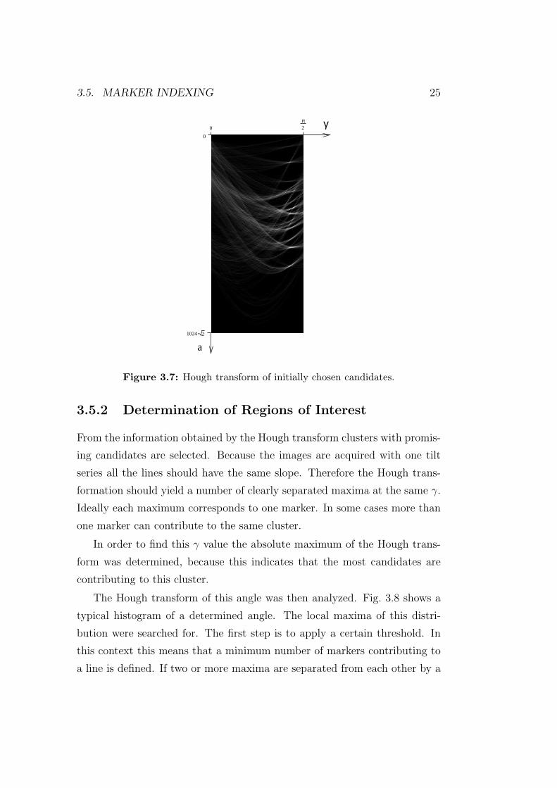
Ress et al. [RHS+99] primarily specify the number of markers to be de-
tected. Here, the threshold for each image is adjusted in a way that the
predefined amount of markers were detected. The binary images containing
the markers are then cross-correlated in order to obtain the relative image
offsets. These offsets are used to compare the markers acquired in the refer-
ence image with those in the unindexed image. If the minimum distance of
an unindexed position falls below a tolerance, the marker is accepted. The
newly accepted markers now serve as the new reference. Compared to Fungh
et al. the selection of candidates to track is more restrictive: Only markers
detected in the zero-tilt reference were tracked.
The approach proposed in this thesis is more flexible concerning the selec-
tion of markers to be tracked. The selection is fully automatic. Furthermore,
the marker must not be represented in a reference view, so it is not necessary
to track a marker over the whole tilt series and it should be feasible to track
markers independently tracked in the begin and end of the series. Besides,
the proposed method does not require a knowledge of the tilt axis like the
procedure of Fung et al. although a prediction is as well included. Thus, this
algorithm should provide more flexibility and a better performance as the
two previously published algorithms.
Chapter 3
Materials and Methods
3.1 Phantom Data
To verify if the rough alignment with the cross-correlation function (CCF) is
working properly, a phantom data set was created using the script language
RADONIS. One data set created represented a perfect single axis tilting
without any shifts. In a second data set the images were shifted with respect
to each other. These shifts were protocolled in a floating point.
3.2 Real Data
The data of a pore in a hyphal cell of rhizoctonia solani1 was obtained by
Bram Koster, University of Utrecht. The Philips CM120 TEM was used. The
images were digitalized with a 10242 charge-coupled device (CCD) camera.
The pixel size is 0.86nm. As manual data collection is very time consuming
an automated data collection routine was used as described in [KGT+97].
The obtained data set included 146 projections. The tilt range goes from
−66◦ up to 79◦ with an increment of 1◦. Though the data set includes
images with a higher tilt angle than 70◦ and these images were taken into
considaration for the later described calculations, but they do not contain
1Rhizoctonia solani is a plant pathogen fungus.
16
3.3. MISALIGNMENT ESTIMATION BY CROSS-CORRELATION 17
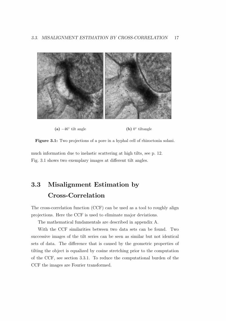
(a) −46◦ tilt angle (b) 0◦ tiltangle
Figure 3.1: Two projections of a pore in a hyphal cell of rhizoctonia solani.
much information due to inelastic scattering at high tilts, see p. 12.
Fig. 3.1 shows two exemplary images at different tilt angles.
3.3 Misalignment Estimation by
Cross-Correlation
The cross-correlation function (CCF) can be used as a tool to roughly align
projections. Here the CCF is used to eliminate major deviations.
The mathematical fundamentals are described in appendix A.
With the CCF similarities between two data sets can be found. Two
successive images of the tilt series can be seen as similar but not identical
sets of data. The difference that is caused by the geometric properties of
tilting the object is equalized by cosine stretching prior to the computation
of the CCF, see section 3.3.1. To reduce the computational burden of the
CCF the images are Fourier transformed.
18 CHAPTER 3. MATERIALS AND METHODS
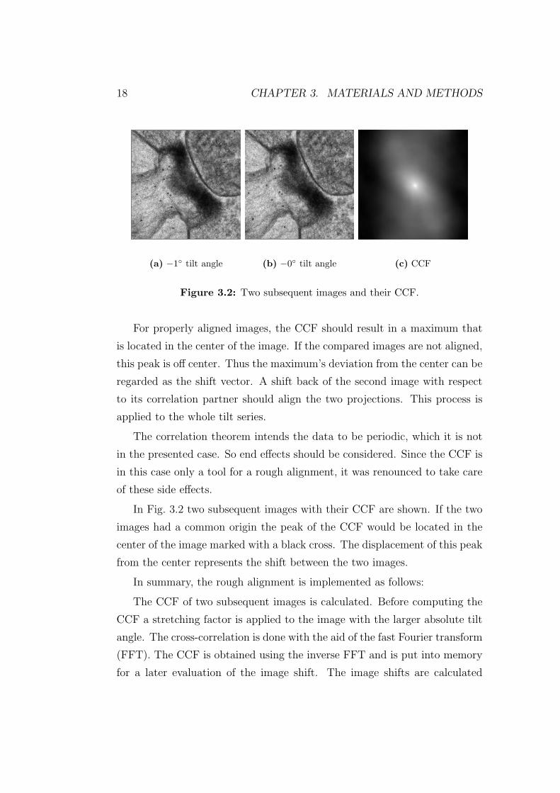
(a) −1◦ tilt angle (b) −0◦ tilt angle (c) CCF
Figure 3.2: Two subsequent images and their CCF.
For properly aligned images, the CCF should result in a maximum that
is located in the center of the image. If the compared images are not aligned,
this peak is off center. Thus the maximum’s deviation from the center can be
regarded as the shift vector. A shift back of the second image with respect
to its correlation partner should align the two projections. This process is
applied to the whole tilt series.
The correlation theorem intends the data to be periodic, which it is not
in the presented case. So end effects should be considered. Since the CCF is
in this case only a tool for a rough alignment, it was renounced to take care
of these side effects.
In Fig. 3.2 two subsequent images with their CCF are shown. If the two
images had a common origin the peak of the CCF would be located in the
center of the image marked with a black cross. The displacement of this peak
from the center represents the shift between the two images.
In summary, the rough alignment is implemented as follows:
The CCF of two subsequent images is calculated. Before computing the
CCF a stretching factor is applied to the image with the larger absolute tilt
angle. The cross-correlation is done with the aid of the fast Fourier transform
(FFT). The CCF is obtained using the inverse FFT and is put into memory
for a later evaluation of the image shift. The image shifts are calculated


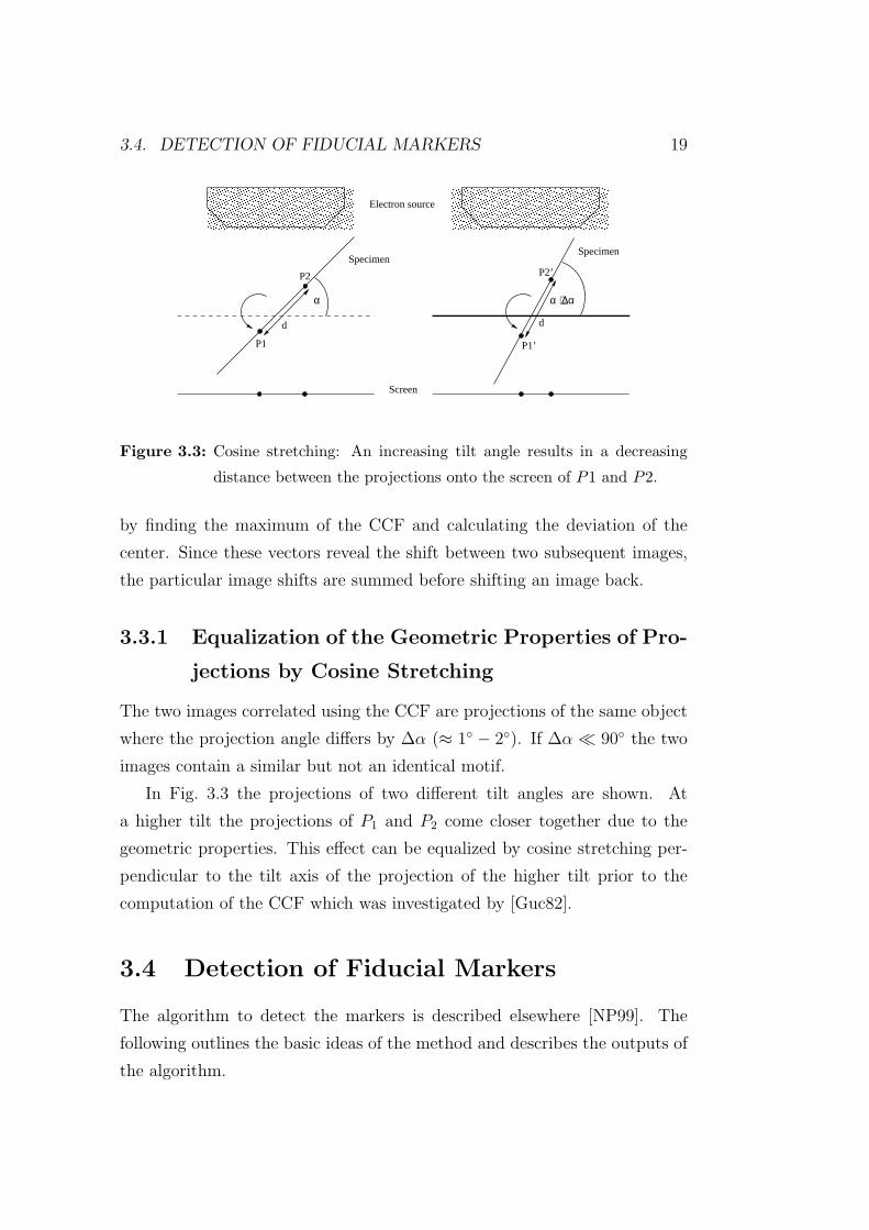
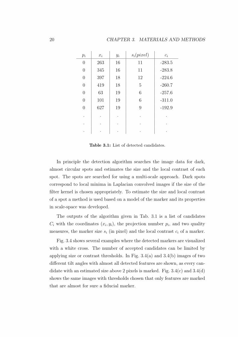
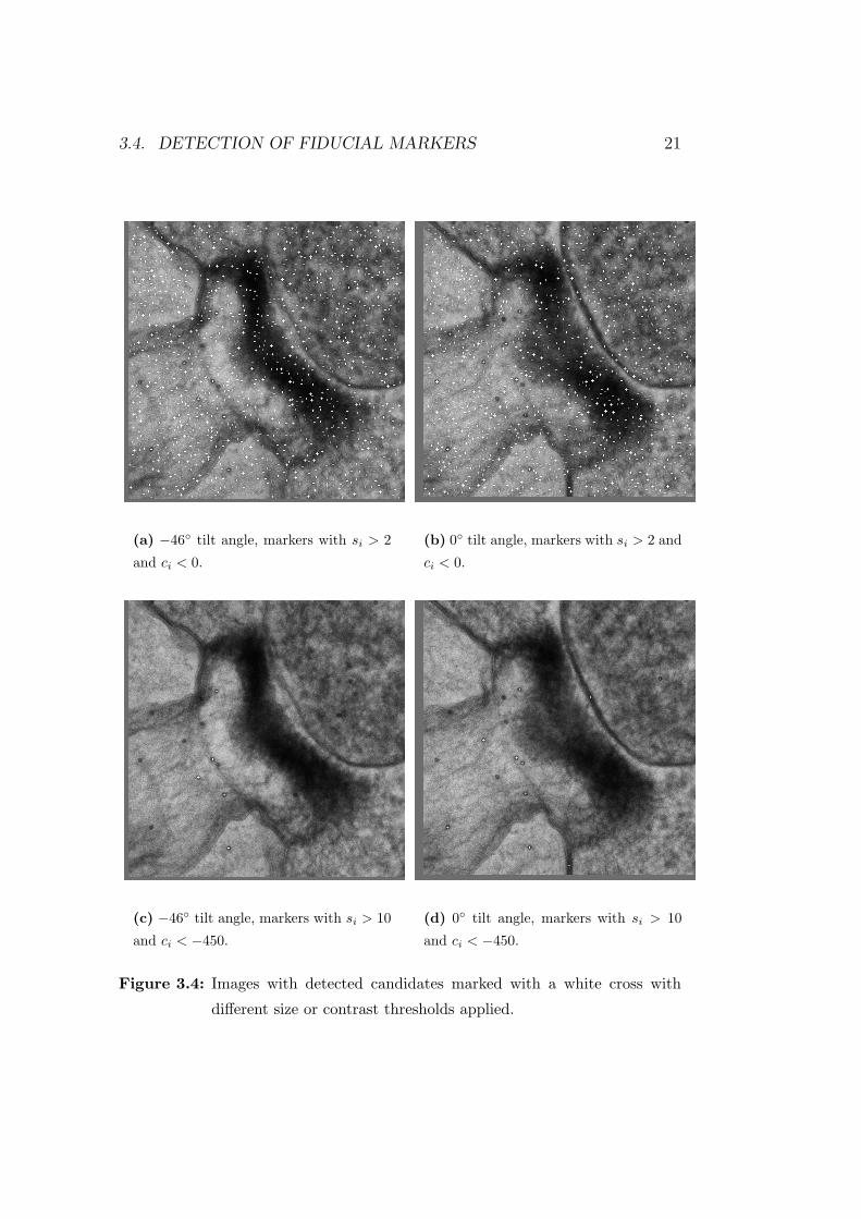
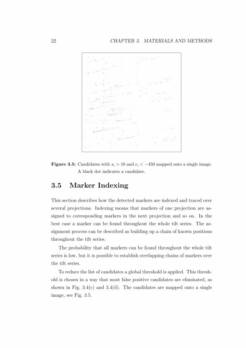


![Bayesian Inference and Experimental Design for Large ...is.tuebingen.mpg.de/.../files/publications/2010_09_25_final_[0].pdf · Eine Reihe empirischer Experimente ermittelt den EP-Algorithmus](https://static.unterlagen.site/doc/80x56/5e02f143d9e2ea2f20410344/bayesian-inference-and-experimental-design-for-large-is-0pdf-eine-reihe.jpg)


