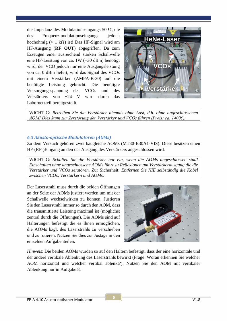
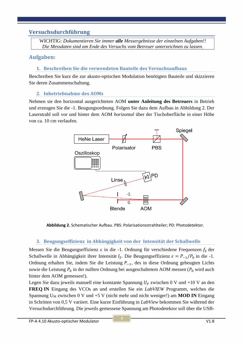
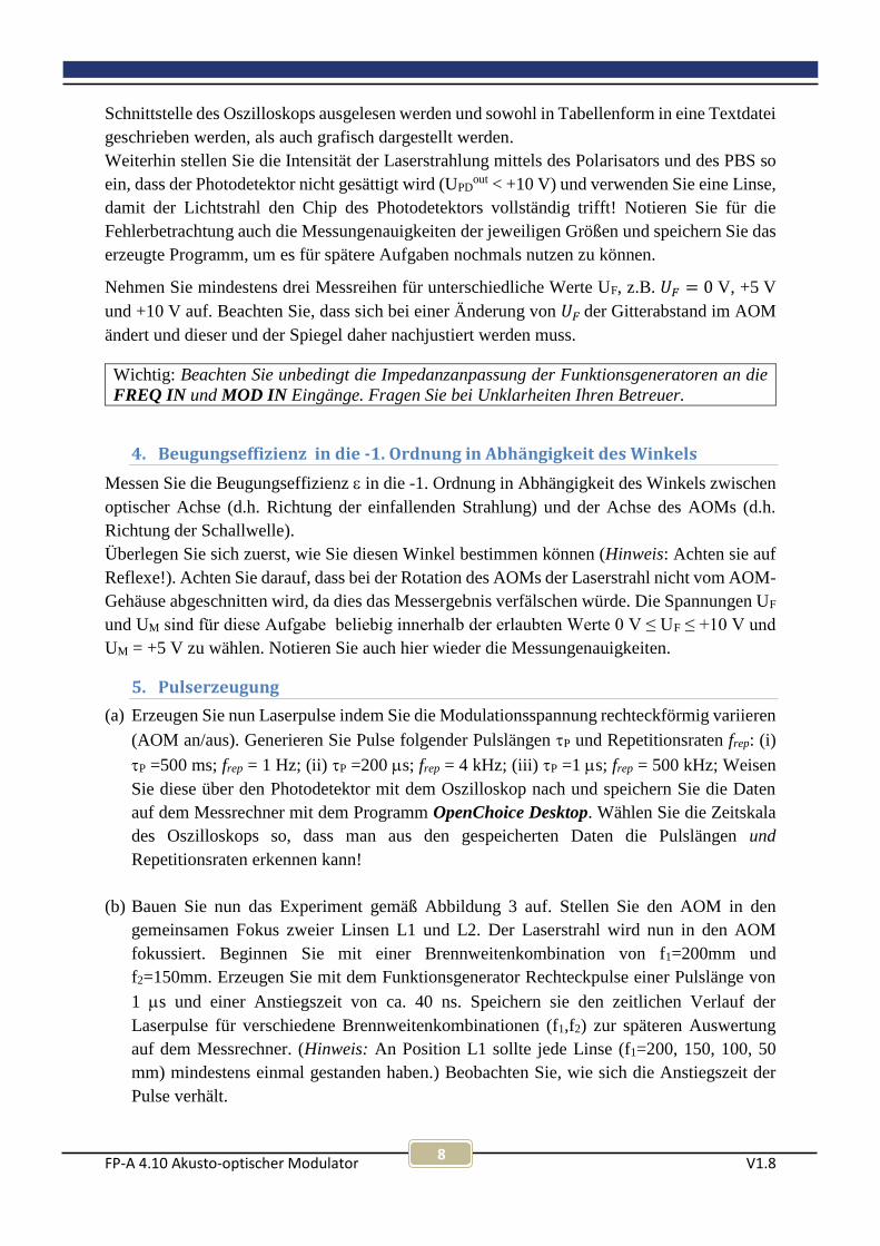
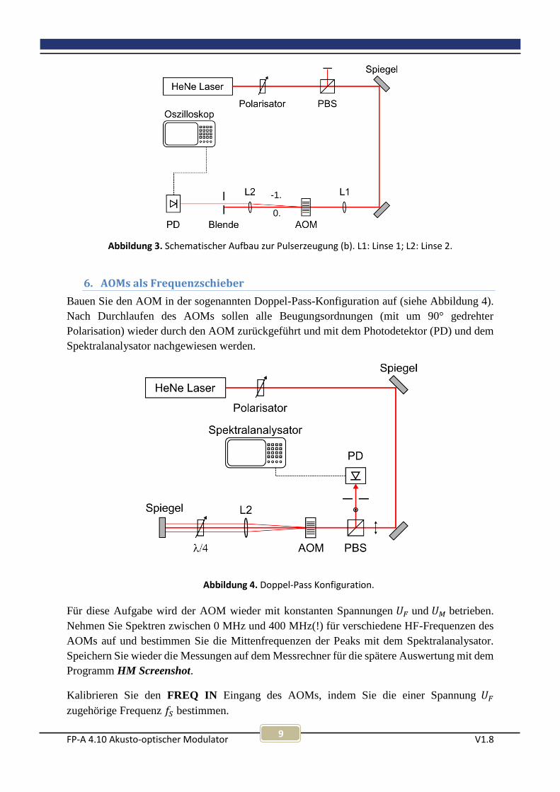
FP-A 4.10 Akusto-optischer Modulator V1.8 1 Akusto-optischer Modulator Fortgeschrittenenpraktikum A 4.10 t Fachbereich Physik Institut für Angewandte Physik AG Nichtlineare Optik / Quantenoptik T. Halfmann
Transcript
FP-A 4.10 Akusto-optischer Modulator V1.8
1
Akusto-optischer Modulator
Fortgeschrittenenpraktikum A 4.10
t
Fachbereich Physik
Institut für Angewandte Physik
AG Nichtlineare Optik / Quantenoptik
T. Halfmann
FP-A 4.10 Akusto-optischer Modulator V1.8
2
Vorbereitung
Lesen Sie die Versuchsanleitung aufmerksam durch und machen Sie sich mit der
prinzipiellen Bedienung der einzelnen verwendeten Geräte vertraut!
Informieren Sie sich über folgende Themengebiete:
Akusto-optischer Effekt & Funktionsweise eines AOM
Beugung am Gitter
Beugungseffizienz in Abhängigkeit der Intensität der Schallwellen
Schaltzeit eines AOM
Betriebsregime eines AOM
Impedanz-Anpassung
AOMs in Doppelpass-Konfiguration (siehe Paper in Versuchsanleitung)
Schwebung von Schwingungen nahezu gleicher Frequenzen
Lissajous-Figuren
Gefahren durch Laserstrahlung (siehe z.B. Wikipedia)
Literatur
1. Robert D. Guenther, Encyclopedia of Modern Optics, Wiley, New York (1990)
2. Frank L. Pedrotti, Leno S. Pedrotti, Werner Bausch, Hartmut Schmidt, Optik für
Ingenieure, Springer Verlag, 4. Auflage (2007)
3. Eine Übersicht (in Englisch) finden Sie bspw. auch auf den Herstellerseiten von
AA Opto-Electronic unter „Theory & general application notes“, sowie Brimrose.
4. W. Demtröder, Experimentalphysik 2, Springer Verlag
3.) Versuchsdurchführung (inkl. der aufgenommenen Messdaten) und Auswertung der
einzelnen Messaufgaben
4.) Fazit
Es muss nachvollziehbar sein, wie die Auswertungsergebnisse aus den Messdaten erhalten
wurden! Beschreiben Sie die Auswertung der einzelnen Aufgaben unmittelbar nach der
dazugehörigen Durchführung!
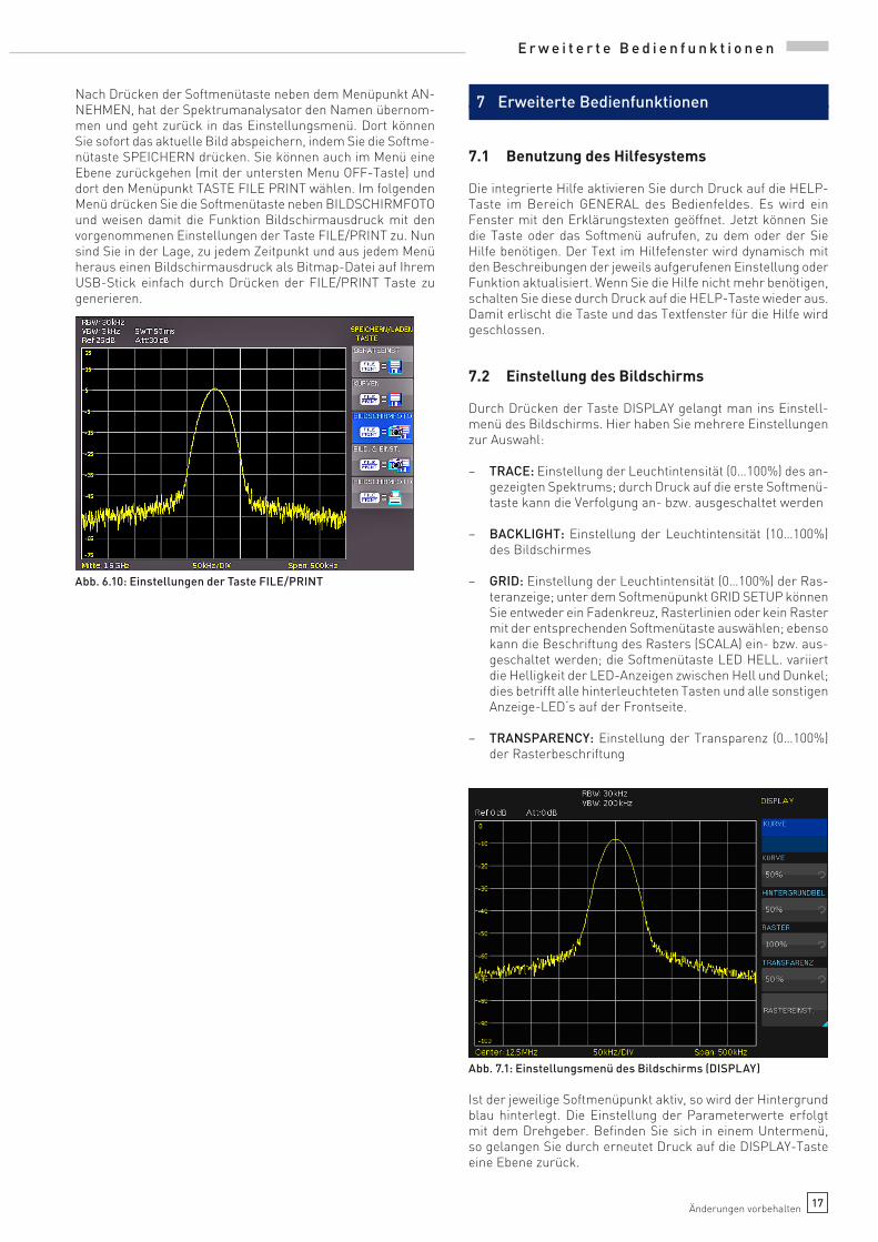
1. Tragen Sie die mit Einfach-Pass-Konfiguration gemessenen Beugungseffizienzen in die
-1. Ordnung bei verschiedenen HF-Frequenzen zusammen gegenüber der
Kontrollspannung 𝑈𝑀 auf und vergleichen Sie die jeweiligen Messreihen untereinander
und mit dem theoretischen Verlauf.
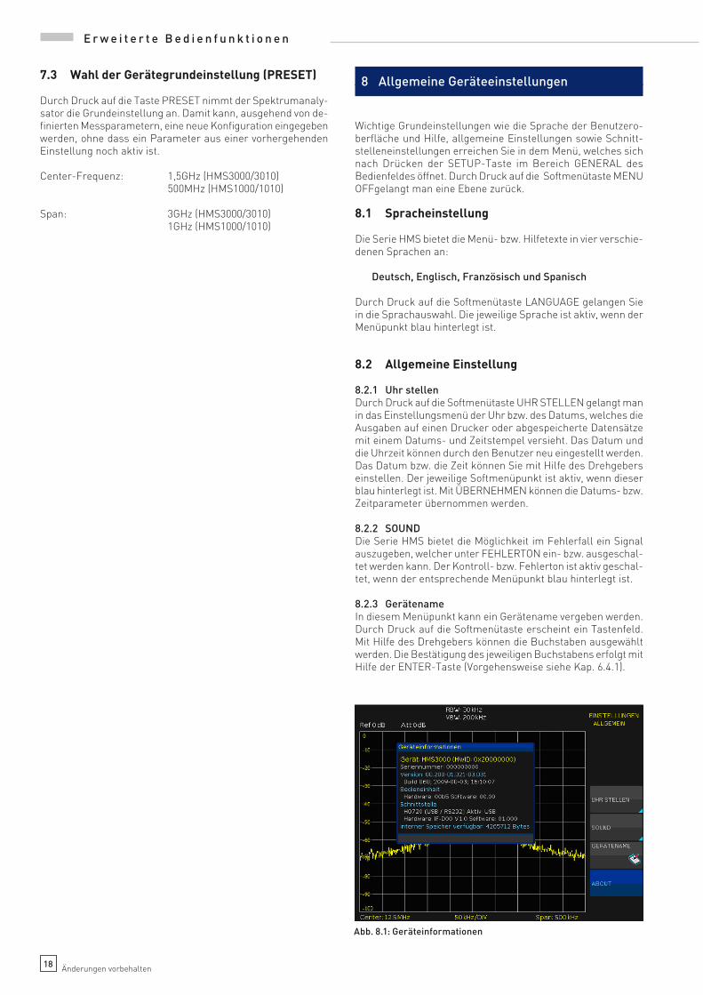
2. Tragen Sie die Beugungseffizienz in die -1. Ordnung in Abhängigkeit vom Winkel
zwischen optischer Achse und der Achse des AOM in einem Diagramm auf. Geben Sie
auch hier Fehlerbalken an. Bestimmen Sie den Braggwinkel für die gewählte
Kontrollspannung 𝑈𝐹 .
3. Werten Sie die in Aufgabe 5 gemessenen Pulsverläufe bzgl. ihrer Anstiegszeit für
verschiedene Linsen aus (Hinweis: Die tanh(t) Funktion könnte sich hier als nützlich
erweisen). Diskutieren Sie die Ergebnisse – auch im Hinblick auf die Erwartung laut
Theorie. Vergleichen sie die gemessenen Anstiegszeiten mit der Anstiegszeit laut
Spezifikation des AOMs.
4. Diskutieren Sie den Ursprung der Peaks innerhalb des in Aufgabe 6 aufgenommenen
Gesamtspektrums (0-400 MHz).
5. Kalibrieren Sie die Kontrollspannung UF. Tragen Sie hierfür die gemessene Frequenz
der Schallwelle gegen die Spannung UF in einem Diagramm auf. Geben Sie auch
Fehlerbalken an.
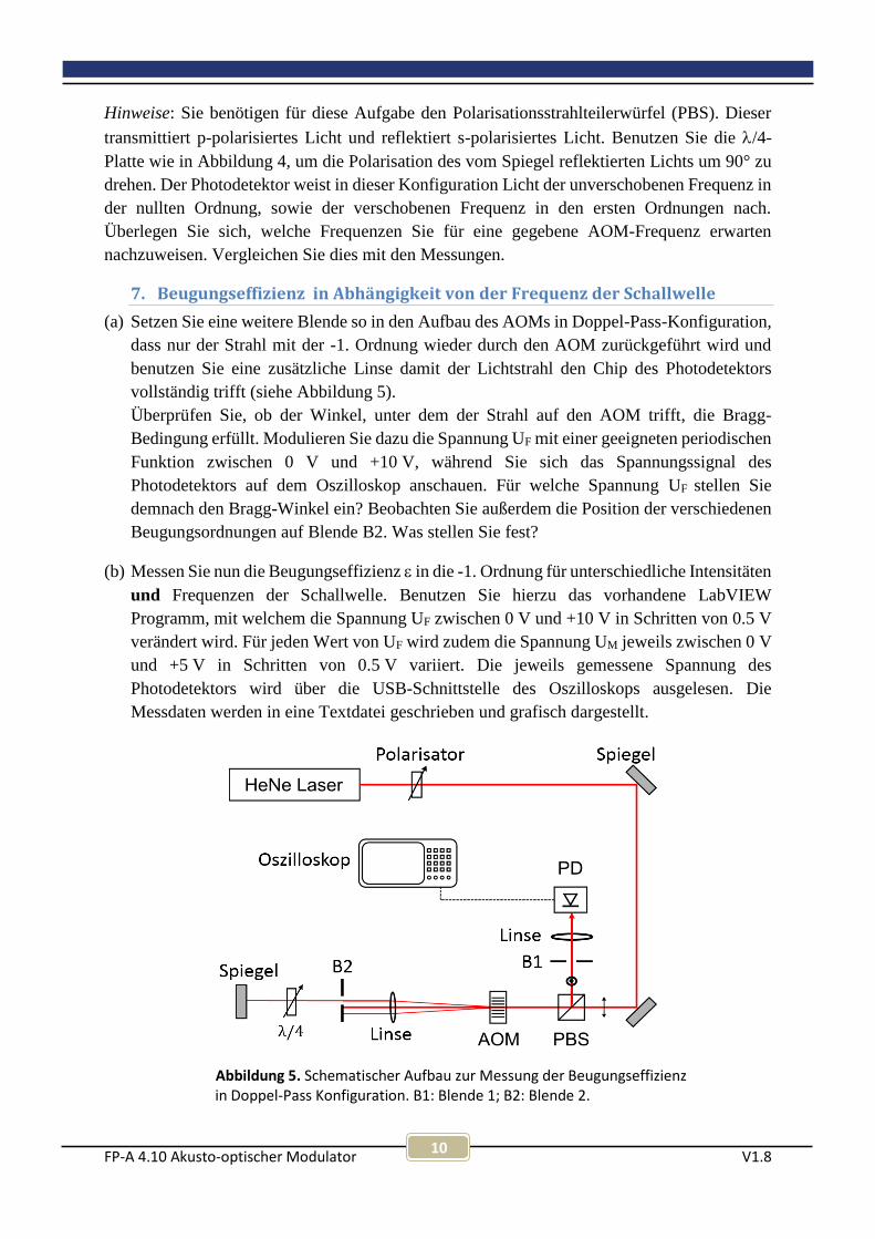
6. Stellen Sie die in Doppel-Pass-Konfiguration gemessenen Beugungseffizienzen in die
-1. Ordnung als Kontourplot gegenüber der Kontrollspannung 𝑈𝑀 und der HF-Frequenz
dar. Rechnen Sie hierfür die Kontrollspannung 𝑈𝐹 in die HF-Frequenz um (siehe 5.).
Beschreiben Sie das Verhalten der Beugungseffizienz. Welche Bedeutung hat dies für
die praktische Verwendung von AOMs?
7. Berechnen Sie aus zuvor gemessenen Größen die Schallgeschwindigkeit im Kristall
inkl. des Fehlers.
8. Diskutieren und begründen Sie, in welchem Regime die AOMs dieses Versuchs
betrieben werden: Bragg oder Raman-Nath?
FP-A 4.10 Akusto-optischer Modulator V1.8
13
Wichtige Punkte zum Laserschutz
Ganz allgemein gilt: Im Umgang mit Lasern ist der gesunde Menschenverstand nicht
zu ersetzen! Einige spezielle Hinweise werden im Folgenden angeführt.
1. Die Laserschutzvorschriften sind immer zu beachten.
2. Halten Sie Ihren Kopf niemals auf Strahlhöhe.
3. Die Justierbrille immer aufsetzen.
4. Schauen Sie nie direkt in Strahl – auch nicht mit Justierbrille!
5. Achtung: praktisch alle Laser für Laboranwendungen sind mindestens Klasse 3, also
von vornherein für die Augen gefährlich, ggf. auch für die Haut – evtl.
auch hierfür Schutzmaßnahmen ergreifen. Zur Justage kann der Laserstrahl mittels
einem Stück Papier sichtbar gemacht werden.
6. Auch Kameras besitzen eine Zerstörschwelle!
7. Spiegel und sonstige Komponenten nie in den ungeblockten Laserstrahl einbauen! Vor
Einbau immer überlegen, in welche Richtung der Reflex geht! Diese Richtung zunächst
blocken, bevor der Strahl wieder frei gegeben wird.
8. Nie mit reflektierenden Werkzeugen im Strahlengang hantieren! Unkontrollierbare
Reflexe! Vorsicht ist z.B. auch mit BNC-Kabeln geboten, die in den Strahlengang
gelangen könnten! Gleiches gilt auch für Uhren und Ringe. Diese vorsichtshalber
ausziehen, wenn Sie mit den Händen im Strahlengang arbeiten.
9. Auch Leistungsmessgeräte können Reflexe verursachen! Unbeschichtete
Silizium-Fotodioden reflektieren über 30% des Lichtes!
10. Achtung im Umgang mit Strahlteilerwürfeln! Diese haben immer einen zweiten
Ausgang! Ggf. abblocken!
11. Warnlampen bei Betrieb des Lasers anschalten und nach Beendigung der Arbeit wieder
ausschalten.
12. Dafür sorgen, dass auch Dritte im Labor die richtigen Schutzbrillen tragen, oder sich
außerhalb des Laserschutzbereiches befinden.
13. Filtergläser in Laserschutzbrillen dürfen grundsätzlich nicht aus- oder umgebaut
werden!!!
14. In besonderem Maße auf Beistehende achten.
15. Optiken (Linsen, Spiegel etc.) nicht direkt mit den Fingern berühren!
Hiermit erkläre ich, dass ich die vorstehenden Punkte gelesen und verstanden habe. Ich
bestätige, dass ich eine Einführung in den Umgang mit Lasern sowie eine arbeitsplatzbezogene
Unterweisung erhalten habe.
Name:
Unterschrift: Datum:
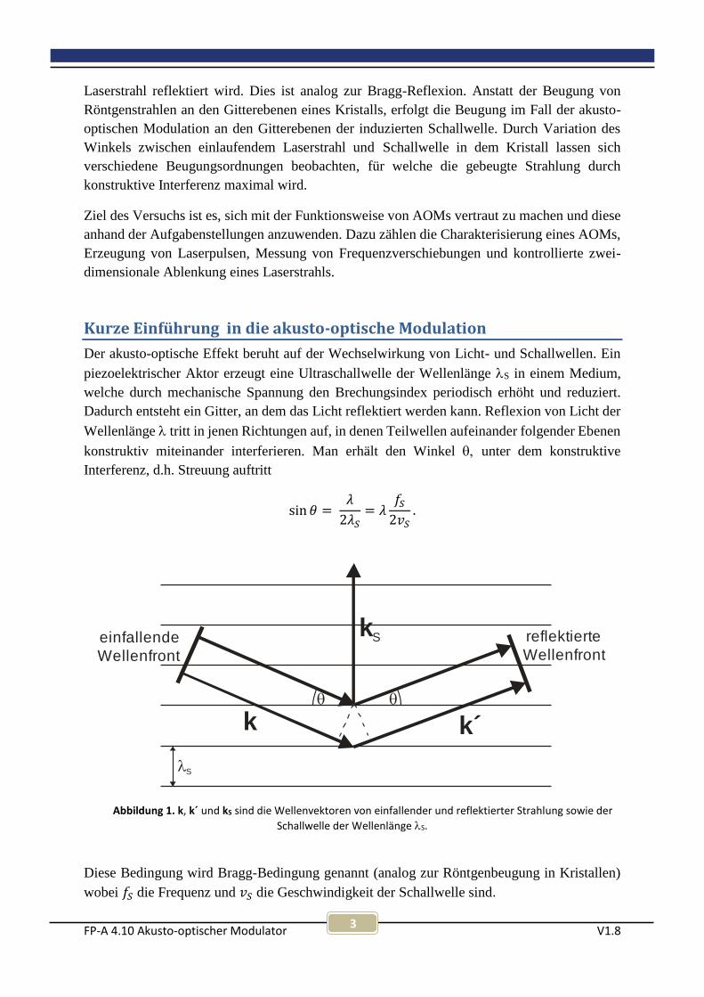
Criterion for Bragg and Raman-Nathdiffraction regimes
M. G. Moharam and L. Young
The idea is well entrenched in the literature that thin phase gratings (whether holographic or acoustically in-
duced) should exhibit Raman-Nath behavior (and thus give several diffracted waves), and that thick phasegratings should show Bragg behavior (one diffracted beam and that only for Bragg angle incidence). The
parameter Q of Klein and Cook, which is a normalized measure of grating thickness, has been extensively
used as a criterion for deciding which regime will apply. It is perhaps not generally realized that Q is not a
reliable parameter for this purpose but requires, as indeed Klein and Cook noted, a limitation on gratingstrength. This limitation is a matter of practical concern. For example, we have observed Raman-Nath
behavior with Fe-doped LiNbO3 even for very large values of Q. The purpose of the present paper is to note
that a parameter p (first defined by Nath) is an effective replacement for Q, since p is reliable and Q is not.
p is defined as X02/A2nonI, where Xo is the vacuum wavelength of the light, A is the grating spacing, no is the
mean refractive index, and nj is the amplitude of the sinusoidal modulation of the refractive index. Thegrating thickness does not enter p, so the terms thin and thick are, strictly speaking, irrelevant to the ques-tion of which regime is operative. However, thin enough gratings will tend to operate in the Raman-Nath
regime because the index modulation must be large for a thin grating to produce appreciable diffraction.
Introduction
The phenomenon of light diffraction by periodicphase gratings, whether holographically or acousticallyproduced, has been treated extensively by many au-thors.1-15 There is general agreement that it is conve-nient to define two regimes in which phase gratingsoperate. In the Raman-Nath regime, several diffractedwaves are produced. In the Bragg regime, essentiallyonly one diffracted wave is produced, and that only fornear Bragg incidence. It has been customary to referto gratings which operate in the Raman-Nath or theBragg regimes as thin and thick gratings, respectively.Klein and Cook4 introduced a parameter Q, defined as2 7rXoL/A2no (where L is the grating thickness, X0 is thevacuum wavelength of light, A is the grating spacing,and no is the mean refractive index) to distinguish be-tween the two diffraction regimes. Values of Q < 1, i.e.,thin gratings, were believed to give Raman-Nath oper-ation. Large values of Q (Q > 10), i.e., thick gratings,were believed to give Bragg regime operation. The useof Q is well entrenched in the literature. However, as
The authors are with University of British Columbia, ElectricalEngineering Department, Vancouver, B.C., V6T 1W5.
Received 30 November 1977.0003-6935/78/0601-1757$0.50/0.() 1978 Optical Society of America.
Klein and Cook noted, their analysis was based on theassumption that v = 27rnL/Xo remains less than six;and if v exceeds this value, it is necessary to place morerestrictive conditions on Q (which they proceeded todiscuss). Actually, it can be shown that Q may fail withv as low as three. Recently, Magnusson and Gaylord 8
have shown theoretically that for a large modulation,higher order diffracted waves become important(Raman-Nath regime) even for large Q. Conversely,for small modulation, only a single wave is diffracted inspite of small values of Q. Kaspar 7 came to a similarconclusion when he compared his theory for a gratingwith a complex dielectric constant with the coupledwave theory of Kogelnik. 3 Alferness 9 has discussedqualitatively the effect of the magnitude of the modu-lation of the refractive index on the validity of Q as atool to predict the regime of diffraction. Various au-thors8 9"16 have observed several diffracted waves duringhologram recording in lithium niobate and dichromatedgelatine when Q was large. We have observed up toeight diffracted waves during hologram storage in 1-cmthick Fe-doped lithium niobate crystal. For this ex-periment, Q = 55.
These experimental observations, in addition to thetheoretical predictions which show that Q does notwork, led us to reconsider the basis of the use of Q andto seek to find a parameter which could be used to pre-dict the regime of diffraction. We will show that a pa-rameter p defined as Xo2/A2non, (where n1 is the mod-
ulation of the refractive index and Ao, A, and no are asdefined before) can be reliably used to predict whetherone is in the Raman-Nath regime or in the Bragg regime.The parameter p was defined first by Nath,1 2 who wasconsidering the case of normal incidence. Nath pointedout that, if p is very large, the diffraction effect will notbe prominent, as is otherwise the case where p is nearlyzero. Phariseau13 and later Bergstein and Kermisch5
and Chu and Tamir 6 have obtained expressions for theintensities of the first few diffracted orders near the firstBragg incidence 5"13 and higher order Bragg angle 6 as-suming that p is large (Bergstein and Kermisch5 andChu and Tamir 6 defined a parameter equal to 1/p calleds and q in successive papers.) Those authors 5 6"13 haveused p >> 1 (or 1/p << 1) in mathematical approximationsto obtain analytical expressions of the intensities. Theydid not use it to predict whether one is in the Raman-Nath or the Bragg regime. In fact, they did not addresseither the problem of determining the diffraction regimeor the problem of the effectiveness of Q in distinguishingbetween the two regimes.
Theory
The problem of light diffraction by periodic phasegratings has, of course, been treated in detail in manypapers.'- 1 5 We will only give a brief outline here.
The scalar wave equation is
V2E + k2E=0O (1)
where k2= 32 - jat and E(x,z,t) is the complex am-
plitude of the y component of the field. = 27rn/X isthe propagation constant, and n is the refractive index.A sinusoidal modulation of the refractive index is as-sumed.
n = no + n cos(2rx/A). (2)
Here, no, ni, XO, and A are as defined before. An un-slanted grating is assumed for simplicity. The electricfield E may be represented by its Fourier expansionas
E E z(z) exp(-jia .), (3)
where - = o - 1K, where K is the grating vector andK = 27r/A, Uo is the wave vector of the incident wave (1= 0), and = (x,y,z).
Substituting Eqs. (2) and (3) in Eq. (1) and neglectingthe second derivative with respect to z, we arrive at thewell'known set of coupled wave equations:
jpl2(1 - B)O + j(0- + 01+1), (4)
where B = 2A sinOo/Xol, O is the external angle of inci-dence, = v(z/L), v = rnL/Xo cosOl, and 0 is the angleof diffraction of the zero-order mode. Thus, B1 is equalto 1 for Bragg diffraction forming the th mode, and vis a measure of the grating strength (and appears, e.g.,in the coupled mode theory of Kogelnik for Bragg dif-fraction3). The absorption constant a may be neglectedwithout loss of generality since it can be allowed for bythe substitution 0i' = Oi exp(-az/cos0).
Equation (4) shows that the Ith mode is coupled toitself and to two adjacent modes ( - 1th and I + 1thmodes). Effective energy transfer between modes re-quires essentially that the factor pl 2 (1 - B) be relativelysmall since, if this factor is much larger than 1, almostall the energy will be coupled back to the th mode.[This can be seen from Eq. (1) by neglecting the secondterm of the right-hand side.] Therefore, if p < 1, ap-preciable energy may be transferred successfully tohigher order modes up to some value of I provided themagnitude of B1 is appropriately limited. The numberof higher order modes depends on how small p is. (Thesmaller p is, the larger the number of higher ordermodes.) If p = 0, Eq. (1) gives the well-known solutionin terms of Bessel functions oj = jlJI (2v). This solutionis often obtained by Fourier expansion of the trans-mitted wave with spatially sinusoidal phase modula-tions. A similar solution was shown by Klein and Cookfor Q = 0. However, as the thickness L of the gratinggoes to zero (Q - 0) the modulation of the refractiveindex must go to infinity to retain the finite phase shift(nL); and as n1 - a, p - 0. Clearly, the case where Qor p = 0 is a nonphysical situation. For p < 1, the dif-fraction process is in the Raman-Nath regime. If p >>1, appreciable energy may be transferred only into themode for which the Bragg conditions holds or nearlyholds, i.e., the mode with such that B1 1 for the given0. All the above applies to an infinite plane wave in-cident on an infinite grating, as in previous work.4
The above analysis was illustrated by solving the set
1, .
1.
0.5
0.0
L-
Uiz
z
05100
5 10 15 20 25GRATING STRENGTH (V)
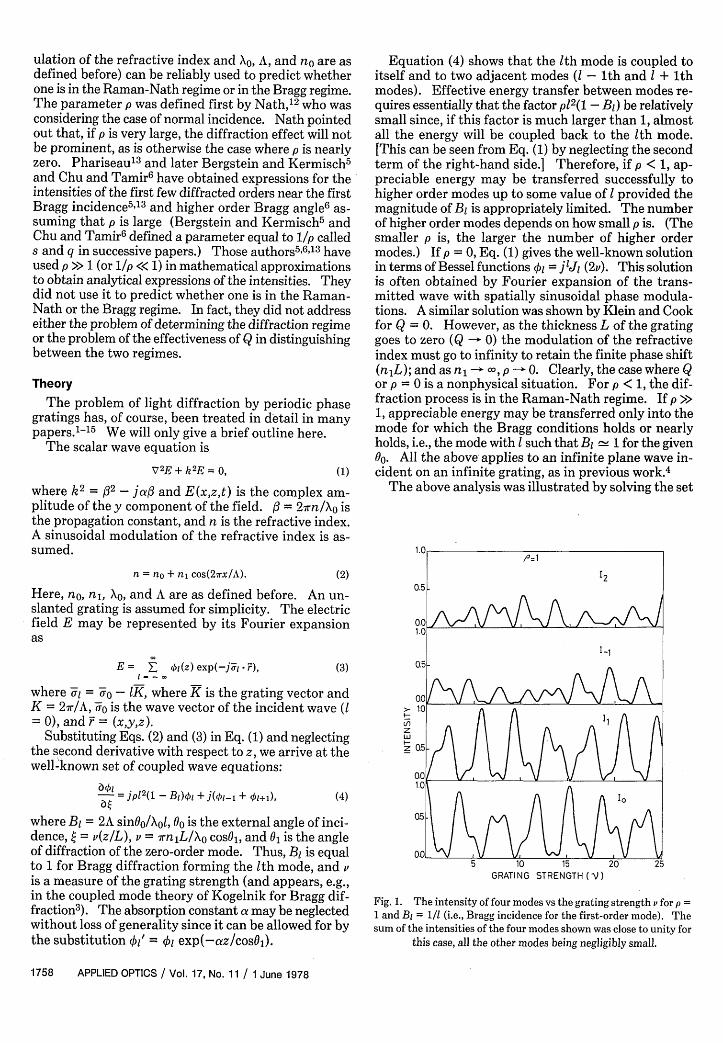
Fig. 1. The intensity of four modes vs the grating strength v for p =1 and B = 1/1 (i.e., Bragg incidence for the first-order mode). Thesum of the intensities of the four modes shown was close to unity for
this case, all the other modes being negligibly small.
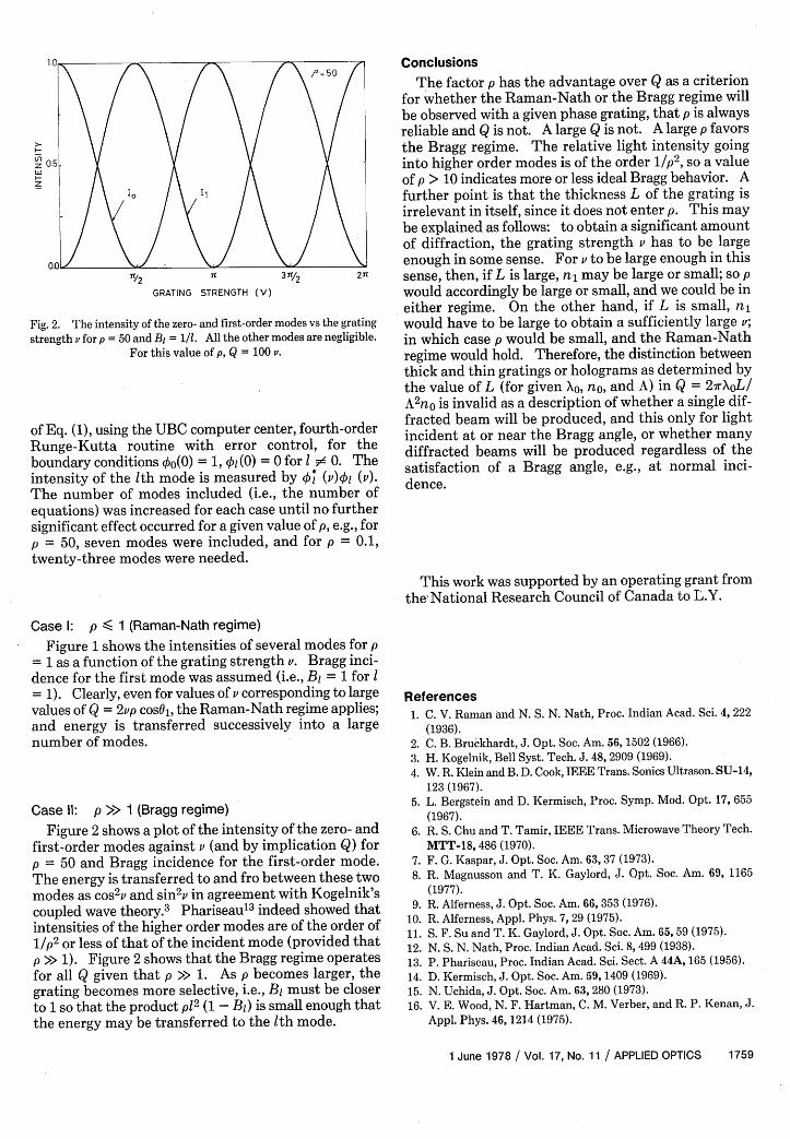
Fig. 2. The intensity of the zero- and first-order modes vs the grating
strength v for p = 50 and B, = 1/1. All the other modes are negligible.For this value of p, Q = 100 v.
of Eq. (1), using the UBC computer center, fourth-orderRunge-Kutta routine with error control, for theboundary conditions 4o(0) = 1, 01(0) = 0 for 1 s! 0. Theintensity of the lth mode is measured by 0* (v)01 (v).The number of modes included (i.e., the number ofequations) was increased for each case until no furthersignificant effect occurred for a given value of p, e.g., forp = 50, seven modes were included, and for p = 0.1,twenty-three modes were needed.
Case 1: p 1 (Raman-Nath regime)
Figure 1 shows the intensities of several modes for p= 1 as a function of the grating strength v. Bragg inci-dence for the first mode was assumed (i.e., B1 = 1 for 1= 1). Clearly, even for values of v corresponding to largevalues of Q = 2vp cos0j, the Raman-Nath regime applies;and energy is transferred successively into a largenumber of modes.
Case 11: p >> 1 (Bragg regime)
Figure 2 shows a plot of the intensity of the zero- andfirst-order modes against v (and by implication Q) forp = 50 and Bragg incidence for the first-order mode.The energy is transferred to and fro between these twomodes as cos2v and sin2v in agreement with Kogelnik'scoupled wave theory.3 Phariseau' 3 indeed showed thatintensities of the higher order modes are of the order of1/p2 or less of that of the incident mode (provided thatp >> 1). Figure 2 shows that the Bragg regime operatesfor all Q given that p >> 1. As p becomes larger, thegrating becomes more selective, i.e., BI must be closerto 1 so that the product p12 (1 - B) is small enough thatthe energy may be transferred to the 1th mode.
Conclusions
The factor p has the advantage over Q as a criterionfor whether the Raman-Nath or the Bragg regime willbe observed with a given phase grating, that p is alwaysreliable and Q is not. A large Q is not. A large p favorsthe Bragg regime. The relative light intensity goinginto higher order modes is of the order 1/p2 , so a valueof p > 10 indicates more or less ideal Bragg behavior. Afurther point is that the thickness L of the grating isirrelevant in itself, since it does not enter p. This maybe explained as follows: to obtain a significant amountof diffraction, the grating strength v has to be largeenough in some sense. For v to be large enough in thissense, then, if L is large, nj may be large or small; so pwould accordingly be large or small, and we could be ineither regime. On the other hand, if L is small, njwould have to be large to obtain a sufficiently large v;in which case p would be small, and the Raman-Nathregime would hold. Therefore, the distinction betweenthick and thin gratings or holograms as determined bythe value of L (for given Xo, no, and A) in Q = 27rXoL/A2 no is invalid as a description of whether a single dif-fracted beam will be produced, and this only for lightincident at or near the Bragg angle, or whether manydiffracted beams will be produced regardless of thesatisfaction of a Bragg angle, e.g., at normal inci-dence.
This work was supported by an operating grant fromthe National Research Council of Canada to L.Y.
References1. C. V. Raman and N. S. N. Nath, Proc. Indian Acad. Sci. 4, 222
(1936).2. C. B. Bruckhardt, J. Opt. Soc. Am. 56, 1502 (1966).3. H. Kogelnik, Bell Syst. Tech. J. 48, 2909 (1969).4. W. R. Klein and B. D. Cook, IEEE Trans. Sonics Ultrason. SU-14,
123 (1967).5. L. Bergstein and D. Kermisch, Proc. Symp. Mod. Opt. 17, 655
(1967).6. R. S. Chu and T. Tamir, IEEE Trans. Microwave Theory Tech.
MTT-18, 486 (1970).7. F. G. Kaspar, J. Opt. Soc. Am. 63, 37 (1973).8. R. Magnusson and T. K. Gaylord, J. Opt. Soc. Am. 69, 1165
(1977).9. R. Alferness, J. Opt. Soc. Am. 66, 353 (1976).
10. R. Alferness, Appl. Phys. 7, 29 (1975).11. S. F. Su and T. K. Gaylord, J. Opt. Soc. Am. 65, 59 (1975).
12. N. S. N. Nath, Proc. Indian Acad. Sci. 8, 499 (1938).13. P. Phariseau, Proc. Indian Acad. Sci. Sect. A 44A, 165 (1956).14. D. Kermisch, J. Opt. Soc. Am. 59, 1409 (1969).15. N. Uchida, J. Opt. Soc. Am. 63, 280 (1973).16. V. E. Wood, N. F. Hartman, C. M. Verber, and R. P. Kenan, J.
Double-pass acousto-optic modulator systemE. A. Donley,a! T. P. Heavner, F. Levi,b! M. O. Tataw, and S. R. JeffertsTime and Frequency Division, National Institute of Standards and Technology, 325 Broadway, Boulder,Colorado 80305
sReceived 2 March 2005; accepted 21 April 2005; published online 1 June 2005d
A practical problem that arises when using acousto-optic modulatorssAOMsd to scan the laserfrequency is the dependence of the beam diffraction angle on the modulation frequency. Alignmentproblems with AOM-modulated laser beams can be effectively eliminated by using the AOM in thedouble-pass configuration, which compensates for beam deflections. On a second pass through theAOM, the beam with its polarization rotated by 90° is deflected back such that it counterpropagatesthe incident laser beam and it can be separated from the input beam with a polarizing beam splitter.Here we present our design for a compact, stable, double-pass AOM with 75% double-passdiffraction efficiency and a tuning bandwidth of 68 MHz full width at half maximum for lighttransmitted through a single-mode fiber. The overall efficiency of the systemsdefined as the opticalpower out of the single-mode fiber divided by the optical power into the apparatusd is 60%.fDOI: 10.1063/1.1930095g
I. INTRODUCTION
For many laser cooling and trapping experiments, it isnecessary to shift and/or sweep the laser frequency at the endof a cooling cycle. This is done to either adiabatically coolthe atoms to a lower temperature, or to manipulate them insome other way, such as launching them in an atomic foun-tain. Most often, the laser frequency must be switched ontime scales shorter than 1 ms, and it may be that laser beamswith several different frequencies must be produced from asingle laser source.
Acousto-optic modulatorssAOMsd are widely used toaccomplish the frequency control in laser cooling experi-ments. When the laser frequency is scanned with an AOM,the angle of the first-order diffracted beam shifts as well,since the beam diffraction angle is a function of modulationfrequency. Changes in beam diffraction angle may be desir-able for some applications where spatially resolved dif-fracted beams are needed, but for many applications anychange in the laser propagation direction is an unwanted sideeffect. Using an AOM in the double-pass configuration is away to practically eliminate changes in beam steering duringfrequency sweeps and jumps within the frequency tuningbandwidth of the AOM. Here we present a detailed descrip-tion of our modular double-pass system design and a studyof the system’s performance.
The article is organized as follows. In Sec. II, the laserfrequency jump and ramp sequence that is used to cool andlaunch the atoms in the primary frequency standard at theNational Institute of Standards and TechnologysNISTd ispresented in detail. This provides a real-world example of thelevel of laser frequency control that can be desirable for
atomic physics experiments. In Sec. III, background into theproperties of acousto-optic modulators is presented. In Sec.IV, the double-pass configuration is introduced, our specificdesign is discussed in detail, and the performance of ourdesign is presented.
II. ATOMIC FOUNTAIN LASER FREQUENCYCONTROL
For laser cooling and trapping experiments, the optimumlaser intensity and detuning values that maximize the numberof laser-cooled atoms are not the same as the optimum valuesfor the lowest atom temperature. The laser intensity thatmaximizes the number of atoms can depend on the details ofthe atom source, but in general, a higher laser intensity isbetter for a thermal source. The optimum laser detuning isgenerally a few linewidths, but it can also depend on thedetails of the atom source and the laser intensity. In contrast,at low laser intensities the equilibrium atom temperature inan optical molasses is equal to a small constant terms,1 mK for 133Csd plus a term that is proportional to thelaser intensity and inversely proportional to the laserdetuning.1,2 To simultaneously maximize the atom numberand minimize the atom temperature, often a brief “postcool”stage is applied as the molasses is turned off. During thepostcool stage, the laser frequency is ramped further to thered of the atomic resonance while the intensity is ramped tozero.
The atom launch and postcool sequence for the verticallaser beams used in the NIST-F1 atomic fountain clock atNIST is shown in Fig. 1. NIST-F1 serves as the primaryfrequency standard for the United States, and a detailed de-scription of the apparatus has been published previously.3 Weaccomplish the frequency sweeps and jumps shown in Fig. 1with AOMs. The intensity ramp is produced by controllingthe rf power into the AOM with a voltage-controlled attenu-ator. With this sequence, we are able to collect about 107
adAuthor to whom correspondence should be addressed; electronic mail:[email protected]
atoms per cycle, cool them to,0.5 mK, and launch theminto a microwave cavity structure for Ramsey interrogation.
III. ACOUSTO-OPTIC MODULATORS
A. Bragg scattering
For most practical applications of acousto-optic modula-tors, the Bragg description of the modulation process is agood approximation to the behavior of the system.4,5 Themain features of AOMs are derived in this picture by treatingthe modulation as a photon-phonon scattering process.
The Bragg matching condition can be derived by treatingthe acoustic and optical fields as particles with momentumkandk, respectively, wherek skd is the phononsphotond wavevector for the acousticsopticald field; k=V /vs, whereV isthe rf modulation frequency andvs is the speed of sound inthe crystal. Similarly,k=v /vL, where v is the light fre-quency andvL is the speed of light in the crystal.
A scattering process between photons and phonons re-sults in the absorption or emission of acoustic phonons. Afirst-order scattering process between a photon and a singlephonon is described by the energy-momentum relations
vd = vi ± V,
kd = ki ± k. s1d
The subscriptsi andd designate whether the correspondingphoton is incident or diffracted. The sign depends on whetherthe phonon is absorbed or emitted, which depends on therelative orientations of the incident photon and phonon wavevectors.
The Bragg matching condition that determines the opti-mum angles for the incident laser and acoustic beams forpeak first-order diffraction efficiency can be derived withenergy and momentum conservation arguments. Figure 2
shows momentum conservation diagrams that describephoton-phonon scattering events in which a phonon is ab-sorbeds+first-order diffractiond. The photon momentum ofthe diffracted light is equal to the sum of the momenta of thephonon and the incident photon. Conservation of energy re-quires that the frequency of the diffracted beam be shiftedupward fromv to v+V for a phonon absorption process; butsincev@V, the frequency shift can be ignored in the mo-mentum conservation analysis, andukiu= ukdu. Adding togetherthex andy momentum components leads one to Bragg’s law
sinuB =k
2 ·ki, s2d
whereuB is the Bragg angle, andui =ud=uB. Note that wehave derived Eq.s2d without considering the effect of theboundaries of the acoustic medium. Often it is desirable tocalculate the Bragg angle outside of the crystal,uB,ext. Toclose approximation, if the crystal boundaries are parallel tok, the external Bragg angle is larger than the internal Braggangle by a factor ofn, wheren is the refractive index of theacoustic medium.
The cases shown in Figs. 2sad and 2sbd represent the twogeometries where the Bragg matching condition is met for+first-order phonon absorption for a given orientation ofk.Notice that the incident photon wave vector for one case andthe diffracted photon wave vector for the other case counter-propagate. This point is relevant to the discussion of thedouble-pass configuration below. Diagrams similar to thosein Fig. 2 can be drawn for the single-phonon emission pro-cess, where the diffracted light enters the −first order, andthe frequency of the diffracted beam is shifted tov−V.
B. Acousto-optic devices
A schematic drawing of an acousto-optic modulator isshown in Fig. 3. A rf signal is fed to a strain transducer incontact with the AOM crystal. The rf modulation at fre-quencyV causes a traveling density wave to form inside thecrystal; the wave propagates at the speed of sound in thecrystal, vs, with the frequencyV. The refractive index istherefore modulated with a wavelength ofL=2p ·vs/V, andthe crystal acts like a thick diffraction grating with the rul-ings traveling away from the transducer with a velocityvs.The Bragg approximation is valid only when the acousticwave is describable by a plane wave and all phonons have
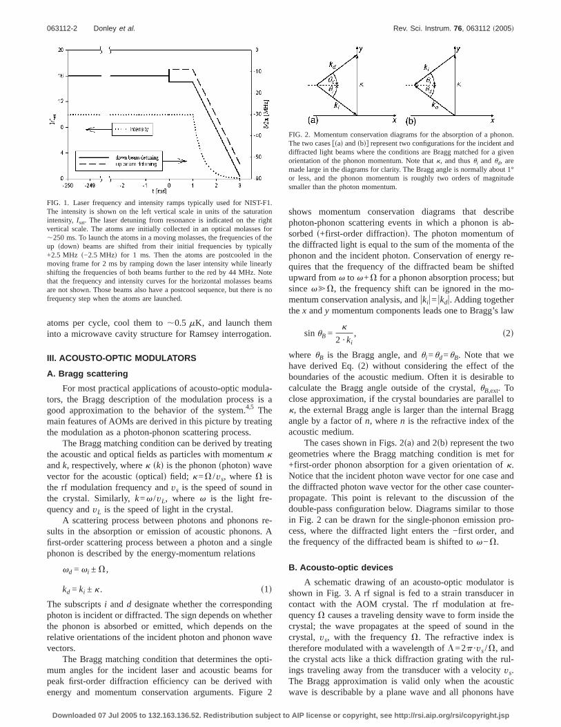
FIG. 1. Laser frequency and intensity ramps typically used for NIST-F1.The intensity is shown on the left vertical scale in units of the saturationintensity, Isat. The laser detuning from resonance is indicated on the rightvertical scale. The atoms are initially collected in an optical molasses for,250 ms. To launch the atoms in a moving molasses, the frequencies of theup sdownd beams are shifted from their initial frequencies by typically+2.5 MHz s−2.5 MHzd for 1 ms. Then the atoms are postcooled in themoving frame for 2 ms by ramping down the laser intensity while linearlyshifting the frequencies of both beams further to the red by 44 MHz. Notethat the frequency and intensity curves for the horizontal molasses beamsare not shown. Those beams also have a postcool sequence, but there is nofrequency step when the atoms are launched.
FIG. 2. Momentum conservation diagrams for the absorption of a phonon.The two casesfsad andsbdg represent two configurations for the incident anddiffracted light beams where the conditions are Bragg matched for a givenorientation of the phonon momentum. Note thatk, and thusui and ud, aremade large in the diagrams for clarity. The Bragg angle is normally about 1°or less, and the phonon momentum is roughly two orders of magnitudesmaller than the photon momentum.
063112-2 Donley et al. Rev. Sci. Instrum. 76, 063112 ~2005!
Downloaded 07 Jul 2005 to 132.163.136.52. Redistribution subject to AIP license or copyright, see http://rsi.aip.org/rsi/copyright.jsp
the same wave vector. In practice, this limiting case can beachieved to a close approximation when the strain transduceris long compared to the acoustic wavelength in the directionof laser beam propagation and acoustic diffraction is mini-mized. It is therefore not uncommon to achieve greater than80% diffraction efficiency into a single diffraction order withcareful engineering.5 The AOM that we usesCrystal Tech-nology, Inc. 3080-120d6 has a TeO2 crystal driven with alongitudinal acoustic mode. At a typical rf frequency of 80MHz the external Bragg angle is 8 mrad for light with avacuum wavelength of 852 nm.
C. Bandwidth
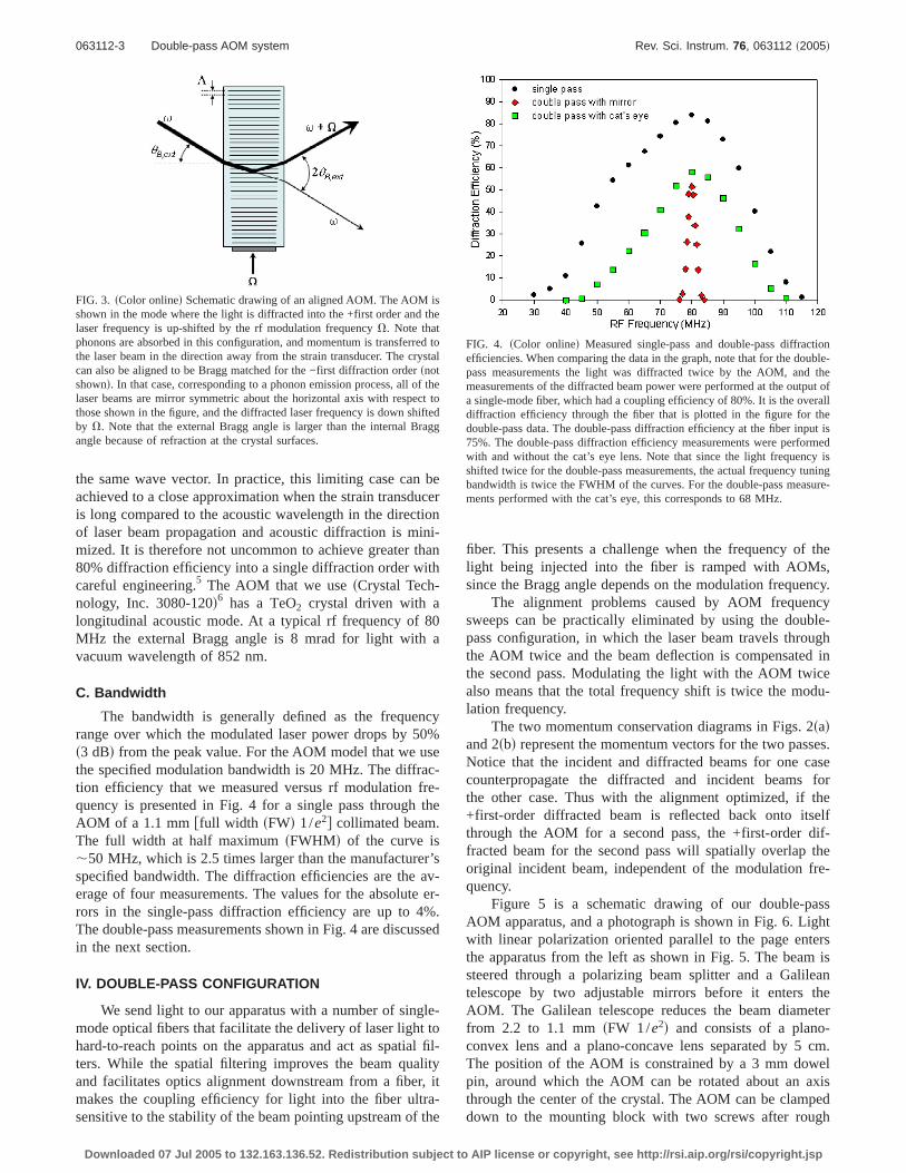
The bandwidth is generally defined as the frequencyrange over which the modulated laser power drops by 50%s3 dBd from the peak value. For the AOM model that we usethe specified modulation bandwidth is 20 MHz. The diffrac-tion efficiency that we measured versus rf modulation fre-quency is presented in Fig. 4 for a single pass through theAOM of a 1.1 mmffull width sFWd 1/e2g collimated beam.The full width at half maximumsFWHMd of the curve is,50 MHz, which is 2.5 times larger than the manufacturer’sspecified bandwidth. The diffraction efficiencies are the av-erage of four measurements. The values for the absolute er-rors in the single-pass diffraction efficiency are up to 4%.The double-pass measurements shown in Fig. 4 are discussedin the next section.
IV. DOUBLE-PASS CONFIGURATION
We send light to our apparatus with a number of single-mode optical fibers that facilitate the delivery of laser light tohard-to-reach points on the apparatus and act as spatial fil-ters. While the spatial filtering improves the beam qualityand facilitates optics alignment downstream from a fiber, itmakes the coupling efficiency for light into the fiber ultra-sensitive to the stability of the beam pointing upstream of the
fiber. This presents a challenge when the frequency of thelight being injected into the fiber is ramped with AOMs,since the Bragg angle depends on the modulation frequency.
The alignment problems caused by AOM frequencysweeps can be practically eliminated by using the double-pass configuration, in which the laser beam travels throughthe AOM twice and the beam deflection is compensated inthe second pass. Modulating the light with the AOM twicealso means that the total frequency shift is twice the modu-lation frequency.
The two momentum conservation diagrams in Figs. 2sadand 2sbd represent the momentum vectors for the two passes.Notice that the incident and diffracted beams for one casecounterpropagate the diffracted and incident beams forthe other case. Thus with the alignment optimized, if the+first-order diffracted beam is reflected back onto itselfthrough the AOM for a second pass, the +first-order dif-fracted beam for the second pass will spatially overlap theoriginal incident beam, independent of the modulation fre-quency.
Figure 5 is a schematic drawing of our double-passAOM apparatus, and a photograph is shown in Fig. 6. Lightwith linear polarization oriented parallel to the page entersthe apparatus from the left as shown in Fig. 5. The beam issteered through a polarizing beam splitter and a Galileantelescope by two adjustable mirrors before it enters theAOM. The Galilean telescope reduces the beam diameterfrom 2.2 to 1.1 mmsFW 1/e2d and consists of a plano-convex lens and a plano-concave lens separated by 5 cm.The position of the AOM is constrained by a 3 mmdowelpin, around which the AOM can be rotated about an axisthrough the center of the crystal. The AOM can be clampeddown to the mounting block with two screws after rough
FIG. 3. sColor onlined Schematic drawing of an aligned AOM. The AOM isshown in the mode where the light is diffracted into the +first order and thelaser frequency is up-shifted by the rf modulation frequencyV. Note thatphonons are absorbed in this configuration, and momentum is transferred tothe laser beam in the direction away from the strain transducer. The crystalcan also be aligned to be Bragg matched for the −first diffraction ordersnotshownd. In that case, corresponding to a phonon emission process, all of thelaser beams are mirror symmetric about the horizontal axis with respect tothose shown in the figure, and the diffracted laser frequency is down shiftedby V. Note that the external Bragg angle is larger than the internal Braggangle because of refraction at the crystal surfaces.
FIG. 4. sColor onlined Measured single-pass and double-pass diffractionefficiencies. When comparing the data in the graph, note that for the double-pass measurements the light was diffracted twice by the AOM, and themeasurements of the diffracted beam power were performed at the output ofa single-mode fiber, which had a coupling efficiency of 80%. It is the overalldiffraction efficiency through the fiber that is plotted in the figure for thedouble-pass data. The double-pass diffraction efficiency at the fiber input is75%. The double-pass diffraction efficiency measurements were performedwith and without the cat’s eye lens. Note that since the light frequency isshifted twice for the double-pass measurements, the actual frequency tuningbandwidth is twice the FWHM of the curves. For the double-pass measure-ments performed with the cat’s eye, this corresponds to 68 MHz.
063112-3 Double-pass AOM system Rev. Sci. Instrum. 76, 063112 ~2005!
Downloaded 07 Jul 2005 to 132.163.136.52. Redistribution subject to AIP license or copyright, see http://rsi.aip.org/rsi/copyright.jsp
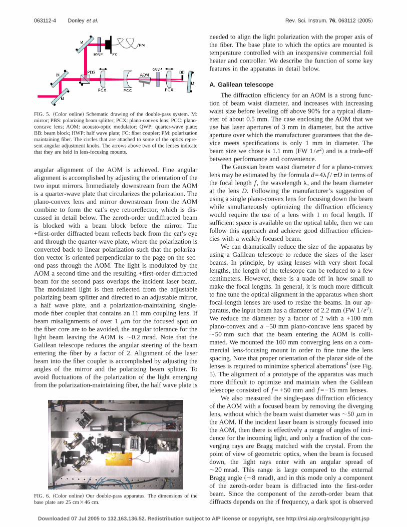
angular alignment of the AOM is achieved. Fine angularalignment is accomplished by adjusting the orientation of thetwo input mirrors. Immediately downstream from the AOMis a quarter-wave plate that circularizes the polarization. Theplano-convex lens and mirror downstream from the AOMcombine to form the cat’s eye retroreflector, which is dis-cussed in detail below. The zeroth-order undiffracted beamis blocked with a beam block before the mirror. The+first-order diffracted beam reflects back from the cat’s eyeand through the quarter-wave plate, where the polarization isconverted back to linear polarization such that the polariza-tion vector is oriented perpendicular to the page on the sec-ond pass through the AOM. The light is modulated by theAOM a second time and the resulting +first-order diffractedbeam for the second pass overlaps the incident laser beam.The modulated light is then reflected from the adjustablepolarizing beam splitter and directed to an adjustable mirror,a half wave plate, and a polarization-maintaining single-mode fiber coupler that contains an 11 mm coupling lens. Ifbeam misalignments of over 1mm for the focused spot onthe fiber core are to be avoided, the angular tolerance for thelight beam leaving the AOM is,0.2 mrad. Note that theGalilean telescope reduces the angular steering of the beamentering the fiber by a factor of 2. Alignment of the laserbeam into the fiber coupler is accomplished by adjusting theangles of the mirror and the polarizing beam splitter. Toavoid fluctuations of the polarization of the light emergingfrom the polarization-maintaining fiber, the half wave plate is
needed to align the light polarization with the proper axis ofthe fiber. The base plate to which the optics are mounted istemperature controlled with an inexpensive commercial foilheater and controller. We describe the function of some keyfeatures in the apparatus in detail below.
A. Galilean telescope
The diffraction efficiency for an AOM is a strong func-tion of beam waist diameter, and increases with increasingwaist size before leveling off above 90% for a typical diam-eter of about 0.5 mm. The case enclosing the AOM that weuse has laser apertures of 3 mm in diameter, but the activeaperture over which the manufacturer guarantees that the de-vice meets specifications is only 1 mm in diameter. Thebeam size we chose is 1.1 mmsFW 1/e2d and is a trade-offbetween performance and convenience.
The Gaussian beam waist diameterd for a plano-convexlens may be estimated by the formulad=4lf /pD in terms ofthe focal lengthf, the wavelengthl, and the beam diameterat the lensD. Following the manufacturer’s suggestion ofusing a single plano-convex lens for focusing down the beamwhile simultaneously optimizing the diffraction efficiencywould require the use of a lens with 1 m focal length. Ifsufficient space is available on the optical table, then we canfollow this approach and achieve good diffraction efficien-cies with a weakly focused beam.
We can dramatically reduce the size of the apparatus byusing a Galilean telescope to reduce the sizes of the laserbeams. In principle, by using lenses with very short focallengths, the length of the telescope can be reduced to a fewcentimeters. However, there is a trade-off in how small tomake the focal lengths. In general, it is much more difficultto fine tune the optical alignment in the apparatus when shortfocal-length lenses are used to resize the beams. In our ap-paratus, the input beam has a diameter of 2.2 mmsFW 1/e2d.We reduce the diameter by a factor of 2 with a +100 mmplano-convex and a −50 mm plano-concave lens spaced by,50 mm such that the beam entering the AOM is colli-mated. We mounted the 100 mm converging lens on a com-mercial lens-focusing mount in order to fine tune the lensspacing. Note that proper orientation of the planar side of thelenses is required to minimize spherical aberrations4 ssee Fig.5d. The alignment of a prototype of the apparatus was muchmore difficult to optimize and maintain when the Galileantelescope consisted off = +50 mm andf =−15 mm lenses.
We also measured the single-pass diffraction efficiencyof the AOM with a focused beam by removing the diverginglens, without which the beam waist diameter was,50 mm inthe AOM. If the incident laser beam is strongly focused intothe AOM, then there is effectively a range of angles of inci-dence for the incoming light, and only a fraction of the con-verging rays are Bragg matched with the crystal. From thepoint of view of geometric optics, when the beam is focuseddown, the light rays enter with an angular spread of,20 mrad. This range is large compared to the externalBragg angles,8 mradd, and in this mode only a componentof the zeroth-order beam is diffracted into the first-orderbeam. Since the component of the zeroth-order beam thatdiffracts depends on the rf frequency, a dark spot is observed
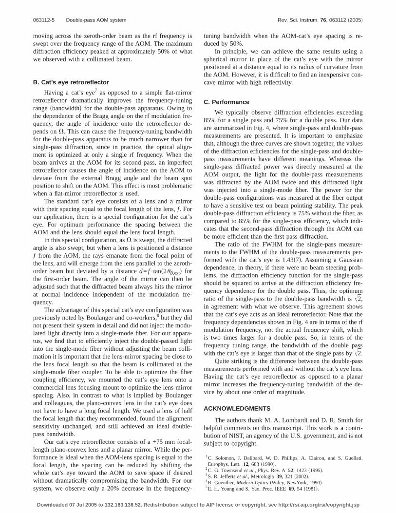
FIG. 6. sColor onlined Our double-pass apparatus. The dimensions of thebase plate are 25 cm346 cm.
FIG. 5. sColor onlined Schematic drawing of the double-pass system. M:mirror; PBS: polarizing beam splitter; PCX: plano-convex lens; PCC: plano-concave lens; AOM: acousto-optic modulator; QWP: quarter-wave plate;BB: beam block; HWP: half wave plate; FC: fiber coupler; PM: polarizationmaintaining fiber. The circles that are attached to some of the optics repre-sent angular adjustment knobs. The arrows above two of the lenses indicatethat they are held in lens-focusing mounts.
063112-4 Donley et al. Rev. Sci. Instrum. 76, 063112 ~2005!
Downloaded 07 Jul 2005 to 132.163.136.52. Redistribution subject to AIP license or copyright, see http://rsi.aip.org/rsi/copyright.jsp
moving across the zeroth-order beam as the rf frequency isswept over the frequency range of the AOM. The maximumdiffraction efficiency peaked at approximately 50% of whatwe observed with a collimated beam.
B. Cat’s eye retroreflector
Having a cat’s eye7 as opposed to a simple flat-mirrorretroreflector dramatically improves the frequency-tuningrangesbandwidthd for the double-pass apparatus. Owing tothe dependence of the Bragg angle on the rf modulation fre-quency, the angle of incidence onto the retroreflector de-pends onV. This can cause the frequency-tuning bandwidthfor the double-pass apparatus to be much narrower than forsingle-pass diffraction, since in practice, the optical align-ment is optimized at only a single rf frequency. When thebeam arrives at the AOM for its second pass, an imperfectretroreflector causes the angle of incidence on the AOM todeviate from the external Bragg angle and the beam spotposition to shift on the AOM. This effect is most problematicwhen a flat-mirror retroreflector is used.
The standard cat’s eye consists of a lens and a mirrorwith their spacing equal to the focal length of the lens,f. Forour application, there is a special configuration for the cat’seye. For optimum performance the spacing between theAOM and the lens should equal the lens focal length.
In this special configuration, asV is swept, the diffractedangle is also swept, but when a lens is positioned a distancef from the AOM, the rays emanate from the focal point ofthe lens, and will emerge from the lens parallel to the zeroth-order beam but deviated by a distanced= f · tans2uB,extd forthe first-order beam. The angle of the mirror can then beadjusted such that the diffracted beam always hits the mirrorat normal incidence independent of the modulation fre-quency.
The advantage of this special cat’s eye configuration waspreviously noted by Boulanger and co-workers,8 but they didnot present their system in detail and did not inject the modu-lated light directly into a single-mode fiber. For our appara-tus, we find that to efficiently inject the double-passed lightinto the single-mode fiber without adjusting the beam colli-mation it is important that the lens-mirror spacing be close tothe lens focal length so that the beam is collimated at thesingle-mode fiber coupler. To be able to optimize the fibercoupling efficiency, we mounted the cat’s eye lens onto acommercial lens focusing mount to optimize the lens-mirrorspacing. Also, in contrast to what is implied by Boulangerand colleagues, the plano-convex lens in the cat’s eye doesnot have to have a long focal length. We used a lens of halfthe focal length that they recommended, found the alignmentsensitivity unchanged, and still achieved an ideal double-pass bandwidth.
Our cat’s eye retroreflector consists of a +75 mm focal-length plano-convex lens and a planar mirror. While the per-formance is ideal when the AOM-lens spacing is equal to thefocal length, the spacing can be reduced by shifting thewhole cat’s eye toward the AOM to save space if desiredwithout dramatically compromising the bandwidth. For oursystem, we observe only a 20% decrease in the frequency-
tuning bandwidth when the AOM-cat’s eye spacing is re-duced by 50%.
In principle, we can achieve the same results using aspherical mirror in place of the cat’s eye with the mirrorpositioned at a distance equal to its radius of curvature fromthe AOM. However, it is difficult to find an inexpensive con-cave mirror with high reflectivity.
C. Performance
We typically observe diffraction efficiencies exceeding85% for a single pass and 75% for a double pass. Our dataare summarized in Fig. 4, where single-pass and double-passmeasurements are presented. It is important to emphasizethat, although the three curves are shown together, the valuesof the diffraction efficiencies for the single-pass and double-pass measurements have different meanings. Whereas thesingle-pass diffracted power was directly measured at theAOM output, the light for the double-pass measurementswas diffracted by the AOM twice and this diffracted lightwas injected into a single-mode fiber. The power for thedouble-pass configurations was measured at the fiber outputto have a sensitive test on beam pointing stability. The peakdouble-pass diffraction efficiency is 75% without the fiber, ascompared to 85% for the single-pass efficiency, which indi-cates that the second-pass diffraction through the AOM canbe more efficient than the first-pass diffraction.
The ratio of the FWHM for the single-pass measure-ments to the FWHM of the double-pass measurements per-formed with the cat’s eye is 1.43s7d. Assuming a Gaussiandependence, in theory, if there were no beam steering prob-lems, the diffraction efficiency function for the single-passshould be squared to arrive at the diffraction efficiency fre-quency dependence for the double pass. Thus, the optimumratio of the single-pass to the double-pass bandwidth isÎ2,in agreement with what we observe. This agreement showsthat the cat’s eye acts as an ideal retroreflector. Note that thefrequency dependencies shown in Fig. 4 are in terms of the rfmodulation frequency, not the actual frequency shift, whichis two times larger for a double pass. So, in terms of thefrequency tuning range, the bandwidth of the double passwith the cat’s eye is larger than that of the single pass byÎ2.
Quite striking is the difference between the double-passmeasurements performed with and without the cat’s eye lens.Having the cat’s eye retroreflector as opposed to a planarmirror increases the frequency-tuning bandwidth of the de-vice by about one order of magnitude.
ACKNOWLEDGMENTS
The authors thank M. A. Lombardi and D. R. Smith forhelpful comments on this manuscript. This work is a contri-bution of NIST, an agency of the U.S. government, and is notsubject to copyright.
1C. Solomon, J. Dalibard, W. D. Phillips, A. Clairon, and S. Guellati,Europhys. Lett.12, 683 s1990d.
2C. G. Townsendet al., Phys. Rev. A52, 1423s1995d.3S. R. Jeffertset al., Metrologia 39, 321 s2002d.4R. Guenther,Modern OpticssWiley, NewYork, 1990d.5E. H. Young and S. Yao, Proc. IEEE69, 54 s1981d.
063112-5 Double-pass AOM system Rev. Sci. Instrum. 76, 063112 ~2005!
Downloaded 07 Jul 2005 to 132.163.136.52. Redistribution subject to AIP license or copyright, see http://rsi.aip.org/rsi/copyright.jsp
6Products or companies named here are cited only in the interest of com-plete scientific description, and neither constitute nor imply endorsementby NIST or by the US government. Other products may be found to servejust as well.
7J. J. Snyder, Appl. Opt.14, 1825s1975d.8J. S. Boulanger, M. C. Gagné, and R. J. Douglas., Proceedings of the 11thEuropean Frequency and Time Forum, Neuchatel, France, 4–6, March,1997, pp. 567–571.
063112-6 Donley et al. Rev. Sci. Instrum. 76, 063112 ~2005!
Downloaded 07 Jul 2005 to 132.163.136.52. Redistribution subject to AIP license or copyright, see http://rsi.aip.org/rsi/copyright.jsp
AA Sa 18, rue Nicolas Appert 91898 ORSAY France Tel : +33 (0)1 76 91 50 12 – Fax : +33 (0)1 76 91 50 31 – www.aaoptoelectronic.com
QUANTA TECH 116 West, 23rd Street - Suite 500 New York, NY 10011 USA Tel: 646 375 2452 - Fax: 866 978 2682 – www.quanta-tech.com
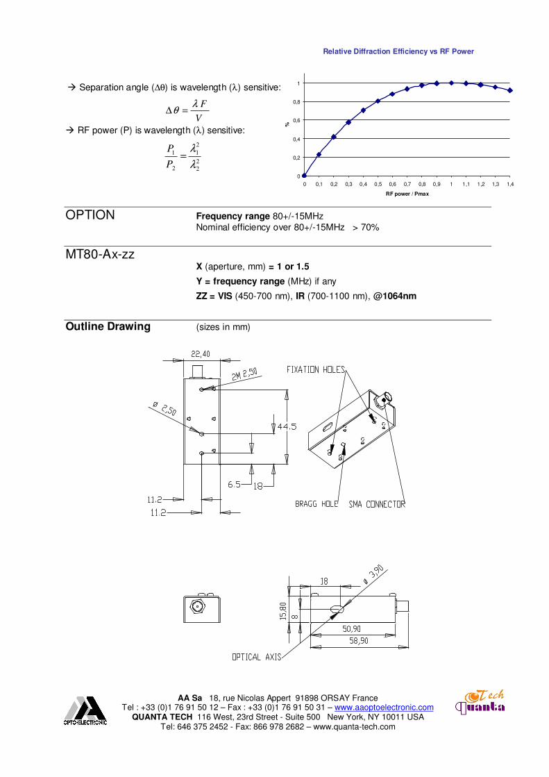
MT80 AO Modulator/Shifter
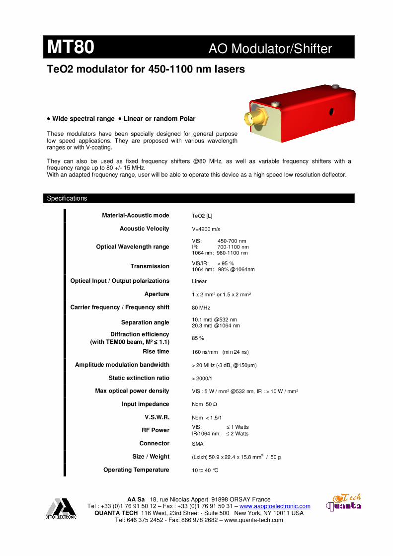
TeO2 modulator for 450-1100 nm lasers
•••• Wide spectral range •••• Linear or random Polar These modulators have been specially designed for general purpose low speed applications. They are proposed with various wavelength ranges or with V-coating. They can also be used as fixed frequency shifters @80 MHz, as well as variable frequency shifters with a frequency range up to 80 +/- 15 MHz. With an adapted frequency range, user will be able to operate this device as a high speed low resolution deflector.
AA Sa 18, rue Nicolas Appert 91898 ORSAY France Tel : +33 (0)1 76 91 50 12 – Fax : +33 (0)1 76 91 50 31 – www.aaoptoelectronic.com
QUANTA TECH 116 West, 23rd Street - Suite 500 New York, NY 10011 USA Tel: 646 375 2452 - Fax: 866 978 2682 – www.quanta-tech.com
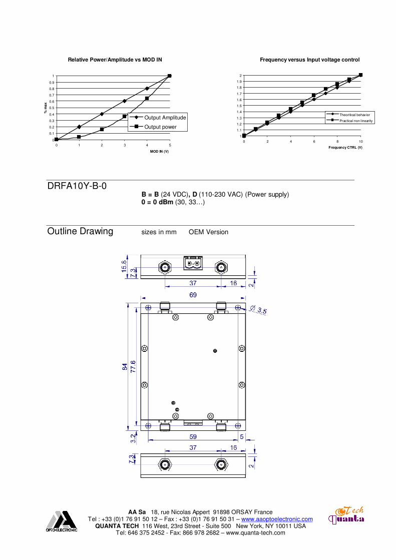
DRFA10Y Fast VCO driver
Fast sweeping time VCO
•••• Random access or raster scan •••• OEM & Laboratory versions •••• Sweeping time ≤≤≤≤ 1 µs
These Voltage Controlled Oscillators are the simplest way to control a deflector or a variable frequency shifter, in random access or raster scan mode. A voltage between 0 and 10 V is applied on the frequency control input in order to sweep the frequency. The sweeping time from Fmin to Fmax can be as low as 1 µs. The typical stability of a VCO is 50 to 100 KHz/°C : in option higher stabilities are proposed, and for the sharpest applications, a DDS will be preferred. These drivers are used in combination with AA amplifiers.
Specifications
Frequency range Up to one octave (40-100, 60-150, 80-200, 140-300, 190-350)
Matched to AO device at factory
Frequency stability Nom +/- 50 to 100kHz/°C
Sweeping time ≤ 1 µs
Frequency control 1 Analog 0-10 V / 1 KΩ
Linearity (full bandwidth) Nom +/- 5 %
Rise time / Fall time (10-90 %) < 10 ns
Modulation input control 1 Video In Analog 0-5 V / 50 Ω
Extinction ratio 2 > 40 dB
Harmonics Nom > 20 dBc
Output RF power 3 Nom - 30 to 0 dBm (to be associated with AA Amplifier)
Output impedance 50 Ω
V.S.W.R. ≤ 1.5 : 1
Power supply OEM version : 24 VDC – nom 150 mA
Laboratory version 4 : 110-230 VAC – 50-60 Hz
Input / Output connectors 2 SMA
Size OEM version : 84 x 69 x 15.8 mm
3
Laboratory version 4 : 310 x 250 x 105 mm
3
Weight OEM version : 0.2 Kg
Laboratory version 4 : 4 Kg
Cooling Conduction through baseplate
Maximimun case temperature 50 °C
Operating temperature 10 to 40 °C
1 On request different Video In are proposed : 0-5 V/50 Ohms, 0-5V/500 Ohms, TTL…
2 Other values or models on request
3 Fully adjustable with screw potentiometer from 0 to 1 watt or 0 to 2 Watts
4 These versions are complete turn key systems with minimum set up time.
The source and convenient amplifiers are integrated in a rack which is supplied with 110-230 VAC. A selection switch on front panel allows the user to select both operating modes:
- CW mode: internal CW modulation of RF power with front pannel cursor. - AM mode: external amplitude modulation controlled through external modulation input. - F CW mode: internal CW modulation of RF Frequency with front pannel cursor. - FM mode: external frequency modulation controlled through external input.
AA Sa 18, rue Nicolas Appert 91898 ORSAY France Tel : +33 (0)1 76 91 50 12 – Fax : +33 (0)1 76 91 50 31 – www.aaoptoelectronic.com
QUANTA TECH 116 West, 23rd Street - Suite 500 New York, NY 10011 USA Tel: 646 375 2452 - Fax: 866 978 2682 – www.quanta-tech.com
DRFA10Y-B-0 B = B (24 VDC), D (110-230 VAC) (Power supply) 0 = 0 dBm (30, 33…)
Outline Drawing sizes in mm OEM Version
Relative Power/Amplitude vs MOD IN
0
0.1
0.2
0.3
0.4
0.5
0.6
0.7
0.8
0.9
1
0 1 2 3 4 5
MOD IN (V)
% m
ax
Output Amplitude
Output power
Frequency versus Input voltage control
1
1.1
1.2
1.3
1.4
1.5
1.6
1.7
1.8
1.9
2
0 2 4 6 8 10
Frequency CTRL (V)
Theoritical behavior
Practical non linearity
AA Sa 18, rue Nicolas Appert 91898 ORSAY France Tel : +33 (0)1 76 91 50 12 – Fax : +33 (0)1 76 91 50 31 – www.aaoptoelectronic.com
QUANTA TECH 116 West, 23rd Street - Suite 500 New York, NY 10011 USA Tel: 646 375 2452 - Fax: 866 978 2682 – www.quanta-tech.com
AMPA–B-30 -33 Large Band RF amplifier
RF amplifiers 1 & 2 Watts
•••• Large band •••• General purposes
These amplifiers are made for general purpose applications, covering frequency ranges up to 450-600 MHz. In association with a VCO driver or a DDS driver, they will provide the necessary RF power to drive an acousto-optic device up to 2 watts.
Specifications
Frequency range1
1 Watt : 20-450 MHz 2 watts : 20-600 MHz
Gain2
1 Watt : ≥ 33 dB
2 watts : ≥ 40 dB
Gain Flatness
Nom +/- 0.5 dB, ≤ +/1 dB
Noise Figure
1 Watt : nom 5 dB 2 watts : nom 7 dB
Output RF Power (1 dB compression)
≥ 30 dBm (≥ 29.5 dBm @ <40 MHz), 1 Watt
≥ 33 dBm , 2 Watts
Output Impedance
50 Ω
CLASS
A
Power supply3
1 Watt : 24 +/- 0.5 VDC - ≤ 340 mA
2 watts : 24 +/- 0.5 VDC - ≤ 500 mA
Input / Output connectors
SMA female
Size
76 x 40 x 42 mm3
Weight
0.22 Kg
Heat exchange
Conduction through baseplate
Operating temperature
-10 to +55 °C
1 Optimized at factory according to AO device if any
2 Other values or models on request
3 110/230 VAC available on request
AA Sa 18, rue Nicolas Appert 91898 ORSAY France Tel : +33 (0)1 76 91 50 12 – Fax : +33 (0)1 76 91 50 31 – www.aaoptoelectronic.com
QUANTA TECH 116 West, 23rd Street - Suite 500 New York, NY 10011 USA Tel: 646 375 2452 - Fax: 866 978 2682 – www.quanta-tech.com
Intended useThe card camera with manual focus adjustment is designed for surveillance and security purposes in uncontrolled and critical areas (such as shop, door intercoms, entrance areas or parking lots etc.). The recorded images can be played back with sound on any suitable display device with video input (such as TV or monitor).The card camera is not permitted to use without protection (without the corresponding casing). It must be power by 12 V= only. Contact with moisture must be avoided at all times.Any usage other than described above is not permitted and can damage the product and lead to associated risks such as short-circuit, fire, electric shock, etc. No part of the product may be modified or rebuilt. Please read the operating instructions thoroughly and keep the operating instructions for further reference.
Safety instructionsWe do not resume liability for resulting damages to property or personal injury if the product has been abused in any way or damaged by improper use or failure to observe these operating instructions. The guarantee will then expire!An exclamation mark in a triangle indicates important information in the operating instructions. Carefully read the whole operating instructions before operating the device, otherwise there is risk of danger.
Unauthorised conversion and/or modification of the device are inadmissible because of safety and approval reasons (CE).The card camera must not be exposed to dust, extreme temperatures, direct sunlight, intense vibration or dampness.The card camera must be installed in proper housing in prior to operation.The card camera should not be installed in vicinity of strong magnetic or electric fields, e.g. mobile phones, walkie-talkies, electric motors etc.The card camera is only permitted to be powered by power pack or a battery/accumulator with screened and stabilized direct voltage. The voltage source must be able to supply sufficient power.After rapid temperature changes, the device needs approximately 15 minutes of stabilization to accommodate to the new ambient temperature before use.When connecting the camera, make sure that the connection cables are not damaged by sharp edges.When using other devices or tools to assist the installation, the corresponding operating instructions must be observed.When using a power pack as the voltage source, valid safety regulations must be followed under all circumstances. Car chargers and toy transformers are not suitable as voltage sources and will lead to damage to the components or to the device failing to function.In commercial institutions, the accident prevention regulations of the relevant professional insurance association for electrical systems and operating materials have to be observed.If safe operation of the card camera is no longer possible, disconnect the appliance immediately and secure it against inadvertent operation. Safe operation is no longer possible if:
the device shows visible damages,the device no longer works andthe device was stored under unfavourable conditions for a long period of time,the device was subject to considerable transport stress.
If you have any doubt about the card camera installation or operation, consult adequate qualified personnel.Packaging materials must not be lying around carelessly. They could become dangerous toys in hands of children.This card camera is not a toy and should be kept out of reach of children!Servicing, adjustment or repair works must only be carried out by a specialist/ specialist workshop.If any questions arise that are not answered in this operating instruction, please contact our Technical Advisory Service or other experts.
Connection and operationUse 12V= voltage source to power the card camera. Never try to operate the camera with another voltage source. The DC source for the camera has to supply a current of 100 mA as minium load capacity. Never overload the voltage source.If you use a power pack as voltage source, this must be turned off during connecting.Observe the polarity when connecting the voltage supply. If the polarity is not correct, the components of the card camera may be destroyed.
Camera connectionsConnect the small white plug of the connection cable with the camera module. This only fits into the socketwith the right polarity.
Video connectionConnect the video input of your TV or monitor with the yellow cinch socket of the cameramodule.
Use a suitable optional cinch connection cable (polarity: inside video, outside ground).For any extensions, only use suitably shielded cinch cables. The use of other, unsuitable cables may lead to interference.Keep the length of the cable as short as possible.
Power supply connectionConnect the red power supply plug of the camera connection cable (VDC) with a matching power pack. The DC low voltage plug must have the following properties:
Dimensions outside 5.5 mm, inner hole 2.1 mm.Polarity inside plus (+), outside minus (-).
Manual focal distance adjustmentLoosen the screw on the len mount.Turn the len clockwise/ anticlockwise to adjust the focal distance.Tighten the screw after the desired focal distance is set.
•
•
••
•
•
••
•
•
•
----
•
•
•••
--
1.2.3.
Version 06/06Version 06/06
Maintenance and cleaningApart from sporadically cleaning the lens, the card camera is maintenance-free.Use a clean, lint-free, antistatic and dry cloth to clean the len. Do not use any abrasive or chemical agents or detergents containing solvents.
DisposalIn order to preserve, protect and improve the quality of environment, protect human health and utilise natural resources prudently and rationally, the user should return unserviceable product to relevant facilities in accordance with statutory regulations.The crossed-out wheeled bin indicates the product needs to be disposed separately and not as municipal waste.
Technical dataItem no. 190974 190988
Operating voltage 12V= 12V=
Current consumption approx. 100mA approx. 100mA
Image sensor 1/3” CCD black/white 1/3” CCD colour
Video format PAL PAL
Lens (focal distance) 1.5m 1.5m
Video level 1.0Vp-p ± 0.2 1.0Vp-p ± 0.2
Light intensity 0.01 Lux at F1.2 0.5 Lux at F1.2
Shutter speed 1/50 ~ 1/100000 second 1/50 ~ 1/100000 second
Effective pixels PAL: 512 x 582 PAL: 512 x 582
Resolution (TV lines) 380 420
Video signal-to-noise ratio > 48dB > 48dB
Operating temperature -20ºC to +55ºC -20ºC to +55ºC
Bestimmungsgemäße VerwendungDas Kameramodul mit manueller Fokusanpassung ist für Überwachungs- und Sicherheitszwecke in wichtigen, unbeaufsichtigten Bereichen (z. B. Geschäftsräumen, Gegensprechanlagen, Einfahrten und Parkgaragen konzipiert. Die Aufnahmen können auf beliebigen Wiedergabegeräten mit Videoeingang, wie etwa einem TV oder Monitor, wiedergegeben werden.Das Kameramodul darf nicht ohne Schutzgehäuse eingesetzt werden und kann ausschließlich mit 12 V DC betrieben werden. Kontakt mit Feuchtigkeit muss unbedingt vermieden werden!Das Kameramodul anderweitig als oben beschrieben einzusetzen, ist nicht zulässig und führt zu einer Beschädigung des Produkts. Damit verbundene Risiken beinhalten Kurzschluss, Brandgefahr, Elektroschock, usw. Weder das Produkt noch Teile davon dürfen geändert oder nachgebaut werden. Lesen Sie die Bedienungsanweisung aufmerksam durch, und bewahren Sie sorgfältig auf.
SicherheitshinweiseBei Schäden, die durch Nichtbeachtung dieser Bedienungsanleitung verursacht werden, erlischt der Garantieanspruch! Für Folgeschäden und bei Sach- und Personenschäden, die durch unsachgemäße Handhabung oder Nichtbeachten der Sicherheitshinweise verursacht werden, übernehmen wir keine Haftung!Ein Ausrufezeichen im Dreieck weist auf wichtige Informationen in der Bedienungsanleitung hin. Lesen Sie die gesamte Bedienungsanleitung durch und beachten Sie unbedingt alle Sicherheitsanweisungen.
Das Produkt darf nicht verändert oder umgebaut werden, sonst erlischt nicht nur die Zulassung (CE), sondern auch die Garantie/Gewährleistung.Das Produkt darf nicht extremen Temperaturen, direktem Sonnenlicht, intensiver Vibration, Staub oder Feuchtigkeit ausgesetzt werden.Das Kameramodul muss vor der Inbetriebnahme in ein geeignetes Gehäuse installiert werden.Die Installation der Sensorkamera in der Nähe starker Magnet- oder Elektrofelder, wie etwa Mobiltelefone, Funkgeräte, Elektromotoren, usw. ist nicht empfehlenswert.Das Kameramodul kann nur mit einem Netzteil oder einem Akku mit stabilisierter Gleichspannung betrieben werden. Der Strom der Spannungsquelle muss ausreichend sein.Nach extremen Temperaturunterschieden benötigt das Gerät 15 Minuten zur Stabilisierung, um sich an die neue Umgebungstemperatur anzupassen, bevor es in Betrieb genommen werden kann.Beim Anschließen der Kamera ist sicherzustellen, dass die Verbindungskabel nicht durch scharfe Kanten beschädigt werden.Beim Einsatz anderer Geräte oder Werkzeuge müssen die jeweiligen Bedienungsanweisungen beachtet werden.Beim Einsatz eines Netzteils als Spannungsquelle müssen die geltenden Sicherheitsrichtlinien auf alle Fälle befolgt werden. Autoladegeräte und Netzteile für Kinderspielzeug sind nicht als Spannungsquellen geeignet und führen dazu, dass die Komponenten beschädigt werden oder das Gerät nicht funktioniert.In gewerblichen Einrichtungen sind die Unfallverhütungsvorschriften des Verbandes der gewerblichen Berufsgenossenschaften für elektrische Anlagen und Betriebsmittel zu beachten.Wenn anzunehmen ist, dass ein gefahrloser Betrieb nicht mehr möglich ist, so ist das Gerät außer Betrieb zu setzen und gegen unbeabsichtigten Betrieb zu sichern. Es ist anzunehmen, dass ein gefahrloser Betrieb nicht mehr möglich ist, wenn:
das Gerät sichtbare Beschädigungen aufweist,das Gerät nicht mehr arbeitet undnach längerer Lagerung unter ungünstigen Verhältnissen odernach schweren Transportbeanspruchungen.
Falls Sie bezüglich Installation oder Betrieb des Kameramoduls Zweifel haben, wenden Sie sich bitte an ausreichend qualifiziertes Personal.Lassen Sie niemals Verpackungsmaterial unachtsam herumliegen. Plastikfolien/Taschen usw. können für Kinder zu einem gefährlichen Spielzeug werden, es besteht Erstickungsgefahr.Das Produkt ist kein Spielzeug und muss außerhalb der Reichweite von Kindern gehalten werden!Wartung, Anpassungs- und Reparaturarbeiten dürfen nur von einer Fachkraft bzw. einer Fachwerkstatt durchgeführt werden.Sollten Sie noch Fragen haben, die in dieser Bedienungsanleitung nicht beantwortet werden, so wenden Sie sich bitte an unseren technischen Kundendienst oder andere Fachleute.
Anschluss und BetriebZum Betrieb der Sensorkamera ist eine 12 V-Spannungsquelle zu verwenden. Unter keinen Umständen ist eine andere Spannungsquelle zu verwenden. Die Spannungsquelle muss einen Ausgangsstrom von 100 mA liefern können. Ein überlasten der Spannungsquelle ist unbedingt zu vermeiden.Wenn Sie ein Netzteil als Spannungsquelle verwenden, muss dieses beim Anschließen ausgeschaltet sein.Beim Anschließen ist die Polarität zu beachten. Unterlassen Sie dies, können die Komponenten der Sensorkamera beschädigt werden.
An dem Kabel ist eine gelbe Cinch Buchse montiert, für den direkten Anschluss an einem TV Gerät oder Monitor FBAS ( CEs ist auch eine DC Buchse ( rot ) montiertAbmessungen aussen Ø 5,5 mm innen Ø 2,1 mmPolarität innen Plus ( +) aussen Minus ( - )
Manuelles Anpassen der Brennweite möglichLockern Sie die Schraube am Linsenansatz.Drehen Sie die Linse im Uhrzeigersinn/gegen den Uhrzeigersinn, um die Brennweite anzupassen.Ziehen Sie nach dem Einstellen der gewünschten Brennweite die Schraube nach.
•
•
••
•
•
•
•
•
•
•
----
•
•
••
•
1.2.3.
Version 06/06Version 06/06
Wartung und ReinigungAußer dem gelegentlichen Reinigen der Linse muss das Kameramodul nicht gewartet werden.Verwenden Sie ein sauberes, flusenfreies, antistatisches, trockenes Tuch zum Reinigen der Linse. Verwenden Sie keine Glanz- oder chemischen Mittel bzw. Lösungsmittel.
EntsorgungIm Interesse unserer Umwelt und um die verwendeten Rohstoffe möglichst vollständig zu recyceln, ist der Verbraucher aufgefordert, gebrauchte und defekte Geräte zu den öffentlichen Sammelstellen für Elektroschrott zu bringen.Das Zeichen der durchgestrichenen Mülltonne mit Rädern bedeutet, dass dieses Produkt an einer Sammelstelle für Elektronikschrott abgegeben werden muß, um es durch Recycling einer bestmöglichen Rohstoffwiederverwertung zuzuführen.
Technische DatenBest.-Nr. 190974 190988
Betriebsspannung 12V= 12V=
Stromaufnahme ca. 100 mA ca. 100 mA
Bildsensor 1/3” CCD Schwarz/weiß 1/3” CCD Farbe
Videoformat PAL PAL
Linse (Brennweite) 1,5m 1,5m
Videopegel 1,0Vp-p ± 0.2 1,0Vp-p ± 0.2
Lichtempfindlichkeit 0,01 Lux bei F1.2 0,5 Lux bei F1.2
Diese Bedienungsanleitung ist eine Publikation der Conrad Electronic GmbH, Klaus-Conrad-Straße 1, D-92240 Hirschau.Diese Bedienungsanleitung entspricht dem technischen Stand bei Drucklegung. Änderung in Technik und Änderungen vorbehalten.
These operating instructions are published by Conrad Electronic GmbH, Klaus-Conrad-Straße 1, D-92240 Hirschau/GermanyThe operating instructions reflect the current technical specifications at time of print. We reserve the right to change the technical or physical specifications.
Caméra de surveillance DTCN° de commande 19 09 74 1/3” Noir/blancN° de commande 19 09 88 1/3” Couleur
Utilisation prévueLa caméra à carte à réglage manuel de la mise au point a été conçue pour la surveillance et la sécurité dans les zones non contrôlées et critiques (par ex. magasins, interphones, entrées, parkings, etc.). Les images enregistrées peuvent être visionnées avec le son sur tout écran adéquat et disposant d’une entrée vidéo (tel que télévision ou moniteur).Il est interdit d’utiliser la caméra à carte sans protection (sans le boîtier approprié). Elle ne doit être alimentée que par 12 V=. Il est essentiel d’éviter tout contact avec l’humidité.Toute utilisation autre que celle stipulée ci-dessus n’est pas permise et peut endommager ce produit et présenter des risques de courts-circuits, d’incendie, de chocs électriques, etc. Il n’est permis ni de modifier le produit ni de transformer aucun élément de cet appareil. Veuillez bien lire ce mode d’emploi et le garder à titre de référence. Veuillez bien lire toutes les instructions avant d’utiliser cet appareil afin d’écarter tout danger.
Consignes de sécuritéNous déclinons toute responsabilité pour d’éventuels dommages matériels ou corporels dus à un emploi abusif, un maniement incorrect ou à la non observation des consignes de sécurité. De tels cas entraîneront l’annulation de la garantie !Un point d’exclamation dans un triangle indique des informations importantes dans ce mode d’emploi qui doivent être strictement respectées.
Pour des raisons de sécurité et d’approbation (CE), il est interdit de modifier la construction et/ou de modifier l’appareil.Ne pas exposer la caméra à carte à la poussière, aux extrêmes de température, à la lumière directe du soleil, aux fortes vibrations ou à l’humidité.Installer impérativement la caméra à carte dans le boîtier approprié avant de l’utiliser.Ne pas utiliser la caméra à carte à proximité de champs magnétiques ou électriques forts, par ex. téléphones portables, walkies-talkies, moteurs électriques, etc.La caméra à carte ne peut être alimentée que par des blocs d’alimentation ou une pile/un accumulateur disposant de tension directe protégée et stabilisée. La source de tension doit pouvoir fournir la puissance requise.Après de rapides changements de température, il faut environ 15 minutes pour permettre à l’appareil de se stabiliser et de s’accoutumer à la nouvelle température ambiante avant emploi.Au moment de connecter la caméra, s’assurer que les câbles de connexion n’ont pas été endommagés par des arêtes vives.Si vous vous servez d’autres appareils ou outils pour installer l’appareil, il convient de respecter les instructions correspondantes.Si vous utilisez un bloc d’alimentation comme source de tension, il convient de respecter les consignes de sécurité appropriées en toute circonstance. Les batteries automobiles et les transformateurs pour jouets ne peuvent être utilisés comme source de tension ; elles endommageront les composantes ou l’appareil et empêcheront son bon fonctionnement.Dans les établissements commerciaux, il convient d’observer les consignes de prévention des accidents appropriées à l’assurance de l’association professionnelle pour les systèmes électriques et les matériaux de fonctionnement.S’il n’est plus possible d’utiliser la caméra à carte en toute sécurité, il faut immédiatement débrancher l’appareil et le sécuriser contre tout usage involontaire. Un fonctionnement sûr n’est plus possible si :
L’appareil présente des signes d’endommagement,L’appareil ne fonctionne plus etL’appareil a été stocké dans des conditions défavorables pendant une période prolongée,L’appareil a été soumis à une contrainte de transport considérable.
Si vous avez un doute quelconque concernant l’installation ou l’utilisation de la caméra à carte, veuillez consulter le personnel qualifié approprié.Ne pas laisser traîner les emballages car ils pourraient poser des dangers aux enfants.Cette caméra à carte n’est pas un jouet et doit être gardée hors de portée des enfants !Tout entretien, ajustement ou réparation ne doit être effectué que par un spécialiste/atelier spécialisé.Si vous avez des questions auxquelles le mode d’emploi n’a pas pu répondre, consultez notre service de renseignements techniques ou un spécialiste.
Raccordement et utilisationUtiliser une source de tension de 12V= pour alimenter la caméra à carte. Ne jamais essayer de faire fonctionner la caméra avec une autre source de tension. La source de courant direct pour la caméra doit fournir un courant de 100 mA de capacité de charge minimum. Ne jamais surcharger la source de tension.Si vous utilisez un bloc d’alimentation comme source de tension, il faut éteindre ce dernier au moment du raccordement.Respecter la polarité au moment du raccordement de la source de tension. Une polarité incorrecte peut détruire les composantes de la caméra à carte.
Installer la caméra à carte dans le boîtier approprié.Connecter le pôle positif de l’entrée vidéo de votre poste de télévision ou moniteur au câble jaune du module de la caméra.Connecter le pôle négatif de l’entrée vidéo de votre poste de télévision ou moniteur au câble noir du module de la caméra.Connecter le pôle négatif de la source de tension au câble de connexion noir du module de la caméra.Connecter le pôle positif de la source de tension au câble de connexion rouge du module de la caméra.Enlever la couverture de protection de la caméra à carte.
Le câble blanc n’est pas utilisé pour ces modèles.
Réglage manuel de la distance focaleDesserrer la vis de la monture de l’objectif.Tourner l’objectif dans le sens des aiguilles d’une montre/ dans le sens contraire des aiguilles d’une montre pour régler la distance focale.Lorsque la distance focale souhaitée est réglée, resserrer la vis.
•
•
••
•
•
•
•
•
•
•
----
•
••••
1.2.
3.
4.5.6.
1.2.
3.
Version 06/06Version 06/06
Entretien et nettoyageLa caméra à carte ne nécessite aucun entretien en dehors d’un nettoyage sporadique de l’objectif.Utiliser un chiffon propre, sec, sans peluche et antistatique pour nettoyer l’objectif. Ne pas se servir de produits chimiques ou abrasifs ou de détergents contenant des solvants.
DispositionAfin de préserver, protéger et améliorer la qualité de l’environnement, protéger la santé humaine et utiliser les ressources naturelles avec prudence et de manière rationnelle, l’utilisateur doit renvoyer tout produit ne pouvant pas subir d’entretien à l‘établissement pertinent conformément à la réglementation statutaire.Le symbole de la poubelle barrée indique que le produit doit être mis au rebut séparément et non en tant que déchet municipal.
Charactéristiques techniquesN° de commande 190974 190988
Tension de fonctionnement 12V= 12V=
Consommation en électricité environ 100mA environ 100mA
Beoogd gebruikDe camerakaart met handmatige brandpuntinstelling is ontworpen voor toezicht en beveiligingsdoeleinden in ongecontroleerde en kritische gebieden (zoals winkels, deurintercomsystemen, toegangssystemen of parkeergarages en dergelijke). De opgeslagen beelden kunnen worden afgespeeld met geluid via elk daarvoor geschikt weergeefapparaat met een video-ingang (zoals een TV of monitor).Het is niet toegestaan om de camerakaart zonder bescherming te gebruiken (zonder de bijbehorende behuizing). De camerakaart mag uitsluitend worden gevoed door een gelijkspanning van 12 V. Contact met vocht dient onder alle omstandigheden te worden voorkomen.Elk ander gebruik dan hierboven beschreven is niet toegestaan en kan tot beschadiging van het apparaat leiden. Bovendien kan dit leiden tot gevaarlijke situaties, zoals kortsluiting, brand, elektrische schokken en dergelijke. Het apparaat mag niet worden veranderd of omgebouwd. Lees daarom deze gebruiksaanwijzing zorgvuldig door en bewaar deze.
VeiligheidsvoorschriftWij aanvaarden geen aansprakelijkheid voor beschadiging van eigendommen of lichamelijk letsel indien het product is misbruikt of is beschadigd door onjuist gebruik of het niet opvolgen van deze gebruiksaanwijzing. In dergelijke gevallen vervalt de garantie! Het uitroepteken in de driehoek wijst op belangrijke passages in deze gebruiksaanwijzing die strikt moeten worden opgevolgd.
In verband met veiligheid en normering (CE) zijn geen aanpassingen en/of wijzigingen aan de camerakaart toegestaan.De camerakaart mag niet worden blootgesteld aan stof, extreme temperaturen, rechtstreeks zonlicht, sterke trillingen of vocht.Voor gebruik dient de camerakaart te worden ingebouwd in een geschikte behuizing.De camerakaart dient niet te worden geïnstalleerd in de nabijheid van sterke magnetische of elektrische velden, bijvoorbeeld mobiele telefoons, walkie-talkies, elektrische motoren en degelijke.De camerakaart mag uitsluitend worden gevoed door een netspanningsadapter of een batterij/accu met een gefilterde en gestabiliseerde gelijkspanning. De voedingsbron dient voldoende vermogen te kunnen leveren.Na snelle temperatuurveranderingen heeft de camerakaart circa 15 minuten nodig om zich te stabiliseren en zich aan te passen aan de nieuwe omgevingstemperatuur voordat deze mag worden gebruikt.Zorg er bij het aansluiten van de camera voor dat de verbindingskabels niet worden beschadigd door scherpe hoeken.Wanneer bij het installeren andere apparaten of hulpmiddelen worden gebruikt, dienen de bijbehorende gebruiksaanwijzingen te worden geraadpleegd.Wanneer een netspanningsadapter als spanningsbron wordt toegepast, dienen onder alle omstandigheden de geldende veiligheidsvoorschriften in acht te worden genomen. Acculaders van auto’s en speelgoedtransformatoren zijn niet geschikt als voedingsbron en kunnen leiden tot beschadiging van de componenten of tot het niet werken van de camera.Indien de camera bedrijfsmatig wordt toegepast, dienen de richtlijnen van de aansprakelijkheidsverzekering van de werkgever met betrekking tot ongevallenpreventie ten aanzien van elektrische apparatuur en relevante bedrijfsmiddelen in acht te worden genomen.Wanneer veilig gebruik van de kamerakaart niet langer mogelijk is, onderbreek dan meteen de voeding en voorkom dat deze zomaar opnieuw kan worden ingeschakeld. Veilig werken is niet meer mogelijk wanneer:
het apparaat zichtbare beschadigingen vertoont,het apparaat niet meer werkt,het apparaat gedurende langere tijd onder ongunstige omgevingscondities is opgeslagen,het apparaat tijdens transport mechanisch is beschadigd.
Neem bij twijfel over het installeren of de werking van de camerakaart contact op met een specialist.Laat verpakkingsmateriaal niet zomaar rondslingeren. Het kan gevaarlijk speelgoed in de handen van kinderen zijn.Deze camerakaart is geen speelgoed en moet buiten het bereik van kinderen worden gehouden!Onderhoud, afstellingen of reparaties mogen uitsluitend worden uitgevoerd door een vakman of een gespecialiseerde onderhoudsdienst.Voor vragen waarop deze gebruiksaanwijzing geen antwoord biedt, kunt u contact opnemen met onze technische dienst of andere specialisten.
Aansluiten en inbedrijfnameGebruik een 12 V gelijkspanningsbron om de camerakaart te voeden. Probeer nooit om de camera met een andere spanning te voeden. De gelijkspanningsvoeding dient een stroom van tenminste 100 mA te kunnen leveren. Let er op dat de voeding nooit overbelast raakt.Wanneer een netspanningsadapter als voedingsbron wordt toegepast, schakel deze dan uit tijdens het aansluiten.Let op de juiste polariteit bij het aansluiten van de voedingsbron. Bij een verkeerde polariteit kunnen de componenten van de camerakaart worden beschadigd.
Monteer de camerakaart in een geschikte behuizing.Verbind de positieve pool van de video-ingang van TV of monitor met de gele draad van de cameramodule.Verbind de negatieve pool van de video-ingang van TV of monitor met de zwarte draad van de cameramodule.Verbind de positieve pool van de voedingsbron met de rode verbindingsdraad van de cameramodule.Verbind de negatieve pool van de voedingsbron met de zwarte verbindingsdraad van de cameramodule.Verwijder de beschermfolie van de camerakaart.
De witte draad wordt niet gebruikt bij deze modellen.
De brandpuntafstand kan handmatig worden ingesteldDraai de schroef van de lensvatting los.Verdraai de lens links of rechtsom voor het afregelen van de brandpuntafstand.Draai de schroef weer vast nadat de gewenste brandpuntafstand is ingesteld.
•
•
••
•
•
•
•
•
•
•
----
••
••
•
1.2.
3.
4.5.6.
1.2.3.
Version 06/06Version 06/06
Onderhoud en reinigingLos van het periodiek reinigen van de lens is de camerakaart onderhoudsvrij.Gebruik een schone, pluisvrije, antistatische en droge doek voor het reinigen van de lens. Gebruik geen agressieve of chemische oplosmiddelen of afwasmiddelen die oplosmiddelen bevatten.
VerwijderingIn het belang van het behoud, de bescherming en de verbetering van de kwaliteit van het milieu, de bescherming van de gezondheid van de mens en een behoedzaam en rationeel gebruik van natuurlijke hulpbronnen dient de gebruiker een niet te repareren of afgedankt product in te leveren bij de desbetreffende inzamelpunten overeenkomstig de wettelijke voorschriften.Het symbool met de doorgekruiste afvalbak geeft aan dat dit product gescheiden van het gewone huishoudelijke afval moet worden ingeleverd.
Technische gegevensBestnr. 190974 190988
Werkspanning 12V= 12V=
Stroomopname circa 100 mA circa 100 mA
Beeldsensor 1/3” CCD zwart/wit 1/3” CCD kleur
Videoformaat PAL PAL
Lens (brandpuntafstand) 1,5m 1,5m
Videoniveau 1,0Vp-p ± 0.2 1,0Vp-p ± 0.2
Lichtgevoeligheid 0,01 lux bij F1.2 0,5 lux bij F1.2
Sluitersnelheid 1/50 tot 1/100.000 seconde 1/50 tot 1/100.000 seconde
Effectieve beeldpunten 512 x 582 512 x 582
Resolutie (TV-lijnen) 380 420
Video signaal/ruis-verhouding > 48dB > 48dB (AGC off)
Deze gebruiksaanwijzing is een publicatie van Conrad Electronic GmbH, Klaus-Conrad-Straße 1, D-92240 Hirschau/Duitsland.Deze werkende instruties voldoet aan de technische eisen bij het ter perse gaan. Wijzigingen in techniek en uitrusting voorbehouden.
Cette notice est une publication de la société Conrad Electronic GmbH, Klaus-Conrad-Straße 1, D-92240 Hirschau/Allemagne.Cette notice est conforme à la règlementation en vigueur lors de l´impression. Données techniques et conditionnement soumis à modifications sans aucun préalable.
1 Taste „Graph“-Modus 8 Signalform-Wahltasten 2 Ein-/Aus-Schalter 9 „Trigger“-Taste (nur für „Sweep“ und „Burst“) 3 „Modulation“-/„Sweep“-/„Burst“-Tasten 10 Taste zum Aktivieren/Deaktivieren von „Output“ 4 Taste zum Abspeichern/ 11 Drehknopf
Zurückrufen von Gerätezuständen 12 Pfeiltasten5 Taste „Utility“-Menü 13 „Sync“-Anschluss6 Taste „Help“-Menü 14 „Output“-Anschluss7 Softkeys zur Menünavigation
Leuchtende Tasten weisen auf aktive Tasten und Funktionen hin ( in obiger Abbildung).
Halten Sie eine Funktionstaste oder einen Softkey gedückt, um die Hilfe für diese Taste oder Funktion aufzurufen. Halten Sie z. B. diese Taste gedrückt: Oder drücken Sie zur Anzeige des Hilfemenüs auf:
Hilfe zu den Tasten
Überblick über die Frontplatte
Die wichtigsten Funktionen der Frontplatte Stellen Sie den Tragegriff ein.
Fassen Sie den Griff an beiden Seiten und ziehen Sie ihn heraus:
Fixieren Sie dann den Griff in der gewünschten Position:
Schließen Sie ein BNC-Kabel am „Output“- Anschluss an. Verbinden Sie dieses anschließend mit Ihrem Testsystem oder Oszilloskop:
Für Schritt 2 bitte
umblättern
Die Grundlagen in acht einfachen Schritten!
1. Leuchtende Tasten weisen darauf hin, dass diese Taste bzw. Funktion derzeit aktiv ist (z. B. die Signalform ). Die meisten Tasten können aktiviert (Taste leuchtet) oder deaktiviert werden.
2. Es wird erst dann ein Signal ausgegeben, wenn die Taste leuchtet.
3. Drücken Sie zur Wahl der Funktion dc volts auf der Frontplatte auf und anschließend auf den Softkey DC On.
4. Mit der Taste können Sie zwischen den Modi „Graph“ (leuchtet) und „Menu“ wechseln.
5. Im Modus „Menu“ können Sie mithilfe der sechs Softkeys Parameter und Funktionen auswählen, die im Softkey-Menü unten im Display angezeigt werden. Mit einigen Softkeys können Sie zwischen verwandten Parametern wechseln; der linke Softkey z. B. wechselt zwischen Freq und Period (siehe unten):
6. Im Modus „Graph“ funktionieren die Softkeys wie im Modus „Menu“, es wird allerdings je Softkey nur eine Bezeichnung angezeigt. Sie können weiterhin zwischen Parametern wie z. B. Freq und Periodwechseln:
7. Sie können ein Signal über dessen Amplitude und Offset oder durch Festlegung der Werte Hi Level (maximal) und Lo Level (min.) angeben. Näheres hierzu finden Sie in Kapitel 1 des Benutzerhandbuchs.
8. Die Funktionen „Modulation“, „Sweep“ und „Burst“ können mit verschiedenen Signalformen eingesetzt werden. Um ein gewobbeltes Rechtecksignal zu erhalten, drücken Sie und . Beide Tasten leuchten. Die zuletzt gedrückte Taste bestimmt, welches Menü angezeigt wird.
9. Sie können den Agilent 33210A über GPIB, USB oder LAN mit Ihrem PC verbinden. Näheres finden Sie in Kapitel 3, „Konfiguration der Fernsteuerungsschnittstelle“, im Benutzerhandbuch.
10. Wenn Sie die Option 002 installiert haben, können Sie Signalformen auf Ihrem PC erstellen und diesemithilfe der dem Agilent 33210A beiliegenden Agilent IntuiLink Software auf das Gerät übertragen.
Schließen Sie nun das Gerät an. Einfach einstecken und fertig!
Der Agilent 33210A ermittelt automatisch die Netzspannung. Sie müssen weder Schalter noch Sicherungen einrichten oder verändern.
Tipp
Drücken Sie den Ein-/Aus-Schalter:
Der Selbsttest dauert einige Sekunden; anschließend wird das Gerät automatisch in den Modus „Menu“ gesetzt und die Sinusfunktion ist ausgewählt:
Hinweis: Zum Schutz des Geräts wird erst dann ein Signal ausgegeben, wenn die Taste gedrückt wird (leuchtet).
2. Einschalten
Drücken Sie zur Auswahl eines Signals die entsprechende Taste. Um z. B. ein Rechteck-signal auszuwählen, drücken Sie die Taste .
Das Menü für Rechtecksignale wird angezeigt:
3. Auswählen einer Signalform
Wählen Sie Parameter über die sechs Softkeys aus. Mit einigen Softkeys können Sie zwischen verwandten Parametern wechseln (z. B.) Freq und Period.).
Ein Beispiel: Zur Auswahl der Amplitude drücken Sie den Softkey Ampl.
4. Ändern der Signalparameter (Drehknopf)
Ändern Sie nun den Wert mit dem Drehknopf. Wählen Sie mithilfe der Pfeiltasten ( ) die erste Ziffer aus:
Drehen Sie den Knopf, um den Wert zu ändern (durch Drehen im Uhrzeigersinn wird der Wert erhöht). Setzen Sie einen Wert von 500 mVpp fest:
5. Ändern der Signalformparameter (Tastatur)
Drücken Sie nun auf Offset, um den Parameter auszuwählen.
Setzen Sie den Offset mithilfe des Drehknopfes auf -1.1 Vdc:
Um einen negativen Wert einzustellen, drehen Sie den Knopf nach links.
Mit den Pfeiltasten wählen Sie Ziffern aus.
Geben Sie auf der Tastatur einen Wert ein. Die Anzeige ändert sich entsprechend. Geben Sie z. B. den Wert 1.5 ein.
Drücken Sie den Softkey für die gewünschte Einheit (z. B. msec,) um den Wert einzugeben:
6. Auswählen des Modus „Graph“
Ändern Sie nun das Tastverhältnis. Drücken Sie zunächst auf den Softkey Dty Cyc:
Ändern Sie den Wert mithilfe des Drehknopfes oder der Zifferntastatur auf 35 %:
7. Ausgeben der Signalform
Sie können die Signalform jederzeit mit einem Oszilloskop (sofern angeschlossen) anzei-gen. Drücken Sie auf , um den Anschluss „Output“ zu aktivieren.
Weiter geht’s mit Schritt 5
Drücken Sie auf (auf der linken Seite der Frontplatte), um den Modus „Graph“ zu wählen. Nun wird die Signalform angezeigt:
Hinweis: Die Taste wechselt zwischen den Modi „Graph“ und „Menu“. Im Modus „Graph“ leuchtet die Taste.
8. Weitere Informationen
So erhalten Sie weitere Informationen:
1. Auf der anderen Seite dieser Karte:
„Überblick über die Frontplatte“
„Nützliche Tipps“
2. In der integrierten Hilfe zu Agilent 33210A:
Halten Sie eine beliebige Taste gedrückt, um ein kontextsensitive Hilfe zu dieser Taste anzuzeigen.
Drücken Sie auf , um das Hilfemenü anzuzeigen.
3. Im Benutzerhandbuch zum Agilent 33210AFunktions-/Arbiträrsignalgenerator.
Alternative Signaleinstellung
Sie können Signale auch durch Angabe des oberen (Hi Level [maximal]) und unteren ( Lo Level [min.]) Pegels einstellen. (Siehe Kapitel 1 im Benutzerhandbuch.)
Tipp
Weiter geht´s mit Schritt 4
Stellen Sie nun mithilfe der Zifferntastatur die Periode ein.
Drücken Sie den linken Softkey einmal, um Freq auszuwählen:
Drücken Sie diesen noch einmal, um Periodauszuwählen:
PDA10A Operating Manual - Wideband Amplified Silicon Detector Description: The PDA10A is a wideband amplified, silicon detector designed for detection of light signals from DC to 150 MHz. A buffered output drives a 50Ω input impedance up to 5 volts. The PDA10A housing includes a removable threaded coupler that is compatible with any number of Thorlabs 1” and ½” threaded accessories. This allows convenient mounting of external optics, light filters, and apertures, as well as providing an easy mounting mechanism using the Thorlabs cage assembly accessories.
The PDA10A has two 8-32 tapped mounting hole with a 0.25” mounting depth and includes a 120VAC AC/DC power supply. The PDA10A-EC has two M4 tapped mounting holes and includes a 230VAC AC/DC power supply.
Specifications: Electrical: General:
Detector Silicon On / Off Switch Slide Active Area 0.8mm2 (∅1.0mm) Output BNC
Response 200 to 1100 nm Optical Head Size 2.8”x1.9” x 0.83” Peak Response (typ) 0.45 A/W (750nm) 70mm x 48mm x 21mm
Small Signal Bandwidth1 150MHz (min.) Weight 60 grams NEP (960 nm) 5.5x10⁻¹¹ W/√Hz (max.) Accessories SM1T1 Coupler
Noise (RMS) 2.0mV (max.) SM1RR Retainer Ring Dark Offset 20mV (max.) Storage Temp -25 to 70°C
Output Voltage (50Ω) 0 to 5V Operating Temp 10 to 50°C Output voltage 0 to 10V AC Power Supply AC - DC Converter
13054-S01 Rev A 9/22/2005
Page 1 of 4
1. The small signal bandwidth was measured with output amplitude of 200mV and a dc offset of 200mV, driving a 50Ω load termination.
2. All measurements performed with 50Ω load unless stated otherwise.
Setup • Unpack the optical head, install a Thorlabs TR-series ½” diameter post into one of the 8-32 (M4 on -EC version)
tapped holes, located on the bottom and side of the sensor, and mount into a PH-series post holder. • Connect the power supply 3-pin plug into the mating receptacle on the PDA10A. • Plug the power supply into a 50-60Hz, 100-120VAC outlet (220-240VAC for -EC version). • Attach a 50Ω coax cable (i.e. RG-58U) to the output of the PDA. When running cable lengths longer than 12” we
recommend terminating the opposite end of the coax with a 50Ω resistor (Thorlabs p/n T4119) for maximum performance.
Operation • The PDA10A is switched on by the ‘POWER’ Slide switch, located on the top of the optical sensor. • The light to voltage conversion can be estimated by factoring the wavelength-dependent responsivity of the
Silicon detector with the transimpedance gain as shown below: [E.g. output in volts / watt = transimpedance gain (V/A) x responsivity (A/W)]
• The maximum output of the PDA10A is 10 volts for high impedance loads (5V for 50Ω loads). The output signal should be below the maximum output voltage to avoid saturation. If necessary, use external neutral density filters to reduce the input light level.
• For maximum linearity performance when measuring focused beams, fiber outputs, or small diameter beams, do not exceed a maximum intensity of 10mW/cm2.
• Because of the finite gain-bandwidth performance common to all amplifier circuits, the bandwidth of the PDA10A decreases with increased output signal levels.
Transimpedance Gain Hi-Z 50Ω
1 x 10⁴V/A 5 x 10³V/A
Input Power 100-120VAC (220-240VAC -EC version) 50-60Hz, 5W
Figure 1 - PDA10A Spectral Responsivity Curve
0.00
0.10
0.20
0.30
0.40
0.50
200 300 400 500 600 700 800 900 1000 1100
Wavelength (nm)
Res
pons
ivity
(A/W
)
Fiber Adapters and Other Accessories Thorlabs sells a number of accessories that are compatible with the 1” and ½” threads on the PDA housing including FC, SMA, and ST fiber adapters, stackable lens tubes for mounting optics, and cage assemblies that allow the PDA to be incorporated into elaborate 3-D optical assemblies.
Caution: The PDA10A was designed to allow maximum accessibility to the photodetector by having the front surface of the diode flush with the outside of the PDA housing. When using fiber adapters, make sure that the fiber ferrule does not crash into the detector. Failure to do so may cause damage to the diode and / or the fiber. An easy way to accomplish this is to install a SM1RR retaining ring (included with the PDA10A) inside the 1” threaded coupler before installing the fiber adapter.
Also available in the PDA series are InGaAs, switchable gain InGaAs and switchable gain silicon models.
Maintaining the PDA10A There are no serviceable parts in the PDA10A optical head or power supply. The housing may be cleaned by wiping with a soft damp cloth. The window of the detector should only be cleaned using optical grade wipes. If you suspect a problem with your PDA10A please call Thorlabs and an engineer will be happy to assist you.
Contact Americas Thorlabs Inc. 435 Route 206 North Newton NJ 07860 USA Ph: (973) 579-7227 Fax: (973) 300-3600 www.thorlabs.com
WEEE As required by the WEEE (Waste Electrical and Electronic Equipment Directive) of the European Community and the corresponding national laws, Thorlabs offers all end users in the EC the possibility to return “end of life” units without incurring disposal charges. This offer is valid for Thorlabs electrical and electronic equipment
• sold after August 13th 2005
• marked correspondingly with the crossed out “wheelie bin” logo (see fig. 1)
• sold to a company or institute within the EC
• currently owned by a company or institute within the EC
• still complete, not disassembled and not contaminated As the WEEE directive applies to self contained operational electrical and electronic products, this “end of life” take back service does not refer to other Thorlabs products, such as
• pure OEM products, that means assemblies to be built into a unit by the user (e. g. OEM laser driver cards)
• components
• mechanics and optics
• left over parts of units disassembled by the user (PCB’s, housings etc.). If you wish to return a Thorlabs unit for waste recovery, please contact Thorlabs or your nearest dealer for further information. Waste treatment on your own responsibility If you do not return an “end of life” unit to Thorlabs, you must hand it to a company specialized in waste recovery. Do not dispose of the unit in a litter bin or at a public waste disposal site. Ecological background It is well known that WEEE pollutes the environment by releasing toxic products during decomposition. The aim of the European RoHS directive is to reduce the content of toxic substances in electronic products in the future. The intent of the WEEE directive is to enforce the recycling of WEEE. A controlled recycling of end of live products will thereby avoid negative impacts on the environment.
Crossed out “wheelie bin” symbol
13054-S01 Rev A 9/22/2005
Page 3 of 4
13054-S01 Rev A 9/22/2005
Page 4 of 4
1 G H z / 3 G H zS p e c t r u m - A n a l y z e r
H M S 1 0 0 0 / 1 0 1 0H M S 3 0 0 0 / 3 0 1 0
Handbuch / Manual
Deutsch / English
2Änderungen vorbehalten
Die HAMEG Instruments GmbH bescheinigt die Konformität für das ProduktThe HAMEG Instruments GmbH herewith declares conformity of the product HAMEG Instruments GmbH déclare la conformite du produit
Bezeichnung / Product name / Designation: Spektrumanalysator Spectrum Analyzer Analyseur de spectre
Typ / Type / Type: HMS1000 / HMS1010 HMS3000 / HMS3010
mit / with / avec: HO720, HZ21
Optionen / Options / Options: HO730, HO740
mit den folgenden Bestimmungen / with applicable regulations / avec les directives suivantes
EMV Richtlinie 89/336/EWG ergänzt durch 91/263/EWG, 92/31/EWG EMC Directive 89/336/EEC amended by 91/263/EWG, 92/31/EEC Directive EMC 89/336/CEE amendée par 91/263/EWG, 92/31/CEE
Niederspannungsrichtlinie 73/23/EWG ergänzt durch 93/68/EWGLow-Voltage Equipment Directive 73/23/EEC amended by 93/68/EECDirective des equipements basse tension 73/23/CEE amendée par 93/68/CEE
EN 61000-3-2/A14 Oberschwingungsströme / Harmonic current emissions / Émissions de courant harmonique: Klasse / Class / Classe D.
EN 61000-3-3 Spannungsschwankungen u. Flicker / Voltage fl uctuations and fl icker / Fluctuations de tension et du fl icker.
Datum / Date / Date1. 10. 2009
Unterschrift / Signature /Signatur
Holger Asmussen Manager
A l l g e m e i n e H i n w e i s e z u r C E - K e n n z e i c h n u n g
Allgemeine Hinweise zur CE-Kennzeichnung
HAMEG Messgeräte erfüllen die Bestimmungen der EMV Richtlinie. Bei der Konformitätsprüfung werden von HAMEG die gültigen Fachgrund- bzw. Produktnormen zu Grunde gelegt. In Fällen wo unterschiedliche Grenzwerte möglich sind, werden von HAMEG die härteren Prüf bedingun gen angewendet. Für die Störaussendung werden die Grenzwerte für den Geschäfts- und Gewerbe bereich sowie für Kleinbetriebe angewandt (Klasse 1B). Bezüglich der Störfestigkeit fi nden die für den Industrie bereich geltenden Grenzwerte Anwen-dung.
Die am Messgerät notwendigerweise angeschlossenen Mess- und Datenleitungen beeinfl ussen die Einhaltung der vorgegebenen Grenzwerte in erheblicher Weise. Die verwendeten Leitungen sind jedoch je nach Anwendungsbereich unterschiedlich. Im praktischen Messbetrieb sind daher in Bezug auf Störaussendung bzw. Stör-festigkeit folgende Hinweise und Randbedingungen unbedingt zu beachten:
1. DatenleitungenDie Verbindung von Messgeräten bzw. ihren Schnit tstellen mit externen Geräten (Druckern, Rechnern, etc.) darf nur mit ausreichend abgeschirmten Leitungen erfolgen. Sofern die Bedienungsanleitung nicht eine geringere maximale Leitungslänge vorschreibt, dürfen Datenleitungen zwischen Messgerät und Computer eine Länge von 3 Metern nicht erreichen und sich nicht außerhalb von Gebäuden befi nden. Ist an einem Geräteinterface der Anschluss mehrerer Schnittstellenkabel möglich, so darf jeweils nur eines angeschlossen sein.
Bei Datenleitungen ist generell auf doppelt abgeschirmtes Verbindungskabel zu achten. Als IEEE-Bus Kabel ist das von HAMEG beziehbare doppelt geschirmte Kabel HZ72 geeignet.
2. SignalleitungenMessleitungen zur Signalübertragung zwischen Messstelle und Messgerät sollten generell so kurz wie möglich gehalten werden. Falls keine geringere Länge vorgeschrieben ist, dürfen Signalleitungen eine Länge von 3 Metern nicht erreichen und sich nicht außerhalb von Gebäuden befi nden.
Als Signalleitungen sind grundsätzlich abgeschirmte Leitungen (Koaxialkabel/RG58/U) zu verwenden. Für eine korrekte Masse-verbindung muss Sorge getragen werden. Bei Signalgeneratoren müssen doppelt abgeschirmte Koaxialkabel (RG223/U, RG214/U) verwendet werden.
3. Auswirkungen auf die MessgeräteBeim Vorliegen starker hochfrequenter elektrischer oder magne-tischer Felder kann es trotz sorgfältigen Messaufbaues über die angeschlossenen Messkabel zu Einspeisung unerwünschter Signal-teile in das Messgerät kommen. Dies führt bei HAMEG Messgeräten nicht zu einer Zerstörung oder Außerbetriebsetzung des Mess-gerätes.
Geringfügige Abweichungen des Messwertes über die vorgegebenen Spezifi kationen hinaus können durch die äußeren Umstände in Einzelfällen jedoch auftreten.
4. Störfestigkeit von SpektrumanalysatorenBeim Vorliegen starker hochfrequenter elektrischer oder magne-tischer Felder, können diese Felder zusammen mit dem Messsignal sichtbar werden. Die Einkopplung dieser Felder kann über das Versorgungsnetz, Mess- und Steuerleitungen und/oder durch direk-te Einstrahlung erfolgen. Sowohl das Messobjekt, als auch der Spektrumanalysator können hiervon betroffen sein. Die direkte Ein-strahlung in den Spektrumanalysator kann, trotz der Abschirmung durch das Metallgehäuse, durch die Bildschirmöffnung erfolgen
HAMEG Instruments GmbH
3Änderungen vorbehalten
I n h a l t s v e r z e i c h n i s
English 24
Deutsch
CE-Konformitätserklärung 2
Spektrum Analysator Serie HMS 4
Technische Daten 5
1 Installations- und Sicherheitshinweise 61.1 Aufstellung des Gerätes 61.2 Sicherheit 61.3 Bestimmungsgemäßer Betrieb 61.4 Umgebungsbedingungen 61.5 Gewährleistung und Reparatur 71.6 Wartung 71.7 CAT I 71.8 Netzspannung 7
2 Bezeichnung der Bedienelemente 8
3 Kurzbeschreibung der Serie HMS 10
4 Einstellen von Parametern 104.1 Numerische Tastatur 104.2 Drehgeber 104.3 Pfeiltasten 114.4 Softmenütasten 114.5 So geben Sie einen numerischen Wert ein 11
5 Gerätefunktionen 115.1 Frequenzeinstellung (FREQ) 115.2 Frequenzdarstellbereich (SPAN) 115.3 Einstellung der Amplitudenparameter (AMPL) 115.4 Einstellung der Bandbreite (BANDW) 125.5 Einstellung des Wobbelablaufs (SWEEP) 125.6 Einstellung der Messkurve (TRACE) 135.7 Benutzung von Markern 13
6 Speichern/Laden von Geräteeinstellungen 146.1 Geräteeinstellungen 145.8 Peak-Search 145.9 Betrieb im Empfängermodus (Receiver-Mode) 146.2 Referenzsignale 156.3 Kurven 156.4 Bildschirmfotos 16
7 Erweiterte Bedienfunktionen 177.1 Benutzung des Hilfesystems 177.2 Einstellung des Bildschirms 177.3 Wahl der Gerätegrundeinstellung (PRESET) 18
I n s t a l l a t i o n s - u n d S i c h e r h e i t s h i n w e i s e
1 Installations- und Sicherheitshinweise
1.1 Aufstellung des GerätesWie den Abbildungen zu entnehmen ist, lässt sich der Griff in verschiedene Positionen schwenken:
A und B = Trageposition C, D und E = Betriebsstellungen mit unterschiedlichem Winkel F = Position zum Entfernen des Griffes.G = Position unter Verwendung der Gerätefüße, Stapelposition und zum Transport in der Originalverpackung.
STOP
Achtung! Um eine Änderung der Griffposition vorzunehmen,
muss der Spektrumanalysator so aufgestellt sein, dass es nicht herunterfallen kann, also z.B. auf einem Tisch stehen. Dann müssen die Griffknöpfe zunächst auf beiden Seiten gleichzeitig nach Außen gezogen und in Richtung der gewünschten Position geschwenkt werden. Wenn die Griffknöpfe während des Schwenkens nicht nach Außen gezogen werden, können sie in die nächste Raststellung einrasten.
Entfernen/Anbringen des Tragegriffs: In Position F kann der Griff entfernt werden, in dem man ihn weiter herauszieht. Das Anbringen des Griffs erfolgt in umgekehrter Reihenfolge.
1.2 SicherheitDieses Gerät ist gemäß VDE 0411 Teil 1, Sicherheitsbestim-mungen für elektrische Mess-, Steuer-, Regel- und Laborge-räte gebaut, geprüft und hat das Werk in sicherheitstechnisch einwandfreiem Zustand verlassen. Es entspricht damit auch den Bestimmungen der europäischen Norm EN 61010-1 bzw. der internationalen Norm IEC 1010-1. Um diesen Zustand zu erhalten und einen gefahrlosen Betrieb sicherzustellen, muss der Anwender die Hinweise und Warnvermerke beachten, die in dieser Bedienungsanleitung enthalten sind. Gehäuse, Chassis und alle Messanschlüsse sind mit dem Netzschutzleiter verbun-den. Das Gerät entspricht den Bestimmungen der Schutzklasse I. Die berührbaren Metallteile sind gegen die Netzpole mit 2200 V Gleichspannung geprüft. Der Spektrumanalysator darf aus Sicherheitsgründen nur an vorschriftsmäßigen Schutzkon-taktsteckdosen betrieben werden. Der Netzstecker muss ein-geführt sein, bevor Signalstromkreise angeschlossen werden. Die Auftrennung der Schutzkontaktverbindung ist unzulässig. Wenn anzunehmen ist, dass ein gefahrloser Betrieb nicht mehr möglich ist, so ist das Gerät außer Betrieb zu setzen und gegen unabsichtlichen Betrieb zu sichern.
Diese Annahme ist berechtigt:– wenn das Gerät sichtbare Beschädigungen hat, – wenn das Gerät lose Teile enthält, – wenn das Gerät nicht mehr arbeitet,– nach längerer Lagerung unter ungünstigen Verhältnissen
(z.B. im Freien oder in feuchten Raumen),– nach schweren Transportbeanspruchungen (z.B. mit einer
Verpackung, die nicht den Mindestbedingungen von Post, Bahn oder Spedition entsprach).
1.3 Bestimmungsgemäßer BetriebACHTUNG! Das Messgerät ist nur zum Gebrauch durch Per-sonen bestimmt, die mit den beim Messen elektrischer Größen verbundenen Gefahren vertraut sind. Der Spektrumanalysator darf nur an vorschriftsmäßigen Schutzkontaktsteckdosen be-trieben werden, die Auftrennung der Schutzkontaktverbindung ist unzulässig. Der Netzstecker muss kontaktiert sein, bevor Signalstromkreise angeschlossen werden.
Der Spektrumanalysator ist für den Betrieb in folgenden Be-reichen bestimmt:– Industrie-, – Wohn-, – Geschäfts- und Gewerbebereich,– Kleinbetriebe.
1.4 UmgebungsbedingungenDer zulässige Arbeitstemperaturbereich während des Betriebes reicht von +5 °C bis +40 °C. Während der Lagerung oder des Trans-portes darf die Temperatur zwischen –20 °C und +70 °C betragen. Hat sich während des Transports oder der Lagerung Kondenswas-ser gebildet, sollte das Gerät ca. 2 Stunden akklimatisiert werden, bevor es in Betrieb genommen wird. Der Spektrumanalysator ist zum Gebrauch in sauberen, trockenen Räumen bestimmt. Es darf nicht bei besonders großem Staub- bzw. Feuchtigkeitsgehalt der Luft, bei Explosionsgefahr sowie bei aggressiver chemischer Einwirkung betrieben werden. Die Betriebslage ist beliebig, eine ausreichende Luftzirkulation ist jedoch zu gewährleisten. Bei Dau-erbetrieb ist folglich eine horizontale oder schräge Betriebslage (Aufstellbügel) zu bevorzugen.
STOP
Die Lüftungslöcher dürfen nicht abgedeckt werden!
Nenndaten mit Toleranzangaben gelten nach einer Aufwärmzeit von mindestens 30 Minuten und bei einer Umgebungstempera-
TragepositionenBetriebspositionen
Griff entfernen (Pos. F)
Stapelposition
E
D
C
A
B
A
B
C
D
EF
G
G
Gerätepositionen
7Änderungen vorbehalten
I n s t a l l a t i o n s - u n d S i c h e r h e i t s h i n w e i s e
tur von 23 °C (Toleranz ±2°C). Werte ohne Toleranzangabe sind Richtwerte eines durchschnittlichen Gerätes.
1.5 Gewährleistung und ReparaturHAMEG Geräte unterliegen einer strengen Qualitätskontrolle. Jedes Gerät durchläuft vor dem Verlassen der Produktion einen 10-stündigen „Burn in-Test“. Anschließend erfolgt ein umfangreicher Funktions- und Qualitätstest, bei dem alle Be-triebsarten und die Einhaltung der technischen Daten geprüft werden. Die Prüfung erfolgt mit Prüfmitteln, die auf nationale Normale rückführbar kalibriert sind. Es gelten die gesetz-lichen Gewährleistungsbestimmungen des Landes, in dem das HAMEG-Produkt erworben wurde. Bei Beanstandungen wenden Sie sich bitte an den Händler, bei dem Sie das HAMEG-Produkt erworben haben.
Nur für die Länder der EU:Um den Ablauf zu beschleunigen, können Kunden innerhalb der EU die Reparaturen auch direkt mit HAMEG abwickeln. Auch nach Ablauf der Gewährleistungsfrist steht Ihnen der HAMEG Kundenservice für Reparaturen zur Verfügung.
Return Material Authorization (RMA):Bevor Sie ein Gerät an uns zurücksenden, fordern Sie bitte in jedem Fall per Internet: http://www.hameg.com oder Fax eine RMA-Nummer an. Sollte Ihnen keine geeignete Verpackung zur Verfügung stehen, so können Sie einen leeren Originalkarton über den HAMEG-Service (Tel: +49 (0) 6182 800 500, Fax: +49 (0) 6182 800 501, E-Mail: [email protected]) bestellen.
1.6 WartungDie Außenseite des Spektrumanalysators sollte regelmäßig mit einem Staubpinsel gereinigt werden. Hartnäckiger Schmutz an Gehäuse und Griff, den Kunststoff- und Aluminiumteilen lässt sich mit einem angefeuchteten Tuch (Wasser +1% Entspan-nungsmittel) entfernen. Bei fettigem Schmutz kann Brennspi-ritus oder Waschbenzin (Petroleumäther) benutzt werden. Die Anzeige darf nur mit Wasser oder geeignetem Glasreiniger (aber nicht mit Alkohol oder Lösungsmitteln) gesäubert werden, sie ist dann noch mit einem trockenen, sauberen, fusselfreien Tuch nachzureiben. Nach der Reinigung sollte sie mit einer han-delsüblichen antistatischen Lösung, geeignet für Kunststoffe, behandelt werden. Keinesfalls darf die Reinigungsfl üssigkeit in das Gerät gelangen. Die Anwendung anderer Reinigungsmittel kann die Kunststoff- und Lackoberflächen angreifen.
1.7 CAT IDieser Spektrumanalysator ist für Messungen an Stromkreisen bestimmt, die entweder gar nicht oder nicht direkt mit dem Netz verbunden sind. Direkte Messungen (ohne galvanische Trennung) an Messstromkreisen der Messkategorie II, III oder IV sind unzulässig! Die Stromkreise eines Messobjekts sind dann nicht direkt mit dem Netz verbunden, wenn das Messobjekt über einen Schutz-Trenntransformator der Schutzklasse II betrieben wird. Es ist auch möglich, mit Hilfe geeigneter Wandler (z.B. Stromzangen), welche die Anforderungen der Schutzklasse II erfüllen, quasi indirekt am Netz zu messen. Bei der Messung muss die Messkategorie – für die der Hersteller den Wandler spezifiziert hat – beachtet werden.
1.8 NetzspannungDas Gerät arbeitet mit 50 und 60 Hz Netzwechselspannungen im Bereich von 105V bis 253V. Eine Netzspannungsumschaltung ist daher nicht vorgesehen. Die Netzeingangssicherung ist von außen zugänglich. Netzstecker-Buchse und Sicherungshalter
bilden eine Einheit. Ein Auswechseln der Sicherung darf und kann (bei unbeschädigtem Sicherungshalter) nur erfolgen, wenn zuvor das Netzkabel aus der Buchse entfernt wurde. Dann muss der Sicherungshalter mit einem Schraubendreher herausge-hebelt werden. Der Ansatzpunkt ist ein Schlitz, der sich auf der Seite der Anschlusskontakte befindet. Die Sicherung kann dann aus einer Halterung gedrückt und ersetzt werden. Der Sicherungshalter wird gegen den Federdruck eingeschoben, bis er eingerastet ist. Die Verwendung ,,geflickter“ Sicherungen oder das Kurzschließen des Sicherungshalters ist unzulässig. Dadurch entstehende Schäden fallen nicht unter die Gewähr-leistung.
Sicherungstyp: Größe 5 x 20 mm; 250V~, C; IEC 127, Bl. III; DIN 41 662 (evtl. DIN 41 571, Bl. 3). Abschal-tung: träge (T) 2A.
8Änderungen vorbehalten
K u r z b e s c h r e i b u n g d e r B e d i e n e l e m e n t e
B
19 20 21 22
24 2423
C
D
25 26 27 28 29
2 Bezeichnung der Bedienelemente
Geräte-Frontseite
(HMS1010 unterscheidet sich im Frequenzbereich;HMS3000 / HMS1000 ohne Tracking Generator)
1 Display (TFT) 6,5“ VGA TFT Display
2 Interaktive Softmenütasten (Tasten) Direkte Erreichbarkeit aller relevanten Funktionen
3 POWER (Taste) Netzschalter zum Ein- und Ausschalten des Gerätes
Abschnitt A :Dieser Abschnitt beinhaltet das Parameterauswahlmenü.
4 AMPL (Taste beleuchtet) Einstellung der Amplitudenparameter
5 SPAN (Taste beleuchtet) Einstellung des zu analysierenden Frequenzdarstellbe-
reichs
6 FREQ (Taste beleuchtet) Einstellung der Frequenz
7 TRACE (Taste beleuchtet) Konfi guration der Messdatenerfassung und -analyse
8 SWEEP (Taste beleuchtet) Einstellung von Ablaufzeit (Sweep Time) und der Trigger-
quelle
9 BANDW (Taste beleuchtet) Einstellung der Aufl ösebandbreite und der Videoband-
breite 10 LINES (Taste beleuchtet) Konfi guration von Anzeige- und Grenzwertlinien 11 MEAS (Taste beleuchtet) Durchführung erweiterter Messungen 12 DISPLAY (Taste beleuchtet) Einstellung der Anzeige
13 PEAK SEARCH (Taste beleuchtet) Anzeige von Messwertspitzen
14 MARKER > (Taste beleuchtet) Suchfunktionen der Messmarken
15 MARKER (Taste beleuchtet) Auswahl und Positionierung der absoluten und relativen
Messmarken
16 MODE (Taste beleuchtet) Umschaltung zwischen SWEEP- und RECEIVER-Mode
17 PRESET (Taste) Rücksetzen des Gerätes in den Grundzustand
18 AUTO TUNE (Taste) Automatische Einstellung der Geräteparameter
Abschnitt B (Data):Dieser Abschnitt beinhaltet die Einstellmöglichkeiten viaTastatur und Einheitstasten.
19 Numerische Tastatur (Tasten) Einstellung sämtlicher Betriebsparameter mit Einheiten
20 BACK (Taste) Rückgängig machen von Eingaben
21 CANCEL (Taste) Beendet den Bearbeitungsmodus
22 ENTER (Taste) Bestätigung bzw. Übernahme der eingestellten Parame-
ter
Abschnitt C (Variation):Dieser Abschnitt beinhaltet die Einstellung via Drehgeber oder Pfeiltasten.
23 Drehgeber Drehknopf zum Einstellen und
Bestätigen der Sollwerte bzw.der Menüpunkte durch Druck
24 Pfeiltasten (Tasten)Einstellung der Signalparameter
Abschnitt D (General):Dieser Abschnitt beinhaltet die allgemeinen Geräteeinstel-lungen.
25 FILE/PRINT (Taste beleuchtet) Ermöglicht das Abspeichern von Geräteeinstellungen,
Kurven, Bildschirmfotos oder den Ausdruck auf einem Drucker
26 SETUP (Taste beleuchtet) Zugriff auf allgemeine Geräteeinstellungen
27 HELP (Taste beleuchtet) Integrierte Hilfeanzeige
9Änderungen vorbehalten
K u r z b e s c h r e i b u n g d e r B e d i e n e l e m e n t e
40 41
36 37 38 39
21 3 54
6
A
8
7 9
11
10 12
14
13 15
17
16 18
B C
D
E
30 31 32 33 34 35
28 SAVE/RECALL (Taste beleuchtet) Laden und Abspeichern von Geräteeinstellungen, Refe-
renzkurven, Kurven und Bildschirmfotos
29 REMOTE (Taste beleuchtet) Umschalten zwischen Tastenfeld und externer Ansteue-
rung
Abschnitt E :Dieser Abschnitt bietet eine Reihe von Anschlüssen.
30 USB-Anschluss Frontseitiger USB-Anschluss zum Abspeichern von Para-
metern
31 PHONE (Buchse) Kopfhöreranschluss für 3,5 mm Klinkenstecker; Impedanz > 8 Ω
32 PROBE POWER (Buchse) Stromversorgungsanschluß (6 VDC) für Sonden (2,5 mm Klinkenstecker)
33 External TRIGGER (BNC-Buchse) BNC-Eingang für externes Triggersignal
36 Anschluss der Stromversorgung mit Sicherung 37 Interface HO720 Dual-Schnittstelle (USB/RS-232) im Lieferumfang
enthalten
38 DVI (Buchse) Anschluss externer Monitore und Projektoren
39 USB-Anschluss
40 REF IN (BNC-Buchse) Referenzeingang
41 REF OUT (BNC-Buchse) Referenzausgang
10Änderungen vorbehalten
K u r z b e s c h r e i b u n g d e r S e r i e H M S
Abb. 3.2: Messfunktionen mit bis zu 8 Markern
3 Kurzbeschreibung der Serie HMS
Mit der Serie HMS kommen 4 neue TFT Spektrum Analysa-toren auf den Markt, die je nach Budget mit und ohne Tracking Generator einen Bereich bis 1 oder 3GHz abdecken und durch die hohe Eingangsempfi ndlichkeit, die spektrale Reinheit, die umfangreichen RBW (Resolution Bandwith) Filter sowie die eingebaute Quasi-Peak Funktion ideal für Pre-Compliance-, Labor- und Produktionsanwendungen geeignet sind.
HMS1000 und HMS3000 verfügen über einen Frequenzbereich von 100kHz bis 1GHz bzw. 3GHz. Beide Geräte werden für Vier-polmessungen auch als HMS1010 bzw. HMS3010 mit Tracking Generator angeboten. Der Amplitudenmessbereich erstreckt sich von -114dBm bis +20dBm (1kHz RBW) und kann mit Hilfe des optionalen Preamplifi ers auf -135dBm (100Hz) erweitert werden. Die Spektrale Reinheit ist bei 100kHz Trägerabstand besser als -100dBc/Hz.
Abb. 3.1: Frequenz-Auswahlmenü
Besonderer Wert wurde auf umfangreiche und praxisgerechte Filterbandbreiten gelegt. So deckt der HMS3000 den Bereich 100Hz bis 1 MHz (-3dB) in einer 1-3 Stufung und zusätzlich für Pre-Com-pliance Messungen die Bandbreiten 200Hz, 9kHz, 120kHz, 1MHz (-6dB) ab. Auch die Detektoren Auto-, Min-, Max-Peak, Sample, RMS und Quasi-Peak sowie die eingebauten AM- und FM Demo-dulatoren (Kopfhörerausgang) gehören zur Standardausstattung. 8 Marker einschließlich Delta Marker sowie diverse Peak Funktionen verkürzen die Analyse und Auswertungszeit.
Die Serie HMS verfügt trotz des großen 6,5-Zoll VGA-TFT-Dis-plays über sehr kompakte Abmessungen und kann dank der Stapelbarkeit sehr platzsparend mit allen anderen Hameg Gerä-ten kombiniert werden. Über den DVI-Ausgang ist neben einem Beamer auch ein handelsüblicher TFT-Monitor anschließbar – das kann besonders für manuelle Abgleichplätze bei 19-Zoll-Montage hilfreich sein. Neben den drei USB-Anschlüssen für Massenspeicher, Drucker und Fernsteuerzwecke wird optional auch eine IEEE-488- oder Ethernet/USB-Schnittstelle angeboten.
4 Einstellen von Parametern
Zur Einstellung von Signalparametern stehen 3 Möglichkeiten zur Verfügung:– numerische Tastatur– Drehgeber– Pfeiltasten
Der jeweilige Menüpunkt wird mit den Softmenütasten aus-gewählt.
4.1 Numerische Tastatur
Die einfachste Weise einen Wert exakt und schnell einzugeben ist die Eingabe über die numerische Tastatur. Bei der Eingabe über die Tastatur wird der eingegebene Zahlenwert über-nommen, indem eine Taste mit der zugehörigen Einheit GHz (-dBm), MHz (dBm), kHz (dB..) oder Hz (dB..) bestätigt wird. Vor Bestätigung der Parametereinheit kann bei Falscheinga-be jeder Wert durch die Taste BACK gelöscht werden. Das Bearbeitungsfenster bleibt hierbei bestehen. Mit der Taste CANCEL kann die Eingabe von Parametern beendet werden. Das Bearbeitungsfenster wird geschlossen.
Abb. 4.1: Numerische Tastatur mit Einheiten und Bearbeitungs-tasten
4.2 Drehgeber
Die Signalparameter können ebenfalls mit dem Drehgeber verändert werden. Durch Rechtsdrehen des Drehgebers wird der Sollwert erhöht, durch Linksdrehen verringert. Durch Drücken des Drehgebers können, wie bei der ENTER-Taste auch, Werte bestätigt werden. Dimensionslose Werte, wie z.B. bei der Display-Einstellung, werden ausschließlich mit dem Drehgeber verändert.
11Änderungen vorbehalten
G e r ä t e f u n k t i o n e n
4.3 Pfeiltasten
Die Einstellung der Signalparameter kann zusätzlich mit den Pfeiltasten erfolgen. Mit kann der Wert erhöht, mit ver-ringert werden.
4.4 Softmenütasten
Mit den grauen Softmenütasten am rechten Bildschirmrand kann das angezeigte Menüfeld im Display bedient werden. Die Einstellung des jeweiligen, angewählten Parameters erfolgt durch die numerische Tastatur oder dem Drehgeber. Ist ein Menüfeld mit den Softmenütasten ausgewählt, so wird dieser Punkt blau markiert und ist somit aktiviert für die Parame-tereingabe. Wenn eine Gerätefunktion wegen einer speziellen Einstellung nicht verfügbar ist, wird die dazugehörige Softme-nütaste deaktiviert und die Beschriftung grau dargestellt.
4.5 So geben Sie einen numerischen Wert ein
– Wählen Sie mit Hilfe der grauen Softmenütasten ihren Menüpunkt.
– Geben Sie den Parameterwert über die Tastatur ein oder verstellen den Wert mit dem Drehgeber.
– Nach Eingabe über die Tastatur die entsprechende Einheits-taste drücken.
5 Gerätefunktionen
5.1 Frequenzeinstellung (FREQ)
Durch Druck auf die Taste FREQ gelangt man in das Frequen-zeinstellungsmenü. Hier kann die Mittenfrequenz und die Start- bzw. Stoppfrequenz eingestellt werden. Die Einstellung erfolgt wie in Kap. 4 beschrieben. Die Schrittweite der Mittenfrequenz kann mit CF-STEPSIZE variiert werden. Durch Druck auf diese Softmenütaste öffnet sich das Einstellungsmenü:
– 0.1 x SPAN (Grundeinstellung): erfolgt die Frequenz-fortschaltung in 10% des Frequenzdarstellbereichs (= 1 Teilstrich der vertikalen Skalierung).
– 0.5 x SPAN: erfolgt die Frequenzfortschaltung in 50% des Frequenzdarstellbereichs (= 5 Teilstriche der vertikalen Skalierung).
– SET TO CENTER: Frequenzfortschaltung mit der Frequenz der augenblicklichen Mittenfrequenz; diese Einstellung ist insbesondere zur Messung von Oberwellen geeignet; mit jeder Frequenzfortschaltung springt die Mittenfrequenz auf die nächste Oberwelle.
– MANUAL: beliebige Schrittweite wählbar; Untersuchung von Spektren mit regelmäßigen Frequenzabständen einfach möglich.
5.2 Frequenzdarstellbereich (SPAN)
Der Frequenzdarstellbereich (= Span) ist der Bereich um die Mittenfrequenz, den ein Spektrumanalysator am Bildschirm anzeigt. Der zu wählende Darstellbereich hängt von dem zu untersuchenden Signal ab. Sinnvollerweise sollte er mindestens doppelt so groß wie die belegte Bandbreite des Signals sein.
Die Serie HMS bietet bei der Spektrumsdarstellung Spans zwi-schen 1kHz und 1GHz (HMS1000/1010) bzw. 100Hz und 3GHz (HMS3000/3010) an. Bei 0Hz Span (Zero Span) wird der Zeit-verlauf des Signals angezeigt. Der Spektrumanalysator misst den Signalpegel nur auf der eingestellten Mittenfrequenz. Die Einstellung erfolgt wie in Kap. 4 beschrieben. Um den gesamten Frequenzbereich von 100kHz bis 1GHz bzw. 3GHz auf Knopf-druck einzustellen, ist der Softmenüpunkt FULL vorgesehen. Die Softmenütaste LAST stellt die vorherige Frequenzeinstel-lung wieder her.
5.3 Einstellung der Amplitudenparameter (AMPL)
Über die Taste AMPL erfolgen die Einstellungen aller Pegel-anzeige bezogenen Einstellungen. Der Softmenüpunkt Refe-renzpegel (REF. PEGEL) entspricht der obersten Raster-Linie im Messwertdiagramm. Die Einstellung erfolgt wie in Kap. 4 beschrieben. Mit dem Referenzpegel wird die Verstärkung des Eingangssignals bis zur Anzeige eingestellt. Bei niedrigen Re-ferenzpegeln ist die Verstärkung hoch, so dass auch schwache Signale gut sichtbar angezeigt werden. Bei starken Eingangs-signalen ist der Referenzpegel hoch einzustellen, damit sie den Signalzweig des Analysators nicht übersteuern und die Anzeige des Signals innerhalb des Darstellbereichs bleibt. Bei einem Spektrum mit vielen Signalen sollte der Referenzpegel mindestens so groß sein, dass alle Signale innerhalb des Dar-stellbereichs sind.
STOP
Der Empfängereingang kann durch einen falsch ein-gestellten Referenzpegel übersteuert werden.
Die Grundeinstellung (EINHEIT) des Referenzpegels ist die Einheit dBm. Es kann zusätzlich die Einheit dBμV nach Akti-vierung der Softmenütaste mit dem Drehgeber ausgewählt werden. Der Messbereich (BEREICH) bestimmt die Aufl ösung der Pegelachse des Messdiagramms. In der Grundeinstellung ist die Skalierung der Pegelachse in dB. Der Messbereich ist 10dB pro Unterteilung (10dB/DIV). Für höhere visuelle Auf-lösung der Pegelachse bietet der Spektrumanalysator auch die Bereiche 5dB/DIV, 2 dB/DIV und 1dB/DIV an. Eine erhöhte Aufl ösung erhöht jedoch nicht die Genauigkeit, sondern dient nur der besseren Ablesbarkeit der Messkurve.
Direkt gekoppelt an den Referenzpegel ist die Einstellung der HF-Dämpfung am Eingang des Spektrumanalysators. Dabei verfügt das Gerät über zwei verschiedene Modi der Kopplung:
Diese sind über die Softmenütaste ATT-EINSTELLUNG ein-zustellen. Im Mode LOW DISTORTION wird eine 10dB höhere HF-Dämpfung eingestellt.
Der Vorverstärker (Preamplifi er) kann hier mit der entspre-chenden Softmenütaste an- bzw. ausgeschaltet werden (siehe Kap. 9.1 zur Freischaltung des optionalen Preamplifi ers).
12Änderungen vorbehalten
G e r ä t e f u n k t i o n e n
5.4 Einstellung der Bandbreite (BANDW)
Spektrumanalysatoren besitzen die Eigenschaft, dass sie die Frequenzanteile eines Signals als Frequenzspektrum aufl ösen können. Das Aufl ösungsvermögen ist durch die Aufl ösungs-bandbreite bestimmt. Zusätzlich bieten die Spektrumanalysa-toren eine umschaltbare Videobandbreite an. Das Gerät wählt automatisch (bei Bedarf auch manuelle Einstellung möglich) eine langsamere Sweepzeit, wenn bei einer gewählten RBW der Span zu groß eingestellt wurde (vorausgesetzt die Span-Einstellungen stehen nicht auf manuell).
Die Videobandbreite bestimmt die Glättung der Messkurve durch Befreiung von Rauschen. Diese wird durch die Grenzfre-quenz des Tiefpassfi lters bestimmt, mit der die Videospannung gefi ltert wird, bevor sie zur Anzeige gelangt. Im Gegensatz zur Aufl ösungsbandbreite trägt die Videobandbreite nicht zum Aufl ösungsvermögen des Spektrumanalysators bei.
STOP
Ist bei manueller Eingabe ein zu großer Span oder eine zu hohe Sweepzeit gewählt, so werden die Amplituden nicht pegelkorrekt angezeigt. In einem solchen Falle warnt die rote „UNCAL“-Anzeige. Der Span muss dann reduziert werden, bis die „UNCAL“-Anzeige verschwindet.
Abb. 5.1: Sinussignal moduliertes HF-Signal und das ent-sprechende Videosignal im Zeitbereich.
Durch Druck auf die Taste BANDW gelangen Sie in das Einstel-lungsmenü der Bandbreiten. Die Aufl ösungsbandbreite (RBW) bzw. die Videobandbreite (VBW) können in den spezifi zierten Grenzen eingestellt werden. Folgende Schrittweiten stehen zur Auswahl zur Verfügung:
RBW VBW100 Hzk 10 Hzk
200 Hzk 30 Hzk
1 kHz 100 Hzk
3 kHz 300 Hzk
10 kHz 1 kHz
30 kHz 3 kHz
100 kHz 10 kHz
200 kHz 30 kHz
300 kHz 100 kHz
1MHz 300 kHz
1 MHz
3 MHz
Tabelle 5.1: Einstellungsmöglichkeiten für RBW bzw. VBW
Zusätzlich kann bei beiden Bandbreiten eine automatische Einstellung (AUTO RBW / AUTO VBW) mit der entsprechenden Softmenütaste gewählt werden. Die Einstellung der Parameter erfolgt mit dem Drehgeber.
Abb. 5.2: Auswahlmöglichkeiten RBW
5.5 Einstellung des Wobbelablaufs (SWEEP)
Bei Frequenzdarstellbereichen f 1 0 ist die Sweepzeit die Zeit, in der ein Spektrumanalysator den darzustellenden Frequenz-bereich durchfährt, um das Spektrum zu messen. Dabei sind bestimmte Randbedingungen (z.B. eingestellte Aufl ösungs-bandbreite) für eine richtige Anzeige zu beachten.
Durch Druck der Taste SWEEP gelangt man in das Auswahl-menü. Die SWEEPZEIT kann in den spezifi zierten Grenzen variiert werden. Die Einstellung der Parameter erfolgt wie in Kap. 4 beschrieben. Um den Anwender bei der Einstellung der Sweepzeit zu unterstützen, kann eine automatische Kopplung der Sweepzeit an die eingestellte Aufl ösungsbandbreite und den Span mit entsprechender Softmenütaste AUTO gewählt werden. Bei automatischer Kopplung wird immer die kürzest mögliche Sweepzeit für eine richtige Anzeige von Sinussignalen im Spektrum eingestellt.
Die Serie HMS wobbelt in der Grundeinstellung kontinuierlich über den gewählten Frequenzbereich, d.h. wenn ein Sweep beendet ist, wird ein Neuer begonnen. Die Messkurve wird dabei jedes Mal neu gezeichnet. Ist eine kontinuierliche Wob-belung nicht gewünscht (z. B. wenn in Verbindung mit einem Triggerereignis ein einmaliger Vorgang aufgezeichnet werden soll), gibt es die Möglichkeit der Einstellung eines einzelnen Sweeps (EINZELN). Bei Wahl des Single-Sweeps wobbelt der Spektrumanalysator einmalig über den Frequenzbereich oder stellt einmalig im Zero-Span das Video-Zeitsignal dar. Erst durch erneutes Drücken auf den Softkey EINZELN wiederholt das Gerät die Messung.
Zusätzlich werden im Softmenü TRIGGER verschiedene Trigger-funktionen angeboten, um auf Ereignisse zu reagieren:
– FREILAUF: ein neuer Sweep beginnt, wenn der vorherge-hende beendet ist (Grundeinstellung).
– EXTERN und EXTERN : der Sweep wird durch die po-sitive oder negative Flanke eines externen Triggersignals gestartet; das externe Triggersignal wird über die BNC-Buchse EXTERNAL TRIGGER zugeführt (Schaltschwelle eines TTL-Signals)
Die Auswahl eines Triggers erfolgt mit der entsprechenden Softmenütaste.
13Änderungen vorbehalten
G e r ä t e f u n k t i o n e n
5.6 Einstellung der Messkurve (TRACE)
Durch Druck auf die Taste TRACE gelangt man in das Ein-stellungsmenü. Die Darstellung einer Messkurve kann auf verschiedene Weisen erfolgen (TRACE MODE):
– CLEAR / WRITE (Grundeinstellung): die vorgehende Mess-kurve während eines neuen Sweeps wird gelöscht.
– MAX HOLD: Maximalwerterfassung aus der gerade gemes-senen und allen vorhergehenden Messkurven; mit MAX HOLD können intermittierende Signale im Spektrum oder der Maxi-malwert bei schwankenden Signalen gut gefunden werden.
– MIN HOLD: Minimalwerterfassung aus der gerade gemes-senen und allen vorhergehenden Messkurven; mit MIN HOLD können Sinussignale aus dem Rauschen hervorgehoben werden oder intermittierende Signale unterdrückt werden.
– AVERAGE: Mittelwertbildung des Pegels aus aufeinander-folgenden Messkurven; die Mittelwertbildung erfolgt in der Grundeinstellung pixelweise und gleitend über die letzten Messkurven; Average-Mode ist somit geeignet Sinussignale nahe dem Rauschen besser sichtbar zu machen (ab Software-Version 1.2 auf www.hameg.com/downloads verfügbar).
– VIEW: friert die gerade angezeigte Messkurve ein; die Messung wird abgebrochen; somit ist zum Beispiel die Auswertung ge-messener Spektren mit dem Marker nachträglich möglich.
Durch die Unterfunktion TRACE MEMORY kann eine Mess-kurve in den Hintergrund-Messkurvenspeicher übernommen und zum Vergleich mit der aktuellen Messkurve durch Druck auf die Softmenütaste SHOW MEMORY angezeigt werden. Die gespeicherte Messkurve ist immer durch ihre weiße Farbe gekennzeichnet, so dass sie leicht von der aktuellen Messkurve unterscheidbar ist. Zum Ausblenden der gespeicherten Mess-kurve die Softmenütaste SHOW MEMORY erneut drücken.
Der Spektrumanalysator kann eine gespeicherte Messkurve von der aktiven Messkurve subtrahieren und die Differenz auf dem Display darstellen. Ist unter TRACE MEMORY eine Messkurve gespeichert, so kann durch Drücken der Softmenütaste TRACE MATH die Differenz aus der im Speicher abgelegten Messkurve und der aktiven Messkurve angezeigt werden. Zum Ausblenden der gespeicherten Messkurve wieder die Softmenütaste TRACE MATH drücken und AUS auswählen. Erweiterte Funktionen (TRACE SETUP) und die Speichermathematik werden mit einem Softwareupdate V1.2 auf www.hameg.com/downloads verfügbar sein.
Abb. 5.3: Anzeige einer Mess- und gespeicherten Referenzkurve
STOP
Die Messkurve im Speicher (Memory Trace) legt der Spektrumanalysator im Bildspeicher als Bitmap ab. Er passt daher die Speicherkurve nicht an einen geän-derten Referenzpegel oder Frequenzdarstellbereich an.
5.6.1 Detektoren
Ein Detektor bewertet die Videospannung eines Spektrumana-lysators bevor sie angezeigt wird. Er wirkt immer pixelweise auf die Messkurve, d. h. er bestimmt die Art wie der Pegelwert eines Pixels erzeugt wird. Durch Druck auf die Softmenütaste DETEKTOR gelangt man in ein Einstellungsmenü, wo man verschiedene Detektoren auswählen kann:
– AUTO PEAK: der Spektrumsanalysator zeigt bei jedem Pixel den Maximalwert und den Minimalwert des Pegels aus dem Frequenzbereich an, der durch das entsprechende Pixel angezeigt wird; kein Signal geht verloren; bei schwankenden Signalpegeln (Rauschen) zeigt die Breite der Messkurve die Schwankungsbreite des Signals an (Grundeinstellung).
– SAMPLE: zeigt nur einen beliebigen Messpunkt des Spek-trums innerhalb eines Anzeigepixels an; der Sample Detek-tor sollte immer bei der Messung bei Span = 0 Hz verwendet werden, da nur damit der Zeitverlauf des Videosignals richtig dargestellt werden kann. Kann zur Rauschleistungsmes-sung genutzt werden; bei der Messung von Signalspektren können bei Spans, die größer als die (Aufl ösebandbreite x 501) sind, Signale verloren gehen.
– MAX PEAK: liefert im Gegensatz zum Auto-Peak-Detektor nur den Maximalwert des Spektrums innerhalb eines Pixels der Messkurve (z.B. Messung von pulsartigen Signalen oder FM-modulierten Signalen)
– MIN PEAK: liefert den Minimalwert des Spektrums inner-halb eines Pixels der Messkurve; Sinussignale werden pegelrichtig dargestellt während rauschartige Signale unterdrückt werden (z.B. Sinussignale aus dem Rauschen hervorheben)
5.7 Benutzung von Markern
Zur Auswertung einer Messkurve bietet die Serie HMS mehrere Marker und Delta-Marker an. Die Marker sind immer an die Messkurve gebunden und zeigen die Frequenz und den Pegel an der jeweiligen Stelle der Messkurve an. Die Frequenzposi-tion des Markers ist durch ein Pfeilsymbol gekennzeichnet. Die numerischen Werte für die Frequenz und den Pegel sind am Bildschirm oben dargestellt. Die Einheit des Pegels ist durch die eingestellte Einheit des Referenzpegels bestimmt.
Auswählbar sind hier 8 verschiedene Marker, die mit Hilfe des Drehgebers ausgewählt werden können. Dementsprechend kann mit der Softmenütaste POSITION die Frequenzposition auf der Kurve gewählt werden. Die einzelnen Marker können mit der entsprechenden Softmenütaste an- bzw. ausgeschaltet werden.
Der Pegel des Delta-Markers ist immer relativ zum Hauptmar-ker, d.h. die Pegeleinheit ist immer dB. Die Frequenzangabe für den Deltamarker bezieht sich immer auf den Bezugsmarker (Marker 1) und zeigt den Abstand zu diesem Marker an. Delta-Marker werden mit einem Softwareupdate V1.2 auf www.hameg.com/downloads verfügbar sein.
14Änderungen vorbehalten
G e r ä t e f u n k t i o n e n
5.8 Auto Tune
Bei Benutzung der Markerfunktion wird das angezeigte Signal durch Druck auf die Taste AUTO TUNE auf dem Bildschirm skaliert. Diese Funktion wird ab einem Softwareupdate V1.2 auf www.hameg.com/downloads verfügbar sein.
5.9 Peak-Search
Die sogenannte Peak-Search-Taste ermöglicht dem Anwender die Anzeige des nächsten maximalen Messwertausschlages. Durch Druck auf die Softmenütaste PEAK kann dieser Aus-schlag sichtbar gemacht werden. Erweiterte Funktionen werden mit einem Softwareupdate V1.2 auf www.hameg.com/downloads verfügbar sein.
5.10 Betrieb im Empfängermodus (Receiver-Mode)
Durch Drücken der Taste MODE gelangt man in das Auswahl-menü, in dem man den Empfängermodus anschalten kann. Der Spektrumanalysator verhält sich hierbei wie ein Empfänger, der auf einer vorgegebenen Frequenz den Pegel misst. Die wich-tigsten Einstellungen der Messparameter, wie z.B. Frequenz, Amplitude oder Aufl ösungsbandbreite, sind können über die entsprechenden Tasten eingegeben werden. Im Empfängermo-dus stehen die gleichen Bandbreiten wie im Analysatorbetrieb zur Verfügung. Zusätzlich sind die Bandbreiten 200 Hz, 9 kHz, 120 kHz und 1MHz (-6dB) für Störemissionsmessungen nach CISPR verfügbar. Ein Detektor (Spitzenwert (Peak), Effektivwert- (RMS) oder Quasi-Peak-Detektor) wird über die Taste FREQ und die Softmenütaste DETEKTOR eingestellt. Die Messzeit ist die Zeit, in der der Spektrumanalysator Messwerte sammelt und entsprechend dem gewählten Detektor zu einem Anzeigeer-gebnis zusammenfasst.
Die Serie HMS bietet unter dem Softmenüpunkt AUDIO einen AM- und FM-Hördemodulator zum Abhören von modulierten Signalen an. Das demodulierte Signal kann mit dem Kopfhörer oder über einen integrierten Lautsprecher abgehört werden. Der Kopfhörer wird an der Kopfhörerbuchse (3,5 mm-Klin-kenbuchse) angeschlossen. Wird ein Kopfhörer benutzt, ist der interne Lautsprecher deaktiviert. Mit der entsprechenden Softmenütaste kann die Demodulation an- bzw. ausgeschaltet und die Lautstärke reguliert werden.
6 Speichern/Laden von Geräteeinstellungen
Die Serie HMS kann 5 verschiedene Arten von Daten abspei-chern:– Geräteeinstellungen– Referenzsignale– Kurven– Bildschirmfotos– Formelsätze
Von diesen Datenarten lassen sich nur Kurven und Bildschirm-fotos auf einem angeschlossenen USB-Stick abspeichern. Alle Anderen lassen sich sowohl auf einem USB-Stick, als auch intern in nichtfl üchtigen Speichern im Gerät ablegen.
6.1 Geräteeinstellungen
Das Hauptmenü für Speicher und Ladefunktionen rufen Sie durch Druck auf die Taste SAVE/RECALL auf. Hier erscheint zunächst die Unterteilung, welche Datenarten gespeichert und geladen werden können. Das Drücken auf die Taste neben dem obersten Menüpunkt GERÄTEEINST. öffnet das entsprechende Menü.
Abb. 6.1: Basismenü für Geräteeinstellungen
In diesem Menü können Sie durch Druck auf die entsprechende Taste das Menü zum Abspeichern, den Dateimanager zum Laden und das Menü zum im- und exportieren der Geräteein-stellungen aufrufen. Zusätzlich bietet der Menüpunkt STAN-DARDEINST. die Möglichkeit, die werksseitig vorgegebenen Standardeinstellungen zu laden. Der Druck auf die Menütaste SPEICHERN öffnet das Speichermenü.
Abb. 6.2: Geräteeinstellungen speichern
15Änderungen vorbehalten
S p e i c h e r n / L a d e n v o n G e r ä t e e i n s t e l l u n g e n
Hier können Sie den Speicherort (Interner Speicher, vorderer USB- oder hinterer USB-Anschluss) wählen, einen Dateinamen sowie einen Kommentar einfügen und mit dem Druck auf die Softmenütaste neben dem Menü SPEICHERN entsprechend die Einstellungen sichern. Um abgespeicherte Einstellungsdateien wieder zu laden, wählen Sie im Geräteeinstellungshauptmenü den Menüpunkt LADEN durch Druck der entsprechenden Soft-menütaste. Es öffnet sich der Dateimanager, in welchem Sie mit den Menütasten und dem Universalknopf navigieren können.
Abb. 6.3: Geräteeinstellungen laden
Wählen Sie den Speicherort, von dem Sie die Einstellungsdatei laden wollen im Dateimanager aus und laden die Geräteeinstellun-gen durch Drücken der Softmenütaste LADEN. Der Dateimanager bietet Ihnen auch die Möglichkeit, einzelne Einstellungsdateien aus dem internen Speicher zu löschen. Wenn Sie einen USB Stick angeschlossen haben und als Speicherort auswählen, können Sie zusätzlich noch Verzeichnisse wechseln und löschen. Um Geräteeinstellungen zu im- oder exportieren muss ein USB Stick angeschlossen sein, sonst ist das Menü nicht auswählbar. Ist diese Voraussetzung erfüllt, öffnet das Drücken der Taste neben IMPORT/EXPORT ein Menü, um Geräteeinstellungenzwischen dem internen Speicher und einem USB Stick zu kopieren.
Abb. 6.4: IMPORT / EXPORT Menü für Geräteeinstellungen
Wählen Sie die Quelle in dem Menü, welches sich nach dem Drücken der Taste neben dem Menüpunkt Quelle öffnet (zum Beispiel INTERN). Wählen Sie das Ziel (zum Beispiel VORN) nach demselben Verfahren. Wenn Sie jetzt die Taste neben IMPORT/EXPORT drücken, wird gemäß der Voreinstellung die gewählte Einstellungsdatei kopiert. (in diesem Beispiel vom internen Speicher auf einen USB-Stick). Sie können sowohl vom internen auf den externen Speicher und umgekehrt kopieren. Bei zwei angeschlossenen USB-Sticks, funktioniert dies auch zwischen diesen beiden.
6.2 Referenzsignale
Referenzen sind Datensätze, die aus den Einstellungsinformati-onen bestehen. Diese können Sie sowohl intern als auch extern abspeichern und zurückladen. Das Hauptmerkmal von Refe-renzen ist, dass beim Speichern und Rückladen alle Informati-onen übertragen werden und damit immer das Ursprungssignal mit seinen Werten verglichen werden kann. Wenn Sie die SAVE/RECALL-Taste drücken und den Menüpunkt REFERENZEN wählen, können Sie in das Menü IMPORT/EXPORT wechseln. Hier erscheint das Standardmenü des Dateimanagers, in dem Sie zwischen internem Speicher und externen USB-Sticks Re-ferenzen kopieren können (Beschreibung siehe Kap. 5.1).
6.3 Kurven
Kurven können nur auf extern angeschlossene USB-Sticks (nicht intern) in den folgenden Formaten abgespeichert werden:
HAMEG Binärformat: In einer Binärdatei kann jeder beliebige Bytewert vorkommen. Die aufgenommenen Kurvendaten wer-den ohne Zeitbezug abgespeichert.
CSV (Comma Separated Values): In CSV Dateien werden die Kurvendaten in Tabellenform abgespeichert. Die unterschied-lichen Tabellenzeilen sind durch ein Komma voneinander getrennt.
HRT (HAMEG Reference Time): Dateien mit dieser Endung sind Referenzkurven des Zeitbereichs. Wird die dargestellte Kurve in dieses Format gespeichert, so kann sie im Referenzenme-nü verwendet werden. Mit dem HRT-Format können Sie auch Dateien erzeugen, die über das Referenzmenü zurück in den Spektrumanalysator geladen werden können.
Um Kurven abzuspeichern drücken Sie die SAVE/RECALL-Taste und wählen im Hauptmenü den Menüpunkt KURVEN durch Drücken der zugehörigen Softmenütaste.
Abb. 6.5: Menü zum Abspeichern von Kurven
In dem sich öffnenden Menü können Sie an oberster Stelle wählen, ob Sie den USB-Anschluss an der Front- oder der Rückseite des Gerätes als Ziel nutzen. Diese Wahl ist möglich, wenn in dem jeweiligen Anschluss ein USB-Stick erkannt wurde. Wenn Sie diese Auswahl bei angeschlossenem Stick durch Druck auf die Menütaste treffen, öffnet sich beim ersten Mal der Dateimanager inklusive dem entsprechenden Menü, mit dem ein Zielverzeichnis ausgewählt oder erstellt werden kann. Die Wahl des Zielverzeichnisses bestätigen Sie mit OK und gelangen wieder in das KURVEN-Speicher-Menü. Der Druck auf die Taste neben dem zweiten Menüpunkt (KURVE) aktiviert
16Änderungen vorbehalten
S p e i c h e r n / L a d e n v o n G e r ä t e e i n s t e l l u n g e n
diesen (wird blau hinterlegt) und ermöglicht die Auswahl des Kanals, den Sie als Kurve abspeichern wollen mit dem Univer-salknopf. Es kommen nur die Kanäle in die Auswahl, die auch eingeschaltet sind.
Das Drücken der Menütaste neben DATEINAME öffnet das Nameneingabemenü. Menü einen Namen eingeben und mit ANNEHMEN bestätigen können. Automatisch erscheint wieder das KURVEN-Speichern-Menü. Zusätzlich kann bei Kurven ein Kommentar abgespeichert werden. Der Druck auf die entsprechende Menütaste neben KOMMENTAR öffnet das Kommentareingabefenster. Nach Eingabe des Kommentares und dem Bestätigen mit der Menütaste ANNEHMEN, erscheint wieder das KURVEN-Speichern-Menü. Wenn Sie diese Eingaben alle gemacht haben, wird nach dem Drücken der Menü-Taste neben SPEICHERN die gewählte Kurve entsprechend den Ein-stellungen abgespeichert.
6.4 Bildschirmfotos
Die wichtigste Form des Abspeicherns im Sinne der Dokumen-tation ist das Bildschirmfoto. Die Einstellungen zu Speicherort und Format sind nur möglich, wenn Sie mindestens einen USB-Stick angeschlossen haben. Das Einstellen erfolgt in dem Menü, welches sich öffnet, wenn Sie die SAVE/RECALL-Taste auf dem Bedienfeld und anschließend die Menütaste zu BILD-SCHIRMFOTO drücken.
Abb. 6.6: Bildschirmfoto-Menü
In diesem Menü können Sie den Speicherort (entsprechend den angeschlossenen USB-Stick’s) mit der obersten Menütaste wählen. Bei erstmaliger Auswahl erscheint der Dateimana-ger zur Anlage und Auswahl des Zielverzeichnisses. Nach erfolgter Eingabe dieser Informationen erscheint wieder das BILDSCHIRMFOTO-Speicher-Menü. Der zweite Menüpunkt DATEINAME ermöglicht die Eingabe eines Namen über das entsprechende Namen-Eingabe-Menü, welches sich automa-tisch bei Anwahl dieses Menüpunktes öffnet. Wenn Sie FORMAT mit der entsprechenden Menütaste anwählen, steht Ihnen folgende Formate zur Auswahl: BMP = Windows Bitmap (un-komprimiertes Format) und GIF. Der Druck auf die Taste neben dem Menüeintrag SPEICHERN löst eine sofortige Speicherung des aktuellen Bildschirms an den eingestellten Ort, mit dem eingestellten Namen und Format aus.
6.4.1 Beispiel eines BildschirmfotosUm die gewünschten Daten speichern zu können, müssen Sie die Art und das Speicherziel festlegen. Verbinden Sie zunächst einen USB-Stick (siehe 8.1. USB-Anschluss) mit dem vorderen USB-Anschluss Ihres Spektrumanalysators. Drücken Sie nun die Taste SAVE/RECALL, um das entsprechende Menü zu öffnen.
Abb. 6.7: Speichern und Laden Menü
Wählen Sie jetzt die gewünschte Art der zu speichernden Da-ten durch Drücken der entsprechenden Softmenütaste aus (in unserem Beispiel BILDSCHIRMFOTO), um in das Einstellungs-menü zu gelangen.
Abb. 6.8: Einstellungsmenü eines Bildschirmfotos
Achten Sie darauf, dass im obersten Menü der SPEICHERORT Vorn steht (durch Druck auf die Softmenütaste öffnet sich ein Menü, in welchem Sie diese Einstellungen gegebenenfalls vor-nehmen können). Dazu muss ein USB-Stick vorn eingesteckt sein. Sie können der Zieldatei einen Namen mit maximal 7 Buch-staben vorgeben. Dazu wählen Sie den Menüpunkt Dateiname und geben mit Hilfe des Universalknopfes und der Taste CURSOR SELECT den Namen vor (in unserem Beispiel „SCR“).
Abb. 6.9: Dateinamenvergabe
17Änderungen vorbehalten
E r w e i t e r t e B e d i e n f u n k t i o n e n
Nach Drücken der Softmenütaste neben dem Menüpunkt AN-NEHMEN, hat der Spektrumanalysator den Namen übernom-men und geht zurück in das Einstellungsmenü. Dort können Sie sofort das aktuelle Bild abspeichern, indem Sie die Softme-nütaste SPEICHERN drücken. Sie können auch im Menü eine Ebene zurückgehen (mit der untersten Menu OFF-Taste) und dort den Menüpunkt TASTE FILE PRINT wählen. Im folgenden Menü drücken Sie die Softmenütaste neben BILDSCHIRMFOTO und weisen damit die Funktion Bildschirmausdruck mit den vorgenommenen Einstellungen der Taste FILE/PRINT zu. Nun sind Sie in der Lage, zu jedem Zeitpunkt und aus jedem Menü heraus einen Bildschirmausdruck als Bitmap-Datei auf Ihrem USB-Stick einfach durch Drücken der FILE/PRINT Taste zu generieren.
Abb. 6.10: Einstellungen der Taste FILE/PRINT
7 Erweiterte Bedienfunktionen
7.1 Benutzung des Hilfesystems
Die integrierte Hilfe aktivieren Sie durch Druck auf die HELP-Taste im Bereich GENERAL des Bedienfeldes. Es wird ein Fenster mit den Erklärungstexten geöffnet. Jetzt können Sie die Taste oder das Softmenü aufrufen, zu dem oder der Sie Hilfe benötigen. Der Text im Hilfefenster wird dynamisch mit den Beschreibungen der jeweils aufgerufenen Einstellung oder Funktion aktualisiert. Wenn Sie die Hilfe nicht mehr benötigen, schalten Sie diese durch Druck auf die HELP-Taste wieder aus. Damit erlischt die Taste und das Textfenster für die Hilfe wird geschlossen.
7.2 Einstellung des Bildschirms
Durch Drücken der Taste DISPLAY gelangt man ins Einstell-menü des Bildschirms. Hier haben Sie mehrere Einstellungen zur Auswahl:
– TRACE: Einstellung der Leuchtintensität (0…100%) des an-gezeigten Spektrums; durch Druck auf die erste Softmenü-taste kann die Verfolgung an- bzw. ausgeschaltet werden
– BACKLIGHT: Einstellung der Leuchtintensität (10…100%) des Bildschirmes
– GRID: Einstellung der Leuchtintensität (0…100%) der Ras-teranzeige; unter dem Softmenüpunkt GRID SETUP können Sie entweder ein Fadenkreuz, Rasterlinien oder kein Raster mit der entsprechenden Softmenütaste auswählen; ebenso kann die Beschriftung des Rasters (SCALA) ein- bzw. aus-geschaltet werden; die Softmenütaste LED HELL. variiert die Helligkeit der LED-Anzeigen zwischen Hell und Dunkel; dies betrifft alle hinterleuchteten Tasten und alle sonstigen Anzeige-LED‘s auf der Frontseite.
– TRANSPARENCY: Einstellung der Transparenz (0…100%) der Rasterbeschriftung
Abb. 7.1: Einstellungsmenü des Bildschirms (DISPLAY)
Ist der jeweilige Softmenüpunkt aktiv, so wird der Hintergrund blau hinterlegt. Die Einstellung der Parameterwerte erfolgt mit dem Drehgeber. Befi nden Sie sich in einem Untermenü, so gelangen Sie durch erneutet Druck auf die DISPLAY-Taste eine Ebene zurück.
18Änderungen vorbehalten
Abb. 8.1: Geräteinformationen
E r w e i t e r t e B e d i e n f u n k t i o n e n
7.3 Wahl der Gerätegrundeinstellung (PRESET)
Durch Druck auf die Taste PRESET nimmt der Spektrumanaly-sator die Grundeinstellung an. Damit kann, ausgehend von de-fi nierten Messparametern, eine neue Konfi guration eingegeben werden, ohne dass ein Parameter aus einer vorhergehenden Einstellung noch aktiv ist.
Wichtige Grundeinstellungen wie die Sprache der Benutzero-berfl äche und Hilfe, allgemeine Einstellungen sowie Schnitt-stelleneinstellungen erreichen Sie in dem Menü, welches sich nach Drücken der SETUP-Taste im Bereich GENERAL des Bedienfeldes öffnet. Durch Druck auf die Softmenütaste MENU OFFgelangt man eine Ebene zurück.
8.1 Spracheinstellung
Die Serie HMS bietet die Menü- bzw. Hilfetexte in vier verschie-denen Sprachen an:
Deutsch, Englisch, Französisch und Spanisch
Durch Druck auf die Softmenütaste LANGUAGE gelangen Sie in die Sprachauswahl. Die jeweilige Sprache ist aktiv, wenn der Menüpunkt blau hinterlegt ist.
8.2 Allgemeine Einstellung
8.2.1 Uhr stellenDurch Druck auf die Softmenütaste UHR STELLEN gelangt man in das Einstellungsmenü der Uhr bzw. des Datums, welches die Ausgaben auf einen Drucker oder abgespeicherte Datensätze mit einem Datums- und Zeitstempel versieht. Das Datum und die Uhrzeit können durch den Benutzer neu eingestellt werden. Das Datum bzw. die Zeit können Sie mit Hilfe des Drehgebers einstellen. Der jeweilige Softmenüpunkt ist aktiv, wenn dieser blau hinterlegt ist. Mit ÜBERNEHMEN können die Datums- bzw. Zeitparameter übernommen werden.
8.2.2 SOUNDDie Serie HMS bietet die Möglichkeit im Fehlerfall ein Signal auszugeben, welcher unter FEHLERTON ein- bzw. ausgeschal-tet werden kann. Der Kontroll- bzw. Fehlerton ist aktiv geschal-tet, wenn der entsprechende Menüpunkt blau hinterlegt ist.
8.2.3 GerätenameIn diesem Menüpunkt kann ein Gerätename vergeben werden. Durch Druck auf die Softmenütaste erscheint ein Tastenfeld. Mit Hilfe des Drehgebers können die Buchstaben ausgewählt werden. Die Bestätigung des jeweiligen Buchstabens erfolgt mit Hilfe der ENTER-Taste (Vorgehensweise siehe Kap. 6.4.1).
19Änderungen vorbehalten
A l l g e m e i n e G e r ä t e e i n s t e l l u n g e n
8.2.4 AboutÜber diesen Softmenüpunkt können Sie die Geräteinformati-onen, wie z.B Seriennummer, Software-Version etc., abrufen.
8.3 Schnittstellen-Einstellung
Unter diesem Softmenüpunkt können die Settings für:
– die Dualschnittstelle HO720 USB/RS-232 ( Baudrate, Anzahl der Stopp-Bits, Parity, Handshake On/Off),
– LAN- Interface HO730 (IP Adresse, Sub Net Mask etc. siehe Bedienungsanleitung HO730) und
– die IEEE-488 GPIB Schnittstelle HO740 (GPIB-Adresse)
eingestellt werden. Die entsprechende Schnittstelle, die zur Kommunikation genutzt werden will, wird mit der entspre-chenden Softmenütaste ausgewählt. Die benötigten Schnittstel-lenparameter werden unter dem Softmenüpunkt PARAMETER eingestellt.
8.4 Drucker-Einstellung
Die Serie HMS unterstützt die Ausgabe des Bildschirminhalts auf einen angeschlossenen Drucker. Unterstützt werden USB-Drucker mit Postscript.
8.5 Update (Firmware / Hilfe)
Sie können sich die aktuelle Firmware unter www.hameg.com herunterladen. Die Firmware ist in eine ZIP-Datei gepackt. Wenn Sie die ZIP-Datei heruntergeladen haben, entpacken Sie diese auf einen USB Stick (siehe 6.1 USB-Anschluss) in dessen Basisverzeichnis. Anschließend verbinden Sie den Stick mit dem USB Port am Spektrumanalysator und drücken die Taste SETUP im GENERAL-Bedienfeldabschnitt. In dem Menü wäh-len Sie mit der entsprechenden Softmenütaste UPDATE aus. Nach Anwahl dieses Menüpunktes öffnet sich ein Fenster, in welchem die aktuell installierte Firmwareversion mit Angabe der Versionsnummer, des Datums und der Buildinformation angezeigt wird.
Abb. 8.2: Aktualisierungsmenü Firmware
Nun wählen Sie, welche Aktualisierung Sie vornehmen möchten, die Firmware oder die Hilfe. Wenn beides aktualisiert werden soll, so empfi ehlt es sich, zuerst die Firmware auf den neues-ten Stand zu bringen. Nachdem Sie mit der Softmenütaste die Firmwareaktualisierung gewählt haben, wird die entsprechende
Datei auf dem Stick gesucht und die Informationen der neu zu installierenden Firmware auf dem Stick unter der Zeile NEU: angezeigt. Sollte Ihre Firmware auf dem Gerät der aktuellsten Version entsprechen, so wird die Versionsnummer rot ange-zeigt, ansonsten erscheint die Versionsnummer grün. Nur in diesem Falle sollten Sie die Aktualisierung durch Drücken der Softmenütaste AUSFÜHREN starten. Wenn Sie die Hilfe aktuali-sieren oder eine zusätzliche Hilfesprache hinzufügen möchten, so wählen Sie HILFE in dem Aktualisierungsmenü. Nun werden im Informationsfenster neben den installierten Sprachen mit der Datumsinformation die entsprechenden Informationen zu den verfügbaren Sprachen auf dem Stick angezeigt. Mit dem Softmenü lassen sich Sprachen hinzufügen, entfernen oder aktualisieren. Bitte beachten Sie das Datumsformat (JJJJ-MM-TT), welches bei der mehrsprachigen Hilfe der ISO Norm 8601 folgt.
Abb. 8.3: Informationsfenster Hilfe-Update
20Änderungen vorbehalten
O p t i o n a l e s Z u b e h ö r
9 Optionales Zubehör
9.1 Freischaltung des Preamplifi ers HO3011
Der Preamplifi er für die Serie HMS (DANL -135dBm typ. / 100 RBW) wird im Setup-Menü unter dem Softmenüpunkt UPDATE freigeschaltet. Die Vorgehensweise des Updates erfahren Sie in Kap. 8.5 (gleiche Vorgehensweise wie bei einem Firmware-Update). Dieses optionale Zubehör ist nicht im Lieferumfang enthalten und kann zusätzlich erworben werden.
9.2 19‘‘ Einbausatz 4HE HZ46
Zum Einsatz in Rack-Systeme bietet HAMEG einen Einbausatz für die Spektrumanalysatoren an. Technische Details und Einbaubeschreibung fi nden Sie in dem Manual HZ46 auf http://www.hameg.com/downloads.
9.3 Aufbewahrungstasche HZ99
Die Transporttasche HZ99 dient dem Schutz Ihres Spektrum-analysators und ist ab Lager lieferbar.
Abb. 9.1: Aufbewahrungstasche HZ99
9.4 Nahfeldsondensatz HZ530/HZ540
Die Sonden haben je nach Typ eine Bandbreite von 100kHz bis 1GHz bzw. ! 1MHz bis 3GHz. Sie sind in modernster Technologie aufgebaut, und GaAs-FET sowie monolitische integrierte Mi-krowellen Schaltungen (MMIC) sorgen für Rauscharmut, hohe Verstärkung und Empfi ndlichkeit. Der Anschluß der Sonden an Spektrumanalysator, Meßempfänger oder Oszilloskop erfolgt über ein BNC-Koaxial bzw. SMA/N-Kabel. Die in den Sonden schon eingebauten Vorverstärker (Verstärkung ca. 30dB) er-übrigen den Einsatz von externen Zusatzgeräten. Die Sonden werden entweder durch einsetzbare Batterien/Akkus betrieben (HZ530) oder können direkt aus dem HAMEG Spektrumana-lysator mit Spannung versorgt werden (HZ540). Die schlanke Bauform erlaubt guten Zugang zur prüfenden Schaltung auch in beengter Prüfumgebung.
Der HZ530- oder HZ540-Sondensatz besteht aus drei aktiven Breitbandsonden für die EMV-Diagnose bei der Entwicklung elektronischer Baugruppen und Geräte auf Laborebene. Er enthält eine aktive Magnetfeldsonde (H-Feld-Sonde), einen aktiven E-Feld-Monopol und eine aktive Hochimpedanzsonde. Technische Daten fi nden Sie in dem Manual HZ530 oder HZ540 auf http://www.hameg.com/downloads.
9.5 Spektrumsmessungen mit angeschlossener VSWR-Messbrücke HZ547 (HMS1010/3010)
Abb. 9.2: VSWR-Messbrücke HZ547 für HMS1010/3010
Zur Bestimmung des Stehwellenverhältnisses (VSWR = Voltage Standing Wave Ratio) und des Refl exionsfaktors (Refl ection Coeffi cient) von Messobjekten mit einer Impedanz von 50Ω kann die optional erhältliche HAMEG Messbrücke HZ547 verwendet werden. Typische Messobjekte sind z.B. Dämpfungsglieder, Abschlusswiderstände, Frequenzweichen, Verstärker, Kabel oder Mischer. Der Messbereich ist von 150kHz...1GHz bzw. 100kHz…3GHz (HMS3010) spezifi ziert. Technische Daten und den Messaufbau fi nden Sie in dem Manual HZ547 auf http://www.hameg.com.
9.6 Transient Limiter HZ560
Der Transient Limiter HZ560 dient zum Schutz des Eingangs-kreises von Spektrumanalysatoren und Messempfängern, insbesondere bei Verwendung einer Netznachbildung (z.B. HM6050). Technische Daten fi nden Sie in dem Manual HZ560 auf http://www.hameg.com/downloads.
9.7 75/50-Ω-Konverter HZ575
Der Konverter HZ575 wird benutzt, um mit einem Spektrumana-lysator, der einen 50-Ω-Eingang besitzt, an einem 75-Ω-System angepasst messen zu können. Der 75-Ω-Eingang ist AC-ge-koppelt, der 50-Ω-Output ist DC-gekoppelt. Der Invers-Betrieb ist ebenfalls möglich. Man kann mit einem HF-Generator, der einen 50-Ω-Ausgang besitzt, in den Konverter auf der N-Seite einspeisen. Technische Daten fi nden Sie in dem Manual HZ575 auf http://www.hameg.com/downloads.
21Änderungen vorbehalten
R e m o t e B e t r i e b
10 Anschlüsse an der Gerätevorderseite
10.1 USB-Anschluss
Über den USB-Anschluss an der Fronseite des Gerätes können Sie mittels eines FAT oder FAT32 formatierten USB-Massen-speichers ein Software-Update der HMS Firmware durchführen. Eine genaue Beschreibung des Firmware-Updates fi nden Sie unter Kap. 8.5..
10.2 PHONE-Buchse
Das dieser Buchse entnehmbare Signal kommt von einem AM-Demodulator und erleichter z.B. bei EMV-Voruntersuchungen die Identifi zierung eines Störers. Wird am Eingang des Spek-trumanalysators eine Antenne angeschlossen, so kann im Receiver-Mode (siehe Kap. 5.9) mit der Mittenfrequenzeinstel-lung CENTER auf einen Sender abgestimmt werden (die De-modulation muss hierbei eingeschaltet sein). Hierbei sind u.U. länderspezifi sche, gesetzliche Bestimmungen zu beachten.
10.3 PROBE POWER
Dieser Anschluss kann als Stromversorgung (6 VDC) von z.B. HAMEG-Sonden genutzt werden. Der Pluspol liegt am In-nenanschluss, max. dürfen 100 mA entnommen werden. Der Außenanschluss ist mit dem Gehäuse (Messbezugspotential) und darüber mit Schutzerde (PE) verbunden.
10.4 EXTERNAL TRIGGER
Die Eingangsbuchse für externe Trigger wird zur Steuerung der Messung mittels eines externen Signals benutzt. Als Span-nungspegel werden TTL-Pegel benutzt.
10.5 OUTPUT 50Ω (Tracking Generator)
Der Ausgang des Mitlaufgenerators (nur die Geräte HMS1010 und HMS3010) ist über ein Kabel mit N-Stecker an das Mess-objekt anzuschließen. Ein Testsignal mit einem Spektrum von 5 MHz bis 1 GHz bzw. 3 GHz ist verfügbar.
10.6 INPUT 50Ω
Ohne Eingangssignal-Abschwächung dürfen ±25 VDC nicht überschritten werden. Mit Eingangsabschwächung 10 bis 50 dB sind max. +20 dBm zulässig. Der Außenanschluss der Buchse ist mit dem Gehäuse und damit mit Schutzerde verbunden. Überschreiten der Grenzwerte kann zur Zerstörung der Ein-gangsstufe führen.
12 Remote Betrieb
Die HMS-Serie ist standardmäßig mit einer HO720 USB/RS-232 Schnittstelle ausgerüstet. Die Treiber für diese Schnittstelle fi nden sie sowohl auf der dem Spektrumanalysator beigelegten Produkt-CD, als auch auf http://www.hameg.com.
Um eine erste Kommunikation herzustellen, benötigen Sie ein serielles Kabel (1:1) und ein beliebiges Terminal Programm wie z.B. Windows HyperTerminal, das bei jedem Windows Be-triebssystem (außer Windows Vista) enthalten ist. Eine detail-lierte Anleitung zur Herstellung der ersten Verbindung mittels Windows HyperTerminal fi nden sie in unserer Knowledge Base unter http://www.hameg.com/hyperterminal.
Zur externen Steuerung verwendetet die Serie HMS die Skript-sprache SCPI (= Standard Commands for Programmable Instruments). Mittels der mitgelieferten USB/RS-232 Dual-Schnittstelle (optional Ethernet/USB oder IEEE-488 GPIB) haben Sie die Möglichkeit, Ihr HAMEG-Gerät extern über eine Remote-Verbindung (Fernsteuerung) zu steuern. Dabei haben sie auf nahezu alle Funktionen Zugriff, die Ihnen auch im ma-nuellen Betrieb über das Front-Panel zur Verfügung stehen. Ein Dokument mit einer detaillierten Aufl istung der unterstützten SCPI-Kommandos ist unter http://www.hameg.com als PDF zum Download verfügbar.
11 Anschlüsse an der Geräterückseite
11.1 USB-Anschluss
Die fest eingebaute USB-Schnittstelle an der Rückseite kann für einen USB-Drucker verwendet werden (siehe Kap. 8.4).
11.2 DVI-Anschluss
Auf der Rückseite des Spektrumanalysators befi ndet sich die standardmäßige DVI Buchse zum Anschluss externer Monitore und Projektoren.
11.3 REF IN / REF OUT
Zur weiteren Erhöhung der Frequenzstabilität kann der interne Oszillator der Serie HMS durch einen externen Oszillator ersetzt werden. Dieser wird an die auf der Geräterückseite befi ndliche Buchse für die externe Referenz [10 MHz REF IN/ REF OUT] angeschlossen. Die externe Referenzfrequenz muss dazu den im Datenblatt vorgegebenen Spezifi kationen für Frequenzge-nauigkeit und Amplitude entsprechen.
Die Umschaltung zwischen interner und externer Referenzfre-quenz kann über die Taste SETUP mit der Softmenütaste REF. FREQUENZ (extern/intern) erfolgen.
22Änderungen vorbehalten
A n h a n g
12 Anhang
Abbildungsverzeichnis
Abb. 3.1: Frequenz-Auswahlmenü 10Abb. 3.2: Messfunktionen mit bis zu 8 Markern 10
Abb. 4.1: Numerische Tastatur mit Einheiten und Bearbeitungstasten 10
Abb. 5.1: Sinussignal moduliertes HF-Signal und das entsprechende Videosignal im Zeitbereich. 12Abb. 5.2: Auswahlmöglichkeiten RBW 12Abb. 5.3: Anzeige einer Mess- und gespeicherten Referenzkurve 13
Abb. 6.1: Basismenü für Geräteeinstellungen 14Abb. 6.2: Geräteeinstellungen speichern 14Abb. 6.3: Geräteeinstellungen laden 15Abb. 6.4: IMPORT / EXPORT Menü für Geräteeinstellungen 15Abb. 6.5: Menü zum Abspeichern von Kurven 15Abb. 6.6: Bildschirmfoto-Menü 16Abb. 6.7: Speichern und Laden Menü 16Abb. 6.8: Einstellungsmenü eines Bildschirmfotos 16Abb. 6.9: Dateinamenvergabe 16Abb. 6.10: Einstellungen der Taste FILE/PRINT 17
Abb. 7.1: Einstellungsmenü des Bildschirms (DISPLAY) 17
G e n e r a l i n f o r m a t i o n c o n c e r n i n g t h e C E m a r k i n g
General information concerning the CE marking
HAMEG instruments fulfi ll the regulations of the EMC directive. The conformity test made by HAMEG is based on the actual generic- and product standards. In cases where different limit values are applicable, HAMEG applies the severer standard. For emission the limits for residential, commercial and light industry are applied. Regarding the immunity (susceptibility) the limits for industrial environment have been used.
The measuring- and data lines of the instrument have much infl uence on emission and immunity and therefore on meeting the acceptance limits. For different applications the lines and/or cables used may be different. For measurement operation the following hints and conditions regarding emission and immunity should be observed:
1. Data cablesFor the connection between instruments resp. their interfaces and external devices, (computer, printer etc.) suffi ciently screened cables must be used. Without a special instruction in the manual for a reduced cable length, the maximum cable length of a dataline must be less than 3 meters and not be used outside buildings. If an interface has several connectors only one connector must have a connection to a cable.
Basically interconnections must have a double screening. For IEEE-bus purposes the double screened cable HZ72 from HAMEG is suitable.
2. Signal cablesBasically test leads for signal interconnection between test point and instrument should be as short as possible. Without instruction in the manual for a shorter length, signal lines must be less than 3 meters and not be used outside buildings.
Signal lines must screened (coaxial cable - RG58/U). A proper ground connection is required. In combination with signal generators double screened cables (RG223/U, RG214/U) must be used.
3. Infl uence on measuring instrumentsUnder the presence of strong high frequency electric or magnetic fi elds, even with careful setup of the measuring equipment an infl uence of such signals is unavoidable.
This will not cause damage or put the instrument out of operation. Small deviations of the measuring value (reading) exceeding the instruments specifi cations may result from such conditions in individual cases.
4. Noise immunity of spectrum analyzersIn the presence of strong electric or magnetic fi elds it is possible that they may become visible together with the signal to be measured. The methods of intrusion are many: via the mains, via the signal leads, via control or interface leads or by direct radiation. Although the spectrum analyzer has a metal housing there is the large CRT opening in the front panel where it is vulnerable. Parasitic signals may, however, also intrude into the measuring object itself and from there propagate into the spectrum analyzer.
HAMEG Instruments GmbH
Die HAMEG Instruments GmbH bescheinigt die Konformität für das ProduktThe HAMEG Instruments GmbH herewith declares conformity of the product HAMEG Instruments GmbH déclare la conformite du produit
Bezeichnung / Product name / Designation: Spektrumanalysator Spectrum Analyzer Analyseur de spectre
Typ / Type / Type: HMS1000 / HMS1010 HMS3000 / HMS3010
mit / with / avec: HO720, HZ21
Optionen / Options / Options: HO730, HO740
mit den folgenden Bestimmungen / with applicable regulations / avec les directives suivantes
EMV Richtlinie 89/336/EWG ergänzt durch 91/263/EWG, 92/31/EWG EMC Directive 89/336/EEC amended by 91/263/EWG, 92/31/EEC Directive EMC 89/336/CEE amendée par 91/263/EWG, 92/31/CEE
Niederspannungsrichtlinie 73/23/EWG ergänzt durch 93/68/EWGLow-Voltage Equipment Directive 73/23/EEC amended by 93/68/EECDirective des equipements basse tension 73/23/CEE amendée par 93/68/CEE
EN 61000-3-2/A14 Oberschwingungsströme / Harmonic current emissions / Émissions de courant harmonique: Klasse / Class / Classe D.
EN 61000-3-3 Spannungsschwankungen u. Flicker / Voltage fl uctuations and fl icker / Fluctuations de tension et du fl icker.
Datum / Date / Date1. 10. 2009
Unterschrift / Signature /Signatur
Holger Asmussen Manager
25Subject to change without notice
C o n t e n t
Deutsch 3
English
General information concerning the CE marking 24
Spectrum Analyzer: Series HMS 26
Specifi cations 27
1 Installation and safety instructions 281.1 Setting up the instrument 281.2 Safety 281.3 Correct operation 281.4 Ambient conditions 281.5 Warranty and repair 291.6 Maintenance 291.7 CAT I 291.8 Mains voltage 29
2 Controls and display 30
3 Short description of the series HMS 32
4 Setting of parameters 324.1 Numerical keyboard 324.2 Knob 324.3 Arrow buttons 324.4 Interactive softkeys 334.5 How to enter numerical values 33
5 Instrument functions 335.1 Setting of the frequency (FREQ) 335.2 Frequency range displayed (SPAN) 335.3 Setting of the amplitude parameters (AMPL) 335.4 Setting of the bandwidth (BANDW) 335.5 Setting of the SWEEP 345.6 Curve display settings (TRACE) 345.7 The use of markers 355.8 Peak-Search 355.9 Operation in the Receiver-Mode 35
6 Store and recall instrument settings 366.1 Instrument settings 366.2 Reference signals 366.3 Waveforms 376.4 Screenshots 37
7 Extended operating modes 397.1 Using the help function 397.2 Display settings 39
9 Optional Accessories 409.1 Activation of the Preamplifi er HO3011 409.2 19‘‘ Rack mount kit 4HE HZ46 409.3 Carrying case HZ99 409.4 Near fi eld probe HZ530/HZ540 419.5 Measurements of spectra with a HMS3010 and a
2nd harmonic receive frequency (mixer level -40dBm): -60dBc typ.
Level display:Reference level -80dBm…+20dBm in 1dB steps
Display range 100dB, 50dB, 20dB, 10dB, linear
Logarithmic display scaling dBm, dBμV, dBmV
Linear display scaling μV, mV, V, nW, μW, mW, W
Measured curves: 1 curve and 1 memory curve
Trace mathematics: A-B (curve-stored curve), B-A
Detectors: Auto-, Min-, Max-Peak, Sample,
RMS, Average, Quasi-Peak
Failure of level display: ‹ 1,5dB, typ. 0,5dB
(ref. level to ref. level-50dB, 20°C…30°C)
28Subject to change without notice
I n s t a l l a t i o n a n d s a f e t y i n s t r u c t i o n s
TragepositionenBetriebspositionen
Griff entfernen (Pos. F)
Stapelposition
E
D
C
A
B
A
B
C
D
EF
G
G
Gerätepositionen
1 Installation and safety instructions
1.1 Setting up the instrumentAs can be seen from the fi gures, the handle can be set into different positions:
A and B = carryingC = horizontal operatingD and E = operating at different anglesF = handle removalG = operating using the feet‘s, batch use and for shipping in original packaging
STOP
Attention! When changing the handle position, the instrument
must be placed so that it cannot fall (e.g. placed on a table). Then the handle locking knobs must be simul-taneously pulled outwards and rotated to the required position. Without pulling the locking knobs they will latch in into the next locking position.
Removal/fi tting of the handle: The handle can be removed in position F, pulling the side parts outside the housing. Adding the handle works vice versa.
1.2 SafetyThe instrument fulfi ls the VDE 0411 part 1 regulations for electrical measuring, control and laboratory instruments and was manufactured and tested accordingly. It left the factory in perfect safe condition. Hence it also corresponds to European Standard EN 61010-1 and International Standard IEC 1010-1. In order to maintain this condition and to ensure safe opera-tion the user is required to observe the warnings and other directions for use in this manual. Housing, chassis as well as all measuring terminals are connected to safety ground of the mains. All accessible metal parts were tested against the mains with 2200 VDC. The instrument conforms to safety class I. The oscilloscope may only be operated from mains outlets with a safety ground connector. The mains plug has to be installed prior to connecting any signals. It is prohibited to separate the safety ground connection. If suspected that safe operation may not be guaranteed do not use the instrument any more and lock it away in a secure place.
Safe operation may be endangered if any of the following was noticed:
– in case of visible damage.– in case loose parts were noticed– if it does not function any more.– after prolonged storage under unfavourable conditions (e.g.
like in the open or in moist atmosphere).– after any improper transport (e.g. insuffi cient packing not
conforming to the minimum standards of post, rail or transport fi rm)
1.3 Correct operationPlease note: This instrument is only destined for use by person-nel well instructed and familiar with the dangers of electrical measurements. For safety reasons the oscilloscope may only be operated from mains outlets with safety ground connector. It is prohibited to separate the safety ground connection. The plug must be inserted prior to connecting any signals. The oscilloscope is destined for operation in industrial, business, manufacturing, and domestic sites.
1.4 Ambient conditionsOperating ambient temperature: +5 °C to +40 °C. During trans-port or storage the temperature may be –20 °C to +70°C. Please note that after exposure to such temperatures or in case of condensation, proper time must be allowed until the instrument has reached the permissible temperature, and until the con-densation has evaporated before it may be turned on! Ordinarily this will be the case after 2 hours. The oscilloscope is destined for use in clean and dry environments. Do not operate in dusty or chemically aggressive atmosphere or if there is danger of explosion. The any operating position may be used, however, suffi cient ventilation must be ensured. Prolonged operation requires the horizontal or inclined position.
STOP
Do not obstruct the ventilation holes!
Specifi cations are valid after a 30 minute warm-up period at 23 degr. C (tolerance ±2 degr. C). Specifi cations without tolerances are average values.
29Subject to change without notice
I n s t a l l a t i o n a n d s a f e t y i n s t r u c t i o n s
1.5 Warranty and repairHAMEG instruments are subjected to a strict quality control. Prior to leaving the factory, each instrument is burnt in for 10 hours. By intermittent operation during this period almost all defects are detected. Following the burn in, each instrument is tested for function and quality, the specifi cations are checke-din all operating modes; the test gear is calibrated to national standards.
The warranty standards applicable are those of the country in which the instrument was sold. Reclamations should be directed to the dealer.
Only valid in EU countries:In order to speed claims, customers in EU countries may also contact HAMEG directly. Also, after the warranty expired, the HAMEG service will be at your disposal for any repairs.
Return Material Authorization (RMA):Prior to returning an instrument to HAMEG, ask for a RMA number either by internet (http://www.hameg.com) or fax (+49 (0) 6182 800 501). If you do not have an original shipping carton, you may obtain one by calling the HAMEG service dept (+49 (0) 6182 800 500) or by sending an email to [email protected].
1.6 MaintenanceClean the outer case using a dust brush at regular intervals. Dirt can be removed from housing, handle, all metal and plastic parts using a cloth moistened with water and 1 % detergent. Greasy dirt may be removed with benzene (petroleum ether) or alcohol. Thereafter wipe the surfaces with a dry cloth. Plastic parts should be treated with a suitable antistatic solution. No fl uid may enter the instrument. Do not use other cleansing agents as they may adversely affect the plastic or lacquered surfaces.
1.7 CAT IThis oscilloscope is destined for measurements in circuits not connected to the mains or only indirectly. Direct measurements, i.e. with a galvanic connection to circuits corresponding to the categories II, III, or IV are prohibited! The measuring circuits are considered not connected to the mains if a suitable isolation transformer fulfi lling safety class II is used. Measurements on the mains are also possible if suitable probes like current probes are used which fulfi ll the safety class II. The measurement category of such probes must be checked and observed. The measurement categories were derived corresponding to the distance from the power station and the transients hence to be expected. Transients are short, very fast voltage or current excursions which may be periodic or not.
1.8 Mains voltageThe instrument has a wide range power supply from 105 to 253 V, 50 or 60 Hz ±10%. There is hence no line voltage selector. The line fuse is accessible on the rear panel and part of the line input connector. Prior to exchanging a fuse, the line cord must be pulled out. Exchange is only allowed if the fuse holder is undamaged. It can be taken out using a screwdriver put into the slot. The fuse can be pushed out of its holder and exchanged. The holder with the new fuse can then be pushed back in place against the spring. It is prohibited to ”repair“ blown fuses or to bridge the fuse. Any damages incurred by such measures will void the warranty.
Type of fuse:Size 5 x 20 mm; 250V~, C; IEC 127, Bl. III; DIN 41 662 (or DIN 41571, Bl. 3). Cut off: slow blow (T) 2A.
30Subject to change without notice
C o n t r o l s a n d d i s p l a y
B
19 20 21 22
24 2423
C
D
25 26 27 28 29
2 Controls and display
Front panel
(HMS1010 differs in frequency range;HMS3000 / HMS1000 without Tracking Generator)
1 Display (TFT) 6,5“ VGA TFT Display
2 Interaktive Softkeys (buttons) Direct access of all relevant functions
3 POWER (button) Power switch turns the instrument on/off
Area A :This area includes the parameter settings.
4 AMPL (illuminated button) Setting of amplitude parameters
5 SPAN (illuminated button) Setting of the Span
6 FREQ (illuminated button) Setting of the frequency
7 TRACE (illuminated button) Confi guration of data aquisition and analysis
8 SWEEP (illuminated button) Setting of the Sweep Time and the trigger source
9 BANDW (illuminated button) Setting of the resolution and video bandwidth 10 LINES (illuminated button) Confi guration of displayed and limit lines 11 MEAS (illuminated button) Implementation of extended measurements 12 DISPLAY (illuminated button) Setting of the display
13 PEAK SEARCH (illuminated button) Measuring value peak display
14 MARKER > (illuminated button) Search function of marker
15 MARKER (illuminated button) Selection and arrangement of the absolute and relative
marker
16 MODE (illuminated button) Switching between SWEEP- and RECEIVER-Mode
17 PRESET (button) Factory reset
18 AUTO TUNE (button) Automatically setting of instrument settings
Area B (Data):This area includes the Einstellmöglichkeiten viaTastatur und Einheitstasten.
19 Numerical keyboard (buttons) Set of all operating parameters
20 BACK (button) Set back of inputs
21 CANCEL (button) Terminate the editing mode
22 ENTER (button) Confi rm the values via keyboard
Area C (Variation):This area includes the settings via rotary knob and arrow buttons
23 Rotary knob Knob to adjust and activate the
values or menu items by pushing
24 Arrow buttons (buttons) Set of signal parameters
Area D (General):This area includes the general intrument settings
25 FILE/PRINT (illuminated button) The key FILE/PRINT on the front panel allows you to store
curves, screen shots, screen shots with settings
26 SETUP (illuminated button) Display of general instrument settings
27 HELP (illuminated button) Including display help
28 SAVE/RECALL (illuminated button) Store and restore of instrument settings, references,
curves and screenshots
31Subject to change without notice
C o n t r o l s a n d d i s p l a y
21 3 54
6
A
8
7 9
11
10 12
14
13 15
17
16 18
B C
D
E
30 31 32 33 34 35
40 41
36 37 38 39
29 REMOTE (illuminated button) Toggling between front panel and external operation
Area E :This area includes a series of connectors.
36 Mains input connector with fuse 37 Interface HO720 Dual-Interface (USB/RS-232) is provided as stan-
dard
38 DVI (connector) Connection of external monitors and projectors
39 USB port
40 REF IN (BNC socket) Reference input
41 REF OUT (BNC socket) Reference output
32Subject to change without notice
S h o r t d e s c r i p t i o n o f t h e s e r i e s H M S
Fig. 3.2: Measuring functions with up to 8 markers
3 Short description of the series HMS
Introducing the all new HMS series of 4 TFT spectrum analysers, HAMEG launches a family of instruments featuring frequency ranges up to 1GHz and 3GHz respectively, with or without tra-cking generator, suiting the budgets of different users.
HMS1000 and HMS3000 provide for frequency ranges between 100kHz and 1GHz/3GHz respectively. Both instruments are also available as HMS1010 and HMS3010 including tracking generators for four-terminal measurements. The amplitude measurement range extends from –114dBm to +20dBm (1kHz resolution bandwidth RBW). Using the optional pre-amplifi er, the amplitude range can be ex-tended to –135dBm (100Hz). Spectral purity exceeds –100dBc/Hz at 100kHz carrier frequency spacing.
Fig. 3.1: Menu of the frequency
Special emphasis has been put on a comprehensive and practice oriented set of fi lter bandwidths. The HMS3000 unit covers the range of 100 Hz to 1 MHz (–3 dB) in 1-3 steps. For pre-compliance measurements, bandwidths of 200 Hz, 9 kHz, 120 kHz and 1 MHz (-6 dB) are additionally provided. More-over, detectors for auto-, min- and max-peak, sample, rms and quasi-peak as well as built-in AM and FM demodulators (headphone output and built in loudspeaker) are included in the standard package. Eight markers, including delta marker, as well as diverse peak functions considerably shorten analysis and evaluation time.
Despite its large 6.5 Inch VGA-TFT display, the HMS series features a very compact sized case and, due to its stackability, the HMS family easily can be combined with all other HAMEG products requiring only very little footprint. Besides using the DVI output for a projector, a standard TFT monitor can be connected - particularly useful for running manual alignment stations, built into 19” racks. In addition to its three USB ports for mass storage, printer and remote control, optional interfaces for IEEE-488 or Ethernet/USB are available.
4 Setting of parameters
Three methods of setting signal parameters are offered:– numerical keyboard– knob– arrow buttons
Please use the soft menu keys for selecting the respective menu item.
4.1 Numerical keyboard
The simplest method of entering parameters quickly and ex-actly is the entry via the numerical keyboard. When entering parameters via the keyboard the value will be accepted upon pushing the respective unit key GHz (-dBm), MHz (dBm), kHz (dB..) or Hz (dB..). Prior to pushing any such key an entry may be deleted by pushing the key BACK. During these operations the window will remain open. The CANCEL key will terminate the entry of parameters and close the window.
Fig. 4.1: Numerical keyboard with unit and command keys
4.2 Knob
It is possible to only use the knob for all settings.Turning the knob CW will increase the value, turning it CCW will decrease it. Pushing the knob or the ENTER key will accept also para-meters without units. Such parameters can be modifi ed only by using the knob.
4.3 Arrow buttons
The signal parameters can also be modifi ed by using the arrow buttons: the button will increase, the button will decrease the value.
33Subject to change without notice
I n s t r u m e n t f u n c t i o n s n
4.4 Interactive softkeys
The grey soft menu keys at the righthand side of the screen are used for the menu fi eld displayed. Use the knob or the numerical keyboard for setting the parameter selected. If a menu fi eld was selected via the soft menu keys, this item will be marked in blue, it is now activated for entering a parameter. If an instrument function should not be available due to a specifi c setting, the associated soft menu key will be deactivated, the lettering will be shown in grey.
4.5 How to enter numerical values
– Use the grey soft menu keys for the selection of a menu item.
– Enter the value of the parameter using the numerical key-borad or modify it with the knob.
– After a keyboard entry push the respective unit key.
5 Instrument functions
5.1 Setting of the frequency (FREQ)
Pushing the FREQ key will call the menu for setting the fre-quency. Here, the center and the start and stop frequencies can be entered. The setting is performed as described in chapter 1. The step size of the center ftrequency can be modifi ed with CF-STEPSIZE. By pushing this soft menu key the settings menu will open.
– 0.1 x SPAN (Basic setting): the frequency steps will equal 10 % of the displayed frequency range ( = 1 vertical division).
– 0.5 x SPAN: the frequency steps will equal 50 % of the frequency range displayed ( = 5 vertical divisions).
– SET TO CENTER: The step width of the frequency is equal to the present center frequency. This mode is especially useful for the measurement of harmonics because each step will move the center frequency to the next harmonic.
– MANUAL: any step width is available. This allows the easy measurement of spectra with regular frequency steps.
5.2 Frequency range displayed (SPAN)
The frequency range called span is the range on both sides of the center frequency which a spectrum analyzer displays on its screen. The span to be selected depends on the signal to be analyzed, in general, it should be at least twice as wide as the bandwidth of the signal.
The series HMS offers spans from 1 KHz to 1 GHz (HMS1000/1010) resp. from 100 Hz to 3 GHz (HMS3000/3010). If the span is set to 0 Hz, the signal waveform vs. time will be shown. The
spectrum analyzer measures the signal amplitude only at the center frequency set. The setting is performed as described in chapter 4. In order to select the full frequency range of 100 KHz to 1 GHz resp. 100 Hz to 3 GHz by pushing once, the soft menu item FULL is provided. The soft menu key LAST will restore the former setting.
5.3 Setting of the amplitude parameters (AMPL)
The key AMPL is used for all settings of the amplitude displayed. The reference level (soft menu item REF.LEVEL) is identical to the top graticule line of the display. The setting is performed as described in chapter 4. The reference level setting programs the amplifi er gain from the input to the display. For low reference level settings the gain will be high in order to make also weak signals well visible. For strong input signals the reference level must be set high in order to prevent overdriving of the signal amplifi er chain and in order to keep the signal within the visible display window. For spectra with many signals, the reference level should be so high that all signals remain within the display area.
STOP
The receiver input will be overloaded by a disadjusted reference level.
The basic unit (UNIT) of the reference level is the unit dBm. Additionally, the unit dBμV can be selected by pushing the soft menu key and using the knob. The range (RANGE) defi nes the resolution of the amplitude axis of the display. The basic scaling is in dB. The standard scaling is 10 dB/DIV. In order to obtain a higher visual resolution, the spectrum analyzer also offers the scalings 5 dB/DIV, 2 dB/DIV, and 1 dB/DIV. A higher resolution does not increase the accuracy, it only improves the readability.
The setting of the reference level will also directly affect the amount of hf attenuation at the input of the spectrum analyzer. The instrument offers 2 different modes of coupling:
These modes are selected via the soft menu key ATT.-SETTING. In the mode LOW DISTORTION 10 dB of additional attenuation is switched in. The preamplifi er may be switched in or out with the respective soft menu key (see chapter 9.1 for activate the optional preamplifi er).
5.4 Setting of the bandwidth (BANDW)
Spectrum analyzers resolve the spectral content of a signal and display a frequency spectrum. The quality of the resolution is determined by the resolution bandwidth. Additionally, the spectrum analyzers offer a selectable video bandwidth. The instrument will automatically (or, if desired, manually) choose a slower sweep time if the span was set too wide for the RBW (resolution bandwidth) selected (provided the user did not set the span to manual operation).
The video bandwidth affects the smoothing (reduction of noi-se) of the displayed curve. It is determined by the bandwidth of the low pass fi lter inserted between the video signal and the display. In contrast to the resolution bandwidth the video bandwidth has no infl uence on the resolution properties of the spectrum analyzer.
34Subject to change without notice
I n s t r u m e n t f u n c t i o n s
STOP
If the span was set manually too wide or the sweep time to too high, the amplitudes will be displayed with incorrect level; in such cases a red „UNCAL“ message will warn. The span must then be reduced until the „UNCAL“ message disappears.
Fig. 5.1: Hf signal modulated by a sine wave signal and the resultant video signal vs. time.
By pushing the key BANDW you will enter the menu for setting the bandwidths. Both the resolution bandwidth (RBW) and the video bandwidth (VBW) may be set within the specifi ed limits. The following step sizes are available:
RBW VBW100 Hzk 10 Hzk
200 Hzk 30 Hzk
1 kHz 100 Hzk
3 kHz 300 Hzk
10 kHz 1 kHz
30 kHz 3 kHz
100 kHz 10 kHz
200 kHz 30 kHz
300 kHz 100 kHz
1MHz 300 kHz
1 MHz
3 MHz
Table 5.1: Available RBW and VBW settings
Additionally automatic selection for both bandwidths (AUTO RBW/AUTO VBW) may be chosen with the respective soft menu key. The knob is used for the setting of the parameters.
Fig. 5.2: The selections offered in the RBW menu.
5.5 Setting of the SWEEP
At a frequency spectrum of f 1 0 the sweep time is the time the spectrum analyzer requires for sweeping the selected frequency range to measure the spectrum. Certain limits have
to be observed (e.g. the resolution bandwidth set) in order to obtain a correct display.
Pushing the key SWEEP will call the selection menu. The SWEEP TIME can be varied within the specifi ed limits. The setting of the parameters is performed as described in chapter 4. In order to assist the user when setting the sweep time, an automatic selection of the sweep time with respect to the RBW and the span settings may be chosen with the soft menu key AUTO. The automatic mode will always set the sweep time to the shortest possible value consistent with the correct display of the spectrum content.
The series HMS will sweep the selected frequency range con-tinuously, i.e., after a sweep was completed, a new one will be started and the display refreshed. If continuous sweeping is not desired (e.g., if a single event shall be recorded upon a trigger), there is also the possibility of selecting SINGLE sweep. If single sweep is selected, the spectrum analyzer will sweep the frequency range once or it displays the video signal vs. time if the span is set to zero. The instrument will only repeat the measurement after the soft key SINGLE was pushed again.
Additionally the soft menu TRIGGER offers diverse trigger functions in order to react to events.– FREE RUN: a new sweep will start after the preceding one
was completed (standard setting).– EXTERN and EXTERN : the sweep will be started upon
the positive or negative slope of an external trigger signal; the external trigger signal is applied via the BNC connector EXTERNAL TRIGGER (TTL logic levels).
Use the respective soft key for the selection of the desired trigger mode.
5.6 Curve display settings (TRACE)
Pushing the key TRACE will call the settings menu.. There are several modes of curve display (TRACE MODE):
– CLEAR / WRITE (Basic setting): the previous curve will be erased during a new sweep.
– MAX HOLD: the maxima of the curve being measured and all previous ones will be displayed. MAX HOLD allows to easily fi nd intermittent signals in the spectrum or the maximum values of varying signals.
– MIN HOLD: the minima of the curve being measured and all previous ones will be displayed. MIN HOLD allows to recover sine wave signals out of the noise fl oor or to suppress inter-mittent signals.
– AVERAGE: In this mode, the average level of consecutive measurements will be displayed. In the standard setting, averaging will be performed pixel by pixel and over the last measured curves. The average mode is hence suitable for an improved display of sine wave signals close to the noise level (available with a software update V1.2 from www.hameg.com/downloads).
– VIEW: freezes the curve being displayed, the measurement will be terminated, this allows to subsequently use the markers for the measurement of spectra.
The sub function TRACE MEMORY allows to transfer a curve to the background curve memory; by pushing the soft menu
35Subject to change without notice
I n s t r u m e n t f u n c t i o n s
key SHOW MEMORY it will be displayed and can be compared to the presently displayed curve. The stored curve will always be shown in white and thus can be easily differentiated from the presently displayed curve. In order to let the stored curve disappear, push the SHOW MEMORY key again.
The spectrum analyzer can subtract a stored curve from an active curve and display the difference. If there is a curve stored under TRACE MEMORY the difference between the stored an the active curves will be displayed by pushing the soft menu key TRACE MATH. In order to let the stored curve disappear push the key TRACE MATH and select OFF. Exten-ded functions (TRACE SETUP) and memory mathematics will be available with a software update V1.2 from www.hameg.com/downloads.
Fig. 5.3: Display of a measured and a stored reference curve.
STOP
The curve in the memory (Memory Trace) will be stored in the video memory as a bitmap. The spectrum analyzer hence will not adapt the stored curve if the reference level or the displayed frequency range are changed.
5.6.1 Detector
A detector converts the video signal of a spectrum analyzer before it will be displayed. It functions pixel by pixel, determining how the value of a pixel will be measured. Pushing the soft menu key DETECTOR will call the settings menu for the selection of various types of detectors.
– AUTO PEAK: the spectrum analyzer will display the maxi-mum and minimum value of each pixel from the frequency range represented by that pixel, no signal will be lost; if the signal level fl uctuates (noise), the width of the curve will indicate the width of the signal fl uctuations (Basic setting).
– SAMPLE: only displays an arbitrary point within a display pixel. The sample detector should be always used at span = 0 Hz, because this is the only method for a correct display of the video signal vs. time. Can be used for the measurement of noise power. For spans wider than than the resolution bandwidth x 501, signals may be lost.
– MAX PEAK: in contrast to the auto peak detector this detec-tor will deliver only the maximum value of the spectrum within a pixel of the curve (e.g. the measurement of pulsed signals or frequency modulated signals).
– MIN PEAK: delivers the minimum of a spectrum within a pixel of the curve. Sine wave signals will be displayed with their correct levels while noise-like signals will be sup-pressed (e.g. for fi ltering sine wave signals from noise).
5.7 The use of markers
The series HMS offers several markers and delta markers for the evaluation of curves. The markers are always tied to the curve and indicate the frequency and the level at that. The fre-quency position of the marker is marked by a arrow icon. The nurmerical values of the frequency and the level are shown at the top of the screen. The unit of the level is the same as the unit selected for the reference level.
The knob allows to choose from 8 different markers. The indi-vidual markers can be switched on and off with the respective soft menu key. The soft menu key POSITION is used to set the frequency position of the marker along the curve.
The delta marker level is always relative to the level of the main marker, the unit of level is always dB. The value of frequency of the delta marker is always relative to the reference marker (marker 1) and thus indicates the difference in frequency to that marker. The use of the delta marker will be available with a software update V1.2 from www.hameg.com/downloads.
5.8 Peak-Search
The socalled Peak-Search key will show the user the display of the next maximum value. By pushing the softkey PEAK the next maximum value can be shown. Extended functions will be available with a software update V 1.2 from www.hameg.com/downloads.
5.9 Operation in the Receiver-Mode
By pushing the MODE key the selection menu will be called which allows to switch to the receiver mode. The spectrum analyzer acts as a receiver which measures the level at a prese-lected frequency. The most important parameters such as e.g. frequency, amplitude, resolution bandwidth may be set using the appropriate keys. In the receiver mode the same bandwidths are available as in the spectrum analyzer mode. Additionally the bandwidths: 200 Hz, 9 KHz, 120 KHz and 1 MHz are available for emi emission measurements according to CISPR. The key FREQ and the softkey DETECTOR selects the detector (Peak, rms, quasi-peak). The measurement time is the time during which the spectrum analyzer collects measurements and combines them according to the detector selected for a display.
With the soft menu item AUDIO the series HMS offers an AM and a FM demodulator allowing listening to modulated signals. The demodulated signal may be listened to with a headphone and an intern speaker. The headphone is connected to the headphone connector (3.5 mm female connector). If the headphon is ac-tivated, the intern speaker will be deactivated. The respective soft menu keys allow to switch the demodulator on or off and to set the volume.
36Subject to change without notice
S t o r e a n d r e c a l l i n s t r u m e n t s e t t i n g s
6 Store and recall instrument settings
Your spectrum analyzer can store 5 different kinds of data:– Instrument settings – Reference signals – Waveforms– Screen displays– Sets of formulae.
Signals and screen displays can only be stored on USB sticks. All other data can be stored either on a USB stick or in the instrument’s non-volatile memories.
6.1 Instrument settings
Push the key SAVE/RECALL for calling the main menu for storage and load functions. First a listing is shown of the kinds of data which can be stored and loaded. By pushing the key next to the top menu item DEVICE SETTINGS this menu will open.
Fig. 6.1: Basic menu for instrument settings
In this menu, by pushing the respective key, it is possible to call the menu for storing, the data manager for loading, and the menu for exporting and importing instrument settings. Additionally, the menu item DEFAULT SETT. will reset the instrument to the factory settings. The storing menu is opened by pushing the SAVE key.
Fig. 6.2: Saving instrument settings
Here the storage location (internal memory, front panel USB, rear panel USB) is selected, also a name and a commentary can be added; these will be stored by pushing the soft menu key
next to SAVE. In order to recall stored instrument settings, call the main instrument settings menu and select LOAD by pushing the respective soft menu key. The data manager will open, use the menu keys and the universal knob for navigating.
Fig. 6.3: Loading instrument settings
Here the location is selected from which the settings data are to be loaded. After the selection in the data manager, load the settings by pushing the soft menu key LOAD. The data manager also allows you to erase individual settings in the internal memory. If a USB stick is plugged in and has been selected as the location, it is also possible to change or erase directories. In order to export or import instru-ment settings, a USB stick must be plugged in, otherwise this menu can not be accessed. Provided this is fulfi lled, pushing the key next to IMPORT/EXPORT will open a menu allowing to copy instrument settings between the internal memory and a USB stick.
Fig. 6.4: IMPORT / EXPORT menu for instrument settings
The source is selected by pushing the respective key (e.g. IN-TERNAL), the selection will be indicated by its blue background. Then the destination is selected (e.g. FRONT). By pushing the key next to IMPORT/EXPORT, the selected settings data will be copied as previously chosen (in this example from the internal memory to a USB stick). It is possible to copy from the internal memory to the external memory and also between two USB sticks.
6.2 Reference signals
References are sets of data which consist of settings informa-tion. These may be stored and recalled internally or externally. The main feature of references is the fact that all information is always stored along with the data proper; this allows to com-pare the reference with live signals. If the key SAVE/RECALL is
37Subject to change without notice
S t o r e a n d r e c a l l i n s t r u m e n t s e t t i n g s
pushed and the menu item REFERENCES selected, a changeo-ver into the menu IMPORT/EXPORT is possible; here the stan-dard menu of the data manager will appear which allows you to copy references between the internal memory and an external USB stick (refer to chapter 3.1 for a detailed description).
6.3 Waveforms
In addition to references, the waveform data can be stored only on external USB sticks, not internally.
HAMEG Binary format: A binary data set may contain bytes of any length. The curves will be stored without any time infor-mation.
CSV (Comma Separated Values): CSV data sets store the curves in tables, the lines are separated by commas.
HRT (HAMEG Reference Time): Data sets with this code contain data of curves vs. time. If a waveform was stored in this format, it can be used in the reference menu. With the HRT format it is also possible to generate data sets which may be reloaded into the spectrum analyzer via the reference menu.
In order to store waveforms, push the key SAVE/RECALL and select in the main menu the item CURVES by pushing the respective softmenu key.
Fig. 6.5: Menu to save a waveform
In this menu which will open, the top item allows the selection of the front or rear panel USB port. This choice is only possible if the instrument recognized a USB stick at the designated port. If a stick is present and the port selection done by pushing the respective soft key, the fi rst time this happens, the data manager will appear with the associated menu. Here, a listing of destina-tions can be selected or generated. Confi rm the selection of the destination listing by pushing OK, this will recall the menu for storing curves. Pushing the soft key next to the second menu item (CURVE) will activate this function as indicated by the blue background: now the channel can be selected from which the curve shall be taken by turning the universal knob. Only chan-nels which have been activated are eligible.
Pushing the menu key next to DATA NAME will open the menu for entering names: in order to do this fi rst push the CURSOR/SELECT key, then use this menu and the universal knob to enter the desired name which will be stored by pushing ACCEPT. This will recall again the menu for storing waveforms. Now push the soft key FORMAT, this will open a window for selecting the for-mat. The selection is performed again with the universal knob. Additionally, a commentary can be stored along with a curve.
This is done by pushing the menu key next to COMMENTARY, this will open a window for the entry. After entering the commentary and storing it by pushing ACCEPT, again the menu for storing curves will appear. After completion of all these entries, pushing the menu key next to STORE will store the curve according to the selected settings.
6.4 Screenshots
The most important method of storing for documentation purposes is the screen photo. At least one USB stick must be connected, only then will any settings regarding the destination and the format be possible. Push the keys SAVE/RECALL and SCREENSHOTS for opening the appropriate menu.
Fig. 6.6: Menu for screenshots
Also in this menu the destination (according to the USB sticks connected) can be selected with the top menu key. When this is done the fi rst time, the data manager will appear in order to either select or generate a destination listing. After the entry of this information, the SCREENSHOTS storing menu will reappear. The second menu item FILE NAME allows you to enter a name with the respective name entry menu which will open automatically upon selecting this menu item. If FORMAT is selected with the respective menu key, these formats will be offered and can be selected with the universal knob: BMP = Windows Bitmap (uncompressed format) and GIF. Pushing the key next to SAVE will store the actual screen display along with the name and format at the destination selected.
38Subject to change without notice
S t o r e a n d r e c a l l i n s t r u m e n t s e t t i n g s t
6.4.1 Screenshot example
In order to store data you have to defi ne the kind of data and the destination. First attach a USB stick (refer to 8.1 USB connector) to the front panel connector. Press SAVE/RECALL in order to call the respective menu.
Fig. 6.7: Save/Load menu
Select the kind of data by pressing the respective soft key (in this example SCREENSHOTS) in order to access the settings menu.
Fig. 6.8: Menu with the settings for screenshots
Please verify that the USB connector into which you plugged the USB stick (front or rear) is written in the top softmenu (you can change the destination by opening the respective menu if you press the softkey next to STORAGE). You can now save a Screenshot if you press the softkey next to SAVE using the predefi ned name written in the menu below FILE NAME. You may name the destination memory with up to 7 characters; in order to do this select the menu item FILE NAME and defi ne the name by using the knob and the CURSOR SELECT key (in this example PRINT).
Fig. 6.9: Defi ning fi le names
After the softkey next to ACCEPT was pressed the oscilloscope will have stored the name and return to the settings menu. Here you can now store the actual screen display by pressing the SAVE softkey. Alternatively, you can return to a lower menu level (by pressing the lowest Menu OFF key) and select the menu item key FILE/PRINT. In the following menu press the soft menu key next to SCREENSHOTS: this will assign the function screenshot to the key FILE/PRINT with the settings chosen. This enables you to store a bitmap fi le on your USB stick by just pressing FILE/PRINT at any time and in any menu.
Fig. 6.10: Settings of the button FILE/PRINT
39Subject to change without notice
G e n e r a l i n s t r u m e n t s e t t i n g s
Fig. 8.1: Instrument Informations
7 Extended operating modes
7.1 Using the help function
The integrated help function can be activated by pressing the key HELP in the GENERAL area of the control panel. A window will open and the text inside is dynamically updated depending on the key (including softmenu key’s) you are pushing or the knob you are turning. If you do not need the help anymore, you can switch off the help window by pushing the “HELP” key.
7.2 Display settings
By pushing the key DISPLAY the display settings menu will be called; here several choices are offered:
– TRACE: EAdjustment of the trace intensity (0 ... 100 %) of the displayed spectrum.
– BACKLIGHT: Adjustment of the backlight intensity (0...100 %).
– GRID: Adjustment of the raster intensity (0 ... 100 %). The soft menu item GRID SETUP allows to select a cross, raster lines or no raster with the respective soft menu keys. Also the raster designations (SCALE) can be switched on or off. The soft menu key LED INTENS changes the LED intensity from dark to light, this is effective for all backlighted keys and all other display LED’s on the front panel.
– TRANSPARENCY: Adjustment ofr the transparency (0 ... 100 %) of the raster inscriptions.
Fig. 7.1: Display settings menu (DISPLAY)
If a soft menu item is activated, its background will be blue. The setting of the parameters is performed according to chapter 1.
7.3 Selection of the standard (preset) instrument settings (PRESET)
By pushing the key PRESET the spectrum analyzer will resume its preset standard settings. This allows to generate a new con-fi guration, starting out from defi ned parameters, no parameter from a former setting will be active any more. Center frequency: 1.5GHz (HMS3000/3010) 500MHz (HMS1000/1010)Span: 3GHz (HMS3000/3010) 1GHz (HMS1000/1010)
8 General instrument settings
Basic settings like language for user interface and help, mis-cellaneous settings and interface settings can be set using the menu which opens after pressing the SETUP key in the GENERAL area of the control panel. Pushing the soft menu key MENU OFF will call the next lower level.
8.1 Language settings
The series HMS provides 4 different languages for the menu and help text:
German, English, French and Spanish
By pushing the soft menu key LANGUAGE the language selec-tion is called, the language selected is active if the menu item’s background is blue.
8.2 Basic settings
8.2.1 Clock settingPushing the soft menu key SET CLOCK will call the clock and date settings menu. These settings will be used for adding a time and date stamp on print-outs and stored fi les. The user can modify the time and date with the knob. The respective soft menu item is active if it its background is blue. The time and date settings will be accepted by pushing ENTER.
8.2.2 SOUNDThe series HMS offers the possibility to sound a warning which can be switched on or off using SOUND. The control resp. warning tone will be active if the respective menu item’s back-ground is blue.
8.2.3 NameIn this menu item you can set a name for the series HMS. By presing the softkey a key panel will show. You can choose the character via the knob. The caracter will confi rm with the enter button (refer to chapter 6.4.1).
8.2.4 AboutChoosing this soft menu item will call instrument information such as serial number, software version etc.
40Subject to change without notice
G e n e r a l i n s t r u m e n t s e t t i n g s
8.3 Interface settings
Selecting this soft menu item will allow to modify the settings for:
– the Dual Interface HO720 USB/RS-232 (Baud rate, number of stop bits, parity, handshake on/off)
– LAN Interface HO730 (IP address, sub net mask etc., see the manual of the HO730) and
– the IEEE-488 GPIB interface HO740 (GPIB-address)
The interface desired for the communication can be selected with the respective soft menu key. Use the soft menu item PA-RAMETER to set the necessary interface parameters
8.4 Printer settings
The series HMS supports printing of the screen contents on a connected printer (USB printers with postscript).
8.5 Update (Firmware / Hilfe)
You are invited to download the most recent fi rmware under www. hameg.com. Firmware and help are packed into one ZIP data packet. After downloading the ZIP data unpack it intoan USB stick’s basic directory (refer to 6.1 USB connector). Thereupon insert the stick into the USB port of the spectrum analyzer and push the key SETUP in the GENERAL area of the front panel. Here you shall fi nd the menu item UPDATE. After selecting this menu item a window will open which displays the actual fi rmware version indicating the version number, the date and build information.
Fig. 8.2: Aktualisierungsmenü Firmware
Now choose which to update: the fi rmware or the help function. If both are to be updated it is recommended to fi rst update the fi rmware. After you selected fi rmware updating by pushing the appropriate key the respective date will be searched on the stick, the information of the fi rmware to be updated from the stick will be displayed below the line NEW. In case the new fi rmware should be identical to the existing one, the number of the version will be shown in red, otherwise it will be shown in green; only then should you activate the updating by pushing the soft key EXECUTE. If you intend to update the help function or add a help language choose HELP in the updating menu. The information window will now display the languages installed, the date, and the information about the languages available on the stick. With the soft menu, languages may be added, removed or updated.
Please note the format of the date:YYYY-MM-DD according to the multi language norm of ISO 8601.
Fig. 8.3: Info display of help update
9 Optional Accessories
9.1 Activation of the Preamplifi er HO3011
The Preamplifi er for the series HMS (DANL -135dBm typ. / 100 RBW) will activate in the Setup menu with the softkey UPDATE. Please look at chapter 8.5 for the procedure of the update (same procedure like the Firmware-Update). This preamplifi er isn‘t included in the supplied accessories and can be acquired by purchase.
9.2 19‘‘ Rack mount kit 4HE HZ46
For the application in rack systems HAMEG provides a kit for the HMS series. Technical details and a description about the mounting you can fi nd in the manual HZ46 on our homepage http://www.hameg.com/downloads.
9.3 Carrying case HZ99
The Carrying Case HZ99 is used to transport your spectrum analyzer and is available ‚on stock‘.
Fig. 9.1: Carrying case HZ99
41Subject to change without notice
F r o n t p a n e l c o n n e c t i o n s
9.4 Near fi eld probe HZ530/HZ540
The set includes 3 hand-held probes with a built-in preampli-fi er covering the frequency range from 100kHz to 1GHz resp. ! 1MHz to 3GHz. When used in conjuction with a spectrum analyzer or a measuring receiver, the probes can be used to locate and qualify EMI sources, as well as evaluate EMC pro-blems at the breadboard and prototype level. The power can be supplied either from batteries (HZ530) or through a power cord directly connected to an spectrum analyzer (HZ540). Signal feed is via a BNC-cable or SMA/N-cable. They enable the user to evaluate radiated fi elds and perform shield effectiveness comparisons.
The probes - one magnetic fi eld probe, one electric fi eld probe and one high impedance probe - are all matched to the 50Ω inputs of spectrum analyzers. The technical specifi cations are described in the HZ530/HZ540 manual on our homepage http://www.hameg.com/downloads.
9.5 Measurements of spectra with a VSWR bridge HZ547 (HMS1010/3010)
Fig. 9.2: VSWR bridge HZ547 for HMS1010/3010
The VSWR bridge HZ57 allows the measurement of the voltage standing wave ratio (VSWR) and the refl ection coeffi cient of 50Ω devices. Typical objects are e.g. 50Ω attenuators, load resistors, amplifi ers, cables, mixers, frequency selective devices. The fre-quency range is 150kHz...1GHz (HMS1010) resp. 100kHz...3GHz (HMS3010). The technical specifi cations and the measurement set-up are decribed in the HZ547 manual on our homepage http://www.hameg.com/downloads.
9.6 Transient Limiter HZ560
The Transient Limiter HZ560 protects the input circuit of spectrum analyzers and measurement receivers, in particular in combination with the use of a Line Impedance Stabilization Network (i.e. LISN HM6050). The technical specifi cations are decribed in the HZ560 manual on our homepage http://www.hameg.com/downloads.
9.7 75/50-Ω-Converter HZ575
The converter HZ575 has a 75Ω AC coupled input and a 50Ω DC coupled output. Using HZ575, spectrum analyzers with 50Ω input can be used for measurement in 75Ω environment. HZ575 can be used reversed too. A 50Ω signal applied at the 50Ω “output“ is present at the 75Ω BNC “input“ socket with an impedance of 75Ω. The technical specifi cations are decribed in the HZ575 manual on our homepage http://www.hameg.com/downloads.
10 Front panel connections
10.1 USB connector
Using the front panel USB connector a software update of the HMS fi rmware can be performed with a FAT or FAT32 formatted mass memory (chapter 8.5).
10.2 PHONE
The signal available at this connector comes from an AM detector and it helps to identify the sources of interference e.g. when making precompliance measurements. If an antenna is connected to the analyzer input, selecting CENTER and using the knob the analyzer can be tuned to a transmitter (Receiver mode chapter 5.9). The demodulation has to activated. Please note that this operational mode may be subject to national restrictions!
10.3 PROBE POWER
This connector can be used as a supply (6 V DC) e.g. for HAMEG probes. The inner contact is + 6 V, the outer contact is connected to the instrument housing and thus with the measurement inputs’ ground potential and also protective earth (PE).
10.4 EXTERNAL TRIGGER
The external trigger input connector is used for the control of measurements by an external signal. (TTL levels.)
10.5 OUTPUT 50Ω (Tracking Generator)
The tracking generator output (only HMS1010 and 3010) has to be connected to the measuring object with a N connector cable. A test signal with a spectrum from 5 MHz to 1 GHz resp. 3 GHz is available.
10.6 INPUT 50Ω
Without attenuation (ATT 0dB) ±25 VDC must not be excee-ded. With an attenuation of 10 to 50 dB, the maximum level is +20 dBm. Levels or DC voltages above the values mentioned may destruct the input stage. The outer contact is connected to the instrument chassis and thus to safety ground (PE). The maximum input levels resp. voltages must not be exceeded. Danger of destruction!
42Subject to change without notice
13 Appendix
List of fi gures
Fig. 3.1: Menu of the frequency 32Fig. 3.2: Measuring functions with up to 8 markers 32
Fig. 4.1: Numerical keyboard with unit and command keys 32
Fig. 5.1: Hf signal modulated by a sine wave signal and the resultant video signal vs. time. 34Fig. 5.2: The selections offered in the RBW menu. 34Fig. 5.3: Display of a measured and a stored reference curve. 35
Fig. 6.1: Basic menu for instrument settings 36Fig. 6.2: Saving instrument settings 36Fig. 6.3: Loading instrument settings 36Fig. 6.4: IMPORT / EXPORT menu for instrument settings 36Fig. 6.5: Menu to save a waveform 37Fig. 6.6: Menu for screenshots 37Fig. 6.7: Save/Load menu 38Fig. 6.8: Menu with the settings for screenshots 38Fig. 6.9: Defi ning fi le names 38Fig. 6.10: Settings of the button FILE/PRINT 38
Fig. 7.1: Display settings menu (DISPLAY) 39
Fig. 8.1: Instrument Informations 39Fig. 8.2: Aktualisierungsmenü Firmware 40Fig. 8.3: Info display of help update 40
Fig. 9.1: Carrying case HZ99 40Fig. 9.2: VSWR bridge HZ547 for HMS1010/3010 41
R e a r p a n e l c o n n e c t i o n s
11 Rear panel connections
11.1 USB connector
The USB interface on the rear panel can be used for a printer (see chapter 8.4).
11.2 DVI connector
The rear panel of the spectrum analyzer also has the standard DVI connector for the connection of external monitors or pro-jectors.
11.3 REF IN / REF OUT
n order to further increase the frequency stability, the internal oscillator may be replaced by an external one which can be connected to the „10 MHz REF IN/REF OUT“ connectors on the rear panel. The external reference frequency signal must comply with the specifi cations given with respect to frequency accuracy and amplitude.
The switching between internal and external reference fre-quency can be effected via the button SETUP and the softkey REF. FREQUENCY.
12 Remote Control
The HMS series is basically supplied with an USB/RS-232 interface. The respective drivers are available on the enclosed Product CD or can be downloaded at http://www.hameg.com.
To establish a basic communication a serial cable (1:1) as well as a terminal program like Windows HyperTerminal is required. The Windows HyperTerminal program is part of any Windows operating systems. A detailed instruction how to setup a basic communication using HyperTerminal is available at the HAMEG Knowledge Base at http://www.hameg.com/hyperterminal.
The HMS series uses SCPI (= Standard Commands for Pro-grammable Instruments) for remote control. Remote control is possible via the built-in dual interface USB/RS-232 (options: Ethernet/USB, IEEE-488). This allow access to nearly all func-tions which are available on the front panel. A detailed dokument about the provided SCPI commands is available at http://www.hameg.com.
43Subject to change without notice
A p p e n d i x
w w w . h a m e g . c o m
Subject to change without notice HAMEG Instruments GmbH