3 Schweizerische Zeitschrift für Volkswirtschaft und Statistik Revue ...

3148th Year / September 2012148. Jahrgang / September 2012148e année / Septembre 2012

PETER L ANGBern • Berlin • Bruxelles • Frankfur t am Main • New York • Oxford • Wien © Peter Lang AG, International Academic Publishers, Bern 2011; Hochfeldstrasse 32, CH-3012 Bern, [email protected], www.peterlang.com, www.peterlang.net

Of fprintSonderdruckTiré à par t

Schweizerische Zeitschrif t fürVolkswir tschaf t und Statistik

Revue suisse d’économie et de statistique

Swiss Journal ofEconomics and Statistics

© Swiss Society of Economics and Statistics 2012, Vol. 148 (3) 409–438

a We are grateful to Mika Tujula for providing euro area household wealth data, to Gabe de Bondt for sharing his equity market related measures and to Wolfgang Lemke for providing his uncertainty measures. Comments and suggestions by Huw Pill, Gianni Amisano, Thomas Westermann, participants at the ECB expert meeting on money demand and the ROME net-work as well as two anonymous referees are gratefully acknowledged.

b University of Applied Sciences Weiden (Germany) and WSB Poznan (Poland), Hetzenrichter Weg 15, D-92637 Weiden, [email protected].

c European Central Bank, Directorate General Economics, Kaiserstr. 29, 60311 Frankfurt am Main, Germany, [email protected].

1 See Martinez-Carrascal and von Landesberger (2010) for a comparison of the behav-iour of money demand at the sectoral level and at the micro-economic level for euro area non-financial corporations.

Household Money Demand: The Euro Area Casea

Franz Seitzb and Julian von Landesbergerc

JEL Classification: E41, C32, D12Keywords: money demand, cointegrated VARs, households

1. Introduction

Understanding the demand for money is an important element of a detailed monetary analysis, which aims to extract, in real time, signals from monetary developments that are relevant for the assessment of risks to price stability over the medium to longer term. Looking at individual money holding sectors allows to formulate more consistent and richer explanations of the driving forces for the demand for money as the relative importance of the main motives for holding money varies across sectors. Indeed, heterogeneity in the money hold-ing behaviour goes beyond the sector level to the individual money holder, but harmonised data for a significant sample length is usually only available at the sectoral level.1 In general, differences in money demand behaviour may result from two factors:

1. The constraints surrounding the money-holding decision process can vary. This may lead to different elasticities of money demand with respect to the same determinants for individual sectors.

410 Seitz / Landesberger

Swiss Journal of Economics and Statistics, 2012, Vol. 148 (3)

2. The determinants of money demand may differ across sectors, such as alterna-tive investment opportunities and thus different opportunity costs of holding money, or different scale variables.

Consequently, two different modelling strategies need to be considered in the context of sectoral money demand: The first is to estimate money demand using a common set of macroeconomic determinants (see von Landesberger, 2007). This approach allows for a comparison of the behaviour across sectors and with aggregate money demand. The alternative modelling approach is oriented toward finding a refined specification for every sector, thus trying to identify the deter-minants best capable of explaining sectoral money holdings. This is the aim of the present paper which has not yet been done for euro area data. The understanding of household money holdings is important for several reasons: Households are the largest money-holding sector accounting for approximately two-thirds of euro area M3. They usually hold a large proportion of their money holdings as trans-actions balances, using these balances mainly as a buffer, while slowly adjusting their portfolio composition. In addition, households’ financial decisions are likely to have significant impact on real macroeconomic activity rendering the inter-action between households’ money balances and consumption important. The dynamics of household M3 holdings are also found to be informative for price developments in the euro area, giving their explanation a particular relevance for monetary analysis (see European Central Bank, 2006, p. 18).

The paper is structured as follows. The next section provides a review of the literature on household money demand. In Section 3, the data, the modelling approach and the estimation results together with misspecification and forecast performance tests are discussed. Section 4 analyses the performance of the model during the financial and economic crisis. The last section summarises and pro-vides some implications for monetary analysis.

Household Money Demand: The Euro Area Case 411


2. Related Literature

The following section provides a structured overview of money demand studies at the household level. In order to get a better understanding of the results, we distinguish between macroeconomic (time series) and microeconomic (cross-sectional) analyses.

2.1 Macroeconomic Studies

For the US, the first empirical analysis of the household demand for money was undertaken by Goldfeld (1973). In this study, the demand for M1 is explained by different measures of transactions (GNP and consumption expenditure), controlling for the change in net worth and using the spread between commer-cial paper and deposit interest rates as opportunity costs. Goldfeld finds that money holdings by households are quite well explained by these variables and have reasonable parameter estimates. Since the publication of Goldfeld (1973), a number of studies have attempted to explain household money demand using cointegration methods – either based on single equations (Butkiewicz and McConnell, 1995) or based on systems of equations (e.g. Jain and Moon, 1994; Thomas, 1997; Chrystal and Mizen, 2001).

The main scale variable of money demand considered includes real consumer expenditure (Jain and Moon, 1994; Read, 1996), real (permanent) disposable income (Butkiewicz and McConnell, 1995; Laumas, 1979), real net labour income (Chrystal and Mizen, 2001) and real GDP (Petursson, 2000; Feiss and MacDonald, 2001). In addition, both real gross personal sector wealth (Thomas, 1997; Read, 1996) and real net total wealth (Chrystal and Mizen, 2001) are intended to capture an additional element of scale. A variety of interest rate speci-fications have been tried. These range from simple formulations such as including only the long-term nominal treasury yield (Jain and Moon (1994)) or the short-term commercial paper rate (Laumas, 1979). Semi-log and double-log specifica-tions are used (Butkiewicz and McConnell, 1995). More complex approaches include the spread between the 3 month t-bill rate and the own rate of money (Thomas, 1997; Petursson, 2000) or between the yield on public bonds and the own rate (Read, 1996). Chrystal and Mizen (2001) even include two interest rate terms in their model, the rate on savings deposits minus a money market rate and the spread between the rate on consumer credit and the base rate. An additional variable repeatedly included in models for the UK is the rate of inflation reflecting either the return on real alternatives to money or helping to test for price homogene-ity (Thomas, 1997; Chrystal and Mizen, 2001; Feiss and MacDonald, 2001).



The main findings are that household real balances are cointegrated with measures of income and interest rates. Several studies emphasise, both for narrow and for broad monetary aggregates, a transactions-based explanation of money demand (Jain and Moon, 1994), captured by a strong interaction between household money holdings and consumption (Thomas, 1997). Broadening the analytical framework to include households’ demand for loans, Chrystal and Mizen (2001) find that consumption, money holdings and credit interact both in the determination of the long-run equilibrium and in their short-run adjust-ment. Read (1996) provides evidence for Germany that households’ money hold-ings tend to be determined by longer-term considerations, whereas the corporate sector is far more responsive to short-term influences.

2.2 Microeconomic Evidence at the Household Level

While the focus of this paper is a time series perspective, evidence brought for-ward in cross-sectional studies could potentially contribute valuable further insights in the specification of the models. The monetary data examined in these studies is generally taken from household surveys. A first study was conducted by Garver and Radecki (1987) on a cross-sectional sample of US data. They investigate the holdings by households of a narrow measure of money consist-ing of currency holdings plus total checking accounts. The scale variable consid-ered is total household annual income, while the opportunity costs of holding money are measured by the average money market deposit rate minus the rate of interest earned on checking accounts. The study emphasises the transactions motive for holding money and supports the use of the macroeconomic approach to the demand for narrow money. Attanasio, Guiso and Japelli (1998) also investigate households’ holdings of real cash balances using non-durable con-sumption as scale variable and an interest rate as opportunity costs. The interest rate and expenditure elasticities found for the demand for cash are close to the theoretical values implied by standard inventory models. With data for Japan, Fujiki and Hsiao (2008) examine the issues of unobserved heterogeneity among cross-sectional units and stability of an aggregate function for broad money. The estimated income elasticity for Japanese household M3 is around 0.68 and the interest rate elasticity is about –0.12. Anderson and Collins (1997) investigate M2 growth in the United States from 1990 to 1993 using a model of household demand for liquid wealth. The authors find that the own-price elasticity of money demand rose substantially during this period and report sizeable cross-price elas-ticities of money with respect to other liquid financial assets, notably with mutual funds. They also suggest that households may respond more rapidly to changes



in market interest rates than is often assumed. Tin (2008) examines the precau-tionary demand for transactions balances. The monetary measure considered is non-interest earning checking accounts by households in the US. The study indicates that income volatility is a significant determinant of money holdings as predicted by the inventory theory of money demand. The relative magnitudes of the elasticities of income and income volatility suggest that the strength of the relationship between the precautionary motive and money demand is much weaker than the strength of the relationship between the transactions motive and money demand. Unfortunately, cross-sectional studies have not yet investigated holdings of broad monetary aggregates.

3. The Empirical Approach

In what follows, we try to model euro area M3 holdings by households taking the findings of Section 2 into account. This suggests not only incorporating a traditional transactions variable and interest rates as opportunity costs. In addi-tion, we consider household wealth. This is also supported by recent empirical evidence for the euro area. Analysis for aggregate M3 by Boone et al. (2004), Greiber and Setzer (2007), Beyer (2009) and De Bondt (2009), e.g., found a significant role for wealth in euro area money demand, with the latter three studies emphasizing the role of housing wealth. As money holdings seem to serve as a buffer for which uncertainty considerations are important, we also include uncertainty measures. This is important for the euro area, as since the start of EMU in 1999 and due to several shocks (e.g., September 11, financial market crisis) uncertainty has unambiguously risen. In line with the literature reported above, we use system cointegration techniques as we are not only interested in identifying a money demand relationship but also in investigating the interac-tions between the different variables included, especially between money and the transactions variable.

3.1 Framework and Data

Monetary theory suggests different determinants for the holding of broad money, which like for other financial assets, is part of a portfolio allocation decision (see Friedman, 1956; Tobin, 1969). At least some of the assets included in broad money provide in addition liquidity services to their holder. A general formula-tion of the determinants can be stated



2 The level of money stock is the notional stock adjusted for seasonal effects with Tramo-Seats. The data is extended backwards before 1999 Q1 assuming an unchanged sectoral share in money market funds, currency in circulation and debt securities holdings at the levels of 1999 Q1. These instruments represent only a small share of household M3 holdings in 1999.

3 The overall approach to the construction of the data series is described in European Cen-tral Bank (2006).

4 Repurchase agreements with households are in fact time deposits secured with short-term paper. This form of deposits has traditionally been offered in Italy.

3

1 2 3 4 5 6alt Mm p y w i i

whereby m denotes the stock of money, p the price level, y and w the level of trans-actions and wealth, respectively, i alt and i M3 the returns for investments outside M3 and in monetary assets included in M3 and represents variables captur-ing different aspects of uncertainty, be they economic, financial or geopolitical. The i’s (i 1,…,6) denote the parameters capturing the effect of the respective determinants on money holding.

Three key economic features have to be fulfilled by empirical estimates in order to identify a money demand function:

1. 2 and 3 must be positive,2. 4 must be negative and 5 positive,3. discrepancies between actual money and equilibrium holdings should lead to

an adjustment in money growth.

For the purpose of our analysis, m denotes households’ holdings of M3. The sector also comprises non-profit institutions serving households.2 M3 data is taken from the official ECB database for the period since 1999.3 It is sometimes criticized that sectoral money demand studies for the US, which are based on flow-of-funds data, might be affected by the fact that household money holdings are a residual position in the data. In the euro area and over the sample consid-ered, this is not the case, as between 81% and 88% of M3 data, namely all depos-its (including repurchase agreements) held by the household sector were directly reported by Monetary Financial Institutions.4

The scale of households’ transactions settled using money may be captured by a variety of variables. Following the literature, the variables considered are the level of real consumption expenditures (rc) and a measures of household wealth. Due to the choice of the former, we consider the private consumption deflator (pc) as the measure of the price level relevant for households to calculate real balances. As regards wealth, we take the trend in housing wealth deflated with the private



5 The concrete choice of the transactions, wealth and uncertainty variables is due to statisti-cal and econometric reasons. For other specifications including total wealth and uncertainty measures related to the real economy see Seitz and von Landesberger (2010).

consumption deflator as a measure of longer-term housing wealth into account (rthw). The reason underlying such a calculation is that households may not per-ceive themselves to be more or less wealthy on the basis of high-frequency move-ments in the prices of their asset holdings, but rather take a medium-term view of asset prices. The trend in house prices is derived using an approach common to the analysis of the link between money and asset prices (see Detken and Smets, 2004; Adalid and Detken, 2007). It is estimated using a very slow-adjusting HP filter ( 100,000). The spread between the bank lending rate for house purchases (blr) and the own rate on households’ M3 holdings (i M3 ) enters the money demand model as a measure of opportunity costs. The consideration of the bank lending rate as an alternative investment opportunity for households rests on the observation that in the presence of intermediation costs between borrowing and lending from a bank, a reduction in borrowing generally offers households a better return than holding money. Thus, the use of a bank lending rate draws on the notion that the household sector holds money as a buffer stock which will be reduced as the financing cost of households increases. In order to model precautionary motives in the demand for money, the uncertainty meas-ure developed in Greiber and Lemke (2005) (GL1), related to capital market forces, enters the model as a measure of uncertainty. This metric for uncertainty is derived using an unobserved components model. It is mainly based on finan-cial market data, such as medium-term returns, loss and volatility measures. Both the individual economic variables as well as the aggregate factor are intended to capture the economic forces impacting on households’ decision to hold money for precautionary reasons.5

Interest rates can enter the money demand relationship in two functional forms: First, the semi-log specification, which is the most popular in money demand studies (see Ericsson, 1998). It estimates semi-elasticities and implies the same response of money holdings to each percentage point reduction in nom-inal interest rates. Second, the double log form proposed, inter alia, by Lucas (2000). It entails that a percentage point reduction in nominal interest rates has a proportionally greater impact upon money holdings the lower the level of inter-est rates, i.e., the semi-elasticities vary with the level of interest rates. For higher levels of interest rates the two functional forms lead to similar results. The non-linear impact at low levels of interest rates can be motivated by prevalence of fixed



6 Davidson and MacKinnon (1993, p. 714) prove that unit root test statistics are biased against rejecting the null hypothesis when working with seasonally adjusted data. As nearly all our variables are clearly I(1) (see Table 1) this reduces the severity of this problem. Furthermore, Ericsson, Hendry and Tran (1994) show theoretically and empirically within the Johansen framework that the number of cointegrating vectors and the cointegrating vectors themselves are invariant to the use of seasonally adjusted or unadjusted data.

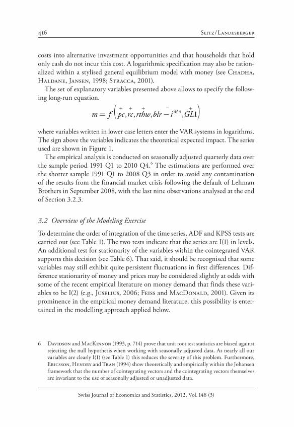
costs into alternative investment opportunities and that households that hold only cash do not incur this cost. A logarithmic specification may also be ration-alized within a stylised general equilibrium model with money (see Chadha, Haldane, Jansen, 1998; Stracca, 2001).

The set of explanatory variables presented above allows to specify the follow-ing long-run equation.

3, , , , 1Mm f pc rc rthw blr i GL

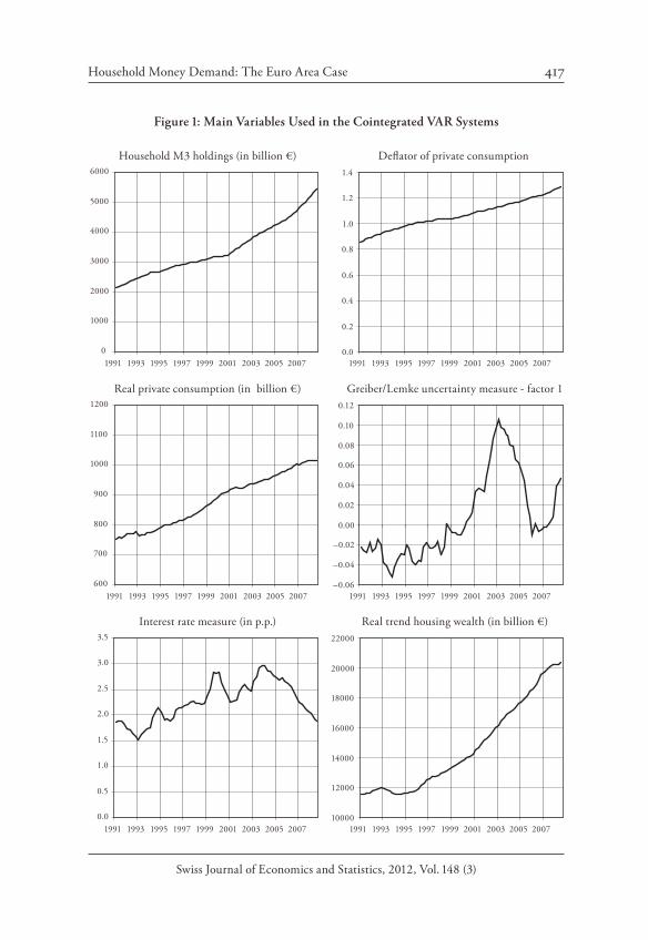
where variables written in lower case letters enter the VAR systems in logarithms. The sign above the variables indicates the theoretical expected impact. The series used are shown in Figure 1.

The empirical analysis is conducted on seasonally adjusted quarterly data over the sample period 1991 Q1 to 2010 Q4.6 The estimations are performed over the shorter sample 1991 Q1 to 2008 Q3 in order to avoid any contamination of the results from the financial market crisis following the default of Lehman Brothers in September 2008, with the last nine observations analysed at the end of Section 3.2.3.

3.2 Overview of the Modeling Exercise

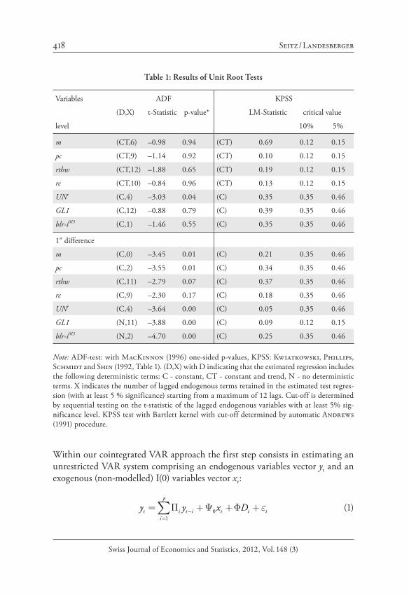
To determine the order of integration of the time series, ADF and KPSS tests are carried out (see Table 1). The two tests indicate that the series are I(1) in levels. An additional test for stationarity of the variables within the cointegrated VAR supports this decision (see Table 6). That said, it should be recognised that some variables may still exhibit quite persistent fluctuations in first differences. Dif-ference stationarity of money and prices may be considered slightly at odds with some of the recent empirical literature on money demand that finds these vari-ables to be I(2) (e.g., Juselius, 2006; Feiss and MacDonald, 2001). Given its prominence in the empirical money demand literature, this possibility is enter-tained in the modelling approach applied below.



0

1000

2000

3000

4000

5000

6000

1991 1993 1995 1997 1999 2001 2003 2005 2007

Household M3 holdings (in billion €) Deflator of private consumption

0.0

0.2

0.4

0.6

0.8

1.0

1.2

1.4

1991 1993 1995 1997 1999 2001 2003 2005 2007

Real private consumption (in billion €)

600

700

800

900

1000

1100

1200

1991 1993 1995 1997 1999 2001 2003 2005 2007

Greiber/Lemke uncertainty measure - factor 1

–0.06

–0.04

–0.02

0.00

0.02

0.04

0.06

0.08

0.10

0.12

1991 1993 1995 1997 1999 2001 2003 2005 2007

Interest rate measure (in p.p.)

0.0

0.5

1.0

1.5

2.0

2.5

3.0

3.5

1991 1993 1995 1997 1999 2001 2003 2005 2007

Real trend housing wealth (in billion €)

10000

12000

14000

16000

18000

20000

22000

1991 1993 1995 1997 1999 2001 2003 2005 2007

Figure : Main Variables Used in the Cointegrated VAR Systems



Within our cointegrated VAR approach the first step consists in estimating an unrestricted VAR system comprising an endogenous variables vector yt and an exogenous (non-modelled) I(0) variables vector xt :

01

p

t i t i t t ti

y y x D (1)

Table 1: Results of Unit Root Tests

Variables ADF KPSS

(D,X) t-Statistic p-value* LM-Statistic critical value

level 10% 5%

m (CT,6) –0.98 0.94 (CT) 0.69 0.12 0.15

pc (CT,9) –1.14 0.92 (CT) 0.10 0.12 0.15

rthw (CT,12) –1.88 0.65 (CT) 0.19 0.12 0.15

rc (CT,10) –0.84 0.96 (CT) 0.13 0.12 0.15

UNe (C,4) –3.03 0.04 (C) 0.35 0.35 0.46

GL1 (C,12) –0.88 0.79 (C) 0.39 0.35 0.46

blr-iM3 (C,1) –1.46 0.55 (C) 0.35 0.35 0.46

1st difference

m (C,0) –3.45 0.01 (C) 0.21 0.35 0.46

pc (C,2) –3.55 0.01 (C) 0.34 0.35 0.46

rthw (C,11) –2.79 0.07 (C) 0.37 0.35 0.46

rc (C,9) –2.30 0.17 (C) 0.18 0.35 0.46

UNe (C,4) –3.64 0.00 (C) 0.05 0.35 0.46

GL1 (N,11) –3.88 0.00 (C) 0.09 0.12 0.15

blr-iM3 (N,2) –4.70 0.00 (C) 0.25 0.35 0.46

Note: ADF-test: with MacKinnon (1996) one-sided p-values, KPSS: Kwiatkowski, Phillips, Schmidt and Shin (1992, Table 1). (D,X) with D indicating that the estimated regression includes the following deterministic terms: C - constant, CT - constant and trend, N - no deterministic terms. X indicates the number of lagged endogenous terms retained in the estimated test regres-sion (with at least 5 % significance) starting from a maximum of 12 lags. Cut-off is determined by sequential testing on the t-statistic of the lagged endogenous variables with at least 5% sig-nificance level. KPSS test with Bartlett kernel with cut-off determined by automatic Andrews (1991) procedure.



7 Lütkepohl and Saikonnen (1997, p. 16) find that “in most cases AIC and HQ have a slight advantage over the very parsimonious SC criterion”.

8 While normality of residuals is part of the theoretical assumptions of the distribution of resid-uals, the violation of normality may not be a severe deficiency as the evaluation of the trace test will be supported by bootstrapping results.

9 The cointegration analysis and the results presented in the remainder of this note are com-puted with the Structural VAR software which was kindly provided by Anders Warne. See http://www.texlips.net/svar/source.html. A cross-check of the VECM with single equation error correction models (even against the background that this is not justified according to our results) may be found in Seitz and von Landesberger (2010), Section 5.

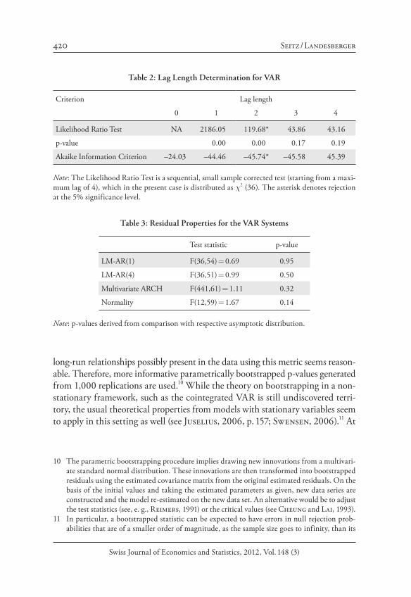
The errors t are assumed to be NI (0,Ω). i and are matrices containing the parameters of the model. Dt is a vector of deterministic variables, potentially comprising constant terms 0 or deterministic trends. Given the quarterly data used, the maximum lag length p is set equal to four in order to determine the appropriate number of lags for each model. The Akaike information criterion (AIC) is used to select the lag length for conducting the remainder of the analy-sis and the outcome is cross-checked with Likelihood Ratio tests (see Table 2). The AIC tends to favour the inclusion of more lagged terms than for example the Schwartz information criterion.7 Overestimation of the order of the VAR is much less serious than underestimating it, as shown for example by Kilian (2001). In our case, the two tests yield an unambiguous result of a lag length of 2 in levels. Table 3 presents the outcome of standard specification tests of the respective VAR system. The null of no autocorrelation in the residuals cannot be rejected at conventional significance levels. In a similar vein, tests for ARCH effects in the residuals and on the non-normality of the residuals are also not significant.8

In a second step, we reformulate the VAR system into a VECM and test for the rank of the matrix 1 using the trace test (see Johansen, 1996):

1

1 1 0 1 01

l

t t i t t ti

y y y x (2)

where l indicates the lag length determined in the previous step. The trace tests were conducted assuming the presence of a linear deterministic trend in the time series and a non-zero intercept 0 in the cointegration relationship.9

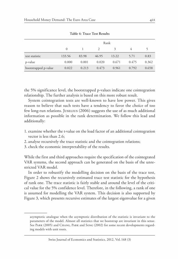
Table 4 reports the trace test statistics for different rank assumptions as well as the p-values obtained from comparing this test statistic with the critical values derived by MacKinnon, Haug and Michelis (1999). The model rejects the rank 0, 1 and 2 at the 5% significance level. However, given the presence of an exog-enous I(0) regressor and the small sample size, caution in assessing the number of



Table 2: Lag Length Determination for VAR

Criterion Lag length

0 1 2 3 4

Likelihood Ratio Test NA 2186.05 119.68* 43.86 43.16

p-value 0.00 0.00 0.17 0.19

Akaike Information Criterion –24.03 –44.46 –45.74* –45.58 45.39

Note: The Likelihood Ratio Test is a sequential, small sample corrected test (starting from a maxi-mum lag of 4), which in the present case is distributed as 2 (36). The asterisk denotes rejection at the 5% significance level.

Table 3: Residual Properties for the VAR Systems

Test statistic p-value

LM-AR(1) F(36,54) 0.69 0.95

LM-AR(4) F(36,51) 0.99 0.50

Multivariate ARCH F(441,61) 1.11 0.32

Normality F(12,59) 1.67 0.14

Note: p-values derived from comparison with respective asymptotic distribution.

10 The parametric bootstrapping procedure implies drawing new innovations from a multivari-ate standard normal distribution. These innovations are then transformed into bootstrapped residuals using the estimated covariance matrix from the original estimated residuals. On the basis of the initial values and taking the estimated parameters as given, new data series are constructed and the model re-estimated on the new data set. An alternative would be to adjust the test statistics (see, e. g., Reimers, 1991) or the critical values (see Cheung and Lai, 1993).

11 In particular, a bootstrapped statistic can be expected to have errors in null rejection prob-abilities that are of a smaller order of magnitude, as the sample size goes to infinity, than its

long-run relationships possibly present in the data using this metric seems reason-able. Therefore, more informative parametrically bootstrapped p-values generated from 1,000 replications are used.10 While the theory on bootstrapping in a non-stationary framework, such as the cointegrated VAR is still undiscovered terri-tory, the usual theoretical properties from models with stationary variables seem to apply in this setting as well (see Juselius, 2006, p. 157; Swensen, 2006).11 At



the 5% significance level, the bootstrapped p-values indicate one cointegration relationship. The further analysis is based on this more robust result.

System cointegration tests are well-known to have low power. This gives reason to believe that such tests have a tendency to favor the choice of too few long-run relations. Juselius (2006) suggests the use of as much additional information as possible in the rank determination. We follow this lead and additionally:

1. examine whether the t-value on the load factor of an additional cointegration vector is less than 2.6;

2. analyse recursively the trace statistic and the cointegration relations;3. check the economic interpretability of the results.

While the first and third approaches require the specification of the cointegrated VAR systems, the second approach can be generated on the basis of the unre-stricted VAR model.

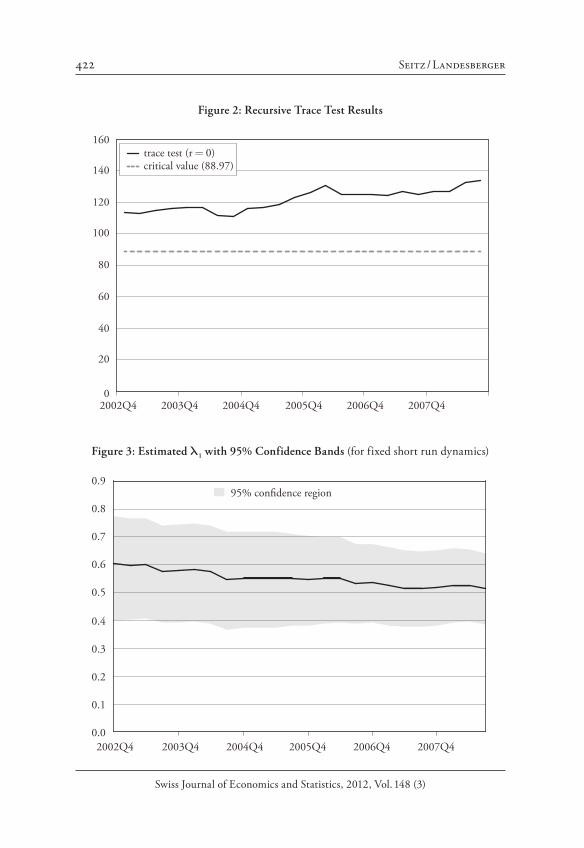
In order to robustify the modelling decision on the basis of the trace test, Figure 2 shows the recursively estimated trace test statistic for the hypothesis of rank one. The trace statistic is fairly stable and around the level of the criti-cal value for the 5% confidence level. Therefore, in the following, a rank of one is assumed for modelling the VAR system. This decision is also supported by Figure 3, which presents recursive estimates of the largest eigenvalue for a given

asymptotic analogue when the asymptotic distribution of the statistic is invariant to the parameters of the model. Almost all statistics that we bootstrap are invariant in this sense. See Park (2005) and Chang, Park and Song (2002) for some recent developments regard-ing models with unit roots.

Table 4: Trace Test Results

Rank

0 1 2 3 4 5

test statistic 133.56 83.98 46.95 13.22 5.71 0.83

p-value 0.000 0.001 0.020 0.671 0.475 0.362

bootstrapped p-value 0.022 0.213 0.473 0.961 0.792 0.658



Figure 2: Recursive Trace Test Results

0

20

40

60

80

100

120

140

160

2002Q4 2003Q4 2004Q4 2005Q4 2006Q4 2007Q4

trace test (r 0)critical value (88.97)

Figure 3: Estimated 1 with 95% Confidence Bands (for fixed short run dynamics)

2002Q4 2003Q4 2004Q4 2005Q4 2006Q4 2007Q40.0

0.1

0.2

0.3

0.4

0.5

0.6

0.7

0.8

0.995% confidence region



set of parameters of the short-run and deterministic variables. The depicted eigen-value band does not cross the zero line.

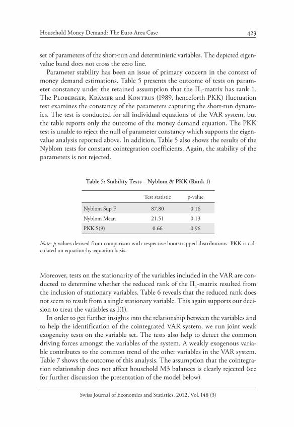
Parameter stability has been an issue of primary concern in the context of money demand estimations. Table 5 presents the outcome of tests on param-eter constancy under the retained assumption that the -matrix has rank 1. The Ploberger, Krämer and Kontrus (1989, henceforth PKK) fluctuation test examines the constancy of the parameters capturing the short-run dynam-ics. The test is conducted for all individual equations of the VAR system, but the table reports only the outcome of the money demand equation. The PKK test is unable to reject the null of parameter constancy which supports the eigen-value analysis reported above. In addition, Table 5 also shows the results of the Nyblom tests for constant cointegration coefficients. Again, the stability of the parameters is not rejected.

Table 5: Stability Tests – Nyblom & PKK (Rank 1)

Test statistic p-value

Nyblom Sup F 87.80 0.16

Nyblom Mean 21.51 0.13

PKK S(9) 0.66 0.96

Note: p-values derived from comparison with respective bootstrapped distributions. PKK is cal-culated on equation-by-equation basis.

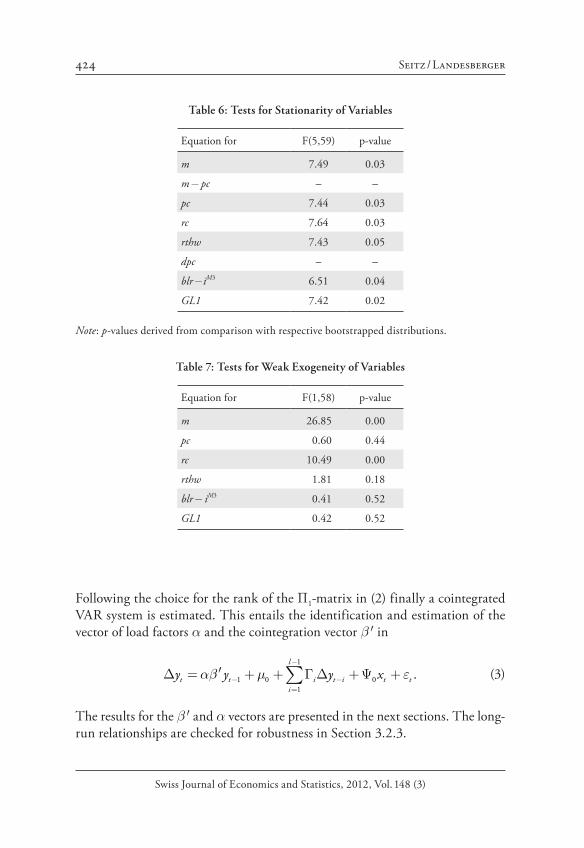
Moreover, tests on the stationarity of the variables included in the VAR are con-ducted to determine whether the reduced rank of the -matrix resulted from the inclusion of stationary variables. Table 6 reveals that the reduced rank does not seem to result from a single stationary variable. This again supports our deci-sion to treat the variables as I(1).

In order to get further insights into the relationship between the variables and to help the identification of the cointegrated VAR system, we run joint weak exogeneity tests on the variable set. The tests also help to detect the common driving forces amongst the variables of the system. A weakly exogenous varia-ble contributes to the common trend of the other variables in the VAR system. Table 7 shows the outcome of this analysis. The assumption that the cointegra-tion relationship does not affect household M3 balances is clearly rejected (see for further discussion the presentation of the model below).



Following the choice for the rank of the 1-matrix in (2) finally a cointegrated VAR system is estimated. This entails the identification and estimation of the vector of load factors and the cointegration vector in

1

1 0 01

.l

t t i t i t ti

y y y x (3)

The results for the and vectors are presented in the next sections. The long-run relationships are checked for robustness in Section 3.2.3.

Table 6: Tests for Stationarity of Variables

Equation for F(5,59) p-value

m 7.49 0.03

m pc – –

pc 7.44 0.03

rc 7.64 0.03

rthw 7.43 0.05

dpc – –

blr iM3 6.51 0.04

GL1 7.42 0.02

Note: p-values derived from comparison with respective bootstrapped distributions.

Table 7: Tests for Weak Exogeneity of Variables

Equation for F(1,58) p-value

m 26.85 0.00

pc 0.60 0.44

rc 10.49 0.00

rthw 1.81 0.18

blr iM3 0.41 0.52

GL1 0.42 0.52



12 The test statistic is distributed as F(1,59) 0.31 (p-value 0.58).

3.2.1 The Long-Run Relationships – the s

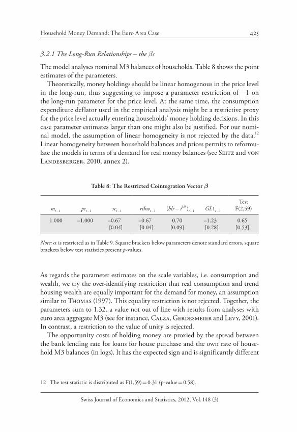
The model analyses nominal M3 balances of households. Table 8 shows the point estimates of the parameters.

Theoretically, money holdings should be linear homogenous in the price level in the long-run, thus suggesting to impose a parameter restriction of 1 on the long-run parameter for the price level. At the same time, the consumption expenditure deflator used in the empirical analysis might be a restrictive proxy for the price level actually entering households’ money holding decisions. In this case parameter estimates larger than one might also be justified. For our nomi-nal model, the assumption of linear homogeneity is not rejected by the data.12 Linear homogeneity between household balances and prices permits to reformu-late the models in terms of a demand for real money balances (see Seitz and von Landesberger, 2010, annex 2).

Table 8: The Restricted Cointegration Vector

mt 1 pct 1 rct 1 rthwt 1 (blr iM3 )t 1 GL1t 1

TestF(2,59)

1.000 –1.000 –0.67[0.04]

–0.67[0.04]

0.70[0.09]

–1.23[0.28]

0.65[0.53]

Note: is restricted as in Table 9. Square brackets below parameters denote standard errors, square brackets below test statistics present p-values.

As regards the parameter estimates on the scale variables, i.e. consumption and wealth, we try the over-identifying restriction that real consumption and trend housing wealth are equally important for the demand for money, an assumption similar to Thomas (1997). This equality restriction is not rejected. Together, the parameters sum to 1.32, a value not out of line with results from analyses with euro area aggregate M3 (see for instance, Calza, Gerdesmeier and Levy, 2001). In contrast, a restriction to the value of unity is rejected.

The opportunity costs of holding money are proxied by the spread between the bank lending rate for loans for house purchase and the own rate of house-hold M3 balances (in logs). It has the expected sign and is significantly different



from zero (at the 5% percent level). However, with 0.7 the parameter estimate is relatively large. The sign on the financial market uncertainty measure in the long-run relationship has the expected positive sign and is significantly differ-ent from zero, implying that higher financial market uncertainty leads to higher money holdings.

The long-run determinants discussed above are augmented by expectations with regard to unemployment over the coming twelve months UN e from the survey of the EU Commission. It only enters the short-run dynamics of the system. A deteriorating employment situation may, on the one hand, induce households to hold more money balances to meet unforeseen expenditures. On the other hand, the expected deteriorating economic environment and increasing uncertainty may reduce the attractiveness of nominal assets and induce the pur-chase of more real assets. Therefore, the overall impact on the demand for money is ambiguous (see Atta-Mensah, 2004). The point estimate is negative which is in line with Atta-Mensah (2004) for Canada. Obviously, this reflects the fact that over the sample the effect via precautionary money holdings dominates.

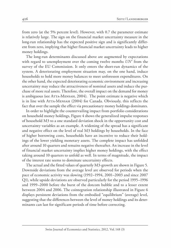
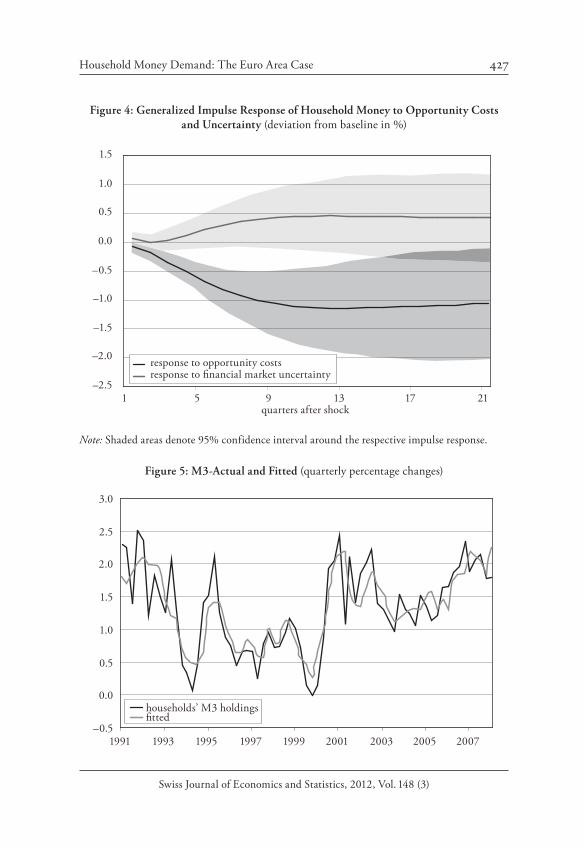
In order to highlight the countervailing impact from portfolio considerations on household money holdings, Figure 4 shows the generalized impulse responses of household M3 to a one standard deviation shock in the opportunity cost and uncertainty variables as an example. A widening of the spread has a significant and negative effect on the level of real M3 holdings by households. In the face of higher borrowing costs, households have an incentive to reduce their hold-ings of the lower yielding monetary assets. The complete impact has unfolded after around 10 quarters and remains negative thereafter. An increase in the level of financial market uncertainty implies higher money holdings, with the effect taking around 10 quarters to unfold as well. In terms of magnitude, the impact of the interest rate seems to dominate uncertainty effects.

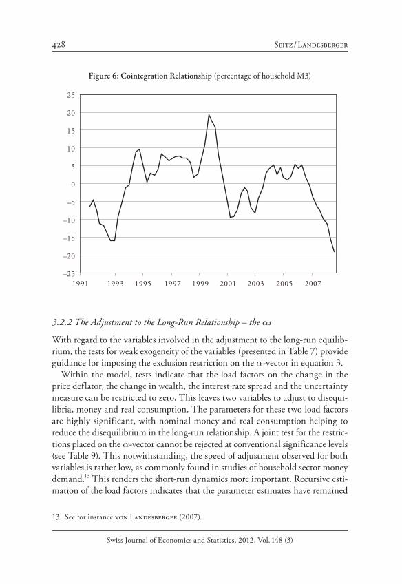
The actual and the fitted values of quarterly M3-growth are shown in Figure 5. Downside deviations from the average level are observed for periods when the pace of economic activity was slowing (1992–1994, 2001–2003 and since 2007 Q1), while upside deviations are observed particularly for the period 1995–1996 and 1999–2000 before the burst of the dotcom bubble and to a lesser extent between 2004 and 2006. The cointegration relationship illustrated in Figure 6 displays persistent deviations from the embodied “equilibrium” (average) level, suggesting that the differences between the level of money holdings and its deter-minants can last for significant periods of time before correcting.



Figure 4: Generalized Impulse Response of Household Money to Opportunity Costs and Uncertainty (deviation from baseline in %)

–2.5

–2.0

–1.5

–1.0

–0.5

0.0

0.5

1.0

1.5

1 5 9 13 17 21quarters after shock

response to opportunity costsresponse to financial market uncertainty

Note: Shaded areas denote 95% confidence interval around the respective impulse response.

Figure 5: M3-Actual and Fitted (quarterly percentage changes)

–0.5

0.0

0.5

1.0

1.5

2.0

2.5

3.0

1991 1993 1995 1997 1999 2001 2003 2005 2007

fittedhouseholds’ M3 holdings



Figure 6: Cointegration Relationship (percentage of household M3)

–25

–20

–15

–10

–5

0

5

10

15

20

25

1991 1993 1995 1997 1999 2001 2003 2005 2007

3.2.2 The Adjustment to the Long-Run Relationship – the s

With regard to the variables involved in the adjustment to the long-run equilib-rium, the tests for weak exogeneity of the variables (presented in Table 7) provide guidance for imposing the exclusion restriction on the -vector in equation 3.

Within the model, tests indicate that the load factors on the change in the price deflator, the change in wealth, the interest rate spread and the uncertainty measure can be restricted to zero. This leaves two variables to adjust to disequi-libria, money and real consumption. The parameters for these two load factors are highly significant, with nominal money and real consumption helping to reduce the disequilibrium in the long-run relationship. A joint test for the restric-tions placed on the -vector cannot be rejected at conventional significance levels (see Table 9). This notwithstanding, the speed of adjustment observed for both variables is rather low, as commonly found in studies of household sector money demand.13 This renders the short-run dynamics more important. Recursive esti-mation of the load factors indicates that the parameter estimates have remained

13 See for instance von Landesberger (2007).



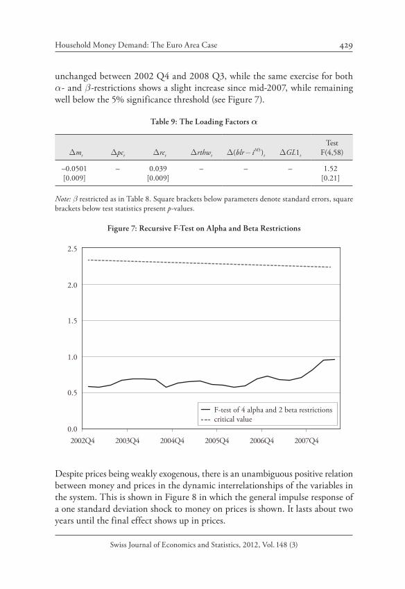
unchanged between 2002 Q4 and 2008 Q3, while the same exercise for both - and -restrictions shows a slight increase since mid-2007, while remaining

well below the 5% significance threshold (see Figure 7).

Table 9: The Loading Factors

mt

pct

rct

rthwt

(blr iM3 )t

GL1t

Test F(4,58)

–0.0501[0.009]

– 0.039[0.009]

– – – 1.52[0.21]

Note: restricted as in Table 8. Square brackets below parameters denote standard errors, square brackets below test statistics present p-values.

Figure 7: Recursive F-Test on Alpha and Beta Restrictions

0.0

0.5

1.0

1.5

2.0

2.5

2002Q4 2003Q4 2004Q4 2005Q4 2006Q4 2007Q4

critical valueF-test of 4 alpha and 2 beta restrictions

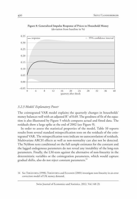
Despite prices being weakly exogenous, there is an unambiguous positive relation between money and prices in the dynamic interrelationships of the variables in the system. This is shown in Figure 8 in which the general impulse response of a one standard deviation shock to money on prices is shown. It lasts about two years until the final effect shows up in prices.



14 See Teräsvirta (1998); Teräsvirta and Eliasson (2001) investigate non-linearity in an error correction model of UK money demand.

Figure 8: Generalized Impulse Response of Prices to Household Money (deviation from baseline in %)

0.35

0.30

0.25

0.20

0.15

0.10

0.05

0.00

–0.050 4 8 12 16 20 24 28 32 36 40

quarters after shock

response 95% confidence interval

3.2.3 Models’ Explanatory Power

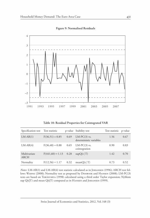
The cointegrated VAR model explains the quarterly changes in households’ money balances well with an adjusted R2 of 0.69. The goodness of fit of the equa-tion is also illustrated by Figure 5 which compares actual and fitted data. The residuals show a large spike at the end of 2002 (see Figure 9).

In order to assess the statistical properties of the model, Table 10 reports results from several standard misspecification tests on the residuals of the coin-tegrated VAR. The misspecification tests indicate no autocorrelation of residuals. Multivariate ARCH effects as well as non-normality can also not be detected. The Nyblom tests conditional on the full sample estimates for the constant and the lagged endogenous parameters do not reveal any instability of the long-run parameters. Finally, the LM-tests against the alternative of non-linearity in the deterministic variables or the cointegration parameters, which would capture gradual shifts, also do not reject constant parameters.14



Figure 9: Normalised Residuals

–3

–2

–1

0

1

2

3

4

1991 1993 1995 1997 1999 2001 2003 2005 2007

Table 10: Residual Properties for Cointegrated VAR

Specification test Test statistic p-value Stability test Test statistic p-value

LM-AR(1) F(36,51) 0.85 0.69 LM-PC(3) vs. deterministic variables

1.56 0.67

LM-AR(4) F(36,48) 0.88 0.65 LM-PC(3) vs. cointegration

0.90 0.83

Multivariate ARCH

F(441,60) 1.13 0.28 supQ(t T) 1.42 0.70

Normality F(12,56) 1.17 0.32 meanQ(t T) 0.73 0.52

Notes: LM-AR(1) and LM-AR(4) test statistic calculated as in Johansen (1996); ARCH test fol-lows Warne (2008); Normality test as proposed by Doornik and Hansen (2008); LM-PC(3) tests are based on Teräsvirta (1998) calculated using a third order Taylor expansion; Nyblom sup Q(t|T) and mean Q(t|T) computed as in Hansen and Johansen (1999).



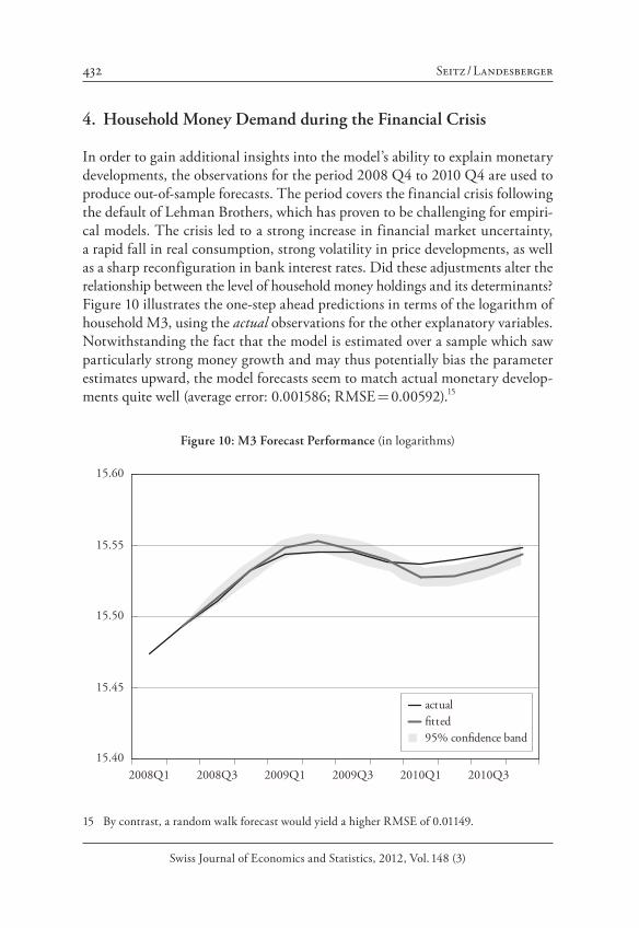
15 By contrast, a random walk forecast would yield a higher RMSE of 0.01149.

4. Household Money Demand during the Financial Crisis

In order to gain additional insights into the model’s ability to explain monetary developments, the observations for the period 2008 Q4 to 2010 Q4 are used to produce out-of-sample forecasts. The period covers the financial crisis following the default of Lehman Brothers, which has proven to be challenging for empiri-cal models. The crisis led to a strong increase in financial market uncertainty, a rapid fall in real consumption, strong volatility in price developments, as well as a sharp reconfiguration in bank interest rates. Did these adjustments alter the relationship between the level of household money holdings and its determinants? Figure 10 illustrates the one-step ahead predictions in terms of the logarithm of household M3, using the actual observations for the other explanatory variables. Notwithstanding the fact that the model is estimated over a sample which saw particularly strong money growth and may thus potentially bias the parameter estimates upward, the model forecasts seem to match actual monetary develop-ments quite well (average error: 0.001586; RMSE 0.00592).15

Figure 10: M3 Forecast Performance (in logarithms)

15.40

15.45

15.50

15.55

15.60

2008Q1 2008Q3 2009Q1 2009Q3 2010Q1 2010Q3

actualfitted95% confidence band



Additional evidence on the impact of the financial crisis on the relationship between household money holdings and macroeconomic developments can be obtained from re-estimating the model over the extended sample until the end of 2010. The outcome of the trace test still favours one cointegration relationship when using the bootstrapped distribution. The long-run parameter estimates over the extended sample are higher than those of the original sample, for instance, the consumption elasticity of money holdings increases from 0.67 to 0.82. However, the differences are not significant when compared with a bootstrapped F-test. In contrast, some of the misspecification tests deteriorate somewhat: Specifically, indication for non-normality of the residuals can be found. Closer inspection of the individual residuals indicates that this is due to the equations explaining real consumption. It seems that during the crisis period the dynamics of the variables, especially of housing wealth and, to a lesser extent, of the interest rate differen-tial change with regard to the pre-crisis sample. In contrast, the dynamic effect of these variables on money demand and real consumption have only marginally changed. Overall, given the magnitude of shocks implied by the financial crisis with regard to both the slowdown in consumption and housing wealth as well as the unprecedented change in the pass-trough of bank interest rates, the model over the extended sample still remains surprisingly similar to the original specification.

5. Summary and Conclusion

The results presented suggest that the model describes money demand by euro area households in a satisfactory manner, when judged, for instance, by the in-sample fit and standard misspecification tests. In addition, the estimates for the parameters allow for a theory-consistent interpretation and thereby support the view that money demand relationships have been identified.

In the euro area, household holdings of M3 are informative with regard to developments in inflation. An empirical framework permitting to analyse the driving factors for household money demand is therefore an important element for monetary analysis. The paper presented one approach at the household level to model the demand for nominal M3 balances in the euro area. It incorporates precautionary motives of holding money and the portfolio allocation process. In investigating the long-run relationship between money, two scale variables, opportunity costs and uncertainty, only a few combinations may satisfy formal cointegration tests, even if an underlying cointegration relationship is present for a broader set of similar variables (see Ericsson, 1998). Several important out-comes have been found:



16 At the same time, the inclusion of consumer expectations with regard to economic activity is able to offset this increase (see Seitz and von Landesberger, 2010). This may reflect the fact that, in theory, wealth captures expectations on the future income path.

17 The latter is not shown but available upon request.

1. The model does not reject linear homogeneity between money balances and the price level. It therefore supports the specification in real terms and sug-gests that in the long-run households are not subject to money illusion, in line with theoretical considerations.

2. Household money balances are never weakly exogenous with regard to the other variables of the cointegrated VAR and therefore always adjust to dise-quilibria between (real) money and its long-run determinants. That said, the model also provides evidence that the volume of transactions (proxied by real consumption) is affected by monetary disequilibria and also adjusts. By con-trast, the other variables are found to be the forces jointly determining the growth of money and real consumption in the long-run.

3. In explaining households’ broad money balances, it seems that housing wealth in conjunction with real consumption expenditures best capture households’ notional level of money holdings. Omitting wealth from the specification leads to a sizeable increase in the income elasticity of money demand.16

4. Interest rate developments seem to play a significant role for the development of household balances. The model specified with a double log formulation for opportunity costs exhibits a markedly stronger impact than is the case for the semi-log functional form.17 An increase in opportunity costs leads to a signifi-cant decline in money holdings with the effect fully materialising after about 10 quarters.

5. The model suggests that the impact of uncertainty on household balances is positive. Correctly incorporating the persistent behaviour of interest rates and uncertainty into the money demand function is essential to adequately cap-ture the driving forces impacting on money and expenditures as well as their mutual interaction.

While these results may not be seen as surprising as the estimates are consistent with results reported in the literature, the exercises presented help to better iden-tify the determinants of euro area money demand and to interpret current mon-etary developments. Extending the sample to include the crisis period, the new estimates indicate some minor changes, the key elements of the model described above, however, remain valid. As households’ money demand captures the bulk of aggregate euro area M3, it should also be helpful in understanding the long-run money-price-nexus.



More generally, the exercise also provides insights that go beyond the portfolio allocation decision of households. According to our analysis, it is quite apparent that in equilibrium, households jointly determine consumption and broad money holdings both influenced by wealth as well as interest rates. The importance of household money holdings for consumption expenditures may cast doubt on a purely passive role for money in this context. Moreover, as both bank lending rates and the own rate of households M3 are found significant, the determina-tion of money holdings seems to interact with wealth and indebtedness. In order to be able to more fully analyse the interaction between money holdings, con-sumption and wealth, the financing of households needs to be modelled as well, which goes beyond the scope of the present paper.

References

Adalid, Ramón, and Carsten Detken (2007), “Liquidity Shocks and Asset Price Boom/Bust Cycles”, ECB Working Paper No. 732.

Anderson, Richard, and Sean Collins (1997), “Modelling US Households’ Demand for Liquid Wealth in an Era of Financial Change”, Journal of Money, Credit and Banking 30(1),pp. 82–101.

Atta-Mensah, Joseph (2004), “Money Demand and Economic Uncertainty”, Bank of Canada Working Paper 2004-25.

Attanasio, Orazio, Guiso, Luigi, and Tullio Jappelli (1998), “The Demand for Money, Financial Innovation, and the Welfare cost of Inflation: An Anal-ysis with Household Data”, National Bureau of Economic Research Work-ing Paper 6593.

Beyer, Andreas (2009), “A Stable Model for Euro Area Money Demand: Revis-iting the Role of Wealth”, ECB Working Paper No. 1111.

Boone, Laurence, and Paul van den Noord (2008), “Wealth Effects on Money Demand in the Euro Area”, Empirical Economics 34(2),pp. 525–536.

Butkiewicz, James J. and Margaret M. McConnell (1995), “The Stability of the Demand for Money and M1 Velocity: Evidence from the Sectoral Data”, Quarterly Review of Economics and Finance 35(3), pp. 233–243.

Calza, Alessandro, Dieter Gerdesmeier, and Joaquim Levy (2001), “Euro Area Money Demand: Measuring the Opportunity Costs Appropriately”, IMF Working Paper 01/179.

Chadha, Jagijt, Haldane, Andrew and Norbert Janssen (1998), “Shoe Leather Costs Reconsidered”, Economic Journal 108(447), pp. 363–382.



Chang, Yoosoon, Joon Y. Park, and Kevin Song (2002), “Bootstrapping Cointegrating Regressions”, Department of Economics Working Paper 2002-04, Rice University.

Cheung, Yin-Wong, and Kon S. Lai (1993), “Finite-Sample Sizes of Johansen’s Likelihood Ratio Tests for Cointegration”, Oxford Bulletin of Economics and Statistics 55(3), pp. 313–328.

Chrystal, Alec, and Paul Mizen (2001), “Consumption, Money and Lend-ing: A Joint Model for the UK Household Sector”, Bank of England Work-ing Paper 134.

Davidson, Russell, and James G. MacKinnon (1993), Estimation and Infer-ence in Econometrics, New York, Oxford: Oxford University Press.

de Bondt, Gabe (2009), “Euro Area Money Demand: Empirical Evidence on the Role of Equity and Labour Markets”, ECB Working Paper No. 1068.

Detken, Carsten, and Frank Smets (2004), “Asset Price Booms and Mon-etary Policy”, ECB Working Paper 364, May.

Doornik, Jurgen A., and Henrik Hansen (2008), “An Omnibus Test for Univariate and Multivariate Normality”, Oxford Bulletin of Economics and Statistics, 70, pp. 927–939.

Ericsson, Neil R. (1998), “Empirical Modelling of Money Demand”, Empiri-cal Economics 23(3), pp. 295–315.

Ericsson, Neil R., David F. Hendry and Hong-Anh Tran (1994), “Coin-tegration, Seasonality, Encompassing, and the Demand for Money in the United Kingdom”, in: C. Hargreaves (ed.), Non-stationary Time-series Analysis and Cointegration, pp. 179–224, Oxford: Oxford University Press.

European Central Bank (2006), “Sectoral Money Holdings and the Infor-mation Content of Money with Respect to Inflation”, Box 1, Monthly Bul-letin, September, pp. 18–20.

Feiss, Norbert, and Ronald MacDonald (2001), “The Instability of the Money Demand Function, an I(2) Interpretation”, Oxford Bulletin of Eco-nomics and Statistics 63(4), pp. 475–495.

Friedman, Milton (1956), Studies in the Quantity Theory of Money, Chicago: University of Chicago Press.

Fujiki, Hiroshi, and Cheng Hsiao (2008), “Aggregate and Household Demand for Money, Evidence from Public Opinion Survey on Household Financial Assets and Liabilities”, Bank of Japan Institute of Monetary and Economic Studies Discussion Working Paper No. 2008-E-17.

Garver, Cecily, and Laurence Radecki (1987), “The Household Demand for Money, Estimates from Cross-Sectional Data”, Federal Reserve Bank of New York Quarterly Review, Spring, pp. 29–34.



Gerdesmeier, Dieter (1996), „Die Rolle des Vermögens in der Geldnach-frage“, Discussion paper 96/5, Volkswirtschaftliche Forschungsgruppe der Deutschen Bundesbank.

Goldfeld, Stephan (1973), “The Demand for Money Revisited”, Brookings Papers on Economic Activity 1973(3), pp. 577–646.

Greiber, Claus, and Wolfgang Lemke (2005), “Money Demand and Mac-roeconomic Uncertainty”, Deutsche Bundesbank Discussion Paper 26-2005.

Greiber, Claus, and Ralph Setzer (2007), “Money and Housing, Evidence for the Euro Area and the US”, Deutsche Bundesbank Discussion Paper 12-2007.

Hansen, Henrik, and Søren Johansen (1999), “Some Tests for Parameter Con-stancy in Cointegrated VAR-Models”, Econometrics Journal 2(2), pp. 306–333.

Jain, Parul, and Choon-Geol Moon (1994), “Sectoral Money Demand, a Coin-tegration Approach”, Review of Economics and Statistics 76(1), pp. 196–202.

Johansen, Søren (1996), Likelihood-Based Inference in Cointegrated Vector Autoregressive Models, 2nd ed., Oxford: Oxford University Press.

Juselius, Katerina (2006), The Cointegrated VAR Model, Methodology and Applications, Oxford: Oxford University Press.

Kilian, Lutz (2001), “Impulse Response Analysis in Vector Autoregressions with Unknown Lag Order”, Journal of Forecasting 20(3), pp. 161–179.

Kwiatkowski, Denis, Peter C. B. Phillips, Peter Schmidt, and Yongcheol Shin (1992), “Testing the Null Hypothesis of Stationarity against the Alter-native of a Unit Root”, Journal of Econometrics 54(1–3), pp. 159–178.

Laumas, Gurcharan S. (1979), “The Stability of the Demand for Money by the Household Sector, A Note”, Southern Economic Journal 46(2), pp. 603–608.

Lucas, Robert (2000), “Inflation and Welfare”, Econometrica 68(2), pp. 247–274.Lütkepohl, Helmut, and Pentti Saikkonen (1997), “Order Selection in

Testing for the Cointegrating Rank of a VAR Process”, Sonderforschungs-bereich 373, Quantification and Simulation of Economic Processes 93 (SFB 373 Papers).

MacKinnon, James G. (1996), “Numerical Distribution Functions for Unit Root and Cointegration Tests”, Journal of Applied Econometrics 11(6), pp. 601–618.

Martinez-Carrascal, Carmen, and Julian von Landesberger (2010), “Explaining the Money Demand of non-Financial Corporations in the Euro Area, A Macro and a Micro View”, ECB Working Paper No. 1257.

Park, Joon Y. (2003), “Bootstrap Unit Root Tests”, Econometrica 71(6), pp. 1845–1895.

Petursson, Thorarinn (2000), “The Representative Household’s Demand for Money in a Cointegrated VAR Model”, Econometrics Journal 3(2), pp. 162–176.



Read, Vicky (1996), “Sectoral Disaggregation of German M3”, Deutsche Bun-desbank Discussion Paper 1-1996.

Reimers, Hans-Eggert (1991), “Comparisons of Tests for Multivariate Coin-tegration”, Statistical Papers 33, pp. 335–359.

Seitz, Franz, and Julian von Landesberger (2010), “Household Money Holdings in the Euro Area, an Explorative Investigation”, ECB Working Paper No. 1238.

Stracca, Livio (2001), “The Functional Form of the Demand for Euro Area M1”, The Manchester School 71(2), pp. 172–204.

Swensen, Anders R. (2006), “Bootstrap Algorithms for Testing and Determining the Cointegration Rank in VAR Models”, Econometrica 74(6), pp. 1699–1714.

Teräsvirta, Timo (1998), “Modelling Economic Relationships with Smooth Transition Regressions”, in Handbook of Applied Economic Statistics, Aman Ullah and David E.A. Giles (eds), pp. 507–552, New York et al.: Dekker.

Teräsvirta, Timo, and Ann Charlotte Eliasson (2001), “Non-Linear Error Correction and the UK Demand for Broad Money”, 1878–1993, Journal of Applied Econometrics 16(3), pp. 277–288.

Thomas, Ryland (1997), “The Demand for M4, A Sectoral Analysis Part 1 – The Personal Sector”, Bank of England Working Paper 61.

Tobin, James (1969), “A General Equilibrium Approach to Monetary Theory”, Journal of Money, Credit and Banking, 1(1), pp. 15–29.

von Landesberger, Julian (2007), “Sectoral Money Demand Models for the Euro Area Based on a Common Set of Determinants”, ECB Working Paper No. 741.

Warne, Anders (2008), Structural VAR, version 0.50, release 1.

SUMMARY

In this paper we analyse household holdings of the broad monetary aggregate M3 in the euro area from 1991 until 2010. We develop a nominal model with satisfactory economic and statistical properties. The main determinants are a transactions variable, wealth considerations, opportunity costs and uncertainty. The model is robust to different samples considered and a multitude of mis-spec-ification tests. The exercise also provides insights that go beyond the portfolio allocation decision of households. According to our analysis, it is quite apparent that in equilibrium, households jointly determine consumption and broad money holdings both influenced by wealth as well as interest rates.

Date post:	01-Jan-2017
Category:	Documents
Upload:	nguyentuyen
View:	217 times
Download:	0 times

3 Schweizerische Zeitschrift für Volkswirtschaft und Statistik Revue ...

Documents